arX

iv:0

903.

3222

v2 [

hep-

th]

19

Mar

200

9

Preprint typeset in JHEP style - HYPER VERSION LPTENS-09/07

3D Seiberg-like Dualities and M2 Branes

Antonio Amariti1,a, Davide Forcella2,b, Luciano Girardello1,c and Alberto Mariotti3,d

1Dipartimento di Fisica, Universita di Milano Bicocca

and

INFN, Sezione di Milano-Bicocca,

piazza della Scienza 3, I-20126 Milano, Italy

2 Laboratoire de Physique Theorique de l’Ecole Normale Superieure

and

CNRS UMR 8549

24 Rue Lhomond Paris 75005, France

3 Theoretische Natuurkunde, Vrije Universiteit Brussel

and

The International Solvay Institutes

Pleinlaan 2, B-1050 Brussels, Belgium

aantonio.amariti@mib.infn.it bforcella@lpt.ens.frcluciano.girardello@mib.infn.it dalberto.mariotti@vub.ac.be

Abstract: We investigate features of duality in three dimensional N = 2 Chern-Simons

matter theories conjectured to describe M2 branes at toric Calabi Yau four-fold singulari-

ties. For 3D theories with non-chiral 4D parents we propone a Seiberg-like duality which

turns out to be a toric duality. For theories with chiral 4D parents we discuss the conditions

under which that Seiberg-like duality leads to toric duality. We comment on such duality

in 3D theories without 4D parents.

Contents

1. Introduction 1

2. M2 branes and N = 2 Chern Simons theories 3

2.1 An Algorithm to compute M4 5

3. Non-Chiral Theories 6

3.1 Seiberg-like duality 7

3.2 L121{k1,k2,k3} 9

3.3 L222{ki} 11

3.4 The general Laba{ki} 12

4. Chiral theories 16

4.1 F0{ki} 17

4.2 dP1{ki} 19

4.3 dP2{ki} 20

4.4 dP3{ki} 21

4.5 Y 32{ki} 23

5. Dualities for CS theories without 4d parents 23

5.1 Example 24

6. Conclusion 25

A. Parity anomaly 26

1. Introduction

Different descriptions of the same physical phenomenon usually provide a better under-

standing of the phenomenon itself. AdS/CFT correspondence and Seiberg duality are two

famous examples. In the AdS5/CFT4 case it happens that to a single geometry correspond

different UV field theory descriptions. This phenomenon was called Toric Duality in [1],

analyzed in [2, 3] and identified as a Seiberg duality in [4, 5]. Due to the difficulties to

understand the field theory living on M2 branes the AdS4/CFT3 correspondence was less

mastered. An important step in this direction has been the realization of the importance

of Chern-Simons interactions [6] and the subsequent construction of N = 8 Chern-Simons

matter field theories in [7, 10, 8, 9, 10, 11, 12, 13]. A breakthrough toward the explicit

realization of the AdS4/CFT3 correspondence was done in [14] where the authors propose

– 1 –

U(N)k × U(N)−k CS matter theories, with N = 6 supersymmetry, to be the low energy

theories of N M2-branes at the C4/Zk singularities. Afterwards, this construction has

been extended to many others CS matter theories with a lower amount of supersymmetries

[15, 16, 17, 18, 19, 20, 21, 22, 23, 24, 25, 26, 27].

A large and interesting, but still very peculiar, class of AdS4/CFT3 pairs is realized

by M2 branes at Calabi Yau four-fold toric singularities [19, 20, 21, 26, 27, 28, 29]. The

low energy theories are proposed to be a special kind of N = 2 Chern-Simons matter

theories. It was soon realized [21] that, as in the AdS5/CFT4 case, different N = 2 Chern-

Simons matter theories can be associated with the same Calabi Yau fourfold geometry. The

phenomenon of toric duality reappears in the AdS4/CFT3 correspondence, but in a much

general context. Indeed, contrary to the four dimensional case, in three dimensions one

find models with different numbers of gauge group factors to describe the same IR physics

(for example mirror symmetry pairs [30]). In the literature some very specific pairs of dual

field theories were constructed. A step was done in [31, 32] where a sort of Seiberg like

duality for three dimensional Chern-Simons matter theory was proposed1. In the context

of M2 branes at singularities, we can divide the set of dualities in the ones that change and

in the ones that do not change the number of gauge group factors. In this paper we will

call the second type of duality Seiberg-like toric duality.

N = 2 Chern-Simons matter theories for M2 branes at singularities are typically

described by a quiver with an assignment of Chern-Simons levels ki and a superpotential

in a way similar to the gauge theories for D3 branes at Calabi Yau three-fold singularities.

Indeed a class of N = 2 three dimensional theories can be simply obtained from four

dimensional N = 1 quivers with superpotential in the following way: rewrite the theory in

three dimensions, change the SU(N) gauge factors to U(N) factors, disregard the super

Yang-Mills actions and add a super Chern-Simons term for every factors. We will say that

these three dimensional theories have a four dimensional parent. Viceversa we will call

theories without four dimensional parents the three dimensional theories that cannot be

obtained in the way just explained [27].

In this paper we investigate Seiberg-like toric dualities for (2+1) dimensional N = 2

Chern-Simons matter theories associated with M2 branes at Calabi Yau four-fold toric

singularities. Using a generalization of the forward algorithm for D3 branes [26] we analyze

a particular branch of the moduli space that is supposed to reproduce the transverse four-

fold Calabi Yau singularity. We identify a set of Seiberg-like toric dualities for three

dimensional Chern-Simons quiver theories.

For theories with four dimensional parents one could try to simply extend the four

dimensional Seiberg duality to the three dimensional case. In fact, three dimensional the-

ories share the same Master Spaces [35, 36] of their four dimensional parents. In the map

between four and three dimensions a direction of the Master Space become a direction

of the physical Calabi Yau four-fold. Unfortunately, it turns out that an arbitrary as-

signment of 2+1 dimensional Chern-Simons levels does not in general commute with 3+1

dimensional Seiberg duality [21]. In fact it was shown in [37] that the Master Space for

1Seiberg duality for 3D gauge theories were previously studied in [33, 34].

– 2 –

four dimensional Seiberg dual theories are not in general isomorphic. Actually it seems

that three dimensional CS theories with chiral four dimensional parents do not admit a

simple generalization of the three dimensional SQCD Seiberg duality as it happens in the

four dimensional case.

Here, we first analyze non chiral three dimensional CS theories with (3+1)d parents.

Using a type IIB brane realization, we propose a Seiberg like duality, with a precise

prescription for the transformation of the CS levels and the gauge groups factors. We then

check that this proposed Seiberg like duality is indeed a toric duality, namely that the

two dual theories are associated with M2 branes probing the same Calabi Yau four-fold

singularity.

We try to simply extend to chiral CS theories with (3+1)d parents the rules that we

have found for the non chiral theories. For chiral four dimensional theories the Master Space

is not isomorphic among Seiberg dual phases [37]. This fact presumably puts constraints on

the duality transformations for the three dimensional case. We find indeed difficulties for a

straightforward realization of Seiberg like toric dualities for 2+1 dimensional Chern-Simons

matter theories with four dimensional chiral parents.

However, by analyzing several examples, we find a rule for the assignments of the CS

levels such that toric duality still holds among Seiberg like dual phases.

We finally give some examples of Chern-Simons theories without four dimensional

parents. In this case there is no immediate insight from the four dimensions, but we show

that the duality proposed for the chiral theories works also for theories without a 3+1

parents.

Our analysis is a first step to the study of Seiberg-like toric dualities in the context

of M2 branes. We tried to use the intuition from the non-chiral case and to leave as

arbitrary as possible the values of the Chern-Simons levels. It is reasonable that more

general transformation rules exist. Moreover it would be nice to investigate more general

families of toric dualities, like the ones changing the number of gauge group factors and

the large limit for Chern-Simons levels. We leave these topics for future investigations.

As we were finishing this paper, we were informed of [54, 55] which discuss related

topics.

2. M2 branes and N = 2 Chern Simons theories

As discussed in the introduction, supersymmetric Chern Simons theories coupled to matter

fields are good candidates to describe the low energy dynamics of M2 branes [6, 14]. In this

paper we are interested in M2 branes at Calabi Yau four fold toric conical singularities.

The authors of [20] proposed that the field theories living on these M2 branes are (2+1) di-

mensional N = 2 Chern Simons theories with gauge group∏G

i=1 Ui(N) with bifundamental

and adjoint matter fields. The Lagrangian in N = 2 superspace notation is:

Tr

−i

∑

a

ka

∫ 1

0dtVaD

α(etVaDαe−tVa) −

∫d4θ

∑

Xab

X†abe

−VaXabeVb +

∫d2θW (Xab) + c.c.

(2.1)

– 3 –

where Va are the vector superfields and Xab are bifundamental chiral superfields. The

superpotential W (Xab) satisfies the toricity conditions: every field appears just two times:

one time with plus sign and the other time with minus sign. Since these theories are

conjectured to be dual to M theory on AdS4×SE7, where SE7 is a seven dimensional Sasaki

Einstein manifold, the moduli space of these theories must contain a branch isomorphic to

the four-fold Calabi Yau real cone over SE7: M4 = C(SE7). To study the moduli space

we need to find the vanishing conditions for the scalar potential. The scalar potential is:

Tr

−4

∑

a

kaσaDa +∑

a

Daµa(X) −∑

Xab

|σaXab − Xabσb|2 −

∑

Xab

|∂XabW |2

where µa(X) =∑

b XabX†ab −

∑c X†

caXca + [Xaa,X†aa], σa and Da are scalar components

of the vector superfield Va, and with abuse of notation Xab is the lowest scalar component

of the chiral superfield Xab. The moduli space is the zero locus of the scalar potential and

it is given by the equations:

∂XabW = 0, σaXab − Xabσb = 0, µa(X) = 4kaσa. (2.2)

In [20] it was shown that if ∑

a

ka = 0 (2.3)

then the moduli space contains a branch isomorphic to a four-fold Calabi Yau singularity.

This branch is interpreted as the space transverse to the M2 branes. Let us start with

the abelian case in which the gauge group is U(1)G. We are interested in the branch in

which all the bifundamental fields are generically different from zero. In this case the

solution to the first equation in (2.2) gives the irreducible component of the master spaceIrrF ♭ [35, 36]. The second equation in (2.2) imposes σa1 = ... = σaG

= σ. The last

equation in (2.2) are G equations; the sum of all the equations gives zero and there are

just G − 1 linearly independent equations. The remaining G − 1 equations can be divided

in one along the direction of the Chern Simons levels, and G − 2 perpendicular to the

direction of the Chern Simons levels. The first equation fixes the value of the field σ while

the other G − 2 equations looks like µi(X) = 0 and can be imposed, together with their

corresponding U(1) gauge transformations, modding IrrF ♭ by the complexified gauge group

action (C∗)G−2. The equation fixing the field σ leaves a Zk action with gcd({kα}) = k

by which we need to quotient to obtain the moduli space. In the following we will take

gcd({kα}) = 1. Summarizing, the branch of the moduli space we just analyzed is:

M4 = IrrF ♭�H (2.4)

where H is the (C∗)G−2 kernel of

C =

(1 1 1 1 1 1

k1 k2 . . . . . . kG−1 kG

)(2.5)

IrrF ♭ is a G + 2 dimensional toric Calabi Yau cone [35, 36] and the vectors of charges in H

are traceless by construction; it implies that M4 is a four dimensional Calabi Yau cone and

– 4 –

it is understood as the transverse space to the M2 branes. Following the same procedure

in the non abelian case it is possible to see that the moduli space contains the N -times

symmetric product of M4, and it is interpreted as the the transverse space to a set of N

BPS M2 branes.

It is quite generic that a specific Calabi Yau four-fold is a branch of the moduli space

of apparently completely different N = 2 Chern-Simons theories. This fact it is called toric

duality. We want to systematically study M4 for some set of Chern Simons theories and

see if it is possible to find examples of toric dual pairs. To do this we will use the algorithm

proposed in [26].

2.1 An Algorithm to compute M4

Let us review the algorithm proposed in [26] to compute M4. We consider an N = 2

Chern-Simons theory described in the previous section with gauge group U(1)G, and with

the following constraints on the Chern-Simons levels:

∑ka = 0 gcd({ka}) = 1 (2.6)

To compute M4 we need three matrices: the incidence matrix d, the perfect matching

matrix P , and the Chern-Simons levels matrix C. d contains the charges of the chiral fields

under the gauge group U(1) factors of the theory, and can be easily obtained from the

quiver. P is a map between the gauge linear sigma model variables and the chiral fields

in the Chern-Simons theory. It can be obtained from the superpotential of the theory and

we refer the reader to [26, 27] for explanations. Summarizing, the determination of the

field theory contains the three matrices d, P , C. They are defined respectively by the

gauge group representations of the chiral fields, the chiral fields interactions and the Chern

Simons levels. Once we get these three matrices we can obtain the toric diagram of M4.

From P and d we compute the matrix Q. It is the matrix of charges of the gauge linear

sigma model variables under the U(1)G gauge group: d = Q · P T . From Q and C we

construct the charge matrix QD = ker(C) · Q. We denote with K ≡ ker(C). From P we

get the charge matrix QF : QF = ker(P T ). Once we have QD and QF we combine them in

the total charge matrix Qt:

Qt =

(QD

QF

)(2.7)

The toric diagram of M4 is given by the kernel of Qt:

Gt = (ker∗(Qt))T (2.8)

where the columns of Gt are the vectors defining the toric diagram of M4. Note that, as

pointed out in [26], we have to find the integer kernel, that we denote ker∗, and not the

nullspace of the charge matrix. Each row of Gt is reduced to a basis over the integer for

every choice of the CS levels. We will see this algorithm at work in the following sections.

– 5 –

3. Non-Chiral Theories

We consider non-chiral 3D N = 2 CS matter quiver gauge theories which are the three

dimensional analog of the four dimensional Laba theories [38, 39, 40]. and will be denoted

as Laba{ki}. We say that a theory is non chiral if for every pair of gauge group factors

U(N)i and U(N)i+1 the number of bifundamental fields in the representation (Ni, Ni+1) is

the same as the number of bifundamental fields in the conjugate representation (Ni, Ni+1).

Otherwise the theory is chiral. The quiver for the Laba{ki} is in figure 1, with gauge groups∏

i U(N)ki. We label the nodes from left to right. The action is

b−a2 a

Figure 1: The quiver for the generic Laba{ki}.

S =∑

i

SCS(ki, Vi) (3.1)

+

∫d4θTr

∑

i

(e−ViQ†i,i+1e

Vi+1Qi,i+1 + eViQi+1,ie−Vi+1Q†

i+1,i) +∑

j

X†j,je

−2VjXj,j

+

∫d2θ

∑

l

(−1)lTrQl−1,lQl,l+1Ql+1,lQl,l−1 +∑

j

TrQj−1,jXj,jQj,j−1 − Qj+1,jXj,jQj,j+1

where

i = 1, . . . a + b, j = 2a + 1 . . . a + b, l = 1 . . . 2a, (3.2)

and SCS(ki, Vi) is the first term in (2.1).

Brane construction

3D gauge theories can be engineered in type IIB string theory as D3 branes suspended

among five branes [41]. For 3d CS theories the setup includes (p, q)5 branes [42, 43].

Here we construct N = 2 three dimensional Laba{ki} CS theories, in analogy with the 4D

construction [44].

As an example we show in figure 2 the realization of the L121{k1,k2,k3} theory. The

generalization to the Laba{ki} is straightforward. We have the brane content resumed in

Table 1. The NS branes and the corresponding D5 branes get deformed in (1, pi) five branes

at angles tan θi ≃ pi, obtaining

• N D3 brane along 012 6

• (1, p1) brane along 012 [3,7]θ1 45

• (1, p2) brane along 012 [3,7]θ2 89

– 6 –

NS1

D3

D3

D3

7

8945

6

D5(3)

D5(2)

D5(1)

NS3

NS2

Figure 2: Brane construction for L121{k1,k2,k3}. The D5 branes fill also the vertical directions of

the corresponding NS5.

# brane directions

N D3 012 6

1 NS1 012 3 45

1 NS2 012 3 89

1 NS3 012 3 89

p1 D51 012 45 7

p2 D52 012 7 89

p3 D53 012 7 89

Table 1: Brane content for the L121{k1,k2,k3} theory.

• (1, p3) brane along 012 [3,7]θ3 89

Since the (1, p2) and the (1, p3) branes are parallel in the 89 direction there is a massless

adjoint field on the node 2. This brane system gives the three dimensional L121{k1,k2,k3}

CS theory. The Chern-Simons levels are associated with the relative angle of the branes in

the [3, 7] directions, i.e.

ki = pi − pi+1 i = 1, . . . , a + b (3.3)

automatically satisfying (2.3). The gauge groups are all U(N). Similar brane configurations

have been studied in [22, 24, 25] for N = 3 and/or non toric theories.

3.1 Seiberg-like duality

As in the four dimensional case [45], we argue that electric magnetic duality corresponds to

the exchange of two orthogonal (1, pi) and (1, pi+1) branes. During this process, |pi−pi+1| =

|ki| D3 branes are created [42]. Observe that, since the pi and pi+1 of the dualized gauge

group are exchanged, this gives non trivial transformations also for the CS level of the

neighbour nodes.

– 7 –

6

i+2

i−1(1, p )

(1, p )

i+1

i(1, p )

(1, p )

i+1iN+|p −p |

NN

45

89

Figure 3: Configuration after exchanging the position of the (1, pi) and (1, pi+1) branes. The

movement implies that |pi − pi+1| D3 are created in the middle interval. The rank of the dualized

group is N + |pi − pi+1| = N + |ki|. The CS levels change as (pi−1 − pi, pi − pi+1, pi+1 − pi+2) →

(pi−1 − pi+1, pi+1 − pi, pi − pi+2).

From the brane picture (see figure 3) we obtain the rules for a Seiberg like duality on a

node without adjoint fields in the Laba{ki} quiver gauge theories. Duality on the i-th node

gives

U(N)ki→ U(N + |ki|)−ki

U(N)ki−1→ U(N)ki−1+ki

(3.4)

U(N)ki+1→ U(N)ki+1+ki

and the field content and the superpotential changes as in 4D Seiberg duality.

In the following we will verify that this is indeed a toric duality by computing and

comparing the branch M4 of the moduli space (i.e. the toric diagram) of the two dual

descriptions.

We observe that the Seiberg like duality (3.4) modifies the rank of the dualized gauge

group, introducing fractional branes. This is a novelty of this 3d duality with respect to

the 4d case (see also [31, 32, 46]).

The k fractional D3 branes are stuck between the five branes, so there is no moduli

space associated with their motion. This is as discussed in [31], and the same field theory

argument can be repeated here. The moduli space of the magnetic description is then the

N symmetric product of the abelian moduli space.

The fractional branes can break supersymmetry as a consequence of the s-rule [41].

Indeed it was suggested in [47, 48, 43] that for U(l)k YM-CS theories supersymmetry is

broken if l > |k|. We notice from (3.4) that in the moduli space of the magnetic description,

there is a pure U(k)−k YM-CS theory. Thus the bound is satisfied and supersymmetry

is unbroken. However, if we perform multiple dualities we can realize configurations with

several fractional branes on different nodes. At every duality we have to control via s-rule

that supersymmetry is not broken. We leave a more thorough study of these issues related

to fractional branes for future investigation.

– 8 –

Finally, the duality proposed maps a theory with a weak coupling limit to a strongly

coupled theory. Indeed if we define the i-th ’t Hooft coupling as λi = N/ki, the original

theory is weakly coupled for ki >> N . In this limit the dual theory is strongly coupled

since the i-th dual ’t Hooft coupling is λi = 1 + O(N/ki).

3.2 L121{k1,k2,k3}

The L121{k1,k2,k3} is the first example that we study. The quiver is given in Figure 4. The

1

23

N,k1

N,k1+k2N,k2N,−k1−k2

N,−k13

12

(a) (b)

N+ |k2|, −k2

Figure 4: Quiver, ranks and CS levels for the L121{k1,k2,k3} in the two phases related by Seiberg

like duality on node 2.

toric diagram that encodes the information about the classical mesonic moduli space is

computed with the techniques explained in section 2. We extract the incidence matrix

dG,i, where G = 1, . . . , Ng runs over the labels of the gauge groups, and i runs over the

fields (i = 1, . . . , 7 for the L121{k1,k2,k3}, six bifundamental and one adjoint)

d =

1 −1 0 0 −1 1 0

−1 1 1 −1 0 0 0

0 0 −1 1 1 −1 0

(3.5)

The matrix of the perfect matchings Pα,i is computed from the determinant of the Kastelein

matrix

Kas =

(Q23 + Q32 Q12 + Q21

Q13 + Q31 X11

)(3.6)

If we order the fields in the determinant of (3.6) we can build the matrix Pi,α where α =

1, . . . , c is the number of perfect matchings, that corresponds to the number of monomials

of the detKas. In this matrix we have 1 if the i-th field appears in the α-th element of the

– 9 –

determinant, 0 otherwise

P =

1 0 0 0 1 0

0 1 0 0 0 1

0 0 0 1 0 0

0 0 1 0 0 0

0 1 0 0 1 0

1 0 0 0 0 1

0 0 1 1 0 0

(3.7)

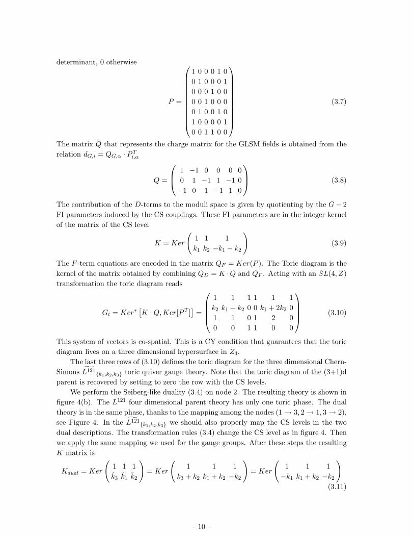
The matrix Q that represents the charge matrix for the GLSM fields is obtained from the

relation dG,i = QG,α · P Ti,α

Q =

1 −1 0 0 0 0

0 1 −1 1 −1 0

−1 0 1 −1 1 0

(3.8)

The contribution of the D-terms to the moduli space is given by quotienting by the G− 2

FI parameters induced by the CS couplings. These FI parameters are in the integer kernel

of the matrix of the CS level

K = Ker

(1 1 1

k1 k2 −k1 − k2

)(3.9)

The F -term equations are encoded in the matrix QF = Ker(P ). The Toric diagram is the

kernel of the matrix obtained by combining QD = K ·Q and QF . Acting with an SL(4, Z)

transformation the toric diagram reads

Gt = Ker∗[K · Q,Ker[P T ]

]=

1 1 1 1 1 1

k2 k1 + k2 0 0 k1 + 2k2 0

1 1 0 1 2 0

0 0 1 1 0 0

(3.10)

This system of vectors is co-spatial. This is a CY condition that guarantees that the toric

diagram lives on a three dimensional hypersurface in Z4.

The last three rows of (3.10) defines the toric diagram for the three dimensional Chern-

Simons L121{k1,k2,k3} toric quiver gauge theory. Note that the toric diagram of the (3+1)d

parent is recovered by setting to zero the row with the CS levels.

We perform the Seiberg-like duality (3.4) on node 2. The resulting theory is shown in

figure 4(b). The L121 four dimensional parent theory has only one toric phase. The dual

theory is in the same phase, thanks to the mapping among the nodes (1 → 3, 2 → 1, 3 → 2),

see Figure 4. In the L121{k1,k2,k3} we should also properly map the CS levels in the two

dual descriptions. The transformation rules (3.4) change the CS level as in figure 4. Then

we apply the same mapping we used for the gauge groups. After these steps the resulting

K matrix is

Kdual = Ker

(1 1 1

k3 k1 k2

)= Ker

(1 1 1

k3 + k2 k1 + k2 −k2

)= Ker

(1 1 1

−k1 k1 + k2 −k2

)

(3.11)

– 10 –

where with ki we denote the CS level of the i-th node in the dual phase. Concerning

the field content and the superpotential, the dual theory is in the same phase than the

starting theory. Thus we use the same matrices P, d,Q for the computation of the moduli

space. The toric diagram is then computed with the usual algorithm. Up to an SL(4, Z)

transformation it coincides with the same as the one computed in the original theory (3.10).

In this example we have shown that the Seiberg like duality (3.4) is a toric duality.

Observe that the non trivial transformation on the CS levels of (3.4) are necessary for the

equivalence of the moduli spaces of the two phases.

3.3 L222{ki}

The second example is the L222{ki} theory. The main difference is that this theory has

two phases with a different matter content and superpotential (see Figure 5), obtained by

dualizing node 2. These phases are dual for the (3+1)d parents theory. Here we show that

the same holds in three dimensions with the Seiberg like duality (3.4). The P, d,Q and K

N4,−k1−k2−k3

N1,k1+k2

N3,k2+k3

N4,−k1−k2−k3

N3,k3

N1,k1

N2,k2 N2+|k2|,−k2

Figure 5: The quivers for the two phases of L222.

matrices for the first phase are

d =

1 −1 0 0 0 0 −1 1

−1 1 1 −1 0 0 0 0

0 0 −1 1 1 −1 0 0

0 0 0 0 −1 1 1 −1

P =

0 0 0 0 1 0 1 0

0 0 0 0 0 1 0 1

1 0 1 0 0 0 0 0

0 1 0 1 0 0 0 0

0 0 0 0 1 1 0 0

0 0 0 0 0 0 1 1

1 1 0 0 0 0 0 0

0 0 1 1 0 0 0 0

(3.12)

Q =

−1 0 1 0 1 −1 0 0

1 −1 0 0 −1 1 0 0

−1 1 0 0 0 1 0 −1

1 0 −1 0 0 −1 0 1

K = Ker

(1 1 1 1

k1 k2 k3 −k1 − k2 − k3

)(3.13)

– 11 –

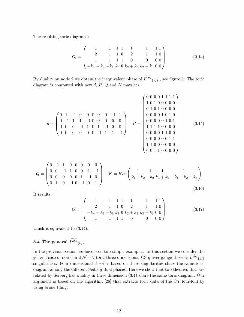
The resulting toric diagram is

Gt =

1 1 1 1 1 1 1 1

2 1 1 0 2 1 1 0

1 1 1 1 0 0 0 0

−k1 − k2 −k1 k2 0 k2 + k3 k2 + k3 0 0

(3.14)

By duality on node 2 we obtain the inequivalent phase of L222{ki} , see figure 5. The toric

diagram is computed with new d, P , Q and K matrices

d =

0 1 −1 0 0 0 0 0 −1 1

0 −1 1 1 −1 0 0 0 0 0

0 0 0 −1 1 0 1 −1 0 0

0 0 0 0 0 0 −1 1 1 −1

P =

0 0 0 0 1 1 1 1

1 0 1 0 0 0 0 0

0 1 0 1 0 0 0 0

0 0 0 0 1 0 1 0

0 0 0 0 0 1 0 1

1 1 1 1 0 0 0 0

0 0 0 0 1 1 0 0

0 0 0 0 0 0 1 1

1 1 0 0 0 0 0 0

0 0 1 1 0 0 0 0

(3.15)

Q =

0 −1 1 0 0 0 0 0

0 0 −1 1 0 0 1 −1

0 0 0 0 0 1 −1 0

0 1 0 −1 0 −1 0 1

K = Ker

(1 1 1 1

k1 + k2 −k2 k3 + k2 −k1 − k2 − k3

)

(3.16)

It results

Gt =

1 1 1 1 1 1 1 1

2 1 1 0 2 1 1 0

−k1 − k2 −k1 k2 0 k2 + k3 k2 + k3 0 0

1 1 1 1 0 0 0 0

(3.17)

which is equivalent to (3.14).

3.4 The general Laba{ki}

In the previous section we have seen two simple examples. In this section we consider the

generic case of non-chiral N = 2 toric three dimensional CS quiver gauge theories Laba{ki}

singularities. Four dimensional theories based on these singularities share the same toric

diagram among the different Seiberg dual phases. Here we show that two theories that are

related by Seiberg like duality in three dimension (3.4) share the same toric diagram. Our

argument is based on the algorithm [28] that extracts toric data of the CY four-fold by

using brane tiling.

– 12 –

Toric diagrams from bipartite graphs

Let us remind the reader that to every quiver describing a four dimensional conformal

field theory on D3 branes at Calabi Yau three-fold singularities it is possible to associate a

bipartite diagram drawn on a torus. It is called tiling or dimer [49, 50], and it encodes all

the informations in the quiver and in the superpotential. To every face in the dimer we can

associate a gauge group factor, to every edge a bifundamental field and to every node a term

in the superpotential. A similar tiling can be associated with three dimensional Chern-

Simons matter theories living on M2 branes probing a Calabi Yau four-fold singularity

simply adding a flux of Chern-Simons charge. The CS levels are described as a conserved

flow on the quiver, or equivalently on the dimer. To every edge we associate a flux of

Chern-Simons charge and the CS level of the gauge group is the sum of these contributions

taken with sign depending on the orientation of the arrow.

In this section we review the proposal of [28] for the computation of the moduli space

of three dimensional CS toric quiver gauge theories. This method furnishes the toric data

from the bipartite graphs associated with the quiver model and with the CS levels.

One has to choose a set of paths (p1, . . . , p4)on the dimer. The paths p1 and p2

correspond to the α and β cycles of the torus described by the dimer. The path p4 is a

paths encircling one of the vertices. One can also associate mesonic operators to these paths.

These operators correspond to the product of the corresponding bifundamentals along the

paths. For example the operator associated on the p4 path is a term of the superpotential.

The moduli space of the three dimensional theory requires also the definition of the path

p3. This is a product of paths corresponding to a closed flow of CS charges along the

quiver. We choose p3 in the tiling of the Laba singularity by taking a minimal closed path

connecting the bifundamentals from the first node to the a+ b-th node of the quiver. Then

one associates the CS chargen∑

i=1

ki (3.18)

to each bifundamental in this closed loop, with n = 1, . . . , a + b. The last charge is zero

since it corresponds to sum of all the CS levels in the theory. This conserved CS charges

flow is represented on the dimer by a set of oriented arrows connecting the faces of the

dimer, the gauge groups.

In [28] it has been shown that the toric polytope of CY4 is given by the convex hull of

all lattice point vα = (vα1 , . . . , vα

4 ), with

vαi = 〈pi,Dα〉 (3.19)

where Dα are the perfect matchings. The operation 〈., .〉 in (3.19) is the signed intersection

number of the perfect matching Dα with the path pi. Note that v4 is always 1, since there

is always only one perfect matching connected with the node encircled by p4.

Seiberg-like duality on Laba{ki} and toric duality

In subsection (3.1) we argued that the action of Seiberg duality on the field content and

on the superpotential is the same as in four dimensions. The only difference is the change

of the CS levels associated with the groups involved in the duality (3.4).

– 13 –

X23X12

X34

k1 k1+k2

k1+k2+k3

Y23Y12

−k1−k2 −k1

Figure 6: Action of Seiberg duality on the dimer and modification of the CS flow.

In an Laba theory, if duality is performed on node N2, the levels become

k1 → k1 + k2

k2 → −k2

k3 → k3 + k2 (3.20)

The action of Seiberg duality (3.4) not only modifies the dimer as in the 4d, but also the

CS levels of the gauge groups. This changes the path p3 in the dual description. Many

SL(4, Z) equivalent choices are possible. Among them we select the p3 path as in figure

6. We associate a charge l1 to Y12 and l2 to Y23, but with the opposite arrows that before.

The values of the charges l1 and l2 are derived from (3.20) and are

l1 = −k1 − k2 l2 = −k1 (3.21)

The field X34 is not involved in this duality and it contributes to the CS flow with the

same charge k1 + k2 + k3 in both phases.

We claim that the two theories share the same toric diagram. For the proof of this

relation it is useful to distinguish two sector of fields from which all the perfect matching

are built. In Figure 7 we separated these two sectors for the electric and magnetic phase

of an Laaa theory (the same distinction is possible in a generic Laba theory). Every perfect

matching is built by choosing in these sets only one field associated with each vertex. For

example in Figure 7(a) every perfect matching is a set of blue lines chosen such that every

vertex is involved only once.

The paths p1 and p2 are shown in figure 8 for the electric and the magnetic phase. The

intersection numbers 〈p1,Dα〉 and 〈p2,D

α〉 give the same bidimensional toric diagram of

the associated four dimensional Laba theories, up to an overall SL(3, Z) translation. This is

shown by mapping the perfect matching in the two description. This mapping is done with

– 14 –

(a) (b)

Figure 7: Different sectors of fields that generate all perfect matching in the (a) electric and (b)

magnetic theory

P4

(a)

P1

2P P

P

1

4

(b)P2

Figure 8: Paths pi in the two dual versions of the theory

a prescription on the choice of the fields in the perfect matching of the dual description. If

duality is performed on node Ni, the field Xi−1,i, Xi,i−1, Xi,i+1 and Xi+1,i are respectively

mapped in the fields Yi,i+1, Yi+1,i, Yi−1,i and Yi.i−1 of the dual theory. This prescription

gives a 1 − 1 map of each point of the 2d toric diagrams of the two dual theories.

The whole diagram for the three dimensional Laba theory is obtained by considering

the intersection numbers 〈p3,Dα〉, which give the third component of the vectors vα. The

path p3 corresponds to the flux of CS charges from the group N1 to the group Ng, where

the last arrow is omitted since it carries zero charge. In the dual theory the path p3 changes

as explained above, and as we show in Figure 8 for duality on a node labelled by 2. Note

that only the arrows connected with the dualized gauge group change.

With this choice of p3 and using the basis of perfect matching we prescribed, the

intersection numbers 〈p3,Dα〉 coincide in the two phases for every point of the 2d toric

diagram. This is shown by associating the relevant part of the path p3 to each sector of

perfect matching as in Figure 9. The arrow that carries charge k1 in the electric theory

corresponds to the arrow with charge −k1 in the magnetic theory. Its contribution to the

– 15 –

k1+k2

k1+k2+k3

k1+k2+k3+k4

.........

(a)

k1

k1+k2+k3+k4(b)

.....

k1+k2+k3 .....−k1−k2

−k1

Figure 9: Decomposition of the path p3 on the different perfect matchings

moduli space remains the same, since also the orientation of this arrow is the opposite.

The same happens for the arrow carrying charge k1 + k2.

Thus the 3d toric diagrams of the two dual theories are the same. We conclude that

the action of three dimensional Seiberg like duality (3.4) in the Laba{ki} theories implies

toric duality.

4. Chiral theories

In this section we study Seiberg like duality for N = 2 three dimensional Chern-Simons

theories with four dimensional parent chiral theories, which as such suffer from anomalies.

The anomaly free condition imposes constraints on the rank distribution. In 3d there are

no local gauge anomalies. Nevertheless we work with all U(N) gauge groups such that

the moduli space is the N symmetric product of the abelian one. Moreover for three

dimensional Chern-Simons chiral theories we do not have a brane construction as simple

as for the non-chiral case, and were not able to deduce the duality from the brane picture.

However, using what we learnt from the non-chiral case, we infer that at least a subset

of the possible three dimensional Seiberg-like toric dualities acts on the field content and

on the superpotential as it does in 4d and moreover recombines the Chern-Simons levels

in a similar way as in (3.4). As a matter of fact, a straightforward extension of the rule

(3.4) does not seem to work in the chiral case. This could be related to the fact that the

Master Spaces of the four dimensional dual Seiberg parents are not isomorphic [37]. For

this reason we restrict ourself to the case where the CS level of the group which undergoes

duality is set to zero. We assume that the other CS levels are unchanged, and no fractional

branes are created. This could be suggested by the parity anomaly matching argument

(see appendix A). We also set to zero the CS level of those gauge groups that after duality

have the same interactions with the rest of the quiver as the dualized gauge group.

– 16 –

By direct inspection we find that under these assumptions on the CS levels also for

chiral 3D CS theories Seiberg like duality leads to toric duality. For F0 we can take milder

assumptions. Indeed we find that a generalization of the rule (3.4) to the chiral case still

gives toric duality for this theory.

4.1 F0{ki}

Here we study the (2+1)d CS chiral theory whose (3+1)d parent is F0. In (3+1)d there are

two dual toric phases of F0, denoted as FI0 and FII

0 . In (2+1)d the two phases for arbitrary

choices of the CS levels do not have the same moduli space. Nevertheless it is possible to

find assignments for the Chern-Simons levels such that the two phases have the same toric

diagram.

(a) (b)

k1 k2

k3

−k2

−k1−k2−k3−k1−k2−k3

k1+k2

k2+k3

Figure 10: (a) quiver for FI0 and (b) quiver for FII

0 for one of the possible choice of CS levels.

The quiver representing the FI0 phase is in figure 10(a). The superpotential is

W = εijεklXi12X

k23X

j34X

l41 (4.1)

The incidence matrix and the matrix of perfect matchings are

d =

1 -1 0 0 0 0 -1 1

-1 1 1 -1 0 0 0 0

0 0 -1 1 1 -1 0 0

0 0 0 0 -1 1 1 -1

P =

1 1 0 0 0 0 0 0

1 0 1 0 0 0 0 0

0 0 0 0 1 1 0 0

0 0 0 0 1 0 1 0

0 1 0 1 0 0 0 0

0 0 1 1 0 0 0 0

0 0 0 0 0 1 0 1

0 0 0 0 0 0 1 1

(4.2)

– 17 –

The charges of the GLSM fields determine the matrix Q, the can be chosen as

Q =

1 0 0 0 0 0 0 -1

-1 0 0 0 1 0 0 0

0 0 0 1 -1 0 0 0

0 0 0 -1 0 0 0 1

(4.3)

The second phase FII0 is obtained by dualizing node 2. The dual superpotential is

W = εijεklXik13X

l32X

j21 − εijεklX

ik13X

l34X

j41 (4.4)

The matrices d, P and Q are determined from the quiver and the superpotential

d =

0

B

B

@

-1 -1 0 0 0 0 -1 -1 1 1 1 1

1 1 -1 -1 0 0 0 0 0 0 0 0

0 0 1 1 1 1 0 0 -1 -1 -1 -1

0 0 0 0 -1 -1 1 1 0 0 0 0

1

C

C

A

P =

0

B

B

B

B

B

B

B

B

B

B

B

B

B

B

B

B

B

B

B

@

0 0 0 0 0 1 0 1 1

0 0 1 0 0 1 0 0 1

0 0 0 1 1 0 1 0 0

0 1 0 0 1 0 1 0 0

0 0 1 0 0 0 1 0 1

0 0 0 0 0 0 1 1 1

0 1 0 0 1 1 0 0 0

0 0 0 1 1 1 0 0 0

1 1 1 0 0 0 0 0 0

1 1 0 0 0 0 0 1 0

1 0 0 1 0 0 0 1 0

1 0 1 1 0 0 0 0 0

1

C

C

C

C

C

C

C

C

C

C

C

C

C

C

C

C

C

C

C

A

(4.5)

Q =

1 0 0 0 0 -1 0 0 0

0 0 0 0 -1 1 0 0 0

-1 0 0 0 0 0 1 0 0

0 0 0 0 1 0 -1 0 0

(4.6)

Two families

The F0{ki} theories turn out to be a special case. Indeed one can single out two different

possibilities: in the first one we put to zero just the CS level associated with the group 2;

while in the second case we can fix to zero just the Chern-Simons level of the group 4 and

transform the CS levels as in the non-chiral case. In the first case we choose the CS levels

as (k1, k2, k3, k4) = (k, 0, p,−k − p). The CS level matrix for both phases is:

C =

(1 1 1 1

k 0 p −k − p

)(4.7)

and the toric diagram is given by:

G(I)t =

1 1 1 1 1 1 1 1

p 0 p 0 p p k+p k+p

0 1 -1 0 0 0 0 0

0 0 0 0 0 1 -1 0

(4.8)

The CS levels for the dual phase, obtained by duality on N2, are unchanged and the toric

diagram

G(II)t =

1 1 1 1 1 1 1 1 1

p k+p p p k+p k+p 0 0 0

0 0 -1 0 0 0 0 1 0

0 -1 0 1 0 0 0 0 0

(4.9)

– 18 –

is equivalent to the one above.

In the second case we choose the CS levels as (k1, k2, k3, k4) = (k, p,−k − p, 0). The

phase FII0 is computed by dualizing the node 2. We observe that by applying the rules

(3.4) the CS levels of FII0 are (k + p,−p,−k, 0). The C matrices for the two phases are:

CI =

(1 1 1 1

k p −k − p 0

)CII =

(1 1 1 1

k + p −p −k 0

)(4.10)

The toric diagram for the first phase is:

G(I)t =

1 1 1 1 1 1 1 1

k k 0 0 k+p 0 k+p 0

0 0 0 0 0 1 -1 0

0 -1 1 0 0 0 0 0

(4.11)

while the toric diagram for the second phase is:

G(II)t =

1 1 1 1 1 1 1 1 1

0 0 0 k k k+p k k+p k+p

0 0 1 0 0 0 0 -1 0

0 1 0 -1 0 0 0 0 0

(4.12)

And they are equivalent.

The F0 theory seems to be the only case where the assumptions we gave at the be-

ginning of this section can be relaxed. In the following examples we will just apply those

basic rules.

4.2 dP1{ki}

Here we study the (2+1)d CS chiral theory whose (3+1)d parent is dP1. In (3+1)d dP1 has

only one phase. After Seiberg duality on node 2 the theory has a self similar structure and

it is described by the same quiver. The only difference is that we have to change the labels

of the groups as (1 → 2, 2 → 4, 3 → 1, 4 → 3). The matrix d, P and Q are unchanged by

duality. The CS levels in the C matrix change as the labels of the gauge groups do. We

give in figure 11 the two phases.

We take the assumption described in the introduction of section 4. Hence we choose

the CS level of the group that undergoes duality to be 0. With this choice the two phases

of the 2 + 1 dimensional theory (see figure 11) have the same toric diagram.

The superpotential is

W = εabX13Xa34X

b41 + εabX42X

a23X

b34 + εabX34X

a41X12X

b23 (4.13)

The d, P,Q matrices are

d =

0

B

B

@

1 0 -1 0 0 0 -1 0 0 1

0 0 0 0 -1 1 0 1 0 -1

-1 1 0 1 0 -1 0 -1 1 0

0 -1 1 -1 1 0 1 0 -1 0

1

C

C

A

P =

0

B

B

B

B

B

B

B

B

B

B

B

B

B

B

@

1 1 1 0 0 0 0 0

0 0 0 1 1 1 0 0

0 0 0 0 0 0 1 1

0 0 0 1 1 0 1 0

1 1 0 0 0 0 0 1

0 0 1 0 0 1 0 0

0 0 0 0 0 1 0 1

0 0 1 0 0 0 1 0

1 0 0 1 0 0 0 0

0 1 0 0 1 0 0 0

1

C

C

C

C

C

C

C

C

C

C

C

C

C

C

A

(4.14)

– 19 –

−k1−k3 k3 k3 k1

k1 0 0 −k1−k31 2

34

4

13

2

Figure 11: Quiver and CS level for the dP1{ki} in the two phases related by duality on node 2.

Q =

0 0 1 0 1 -1 -1 0

0 -1 1 0 0 0 0 0

0 0 -1 1 0 0 0 0

0 1 -1 -1 -1 1 1 0

(4.15)

Following the relabeling of the gauge groups, the C matrix in the two phases are

C1 =

(1 1 1 1

k1 0 k3 −k1 − k3

)C2 =

(1 1 1 1

0 −k1 − k3 k1 k3

)(4.16)

The toric diagram for the first theory is given by the matrix G(1)t

G(1)t =

1 1 1 1 1 1 1 1

0 0 0 0 0 -1 1 0

-1 0 0 0 1 1 0 0

k1 + k3 k1 k1 k1 + k3 k1 k1 0 0

(4.17)

The toric diagram of the dual theory, up to SL(4, Z) transformation, is

G(2)t =

1 1 1 1 1 1 1 1

0 0 0 0 0 -1 1 0

-1 0 0 0 1 1 0 0

k1 + k3 k1 + k3 0 k1 k1 0 k1 k1 + k3

(4.18)

This shows that the two systems of vectors give the same toric diagram and that the two

theories have the same abelian moduli space also in the 2+ 1 dimensions, provided k2 = 0.

4.3 dP2{ki}

We analyze the (2+1)d CS chiral theory with dP2 as (3+1)d parents. The 4D theory

has two inequivalent phases. The two phases are connected by duality on node 5 and are

reported in figure 12.

The constraint on the CS levels explained in the introduction of this section imposes

k2 = 0 and k5 = 0. Under this assumption the two phases have the same toric diagram

also for the (2+1)d CS theory.

– 20 –

1

5

34

2

12

3

5

4

Figure 12: The quivers representing the dual phases of dP2

The superpotential for the two phases are

WI = X13X34X41 − Y12X24X41 + X12X24X45Y51 − X13X35Y51

+ Y12X23X35X51 − X12X23X34X45X51

WII = Y41X15X54 − X31X15X53 + Y12X23X31 − Y12X24X41 + Y15X53X34X41

− Z41Y15X54 + X12X24Z41 − X12X23X34Y41 (4.19)

We compute the toric diagrams G(I)t and G

(II)t for the two phases

G(I)t =

1 1 1 1 1 1 1 1 1 1

0 0 1 0 0 0 0 -1 0 -1

0 -1 0 0 1 0 0 0 0 -1

k1 k1 k1 k1 0 0 0 0 −k3 −k3

G(II)t =

1 1 1 1 1 1 1 1 1 1 1

0 -1 0 0 1 0 0 0 0 0 -1

0 -1 -1 0 0 0 0 1 0 0 0

0 −k3 k1 0 k1 −k3 k1 0 0 0 0

(4.20)

They result the same.

4.4 dP3{ki}

Here we study dP3{ki}. This theory has four phases in four dimensions, with superpotentials

WI = X13X34X46X61 − X24X46X62 + X12X24X45X51 − X13X35X51

+ X23X35X56X62 − X12X23X34X45X56X61

WII = X13X34X41 − X13X35X51 + X23X35X52 − X26X65X52 + X16X65Y51

− X16X64X41 + X12X26X64X45X51 − X12X23X34X45Y51

WIII = X23X35X52 − X26X65X52 + X14X46X65Y51 − X12X23Y35Y51 + X43Y35X54

− Y65X54X46 + X12X26Y65X51 − X14X43X35X51

– 21 –

WIV = X23X35X52 − X52X26X65 + X65Z54X46 − Z54X41Y15 + Y15Z52X21 − Z52X23Y35

+ Y35X54X43 − X54X46Y65 + Y65Y52X26 − Y52X21X15 + X15Y54X41 − Y54X43X35

Phases (II, III, IV) are computed from phases (I, II, III) by dualizing nodes (6, 4, 1)respectively. The quivers associated with each phase are given in Figure 13. We now

21

45

63

1

2

5

34 6

1

4

5

2

6

5

3 142

I

IV

II

III

63

Figure 13: The quiver of dP3

show the equivalence of phases (I,II), (II,III) and (III,IV) by choosing (k3 = k6 = 0),(k2 = k4 = 0) and (k1 = k3 = k6 = 0) respectively. For phases (I, II) we have

G(I)t

=

0

B

B

@

1 1 1 1 1 1 1 1 1 1 1 1

-1 0 0 0 0 1 0 0 0 -1 1 0

-1 0 -1 0 0 1 0 1 0 0 0 0

k1 + k2 0 k1 k1 + k2 + k4 k1 + k2 0 k1 k1 + k2 + k4 k1 + k2 k1 + k2 0 0

1

C

C

A

G(II)t

=

0

B

B

@

1 1 1 1 1 1 1 1 1 1 1 1 1

0 0 -1 0 0 0 0 -1 0 0 0 1 1

0 1 0 0 0 -1 0 -1 0 0 0 0 1

k1 k1 + k2 + k4 k1 + k2 k1 + k2 k1 + k2 k1 k1 + k2 + k4 k1 + k2 k1 + k2 k1 + k2 0 0 0

1

C

C

A

For phases (II, III) we have

G(II)t

=

0

B

B

@

1 1 1 1 1 1 1 1 1 1 1 1 1

0 1 1 0 0 -1 0 0 0 0 0 -1 0

0 0 1 0 0 0 0 1 0 0 0 -1 -1

−k1 k3 + k5 k3 + k5 k3 + k5 −k1 −k1 − k3 k5 −k1 − k3 k5 −k1 − k3 0 0 0

1

C

C

A

G(III)t

=

0

B

B

@

1 1 1 1 1 1 1 1 1 1 1 1 1 1

0 1 0 0 1 0 -1 0 0 -1 0 0 0 0

0 1 -1 0 0 0 -1 0 0 0 0 0 1 0

0 k3 + k5 0 −k1 k3 + k5 −k1 0 k3 + k5 k5 −k1 − k3 −k1 −k1 −k1 − k3 −k1 − k3

1

C

C

A

For phases (III, IV ) we have

G(III)t

=

0

B

B

@

1 1 1 1 1 1 1 1 1 1 1 1 1 1

0 -1 1 0 0 0 1 0 0 0 0 0 -1 0

0 -1 0 0 -1 0 1 0 0 1 0 0 0 0

k2 + k4 k2 k2 + k4 k2 k2 + k4 k2 + k4 k4 0 0 0 0 k4 0 0

1

C

C

A

G(IV )t

=

0

B

B

@

1 1 1 1 1 1 1 1 1 1 1 1 1 1 1 1 1

0 0 0 0 1 0 0 0 0 0 0 1 0 -1 0 0 -1

0 0 0 0 0 -1 0 0 0 0 0 1 0 -1 1 0 0

k2 + k4 k2 + k4 k2 + k4 k2 + k4 k2 + k4 k2 + k4 k2 + k4 k2 + k4 k2 + k4 k2 + k4 k4 k4 k2 k2 0 0 0

1

C

C

A

– 22 –

4.5 Y 32{ki}

This is the last chiral theory we analyze. In this case, after duality, there is not an identi-

fication between the gauge group that undergoes duality with other groups. This implies

that the assumptions of section 4 impose only kg = 0, where kg is the CS level of the

dualized gauge group. As for the case of dP1 and all the Y p,p−1 theories, the Y 3,2 theory

is self similar under four dimensional Seiberg duality. We can evaluate M4 for one phase

and then the toric diagram associated with a dual phase is given by an appropriate change

of the D-term modding matrix.

We fix the conventions on the groups by giving the tiling of the two dual phases, see

Figure 14. The two phases are connected by duality on node 5, so we set k5 = 0.

2

3

4

6

1

5

3

4

2

1

4

56

1

2

3

53

2

4

6

1 53

2

4

6

1

4

6

1

2

Figure 14: The tiling for the two dual phases of Y 32. Seiberg duality has been performed on

groups 5.

The CS matrices for the two dual phases are:

C1 =

1 1 1 1 1 1

k1 k2 k3 k4 0 −k1 − k2 − k3 − k4

!

C2 =

1 1 1 1 1 1

k4 −k1 − k2 − k3 − k4 k1 k2 k3 0

!

The toric diagrams are encoded in the Gt matrices.

G(1)t

=

0

B

B

@

1 1 1 1 1 1 1 1 1 1 1 1 1 1 1 1 1 1

0 0 0 0 0 0 0 0 0 0 0 0 1 0 0 0 0 -1

2 1 1 1 0 1 0 0 1 0 0 0 -1 -1 1 0 0 0

k3 + k4 0 −k6 k2 + k3 + k4 k2 k3 + k4 0 −k6 k4 −k3 k1 + k2 + k4 k2 + k4 k1 + 2k2 + k4 k2 − k3 0 k2 0 0

1

C

C

A

G(2)t

=

0

B

B

@

1 1 1 1 1 1 1 1 1 1 1 1 1 1 1 1 1 1

0 0 0 0 0 0 0 0 0 0 0 0 1 0 0 0 0 -1

2 1 1 1 0 1 0 0 1 0 0 0 -1 -1 1 0 0 0

k3 + k4 k4 k4 0 −k3 −k6 k1 + k2 + k4 k1 + k2 + k3 k2 + k3 + k4 k2 + k4 k2 + k4 k2 k1 + 2k2 + k4 k2 − k3 k3 + k4 0 −k6 0

1

C

C

A

and they coincide for arbitrary k1, k2, k3, k4, remind k6 = −k1 − k2 − k3 − k4.

5. Dualities for CS theories without 4d parents

Three dimensional CS theories with four dimensional parents are a subset of all the possible

3d CS theories [27]. For CS theories without four dimensional parents we miss in principle

– 23 –

the intuition from the 4d Seiberg duality. In this short section we see that we can still

describe a subset of 3d CS theories with the same mesonic moduli space if we just apply

the rules we learnt in the previous sections.

We study a case associated with Q111. We show that by performing a Seiberg-like

duality and by setting the CS level of the dualized gauge group to zero, the toric diagrams

of the two models coincide.

(a) (b)

k1 k2

−k1−k2

0

k1

−k1−k2

k2

0

Figure 15: The quiver for Q111 in the two dual phases.

5.1 Example

The theory is described by the quiver given in Figure 15a. It is a generalization of the

C(Q1,1,1) with arbitrary CS levels [27]. The superpotential is

W = X41X13X134X42X23X

234 − X41X13X

234X42X23X

134 (5.1)

The toric diagram for k4 = 0 is given by

Gt =

1 1 1 1 1 1

1 0 1 0 1 0

1 0 0 1 1 0

k1 k2 0 0 0 0

(5.2)

Seiberg duality on node N4 gives the superpotential

W = X13X(1)32 X23X

(2)31 − X13X

(2)32 X23X

(1)31 + X24X

(2)43 X

(2)32 − X24X

(1)43 X

(1)32

+ X14X(1)43 X

(1)31 − X14X

(2)43 X

(2)31 (5.3)

– 24 –

and the theory is described by the quiver given in Figure 15b. The toric diagram in this

case is

Gt =

1 1 1 1 1 1 1 1

1 0 1 0 1 0 1 0

1 0 1 0 1 1 0 0

k1 k2 k1 k2 0 0 0 0

(5.4)

and it is equivalent to the toric diagram for the first phase.

6. Conclusion

In this paper we have some advances towards the understanding of toric duality for M2

branes. Generalizing the work of [32, 31], we proposed a Seiberg-like duality for non-chiral

three dimensional CS matter theories and we verified that the mesonic moduli space of dual

theories is indeed the same four-fold Calabi Yau probed by the M2 branes. In the chiral

case and in the case in which the three dimensional theories do not have a four dimensional

parent, the situation is more complicated. However, fixing to zero the value of some of the

Chern-Simons levels, we were able to realize toric dual pairs.

We have just analyzed the mesonic moduli space, it would be important to study the

complete moduli space, including baryonic operators.

For the non-chiral case the two main limitations are the lack of understanding of the

transformation rule for the rank of the gauge groups and the fact that we forced to zero some

of the ki. It is reasonable that there exist some more general and precise transformation

rules and we would like to investigate them.

We concentrated on Seiberg-like transformations, but it is well known that in three

dimension there exist duality maps that change the number of gauge group factors. It

would be interesting to systematically study these more general transformations.

A lot of possible directions and generalizations are opening up and after these first

steps we hope to step up.

Acknowledgments

We are happy to thank Alberto Zaffaroni for many nice discussions and Ami Hanany for

comments. We are grateful to the authors of [54, 55] for informing us about their research

on similar topics.

A. A. and L. G. are supported in part by INFN, in part by MIUR under contract

2007-5ATT78-002 and in part by the European Commission RTN programme MRTN-CT-

2004-005104. D. F. is supported by CNRS and ENS Paris. A. M. is supported in part

by the Belgian Federal Science Policy Office through the Interuniversity Attraction Pole

IAP VI/11, by the European Commission FP6 RTN programme MRTN-CT-2004-005104

and by FWO-Vlaanderen through project G.0428.06.

– 25 –

A. Parity anomaly

We briefly review parity anomaly for 3D gauge theories [51, 52] and the parity anomaly

matching agument [33]. In three dimensions there are no local gauge anomalies. However

gauge invariance can require the introduction of a classical Chern-Simons term, which

breaks parity. This is referred to as parity anomaly.

For abelian theories with multiple U(1)’s, there is a parity anomaly if

Aij =1

2

∑

fermion

(qf )i(qf )j ∈ Z +1

2(A.1)

Here (qf )i is the charge of the fermion f under the U(1)i. We work in a basis where all

the charges are integers.

Parity anomaly matching

In the context of dualities in 4D gauge theory, a relevant tool have been the t’Hooft

anomaly matching between the electric and the magnetic description. Having some global

symmetries, we suppose that they are gauged and we compute their anomaly. The result

of this computation should be equal in the two dual descriptions. The same technique can

be used here for the parity anomaly. We suppose we gauge the global U(1)’s of the theory,

and we compute their parity anomaly both in the electric and in the magnetic description.

The two computations should match.

The parity anomaly matching is much weaker then the t’Hooft one. Indeed in 4D the

precise anomalies associated with gauging global symmetries must match. In 3D there is

a weaker Z2 type condition.

For the Laba{ki} theories, parity anomaly matching is obeyed by the Seiberg like duality

we propose.

In chiral theories, parity anomaly matching can be non trivial between dual phases if

fractional branes are introduced by the duality.

As an example we analyze the toric chiral (2+1)d CS theory which has as (3+1)d

parents dP2. We consider the parity anomaly associated to the two U(1) flavour symmetries

F1 and F2. The charges of the chiral fields of the theory under these symmetries can be

derived from [37]. The electric theory has equal ranks n. In the magnetic description we

set rank n + k for the dualized gauge group (number 5) and n for the others. The integer

k counts the number of fractional branes introduced in the duality. The parity anomaly

matrices are

Aele ∈

(Z Z

Z Z

)(A.2)

and

Amag ∈

(Z Z + nk

2

Z + nk2 Z

)(A.3)

One can see that in the electric description there are no parity anomalies. In the magnetic

description the off diagonal components of Amag can instead lead to parity anomaly if kn

– 26 –

is odd. If we set k = 0 the electric and magnetic theories satisfies the parity anomaly

matching for the two flavour symmetries.

References

[1] B. Feng, A. Hanany and Y. H. He, “D-brane gauge theories from toric singularities and toric

duality,” Nucl. Phys. B 595, 165 (2001) [arXiv:hep-th/0003085].

[2] B. Feng, A. Hanany and Y. H. He, “Phase structure of D-brane gauge theories and toric

duality,” JHEP 0108, 040 (2001) [arXiv:hep-th/0104259].

[3] B. Feng, S. Franco, A. Hanany and Y. H. He, “Symmetries of toric duality,” JHEP 0212, 076

(2002) [arXiv:hep-th/0205144].

[4] C. E. Beasley and M. R. Plesser, “Toric duality is Seiberg duality,” JHEP 0112, 001 (2001)

[arXiv:hep-th/0109053].

[5] B. Feng, A. Hanany, Y. H. He and A. M. Uranga, “Toric duality as Seiberg duality and brane

diamonds,” JHEP 0112, 035 (2001) [arXiv:hep-th/0109063].

[6] J. H. Schwarz, “Superconformal Chern-Simons theories,” JHEP 0411 (2004) 078

[arXiv:hep-th/0411077].

[7] J. Bagger and N. Lambert, “Modeling multiple M2’s,” Phys. Rev. D 75, 045020 (2007)

[arXiv:hep-th/0611108].

[8] J. Bagger and N. Lambert, “Gauge Symmetry and Supersymmetry of Multiple M2-Branes,”

Phys. Rev. D 77 (2008) 065008 [arXiv:0711.0955 [hep-th]].

[9] J. Bagger and N. Lambert, “Comments On Multiple M2-branes,” JHEP 0802, 105 (2008)

[arXiv:0712.3738 [hep-th]].

[10] A. Gustavsson, “Algebraic structures on parallel M2-branes,” Nucl. Phys. B 811, 66 (2009)

[arXiv:0709.1260 [hep-th]].

[11] A. Gustavsson, “Selfdual strings and loop space Nahm equations,” JHEP 0804, 083 (2008)

[arXiv:0802.3456 [hep-th]].

[12] M. Van Raamsdonk, “Comments on the Bagger-Lambert theory and multiple M2-branes,”

arXiv:0803.3803 [hep-th].

[13] S. Mukhi and C. Papageorgakis, “M2 to D2,” JHEP 0805, 085 (2008) [arXiv:0803.3218

[hep-th]].

[14] O. Aharony, O. Bergman, D. L. Jafferis and J. Maldacena, “N=6 superconformal

Chern-Simons-matter theories, M2-branes and their gravity duals,” JHEP 0810, 091 (2008)

[arXiv:0806.1218 [hep-th]].

[15] M. Benna, I. Klebanov, T. Klose and M. Smedback, “Superconformal Chern-Simons Theories

and AdS4/CFT3 Correspondence,” JHEP 0809, 072 (2008) [arXiv:0806.1519 [hep-th]].

[16] K. Hosomichi, K. M. Lee, S. Lee, S. Lee and J. Park, “N=4 Superconformal Chern-Simons

Theories with Hyper and Twisted Hyper Multiplets,” arXiv:0805.3662 [hep-th].

[17] K. Hosomichi, K. M. Lee, S. Lee, S. Lee and J. Park, “N=5,6 Superconformal Chern-Simons

Theories and M2-branes on Orbifolds,” JHEP 0809, 002 (2008) [arXiv:0806.4977 [hep-th]].

– 27 –

[18] M. Schnabl and Y. Tachikawa, “ Classification of N = 6 superconformal theories of ABJM

type,” arXiv:0807.1102 [hep-th].

[19] D. Martelli and J. Sparks, “Moduli spaces of Chern-Simons quiver gauge theories and

AdS(4)/CFT(3),” Phys. Rev. D 78, 126005 (2008) [arXiv:0808.0912 [hep-th]].

[20] A. Hanany and A. Zaffaroni, “Tilings, Chern-Simons Theories and M2 Branes,” JHEP 0810,

111 (2008) [arXiv:0808.1244 [hep-th]].

[21] A. Hanany, D. Vegh and A. Zaffaroni, “Brane Tilings and M2 Branes,” arXiv:0809.1440

[hep-th].

[22] D. L. Jafferis and A. Tomasiello, “A simple class of N=3 gauge/gravity duals,” JHEP 0810

(2008) 101 [arXiv:0808.0864 [hep-th]].

[23] D. Gaiotto and A. Tomasiello, “The gauge dual of Romans mass,” arXiv:0901.0969 [hep-th].

[24] Y. Imamura and K. Kimura, “On the moduli space of elliptic Maxwell-Chern-Simons

theories,” Prog. Theor. Phys. 120 (2008) 509 [arXiv:0806.3727 [hep-th]]; Y. Imamura and K.

Kimura, “N=4 Chern-Simons theories with auxiliary vector multiplets,” arXiv:0807.2144

[hep-th].

[25] Y. Imamura and S. Yokoyama, “N=4 Chern-Simons theories and wrapped M5-branes in their

gravity duals,” arXiv:0812.1331 [hep-th].

[26] A. Hanany and Y. H. He, “M2-Branes and Quiver Chern-Simons: A Taxonomic Study,”

arXiv:0811.4044 [hep-th].

[27] S. Franco, A. Hanany, J. Park and D. Rodriguez-Gomez, “Towards M2-brane Theories for

Generic Toric Singularities,” JHEP 0812 (2008) 110 [arXiv:0809.3237 [hep-th]].

[28] K. Ueda and M. Yamazaki, “Toric Calabi-Yau four-folds dual to Chern-Simons-matter

theories,” JHEP 0812, 045 (2008) [arXiv:0808.3768 [hep-th]].

[29] Y. Imamura and K. Kimura, “Quiver Chern-Simons theories and crystals,” JHEP 0810, 114

(2008) [arXiv:0808.4155 [hep-th]].

[30] A. Kapustin and M. J. Strassler, “On Mirror Symmetry in Three Dimensional Abelian Gauge

Theories,” JHEP 9904, 021 (1999) [arXiv:hep-th/9902033].

K. A. Intriligator and N. Seiberg, “Mirror symmetry in three dimensional gauge theories,”

Phys. Lett. B 387, 513 (1996) [arXiv:hep-th/9607207].

[31] O. Aharony, O. Bergman and D. L. Jafferis, “Fractional M2-branes,” JHEP 0811 (2008) 043

[arXiv:0807.4924 [hep-th]].

[32] A. Giveon and D. Kutasov, “Seiberg Duality in Chern-Simons Theory,” Nucl. Phys. B 812

(2009) 1 [arXiv:0808.0360 [hep-th]].

[33] O. Aharony, A. Hanany, K. A. Intriligator, N. Seiberg and M. J. Strassler, “Aspects of N = 2

supersymmetric gauge theories in three dimensions,” Nucl. Phys. B 499, 67 (1997)

[arXiv:hep-th/9703110].

[34] A. Karch, “Seiberg duality in three dimensions,” Phys. Lett. B 405 (1997) 79

[arXiv:hep-th/9703172].

O. Aharony, “IR duality in d = 3 N = 2 supersymmetric USp(2N(c)) and U(N(c)) gauge

Phys. Lett. B 404 (1997) 71 [arXiv:hep-th/9703215].

– 28 –

[35] D. Forcella, A. Hanany, Y. H. He and A. Zaffaroni, “The Master Space of N=1 Gauge

Theories,” JHEP 0808 (2008) 012 [arXiv:0801.1585 [hep-th]].

[36] D. Forcella, A. Hanany, Y. H. He and A. Zaffaroni, “Mastering the Master Space,” Lett.

Math. Phys. 85 (2008) 163 [arXiv:0801.3477 [hep-th]].

[37] D. Forcella, A. Hanany and A. Zaffaroni, “Master Space, Hilbert Series and Seiberg Duality,”

arXiv:0810.4519 [hep-th].

[38] S. Benvenuti and M. Kruczenski, “From Sasaki-Einstein spaces to quivers via BPS geodesics:

Lpqr,” JHEP 0604 (2006) 033 [arXiv:hep-th/0505206].

[39] A. Butti, D. Forcella and A. Zaffaroni, “The dual superconformal theory for L(p,q,r)

manifolds,” JHEP 0509 (2005) 018 [arXiv:hep-th/0505220].

[40] S. Franco, A. Hanany, D. Martelli, J. Sparks, D. Vegh and B. Wecht, “Gauge theories from

toric geometry and brane tilings,” JHEP 0601 (2006) 128 [arXiv:hep-th/0505211].

[41] A. Hanany and E. Witten, “Type IIB superstrings, BPS monopoles, and three-dimensional

gauge dynamics,” Nucl. Phys. B 492 (1997) 152 [arXiv:hep-th/9611230].

[42] T. Kitao, K. Ohta and N. Ohta, “Three-dimensional gauge dynamics from brane

configurations with (p,q)-fivebrane,” Nucl. Phys. B 539, 79 (1999) [arXiv:hep-th/9808111].

[43] O. Bergman, A. Hanany, A. Karch and B. Kol, “Branes and supersymmetry breaking in 3D

gauge theories,” JHEP 9910, 036 (1999) [arXiv:hep-th/9908075].

[44] A. M. Uranga, “Brane Configurations for Branes at Conifolds,” JHEP 9901 (1999) 022

[arXiv:hep-th/9811004].

[45] S. Elitzur, A. Giveon and D. Kutasov, Phys. Lett. B 400 (1997) 269 [arXiv:hep-th/9702014].

[46] V. Niarchos, “Seiberg Duality in Chern-Simons Theories with Fundamental and Adjoint

Matter,” JHEP 0811 (2008) 001 [arXiv:0808.2771 [hep-th]].

[47] E. Witten, “Supersymmetric index of three-dimensional gauge theory,”

arXiv:hep-th/9903005.

[48] K. Ohta, “Supersymmetric index and s-rule for type IIB branes,” JHEP 9910 (1999) 006

[arXiv:hep-th/9908120].

[49] A. Hanany and K. D. Kennaway, “Dimer models and toric diagrams,” arXiv:hep-th/0503149.

[50] S. Franco, A. Hanany, K. D. Kennaway, D. Vegh and B. Wecht, “Brane Dimers and Quiver

Gauge Theories,” JHEP 0601, 096 (2006) [arXiv:hep-th/0504110].

[51] L. Alvarez-Gaume and E. Witten, “Gravitational Anomalies,” Nucl. Phys. B 234, 269 (1984).

[52] A. N. Redlich, “Parity Violation And Gauge Noninvariance Of The Effective Gauge Field

Action In Three-Dimensions,” Phys. Rev. D 29, 2366 (1984).

[53] S. Kim, S. Lee, S. Lee and J. Park, “Abelian Gauge Theory on M2-brane and Toric Duality,”

Nucl. Phys. B 797, 340 (2008) [arXiv:0705.3540 [hep-th]].

[54] S. Franco, I. Klebanov and D. Rodriguez-Gomez, “M2-branes on Orbifolds of the Cone over

Q1,1,1,” arXiv:0903.3231 [hep-th].

[55] J. Davey, A. Hanany, N. Mekareeya and G. Torri, “Phases of M2-brane Theories,”

arXiv:0903.3234 [hep-th].

– 29 –