arX

iv:0

803.

1277

v3 [

hep-

th]

11

May

200

9

hep-th/yymmnnnILL-(TH)-08-xx

Transversely-intersecting D-branes at finite temperatureand chiral phase transition

Mohammad Edalati, Robert G. Leigh and Nam Nguyen Hoang

Department of Physics, University of Illinois at Urbana-Champaign, Urbana IL 61801, USA

edalati, rgleigh, nnguyen2@uiuc.edu,

Abstract

We consider Sakai-Sugimoto like models consisting of Dq-Dp-Dp-branes where Nf flavor Dp andDp-branes transversely intersect Nc color Dq-branes along two (r + 1)-dimensional subspaces. Forsome values of p and q, the theory of intersections dynamically breaks non-Abelian chiral symmetrywhich is holographically realized as a smooth connection of the flavor branes at some point in thebulk of the geometry created by Nc Dq-branes. We analyze the system at finite temperature andmap out different phases of the theory representing chiral symmetry breaking and restoration.For q ≤ 4 we find that, unlike the zero-temperature case, there exist two branches of smoothly-connected solutions for the flavor branes, one getting very close to the horizon of the backgroundand the other staying farther away from it. At low temperatures, the solution which stays fartheraway from the horizon determines the vacuum. For background D5 and D6-branes we find thatthe flavor branes, like the zero temperature case, show subtle behavior whose dual gauge theoryinterpretation is not clear. We conclude with some comments on how chiral phase transition inthese models can be seen from their open string tachyon dynamics.

1 Introduction, summary and conclusions

A very interesting holographic model of QCD which realizes dynamical breaking of non-Abelianchiral symmetry in a nice geometrical way is the Sakai-Sugimoto model [1]. In this model, one startswith Nc D4-branes extended in (x0x1x2x3x4)-directions with x4 being a circle of radius R. The lowenergy theory on the branes is a (4 + 1)-dimensional SU(Nc) SYM with sixteen supercharges. Tobreak supersymmetry, anti-periodic boundary condition for fermions around the x4-circle must bechosen. To this system, Nf D8 and Nf D8-branes are added such that they intersect the D4-branesat two (3 + 1)-dimensional subspaces R

3,1, and are separated in the compact x4-direction by acoordinate distance of ℓ0 = πR. In other words, the D8 and D8-branes are located asymptoticallyat the antipodal points on the circle. The massless degrees of freedom of the system are thegauge bosons coming from 4 − 4 strings and chiral fermions coming from 4-8 strings. (Beforecompactifying x4, there are also massless adjoint scalars and fermions coming from the 4 − 4strings. These modes become massive upon compactifying x4 and choosing anti-periodic boundarycondition for the adjoint fermions; fermions get masses at tree level whereas scalars get masses dueto loop effects.) The fermions localized at the intersection of D4 and D8-branes have (by definition)left-handed chirality and the fermions at the intersection of D4 and D8-branes are right-handed.The U(Nf) × U(Nf) gauge symmetry of the D8 and D8-branes in this model is interpreted as thechiral symmetry of the fermions living at the intersections. At weak effective four-dimensional ’tHooft coupling λ4 the low energy theory contains QCD but this is not the limit amenable to analysisby the gauge-gravity duality. At strong-coupling (λ4 ≫ 1), however, the theory is not QCD butcan be analyzed using the gauge-gravity duality [2, 3, 4, 5], and it has been suggested that it isin the same universality class as QCD. In lack of any rigorous proof for this universality, the bestone can do is to check whether this model at large Nc and large four-dimensional ’t Hooft couplingexhibits the key features of QCD; namely, confinement and spontaneous chiral symmetry breaking.In fact, it apparently does [1]. By considering Nf D8 and Nf D8-branes as probe “flavor” branesin the near-horizon geometry of Nc “color” D4-branes and analyzing the Dirac-Born-Infeld (DBI)action of the flavor branes in the background, one observes that at some radial point in the bulk thepreferred configuration of the flavor branes is that of smoothly-connected D8 and D8-branes. Thisgeometrical picture is interpreted as dynamical breaking of U(Nf)×U(Nf) chiral symmetry (wherethe branes are asymptotically separated) down to a single U(Nf) (where the branes connect). Themodel also shows confinement [6, 7].

Although choosing ℓ0 = πR makes calculations a bit simpler, there is no particular reason toconsider the flavor branes to be asymptotically located at the antipodal points of x4. In fact, theℓ0 ≪ πR limit of the Sakai-Sugimoto model is very interesting in its own right. By analyzing theℓ0 ≪ πR limit, or equivalently the R → ∞ limit, it was realized in [8] that the theory at theintersections can be analyzed both at weak and strong effective four-dimensional ’t Hooft couplingλ4. At weak-coupling the model can be analyzed using field theoretic methods and in fact is a non-local version of Nambu-Jona-Lasinio (NJL) model [9]. At strong-coupling it can be analyzed bystudying the DBI action of the flavor branes in the near-horizon geometry of the color branes andexhibits chiral symmetry breaking via a smooth fusion of the flavor branes at some (radial) point inthe bulk. A nice feature of this model is that the scale of chiral symmetry breaking is different fromthat of confinement [8], and one can completely turn off confinement by taking the R → ∞ limit.Therefore the ℓ0 ≪ πR limit of the Sakai-Sugimoto model provides a clean holographic model ofjust chiral symmetry breaking without complications due to confinement.

2

The finite-temperature analysis (at large Nc and large ’t Hooft coupling λ4) of the Sakai-Sugimoto model as well as the holographic NJL model [8], was carried out in [10, 11]. Putting theflavor branes as probes (Nf ≪ Nc) in the near-horizon geometry of Nc non-extremal D4-branes andanalyzing the DBI action of the flavor branes, one obtains [10, 11] that at low temperatures (com-pared to ℓ−1

0 ) the energetically-favorable solution is that of smoothly-connected D8 and D8-braneswhich, like its zero-temperature counterpart, is a realization of chiral symmetry breaking. At highenough temperatures, on the other hand, the preferred (in the path integral sense) configuration isthat of disjoint D8 and D8-branes, hence chiral symmetry is restored. Also, when x4 is compactand ℓ0 < πR, there exists an intermediate phase where the dual gauge theory is deconfined whilechiral symmetry is broken [10].

It is certainly interesting to explore whether the holographic realization of chiral symmetrybreaking and restoration is specific to a particular model such as the aforementioned ones, or genericin the sense that other intersecting brane models will realize it, too. To search for genericness (ornon-genericness) of chiral symmetry breaking in intersecting brane models, a system of Dq-Dp-Dp-branes was considered at zero temperature in [12] where the color Dq-branes are stretchedin non-compact (x0x1 . . . xq)-directions. The flavor Dp and Dp-branes intersect the color branesat two (r + 1)-dimensional subspaces R

r,1. Without flavor branes, the low energy theory on thecolor branes and whether it can be decoupled from gravity (or other non-field theoretic degreesof freedom) with an appropriate scaling limit was analyzed in [13]. The low energy theory on theDq-branes is asymptotically free for q < 3, conformal for q = 3, and infrared free for q > 3. Whilefor q ≤ 5, there always exists a scaling limit for which the open string modes can be decoupled fromthe closed string modes, there exists no such limit for q = 6. With the flavor branes present, ananalysis was carried out in [12] where the behavior of the model for both small and large effective’t Hooft coupling λeff ∼ λq+1ℓ

3−q0 (ℓ0 is the asymptotic coordinate distance between Dp and Dp-

branes, and λq+1 is the ’t Hooft coupling of the (q + 1)-dimensional theory on the Dq-branes.) wasconsidered. Taking the Nc → ∞ limit while keeping λeff fixed and large, amounts, in the probeapproximation, to putting the flavor branes in the near-horizon geometry of Nc color branes. (See[12, 13] for the validity of the supergravity analysis in these models.) Determining the shape ofthe flavor branes (relevant for chiral symmetry breaking) by analyzing their DBI action in thebackground geometry, it was observed that [12] for q ≤ 4 there always exists a smoothly-connectedbrane solution which is energetically favorable. For a subclass of these general intersecting branemodels, namely those for which q + p − r = 9, the above-mentioned connected solutions can beidentified with the U(Nf) × U(Nf) chiral symmetry being spontaneously broken. Following [12]we will call the brane models for which q + p − r = 9 as transversely-intersecting brane modelsand their intersections as transverse intersections. For q = 5, there exists no connected solutionexcept when ℓ0 takes a particular value. For this particular value of ℓ0 which is around the scaleof non-locality of the low energy theory on the D5-branes (which is a little string theory; see [14]for a review of little string theories), there is a continuum of connected solutions whose turningpoints can be anywhere in the radial coordinate of the bulk geometry. All such solutions are equallyenergetically favorable. For q = 6, there is a connected solution but is not the preferred one. Themore energetically favorable solution, in this case, is that of disjoint branes. Due to the lacking ofan appropriate decoupling limit for q = 6, it is not clear whether one can realize such a solution asa phase for which chiral symmetry is unbroken.

3

Summary and conclusions The purpose of this paper is to investigate some aspects of non-compact transversely-intersecting D-brane models at finite temperature, in particular the numberof solutions, their behavior, and whether or not such solutions can be identified with a chirallybroken (or restored) phase of the dual gauge theory living at the intersections. The main reasonfor us to consider transverse intersections is that in the probe approximation the generalizationof the Abelian U(1) × U(1) chiral symmetry to the non-Abelian case is straightforward: one justreplaces Nf = 1 with general Nf , and multiplies the flavor DBI action by Nf . This is not thecase in other holographic models of chiral symmetry breaking and restoration1. Note that theSakai-Sugimoto model [1], its non-compact version [8], and the D2-D8-D8 model analyzed in [17]which holographically realizes a non-local version of the Gross-Neveu model [18] are examples oftransverse intersections.

This paper is organized as follows. In section two we first review the general set up of thetransversely-intersecting Dq-Dp-Dp-branes, then consider the system at finite temperature at largeNc and large effective ’t Hooft coupling λeff . There are two saddle point contributions (thermal andblack brane) to the bulk Euclidean path integral, and each can potentially be used as a backgroundgeometry dual to the color theory. Comparing the free energies of the two saddle points, wedetermine which one is dominant (has lower free energy) for various q’s. For q 6= 5, the dominantsaddle point is the black brane geometry, whereas for q = 5, the thermal geometry is typicallydominant. In section three we present the solutions to the equation of motion for the DBI actionof the flavor branes placed in the near horizon geometry of black Dq-branes. By a combinationof analytical and numerical techniques, we show that, unlike the zero-temperature case, for ℓ0/βless than a critical value, there exist generically two branches of smoothly-connected solutions (andof course, a solution with disjoint branes) for q ≤ 4. (β is the circumference of the asymptoticEuclidean time circle, and is equal to the inverse of the dual gauge theory temperature T .) Notethat some of these branches were previously missed in the literature. One branch which we will callthe “long” connected solution gets very close to the horizon of the black Dq-branes whereas theother one named “short” connected solution stays farther away from it. Beyond the critical value,the flavor branes are “screened” and cannot exist as a connected solution. The situation is, however,different for q = 5, 6. For q = 5 and T < (2πR5+1)

−1, where R5+1 denotes the characteristic radiusof the D5-brane geometry, the flavor branes must be placed in the near horizon geometry of thermalD5-branes. Like the zero temperature case, we find that there exists an infinite number of connectedsolutions when ℓ0 is around the non-locality scale of the low energy theory on the D5-branes. Thisscale is set by the (inverse) hagedorn temperature of D5-brane little string theory. There are noconnected solution for other values of ℓ0, though. For T = (2πR5+1)

−1 the flavor branes should beconsidered in the near horizon geometry of black D5-branes. In this case there always exists oneconnected solution, as well as a disjoint solution, for small ℓ0 (compared to (2πR5+1)

−1). In fact,at this particular temperature there is one connected solution for ℓ0’s much less than R5+1. Thenumber of solutions for ℓ0 beyond the non-locality scale (∼ R5+1) depends on the dimension of theintersections. For four-dimensional intersections, there are two connected solutions up to a criticalvalue whereas for two-dimensional intersections there is no connected solution. Of course, forboth two- and four-dimensional intersection there is always a solution representing disjoint branes.Having determined the flavor brane solutions in the background of thermal and black D5-branes,it is not clear whether or how these solutions represent a chirally-broken or restored phase in the

1For non-transverse intersections, namely q + p − r 6= 9, one can identify a symmetry in the common transversedirection as a chiral symmetry for the fermions of the intersections [15]. In some cases the generalization to low-ranknon-Abelian chiral symmetry is possible [16], but such generalizations are not generic.

4

dual theory, mainly because in the geometry of D5 − branes, there are modes (non-field theoretic)which cannot totally be decoupled from the dual field theory degrees of freedom. Lastly, for q = 6,independent of what value ℓ0/β takes, there always exist one connected solution (and a disjointsolution).

In section four, we map out different phases of the dual gauge theories and determine whetheror not there is a chiral symmetry breaking-restoration phase transition. We do this by comparingthe regularized free energies of the various branches of the solutions found in section three. Forq ≤ 4 the short solution is preferred to both long and disjoint solutions at small enough tempera-tures (compared to ℓ−1

0 ), hence chiral symmetry is broken. At high temperatures, however, chiralsymmetry gets restored and this phase transition is first order. For q = 5 and T < (2πR5+1)

−1,the infinite number of connected solutions are all equally energetically favorable, and each one ofthem is preferred over the disjoint solution. For T = (2πR5+1)

−1, we find that for small enoughℓ0/(2πR5+1) the disjoint solution is preferred. For larger values of ℓ0, there is no connected so-lution so the disjoint solution is the vacuum. As we alluded to earlier, it is not clear to us thatthe preferred solutions of the flavor branes in the background of color D5-branes can be associatedwith different phases of the dual theory. For q = 6, although we find that the disjoint solution isalways preferred and there is no phase transition, there is no clear way to associate this solutionwith unbroken chiral symmetry in the dual field theory. This is because the is no decoupling limitthat one can take to separate the gravitational degrees of freedom of those of the dual theory.

Section five is devoted to a brief analysis of the number of solutions and their energies fortransversely-intersecting Dq-Dp-Dp-branes with compact xq. In section six we speculate how theorder parameter for chiral symmetry breaking can be realized in finite-temperature transversely-intersecting D-branes by including the thermal dynamics of an open string tachyon stretched be-tween the flavor branes, and how it may depend on temperature. Finally, in the appendix wepresent detailed calculations for the free energies of the near horizon geometries of color Dq-branes(with the topology of either S1×S1 or S1×R in the t−xq submanifold) to determine the dominantbackground geometry (either thermal or black brane) at low and high temperatures.

2 Transverse intersections at finite temperature

We start this section by reviewing first the general setup for transverse intersections of Dq-Dp-Dp-branes and identifying the massless degrees of freedom at intersections. We consider the system atfinite temperature in the large Nc and large ’t Hooft coupling limits. Since there is more than onebackground, we determine the one with the lowest free energy and consider that as the backgrounddual to the color sector of the dual theory at finite temperature. We then write the equation ofmotion for the flavor branes. This section is followed in the next section by an analysis of thesolutions to the equation of motion as a function of the dimensions of the intersections r, as wellas q. (For transverse intersections p, the spacial dimension of the flavor branes, is determined oncer and q are given.)

5

2.1 General setup

Consider a system of intersecting Dq-Dp-Dp-branes in flat non-compact ten-dimensional Minkowskispace where Nc Dq-branes are stretched in (x0x1 . . . xq)-directions, and each stack of Nf Dp andNf Dp-branes are extended in (x0x1 . . . xr)- and (xq+1 . . . x9)-directions. The Dp- and Dp-branesare separated in the xq-direction by a coordinate distance ℓ0 and intersect the Dq-branes at two(r + 1)-dimensional intersections

x0 x1 . . . xr . . . xq . . . . . . x9

Dq × × . . . × . . . × . . . . . . .Dp × × . . . × . . . . . . . . . . ×Dp × × . . . × . . . . . . . . . . ×.

(1)

Using T-duality one can determine the massless degrees of freedom localized at the intersection.It turns out that for transverse intersections, q + p − r = 9, the massless modes which come fromthe Ramond sector in the p− q strings are Weyl fermions. These fermions are in the fundamentalsof U(Nc) and U(Nf). The massless modes at the other intersection are also Weyl fermions whichtransform in the fundamentals of U(Nc) and U(Nf) of the Dp-branes.

One way to put the above system at finite temperature (at large Nc, large effective ’t Hooftcoupling λeff , and in the probe approximation Nf ≪ Nc) is to start with the geometry of blackDq-branes as background. The Euclidean metric for this geometry is

ds2 =

(

u

Rq+1

)7−q2

(

f(u)dt2 + d~x2)

+

(

u

Rq+1

)− 7−q2

( du2

f(u)+ u2dΩ2

8−q

)

, (2)

with

f(u) = 1 −(uT

u

)7−q, (3)

where in the metric dΩ28−q is the line element of a (8 − q)-sphere with a radius equal to unity, and

Rq+1, which denotes the characteristic radius of the geometry, is given by

R7−qq+1 = (2

√π)5−qΓ

(7 − q

2

)

gsNcl7−qs = 27−2q(

√π)9−3qΓ

(7 − q

2

)

g2q+1Ncl

10−2qs , (4)

where gs is the string coupling. The Euclidean time is periodically identified: t ∼ t + β, where βis equal to the inverse of the temperature T of the black branes. In (3) the horizon radius uT isrelated to β as

T = β−1 =7 − q

4π

( uT

Rq+1

)7−q2 1

uT. (5)

The relationship between uT and β comes about in order to avoid a conical singularity in the metricat u = uT . Note that for black D5-branes β is independent of uT , and equals 2πR5+1.

Also, the dilaton φ and the q-form RR-flux Fq are given by

eφ = gs

(

u

Rq+1

)14(q−3)(7−q)

, Fq =2πNc

V8−qǫ8−q, (6)

6

where V8−q and ǫ8−q are the volume and the volume form of the unit (8 − q)-sphere, respectively.

There is, however, another background with the same asymptotics as (2) which may potentiallycompete with the aforementioned background. The metric for this (thermal) geometry is

ds2 =

(

u

Rq+1

)7−q2

(

dt2 + d~x2)

+

(

u

Rq+1

)− 7−q2

(

du2 + u2dΩ28−q

)

, (7)

with the Euclidean time t being periodically identified with a period β = T−1. Unlike the blackbrane geometries (2), β could take arbitrary values in the thermal geometries (7). The dilaton andthe q-form RR-flux are the same as (6).

In the appendix we have calculated the free energies of both thermal and black brane geometries.Except for q = 5, the difference in free energies ∆S of the two geometries subject to the sameasymptotics is given by

∆S = Sthermal − Sblack brane =9 − q

g2s

V9u7−qT , (8)

where V9 is the volume of space transverse to the radial coordinate u: V9 = Vol(S8−q)Vol(Rq)Vol(S1β).

The volume V9 is measured in string unit ls where for simplicity we set ls = 1. The difference infree energies (8) shows that the thermal background is less energetically favorable compared tothe the black brane background (2). Thus, there is no Hawking-Page type transition between thetwo geometries which holographically indicates that there is no confinement-deconfinement phasetransition in the dual theory. The situation is different for q = 5. Semi-classically, once thecharacteristic radius R5+1 is given, the black D5-brane geometry will have a fixed temperatureT = (2πR5+1)

−1. At this specific temperature, there are two saddle points contributing to the(type IIB) supergravity path integral: thermal and black D5-brane geometries. The difference infree energies of the two saddle points is (see the appendix for more details)

Sthermal D5 − Sblack D5−brane =8π

g2s

Vol(S3)Vol(R5)R5+1u2T , at β = 2πR5+1, (9)

showing that the black brane geometry is the saddle point with lower free energy. However, attemperatures other than (2πR5+1)

−1, the thermal geometry is the only saddle point, although dueto the hagedorn temperature of the D5-brane theory, one should only consider temperatures lessthan (2πR5+1)

−1. Thus, for T < (2πR5+1)−1 we use the thermal D5-brane geometry as background.

2.2 Flavor Dp-Dp-branes in black Dq-brane geometries

We are interested in the dynamics of the flavor Dp and Dp-branes in the background of the blackDq-brane geometries. As we alluded to earlier, for q = 5 the thermal geometry of Nc D5-branes(once the limit of the near horizon geometry is taken) is the background that one should use forthe dual finite temperature field theory for T < (2πR5+1)

−1. We also analyze the dynamics of theflavor branes in the background of the black D5-branes in which case it is understood that the dualtheory is at a fixed temperature T = (2πR5+1)

−1. We are interested in the static shape of theflavor branes as a function of the radial coordinate u. Therefore we choose the embedding

t = σ0, x1 = σ1, . . . xr = σr, xq = σq,u = u(σq), xq+2 = σq+1, . . . x8 = σp−1, x9 = σp,

(10)

7

subject to the boundary condition

u(±ℓ0

2) = ∞, (11)

where σ0, · · · , σp are the worldvolume coordinates of the flavor branes. This boundary condi-tion simply states that the asymptotic coordinate distance between the Dp and Dp-branes is ℓ0.Ultimately the stability of such an assumption lies in the large Nc limit.

From now on, we set Nf = 1. As it becomes apparent in what follows, the generalization toNf ≪ Nc is straightforward. The dynamics of a Dp-brane (and a Dp-brane) is determined by itsDBI plus Chern-Simons action. Solving the equations of motion for the gauge field, one can safelyset the gauge field equal to zero and just work with the DBI part of the action. After all, it is thispart of the full action which is relevant for our purpose of determining the shape of the Dp andDp-branes. Therefore, with gauge field(s) set equal to zero, the dynamics is captured by the DBIaction

SDBI = µp

∫

dp+1σ e−φ√

det(gab), (12)

where µp is a constant, and gab = GMN∂axM∂bx

N is the induced metric on the worldvolume of theDp-brane. For a Dp-brane forming a curve u = u(xq), the DBI action (12) reads

SDBI = β C(q, r)

∫

drx dxq uγ2

[

f(u) +( u

Rq+1

)2δu

′2]

12, (13)

where

C(q, r) =µp

gsVol(S8−q)Rq+1

14(q−7)(r−3),

γ = 2 +1

2(7 − q)(r + 1), (14)

δ =1

2(q − 7),

and u′= du/dxq. For a Dp-brane forming a curve u(xq) in the thermal D5-brane geometry the DBI

action is obtained by setting f(u) = 1 in (13). The integrand in (13) does not explicitly depend onxq, therefore L−u

′∂L/∂u

′must be conserved (with respect to xq). A first integral of the equation

of motion is then obtained

uγ2 f(u)

[

f(u) +( u

Rq+1

)2δu

′2]− 1

2= u

γ2

0 , (15)

where u0 parametrizes the solutions. We now analyze the solutions of (15).

3 Multiple branches of solutions

The simplest solution of the equation of motion in (15), namely u0 = 0, corresponds to xq =constant. In order to satisfy the boundary condition (11), one obtains xq = ±ℓ0/2. So, the u0 = 0

8

solution corresponds to disjoint Dp and Dp-branes descending all the way down to the horizon atu = uT . Also, note that the existence of this solution is independent of β.

For u0 6= 0, solving for u′yields

u′2

=1

u0γ

( u

Rq+1

)−2δf(u)

(

uγf(u) − u0γ)

. (16)

Since the left hand side of (16) is non-negative, the right hand side of (16) must also be non-negativeresulting in u ≥ maxuT , u∗, where u∗ is a possible turning point. Therefore, for allowed solutionsone must have u ≥ u∗ > uT .

The possible turning points are determined by analyzing the zeros of the right hand side of(16). Setting f(u∗) = 0 will not result in a valid turning point. So, the other possibilities comefrom solving uγ

∗f(u∗) − uγ0 = 0, which we will rewrite as follows

uγ∗ − uσ

∗u−2δT − uγ

0 = 0, (17)

where

σ = γ + 2δ = 2 +1

2(7 − q)(r − 1). (18)

Note that since r 6= 0 (and in fact, for the cases of interest, it is either 1 or 3), σ is always a positiveinteger which, combined with the fact that δ < 0, implies that σ < γ.

We use (16) to relate the integration constant u∗, or equivalently u0, to the parameters ofthe theory, namely the (inverse) temperature β and the asymptotic distance between the Dp andDp-branes ℓ0. First, rearrange (16) to get

xq(u) = R−δuγ2

0

∫ u

u∗

(

u−2δ − u−2δT

)− 12(

uγ − uσuT−2δ − uγ

0

)− 12du

= R−δ(uγ∗ − uσ

∗u−2δT )

12

∫ u

u∗

(

u−2δ − u−2δT

)− 1

2 × (19)

(

uγ − uσuT−2δ − (uγ

∗ − uσ∗u

−2δT )

)− 12du,

where in the second line we used (17) to trade u0 for u∗. Changing to a new (dimensionless) variablez = u/uT , (19) becomes

xq(z) = − δ

2πβ(zγ

∗ − zσ∗ )

1

2

∫ z

z∗

(

z−2δ − 1)− 1

2(

zγ − zσ − (zγ∗ − zσ

∗ ))− 1

2dz, (20)

where z∗ ∈ (1,∞). Taking the z → ∞ limit, we can relate z∗ to β and ℓ0

ℓ0

β= − δ

π(zγ

∗ − zσ∗ )

12

∫ ∞

z∗

(

z−2δ − 1)− 1

2(

zγ − zσ − (zγ∗ − zσ

∗ ))− 1

2dz. (21)

As we mentioned earlier, the solutions to the equation of motion are parametrized by possiblevalue(s) of the turning point z∗. For a fixed ℓ0/β, it is the number of z∗ which determines thenumber of (connected) solutions. Thus, one has to analyze ℓ0/β as a function of z∗ to determinethe number of solutions for a fixed ℓ0/β.

9

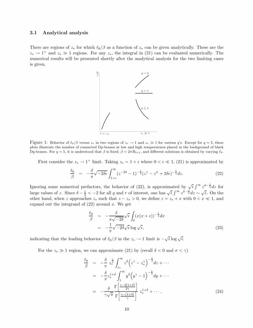
3.1 Analytical analysis

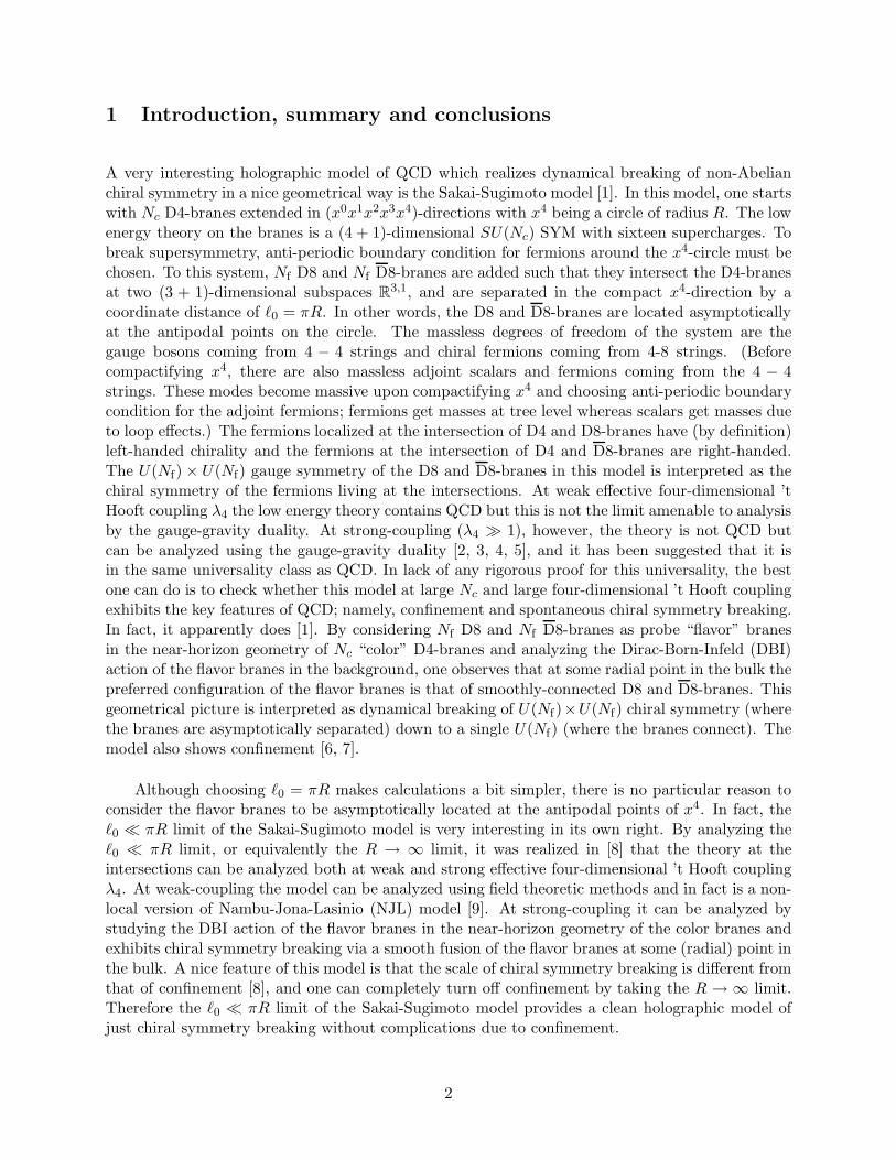
There are regions of z∗ for which ℓ0/β as a function of z∗ can be given analytically. These are thez∗ → 1+ and z∗ ≫ 1 regions. For any z∗, the integral in (21) can be evaluated numerically. Thenumerical results will be presented shortly after the analytical analysis for the two limiting casesis given.

q = 6

q = 5

q ≤ 4

ℓ0β

1← z∗ z∗ ≫ 1

Figure 1: Behavior of ℓ0/β versus z∗ in two regions of z∗ → 1 and z∗ ≫ 1 for various q’s. Except for q = 5, theseplots illustrate the number of connected Dp-branes at low and high temperatures placed in the background of blackDq-branes. For q = 5, it is understood that β is fixed; β = 2πR5+1, and different solutions is obtained by varying ℓ0.

First consider the z∗ → 1+ limit. Taking z∗ = 1 + ǫ where 0 < ǫ ≪ 1, (21) is approximated by

ℓ0

β∼ − δ

π

√−2δǫ

∫ ∞

1+ǫ(z−2δ − 1)−

12 (zγ − zσ + 2δǫ)−

12 dz. (22)

Ignoring some numerical prefactors, the behavior of (22), is approximated by√

ǫ∫ ∞

zδ− γ2 dz for

large values of z. Since δ− γ2 < −2 for all q and r of interest, one has

√ǫ∫ ∞

zδ− γ2 dz ∼ √

ǫ. On theother hand, when z approaches z∗ such that z − z∗ > 0, we define z = z∗ + x with 0 < x ≪ 1, andexpand out the integrand of (22) around x. We get

ℓ0

β∼ − δ

π√−2δ

√ǫ

∫

0(x(x + ǫ))−

12 dx

∼ − 1

π

√−2δ

√ǫ log

√ǫ, (23)

indicating that the leading behavior of ℓ0/β in the z∗ → 1 limit is −√ǫ log

√ǫ.

For the z∗ ≫ 1 region, we can approximate (21) by (recall δ < 0 and σ < γ)

ℓ0

β∼ − δ

πz

γ2∗

∫ ∞

z∗

zδ(

zγ − zγ∗)− 1

2dz + · · ·

= − δ

πz1+δ∗

∫ ∞

1yδ

(

yγ − 1)− 1

2dy + · · ·

= − δ

γ√

π

Γ[

γ−2(1+δ)2γ

]

Γ[

γ−(1+δ)γ

] z1+δ∗ + · · · , (24)

10

where · · · represents terms subleading in z∗, and in the second line in (24) we have changed thevariable from z to y = z/z∗. Thus, aside from a numerical factor, the z∗ → ∞ limit of (21) reads

ℓ0

β∼ z1+δ

∗ . (25)

This expression is identical to the one derived for the zero temperature case in [12]. This resemblanceis not accidental because the large z∗ limit corresponds to having a turning point very far awayfrom the horizon of the background geometry. The results obtained for this limit should then matchthose derived for the zero temperature case. An interesting feature of (25) is that for the blackD5-branes ℓ0/(2πR5+1) is independent of z∗ and approaches a constant value of 1/(r + 3). Thisvalue has been argued in [12] to be around the scale of non-locality of the low energy effectivetheory on D5-branes. The analysis for the dynamics of the flavor branes placed in the thermal D5-brane geometry is the same as the analysis when they are placed in the zero temperature D5-branegeometry. The zero temperature analysis has already been done in [12] where it was found thatthere exist an infinite number of connected solutions for one specific value of ℓ0 = 2πR5+1/(r + 1),and none for other ℓ0’s.

Analyzing (21) for the two regions of z∗ → 1+ and z∗ ≫ 1, the minimum crude conclusion thatone can draw is that for small enough ℓ0/β there exist two connected solutions (one closer to thehorizon which we will name ”long” connected solution, and the other farther away from it named”short” connected solution) for q ≤ 4 and only one curved solution for q = 6. For q = 5 and forT < (2πR5+1)

−1, there exists an infinite number of connected solutions for just ℓ0 = 2πR5+1/(r+1)and none for others. On the other hand, for T = (2πR5+1)

−1, there is only one connected solutiongiven that ℓ0 ≪ 2πR5+1. The analysis for the two z∗ regions has been summarized in Figure 1.

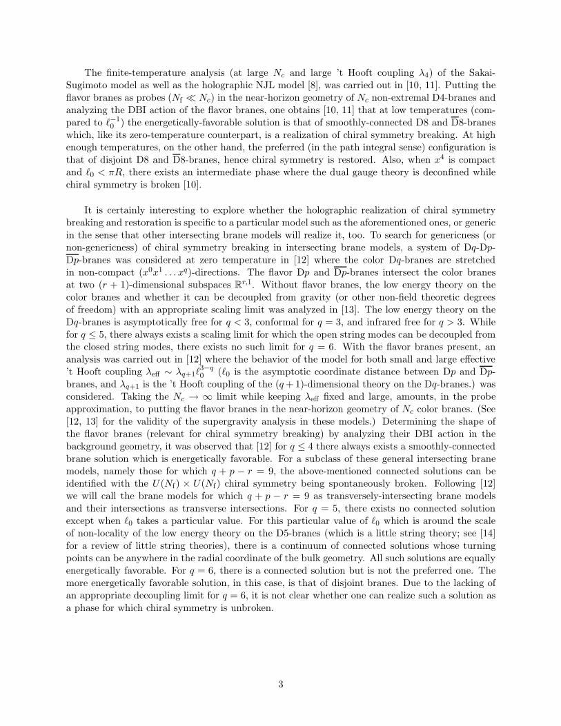
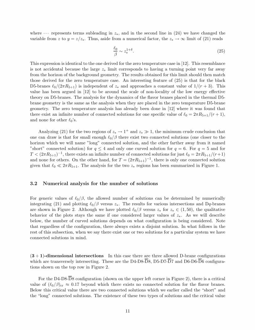
3.2 Numerical analysis for the number of solutions

For generic values of ℓ0/β, the allowed number of solutions can be determined by numericallyintegrating (21) and plotting ℓ0/β versus z∗. The results for various intersections and Dq-branesare shown in Figure 2. Although we have plotted ℓ0/β versus z∗ for z∗ ∈ (1, 50), the qualitativebehavior of the plots stays the same if one considered larger values of z∗. As we will describebelow, the number of curved solutions depends on what configuration is being considered. Notethat regardless of the configuration, there always exists a disjoint solution. In what follows in therest of this subsection, when we say there exist one or two solutions for a particular system we haveconnected solutions in mind.

(3 + 1)-dimensional intersections In this case there are three allowed D-brane configurationswhich are transversely intersecting. These are the D4-D8-D8, D5-D7-D7 and D6-D6-D6 configura-tions shown on the top row in Figure 2.

For the D4-D8-D8 configuration (shown on the upper left corner in Figure 2), there is a criticalvalue of (ℓ0/β)cr ≈ 0.17 beyond which there exists no connected solution for the flavor branes.Below this critical value there are two connected solutions which we earlier called the “short” andthe “long” connected solutions. The existence of these two types of solutions and the critical value

11

of 0.17 were already noted by the authors of [11] in the their analysis of the holographic NJLmodel at finite temperature. We will see in the next section that the short solution is always moreenergetically favorable to the long one. Since there also exists a disjoint solution, determining thechirally-broken or chirally-symmetric phase of the dual field theory (which is a non-local versionof the NJL model [8]) is just a matter of comparing the free energies of the disjoint and shortconnected solution. This will be done in the next section.

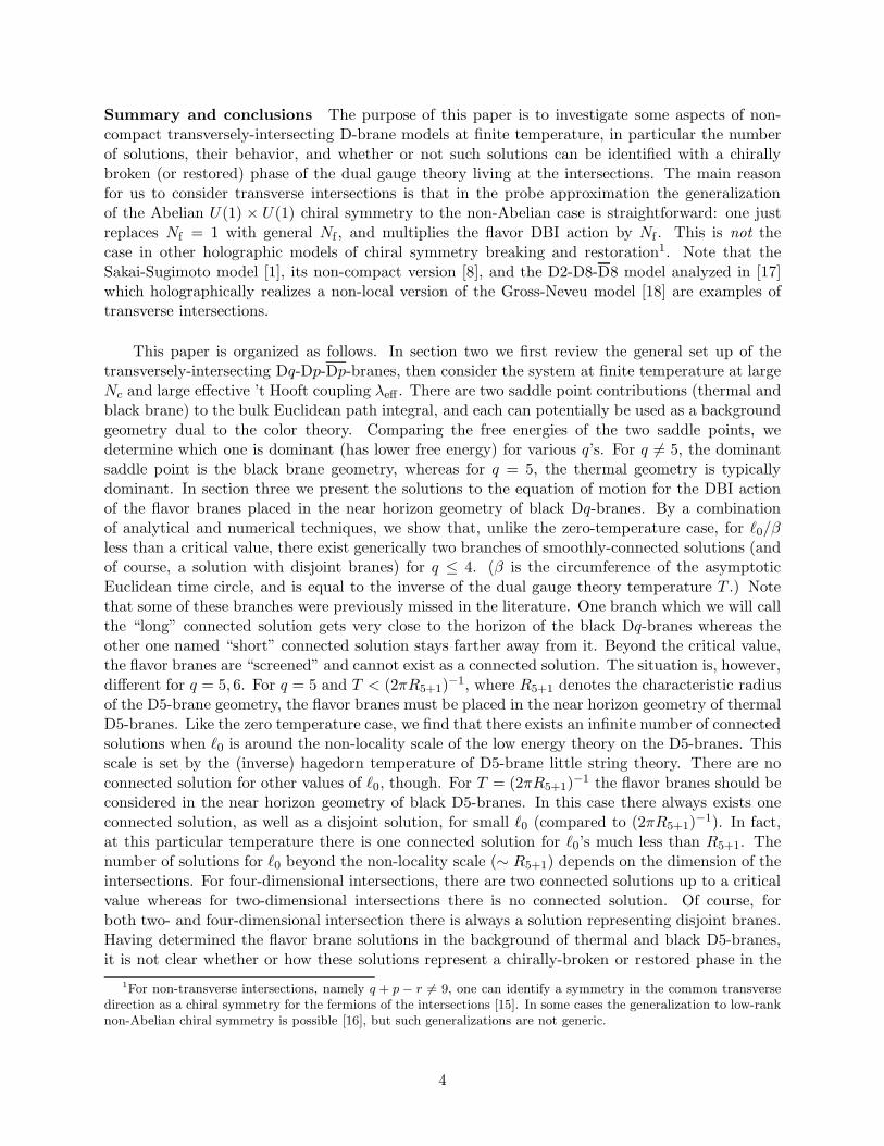
The analysis for the D5-D7-D7 and D6-D6-D6 cases are, however, more subtle, and the holo-graphic interpretation of the solutions is less transparent for reasons to be mentioned below. Forthe D5-D7-D7 configuration at temperature T = (2πR5+1)

−1, there are two critical values of(ℓ0/(2πR5+1))cr ≈ 0.168 and 0.175. For ℓ0/(2πR5+1) < 0.168 there is always one connected solu-tion, for 0.168 < ℓ0/(2πR5+1) < 0.175 there are two, and for ℓ0/(2πR5+1) > 0.175 there exists none.Comparing these results to the ones obtained for the zero-temperature D5-D7-D7 configuration,one observes that while at zero temperature [12], there are either an infinite number of solutionsor none, at T = (2πR5+1)

−1 there are different numbers of solutions (one, two, or none) depend-ing on what values ℓ0 take; see Figures 2 and 3. For D5-D7-D7 configuration at temperaturesT < (2πR5+1)

−1, the situation is the same as the zero temperature case. There exist connectedsolutions only for a specific value of ℓ0 = πR5+1/3. Indeed, there are an infinite number of suchsolutions; see Figure 3.

For D6-D6-D6 configuration, the situation is simpler. For any ℓ0/β there always exists one andonly one connected solution. As we will see in the next section all these connected solutions are lessenergetically favorable compared to disjoint solutions. The observation that for color D6-branesat finite temperature there is always one connected solution, hence no ”screening length”, is inaccord with the fact that the near horizon geometry of D6-branes cannot be decoupled from thegravitational modes of the bulk geometry [13].

(1 + 1)-dimensional intersections In this case, there are five allowed configurations (shown onthe second and third rows in Figure 2), namely D2-D8-D8, D3-D7-D7, D4-D6-D6, D5-D5-D5 andD6-D4-D4. Configurations with q ≤ 4 show similar behavior. For q ≤ 4 there always exists acritical (ℓ0/β)cr beyond which connected solutions cease to exist. The critical value obtained fromFigure 2 is (ℓ0/β)cr ≈ 0.225, 0.223, 0.227 for color D2, D3 and D4-branes, respectively. Below thesecritical values there are two solutions, the short and long solutions2.

For the D5-D5-D5 system at T = (2πR5+1)−1, below a critical value of (ℓ0/(2πR5+1))cr ≈ 0.251

there is always one solution whereas above this value connected solutions do not exist. Notethe difference (depicted in Figure 3) of this case with the D5-D7-D7 system: for the D5-D5-D5configuration, there is no range of ℓ0/(2πR5+1) for which there exist the short and long solutions.Like the D5-D7-D7 configuration, for the D5-D5-D5 system at T < (2πR5+1)

−1, there is an infinitenumber of connected solutions when 2ℓ0 = πR5+1 and none for other ℓ0’s.

For the D6-D4-D4 configuration, there is always one connected solution for arbitrary values ofℓ0/β. Notice that the behavior of the flavor branes in the geometry of color D5 and D6-branes with(1+1)-dimensional intersections is qualitatively the same as their behavior with (3+1)-dimensional

2The authors of [17] studied the D2-D8-D8 system at finite temperature but missed the existence of the longconnected solution.

12

intersections.

5 10 15 20z*

0.1

0.2

0.3

l0Β D5-D5- D5

10 20 30 40 50z*

0.5

1

1.5

2

l0Β D6-D4- D4

5 10 15 20z*

0.1

0.2

0.3

l0Β D2-D8- D8

5 10 15 20z*

0.1

0.2

0.3

l0Β D3-D7- D7

10 20 30 40 50z*

0.1

0.2

0.3

l0Β D4-D6- D6

5 10 15 20z*

0.05

0.1

0.15

0.2

l0Β D4-D8- D8

5 10 15 20z*

0.1

0.15

0.2

l0Β D5-D7- D7

5 10 15 20z*

0.3

0.6

0.9

l0Β D6-D6- D6

Figure 2: Behavior of ℓ0/β versus z∗ obtained numerically for generic values z∗ for various q’s and intersections ofinterest, i.e. r = 1 and r = 3. The blue plots show the behavior for 3+1 intersections whereas the red plots show thebehavior for 1 + 1 intersections. These plots show the number of connected Dp-branes (for all temperatures) placedin the background of black Dq-branes. For q = 5, the temperature T is fixed: T = (2πR5+1)

−1. Except for q = 5, 6,such solutions can potentially be realized as different phases of the holographic dual theories.

4 Energy of the configurations

As we saw in the previous section there are typically more than one solution for a given ℓ0/β.In fact, just to recap, for ℓ0/β less than a critical value there are generically three branches ofsolutions for q ≤ 4; one disjoint and two connected solutions. There are also an infinite number ofsolutions for q = 5 at T < (2πR5+1)

−1 as long as ℓ0 = 2πR5+1/(r + 3). There are two branchesof solutions for q = 6 for any ℓ0/β; one disjoint and one connected solution. Since there arevarious configurations for a particular value of ℓ0/β, one needs to compare their on-shell actions todetermine which configuration is more energetically favorable. In this section we analyze the energyof these configurations by a combination of analytical and numerical techniques. The energy ofthese configurations by themselves is infinite. We regulate the energies of connected configurationsby subtracting from them the energy of disjoint configurations

E = limΛ→∞

∫ Λ

z∗

dz zσ2

(

1 − zγ∗ − zσ

∗zγ − zσ

)− 1

2 −∫ Λ

1dz z

σ2

, (26)

where Λ is a cutoff and the difference in energy E is related to E as

E = −δβ2

πC(q, r) u

γ2

T

∫

drx E. (27)

13

ℓ0β

1← z∗ z∗ →∞

16

D5−D7−D7

ℓ0

y∗ →∞0← y∗

16

D5−D7−D7at finite temperature at zero temperature

D5−D5−D5 D5−D5−D5at zero temperatureat finite temperature

ℓ0β

14

14

ℓ0

1← z∗ 0← y∗ y∗ →∞z∗ →∞

Figure 3: The two plots on the left hand side show the number of connected solutions for the flavor D7 andD5-branes in the background of black D5-branes at T = (2πR5+1)

−1. The plots on the right hand side, on theother hand, show the number of connected solutions for the same flavor branes in the background of thermal (orzero temperature) D5-branes. z∗’s represent the turning points of the connected flavor branes in the black D5-branegeometry while y∗’s are the turning points in the background of thermal D5-branes.

4.1 Analytical analysis

The integral in (26) is complicated and as far as we know cannot be integrated analytically forgeneric values of z∗. However, like the integral in (21), there are two regions of z∗ → 1 and z∗ ≫ 1for which we can integrate E(z∗) analytically. In the z∗ → 1 limit, it can be shown that E ispositive for all q and r. Indeed, let’s rewrite (26) as follows

EΛ =

∫ Λ

z∗

dz zσ2

[(

1 − zγ∗ − zσ

∗zγ − zσ

)− 1

2 − 1]

−∫ z∗

1dz z

σ2

=(

∫ z′∗

z∗

dz zσ2

[(

1 − zγ∗ − zσ

∗zγ − zσ

)− 12 − 1

]

−∫ z∗

1dz z

σ2

)

+

∫ Λ

z′∗

dz zσ2

[(

1 − zγ∗ − zσ

∗zγ − zσ

)− 12 − 1

]

. (28)

The last integral in (28) is positive for any z′∗. If z∗ = 1 + ǫ, we can choose z′∗ = 1 + 3ǫ and thedifference in the bracket is estimated to be

ǫ(√

6 − 2) + ǫ(

log(√

2 +√

3) − 1)

+ o(ǫ2), (29)

which is also positive.

14

1← z∗

E

z∗ ≫ 1

q ≤ 4

q = 6

Figure 4: Behavior of E versus z∗ obtained numerically for generic values of z∗ for various q’s.

Approximating (26) in the z∗ ≫ 1 region yields

EΛ ∼∫ Λ

z∗

dz zδ+γ(

zγ − zγ∗)− 1

2 −∫ Λ

1dz z

σ2 ,

=

∫ Λ

z∗

dz zδ+γ(

zγ − zγ∗)− 1

2 −∫ Λ

0dz z

σ2

+2

σ + 2. (30)

Note that in the large z∗ limit, z∗ ≃ z0 where z0 = u0/uT . As a result, from (30) we see thatthe energy of the connected configurations approaches their zero temperature value obtained in[12]. This is expected since in this regime the connected flavor branes are very far away from thehorizon hence receive little effect from it. The disjoint configuration, on the other hand, alwayskeeps in touch with the horizon and gets a finite temperature contribution − 2

σ+2 . The term inthe curly bracket of (30) is already computed in [12] in terms of Beta functions, giving an energydifference of

E = limΛ→∞EΛ

=1

γz

γ2+δ+1

∗ B[

− 1

2− δ + 1

γ,1

2

]

+2

σ + 2. (31)

Since z∗ ≫ 1, the last term is irrelevant in determining the sign of E. We see immediately thatE > 0 for q ≥ 6 and E < 0 for q ≤ 4. For q = 5, the Beta function vanishes, and a more carefulinvestigation must be made to determine the sign of E. It turns out that in going from (26) to(30), we have over-estimated the energy for the joined brane configurations: there is a correction

with leading behavior ∼ −z(r−1)/2∗ for large z∗. Thus, for q = 5 we have E < 0 for r > 1, while the

analytic analysis is not reliable for r = 1. The analytic results for the two aforementioned limits ofz∗ are summarized in Figure 4.

15

0.1 0.2 0.3 0.4l0Β

-2

-1

1

ã D5-D5- D5

0.1 0.2 0.3l0Β

0.25

0.5

ã D6-D4- D4

0.1 0.2 0.3l0Β

-0.1

-0.05

0.05

0.1

ã D2-D8- D8

0.1 0.2 0.3l0Β

-0.2

-0.1

0.1

0.2

ã D3-D7- D7

0.1 0.2 0.3l0Β

-1

-0.5

0.5

ã D4-D6- D6

0.05 0.1 0.15 0.2l0Β

-0.3

-0.1

0.1

ã D4-D8- D8

0.1 0.2l0Β

-1

-0.5

0.5

1

ã D5-D7- D7

0.1 0.2 0.3LΒ

0.25

0.5

ã D6-D6- D6

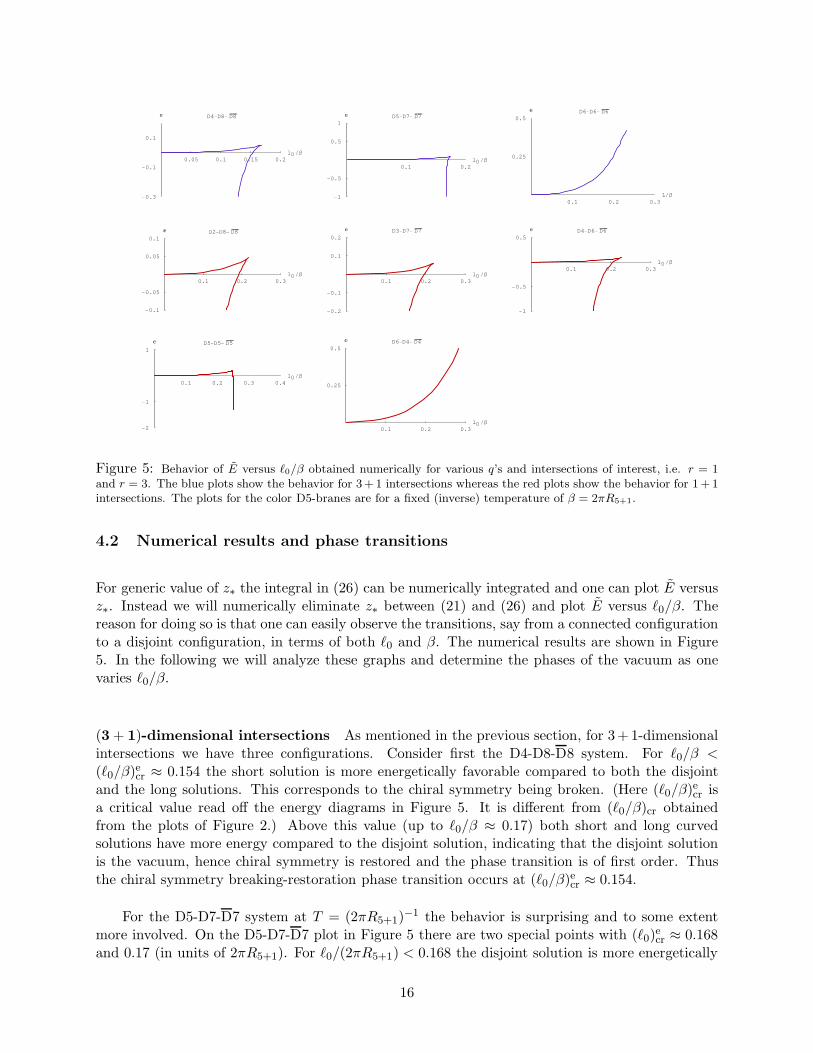
Figure 5: Behavior of E versus ℓ0/β obtained numerically for various q’s and intersections of interest, i.e. r = 1and r = 3. The blue plots show the behavior for 3+ 1 intersections whereas the red plots show the behavior for 1+ 1intersections. The plots for the color D5-branes are for a fixed (inverse) temperature of β = 2πR5+1.

4.2 Numerical results and phase transitions

For generic value of z∗ the integral in (26) can be numerically integrated and one can plot E versusz∗. Instead we will numerically eliminate z∗ between (21) and (26) and plot E versus ℓ0/β. Thereason for doing so is that one can easily observe the transitions, say from a connected configurationto a disjoint configuration, in terms of both ℓ0 and β. The numerical results are shown in Figure5. In the following we will analyze these graphs and determine the phases of the vacuum as onevaries ℓ0/β.

(3 + 1)-dimensional intersections As mentioned in the previous section, for 3+ 1-dimensionalintersections we have three configurations. Consider first the D4-D8-D8 system. For ℓ0/β <(ℓ0/β)ecr ≈ 0.154 the short solution is more energetically favorable compared to both the disjointand the long solutions. This corresponds to the chiral symmetry being broken. (Here (ℓ0/β)ecr isa critical value read off the energy diagrams in Figure 5. It is different from (ℓ0/β)cr obtainedfrom the plots of Figure 2.) Above this value (up to ℓ0/β ≈ 0.17) both short and long curvedsolutions have more energy compared to the disjoint solution, indicating that the disjoint solutionis the vacuum, hence chiral symmetry is restored and the phase transition is of first order. Thusthe chiral symmetry breaking-restoration phase transition occurs at (ℓ0/β)ecr ≈ 0.154.

For the D5-D7-D7 system at T = (2πR5+1)−1 the behavior is surprising and to some extent

more involved. On the D5-D7-D7 plot in Figure 5 there are two special points with (ℓ0)ecr ≈ 0.168

and 0.17 (in units of 2πR5+1). For ℓ0/(2πR5+1) < 0.168 the disjoint solution is more energetically

16

favorable, hence chiral symmetry in the dual theory is intact given that such a solution can representa valid phase of the dual theory. For 0.168 < ℓ0/(2πR5+1) < 0.17 there are three kinds of solutions,disjoint, short and long. It turns out that the short solution has less energy than the other twoindicating that chiral symmetry is broken. For ℓ0/(2πR5+1) > 0.17 the disjoint solution becomesmore energetically favorable, hence potentially chiral symmetry gets restored. For temperaturesless than (2πR5+1)

−1, the situation is the same as the zero temperature case: there are an infinitenumber of connected solutions when 3ℓ0 = πR5+1, each equally energetically favored, and each ofthem more favored over the disjoint solution. The existence of such solutions may be rooted in thefact that the low energy theory on the color D5-branes is a non-local field theory, a little stringtheory. Due to the fact that in the case of background D5-brane geometry the dual field theorydegrees of freedom cannot be totally decoupled from non-field theoretic degrees of freedom, it is notclear to us whether such solutions can represent a chirally-broken phase of the dual gauge theorydespite the fact that, geometrically, they are smoothly connected.

For the D6-D6-D6 system, the disjoint solution is always favorable, although it is not clearwhether one can give a holographic interpretation that the “dual” field theory is in a chirally-symmetric phase. This is because there exists no decoupling limit suitable for holography in thecase of background D6-branes.

(1 + 1)-dimensional intersections For (1+1)-dimensional intersections, there are five allowedconfigurations. Among these the models based on background Dq-branes with q ≤ 4 exhibitsimilar behaviors to their counterparts with (3+1)-dimensional intersection. That is to say forsufficiently low temperatures (compared to 1/ℓ0) chiral symmetry is broken while above a criticaltemperature it gets restored. The critical values at which this (first order) phase transition occursare (ℓ0/β)ecr ≈ 0.191, 0.196 and 0.206 for color D2, D3 and D4-branes, respectively.

The model with color D5-branes again shows some surprises. Because of the mixing be-tween the field theoretic and non-field theoretic degrees of freedom in holography involving back-ground D5-branes, we have no evidence that different behaviors of the flavor branes represent,via holographic point of view, either chirally-symmetric or chirally-broken phases of the dualfield theory. Nevertheless, one finds the following results. At T = (2πR5+1)

−1 and for smallenough ℓ0 (ℓ0 < (ℓ0)

ecr ≈ 0.2498 × 2πR5+1) the disjoint solution is preferred. Increasing ℓ0 up to

ℓ0/(2πR5+1) < 0.251 will result in a phase where the connected solution is favorable. This phaseappears in our plot because we put a cutoff of Λ = 5 to regulate the energy integral. Increasing thecutoff will decrease the range of ℓ0 for which this phase exists. It is plausible that in the Λ → ∞limit this phase disappears although our numerics does not allow us to check this explicitly. Stickingfor now with the cutoff we chose, if one increases ℓ0 further, there will be another phase transitionto a phase where the disjoint solution becomes favored. Due to space limitations, the resolutionof the D5-D5-D5 plot in Figure 5 does not allow one to see all these phases. For temperaturesless than (2πR5+1)

−1, like the zero temperature case, there are an infinite number of connectedsolutions for ℓ0 = πR5+1/2, each equally energetically favored, and none for other ℓ0’s. Each ofthese connected solutions is more favored over the disjoint solution. For the D6-D4-D4 system,there is no phase transition and it is always the disjoint solution which is energetically favorable.

17

5 Transverse intersections at finite temperature with compact xq

An interesting property of the models we are studying here is that when xq is compact the scaleof chiral symmetry breaking is generically different from the scale of confinement which results inadditional phases. For example, for the Sakai-Sugimoto model at finite temperature, it was shown[10] that there exists an intermediate phase where the system is deconfined while chiral symmetryis broken.

At finite temperature and xq direction being compact (with a radius of Rc), there are threegeometries where the topology of the t − xq submanifold is S1 × S1. One is a geometry which hasthe metric

ds2 =

(

u

Rq+1

)7−q2 (

dt2 + d~x2 + g(u)(dxq)2)

+

(

u

Rq+1

)− 7−q2 ( du2

g(u)+ u2dΩ8−q

2)

, (32)

with

g(u) = 1 −(uKK

u

)7−q. (33)

We will call this geometry the thermal geometry. Although the Euclidean time period β is arbitraryin this geometry, the xq-circle cannot have arbitrary periodicity. In order for this geometry to besmooth at u = uKK in the xq − u submanifold, one has to have

∆xq = βc =4π

7 − q

(

Rq+1

uKK

)7−q2

uKK, (34)

where we have defined βc = 2πRc. Although we do not specify the q-dependence of βc and Rc,one should keep in mind that they depend on uKK and Rq+1 differently through (34) depending onwhat value for q is given. There is another geometry whose metric takes the form

ds2 =

(

u

Rq+1

)7−q2 (

dt2 + d~x2 + (dxq)2)

+

(

u

Rq+1

)− 7−q2 (

du2 + u2dΩ8−q2)

. (35)

There is also the black brane geometry which is basically the same as (2) but with xq compact,and has the (Euclidean) metric

ds2 =

(

u

Rq+1

)7−q2

(

f(u)dt2 + d~x2 + (dxq)2)

+

(

u

Rq+1

)− 7−q2

( du2

f(u)+ u2dΩ8−q

2)

, (36)

where

f(u) = 1 −(uT

u

)7−q. (37)

In this geometry the xq-circle has arbitrary periodicity whereas β is fixed by

β =4π

7 − q

(Rq+1

uT

)7−q2

uT . (38)

For all three geometries, the dilaton φ, and the q-form RR-flux Fq are given in (6); see the appendixfor more details. Also, Rq+1 is given in (4).

18

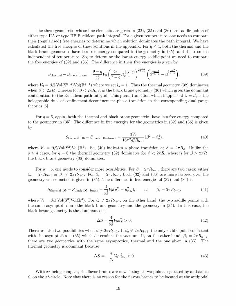
The three geometries whose line elements are given in (32), (35) and (36) are saddle points ofeither type IIA or type IIB Euclidean path integral. For a given temperature, one needs to comparetheir (regularized) free energies to determine which solution dominates the path integral. We havecalculated the free energies of these solutions in the appendix. For q ≤ 4, both the thermal and theblack brane geometries have less free energy compared to the geometry in (35), and this result isindependent of temperature. So, to determine the lowest energy saddle point we need to comparethe free energies of (32) and (36). The difference in their free energies is given by

Sthermal − Sblack brane =9 − q

g2s

V9

(

4π

7 − qR

12(7−q)

q+1

)2 7−q5−q

(

β2 q−7

5−q − β2 q−7

5−qc

)

, (39)

where V9 = ββcVol(S8−q)Vol(Rq−1) where we set ls = 1. Thus the thermal geometry (32) dominateswhen β > 2πRc whereas for β < 2πRc it is the black brane geometry (36) which gives the dominantcontribution to the Euclidean path integral. This phase transition which happens at β = βc is theholographic dual of confinement-deconfinement phase transition in the corresponding dual gaugetheories [6].

For q = 6, again, both the thermal and black brane geometries have less free energy comparedto the geometry in (35). The difference in free energies for the geometries in (32) and (36) is givenby

Sthermal D6 − Sblack D6−brane =3V9

16π2g2sR6+1

(β2 − β2c ), (40)

where V9 = ββcVol(S2)Vol(R5). So, (40) indicates a phase transition at β = 2πRc. Unlike theq ≤ 4 cases, for q = 6 the thermal geometry (32) dominates for β < 2πRc whereas for β > 2πRc

the black brane geometry (36) dominates.

For q = 5, one needs to consider more possiblities. For β = 2πR5+1, there are two cases: eitherβc = 2πR5+1 or βc 6= 2πR5+1. For βc = 2πR5+1, both (32) and (36) are more favored over thegeometry whose metric is given in (35). The difference in free energies of (32) and (36) is

Sthermal D5 − Sblack D5−brane =4

g2s

V9(u2T − u2

KK), at βc = 2πR5+1. (41)

where V9 = ββcVol(S3)Vol(R4). For βc 6= 2πR5+1, on the other hand, the two saddle points withthe same asymptotics are the black brane geometry and the geometry in (35). In this case, theblack brane geometry is the dominant one

∆S =4

g2s

V9u2T > 0. (42)

There are also two possibilities when β 6= 2πR5+1. If βc 6= 2πR5+1, the only saddle point consistentwith the asymptotics is (35) which determines the vacuum. If, on the other hand, βc = 2πR5+1,there are two geometries with the same asymptotics, thermal and the one given in (35). Thethermal geometry is dominant because

∆S = − 4

g2s

V9u2KK < 0. (43)

With xq being compact, the flavor branes are now sitting at two points separated by a distanceℓ0 on the xq-circle. Note that there is no reason for the flavors branes to be located at the antipodal

19

points on the circle. As before, we consider the transverse intersections of the flavor and the colorbranes, and choose the same embeddings and boundary conditions for the flavor branes as we didin (10) and (11) except that now ℓ0 ≤ πRc. In what follows, we will focus on q ≤ 4 cases andconsider both low and high temperature phases of the background. In particular, we would liketo know whether there always exists a range of temperature above the deconfinement temperaturewhere chiral symmetry is broken.

5.1 Behavior at high and low temperatures

For temperatures above the deconfinement temperature βc the profile of the flavor branes takesessentially the same form as it did when xq was non-compact, hence, indicating the existence ofshort and long (smoothly) connected solutions. Note that when xq is compact, for a fixed ℓ0, thereis now a lower bound on ℓ0/β set by the deconfinement temperature. For completeness, we haveplotted ℓ0/β versus z∗ (z∗ being the radial position at which the brane and anti-brane smoothlyjoin) in Figure 6. The lower dotted line in each plot represents the deconfinement temperature.As an example, we chose it to be at βc = 10ℓ0. The upper dotted line shows chiral symmetrybreaking-restoration phase transition which comes from comparing the energies of connected anddisjoint solutions. One can show, using energy considerations, that below the upper dotted linechiral symmetry is broken in a deconfined phase via short connected solution while it is restoredabove the line (where we have deconfinement with chiral symmetry restoration).

1 3 5

z*

0.05

0.1

0.15

0.2

l0 Β

D4-D8-D8

1 2 3

z*

0.1

0.2

0.3

l0 Β

D2-D8-D8

1 2 3 4

z*

0.1

0.2

0.3

l0 Β

D3-D7-D7

1 4 7 10

z*

0.1

0.2

0.3

l0 Β

D4-D6-D6

Figure 6: Behavior of ℓ0/β versus z∗ above the deconfinement temperature for q = 2, 3, 4. The lower dotted linerepresents a transition to the confined phase whereas the upper dotted line represents chiral symmetry breaking-restoration phase transition.

20

In the low temperature regime where the system is in a confined phase, the DBI action for theflavor branes in the thermal background (32) now reads (with gauge fields set equal to zero)

SDBI = β C(q, r)

∫

drx dxq uγ2

[

g(u) +1

g(u)

( u

Rq+1

)2δu

′2]

12, (44)

where C(q, r), γ and δ have all been defined in (14). The equation of motion for the profile is now

uγ2 g(u)

[

g(u) +1

g(u)

( u

Rq+1

)2δu

′2]− 1

2= w

γ2

0 , (45)

with w0 parameterizing the solutions. There exists a solution with w0 = 0 representing disjoint Dpand Dp-branes descending down to u = uKK. For w0 6= 0, solving (45) for u

′yields

u′2

=1

w0γ

( u

Rq+1

)−2δg(u)2

(

uγg(u) − w0γ)

. (46)

Denoting the possible turning point(s) by w∗, analysis of (46) shows that u ≥ w∗ > uKK, with w∗satisfying

wγ∗ − wσ

∗u−2δKK − wγ

0 = 0, (47)

where σ has been defined as before. Integrating (46) gives

xq(y) = − δ

2πβc(y

γ∗ − yσ

∗ )12

∫ y

y∗

(

y−2δ − 1)−1(

yγ − yσ − (yγ∗ − yσ

∗ ))− 1

2dy, (48)

where we have defined y = (u/uKK) ∈ (1,∞), and y∗ = w∗/uKK. Using (48) we can relate y∗ to ℓ0

ℓ0

βc= − δ

π(yγ

∗ − yσ∗ )

12

∫ ∞

y∗

(

y−2δ − 1)−1(

yγ − yσ − (yγ∗ − yσ

∗ ))− 1

2dy. (49)

The analysis of ℓ0/βc as a function of y∗ determines the number of solutions. ℓ0/βc versus y∗ hasbeen numerically plotted in Figure 7 for intersections of interest and for q = 2, 3, 4. As it is seenfrom Figure 7, there is always one smoothly connected solution (as well as a disjoint solution).The red and blue plots represent smoothly connected solutions for (1+1)-dimensional and (3+1)-dimensional intersections, respectively.

For the energy of the connected solutions, one obtains

E = −δβ

πβcC(q, r) u

γ2

KK

∫

dxr E, (50)

where

E = limΛ→∞

∫ Λ

y∗

dy yσ2

(

1 − y2δ)− 1

2(

1 − yγ∗ − yσ

∗yγ − yσ

)− 1

2 −∫ Λ

1dy

(

1 − y2δ)− 1

2y

σ2

, (51)

and Λ is a cutoff. Like the previous sections, one can numerically eliminate y∗ between (49) and (51)and plot E versus ℓ0/βc. Although we have not shown the plots here, one can check (numerically)that the smoothly connected solutions are always more energetically favorable compared to thedisjoint solutions.

21

1 5 9

w*

0.2

0.4

0.6

l0 Βc

D4-D8-D8

1 2 3

w*

0.2

0.4

0.6

l0 Βc

D2-D8-D8

1 3 5

w*

0.2

0.4

0.6

l0 Βc

D3-D7-D7

1 5 9

w*

0.2

0.4

0.6

l0 Βc

D4-D6-D6

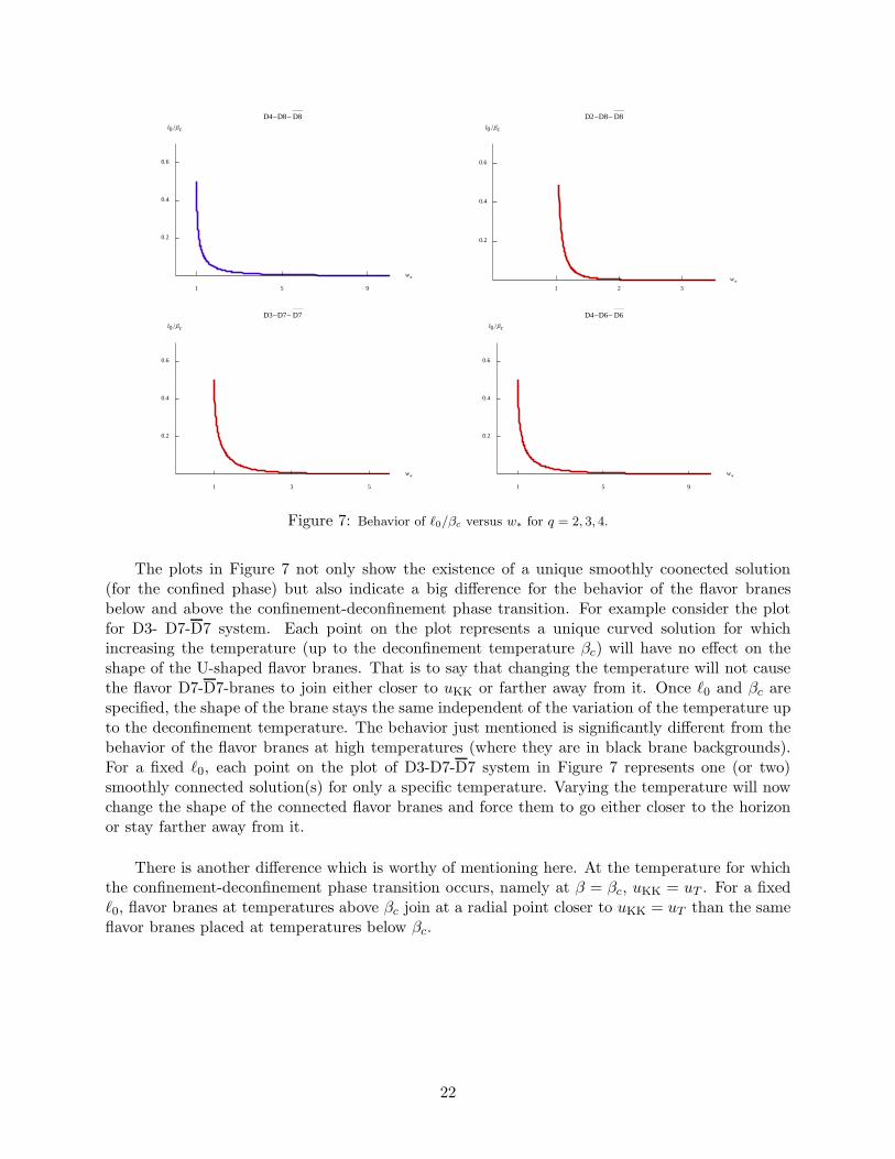
Figure 7: Behavior of ℓ0/βc versus w∗ for q = 2, 3, 4.

The plots in Figure 7 not only show the existence of a unique smoothly coonected solution(for the confined phase) but also indicate a big difference for the behavior of the flavor branesbelow and above the confinement-deconfinement phase transition. For example consider the plotfor D3- D7-D7 system. Each point on the plot represents a unique curved solution for whichincreasing the temperature (up to the deconfinement temperature βc) will have no effect on theshape of the U-shaped flavor branes. That is to say that changing the temperature will not causethe flavor D7-D7-branes to join either closer to uKK or farther away from it. Once ℓ0 and βc arespecified, the shape of the brane stays the same independent of the variation of the temperature upto the deconfinement temperature. The behavior just mentioned is significantly different from thebehavior of the flavor branes at high temperatures (where they are in black brane backgrounds).For a fixed ℓ0, each point on the plot of D3-D7-D7 system in Figure 7 represents one (or two)smoothly connected solution(s) for only a specific temperature. Varying the temperature will nowchange the shape of the connected flavor branes and force them to go either closer to the horizonor stay farther away from it.

There is another difference which is worthy of mentioning here. At the temperature for whichthe confinement-deconfinement phase transition occurs, namely at β = βc, uKK = uT . For a fixedℓ0, flavor branes at temperatures above βc join at a radial point closer to uKK = uT than the sameflavor branes placed at temperatures below βc.

22

6 Discussion

In this paper, we analyzed some aspects of transversely-intersecting Dq-Dp-Dp-branes at finitetemperature. In particular, we mapped out different vacuum configurations which can holographi-cally be identified with chiral symmetry breaking (or restoration) phase of their holographic dualtheories. Although we showed that generically the long connected solutions are less energeticallyfavorable compared to the short connected solutions we did not discuss their stability against smallperturbations. Presumably a stability analysis along the lines of [19] can be done to show that thelong connected solution is unstable against small perturbations. The analysis presented here can begeneralized in various directions. For example, one can add a chemical potential to the setup andlook for new phases as was done in some specific models in [20, 21, 22, 23], or consider the sysytemat background electric and magnetic fields [24, 25, 26] and study the conductivity of the system orthe effect of the magnetic field on the chiral symmetry-restoration temperature. We hope to comeback to these interesting issues in future.

Also, our analysis was entirely based on the DBI action for the flavor Dp-Dp-branes. Intransversely-intersecting D-branes, working with just the DBI (plus the Chern-Simons part ofthe) action misses, from holographic perspectives, an important part of the physics, namely thevev of the fermion bilinear as an order parameter for chiral symmetry breaking. To determine thefermion bilinear from the holographic point of view there should be a mode propagating in thebulk geometry such that asymptotically its normalizable mode can be identified with the vev of thefermion bilinear. The DBI plus the Chern-Simons action cannot give rise to the mass of the localizedchiral fermions either. Note that for transverse intersections one cannot write an explicit mass termfor the fermions of the intersections because there is no transverse space common to both the colorand the flavor branes. So it is not possible to stretch an open string between the color and flavorbranes in the transverse directions. Therefore, the fermion mass must be generated dynamically.It has been argued in [8] that including the dynamics of an open string stretched between theflavor branes into the analysis will address the question of how one can compute fermion mass andbilinear vev in these holographic models. More concretely, the scalar mode of this open string whichtransforms as bifundamental of U(Nf) × U(Nf) has the right quantum numbers to be potentiallyholographically dual to the fermion mass and condensation.

Recently, the authors of [28, 29, 30] shed light on this issue by starting with the so-calledtachyon-DBI action [27] claimed to correctly incorporate the role of the open string scalar mode,the tachyon, in a system of separated Dp-Dp-branes. In fact, it was shown in [29, 30] that forthe Sakai-Sugimoto model at zero temperature, the open string tachyon will asymptotically have anormalizable as well as a non-normalizable mode. They identified the normalizable mode with thevev of the fermion bilinear (order parameter for chiral symmetry breaking) and the non-normalizablemode with the fermion mass. It is not hard to generalize the calculations of [29, 30] to include alltransversely-intersecting Dq-Dp-Dp systems at zero temperature where one finds that there alwaysexist both normalizable and non-normalizable modes for the asymptotic behavior of the tachyon,and in the bulk of the geometry the tachyon condenses roughly at the same radial point wherethe flavor branes smoothly join [31]. The calculation of the fermion mass and condensate fortransversely-intersecting Dq-Dp-Dp systems at finite temperature requires not only considering thetachyon-DBI action of [27] in the black brane background of (2) but also calculating the tachyonpotential as a function of the temperature. In the case of a coincident brane and anti-brane in flatbackground, a partial result for such a calculation was given in [32] (see also [33]). Some attempts in

23

generalizing the results of [32, 33] for separated brane-anti-branes (at least in the case of separatedD8-D8 in flat space) has recently started in [34]. For our purpose of extracting information aboutfermion mass and condensate, knowing the dependence of the tachyon potential for separated flavorDp-Dp-branes seems crucial. Ignoring the temperature dependence on tachyon potential at zerothorder yields unsatisfactory results: It gives rise to the same results as one would have obtainedin the zero temperature case [31]. We know that this is not the right behavior because at zerotemperature there is no chiral phase transition.

Note added in version two There are now two more interesting (and closely related) proposalson how to compute the fermion mass and condensates in transversely-intersecting D-branes. Oneproposal is based on an open wilson line operator whose vev gives the condensate [35] (see also[36, 37] for generalizations) and the other [38] is based on a D6-brane, in the case of the Sakai-Sugimoto model, ending on the flavor D8-D8-branes It would be interesting to understand therelations between these two proposals and the one based on the open string tachyon.

Acknowledgments

We would like to thank P. Argyres, S. Baharian, O. Bergman, and especially J. F. Vazquez-Poritzfor helpful discussions and comments . This work is supported by DOE grant DE-FG02-91ER40709.

A Free energies of possible bulk backgrounds

Following [10] we use the notation adopted in [39] to compute the free energy of possible finitetemperature Dq-brane backgrounds for both compact and non-compact xq-direction. We firstconsider the case of compact xq and as a warm-up first do the computation for D6-branes, thengeneralize it to Dq-branes.

A.1 Compact xq

D6-branes Consider the bosonic part of type IIA supergravity action (in Euclidean signatureand) in string frame

S = −(SEH + Sφ + SRR + SNS),

= −∫

e−2φ√g(R + 4∂φ∂φ) +1

2

∑

q

∫

F(q+2) ∧ ∗F(q+2) +1

2

∫

e−2φH(3). ∧ ∗H(3). (52)

24

Having the near horizon geometry of D6-branes in mind, we choose the following (radial) ansatzfor the metric and RR 7-form C(7)

l−2s ds2 =dτ2 + e2λ(τ)dx2

‖ + e2λ(τ)dx2c + e2ν(τ)dΩ2

2, (53)

C(7) =A dx1 ∧ ... ∧ dx5 ∧ dx6−c ∧ dxc, (54)

where dΩ22 is the line element of the unit two-sphere. Certainly the backgrounds we considered in

this paper can all be put into the form of our ansatz (53). Here τ is the radial coordinate, x‖ are 6(out of 7) worldvolume directions, xc plays the role of time in black D6-brane geometry and x6 inthermal geometry. From now on we set ls = 1. It could be restored into our results by dimensionalanalysis.

The equation of motion of C(7) has the solution

Ae−6λ−λ+2ν = const, (55)

where the dot represents the derivative with respect to τ . Substituting (55) into (52), the RR partof the action reads

− SRR =

∫

Q2e6λ+λ−2νdτ, (56)

where Q2 is an integration constant. It is more convenient to define a new radial coordinatedρ = −eϕdτ , where

ϕ = 2φ − 6λ − λ − 2ν, (57)

in terms of which (56) reads

− SRR = −∫

Q2e6λ+λ−2ν−ϕdρ. (58)

Note that√

ge−2φdτ = −e−2ϕdρ by which the dilaton action is easily computed to give

− Sφ =

∫

4φ′2dρ, (59)

where prime denotes the derivative with respect to ρ . With our metric ansatz (53), the Ricci scalaris

R = 2e−2ν − 42λ2 − 2 ˙λ2 − 6ν2 − 12λ ˙λ − 24λν − 4 ˙λν − 12λ − 2¨λ − 4ν. (60)

Thus, expressed in terms of the ρ coordinate, the Einstein-Hilbert action becomes

− SEH =

∫

Re−2ϕdρ,

=

∫

[

2e−2ν−2ϕ − 42λ′2 − 2λ′2 − 6ν ′2 − 12λ′λ′ − 24λ′ν ′ − 4λ′ν ′ − 12(λ′′ + λ′ϕ′)

−2(λ′′ + λ′ϕ′) − 4(ν ′′ + ν ′ϕ′)]

dρ. (61)

Note that the terms with double primes are total derivatives and are cancelled by adding theGibbons-Hawking term to (61). Using (57), SEH and Sφ add up to give the following simpleexpression

− SEH − Sφ =

∫

(

2e−2ν−2ϕ − 6λ′2 − λ′2 − 2ν ′2 + ϕ′2)

dρ. (62)

25

Putting everything together, the total action reads

S =

∫

(

2e−2ν−2ϕ − 6λ′2 − λ′2 − 2ν ′2 + ϕ′2 − Q2e6λ+λ−2ν)

dρ. (63)

The equations of motion are

λ′′ =Q2

2e−2φ+12λ+2λ, (64)

λ′′ =Q2

2e−2φ+12λ+2λ, (65)

ν ′′ =e−4φ+12λ+2λ+2ν − Q2

2e−2φ+12λ+2λ, (66)

φ′′ =3Q2

2e−2φ+12λ+2λ, (67)

where ϕ has been replaced by φ using (57). Defining Φ = −2φ + 12λ + 2λ, (64), (65) and (67) give

Φ′′ = 4Q2eΦ, (68)

with the following solution

Φ = −2 ln(

√2Q

CC1sinhC1ρ

)

− 2 ln C. (69)

The last term in (69) is there just for convenience. Going back to (64), (65) and (67) and solvingfor λ, λ and φ, one obtains

λ = − 1

4ln

(

√2Q

gsC1sinhC1ρ

)

+ Cλ2 ρ, (70)

λ = − 1

4ln

(

√2Q

gsC1sinhC1ρ

)

+ C λ2 ρ, (71)

φ = − 3

4ln

(

√2Q

gsC1sinhC1ρ

)

+ Cφ2 ρ + ln gs, (72)

with 6Cλ2 + C λ

2 − Cφ2 = 0. The constants C1, Cλ

2 , C λ2 and Cφ

2 are to be determined. DefiningΦ0 = Φ + 2 ln gs, the equation of motion for ν becomes

ν ′′ = eΦ04−2Cφ

2 ρ−4 ln gs+2ν − 1

2Q2eΦ. (73)

If we take 2ν = 34Φ0

+ 2Cφ2 ρ + Cν , the above equation is satisfied if

Cν = ln 2Q2g2s .

Thus, we obtain

ν = −3

4ln

(

√2Q

gsC1sinhC1ρ

)

+ Cφ2 ρ + ln

√2Qgs. (74)

26

In what follows we show that the near horizon geometry of non-extremal D6-branes satisfies(70), (71), (72). This geometry takes the form

ds2 =f−1/2(

dx2‖ + hdx2

c

)

+ f1/2( 1

hdu2 + u2dΩ2

2,)

(75)

e−2φ =g−2s f3/2, (76)

with

f =gsNc

2lsu, and h = 1 − uc

u, (77)

where uc is either uT or uKK (or zero for the geometry given in (35)). The u coordinate is not thesame as ρ. Their relation can be inferred from (70) and (71), and is given by

e2(λ−λ) = e2ρ(Cλ2 −Cλ

2 ) = h, (78)

yielding

ρ =1

2∆C2ln h,

dρ =uc

2u2∆C2

1

hdu, (79)

where ∆C2 = C λ2 − Cλ

2 . Computing e2λ from (70), we have

e2λ =e2Cλ

2 ρ

√

(√2Q

gsC1

)

sinh C1ρ

,

=

√√2C1gs

Q

hCλ

2∆C2

√

hC1

2∆C2 − h−C12∆C2

,

=

√√2C1gs

Q

hCλ

2∆C2

− C14∆C2

√

1 − h−C1∆C2

. (80)

To match e2λ in (80) with f1/2, one has to impose −C1 = ∆C2 and C1 = 4Cλ2 , or

C1 = 4Cλ2 ; C λ

2 = −3C2λ. (81)

Thus, we have

e2λ =√√

2C1gs

Quuc

≡(

2lsugsN

)1/2⇒ Cλ

2 = Qucls2√

2g2sN

. (82)

Taking Cφ2 = 3Cλ

2 , we can match the dilaton with the dilaton of the D6-brane solution (76)

e2φ = e6λ+2 ln gs = g2s

( 2lsu

gsNc

)3/2. (83)

27

Furthermore, from (74), we have

e2ν = 2Q2g2se

6λ = 2Q2g2s

( 2lsu

gsNc

)3/2≡

(gsN

2lsu

)1/2u2 ⇒ N = 2

√2Qls (84)

The final check is the guu component of the metric. To do that, we first need to compute e−2ϕ

which turns out to be

e−2ϕ = e−4φ+12λ+2λ+6ν ,

= e14λ−8Cλ2 ρ+4 ln (

√2Qgs)−4 ln gs ,

=(2lsu

gsN

)7/2h(√

2Q)4. (85)

Hence,

dτ2 = e−2ϕdρ2,

=(2lsu

gsN

)7/2h(√

2Q)4u2

c

4u4(

16(Cλ2 )2

)

1

h2,

=(gsNc

2lsu

)1/2 1

h, (86)

where we have used (82) and (84) to simplify the expression. Thus, the near horizon geometry ofNc D6-branes is indeed a solution to type IIA supergravity equations of motion.

It is now straightforward to plug (70), (71), (72) and (74) into (63) to obtain the on-shell action(free energy). Changing the coordinate from ρ coordinate to u and being careful about the factthat dρ/du is negative, we obtain

S = −V9

∫ ∞

uc

(

− 6λ′2 − λ′2 − 2ν ′2 + ϕ′2)du

dρ+

(

2e−2ν−2ϕ − Q2e6λ+λ−2ν)dρ

du

du (87)

=3

g2s

V9

∫ Λ

uc

du =3

g2s

V9(Λ − uc). (88)

where in the first line prime denotes the u-derivative, and V9 is the volume (in units of string lengthwhich we set equal to one) of space transverse to u: V9 = βVol(S1

xq)Vol(S2)Vol(R5). The free energyis infinite. That is why we put a cutoff u = Λ in the second line to regulate the free energy. Thecutoff drops out when it comes to comparing the free energies of different solutions.

It is clear from (87) that a D6-brane solution of the type (35) has always more free energythan a black D6-brane (36) or a thermal D6-brane (32). Comparing the free energies of the blackand thermal D6-brane geometries, we obtain

Sthermal D6 − Sblack D6−brane =3

g2s

V9(uT − uKK), (89)

=3V9

16π2g2sR6+1

(β2 − β2c ), (90)

where in the second line we have used (34) and (38), and

βc = 2πRc =4π

3

√

R6+1uKK. (91)

Thus, there is a phase transition at β = 2πRc, where the thermal D6-brane geometry dominatesfor β < 2πRc whereas for β > 2πRc the black brane geometry dominates.

28

Dq-branes: general analysis Having gone through the analysis for the D6-brane, calculatingthe free energy of non-extremal Dq-branes is straightforward. The relevant parts of the supergravityaction (in string frame) are

S = −(SEH + Sφ + SRR + SNS),

= −∫

e−2φ√g(R + 4∂φ∂φ) +1

2

∑

q

∫

F(q+2) ∧ ∗F(q+2) +1

2

∫

e−2φH(3) ∧ ∗H(3). (92)

We are interested in backgrounds with H(3) not turned on, and choose the following ansatz for themetric and the RR q-form Cq+1

ds2 = dτ2 + e2λ(τ)dx2‖ + e2λ(τ)dx2

c + e2ν(τ)dΩ2k, (93)

C(q+1) = A dx1 ∧ ... ∧ dxq−1 ∧ dxq−c ∧ dxc, (94)

where k = 8 − q, and dΩ2k is the line element of unit k-sphere. Again, we have set ls = 1. The

equation of motion for C(q+1) has the solution

Ae−qλ−λ+kν = const. (95)

The RR action then becomes

− SRR =

∫

Q2eqλ+λ−kνdτ, (96)

where, again, we denoted the integration constant by Q2. For convenience, we change the variablefrom τ to ρ defined by dρ = −eϕdτ , where

ϕ = 2φ − qλ − λ − kν. (97)

Then

− SRR = −∫

Q2eqλ+λ−kν−ϕdρ. (98)

Following the same argument as we did for q = 6, it is not hard to see that the action (92)takes the form

S =

∫

(

k(k − 1)e−2ν−2ϕ − qλ′2 − λ′2 − kν ′2 + ϕ′2 − Q2eqλ+λ−kν)

dρ. (99)

Having put the action in the above form, the equations of motion are now in order

λ′′ =Q2

2e−2φ+2qλ+2λ (100)

λ′′ =Q2

2e−2φ+2qλ+2λ (101)

ν ′′ = (k − 1)e−2ν−2ϕ − Q2

2e−2φ+2qλ+2λ (102)

φ′′ =(5 − k)Q2

2e−2φ+2qλ+2λ, (103)

29

Define Φ = −2φ + 2qλ + 2λ, (100), then (101) and (103) result in

Φ′′ = 4Q2eΦ, (104)

which yields the following solution

Φ = −2 ln (

√2Q

CC1sinhC1ρ) − 2 ln C. (105)

The last term is there just for convenience. Solving for λ, λ and φ in (100), (101) and (103), weobtain

λ = −1

4ln

(

√2Q

gsC1sinhC1ρ

)

+ Cλ2 ρ, (106)

λ = −1

4ln

(

√2Q

gsC1sinhC1ρ

)

+ C λ2 ρ, (107)

φ = −5 − k

4ln

(

√2Q

gsC1sinh C1ρ

)

+ Cφ2 ρ + ln gs, (108)

with qCλ2 + C λ

2 − Cφ2 = 0. The constants C1, Cλ

2 , C λ2 and Cφ

2 are to be determined. DefineΦ0 = Φ + 2 ln gs, then the equation of motion for ν becomes

ν ′′ = (k − 1)e7−q4

Φ0−2Cφ2 ρ−4 ln gs+2(k−1)ν − 1

2Q2eΦ. (109)

If we take 2(k − 1)ν = q−34 Φ0 + 2Cφ

2 ρ + Cν , then the above equation is satisfied if

Cν = ln2Q2g2

s

(k − 1)2. (110)

Thus, we obtain

ν = − 5 − k

4(k − 1)ln

(

√2Q

gsC1sinh C1ρ

)

+Cφ

2 ρ

k − 1+

1

k − 1ln

√2Qgs

k − 1. (111)

We now check whether the near horizon geometry of non-extremal Dq-branes satisfies (106),(107), (108) and (111). This geometry takes the form

ds2 = f−1/2q

(

dx2‖ + hdx2

c

)

+ f1/2q

(1

hdu2 + u2dΩ2

k

)

, (112)

e−2φ = g−2s f (q−3)/2

q , (113)

where fq =d′qgsNc

(lsu)7−q , d′p = (2√

π)5−qΓ(7−q2 ) and h = 1 − (uc/u)7−q.The relation between u and pho

can is inferred from (106) and (107)

e2(λ−λ) = e2ρ(Cλ2 −Cλ

2 ) = h, (114)

which gives

ρ = 12∆C2

ln h ⇒ dρ = (7−q)u7−qc uq−8

2∆C2

1hdu, (115)

30

where ∆C2 = C λ2 − Cλ

2 . Calculating e2λ from (106), we have

e2λ =e2Cλ

2 ρ

√

(√2Q

gsC1

)

sinhC1ρ

=

√√2C1gs

Q

hCλ

2∆C2

√

hC1

2∆C2 − h−C12∆C2

=

√√2C1gs

Q

hCλ

2∆C2

− C14∆C2

√

1 − h−C1∆C2

. (116)

The only way to make e2λ in (116) to be equal to f1/2q is by imposing −C1 = ∆C2 and C1 = 4Cλ

2 ,or

C1 = 4Cλ2 ; C λ

2 = −3C2λ. (117)

Thus, we have

e2λ =

√√2C1gs

Q

( u

uc

)7−q2 ≡ f−1/2

q ⇒ Cλ2 =

Q(ucls)7−q

4√

2g2sNcd′q

. (118)

Also, the dilaton can be matched to (113) as long as we take Cφ2 = (5 − k)Cλ

2 resulting in

e2φ = e2λ(5−k)+2 ln gs = g2sf

− q−3

2q . (119)

Furthermore, from (111), we have

e2ν =(

√2Qgs

k − 1

)2

k−1e2λ 5−k

k−1 ≡ f1/2q u2 ⇒ Nc =

√2Qlk−1

s

(k−1)d′q. (120)

The final check is the guu component. To do that, we first need to compute e−2ϕ which gives

e−2ϕ = e−4φ+2qλ+2λ+2kν

= e6k+2

k−1λ−8Cλ

2 ρ+ 2kk−1

ln (√

2Qgsk−1

)−4 ln gs . (121)

Hence

dτ2 = e−2ϕdρ2

=(7 − q)2u

2(7−q)c u2(q−8)

64(Cλ2 )2

1

h2e

6k+2

k−1λ−8Cλ

2 ρ+ 2kk−1

ln (√

2Qgsk−1

)−4 ln gsdu2

= f1/2q

1

hdu2, (122)

where we have used (118) and (120) to simplify the expression. Therefore, the exact solution wejust found indeed corresponds to the near horizon geometry of non-extremal Nc Dq-branes.

31

With (106), (107), (108) and (111) at hand, it is now straightforward to plug them into (99) toget the on-shell action. Changing back to the u coordinate and being careful about the fact thatdρ/du is negative, we obtain (here prime denotes u derivative.)

S = −V9

∫ ∞

uc

(

− qλ′2 − λ′2 − kν ′2 + ϕ′2)du

dρ+

(

k(k − 1)e−2ν−2ϕ − Q2eqλ+λ−kν)dρ

du

du

=9 − q

g2s

V9

∫ Λ

uc

(7 − q) u6−qdu

=9 − q

g2s

V9

(

Λ7−q − u7−qc

)

, (123)

where Λ is the cutoff, and V9 = βRcVol(S8−q)Vol(Rq−1) (in units where string length ls = 1). Forq ≤ 4, it is not hard to see from (123) that the geometry given in (35) for which uc = 0 has morefree energy than the geometries given in (32) and (36). The difference in free energies of the thermaland black Dq-brane geometries is given by

Sthermal − Sblack brane =9 − q

g2s

V9

(

u7−qT − u7−q

KK

)

, (124)

which using (34) and (38) can be equivalently expresses as

Sthermal − Sblack brane =9 − q

g2s

V9

(

4π

7 − qR

1

2(7−q)

q+1

)2 7−q5−q

(

β2 q−7

5−q − β2 q−7

5−qc

)

. (125)

Thus, for q ≤ 4 there is a phase transition at β = 2πRc. For β > 2πRc the thermal geometry (32)dominates whereas for β < 2πRc it is the black brane geometry (36) which dominates the Euclideanpath integral. The case of D5-branes and any associated phase transition has been discussed insection 5.

A.2 Non-compact xq

When xq is not compact, and q 6= 5, there are only two geometries with the same asymptoticboundary condition: the thermal geometry (7) and the black brane geometry (2) . The differencein free energies of the two geometries is obtained by first setting uc = 0 in (123) for the thermaland uc = uT for the black brane geometry, then subtracting the results

Sthermal − Sblack brane =9 − q

g2s

V9u7−qT , (126)

where V9 = Vol(S8−q)Vol(Rq)Vol(S1β) in units where ls = 1. The difference in free energies (8) is

positive indicating that independent of temperature the black brane geometry is always dominantand determines the vacuum. The case of D5-branes has been discussed in section 2.

References

[1] T. Sakai and S. Sugimoto, “Low energy hadron physics in holographic QCD,” Prog. Theor.Phys. 113, 843 (2005), [hep-th/0412141].

32

[2] J. M. Maldacena, “The large N limit of superconformal field theories and supergravity,” Adv.Theor. Math. Phys. 2 (1998) 231; Int. J. Theor. Phys. 38 (1999) 1113, [hep-th/9711200].

[3] S. S. Gubser, I. R. Klebanov and A. M. Polyakov, “Gauge theory correlators from non-criticalstring theory,” Phys. Lett. B 428, 105 (1998), [hep-th/9802109].

[4] E. Witten, “Anti-de Sitter space and holography,” Adv. Theor. Math. Phys. 2, 253 (1998),[hep-th/9802150].

[5] O. Aharony, S. S. Gubser, J. Maldacena, H. Ooguri and Y. Oz, “Large N field theories, stringtheory and gravity,” Phys. Rept. 323 (2000) 183, [hep-th/9905111].

[6] E. Witten, “Anti-de Sitter space, thermal phase transition, and confinement in gauge theories,”Adv. Theor. Math. Phys. 2, 505 (1998), [hep-th/9803131].

[7] A. Brandhuber, N. Itzhaki, J. Sonnenschein and S. Yankielowicz, “Wilson loops in the largeN limit at finite temperature,” Phys. Lett. B 434, 36 (1998), [hep-th/9803137].

[8] E. Antonyan, J. A. Harvey, S. Jensen and D. Kutasov, “NJL and QCD from string theory,”[hep-th/0604017].

[9] Y. Nambu and G. Jona-Lasinio, “Dynamical model of elementary particles based on an analogywith superconductivity. I,” Phys. Rev. 122, 345 (1961).

[10] O. Aharony, J. Sonnenschein and S. Yankielowicz, “A holographic model of deconfinement andchiral symmetry restoration,” Annals Phys. 322, 1420 (2007), [hep-th/0604161].

[11] A. Parnachev and D. A. Sahakyan, “Chiral phase transition from string theory,” Phys. Rev.Lett. 97, 111601 (2006), [hep-th/0604173].

[12] E. Antonyan, J. A. Harvey and D. Kutasov, “Chiral symmetry breaking from intersectingD-branes,” Nucl. Phys. B 784, 1 (2007), [hep-th/0608177].

[13] N. Itzhaki, J. M. Maldacena, J. Sonnenschein and S. Yankielowicz, “Supergravity and thelarge N limit of theories with sixteen supercharges,” Phys. Rev. D 58, 046004 (1998),[hep-th/9802042].

[14] O. Aharony, “A brief review of ’little string theories’,” Class. Quant. Grav. 17, 929 (2000),[hep-th/9911147].

[15] M. Kruczenski, D. Mateos, R. C. Myers and D. J. Winters, “Towards a holographic dual oflarge-N(c) QCD,” JHEP 0405, 041 (2004), [hep-th/0311270].

[16] N. Horigome, M. Nishimura and Y. Tanii, “Chiral Symmetry Breaking in Brane Models,”arXiv:0710.4900 [hep-th].

[17] Y. h. Gao, W. s. Xu and D. f. Zeng, “NGN, QCD(2) and chiral phase transition from stringtheory,” JHEP 0608, 018 (2006), [hep-th/0605138].

[18] D. J. Gross and A. Neveu, “Dynamical Symmetry Breaking In Asymptotically Free FieldTheories,” Phys. Rev. D 10, 3235 (1974).

[19] J. J. Friess, S. S. Gubser, G. Michalogiorgakis and S. S. Pufu, “Stability of strings bindingheavy-quark mesons,” JHEP 0704, 079 (2007), [hep-th/0609137].

33

[20] N. Horigome and Y. Tanii, “Holographic chiral phase transition with chemical potential,”JHEP 0701, 072 (2007), [hep-th/0608198].

[21] O. Bergman, G. Lifschytz and M. Lippert, “Holographic Nuclear Physics,” JHEP 0711, 056(2007), arXiv:0708.0326 [hep-th].

[22] J. L. Davis, M. Gutperle, P. Kraus and I. Sachs, “Stringy NJL and Gross-Neveu models atfinite density and temperature,” JHEP 0710, 049 (2007), arXiv:0708.0589 [hep-th].

[23] M. Rozali, H. H. Shieh, M. Van Raamsdonk and J. Wu, “Cold Nuclear Matter In HolographicQCD,” JHEP 0801, 053 (2008), arXiv:0708.1322 [hep-th].

[24] O. Bergman, G. Lifschytz and M. Lippert, “Response of Holographic QCD to Electric andMagnetic Fields,” arXiv:0802.3720 [hep-th].

[25] C. V. Johnson and A. Kundu, “External Fields and Chiral Symmetry Breaking in the Sakai-Sugimoto Model,” arXiv:0803.0038 [hep-th].

[26] K. Y. Kim, S. J. Sin and I. Zahed, “Dense and Hot Holographic QCD: Finite Baryonic EField,” arXiv:0803.0318 [hep-th].

[27] M. R. Garousi, “D-brane anti-D-brane effective action and brane interaction in open stringchannel,” JHEP 0501, 029 (2005), [hep-th/0411222].

[28] R. Casero, E. Kiritsis and A. Paredes, “Chiral symmetry breaking as open string tachyoncondensation,” Nucl. Phys. B 787, 98 (2007), [hep-th/0702155].

[29] O. Bergman, S. Seki and J. Sonnenschein, “Quark mass and condensate in HQCD,”arXiv:0708.2839 [hep-th].

[30] A. Dhar and P. Nag, “Sakai-Sugimoto model, Tachyon Condensation and Chiral symmetryBreaking,” arXiv:0708.3233 [hep-th].

[31] M. Edalati, R. G. Leigh and N. Nguyen, work in progress.

[32] U. H. Danielsson, A. Guijosa and M. Kruczenski, “Brane-antibrane systems at finite temper-ature and the entropy of black branes,” JHEP 0109, 011 (2001), [hep-th/0106201].

[33] K. Hotta, “Brane-antibrane systems at finite temperature and phase transition near the Hage-dorn temperature,” JHEP 0212, 072 (2002), [hep-th/0212063].

[34] V. Calo and S. Thomas, “Phase Transitions in Separated Dp−1 and anti-Dp−1 Branes at FiniteTemperature,” arXiv:0802.2453 [hep-th].

[35] O. Aharony and D. Kutasov, “Holographic Duals of Long Open Strings,” Phys. Rev. D 78,026005 (2008), arXiv:0803.3547 [hep-th].

[36] R. McNees, R. C. Myers and A. Sinha, “On quark masses in holographic QCD,” JHEP 0811,056 (2008), arXiv:0807.5127 [hep-th].

[37] P. C. Argyres, M. Edalati, R. G. Leigh and J. F. Vazquez-Poritz, “Open Wilson Lines andChiral Condensates in Thermal Holographic QCD,” arXiv:0811.4617 [hep-th].

[38] K. Hashimoto, T. Hirayama, F. L. Lin and H. U. Yee, “Quark Mass Deformation of HolographicMassless QCD,” JHEP 0807, 089 (2008), arXiv:0803.4192 [hep-th].

34

[39] S. Kuperstein and J. Sonnenschein, “Non-critical supergravity (d > 1) and holography,” JHEP0407, 049 (2004), [hep-th/0403254].

35