arX

iv:h

ep-t

h/03

0425

6v2

18

Aug

200

3

Preprint typeset in JHEP style - HYPER VERSION McGill-03/08, DAMTP-2003-38

Towards a Naturally Small Cosmological

Constant from Branes in 6D Supergravity

Y. Aghababaie,1 C.P. Burgess,1 S.L. Parameswaran2 and F. Quevedo2

1 Physics Department, McGill University, 3600 University Street,

Montreal, Quebec, Canada, H3A 2T8.

2 Centre for Mathematical Sciences, DAMTP, University of Cambridge,

Cambridge CB3 0WA UK.

Abstract: We investigate the possibility of self-tuning of the effective 4D cosmo-

logical constant in 6D supergravity, to see whether it could naturally be of order

1/r4 when compactified on two dimensions having Kaluza-Klein masses of order

1/r. In the models we examine supersymmetry is broken by the presence of non-

supersymmetric 3-branes (on one of which we live). If r were sub-millimeter in size,

such a cosmological constant could describe the recently-discovered dark energy. A

successful self-tuning mechanism would therefore predict a connection between the

observed size of the cosmological constant, and potentially observable effects in sub-

millimeter tests of gravity and at the Large Hadron Collider. We do find self tuning

inasmuch as 3-branes can quite generically remain classically flat regardless of the size

of their tensions, due to an automatic cancellation with the curvature and dilaton of

the transverse two dimensions. We argue that in some circumstances six-dimensional

supersymmetry might help suppress quantum corrections to this cancellation down

to the bulk supersymmetry-breaking scale, which is of order 1/r. We finally exam-

ine an explicit realization of the mechanism, in which 3-branes are inserted into an

anomaly-free version of Salam-Sezgin gauged 6D supergravity compactified on a 2-

sphere with nonzero magnetic flux. This realization is only partially successful due to

a topological constraint which relates bulk couplings to the brane tension, although

we give arguments why these relations may be stable against quantum corrections.

Keywords: supersymmetry breaking, string moduli, cosmological constant.

Contents

1. Introduction 1

1.1 The Cosmological Constant Problem in 6D Supergravity 2

1.2 Self-Tuning and the Cosmological Constant 3

1.3 Quantum Contributions 4

1.4 Outline 5

2. Six Dimensional Supergravity 5

2.1 The Model 6

2.2 Compactification on a Sphere 6

2.3 Including Branes: Field Equations 8

2.4 Supersymmetry Breaking 10

3. The 4D Vacuum Energy 11

3.1 Classical Self-Tuning 12

3.2 Quantum Corrections 13

4. An Explicit Brane Model 18

4.1 Branes on the Sphere 18

4.2 Topological Constraint 20

5. Conclusions 22

5.1 Open Questions 24

1. Introduction

At present there is no understanding of the small size of the cosmological constant

which does not resort to an enormous fine-tuning. (For a review of some of the main

attempts, together with a no-go theorem, see [1].) The discomfort of the theoretical

community with this fact was recently sharpened by the discovery of dark energy [2],

which can be interpreted as being due to a very small, but nonzero, vacuum energy

which is of order ρ = v4, with

v ∼ 3 × 10−3 eV, (1.1)

in units for which ~ = c = 1.

Any fundamental solution to the cosmological constant problem must answer

two questions.

– 1 –

1. Why is the vacuum energy so small at the microscopic scales, M > Mw ∼100 GeV, at which the fundamental theory is couched?

2. Why does it remain small as all the scales between M and v are integrated

out?

Problem 2 has proven the thornier of these two, because in the absence of a symmetry

which forbids a cosmological constant, integrating out physics at scale M leads to

a contribution to the vacuum energy which is of order M4. Thus, integrating out

ordinary physics which we think we understand — for instance, the electron —

already leads to too large a contribution to ρ. Symmetries can help somewhat, but

not completely. In four dimensions there are two symmetries which, if unbroken,

can forbid a vacuum energy: scale invariance and some forms of supersymmetry.

However, both of these symmetries are known to be broken at scales at least as large

as Mw, and so do not seem to be able to explain why v ≪ Mw.

1.1 The Cosmological Constant Problem in 6D Supergravity

In this paper we examine how six-dimensional supergravity with two sub-millimeter

extra dimensions can help with both problems 1 and 2. Higher-dimensional super-

gravity theories are natural to consider in this context because in higher dimensions

supersymmetry can prohibit a cosmological constant, and so they provide a natu-

ral solution to problem 1 above. However higher dimensions cannot help below the

compactification scale, Mc ∼ 1/r where r is the largest radius of an extra dimension,

since below this scale the effective theory is four-dimensional, which is no help to the

extent that Mc ≫ v.

These considerations select out six-dimensional theories for special scrutiny, be-

cause only for these theories can the compactification scale satisfy Mc ∼ v — corre-

sponding to r ∼ 0.1 mm — without running into immediate conflict with experiment.

The extra dimensions can be this large provided that all experimentally-known inter-

actions besides gravity are confined to a (3+1)-dimensional surface (3-brane) within

the six dimensions, since in this case the extra dimensions are only detectable through

tests of the gravitational force on distances of order r. The upper limit on r provided

by the absence of deviations from Newton’s Law in current experiments [3] is r <∼ 0.1

mm.

There are other well-known virtues to six-dimensional theories having r this

large. Any six-dimensional physics which would stabilize r at values of order 0.1

mm would also explain the enormous hierarchy between Mw and the Planck mass

Mp [9]. It would do so provided only that the six-dimensional Newton’s constant,

M6 = (8πG6)−1/4, is set by the same scale as the brane physics, M6 ∼ Mw because

of the prediction Mp ∼M26 r. A particularly appealing feature of this proposal is its

prediction of detectable gravitational phenomena at upcoming accelerator energies

[10, 8, 11, 12].

– 2 –

Astrophysical constraints can also constrain sub-millimeter scale six-dimensional

models, and in some circumstances can require r <∼ 10−5 mm [13, 8]. These bounds

are somewhat more model dependent, however, and we take the point of view that

they can be temporarily put aside since they are easier to circumvent through detailed

model-building than is the much harder problem of the cosmological constant.

From the perspective of the cosmological constant, the decisive difference be-

tween sub-millimeter-scale 6D supergravity and other higher-dimensional proposals

is that it is higher dimensional physics which applies right down to the low scale

v at which the problem must be solved, as is necessary if the proposal is to help

with Problem 2. This is important because in these models the vacuum energy

generated by integrating out ordinary particles is not a cosmological constant in

the six-dimensional sense, but is instead localized at the position of the brane on

which these particles live, contributing to the relevant brane tension, T . We should

therefore expect these tensions to be at least of order T ∼M4w.

In this context Problem 1 above splits into two parts. 1A: Why doesn’t this large

a brane tension unacceptably curve the space seen by a brane observer? 1B: Why is

there also not an unacceptably large cosmological constant in the two-dimensional

‘bulk’ between the branes? Interestingly, 6D supergravity can help address both

of these. 1B can be solved because in six dimensions supersymmetry itself can

forbid a bulk cosmological constant. It can help with 1A as well to the extent

that cancellations occur between the brane tensions and the contribution of these

tensions make to the curvature in the extra dimensions, as has also been remarked

in refs. [4, 5, 6, 7].

1.2 Self-Tuning and the Cosmological Constant

The cancellations we find between the brane tensions and the bulk fields fall into

the category of self-tuning solutions to the cosmological constant problem, which

rely on the existence of a field — usually a dilaton of some sort when seen from the

4D perspective — whose equation of motion ensures the vanishing of the effective

4D cosmological constant. Ref. [1] argues quite generally that past examples of

these mechanisms all fail, either because the would-be dilaton does not enforce the

vanishing of the vacuum energy, or because appropriate solutions to their equations

cannot be found. Since the no-go theorem of ref. [1] is explicitly four-dimensional,

one might hope it might be circumvented within a higher-dimensional context.

Self-tuning solutions have been re-examined recently within the context of 5D

gravity models [14], motivated by the existence of solutions having flat 3-branes which

at face value do not require adjustment of the brane tensions. They ultimately

do not appear to circumvent the no-go theorem because they necessarily involve

singularities, which either exclude them as solutions or can be interpreted as implying

the existence of new, negative-tension branes whose tensions indeed were finely tuned

to achieve vanishing 4D vacuum energy [15, 16].

– 3 –

We have several motivations for investigating whether a similar mechanism can

work in six dimensions in this paper, despite this 5D experience. One reason is the

striking coincidence of scales mentioned above, between the dark energy density, the

weak scale and the 4D Planck mass. A second motivation is the possibility of having

an extra-dimensional theory right down to the relevant cosmological constant scale,

with the possibility that symmetries like higher-dimensional general covariance might

help. Furthermore, known compactifications of 6D supergravity have flat directions

for various bulk fields, and the bulk supersymmetry-breaking scale for lifting these

flat directions can plausibly be small enough since it is of order 1/r. (Flat directions

provide one of the few real loopholes to the no-go arguments of ref. [1].)

Finally, 6 dimensions are similar to 5 dimensions in that it is possible to solve

the back-reaction problem in a compact space to determine explicitly the bulk fields

which 3-branes produce. But because 3-branes in six dimensions have co-dimension

two rather than one the kinds of singularities in the fields which they generate is

qualitatively different in 6D than in 5D. This can change the nature of the self-

tuning solutions since their existence partly turns on the kinds of singularities which

are generated [15, 16].

Our investigation takes place within the Salam-Sezgin model of gauged 6D su-

pergravity, for which we are able to identify the couplings which 3-branes must have

in order for self tuning to occur. We are able to do so without needing to specify an

explicit solution to the 6D supergravity equations.

Finally we also obtain an explicit solution to the Salam-Sezgin field equations

consisting of a compactification on a two-sphere in the presence of magnetic fluxes.

We introduce 3-branes into this setting and find that the flat 4D solution with con-

stant dilaton field survives the introduction of the branes. However a topological

argument imposes a constraint which relates the different gauge couplings and the

3-brane tensions. At present this represents an obstruction to regarding this solution

as a realization of the more general self-tuning arguments.

1.3 Quantum Contributions

Unfortunately, a successful classical self-tuning solution leaves as unsolved Problem

2: the question of integrating out the scales from Mw down to v at the quantum level.

We argue here that because self-tuning allows the effective cosmological constant to

adjust to a general brane tension, quantum corrections on the brane are not likely to

be troublesome. The potentially dangerous degrees of freedom to integrate out are

those in the bulk, and here also 6D supergravity may help.

6D supergravity may help because six-dimensional supersymmetry relates the

bulk modes to the graviton. Their couplings are therefore naturally of gravita-

tional strength, and so if supersymmetry breaks on the branes at scale Mw, their

supersymmetric mass splittings are naturally of order ∆m ∼ M2w/Mp ∼ v [8], with

Mp = (8πG4)−1/2 ∼ 1018 GeV denoting the 4D Planck mass, where G4 is Newton’s

– 4 –

constant in four dimensions. To the extent that their contributions to the effective 4D

cosmological constant were of order (∆m)4, they would therefore be of precisely the

required size to describe the observed Dark Energy. Although we do not completely

address all of the bulk corrections here, we do argue that self-tuning requires that

they must be smaller than O(M2w/r

2), and so can be much smaller than O(M4w). We

also give a qualitative argument that the contributions of order M2w/r

2 may also van-

ish for supersymmetric solutions, but defer a definitive treatment of these corrections

to future work.

1.4 Outline

The rest of our discussion is organized as follows. The next section contains a brief

review of the six-dimensional supergravity we shall use, and its supersymmetric com-

pactification on a sphere to four dimensions. This section also discusses how the

equations of motion change once branes are coupled to the bulk supergravity fields.

Section 3 describes the various contributions to the effective four-dimensional vacuum

energy. It first shows how the various brane tensions generally cancel the classical

contributions to the bulk curvature, and also shows how supersymmetry ensures the

cancellation of all other bulk contributions at the classical level. These cancellations

relate the effective 4D vacuum energy to the derivatives of the dilaton at the positions

of the various branes. We then estimate the size of quantum corrections to the 4D

cosmological constant, and argue that these give contributions which are naturally

of order 1/r4. In Section 4 we construct the simplest kind of supergravity solution

including branes, which corresponds to two branes located at the north and south

poles of an internal two-sphere. We show that the solution has constant dilaton, and

so vanishing classical effective 4D vacuum energy, if the branes do not directly couple

to the dilaton. In Section 5 we finish with some conclusions as well as a discussion

of some of the remaining open issues.

2. Six Dimensional Supergravity

Six-dimensional supergravities come in several flavors, and we focus here on a gener-

alization of the Salam-Sezgin version of the gauged six-dimensional supersymmetric

Einstein-Maxwell system [17, 18, 19]. The generalization we consider involves the

addition of various matter multiplets in order to cancel the Salam-Sezgin model’s

six-dimensional anomalies. We choose this model because we wish to construct an

explicit brane configuration which illustrates our general mechanism, and for reasons

to be made clear this 6D supergravity seems the best prospect for doing so in a

simple way. Our treatment follows the recent discussion of this supergravity given

in ref. [20].

– 5 –

2.1 The Model

The field content of the model consists of a supergravity-tensor multiplet – a met-

ric (gMN), antisymmetric Kalb-Ramond field (BMN — with field strength GMNP ),

dilaton (ϕ), gravitino (ψiM) and dilatino (χi) – coupled to a combination of gauge

multiplets — containing gauge potentials (AM) and gauginos (λi) — and nH hyper-

multiplets — with scalars Φa and fermions Ψa. Here i = 1, 2 is an Sp(1) index,

a = 1, . . . , 2nH and a = 1, . . . , 4nH, and the gauge multiplets fall into the adjoint

representation of a gauge group, G. In the model we shall follow in detail the Sp(1)

symmetry is broken explicitly to a U(1) subgroup, which is gauged.

The fermions are all real Weyl spinors — satisfying Γ7ψM = ψM , Γ7λ = λ

and Γ7χ = −χ and Γ7Ψa = −Ψa — and so the model is anomalous for generic

gauge groups and values of nH [21]. These anomalies can sometimes be cancelled via

the Green-Schwarz mechanism [22], but only for specific gauge groups which satisfy

specific conditions, such as nH = dim(G) + 244 [24, 25]. We need not specify these

conditions in detail in what follows, but for the purposes of concreteness we imagine

using the model of ref. [24] for which G = E6×E7×U(1), having gauge couplings g6,

g7 and g1. The hyper-multiplet scalars take values in the noncompact quaternionic

Kahler manifold M = Sp(456, 1)/(Sp(456)× Sp(1)).

The bosonic part of the classical 6D supergravity action is:1

e−16 LB = − 1

2R − 1

2∂Mϕ∂

Mϕ− 1

2Gab(Φ)DMΦa DMΦb

− 1

12e−2ϕ GMNPG

MNP − 1

4e−ϕ F α

MNFMNα − eϕ v(Φ) , (2.1)

where we choose units for which the 6D Planck mass is unity: κ26 = 8πG6 = 1.

Here the index α = 1, . . . , dim(G) runs over the gauge-group generators, Gab(Φ) is

the metric on M and Dm are gauge and Kahler covariant derivatives whose details

are not important for our purposes. The dependence on ϕ of the scalar potential,

V = eϕ v(Φ), is made explicit, and when Φa = 0 the factor v(Φ) satisfies v(0) = 2 g21.

As above g1 here denotes the U(1) gauge coupling. As usual e6 = | det eMA| =√

− det gMN . The bosonic part of the basic Salam-Sezgin model is obtained from the

above by setting all gauge fields to zero except for the explicit U(1) group factor,

and by setting Φa = 0.

2.2 Compactification on a Sphere

We next briefly describe the compactification of this model to four dimensions on

an internal two-sphere with magnetic monopole background, along the lines of the

Randjbar-Daemi, Salam and Strathdee model [23] and its supersymmetric extensions,

ref. [19, 24]. The equations of motion for the bosonic fields which follow from the

1We follow Weinberg’s metric and curvature conventions [26].

– 6 –

action, eq. (2.1), are:

ϕ+1

6e−2ϕ GMNP G

MNP +1

4e−ϕ F α

MNFMNα − eϕ v(Φ) = 0

DM

(

e−2ϕGMNP)

= 0 (2.2)

DM

(

e−ϕ FMNα

)

+ e−2ϕGMNP FαMP = 0

DMDMΦa −Gab(Φ) vb(Φ) eϕ = 0

RMN + ∂Mϕ∂Nϕ+Gab(Φ)DMΦa DNΦb +1

2e−2ϕGMPQGN

PQ

+ e−ϕ F αMPFαN

P +1

2( ϕ) gMN = 0,

where vb = ∂v/∂Φb.

We are interested in a compactified solution to these equations which distin-

guishes four of the dimensions – xµ, µ = 0, 1, 2, 3 – from the other two – ym, m = 4, 5.

A convenient compactification proceeds by choosing ϕ = constant,

gMN =

(

gµν(x) 0

0 gmn(y)

)

and Tα FαMN = Q

(

0 0

0 Fmn(y)

)

, (2.3)

where gµν is a maximally-symmetric Lorentzian metric (i.e. de Sitter, anti-de Sitter

or flat space) and gmn is the standard metric on the two-sphere, S2: gmn dymdyn =

r2 (dθ2 + sin2 θ dφ2) . The only nonzero Maxwell field corresponds to a U(1), whose

generator Q we take to lie anywhere amongst the generators Tα of the gauge group.

Maximal symmetry on the 2-sphere requires we choose the Maxwell field to be Fmn =

f ǫmn(y) where ǫmn is the sphere’s volume form.2 All other fields vanish.

As is easily verified, the above ansatz solves the field equations provided that

r, f and ϕ are constants and the following three conditions are satisfied: Rµν = 0,

FmnFmn = 8 g2

1e2ϕ and Rmn = − e−ϕ Fmp Fn

p = −f 2e−ϕ gmn.3 These imply the

following conditions:

1. Four dimensional spacetime is flat;

2. The magnetic flux of the electromagnetic field through the sphere is given –

with an appropriate normalization for Q – by f = n/(2 g1 r2), where r is the

radius of the sphere, g1 is the U(1) gauge coupling which appears in the scalar

potential when we use v(0) = 2 g21, and the monopole number is n = ±1;

3. The sphere’s radius is related to ϕ by eϕ r2 = 1/(4g21). Otherwise ϕ and r are

unconstrained.

2In our conventions ǫθφ = e2 =√

det gmn.3Notice that the symmetries of the 2D sphere actually imply that ϕ should be constant, and

select flat Minkowski space over dS or AdS as the only maximally symmetric solution of the field

equations, given this ansatz.

– 7 –

What is noteworthy here is that the four dimensions are flat even though the

internal two dimensions are curved. In detail this arises because of a cancellation

between the contributions of the two-dimensional curvature, R2, the dilaton potential

and the Maxwell action. This cancellation is not fine-tuned, since it follows as an

automatic consequence of the field equations given only the choice of a discrete

variable: the magnetic flux quantum, n = ±1. It is important to notice that the

requirement n = ±1 is required both in Einstein’s equation to obtain flat 4D space,

and in the dilaton equation to obtain a constant dilaton. By contrast, in a non-

supersymmetric theory like the pure Einstein-Maxwell system the absence of the

dilaton equation allows one to always have flat 4D spacetime for any monopole

number by appropriately tuning the 6D cosmological constant.

It is instructive to ask what happens in supergravity if another choice for n were

made. In this case the cancellation in the first of eqs. (2.2) no longer goes through,

with the implication that ϕ 6= 0. It follows that with this choice ϕ cannot remain

constant and so the theory spontaneously breaks the SO(3) invariance of the two-

sphere in addition to curving the noncompact four dimensions.4

The above compactification reduces to that of the basic Salam-Sezgin model

if Q is taken to be the generator of the explicit U(1) gauge factor. In this case

the compactification also preserves N = 1 supersymmetry in four dimensions [19].

Consequently in this case the flatness of the noncompact four dimensions for the

choice n = ±1 is stable against perturbative quantum corrections, because it is

protected by the perturbative non-renormalization theorems of the unbroken four-

dimensional N = 1 supersymmetry. (See ref. [20] for a more detailed discussion of

the resulting 4D supergravity which results.)

2.3 Including Branes: Field Equations

We next describe the couplings of this supergravity to branes that we use in later

sections. We take the coupling of a 3-brane to the bulk fields discussed above to be

given by the brane action

Sb = −T∫

d4x eλϕ (− det γµν)1/2 , (2.4)

where γµν = gMN ∂µxM ∂νx

N is the induced metric on the brane. For simplicity we

do not consider any direct couplings to the bulk Maxwell field, such as is possible

Sb′ = − q

∫

∗F , (2.5)

where q is a coupling constant and ∗F denotes the (pull back of the) Hodge dual

(4-form) of the Maxwell field strength. We also do not write a brane coupling to

4Note added: These solutions have since been found, in ref. [48], with the required 4D curvature

coming from a warping of the extra dimensions.

– 8 –

AM of Dirac-Born-Infeld form, although this last coupling could be included without

substantially changing our later conclusions.

The constant λ controls the brane-dilaton coupling and depends on the kind of

brane under consideration. For instance consider a Dp-brane, for which the coupling

to the ten-dimensional dilaton is known to have the following form in the string

frame:

SSF = −T∫

dnx e−ϕ (− det γµν)1/2 , (2.6)

where n = p+1 is the dimension of the brane world-sheet. This leads in the Einstein

frame, γµν = eϕ/2 γµν , to the result λ = 14n − 1. We see that λ = 0 for a 3-brane

while λ = 12

for a 5-brane. Our interest is in 3-branes, and we shall choose λ = 0 in

what follows.

The choice λ = 0 is not quite so innocent as it appears, however, since the ten-

dimensional dilaton need not be the dilaton which appears in a lower-dimensional

compactification. More typically the lower-dimensional dilaton is a combination

of the 10D dilaton with various radions which arise during the compactification.

Since it has not yet been possible to obtain the Salam-Sezgin 6D supergravity, or

its anomaly free extensions, from a ten-dimensional theory, it is not yet possible to

precisely identify the value of λ which should be chosen for a particular kind of brane.

The choice λ = 0 is nonetheless very convenient since it implies the branes do not

source the dilaton, which proves important for our later arguments.

Imagine now that a collection of plane parallel 3-branes are placed at various

positions ymi in the internal 2-sphere. Here i = 1, . . . , N labels the branes, whose

tensions we denote by Ti. We use a gauge for which ∂µxνi = δν

µ. Adding the brane

actions, (2.4), to the bulk action, (2.1), adds delta-function sources to the right-

hand-side of the Einstein equation (and the dilaton equation if λ 6= 0), giving

e6

[

ϕ+1

6e−2ϕ G2 +

1

4e−ϕ F 2 − v(Φ) eϕ

]

= λ eλϕ e4∑

i

Ti δ2(y − yi) , (2.7)

and

e6

[

RMN + ∂Mϕ∂Nϕ+Gab(Φ)DMΦa DNΦb +1

2e−2ϕ GMPQGN

PQ (2.8)

+ e−ϕ F αMPFαN

P −(

1

12e−2ϕ G2 +

1

8e−ϕ F 2 − 1

2v(Φ) eϕ

)

gMN

]

= eλϕ e4

(

gµν δµM δν

N − gMN

)

∑

i

Ti δ2(y − yi) .

In these expressions F 2 = F αMNF

MNα , G2 = GMNPG

MNP , e6 =√

− det gMN in the

bulk and e4 =√

− det gµν on the brane. The other field equations remain unchanged

by the presence of the branes.

– 9 –

2.4 Supersymmetry Breaking

Notice that we do not require the brane actions, eq. (2.4), to be supersymmetric. This

is a virtue for any phenomenological brane-world applications, wherein we assume

ourselves to be confined on one of them. In this picture, assuming that the origi-

nal compactification preserves supersymmetry, the supersymmetry-breaking scale for

brane-bound particles is effectively of order the brane scale (which in our case must

be of order Mw if we are to obtain the correct value for Newton’s constant given two

extra dimensions which are sub-millimeter in size). Since superpartners for brane

particles are not required having masses smaller than O(Mw) they need not yet have

appeared in current accelerator experiments. Supersymmetry breaking on a brane is

also not hard to arrange since explicit brane constructions typically do break some

or all of a theory’s supersymmetry.

In this picture the effective 6D theory at scales below Mw is unusual in that

it consists of a supersymmetric bulk sector coupled to various non-supersymmetric

branes. Because the bulk and brane fields interact with one another we expect

supersymmetry breaking also to feed down into the bulk, once the back-reaction

onto it of the branes is included. In this section we provide simple estimates of

some of the aspects of this bulk supersymmetry breaking which are relevant for the

cosmological constant problem.

There are several ways to see the order of magnitude of the supersymmetry

breaking which is thereby obtained in the bulk. The most direct approach starts

from the observation that bulk fields only see that supersymmetry breaks through

the influence of the branes, and that the branes only enter into the definition of the

bulk mass eigenvalues through the boundary conditions which they impose there.

(In this sense this kind of brane breaking can be thought to be a generalization to

the sphere of the Scherk-Schwarz [28] mechanism.) Since boundary conditions can

only affect the eigenvalues of by amounts of order 1/r2, one expects in this way

supersymmetric mass-splittings between bosons and fermions which are of order

∆m ∼ h(T )

r. (2.9)

We include here an unknown function, h(T ), which must vanish for T → 0 since this

limit reduces to the supersymmetric spherical compactification of the Salam-Sezgin

model. (For our later purposes we need not take h to be terribly small and so we

need not carefully keep track of this factor.)

An alternative road to the same conclusion starts from the observation that su-

persymmetry breaks on the brane with breaking scale Mw. In a globally supersym-

metric model, the underlying supersymmetries of the theory would still be manifest

on the brane because they would imply the existence of one or more massless gold-

stone fermions, ξi, localized on each brane. All of the couplings of these goldstone

fermions are determined by the condition that the theory realizes supersymmetry

– 10 –

nonlinearly [32], with the goldstone fermions transforming as δ ξi = ǫi + . . ., where

ǫi is the corresponding supersymmetry parameter and the ellipses denote the more

complicated terms involving both the parameters and fields. Because of its inhomo-

geneous character, this transformation law implies that the goldstino appears linearly

in the corresponding supercurrent: Uµi = ai γ

µ ξi + . . ., and so can contribution to

its vacuum-to-single-particle matrix elements. Here the ai = O(M2w) are nonzero

constants whose values give the supersymmetry-breaking scale on the brane.

For local supersymmetry the gravitino coupling κψi

µ Uµi + . . . implies that the

goldstone fermions mix with the bulk gravitini at the positions of the brane [33], and

so can be gauged away in the usual super-Higgs mechanism. By supersymmetry the

coupling, κ = O(M−2w ), is of order the six-dimensional gravitational coupling. Be-

cause these couplings are localized onto the branes we expect the resulting gravitino

modes to generically acquire a singular dependence near the branes, much as does

the metric.

Since all of the bulk states are related to the graviton by 6D supersymmetry, we

expect the size of their supersymmetry-breaking mass splittings, ∆m, to be of order

of the splitting in the gravitino multiplet. An estimate for this is given by the mass

of the lightest gravitino state, which from the above arguments is of order

∆m ∼ κ ai

r∼ 1

r∼ M2

w

Mp, (2.10)

in agreement with our earlier estimate. Here the factor of 1/r comes from canonically

normalizing the gravitino kinetic term, which is proportional to the extra-dimensional

volume, e2 ∼ r2. (Of course, precisely the same argument applied to the graviton

kinetic terms is what identifies the 4D Planck mass, M2p ∼M4

w r2.)

The factor of 1/Mp in the couplings is generic for the couplings of each individual

bulk KK mode to the brane. These couplings must be of gravitational strength

because the bulk fields are all related to the 4D metric by supersymmetry and extra-

dimensional general covariance. (As usual, for scattering processes at energies E ∼Mw the effective strength of the interactions is instead suppressed only by 1/Mw, as

is appropriate for six-dimensional fields, because the contributions of a great many

KK modes are summed [9].)

3. The 4D Vacuum Energy

We now return to the main story and address the size that is expected for the effective

4D vacuum energy as seen by an observer on one of the parallel 3-branes positioned

about the extra two dimensions. This is obtained as a cosmological constant term

within the effective action obtained by integrating out all of the unobserved bulk

fields as well as fields on other branes.

– 11 –

In this section we do this in several steps. First we imagine exactly integrating

out all of the brane fields, including the electron and all other known elementary

particles. In so doing we acquire a net contribution to the brane tension which is of

order T ∼ M4w. Provided this process does not also introduce an effective coupling

to the dilaton or Maxwell fields, this leads us to an effective brane action of precisely

the form used in the earlier sections.

The second step is to integrate out the bulk fields to obtain the effective four-

dimensional bulk theory at energies below the compactification scale, Mc ∼ 1/r,

and in so doing we focus only on the effective 4D cosmological constant. The bulk

integration can be performed explicitly at the classical level, which we do here to

show how the large brane tensions automatically cancel the 2D curvature in the

effective 4D vacuum energy. We then estimate the size of the quantum corrections

to this classical result.

3.1 Classical Self-Tuning

We start by integrating out the bulk massive KK modes, which at the classical

level amounts to eliminating them from the action using their classical equations of

motion. If, in particular, our interest is in the vacuum energy it also suffices for us

to set to zero all massless KK modes which are not 4D scalars or the 4D metric.

The scalars can also be chosen to be constants and the 4D metric can be chosen

to be flat. We may do so because the only effective interaction which survives in

this limit is the vacuum energy. With these choices, Lorentz invariance ensures that

the relevant solution for any KK mode which is not a 4D Lorentz scalar is the zero

solution, corresponding to the truncation of this mode from the action. In particular

this allows us to set all of the fermions in the bulk to zero.

For parallel 3-branes positioned about the internal dimensions we therefore have

ρeff =∑

i

Ti +

∫

M

d2y e2

[

1

2R6 +

1

2(∂ϕ)2 +

1

2Gab(DΦa)(DΦb)

+1

12e−2ϕG2 +

1

4e−ϕ F 2 + v(Φ) eϕ

]

cl

∣

∣

∣

∣

gµν=ηµν

(3.1)

where M denotes the internal two-dimensional bulk manifold and the subscript ‘cl’

indicates the evaluation of the result at the solution to the classical equations of

motion. Eliminating the metric using the Einstein equation, (2.8), allows the 6D

curvature scalar to be replaced by

R6 = −(∂ϕ)2 −GabDΦaDΦb − 3v(Φ) eϕ − 1

4e−ϕ F 2 − 2

e2

∑

i

Ti δ2(y − yi) . (3.2)

Substituting this into eq. (3.1) we find

ρeff =

∫

M

d2y e2

[

1

12e−2ϕG2 +

1

8e−ϕ F 2 − 1

2v(Φ) eϕ

]

cl

∣

∣

∣

∣

gµν=ηµν

. (3.3)

– 12 –

Notice that the Einstein, dilaton-kinetic and brane-tension terms all cancel once the

extra-dimensional metric is eliminated. In particular, it is this cancellation — which

is special to six dimensions — between the singular part of the two-dimensional Ricci

scalar, R2, and the brane terms (first remarked in ref. [5]) which protects the low-

energy effective cosmological constant from the high-energy, O(M4w), contributions

to the effective brane tensions. We note in passing that this cancellation is special

to the brane tension, and does not apply for more complicated metric dependence of

the brane action (such as to renormalizations of Newton’s constant).

We now apply the same procedure to integrating out the dilaton, which amounts

to imposing its equation of motion: v(Φ) eϕ− 14e−ϕ F 2− 1

6e−2ϕG2 = ϕ. The result,

when inserted into eq. (3.3), gives

ρeff = − 1

2

∫

M

d2y e2 ϕ

∣

∣

∣

∣

gµν=ηµν

= − 1

2

∑

i

∫

∂Mi

dΣm∂mϕ

∣

∣

∣

y=yi

, (3.4)

where the final sum is over all brane positions, which we imagine having excised from

M and replaced with infinitesimal boundary surfaces ∂Mi. Here dΣm = ds e2 nm,

where nm is the outward-pointing unit normal and ds is a parameter along ∂Mi. We

see that, provided these surface terms sum to zero, all bulk and brane contributions

to the effective 4D action cancel once the bulk fields are integrated out. At the

weak scale the problem of obtaining a small 4D vacuum energy is equivalent to

finding brane configurations for which eq. (3.4) vanishes. In particular ρeff = 0 if ϕ

is smooth at the 3-brane positions (and so, in particular, if ϕ is constant).5

We have the remarkable result that at the classical level the low-energy observer

sees no effective cosmological constant despite there being an enormous tension sit-

uated at each brane. There are two components to this cancellation. First, the

singular part of the internal 2D metric precisely cancels the brane tensions, as is

generic to gravity in 6 dimensions. Second, the supersymmetry of the bulk theory

ensures the cancellation of all of the smooth bulk contributions. Neither of these

requires the fine-tuning of properties on any of the branes.

Furthermore, this cancellation is quite robust inasmuch as it does not rely on

any of the details of the classical solution involved so long as its boundary conditions

near the branes ensure the vanishing of eq. (3.4). In particular, its validity does not

require ϕ to be constant throughout M or the tensions to be equal. On the other

hand, the cancellation does assume some properties for the branes, such as requiring

the absence of direct dilaton-brane couplings (λ = 0).

3.2 Quantum Corrections

Although not trivial, the classical cancellation of the effective 4D vacuum energy is

5Note added: The new warped solutions of ref. [48] strikingly illustrate this self-tuning, where

they find that the absence of a singular dilaton assures the flatness of the 4D surfaces having fixed

positions in the 2 compact dimensions.

– 13 –

only the first step towards a solution to the cosmological constant problem. We must

also ask that quantum corrections to this result not ruin the cancellation if we are

to properly understand why the observed vacuum energy is so small.

Since we have already integrated out all of the brane modes to produce the effec-

tive brane tensions, the only modes left for which quantum corrections are required

are those of the bulk. A complete discussion of the quantum corrections goes beyond

the scope of this paper, so our purpose in this section is simply to classify the kinds

of contributions which can arise, and to argue that they are smaller than O(M4w).

For these purposes we divide the quantum contributions into four categories:

those that are of order m4KK and so are not ultraviolet (UV) sensitive; and three

types of UV-sensitive contributions.

UV-Insensitive Contributions

Before addressing the UV-sensitive contributions we wish to re-emphasize that the

‘generic’ contributions to the 4D cosmological constant are of the right order of

magnitude to describe naturally the observed dark energy density. To this end it

is useful to think of the bulk theory in four-dimensional terms, even though this is

the hard way to actually perform calculations. From the 4D perspective the bulk

theory consists of a collection of KK modes all of whom are related to the ordinary

4D graviton by supersymmetry and/or extra-dimensional Lorentz transformations.

The theory therefore consists of a few massless fields, plus KK towers of states whose

masses are all set by the Kaluza-Klein scale, mKK ∼ 1/r.

An important feature of this complicated KK spectrum is its approximate su-

persymmetry (we are assuming here that supersymmetry breaking is only due to the

presence of the branes). As we have seen, due to their connection with the graviton

the individual KK modes only couple to one another and to brane modes with 4D

gravitational strength, proportional to 1/Mp. As a result the typical supersymmetry-

breaking mass splitting within any particular bulk supersymmetry multiplet is quite

small, being of order

∆m ∼ 1

r∼ M2

w

Mp. (3.5)

Supersymmetric cancellations within a supermultiplet therefore fail by this amount.

Remarkably, to the extent that the residual contribution to the 4D vacuum energy

has the generic size

ρeff ∼ (∆m)4 ∼ 1/r4 (3.6)

it is precisely the correct order of magnitude to account for the dark energy density

which now appears to be dominating the observable universe’s energy density.

UV-Sensitive Contributions

There are several kinds of contributions to the effective 4D cosmological constant

– 14 –

which are undesirable because they would swamp the above UV-insensitive result.

One might worry, in particular, that the sum over the very large number of KK modes

might introduce more divergent contributions to the vacuum energy than normally

arise within 4D supersymmetric theories having only a small number of fields.

For these purposes it is less useful to think of the theory in 4D terms. After all,

since terms of the form ρeff ∼M4w or M2

w/r2 can only be generated by integrating out

modes whose energies are much larger than 1/r, they arise within a regime where

the effective theory is six-dimensional. UV-sensitive contributions therefore must

be describable by local effective interactions within the six-dimensional theory, and

must respect all of the microscopic six-dimensional symmetries including in particular

6D general covariance and supersymmetry. Since the 2D curvatures are very small

compared to Mw they may be examined in a small-curvature expansion, and within

this context powers of 1/r emerge when these local interactions are evaluated at the

metric of interest. The terms in the effective 6D theory which depend most strongly

on the 6D ultraviolet scale, Mw, then have the schematic form

Leff = −e6[

c0M6w + c1M

4w R6 + c2M

2w R

26 + c3R

36 + · · ·

]

, (3.7)

plus all of their supersymmetric extensions. The R26 term here in general could

include the square of the Riemann and Ricci tensors in addition to the Ricci scalar,

and the curvature-cubed terms can also be more complicated than simply the Ricci-

scalar cubed. The powers of Mw appearing here are set by dimensional analysis, so

the constants ci are dimensionless. These effective interactions might also include

terms having no more derivatives than appear in the classical action, but higher

powers of the dilaton such as can arise in string theory through higher string loops

[34, 35, 36, 37].

Imagine now evaluating the above effective interactions at a typical background

configuration, for which e6 ∼ r2 and R6 ∼ R2 ∼ 1/r2. This gives contributions to

the effective 4D vacuum energy which are of order

ρeff ∼ c0M6w r

2 + c1M4w + c2M

2w/r

2 + c3/r4 + · · · . (3.8)

Successful suppression of the quantum contributions to the effective 4D vacuum

energy clearly require the vanishing of the terms involving c0, c1 and c2. Let us

consider these in more detail.

c0 and c1 Terms:

Quantum contributions to c0 and c1 can be nonzero and can come in two forms.

The simplest of these simply provides an overall renormalization of the classical

action, which contains both a scalar potential and two-derivative terms. As such

they are covered by any successful self-tuning solution where the self-tuning solution

is regarded as applying directly to the renormalized, quantum-corrected action rather

– 15 –

than to the bare classical action. This argument relies on the cancellation of the 4D

vacuum energy not requiring any special adjustment of the bulk couplings which

might be disturbed by renormalization.

More complicated are contributions to terms having only two derivatives but

more complicated dilaton dependence, such as can arise from higher string loops.

In principle, these might be dangerous to the extent that they are nonzero once

evaluated at the self-tuning solution of interest. In practice they are unlikely to

be so, for two reasons. First, since the flat directions of Salam-Sezgin supergravity

are supersymmetric, they are protected by nonrenormalization theorems so long as

supersymmetry is unbroken. To the extent that supersymmetry breaking only arises

through the brane couplings, this ensures that pure bulk stringy radiative corrections

cannot lift the lowest-order flat directions. Second, since the classical vacua satisfies

1/r2 ∼ eϕ along the flat direction (see, e.g. ref. [20]), any additional powers of the

string coupling, eϕ, which do arise once supersymmetry breaks are just as small as

are the additional powers of 1/r2 which extra derivatives would imply.

On this basis we see that any successful self-tuning solution to 6D supergravity

automatically also removes the danger of obtaining O(M4w) and larger quantum con-

tributions to the effective 4D vacuum energy once the bulk modes are integrated out.

In this sense these particular bulk contributions are similar to brane modes, whose

quantum contributions can be absorbed into renormalizations of the brane tensions

when evaluated at gµν = ηµν (as is sufficient for determining the contribution to the

4D cosmological constant).

c2 Terms:

More difficult to analyze are the curvature-squared contributions, which can in prin-

ciple contribute ρeff ∼ M2w/r

2 ∼ M6w/M

2p ∼ (10 keV)4. It is worth remarking that

even such terms do dominate ρeff , they are much smaller than the O(M4w) contribu-

tions which make up the usual cosmological-constant problem. Furthermore, these

kinds of terms do not appear to arise within the few extant explicit one-loop cal-

culations which exist [27] of Casimir energies in higher-dimensional supersymmetric

models, with supersymmetry broken by brane-dependent or Scherk-Schwarz-type [28]

mechanisms.

We now give a qualitative argument as to why self-tuning might help ensure these

curvature-squared corrections do not contribute dangerously to ρeff , even if they are

generated by bulk quantum effects. To this end it is instructive to first consider how

things work in a simple toy model. Consider therefore the following toy lagrangian

S = −∫

dny

[

1

2(∂ϕ)2 +

λ

2ϕ 2 ϕ+ ϕJ

]

, (3.9)

where J(x) =∑

iQi δ(x−xi) is the sum of localized sources. In this model the scalar

field ϕ represents a generic bulk field, J represents its brane sources and the second

– 16 –

term is a representative four-derivative effective term. The argument of the previous

section as applied to this model amounts to eliminating ϕ using its classical equation

of motion, and we wish to follow how the four-derivative term alters the result to

linear order in the effective coupling λ.

For λ = 0 the classical solution is

ϕ0 =∑

i

QiG(x, xi) , (3.10)

where G(x, x′) = δ(x−x′). To linear order in λ the classical solution is ϕc = ϕ0+δϕ,

where

δϕ = λ 2ϕ0 = λ J , (3.11)

and so δϕ(x) = λJ(x) = λ∑

iQi δ(x− xi).

Our evaluation of ρeff amounts in this model to evaluating the action at ϕc. A

straightforward calculation gives

S[ϕc] − S[ϕ0] = −λ2

∫

dny J2(y) = −λ2

∑

i

∫

dny Q2i δ

2(y − yi) . (3.12)

Although S[ϕ0] 6= 0 for this model, the important point for our purposes is that the

O(λ) contribution, S[ϕc] − S[ϕ0], is purely localized at the positions of the sources

(or branes).

If the same were true for the effective corrections to 6D supergravity, for the

purposes of their contributions to ρeff they would again amount to renormalizations of

the brane tensions, and so would be cancelled by the mechanism described previously.

Should we expect this for the influence of these 6D effective corrections? We now

argue that this should be so, provided that the two dimensions are compactified

in a way which preserves an unbroken supersymmetry (for instance, as does the

Salam-Sezgin compactification on a sphere described in section 2).

The basic reason why the toy model generates only source terms in the action is

that the effective interaction λϕ 2ϕ has the property that it vanishes if it is evalu-

ated at the solution ϕ0 in the absence of sources (which would then satisfy ϕ0 = 0).

But supersymmetry also ensures that this is also true for the supersymmetric higher-

derivative (and other) corrections in six dimensions. To see this imagine removing

the various 3 branes and asking how these effective terms contribute to ρeff . In this

case we know that their contribution is zero because the low-energy theory has un-

broken supersymmetry in a flat 4D space, and ρeff is in this case protected by a

non-renormalization theorem. This is perhaps most easily seen by considering the

effective 4D supergravity which describes this theory [20].

Once branes are re-introduced, we expect the contributions to ρeff to no longer

vanish, just as for the toy model, but just as for the toy model their effects should

be localized at the positions of the branes. As such, for the purposes of contributing

– 17 –

to ρeff they amount to renormalizations of the brane tensions and so are cancelled

according to the mechanism of the previous section. In this sense none of these 6D

effective terms may be dangerous, because their effects may correspond to renor-

malizations of brane properties whose values are not important for obtaining the

conclusion that ρeff is small.

A more detailed explicit calculation of the one-loop contributions to the effective

4D vacuum energy using six-dimensional supergravity is clearly of great interest,

along the lines begun in ref. [27]. Besides its utility in clarifying the nature of the

mechanism described above, such a calculation would be invaluable for determining

the nature of the dynamics which is associated with the dark energy.

4. An Explicit Brane Model

The previous sections outline a mechanism which relates a small 4D vacuum energy

to brane properties at higher energies E ∼ Mw, and can explain why this vacuum

energy remains small as the modes between Mw and 1/r are integrated out. It

remains to see if an explicit brane configuration can be constructed which takes

advantage of this mechanism to really give such a small cosmological constant.

In this section we take the first steps in this direction, by constructing a simple

two-brane configuration within the 2-sphere compactification of the Salam-Sezgin

model described earlier, taking into account the back-reaction of the branes. Since

our construction also has a constant dilaton field, it furnishes an explicit example of

a model for which the classical contributions to ρeff precisely cancel.

Our attempt is not completely successful in one sense, however, because our

construction is built using a non-supersymmetric compactification of 6D supergravity.

As such, our general arguments as to the absence of quantum corrections may not

apply, perhaps leading to corrections which are larger than 1/r4. The model has the

great virtue that it is sufficiently simple to explicitly calculate quantum corrections,

and so to check the general arguments, and such calculations are now in progress.

Readers in a hurry can skip this section as being outside our main line of argument.

4.1 Branes on the Sphere

The great utility of the spherical compactification of Salam-Sezgin supergravity is the

simplicity with which branes can be embedded into it, including their back-reaction

onto the bulk gravitational, dilaton and Maxwell fields. Because the solution we find

has a constant dilaton, our construction of these brane solutions turns out to closely

resemble the analysis of the Maxwell-Einstein equations given in ref. [6].

The field equations of 6D supergravity have a remarkably simple solution (when

λ = 0) for the special case of two branes having equal tension, T , located at opposite

poles of the two-sphere. In this case the solution is precisely the same as obtained

before in the absence of any branes, but with the two-dimensional curvature now

– 18 –

required to include a delta-function singularity at the position of each of the branes.

More precisely, the only change implied for the solution by the brane sources comes

from the two-dimensional components of the Einstein equation, which now requires

that the two-dimensional Ricci scalar can be written R2 = Rsmth2 +Rsing

2 , where Rsmth2

satisfies precisely the same equations as in the absence of any branes, and the singular

part is given by

Rsing2 = −2 T

e2

∑

i

δ2(y − yi) , (4.1)

where as before e2 =√

det gmn.

The resulting solution therefore involves precisely the same field configurations as

before: ϕ = (constant), gµν = ηµν , gmn dym dyn = r2

(

dθ2 + sin2 θ dφ2)

and TαFαmn =

Qf ǫmn, for a U(1) generator, Q, embedded within the gauge group. As before the

parameters of the solution are related by r2 eϕ = 1/(4g21) and f = n/(2g1 r

2) where

n = ±1. The singular curvature is then ensured by simply making the coordinate φ

periodic with period 2π(1−ε) rather than period 2π — thereby introducing a conical

singularity at the branes’ positions at the north and south poles. The curvature

condition, eq. (4.1), is satisfied provided that the deficit ε is related to the brane

tension by ε = 4G6 T .

������������

������������

������������

������������

��������

��������

��������

��������

Identify

2πε

North Brane

South Brane

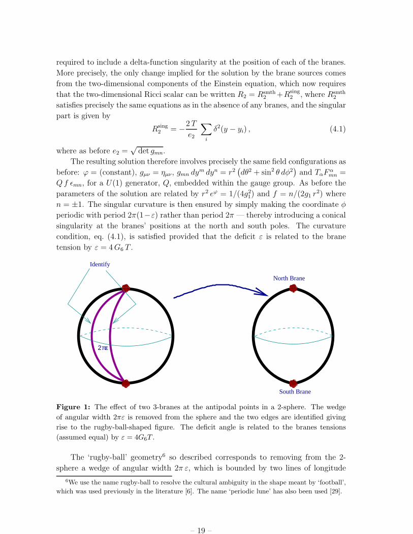
Figure 1: The effect of two 3-branes at the antipodal points in a 2-sphere. The wedge

of angular width 2πε is removed from the sphere and the two edges are identified giving

rise to the rugby-ball-shaped figure. The deficit angle is related to the branes tensions

(assumed equal) by ε = 4G6T .

The ‘rugby-ball’ geometry6 so described corresponds to removing from the 2-

sphere a wedge of angular width 2π ε, which is bounded by two lines of longitude

6We use the name rugby-ball to resolve the cultural ambiguity in the shape meant by ‘football’,

which was used previously in the literature [6]. The name ‘periodic lune’ has also been used [29].

– 19 –

running between the branes at the north and south poles, and then identifying the

edges on either side of the wedge [30, 29, 4, 6]. The delta-function contributions to

R2 are then just what is required to keep the Euler characteristic unchanged, since

χ = − 1

2π

∫

d2y(

Rsmth2 +Rsing

2

)

= 2 . (4.2)

The singular contribution precisely compensates the reduction in the contribution of

the smooth curvature, Rsmth2 , due to the reduced volume of the rugby-ball relative to

the sphere.

Finally, the above configuration also satisfies the equations of motion for the

branes, which state (for constant ϕ or vanishing λ) that they move along a geodesic

according to

ym + Γmpq y

p yq = 0 , (4.3)

where Γmpq is the Christoffel symbol constructed from the 2D metric, gmn. Conse-

quently branes placed precisely at rest anywhere in the two dimensions will remain

there, and this configuration is likely to be marginally stable due to the absence of

local gravitational forces in two spatial dimensions.

4.2 Topological Constraint

We now show that the above solution is further restricted by a topological argument.

This will exclude for instance the possibility of the supersymmetric Salam-Sezgin

compactification in which the monopole background is fully embedded into the ex-

plicit U(1) gauge group factor. But it allows other embeddings, in particular the E6

embedding of [25] that is non-supersymmetric.

In order to make this argument we write the electromagnetic field strength ob-

tained from the field equations as

F =n

2 g1

sin θ dθ ∧ dφ , (4.4)

where n = ±1. The gauge potential corresponding to this field strength can be

chosen in the usual way to be

A± =n

2 g1

[±1 − cos θ] dφ , (4.5)

where the subscript ‘±’ denotes that the configuration is designed to be nonsingular

on a patch which respectively covers the northern or southern hemisphere of the

rugby-ball.

Now comes the main point. A+ and A− must differ by a gauge transformation

on the overlap of the two patches along the equator, and this — with the periodicity

condition φ ≈ φ + 2π (1 − ε) — implies A± must satisfy gA+ − gA− = N dφ/(1 −ε), where N is any integer and g denotes the gauge coupling constant which is

– 20 –

appropriate to the generator Q. In particular g = g6 if Q lies within the E6 subgroup,

as is in ref. [24], or g = g1 if Q corresponds to the explicit U(1) gauge factor, as in

ref. [19]. Notice that this is only consistent with eq. (4.5) if g and g1 are related by

g

g1

=N

n(1 − ε). (4.6)

In particular, g cannot equal g1 if ε 6= 0, and so we cannot choose Q to lie in the

explicit U(1) gauge factor, as for the supersymmetric Salam-Sezgin compactification.

A deeper understanding of this last condition can be had if the 3-brane action is

generalized to include the coupling, eq. (2.5), to the background Maxwell field since

in this case the 3-brane acquires a delta-function contribution to the magnetic flux

of size Q ∝ q. Denoting the flux at the position of each brane by Q±, eq. (4.5)

generalizes to

A± =

[Q±

2π+

n

2g1

(±1 − cos θ)

]

dφ . (4.7)

The same arguments as above then lead to the following generalization of formula

(4.6)Q+ −Q−

2π+n

g1

=N

g(1 − ǫ), (4.8)

which relates the difference, Q+ − Q−, to the integers n and N . This shows that

the constraint we are obtaining is best interpreted as a topological condition on the

kinds of magnetic fluxes which are topologically allowed in order for a solution to

exist (much like the condition that the tensions on each to the two 3-branes must

be equal or, in another context, to the Gauss’ Law requirement that the net charge

must vanish for a system of charges distributed within a compact space). Within

this context eq. (4.6) expresses the conditions which are required in order to have

a solution with Q+ = Q−. Given its topological (long-distance) character, such a

condition is very likely to be preserved under short-distance corrections, and so be

stable under renormalization.7

Although the choice Q+ = Q− precludes a solution with g = g1, it does allow

solutions where Q lies elsewhere in the full gauge group, such as the E6 embedding

above. This model has the great virtue of simplicity, largely due to the constancy

of both the dilaton and the magnetic flux over the two-sphere. It has the drawback

that this simple embedding of the monopole gauge group breaks supersymmetry,

and so may allow larger quantum corrections than would be allowed by the general

arguments of the previous sections. On the other hand, the choice g = g1 may be

possible if Q± are not equal, and if so would allow a solution with unbroken bulk

supersymmetry as in the original Salam-Sezgin model.

7Note added: This stability is easier to see for the single-brane solutions of ref. [48], where it is

very much like the usual quantization of monopole charge.

– 21 –

It clearly would be of great interest to find an anomaly-free embedding that also

preserves some of the supersymmetry, since any such embedding would completely

achieve precisely the scenario we are proposing with a naturally small cosmological

constant. However, although supersymmetry was required to eliminate the contribu-

tions of curvature squared terms, which contribute to ρeff an amount of order M2w/r

2,

we see that even without supersymmetry this model achieves a great reduction in

the cosmological constant relative to the mass-splittings, Mw, between observable

particles and any of their superpartners. A full study of monopole solutions and

their quantum fluctuations is presently being investigated.

5. Conclusions

In this paper we present arguments that supersymmetric six-dimensional theories

with 3-branes can go a long way towards solving the cosmological constant problem.

Unlike most approaches, the arguments we present address (at least partially) both

the high-energy and the low-energy part of the cosmological constant problem: i.e.

why is the cosmological constant so small at high energies and why does it remain

small after integrating out comparatively light degrees of freedom (like the electron)

whose physics we think we understand.

We are motivated to examine six-dimensional theories because of the remarkable

fact that the cosmological constant scale v coincides in these theories with the com-

pactification scale 1/r and the gravitino mass M2w/Mp. This potentially makes the

nonvanishing of the cosmological constant less of a mystery since it becomes related

to the relevant scales of the theory, providing an explanation for the phenomenologi-

cal relationship v ∼M2w/Mp which relates the cosmological constant to the hierarchy

problem. Notice that this relationship would also account for the ‘Why Now?’ prob-

lem — which asks why the Dark Energy should be just beginning to dominate the

Universe at the present epoch — provided the cold dark matter consists of elementary

particles having weak-interaction cross sections [38].

A satisfying consequence of this kind of six-dimensional solution to the cosmo-

logical constant problem is that it shares the many experimental implications of the

sub-millimeter 6D brane scenarios. These are very likely to be testable within the

near future in two distinct ways. First, the scenario predicts violations to Newton’s

gravitational force law at distances below ∼ 0.1 mm, which is close to the edge

of what can be detected. It also predicts the existence of a 6D fundamental scale

just above the TeV scale, and so predicts many forms of extra-dimensional particle

emission and gravitational effects for high-energy colliders. Both predictions pro-

vide a fascinating and unexpected connection between laboratory physics and the

cosmological constant.

We find that self-tuning in 6D supergravity potentially provides a new twist

to the connection between supersymmetry and the cosmological constant. Usually

– 22 –

supersymmetry is thought not to be useful for solving the low-energy part of the

cosmological constant problem since it can at best suppress it to be of order (∆m)4.

The low-energy problem is then how to reconcile this with the absence of observed

superpartners, which requires ∆m >∼ Mw. We overcome this problem by separating

the two scales. No unacceptable superpartners arise for ordinary particles because

particle supermultiplets on the brane are split by O(Mw). Although their contribu-

tion to the vacuum energy is therefore O(M4w), this is not directly a contribution to

the observed 4D cosmological constant because it is localized on the branes and is

cancelled by the contribution of the bulk curvature.

From this point of view the important modes to whose quantum fluctuations

the 4D vacuum energy is sensitive are those in the bulk. But this sector is only

gravitationally coupled, and so in it supersymmetry breaking can really be of or-

der the cosmological constant scale, ∆m ∼ v ∼ 10−3 eV without being imme-

diately inconsistent with observations. We argue here that self-tuning precludes

bulk quantum corrections to the 4D cosmological constant from being larger than

ρeff ∼ M2w/r

2 ∼ M6w/M

2p , making them much smaller than the O(M4

w) contributions

of most 4D supersymmetric theories. Explicit one-loop calculations [27] seem to in-

dicate that the O(M2w/r

2) are also not present for theories where supersymmetry is

broken by boundary conditions, giving a generic zero-point energy (∆m)4, and we

argue qualitatively why this might also be ensured by the self-tuning mechanism.

In this sense our proposal goes beyond explaining why the cosmological constant is

zero, by also explaining why supersymmetry breaking at scale Mw requires it to be

nonzero and of the observed size.

Our proposal shares some features with other brane-based mechanisms which

have been proposed to suppress the vacuum energy after supersymmetry breaking.

For instance, the special role played by supersymmetry in two transverse dimensions

echoes earlier ideas [39] based on (2+1)-dimensional supersymmetry. We regard the

present proposal to be an improvement on the brane-based mechanism of suppressing

the 4D vacuum energy relative to the splitting of masses within supermultiplets

proposed in ref. [40]. This earlier proposal was difficult to embed into an explicit

string model, and required an appeal to negative-tension objects, such as orientifolds,

in order to obtain a small ρeff at high energies. Furthermore, the low-energy part

of the cosmological constant problem was not fully addressed. Our mechanism also

shares some of the features of the self-tuning proposals of [14] in the sense that

flat spacetime is a natural solution of the field equations. But we do not share the

difficulties of that mechanism, such as the unavoidable presence of singularities or

the need for negative tension branes [15, 16].

Our mechanism is most closely related to recent attempts to obtain a small

cosmological constant from branes in non-supersymmetric 6D theories [5, 6]. In par-

ticular we use the special role of 6D to cancel the brane tensions from the bulk

curvature, independent of the value of the tensions. However, our framework goes

– 23 –

beyond theirs in several ways. In the scenarios of [5], the singular part of the Ricci

scalar cancels the contribution from the brane tensions, but the smooth part does

not cancel the other contributions to the cosmological constant, such as a bulk cos-

mological constant. The explicit compactifications considered there, including the

presence of 4-branes, either do not achieve the natural cancellation of the cosmo-

logical constant or have naked singularities. In [6], the same rugby-ball geometry

that we consider was studied in detail. Because of the lack of supersymmetry it was

necessary to tune the value of the bulk cosmological constant to obtain a cancel-

lation with the monopole flux and obtain flat 4D spacetime. Furthermore none of

these proposals address question 2 of our introduction. Our proposal, being based

on supersymmetry, avoids those problems and addresses both questions 1 and 2 of

the introduction.

5.1 Open Questions

Even though our scenario has a number of attractive features, it leaves a great many

questions unanswered.

First, our attempt to realize the self-tuning in an explicit solution to the 6D

equations led to a topological constraint that appears to require a relationship be-

tween the brane tension and other (gauge) couplings in the bulk action. It remains

to be seen whether this condition is an artifact of the simplicity of our solution (such

as being due to our requiring the dilaton and Maxwell fields to be nonsingular at

the brane positions) or if it is actually unavoidably required in order to obtain flat

3-branes. In particular, we argue that the topological relation is better interpreted

as a constraint on what magnetic fluxes which may be carried by the branes given

the topology of the internal space. As such it might be expected to be stable under

renormalization, in much the same way as is the condition that the net electric charge

vanish for a configuration of charged particles in a compact space.

Since the scale of the cosmological constant (and the electroweak/gravitational

hierarchy) is set by r in this picture, it becomes all the more urgent to understand

how the radion can be stabilized at such large values. Six dimensions are promising

in this regard, since they allow several mechanisms for generating potentials which

depend only logarithmically on r [42, 43]. (See ref. [20] for a discussion of stabilization

issues within the 6D Salam-Sezgin model.)

More generally, it is crucial to understand the dynamics of the radion near its

minimum within any such stabilization mechanism, since this can mean that the ra-

dion is even now cosmologically evolving, with correspondingly different implications

for the Dark Energy’s equation of state. Indeed, it has recently been observed that

viable cosmologies based on a sub-millimeter scale radion can be built along these

lines [44].

More precise calculations of the quantum corrections within these geometries

is clearly required in order to sharpen the general order-of-magnitude arguments

– 24 –

presented here. This involves a detailed examination of the full classical solution to

the Einstein-Maxwell-dilaton system in the presence of the branes, as well as the

explicit integration over their quantum fluctuations. Such calculations as presently

exist (both in string theory and field theory [27]) support the claim that the net 4D

vacuum energy density after supersymmetry breaking can be O(1/r4).

At a more microscopic level, it would be very interesting to be able to make

contact with string theory. This requires both a derivation of the effective 6D su-

pergravity theory as a low-energy limit of a consistent string theory (or any other

alternative fundamental theory which may emerge), as well as a way of obtaining

the required types and distributions of branes from a consistent compactification. In

particular it is crucial to check if we can derive the absence of a dilaton coupling to

the branes directly within a stringy context.

One approach is to try to obtain Salam-Sezgin supergravity from within string

theory. As mentioned in [20], the possibility of compactifications based on spheres

[45] in string theory, or fluxes in toroidal or related models [46], could be relevant

to this end. Remembering that the Salam-Sezgin model has a potential which is

positive definite, this may actually require non-compact gaugings and/or duality

twists, such as those recently studied in [47]. Ideally one would like a fully realistic

string model that addresses all of these issues. An alternative approach is to see if our

mechanism generalizes to other 6D supergravities, whose string-theoretic pedigree is

better understood. Work along these lines is also in progress.

A virtue of identifying a low-energy mechanism for controlling the vacuum energy

is that obtaining its realization may be used as a guideline in the search for realistic

string models. This may suggest considering anisotropic string compactifications

with four small dimensions (of order the string scale ∼Mw) and two large dimensions

(r ∼ 0.1 mm) giving rise to a large Planck scale Mp ∼M2wr and a small cosmological

constant Λ ∼ 1/r4 ∼ (M2w/Mp)

4.

All in all, we believe our proposal to be progress in understanding the dark en-

ergy, inasmuch as it allows an understanding of the low-energy — and so also the most

puzzling — part of the problem. We believe these ideas considerably increase the

motivation for studying the other phenomenological implications of sub-millimeter

scale extra dimensions [9], and in particular to the consequences of supersymmetry

in these models [8]. We believe the potential connection between laboratory observa-

tions and the cosmological constant makes the motivation for a more detailed study

of the phenomenology of these models particularly compelling.

Note Added: There have been several interesting developments since this paper

appeared on the arXiv, which we briefly summarize here.

Ref. [41] provide an interesting analysis of the Salam-Sezgin model without

branes, in which they verify the topological condition, eq. (4.6) (as also did ref. [49]),

and show that if the Kaluza-Klein scale is of order 10−3 eV, then the 4D gauge cou-

– 25 –

pling of the bulk gauge fields must be g4 ∼ 10−31 (as opposed to the value of 10−15

which is obtained in the absence of a dilaton [9].). Since this follows directly from

the large size of the extra dimensions, its explanation rests with whatever physics

stabilizes the size of the extra dimensions, and does not represent an additional fine

tuning beyond this. The physics of radius stabilization at such a large value remains

of course an open question.8

Ref. [48] finds the general nonsingular solution to the Salam-Sezgin equations

having maximal symmetry in the noncompact 4 dimensions, for arbitrary monopole

number. These solutions nicely illustrate many of the arguments made here, since

the noncompact 4 dimensions are always flat, as our general self-tuning arguments

predict. The 4D curvature which the field equations require for non-constant dila-

ton is in this case provided by warping in the extra dimensions. Furthermore, the

solutions with monopole number greater than 1 provide examples whose topological

constraints are very plausibly stable against renormalization inasmuch as they closely

resemble the standard monopole quantization condition.

Progress towards embedding our picture into string theory has also been made.

Ref. [50] finds a higher-dimensional derivation of a new supergravity which shares

the bosonic part of the Salam-Sezgin theory. Ref. [51] obtains exactly the Salam-

Sezgin supergravity, by consistently reducing type I/heterotic supergravity on the

non-compact hyperboloid H2,2 times S1.

Finally, ref. [52] provides an explicit recent one-loop string calculation of the vac-

uum energy within a supersymmetry-breaking framework similar to that considered

here. They find a result which is of order 1/r4, in agreement with our arguments

and with previous calculations [27].

Acknowledgments

We thank J. Cline, G. Gibbons, S. Hartnoll and S. Randjbar-Daemi for stimulating

conversations. Y.A. and C.B.’s research is partially funded by grants from McGill

University, N.S.E.R.C. of Canada and F.C.A.R. of Quebec. S.P. and F.Q. are par-

tially supported by PPARC.

References

[1] S. Weinberg, Rev. Mod. Phys. 61 (1989) 1.

8Notational point: We adopt in this paper a slightly different metric convention than we did in

ref. [20] since we here do not work in the 4D Einstein frame. Consequently in this paper KK masses

are of order 1/r instead of being of order geφ/2/r ∼ 1/r2, as they are in ref. [20], and as is shown

explicitly in ref. [41].

– 26 –

[2] S. Perlmutter et al., Ap. J. 483 565 (1997) [astro-ph/9712212]; A.G. Riess et al, Ast.

J. 116 1009 (1997) [astro-ph/9805201]; N. Bahcall, J.P. Ostriker, S. Perlmutter, P.J.

Steinhardt, Science 284 (1999) 1481, [astro-ph/9906463].

[3] For a recent summary of experimental bounds on deviations from General Relativity,

see C.M. Will, Lecture notes from the 1998 SLAC Summer Institute on Particle

Physics [gr-qc/9811036]; C.M. Will[gr-qc/0103036].

[4] F. Leblond, Phys. Rev. D 64 (2001) 045016 [hep-ph/0104273]; F. Leblond,

R. C. Myers and D. J. Winters, JHEP 0107 (2001) 031 [hep-th/0106140].

[5] J.-W. Chen, M.A. Luty and E. Ponton, [hep-th/0003067].

[6] S.M. Carroll and M.M. Guica, [hep-th/0302067]; I. Navarro, [hep-th/0302129].

[7] J. M. Cline, J. Descheneau, M. Giovannini and J. Vinet, [hep-th/0304147].

[8] D. Atwood, C.P. Burgess, E. Filotas, F. Leblond, D. London and I. Maksymyk,

Physical Review D63 (2001) 025007 (14 pages) [hep-ph/0007178].

[9] N. Arkani-Hamed, S. Dimopoulos and G. Dvali, Phys. Lett. B429 (1998) 263

hep-ph/9803315; Phys. Rev. D59 (1999) 086004 [hep-ph/9807344]; I. Antoniadis,

N. Arkani-Hamed, S. Dimopoulos and G. R. Dvali, Phys. Lett. B 436 (1998) 257

[hep-ph/9804398].

[10] Real graviton emission is discussed in G. F. Giudice, R. Rattazzi and J. D. Wells,

Nucl. Phys. B544, 3 (1999) [hep-ph/9811291]; E. A. Mirabelli, M. Perelstein and

M. E. Peskin, Phys. Rev. Lett. 82, 2236 (1999) [hep-ph/9811337]; T. Han,

J. D. Lykken and R. Zhang, Phys. Rev. D59, 105006 (1999) [hep-ph/9811350]; K.

Cheung and W.-Y. Keung, Phys. Rev. D60, 112003 (1999) [hep-ph/9903294]; S.

Cullen and M. Perelstein, Phys. Rev. Lett. 83 (1999) 268 [hep-ph/9903422]; C.

Balazs et al., Phys. Rev. Lett. 83 (1999) 2112 [hep-ph/9904220]; L3 Collaboration

(M. Acciarri et al.), Phys. Lett. B464, 135 (1999), [hep-ex/9909019], Phys. Lett.

B470, 281 (1999) [hep-ex/9910056].

[11] Virtual graviton exchange has also been widely studied, although the interpretation

of these calculations is less clear due to the potential confusion of the results with

the exchange of higher-mass particles [12]. For a review, along with a comprehensive

list of references, see K. Cheung, talk given at the 7th International Symposium on

Particles, Strings and Cosmology (PASCOS 99), Tahoe City, California, Dec 1999,

[hep-ph/0003306].

[12] E. Dudas and J. Mourad, Nucl. Phys. B 575 (2000) 3 [hep-th/9911019];

E. Accomando, I. Antoniadis and K. Benakli, Nucl. Phys. B579, 3 (2000)

[hep-ph/9912287]; S. Cullen, M. Perelstein and M. E. Peskin, [hep-ph/0001166].

[13] S. Cullen and M. Perelstein, Phys. Rev. Lett. 83 (1999) 268 [hep-ph/9903422]; C.

Hanhart, D.R. Phillips, S. Reddy, M.J. Savage, Nucl. Phys. B595 (2001) 335

[nucl-th/0007016].

– 27 –

[14] N. Arkani-Hamed, S. Dimopoulos, N. Kaloper and R. Sundrum, Phys. Lett. B 480

(2000) 193, [hep-th/0001197];

S. Kachru, M. B. Schulz and E. Silverstein, Phys. Rev. D 62 (2000) 045021,

[hep-th/0001206].

[15] S. Forste, Z. Lalak, S. Lavignac and H. P. Nilles, Phys. Lett. B 481 (2000) 360,

hep-th/0002164; JHEP 0009 (2000) 034, [hep-th/0006139].

[16] J.M. Cline and H. Firouzjahi, Phys. Rev. D65 (2002) 043501, [hep-th/0107198].

[17] N. Marcus and J.H. Schwarz, Phys. Lett. 115B (1982) 111.

[18] H. Nishino and E. Sezgin, Phys. Lett. 144B (1984) 187; Nucl. Phys. B 278 (1986)

353.

[19] A. Salam and E. Sezgin, Phys. Lett. 147B (1984) 47.

[20] Y. Aghababaie, C.P. Burgess, S. Parameswaran and F. Quevedo, JHEP 0303 (2003)

032 [hep-th/0212091].

[21] L. Alvarez-Gaume and E. Witten, Nucl. Phys. B234 (1984) 269.

[22] M.B. Green and J.H. Schwarz, Phys. Lett. B149 (1984) 117.

[23] S. Randjbar-Daemi, A. Salam and J. Strathdee, Nucl. Phys. B 214 (1983) 491.

[24] S. Randjbar-Daemi, A. Salam, E. Sezgin and J. Strathdee, Phys. Lett. B151 (1985)

351.

[25] M.B. Green, J.H. Schwarz and P.C. West, Nucl. Phys. B254 (1985) 327; J. Erler, J.

Math. Phys. 35 (1994) 1819 [hep-th/9304104].

[26] S. Weinberg, Gravitation and Cosmology, Wiley, New York, 1972.

[27] See for instance: I. Antoniadis, K. Benakli, A. Laugier and T. Maillard, Nucl. Phys.

B 662 (2003) 40 [arXiv:hep-ph/0211409]; M. Klein, Phys. Rev. D 67 (2003) 045021

[arXiv:hep-th/0209206].

[28] J. Scherk and J.H. Schwarz, Phys. Lett. B82 (1979) 60.

[29] J.S. Dowker, [hep-th/9906067].

[30] S. Deser, R. Jackiw and G. ’t Hooft, Annals Phys. 152 (1984) 220; S. Deser and

R. Jackiw, Annals Phys. 153 (1984) 405.

[31] T. Eguchi, P. B. Gilkey and A. J. Hanson, Phys. Rept. 66 (1980) 213.

[32] D. V. Volkov and V. P. Akulov, Phys. Lett. B 46 (1973) 109. J. Wess and J. Bagger,

“Supersymmetry And Supergravity,” Princeton University press (1992).

– 28 –

[33] See for instance: H. P. Nilles, M. Olechowski and M. Yamaguchi, Nucl. Phys. B 530

(1998) 43 [hep-th/9801030]; E. A. Mirabelli and M. E. Peskin, Phys. Rev. D 58

(1998) 065002 [hep-th/9712214]; E. Dudas and J. Mourad, Phys. Lett. B 514 (2001)

173 [hep-th/0012071]; G. Pradisi and F. Riccioni, Nucl. Phys. B 615 (2001) 33

[arXiv:hep-th/0107090]; I. Antoniadis, K. Benakli and A. Laugier, Nucl. Phys. B

631 (2002) 3 [hep-th/0111209]; M. Klein, Phys. Rev. D 66 (2002) 055009

[hep-th/0205300]; Phys. Rev. D 67 (2003) 045021 [hep-th/0209206]; C. P. Burgess,

E. Filotas, M. Klein and F. Quevedo, [hep-th/0209190].

[34] J.H. Schwarz, Phys. Lett. B371 (1996) 223 [hep-th/9512953]; M. Berkooz, R.G.

Leigh, J. Polchinski, J.H. Schwarz, N. Seiberg and E. Witten, Nucl. Phys. B475

(1996) 115 [hep-th/9605184]; N. Seiberg, Phys. Lett. B390 (1997) 169

[hep-th/9609161].

[35] B. de Wit and J. Louis, [hep-th/9801132].

[36] A. Sagnotti, Phys. Lett. B294 (1992) 196.

[37] M. J. Duff, R. Minasian and E. Witten, Nucl. Phys. B 465 (1996) 413

[hep-th/9601036]; G. Aldazabal, A. Font, L. E. Ibanez and F. Quevedo, Phys. Lett.

B 380 (1996) 33 [hep-th/9602097]; N. Seiberg and E. Witten, Nucl. Phys. B471

(1996) 121 [hep-th/9603003].

[38] N. Arkani-Hamed, L. J. Hall, C. F. Kolda and H. Murayama, Phys. Rev. Lett. 85

(2000) 4434 [astro-ph/0005111].

[39] E. Witten, [hep-th/9409111]; [hep-th/9506101].

[40] C. P. Burgess, R. C. Myers and F. Quevedo, Phys. Lett. B 495 (2000) 384,

[hep-th/9911164]. For similar string constructions see also: I. Antoniadis, E. Dudas

and A. Sagnotti, Phys. Lett. B 464 (1999) 38 [hep-th/9908023]; G. Aldazabal and

A. M. Uranga, JHEP 9910 (1999) 024 [hep-th/9908072].

[41] G. W. Gibbons and C. N. Pope, arXiv:hep-th/0307052.

[42] N. Arkani-Hamed, L. Hall, D. Smith and N. Weiner, Phys.Rev. D62 105002 (2000)

[hep-ph/9912453].

[43] A. Albrecht, C.P. Burgess, F. Ravndal and C. Skordis, Phys. Rev. D65 (2002)

123505 [hep-th/0105261].

[44] A. Albrecht, C.P. Burgess, F. Ravndal and C. Skordis, Phys. Rev. D65 (2002)

123507 [astro-ph/0107573].

[45] See for instance: M. Cvetic, H. Lu and C. N. Pope, Phys. Rev. Lett. 83 (1999) 5226

[hep-th/9906221]; M. Cvetic, H. Lu and C. N. Pope, Nucl. Phys. B 597 (2001) 172

[hep-th/0007109]; M. Cvetic, H. Lu, C. N. Pope, A. Sadrzadeh and T. A. Tran, Nucl.

Phys. B 590 (2000) 233 [hep-th/0005137], and references therein.

– 29 –

[46] See for instance: I. Antoniadis, E. Gava, K. S. Narain and T. R. Taylor, Nucl. Phys.

B 511 (1998) 611 [hep-th/9708075]; T. R. Taylor and C. Vafa, Phys. Lett. B 474

(2000) 130 [hep-th/9912152]; S. Gukov, C. Vafa and E. Witten, Nucl. Phys. B 584

(2000) 69 [Erratum-ibid. B 608 (2001) 477] [hep-th/9906070]; P. Mayr, Nucl. Phys.

B 593 (2001) 99 [hep-th/0003198]; G. Curio, A. Klemm, D. Lust and S. Theisen,

Nucl. Phys. B 609 (2001) 3 [hep-th/0012213]. J. Louis and A. Micu, Nucl. Phys. B

635 (2002) 395 [hep-th/0202168]; D’Auria, S. Ferrara and S. Vaula, New J. Phys. 4

(2002) 71 [hep-th/0206241]; L. Andrianopoli, R. D’Auria, S. Ferrara and

M. A. Lledo, Nucl. Phys. B 640 (2000) 63 [hep-th/0204145].

[47] A. Dabholkar and C. Hull, [hep-th/0210209].

[48] G.W. Gibbons, R. Guven and C.N. Pope, [hep-th/0307238].

[49] I. Navarro, [hep-th/0305014].

[50] J. Kerimo and H. Lu, [hep-th/0307222].

[51] M. Cvetic, G.W. Gibbons and C.N. Pope, [hep-th/0308026].

[52] C. Angelantonj and I. Antoniadis, [hep-th/0307254].

– 30 –