arX

iv:h

ep-t

h/03

1217

0v2

22

Jan

2004

PUPT-2102

Branes, Rings and Matrix Models inMinimal (Super)string Theory

Nathan Seiberg1 and David Shih2

1School of Natural Sciences, Institute for Advanced Study, Princeton, NJ 08540 USA

2Department of Physics, Princeton University, Princeton, NJ 08544 USA

We study both bosonic and supersymmetric (p, q) minimal models coupled to Liouville

theory using the ground ring and the various branes of the theory. From the FZZT brane

partition function, there emerges a unified, geometric description of all these theories in

terms of an auxiliary Riemann surface Mp,q and the corresponding matrix model. In terms

of this geometric description, both the FZZT and ZZ branes correspond to line integrals of

a certain one-form on Mp,q. Moreover, we argue that there are a finite number of distinct

(m,n) ZZ branes, and we show that these ZZ branes are located at the singularities of

Mp,q. Finally, we discuss the possibility that the bosonic and supersymmetric theories

with (p, q) odd and relatively prime are identical, as is suggested by the unified treatment

of these models.

December, 2003

1. Introduction and conclusions

In this work we will explore minimal string theories. These are simple examples of

string theory with a small number of observables. Their simplicity makes them soluble

and therefore they are interesting laboratories for string dynamics.

The worldsheet description of these minimal string theories is based on the (p, q)

minimal conformal field theories coupled to two-dimensional gravity (Liouville theory), or

the (p, q) minimal superconformal field theories coupled to two-dimensional supergravity

(super-Liouville theory). Even though these two worldsheet descriptions appear different,

we find that actually they are quite similar. In fact, our final answer depends essentially

only on the values of (p, q). This suggests a uniform presentation of all these theories which

encompasses the two different worldsheet frameworks and extends them.

These theories were first solved using their description in terms of matrix models [1-8]

(for reviews, see e.g. [9,10]). The matrix model realizes the important theme of open/closed

string duality in the study of string theory. Recent advances in the study of Liouville theory

[11-13] and its D-branes [14-16] has led to progress by [17-24] and others in making the

connection between the matrix model and the worldsheet description more explicit. Much

of the matrix model treatment of these theories has involved a deformation by the lowest

dimension operator. In order to match with the worldsheet description based on Liouville

theory, we should instead tune the background such that only the cosmological constant

µ is turned on. In [25] such backgrounds were referred to as conformal backgrounds.

In the first part of this work, we will examine the simplest examples of minimal string

theory, which are based on the bosonic (p, q) minimal models coupled to two-dimensional

gravity. These theories, which we review in section 2, exist for all relatively prime integers

(p, q). It is important that these theories have only a finite number of standard physical

vertex operators Tr,s of ghost number one; we will refer to these as tachyons. They are

constructed by “dressing” the minimal model primaries Or,s with Liouville exponentials,

subject to the condition that the combinations have conformal dimension one. They are

labelled by integers r = 1, . . . , p − 1 and s = 1, . . . , q − 1, and they are subject to the

identification Tr,s ∼ Tp−r,q−s, which can be implemented by restricting to qr > ps.

In addition to the tachyons, there are infinitely many physical operators at other values

of the ghost number [26]. Of special importance are the operators at ghost number zero.

These form a ring [27] under multiplication by the operator product expansion modulo

1

BRST commutators. We will argue that the ring is generated by two operators O1,2 and

O2,1. In terms of the operators

x =1

2O1,2 , y =

1

2O2,1 , (1.1)

the other elements in the ring are

Or,s = Us−1(x)Ur−1(y) (1.2)

where the U are the Chebyshev polynomials of the second kind Ur−1(cos θ) = sin(rθ)sin θ and

for simplicity we are setting here the cosmological constant µ = 1. The ring has only

(p− 1)(q − 1) elements. The restriction on the values of (r, s) is implemented by the ring

relations

Uq−1(x) = 0 , Up−1(y) = 0 . (1.3)

The tachyons Tr,s form a module of the ring, which is simply understood by writing

Tr,s = Or,sT1,1. The restriction in the tachyon module rq > ps implies that the module

is not a faithful representation of the ring. Instead, there is an additional relation in the

ring when acting on the tachyon module:

(Uq−2(x) − Up−2(y)

)Tr,s = 0 . (1.4)

The ground ring will enable us to compute some simple correlation functions such as

〈Tr1,s1Tr2,s2

Tr3,s3〉 = N(r1,s1)(r2,s2)(r3,s3)〈T1,1T1,1T1,1〉 (1.5)

with N(r1,s1)(r2,s2)(r3,s3) the integer fusion rules of the minimal model.

In sections 3 and 4, we study the two types of branes in these theories, which are

referred to as the FZZT and ZZ branes [14-16]. The former were previously explored

in the context of matrix models as operators that create macroscopic loops [28,25,29,30].

The Liouville expressions for these loops [14,15] lead to more insight. The general Liouville

expressions simplify in our case for two reasons. First, the Liouville coupling constant b2

is rational, b2 = pq; and second, we are not interested in the generic Liouville operator

but only in those which participate in the physical (i.e. BRST invariant) operators of

the minimal string theory. It turns out that these branes are labelled by a continuous

parameter x which can be identified with the boundary cosmological constant µB . This

2

parameter can be analytically continued, but it does not take values on the complex plane.

Rather, it is defined on a Riemann surface Mp,q which is given by the equation

F (x, y) ≡ Tq(x) − Tp(y) = 0 (1.6)

with Tp(cos θ) = cos(p θ) a Chebyshev polynomial of the first kind. This Riemann surface

has genus zero, but it has (p− 1)(q − 1)/2 singularities that can be thought of as pinched

A-cycles of a higher-genus surface. In addition to (1.6), the singularities must satisfy

∂xF (x, y) = q Uq−1(x) = 0

∂yF (x, y) = pUp−1(y) = 0 .(1.7)

Rewriting the conditions (1.6) and (1.7) as

Uq−1(x) = Up−1(y) = 0

Uq−2(x) − Up−2(y) = 0 ,(1.8)

we immediately recognize the first line as the ring relations (1.3), and the second line as

the relation in the tachyon module (1.4).

Deformations of the curve (1.6) correspond to the physical operators of the minimal

string theory. Among them we find all the expected bulk physical operators, namely the

tachyons, the ring elements and the physical operators at negative ghost number. There

are also deformations of the curve that do not correspond to bulk physical operators. We

interpret these to be open string operators.

A useful object is the one form y dx. Its integral on Mp,q from a fixed reference point

(which we can take to be at x → ∞) to the point µB is the FZZT disk amplitude with

boundary cosmological constant µB:

Z(µB) =

∫ µB

y dx . (1.9)

We can also consider closed contour integrals of this one-form through the pinched cycles

of Mp,q. This leads to disk amplitudes for the ZZ branes:

Zm,n =

∮

Bm,n

y dx . (1.10)

This integral can also be written as the difference between FZZT branes on the two sides

of the singularity [24]. Such a relation between the two types of branes follows from the

work of [16,31,32] and was made most explicit in [18].

3

The relations (1.8) which are satisfied at the singularities, together with the result

(1.10), suggest the interpretation of the (m,n) ZZ brane states as eigenstates of the ring

generators x and y, with eigenvalues xmn and ymn corresponding to the singularities of

Mp,q:

x|m,n〉ZZ = xmn|m,n〉ZZ , y|m,n〉ZZ = ymn|m,n〉ZZ . (1.11)

We also find that these eigenvalues completely specify the BRST cohomology class of the ZZ

brane. In other words, branes located at the same singularity of Mp,q differ by a BRST

exact state, while branes located at different singularities are distinct physical states.

Moreover, branes that do not correspond to singularities of our surface are themselves

BRST exact. Thus there are as many distinct ZZ branes as there are singularities of Mp,q

in (p, q) minimal string theory.

A natural question is the physical interpretation of the uniformization parameter θ of

our surface, defined by x = cos θ. The answer is given in appendix A, where we discuss the

(nonlocal) Backlund transformation that maps the Liouville field φ to a free field φ. We

will see that θ can be identified with the Backlund field, which satisfies Dirichlet boundary

conditions.

In the second part of our paper we will study the minimal superstring theories, which

are obtained by coupling (p, q) superminimal models to supergravity. These theories fall

in two classes. The odd models exist for p and q odd and relatively prime. They (spon-

taneously) break worldsheet supersymmetry. The even models exist for p and q even, p/2

and q/2 relatively prime and (p − q)/2 odd. Our discussion parallels that in the bosonic

string and the results are very similar. There are however a few new elements.

The first difference from the bosonic system is the option of using the 0A or 0B GSO

projection. Most of our discussion will focus on the 0B theory. In either theory, there is a

global Z2 symmetry (−1)FL , where FL is the left-moving spacetime fermion number. This

symmetry multiplies all the RR operators by −1 and is broken when background RR fields

are turned on. Orbifolding the 0B theory by (−1)FL leads to the 0A theory and vice versa.

A second important difference relative to the bosonic system is that here the cos-

mological constant µ can be either positive or negative, and the results depend on its

sign

ζ = sign(µ) . (1.12)

This sign can be changed by performing a Z2 R-transformation in the super-Liouville part

of the theory. It acts there as (−1)fL with fL the left moving worldsheet fermion number.

4

Since this is an R-transformation, it does not commute with the worldsheet supercharge.

In order to commute with the BRST charge such an operation must act on the total

supercharge including the matter part. This operation is usually not a symmetry of the

theory. In particular it reverses the sign of the GSO projection in the Ramond sector.

Therefore, our answers will in general depend on ζ.

In section 5 we discuss the tachyons, the ground ring and the correlation functions.

The results are essentially identical to those in the bosonic string except that we should use

the appropriate values of (p, q), and the ring relation in the tachyon module (1.4) depends

on ζ(Uq−2(x) − ζUp−2(y)

)Tr,s = 0 . (1.13)

In sections 6 and 7 we consider the supersymmetric FZZT and ZZ branes. Here we find a

third element which is not present in the bosonic system. Now there are two kinds of branes

labelled by a parameter η = ±1; this parameter determines the combination of left and

right moving supercharges that annihilates the brane boundary state: (G+ iηG)|B〉 = 0.

We must also include another label ξ = ±1 which multiplies the Ramond component of

the boundary state. It is associated with the Z2 symmetry (−1)FL . Changing the sign of

ξ maps a brane to its antibrane.

Most of these new elements do not affect the odd models. The answers are independent

of ζ and η, and we again find the Riemann surface Mp,q given by the curve Tq(x)−Tp(y) =

0. The characterization of the FZZT and ZZ branes as contour integrals of y dx is identical

to that in the bosonic string.

The even models are richer. Here we find two Riemann surfaces Mηp,q depending on

the sign of

η = ζη . (1.14)

These surfaces are described by the curves

Fη(x, y) = Tq(x) − η Tp(y) = 0 . (1.15)

The discussion of the surface M−p,q is similar to that of the bosonic models. The surface

M+p,q is more special, because it splits into two separate subsurfaces T p

2(y) = ξT q

2(x) which

touch each other at singular points. The two subsurfaces are interpreted as associated

with the choice of the Ramond “charge” ξ = ±1. The two kinds of FZZT branes which

are labelled by ξ correspond to line integrals from infinity in the two sub-surfaces. ZZ

branes are again given by contour integrals. These can be either closed contours which

5

pass through the pinched singularities in each subsurface, or they can be associated with

contour integrals from infinity in one subsurface through a singularity which connects the

two subsurfaces to infinity in the other subsurface.

It is surprising that our results depend essentially only on p and q. The main differ-

ence between the bosonic models and the supersymmetric models is in the allowed values

of (p, q). Odd p and q which are relatively prime occur in both the bosonic and the su-

persymmetric models. This suggests that these two models might in fact be the same.

This suggestion is further motivated by the fact that the two theories have the same KPZ

scalings [24,33]. Indeed, all our results for these models (ground ring, sphere three point

function, FZZT and ZZ branes) are virtually identical. We will discuss the evidence for

the equivalence of these models in section 8.

Our work goes a long way to deriving the matrix model starting from the worldsheet

formulation of the theory. We will discuss the comparison with the matrix model in section

9. Our Riemann surface Mp,q occurs naturally in the matrix model and determines the

eigenvalue distribution. Of all the possible matrix model descriptions of the minimal string

theories, the closest to our approach are Kostov’s loop gas model [30-37] and the two matrix

model [38], in which expressions related to ours were derived. For the theories with p = 2,

we also have a description in terms of a one-matrix model. Some more detailed aspects of

the comparison to the one-matrix model are worked out in appendix B.

The matrix model also allows us to explore other values of (p, q) which are not on

the list of (super)minimal models. For example, the theories with (p, q) = (2, 2k+ 2) were

interpreted in [24] as a minimal string theory with background RR fields. It is natural to

conjecture that all values of (p, q) correspond to some minimal string theory or deformations

thereof. This generalizes the worldsheet constructions based on (super)minimal models and

(super)Liouville theory.

The Riemann surface which is central in our discussion is closely related to the target

space of the eigenvalues of the matrix model. However, it should be stressed that neither

the eigenvalue direction nor the Riemann surface are the target space of the minimal

string theory itself. Instead, the target space is the Liouville direction φ, which is related

to the eigenvalue space through a nonlocal transform [29]. This distinction between φ and

the coordinates of the Riemann surface is underscored by the fact that x and y on the

Riemann surface are related to composite operators in the worldsheet theory (the ground

ring generators), rather than to the worldsheet operator φ.

6

Our discussion is limited to the planar limit, where the worldsheet topology is a sphere

or a disk (with punctures). It would be interesting to extend it to the full quantum string

theory. It is likely that the work of [39,40] is a useful starting point of this discussion.

A crucial open problem is the nonperturbative stability of these theories. For instance,

some of the bosonic (p, q) theories are known to be stable while others are known to be

unstable. In fact, as we will discuss in section 9, the matrix model of all these models

have a small instability toward the tunnelling of a small number of eigenvalues. The

nonperturbative status of models based on generic values of (p, q) remains to be understood.

After the completion of this work an interesting paper [41] came out which overlaps

with some of our results and suggests an extension to the quantum string theory.

2. Bosonic minimal string theory

2.1. Preliminaries

We start by summarizing some relevant aspects of the (p, q) minimal models and

Liouville theory that we will need for our analysis, at the same time establishing our

notations and conventions. For the bosonic theories, we will take α′ = 1. The (p, q)

minimal models exist for all p, q ≥ 2 coprime. Our convention throughout will be p < q.

The central charge of these theories is given by

c = 1 − 6(p− q)2

p q(2.1)

The (p, q) minimal model has a total of Np,q = (p − 1)(q − 1)/2 primary operators Or,s

labelled by two integers r and s, with r = 1, . . . , p− 1 and s = 1, . . . , q − 1. They satisfy

the reflection relation Op−r,q−s ≡ Or,s and have dimensions

∆(Or,s) = ∆(Or,s) =(rq − sp)2 − (p− q)2

4p q. (2.2)

In general the operator Or,s contains two primitive null vectors among its conformal de-

scendants at levels rs and (p− r)(q − s). Because they are degenerate, primary operators

must satisfy the fusion rules

Or1,s1Or2,s2

=∑

[Or,s]

r = |r1 − r2| + 1, |r1 − r2| + 3, . . . ,

min(r1 + r2 − 1, 2p− 1 − r1 − r2)

s = |s1 − s2| + 1, |s1 − s2| + 3, . . . ,

min(s1 + s2 − 1, 2q − 1 − s1 − s2)

(2.3)

7

The fusion of any operator with O1,2 and O2,1 is especially simple:

O1,2Or,s = [Or,s+1] + [Or,s−1]

O2,1Or,s = [Or+1,s] + [Or−1,s] .(2.4)

Thus in a sense, O1,2 and O2,1 generate all the primary operators of the minimal model.

In particular, O1,2 generates all primaries of the form O1,s and O2,1 generates all primaries

of the form Or,1. The fusion of two such operators is very simple: O1,sOr,1 = [Or,s].

The central charge of Liouville field theory is

c = 1 + 6Q2 = 1 + 6

(b+

1

b

)2

(2.5)

where Q = b + 1b is the background charge. The basic primary operators of the Liouville

theory are the vertex operators Vα = e2αφ with dimension

∆(α) = ∆(α) = α(Q− α) . (2.6)

Of special interest are the primaries in degenerate Virasoro representations

Vαr,s= e2αr,sφ, 2αr,s =

1

b(1 − r) + b(1 − s) . (2.7)

For generic b, these primaries have exactly one singular vector at level rs. Therefore, their

irreducible character is given by:

χr,s(q) =q∆(αr,s)−(c−1)/24

η(q)(1 − qrs) (2.8)

The degenerate primaries also satisfy the analogue of the minimal model fusion rule (2.4)

[11,13]:

V− b2Vα = [Vα− b

2] + C(α)[Vα+ b

2]

C(α) = −µπγ(2bα− 1 − b2)

γ(−b2)γ(2bα)

(2.9)

with a similar expression for V− 12b

:

V− 12bVα = [Vα− 1

2b] + C(α)[Vα+ 1

2b]

C(α) = −µπγ(2α/b− 1 − 1/b2)

γ(−1/b2)γ(2α/b).

(2.10)

8

Here γ(x) = Γ(x)/Γ(1−x). Notice that the second OPE may be obtained from the first by

taking b → 1/b and also µ → µ. The quantity µ is the dual cosmological constant, which

is related to µ via πµγ(1/b2) = (πµγ(b2))1/b2 . From this point onwards, we will find it

convenient to rescale µ and µ so that

µ = µ1/b2 . (2.11)

This will simply many of our later expressions.

In order to construct a minimal string theory, we must couple the (p, q) minimal model

to Liouville. Demanding the correct total central charge implies that the Liouville theory

must have

b =

√p

q. (2.12)

We will see throughout this work that taking b2 to be rational and restricting only to the

BRST cohomology of the full string theory gives rise to many simplifications, and also

to a number of subtleties. One such a simplification is that not all Liouville primaries

labelled by α correspond to physical (i.e. BRST invariant) vertex operators of minimal

string theory. For instance, physical vertex operators may be formed by first “dressing”

an operator Or,s from the matter theory with a Liouville primary Vβr,ssuch that the

combination has dimension (1, 1), and then multiplying them with the ghosts cc. We will

refer to such operators as “tachyons.” Requiring the sum of (2.2) and (2.6) to be 1 gives

the formula for the Liouville dressing of Or,s:

Tr,s = ccOr,sVβr,s

2βr,s =p+ q − rq + sp√

p q, rq − sp ≥ 0 .

(2.13)

Note that in solving the quadratic equation for βr,s, we have chosen the branch of the

square root so that βr,s < Q/2 [42].

An important subtlety that arises at rational b2 has to do with the irreducible character

of the degenerate primaries. The formula (2.8) that we gave above for generic b must now

be modified for a number of reasons.1

1 We thank B. Lian and G. Zuckerman for helpful discussions about the structure of these

representations.

9

1. Different (r, s) can now lead to the same degenerate primary, and therefore labelling

the representations with (r, s) is redundant. It will sometimes be convenient to remove

this redundancy by defining

N(t,m, n) ≡ | tpq +mq + np | (2.14)

and labelling each representation by (t,m, n) satisfying

0 < m ≤ p , 0 < n ≤ q , t ≥ 0 (2.15)

such that the degenerate primary has dimension

∆(t,m, n) =(p+ q)2 −N(t,m, n)2

4pq(2.16)

Then each (t,m, n) satisfying (2.15) corresponds to a unique degenerate representation

and vice versa.

2. The Verma module of a degenerate primary can now have more than one singular

vector. For instance, we can write

N(t,m, n) = ((t− j)p+m)q + (jq + n)p (2.17)

for j = 0, . . . , t, and by continuity in b we expect the Verma module of (t,m, n) to

contain singular vectors at levels ((t− j)p+m)(jq + n), with dimensions

∆ =(p+ q)2 −N(t− 2j,m,−n)2

4pq(2.18)

3. A related subtlety is that a singular vector can itself be degenerate. For example, the

singular vectors discussed above are degenerate as long as t− 2j 6= 0. In general, this

will lead to a complicated structure of nested Verma submodules contained within

the original Verma module of the degenerate primary. A similar structure is seen, for

instance, in the minimal models at c < 1. An important distinction is that here there

are only finitely many singular vectors.

Taking into account these subtleties leads to a formula for the character slightly more

complicated than the naive formula (2.8). The answer is [43,44]:

χt,m,n(q) =1

η(q)

t∑

j=0

(q−N(t−2j,m,n)2/4pq − q−N(t−2j,m,−n)2/4pq

)(2.19)

10

Notice that we can also write this as a sum over naive characters (2.8):

χt,m,n(q) =

[ t2 ]∑

j=0

χ(t−2j)p+m,n −[ t−1

2 ]∑

j=0

χ(t−2j)p−m,n (2.20)

For t = 0, the formula reduces to (2.8), i.e. χt=0,m,n = χm,n. These results will be

important when we come to discuss the ZZ boundary states of minimal string theory in

section 3.

2.2. The ground ring of minimal string theory

The other important collection of BRST invariant operators in minimal string theory

is the ground ring of the theory. The ground ring consists of all dimension 0, ghost number

0, primary operators in the BRST cohomology of the theory [26], and it was first studied

for the c = 1 bosonic string in [27]. Ring multiplication is provided by the OPE modulo

BRST commutators. As in the matter theory, elements Or,s of the ground ring are labelled

by two integers r and s, r = 1, . . . , p − 1 and s = 1, . . . , q − 1. In contrast to the matter

primaries, however, Or,s and Op−r,q−s are distinct operators. Thus the ground ring has

(p− 1)(q − 1) elements, twice as many as the matter theory.

The construction of the ground ring starts by considering the combination Or,sVαr,s

of a matter primary and a corresponding degenerate Liouville primary. Using (2.2) and

(2.6), it is easy to see that this combination has dimension 1−rs. Acting on Or,sVαr,swith

a certain combination of level rs− 1 raising operators then gives the ground ring operator

Or,s = Lr,s · Or,sVαr,s, 2αr,s =

p+ q − rq − sp√pq

. (2.21)

From the construction, it is clear that Or,s has Liouville momentum 2αr,s. When b and

1/b are incommensurate (which is the case for the (p, q) minimal models), (2.21) then

implies that there is a unique ground ring operator at a given Liouville momentum 2αr,s

for r = 1, . . . , p − 1 and s = 1, . . . , q − 1. It follows that the multiplication table for the

ground ring can be derived from kinematics alone. When µ = 0, Liouville momentum is

conserved in the OPE, and therefore one must have

Or,s = Os−11,2 Or−1

2,1 . (2.22)

11

Thus the ground ring is generated by two elements, O1,2 and O2,1. Moreover, the fact that

the ring has finitely many elements leads to non-trivial relations for the ring generators:

Oq−11,2 = 0

Op−12,1 = 0 .

(2.23)

Both (2.22) and (2.23) (and all the ground ring equations that follow) are understood to

be true modulo BRST commutators.

Using the µ-deformed Liouville OPEs (2.9), (2.10) it is easy to see how ring multi-

plication and the ring relations are altered at µ 6= 0. It will be convenient to define the

dimensionless combinations

x =1

2õO1,2, y =

1

2õO2,1 . (2.24)

Let us start by analyzing the operators Or,1. It is clear that Or,1 = Pr−1(y) is a polynomial

of degree r − 1 in the generator y. These polynomials are constrained by the fusion rules

Pr−1(y)Pl−1(y) =∑

ar,l,kPk−1(y)

k = |r − l| + 1, |r − l| + 3, . . . ,

min(r + l − 1, 2p− 1 − r − l)

(2.25)

The restrictions on the sum in (2.25) determine most of the coefficients in Pr−1 even

without using the known values of the operator product coefficients ((2.9) and the similar

coefficient in the minimal model).2 The remaining coefficients can be computed using the

OPE in the minimal model and Liouville, but we will not do that here. Instead we will

simply state the answer. We claim that

Or,1 = µq(r−1)

2p Ur−1(y) (2.26)

where the U are Chebyshev polynomials of the second kind. We will postpone the full

justification of our claim until we come to discuss the ZZ brane one-point functions in

2 For example, all the coefficients in Pr and all the coefficients ar,l,k in (2.25) are determined

in terms of a1,r,r−1 which appears in P1(y)Pr(y) = Pr+1(y)+ a1,r,r−1Pr+1(y). The p-dependence

of the truncation of the sum in (2.25) leads to the ring relation Pp−1(y) = 0, which generalizes

(2.23) to nonzero µ, and leads to relations among the coefficients a1,r,r−1.

12

section 3.1. Also, the computation of the tachyon three-point functions below will provide

a non-trivial check of (2.26).

For now, let us simply show that our ansatz is consistent with (2.25). This is a result

of the following trigonometric identity for the multiplication of the Chebyshev polynomials

U :Ur−1(y)Ul−1(y) =

∑

k

Uk−1(y)

k = |r − l| + 1, |r − l| + 3, . . . , r + l − 1 .

(2.27)

The fact that the Chebyshev polynomials can be expressed as SU(2) characters

Ur−1(cos θ) =sin(rθ)

sin θ= Trj= r−1

2e2iθJ3 . (2.28)

underlies the identity (2.27). This identity is almost of the form (2.25). The p-dependence

in (2.25) is implemented by the ring relation

Up−1(y) = 0 . (2.29)

(This is a standard fact in the representation theory of SU(2).) This shows that the

expression (2.26) with the relation (2.29) satisfies (2.25) with all nonzero ar,l,k equal to

one.

It is trivial to extend these results to the operators O1,s which are generated by x.

Finally, using Or,s = Or,1O1,s we derive the expressions for the ring elements

Or,s = µq(r−1)+p(s−1)

2p Us−1(x)Ur−1(y) (2.30)

and the relationsUq−1(x) = 0

Up−1(y) = 0 .(2.31)

Having found the ring multiplication, we can use it to analyze the tachyon operators

(2.13). Ghost number conservation implies that the tachyons are a module of the ring [45].

Using our explicit realization in terms of the generators (2.30) it is clear that

Tr,s = µ1−sOr,sT1,1 = µq(r−1)−p(s−1)

2p Us−1

(x)Ur−1

(y)T1,1 . (2.32)

Using this expression it is easy to act on Tr,s with any ring operator. This can be done

by writing the ring operator and the tachyon in terms of the generators as in (2.30) and

13

(2.32) and then simply multiplying the polynomials in the generators subject to the ring

relations (2.31).

It is clear, however, that this cannot be the whole story. There are (p − 1)(q − 1)

different ring elements Or,s, but there are only (p− 1)(q− 1)/2 tachyons Tr,s because they

are subject to the identification

Tp−r,q−s = µps−qr

p Tr,s . (2.33)

This means that in addition to the two ring relations (2.31) there must be more relations

which are satisfied only in the tachyon module; i.e. it is not a faithful representation of the

ring. It turns out that one should impose

(Uq−2(x) − Up−2(y)

)Tr,s = 0 . (2.34)

It is easy to show, using trigonometric/Chebyshev identities, that this relation guarantees

the necessary identifications [46] (see also [47,48]). Note that equation (2.34) can also be

written using the ring relations (2.31) in terms of the Chebyshev polynomials of the first

kind Tp(x) = cos(p θ) as(Tq(x) − Tp(y)

)Tr,s = 0 . (2.35)

This expression will be useful in later sections. We should also point out that the effect

of the relations (2.31) and (2.34) on ring multiplication is to truncate it to precisely the

fusion rules (2.3) of the minimal model.

Using this understanding we can constrain the correlation functions of these operators.

The simplest correlation functions involve three tachyons and any number of ring elements

on the sphere. Because of the conformal Killing vectors on the sphere, this calculation

does not involve any moduli integration. It is given by

〈Tr1,s1Tr2,s2

Tr3,s3

∏

i≥4

Ori,si〉 = µ3−s1−s2−s3〈T1,1T1,1T1,1

∏

i≥1

Ori,si〉 . (2.36)

The product of ring elements can be recursively simplified using the ring relations (2.31)

and (2.34). This leads to a linear combination of ring elements, of which only O1,1 survives

in the expectation value (2.36). As an example, consider the three-point function:

〈Tr1,s1Tr2,s2

Tr3,s3〉 = µ3−s1−s2−s3〈T1,1T1,1T1,1Or1,s1

Or2,s2Or3,s3

〉

= N(r1,s1)(r2,s2)(r3,s3)µκ

(2.37)

14

where N(r1,s1)(r2,s2)(r3,s3) ∈ {0, 1} represent the integer fusion rules of the conformal field

theory and κ is the KPZ exponent of the correlation function:

κ =Q−

∑i βri,si

b. (2.38)

Note that in calculating the three-point function, we have normalized 〈T 31,1〉 = µ

Q

b−3.

The surprising result that the three-point functions are given simply by the mini-

mal model fusion rules was noticed many years ago using different methods [49-51]. The

agreement between our calculation and the results in [49-51] serves as a check of our ansatz

(2.30) for the µ-deformed ring multiplication. (We will also give an independent derivation

of (2.30) in section 3.1 using the ZZ branes.) From our current perspective, the simplic-

ity of the tachyon three-point functions follows from the simplicity of the expressions for

the ring elements (2.30) and the relations (2.31), (2.34). At a superficial level we can

view the minimal string theory as a topological field theory based on the chiral algebra

V irasoro/V irasoro. Its physical operators are the primaries of the conformal field theory

and its three point functions are the fusion rule coefficients.

For correlation functions involving fewer than three tachyons we simply insert the

necessary power of the cosmological constant T1,1 in order to have three tachyons. Then

we integrate with respect to µ to find the desired two- or one-point functions.

It would be nice to generalize this method to four and higher-point correlation func-

tions. For such correlators, there are potential complications involving contact terms

between the integrated vertex operators.

3. FZZT and ZZ branes of minimal string theory

3.1. Boundary states and one-point functions

In this section, we will study in detail the FZZT and ZZ branes of Liouville theory

coupled to the bosonic (p, q) minimal models. Let us first review what is known about

the FZZT and ZZ boundary states in these theories. To make the former, we must tensor

together an FZZT boundary state in Liouville and a Cardy state from the matter. This

gives the boundary state [14,15,52]:

|σ; k, l〉 =∑

k′,l′

∫ ∞

0

dP cos(2πPσ)Ψ∗(P )S(k, l; k′, l′)√

S(1, 1; k′, l′)|P 〉〉L|k′, l′〉〉M . (3.1)

15

Here (k, l) labels the matter Cardy state associated to the minimal model primary Ok,l and

|p〉〉L and |k′, l′〉〉M are Liouville and matter Ishibashi states, respectively. The Liouville

and matter wavefunctions are cos(2πP σ)Ψ(P ) and S(k, l; k′, l′), where

Ψ(P ) = µ− iPb

Γ(1 + 2iP

b

)Γ(1 + 2iP b)

iπP

S(k, l; k′, l′) = (−1)kl′+k′l sin(πpll′

q) sin(

πqkk′

p) .

(3.2)

The matter wavefunction is essentially the modular S-matrix of the minimal model. Note

that we have separated out the σ dependent part of the Liouville wavefunction for later

convenience. Finally, the parameter σ is related to the boundary cosmological constant

µB via3

µB√µ

= coshπbσ . (3.3)

By thinking of the FZZT states as Liouville analogues of Cardy states, one also finds

that the state labelled by σ is associated to the non-degenerate Liouville primary with

2α = Q+ iσ [16].

Using the expression (3.1) for the FZZT boundary state, we can easily calculate the

one-point functions of physical operators on the disk with the FZZT boundary condition.

Let us start with the physical tachyon operators Tr,s = Or,se2βr,sφ with βr,s defined in

(2.13). Using P = i(Q/2 − βr,s) in (3.1), we find

〈Tr,s| σ; k, l〉 = Ar,s(−1)ks+lr cosh

(π(qr − ps)σ√

pq

)sin(

πqkr

p) sin(

πpls

q) (3.4)

where the (σ, k, l) independent normalization factor Ar,s will be irrelevant for our purposes.

We can similarly compute the one-point functions for the ground ring elements Or,s.

As discussed in section 2, these take the general form

Or,s = Lr,s · Or,se2αr,sφ (3.5)

where Lr,s denotes a certain combination of Virasoro raising operators of total level rs−1.

These only serve to contribute an overall (σ, k, l) independent factor to the one-point

3 We have rescaled the usual definition of µB, together with the rescaling of µ that we men-

tioned above (2.11). Our conventions for µ and µB relative to, e.g. [14], are µhere = πµthereγ(b2)

and (µB)here = (µB)there

√πγ(b2) sinπb2.

16

functions. Since αr,s = βr,−s, the ground ring ring one-point functions are identical to the

tachyon one-point functions (3.4) up to normalization.

Finally, let us consider the physical operators at negative ghost number [26].4 These

are essentially copies of the ground ring, and their construction is analogous to (3.5).

Their Liouville momentum is also given by βr,s, but with s taking the values s < −q and

s 6= 0 mod q. Thus their one-point functions will also be given by (3.4) up to normalization,

with the appropriate values of s.

The tachyons, the ground ring, and the copies of the ground ring at negative ghost

number are the complete set of physical operators in the minimal string theory. Their

one-point functions (3.4) have several interesting properties as functions of (σ, k, l). First,

they satisfy an identity relating states with arbitrary matter label to states with matter

label (k, l) = (1, 1)

〈O| σ;k, l〉 =∑

m′,n′

〈O| σ +i(m′q + n′p)√

pq; 1, 1〉 (3.6)

with (m′, n′) ranging over the values

m′ = −(k − 1),−(k − 1) + 2, . . . , k − 1

n′ = −(l − 1),−(l − 1) + 2, . . . , l− 1 .(3.7)

Here O stands for an arbitrary physical operator. This is evidence that in the full string

theory, where the boundary states are representatives of the BRST cohomology, the fol-

lowing is true

| σ;k, l〉 =∑

m′,n′

| σ +i(m′q + n′p)√

pq; 1, 1〉 (3.8)

modulo BRST exact states. We should emphasize that (3.8), which relates branes with

different matter states, is an inherently quantum mechanical result. This relation is difficult

to understand semiclassically, where branes with different matter states appear distinct.

But there is no contradiction, because (3.8) involves a shift of σ by an imaginary quantity,

which amounts to analytic continuation of µB from the semiclassical region where it is real

and positive.

4 In some of the literature, physical operators at positive ghost number are also discussed.

However, these violate the Liouville bound α < Q/2 [42]. Thus they are not distinct from the

negative ghost number operators, but are related by the reflection α → Q − α.

17

According to (3.8), the FZZT branes with (k, l) = (1, 1) form a complete basis of all

the FZZT branes of the theory. The branes with other matter states should be thought

of as multi-brane states formed out of these elementary FZZT branes. This allows us to

simplify our discussion henceforth by restricting our attention, without loss of generality,

to the elementary FZZT (and ZZ) branes with (k, l) = (1, 1). We will also simplify the

notation by dropping the label (1, 1) from the boundary states; this label will be implicit

throughout.

A second interesting property of the one-point functions is that they are clearly in-

variant under the transformations

σ → −σ, σ ± 2i√pq (3.9)

Again, this is evidence that the states labelled by σ should be identified under the trans-

formations (3.9) modulo BRST exact states. Thus, labelling the states by σ ∈ C infinitely

overcounts the number of distinct states. Therefore, it makes more sense to define

z = coshπσ√pq

(3.10)

and to label the states by z,

| σ〉 → | z〉 (3.11)

such that two states | z〉 and | z′〉 are equal if and only if z = z′. In section 4, we will

interpret geometrically the parameter z and the infinite overcounting by σ.

Now let us discuss the ZZ boundary states. As was the case for the FZZT states,

these are formed by tensoring together a Liouville ZZ boundary state and a matter Cardy

state (in this case the (1, 1) matter state). However, here there are subtleties arising

from the fact that b2 is rational: the Liouville ZZ states are in one-to-one correspondence

with the degenerate representations of Liouville theory, which, as we discussed in section

2, have rather different properties at generic b and at b2 rational. In either case, the

prescription [16,18] for constructing the ZZ boundary states is to take the formula for the

irreducible character ((2.19) for rational b2) and replace each term 1η(q)q

−N2/4pq with an

FZZT boundary state with σ = iN . Thus (2.19) becomes

| t,m, n〉 =

t∑

j=0

(∣∣ z = cosπN(t− 2j,m, n)

pq

⟩−∣∣ z = cos

πN(t− 2j,m,−n)

pq

⟩)

= (t+ 1)

(∣∣ z = (−1)t cosπ(mq + np)

pq

⟩−∣∣ z = (−1)t cos

π(mq − np)

pq

⟩)(3.12)

18

In the second equation we have substituted (2.14) and simplified the arguments of the

cosines – surprisingly, they become independent of j. We recognize the quantity in paren-

theses to be a ZZ state with t = 0; thus we conclude that

| t,m, n〉 =

{+(t+ 1)| t = 0, m, n〉 t even−(t+ 1)| t = 0, m, q − n〉 t odd

(3.13)

It is also straightforward to show using (3.12) that

| t,m, n〉 = | t, p−m, q − n〉 (3.14)

and that

| t,m, n〉 = 0 when m = p or n = q (3.15)

One should keep in mind that (3.13)–(3.15) are meant to be true modulo BRST null states.

As implied by the comment below (2.20), the states with t = 0 appearing in (3.13)

are identical to the ZZ boundary states for generic b, which can be written as differences

of just two FZZT states [18]:

| t = 0, m, n〉 = | z = cosπσ(m,n)√

pq〉 − | z = cos

πσ(m,−n)√pq

〉

= 2∑

k′,l′

∫ ∞

0

dP sinh(2πmP

b) sinh(2πnPb)Ψ∗(P )

√S(1, 1; k′, l′)|P 〉〉L|k′, l′〉〉M

(3.16)

with

σ(m,n) = i(mb

+ nb). (3.17)

These expressions will be useful below. The boundary cosmological constant corresponding

to σ(m,n) is

µB(m,n) =√µ (−1)m cosπnb2 . (3.18)

Thus the two subtracted FZZT states in (3.16) have the same boundary cosmological

constant. In the next section, we will interpret geometrically this fact, together with the

formula (3.13) for the general ZZ boundary state.

Using the identifications (3.13)–(3.15), we can reduce any ZZ brane down to a linear

combination of (t = 0, m, n) branes with 1 ≤ m ≤ p− 1, 1 ≤ n ≤ q − 1 and mq − np > 0.

We will call these (p − 1)(q − 1)/2 branes the principal ZZ branes. It is easy to see from

(3.16) that the one-point functions of physical operators are sufficient to distinguish the

19

principal ZZ branes from one another. Thus the principal ZZ branes form a complete and

linearly independent basis of physical states with the ZZ-type boundary conditions.

We will conclude this section by discussing an interesting feature of the principal

ZZ branes. The ground ring one-point functions in the principal ZZ brane states can be

normalized so that (we drop the label t = 0 from these states from this point onwards)

〈Or,s|m,n〉 = Us−1

((−1)m cos

πnp

q

)Ur−1

((−1)n cos

πmq

p

)〈0|m,n〉 , (3.19)

where 〈0|m,n〉 denotes the ZZ partition function (i.e. the one-point function of the identity

operator). This is consistent with the ring multiplication rule

Or,s = Us−1(x)Ur−1(y) (3.20)

assuming that the principal ZZ branes are eigenstates of the ring generators:

x|m,n〉 = xmn|m,n〉

y|m,n〉 = ymn|m,n〉(3.21)

with eigenvalues

xmn = (−1)m cosπnp

q, ymn = (−1)n cos

πmq

p. (3.22)

Assuming the principal ZZ branes are eigenstates of the ring elements, the expression

(3.19) constitutes an independent derivation of our ansatz (2.30) for the µ-deformed ring

multiplication. This derivation allows us to avoid the explicit computation of minimal

model and Liouville OPEs that would have otherwise been necessary to obtain (2.30).

Let us make a few more comments on the result (3.21).

1. It is clear that the general FZZT boundary state labelled by σ will not be an eigenstate

of the ring generators: this property is special to the ZZ boundary states.

2. Once we have normalized the ring elements to bring their one-point functions to the

form (3.19), the ZZ branes with other matter labels (k, l) will not be eigenstates of

the ring elements. Of course, we could have normalized the ring elements with respect

to a different (k, l); then (3.19) would have applied to this matter label. But in view

of the decomposition (3.8), it is natural to assume that the branes with matter label

(1, 1) are eigenstates of the ring.

3. Finally, notice that xmn is essentially the value of the boundary cosmological constant

(3.18) associated with the (m,n) ZZ brane. In the next section, we will see what ymn

corresponds to.

20

4. Geometric interpretation of minimal string theory

4.1. The surface Mp,q and its analytic structure

In this section, we will provide a geometric interpretation of minimal string theory.

We will see how the structure of an auxiliary Riemann surface can explain many of the

features of the FZZT and ZZ branes that we found above. Of primary importance will

be the partition function Z of the FZZT boundary state. This partition function depends

on the bulk and boundary cosmological constants, µ and µB. Differentiating with respect

to µ gives the expectation value of the bulk cosmological constant operator with FZZT

boundary conditions:

∂µZ∣∣µB

= 〈cc Vb〉∣∣FZZT

. (4.1)

Using the formulas (3.1) and (3.2) for the FZZT boundary state with P = i(Q/2 − b), we

obtain

∂µZ∣∣µB

=1

2(b2 − 1)(√µ)1/b2−1 cosh

(b− 1

b

)πσ , (4.2)

where we have fixed the normalization of Z for later convenience. We have also suppressed

the dependence on the matter state, since this will be µB and µ independent. Integrating

(4.2) with respect to µ then gives

Z =b2

b4 − 1(√µ)1/b2+1

(b2 cosh πbσ cosh

πσ

b− sinh πbσ sinh

πσ

b

). (4.3)

Finally, we can differentiate with respect to µB at fixed µ to obtain the relatively simple

formula:

∂µBZ∣∣µ

= (õ)1/b2 cosh

πσ

b. (4.4)

The normalization of Z was chosen so that the coefficient of this expression would be unity.

We can similarly consider the dual FZZT brane, which is given in terms of the dual

bulk and boundary cosmological constants µ and µB . The former was defined in (2.11),

while the latter is given byµB√µ

= coshπσ

b, (4.5)

where again we have rescaled the usual definition of µB by a convenient factor. It was

observed in [13-16] that the Liouville observables are invariant under b→ 1/b provided one

21

takes µ, µB → µ, µB as well. Thus the dual brane provides a physically equivalent descrip-

tion of the FZZT boundary conditions. Mapping b→ 1/b and applying the transformation

(4.5) to the FZZT partition function (4.3), we find the dual partition function

Z =b2

1 − b4(√µ)b2+1

(1

b2cosh πbσ cosh

πσ

b− sinh πbσ sinh

πσ

b

). (4.6)

Note that Z 6= Z, although the formula (3.2) for the one-point functions is self-dual under

b → 1/b. The two loops are physically equivalent by construction: physical observables

can be calculated equivalently with either the FZZT brane or its dual. Differentiating (4.6)

with respect to µB (while holding µ fixed) leads to

∂µBZ∣∣µ

= (√µ)b2 cosh πbσ . (4.7)

So far, the discussion has been for general b. Now let us consider what happens at the

special, rational values of b2 = p/q that describe the (p, q) minimal string theories. Let us

define the dimensionless variables

x =µB√µ, y =

∂µBZ√µ

,

x =µB√µ, y =

∂µBZ√µ

.

(4.8)

Then we can rewrite the equations (4.4) and (4.7) as polynomial equations in these quan-

tities:F (x, y) = Tq(x) − Tp(y) = 0

F (x, y) = Tp(x) − Tq(y) = 0 .(4.9)

Therefore, x and y have a natural analytic continuation to a Riemann surface Mp,q de-

scribed by the curve F (x, y) = 0. Moreover, since F (x, y) = F (y, x), the dual FZZT brane

gives rise to the same Riemann surface. In fact, it is clear from (4.4) and (4.7) that x = y

and y = x.

The existence of the auxiliary Riemann surface Mp,q suggests that we recast our

discussion in a more geometric language. Consider first the FZZT branes. The definition

(4.8) of y and y implies that we can think of the FZZT partition function and its dual as

integrals of the one-forms y dx and x dy:

Z(µB) = µp+q

2p

∫ x(µB)

Py dx , Z(µB) = µ

p+q

2q

∫ y(µB)

Px dy (4.10)

22

for some arbitrary fixed point P ∈ Mp,q. The fact that Z 6= Z is simply the statement that

y dx and x dy are distinct one-forms on Mp,q. It is true, however, that they are related by

an exact form:

y dx+ x dy = d(xy) . (4.11)

It is not surprising then that the brane and the dual brane are physically equivalent

descriptions of the FZZT boundary conditions.

Integrating (4.11) leads to another interesting result. We can think of∫y dx and

∫x dy as effective potentials Veff (x) and Veff (y). Then (4.11) implies that these effective

potentials are related by a Legendre transform:

Veff (x) = xy − Veff (y) . (4.12)

It seems then that x and y play the role of coordinate and conjugate momentum on our

Riemann surface. We will comment on this interpretation some more when we discuss the

matrix model description in section 9.

We can also give a geometric interpretation to the parameter z defined in (3.10).

Notice that z is related to the coordinates of our surface via

x = Tp(z), y = Tq(z) (4.13)

Thus z can be thought of as a uniformizing parameter of Mp,q that covers it exactly

once. The parameter σ also gives a uniformization of the surface, but it covers the sur-

face infinitely many times. This is consistent with what we saw in section 3, that the

parametrization of the FZZT branes by σ is redundant, while the z parametrization is un-

ambiguous. We conclude that points on the surface Mp,q are in one to one correspondence

with the distinct branes.

In terms of the parameter z, the surface Mp,q appears to have genus zero, since z

takes values on the whole complex plane. However, there are special distinct values of z

that correspond to the same point (x, y) in Mp,q. Such points are singularities of Mp,q,

and they can be thought of as the pinched A-cycles of a higher genus surface. It is easy to

see that the singularities correspond to the following points in Mp,q:

(xmn, ymn) =

((−1)m cos

πnp

q, (−1)n cos

πmq

p

), (4.14)

23

which come from pairs z+mn and z−mn, with

z±mn = cosπ(mq ± np)

pq(4.15)

with m and n ranging over

m = 1, . . . , p− 1, n = 1, . . . , q − 1, mq − np > 0 (4.16)

Therefore there are exactly (p− 1)(q − 1)/2 singularities of Mp,q.

These singularities can also be found directly from the curve (4.9) by solving the

equations

F (x, y) = 0 , ∂xF (x, y) = ∂yF (x, y) = 0 . (4.17)

It is straightforward to check that this leads to the same conclusion as (4.14).

With this understanding of the singularities of Mp,q, the geometric interpretation of

the ZZ branes is clear. Recall that the ZZ branes were found to be eigenstates of the ground

ring generators, with eigenvalues given in (3.21). It is easy to see that these eigenvalues

lie on the curve F (x, y) = 0; therefore the ground ring generators measure the location

of the principal ZZ branes on Mp,q. Moreover, comparing (3.21) with the singularities

(4.14), we find that they are the same. Therefore, the principal ZZ branes are located at

the singularities of Mp,q!

In fact, since each principal brane is located at a different singularity, and there are

exactly as many such branes as there are singularities, every singularity corresponds to a

unique principal ZZ brane and vice versa. All of the other (t,m, n) ZZ branes are related

to multiples of principal branes by a BRST exact state, and thus the location of a ZZ

brane on Mp,q determines its BRST cohomology class. Notice that branes that do not

correspond to singularities, namely those with m = 0 mod p or n = 0 mod q, are themselves

BRST null.

24

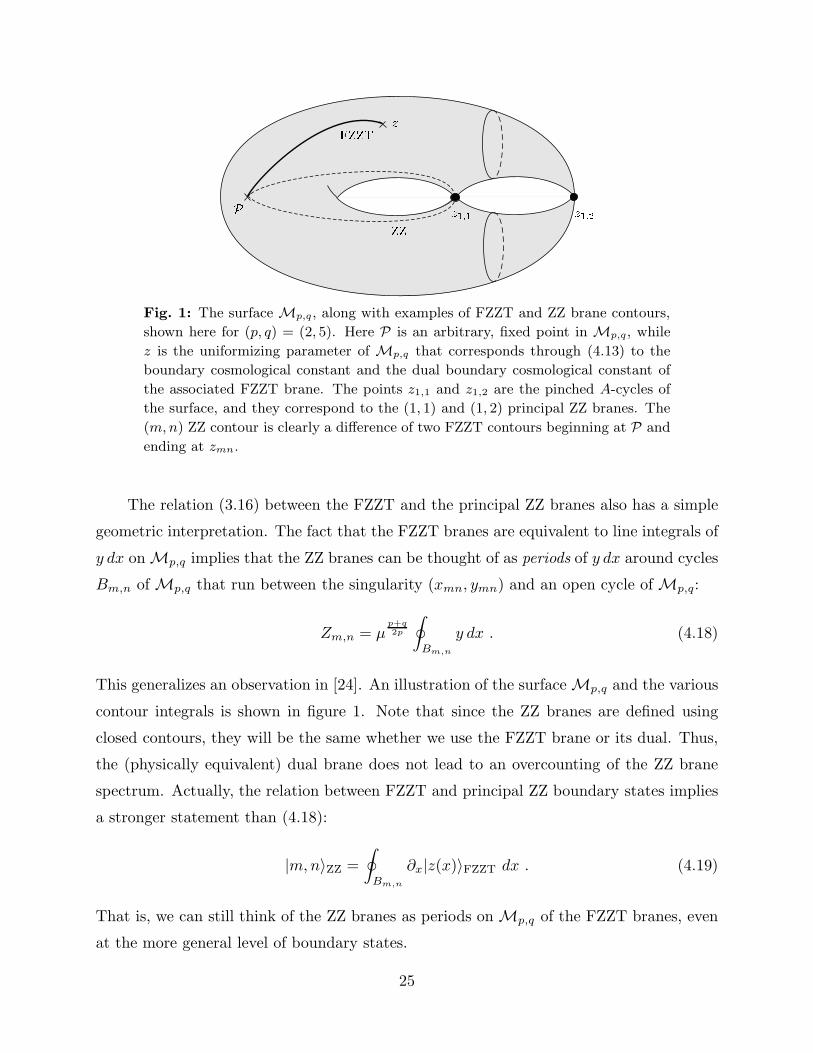
Fig. 1: The surface Mp,q, along with examples of FZZT and ZZ brane contours,

shown here for (p, q) = (2, 5). Here P is an arbitrary, fixed point in Mp,q, while

z is the uniformizing parameter of Mp,q that corresponds through (4.13) to the

boundary cosmological constant and the dual boundary cosmological constant of

the associated FZZT brane. The points z1,1 and z1,2 are the pinched A-cycles of

the surface, and they correspond to the (1, 1) and (1, 2) principal ZZ branes. The

(m, n) ZZ contour is clearly a difference of two FZZT contours beginning at P and

ending at zmn.

The relation (3.16) between the FZZT and the principal ZZ branes also has a simple

geometric interpretation. The fact that the FZZT branes are equivalent to line integrals of

y dx on Mp,q implies that the ZZ branes can be thought of as periods of y dx around cycles

Bm,n of Mp,q that run between the singularity (xmn, ymn) and an open cycle of Mp,q:

Zm,n = µp+q

2p

∮

Bm,n

y dx . (4.18)

This generalizes an observation in [24]. An illustration of the surface Mp,q and the various

contour integrals is shown in figure 1. Note that since the ZZ branes are defined using

closed contours, they will be the same whether we use the FZZT brane or its dual. Thus,

the (physically equivalent) dual brane does not lead to an overcounting of the ZZ brane

spectrum. Actually, the relation between FZZT and principal ZZ boundary states implies

a stronger statement than (4.18):

|m,n〉ZZ =

∮

Bm,n

∂x|z(x)〉FZZT dx . (4.19)

That is, we can still think of the ZZ branes as periods on Mp,q of the FZZT branes, even

at the more general level of boundary states.

25

Our geometrical interpretation implies that all of the distinct principal ZZ branes exist

and play a role in minimal string theory. We can also ask for the interpretation of the

general (t,m, n) ZZ brane (let us keep the matter state (1, 1) for simplicity). From (3.13),

the answer is clear. The (t,m, n) ZZ brane is simply (t + 1) copies of a closely related

principal ZZ brane, and therefore it corresponds to a contour integral of y dx that winds

(t+ 1) times around the B-cycle of the principal ZZ brane.

We should point out that a proposal for the interpretation of the (1, n) branes in the

c = 1 matrix model was recently advanced [53]. It would be interesting to understand its

relation to our work.

4.2. Deformations of Mp,q

So far, the discussion has been entirely in the “conformal background” where µ ≥ 0

and we have a simple world-sheet description of the theory. We have seen that in this case,

the surface Mp,q is given by a very simple curve Tq(x)− Tp(y) = 0. Here we will consider

deformations of this curve, and for simplicity we will require that they simply shift the

Np,q = (p− 1)(q − 1)/2 singularities of Mp,q:

(xi, yi) → (xi + δxi, yi + δyi) , (4.20)

without changing their total number. This leads to constraints on the form of the defor-

mations. To see what these constraints are, it is sufficient to work to linear order in the

deformation. Before the deformation, the singularities satisfy the following equations:

Tq(xi) − Tp(yi) = 0

T ′q(xi) = T ′

p(yi) = 0 .(4.21)

After the deformation, the first equation becomes

0 = Tq(xi + δxi) − Tp(yi + δyi) + δF (xi, yi)

= Tq(xi) − Tp(yi) + T ′q(xi)δxi − T ′

p(yi)δyi + δF (xi, yi) .(4.22)

Using (4.21), we see that the deformation must vanish at the singularities. This gives Np,q

constraints on the polynomial δF (x, y). The deformation of the second and third equations

of (4.21) gives no further constraints; instead, solving them yields formulas for δxi and δyi.

26

Intuitively, we expect such deformations of Mp,q to correspond in the minimal string

theory to perturbations of the background by physical vertex operators:

δS = tr,sVr,s

r = 1, . . . , p− 1, s ≤ q − 1, s 6= 0 mod q, qr − ps > 0 .(4.23)

These vertex operators exist at all ghost numbers ≤ 1 [26]. They have KPZ scaling

tr,s ∼ µp+q−qr+ps

2p (4.24)

and their Liouville momenta are given by (2.13), with the range of s extended as in (4.23).

In order to relate these perturbations to the deformations of Mp,q, notice that to

leading order in tr,s, the change in the FZZT partition function under the perturbation

(4.23) is simply the one-point function tr,s〈Vr,s〉 in the FZZT boundary state. Using (3.1),

we find that

δZ = tr,s〈Vr,s〉 = tr,sµqr−ps

2p cosh

(qr − ps

p

)πbσ . (4.25)

(The matter wavefunction will be irrelevant for this calculation, as will be other overall

normalization factors.) Since y = µ− p+q

2p ∂xZ, we find that if we hold x fixed, then y is

deformed by

δy ∼ tr,s

sinh(

qr−psp

)πbσ

sinhπbσ, (4.26)

where we have defined the dimensionless parameter tr,s = tr,sµqr−ps−p−q

2p . In terms of x

and y, the deformation of the curve is then

δr,sF (x, y) = pUp−1(y)δy ∼ tr,s

(Uq−1(x)Ts(x)Ur−1(y)−Up−1(y)Tr(y)Us−1(x)

). (4.27)

Here we have extended the definition of the Chebyshev polynomials to negative s in a

natural way: U−s−1(x) = −Us−1(x). In particular, U−1(x) = 0. Finally, using the original

curve F (x, y) = 0, we can obtain a more compact formula for the deformations of Mp,q

corresponding to the bulk physical operators (4.23):

δr,sF (x, y) = tr,s

(Uq−s−1(x)Ur−1(y) − Up−r−1(y)Us−1(x)

)

r = 1, . . . , p− 1 , s ≤ q − 1 , s 6= 0 mod q , qr − ps > 0 .

(4.28)

27

These deformations of Mp,q indeed vanish on the singularities, where Uq−1(x) = Up−1(u) =

0. Therefore, all of the perturbations of the string theory background by bulk physical

vertex operators correspond to singularity-preserving deformations of Mp,q.

It is interesting to ask whether the converse is also true, i.e. whether every possible

singularity-preserving deformation of Mp,q is given by (4.28). A careful analysis reveals

that a complete basis of such deformations is indeed given by the same formula (4.28) for

δr,sF , but with r and s taking values in a slightly larger range:

r = 1, . . . , p , s ≤ q − 1 , qr − ps > 0 . (4.29)

Thus, there are deformations of Mp,q that do not correspond to perturbations by bulk

physical vertex operators. These have r = p or s = 0 mod q. It is easy to see that the

former category can be thought of as reparametrizations of y alone:

y → y + tp,sUq−s−1(x) , s ≤ q − 1 . (4.30)

Deformations with s = 0 mod q are more complicated, but they also correspond to poly-

nomial reparametrizations of x alone.

The worldsheet interpretation of these extra deformations with r = p or s = 0 mod q

is not always clear. Recall however that the surface Mp,q originally arose from the disk

amplitude of the FZZT brane. It is reasonable then to expect the deformations associated

with such reparametrizations to be associated with open strings on the FZZT brane. For

example, Uq−1(x) is the boundary length operator as in [54]. A more detailed correspon-

dence would require a better understanding of open minimal string theory. While this is

certainly an interesting problem, it is beyond the scope of this paper.

In order to examine the relevance of the perturbations we assign weight (p, q) to (x, y)

so that F (x, y) is a quasi-homogeneous polynomial of degree pq, the degree of δr,sF (x, y)

is always q(r − 1) + p(q − s− 1). This is less than the degree of F (x, y) only for

rq − sp < p+ q . (4.31)

Such deformations of Mp,q become important at small x and y. In the string theory,

they correspond to perturbations by tachyons Tr,s with positive KPZ scaling. These are,

of course, precisely the perturbations that become increasingly relevant in the IR. This

agrees well with the intuition that flowing to the IR in the string theory corresponds to

taking x and y → 0 in Mp,q.

28

So far we have limited ourselves to deformations which do not open the singularities to

smooth A cycles. It is then natural to ask what deformations which smooth the singularities

correspond to. Given that the (m,n) ZZ brane is associated with the (m,n) singularity, it

is reasonable to expect that a background with (m,n) ZZ branes is described by a Riemann

surface with the cycle Am,n smoothed out. Since a small number of D-branes does not

affect classical string theory, we expect that the number of D-branes Nm,n needed to change

the Riemann surface to be of order 1/gs. This number can be measured by computing the

period of the one form ydx around the A cycle

∮

Am,n

ydx = gsNm,n . (4.32)

The cycle Am,n is conjugate toBm,n because they have intersection number one. Therefore,

the ZZ brane creation operator (4.19) which is an integral around Bm,n changesNm,n which

is conjugate to it by one unit. This interpretation of smoothing the (m,n) singularity is

similar to the picture which has emerged in recent studies of four dimensional gauge theories

and matrix models [55,56].

5. Minimal superstring theory

5.1. Preliminaries

We now turn to the study of minimal superstring theory. We start by reviewing the

(p, q) superminimal models. For these theories, it will be more convenient to work in α′ = 2

units. As in the bosonic theories, one must have p, q ≥ 2. Moreover, one must have either

(p, q) odd and coprime, or else (p, q) even, (p/2, q/2) coprime, and (p− q)/2 odd (the last

condition follows from modular invariance [57,24]). The superminimal models have central

charge

c = 1 − 2(p− q)2

p q(5.1)

As in the bosonic theories, primary operators Or,s are labelled by integers r and s with

r = 1, . . . , p − 1 and s = 1, . . . , q − 1 and Op−r,q−s ≡ Or,s. The crucial difference here

however is that we must distinguish between NS and the R sector operators. The NS

(R) operators have r − s even (odd). As a result, the operator dimensions are given by a

slightly more complicated expression:

∆(Or,s) = ∆(Or,s) =(rq − sp)2 − (p− q)2

8pq+

1 − (−1)r−s

32. (5.2)

29

Of particular interest is the operator O p

2 , q

2which exists only in the (p, q) even theories. It

corresponds to the supersymmetric Ramond ground state. Since it is absent in the (p, q)

odd theories, they break supersymmetry.

The operators of the (p, q) superminimal models obey fusion rules identical to those

of the bosonic models (2.3). Note that the “generators” O1,2 and O2,1 of the (p, q) super-

minimal models are in the R sector, and thus the fusion of these operators with a general

R (NS) primary results in a set of NS (R) operators.

Now consider super-Liouville theory with central charge

c = 1 + 2Q2 = 1 + 2

(b+

1

b

)2

. (5.3)

The basic vertex operators of super-Liouville are the NS operators Nα = eαφ and the R

operators R±α = σ±eαφ. These have dimensions

∆(Nα) = ∆(Nα) =1

2α(Q− α)

∆(R±α ) = ∆(R±

α ) =1

2α(Q− α) +

1

16.

(5.4)

Here σ± denotes the dimension 1/16 spin fields of the super-Liouville theory. If we study

super-Liouville as an isolated quantum field theory, only one of these fields exists following

the GSO projection, say R−α . However, if we combine it with another “matter” theory,

we sometimes need both of them before performing a GSO projection on the combined

theory.

The supersymmetric Ramond ground state has α = Q2 and hence ∆ = c

16 . It does not

correspond to two degenerate fields R± which are related by the action of the supercharge.

Instead, from solving the minisuperspace equations we find two possible wave functions

ψ+ = eµebφ

with ψ− = 0, or ψ− = e−µebφ

with ψ+ = 0 [23]. Imposing that the wave

function goes to zero as φ→ +∞, we see that depending on the sign of µ

ζ = sign(µ) , (5.5)

we have only one wave function ψ−ζ = e−|µ|ebφ

and ψζ = 0. Therefore, in pure super-

Liouville theory, where we keep only R−α= Q

2

, the Ramond ground state exists only for

positive µ. Below we will review how this conclusion changes when we add the matter

theory.

30

The degenerate primaries of super-Liouville are also similar to those of ordinary Li-

ouville. These are given by

Nαr,s= eαr,sφ , r − s ∈ 2Z

R±αr,s

= σ±eαr,sφ , r − s ∈ 2Z + 1

2αr,s =1

b(1 − r) + b(1 − s) .

(5.6)

The analogue of the bosonic fusion rules (2.9), (2.10) are for super-Liouville theory [58-61]:

R− b2Rα = [Nα− b

2] + C

(R)− (α)[Nα+ b

2]

R− b2Nα = [Rα− b

2] + C

(NS)− (α)[Rα+ b

2]

C(R)− (α) =

1

4µb2

γ(αb− b2

2)

γ(

1−b2

2

)γ(αb+ 1

2

)

C(NS)− (α) =

1

4µb2

γ(αb− b2

2 − 12 )

γ(

1−b2

2

)γ (αb)

(5.7)

with similar expressions for R− 12b

with b→ 1/b and µ→ µ, where µ is the dual cosmological

constant πµγ( Q2b ) = (πµγ( bQ

2 ))1/b2. As in the bosonic string, we will rescale µ and µ so

that they are more simply related

µ = µ1/b2 . (5.8)

We now couple the super-minimal matter theory to the super-Liouville theory to form

the minimal superstring. Imposing that the combined system has the correct central charge

fixes the Liouville parameter

b =

√p

q(5.9)

The tachyon operators Tr,s are obtained by dressing the matter operators Or,s with

Nβr,s= eβr,sφ , r − s ∈ 2Z

R±βr,s

= σ±eβr,sφ , r − s ∈ 2Z + 1

2βr,s =p+ q − rq + sp√

p q, rq − sp ≥ 0

(5.10)

and the appropriate superghosts.

The matter Ramond operators are labelled by their fermion number O±r,s. (In the

superminimal model without gravity we keep only one of them, say O+r,s.) This fermion

number should be correlated with the fermion number in super-Liouville. However, there

31

is an important subtlety which should be explained here. So far we discussed two fermion

number operators (−1)fL,M

, one in Liouville and one in the matter sector of the the-

ory. Their action on the lowest energy states in a Ramond representation is propor-

tional to iGL,M0 GL,M

0 . When we combine the Liouville and the matter states it is natural

to define left and right moving fermion numbers (−1)fL and (−1)fR such that their ac-

tion on the lowest energy states in a Ramond representation is proportional to iGL0G

M0 ,

and iGL0 G

M0 respectively. Then it is conventional to define the total fermion number as

(−1)f = (−1)fL+fR . Therefore,

(−1)f = (−1)fL+fR = (−1)fL+fM +1 , (5.11)

i.e. the total (left plus right) worldsheet fermion number differs from the sum of the fermion

numbers in the Liouville and the matter parts of the theory.

Consider now the vertex operators in the (−1/2,−1/2) ghost picture. In the 0B

theory we project on (−1)f = 1. Therefore, following (5.11) we project on (−1)fL+fM

=

−1. The candidate operators are O±r,sR

∓βr,s

(we suppress the ghosts). Only one linear

combination of them is physical [24]. The situation is more interesting when we try to

dress the supersymmetric matter groundstate (r, s) = (p2, q

2). Now there is only one matter

operator,5 say O+p

2 , q

2. Hence it should be dressed with R−

Q

2

. But as we said above, this

operator exists only for positive µ. Therefore, in the 0B minimal superstring theories with

(p, q) even, the Ramond ground state exists only for µ > 0. For (p, q) odd, there is of

course no Ramond ground state to begin with.

The situation is somewhat different in the (−1/2,−3/2) or (−3/2,−1/2) ghost picture,

where because of (5.11), we project on (−1)fL+fM

= +1. For generic (r, s) we can use

inverse picture changing to find a single vertex operator which is a linear combination of

O±r,sR

±βr,s

. The orthogonal linear combination is a gauge mode which is annihilated when

we try to picture change to the (−1/2,−1/2) picture. There are new subtleties for the

Ramond ground state (r, s) = (p2 ,

q2 ). The operator O+

p

2 , q

2R+

Q

2

exists only for negative µ.

If we try to picture change it to the (−1/2,−1/2) picture we find zero. But there could

be another operator O+p

2 , q

2R+

Q

2

, which exists only for positive µ and is related by picture

changing to the Ramond ground state O+p

2 , q

2R−

Q

2

we found in the (−1/2,−1/2) picture. The

wave function of R+Q

2

is obtained by solving the equation

(∂φ − bµebφ)ψ+ = e−µebφ

(5.12)

5 This fact is not true in other systems like the c = 1 theory.

32

subject to the boundary condition that ψ+(φ → +∞) = 0. The answer is given by an

incomplete Gamma function

ψ+ = −e−µebφ

b

∫ ∞

0

e−2t

t+ µebφdt =

{φ+ ... φ→ −∞− 1

2bµe−bφe−µebφ

(1 + ...) φ→ +∞ .(5.13)

The asymptotic form as φ → −∞ leads to the form of the operator R+Q

2

= σ+φeQ

2 φ.

Because of the factor of φ, this is not a standard Liouville operator and its analysis is

subtle. It is possible, however, to picture change it to the (−1/2,−1/2) picture, where it

is simple.

In the spacetime description of these theories, each operator is the “on-shell mode”

of a field which depends on the Liouville coordinate φ. Ramond vertex operators in the

(−1/2,−3/2) or (−3/2,−1/2) picture describe the RR scalar C, while operators in the

(−1/2,−1/2) picture describe its gradient ∂φC (more precisely, (∂φ − bµebφ)C [24]). Thus

in the spacetime description, the first candidate Ramond ground state O+p

2 , q

2R+

Q

2

, which

exists only for µ < 0 and is zero in the (−1/2,−1/2) picture, describes the constant mode

of C. It decouples from all correlation functions of local vertex operators but is important

in the coupling to D-branes. On the other hand, the second candidate operator for the

Ramond ground state O+p

2 , q

2R+

Q

2

, which exists only for µ > 0, corresponds (asymptotically

as φ → −∞) to changes of ∂φC, i.e. it describes changes in RR flux. Therefore its wave

function is linear in φ in the (−1/2,−3/2) picture, and it is constant in the (−1/2,−1/2)

picture. To summarize, in the bulk we have for µ > 0 a Ramond ground state operator

that describes changes in RR flux, but no such operator for µ < 0. But in the presence of

D-branes, there exists for µ < 0 a Ramond ground state operator that couples to D-brane

charge. In other words, for µ > 0 we can have RR flux but no charged D-branes, while the

opposite is true for µ < 0.

All of these 0B theories have a global Z2 symmetry which acts as −1 (+1) on all

R (NS) operators. We refer to this operation as (−1)FL where FL is the left-moving

spacetime fermion number. Orbifolding by this symmetry yields the 0A theories. In the

0A theories, all of the physical operators in the Ramond sector are projected out. The

only physical operators from the twisted sector are constructed out of the Ramond ground

state (r = p2, s = q

2). They exist only when such an operator could not be dressed in the

0B theory. Thus in 0A, we can have RR flux but no charged D-branes for µ < 0 and the

opposite for µ > 0.

33

Finally we should discuss the operation of (−1)fL with fL the left-moving worldsheet

fermion number. This operation is an R-transformation because it does not commute with

the supercharge. However, it is not a symmetry of the theory for two reasons. First,

the cosmological constant term in the worldsheet action explicitly breaks the would-be

symmetry: acting with (−1)fL sends µ→ −µ. The second reason this symmetry is broken

is that the transformation by (−1)fL reverses the way the GSO projection is applied in

the Ramond sector. We saw that in the 0B theory, one linear combination of the matter

operator O±r,sR

∓βr,s

was physical. After the transformation by (−1)fL , the orthogonal linear

combination will be physical. As usual, the situation is more complicated for the Ramond

ground state. The (p, q) odd models do not have a Ramond ground state; therefore the

spectrum of physical states before and after this operation are identical. Hence, we expect

that in these models, the theory with µ is dual to the theory with −µ. Moreover, at µ = 0

the operation of (−1)fL becomes a symmetry of the theory.6 On the other hand, the (p, q)

even models have a Ramond ground state, so the spectrum at µ differs from the spectrum

at −µ. An interesting special case is the pure supergravity theory (p = 2, q = 4) where

the 0B theory at µ is the same as the 0A theory at −µ [24]. For the (p, q) even models,

the transformation (−1)fL is generally not useful.

5.2. The ground ring of minimal superstring theory

As in the bosonic string, the minimal superstring theories have a ground ring consisting

of all dimension 0, ghost number 0 operators in the BRST cohomology of the theory. Since

this ground ring is nearly identical to that of the bosonic string, our discussion will be

brief. We will start with the 0B models. Just as in the bosonic string, the ground ring has

(p − 1)(q − 1) elements. The operator Or,s has Liouville momentum αr,s given by (5.6),

and it is constructed by acting on the product Or,sVαr,swith some combination of raising

operators [62-65]. Operators with r − s even (odd) are in the NS (R) sectors. We point

out that since we use the Liouville momenta αr,s of (5.6) rather than βr,s of (5.10), there

is no subtlety associated with the dressing of the Ramond ground state.

When µ = 0, Liouville momentum is conserved in the OPE, and thus one expects on

kinematical grounds that just as in the bosonic models, the ground ring is generated by

the R sector operators O1,2 and O2,1:

Or,s = Os−11,2 Or−1

2,1 (5.14)

6 A similar situation exists in the c = 1 theory where the Ramond ground state appears twice

with two different fermion numbers [23].

34

with the ring relations

Oq−11,2 = Op−1

2,1 = 0 . (5.15)

For µ 6= 0, Liouville momentum is no longer conserved, and instead one has super-Liouville

fusion rules (5.7) very similar to those of the bosonic theory. We expect the expressions

for the ring elements (5.14) and the relations (5.15) to be modified in the same way as in

the bosonic string. Once again it will be convenient to define dimensionless generators x

and y as in (2.24). Then (5.14) becomes

Or,s = µq(r−1)+p(s−1)

2p Us−1(x)Ur−1(y) , (5.16)

while the relations (5.15) become

Uq−1(x) = Up−1(y) = 0 . (5.17)

Let us now discuss the relations in the tachyon module. As in the bosonic theory we

have

Tr,s = µ1−sOr,sT1,1 = µq(r−1)−p(s−1)

2p Us−1

(x)Ur−1

(y)T1,1 . (5.18)

The Ramond ground state in the even (p, q) models leads to a new complication. As

we have seen, the tachyon T p

2 , q

2exists in the 0B theory only for positive µ. (For the

discussion of correlation functions of physical vertex operators without D-branes we can

neglect the similar operator in the (−1/2,−3/2) ghost picture which exists only for negative

µ.) Therefore, for positive µ we have tachyons with rq − sp ≥ 0, while for negative µ we

have only the tachyons with rq − sp > 0. This truncation can be achieved by imposing

Tp−r,q−s = ζµps−qr

p Tr,s . (5.19)

As in the bosonic string, it is enough to require that

(Uq−2(x) − ζUp−2(y))T1,1 = 0 . (5.20)

This will guarantee all of the relations (5.19).

The discussion of the ground ring and the tachyon module has so far been entirely for

the 0B models. The ground ring for 0A follows trivially from that of the 0B: since we need

not worry about the Ramond ground state, we simply project out the R sector of the 0B

ground ring to obtain the ground ring of 0A. Thus the ground ring of 0A is generated by

the NS operators O1,3, O2,2 and O3,1.

It is straightforward to extend the calculation of tachyon correlation functions in the

bosonic string (section 2.2) to the superstring. Since the results are nearly identical to the

bosonic string, we will not discuss them here.

35

6. FZZT and ZZ branes of minimal superstring theory

6.1. Boundary states

Here we will extend the discussion of the FZZT and the ZZ branes of the previous

sections to the (p, q) superminimal models coupled to gravity. The analysis will become

more complicated, owing to the presence of the NS and R sectors, the two different GSO

projections, and the option of having negative µ. Nevertheless, we will find that the

supersymmetric and bosonic theories share many features in common.

As in the bosonic string, the boundary states are labelled by a Liouville parameter σ

and matter labels (k, l). In addition to these labels there are also a supercharge parameter

η related to the linear combination of left and right moving supercharges Gr + iηG−r

which annihilate the state, and the R-R “charge” ξ = ±1. Finally, the boundary states

also depend on ζ = sign(µ).

Consider first the branes in the positive µ (ζ = +1) theory. In the expressions that

follow, it will be implicit that the matter representation (k, l) and the parameter η are

correlated by the condition

(−1)k+l = η . (6.1)

This follows from the boundary conditions on the supercharge, which imply that the Cardy

states with η = 1 (η = −1) in are in the NS (R) sector. Using the results of [60,61], we

write the boundary states as:

|σ, (k, l); ξ, η = +1〉∣∣ζ=+1

=

∫ ∞

0

dP

(cos(πPσ)ANS(P )|P, (k, l); η = +1〉〉NS

+ξ cos(πPσ)AR(P )|P, (k, l); η = +1〉〉R)

|σ, (k, l); ξ, η = −1〉∣∣ζ=+1

=

∫ ∞

0

dP

(cos(πPσ)ANS(P )|P, (k, l); η = −1〉〉NS

−iξ sin(πPσ)AR(P )|P, (k, l); η = −1〉〉R),

(6.2)

where the Liouville wavefunctions are given by

ANS(P ) =

( |µ|4

)iP/b Γ(1 − iP b)Γ(1 − iPb

)√2πP

AR(P ) =

( |µ|4

)iP/b1

πb2Γ

(1

2− iP b

)Γ

(1

2− iP

b

),

(6.3)

36

and the boundary cosmological constant depends on the various parameters as

µB√|µ|

=

{ξ cosh(πbσ

2 ) η = +1

ξ sinh(πbσ2 ) η = −1 .

(6.4)

The factor of ξ in the definition of µB was included for convenience, so as to make explicit

the (−1)FL symmetry of the theory. The action of (−1)FL maps ξ → −ξ since it acts as

−1 (+1) on all R (NS) states. It also maps µB → −µB , since µB is the coefficient of a

boundary fermion which transforms like a bulk spin field.

The states |P, (k, l); η〉〉NS,R appearing on the RHS of (6.2) are shorthand for the

following linear combination the matter (M), Liouville (L) and superghost (G) Ishibashi

states (i.e. strictly, they are not Ishibashi states):

|P, (k, l); η〉〉NS =∑

k′+l′ even

ψ(η,ζ=+1)(k, l; k′, l′)|NS; (k′, l′); η〉〉M |NS;P ; η〉〉L|NS; η〉〉G

|P, (k, l); η〉〉R =∑

k′+l′ odd

ψ(η,ζ=+1)(k, l; k′, l′)|R; (k′, l′); η〉〉M |R;P ; η〉〉L|R; η〉〉G .

(6.5)

A few comments are in order.

1. For the superghost states it is convenient to work in the (−1,−1) picture in the NS

sector and in the (−1/2,−3/2) or (−3/2,−1/2) in the R sector. In these pictures we

see the elementary spacetime fields and the inner products of the states are simplest.

2. The individual Ishibashi states in each sum must have the same label η = ±1. This

guarantees that the linear combinations Gr + iηG−r annihilate the state, where G and

G are the total left and right-moving supercharges of the system. Actually, this would

have allowed also a linear combination of Liouville and matter states with opposite η.

Such a linear combination is incompatible with the P dependence in the Cardy state,

which is different for the two signs of η.

3. The restriction in the sums to k′ + l′ even or k′ + l′ odd guarantees that we include

only NS or R matter Ishibashi states. The “matter wavefunctions” ψ(η,ζ)(k, l; k′, l′)

are closely related to the modular S-matrix elements of the combined superminimal

model and super-Liouville. Although they can be computed, we will not do that here.

4. It is important to note that the Cardy states (6.2) are not just products of Cardy

states of the matter, Liouville and ghost sectors, as they were in the bosonic string.

This is because our system is not simply the product of the superminimal model and

37

super-Liouville theory. Instead, the NS sector is constructed out of the NS sectors

of the two theories by projecting on (−1)f = 1, where f = fL + fR is the total

worldsheet fermion number operator in the combined theory. Similarly, the R sector

is made out of the R sectors of the two theories, again by projecting on fixed (−1)f .

In the (−1/2,−3/2) or (−3/2,−1/2) picture its value is −1 in the 0B theory and +1

in the 0A theory.

Let us discuss in some detail the construction of the individual Ishibashi states

|NS, h, η〉〉L,M and |R, h, η〉〉L,M in (6.5), where here we will use h to denote the con-

formal weight of the associated Liouville or matter primary instead of the labels P and

(k, l). In the NS sector, the Ishibashi states are linear combinations of NS states of fixed

(−1)fL

|NS, h, η〉〉L,M =(1 + η f(h, c)GL,M

−1/2GL,M−1/2 + . . .

)|NS, h〉L,M , (6.6)

where f(h, c) is η-independent and is fixed by the supersymmetry constraints, and

|NS, h〉L,M denotes the associated primary state. Note that this expression is analogous

to the fact that in the Ising model one uses the Ishibashi states |1〉〉 + η|ψ〉〉 in forming

Cardy states.

In the R sector, every generic (i.e. nonsupersymmetric) representation leads to two

Ishibashi states which are annihilated by Gr + iηG−r for η = ±1. Consider first the matter

or the Liouville part of the theory independently. Then the Ishibashi state in each of them

is

|R, h, η〉〉L,M =(1 + a(h, c)LL,M

−1 LL,M−1 + η b(h, c)GL,M

−1 GL,M−1

)|R, h, η〉L,M

+(c(h, c)GL,M

−1 LL,M−1 + η d(h, c)LL,M

−1 GL,M−1

)|R, h,−η〉L,M + . . .

(6.7)

where again the coefficients appearing here are η-independent and are determined by the

supersymmetry constraints. These Ishibashi states are eigenstates of the fermion number

operator in each sector (−1)fL,M

(−1)fL,M |R, h, η〉〉L,M = −η|R, h, η〉〉L,M . (6.8)

Using (5.11) we conclude that

(−1)f |R, h, η〉〉L|R, h′, η〉〉M = −|R, h, η〉〉L|R, h′, η〉〉M (6.9)

38

with generic values of h and h′. Therefore, in the 0B theory all the terms in the right hand

side of (6.5) made out of these representations satisfy the GSO projection, while no such

state survives the projection in the 0A theory.

The situation is somewhat different for the matter R ground state, which exists in

the even (p, q) superminimal models and has conformal weight h0 = cM

16 . The matter R

ground state must have (−1)fM

= 1, but it still leads to two Ishibashi states with η = ±1

and (−1)fM

= 1. These take the form

|R, h0, η〉〉M =(1 + a(h0, c)L

M−1L

M−1 + η b(h0, c)G

M−1G

M−1 + . . .

)|R, h0〉M , (6.10)

where the coefficients are the same as in (6.7). (One can also show that c(h0, c) = d(h0, c) =

0.) Meanwhile, the Liouville Ishibashi state still has (−1)fL

= −η, and therefore the

contribution of the matter R ground state to (6.5) is restricted by

ψ(η=+1,ζ=+1)(k, l;p

2,q

2) = 0 (0B)

ψ(η=−1,ζ=+1)(k, l;p

2,q

2) = 0 (0A) .

(6.11)

Now let us examine the situation for negative µ (ζ = −1). We start by ignoring the

matter and the ghosts. The sign of µ can be changed in the super-Liouville part of the

theory by acting with the Z2 R-transformation (−1)fL . This is not a symmetry of the

theory, as it changes the parameter µ. Also, this transformation changes the sign of the

projection in the Ramond sector. As for the boundary states, this transformation has the

effect of reversing the sign of η, since it sends G → −G without changing G. Therefore,

the boundary super-Liouville theory depends only on η = ηζ.

Adding back in the matter and superghost sectors, we see that if we want to perform

such an R-transformation on the Liouville sector of the theory, we should do it in all

the sectors because the total supercharge G is gauged. This is complicated when the

matter theory does not have such an R-symmetry. Nevertheless, we can perform such a

transformation and label the states by their value of η. Then our expression (6.2) for the

boundary states becomes

|σ, (k, l); ξ, η = +1, ζ〉 =

∫ ∞

0

dP

(cos(πPσ)ANS(P )|P, (k, l); η = +1, ζ〉〉NS

+ ξ cos(πPσ)AR(P )|P, (k, l); η = +1, ζ〉〉R)

|σ, (k, l); ξ, η = −1, ζ〉 =

∫ ∞

0

dP

(cos(πPσ)ANS(P )|P, (k, l); η = −1, ζ〉〉NS

− iξ sin(πPσ)AR(P )|P, (k, l); η = −1, ζ〉〉R),

(6.12)

39

where the Liouville wavefunctions are again given by (6.3) and the expression for the

boundary cosmological constant (6.4) is generalized to

µB√|µ|

=

{ξ cosh(πbσ

2 ) η = +1

ξ sinh(πbσ2 ) η = −1 .

(6.13)

Now the Cardy states with η = 1 (η = −1) in (6.12) are in the NS (R) sector, and therefore

their matter representation (k, l) should satisfy

(−1)k+l = η . (6.14)

The Ishibashi states (6.5) are generalized to

|P, (k, l); η, ζ〉〉NS =∑

k′+l′ even

ψ(η,ζ)

(k, l; k′, l′)|NS; (k′, l′); η〉〉M |NS;P ; η〉〉L|NS; η〉〉G

|P, (k, l); η, ζ〉〉R =∑

k′+l′ odd

ψ(η,ζ)

(k, l; k′, l′)|R; (k′, l′); η〉〉M |R;P ; η〉〉L|R; η〉〉G .

(6.15)

Here the only dependence on ζ for fixed η is through the “matter wavefunctions”

ψ(η,ζ)

(k, l; k′, l′). This is important in the even (p, q) models which include the Ramond

ground state. Here the GSO condition implies

ψ(η=+ζ,ζ)

(k, l;p

2,q

2) = 0 (0B)

ψ(η=−ζ,ζ)

(k, l;p

2,q

2) = 0 (0A) .

(6.16)

That is, the Ramond ground state does not contribute to the sum over Ishibashi states for

the η = +1 (−1) brane in the 0B (0A) theory.

To illustrate the general discussion above, let us consider the simplest example of pure

supergravity (p, q) = (2, 4), which does not have matter at all. (Alternatively, the matter

includes the identity and the R-ground state.) Imposing the 0B GSO condition,7 (6.12)

becomes

|σ; ξ, η = +1, ζ = +1〉 =

∫ ∞

0

dP cos(πPσ)ANS(P )|NS;P ; η〉〉L|NS; η〉〉G

|σ; ξ, η = −1, ζ = +1〉 =

∫ ∞

0

dP

(cos(πPσ)ANS(P )|NS;P ; η〉〉L|NS; η〉〉G

− iξ sin(πPσ)AR(P )|R;P ; η〉〉L|R; η〉〉G)

(6.17)

7 If instead we use the 0A GSO projection, the results below are the same with ζ → −ζ and

η → −η [24].

40

for µ positive. In this phase, the vertex operator for the zero mode of C does not exist,

and therefore neither brane is charged. Now consider µ negative. We have

|σ; ξ, η = +1, ζ = −1〉 =

∫ ∞

0

dP cos(πPσ)ANS(P )|NS;P ; η〉〉L|NS; η〉〉G

|σ; ξ, η = −1, ζ = −1〉 =

∫ ∞

0

dP

(cos(πPσ)ANS(P )|NS;P ; η〉〉L|NS; η〉〉G

+ ξ cos(πPσ)AR(P )|R;P ; η〉〉L|R; η〉〉G).

(6.18)

In this phase, the η = +1 brane is again uncharged, but now the η = −1 brane carries

charge. This agrees with the discussion below (5.13), where we saw that for µ < 0 we can

have charged branes but not flux.

6.2. FZZT one-point functions and the role of ξ

Let us use the expression (6.12) for the FZZT boundary state to study the one-point

functions of physical operators on the disk with FZZT-type boundary conditions. We

expect to find similar results as in the bosonic string, where not all FZZT states are

distinct in the BRST cohomology. In particular, we expect (see (3.8)) that all of the FZZT

branes with arbitrary matter label can be reduced to elementary branes with fixed matter

label, say (1, 1) for NS branes and (1, 2) or (2, 1) for R branes. To actually prove this at the

level of the one-point functions as we did for the bosonic string would require knowledge

of the matter wavefunctions, which we do not presently have. Thus we will simply assume

that it can be done, and from this point onwards we will suppress the matter label and

refer to the FZZT branes as | σ; ξ, η, ζ〉.Now consider the FZZT one-point functions of the tachyon operators Tr,s. From (6.12)

we find the (σ, ξ)-dependent part of these one-point functions can be expressed compactly

with the following:

〈Tr,s| σ; ξ, η, ζ〉 ∝ ξr+s cosh

(π(rq − sp)σ

2√pq

+iπ(r + s)ν

2

)(6.19)

where we have defined

ν =1 − η

2=

{0 for η = +11 for η = −1

(6.20)

The one-point functions of the other physical operators are also given by (6.19), but with

different values of s. Thus physical one-point functions are invariant under the transfor-

mations

(σ, ξ) → (−σ, η ξ), (σ ± 2i√pq, (−1)pξ) (6.21)

41

Note that the first transformation is true at the level of the boundary state (6.12). The

second transformation is only true for physical one-point functions, which is evidence

that FZZT states related by this transformation differ by a BRST exact state. These

transformations suggest that we define

z =

cosh

(πσ

2√

pq− iπν

2

)(p, q) odd

cosh(

πσ√pq − iπν

2

)(p, q) even

(6.22)

and label the FZZT brane by z:

| σ; ξ, η, ζ〉 → | z; ξ, η, ζ〉 (6.23)

so that at fixed ξ, two FZZT branes labelled by z and z′ are equal if and only if z = z′.

The parametrization in terms of z eliminates some, but not all of the redundancy

of description implied by the transformations (6.21). The remaining redundancy involves

changing the sign of ξ. Indeed, we see that when η = −1 or (p, q) is odd, a state with

(z,−ξ) is equivalent to a state with (−z, ξ). For these states, ξ is a redundant label which

can be removed by analytic continuation in z. The only states for which ξ cannot be

eliminated in this way are those with η = +1 when (p, q) is even.8 In section 7, we will

see how these disparate facts can be all understood geometrically and in a unified way, in

terms of an auxiliary Riemann surface.

Finally, we note that when (p, q) is odd, the transformation

(σ, η) → (i√pq − σ, −η) (6.24)

leaves the σ-dependent part of the one-point functions (6.19) unchanged. Moreover, the

transformation also leaves z unchanged. This suggests that when (p, q) is odd, the FZZT

states with η = −1 are equivalent to the FZZT states with η = +1 (but with different σ)

in the BRST cohomology. Let us assume that this is true, and focus our attention only

on the states with η = +1 when (p, q) is odd. We will also motivate this simplification

geometrically in section 7 and we will use it in section 8.

8 We could further reparametrize the FZZT branes so as to remove the redundancy by ξ.

However, as this would needlessly complicate the notation, we prefer to continue labelling the

FZZT branes with ξ, even in the cases where it is unnecessary.

42

6.3. ZZ branes and their one-point functions

The discussion of the ZZ boundary states is analogous to that of the FZZT states, so

we will simply write down the relevant expressions. Here we will not attempt to analyze

the subtleties of the degenerate super-Virasoro representations that arise at rational b2.

For the bosonic string, we found that these subtleties only pertained to (m,n) ZZ branes

with m > p or n > q. The ZZ boundary states with m ≤ p and n ≤ q were given by

the formula for generic b, and could be written as a difference of just two FZZT branes.

Therefore the subtleties at rational b2 did not affect our final conclusion in the bosonic

string, which was that the set of all (m,n) ZZ branes could be reduced to a principal

set with m < p and n < q and mq − np > 0. As we expect a similar conclusion in the

superstring, let us restrict our attention from the outset to ZZ boundary states with m ≤ p

and n ≤ q. Then by analogy with the bosonic string, these should be given by the formula

at generic b [60,61]:

|(m,n), (k, l); ξ, η = +1, ζ〉 =

2

∫ ∞

0

dP

(sinh

(πP mb

)sinh

(πP b n

)ANS(P )|P, (k, l); η, ζ〉〉NS

+ ξ sinh(πmP

b+iπn

2

)sinh

(πnP b− iπn

2

)AR(P )|P, (k, l); η, ζ〉〉R

)

|(m,n), (k, l); ξ, η = −1, ζ〉 =

2

∫ ∞

0

dP

(sinh

(πP mb

)sinh

(πP b n

)ANS(P )|P, (k, l); η, ζ〉〉NS

+ ξ cosh(πmP

b+iπn

2

)sinh

(πnP b− iπn

2

)AR(P )|P, (k, l); η, ζ〉〉R

).

(6.25)

As for the FZZT branes, the parameter η determines whether the Cardy state is NS or R.

Thus we must require

(−1)m+n = (−1)k+l = η . (6.26)

Also, we will assume as we did for the FZZT branes that the ZZ branes with different

matter labels can be reduced down to ZZ branes with fixed matter label.

Expanding the products of cosh and sinh using standard trigonometric identities and

comparing with (6.12), we see that the ZZ branes with m ≤ p and n ≤ q can be written

in terms of the FZZT branes as (we suppress the labels (η, ζ)):

|m,n; ξ〉 = | z = z(m,n); ξ〉 − | z = z(m,−n); (−1)nξ〉 (6.27)

43

where z(m,n) ≡ z(σ(m,n)) was defined in (6.22), and

σ(m,n) = i(mb

+ nb). (6.28)

The boundary cosmological constant corresponding to σ(m,n) is

µB(m,n, ξ) = µB(m,−n, (−1)nξ) =

{ξ√|µ| cos π

2 (m+ nb2) η = +1

i ξ√|µ| sin π

2(m+ nb2) η = −1 .

(6.29)

Note that the two FZZT branes in the right hand side of (6.27) always have the same value

of µB .

As in the bosonic string, we do not expect all of the ZZ branes to be distinct in the full

string theory; rather, we expect many to differ by BRST null states. Indeed, the formula

(6.27) for the ZZ branes immediately implies the identification

|p−m, q − n; (−1)q+m+nξ〉 = |m,n; ξ〉 (6.30)

modulo BRST null states. Moreover, a straightforward computation using (6.25) shows

that the one-point functions of physical operators all vanish when m = p or n = q. This

suggests that in the BRST cohomology:

|m,n; ξ〉 = 0, when m = p or n = q . (6.31)

In the next section, we will also motivate these identifications from a more geometrical

point of view, as was done for the bosonic string.

Using the identifications (6.30) and (6.31), we can reduce the infinite set of (m,n, ξ)

ZZ branes down to what we will call, as in the bosonic string, the principal ZZ branes.

Let us define B = {(m,n)| m = 1, . . . , p − 1, n = 1, . . . , q − 1}. Then for (p, q) even, the

principal ZZ branes are

η = +1 : (m,n, ξ) , (m,n) ∈ B , m+ n even , mq − np ≥ 0 , ξ = ±1

η = −1 : (m,n, ξ) , (m,n) ∈ B , m+ n odd , ξ = +1 ,(6.32)

giving a total of (p−1)(q−1)±12 principal ZZ branes for η = ±1. On the other hand, for (p, q)

odd, the principal ZZ branes are

(m,n, ξ) , (m,n) ∈ B , m+ n even , ξ = +1 (and η = +1) (6.33)

44

giving a total of (p−1)(q−1)2 principal ZZ branes for (p, q) odd. Notice that we have restricted

ourselves to the ZZ branes with η = +1. Since the map (6.24) (σ, η) → (i√pq − σ, −η)

leaves z unchanged, it preserves the formula (6.27) and maps ZZ branes with η to ZZ

branes with −η.In the bosonic string, we saw that we could normalize the ground ring elements so

that the principal ZZ branes became eigenstates of the ground ring. We expect similar

phenomena to occur in the superstring. To make more precise statements, we would need

to have explicit formulas for the matter wavefunctions. We will leave this for future work.

7. Geometric interpretation of minimal superstring theory

7.1. The surfaces M±p,q and their analytic structure

As in the bosonic string, we can understand many of the features of the boundary

states using an auxiliary Riemann surface that emerges from the FZZT partition function.

We start as before with the disk one-point function of the cosmological constant operator.

This is given by:

∂µZ∣∣µB

= 〈ψψebφ〉 = A(b)(√|µ|)1/b2−1 cosh

(b− 1

b

)πσ

2. (7.1)

Notice the similarity to the bosonic one-point function (4.2). The difference comes in the

relation between σ and µB for η = −1. For simplicity, we will limit our discussion in the

superstring to the FZZT brane and not its dual. The relationship between the FZZT brane

and its dual is exactly analogous to that in the bosonic string.

Integrating (7.1) leads to

Z = C(b)(√|µ|)1/b2+1 ×

{b2 cosh

(πσ2b

)cosh

(πbσ2

)− sinh

(πσ2b

)sinh

(πbσ2

)η = +1

b2 sinh(

πσ2b

)sinh

(πbσ2

)− cosh

(πσ2b

)cosh

(πbσ2

)η = −1 ,

(7.2)

and differentiating this with respect to µB , we find

∂µBZ∣∣µ

=

{(√

|µ|)1/b2ξ cosh(

πσ2b

)η = +1

(√

|µ|)1/b2ξ sinh(

πσ2b

)η = −1 .

(7.3)

In (7.1) and (7.2) above, A(b) and C(b) are overall normalization factors that were chosen

so as to make the normalization of (7.3) unity. As in the bosonic string, we suppress the

contribution of the matter sector, since this is µ and µB independent. The two types of

45

FZZT brane lead to two Riemann surfaces; we will call them Mηp,q. For reasons that will

shortly become clear, we will parametrize these surfaces with slightly different dimension-

less coordinates:

M+p,q : x =

µB√µ, y =

∂µBZ√µ

,

M−p,q : x =

iµB√µ, y =

i∂µBZ√µ

.

(7.4)

Then in terms of x and y, the surfaces are described by the polynomial equations:

0 = F (x, y) =

{Tq(x) − Tp(y) η = +1

(−1)p−q

2 Tq(x) − Tp(y) η = −1 .(7.5)

Note that we have assumed in writing (7.5) that (p, q) are either both odd or both even;

otherwise there could be additional phases arising from the factor of ξ in the definition of

the coordinates. It is interesting that for (p, q) odd, the phase in front of Tq in the second

line of (7.5) can be absorbed into the argument of the Chebyshev polynomial. Thus, for

(p, q) odd the surfaces M+p,q and M−

p,q are identical, and we will limit our discussion to

M+p,q without loss of generality. However, for (p, q) even, since (p− q)/2 is odd the phase

cannot be absorbed, and therefore these surfaces are different. This is consistent with the

suggestion that for (p, q) odd, boundary states with η = ±1 become equivalent, while for

(p, q) even, η labels distinct states.

As in the bosonic string, a natural uniformization of these surfaces is provided by the

parameter z defined in (6.22). The coordinates of Mηp,q are given in terms of z by

(x, y) =

(ξTp(z), ξTq(z)

)(p, q) odd

(ξT p

2(z), ξT q

2(z))

(p, q) even and η = +1(ξzU p

2−1(√

1 − z2), ξzU q

2−1(√

1 − z2))

(p, q) even and η = −1

(7.6)

Therefore, for fixed ξ, z ∈ C covers Mηp,q exactly once, except for when (p, q) is even and

η = −1, where we must extend z to a two-sheeted cover of the complex plane in order to

cover the surface once. Notice also that ξ can be absorbed into the definition of z except

when (p, q) is even and η = +1. (Recall that for the (p, q) even models, either p/2 or q/2

must be even.) This gives a nice geometric interpretation to the results of section 6, where

we saw that only for (p, q) even and η = 1 did the parameter ξ label two distinct FZZT

boundary states. The fact that ξ cannot be eliminated in this case also has implications

for the analytic structure of the associated surface that we will discuss below.

46

It is straightforward to work out the analytic structure of M+p,q and M−

p,q. One can

use either the condition F = dF = 0, or equivalently one can look for points (x, y) that

correspond to multiple values of z. Either way, we must consider the following three cases:

1. (p, q) odd and coprime (η = +1)

For (p, q) odd, M+p,q is identical to the bosonic surface Mp,q (figure 1). Thus it has

the (p− 1)(q − 1)/2 singularities given by (4.14), which we include here for the sake

of completeness:

(x, y) =

(cos

π(jq + kp)

q, cos

π(jq + kp)

p

),

1 ≤ j ≤ p− 1, 1 ≤ k ≤ q − 1, j q − k p > 0

(7.7)

2. (p, q) even, (p2 ,

q2 ) coprime, p−q

2 odd, η = +1

For (p, q) even, the surface M+p,q is actually quite special. Since its curve can be

written as T q

2(x)2 = T p

2(y)2, the surface splits into two separate branches described

by T q

2(x) = ±T p

2(y), with each branch itself a Riemann surface. We will denote these

surfaces by(M+

p,q

)±. Note that since either p

2or q

2must be odd, the two branches

of the surface are related by the map (x, y) → (−x,−y). From the definition (7.4) of

x and y, we see that this is just the action of ξ → −ξ. Thus we can think of the two

branches as(M+

p,q

)ξ. We will elaborate on this identification of the branches with ξ

shortly.

One can easily check that M+p,q has (p−1)(q−1)+1

2singularities described by

(x, y) =

(cos

jπ

q, cos

kπ

p

), j = 1, . . . , q − 1, k = 1 . . . , p− 1, k − j = 0 mod2.

(7.8)

There are two types of singularity: those that are singularities of(M+

p,q

)ξ

individually,

which we will call regular singularities; and those that join the two branches, which

we will call connecting singularities. The distinction between the two is quite simple

algebraically: connecting singularities satisfy T q

2(x) = T p

2(y) = 0, while the regular

singularities have T q

2(x) and T p

2(y) 6= 0. Counting the number of singularities of

each type is also easy. There are p q4

connecting singularities; and (p−2)(q−2)8

regular

singularities on each branch of M+p,q. An example of this kind of surface is shown in

figure 2.

47

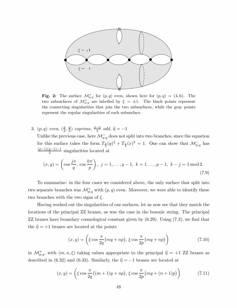
Fig. 2: The surface M+p,q for (p, q) even, shown here for (p, q) = (4, 6). The

two subsurfaces of M+p,q are labelled by ξ = ±1. The black points represent

the connecting singularities that join the two subsurfaces, while the gray points

represent the regular singularities of each subsurface.

3. (p, q) even, (p2 ,

q2 ) coprime, p−q

2 odd, η = −1

Unlike the previous case, here M−p,q does not split into two branches, since the equation

for this surface takes the form T p

2(y)2 + T q

2(x)2 = 1. One can show that M−

p,q has(p−1)(q−1)−1

2 singularities located at

(x, y) =

(cos

jπ

q, cos

kπ

p

), j = 1, . . . , q − 1, k = 1 . . . , p− 1, k − j = 1 mod2.

(7.9)

To summarize: in the four cases we considered above, the only surface that split into

two separate branches was M+p,q with (p, q) even. Moreover, we were able to identify these

two branches with the two signs of ξ.

Having worked out the singularities of our surfaces, let us now see that they match the

locations of the principal ZZ branes, as was the case in the bosonic string. The principal

ZZ branes have boundary cosmological constant given by (6.29). Using (7.3), we find that

the η = +1 branes are located at the points

(x, y) =

(ξ cos

π

2q

(mq + np

), ξ cos

π

2p

(mq + np

))(7.10)

in M+p,q, with (m,n, ξ) taking values appropriate to the principal η = +1 ZZ branes as

described in (6.32) and (6.33). Similarly, the η = −1 branes are located at

(x, y) =

(ξ cos

π

2q

((m+ 1)q + np

), ξ cos

π

2p

(mq + (n+ 1)p

))(7.11)

48

in M−p,q, with (m,n, ξ) again taking the appropriate values. We claim that the locations

of the principal ZZ branes are just a different parametrization of the singularities of M±p,q.

Let us briefly sketch a proof. First, one can show that they indeed lie at the singularities

by checking that their locations (x, y) satisfy the conditions F (x, y) = 0 and dF (x, y) = 0.

Since the locations of the principal ZZ branes are all distinct, and there are exactly as many

principal η ZZ branes as there are singularities of Mηp,q, it follows that their locations match

the singularities exactly.

Combining the calculations of the one-point functions in the previous section with the

geometric results here, we can summarize our conclusions regarding the ZZ branes very

succintly. These conclusions are essentially the same as in the bosonic string. The η = ±1

principal ZZ branes are located at the singularities of our surfaces M±p,q. ZZ branes located

at the same singularity of the surface differ by BRST null states, while ZZ branes located

at different singularities are distinct BRST cohomology classes. Finally, ZZ branes that

are not located at singularities of the surface are themselves BRST null.

By analogy with the bosonic string, we also expect that the η FZZT and ZZ branes

can be represented as contour integrals of a one-form (or boundary state) on the surfaces

Mηp,q. For instance, in the cases where ξ is a redundant parameter, the η FZZT branes

are given by line integrals of the one-form y dx on Mηp,q:

Z(µB) = µp+q

2p

∫ x(µB)

Py dx , (7.12)

where P is an arbitrary fixed point in Mηp,q. For the case of (p, q) even and η = +1 where ξ

actually labels two distinct branes, we saw above that the corresponding surface splits into

two separate branches. These branches were also labelled by ξ, and they were connected

by singularities. Thus in this case alone can we define two inequivalent line integrals on

the surface; these clearly correspond to the two types of FZZT brane:

Z(µB , ξ) = µp+q

2p

∫ x(µB)

Pξ

y dx . (7.13)

Here Pξ ∈(M+

p,q

)ξ

is an arbitrary fixed point on the branch labelled by ξ.

We can consider the ZZ branes in a similar way. When ξ is a redundant parameter,

the relation (6.27) between the ZZ and FZZT branes, together with (7.12), implies that

49

the ZZ branes can be written as closed contour integrals of y dx. As in the bosonic string,

we can promote this to a relation between boundary states:

|m,n; η〉 =

∮

Bm,n

∂x|z(x); η〉 dx , (7.14)

where the contour Bm,n runs through the open cycle on M±p,q and the singularity associated

to the (m,n) ZZ brane. For η = +1 and (p, q) odd, we saw that ξ was only redundant

modulo BRST exact states. Thus in this case, we must interpret (7.14) as a relation in

the BRST cohomology of the full theory.

Once again, the case of (p, q) even and η = +1 has more structure. The relation (6.27)

implies that for n even, the ZZ branes are differences of FZZT branes of the same ξ. Using

(7.13), we see that for n even, we can write the ZZ brane as a closed contour of the FZZT

brane:

|m,n; ξ, η = 1〉∣∣(m,n) even

=

∮

Bξm,n

∂x|z(x); ξ, η = 1〉 dx , (7.15)

where the contour Bξm,n runs through the open cycle on

(M+

p,q

)ξ

and the singularity

associated to the (m,n, ξ) ZZ brane. On the other hand, for n odd, the relation (6.27) says

that the ZZ branes are differences of FZZT branes of opposite ξ. Thus these ZZ branes

are not described by closed contours, but rather by line integrals from one branch of M+p,q

to another:

|m,n; ξ, η = 1〉∣∣(m,n) odd

=

∫ xm,n

Pξ

∂x|z(x), ξ, η = 1〉 dx−∫ xm,n

P−ξ

∂x|z(x),−ξ, η = 1〉 dx .

(7.16)

Note that in order for these relations to be true, the properties of the singularity associated

to the (m,n, ξ) ZZ brane must depend on n in a very non-trivial way: for n even, the

singularity must be a regular singularity of the branch(M+

p,q

)ξ, while for n odd, it must

be a connecting singularity between the two branches. (See the discussion following (7.8)

for a description of the two types of singularities.) Substituting the locations of the ZZ

branes into T q

2(x) and T p

2(y), we immediately find that these polynomials are zero for the

n odd branes and nonzero for the n even branes. Therefore the n odd (even) branes are

indeed located at the connecting (regular) singularities, which is a highly non-trivial check

of our relations (7.15) and (7.16). Figure 3 illustrates the different types of FZZT and ZZ

branes for this surface.

50

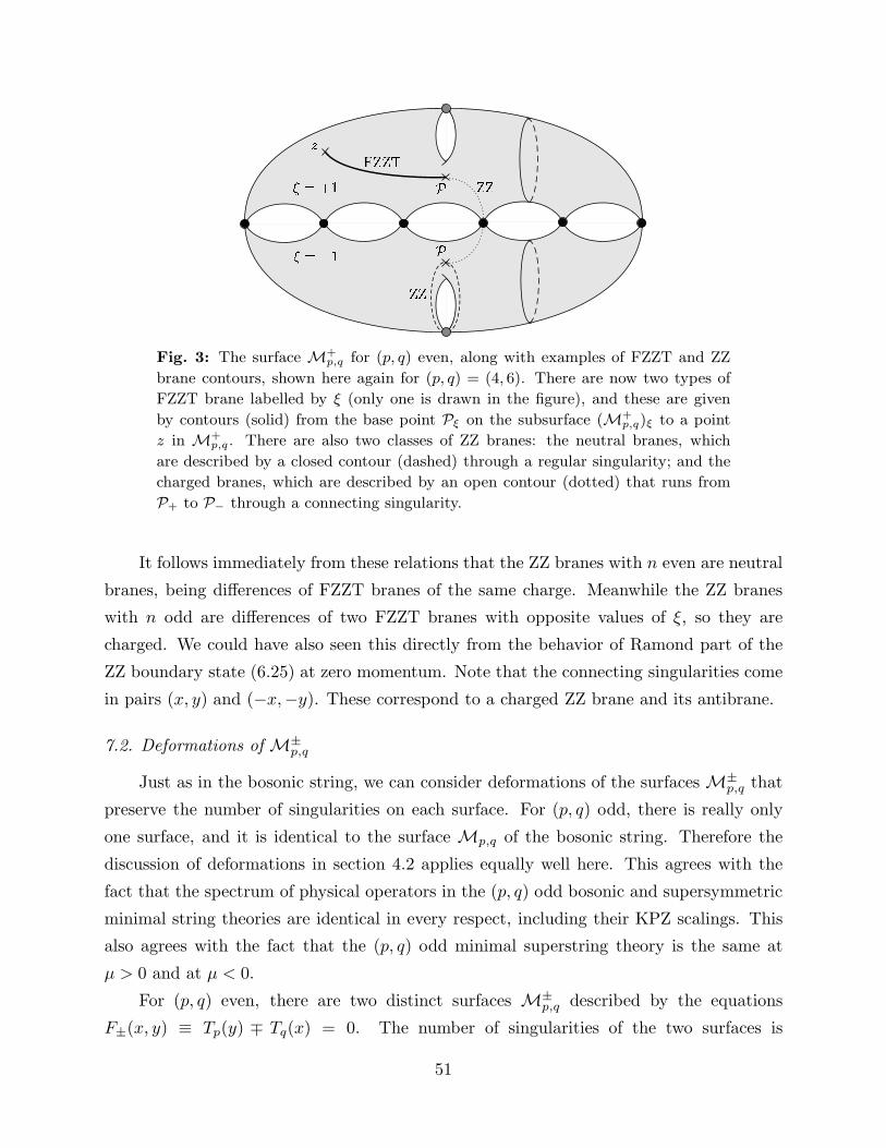
Fig. 3: The surface M+p,q for (p, q) even, along with examples of FZZT and ZZ

brane contours, shown here again for (p, q) = (4, 6). There are now two types of

FZZT brane labelled by ξ (only one is drawn in the figure), and these are given

by contours (solid) from the base point Pξ on the subsurface (M+p,q)ξ to a point

z in M+p,q . There are also two classes of ZZ branes: the neutral branes, which

are described by a closed contour (dashed) through a regular singularity; and the

charged branes, which are described by an open contour (dotted) that runs from

P+ to P− through a connecting singularity.

It follows immediately from these relations that the ZZ branes with n even are neutral

branes, being differences of FZZT branes of the same charge. Meanwhile the ZZ branes

with n odd are differences of two FZZT branes with opposite values of ξ, so they are

charged. We could have also seen this directly from the behavior of Ramond part of the

ZZ boundary state (6.25) at zero momentum. Note that the connecting singularities come

in pairs (x, y) and (−x,−y). These correspond to a charged ZZ brane and its antibrane.

7.2. Deformations of M±p,q

Just as in the bosonic string, we can consider deformations of the surfaces M±p,q that

preserve the number of singularities on each surface. For (p, q) odd, there is really only

one surface, and it is identical to the surface Mp,q of the bosonic string. Therefore the

discussion of deformations in section 4.2 applies equally well here. This agrees with the

fact that the spectrum of physical operators in the (p, q) odd bosonic and supersymmetric

minimal string theories are identical in every respect, including their KPZ scalings. This

also agrees with the fact that the (p, q) odd minimal superstring theory is the same at

µ > 0 and at µ < 0.

For (p, q) even, there are two distinct surfaces M±p,q described by the equations

F±(x, y) ≡ Tp(y) ∓ Tq(x) = 0. The number of singularities of the two surfaces is

51

(p−1)(q−1)±12 . By arguments analogous to those in section 4.2, we find that a complete

and independent basis for the deformations is given by

δr,sF±(x, y) = tr,s

(Uq−s−1(x)Ur−1(y) ∓ Up−r−1(y)Us−1(x)

)

1 ≤ r ≤ p , s ≤ q − 1 , qr − ps ≥ 0 .

(7.17)

Note the one essential difference between the deformations of M±p,q: for M+

p,q, the de-

formation with (r, s) = (p2 ,

q2) is not present, because the two terms in (7.17) are equal

and cancel. In other words, there is no singularity preserving deformation of M+p,q that

corresponds to the Ramond ground state.

For the η = −1 brane, this is precisely what is needed. For µ > 0, the brane is

described by M−p,q, which does have a deformation corresponding to the Ramond ground

state. Meanwhile for µ < 0, the brane is described by M+p,q, which does not have a

deformation corresponding to the Ramond ground state. This agrees with our study of the

0B spectrum in section 5, where we saw that the Ramond ground state in the (−1/2,−1/2)

picture was present for µ > 0 and not present for µ < 0.

Consider now the η = +1 brane. For µ > 0 there is no problem, because although the

Ramond ground state exists in the string theory, its deformation of the surface is zero. This

occurs for two reasons: the Liouville part of the tachyon one-point function vanishes for

the Ramond ground state, and the matter wavefunction also vanishes by (6.16). However,

for µ < 0 the surface M−p,q has a deformation with (r, s) = (p

2, q

2), but the Ramond ground

state does not exist in the (−1/2,−1/2) picture. We do not know what this deformation

corresponds to.

Finally, we can extend the bosonic string discussion of the effect a background with

many (m,n) ZZ branes to the superstring. Adding to the system Nm,n ∼ 1/gs ZZ branes

the singularity associated with the pinched cycle Am,n is opened up and as in (4.32),

∮

Am,n

ydx = gsNm,n . (7.18)

When the (m,n) D-brane is charged, this has the effect of adding flux to the system

which can be measured by an expression similar to (7.18). Indeed, in [24] the flux due to

charged D-branes was defined by such a contour integral, and its effect on the dynamics

was discussed.

52

8. Comparing the (p, q) odd supersymmetric and bosonic models

In this section, we will compare the bosonic and 0B supersymmetric minimal string

theories with (p, q) odd.

First, the two theories have the same spectrum of physical operators [24,33]. In

particular, they both have (p−1)(q−1)/2 tachyons, and their ground rings are isomorphic.

Moreover, since the µ-deformed ground ring multiplication is the same in both theories,

the arguments of section 2.2 and 5.2 imply that the tachyon N -point functions for N ≤ 3

are the same in the two theories. Both will be given essentially by the fusion rules in the

minimal model, which are the same as the fusion rules of the superminimal model. A more

interesting test of our conjecture would be to compare the general (N > 4) correlation

functions of the two theories. This might probe structure of the theories that goes beyond

their ground rings.

Second, as we saw in section 5, the (p, q) odd minimal superstring theories do not

have the Ramond ground state in their spectrum, for either sign of µ. Thus for these

models, worldsheet supersymmetry is always broken. Moreover, since the Ramond ground

state measures RR charge, it is not possible to define such a charge for the (p, q) odd

minimal superstring. These are of course both necessary conditions if the supersymmetric

and bosonic theories are to be the same.

The boundary states of the bosonic and supersymmetric models offer more opportu-

nities for comparison. As we saw in section 7.1, they are described by the same Riemann

surface Mp,q. Thus it is reasonable to expect the bosonic and supersymmetric theories to

have an identical set of FZZT and ZZ branes. We will not offer a detailed comparison, but

will instead focus on the simplest test: counting the total number of such states. In the

bosonic string, we found that the set of all FZZT branes reduced to a one-parameter family

(parametrized by σ or z) of FZZT branes with matter state (1, 1). We also found exactly

(p− 1)(q − 1)/2 independent ZZ branes distinguished by their Liouville label (m,n).

Compare this with the boundary states in the superstring. These states are in general

labelled by ξ = ±1 and η = ±1 in addition to their Liouville and matter labels. For

(p, q) odd, we suggested in section 6.2 that both ξ and η are redundant parameters. These

arguments were also motivated geometrically in section 7. Then assuming that there

is a reduction of the FZZT branes with general matter state to the FZZT branes with

(1, 1) matter state, as in the bosonic string, we find the same one-parameter family of

independent FZZT branes. We also find exactly (p − 1)(q − 1)/2 ZZ branes, as in the

53

bosonic string, again assuming the reduction in matter states. Clearly, it would be nice

to justify this assumption with an explicit computation. For this, we would need explicit

expressions for the matter wavefunctions.

We will see in the next section that the Riemann surface is precisely the surface that

defines the dual matrix model description. Therefore the bosonic and supersymmetric

(p, q) models have the same matrix model, and we expect them to agree to all orders in

string perturbation theory.

We will conclude this section with a list of further tests of our proposed duality that

should be carried out. The 0B superstring has a Z2 symmetry and orbifolding by it leads

to the 0A theory. It is not known whether an analogous construction exists in the bosonic

string. It also remains to understand what it means to have negative µ in the bosonic

string, since the superstring clearly exists for both signs of µ, and moreover it is invariant

under µ → −µ. Finally, a more detailed comparison of the boundary states should be

undertaken, using explicit formulas for the matter wavefunctions.

9. Relation to matrix models

Finally we come to discuss the connection to the dual matrix model. Clearly, the

matrix model description emerges from the Riemann surface Mp,q. The FZZT brane

corresponds to the macroscopic loop operator of the matrix model, with the x and y the

matrix eigenvalue and the resolvent, respectively. The analytic structure of Mp,q dictates

the critical behavior of the matrix model, which is the starting point of the double-scaling

limit.

It is known that there are many equivalent matrix model descriptions of the (p, q)

minimal string theories. The most natural descriptions for our purposes are Kostov’s loop

gas formalism [30-37] and the two-matrix model [38]. We will focus mainly on the latter.

However for actual calculations, especially in the conformal background, the former is often

more useful. The two-matrix model consists of two random N ×N hermitian matrices X

and Y , described by the partition function

Zmatrix =

∫dXdY exp

(−Ng

Tr (V1(X) + V2(Y ) −XY )

). (9.1)

In the planar N → ∞ limit, the eigenvalues of X and Y are described by a continuous

distribution which can be determined from the structure of the surface Mp,q. For instance,

54

when p = 2, the surface can be described as a two-sheeted cover of the complex plane.

Then the eigenvalues are localized to the branch cuts of the surface.

Important observables in the two-matrix model are the two resolvents, which are

derivatives of the loop operators:

R(x) ≡W ′(x) = Tr1

X − x, R(y) ≡ W ′(y) = Tr

1

Y − y. (9.2)

These resolvents were calculated in the equivalent loop-gas formalism [30-35] for the (p, q)

minimal string theories in the conformal background, and at least for the bosonic models

where (p, q) are relatively prime, they are given by the following expressions:

R(x) =(x+

√x2 − 1

)q/p

+(x−

√x2 − 1

)q/p

R(y) =(y +

√y2 − 1

)p/q

+(y −

√y2 − 1

)p/q

.

(9.3)

One can show that the two resolvents are inverses of one another; in fact this is a conse-

quence of the saddle-point equations of the two-matrix model. Thus we should identify

y = R(x) and x = R(y). Moreover, if we write x = cosh θ and y = coshφ, the equations

above become simply the equation Tp(y) − Tq(x) = 0 of our surface Mp,q. Therefore, the

eigenvalues x and y are the boundary cosmological constant and resolvent of the FZZT

brane, respectively. Since y = R(x) and x = R(y), we also identify the FZZT brane and

the dual brane with the two macroscopic loops built out of X and Y , respectively. The

fact that there are only two macroscopic loops in the two-matrix model also agrees well

with our results in section 3, where we found that there was only one type of FZZT brane

(and its dual), labelled by matter state (1, 1).

The picture is analogous for the superstring. For (p, q) odd, the matrix model is

the same as in the bosonic string, and in particular the expressions for the resolvents

are unchanged. This agrees with the fact that we find only one surface in the (p, q) odd

superstring, and moreover that it is the same surface as in the bosonic string. For (p, q)

even, there are two surfaces, so the two-matrix model description is more difficult. In

particular, for a given sign of µ, we can make only one of the surfaces starting from the

resolvents (9.2). Perhaps the other surface arises from a more complicated resolvent.

Identifying the coordinates (x, y) of Mp,q with the eigenvalues of X and Y also sug-

gests a way to go beyond tree-level in the minimal string theory. In section 4.1, we discussed

the sense in which x and y are conjugate variables. This has a natural interpretation in

55

the two-matrix model, where in the double-scaling limit the two matrices become the

pseudo-differential operators Q and P which satisfy the equation [8]:

[Q,P ] = ~ . (9.4)

This suggests that in order to quantize the minimal string theory, we should promote x

and y to operators and quantize the Riemann surface Mp,q [39,40]. This is a promising

avenue of investigation that we will leave for future work.

Another connection with the matrix model that we should mention is the relation

between matrix model operators and the operators of minimal string theory in the confor-

mal background (µ 6= 0). The natural basis of operators in the matrix model are simply

products of X and Y ; while the tachyons, ground ring elements, etc. are natural to use in

minimal string theory. The relations (2.30) and (2.32) in terms of Chebyshev polynomials

(and their counterparts in the superstring) tell us how to transform from one basis to

another. In [25], this change of basis was worked out in detail for the (p, q) = (2, 2m− 1)

minimal string theories, and in appendix B we check explicitly that our results are in com-

plete agreement. Our results on the µ-deformed ring elements, tachyons and macroscopic

loops generalize the work of [25] to all (p, q).

The most detailed picture we have is for theories with p = 2 which can be described

by a one-matrix model. Here we have a unified description of the bosonic models (q odd),

the supersymmetric models (q = 4k) and its generalizations (q = 4k+ 2). For the bosonic

models, the description is in terms of a one-matrix model with one cut. The curve is

2y2 = Tq(x) + 1 =

(T q+1

2(x) + T q−1

2(x))2

x+ 1, (9.5)

and the effective eigenvalue potential Veff (x) is obtained by integrating y with respect to

x [24]:√

2Veff (x) =T q+3

2(x) + T q+1

2(x)

(q + 2)√x+ 1

−T q−1

2(x) + T q−3

2(x)

(q − 2)√x+ 1

. (9.6)

On the other hand, the supersymmetric 0B models are represented by a one-matrix model,

which has two cuts for µ > 0 and no cuts for µ < 0 [66-68,24]. Here we have the curve

2y2 = η Tq(x) + 1 (9.7)

for the η = ±1 brane. For the η = −1 brane, we find

Veff (x)∣∣η=−1

=

(2q T q

2(x) − xU q

2−1(x))√

1 − x2

q2 − 4, (9.8)

56

while for the η = +1 brane the result is

Veff (x)∣∣η=+1

=T q

2 +1(x)

q + 2−T q

2−1(x)

q − 2. (9.9)

For example in pure supergravity, (p, q) = (2, 4) and the curve for the η = −1 brane

becomes y2 = −4x2(x2 − 1), while for η = 1 the curve is y2 = (2x2 − 1)2. In general,

we find that the curve has no cuts for η = +1 (it is polynomial in x) and has two cuts

starting at x = ±1 for η = −1. Thus the resolvent of the 0B matrix model in the positive

(negative) µ phase corresponds to the η = −1 (+1) brane. Evidently, only the η = −1

brane can be interpreted as the resolvent in the 0B matrix model.

Using a change of variables, we can also obtain the resolvents of the 0A matrix models

for the (2, 2k) theories. The change of variables is motivated by the fact that in 0A,

the natural variable is not the eigenvalue xB, but rather xA = x2B. If we think of the

resolvents for 0A and 0B as a one-forms on the Riemann surface, imposing that the one-

forms transform into one another results in yB dxB = yA dxA = 2yAxB dxB, so we find

xA = x2B , yA =

yB

2xB. (9.10)

Thus the resolvent of 0A can actually have a pole at xA = 0, a fact noticed in [24]. There

it was convenient to define the curve of 0A in terms of

yA ≡ 2xAyA = xByB . (9.11)

Using (9.10) and (9.11), we find the 0A curves:

2y2A = xA

(η T q

2

(2xA − 1

)+ 1). (9.12)

Again, for pure supergravity we recognize the resolvent of the 0A matrix model in the two

phases as the η = −1 brane. For positive µ (η = −1) it satisfies y2A = 4x2

A(1− xA) and for

negative µ (η = +1) it is y2A = xA(2xA − 1)2. Moreover, at least for pure supergravity, the

η = ±1 brane in 0A is the same as the η = ∓1 brane in 0B. As we have already seen, the

η = +1 0B brane cannot be described easily in the 0B language. Instead, it has a natural

description as the resolvent of the 0A theory.

The description in terms of the effective potential gives us a more physical understand-

ing of the ZZ branes in the one-matrix model. The singularities of the surface correspond

to points where y(x) = T ′q(x) = 0, i.e. the regular zeros of y. In terms of the effective

57

eigenvalue potential Veff (x), this is the statement that the singularities are local extrema

of Veff (x). Therefore the ZZ branes are matrix eigenvalues located at the zero-force points

of the effective potential. In order to create a ZZ brane, we must pull it out of the Fermi

sea, which corresponds to the branch cut of our surface. This is the meaning of the ZZ

brane as a contour integral: the integral pulls an eigenvalue from the Fermi sea onto the

singularity (zero-force point).

Note that the extrema of Veff (x) are not necessarily local maxima. Let us focus on

the bosonic models for concreteness, whose effective potential is given by (9.6). It is easy

to show that the principal (1, n) ZZ branes with n even (odd) lie at local minima (maxima)

of Veff , and moreover at these extrema, Veff takes the values

Veff (xn) ∼ (−1)n+1 sin2πn

2m− 1. (9.13)

Recall that the “Fermi level” of the perturbative vacuum is located at Veff = 0. Then

according to (9.13), all the minima of Veff lie below the Fermi sea. Apparently, all of these

models are slightly unstable to the tunneling of a small number of eigenvalues into the

minima of Veff .

This detailed discussion has so far been only for the one-matrix model. The picture

in the two matrix model is not nearly as complete. For example, it is not clear how to

obtain the 0A curves. Presumably, this can be done by considering a two-matrix model of

complex matrices. Also, a description in terms of an effective potential is lacking, although

some interesting proposals were advanced in [69]. In any event, we still expect that in some

sense the singularities of Mp,q are “zero-force” points of some effective potential.

The effect of adding order 1/gs ZZ branes on the Riemann surface has a natural

interpretation in the matrix model. As in [55,56], the contour integral (4.32)(7.18)

∮

Am,n

ydx = gsNm,n . (9.14)

measures the number of eigenvalues around (xmn, ymn). We again see that the matrix

model eigenvalues can be thought of as ZZ branes with the different (m,n) ZZ brane differ

by their position in the surface.

58

Acknowledgments:

We would like to thank C. Beasley, M. Douglas, I. Klebanov, D. Kutasov, J. Mal-

dacena, E. Martinec, J. McGreevy, G. Moore, S. Murthy, P. Ouyang, L. Rastelli and

E. Witten for useful discussions. The research of NS is supported in part by DOE grant

DE-FG02-90ER40542. The research of DS is supported in part by an NSF Graduate

Research Fellowship and by NSF grant PHY-0243680. Any opinions, findings, and conclu-

sions or recommendations expressed in this material are those of the author(s) and do not

necessarily reflect the views of the National Science Foundation.

Appendix A. The Backlund transformation and FZZT branes

The purpose of this appendix is to give a semiclassical, intuitive picture of the FZZT

branes using the Backlund transformation.

A.1. Bosonic Liouville theory

We start with the bosonic Liouville theory in a two-dimensional, Lorentzian signature

spacetime (our conventions are chosen to agree with [14]):

L =1

4π

((∂τφ)2 − (∂σφ)2 − 4πµe2bφ

). (A.1)

The most general classical solution to the equations of motion is given in terms of two

arbitrary functions A±(x±)

e2bφcl =1

πb2µ

∂+A+∂−A−

(A+ −A−)2, (A.2)

where x± = τ ± σ and ∂± = 12(∂τ ± ∂σ). The Backlund field is a free field which is defined

in terms of A±

φ =1

2blog

(∂+A

+

∂−A−

). (A.3)

Eliminating A± we find

∂σφ = ∂τ φ−√

4πµebφ cosh(bφ)

∂τφ = ∂σφ−√

4πµebφ sinh(bφ) ,(A.4)

or equivalently

±∂±φ = ∂±φ−√

4πµ

2eb(φ±φ) . (A.5)

59

The generating functional of this transformation is∫dσ

(φ∂σφ−

√4πµ

bebφ sinh(bφ)

). (A.6)

Alternatively, we can start from the transformation (A.4) or (A.5) and check that they are

compatible only if the appropriate equations of motion are satisfied

∂+∂−φ = −πbµe2bφ , ∂+∂−φ = 0 . (A.7)

It is straightforward to evaluate the energy momentum tensor

T±± = (∂±φ)2 − 1

b∂2±φ = (∂±φ)2 ∓ 1

b∂2±φ , (A.8)

where the second term is the improvement term (note that it is different for φ and φ).

Using the classical solution (A.2) and the energy momentum tensor (A.8), one can check

that[∂2+ − b2T++(φcl)

] 1ö+A+

=[∂2+ − b2T++(φcl)

] A+

ö+A+

= 0 , (A.9)

and therefore[∂2+ − b2T++(φcl)

]e−bφcl = 0 . (A.10)

In the quantum theory this is the statement that e−bφ has a null descendant. This null

vector is the basis for the exact solution of the quantum theory [11-13].

The first term in the transformation (A.5) shows that it is like a T-duality trans-

formation. Therefore, we expect that Dirichlet and Neumann boundary conditions are

exchanged. Indeed, the FZZT brane which is associated with the Neumann boundary

conditions

∂σφ = −2πbµBebφ (A.11)

becomes a Dirichlet brane in terms of φ withµB√µ

=1

b√π

cosh(bφ) . (A.12)

Note that (A.12) is the semiclassical (b → 0) limit of (3.3), before the rescaling of µ and

µB . Therefore we identify the Backlund field with the parameter πσ of the FZZT brane.

The fact that Dirichlet and Neumann boundary conditions are exchanged by the

Backlund transformation is also clear from the form of the energy momentum tensor T±±

of (A.8). Because of the improvement term Dirichlet boundary conditions of φ are not

conformally invariant. However, in terms of φ the improvement terms in T++ and T−−

have opposite values. Therefore, Neumann boundary conditions for φ are not conformally

invariant but Dirichlet boundary conditions are consistent. Equivalently, a would-be local-

ized D-brane at φ is expected to have mass proportional to eφ

b . Therefore, it is unstable

and is pushed to φ→ +∞. On the other hand a D-brane localized at φ is stable.

60

A.2. Minisuperspace wavefunctions

In the minisuperspace approximation we focus on the zero mode of φ. We can take as

a complete basis of states the eigestates of φ or the states with energy 12P 2. Their inner

products are

〈φ1|φ2〉 = δ(φ1 − φ2)

〈P1|P2〉 = πδ(P1 − P2)

〈φ|P 〉 =2(

πµb2

)− iPb

Γ(−2iP

b

) K 2iPb

(√4πµ

bebφ

)

= e2iPφ(1 + . . .) +(πµb2

)− 2iPb Γ

(2iP

b

)

Γ(−2iP

b

)e−2iPφ(1 + . . .) .

(A.13)

The states |P 〉 were normalized such that the incoming wave e2iPφ in 〈φ|P 〉 has weight

one. The coefficient in front of e−2iPφ is a pure phase and is the reflection amplitude.

The boundary states are eigenstates of φ. They satisfy

〈φ|φ〉 = e−2πµBebφ

, µB =

õ

b√π

cosh(bφ)

〈φ1|φ2〉 = −1

blog

[√4πµ

b

(cosh(bφ1) + cosh(bφ2)

)]+ const

= −1

blog

(2√

4πµ

bcosh

b(φ1 + φ2)

2cosh

b(φ1 − φ2)

2

)+ const

〈φ|p〉 =2

bΓ

(2iP

b

)(πµb2

)−i Pb

cos(Pφ) .

(A.14)

The additive constant in 〈φ1|φ2〉 is a nonuniversal infinite constant which is independent

of φ1,2. The wave function 〈φ|φ〉 can be derived using the generating functional (A.6)

after exchanging the role of τ and σ. Alternatively, we can derive it in a Euclidean

worldsheet. Note that the states |φ〉 are not orthonormal. This means that the canonical

transformation from φ to φ is not unitary. This fact is also the reason for the somewhat

unusual decomposition

|φ〉 =2

bπ

∫ ∞

0

dP cos(2Pφ)Γ

(−2iP

b

)(πµb2

) iPb |P 〉 . (A.15)

The fact that is the semiclassical limit of the Liouville part of the FZZT boundary state

(3.1) confirms our identification of the Backlund field with the parameter πσ of the FZZT

brane. It is interesting that if not for the factor of Γ(−2ip

b

) (πµb2

)i p

b , this would have meant

that φ is conjugate to p and |φ〉 is a standard position eigenstate. However, since this

factor depends only on p and not on φ, that conclusion is not completely wrong.

61

A.3. Supersymmetric Liouville theory

Now let us consider super-Liouville theory with a Euclidean worldsheet. We follow

the conventions of [23], except that here we rescale µ → µ/2. The covariant derivatives,

supercharges and algebra are

D =∂

∂θ+ θ∂ , D =

∂

∂θ+ θ∂ , {D,D} = 2∂ , {D,D} = 2∂

Q =∂

∂θ− θ∂ , Q =

∂

∂θ− θ∂ , {Q,Q} = −2∂ , {Q,Q} = −2∂

(A.16)

with all other (anti)commutators vanishing. We define z = x+ iy, z = x− iy and therefore

∂ = (∂x − i∂y)/2, ∂ = (∂x + i∂y)/2. Finally, the integration measure is∫d2zd2θ =

2∫dxdydθdθ. The action for

Φ = φ+ iθψ + iθψ + iθθF (A.17)

is the super-Liouville action

S =1

4π

∫d2zd2θ

[DΦDΦ + iµebΦ

]. (A.18)

The Backlund transformation in super-Liouville theory [70,71] is

DΦ = DΦ + ξb√|µ|Γe b

2 (Φ+Φ)

DΦ = −DΦ − ξζb√|µ|Γe b

2 (Φ−Φ)

DΓ = −iξ√

|µ|4e

b2 (Φ+Φ)

DΓ = −iξζ√

|µ|4e

b2 (Φ−Φ)

ζ = sign(µ) ,

(A.19)

where Γ is a fermionic superfield (Γ2 = 0), and Φ is the Backlund field. (We have rescaled

the variables to agree with the conventions of [23].) The parameter ξ = ±1 implements

the (−1)FL symmetry, as discussed in section 6.1. It is straightforward to check that the

integrability conditions for (A.19) are the equations of motion

DDΦ +iµb

2ebΦ = 0

DDΦ = 0

DDΓ − iµb2

8ebΦΓ = 0 ,

(A.20)

62

i.e. Φ satisfies the equation of motion of (A.18), and Φ is free.

The energy momentum tensor superfield is

T = DΦD2Φ − 1

bD3Φ = DΦD2Φ − 1

bD3Φ

T = DΦD2Φ − 1

bD

3Φ = DΦD

2Φ +

1

bD

3Φ .

(A.21)

The second term is the improvement term. It has the same sign in T and T when expressed

in terms of Φ, but it has opposite signs in T and T when expressed in terms of Φ. The

fermionic superfield Γ does not contribute to the energy momentum tensor.

The FZZT branes are D0-branes of Φ; i.e. the Backlund field satisfies Dirichlet bound-

ary conditions

DtΦ = (D + ηD)Φ = 0 , (A.22)

where η = ±1 denotes the preserved subspace of superspace: θ = ηθ. The opposite signs

of the improvement term in T and T when expressed in terms of Φ (A.21), make these

boundary conditions conformal (conversely, Neumann boundary conditions on Φ are not

consistent). From (A.19) we find the boundary conditions of the other fields

DnΦ = (D − ηD)Φ = 2bµBΓeb2Φ

DtΓ = (D + ηD)Γ = −iµBeb2Φ ,

(A.23)

where

µB =

{ξ√|µ| cosh( b

2 Φ) η = +1

ξ√|µ| sinh( b

2 Φ) η = −1(A.24)

with η = ζη. This expression for µB is the semiclassical limit of (6.13). Thus, as in the

bosonic string, we are led to identify the Backlund field with the parameter σ of the FZZT

brane. Note also that the equations (A.23) are the boundary equations of motion when

we add to the action (A.18) the boundary term

Sbry =1

2π

∮dxdθt

(ΓDtΓ + 2iµBΓe

b2Φ)

=1

2π

∮dx[−γ∂xγ − f2 − µB

(bγ(ψ + ηψ)e

b2 φ + 2fe

b2 φ)]

=1

2π

∮dx[−γ∂xγ − µB b γ(ψ+ ηψ)e

b2φ + µ2

B ebφ],

(A.25)

where Γ = γ + iθtf is a fermionic superfield at the boundary.

63

A.4. Minisuperspace wavefunctions

We denote by |φ±〉 and |P±〉 the states with the two different fermion number in

the R sector and by |φ0〉 and |P0〉 the states in the NS sectors. Following [23] the wave

functions are expressed in terms of z = |µ|ebφ. Let us assume first that µ is positive

(ζ = sign(µ) = +1). Then the wavefunctions are9

〈φ1 ± |φ2±〉 = δ(φ1 − φ2)

〈φ10|φ20〉 = δ(φ1 − φ2)

〈P1 ± |P2±〉 = 2πδ(P1 − P2)

〈P10|P20〉 = 2πδ(P1 − P2)

ΨP±(φ) = 〈φ± |P±〉 =2

Γ(− iP

b + 12

)( |µ|

4

)− iPb √

z(K iP

b− 1

2(z) ±K iP

b+ 1

2(z))

= eiPφ (1 + O(z)) ± Γ(

iPb

+ 12

)

Γ(− iP

b + 12

)( |µ|

4

)− 2iPb

e−iPφ (1 + O(z))

ΨP0 = 〈φ0|P0〉 =2

Γ(− iP

b

)( |µ|

4

)− iPb

K iPb

(z)

= eiPφ (1 + O(z)) − Γ(1 + iPb

)

Γ(1 − iP

b

)( |µ|

4

)− 2iPb

e−iPφ (1 + O(z)) .

(A.26)

The wavefunctions satisfy

(z∂z ± z)ΨP±(z) =iP

bΨP∓(z)

(−(z∂z)

2 + z2 − P 2

b2

)ΨP0(z) = 0 .

(A.27)

When µ changes sign z which is defined in terms of |µ| does not change. Therefore

the equations (A.27) are unchanged. However, since these equations are derived from the

action of the supercharges, the term linear in z must change sign. This means that the

wavefunctions ΨP±(z) have the same functional form when µ changes sign but they occur

for the states with opposite fermion number; i.e.

〈φ± |P±〉 = ΨP,±ζ(z) . (A.28)

9 We reversed the ± label of ΨP± and changed the normalization of the wavefunctions relative

to [23] to have the coefficient of eiP φ in the wavefunctions normalized to one.

64

In order to study D-branes we need eigenstates of φ. In the R sector they are |φ±〉and in the NS sector |φ0〉. After integrating out the various fermions as in [23], we have

〈φ0|φ0〉 = e−z cosh(bφ)

〈φ± |φ±〉 =√ze−z cosh(bφ)

(e

bφ

2 ± ζe−bφ

2

)

〈φ0|P0〉 =2

b

( |µ|4

)− iPb

Γ

(iP

b

)cos(Pφ)

〈φ± |P±〉 =2

b

( |µ|4

)− iPb

Γ

(iP

b+

1

2

)(e−iP φ ± ζeiP φ

).

(A.29)

From these we derive the decompositions

|φ0〉 =1

bπ

∫ ∞

0

dP cos(Pφ)Γ

(− iPb

)( |µ|4

) iPb

|P0〉

|φ±〉 =1

bπ

∫ ∞

0

dP(eiP φ ± ζe−iP φ

)Γ

(− iPb

+1

2

)( |µ|4

) iPb

|P±〉 .(A.30)

These formulas for the boundary states agree with the semiclassical limit of (6.12).

Appendix B. Tests with the one-matrix model

In this appendix, we will study in detail the (2, 2m−1) bosonic minimal models, which

can be described very simply in terms of the mth critical point of a one-matrix model.

This will serve as a useful check of the general analysis of the bosonic (p, q) models in

sections 3 and 4 and the discussion of the matrix model in section 9. In the one matrix

model, there is only one resolvent, so we will focus on the FZZT brane and not its dual.

The resolvent is given by (9.5) with q = 2m− 1:

ym = (√µ)m−1/2Tm(x) + Tm−1(x)√

1 + x, (B.1)

where here we have restored the overall power of µ in front of y for the purposes of the

present discussion. Our goal will be to explicitly confirm (B.1) using the one-matrix model.

The method will be as follows. Turning on µ in the minimal string theory corresponds to

turning on a specific set of scaling perturbations in the matrix model. Using the techniques

of [25], we can perform the change of basis from µ to scaling perturbations of the matrix

model, and then explicitly compute the resolvent at non-zero µ, confirming (B.1).

65

Exactly at the mth critical point of the one-matrix model, the resolvent takes the

form y = (√µ)m−1/2xm−1/2(x − b)1/2. A general perturbation around the mth critical

point can be written as

y =

m∑

j=1

tjyj , (B.2)

where the tj are the couplings to the jth matrix model scaling operator, and the yj are

given by (see e.g. section 2.2 of [10]):

yj(x) =b1/2(

√µ)j−1/2

B(j, 12)

∫ a

x

ds (s− x)−1/2sj−1 . (B.3)

Here we are using the standard “Gelfand-Dikii” normalization of the couplings tj , so that

the string equation takes the form∑

j

tjRj [u] = 0 . (B.4)

Now, in order to compare with the continuum description in the “conformal background,”

i.e. with a fixed cosmological constant µ, we must express the tj in terms of µ. Explicit

formulas for this change of basis were derived in [25]:

tm−2p =cm−2p

am−2pµp

cm−2p =(−1)m+1π√

8

2m−2p

(m− 2p)! p ! Γ(p−m+ 32)

am−2p =(−1)m

22(m−2p)

(2m− 4p− 1m− 2p

).

(B.5)

Here ak is the leading coefficient of the Gelfand-Dikii polynomial Rk[u], i.e. Rk[u] =

akuk + . . .. We must include this factor when using the results of [25], because there a

slightly different normalization of the couplings tj was used, in which the (genus zero)

string equation has the form∑

i tjuj = 0. After some gamma function manipulations, we

obtain the following simplified form of tm−2p:

tm−2p =(−1)m+1

√2π

4(m− p)2 − 1

2m−2p+1

B(p+ 1,−12−m+ p)

µp . (B.6)

Substituting our formula for tj in (B.2), we find the form of the resolvent in the conformal

background:

y(x) = (−1)m+1b1/2(√µ)m−1/2

√2π

∫ a

x

ds (s− x)−1/2×

[m−12 ]∑

p=0

1

4(m− p)2 − 1

2m−2p+1

B(m− 2p, 12)B(p+ 1, p−m− 1

2)sm−2p−1 .

(B.7)

66

Using the identity

(−1)p+122m−2p

B(m− 2p, 12)B(p+ 1, p−m− 1

2)

=(4(m− p)2 − 1

)( 2m− 2p− 2m− 1

)(m− 1p

)(B.8)

in (B.7), we obtain

y(x) = (−1)mb1/2(√µ)m−1/2

√2π

∫ a

x

ds (s− x)−1/2×

1

2m−1

[m−12 ]∑

p=0

(−1)p

(2m− 2p− 2

m− 1

)(m− 1p

)sm−2p−1 .

(B.9)

We recognize the sum in (B.9) as an explicit form of the Legendre polynomial Pm−1(x).

Furthermore, the integral can be evaluated using standard tables assuming a = −1. Thus

we arrive at the final form of the matrix model curve:

y(x) = b1/2(−1)m+1√

2π(√µ)m−1/2

∫ x

−1

ds (s− x)−1/2Pm−1(s)

=(−1)m

√8π

2m− 1ib1/2(

√µ)m−1/2

(Tm (x) + Tm−1 (x)√

1 + x

),

(B.10)

which is indeed in exact agreement with the continuum prediction (B.1), up to an irrelevant

overall normalization that can be absorbed into the definition of b.

67

References

[1] F. David, “Planar Diagrams, Two-Dimensional Lattice Gravity And Surface Models,”

Nucl. Phys. B 257, 45 (1985).

[2] V. A. Kazakov, “Bilocal Regularization Of Models Of Random Surfaces,” Phys. Lett.

B 150, 282 (1985).

[3] V. A. Kazakov, A. A. Migdal and I. K. Kostov, “Critical Properties Of Randomly

Triangulated Planar Random Surfaces,” Phys. Lett. B 157, 295 (1985).

[4] J. Ambjorn, B. Durhuus and J. Frohlich, “Diseases Of Triangulated Random Surface

Models, And Possible Cures,” Nucl. Phys. B 257, 433 (1985).

[5] M. R. Douglas and S. H. Shenker, “Strings In Less Than One-Dimension,” Nucl. Phys.

B 335, 635 (1990).

[6] D. J. Gross and A. A. Migdal, “Nonperturbative Two-Dimensional Quantum Gravity,”

Phys. Rev. Lett. 64, 127 (1990).

[7] E. Brezin and V. A. Kazakov, “Exactly Solvable Field Theories Of Closed Strings,”

Phys. Lett. B 236, 144 (1990).

[8] M. R. Douglas, “Strings In Less Than One-Dimension And The Generalized K-D-V

Hierarchies,” Phys. Lett. B 238, 176 (1990).

[9] P. Ginsparg and G. W. Moore, “Lectures On 2-D Gravity And 2-D String Theory,”

arXiv:hep-th/9304011.

[10] P. Di Francesco, P. Ginsparg and J. Zinn-Justin, “2-D Gravity and random matrices,”

Phys. Rept. 254, 1 (1995) [arXiv:hep-th/9306153].

[11] H. Dorn and H. J. Otto, “Some conclusions for noncritical string theory drawn from

two and three point functions in the Liouville sector,” arXiv:hep-th/9501019.

[12] J. Teschner, “On the Liouville three point function,” Phys. Lett. B 363, 65 (1995)

[arXiv:hep-th/9507109].

[13] A. B. Zamolodchikov and A. B. Zamolodchikov, “Structure constants and confor-

mal bootstrap in Liouville field theory,” Nucl. Phys. B 477, 577 (1996) [arXiv:hep-

th/9506136].

[14] V. Fateev, A. B. Zamolodchikov and A. B. Zamolodchikov, “Boundary Liouville field

theory. I: Boundary state and boundary two-point function,” arXiv:hep-th/0001012.

[15] J. Teschner, “Liouville theory revisited,” Class. Quant. Grav. 18, R153 (2001)

[arXiv:hep-th/0104158].

[16] A. B. Zamolodchikov and A. B. Zamolodchikov, “Liouville field theory on a pseudo-

sphere,” arXiv:hep-th/0101152.

[17] J. McGreevy and H. Verlinde, “Strings from tachyons: The c = 1 matrix reloaded,”

arXiv:hep-th/0304224.

[18] E. J. Martinec, “The annular report on non-critical string theory,” arXiv:hep-

th/0305148.

68

[19] I. R. Klebanov, J. Maldacena and N. Seiberg, “D-brane decay in two-dimensional

string theory,” JHEP 0307, 045 (2003) [arXiv:hep-th/0305159].

[20] J. McGreevy, J. Teschner and H. Verlinde, “Classical and quantum D-branes in 2D

string theory,” arXiv:hep-th/0305194.

[21] S. Y. Alexandrov, V. A. Kazakov and D. Kutasov, “Non-perturbative effects in matrix

models and D-branes,” JHEP 0309, 057 (2003) [arXiv:hep-th/0306177].

[22] I. K. Kostov, B. Ponsot and D. Serban, “Boundary Liouville theory and 2D quantum

gravity,” arXiv:hep-th/0307189.

[23] M. R. Douglas, I. R. Klebanov, D. Kutasov, J. Maldacena, E. Martinec and N. Seiberg,

“A new hat for the c = 1 matrix model,” arXiv:hep-th/0307195.

[24] I. R. Klebanov, J. Maldacena and N. Seiberg, “Unitary and complex matrix models

as 1-d type 0 strings,” arXiv:hep-th/0309168.

[25] G. W. Moore, N. Seiberg and M. Staudacher, “From loops to states in 2-D quantum

gravity,” Nucl. Phys. B 362, 665 (1991).

[26] B. H. Lian and G. J. Zuckerman, “New Selection Rules And Physical States In 2-D

Gravity: Conformal Gauge,” Phys. Lett. B 254, 417 (1991).

[27] E. Witten, “Ground ring of two-dimensional string theory,” Nucl. Phys. B 373, 187

(1992) [arXiv:hep-th/9108004].

[28] T. Banks, M. R. Douglas, N. Seiberg and S. H. Shenker, “Microscopic And Macroscopic

Loops In Nonperturbative Two-Dimensional Gravity,” Phys. Lett. B 238, 279 (1990).

[29] G. W. Moore and N. Seiberg, “From loops to fields in 2-D quantum gravity,” Int. J.

Mod. Phys. A 7, 2601 (1992).

[30] I. K. Kostov, “Multiloop correlators for closed strings with discrete target space,”

Phys. Lett. B 266, 42 (1991).

[31] K. Hosomichi, “Bulk-boundary propagator in Liouville theory on a disc,” JHEP 0111,

044 (2001) [arXiv:hep-th/0108093].

[32] B. Ponsot, “Liouville theory on the pseudosphere: Bulk-boundary structure constant,”

arXiv:hep-th/0309211.

[33] C. V. Johnson, “Non-perturbative string equations for type 0A,” arXiv:hep-th/0311129.

[34] I. K. Kostov, “Loop Amplitudes For Nonrational String Theories,” Phys. Lett. B 266,

317 (1991).

[35] I. K. Kostov, “Strings with discrete target space,” Nucl. Phys. B 376, 539 (1992)

[arXiv:hep-th/9112059].

[36] I. K. Kostov, “Loop space Hamiltonian for c ≤ 1 open strings,” Phys. Lett. B 349,

284 (1995) [arXiv:hep-th/9501135].

[37] I. K. Kostov, “Boundary correlators in 2D quantum gravity: Liouville versus discrete

approach,” Nucl. Phys. B 658, 397 (2003) [arXiv:hep-th/0212194].

[38] J. M. Daul, V. A. Kazakov and I. K. Kostov, “Rational theories of 2-D gravity from

the two matrix model,” Nucl. Phys. B 409, 311 (1993) [arXiv:hep-th/9303093].

69

[39] G. W. Moore, “Geometry Of The String Equations,” Commun. Math. Phys. 133, 261

(1990).

[40] G. W. Moore, “Matrix Models Of 2-D Gravity And Isomonodromic Deformation,”

Prog. Theor. Phys. Suppl. 102, 255 (1990).

[41] M. Aganagic, R. Dijkgraaf, A. Klemm, M. Marino and C. Vafa, “Topological Strings

and Integrable Hierarchies,” arXiv:hep-th/0312085.

[42] N. Seiberg, “Notes On Quantum Liouville Theory And Quantum Gravity,” Prog.

Theor. Phys. Suppl. 102, 319 (1990).

[43] B. H. Lian and G. J. Zuckerman, “Semiinfinite Homology And 2-D Gravity. 1,” Com-

mun. Math. Phys. 145, 561 (1992).

[44] B. H. Lian, “Semiinfinite Homology And 2-D Quantum Gravity,” UMI-92-21392,

Ph.D. Thesis, Yale University (1991).

[45] D. Kutasov, E. J. Martinec and N. Seiberg, “Ground rings and their modules in 2-D

gravity with c ≤ 1 matter,” Phys. Lett. B 276, 437 (1992) [arXiv:hep-th/9111048].

[46] P. Di Francesco and J. B. Zuber, “Fusion potentials. 1,” J. Phys. A 26, 1441 (1993)

[arXiv:hep-th/9211138].

[47] C. Imbimbo, “New modular representations and fusion algebras from quantized

SL(2,R) arXiv:hep-th/9301031.

[48] C. Imbimbo, “Polynomial Fusion Rings From Sl(2,R) Chern-Simons Theory,” Phys.

Lett. B 308, 51 (1993).

[49] P. Di Francesco and D. Kutasov, “Unitary Minimal Models Coupled To 2-D Quantum

Gravity,” Nucl. Phys. B 342, 589 (1990).

[50] M. Goulian and M. Li, “Correlation Functions In Liouville Theory,” Phys. Rev. Lett.

66, 2051 (1991).

[51] P. Di Francesco and D. Kutasov, “World sheet and space-time physics in two-

dimensional (Super)string theory,” Nucl. Phys. B 375, 119 (1992) [arXiv:hep-

th/9109005].

[52] J. L. Cardy, “Boundary Conditions, Fusion Rules And The Verlinde Formula,” Nucl.

Phys. B 324, 581 (1989).

[53] S. Alexandrov, “(m,n) ZZ branes and the c = 1 matrix model,” arXiv:hep-th/0310135.

[54] E. J. Martinec, G. W. Moore and N. Seiberg, “Boundary operators in 2-D gravity,”

Phys. Lett. B 263, 190 (1991).

[55] R. Dijkgraaf and C. Vafa, “A perturbative window into non-perturbative physics,”

arXiv:hep-th/0208048.

[56] F. Cachazo, M. R. Douglas, N. Seiberg and E. Witten, “Chiral rings and anomalies

in supersymmetric gauge theory,” JHEP 0212, 071 (2002) [arXiv:hep-th/0211170].

[57] P. Di Francesco, H. Saleur and J. B. Zuber, “Generalized Coulomb Gas Formalism For

Two-Dimensional Critical Models Based On SU(2) Coset Construction,” Nucl. Phys.

B 300, 393 (1988).

70

[58] R. C. Rashkov and M. Stanishkov, “Three-point correlation functions in N=1 Super

Lioville Theory,” Phys. Lett. B 380, 49 (1996) [arXiv:hep-th/9602148].

[59] R. H. Poghosian, “Structure constants in the N = 1 super-Liouville field theory,” Nucl.

Phys. B 496, 451 (1997) [arXiv:hep-th/9607120].

[60] T. Fukuda and K. Hosomichi, “Super Liouville theory with boundary,” Nucl. Phys. B

635, 215 (2002) [arXiv:hep-th/0202032].

[61] C. Ahn, C. Rim and M. Stanishkov, “Exact one-point function of N=1 super-Liouville

theory with boundary,” Nucl. Phys. B 636, 497 (2002) [arXiv:hep-th/0202043].

[62] S. Panda and S. Roy, “BRST cohomology ring in c(M) < 1 NSR string theory,” Phys.

Lett. B 358, 229 (1995) [arXiv:hep-th/9507054].

[63] P. Bouwknegt, J. G. McCarthy and K. Pilch, “Ground ring for the 2-D NSR string,”

Nucl. Phys. B 377, 541 (1992) [arXiv:hep-th/9112036].

[64] K. Itoh and N. Ohta, “Spectrum of two-dimensional (super)gravity,” Prog. Theor.

Phys. Suppl. 110, 97 (1992) [arXiv:hep-th/9201034].

[65] K. Itoh and N. Ohta, “BRST cohomology and physical states in 2-D supergravity

coupled to c ≤ 1 matter,” Nucl. Phys. B 377, 113 (1992) [arXiv:hep-th/9110013].

[66] D. J. Gross and E. Witten, “Possible Third Order Phase Transition In The Large N

Lattice Gauge Theory,” Phys. Rev. D 21, 446 (1980).

[67] V. Periwal and D. Shevitz, “Unitary Matrix Models As Exactly Solvable String The-

ories,” Phys. Rev. Lett. 64, 1326 (1990).

[68] C. Crnkovic, M. R. Douglas and G. W. Moore, “Loop equations and the topological

phase of multi-cut matrix models,” Int. J. Mod. Phys. A 7, 7693 (1992) [arXiv:hep-

th/9108014].

[69] V. A. Kazakov and A. Marshakov, “Complex curve of the two matrix model and its

tau-function,” J. Phys. A 36, 3107 (2003) [arXiv:hep-th/0211236].

[70] M. Chaichian and P. P. Kulish, “On The Method Of Inverse Scattering Problem And

Backlund Transformations For Supersymmetric Equations,” Phys. Lett. B 78, 413

(1978).

[71] E. D’Hoker, “Classical And Quantal Supersymmetric Liouville Theory,” Phys. Rev.

D 28, 1346 (1983).

71