arX

iv:h

ep-p

h/96

0746

5v1

29

Jul 1

996

FSU-HEP-960801

CONSTRAINTS ON

THE MINIMAL SUPERGRAVITY MODELFROM NON-STANDARD VACUA

Howard Baer, Michal Brhlik and Diego CastanoDepartment of Physics, Florida State University, Tallahassee, FL 32306 USA

(July 14, 2011)

Abstract

We evaluate regions of parameter space in the minimal supergravity model

where “unbounded from below” (UFB) or charge or color breaking minima

(CCB) occur. Our analysis includes the most important terms from the 1-

loop effective potential. We note a peculiar discontinuity of results depending

on how renormalization group improvement is performed: One case leads

to a UFB potential throughout the model parameter space, while the other

typically agrees quite well with similar calculations performed using only the

tree level potential. We compare our results with constraints from cosmology

and naturalness and find a preferred region of parameter space which implies

mg<∼ 725 GeV, mq

<∼ 650 GeV, mW1

<∼ 225 GeV and mℓR

<∼ 220 GeV. We

discuss the consequences of our results for supersymmetry searches at various

colliding beam facilities.

Typeset using REVTEX

1

I. INTRODUCTION

The Minimal Supersymmetric Standard Model (MSSM) is one of the leading candidatemodels [1] for physics beyond the Standard Model (SM). In this theory, one begins withthe SM particles (but with two Higgs doublets to ultimately ensure anomaly cancellation);supersymmetrization then leads to partner particles for each SM particle which differ by spin-1

2. Supersymmetry breaking is implemented by adding explicit soft supersymmetry breaking

terms. This procedure leads to a particle physics model with >∼ 100 free parameters, whichought to be valid at the weak scale.

To reduce the number of free parameters, one needs a theory of how the soft SUSYbreaking terms arise, i.e., how supersymmetry is broken. In the minimal supergravity model(SUGRA) [2], supersymmetry is spontaneously broken via a hidden sector field vacuumexpectation value (VEV), and the SUSY breaking is communicated to the visible sector viagravitational interactions. For a flat Kahler metric and common gauge kinetic functions, thisleads to a common scalar mass m0, a common gaugino mass m1/2, and common trilinearand bilinear terms A0 and B0 at some high scale MGUT − MPl, where the former choiceis usually taken due to apparent gauge coupling unification at ∼ 2 × 1016 GeV. The highscale mass terms and couplings are then linked to weak-scale values via renormalizationgroup evolution. Electroweak symmetry breaking [3], which is hidden at high scales, isthen induced by the large top-quark Yukawa coupling, which drives one of the Higgs fieldmasses to a negative value. Minimization of the scalar potential allows one to effectivelyreplace B by tanβ and express the magnitude (but not the sign) of the Higgsino mass µ interms of MZ . The resulting parameter space of this model is thus usually given by the set(m0, m1/2, A0, tanβ, and sign(µ)).

Not all values of the above 4 + 1 dimensional parameter space of the minimal SUGRAmodel are allowed. For instance, the top and bottom Yukawa couplings are driven to infinitysomewhere between MZ and MGUT for tanβ <∼ 1.5 and >∼ 50 (depending on the value of mt)[4]. For other parameter choices, the lightest chargino or lightest slepton (or top squark)can be the lightest SUSY particle, which would violate limits on, for instance, heavy exoticnuclei. For yet other parameter choices, electroweak symmetry breaking leads to the wrongvalue of MZ , so these parameter choices are ruled out. In addition, there are cosmologicalbounds from the relic density of neutralinos produced in the Big Bang [5]. Requiring theuniverse to be older than ∼ 10 billion years leads to only a subset of the parameter spacebeing allowed, although this bound could be evaded by allowing for a small amount of R-parity violation. Finally, certain regions of parameter space are rejected by negative searchesfor sparticles at colliding beam experiments, such as those at LEP and the Fermilab Tevatron[6].

An additional constraint on minimal SUGRA parameters can be obtained by requiringthat the global minimum of the scalar potential is indeed the minimum that leads to ap-propriate electroweak symmetry breaking. In the SM, there is only a single direction inthe field space of the scalar potential, so appropriate electroweak symmetry breaking canbe assured. For the MSSM, the plethora of new scalar fields which are introduced leads tomany possible directions in field space where minima could develop which are deeper thanthe standard minimum. Thus, parameter choices which lead to deeper minima should beexcluded as well, since they would lead to a universe with a non-standard vacuum.

2

Constraints along the preceeding lines were developed in Refs. [7] in the early 1980’s,using the renormalization group improved tree level effective potential. It was noted byGamberini et. al. [8] that the renormalization group improved tree potential was subject tolarge variations due to uncertainty in the correct scale choice Q at which it was evaluated.Inclusion of 1-loop corrections served to ameliorate this condition. Recently, Casas, Lleyda,and Munoz [9] have made a systematic survey of all possible dangerous directions in scalarfield space that can potentially lead to minima deeper than the standard one. These havebeen categorized as field directions that are either unbounded from below (at tree level)(UFB) or that lead to charge or color-breaking (CCB) minima. For simplicity, their analysisuses the tree-level scalar potential but evaluated at an optimized mass scale where 1-loopcorrections ought to be only a small effect. Working within the minimal SUGRA model,they considered models with B0 = A0−m0 or B0 = 2m0 and showed that significant regionsof parameter space could be excluded via this method.

In the present work, one of our main goals is to delineate the parameter space regionswhere non-standard potential minima develop in such a manner as to facilitate comparisonswith other constraints, including recently calculated results on the neutralino relic density[10] and parameter space regions favored by fine-tuning considerations [11]. In addition,expectations for supersymmetry at LEP2 [12], the Tevatron MI and TeV33 upgrades [13],the LHC [14], and NLC [15] have been calculated within the minimal SUGRA framework.We also compare the non-standard vacuum constraints with the various collider expectationsand draw some conclusions. For instance, combining the non-standard vacuum constraintswith the most favored parameter space regions from fine-tuning and cosmology suggests thatthe Fermilab TeV33 upgrade stands a high chance to discover SUSY via the W1Z2 → 3ℓsignal!

In the present work, we also adopt a somewhat different calculational scheme from thatemployed in Ref. [9]. For all field directions considered, we implement renormalization group(RG) improvement to calculate the 1-loop effective potential. We find that the inclusionof the 1-loop correction has important consequences. The 1-loop correction almost alwaysrepresents a significant contribution to the tree level potential. Nevertheless, our overallresults agree very well with those of [9] for a “proper” choice in RG improvement scheme.For reference, we shall call this the “α-case,” and it represents our main results. However,for other choices of RG improvement, we find that the 1-loop correction can be so dominantas to lead to unbounded from below (UFB) potentials everywhere in parameter space: Werefer to this as the “ω-case.” Because this is a multi-scale problem, it is not entirely clearhow to proceed with RG improvement, and it is this ambiguity that leads to the two casesabove. The validity of our results hinge on two main assumptions. The first concerns theadequacy of cutting the expansion at 1-loop. It is beyond the present analysis to ascertainthe significance of the 2-loop contribution in any of the cases considered. However, becauseof the dependence of our results on the details of RG improvement, we believe that the2-loop contribution may be important. Secondly, we have only included the contribution ofthe top-stop sector in our calculations of the 1-loop correction. It remains to be determinedif the inclusion of the other fields will significantly affect the results.

We note briefly that the work of [16] and [17] advances the idea that we may indeed existin a false vacuum and that the tunnelling rate from our present vacuum to a UFB or CCBvacuum might be small relative to the age of the universe. In this case, the following derived

3

constraints would not be meaningful. Such a philosophy must, however, be reconciled [18]with the fact that we live in a world in which the cosmological constant either vanishes oris extremely small. This is empirical, albeit indirect, evidence for some mechanism whichseeks to enforce the principle that “the cosmological constant of the true vacuum is zero.” Itis difficult to conceive of circumstances where we could tenably entertain both the idea thatwe are living in a false vacuum and the idea that the smallness of the cosmological constanthas a natural solution, since this would require a principle which would set the cosmologicalconstant to zero in a false, broken vacuum while simultaneously leaving the true, brokenvacuum with a large negative cosmological constant.

The organization of the paper is as follows. In Section II, we review the MSSM scalarpotential and give a brief summary of the UFB and CCB directions delineated in Ref. [9].In Section III, we present our calculational procedure and in Sec. IV present results ofour scans over SUGRA parameter space. In Section V we give a brief summary of ourresults. Detailed formulae for the effective potential in various UFB and CCB directionsare included in Appendix A, while some computationally useful formulae for evaluating theeffective potential in the limit of large VEVs is presented in Appendix B.

II. DANGEROUS DIRECTIONS IN FIELD SPACE

The scalar potential of the MSSM can be written as

V = VF + VD + Vsoft , (2.1)

where

VF =∑

α

∣∣∣∣∣∂W

∂φα

∣∣∣∣∣

2

=

∣∣∣∣∣∑

i

uiyuiQi + µΦd

∣∣∣∣∣

2

+

∣∣∣∣∣∑

i

(ydi

diQi + yeieiLi

)+ µΦu

∣∣∣∣∣

2

+∑

i

|yuiΦuQi|2 +

∑

i

|ydiΦdQi|2 +

∑

i

|yeiΦdLi|2

+∑

i

|yuiuiΦu + ydi

diΦd|2 +∑

i

|yeieiΦd|2 , (2.2)

VD =1

2

∑

a

g2a(∑

α

φ†αT aφα)2

=g′2

2

[∑

i

(1

6|Qi|2 −

2

3|ui|2 +

1

3|di|2 −

1

2|Li|2 + |ei|2

)+

1

2|Φu|2 −

1

2|Φd|2

]2

+g22

8

[∑

i

(Q†

i~τQi + L†i~τLi

)+ Φ†

u~τΦu + Φ†d~τΦd

]2

+g23

8

[∑

i

(Q†

i~λQi − u†

i~λ∗ui − d

†

i~λ∗di

)]2

, (2.3)

where ~τ = (τ1, τ2, τ3) are the SU(2) Pauli matrices, and ~λ = (λ1, . . . , λ8) are the Gell-MannSU(3) matrices.

4

Vsoft =∑

α

m2φα|φα|2 + (BµΦuΦd + c.c.)

+∑

i

(Aui

yuiuiΦuQi + Adi

ydidiΦdQi + Aei

yeieiΦdLi + c.c.

), (2.4)

and the superpotential W is

W =∑

i

(yui

uiΦuQi + ydidiΦdQi + yei

eiΦdLi

)+ µΦuΦd . (2.5)

In the above, φα runs over the scalar components of the chiral superfields, and a, i are gaugegroup and generation indices, respectively. Qi (Li) are the scalar partners of the quark(lepton) SU(2)L doublets, and ui, di, and ei are the scalar partners of the SU(2)L singlets.Φu and Φd are the two Higgs doublets. When all the above summations are performed, oneis left with a very lengthy expression for the scalar potential. In the following, usually onlya small number of scalar fields develop VEVs, so only a subset of the many terms of thescalar potential are relevant.

For the usual breaking of electroweak symmetry in the MSSM, only Φu and Φd developVEVs, so that the relevant part of the above potential is just

V0 = m21|Φd|2 + m2

2|Φu|2 + m23(ΦuΦd + h.c.)

+g′2

8(Φ†

uΦu − Φ†dΦd)

2 +g22

8(Φ†

u~τΦu + Φ†d~τΦd)

2, (2.6)

where the masses appearing above are defined as

m21 = m2

Φd+ µ2 , (2.7)

m22 = m2

Φu+ µ2 , (2.8)

m23 = Bµ . (2.9)

The 1-loop contribution to the scalar potential is given by

∆V1(Q) =1

64π2Str

M4

(ln

M2

Q2− 3

2

)

=1

64π2

∑

i

(−1)2si(2si + 1) m4i

(ln

m2i

Q2−3

2

), (2.10)

where M2 is the field dependent squared mass matrix of the model, and mi is the mass of theith particle of spin si. In the 1-loop correction, we shall always include only the contributionfrom the top-stop sector, this being generally the most significant.

Minimization, at a scale Q usually taken to be MZ , yields two conditions on the param-eters

1

2m2

Z =m2

1 − m22 tan2 β

tan2 β − 1, (2.11)

where m2Z = g2v2 = (g′2 + g2

2)v2/2, v2 = v2

u + v2d, and

Bµ =1

2(m2

1 + m22) sin 2β , (2.12)

5

with tan β = vu/vd, and where the barred masses are the 1-loop analogs of (2.7-2.8). At thispoint, the minimum of the tree-potential is

Vmin = − 1

4g2

[(m2

1 − m22) + (m2

1 + m22) cos 2β

]2. (2.13)

The field dependent top and stop masses are given by

mt = ytvu , (2.14)

m2

t1,2= m2

t +1

2(m2

Q3+ m2

u3) +

1

4m2

Z cos 2β

±√[

1

2(m2

Q3− m2

u3) +

1

12(8m2

W − 5m2Z) cos 2β

]2+ m2

t (At + µ cotβ)2 , (2.15)

where m2W = g2

2v2/2. We will compare the value of the potential at the MSSM minimum

with the value at the minimum for other field configurations and use this to reject MSSMscenarios with false vacua.

The dangerous directions in field space have been categorized in Ref. [9] as various UFBand CCB directions. For the UFB directions, the trilinear scalar terms are unimportant.To find the deepest directions in field space, one searches for directions where the D-termsof Eq. (2.3) will be small or vanishing. The various UFB directions are characterized as

• UFB-1: Here, only the fields Φu and Φd obtain VEVs, with < Φu >=< Φd > in orderto cancel D-terms in 2.6.

• UFB-2: In addition to the VEVs < Φu > and < Φd >, one has a VEV for the 3rdgeneration slepton field in the ν direction: < L3 >ν . The VEVs are related as inEq. (A.3).

• UFB-3a: In this case, the relevant VEVs are < Φu >, < L3 >2e=< e3 >2, and

< L2 >ν . This direction reputedly leads to the most stringent bounds on parameterspace. The VEVs are related as in Eq. (A.10).

• UFB-3b: This case is similar to UFB-3a, but instead of the first two slepton fields,< Q3 >2

d=< d3 >2 develop VEVs. The VEVs are related as in Eq. (A.16).

The various CCB directions each involve a particular trilinear coupling. For each trilinearcoupling, there are two relevant directions: CCB(a) (equivalent to Casas et. al. CCB-1),and CCB(b) (which combines the CCB-2 and CCB-3 cases of Casas et. al.). The CCB(a)direction is not relevant for the top trilinear term. Summing over the various trilinear termsand CCB directions can yield at least 17 possible directions (some other possible directionslead to essentially the same constraints). For illustration, we investigated the following cases,which include cases with the largest and smallest Yukawa couplings.

• CCB(a)-UP: The relevant VEVs are < Φu >, < Q1 >u, < u1 >, < Q3 >2d=< d3 >2,

and < L3 >ν , with < Φd >= 0. The VEVs are related as in Eq. (A.22).

• CCB(b)-UP: The relevant VEVs are < Φu >, < Φd >, < Q1 >u, < u1 >, and< L3 >ν . The VEVs are related as in Eq. (A.28).

6

• CCB(b)-TOP: The relevant VEVs are < Φu >, < Φd >, < Q3 >u, < u3 >, and< L3 >ν . The VEVs are related as in Eq. (A.42).

• CCB(a)-ELECTRON: The relevant VEVs are < Φd >, < L1 >e, < e1 >, and< Q3 >2

u=< u3 >2, with < Φu >= 0. The VEVs are related as in Eq. (A.58).

• CCB(b)-ELECTRON: Lastly, the relevant VEVs are < Φd >, < Φu >, < L1 >e,and < e1 >. The VEVs are related as in Eq. (A.63).

III. CALCULATIONAL DETAILS

The standard procedure for studying the MSSM has been, as summarized above, to fixthe parameters B0 and µ0 in order to achieve symmetry breaking as dictated by (2.7) and(2.8) with v = 174 GeV. Furthermore, the choice in minimization scale being in the MZ

range is dictated by the desired vacuum expectation value and is validated by the use ofthe 1-loop correction. Unfortunately, this method does not lend itself to the present task,since a priori the minimum of the potential in a given configuration is unknown. The taskis complicated since we must be able to probe the potential for significantly different fieldvalues.

In order to validate the use of the 1-loop effective potential, one must ensure that notonly the couplings be perturbative but that the logarithms be small as well. This is theprocess of RG improvement [19]. In problems with only one mass scale, RG improvementis straightforward. The logarithm appearing in the 1-loop correction can be made small,indeed to vanish, for any choice in field value by an appropriate choice in renormalizationscale Q. This procedure yields the Q-independent, 1-loop RG improved potential. For thecases in which we are interested, there are several mass scales. Since in general no scaleexists that simultaneously makes all the logarithms vanish, we settle for the scale at whichthe logarithms are simultaneously, optimally small. In this way, we construct the 1-loopeffective potential. Note that in such cases the 1-loop correction does not vanish and indeedmay represent a significant contribution to the tree level part. In our subsequent results, wealways include the 1-loop correction in our evaluation of the effective potential. Figure 1demonstrates the significance of the 1-loop correction for a representative case with A0 = 0,m0 = 100 GeV, m1/2 = 200 GeV, tanβ(MZ) = 2, and µ < 0. In this example, we haveemployed the α-scheme (see below) for RG improvement. From Fig. 1b we see that thedifference between the value of the tree potential at the minimum and the 1-loop effectivepotential in the UFB-3(a) direction is almost a factor of four. There is also an effect in thestandard MSSM direction as seen in Fig. 1a. This particular point in parameter space isruled out since V UFB−3(a)

min < V MSSMmin . We implement the RG improvement procedure as follows:

(1) At each RG scale Q find the field value φ that minimizes the function

f(φ, Q) =∑

i

[log

m2

i (φ, Q)/Q2− χ

]2, (3.1)

(2) store this value and the corresponding V1(φ, Q). This results in the function (φ, VRGI(φ))whose minimum can then be calculated.

Given the standard numerical procedure involved in RG studies, in which Runge-Kuttaroutines are used to integrate over Q, the above procedure of finding the optimal φ at each

7

scale Q is the most efficient, since we construct the RG improved potential simultaneouslyas we evolve the RG parameters of the MSSM. Also, we note that including m4

i coefficientsin f(φ, Q) (as they appear in ∆V1) leads to pathological results. Namely, at all scales Q, thef -minimizing field value tends to zero. This is a pathology of the method we are employing.Had we instead fixed φ and found the f -minimizing value of Q, this problem would notbe present. Because of the ambiguities in RG improvement in multi-scale problems, weexamined several prescriptions for constructing the effective potential. Eq. (2.9) with χ =3/2 led to the α-case. We also tried χ = 0. We used the functional form f = ln2m2/Q2,and tried the top and stop masses as possible choices for m. All of these choices led to theω-case. In this case, the potentials along the UFB-3(b) and CCB(a)-UP directions wereunbounded from below everywhere in parameter space. Although this result is interesting,we believe that 2-loop leading logarithms may remedy this curious situation. Therefore wediscount these results for the moment. Along all other directions considered, the ω-resultswere similar to the α-results as one expects. Figure 2 displays results in the ω-case similarto Fig. 1. Comparing Figs. 1 and 2, the 1-loop effective potentials are essentially identicalfor the MSSM direction. And although the UFB-3(a) potentials are clearly different, theω potential in this direction remains well-behaved. Figure 3 displays the logarithm of theVEV versus χ in two vacuum directions. In the UFB-3(a) direction, there is some minorchange in the VEV but not very significant as χ varies from the α to ω value. In constrast,the VEV suffers a drastic, discontinuous jump at around χ = 1 in the CCB(a)-UP direction.This same discontinuity occurs in the UFB-3(b) case.

From Fig. 3, we see that altering χ (which effectively changes our Q choice) changes ourresults dramatically in the CCB(a)-UP and UFB-3(b) directions. These two directions arespecial in that their 1-loop contributions are dominant in the large VEV domain. This comesin particular from contributions to the stop masses by the y2

b,td2 terms (see (A.19-20,25-26));

bear in mind that the quadratic (or G±) contributions in x are always small or zero. Forthese cases, in the large VEV domain, the 1-loop correction, ∆V1, is obviously unstableagainst Q. For the case depicted in Fig. 3, we have verified that V1(Q, Φu = 1016 GeV) hasa large, negative slope and changes sign at Q ≈ 4 × 1015 GeV, leading to a potential whichis very unstable against variations in scale choice. We assume this instability is due to aneed to include higher terms in the effective potential for these cases.

It is interesting to note that the standard procedure for computing the MSSM minimumgives results that differ, sometimes greatly, from the above RG improved procedure. Wefind that the 1-loop correction to the MSSM potential does a poor job of stabilizing thepotential against Q near MZ . This was alluded to in [20]. The result is surprising giventhe conventional lore that the 1-loop correction stabilizes the potential in the electroweakrange. A more detailed study of this issue is in progress. In Fig. 4, we demonstrate theproblem by displaying the Q evolution of the VEV using two different methods in the caseA0 = 0, m0 = m1/2 = 100 GeV, tanβ(MZ) = 2, and µ < 0. The solid line represents theevolution as dictated by the RG gamma functions of the Higgs fields (see [21]). The dashedline represents the tracking of the minimum of the 1-loop effective potential. Here we haveincluded the contributions from all particles in ∆V1.

For all cases, we have explored the dangerous directions delineated in Ref. [9]; thesedirections were obtained using only the tree level potential. A better procedure would involveoptimization of the full 1-loop effective potential. This may in principle lead to even more

8

precipitous directions. However, since this procedure leads to very unwieldy expressions,we have opted to explore the tree-level-derived directions in field space, although in thesedirections we make comparisons using the 1-loop corrected scalar potential.

We emphasize the importance of using the 1-loop correction to the scalar potential, sinceits inclusion can alter the depth of the minimum significantly as was evident in Fig. 1b.Furthermore, the startling results of the ω-case were a consequence of using the 1-loopcorrection to compute the potential. Had the 1-loop correction been ignored, all choicesof RG improvement we tried would have led to results similar to [9]. Figure 5a shows thepotential along the CCB(a)-UP direction (in the case A0 = 0, m0 = 100, m1/2 = 200,tan β(MZ) = 2, and µ < 0) using only the tree level potential. This point would have beenexcluded by the CCB(a)-UP constraint since V CCB(a)−UP

min < V MSSMmin . However, including the 1-

loop correction in this case leads to the potential displayed in Fig. 5b. It appears unboundedfrom below as last seen at field values nearing the Planck scale in the ω-case thus also rulingout this point. However, in the same figure, the α-case 1-loop effective potential is notunbounded from below and indeed does not rule out this point (in this direction).

IV. RESULTS

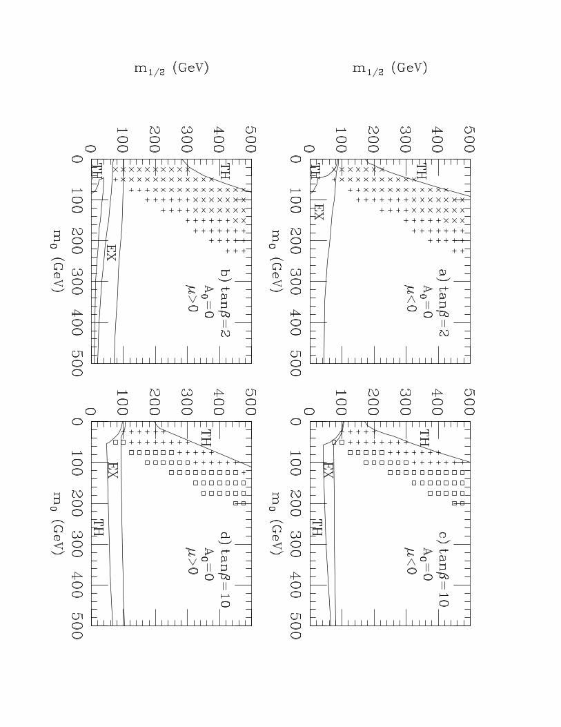
Using the procedures outlined in Sec. III and Appendices A and B, we explored regionsof minimal SUGRA parameter space for minima deeper than the standard MSSM one. Ourinitial scans took place in the m0 vs. m1/2 plane, to facilitate comparison with recent resultson fine-tuning, cosmology and present and future collider searches. We fix tan β(MZ) tobe 2 or 10, take A0 = 0 and mt = 170 GeV. Our search was performed in the ranges0 ≤ m0, m1/2 ≤ 500 GeV and the grid was scanned with 25 GeV resolution. Figures 6a-ddisplay the regions where non-standard global minima were discovered. Of all the directionsscanned for these plots, non-standard vacua were found only in the UFB-3a direction. InFig. 6, we have encoded information about the magnitude of the VEV in the plotting symbol.Using η = log10v/vMSSM, the squares represent 2 < η < 3, the crosses 3 < η < 4, andthe x’s 4 < η < 5. The most dangerous regions are those populated by squares: For thesepoints the “distance” between the standard and non-standard minima is smallest, whichwould admit the largest rate for tunnelling between them. Performing this scan using theexact prescription of Ref. [9] leads to nearly identical excluded regions.

We see from Fig. 6 that for all four frames, the region of low m0 becomes excluded.As noted in Ref. [9], this rules out the so-called “no-scale” models which require m0 = 0.In addition, in string models where supersymmetry is broken in the dilaton sector, one isled to GUT or string scale soft-terms related by m1/2 = −A0 =

√3m0 [22,23]. For this

precise choice of soft-term boundary conditions, much of the parameter space is excludedby non-standard minima. We further note that the excluded region rules out much of theSUGRA parameter space associated with light sleptons. In particular, taken literally, ourresults exclude regions where such decays as Z2 → ℓLℓ and Z2 → νν take place.

Although Fig. 6 is plotted for A0 = 0, a similar excluded region results for other choices ofthe A0 parameter. This is shown in Fig. 7, where we plot regions excluded in the m0 vs. A0

plane, for the same values of tanβ and µ, but for m1/2 fixed at 200 GeV. The vacuumconstraints exist for all A0 values, but are smallest for A0 ∼ 300 GeV.

9

In Fig. 8, we display a combined plot of Fig. 6 with superposed dark matter [10] and finetuning [11] contours. The regions to the right of the solid line contours are cosmologicallyexcluded because they predict a relic density Ωh2 > 1; this corresponds to a lifetime of theuniverse of less than 10 billion years. Cosmological models which take into account COBEdata, nucleosynthesis, and large-scale structure formation prefer an inflationary cosmology,with a matter content of the universe comprising 60% cold dark matter (e.g., neutralinos),30% hot dark matter (e.g., neutrinos), and 10% baryonic matter. In this case, the preferredrelic density of neutralinos should be .15 < Ωh2 < .4, i.e., the region between the dot-dashedcontours. In addition, Fig. 8 contains two naturalness contours with varying degrees ofacceptability: γ2 = 5 and 10 [11]. The more encompassing contour is a conservative estimateof a reasonable “tolerance limit” for weak scale supersymmetry. We see that the constraintfrom false vacua overlaps considerably with the preferred regions from cosmology and fine-tuning, leaving only a small preferred region of parameter space around m0 ∼ 100−200, andm1/2 ∼ 100 − 250 in each frame. We note that the resulting preferred region of parameterspace requires mg, mq, mW1

, mℓR

<∼ 650, 600, 220 and 175 GeV, respectively, for tanβ = 2,

and mg, mq, mW1, mℓR

<∼ 725, 650, 225 and 220 GeV for tan β = 10. The only exceptionto these bounds is if the neutralino is poised near the peak of an s-channel pole in itsannihilation cross section. These regions correspond to the narrow horizontal corridors inthe relic density contours.

Recently, the reach of the Fermilab Main Injector and TeV33 have been calculated in thesame parameter space frames [13]. By comparing the results of Ref. [13] with the preferredparameter space discussed above, we see that the TeV33 option covers most of the preferredregion from Fig. 8a via the clean trilepton signal from W1Z2 → 3ℓ, the exception beingthe region with m1/2

>∼ 180 GeV, where the spoiler decay mode Z2 → Z1h turns on. ForFig. 8b, TeV33 will cover the entire preferred region via clean trileptons. For the largetan β = 10 cases of Figs. 8c and d, the TeV33 upgrade can see most, but not all, of thepreferred parameter space regions. The reach of the Tevatron Main Injector is significantlyless than TeV33 for these preferred regions of parameter space. The CERN LHC collidercan of course probe all the preferred regions of parameter space. In fact, event rates willbe enormous for various multi-lepton + multi-jet +E/T channels, which should facilitateprecision measurements of parameters [14]. In particular, sleptons have mass less than 250GeV in these regions, and so ought to be visible at the LHC. Finally, we note that both thelight chargino and right-selectron have mass less than 250 GeV in the preferred regions, sothat both of these sparticles would be accessible to Next Linear Collider (NLC) experimentsoperating at

√s = 500 GeV [15].

V. CONCLUSION

The minimal SUGRA model provides a well-motivated and phenomenologically viablepicture of how weak scale supersymmetry might occur. The 4+1 dimensional parameterspace can be constrained in numerous ways as discussed in the introduction. To constrainthe model further, we have pursued the idea that parameter values that lead to globalminima in non-standard directions, such as those with charge or color breaking, should beexcluded from consideration. There are cosmological issues pertaining to tunnelling thatwe have knowingly ignored. Nevertheless, with this limitation noted, we searched for the

10

preferred regions of parameter space. We analyzed the potentials carefully employing the1-loop correction including the contributions of the top and stops in the calculation. Ingenerating the potential we found that the 1-loop correction can significantly alter resultsbased only on the tree approximation.

Because of the various scales present in the MSSM, renormalization group improvementhas ambiguities associated with it. We tried several procedures but were ultimately led totwo distinct results that we refer to as the α- and ω-cases. In the ω-case, to our surprise,the entire parameter space of the model suffers from global minima along non-standarddirections (namely the UFB-3(b) and CCB(a)-UP directions). Since the 2-loop correctionmay be significant, given the large value of the top mass, the results in the ω-case, whileintriguing, must be taken cum grano salis.

In the α-case, we are still left with a very restricted region of parameter space afterimposing in addition dark matter and naturalness constraints. Most of this region shouldbe accessible to the Fermilab TeV33 collider upgrade via the clean trilepton channel. Thisparameter space region should be entirely explorable at the LHC, and should yield a richharvest of multilepton signals for supersymmetry which ought to allow for precision deter-mination of underlying parameters. In addition, both charginos and sleptons ought to beaccessible to NLC experiments operating at just

√s = 500 GeV, so that the underlying

assumptions of the minimal SUGRA model can be well-tested.

ACKNOWLEDGMENTS

We thank Xerxes Tata and Greg Anderson for discussions. This research was supportedin part by the U. S. Department of Energy under grant number DE-FG-05-87ER40319.

11

APPENDIX A:

In this appendix, the cases from [9] that are considered in our investigation are reviewed.Also, formulas for the top/stops are displayed in each case and for the bottom/sbottoms inthe last case.• UFB-1: In the UFB-1 case, the only fields acquiring non-zero VEVs are < Φu >=<Φd >= x. The resulting tree level potential in this direction is

V =(m2

1 + m22 − 2|m2

3|)x2 , (A.1)

where m21 = m2

Φd+ µ2, m2

2 = m2Φu

+ µ2, and m23 = Bµ. The top mass is Mt = ytx, and the

stop mass matrix entries are

M2LL = m2

Q3+ y2

t x2 ,

M2RR = m2

u3+ y2

t x2 ,

M2LR = yt (µ − At) x . (A.2)

• UFB-2: In the UFB-2 case, an additional slepton field is included to help control theD-terms. The shifted fields are therefore

< Φu > = x ,

< Φd > = γx ,

< L3 >ν = γLx . (A.3)

The ν subscript represents the SU(2) direction that has acquired the VEV. The scalarpotential in this case is

V = γ2m21x

2 + m22x

2 − 2γ|m23|x2 + γ2

Lm2L3

x2 +1

4g2[1 − γ2 − γ2

L

]2x4 . (A.4)

Minimization with respect to γ and γ2L gives

γ =|m2

3|m2

1 − m2L3

, (A.5)

γ2L = 1 − γ2 − 2m2

L3

g2x2. (A.6)

If γ2L < 0, then γ2

L = 0, and we recover the UFB-1 direction. In this case, the top mass isMt = ytx, and the stop mass matrix entries are

M2LL = m2

Q3+ y2

t x2 +(

1

12g′2 − 1

4g22

) [1 − γ2 − γ2

L

]x2 , (A.7)

M2RR = m2

u3+ y2

t x2 − 1

3g′2[1 − γ2 − γ2

L

]x2 , (A.8)

M2LR = yt (µγ − At)x . (A.9)

• UFB-3(a): In the UFB-3(a) case, the shifted fields are

12

< Φu > = x ,

< Φd > = 0 ,

< L3 >2e = < e3 >2= ℓ2 = |µx

yτ

| ,

< L2 >ν = γLx . (A.10)

The VEVs of the (e3, e3) sleptons are fixed by imposing Φd F-term cancellation in thepotential. The scalar potential for this case is

V = m2Φu

x2 +(m2

L3+ m2

e3

)ℓ2 + γ2

Lm2L2

x2 +1

4g2[x2 + ℓ2 − γ2

Lx2]2

. (A.11)

Minimization with respect to γ2L gives

γ2L = 1 +

∣∣∣∣∣µ

yτx

∣∣∣∣∣−2m2

L2

g2x2. (A.12)

If γ2L < 0, then γ2

L = 0. In this case the top mass is Mt = ytx, and the stop mass matrixentries are

M2LL = m2

Q3+ y2

t x2 +(

1

12g′2 − 1

4g22

) [x2 + ℓ2 − γ2

Lx2]

, (A.13)

M2RR = m2

u3+ y2

t x2 − 1

3g′2[x2 + ℓ2 − γ2

Lx2]

, (A.14)

M2LR = −Atytx . (A.15)

• UFB-3(b): In the UFB-3(b) case, the shifted fields are

< Φu > = x ,

< Φd > = 0 ,

< Q3 >2d = < d3 >2= d2 = |µx

yb

| ,

< L3 >ν = γLx . (A.16)

The VEVs of the (d3, d3) squarks are fixed by imposing Φd F-term cancellation in thepotential. The scalar potential appears as

V = m2Φu

x2 +(m2

Q3+ m2

d3

)d2 + γ2

Lm2L3

x2 +1

4g2[x2 + d2 − γ2

Lx2]2

. (A.17)

Minimization with respect to γ2L gives

γ2L = 1 +

∣∣∣∣∣µ

ybx

∣∣∣∣∣−2m2

L3

g2x2. (A.18)

If γ2L < 0, then γ2

L = 0. In this case the top mass is Mt = ytx, and the stop mass matrixentries are

13

M2LL = m2

Q3+ y2

t x2 + y2b d2 +

1

12g′2[x2 + d2 − γ2

Lx2]− 1

4g22

[x2 − d2 − γ2

Lx2]

, (A.19)

M2RR = m2

u3+ y2

t x2 + y2t d2 − 1

3g′2[x2 + d2 − γ2

Lx2]

, (A.20)

M2LR = −Atytx . (A.21)

• CCB(a)-UP: In the CCB(a) case for the up-trilinear, the shifted fields are

< Φu > = x ,

< Φd > = 0 ,

< Q1 >u = αx ,

< u1 > = βx ,

< Q3 >2d = < d3 >2= d2 = |µx

yb

| ,

< L3 >ν = γLx . (A.22)

SU(3) D-flatness implies β2 = α2. Also, U(1) and SU(2) D-flatness imply 1 − α2 − γ2L = 0.

Consequently, the scalar potential appears as

V = y2u

(2 + α2

)α2x4 − 2T1α

2x2 +(M2α2 + m2

Φu+ m2

ℓ

)x2 , (A.23)

where T1 = |Auyux|, M2 = m2Q3

+ m2u3

− m2ℓ , and m2

ℓ = m2L3

. Minimization with respect toα2 yields

α2 =T1 − M2/2 − y2

ux2

y2ux

2. (A.24)

If α2 < 0, then α2 = 0 and γ2L = 1. If γ2

L < 0, then one should try < L3 >e=< e3 >= γLxand < L3 >ν= 0. D-flatness now implies 1−α2+γ2

L = 0. This also changes m2ℓ = m2

L3+m2

e3.

In this case the top mass is Mt = ytx, and the stop mass matrix entries are

M2LL = m2

Q3+ y2

t x2 + y2b d2 +

(1

12g′2 +

1

4g22

)d2 , (A.25)

M2RR = m2

u3+ y2

t x2 + y2t d2 − 1

3g′2d2 , (A.26)

M2LR = −Atytx . (A.27)

• CCB(b)-UP: In the CCB(b) case for the up-trilinear, the shifted fields are

< Φu > = x ,

< Φd > = γx ,

< Q1 >u = αx ,

< u1 > = βx ,

< L3 >ν = γLx . (A.28)

Unlike the previous CCB case (γ = 0), this case has three terms whose phases (ci = cos ϕi)are undetermined

14

2|Auyuu1ΦuQ1|c1 + 2|µyuu1Φ†dQ1|c2 + 2|µBΦuΦd|c3 . (A.29)

Reference [9] shows that this ambiguity can be resolved into two distinct possibilities. Ifsign(Au) = −sign(B), the three terms can be made simultaneously negative. If sign(Au) =sign(B), then the term of smallest magnitude is taken positive and the other two can betaken negative.

SU(3) D-flatness implies β2 = α2. Also, U(1) and SU(2) D-flatness imply 1 − α2 − γ2 −γ2

L = 0. Consequently, the scalar potential appears as

V = y2u

(2 + α2

)α2x4 + 2

(c1T1α

2 + c2T2α2|γ| + c3T3|γ|

)x2

+[M2α2 + (m2

1 − m2ℓ)γ

2 + m22 + m2

ℓ

]x2 , (A.30)

where

T1 = |Auyux| , (A.31)

T2 = |yuµx| , (A.32)

T3 = |µB| , (A.33)

M2 = m2Q3

+ m2u3

− m2ℓ , (A.34)

m21 = m2

Φd+ µ2 , (A.35)

m22 = m2

Φu+ µ2 , (A.36)

(A.37)

and where m2ℓ = m2

L3and ci = cos ϕi. Minimization with respect to α2 and |γ| (note that

the potential is a function of |γ|) yields

|γ| =c2T2α

2 + c3T3

m2ℓ − m2

1

, (A.38)

α2 = −y2ux

2 + M2/2 + c1T1 + c2T2|γ|y2

ux2

. (A.39)

It must be confirmed that both α2 > 0 and |γ| > 0. Otherwise these are set to zero. Itmust also be checked that γ2

L > 0. Otherwise one should try < L3 >e=< e3 >= γLx and< L3 >ν= 0. D-flatness now implies 1−α2−γ2+γ2

L = 0. This also changes m2ℓ = m2

L3+m2

e3.

In this case the top mass is Mt = ytx, and the stop mass matrix entries are

M2LL = m2

Q3+ y2

t x2 , (A.40)

M2RR = m2

u3+ y2

t x2 , (A.41)

M2LR = yt (µγ − At) x . (A.42)

• CCB(b)-TOP: In the CCB(b) case for the top-trilinear (there is no (a) case), the shiftedfields are

< Φu > = x ,

< Φd > = γx ,

< Q3 >u = αx ,

< u3 > = βx ,

< L3 >ν = γLx . (A.43)

15

SU(3) D-flatness implies β2 = α2. There is no imposition of D-flatness in the U(1) andSU(2) sectors. The potential now appears as

V = y2t

(2 + α2

)α2x4 +

[α2(m2

Q3+ m2

u3) + γ2m2

1 + γ2Lm2

L3+ m2

2

]x2

+ 2(c1T1α

2 + c2T2α2|γ| + c3T3|γ|

)x2 +

1

4g2(1 − α2 − γ2 − γ2

L

)x4 , (A.44)

where

T1 = |Atytx| , (A.45)

T2 = |ytµx| , (A.46)

T3 = |µB| , (A.47)

M2 = m2Q3

+ m2u3

− m2L3

, (A.48)

m21 = m2

Φd+ µ2 , (A.49)

m22 = m2

Φu+ µ2 . (A.50)

Minimization with respect to γ2L yields

γ2L = 1 − α2 − γ2 − 2m2

L3

g2x2. (A.51)

If γ2L > 0, then minimization with respect to α2 and |γ| gives

|γ| =c2T2α

2 + c3T3

m2L3

− m21

, (A.52)

α2 = −y2t x

2 + M2/2 + c1T1 + c2T2|γ|y2

t x2. (A.53)

If γ2L < 0, then it must be set to zero, and minimization with respect to α2 and |γ| yields

2y2t x

4(1 + α2

)− 1

2g2x4

(1 − α2 − γ2

)+(m2

Q3+ m2

u3

)x2 + 2 (c1T1 + c2T2|γ|)x2 = 0 (A.54)

−g2x4(1 − α2 − γ2

)|γ| + 2|γ|x2m2

1 + 2(c2T2α

2 + c3T3

)x2 = 0 . (A.55)

Substituting for |γ| yields a cubic equation for α2. It must still be checked that both |γ| > 0and α2 > 0. In this case the top mass is Mt = ytx, and the stop mass matrix entries are

M2LL = m2

Q3+ y2

t x2(1 + α2) +1

12g′2

[1 − 2

3α2 − γ2 − γ2

L

]x2

− 1

4g22

[1 − 3α2 − γ2 − γ2

L

]x2 +

1

3g23

[α2x2

], (A.56)

M2RR = m2

u3+ y2

t x2(1 + α2) − 1

3g′2

[1 − 7

3α2 − γ2 − γ2

L

]x2 +

1

3g23

[α2x2

], (A.57)

M2LR = yt (µγ − At) x +

[y2

t −1

3

(1

3g′2 + g2

3

)]x2αβ . (A.58)

• CCB(a)-ELECTRON: In the CCB(a) case for the electron-trilinear, the shifted fieldsare

16

< Φd > = x ,

< Φu > = 0 ,

< L1 >e = αx ,

< e1 > = βx ,

< Q3 >2u = < u3 >2= u2 = |µx

yt| . (A.59)

D-flatness implies α2 = β2 and α2x2 = x2 + u2. The scalar potential appears as

V = y2e

(2 + α2

)α2x4 +

[m2

Φd+ α2(m2

L1+ m2

e1)]x2 +

(m2

Q3+ m2

u3

)u2 − 2T1α

2x2 , (A.60)

where T1 = |Aeyex|. In this case we use the bottom/sbottom contribution. The bottommass is Mb = ybx, and the sbottom mass matrix entries are

M2LL = m2

Q3+ y2

bx2 +

(y2

t +1

2g22

)u2 , (A.61)

M2RR = m2

d3+ y2

b

(x2 + u2

), (A.62)

M2LR = Abybx . (A.63)

• CCB(b)-ELECTRON: In the CCB(b) case for the electron-trilinear, the shifted fieldsare

< Φd > = x ,

< Φu > = γx ,

< L1 >e = αx ,

< e1 > = βx . (A.64)

D-flatness again implies β2 = α2 and α2 = 1 − γ2. The potential appears as

V = y2e

(2 + α2

)α2x4 +

[m2

1 + γ2m22 + α2(m2

L1+ me1

2)]x2

+ 2(c1T1α

2 + c2T2α2|γ| + c3T3|γ|

)x2 , (A.65)

where

T1 = |Aeyex| , (A.66)

T2 = |yeµx| , (A.67)

T3 = |µB| . (A.68)

Substituting for α2 and minimizing with respect to |γ| gives the following cubic equation

|γ|3[2y2

ex2]− γ2 [3c2T2] + |γ|

[(m2

2 − m2L1

− m2e1

)− 4y2

ex2 − 2c1T1

]+ [c2T2 + c3T3] = 0 .

(A.69)

It must be checked that both |γ| > 0 and α2 > 0. In this case the top mass is Mt = γytx,and the stop mass matrix entries are

17

M2LL = m2

Q3+ γ2y2

t x2 , (A.70)

M2RR = m2

u3+ γ2y2

t x2 , (A.71)

M2LR = yt (µ − γAt)x . (A.72)

If γ = 0, then we use the bottom/sbottom contribution. The bottom mass is Mb = ybx, andthe sbottom mass matrix entries are

M2LL = m2

Q3+ y2

b x2 , (A.73)

M2RR = m2

d3+ y2

b x2 , (A.74)

M2LR = Abybx . (A.75)

18

APPENDIX B:

We find that Eq. (2.3) cannot be reliably calculated using our computer for large (>106) values of the VEVs. We therefore use a limiting form of this expression in the largeVEV limit. This limiting form of ∆V1 is presented in this appendix. We begin with somedefinitions:

mt = ytx (B.1)

M2LL = m2

t + m2L + MLx + GLx2 (B.2)

M2RR = m2

t + m2R + MRx + GRx2 (B.3)

M2LR = Mx + Gx2 . (B.4)

These expressions cover all the cases we have analyzed, and it is a simple matter to identifythe various coefficients for each case. Note that in the CCB-ELECTRON cases, mt shouldbe substituted with mb. In terms of these definitions, the two stop masses are

M2

t±=

1

2

[2m2

t + (m2L + m2

R) + (ML + MR)x + (GL + GR)x2]

±[

(m2L − m2

R) + (ML − MR) + (GL − GR)x2]2

+ 4[Mx + Gx2

]21/2

. (B.5)

To simpifly the notation some new definitions are used, and the stop masses rewritten interms of these

M2

t±= m2

t

[1 +

(G+

2y2t

)+

1

mt

(M+

2yt

)+

1

m2t

(m2

+

2

)]

± 1

2m2

t

[α2 +

1

mtβ2 +

1

m2t

γ2 +1

m3t

δ2 +1

m4t

ǫ2

]1/2

(B.6)

where

G± = GL ± GR (B.7)

M± = ML ± MR (B.8)

m2± = m2

L ± m2R (B.9)

α2 = (G2− + 4G2)/y4

t (B.10)

β2 = 2(G−M− + 4MG)/y3t (B.11)

γ2 = (M2− + 2m2

−G− + 4M2)/y2t (B.12)

δ2 = 2m2−M−/yt (B.13)

ǫ2 = m4− . (B.14)

Modulo overall factors the 1-loop correction is

∆V1 = −2m4t lnm2

t/Q2 + M4

t+lnM2

t+/Q2 + M4

t−lnM2

t−/Q2 (B.15)

where Q = Qe3/4. There are three cases to be considered• case (a): α2 6= 0,

19

A± = 1 +G+

2yt

± α

2(B.16)

B± =M+

2yt± β2

4α(B.17)

C± =m2

+

2± 4α2γ2 − β4

16α3(B.18)

• case (b): α2 = 0 (=> β2 = 0); γ2 6= 0,

A± = 1 +G+

2yt

(B.19)

B± =M+

2yt± γ

2(B.20)

C± =m2

+

2± δ2

4γ(B.21)

• case (c): α2 = β2 = γ2 = δ2 = 0; ǫ2 6= 0,

A± = 1 +G+

2yt

(B.22)

B± =M+

2yt(B.23)

C± =m2

+

2± ǫ

2(B.24)

Finally the form of the 1-loop correction in the large mt limit is

∆V1 = m4t[2(a+ + a−) + (a2

+ + a2−)]L +

(A2

+ lnA+ + A2− lnA−

)

+2

mt[A+B+(1/2 + L + ln A+) + A−B−(1/2 + L + ln A−)]

+1

m2t

[B2+(3/2 + L + ln A+) + B2

−(3/2 + L + ln A−)

+ 2A+C+(1/2 + L + ln A+) + 2A−C−(1/2 + L + ln A−)] (B.25)

where L = lnm2t/Q

2 and a± = A± − 1. To arrive at ∆V1, multiply the above expressionby 3/32π2.

20

REFERENCES

[1] H. Haber, Lectures presented at TASI-92, University of Colorado, Boulder, (hep-ph/9306207); X. Tata, in The Standard Model and Beyond, p. 304, edited by J. E. Kim,World Scientific (1991).

[2] A. Chamseddine, R. Arnowitt and P. Nath, Phys. Rev. Lett. 49, 970 (1982); R. Barbieri,S. Ferrara and C. Savoy, Phys. Lett. B119, 343 (1982); L. Hall, J. Lykken and S.Weinberg, Phys. Rev. D27, 2359 (1983); P. Nath, R. Arnowitt and A. Chamseddine,Nucl. Phys. B227, 121 (1983).

[3] L. Ibanez and G. Ross, Phys. Lett. 110B, 215 (1982); K. Inoue, A. Kakuto, H. Komatsuand S. Takeshita, Progr. Theor. Phys. 68, 927 (1982); L. Alvarez-Gaume, M. Claudsonand M. Wise, Nucl. Phys. B207, 96 (1982); J. Ellis, D. Nanopoulos and K. Tamvakis,Phys. Lett. B121, 123 (1983).

[4] H. Haber, in Properties of SUSY Particles, L. Cifarelli and V. Khoze, Editors, WorldScientific (1993).

[5] For a recent review, see G. Jungman, M. Kamionkowski and K. Griest, Phys. Rep. 267,195 (1996); see also J. Ellis, CERN-TH.7083/93 (1993).

[6] H. Baer, C. H. Chen, R. Munroe, F. Paige and X. Tata, Phys. Rev. D51, 1046 (1995).[7] J. M. Frere, D. R. T. Jones and S. Raby, Nucl. Phys. B222, 11 (1983); L. Alvarez-

Gaume, M. Claudson and M. Wise, Nucl. Phys. B221, 495 (1984); J. P. Derendingerand C. Savoy, Nucl. Phys. B237, 307 (1984); C. Kounnas, A. B. Lahanas, D. Nanopoulosand M. Quiros, Nucl. Phys. B236, 438 (1984); M. Claudson, L. Hall and I. Hinchliffe,Nucl. Phys. B228, 501 (1983); M. Drees, M. Gluck and K. Grassie, Phys. Lett. B157,164 (1985); J. Gunion, H. Haber and M. Sher, Nucl. Phys. B306, 1 (1988); H. Komatsu,Phys. Lett. B215, 323 (1988).

[8] G. Gamberini, G. Ridolfi and F. Zwirner, Nucl. Phys. B331, 331 (1990).[9] J.A. Casas, A. Lleyda, and C. Munoz, FTUAM-95-11 (Jun. 1995), hep-ph/9507294.

[10] H. Baer and M. Brhlik, Phys. Rev. D53, 597 (1996).[11] G.W. Anderson and D.J. Castano, Phys. Rev. D53, 2403 (1996).[12] H. Baer, M. Brhlik, R. Munroe and X. Tata, Phys. Rev. D52, 5031 (1995).[13] H. Baer, C. H. Chen, C. Kao and X. Tata, Phys. Rev. D52, 1565 (1995); H. Baer, C.

H. Chen, F. Paige and X. Tata, FSU-HEP-960415 (1996), hep-ph/9604406.[14] H. Baer, C. H. Chen, F. Paige and X. Tata, Phys. Rev. D52, 2746 (1995) and Phys.

Rev. D53, 6241 (1996).[15] T. Tsukamoto, K. Fujii, H. Murayama, M. Yamaguchi and Y. Okada, Phys. Rev.

D51, 3153 (1995); H. Baer, R. Munroe and X. Tata, FSU-HEP-960601 (1996), hep-ph/9606325.

[16] A. Kusenko, P. Langacker and G. Segre, UPR-0677-T (Feb. 1996), hep-ph/9602414.[17] A. Strumia, FTUAM-96-14 (Apr. 1996), hep-ph/9604417.[18] G. W. Anderson, private communication.[19] See, for example, M. Sher, Phys. Reps. 179, 273 (1989).[20] B. de Carlos and J. A. Casas, Phys. Lett. B309, 320 (1993).[21] D. J. Castano, E. J. Piard, and P. Ramond, Phys. Rev. D49, 4882 (1994).[22] V.S. Kaplunovsky and J. Louis, Phys. Lett. B306, 269 (1993).[23] A. Brignole, L.E. Ibanez, and C. Munoz, Nuc. Phys. B422, 125 (1994).

21

FIGURES

FIG. 1. Plots of the 1-loop correction, tree and 1-loop effective potentials along the MSSM and

UFB-3(a) vacuum directions in the A0 = 0, m0 = 100 GeV, m1/2 = 200 GeV, µ < 0, and tan β = 2

case. Renormalization group improvement was implemented using the α- prescription.

FIG. 2. Plots similar to Fig. 1 but with renormalization group improvement implemented using

the ω-prescription.

FIG. 3. Plots of the logarithm of the VEV versus χ, a parameter appearing in the renormal-

ization group improvement function, for the vacuum directions UFB-3(b) and CCB(a)-UP.

FIG. 4. Evolution of the VEV by using the renormalization group γ functions of the Higgs

fields (solid line) and by tracking the minimum of 1-loop potential (dashed line) as a function of

the renormalization scale Q.

FIG. 5. Plots of the potential in the CCB(a)-UP case. In (a) the tree potential is displayed. In

(b) the 1-loop potential is displayed for both α and ω precriptions.

FIG. 6. Exclusion plots for the m0 vs. m1/2 plane based on the UFB-3(a) constraint. The

squares represent 2 < η < 3, the crosses 3 < η < 4, and the x’s 4 < η < 5.

FIG. 7. Exclusion plots for the m0 vs. A0 plane based on the UFB-3(a) constraint and with

m1/2 = 200 GeV. The symbols are the same as in Fig. 6.

FIG. 8. Same as Fig. 6 but with superposed dark matter (dot dashes and solid) and naturalness

(dashes) contours.

22