arX

iv:0

705.

1499

v2 [

hep-

ph]

28

Sep

2007

IISc-CHEP/06/07

LAPTH-1183/2007

Top production at the Tevatron/LHC and nonstandard, stronglyinteracting spin one particles

Debajyoti Choudhurya, Rohini M. Godboleb,c, Ritesh K. Singhd and Kshitij Waghe

aDept. of Physics and Astrophysics, University of Delhi, Delhi 110 007, India.

bCentre for High Energy Physics, Indian Institute of Science, Bangalore, 560 012, India.

c Dept. of Theoretical Physics, Tata Institute of Fundamental Research,

Mumbai 400 005, India.

d Laboratoire d’Annecy-Le-Vieux de Physique Theorique (LAPTH), Chemin de Bellevue, B.P. 110,

F-74941 Annecy-le-Vieux, Cedex, France.

e Dept. of Physics and Astronomy, Rutgers University, Piscataway,

New Jersey 08854-8019, U.S.A.

Abstract

In this note, we consider possible constraints from tt production on the gauge bosons oftheories with an extended strong interaction sector such as axigluons or flavour universalcolorons. Such constraints are found to be competitive with those obtained from thedijet data. The current tt data from the Tevatron rule out axigluon masses (mA) upto 910 GeV and 920 GeV at 95% and 90% confidence levels respectively. For the caseof the flavour universal colorons, for cot ξ = 1, where ξ is the mixing angle, the massranges mC

<∼ 800 GeV and 895 <∼ mC<∼ 1960 GeV are excluded at 95% confidence

level (C.L.), whereas the same at 90% C.L. are mC <∼ 805 GeV and 880 <∼ mC <∼ 2470GeV. For cot ξ = 2 on the other hand, the excluded range is mC

<∼ 955(960) GeV and1030 <∼ mC <∼ 3250 (1020 <∼ mC <∼ 3250) GeV at 95%(90%) C.L. respectively. We pointout that for higher axigluon/coloron masses, even for the dijet channel, the limits on thecoloron mass, for cot ξ = 1, may be different than those for the axigluon. We also computethe expected forward-backward asymmetry for the case of the axigluons which would allowit to be discriminated against the SM as also the colorons. We further find that at theLHC, the signal should be visible in the tt invariant mass spectrum for a wide range ofaxigluon and coloron masses that are still allowed. We point out how top polarisation maybe used to further discriminate the axigluon and coloron case from the SM as well as fromeach other.

1 Introduction

The Standard Model (SM) has had unprecedented success in passing precision tests at the SLC, LEP,

HERA and the Tevatron. The agreement between the directly measured value of the top mass, mt,

and the one indicated by precision measurements [1, 2], has played a crucial role in this test of the

SM to the loop level, providing indirect evidence for the Higgs boson. However, a direct verification

of the Higgs mechanism of the spontaneous breaking of the Electroweak (EW) symmetry, thereby

providing an understanding of the mechanism of the mass generation for fermions, is still lacking.

Its understanding will be one of the focal points of the investigations at the Large Hadron Collider

(LHC) and, thereafter, the International Linear Collider(ILC) [3]. The top quark, with a mass very

close to the electroweak symmetry breaking scale, is expected to provide a probe for understanding

the phenomenon of symmetry breaking in the SM. For the same reason, any alternative to the Higgs

mechanism almost always involves the top quark [4]. Thus, a study of production and properties of

the top quark at the TeV colliders can be used as a ‘low’ energy probe for any (‘high scale’) new

physics beyond the SM, as well as a good probe of alternates to the Higgs mechanism. An accurate

testing of the mass relations between mt and mW , as predicted in the SM, is an important part of

the physics program of any TeV energy collider [5]. Clearly, top physics is a very promising place

to look for new physics effects [6]. Already at the Tevatron, this has been a very fruitful area of

investigations [7, 8] and one expects a top factory such as the LHC to be a goldmine for studying

the SM as well as the beyond the SM(BSM) physics [9]. Recent discussions in the literature have

addressed the possibility of using tt production at the Tevatron for putting ‘direct’ constraints [10] on

the Kaluza Klein(KK) gluons of the bulk Randall-Sundrum Model, using their large coupling to the tt

pairs to probe the same at the LHC through use of t polarisation, in tt production [11, 12], as well as

using spin-spin correlations in tt production via KK excitations of the graviton [13]. tt pair production

at the Tevatron through a Z ′t in various versions of Topcolor models has also been discussed [14]. The

feasibility of using the t polarisation in tt production via an EW resonance such as an additional

Z ′ occurring in (say) unified models or a ZH which occurs in the Little Higgs models has also been

recently explored [15]. In this note, we revisit the issue of constraints that the current measurements of

tt production at the Tevatron [7, 8] imply for theories which have a strongly interacting spin-1 particle

in addition to the gluons. We discuss the tt production for the cases of massive coloured ‘axigluons’

which exist in theories with chiral colour [16, 17] and that of the flavour universal colorons [18] which

exist in certain versions of extended colour gauge theories. It may be mentioned here that the case of

axigluons and the flavour universal colorons differs from the other strongly interacting bosons such as

the KK gluons or the ETC theories, in that they do not have preferential coupling to tt. Thus, the

sensitivity of tt production to our case should be expected to differ from that for such models with

enhanced top-couplings.

Below, we first summarise the relevant details of the two models as well as the current limits on

the masses of the axigluons and flavour universal colorons. Then we will show the constraints the

1

current data on tt production imply for these. We then look at the phenomenology of the colorons

and the axigluons at the LHC as well.

2 Models.

In the unifiable chiral colour model [16, 17], the high energy strong interaction gauge group SU(3)L ×SU(3)R is spontaneously broken to the usual SU(3)L+R and thus one has an octet each of massless

gluons(g) and massive axigluons (A) with an axial vector coupling, 12gsγµγ5λ

a, where gs is the usual

strong coupling and λa the usual Gell-Mann matrices. The above mentioned axigluon is common to

all the different versions of the chiral colour models that exist. The strong coupling of A to qq ensures

large production cross-sections for the axigluons at a hadronic collider, at the same time causing the

axigluon to have a reasonably large width. Considerations of embedding the chiral colour group into a

grand unified theory implied a ‘natural’ value for the axigluon mass of the order of the weak scale ∼ 250

GeV. It was soon realised that not only could the axigluon be searched for in the dijet channel [19]

through the process pp(p) → A∗ → qq, but also that the forward-backward asymmetry caused by

the interference between the g and A contributions to qq → QQ [20] could be used to probe and

constrain the A contribution. The Tevatron searches for new resonances decaying to dijets [21, 22]

exclude the mass range 200 < mA < 1130 GeV. The lighter axigluon windows were eliminated by

various considerations such as hadronic decays of the Z-boson etc. [23, 24]. tt production through

the process qq → tt can be used very effectively for the axigluon search due to large qq fluxes at the

Tevatron. The large top-sample at the Tevatron was shown capable of providing reach of the order

of 1 TeV for generic new physics [6]. The early Tevatron data on top-pair production was shown [25]

to disfavour the contribution from a lighter axigluon mass window 50 < mA < 120 GeV (which was

then not completely ruled out) at about 1.5σ level. The analysis can be further sharpened by using

the forward-backward asymmetry in the tt production.

The flavour universal coloron model [18] belongs to a class of models of extended colour which

arose from the general effort to understand the mechanism of EW symmetry breaking and the large

mass of the top, mt, in the same framework, and wherein a top quark condensate enhances the top

quark mass and drives the EW symmetry breaking. Specific examples of this idea are topcolor [26, 6]

and topcolor assisted technicolor [27]. In general, in the coloron models, it is assumed that the colour

group at high energies is larger, given by SU(3)I × SU(3)II , and breaks at the TeV scale to the usual

SU(3)c, giving rise to an octet of massive, strongly interacting gauge bosons, called colorons. Variants

of the coloron models differ in how the different generations of quarks couple to SU(3)I and SU(3)II .

In the original model [26, 6], the first two families couple to SU(3)I and the third couples to SU(3)II .

The phenomenology of such a coloron at the Tevatron and at the LHC, with respect to the tt final

states has been discussed [6, 28]. The Universal flavour coloron model [18, 29], is a variant of this

idea, where all the quarks transform as a (1, 3) under this extended gauge group and the two gauge

couplings are ξ1, ξ2 for SU(3)I and SU(3)II respectively, with ξ1 ≪ ξ2. The massive colorons couple

2

to all the quarks through a 12gs cot ξγµλa coupling, where ξ is the mixing angle given by cot ξ = ξ2/ξ1.

The mass of the coloron mC is related to ξ, the strong coupling gs and the vacuum expectation value

of the scalar Φ which transforms as a (3, 3) under the extended gauge group and breaks it down to

SU(3)c. The coloron, like the axigluon, is also a broad resonance. The model with flavour universal

coloron can be grafted rather nicely onto the standard one-Higgs-doublet model of EW physics and

has a naturally heavy top quark [30]. Electroweak precision measurements constrain the ρ parameter

and hence the model parameter space, the constraint being given by Mc/ cot ξ >∼ 450 GeV [31] 1.

Further, the value of cot ξ is limited from above to ∼ 4, by the requirement that the model remains

in the Higgs phase.

The colorons will contribute to the dijet production [29, 32] in almost the same way as the axiglu-

ons. The constraints on mA from the dijet data [21, 22] can also be translated into constraints on mC .

However, the coloron contribution will not give rise to any forward-backward asymmetry in qq produc-

tion as opposed to the case of the axigluons. Ref. [29] estimated the possible constraints that may be

obtained with the b–tagged dijets, using the analysis constraining the topgluon production and decay,

accounting for the difference in the possible decay channels and the width in the two cases. Further,

it was claimed [29] that while using the approximation of incoherent sum of the background and the

signal, the signal strengths in the dijet channel for the flavour universal coloron for cot ξ = 1 will be

the same as that of an axigluon of the same mass. It was further claimed [29], that since the expected

cross-sections for the coloron, in the above approximation, increase with cot ξ, the constraints implied

by the dijet analysis for the axigluons also give the most conservative constraint for the coloron. At

present, the best quoted bounds for axigluon and colorons come from the Tevatron dijet data which

rule out masses up to ≃ 980 GeV [22, 24]. As we point out later, for heavier coloron masses, some of

the above statements need to be amended.

3 Axigluon and Coloron contribution to tt production at hadronic

colliders.

At the tree level, the presence of an axigluon A or the coloron C can affect tt production only as far

as the qq-initiated subprocess is concerned, leaving the gg-initiated subprocess unaltered. Since the

qq fluxes are dominant over the gg fluxes at the Tevatron, the possible presence of a axigluon/coloron

resonance (the s-channel qq → A∗(C∗) → tt diagram is the only new contribution) can affect the total

rate of tt production significantly. This can be easily understood by realising that, at the Tevatron,

even in the absence of these exotic bosons (i.e., even for the SM alone), the contribution to the total

tt cross-section from the qq initial state dominates over the gg contribution by a factor of ∼ O(10),

depending on the PDF’s, choice of scale etc.

In the presence of an axigluon, the parton-level differential cross section for the qq-initiated process

1We have checked that current precision measurements also imply a similar constraint.

3

is modified and for final state t(t) with helicity λ(λ) is given by,

dσ

dt(qq → t(λ)t(λ)) =

π α2s

9 s2

{[

(1 + λ λ)4m2

t

s(1 − c2

θ) + (1 − λ λ) (1 + c2θ)

]

+(1 − λ λ)

(s − m2A)2 + Γ2

A m2A

[

s2 β2 (1 + c2θ) + 4 s (s − m2

A) β cθ

]

}

,

(1)

where s is the invariant mass of the tt system with β(≡√

1 − 4m2t /s) and θ being the top-velocity and

the scattering angle in the parton centre of mass frame respectively; λ and λ which are the helicities

(as distinct from chirality) of the top and the anti-top, and take values ±1. Note that there are no

terms linear in the helicities, as would have been present if the intermediate boson (axigluon) were to

have both vectorial and axial couplings. The width ΓA is given by

ΓA ≡∑

q

Γ(A → qq) ≈ αs mA

6

[

5 +

(

1 − 4m2t

m2A

)3/2]

. (2)

Summing over the top polarizations, the expression for the cross-section for tt production for the qq

initial state becomes,

dσ

dt(qq → tt) =

2π α2s

9 s2

{[

4m2t

s(1 − c2

θ) + (1 + c2θ)

]

+s2 β2 (1 + c2

θ) + 4 s (s − m2A) β cθ

(s − m2A)2 + Γ2

A m2A

}

,

(3)

and reduces to Eq. [2.2] of [19] in the limit of zero quark (top) mass. Note the existence of the term

odd in cθ here, which is due to the interference between the gluon and the axigluon amplitude. We

may mention here that our Eq. 3 does not agree with Eq.[2] of Ref. [20]. The interference term in

their Eq. [2] is proportional to β2 instead of β as in our Eq. 3; further as per their Eq.[2] the square

of the axigluon exchange amplitude is proportional to the gluon exchange amplitude, apart from the

obviously different propagator, which can not be true for massive quarks in the final state. Needless to

mention of course that the first term in eq. 3, corresponding to the SM, agrees with the standard QCD

expression [33], now available in textbooks on the subject. Since the contribution of the gg initial

state [33] (to be added incoherently) remains unchanged we refrain from reproducing the formulae

here.

In the presence of the coloron, the differential cross-section for production of production of t(t)

with helicities λ(λ) respectively, reads for the qq initial state:

dσ

dt(qq → t(λ)t(λ)) =

π α2s

9 s2

{

(1 + λ λ)4m2

t

s(1 − c2

θ) + (1 − λ λ) (1 + c2θ)

}

∣

∣

∣

∣

1 +s cot2 ξ

s − m2C + iΓC mC

∣

∣

∣

∣

2

.

(4)

4

The width is now given by

ΓC ≡∑

q

Γ(C → qq) =αs cot2 ξ

6mC

{

5 +

[

1 + 2m2

t

m2C

] (

1 − 4m2t

m2C

)1/2}

. (5)

Once again, summing over the polarization gives us for the differential cross-section

dσ

dt(qq → tt) =

2π α2s

9 s2

{

4m2t

s(1 − c2

θ) + (1 + c2θ)

}

∣

∣

∣

∣

1 +s cot2 ξ

s − m2C + iΓC mC

∣

∣

∣

∣

2

. (6)

As far as the coloron is concerned, the net effect of the addition of a simple vectorial interaction is to

just change the propagator from 1/s to 1/s + cot2 ξ/(s−m2C + imCΓC) [6], in the qq → tt amplitude.

Our Eq. 6 agrees with Eq.[3.7] of Ref. [29] and also with Eq.[3.3], the corresponding expression for

dijet cross-section, when the limit of zero top mass is taken. In the absence of the coloron contribution

the term in Eq. 6 proportional to cot ξ is absent and then the expression trivially reduces to the usual

QCD contribution for the qq initial state [33]. Again the presence of colorons does not modify the

contribution of the gg initial state from its SM form.

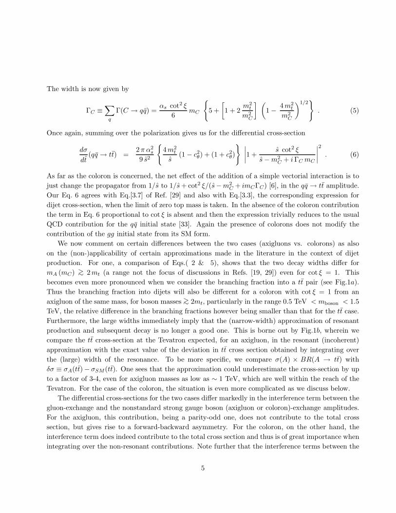
We now comment on certain differences between the two cases (axigluons vs. colorons) as also

on the (non-)applicability of certain approximations made in the literature in the context of dijet

production. For one, a comparison of Eqs.( 2 & 5), shows that the two decay widths differ for

mA (mC) >∼ 2mt (a range not the focus of discussions in Refs. [19, 29]) even for cot ξ = 1. This

becomes even more pronounced when we consider the branching fraction into a tt pair (see Fig.1a).

Thus the branching fraction into dijets will also be different for a coloron with cot ξ = 1 from an

axigluon of the same mass, for boson masses >∼ 2mt, particularly in the range 0.5 TeV < mboson < 1.5

TeV, the relative difference in the branching fractions however being smaller than that for the tt case.

Furthermore, the large widths immediately imply that the (narrow-width) approximation of resonant

production and subsequent decay is no longer a good one. This is borne out by Fig.1b, wherein we

compare the tt cross-section at the Tevatron expected, for an axigluon, in the resonant (incoherent)

approximation with the exact value of the deviation in tt cross section obtained by integrating over

the (large) width of the resonance. To be more specific, we compare σ(A) × BR(A → tt) with

δσ ≡ σA(tt)− σSM (tt). One sees that the approximation could underestimate the cross-section by up

to a factor of 3-4, even for axigluon masses as low as ∼ 1 TeV, which are well within the reach of the

Tevatron. For the case of the coloron, the situation is even more complicated as we discuss below.

The differential cross-sections for the two cases differ markedly in the interference term between the

gluon-exchange and the nonstandard strong gauge boson (axigluon or coloron)-exchange amplitudes.

For the axigluon, this contribution, being a parity-odd one, does not contribute to the total cross

section, but gives rise to a forward-backward asymmetry. For the coloron, on the other hand, the

interference term does indeed contribute to the total cross section and thus is of great importance when

integrating over the non-resonant contributions. Note further that the interference terms between the

5

0

0.02

0.04

0.06

0.08

0.1

0.12

0.14

0.16

0.18

0.4 0.8 1.2 1.6 2.0

Br

(tt)

m (TeV)

(a)Axigluon

Coloron

10−3

10−2

10−1

1

10

102

0.4 0.8 1.2 1.6 2.0 2.4

σ tt [

pb]

m (TeV)

√s = 1.96 TeV

CTEQ-6L1

(b)

δσ(tt, offshell A)

σ(A) × Br(A → tt)

Figure 1: (a) The branching fraction of axigluon/coloron to a tt pair as a function of the boson mass;

(b) A comparison of the deviation of the total tt cross section caused by the presence of an axigluon

(solid line) with the resonant production followed by decay.

coloron and gluon-exchange contributions changes sign as the subprocess centre of mass energy√

s

passes through mC , and, depending on the value of cot ξ, can even reduce the total integrated cross-

section below the SM value. Thus, the interference term has different behaviour for the coloron and

the axigluon. As can be also seen from Eqs. 3 and 6, even the term in the cross-section proportional

to the square of the propagator of the unstable strong boson (axigluon or coloron) is different in the

two cases for massive quarks in the final state.

The observations above have several implications. First, it is clear that for mA,mC <∼ 1.5 TeV,

as far as the tt production cross-section is concerned, (even on resonance) the expectations for a

coloron with cot ξ = 1 will be different from that for an axigluon of the same mass, unlike the case of

dijet cross-sections where only massless quarks are involved. Even for the latter case, for the heavier

colorons now being looked for in the Tevatron dijet data, for cot ξ = 1, the σ × B , is no longer the

same as that of an axigluon of the same mass. As was already mentioned, an equality between these,

claimed in Ref. [29] and used in all the analyses [22, 24] so far, is true only for relatively low values of

the boson masses. It may be pointed that even in that case the (approximate) equality is true only

when the resonant contribution dominates and one considers only the incoherent sum of background

and the signal. With increasing mass of the boson, the width increases, necessitating the inclusion

of the interference term to the total cross-section and the approximation of incoherent sum of the

background and the signal is no longer valid. For the case of the colorons, the effect of the parity-even

interference term gives a non monotonic dependence of the total integrated cross-section on mC and

cot ξ. Thus it means that for heavier colorons, a value of mass mC excluded at cot ξ = 1 need not be

6

excluded at higher values of cot ξ.

4 Numerical Results and constraints from tt production at Tevatron

Using the formulae presented in section 3 (and including the contribution from the gg initial state [33]),

we now proceed to calculate the tt cross-section at the Tevatron Run II (√

s = 1.96) and assess the

implications of the current data. For all our computations, we use the CTEQ-6L1 parton distribu-

tions [34], with a choice of Q2 = m2t for the factorization scale and mt = 175 GeV. For the SM process,

corresponding K–factor corresponding to this choice of PDF and the scale, amounts to 1.08 [35]. As

mentioned earlier, at the Tevatron, the SM production process is dominated by the qq initial states,

and since both the color and tensorial structure of the process under consideration is very similar to

the SM process, it is expected that the use of the SM K-factor for the cross-section including the

effects of the axigluon/coloron contribution is well justified. This is what we shall use henceforth.

We have verified that except very close to the peaks, the cross-sections are stable with respect to a

change in the scale of the hard process (and/or the choice of the parton distributions) as long as the

corresponding correct K-factor [35] is used. While the smallness of K(1.08) for our choice of parton

density, is a reflection of the rather large value of αs(MZ) = 0.130 used in CTEQ-6L1, note that this

choice of parton densities is not a special one.

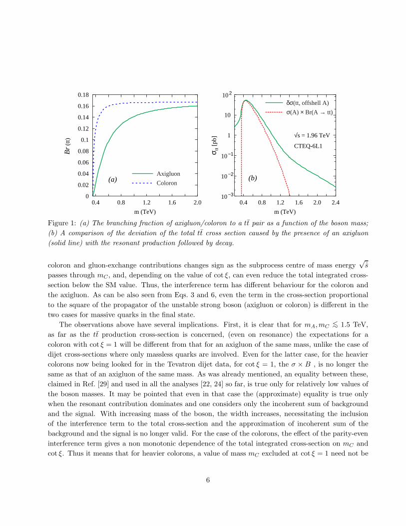
In Fig.2, the solid (green) line shows our predictions for the tt production cross-section as a function

of the axigluon mass. This may be compared with the current experimental data which gives (CDF

Run II results averaged over all channels) [7]

σ(p + p → t + t + X;√

s = 1.96TeV) = 7.3 ± 0.5 (stat) ± 0.6 (syst) ± 0.4 (lum) pb . (7)

In Fig.2, the central value is denoted by the horizontal grey dashed line, whereas the sidebands (dashed

black and magenta lines respectively) give the 95% –Confidence Level (C.L.) limits (obtained by adding

the errors in quadrature). As can be seen from the plot, the data rule out axigluon masses(mA) up to

910 GeV at 95% C.L. It can be easily seen that these are comparable to the current constraints [22, 24]

available from the Tevatron dijet data. As already mentioned before, predictions for the tt production

for the coloron (even for cot ξ = 1) differ from that for the axigluon of the same mass. In particular,

due to the destructive (parity-even) interference for s < m2C , the cross-section shows a dip as a function

of mC and rises again. That the extent of this interference depends crucially on the magnitude of cot ξ

can be understood from the discussion following Eq.(6). As can be clearly seen, in this case, the data

rule out values of mC below 800 GeV at 95% confidence level and also the mass range between 895

GeV to 1960 GeV at 95% confidence level, for cot ξ = 1. At 90% C.L. the exclusion is for mC < 805

GeV and for masses between 880 GeV to 2470 GeV. For cot ξ = 2 on the other hand, the excluded

range at 95% C.L. is mC <∼ 955 GeV and 1030 <∼ mC <∼ 3250 GeV. At 99.99% C.L., the same is, e.g.,

mC <∼ 930 GeV and 1110 <∼ mC <∼ 1860 GeV.

7

1

10

100

1000

0.4 0.8 1.2 1.6 2.0 2.4

σ tt [fb]

mBoson (TeV)

√s = 1.96 TeV

CTEQ-6L1

Axigluon

Coloron : cot ξ = 1

Coloron : cot ξ = 2

Figure 2: tt production cross-section at the Tevatron as a function of the axigluon (coloron mass)

and constraints on it from the current tt production data. The solid (green) line corresponds to the

axigluon case. The short- (blue) and long-dashed (red) lines correspond to the flavour universal coloron

for cot ξ = 1 and cot ξ = 2 respectively. The horizontal lines correspond to the current central value

from the CDF experiment [7] and the 95% confidence level bands. We have used CTEQ-6L1 parton

distribution functions evaluated at Q = mt and included the appropriate K–factor [35].

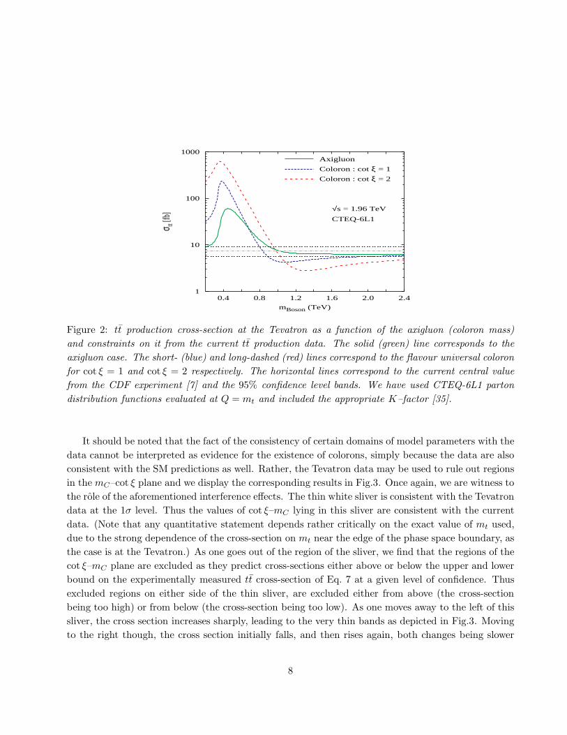
It should be noted that the fact of the consistency of certain domains of model parameters with the

data cannot be interpreted as evidence for the existence of colorons, simply because the data are also

consistent with the SM predictions as well. Rather, the Tevatron data may be used to rule out regions

in the mC–cot ξ plane and we display the corresponding results in Fig.3. Once again, we are witness to

the role of the aforementioned interference effects. The thin white sliver is consistent with the Tevatron

data at the 1σ level. Thus the values of cot ξ–mC lying in this sliver are consistent with the current

data. (Note that any quantitative statement depends rather critically on the exact value of mt used,

due to the strong dependence of the cross-section on mt near the edge of the phase space boundary, as

the case is at the Tevatron.) As one goes out of the region of the sliver, we find that the regions of the

cot ξ–mC plane are excluded as they predict cross-sections either above or below the upper and lower

bound on the experimentally measured tt cross-section of Eq. 7 at a given level of confidence. Thus

excluded regions on either side of the thin sliver, are excluded either from above (the cross-section

being too high) or from below (the cross-section being too low). As one moves away to the left of this

sliver, the cross section increases sharply, leading to the very thin bands as depicted in Fig.3. Moving

to the right though, the cross section initially falls, and then rises again, both changes being slower

8

1

1.5

2

2.5

3

3.5

4

1 1.5 2 2.5 3

cot ξ

mC [ TeV]

> 5 σ

> 4 σ

> 3 σ

> 2 σ

> 1 σ

< 1 σ

Figure 3: Exclusion region in the cot ξ – mC plane using the tt data at Tevatron [7]. The solid curve

shows the constraint imposed by the ρ parameter mC/ cot ξ >∼ 450. We restrict the plot to cot ξ < 4.0

for reasons mentioned in the text.

than that to the left of the 1σ sliver. The different rate of change of the cross-section with mC to the

left and right of the sliver is a reflection of the behaviour already seen in Fig.2; it can be traced back

to the interplay of the interference effect—as in Eq.(6)—and the parton density distributions. More

concretely, this results in the iso-cross section contours being closed curves roughly focused at ∼(1.2

TeV, 1.7). Indeed, the bands to the left of the 1σ sliver, and the sliver itself, are but parts of larger

closed bands, not quite apparent in the figure as we have restricted the range of cot ξ such that one

always stays within the Higgs phase of the model [29]. The figure is also reflective of the fact that,

for a given mC , the cross-section could be a non-monotonic function of cot ξ. For small mC , the cross

section does increase monotonically with cot ξ, but for larger values of mC , the cross-section first falls

as we increase cot ξ from unity (a reflection of the destructive interference operative for s < m2C) and

then increases once the coloron amplitude overwhelms the gluon amplitude. Such effects, for example,

result in the island of 5σ exclusion approximately centred at ∼(1.2 TeV, 1.7). Also shown in Fig.3 is

the limit imposed by the ρ parameter, namely mC/ cot ξ >∼ 450 GeV; we see that even below this line

there is a patch of white (1σ agreement).

Apart from the above mentioned differences between the axigluon and coloron in the total cross-

section, the two cases are also distinguished by the parity odd and even nature of the interference

term, as was already mentioned. This gives rise to a forward-backward (FB) asymmetry [20] at the

Tevatron for the production of dijets as well as heavy quarks in the final state. For the latter, the FB

9

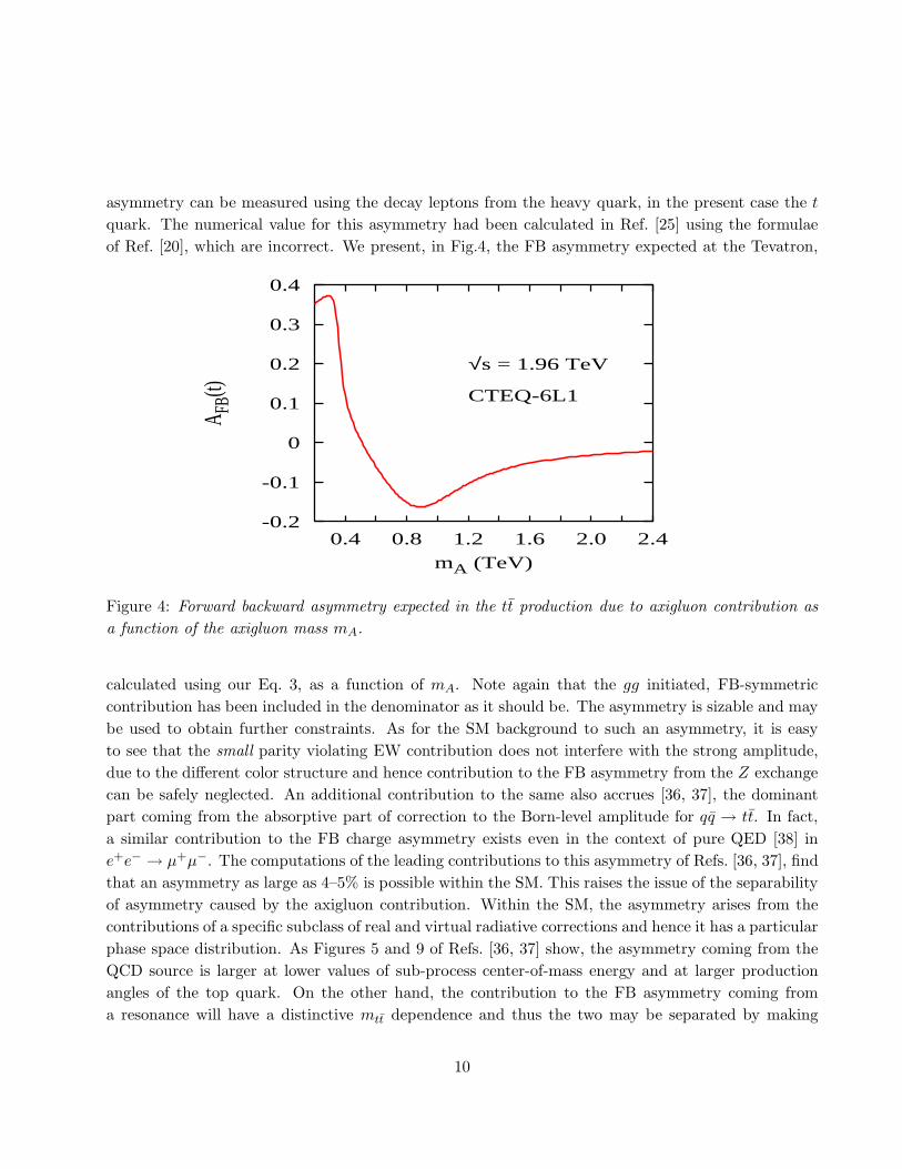
asymmetry can be measured using the decay leptons from the heavy quark, in the present case the t

quark. The numerical value for this asymmetry had been calculated in Ref. [25] using the formulae

of Ref. [20], which are incorrect. We present, in Fig.4, the FB asymmetry expected at the Tevatron,

-0.2

-0.1

0

0.1

0.2

0.3

0.4

0.4 0.8 1.2 1.6 2.0 2.4

A FB(t)

mA (TeV)

√s = 1.96 TeV

CTEQ-6L1

Figure 4: Forward backward asymmetry expected in the tt production due to axigluon contribution as

a function of the axigluon mass mA.

calculated using our Eq. 3, as a function of mA. Note again that the gg initiated, FB-symmetric

contribution has been included in the denominator as it should be. The asymmetry is sizable and may

be used to obtain further constraints. As for the SM background to such an asymmetry, it is easy

to see that the small parity violating EW contribution does not interfere with the strong amplitude,

due to the different color structure and hence contribution to the FB asymmetry from the Z exchange

can be safely neglected. An additional contribution to the same also accrues [36, 37], the dominant

part coming from the absorptive part of correction to the Born-level amplitude for qq → tt. In fact,

a similar contribution to the FB charge asymmetry exists even in the context of pure QED [38] in

e+e− → µ+µ−. The computations of the leading contributions to this asymmetry of Refs. [36, 37], find

that an asymmetry as large as 4–5% is possible within the SM. This raises the issue of the separability

of asymmetry caused by the axigluon contribution. Within the SM, the asymmetry arises from the

contributions of a specific subclass of real and virtual radiative corrections and hence it has a particular

phase space distribution. As Figures 5 and 9 of Refs. [36, 37] show, the asymmetry coming from the

QCD source is larger at lower values of sub-process center-of-mass energy and at larger production

angles of the top quark. On the other hand, the contribution to the FB asymmetry coming from

a resonance will have a distinctive mtt dependence and thus the two may be separated by making

10

appropriate cuts on these two quantities. Such a study, though interesting, is beyond the scope of the

present investigation. In view of the use of FB asymemtry in searching for unusual tt resonances, an

analysis of this asymmetry taking into account higher order effects is certainly worth doing, but again

quite beyond the scope of the current work.

5 tt production at the LHC due to coloron/axigluons

The situation of course is very different at the LHC as the qq fluxes are substantially smaller than

the gg fluxes and tt production is dominated by contribution from gg initial state. However, this

dominance is less severe as we go to larger tt invariant masses. Since, at the LHC, we would typically

be interested in exploring larger axigluon (coloron) masses, it is wiser to concentrate on a data sample

that has enhanced sensitivity to the mass range in question. Hence, in this case, instead of looking

at the total integrated tt cross-sections, we consider the effect of the axigluon/coloron contribution on

the mtt spectrum. The large size of the top sample expected at the LHC (∼ 8 million pairs for 10 fb−1

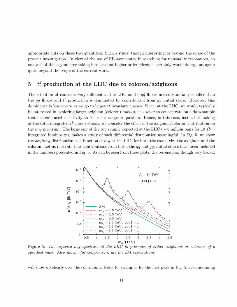
integrated luminosity), makes a study of such differential distribution meaningful. In Fig. 5, we show

the dσ/dmtt distribution as a function of mtt at the LHC for both the cases, viz. the axigluon and the

coloron. Let us reiterate that contributions from both, the qq and gg, initial states have been included

in the numbers presented in Fig. 5. As can be seen from these plots, the resonances, though very broad,

1

10

10 2

10 3

10 4

10 5

10 6

0.5 1 1.5 2 2.5 3 3.5 4 4.5

d σ

/ d m

tt [fb

/ Te

V]

mtt [TeV]

√s = 14 TeV

CTEQ-6L1

SMmA = 1.5 TeVmA = 2.5 TeVmA = 3.5 TeVmC = 1.5 TeV, cot ξ = 1mC = 2.5 TeV, cot ξ = 1mC = 3.5 TeV, cot ξ = 1

Figure 5: The expected mtt spectrum at the LHC in presence of either axigluons or colorons of a

specified mass. Also shown, for comparison, are the SM expectations.

will show up clearly over the continuum. Note, for example, for the first peak in Fig. 5, even assuming

11

a 10% efficiency, there will be about ∼ 104 events at 10 fb−1. This should allow a cross-section

measurement to a % level. It may also be noticed that, precisely at the resonance, the cross-sections

for the axigluon and the coloron for cot ξ = 1 for the same mass are indeed the same. (For, at that

point, the additional cross section is well-approximated by σ(pp → A/C) × Br(A/C → tt), and for

such large values of the boson masses, the branching fractions are nearly identical.) The distributions

also show evidence of the aforementioned interference effects in case of the coloron. While this is

destructive for mtt < mC , it is the opposite for mtt > mC . It can be easily seen that, for the same

mass, the coloron cross-section should be asymptotically bigger than the axigluon cross-section by

about a factor 2 as is seen in Fig. 5.

The LHC being a pp machine, the possibility of constructing a FB asymmetry does not exist.

Since the axigluon has only a pure pseudo-vectorial coupling, a measurement of the net t polarisation

will also not probe the difference in the nature of the coupling between the axigluon and the coloron

unlike the case of (say) an extra Z ′ present in many extensions of the Standard Model [15]. Indeed

as Eqs.(1&4) show, the only dependence on polarizations is through the product of the two (t and

t) helicities and thus only a variable sensitive to this product can exploit this aspect. An example is

afforded by

R∆(mtt) ≡[∫ mtt+∆

mtt−∆

dmttdσ−

dmtt

] [∫ mtt+∆

mtt−∆

dmttdσ+

dmtt

]−1

, (8)

where σ± refer to the cross sections for the product of the t and t helicities to be ±1 respectively.

Ideally, the interval ∆ is to be chosen so as to maximize the sensitivity, and would nominally be a

function of the width of the boson in question and the experimental accuracy in measuring mtt. Rather

than do this, we adopt two nominal values of ∆ = 0.1mBoson and ∆ = 0.2mBoson, given the fact that

the first choice well approximates ∆ ≃ ΓBoson.

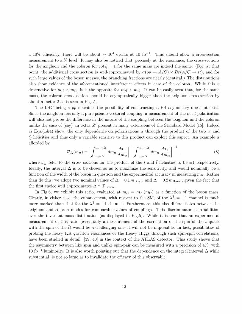
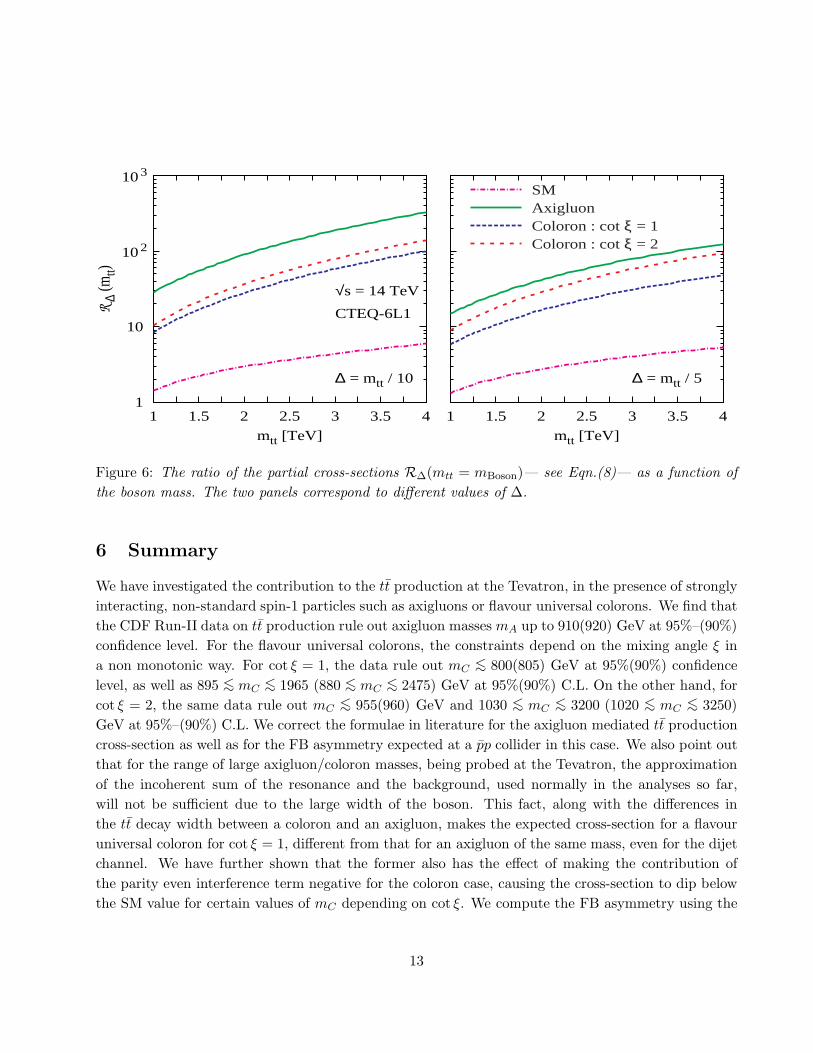
In Fig.6, we exhibit this ratio, evaluated at mtt = mA (mC) as a function of the boson mass.

Clearly, in either case, the enhancement, with respect to the SM, of the λλ = −1 channel is much

more marked than that for the λλ = +1 channel. Furthermore, this also differentiates between the

axigluon and coloron modes for comparable values of couplings. This discriminator is in addition

over the invariant mass distribution (as displayed in Fig.5). While it is true that an experimental

measurement of this ratio (essentially a measurement of the correlation of the spin of the t quark

with the spin of the t) would be a challenging one, it will not be impossible. In fact, possibilities of

probing the heavy KK graviton resonances or the Heavy Higgs through such spin-spin correlations,

have been studied in detail [39, 40] in the context of the ATLAS detector. This study shows that

the asymmetry between like spin and unlike spin-pair can be measured with a precision of 4%, with

10 fb−1 luminosity. It is also worth pointing out that the dependence on the integral interval ∆ while

substantial, is not so large as to invalidate the efficacy of this observable.

12

1

10

10 2

10 3

1 1.5 2 2.5 3 3.5 4

R ∆

(mtt)

mtt [TeV]

√s = 14 TeV

CTEQ-6L1

∆ = mtt / 10

1 1.5 2 2.5 3 3.5 4

mtt [TeV]

∆ = mtt / 5

SMAxigluonColoron : cot ξ = 1Coloron : cot ξ = 2

Figure 6: The ratio of the partial cross-sections R∆(mtt = mBoson)— see Eqn.(8)— as a function of

the boson mass. The two panels correspond to different values of ∆.

6 Summary

We have investigated the contribution to the tt production at the Tevatron, in the presence of strongly

interacting, non-standard spin-1 particles such as axigluons or flavour universal colorons. We find that

the CDF Run-II data on tt production rule out axigluon masses mA up to 910(920) GeV at 95%–(90%)

confidence level. For the flavour universal colorons, the constraints depend on the mixing angle ξ in

a non monotonic way. For cot ξ = 1, the data rule out mC <∼ 800(805) GeV at 95%(90%) confidence

level, as well as 895 <∼ mC<∼ 1965 (880 <∼ mC

<∼ 2475) GeV at 95%(90%) C.L. On the other hand, for

cot ξ = 2, the same data rule out mC<∼ 955(960) GeV and 1030 <∼ mC

<∼ 3200 (1020 <∼ mC<∼ 3250)

GeV at 95%–(90%) C.L. We correct the formulae in literature for the axigluon mediated tt production

cross-section as well as for the FB asymmetry expected at a pp collider in this case. We also point out

that for the range of large axigluon/coloron masses, being probed at the Tevatron, the approximation

of the incoherent sum of the resonance and the background, used normally in the analyses so far,

will not be sufficient due to the large width of the boson. This fact, along with the differences in

the tt decay width between a coloron and an axigluon, makes the expected cross-section for a flavour

universal coloron for cot ξ = 1, different from that for an axigluon of the same mass, even for the dijet

channel. We have further shown that the former also has the effect of making the contribution of

the parity even interference term negative for the coloron case, causing the cross-section to dip below

the SM value for certain values of mC depending on cot ξ. We compute the FB asymmetry using the

13

corrected formulae and show that it can be used to discriminate the axigluon contribution from the

SM as well as from the coloron case. We further find that at the LHC, in spite of the dominance of the

gg initial state, the axigluon/coloron contribution can be seen clearly in the mtt spectrum. We further

suggest a variable constructed using top/anti-top polarizations which can discriminate the axigluon

or coloron contribution from that of a gluon as well as from each other.

Acknowledgments

We wish to acknowledge discussions with Prof. S.D. Rindani. D.C. acknowledges support from the

Department of Science and Technology, India under project number SR/S2/RFHEP-05/2006. R.M.G.,

R.K.S and K.W. wish to acknowledge support from Indo French Centre for Promotion of Advanced

Research Project 3004-B.

References

[1] LEP Electroweak Working Group,

http://lepewwg.web.cern.ch/LEPEWWG/

[2] J. Alcaraz et al. [LEP Collaboration], arXiv:hep-ex/0612034.

[3] For a review, see for example, R. M. Godbole, hep-ph/0205114, Part A, Volume 4, Jubilee Issue

of the Indian Journal of Physics, pp. 44-83, 2004, Guest Editors: A. Raychaudhury and P. Mitra.

[4] C. T. Hill and E. H. Simmons, Phys. Rept. 381 (2003) 235–402, hep-ph/0203079.

[5] See for example discussions in, G. Weiglein et al. [LHC/LC Study Group], Phys. Rept. 426 (2006)

47 [arXiv:hep-ph/0410364].

[6] C. T. Hill and S. J. Parke, Phys. Rev. D 49, 4454 (1994) [arXiv:hep-ph/9312324].

[7] S. Cabrera [CDF and D0 Collaboration], FERMILAB-CONF-06-228-E, Jul 2006. 4pp. Presented

at 14th International Workshop on Deep Inelastic Scattering (DIS 2006), Tsukuba, Japan, 20-24

Apr 2006.

[8] K. Lannon [CDF Collaboration], arXiv:hep-ex/0612009.

[9] M. Beneke et al., arXiv:hep-ph/0003033 and references therein.

[10] M. Guchait, F. Mahmoudi and K. Sridhar, arXiv:hep-ph/0703060.

[11] K. Agashe, A. Belyaev, T. Krupovnickas, G. Perez and J. Virzi, arXiv:hep-ph/0612015.

14

[12] B. Lillie, L. Randall and L. T. Wang, arXiv:hep-ph/0701166.

[13] M. Arai, N. Okada, K. Smolek and V. Simak, Phys. Rev. D 70, 115015 (2004)

[arXiv:hep-ph/0409273]; Phys. Rev. D 75 (2007) 095008 [arXiv:hep-ph/0701155].

[14] R. M. Harris, C. T. Hill and S. J. Parke, arXiv:hep-ph/9911288.

[15] G. Azuelos, B. Brelier, D. Choudhury, P.-A. Delsart, R.M. Godbole, S.D. Rindani, R.K. Singh

and K. Wagh, in arXiv:hep-ph/0602198; 197-205.

[16] P. H. Frampton and S. L. Glashow, Phys. Lett. B 190, 157 (1987).

[17] P. H. Frampton and S. L. Glashow, Phys. Rev. Lett. 58, 2168 (1987).

[18] R. S. Chivukula, A. G. Cohen and E. H. Simmons, Phys. Lett. B 380, 92 (1996)

[arXiv:hep-ph/9603311].

[19] J. Bagger, C. Schmidt and S. King, Phys. Rev. D 37, 1188 (1988).

[20] L. M. Sehgal and M. Wanninger, Phys. Lett. B 200 (1988) 211.

[21] F. Abe et al. [CDF Collaboration], Phys. Rev. D 55, 5263 (1997) [arXiv:hep-ex/9702004].

[22] M. P. Giordani [CDF and D0 Collaborations], Eur. Phys. J. C 33, S785 (2004).

[23] M. A. Doncheski and R. W. Robinett, Phys. Rev. D 58, 097702 (1998) [arXiv:hep-ph/9804226].

[24] For more details, see, W. M. Yao et al. [Particle Data Group], J. Phys. G 33 (2006) 1.

[25] M. A. Doncheski and R. W. Robinett, [arXiv:hep-ph/9706490].

[26] C. T. Hill, Phys. Lett. B 266, 419 (1991).

[27] C. T. Hill, Phys. Lett. B 345 (1995) 483 [arXiv:hep-ph/9411426].

[28] D. A. Dicus, B. Dutta and S. Nandi, Phys. Rev. D 51, 6085 (1995) [arXiv:hep-ph/9412370].

[29] E. H. Simmons, Phys. Rev. D 55, 1678 (1997) [arXiv:hep-ph/9608269].

[30] M. B. Popovic and E. H. Simmons, Phys. Rev. D 58, 095007 (1998) [arXiv:hep-ph/9806287].

[31] R. S. Chivukula, B. A. Dobrescu and J. Terning, Phys. Lett. B 353, 289 (1995)

[arXiv:hep-ph/9503203].

[32] I. Bertram and E. H. Simmons, Phys. Lett. B 443 (1998) 347 [arXiv:hep-ph/9809472].

[33] B. L. Combridge, Nucl. Phys. B 151 (1979) 429.

15

[34] J. Pumplin, D. R. Stump, J. Huston, H. L. Lai, P. Nadolsky and W. K. Tung, JHEP 0207 (2002)

012 [arXiv:hep-ph/0201195].

[35] J. M. Campbell, J. W. Huston and W. J. Stirling, Rept. Prog. Phys. 70 (2007) 89

[arXiv:hep-ph/0611148].

[36] J. H. Kuhn and G. Rodrigo, Phys. Rev. Lett. 81, 49 (1998) [arXiv:hep-ph/9802268].

[37] J. H. Kuhn and G. Rodrigo, Phys. Rev. D 59, 054017 (1999) [arXiv:hep-ph/9807420].

[38] F. A. Berends, K. J. F. Gaemers and R. Gastmans, Nucl. Phys. B 63, 381 (1973).

[39] K. Smolek and V. Simak, Czech. J. Phys. 54 (2004) A451.

[40] F. Hubaut, E. Monnier, P. Pralavorio, K. Smolek and V. Simak, Eur. Phys. J. C 44S2 (2005) 13

[arXiv:hep-ex/0508061].

16