arX

iv:h

ep-p

h/03

1004

2v1

3 O

ct 2

003

MCTP-03-42hep-ph/0310042September 2003

Bs → µµ as a Probe of tanβ at the Tevatron

G.L. Kane 1, Christopher Kolda 2 and Jason E. Lennon 2

1 Michigan Center for Theoretical Physics, University of Michigan, Ann Arbor,

MI 48109, USA2 Department of Physics, University of Notre Dame, Notre Dame, IN 46556, USA

Abstract

Recently it has been understood that flavor-changing processes mediated byHiggs bosons could be a new and powerful tool for discovering supersymmetry.In this paper we show that they may also provide an important method forconstraining the parameters of the minimal supersymmetric standard model(MSSM). Specifically, we show that observation of Bs → µ+µ− at the Tevatronimplies a significant, model-independent lower bound on tan β in the MSSM.This is very important because tan β enters crucially in predictions and in-terpretations of the MSSM, though it is difficult to measure. Within specificmodels, or with other data, the bound becomes significantly stronger.

Over the next several years, the Tevatron at Fermilab will be searching for signs ofphysics beyond the Standard Model (SM), by directly producing and observing newparticles, and by observing rare processes at rates inconsistent with SM predictions. Inthe latter category falls the search for the rare flavor-changing neutral current (FCNC)decay B0

s → µ+µ−. Observation of this decay at the Tevatron would necessarily implynew physics since the predicted rate for this process in the SM is far below the searchcapabilities of the machine. However, supersymmetry (SUSY) naturally predicts largeenhancements in the decay rate mediated by neutral Higgs bosons [1, 2, 3, 4], andin some cases yields branching ratios three orders of magnitude above the SM. Soobservation of the decay would be strong, albeit indirect, evidence in favor of SUSY.

But observation of Bs → µµ actually tells us more. We will show that it is possibleto deduce bounds on the fundamental SUSY parameter tan β, the ratio of the twoHiggs expectation values, from a signal. This is particularly important because tanβis very difficult to measure — there is no general technique for measuring it at hadroncolliders — yet almost all SUSY observables depend on it. And a lower limit may bealmost as useful as an actual measurement because many SUSY observables quicklysaturate as tanβ increases. But we can obtain a limit precisely because the ratefor Bs → µµ does not saturate. Instead it is strongly dependent on tanβ, rising(and falling) as tan6 β. As a secondary feature, we will also be able to obtain someinformation on the mass scale of the new SUSY Higgs bosons, since the branchingratio scales as the fourth power of their masses.

We will begin by considering two very general scenarios in which all flavor mixingdoes/does not come from the CKM matrix and in each case we will arrive at a verystrong bound. But we will also consider some specific models of SUSY breaking andshow that even more stringent bounds can be obtained for these. Our focus willremain on the Tevatron because it has especially good sensitivity to the signal evenif it does not reach its full luminosity potential. However the B-factories and LHCcan also use this, and related processes, to further probe tanβ and the Higgs sector.Unfortunately, if a signal is not seen, non-observation cannot be used to draw absoluteconclusions about the parameter space of the MSSM other than to rule out specificmodel points. It is always possible to choose SUSY parameters in such a way to pushthe signal down to the level of the Standard Model where it would not be observed.

1 Higgs-Mediated B → µµ

First, a little theoretical background. The question of flavor-changing neutral cur-rents (FCNCs) mediated by Higgs bosons was first addressed two decades ago byGlashow and Weinberg [5]. It had always been obvious that the Higgs boson ofthe minimal standard model could not have flavor-violating couplings since the cou-plings of fermions to the Higgs field defines the fermion mass eigenstates and thusalso defines our notion of flavor. But in models with two (or more) Higgs fields,the fermion mass eigenbasis can be different from the Higgs interaction eigenbasis

1

xxx

δLL

23 δRR

23

(b)(a)

bR

t~R

Hu~

H~

d

Hu*

t~Lb

R

~

bR

Hu*

g~

sL

~

bL

~

~g

bL

Hu*

g~~g

Ls s L s R

bL

~

sR

~

bR

~

Figure 1: New contributions to the d-type quark masses in a minimal flavor model [(a)] andin general [(a) and (b)].

and thus Higgs-mediated FCNCs can occur. In order to avoid large FCNCs incon-sistent with experiment, the authors of Ref. [5] proposed several solutions. One ofthose solutions is the “type II” two-Higgs-doublet model: one Higgs field (Hu) cou-ples only to up-type quarks, while the other (Hd) couples only to the down-type:L = QLYUURHu + QLYDDRHd. This guarantees the alignment of the Higgs bosoninteraction eigenbasis with the fermion mass eigenbasis. Such a structure can be pro-tected from quantum corrections by any number of discrete symmetries under whichthe two Higgs fields transform differently.

The MSSM possesses the structure of a type-II model classically. But it possessesno discrete symmetry which can protect this structure; all such symmetries are brokenby the µ-term in the superpotential, which must be present to avoid disagreementwith experiment. And though the type-II structure is also protected by holomorphyof the superpotential, this too is ineffective after SUSY is broken. Thus new termsare generated in the low-energy Lagrangian of the MSSM of the form QLYUURH†

d +QLYDDRH†

d. Whether such terms will lead immediately to FCNCs depends on thestructure of the new YU,D Yukawa matrices [1, 2, 3, 4].

In Ref. [1] it was shown that there are contributions to YD which are flavor-violating and can have important effects at large tanβ. It is actually quite easy to seewhy. Consider the diagram in Fig. 1(a) in which charged higgsinos propagate insidethe loop. If we work in a basis in which the down quarks couple diagonally to H±

d ,then the up quarks have off-diagonal couplings to H±

u proportional to CKM elements.In particular, the coupling of H±

d to bLbR is just the bottom Yukawa coupling, yb. Butthe coupling of H±

u to sLtR is then ytVts where yt is the top-quark Yukawa coupling.Thus the diagram generates a new interaction sLbRH†

u with coefficient proportional toybytVts. We can rewrite this coefficient as simply ybǫ, where ǫ includes not only ytVts

but also the loop kinematic and suppression factors. (We ignore the phases inducedby the sparticles in the loops; work including them is under way [6].)

When Hu gets a vev (vu), it contributes an off-diagonal piece to the fermion massmatrix:

L =(

sR bR

) ( ms 0ybǫvu mb

) (sL

bL

). (1)

This Lagrangian is written in the Higgs interaction eigenbasis of the fermions, which

2

at tree-level is also the mass eigenbasis; we drop the first generation for simplicity.The mass matrix can be diagonalized by a biunitary transformation which mixes thesL and bL by an angle sin θ ≃ ybǫvu/mb. But since mb = yb〈Hd〉 = ybvd, we havesin θ ≃ ǫ tanβ. So although ǫ is one-loop suppressed, the factor of tanβ can allowsin θ to be O(1).

At tree-level, a bb →Higgs transition is possible, with the Higgs decaying toleptons, as in Fig. 2. This occurs by exchange of Hd. However the coupling of thed-quark sector to Hu has shifted the d-quark interaction eigenstates away from theirmass eigenstates. In order to replace the interaction eigenstates on the external legswith mass eigenstates, we must replace

bL → b′L = cos θ bL + sin θ sL (2)

which induces a bRsL → µµ transition through an Hd Higgs, Fig. 2. Then the flavor-changing amplitude bs → µµ is related to the flavor conserving amplitude bb → µµby

Abs→µµ ≃ sin θAbb→µµ. (3)

There are several noteworthy properties of the Higgs-mediated FCNCs. First, theamplitude for Bs → µµ scales as tan3 β at large tanβ. One factor of tan β come fromsin θ, the other two come from the b- and µ-Yukawa couplings which scale as 1/ cosβ.Thus the branching ratio scales as tan6 β and provides an incredibly powerful toolfor constraining tanβ. Second, at large tan β, the Hd Higgs doublet is essentiallydecoupled from the electroweak symmetry breaking. It contains the physical statesH0, A0 and H± which all have roughly equal masses. But because Higgs flavorchanging must disappear in a model with only one Higgs doublet, the FCNC branchingratios must decouple as m4

A. But this does not mean that the effects decouple as theSUSY mass scale increases. Rather, in the limit that all supersymmetric masses aretaken heavy, while A0 (or Hd) remains light, the rate for Higgs FCNCs approachs afinite constant.

What diagrams contribute to the off-diagonal Higgs couplings? First, even if allflavor violation stems from the CKM matrix alone, there is the one-loop higgsinodiagram of Fig. 1(a) already considered. Models with only this CKM-induced flavorviolation are known as “minimal flavor violation” (MFV) models. Note that thiskind of flavor violation has nothing to do with the “SUSY flavor problem.” It isalways present in SUSY because it is generated by the flavor violation in the CKMmatrix and cannot be eliminated simply by making superpartners heavy or by aligningquark/squark mass matrices.

More generally there are also gluino loop diagrams contributing to the same in-teractions (Figure 1(b)), if flavor-violating LL or RR squark mass insertions arenon-zero. Such an insertion can be generated in minimal models by renormalizationgroup running of the squark mass matrices, or may appear in the underlying theory.We make no assumptions in our general analysis about the underlying source of thisflavor-changing in the squark sector, and we refer to this as general flavor violation.

3

b_

b_

������������

µ

µs H

b_

������������

µ

µb H������������

µ

µHb’

cosθ sinθd

L

R

dL

R

dL

R

= +

Figure 2: Diagram for bb →Higgs→ µµ in the interaction (primed) eigenbasis becomesbs →Higgs→ µµ in the mass eigenbasis, suppressed by sin θ, the sL–bL mixing angle.

Because this new source of FCNCs emerges from the Higgs sector, it preferentiallygenerates processes involving heavy fermions. Thus the channels in which Higgs-mediated FCNCs can most easily be observed are Bs,d → ττ and Bs,d → µµ. Thechannels with final state muons are suppressed relative to those with final state tausby (mµ/mτ )

2 but are much cleaner experimentally. The channels with initial stateBd are suppressed relative to Bs by (Vtd/Vts)

2. Thus a machine which produces anabundance of Bs and can cleanly tag and measure muons is ideal for studying thisphysics. This machine is precisely the Tevatron, either in CDF or D0. The currentlimits on Br (Bs,d → µµ) are provided by CDF from Run I at 2.0×10−6 and 6.8×10−7

respectively. Given enough luminosity, the B-factories may be able to corroborateany Tevatron discovery using Bd → µµ or, if a suitable technique is found, Bd → ττ .

If CDF and D0 each record even 2 fb−1 of data during Run II of the Tevatron,now underway, they can probe the Bs → µµ branching fraction below the 10−7 level.(See, e.g., Ref. [8] for a more detailed study of the CDF capabilities.) We will forillustration assume that the Tevatron can discover a signal in B → µµ if its branchingratio is greater than 10−7. Because the branching ratios scale as high powers of theinput parameters (m4

A and tan6 β), small changes in the Tevatron capabilities willgenerate infinitessimal changes in our results. And once a signal is discovered, thenumerical analysis can be redone to obtain more precise limits.

We demonstrate below that there is a minimum value of tanβ consistent with asignal at the 10−7 level, and calculate it. We also consider the interplay between thepseudoscalar mass and tan β, a result which could be important in searches for theadditional Higgs bosons at future colliders. Both of these analyses will be done in fullgenerality within the MSSM. We will not constrain ourselves initially to any particularclass of MSSM models, such as supergravity- or anomaly-mediated SUSY-breaking.This can be done because there are only a limited number of parameters on which thebranching ratio will depend and these few parameters can be studied without furthersimplifications or assumptions. However in particular classes of models the constraintson tan β and mA are stronger and therefore observation of a signal provides even moreinformation. We will consider specific SUSY models after doing the general analysisand we will find bounds on tan β much stronger than in the general case.

4

2 Minimal Flavor Violation: Higgsino Contribution

Regardless of any details of SUSY-breaking, the higgsino contribution of Fig. 1(a) toHiggs-mediated flavor-changing processes must be present. First we will consider thecase where only this contribution is present and then generalize in the next section.Thus we begin by considering the MFV models.

The flavor-changing contribution of the higgsino loop diagram is encoded in a newdimensionless parameter κ

Hsuch that

Br (Bs → µµ) ≃ G2F

8πη2

QCDm3Bs

f 2Bs

τBsm2

b m2µ

(tan2 β

cos4 β

)(κ2

H

m4A

). (4)

Here ηQCD ≃ 1.5 is the QCD correction due to running between the SUSY and Bs

scales, and we take fBs= 220 MeV. Note that the fraction tan2 β/ cos4 β approaches

tan6 β at large tanβ.The parameter κ

His calculated to be [1]

κH

= −GF m2t VtsVtb

4√

2π2 sin2 βµAt f(µ2, m2

tL, m2

tR) (5)

where mtLand mtR

are the left- and right-handed top squark masses, µ is the super-potential Higgs mass parameter, At is the top-squark trilinear term, and the functionf is defined in Ref. [1]. The important thing to know about f is that it is positivedefinite, symmetric in its inputs and f(x, y, z) ∼ 1/max(x, y, z) up to a constant ofO(1). In particular, f(m2, m2, m2) = 1/(2m2) and f(m2, m2, 0) = 1/m2.

In order to maximize the function κH

(and therefore maximize the branchingfraction one can obtain for a given {mA, tan β}) we need only consider the four pa-rameters m2

tL, m2

tR, µ and At. This is easiest to do by considering the limits in which

κH

could become large.First consider the limit in which µ is much larger than the squark masses. Then

κH∼ At/µ since µ appears both in f and as a prefactor. Thus it appears that κ

Hcan

grow unabated as At becomes large. Such a runaway behavior would generate arbi-trarily large branching ratios and invalidate our claim to a bound on tan β. However,there is a “cosmological” limit to At: as At increases far beyond the squark masses,the usual electroweak vacuum become unstable with the true vacuum breaking QEDand QCD [9]. We apply this constraint by applying the famous condition

A2t < 3 (m2

tL+ m2

tR+ m2

2). (6)

(The last term, m22, is the mass parameter for Hu appearing in the Higgs potential.

Since m22 < 0 is necessary to break the electroweak symmetry, we can maximize At

by setting m22 = 0.) Because the squark masses are much smaller than µ in this limit,

then At/µ can not become much larger than unity at best. A similar argument holds

5

100 200 300 400 500 600 700 800 900 1000

mA

[GeV]

10

20

30

40

50

60

tan

β

1x10-63x10-7

1x10-7

3x10-8

1x10-8

MFV

Figure 3: Contours of maximum allowed value for Br (Bs → µµ) (labelled) as a function of{mA, tan β} for minimal flavor violation. For a given branching ratio, the allowed region isabove the labelled line.

for large At but with µ smaller than the squark masses, except now κH

is more highlysuppressed, κ

H∼ Atµ/m2

t.

The actual limit is obtained when µ becomes large along with one of the squarkmasses (with the other as small as possible). Then f(· · ·) → 1/µ2. But the QED/QCD-breaking constraint still limits At, though now it becomes At <

√3µ so that µAtf <√

3 which implies that

κH

<0.011

sin2 β. (7)

Plugging into Eq. (4) immediately gives

Br (Bs → µµ) <5 × 10−6 GeV4

m4A cos6 β

. (8)

Thus for mA = 100 GeV (approximately its current lower limit) and a branching ratiogreater than 10−7, we deduce in an MFV scenario that tanβ > 11. As mA increases,the bound on tan β also increases rapidly; for example, if mA > 200 GeV, one musthave tanβ > 18. In general,

tanβ > 11(

mA

100 GeV

) 2

3

[Br (Bs → µµ)

1 × 10−7

] 1

6

(9)

where we have taken 1/ cosβ ≃ tanβ for large tanβ.In Figure 3, we plot contours representing the maximal value of the Bs → µµ

branching ratio consistent with a given choice of mA and tan β. Given a measuredvalue of the branching ratio, only the region above the line is consistent in an MFVscenario.

6

3 General Flavor Violation: Gluino Contributions

In the case of MFV, only the higgsino loop has any significant effect in producingflavor violation. However once one moves away from truly minimal flavor violation,a new source arises. In a truly general scenario, the g-q-q couplings can be flavorchanging. In the mass insertion approximation, these violations are moved to thesquark propagators where they appear as bilinear interactions which mix flavors andeven chiralities of the squarks. The size of the insertions is parametrized by a dimen-sionless quantity, δij

ab = (∆m2ab)ij/m

2ab where a, b are either L or R, and i, j label the

squark generation. We are only interested in the down-sector δ23LL and δ23

RR insertionsfor this work. At present there are no strong experimental bounds on these inser-tions and so it is possible that the sL and bL (or sR and bR) are maximimally mixed,or δ23

LL,RR ≃ 1. Of course, in particular models a large δ23LL,RR could lead to large

B → K∗γ or B → φKS, but constraints from these processes are sensitive to δ23ab/m

2ab

while B → µµ is sensitive to δ23ab alone. Since we allow very large flavor-mixing,

we must take care to note that the mass insertion approximation breaks down as δapproaches one; we will discuss this issue shortly.

The new gluino-induced source of flavor changing in general models generates newdiagrams in Bs → µµ with b and s squarks and gluinos in the loop; see Fig. 1(b).For our purposes here we can ignore the higgsino contributions since their maximalsize is smaller than that of the gluino loop if δ23

LL,RR ∼ 1. We will also assume thatonly one of the two diagrams in Fig. 1(b) dominates the branching ratio; when thereis data, a fully combined analysis should be done. Specifically we will choose the δ23

LL

diagram to dominate, though our results are identical if the δ23RR diagram dominates

instead. We will discuss more realistic scenarios at the end of the section.We parametrize the gluino contribution as

κg =2αs

3πδ23LL µM3f2(m

2sL

, m2

bL

, m2

bR

, M23 ) (10)

where the function f2 is defined in Ref. [7]. The branching ratio is calculated from κg

just as for κH

in Eq. (4). Notice in particular the lack of a Vts suppression in κg; thiswill allow much smaller values of tan β to be consistent with an experimental signal.

There are two limits in which we can simplify the above expression. For smallbL–sL mixing, we can usually take m2

sL

= m2

bL

in Eq. (10) and then work in the mass

insertion approximation. However, if there is a large hierarchy in between sL andbL, or if there is large mixing, that approximation breaks down. Instead, it is fareasier to work directly in the basis of the mass eigenstates. Defining dLi (i = 1, 2)as bL cos θ + sL sin θ and its orthogonal combination, we must replace the productδ23LLf2(· · ·) in Eq. (10) with

cos θ sin θ{f(m2

dL1

, · · ·) − f(m2

dL2

, · · ·)}

<1

2f(m2

dL1

, · · ·). (11)

7

The inequality follows only from the positivity of the function f . Given more infor-mation in the future about the squarks (masses or lower bounds) it may be possibleto find a lower bound on the second term and thus an improved upper bound on thebranching fraction.

Like the MFV case there is a possible runaway behavior in computing the dia-grams in Fig. 1(b), allowing for arbitrarily large branching ratios. In the MFV case,this arose as At → ∞, which we cut off by demanding that color-breaking minimadeeper than the SM minimum not appear. In a general case, this arises as µ → ∞for which the color-breaking constraint is useless. However there are equally powerfulconstraints which rely on fine-tuning arguments, which have recently been strength-ened [12]. In particular, the µ-parameter appears in the Higgs potential and it isthe minimization of this potential which must supply the weak scale. There is awell-known relation among the µ-term and other Higgs soft mass terms which musttogether generate the scale mZ :

1

2m2

Z =m2

Hd− m2

Hutan2 β

tan2 β − 1− µ2. (12)

If |µ| ≫ mZ then a fine-tuning must be arranged among mHu, mHd

and µ in orderto generate mZ on the left hand side of the Eq. (12). We will require |µ| < 500 GeV,which is a statement that we allow less fine-tuning in the electroweak potential thanabout one part in 60. However in our expressions we will show how to scale ourresults for other choices of µ, in case the reader wishes to apply their own fine-tuningconstraint.

In order to calculate the upper bound on the branching ratio, it is useful to notethat the product M3f(M2

3 , m2qL

, m2qR

) reaches its upper bound when the squarks areas light as possible and degenerate, and M3 ≃ 2.1mq. Then one can derive thesemi-analytic bound (assuming maximal mixing):

κg < 0.009

∣∣∣∣µ

500 GeV

∣∣∣∣ (13)

leading to

Br (Bs → µµ) <3.0 × 10−3 GeV4

m4A

∣∣∣∣µ

500 GeV

∣∣∣∣2

tan6 β. (14)

and

tan β > 4(

mA

100 GeV

) 2

3

[Br (Bs → µµ)

1 × 10−7

] 1

6

∣∣∣∣∣500 GeV

µ

∣∣∣∣∣

1

3

. (15)

Contours of the maximum allowed branching ratio are plotted in Fig. 4 as a functionof mA and tan β for the case of maximal mixing. For small mixing we can return tothe mass insertion approximation in which case

tan β > 7

(0.1

δ23LL

) 1

3(

mA

100 GeV

) 2

3

[Br (Bs → µµ)

1 × 10−7

] 1

6

∣∣∣∣∣500 GeV

µ

∣∣∣∣∣

1

3

. (16)

8

200 400 600 800 1000

mA

[GeV]

0

10

20

30

40

50

tan

β

1x10-6

3x10-7

1x10-7

3x10-8

1x10-8

Generalδ

LL=0.1

Figure 4: Contours of maximum allowed value for Br (Bs → µµ) (labelled) as a function of{mA, tan β} for non-minimal flavor violation with δ23

LL = 0.1. For a given branching ratio,the allowed region is above the labelled line.

The bounds presented in this section should be considered the absolute limitson tan β given a signal at the Tevatron at the 10−7 level. Nowhere did we injecttheoretical constraints stemming from some particular model of SUSY. On the otherhand, if we had a model, or other information, we could devise much stronger bounds.For example, many observables in SUSY depend on µ, so that once SUSY is found,we will very quickly have constraints on µ, which would allow more precise bounds.And if we have some theoretical or experimental reason to believe in a particularmodel of SUSY-breaking, then we know even more. As we will discuss in Section 4,models produce bounds which are much stronger than the general case.

3.1 “Nearly-Minimal” Flavor Violation

For most purposes, the bounds in the previous section are too general. SUSY modelswhich are truly generic and general have an embarassing wealth of flavor-changingmass insertions like δ23

LL. Most of these insertions must be miniscule in order to avoid

dangerously large FCNCs in well-studied processes, such as K0-K0

mixing. Thusone usually imposes on SUSY some form of organizing principle which prevents mostof these insertions from becoming large, whether that be mass degeneracies or massmatrix alignment.

However even in models which naturally solve the SUSY flavor problem, oneusually still expects some flavor violation to reappear by way of renormalizationeffects. The most common source of these is the presence of the up-quarks Yukawamatrix in the renormalization group equations for the left-handed squarks. Becauseall Yukawa matrices cannot be simultaneously diagonalized, non-zero δij

LL will begenerated. (The RR mass insertions will not be generated at leading order.) However

9

there is a significant difference between these mass insertions and those considered inthe general case above: here δij

LL will be proportional to the corresponding elementof the CKM matrix. For example, δ23

LL will be naturally suppressed by Vts. Thus onetypically finds δ23

LL<∼ O(Vts) which in turn would force tan β >∼ 9 for Br (Bs → µµ) >

10−7. However this bound is not a true limit – the model can be tuned in order toobtain the same branching ratio but with much smaller values of tanβ.

Thus, while one expects from theoretical arguments that tan β must be greaterthan 9 in order to see a signal at the Tevatron, the true mathematical limit remainsat tanβ = 4 as found in the previous section, until the origins of SUSY flavor physicsare better understood.

3.2 Relation to Other Observables

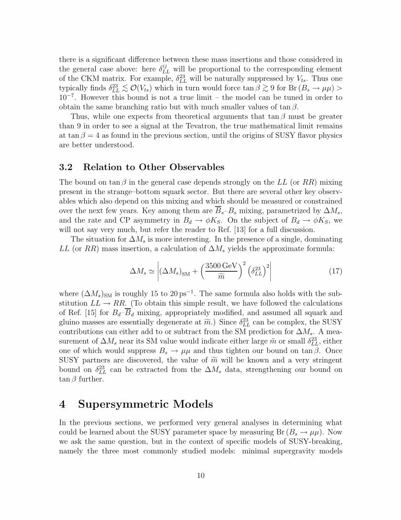
The bound on tan β in the general case depends strongly on the LL (or RR) mixingpresent in the strange–bottom squark sector. But there are several other key observ-ables which also depend on this mixing and which should be measured or constrainedover the next few years. Key among them are Bs–Bs mixing, parametrized by ∆Ms,and the rate and CP asymmetry in Bd → φKS. On the subject of Bd → φKS, wewill not say very much, but refer the reader to Ref. [13] for a full discussion.

The situation for ∆Ms is more interesting. In the presence of a single, dominatingLL (or RR) mass insertion, a calculation of ∆Ms yields the approximate formula:

∆Ms ≃∣∣∣∣∣(∆Ms)SM +

(3500 GeV

m

)2 (δ23LL

)2

∣∣∣∣∣ (17)

where (∆Ms)SM is roughly 15 to 20 ps−1. The same formula also holds with the sub-stitution LL → RR. (To obtain this simple result, we have followed the calculationsof Ref. [15] for Bd–Bd mixing, appropriately modified, and assumed all squark andgluino masses are essentially degenerate at m.) Since δ23

LL can be complex, the SUSYcontributions can either add to or subtract from the SM prediction for ∆Ms. A mea-surement of ∆Ms near its SM value would indicate either large m or small δ23

LL, eitherone of which would suppress Bs → µµ and thus tighten our bound on tanβ. OnceSUSY partners are discovered, the value of m will be known and a very stringentbound on δ23

LL can be extracted from the ∆Ms data, strengthening our bound ontan β further.

4 Supersymmetric Models

In the previous sections, we performed very general analyses in determining whatcould be learned about the SUSY parameter space by measuring Br (Bs → µµ). Nowwe ask the same question, but in the context of specific models of SUSY-breaking,namely the three most commonly studied models: minimal supergravity models

10

(mSUGRA, also called the constrained MSSM), minimal gauge-mediated (GMSB)models, and minimal anomaly-mediated (AMSB) models. Realistic models will nec-essarily yield much stronger bounds on mA and tanβ for two reasons: first, there is noreason for their contributions to FCNCs to be maximal, and second there are oftencorrelations with other processes which suppress the flavor-changing contributions.Several analyses of Bs → µµ in the context of SUSY models have been completed [10]and a more detailed study of this will appear shortly [14]; here we summarize someof the important results of this last study. Namely we will find bounds on tan β inspecific models for an observed Br (Bs → µµ) and discuss their implications.

For each of the three models to be discussed, we will vary all the free parametersof the models and at each “model point” calculate the Bs → µµ branching frac-tion [11]. However we will also apply several phenomenological constraints to avoidpoints which are unphysical. The most important constraints come from the muonmagnetic moment [16] and the b → sγ transition [17]. For the former, we will demandthat the SUSY constributions to (g − 2)µ fall between −5 × 10−10 and 57 × 10−10.For the latter, we will demand that calculated rate for b → sγ fall between 2.1×10−4

and 4.5×10−4. In both cases these are rather wide windows. For the muon magneticmoment, a wide window is required by the inconsistency of the e+e− and τ data setswhich are used to calculate the standard model hadronic contributions to g − 2. Forb → sγ we use a wide window because of the uncertainties in the next-to-leadingorder calculation of the SUSY contributions.

4.1 Minimal supergravity

Minimal supergravity (mSUGRA) actually contributes fairly efficiently to Higgs-mediated FCNCs. It has three key ingredients that help to generate large branchingratios. First, mSUGRA models often have large At trilinear terms, necessary for thehiggsino contribution. Second, the extended running from the GUT scale down to theweak scale generates considerable mixing between the second and third generationsquarks, allowing for a sizable gluino contribution. Finally, the pseudoscalar Higgsdoes not come out particularly heavy.

In Fig. 5(a), we show a scatter plot of points in the mSUGRA model space, eachone representing a distinct choice of tanβ, M1/2, m0, and A0 (we take µ > 0 only),consistent with all experimental and theoretical constraints. There are several impor-tant lessons to draw from the figure. One should immediately note that mSUGRAmodels exist, consistent with all other constraints, that have rates for Bs → µµ rightup to the CDF bound; in fact, models were found that passed all other constraints, ex-cept the Bs → µµ bound, indicating that Bs → µµ is already a non-trivial constrainton mSUGRA models.

We also notice that mSUGRA models with a branching ratio greater than 10−7

require tanβ > 40. Thus observation of Bs → µµ at Run II would certainly indicatevery large tanβ if mSUGRA is the correct model.

11

20 25 30 35 40 45 50 55tanβ

10-9

10-8

10-7

10-6

Br

(Bs→

µµ)

Figure 5: Correlation of tan β and Br (Bs → µµ) in a representative sample of mSUGRAmodels.

One also notices another interesting feature in the figure, namely a bifurcation ofthe points at the largest branching fractions. The points in the upper arm all haveA0 < 0 while all the points with A0 > 0 lie in the main body of points. This behavioris rooted in the b → sγ constraint. For A0 > 0, models with very large Bs → µµalso have chargino contributions to b → sγ which tend to cancel the SM. Thus theresulting Br (b → sγ) is too small and we throw the model point out. As the SUSYmass scales increase, the cancellation goes away, but the rate for Bs → µµ is alsosuppressed. However, the cases with A0 < 0 exhibit a very different behavior. Forlight spectra, these models can have SUSY contributions to b → sγ much larger thanthose of the SM, but with opposite sign, so that after adding the two pieces, theresulting rate is still roughly consistent with the SM and with experiment. Then asthe SUSY mass scale is increased, the two pieces start to cancel to zero, ruling outthe model points. As the SUSY scale is further increased, the SUSY contributiondecouples and the SM once again dominates. Thus a gap is generated where themodels predict Br (b → sγ) ≃ 0.

Thus models with A0 > 0 can only be observed in Run II if tan β > 50 while modelswith A0 < 0 can have tanβ down to 40. The upshot of this is that a measurementof Bs → µµ and an independent measurement of tanβ could indicate that A0 < 0.However, these measurements alone cannot be used to show that A0 > 0.

4.2 Anomaly Mediation

The simplest models with pure anomaly mediation have only one free parameter,an overall mass scale, but are not phenomenologically viable. But one can define a

12

20 25 30 35 40 45 50 55tanβ

10-9

10-8

10-7

10-6

Br

(Bs→

µµ)

Figure 6: Correlation of tan β and Br (Bs → µµ) in a representative sample of AMSBmodels.

“minimal” anomaly-mediated model which has two free parameters: an overall massscale for the anomaly mediation, and a separate mass scale just for the scalars. Weconsidered this minimal model, by varying both of these parameters, as well as tanβ,and studying the resulting spectra. In principle, AMSB shares many of the samefeatures that make mSUGRA a nice candidate for discovery of Bs → µµ. In practice,this is only partially true. In AMSB the b → sγ constraint is much stronger andrules out many model points where a large Higgs-mediated FCNC signal would havebeen predicted. We do not find any models with observable branching fractions ofBs into muons (> 10−7), consistent with the result of Baek et al. [10]. However, wenote that this result depends very strongly on the b → sγ calculation; changes in theNLO calculation could easily allow for much larger (or smaller) Bs → µµ branchingfractions.

A scatter plot of the allowed parameter space is shown in Fig. 6(a). This figureagain shows a bifurcation into two separate regions, though this time much moredistinct than in the mSUGRA case. Here there is no fundamental difference betweenthe two regions, but the basic explanation is similar to the case of the last section.For AMSB models with large tan β and intermediate masses, the SUSY contributionto b → sγ tends to cancel the SM, predicting a rate which is too small. For largemasses, the SUSY contribution decouples, but then so does Bs → µµ. However, thereis a region of very light masses where the SUSY contribution is roughly twice the SMcontribution, but with opposite sign, so that their sum squared is consistent withdata. This last region is the upper-right region of the figure. There we see that onecan have Br (Bs → µµ) are large as 10−7 only if tanβ > 55.

13

30 35 40 45 50 55tanβ

10-9

10-8

10-7

10-6

Br

(Bs→

µµ)

Figure 7: Correlation of tan β and Br (Bs → µµ) in a representative sample of GMSBmodels.

4.3 Gauge Mediation

Unlike the previous two cases, one would not expect a large Higgs-mediated FCNCsignal in models with gauge mediation. Whereas mSUGRA has a large At and lotsof running to generate squark mixing, gauge-mediated models have neither. At themediation scale, At = 0 (so no higgsino contribution) and there is little running unlessthe mediation scale is large (so no gluino contribution). Indeed, we find that it isvery difficult to generate observable signals at the Tevatron for GMSB models, evenwithout invoking constraints from b → sγ. This is best summarized by Fig. 7, whereno models are found with Br (Bs → µµ) above 4 × 10−8, making this signal difficultif not impossible to observe in Run II.

To obtain this figure, we varied all the parameters of the GMSB model, includingthe number of messengers, which we allowed to take values of n5 = 1, 3, and 5. Wealso allowed the messenger scale, M , to go as high as 1014 GeV. At such large M ,one would expect to maximize your signal since both A-terms and squark mixingbenefit from the running between M and mZ . And indeed the maximum signals areoccurring for large messenger scales. However even with such a large scale, there islittle signal in this channel compared to mSUGRA or AMSB models. Thus a signalat the Tevatron tells us something significant that has nothing to do with tanβ — itwould be evidence against gauge mediation itself [10, 14]!

14

5 Conclusions

Over the next several years, the Tevatron’s physics program has a strong opportunityto discover new physics in the rare decay Bs → µµ. And if either CDF or DØ doobserve this signature, they will have simultaneously provided very strong evidence fora supersymmetric world just beyond our current reach. And they will have providedan important insight into SUSY-breaking and its mediation mechanism. And theywill have placed a lower bound on the parameter tanβ, vitally important to futurestudies of SUSY. It is the existence of this lower bound, and its value, that we havederived in this work.

The SUSY parameter tanβ is one of the most important quantities which needsto be measured in a supersymmetric world. In a top-down approach, the calculationof tan β from first principles would be an important test of some underlying theory.In a bottom-up approach, tanβ is a necessary input to the Yukawa sector and thusrelevant to everything from Yukawa unification to radiative electroweak symmetrybreaking. Almost all predictions that can test the form of the underlying theorydepend on tanβ in some way, so it must be measured as a first step in studying andtesting models of SUSY. Yet tan β is infamously difficult to measure, particularly athadron colliders or in rare decays — all methods proposed to date are model and/orparameter dependent.

The decay Bs → µµ may improve the situation dramatically because it is unusu-ally sensitive to tan β, providing an opportunity to bound tanβ if a signal is seen.In this paper we showed that some very general theoretical assumptions that do notdepend on specific models allow us to put significant lower bounds on tanβ given asignal. In the general case with large flavor changing effects allowed (δ23

LL ∼ 1), thebound is given by Eq. (15), leading to tanβ >∼ 4. This bound increases quickly withdecreasing flavor violation: for δ23

LL ≃ 0.1 the bound is pushed to tanβ >∼ 7 (Eq. (16)).In more typical models in which δ23

LL<∼ Vts or Vub, then tan β >∼ 9 if a signal is seen

at the Tevatron. However, the decay Bs → µµ does not require new sources offlavor changing to be present; it can be induced simply from the flavor changing al-ready present in the standard model CKM matrix. In such a case a stronger boundtan β >∼ 11 is obtained (Eq. (9)). These bounds are for a B(Bs → µµ) > 10−7; wehave also shown how to scale the bounds as a function of the branching fraction.Finally, we find that the bounds are significantly stronger in often studied modelssuch as minimal supergravity.

For many purposes, a lower limit is as good as a measurement since many ob-servables (mh, gµ − 2, dark matter signals, etc) saturate as tanβ increases. There isalso an upper limit on tan β of order 60 from the requirement that the theory remainperturbative up to high (unificiation) scales. Thus a lower limit often is tantamountto a measurement.

15

Acknowledgements

We are grateful to K. Hidaka for helpful comments on the manuscript. This workwas supported in part by the National Science Foundation under grant PHY00-98791and by the U.S. Department of Energy under grant DE-FG02-95ER40896.

References

[1] K. S. Babu and C. Kolda, Phys. Rev. Lett. 84, 228 (2000).

[2] C. S. Huang, W. Liao and Q. S. Yan, Phys. Rev. D 59, 011701 (1999);C. Hamzaoui, M. Pospelov and M. Toharia, Phys. Rev. D 59, 095005 (1999);S. R. Choudhury and N. Gaur, Phys. Lett. B 451, 86 (1999);C. S. Huang, W. Liao, Q. S. Yan and S. H. Zhu, Phys. Rev. D 63, 114021 (2001).

[3] C. S. Huang and W. Liao, Phys. Lett. B 525, 107 (2002) and Phys. Lett. B 538,301 (2002);C. Bobeth, T. Ewerth, F. Kruger and J. Urban, Phys. Rev. D 64, 074014 (2001)and Phys. Rev. D 66, 074021 (2002);A. J. Buras, P. H. Chankowski, J. Rosiek and L. Slawianowska, Nucl. Phys. B619, 434 (2001), Phys. Lett. B 546, 96 (2002) and Nucl. Phys. B 659, 3 (2003);G. Isidori and A. Retico, JHEP 0111, 001 (2001) and JHEP 0209, 063 (2002).

[4] A. Dedes, arXiv:hep-ph/0309233.

[5] S. L. Glashow and S. Weinberg, Phys. Rev. D 15, 1958 (1977).

[6] K. Hidaka, G.L. Kane and C. Kolda, in preparation.

[7] K. S. Babu and C. Kolda, Phys. Rev. Lett. 89, 241802 (2002).

[8] R. Arnowitt, B. Dutta, T. Kamon and M. Tanaka, Phys. Lett. B 538, 121 (2002).

[9] J. F. Gunion, H. E. Haber and M. Sher, Nucl. Phys. B 306, 1 (1988).

[10] A. Dedes, H. K. Dreiner and U. Nierste, Phys. Rev. Lett. 87, 251804 (2001);R. Arnowitt, B. Dutta, T. Kamon and M. Tanaka, Phys. Lett. B 538, 121 (2002);S. Baek, P. Ko and W. Y. Song, Phys. Rev. Lett. 89, 271801 (2002) and JHEP0303, 054 (2003);H. Baer et al., JHEP 0207, 050 (2002);A. Dedes, H. K. Dreiner, U. Nierste and P. Richardson, arXiv:hep-ph/0207026;J. K. Mizukoshi, X. Tata and Y. Wang, Phys. Rev. D 66, 115003 (2002);T. Blazek, S. F. King and J. K. Parry, arXiv:hep-ph/0308068.

16

[11] Model points were generated using the package SOFTSUSY:B. C. Allanach, Comput. Phys. Commun. 143, 305 (2002) [arXiv:hep-ph/0104145].

[12] G. L. Kane, J. Lykken, B. D. Nelson and L. T. Wang, Phys. Lett. B 551, 146(2003).

[13] G. L. Kane, P. Ko, H. B. Wang, C. Kolda, J. H. Park and L. T. Wang, arXiv:hep-ph/0212092 and Phys. Rev. Lett. 90, 141803 (2003).

[14] C. Kolda and J. Lennon, in preparation.

[15] D. Becirevic et al., Nucl. Phys. B 634, 105 (2002);P. Ko, J. Park and G. Kramer, Eur. Phys. J. C 25, 615 (2002).

[16] The experimental constraints on (g − 2)µ are based on:G. W. Bennett et al. [Muon g-2 Collaboration], Phys. Rev. Lett. 89, 101804(2002).For theoretical constraints in the context of SUSY see, e.g.:M. Byrne, C. Kolda and J. E. Lennon, Phys. Rev. D 67, 075004 (2003).

[17] The experimental constraints on B(b → sγ) are based on:K. Abe et al. [Belle Collaboration], Phys. Lett. B 511, 151 (2001);S. Chen et al. [CLEO Collaboration], Phys. Rev. Lett. 87, 251807 (2001).For the calculation within SUSY see:M. Ciuchini, G. Degrassi, P. Gambino and G. F. Giudice, Nucl. Phys. B 534, 3(1998);G. Degrassi, P. Gambino and G. F. Giudice, JHEP 0012, 009 (2000);M. Carena, D. Garcia, U. Nierste and C. E. Wagner, Phys. Lett. B 499, 141(2001).

17