arX

iv:h

ep-t

h/93

0800

5v2

3 A

ug 1

993

CERN-TH. 6865/93, HUPAPP-93/3, NEIP 93-004NSF-ITP-93-96, UTTG-13-93

hepth 9308005

2 August 1993

PERIODS FOR CALABI–YAU AND

LANDAU–GINZBURG VACUA

Per Berglund1,2♯, Philip Candelas2,3, Xenia de la Ossa4 ♯, Anamarıa Font5,

Tristan Hubsch6, Dubravka Jancic2, Fernando Quevedo4

1Institute for Theoretical PhysicsUniversity of California

Santa BarbaraCA 93106, USA

2Theory GroupDepartment of PhysicsUniversity of Texas

Austin, TX 78712, USA

3Theory DivisionCERN

CH 1211 Geneva 23Switzerland

4Institut de PhysiqueUniversite de Neuchatel

CH-2000 NeuchatelSwitzerland

5Departamento de FısicaUniversidad Central de Venezuela

A.P. 20513, Caracas 1020-AVenezuela

6Department of PhysicsHoward University

WashingtonDC 20059, USA

ABSTRACT

The complete structure of the moduli space of Calabi–Yau manifolds and theassociated Landau-Ginzburg theories, and hence also of the corresponding low-energy effective theory that results from (2,2) superstring compactification, maybe determined in terms of certain holomorphic functions called periods. Theseperiods are shown to be readily calculable for a great many such models. Weillustrate this by computing the periods explicitly for a number of classes ofCalabi–Yau manifolds. We also point out that it is possible to read off from theperiods certain important information relating to the mirror manifolds.

CERN-TH. 6865/93

2 August 1993

♯ After Sept. 15th: Institute for Advanced Study, Olden Lane, Princeton, NJ 08540, USA.

On leave from the Institute “Rudjer Boskovic”, Zagreb, Croatia.

Contents

1. Preamble

2. Hypersurfaces in Weighted IPN

2.1 Generalities

2.2 The fundamental expansion

2.3 Convergence and analytic continuation: small ϕα

2.4 Convergence and analytic continuation: general ϕα

2.5 The remaining periods

3. CICY Manifolds

3.1 Complete intersections in a single projective space

3.2 Calabi-Yau hypersurfaces in products of projective spaces

3.3 A natural conjecture

4. Hypersurfaces with Two Parameters

4.1 Fermat hypersurfaces

4.2 A non-Fermat example

4.3 The Picard–Fuchs equations

5. Other Important Generalizations

5.1 Manifolds with no known mirror

5.2 Twisted moduli

5.3 A new look at the contours

6. Concluding Remarks

1. Preamble

Superstring vacua with (2,2) worldsheet supersymmetry depend on two classes of parame-

ters: the complex structure moduli and the Kahler moduli, which are in a 1–1 correspon-

dence with the E6-charged matter fields in the low energy effective theory. The dynamics

of these matter fields is determined by the geometry on these two components of the pa-

rameter space, the kinetic terms being determined by the metric and the Yukawa couplings

by a certain natural third rank tensor. A key feature of the geometry is that both the

metric and the Yukawa coupling on each of the two sectors of the moduli space are deter-

mined from a single holomorphic object that varies over the moduli space. For the space

of complex structures this is the holomorphic 3-form Ω, or equivalently, the vector formed

from its periods, idef=∮γi Ω, with the γi a basis of homology cycles. It is reasonable to

think of the i as the components of Ω and from these periods much of the structure of

the moduli space and of the low energy effective theory is readily available.

In virtue of mirror symmetry the moduli space of the Kahler class parameters of a

manifold, M, is identified with the space of complex structures of the mirror manifold, W,

of M. Thus whenever the mirror of a given manifold is known, a study of the complex

structure periods of the mirror, W, allows one to solve for the structure of the space

of Kahler class parameters of M. For most constructions, it is easier to determine the

complex structure periods i and so their Kahler class equivalents are determined via the

mirror map.

A procedure of explicitly solving for the structure of the complete moduli space of a

given family of vacua, or equivalently of finding both the kinetic terms and the Yukawa

couplings of the corresponding low energy theory, factors roughly speaking into two stages.

(i) Finding a complete basis of (complex structure) periods and ˆ for the manifold and

its mirror and (ii) finding a symplectic basis Πi = mijj, with m a constant matrix, such

that the cycles corresponding to Π form an integral symplectic homology basis. In this

basis, the Kahler potential for the moduli space and the Yukawa couplings for the effective

theory are given by the expressions [1,2]:

e−K = −i∫

M

Ω ∧ Ω = −iΠTΣΠ ,

yαβγ =

∫

M

Ω ∧ ∂α∂β∂γΩ = ΠTΣ∂α∂β∂γΠ

(1.1)

where Σ is the matrix(

0 1

−1 0

). Of course, in the cases where a construction of the mirror

models is not known, this procedure still provides a description of the complex structure

sector of the moduli space and this application is logically independent of mirror symmetry.

1

This article addresses step (i) of the process outlined above. We present a widely

applicable method of calculating the complex structure periods i for a large number

of Calabi–Yau manifolds and Landau-Ginzburg orbifolds. Through the mirror map, the

considerations of this article are useful also for purposes of enumerative geometry. Such

applications will, however, be developed elsewhere. There is as yet no general method for

implementing step (ii), but worked examples may be found in Refs. [3-7]. More precisely

the present work is primarily concerned with two observations: (a) that the periods may be

calculated for a wide range of models and (b) that although this fact is logically separate

from the existence of mirror symmetry nevertheless it is the case that the periods encode

important information about the mirror. Thus it is, for example, that for the class of

Calabi–Yau manifolds that can be realised as hypersurfaces in weighted IP4’s the periods

are written most naturally in terms of the weights of the mirror manifolds.

Before embarking on generalizations let us first recall the computation of the complex

structure periods for a one-parameter family of mirrors of quintic threefolds [3]. These

mirror manifolds, W, are defined as the locus, M/G where M is the zero set of the

polynomial

p(x;ψ) =5∑

k=1

x5k − 5ψx1x2x3x4x5 , (1.2)

and the coordinates xk identified under the action of a group, G, which is abstractly ZZ3

5

and which is generated by1

g0 = (ZZ5 : 1, 0, 0, 0, 4) ,

g1 = (ZZ5 : 0, 1, 0, 0, 4) ,

g2 = (ZZ5 : 0, 0, 1, 0, 4) .

(1.3)

Now b1,1(M) = b2,1(W) = 1, and ψ parametrizes both the complex structures of W and

the variations of the Kahler class of M; hence the two-fold application of such calculations2.

The holomorphic three-form is chosen to be

Ω(ψ) = 5ψ53

(2πi)3x5 dx1 ∧ dx2 ∧ dx3

∂p(x;ψ)

∂x4

, (1.4)

with a prefactor chosen to simplify later expressions. The 53 corresponds to the order of

G and the factors of 2πi relate to a residue calculation that follows shortly.

1 We will use the notation (ZZk : r1, r2, r3, r4, r5) for a ZZk symmetry with the action

(x1, x2, x3, x4, x5) → (ωr1x1, ωr2x2, ω

r3x3, ωr4x4, ω

r5x5), where ωk = 1.2 In fact, ψ also parametrizes a 1-dimensional subspace of the 101-dimensional space of complex

structures on M and its mirror analogue of this 1-dimensional slice in the 101-dimensional space

of variations of the Kahler class on W.

2

We define also a ‘fundamental cycle’ B0

B0 =xk∣∣ x5 = 1, |x1| = |x2| = |x3| = δ ,

x4 given by the solution to p(x) = 0 that tends to zero as ψ → ∞ (1.5)

and a fundamental period

0(ψ) =

∫

B0

Ω(ψ) . (1.6)

The evaluation of the fundamental period proceeds by noting that

0(ψ) = −5ψ1

(2πi)4

∫

γ1×···×γ4

x5dx1dx2dx3dx4

p(x;ψ)

= −5ψ1

(2πi)5

∫

γ1×···×γ5

dx1dx2dx3dx4dx5

p(x;ψ). (1.7)

In these relations γi denote the circles |xi| = δ. The first equality follows by noting that in

virtue of the definition of B0 the value of x4 for which p vanishes lies inside the circle γ4 for

sufficiently large ψ and that the residue of 1/p is 1/ ∂p∂x4

. The minus sign reflects a choice

of orientation for B0 and a factor of 53 has been absorbed into the contour by taking this

to be γ1× · · ·×γ4 rather than γ1× · · ·×γ4/G. The second equality follows by noting that

on account of the homogeneity properties of the integrand under the scaling xk → λxk the

integral is, despite appearances, independent of x5. We have therefore introduced unity in

the guise of 12πi

∫dx5

x5. The last expression will be easy to generalize and we may in fact

consider the residue (1.7) as the definition of 0.

The next maneuver is to expand 1/p in powers of ψ

0(ψ) =1

(2πi)5

∞∑

m=0

1

(5ψ)m

∫

γ1×···×γ5

dx1dx2dx3dx4dx5

x1x2x3x4x5

(x51+x

52+x

53+x

54+x

55)m

(x1x2x3x4x5)m. (1.8)

The integrals may be evaluated by residues. The only terms that contribute are the

terms in the expansion of (x51 + · · · + x5

5)m that cancel the factor of (x1 · · ·x5)

m in the

denominator. Such terms arise only when m = 5n in which case (x51 + · · ·+x5

5)5n contains

x5n1 x5n

2 x5n3 x5n

4 x5n5 with coefficient (5n)!/(n!)5. Thus

0(ψ) =∞∑

n=0

(5n)!

(n!)5 (5ψ)5n, |ψ| ≥ 1 , 0 < arg(ψ) <

2π

5. (1.9)

The restriction on arg(ψ) is due to the fact that 0(ψ) has branch points when ψ5 = 1

and we take the cuts to run out radially from these points.

The fundamental period may be continued analytically to the region |ψ| < 1 with the

result that

0(ψ) = −1

5

∞∑

m=1

Γ(m5

)(5α2ψ)m

Γ(m)Γ4(1 − m5 )

, |ψ| < 1 . (1.10)

3

The functions j(ψ)def= 0(α

jψ) are a set of five periods any four of which are linearly

independent. Owing to the zeros from Γ(1 − m5

) in the denominator, the j satisfy the

single constraint5∑

j=1

j(ψ) = 0 . (1.11)

Our first observation is that the process outlined above for the simple case of the one-

parameter family of mirrors of quintic threefolds admits significant generalizations.

There are large classes of Calabi-Yau and Landau-Ginzburg vacua that have been

investigated during the past few years and to which we would like to extend the calculation

of the periods. Recently, a complete listing of non-degenerate Landau-Ginzburg potentials

leading to N = 2 string vacua with c = 9 has been achieved [8-10]. 7,555 (about 34)

of these models admit a standard geometrical interpretation in terms of hypersurfaces

defined from the vanishing of a polynomial in a weighted IP4. These models are Calabi-

Yau compactifications and it is for this large class of models that we find the fundamental

period in Section 2. Our ability to do this is due to the fact that for all these models,

there exists generically a contour γ1×γ2×γ3×γ4×γ5 as in (1.7). For some 23 of these

Calabi–Yau compactifications, the mirror models are known in virtue of the construction

of Ref. [11]. This construction applies to deformation classes of hypersurfaces for which

a smooth representative may be found corresponding to a polynomial which is the sum

of five monomials, that is, the number of monomials is equal to the number of projective

coordinates. The prescription for finding the polynomial that corresponds to the mirror of a

given model proceeds by transposing the matrix of the exponents of the original polynomial

and then forming the quotient by a suitable group3. As we will see, the fundamental period

for this class of models can be nicely written in terms of the weights of the mirror manifold.

This is clearly a reflection of mirror symmetry. Thus, these periods can, in some sense, be

thought of as periods for the Kahler class parameters of the mirror manifold. As particular

cases of the general expression, a more explicit form of the period for Fermat hypersurfaces

is given which allows us to reproduce the known results for one and two moduli examples

that have been studied. We also present here a method to find the other periods by

analytically continuing the fundamental period and using the geometrical symmetries of

the model.

Another class of Calabi–Yau models that has been studied is the class of complete

intersection Calabi-Yau (CICY) models [13-16]. These spaces correspond to non-singular

intersection of hypersurfaces on products of (weighted) projective spaces. The prototypical

3 The class of Fermat surfaces for which p =∑

ix

aii , corresponding to the A series of products

of minimal models, are invariant under transposition and the prescription to find the mirrors of

these models by orbifoldizing the original manifold [12] is recovered as a particular case.

4

example of such a model is provided by the Tian–Yau manifold [17]

IP3

IP3

[3 0 10 3 1

]. (1.12)

The notation denotes that the manifold is realised in IP3×IP3 by three polynomials pα. The

columns of the matrix give the degrees of the pα in the variables of each of the projective

spaces. More generally, there can be N polynomials pα and F factor spaces such that the

total dimension of the factor spaces is N + 3. In favourable cases, such models correspond

to Landau-Ginzburg orbifolds [18-20], and we address the question of finding the periods

for these models starting with Section 3.

For complete intersection manifolds, explicit constructions of mirror models are less

well known and it is harder to write a general expression for the Kahler class periods

explicitly. We proceed by first analyzing two simple classes of CICY manifolds. Those

with N = 1 or F = 1. The mirror manifolds of the CICY manifolds with N = 1 are

the manifolds studied by Libgober and Teitelbaum [21]. These are the mirrors of the five

manifolds

IP4[5] , IP5[3,3] , IP5[2,4] , IP6[2,2,3] , IP7[2,2,2,2] ,

(1.13)

which may be realised by transverse polynomials in a single projective space. These man-

ifolds, which are the simplest one modulus CICY manifolds, are of interest also owing to

the fact that the structure of their parameter spaces is somewhat different from the one

parameter spaces that have been studied hitherto. We also employ the construction of

Batyrev [22] to compute the fundamental periods for the mirrors of the five manifolds that

may be realised by a single transverse polynomial in a product of projective spaces

IP4[ 5 ] , IP2

IP2

[33

],

IP1

IP3

[24

],

IP1

IP1

IP2

223

,

IP1

IP1

IP1

IP1

2222

.

(1.14)

Having computed the fundamental period for these simple CICY manifolds we conjecture

the form of the fundamental period for a general CICY and for a general CICY in weighted

projective spaces for the Kahler class parameters of the embedding spaces. In Section 4,

we study some two-parameter examples to illustrate the analysis.

Section 5 is devoted to other important generalizations. In subsection 5.1 we show that

the calculations of Section 2 apply straightforwardly even to Calabi–Yau manifolds which

are hypersurfaces in weighted IP4 spaces and for which there is not a known construction for

its mirror. In subsection 5.2, we point out that the method is not limited to the parameters

5

associated to the Kahler-classes of the embedding spaces and as an illustration of this we

compute the dependence of the periods on the ‘twisted parameters’ for the manifolds

IP3

IP2

[3 10 3

]and

IP4

IP1

[4 10 2

]. (1.15)

This is of interest since it requires the introduction of ‘non-polynomial’ deformations of the

defining polynomials. 4 We find also that it is necessary to introduce a new set of contours

in order to evaluate the periods. In connection with this we return in subsection 5.3 to

a consideration of the periods for the manifold IP4[5]. We introduce a set of alternative

contours and argue that these contours are actually the truly fundamental contours in the

sense that they seem to exist in general for any Landau-Ginzburg potential associated to

a general weighted complete intersection Calabi–Yau manifold. In Section 6, we discuss

our results and the limitations of the method.

While completing this work we received a copy of an interesting paper by Batyrev and

Van Straten [24] which has substantial overlap with the present work.

4 The first case [23] is of potential phenomenological interest since a particular quotient leads

to a three-generation model. Knowledge of the structure of the moduli space will be useful when

determining the low-energy effective action for this model.

6

2. Hypersurfaces in Weighted IPN

2.1. Generalities

Our aim, in this section, is to derive an explicit expression for the fundamental period for

any Calabi–Yau manifold that can be realised as a hypersurface in a weighted IPN . We

shall show also that this period is most naturally written in terms of data that pertain to

the mirror manifold.

We consider a hypersurface M, defined with reference to the zero-set of a defining

polynomial P of degree d in a weighted projective space IPN(k0,...,kN ). Of course, the case of

immediate interest is N = 4, but the results of this section are valid for general N . The

relation

d =

N∑

i=0

ki , d = deg(P ) , (2.1)

ensures that the hypersurface M is a Calabi–Yau manifold. In the corresponding Landau-

Ginzburg orbifold with N+1 chiral superfields Xi, P is the superpotential. It will be shown

in later sections how to extend the results to the more general case of (at least many of

the) intersections of hypersurfaces in products of projective spaces and the corresponding

Landau-Ginzburg orbifolds.

The defining polynomial, P , is usually required to be non-degenerate so that the

defined hypersurface M is smooth. That is the derivative, dP , must not vanish simultane-

ously with P in the (weighted) projective space IPN(k0,...,kN ). In the affine space, CN+1(k0,...,kN ),

dP and P must simultaneously vanish precisely at the origin xi = 0, i = 0, . . . , N . This

condition seems to be required for the interpretation of Landau-Ginzburg orbifolds: only

such non-degenerate models are well understood. The weighted homogeneous coordinates

xi have weights ki; that is,

xi ≈ λkixi, i = 0, . . . , N . (2.2)

The basic strategy is to write P as a deformation of a suitable defining polynomial, P0,

and calculate the periods in terms of a power series expansion in the moduli φα, α =

0, . . . ,M−1, defined by

P (xi;φα)def= P0(xi) − φ0

N∏

i=0

xi +

M−1∑

α=1

φαMα(xi) . (2.3)

To compare with the simpler case of Ref. [3] recounted in the introduction, write φ0 = dψ.

The fundamental period is defined initially for sufficiently large-φ0 and is then extended

over the whole parameter space by analytic continuation.

7

The fundamental monomial M0(xi)def=∏i xi is a nontrivial deformation at generic

points of the moduli space [25], and has here been isolated among other deformations,

Mα(xi), for future convenience. In favourable circumstances, the complete list of degree-d

monomials Mα(xi), together with the fundamental monomial∏i xi spans the whole space

of deformations. In general, however, there are other, non-polynomial, deformations [26,27]

and our present methods seem to imply a restriction to the sector representable by polyno-

mial deformations. It is tempting to identify these deformations with the ‘untwisted sector’

of Landau-Ginzburg orbifolds or even superconformal field theories, but this is simply false

in general [20]; hence the use of the names ‘polynomial’ and ‘non-polynomial’ deformations

and sectors. We do not have a complete understanding of how to represent in general the

parameters of the twisted sectors. However it is sometimes possible to represent certain

twisted parameters by certain ‘non-polynomial’ deformations of the defining polynomial

that also involve radicals of polynomials. 5

For these cases there appears to be no difficulty in calculating periods for these pa-

rameters. We present two examples of this procedure in subsection 5.2.

The present methods apply also to finite quotients of Calabi–Yau hypersurfaces since

the ‘allowable symmetries’ leave∏i xi invariant [29]; the collection of admissible defor-

mations Mα(xi) in this case will of course become smaller. This straightforwardly covers

practically all known constructions of mirror models [11] and thereby provides a method

for calculating also the Kahler class periods for all these models.

The workhorse of the present article is the residue formula [30,31] for the holomorphic

(N−1)-form

Ω(φα)def= ResM

[µ

P (xi;φα)

], (2.4)

for the case where each M (for each choice of φα) is the hypersurface P (xi;φα) = 0 in a

(weighted) projective space IPN(k0,...,kN ). The residue is evaluated point by point for each

x ∈ M. The resulting Ω is the holomorphic (N−1)-form on the manifold M parametrized

by the φα. Here,

µdef=

1

(N+1)!ǫi0i1···iNki0xi0dxi1 · · ·dxiN , (2.5)

is the natural holomorphic volume-like form6 on IPN(k0,...,kN ). Back in the affine space,

5 In certain situations some of the states in the twisted sector of Landau-Ginzburg orbifolds

may be represented as rational functions of the coordinates [28]. Thus, one may guess that in

general the fractional powers appearing in the ‘non-polynomial’ defomormations will be negative

as well as positive (and zero).6 Actually, this is not a section of the canonical bundle K on the weighted projective space,

and so is not a holomorphic volume form. Instead, it is a section of the product bundle K⊗O(d).

However, the integrand in (2.4) is homogeneous of degree zero and is a section of the canonical

8

C(k0,...,kN )N+1 , we may take µ to be given by

µ =N∏

i=0

dxi . (2.6)

Most of the time, the affine case will be implied and the context should make it clear

if the projective case is understood instead; we therefore make no notational distinction

between these two. The manifold M is smooth if the defining polynomial P (xi;φα) is non

degenerate and this ensures that the residue (2.4) is well defined.

The fundamental period of Ω is then defined to be

0(φα)def= −φ0

∮

B0

Ω(φα) = −φ0C

(2πi)N+1

∫

Γ

∏Ni=0 dxi

P (xi;φα), (2.7)

where the integral has been re-expressed in the affine space C(k0,...,kN )N+1 as in Section 1.

Here Γ ⊂ CN+1(k0,...,kN ) is chosen so as to reproduce the integral of the residue (2.4) over the

cycle B0 in M and C is a convenient normalization constant. The explicit prefactor φ0

and the overall sign are again merely for later convenience.

2.2. The fundamental expansion

Bearing in mind the classification of transverse polynomials of Refs. [11,9,10], we choose

the reference polynomial P0(xi) in Eq. (2.3) to be given by the sum of N monomials

P0(xi) =

N∑

j=0

N∏

i=0

xaij

i . (2.8)

Thus P0 is specified by the (N+1) × (N+1) matrix of exponents aij satisfying

N∑

i=0

kiaij = d , for all j . (2.9)

For Mα(xi) we take the most general set of monomials which we write as

Mα =∏

i

xqα

i

i α = 1, · · · ,M − 1 , (2.10)

for some matrix of exponents qαi that is subject to the requirement

N∑

i=0

kiqαi = d , for all α . (2.11)

bundle. This provides for the canonicity of (2.4).

9

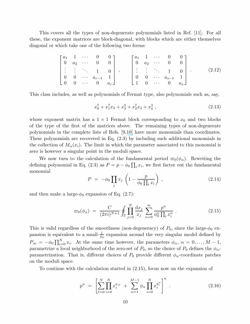
This covers all the types of non-degenerate polynomials listed in Ref. [11]. For all

these, the exponent matrices are block-diagonal, with blocks which are either themselves

diagonal or which take one of the following two forms:

a1 1 · · · 0 00 a2 · · · 0 0...

.... . . 1 0

0 0 · · · ar−1 10 0 · · · 0 ar

,

a1 1 · · · 0 00 a2 · · · 0 0...

.... . . 1 0

0 0 · · · as−1 11 0 · · · 0 as

. (2.12)

This class includes, as well as polynomials of Fermat type, also polynomials such as, say,

x70 + x7

1x3 + x33 + x7

2x4 + x34 , (2.13)

whose exponent matrix has a 1 × 1 Fermat block corresponding to x0 and two blocks

of the type of the first of the matrices above. The remaining types of non-degenerate

polynomials in the complete lists of Refs. [9,10] have more monomials than coordinates.

These polynomials are recovered in Eq. (2.3) by including such additional monomials in

the collection of Mα(xi). The limit in which the parameter associated to this monomial is

zero is however a singular point in the moduli space.

We now turn to the calculation of the fundamental period 0(φα). Rewriting the

defining polynomial in Eq. (2.3) as P = p− φ0

∏i xi, we first factor out the fundamental

monomial

P = −φ0

∏

j

xj

(1 − p

φ0

∏i xi

), (2.14)

and then make a large-φ0 expansion of Eq. (2.7):

0(φα) =C

(2πi)N+1

∮

Γ

N∏

j=0

dxjxj

∞∑

n=0

pn

φn0∏i x

ni

. (2.15)

This is valid regardless of the smoothness (non-degeneracy) of P0, since the large-φ0 ex-

pansion is equivalent to a small- 1φ0

expansion around the very singular model defined by

P∞ = −φ0

∏Ni=0 xi. At the same time however, the parameters φα, α = 0, . . . ,M − 1,

parametrize a local neighborhood of the zero-set of P0, so the choice of P0 defines the φα-

parametrization. That is, different choices of P0 provide different φα-coordinate patches

on the moduli space.

To continue with the calculation started in (2.15), focus now on the expansion of

pn =

[N∑

ℓ=0

N∏

i=0

xaiℓ

i +M−1∑

α=1

φα

N∏

i=0

xqα

i

i

]n. (2.16)

10

Using the multinomial formula,

( r∑

j=1

Xj

)n=

∑

ni∑ni=n

n!

n1!n2! · · ·nr!Xn1

1 Xn22 · · ·Xnr

r , (2.17)

one finds an explicit expression for pn,

pn =∑

ni,mα∑ℓnℓ+∑

αmα=n

( n!∏ni!∏mα!

) N∏

j=0

x(∑

ℓajℓnℓ+

∑αqα

j mα)

j

(M−1∏

α=1

φmαα

). (2.18)

Inserting (2.18) back into the expression (2.15) for 0(φα), each summand contains a

product of N+1 integrals

N∏

j=0

1

2πi

∮dxjxj

x(∑

ℓajℓnℓ+

∑αqα

j mα−n)

j . (2.19)

This N + 1-fold integral is nonzero precisely if the N + 1 relations

∑

ℓ

ajℓnℓ +∑

α

qαj mα = n , j = 0, . . . , N , (2.20)

are satisfied and each integral just picks out the residue at xi = 0. Multiplying (2.20)

by kj , summing over j = 0, . . . , N and using Eqs. (2.9), (2.11) and (2.1), we obtain∑i ni +

∑αmα = n , whence the condition imposed on nℓ, mα in the summations of

Eq. (2.18) is automatically satisfied for Calabi-Yau hypersurfaces. Thus we find that the

fundamental period is then given by by the remarkably simple expression:

0(φα) =∑

ni,mα

Γ(n+1)∏α Γ(mα+1)

∏i Γ(ni+1)

∏M−1α=1 φα

mα

φn0(2.21)

where

n =∑

i

ni +∑

α

mα , (2.22)

and the sums over ni and mα are restricted by Eq. (2.20), which provides N+1 conditions

for N+M+1 unknowns ni, mα, n. We are left with M free summation variables. There

are of course a number of different ways of choosing which variables to sum over. In what

follows we will solve for the ni.

We now would like to rewrite the above expression for 0 in a form which realizes

mirror symmetry and which also will turn out to be useful for the analytic continuation

to small-φ0 and for obtaining the other periods. The crucial observation here is that

11

the summation variables ni and n can be easily eliminated in (2.21), through (2.20) and

(2.22). The ni and nmay be expressed in terms of the M independent summation variables

mα, α = 1, . . . ,M−1, and a new variable r by setting

n = dr + t·m , ni = kir + si·m ,

mα = pαmα (no sum over α) ,(2.23)

where the dot-product denotes summation over α = 1, . . . ,M−1 and where the coefficients

d, ki, tα and si

α satisfy

N∑

j=0

kjaij = d , for each i , (2.24)

N∑

j=0

aijsjα + qαi p

α = tα , for each i and each α, (2.25)

for the constraints (2.20) to hold. Note also that (2.22) implies

d =N∑

i=0

ki and tα =N∑

i=0

siα + pα . (2.26)

Also, Eqs. (2.23) imply that the new variable r and the quantities t·m and si·m, for all

i, are integers. The pα are chosen so that all tα and sαi , and if possible also all mα,

are integers; we do not know if this is always possible, but have not been able to find a

counterexample.

From these relations we have that

N∑

j=0

(aij − 1)sjα = pα(1 − qαi ) , for each i and each α. (2.27)

Finally, with the above choice of aij , diagonal or as in (2.12), the matrix [aij − 1] is

invertible in general7 and the system of equations (2.27) can be solved for siα in terms of

pα, qαi and aij . The pα may then be chosen so as to obtain integral siα’s. Thereafter, the

tα are determined through (2.26). As promised, Eqs. (2.23) then eliminate the N+1 ni’s

and replace n by r, leaving M summation variables r, mα, α = 1, . . . ,M−1.

With these substitutions, the expression for the fundamental period (2.21) becomes

0(φ0, φα) =∑

r,mα

Γ(dr+1+∑α t

αmα)∏Ni=0 Γ(kir+1+

∑α si

αmα)

1

φdr0

M−1∏

α=1

ϕαmα

(pαmα)!; (2.28)

7 Amusingly, [aij−1] does have one vanishing eigenvalue for IP4[5], owing to ki = 1, which

means that the sαi can be determined only up to a scaling factor per each α—which still suffices

our present need.

12

here and hereafter, we drop the tilde over the m’s. We have also defined the new variables

ϕαdef= (φ p

α

α /φtα

0 ) . (2.29)

Equation (2.28) is the main result of this section. It gives an explicit form of the

fundamental period for all models defined as transverse hypersurfaces in weighted IP4,

once we have solved equations (2.24) and (2.25) for the coefficients d, ki, tα and sαi . This

is straightforward in all the cases. Most remarkably, upon rewriting the condition (2.24)

as∑j kja

Tji = d , comparison with Eq. (2.9) makes it clear that the ki are the weights

associated to the transposed polynomial PT0 of degree d that is used to construct the mirror

manifold in the class of models of Ref. [11].

We now illustrate this for the subclass of Fermat hypersurfaces. In this case the matrix

aij is diagonal aij = δijd/ki and d = d, ki = ki. The independent summation variables

are mα and r. We find, sαi = ki(tα − qαi p

α)/d and (2.23) become

n = d r +Q, ni = r ki +kid

(Q−Qi) , (2.30)

where Q ≡ m · tα, Qi ≡ pm · qi. The period then becomes

0(φ0, ϕα) =∑

r,mα

(dr+Q)!∏α ϕ

mαα∏N

j=0

(rkj+

kj

d(Q−Qj)

)!∏α(pαmα! (φ0)dr

. (2.31)

The case of a single modulus corresponds to setting M = 0 or equivalently mα = 0 in

Eq. (2.28). In this situation we find that Eq. (2.28) simplifies further to

0(φ0) =∑

r

Γ(dr + 1)∏j Γ(kjr + 1)φdr0

. (2.32)

This agrees with Batyrev’s results obtained by means of toric geometry [22]. It is also in

agreement with earlier studies restricted to one-modulus models [3–6] and in particular

with the quintic discussed in the introduction. Also, from (2.31) we can reproduce the

periods for the two moduli Fermat examples studied in Ref. [7]. Applications of Eq. (2.28)

in the case of two-parameter models, including non-Fermat hypersurfaces, will be given in

Section 4.

2.3. Convergence and analytic continuation: small ϕα

As should be clear from the general expression (2.28), the large-φ0 series expansion of 0

will be of the form of a generalized hypergeometric series. The analytic continuation of

such series is studied by means of integral representations of Mellin–Barnes type [32,3].

For the cases we consider this provides the analytic continuation of the series (2.28) into

the small-φ0 regime.

13

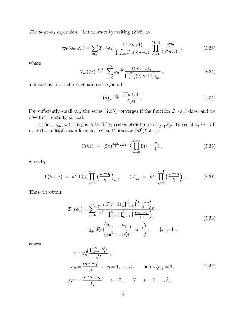
The large-φ0 expansion : Let us start by writing (2.28) as

0(φ0, ϕα) =∑

mα

Im(φ0)Γ(t·m+1)

∏Ni=0 Γ(si·m+1)

M−1∏

α=1

ϕmαα

(pαmα)!, (2.33)

where

Im(φ0)def=

∞∑

r=0

φ−dr0

(t·m+1)dr∏Ni=0(si·m+1)kir

, (2.34)

and we have used the Pochhammer’s symbol

(a)r

def=

Γ(a+r)

Γ(a). (2.35)

For sufficiently small ϕα, the series (2.33) converges if the function Im(φ0) does, and we

now turn to study Im(φ0).

In fact, Im(φ0) is a generalized hypergeometric function d+1Fd. To see this, we will

need the multiplication formula for the Γ-function [32](Vol. I):

Γ(kz) = (2π)1−k2 kkz−

12

k−1∏

q=0

Γ(z +q

k) , (2.36)

whereby

Γ(kr+z) = kkrΓ(z)k−1∏

q=0

(z + q

k

)

r,

(z)kr

= kkrk−1∏

q=0

(z + q

k

)

r. (2.37)

Thus, we obtain

Im(φ0) =

∞∑

r=0

z−r

r!

Γ(r+1)∏dp=1

(t·m+p

d

)

r∏Ni=0

∏ki

qi=1

(si·m+qi

ki

)

r

= d+1Fd

(a1, . . . , ad+1

c01, . . . , ckN

N

; z−1

), |z| > 1 ,

(2.38)

where

z = φ d0

∏Ni=0 k

ki

i

dd,

ap =t·m+ p

d, p = 1, . . . , d , and ad+1 = 1 ,

ciqi =

si·m+ qi

ki, i = 0, . . . , N, qi = 1, . . . , ki .

(2.39)

14

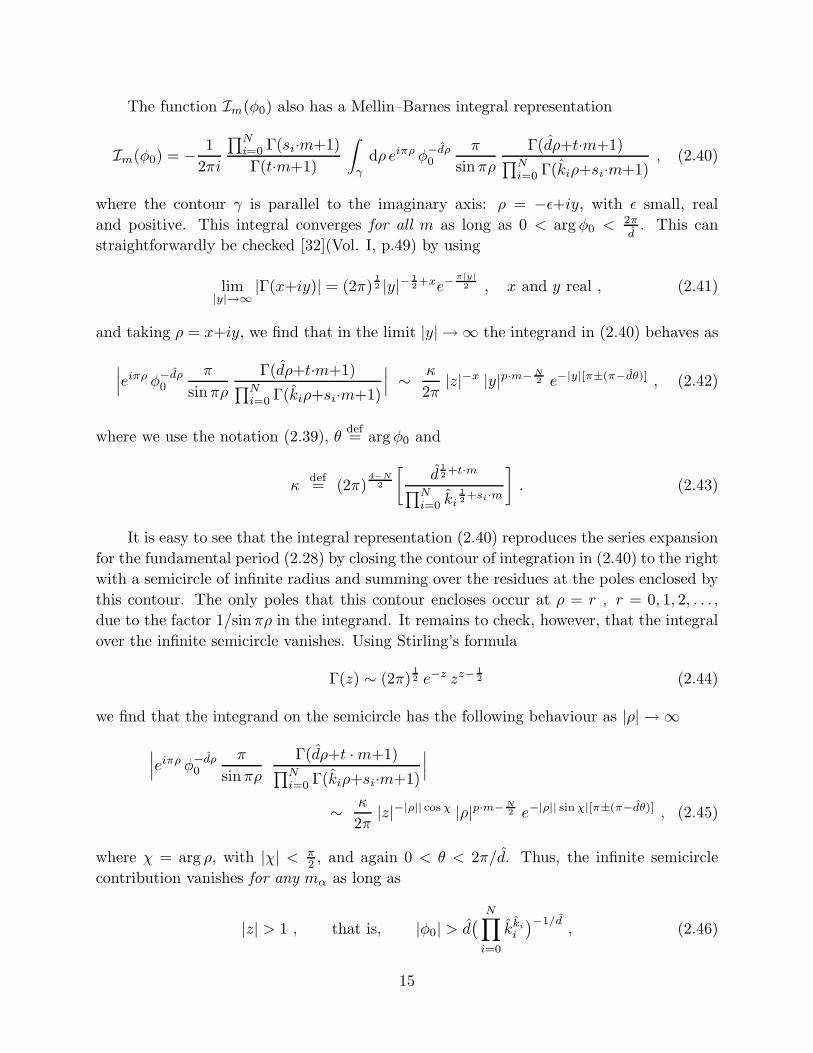
The function Im(φ0) also has a Mellin–Barnes integral representation

Im(φ0) = − 1

2πi

∏Ni=0 Γ(si·m+1)

Γ(t·m+1)

∫

γ

dρ eiπρ φ−dρ0

π

sinπρ

Γ(dρ+t·m+1)∏Ni=0 Γ(kiρ+si·m+1)

, (2.40)

where the contour γ is parallel to the imaginary axis: ρ = −ǫ+iy, with ǫ small, real

and positive. This integral converges for all m as long as 0 < arg φ0 < 2πd

. This can

straightforwardly be checked [32](Vol. I, p.49) by using

lim|y|→∞

|Γ(x+iy)| = (2π)12 |y|− 1

2+xe−π|y|2 , x and y real , (2.41)

and taking ρ = x+iy, we find that in the limit |y| → ∞ the integrand in (2.40) behaves as

∣∣∣eiπρ φ−dρ0

π

sinπρ

Γ(dρ+t·m+1)∏Ni=0 Γ(kiρ+si·m+1)

∣∣∣ ∼ κ

2π|z|−x |y|p·m−N

2 e−|y|[π±(π−dθ)] , (2.42)

where we use the notation (2.39), θdef= arg φ0 and

κdef= (2π)

4−N2

[d

12+t·m

∏Ni=0 ki

12+si·m

]. (2.43)

It is easy to see that the integral representation (2.40) reproduces the series expansion

for the fundamental period (2.28) by closing the contour of integration in (2.40) to the right

with a semicircle of infinite radius and summing over the residues at the poles enclosed by

this contour. The only poles that this contour encloses occur at ρ = r , r = 0, 1, 2, . . . ,

due to the factor 1/sinπρ in the integrand. It remains to check, however, that the integral

over the infinite semicircle vanishes. Using Stirling’s formula

Γ(z) ∼ (2π)12 e−z zz−

12 (2.44)

we find that the integrand on the semicircle has the following behaviour as |ρ| → ∞

∣∣∣eiπρ φ−dρ0

π

sinπρ

Γ(dρ+t ·m+1)∏Ni=0 Γ(kiρ+si·m+1)

∣∣∣

∼ κ

2π|z|−|ρ|| cosχ |ρ|p·m−N

2 e−|ρ|| sinχ|[π±(π−dθ)] , (2.45)

where χ = arg ρ, with |χ| < π2, and again 0 < θ < 2π/d. Thus, the infinite semicircle

contribution vanishes for any mα as long as

|z| > 1 , that is, |φ0| > d( N∏

i=0

kki

i

)−1/d, (2.46)

15

which is precisely the region of convergence of Im in (2.38).

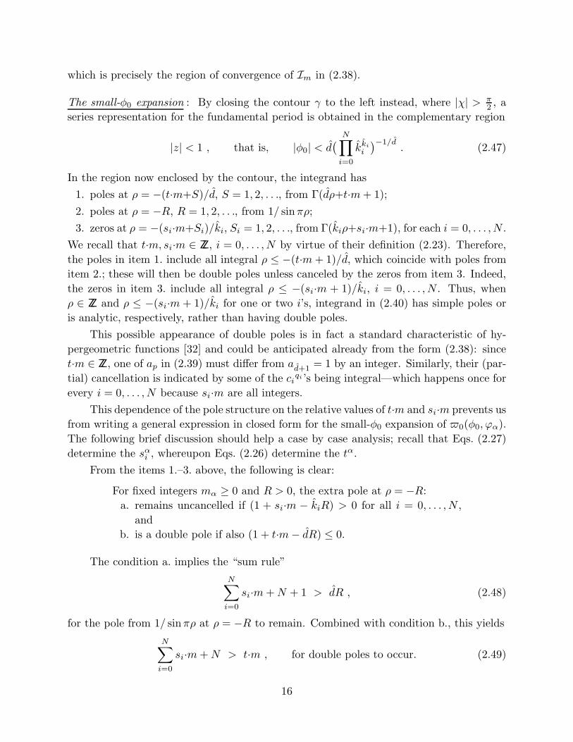
The small-φ0 expansion : By closing the contour γ to the left instead, where |χ| > π2 , a

series representation for the fundamental period is obtained in the complementary region

|z| < 1 , that is, |φ0| < d( N∏

i=0

kki

i

)−1/d. (2.47)

In the region now enclosed by the contour, the integrand has

1. poles at ρ = −(t·m+S)/d, S = 1, 2, . . ., from Γ(dρ+t·m+ 1);

2. poles at ρ = −R, R = 1, 2, . . ., from 1/ sinπρ;

3. zeros at ρ = −(si·m+Si)/ki, Si = 1, 2, . . ., from Γ(kiρ+si·m+1), for each i = 0, . . . , N .

We recall that t·m, si·m ∈ ZZ, i = 0, . . . , N by virtue of their definition (2.23). Therefore,

the poles in item 1. include all integral ρ ≤ −(t·m+ 1)/d, which coincide with poles from

item 2.; these will then be double poles unless canceled by the zeros from item 3. Indeed,

the zeros in item 3. include all integral ρ ≤ −(si·m + 1)/ki, i = 0, . . . , N . Thus, when

ρ ∈ ZZ and ρ ≤ −(si·m + 1)/ki for one or two i’s, integrand in (2.40) has simple poles or

is analytic, respectively, rather than having double poles.

This possible appearance of double poles is in fact a standard characteristic of hy-

pergeometric functions [32] and could be anticipated already from the form (2.38): since

t·m ∈ ZZ, one of ap in (2.39) must differ from ad+1 = 1 by an integer. Similarly, their (par-

tial) cancellation is indicated by some of the ciqi ’s being integral—which happens once for

every i = 0, . . . , N because si·m are all integers.

This dependence of the pole structure on the relative values of t·m and si·m prevents us

from writing a general expression in closed form for the small-φ0 expansion of 0(φ0, ϕα).

The following brief discussion should help a case by case analysis; recall that Eqs. (2.27)

determine the sαi , whereupon Eqs. (2.26) determine the tα.

From the items 1.–3. above, the following is clear:

For fixed integers mα ≥ 0 and R > 0, the extra pole at ρ = −R:

a. remains uncancelled if (1 + si·m − kiR) > 0 for all i = 0, . . . , N ,

and

b. is a double pole if also (1 + t·m− dR) ≤ 0.

The condition a. implies the “sum rule”

N∑

i=0

si·m+N + 1 > dR , (2.48)

for the pole from 1/ sinπρ at ρ = −R to remain. Combined with condition b., this yields

N∑

i=0

si·m+N > t·m , for double poles to occur. (2.49)

16

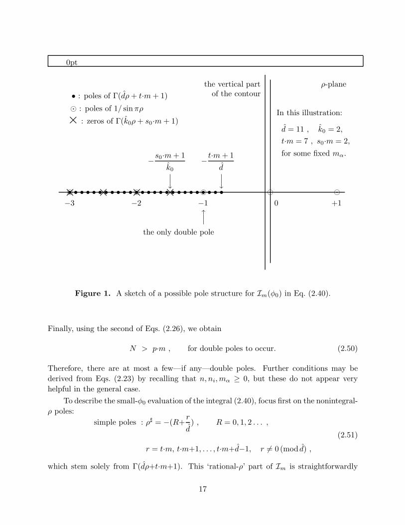
0pt

ρ-plane

In this illustration:

d = 11 , k0 = 2,

t·m = 7 , s0·m = 2,

for some fixed mα.

the vertical partof the contour• : poles of Γ(dρ+ t·m+ 1)

• • • • • • • • • • • • • • • • • • • • • • • • • •

y

− t·m+ 1

d

⊙ : poles of 1/ sinπρ

⊙−3

⊙−2

⊙−1x

the only double pole

⊙0

⊙+1

× : zeros of Γ(k0ρ+ s0·m+ 1)

× × × ×y

−s0·m+ 1

k0

Figure 1. A sketch of a possible pole structure for Im(φ0) in Eq. (2.40).

Finally, using the second of Eqs. (2.26), we obtain

N > p·m , for double poles to occur. (2.50)

Therefore, there are at most a few—if any—double poles. Further conditions may be

derived from Eqs. (2.23) by recalling that n, ni, mα ≥ 0, but these do not appear very

helpful in the general case.

To describe the small-φ0 evaluation of the integral (2.40), focus first on the nonintegral-

ρ poles:

simple poles : ρ♯ = −(R+r

d) , R = 0, 1, 2 . . . ,

r = t·m, t·m+1, . . . , t·m+d−1, r 6= 0(mod d) ,

(2.51)

which stem solely from Γ(dρ+t·m+1). This ‘rational-ρ’ part of Im is straightforwardly

17

obtained

I(Q)m (φ0) = −(−1)p·m

dπN

∏Ni=0 Γ(si·m+1)

Γ(t·m+1)

t·m+d−1∑

r=t·mr 6=0(mod d)

e−iπr

d

∏Nj=0 sin(

kjrπ

d)

sin(πrd

)(−φ0)

r

×∞∑

R=0

∏Nj=0 Γ(kj(R+ r

d)−sj·m)

Γ(dR+r−t·m)φdR0 .

(2.52)

Correspondingly,

(Q)0 = − 1

dπN

∑

mα

(−1)p·mt·m+d−1∑

r=t·mr 6=0(mod d)

e−iπr

d

∏Nj=0 sin(

kjrπ

d)

sin(πrd

)(−φ0)

r

×∞∑

R=0

∏Nj=0 Γ(kj(R+ r

d)−sj ·m)

Γ(dR+r−t·m)φdR0

M−1∏

α=1

ϕ mαα

(pαmα)!.

(2.53)

Now, to account for the possible integral-ρ poles, let

RDdef= −

[− t·m

d

], (2.54)

mark the onset of candidate double poles, where [x] denotes the largest integer not bigger

than x. Also, let R1 and R0, respectively, denote the smallest and the second-smallest

integer among−[− si·m

ki

]. These mark, respectively, the onset of the first and the second

band of zeros; for ρ ≤ −R0, all integral-ρ poles are canceled. Clearly, R0 ≥ R1. In addition,

assume that

−R0 ≤ −R1 ≤ −RD ≤ −1 , (2.55)

so that the integral-ρ residue contributions to (2.40) come from simple poles for −R0 <

ρ ≤ −R1 and −RD < ρ ≤ −1, but double poles for −R1 < ρ ≤ −RD. Straightforwardly

then, we can write

0(φ0, ϕα) = (Q)0 +

(Z)0 ,

(Z)0 =

(1)0 +

(2)0 +

(3)0 , (2.56)

18

with

(1)0 = −1

d

∑

mα

RD−1∑

R=1

Γ(1+t·m−dR)∏Nj=0 Γ(1+sj·m−kjR)

φdR0

M−1∏

α=1

ϕ mαα

(pαmα)!, (2.57)

(2)0 = −1

d

∑

mα

R1−1∑

R=RD

(−1)t·m+1(−φ0)dR

Γ(dR − t ·m)∏Nj=0 Γ(1+sj ·m−kjR)

M−1∏

α=1

ϕ mαα

(pαmα)!

×[ln[−φ−d0 ] + dΨ(dR−t·m) −

N∑

j=0

kjΨ(−kjR+sj·m+1)], (2.58)

(3)0 = −1

d

∑

mα

R0−1∑

R=R1

Γ(1+t·m−dR)∏Nj=0 Γ(1+sj ·m−kjR)

φdR0

M−1∏

α=1

ϕ mαα

(pαmα)!, (2.59)

where Ψ(z) is the logarithmic derivative of the Γ-function, and (Q)0 was given in (2.53).

Clearly, sums with an inverted range equal zero. For example, if R1 = R0, then (3)0 = 0.

When there is only one parameter the formula is very simple since, in this case, there

are no poles at all at ρ = −R. We obtain[33]

0(φ0) = − 1

dπN

d−1∑

r=1

e−πir

d (−φ0)r

∏Nj=0 sin

kjrπ

d

sin rπd

∞∑

R=0

φdR0

∏Nj=0 Γ

(kj(R+ r

d

))

Γ(dR+r), (2.60)

Using Eqs. (2.37), this can now be written in terms of a sum of generalized hypergeometric

functions dFd−1. We obtain [33]

0(φ0) = − 1

dπN

d−1∑

r=1

e−πir

d (−φ0)r

∏Nj=0 sin

kjrπ

dΓ(kjr

d

)

sin rπd

Γ(r)

× dFd−1

(N+1 times︷ ︸︸ ︷r

d, . . . , r

d, a1

0, . . . , akN−1N

r+1d, r+2

d. . . , r+d−1

d

; z

),

(2.61)

where

aqi

i =

(r

d+qi

ki

), i = 0, . . . , N , qi = 0, . . . , ki−1 . (2.62)

So far, through (2.40), we are able to find a series representation for the fundamental

period for any value of the modulus φ0. The series converges for sufficiently small values of

the remaining moduli ϕα. The radius of convergence however, is determined by the values

of these parameters for which the Calabi–Yau manifold becomes singular. It is difficult to

provide any detail about this in general and precise information seems to require study on

a case by case basis.

19

2.4. Convergence and analytic continuation: general ϕα

Looking back at Eq. (2.33), it is clear that 0(φ0, ϕα) will converge for small ϕα if Im(φ0)

does not grow too fast as a function of mα. For particular cases, it may be even possible

to use known results on the behaviour of generalized hypergeometric functions on their

parameters. In general, however, this approach does not seem to be fruitful.

We thus rewrite the fundamental period as

0 =∑

r

φ−dr0

r!

Γ(r+1)Γ(dr+1)∏Ni=0 Γ(kir+1)

Wr(ϕ) , (2.63)

where

Wr(ϕ) =∑

mα

(dr+1)t·m∏Ni=0(kir+1)si·m

∏

α

ϕmαα

(pαmα)!. (2.64)

The Mellin–Barnes integral representation of this is

0 = − 1

2πi

∫

γ

dρ φ−dρ0 eiπρπ

sinπρΓ(dρ+1)

Wρ(ϕ)∏Ni=0 Γ(kiρ+1)

, (2.65)

where the contour γ is chosen as before, parallel to the imaginary axis: ρ = −ǫ+iy, with ǫ

small, real and positive. In view of the previous analysis, this integral converges for small

ϕα as long as 0 < arg φ0 <2πd

.

The pole structure of the integrand in (2.65) is of course the same as the one in (2.40).

For ℜe(ρ) > −ǫ, the only poles stem from 1/ sinπρ and are located at ρ = r, r = 0, 1, 2, . . ..

For ρ = −1,−2, . . ., the poles stem both from Γ(dρ+1) and from 1/ sinπρ, and are double

poles unless canceled by the zeros of Wρ/∏i Γ(kir+1). For ρ = −(dR+r), with R =

0, 1, . . . and r = 1, 2, . . . , (d−1), Γ(dρ+1) has single poles. Indeed, although Wρ does have

poles, the function Wρ/∏i Γ(kir+1) has no poles whatsoever. This is easy to see from

the fact that the Pochhammer symbol (a)n has no poles for n > 0 and vanishes when

a = 0,−1,−2, . . . but also n+a > 0. Straightforwardly:

zeros ofWρ∏

i Γ(kir+1):

ρ = −(Z+1)/d Z = 0, 1, 2, . . . , (t·m−1),

ρ = −(Zi+si·m+1)/ki Zi = 0, 1, 2, . . . ,(2.66)

whence the same pole structure is recovered as in (2.40).

Recall that the discussion in the previous section was done for small ϕα; in fact to

zeroth order in ϕα. In particular, the radius of convergence only gives a condition on

φ0 which does not depend on the ϕα. In order to find the radius of convergence of the

Mellin-Barnes integral for general ϕα we need to know the asymptotic behaviour of |Wρ|as |ρ| → ∞; to close the integral in (2.65) to the left or right we have to make sure that

the integral over the semicircle vanishes as the radius goes to infinity.

20

Unfortunately, it is difficult to determine the asymptotic behaviour of Wρ(ϕ) as |ρ| →∞. We note however that the second formula in (2.37), combined with iterates of the

identity

(a)m+n = (a+m)n (a)m , (2.67)

allow the representation of Wρ(ϕ) as

Wρ(ϕα) =∑

mα

M−1∏

α=1

tα−1∏

ℓα=0

( dr+1+∑α−1β=1 t

βmβ+ℓα

tα

)

mα

sαi −1∏

ℓα=0

N∏

i=0

( kir+1+∑α−1β=1 s

βimβ+ℓα

sαi

)

mα

1pα−1∏

lα=1

(lαpα

)

mα

ζ mαα

mα!, (2.68)

where

ζαdef=

(tα)tα

ϕα

(pα)pα∏Ni=0(s

αi )s

αi

(2.69)

are suitably rescaled variables. The admittedly bewildering representation (2.68) of Wρ(ϕ)

however has the virtue of making it clear that Wρ(ϕ) is a multiple generalized hyperge-

ometric function. The standard techniques [Luke, I:VII] [34] may thus be developed to

study the asymptotic behaviour of Wρ(ϕ) as |ρ| → ∞, but this is beyond our present

scope. Here, we simply assume that the relevant integrals do converge and forego de-

termining the general, ϕα-dependent radii of convergence for the large-φ0 and small-φ0

expansions.

There being only simple poles at ρ = r = 0, 1, 2, . . .when the contour in (2.65) is closed

to the right, it is straightforward to verify that the integral representation of 0(φ0, ϕα)

indeed reproduces the small-φ0 expansion (2.63).

As for Im(φ0), the evaluation by residues of 0 in (2.65) may be separated into sums

over nonintegral-ρ:

simple poles : ρ♯ = −(R+r

d) , R = 0, 1, 2 . . . , r = 1, 2, . . . , d−1 , (2.70)

and integral-ρ residues. The latter are again finite in number and contain a possible

interval of double poles, as indicated in (2.55). The parametrization (2.70) clearly avoids

integral-ρ, but unlike in (2.51), does not manifest that the poles are canceled out down to

ρ = −(t·m)/d by the zeros (2.66). In this representation, we have

(Q)0 = − 1

dπN

d−1∑

r=1

e−iπr

d

∏Nj=0 sin(

kjrπ

d)

sin(πrd

)(−φ0)

r

×∞∑

R=0

∏Nj=0 Γ(kj(R+ r

d))

Γ(dR+r)φdR0 W−(R+ r

d)(ϕ) , (2.71)

21

(1)0 = −1

d

RD−1∑

R=1

[Γ(1−dR) W−R(ϕ)∏Nj=0 Γ(1−kjR)

]φdR0 , (2.72)

(2)0 = +

1

d

R1−1∑

R=RD

W−R(ϕ) (−φ0)dR

Γ(dR)∏Nj=0 Γ(1−kjR)

×[ln[−φ−d0 ] + dΨ(dR) −

N∑

j=0

kjΨ(1 − kjR) + w−R(ϕ)], (2.73)

(3)0 = −1

d

R0−1∑

R=R1

[Γ(1−dR) W−R(ϕ)∏Nj=0 Γ(1−kjR)

]φdR0 , (2.74)

where

wρ(ϕ)def=

1

Wρ(ϕ)

d

dρWρ(ϕ) .

Despite appearances, the quantities in square brackets in (2.72) and (2.74) are finite owing

to the zeros (2.66).

2.5. The remaining periods

The analytic continuation of the fundamental period obtained from (2.40) very often suf-

fices to find the other periods. Let M denote the zero set of the defining polynomial (2.3).

The φα, α = 0, . . . ,M−1 parametrize the space of complex structures for M centered

around the reference polynomial P0. This reference manifold typically enjoys some sym-

metries and those which act diagonally on the coordinates play a special role [12]; denote

them by GM. Clearly, any two deformations of the reference manifold which are related

by a GM transformation must be identified. Thus, there is a (lifted) action, A, of GM

on the parameter space, the proper moduli space must be (at least) an A-quotient of the

parameter space and the point represented by P0 becomes an A-orbifold point. Although

the full modular group is in general not known, A is clearly at least a subgroup and acts

on the parameter space

A : φα 7−→ λai

α

i φα α = 0, 1, . . . ,M−1, λd = 1, i = 1, . . . , r , (2.75)

where A ∼ ZZd1 × . . . × ZZdr. In particular we have d1 = d where d is the degree of the

transposed polynomial, a quotient of which gives the mirror W of M. We then define the

set of periods j1...jr as

j1...jr(φα)def= 0(λ

j a1α

1 φα, . . . , λj ar

αr φα) . (2.76)

22

Assume first that (Z)0 = 0; that is, only residues at nonintegral-ρ contribute to the

small-φ0 expansion of 0. Since (Q)0 does not contain d’th powers of φ0, it follows that

d∑

j=1

(Q)0 (λj1φ0, ϕα) =

d∑

j=1

0(λj1φ0, ϕα) = 0 . (2.77)

Thus, at most (∑i di)−1 of the

∑i di periods are linearly independent. However, if at least

one of (1)0 ,

(3)0 is also nonzero, this no longer holds. Clearly,

(1)0 and

(3)0 are functions

of φd0, rather than φ0 and are consequently invariant under the ZZd action φ0 7→ λ1φ0, with

λd1 = 1. Thend∑

j=1

0(λj1φ0, ϕα) = d(

(1)0 +

(3)0 ) 6= 0 . (2.78)

Finally, because of the logarithmic term in (2.58) and (2.73), the presence of (2)0 6= 0,

i.e. the contribution of double poles in (2.40) and (2.65), would change the behaviour of

0(φ0, ϕα) substantially.

We again assume that (Z)0 = 0, so that 0 =

(Q)0 . Given the explicit factors of

sin(kjrπ

d) in Eqs. (2.53) and (2.71), it should be clear that the terms with kjr = 0(mod d)

are also absent. This implies additional conditions on the periods, corresponding to a

modular group action

(φ0, φα) 7−→ (λkjφ0, λkjt

α

φα) . (2.79)

Of course, further relations may exist in specific models owing to accidental cancellations.

With this we can now obtain a collection of complex structure periods j for general

Calabi-Yau hypersurfaces in weighted projective spaces and so also for the corresponding

Landau-Ginzburg models. The action of A in Eq. (2.76) produces a complete set of such

periods for all models described above. This provides a basis for a complete description

of the special geometry of the space of complex structures for these models, and also the

spaces of (complexified) Kahler classes for their mirror models. In the subsequent sections,

we will attempt various generalizations of these results.

23

3. CICY Manifolds

We now turn to the calculation of the Kahler class periods for some simple models. One

difficulty here will be the identification of suitable parameters and mirror symmetry will

be found most useful.

3.1. Complete intersections in a single projective space

We will compute here the periods for the Kahler class parameters for the five families of

manifolds: IP4[5], IP5[3, 3], IP5[2, 4], IP6[2, 2, 3] and IP7[2, 2, 2, 2]. Let us begin with the

manifold IP5[3,3]. Libgober and Teitelbaum [21] seem to have correctly guessed the mirror

of this manifold by considering the one parameter family, Mψ, of IP5[3, 3] manifolds given

by the polynomialsp1 = x3

0 + x31 + x3

2 − 3ψ x3x4x5 ,

p2 = x33 + x3

4 + x35 − 3ψ x0x1x2 .

(3.1)

Libgober and Teitelbaum observe that (i) there is a group of phase symmetries H such that

these polynomials are in fact the most general polynomials whose zero locus is invariant

under H. (ii) The manifold obtained by resolving Mψ/H has the values of b1,1 and b2,1exchanged relative to IP5[3, 3]. Moreover, (iii) the numbers, nk, of instantons of degree k

inferred by calculating the Yukawa coupling yields the correct number in degree one and

integral values for all k (the number of instantons has been checked also in degree two).

Underlying much of the present work is the important fact that the holomorphic three-

form may be realised as a residue where the manifold of interest is a submanifold in a space

of higher dimension. For the manifolds of this section, which are given by N transverse

polynomials pα, α = 1, . . . , N in IPN+3, the holomorphic three form can be written as a

residue of the (N + 3)-form

ǫA1A2···AN+4 xA1dxA2

· · ·dxAN+4

p1 p2 · · · pN, (3.2)

which is integrated around N circles that enclose the loci pα = 0. Let deg(α) denote the

degree of pα and note that both the numerator and denominator of the N + 3-form scale

the same way under xA → λxA in virtue of the Calabi–Yau condition

N∑

α=1

deg(α) = N + 4 . (3.3)

In view of the above discussion, we may define a fundamental cycle B0 for the mirror

of IP5[3, 3] in analogy with (1.5). We therefore arrive at the following expression for the

24

fundamental period that is the analogue of (1.7)

0 =1

(2πi)6

∮

γ0×···×γ5

(3ψ)2 dx0 · · ·dx5

p1 p2. (3.4)

By extracting a factor of x0 · · ·x5 from the denominator and expanding in inverse powers

of ψ we have

0 =1

(2πi)6

∫dx0 · · ·dx5

x0 · · ·x5

∞∑

k=0

[x3

0 + x31 + x3

2

]k

(3ψx3x4x5)k

∞∑

l=0

[x3

3 + x34 + x3

5

]l

(3ψx0x1x2)l. (3.5)

As in the case of the quintic the only terms that contribute are the terms in the sums that

are independent of the xA. Such terms arise in the product only when k = l = 3n and the

contribution is then(

(3n)!(n!)3

)2

. Thus, we find

0 =∞∑

n=0

((3n)!)2

(n!)6 (3ψ)6n= 4F3

(13,2

3,1

3,2

3; 1, 1, 1;ψ−6

). (3.6)

For the remaining manifolds the computations are analogous. The fundamental period is

given by the expression

0 =

∏Nα=1

(−deg(α)ψ

)

(2πi)N+4

∫

γ1×···×γN+4

dx1 · · ·dxN+4

p1 · · · pN. (3.7)

The polynomials together with the resulting periods are displayed in Table 3.1

One finds that the periods of Table 3.1 may be related to standard functions by means

of the multiplication formula (2.36). We obtain in this way that the periods are given by

generalized hypergeometric functions pFq. Recall that these are defined by the series

pFq

(a1, . . . , apc1, . . . , cq

; z)

=

∞∑

k=0

(a1)k, . . . , (ap)k(c1)k, . . . , (cq)k

zk

k!, (3.8)

where (a)r is the Pochhammer’s symbol (see Eq. (2.35)). In fact, the periods of Table 3.1

are all of the form

4F3

(a1, . . . , a4

1, 1, 1; (Cψ)−d

)(3.9)

with the a-indices (a1, a2, a3, a4) taking the values shown in the last column of Table 3.1.

We see that each polynomial of degree d contributes the indices 1d ,

2d , · · · , d−1

d .

We will turn now to the analytic continuation for the fundamental periods of these

models. We will mostly concentrate on IP5[3, 3] to illustrate the procedure since it is

analogous for the other cases. The method is essentially the same as for IP4[5] [3].

25

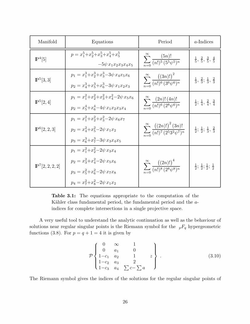
Manifold Equations Period a-Indices

IP4[5]p = x5

1+x52+x

53+x

54+x

55

−5ψx1x2x3x4x5

∞∑

n=0

(5n)!

(n!)5 (55ψ5)n15 ,

25 ,

35 ,

45

IP5[3, 3]p1 = x3

1+x32+x

33−3ψx4x5x6

p2 = x34+x

35+x

36−3ψx1x2x3

∞∑

n=0

((3n)!

)2

(n!)6 (36ψ6)n13 ,

23 ; 1

3 ,23

IP5[2, 4]p1 = x2

1+x22+x

23+x

24−2ψx5x6

p2 = x45+x

46−4ψ x1x2x3x4

∞∑

n=0

(2n)! (4n)!

(n!)6 (28ψ6)n12; 1

4, 2

4, 3

4

IP6[2, 2, 3]

p1 = x21+x

22+x

23−2ψx6x7

p2 = x24+x

25−2ψ x1x2

p3 = x36+x

37−3ψ x3x4x5

∞∑

n=0

((2n)!

)2(3n)!

(n!)7 (2532ψ7)n12; 1

2; 1

3, 2

3

IP7[2, 2, 2, 2]

p1 = x21+x

22−2ψ x3x4

p2 = x23+x

24−2ψ x5x6

p3 = x25+x

26−2ψ x7x8

p4 = x27+x

28−2ψ x1x2

∞∑

n=0

((2n)!

)4

(n!)8 (28ψ8)n12; 1

2; 1

2; 1

2

Table 3.1: The equations appropriate to the computation of the

Kahler class fundamental period, the fundamental period and the a-

indices for complete intersections in a single projective space.

A very useful tool to understand the analytic continuation as well as the behaviour of

solutions near regular singular points is the Riemann symbol for the pFq hypergeometric

functions (3.8). For p = q + 1 = 4 it is given by

P

0 ∞ 10 a1 0

1−c1 a2 1 z1−c2 a3 21−c3 a4

∑c−∑a

. (3.10)

The Riemann symbol gives the indices of the solutions for the regular singular points of

26

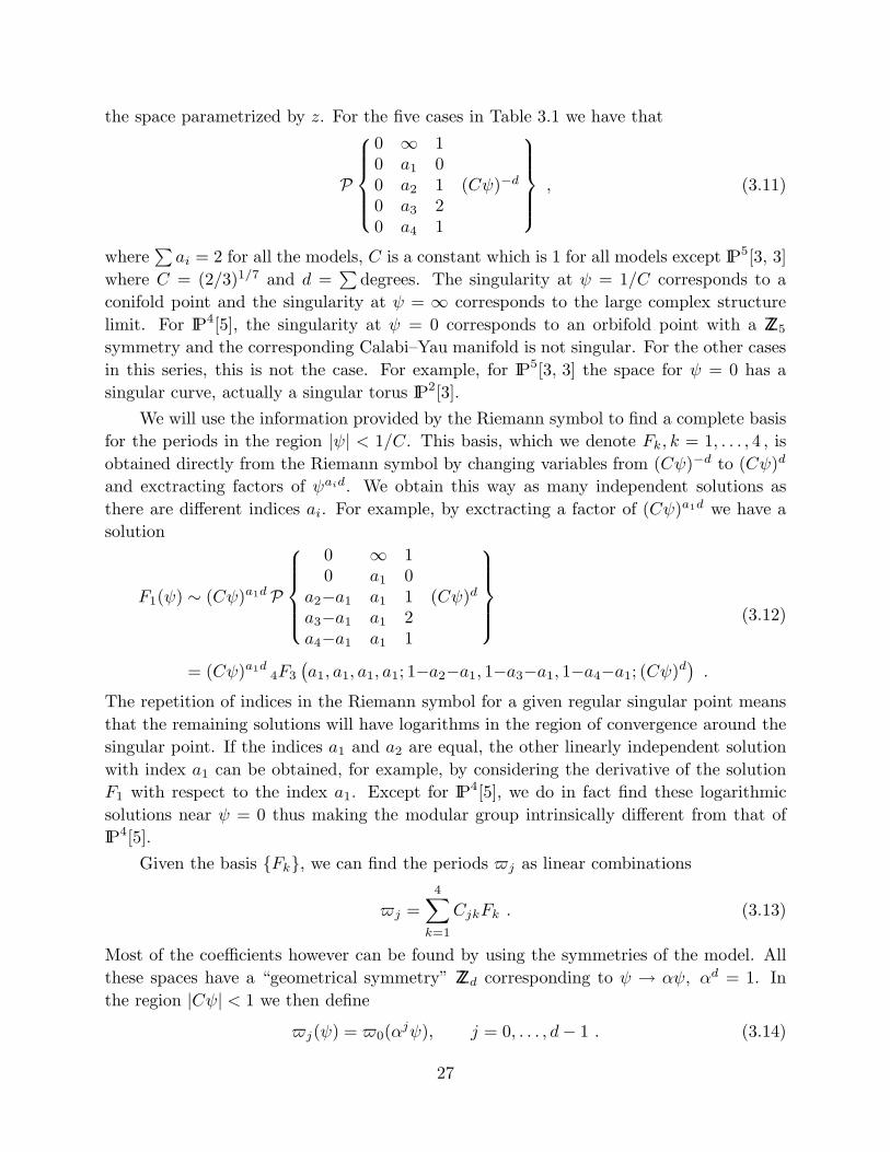
the space parametrized by z. For the five cases in Table 3.1 we have that

P

0 ∞ 10 a1 00 a2 1 (Cψ)−d

0 a3 20 a4 1

, (3.11)

where∑ai = 2 for all the models, C is a constant which is 1 for all models except IP5[3, 3]

where C = (2/3)1/7 and d =∑

degrees. The singularity at ψ = 1/C corresponds to a

conifold point and the singularity at ψ = ∞ corresponds to the large complex structure

limit. For IP4[5], the singularity at ψ = 0 corresponds to an orbifold point with a ZZ5

symmetry and the corresponding Calabi–Yau manifold is not singular. For the other cases

in this series, this is not the case. For example, for IP5[3, 3] the space for ψ = 0 has a

singular curve, actually a singular torus IP2[3].

We will use the information provided by the Riemann symbol to find a complete basis

for the periods in the region |ψ| < 1/C. This basis, which we denote Fk, k = 1, . . . , 4 , is

obtained directly from the Riemann symbol by changing variables from (Cψ)−d to (Cψ)d

and exctracting factors of ψaid. We obtain this way as many independent solutions as

there are different indices ai. For example, by exctracting a factor of (Cψ)a1d we have a

solution

F1(ψ) ∼ (Cψ)a1dP

0 ∞ 10 a1 0

a2−a1 a1 1 (Cψ)d

a3−a1 a1 2a4−a1 a1 1

= (Cψ)a1d4F3

(a1, a1, a1, a1; 1−a2−a1, 1−a3−a1, 1−a4−a1; (Cψ)d

).

(3.12)

The repetition of indices in the Riemann symbol for a given regular singular point means

that the remaining solutions will have logarithms in the region of convergence around the

singular point. If the indices a1 and a2 are equal, the other linearly independent solution

with index a1 can be obtained, for example, by considering the derivative of the solution

F1 with respect to the index a1. Except for IP4[5], we do in fact find these logarithmic

solutions near ψ = 0 thus making the modular group intrinsically different from that of

IP4[5].

Given the basis Fk, we can find the periods j as linear combinations

j =

4∑

k=1

CjkFk . (3.13)

Most of the coefficients however can be found by using the symmetries of the model. All

these spaces have a “geometrical symmetry” ZZd corresponding to ψ → αψ, αd = 1. In

the region |Cψ| < 1 we then define

j(ψ) = 0(αjψ), j = 0, . . . , d− 1 . (3.14)

27

There are, of course, linear relations between these periods since only four of them are

linearly independent. Equation (3.14) determines Cjk, for all j 6= 0. The coefficients C0k

can be found from the analytic continuation of the period 0 for |Cψ| > 1 to the region

|Cψ| < 1. The periods j(ψ) in the region |Cψ| > 1 can also be obtained by analytic

continuation to this region of the representations in (3.13) for |Cψ| < 1.

Consider now IP5[3, 3]; there will be two solutions with logarithms in the region |ψ| < 1

(with C = 1). The solutions without logarithms are

Fk(ψ) = (3ψ)2kΓ(k

3)4

Γ(k)24F3

k3,k

3,k

3,k

3;

︷ ︸︸ ︷k+1

3,k+2

3,k+1

3,k+2

3;ψ6

,

= (3ψ)2k∞∑

n=0

(3ψ)6nΓ6(n+k

3 )

Γ2(3n+k), k = 1, 2 ,

(3.15)

where the overbrace means that an index that is equal to 1 must be deleted. The other

two linearly independent solutions can be chosen so that

Fk+2(ψ) =d

dkFk(ψ)

= log(3ψ)2 Fk

+ 2(3ψ)2k∞∑

n=0

(3ψ)6nΓ6(n+k

3)

Γ2(3n+k)

[Ψ

(n+

k

3

)− Ψ(3n+k)

], k = 1, 2 .

(3.16)

Let

0(ψ) =2∑

k=1

(CkFk + Ck+2Fk+2) . (3.17)

Since this theory has a geometrical symmetry ZZ6, we define

j(ψ) = 0(αjψ) , α6 = 1 , (3.18)

where not all six j(ψ) are linearly independent. We obtain

j(ψ) =2∑

k=1

α2kj

[(Ck +

2πi

3j Ck+2

)Fk + Ck+2Fk+2

], (3.19)

sinceFk(α

jψ) = α2kj Fk(ψ) ,

Fk+2(αjψ) = α2kj

[Fk+2(ψ) +

2πi

3j Fk(ψ)

], k = 1, 2 .

(3.20)

28

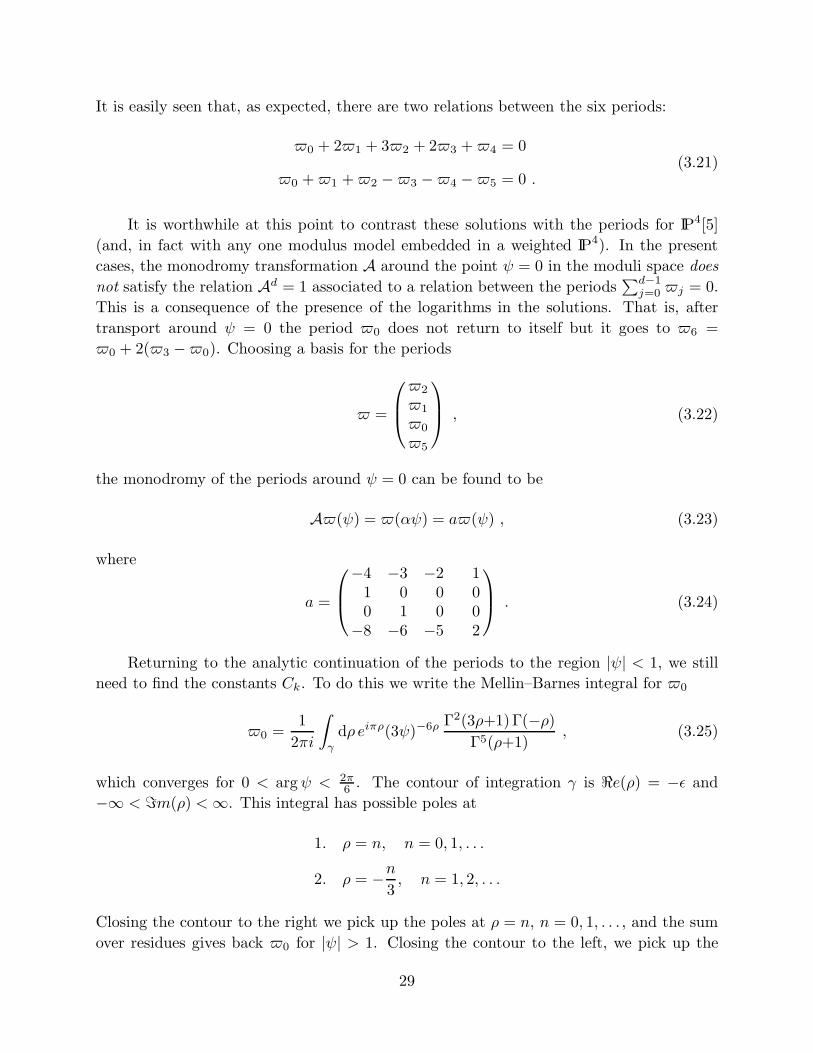
It is easily seen that, as expected, there are two relations between the six periods:

0 + 21 + 32 + 23 +4 = 0

0 +1 +2 −3 −4 −5 = 0 .(3.21)

It is worthwhile at this point to contrast these solutions with the periods for IP4[5]

(and, in fact with any one modulus model embedded in a weighted IP4). In the present

cases, the monodromy transformation A around the point ψ = 0 in the moduli space does

not satisfy the relation Ad = 1 associated to a relation between the periods∑d−1j=0 j = 0.

This is a consequence of the presence of the logarithms in the solutions. That is, after

transport around ψ = 0 the period 0 does not return to itself but it goes to 6 =

0 + 2(3 −0). Choosing a basis for the periods

=

2

1

0

5

, (3.22)

the monodromy of the periods around ψ = 0 can be found to be

A(ψ) = (αψ) = a(ψ) , (3.23)

where

a =

−4 −3 −2 11 0 0 00 1 0 0

−8 −6 −5 2

. (3.24)

Returning to the analytic continuation of the periods to the region |ψ| < 1, we still

need to find the constants Ck. To do this we write the Mellin–Barnes integral for 0

0 =1

2πi

∫

γ

dρ eiπρ(3ψ)−6ρ Γ2(3ρ+1)Γ(−ρ)Γ5(ρ+1)

, (3.25)

which converges for 0 < argψ < 2π6 . The contour of integration γ is ℜe(ρ) = −ǫ and

−∞ < ℑm(ρ) <∞. This integral has possible poles at

1. ρ = n, n = 0, 1, . . .

2. ρ = −n3, n = 1, 2, . . .

Closing the contour to the right we pick up the poles at ρ = n, n = 0, 1, . . . , and the sum

over residues gives back 0 for |ψ| > 1. Closing the contour to the left, we pick up the

29

poles at ρ = −n3 , n = 1, 2, . . ., which are actually double poles. We obtain

0 =1

9

∞∑

n=1

(3ψ)2nα−n Γ(n3 )

Γ2(n)Γ5(1−n3 )

log[−(3ψ)−6] − Ψ

(n3

)− 5Ψ

(1−n

3

)+ 6Ψ(n)

,

= − 332

(2π)5

2∑

k=1

α−k

[π

3

(−i+ 5 cot

kπ

3

)]Fk + Fk+2

, |ψ| < 1

(3.26)

Thus

Ck = − 312

25π4α−k

(−i+ 5 cot

kπ

3

),

Ck+2 = − 332

(2π)5α−k , k = 1, 2 ,

(3.27)

and

j(ψ) = − 332

(2π)5

2∑

k=1

αk(2j−1)

π

3

[(2j − 1)i+ 5 cot

kπ

3

]Fk + Fk+2

, |ψ| < 1 .

(3.28)

The reader may enjoy the straightforward exercise of finding the monodromy of the

periods around ψ = 1 and ψ = ∞. Following [3], the periods near ψ = 1 are given by

j = − cj2πi

(1 −0) log(ψ−1) + gj , (3.29)

with gj analytic for |ψ − 1| < 1 and where the constants cj are

(cj) = (1, 1,−5, 10,−8,−5) . (3.30)

The matrix t corresponding to the monodromy T about ψ = 1 is therefore

t =

1 5 −5 00 0 1 00 −1 2 00 5 −5 1

. (3.31)

The monodromy about ψ = ∞ can be easily obtained from the fact that a loop around all

the singularities (ψ = αj for j = 0, . . . , 5, ψ = 0 and ψ = ∞) is contractible:

1 = t∞(at)6 . (3.32)

Therefore

t−1∞ =

−4 −23 20 −11 5 −5 00 0 1 0

−8 −25 14 2

. (3.33)

30

A series representation for the periods in the region |ψ| > 1 can be similarly obtained

[3] by considering the following integral representation of Fk

Fk = −(3ψ)2k

2πi

∫

γ

ds eiπs (3ψ)6sπ

sinπs

Γ6(s+k3 )

Γ2(3s+k)k = 1, 2 , (3.34)

but here we will not pursue this matter any further.

As a final comment, we would like to remark that the space IP7[2, 2, 2, 2] is a little

different from the others in this series in the sense that its periods for small-ψ behave very

differently. The singularity at ψ = 0 is of the same type as the singularity at ψ = ∞and the reason behind this is that the moduli space for this model has an extra symmetry

ψ → 1/ψ.

3.2. Calabi-Yau hypersurfaces in products of projective spaces

Consider next the five families of CICY manifolds:

IP4[ 5 ] , IP2

IP2

[33

],

IP1

IP3

[24

],

IP1

IP1

IP2

223

,

IP1

IP1

IP1

IP1

2222

,

(3.35)

that are defined by a single polynomial. We wish to obtain the fundamental period for

their space of Kahler classes using mirror symmetry. Each family has one Kahler class

parameter for each IPn factor. The generalization of the analysis presented in Section 2 to

these models requires several choices pertaining to the identification of the deformations of

the complex structure mirroring the Kahler classes of each IPn factor of the ambient space.

We will return to discuss these below. However, for the five families of spaces (3.35) the

fundamental period may be found by applying the construction of Batyrev [22].

Consider for example the family of manifolds

IP2

IP2

[33

], (3.36)

and denote by (x0, x1, x2) and (y0, y1, y2) the homogeneous coordinates of the two IP2’s. We

restrict the coordinates to the set T on which no coordinate vanishes and take x0 = y0 = 1

so that (x1, x2; y1, y2) are affine coordinates on the embedding space. Let

f =p

x1x2y1y2=

∑

m1,m2;n1,n2

am1m2n1n2xm1

1 xm22 yn1

1 yn22 . (3.37)

The Newton polyhedron, ∆, of the manifold is the convex hull of the points (m1, m2;n1, n2)

for which the coefficients a of the Laurent polynomial f are nonzero. For this elementary

31

example these are the points for which

−1 ≤ m1 , −1 ≤ m2 ; −1 ≤ n1 , −1 ≤ n2

m1 +m2 ≤ 1 ; n1 + n2 ≤ 1 .

(3.38)

The vertices of the polyhedron dual to ∆ are the six points:

(1, 0, 0, 0) , (0, 1, 0, 0) , (0, 0, 1, 0) , (0, 0, 0, 1) ,

(−1,−1, 0, 0) , (0, 0,−1,−1) .(3.39)

These points are the coefficients in the inequalities (3.38) if the inequalities are replaced

by equalities and we multiply through if necessary so that the constant term is −1 in each

case. The Laurent polynomial corresponding to the dual polyhedron is

f = 1 +X1 +X2 +λ1

X1X2+ Y1 + Y2 +

λ2

Y1Y2(3.40)

where the freedom to make linear redefinitions of the coordinates and to multiply f by an

overall factor has been used to reduce the number of free parameters to two which is the

correct number since b1,1 = 2 for the original manifold (3.36).

We may now revert to homogeneous coordinates by setting X1 = x1

x0, X2 = x2

x0etc.

Then the mirror manifold is given by the singular bicubic hypersurface p = 0 in IP2 × IP2

with

p = X1X2Y1Y2f

= x0x1x2 y0y1y2 + (x21x2 + x1x

22 + λ1x

30) y0y1y2 + (y2

1y2 + y1y22 + λ2y

30)x0x1x2 .

(3.41)

The fundamental period for the mirror now follows in a manner that has become familiar:

0(λ1, λ2) =1

(2πi)6

∫dx0dx1dx2 dy0dy1dy2

p

=∞∑

n1,n2=0

(3n1 + 3n2)!

(n1!)3(n2!)3λn1

1 λn22 .

(3.42)

The other cases follow in precise analogy and we list the fundamental Kahler class periods in

Table 3.2 to reveal the pattern. These spaces would seem to furnish rather simple examples

of multiparameter spaces which might be easier to analyse than the multiparameter cases

studied thus far [4–7]. Note also that these spaces do not have a single ‘fundamental’

parameter; rather they have several, one corresponding to the Kahler class of each factor

space.

32

Manifold Period

IP4[ 5 ]

∞∑

n=0

(5n)!

(n!)5λn

IP2

IP2

[33

] ∞∑

n1,n2=0

(3n1 + 3n2)!

(n1!)3 (n2!)3λn1

1 λn22

IP1

IP3

[24

] ∞∑

n1,n2=0

(2n1 + 4n2)!

(n1!)2 (n2!)4λn1

1 λn22

IP1

IP1

IP2

223

∞∑

n1,n2,n3=0

(2n1 + 2n2 + 3n3)!

(n1!)2 (n2!)2 (n3!)3λn1

1 λn22 λn3

3

IP1

IP1

IP1

IP1

2222

∞∑

n1,n2,n3,n4=0

(2n1 + 2n2 + 2n3 + 2n4)!

(n1!)2 (n2!)2 (n3!)2 (n4!)2λn1

1 λn22 λn3

3 λn44

Table 3.2: The Kahler class fundamental periods for Calabi-Yau

hypersurfaces in products of projective spaces.

3.3. A natural conjecture

We now know the Kahler class for the fundamental periods for CICY manifolds for which

the degree matrix consists either of a single row or a single column. Based on this, it is

natural to conjecture a form for a general weighted CICY—with F > 1 factor spaces

IPn1

(k(1)1 ,...,k

(1)n1+1

)× · · · × IPnF

(k(F )1 ,...,k

(F)nF +1

), (3.43)

and N > 1 polynomials pα, α = 1, . . . , N such that the degree of pα in the variables of

the j’th projective space is degj(α) which, in order to have a Calabi–Yau manifold, they

must satisfy the relations

∑

α

degj(α) =

nj+1∑

i=1

k(j)i , for all j . (3.44)

33

The fundamental period is then given, as a function of the parameters λj corresponding

to the Kahler classes of each factor space, by

0(λ1, . . . , λF ) =

∞∑

m1,...,mF =0

∏Nα=1

(∑Fj=1 degj(α)mj

)!

(∏n1+1i=1 (k

(1)i m1)!

)· · ·(∏nF +1

i=1 (k(F )i mF )!

) λm11 · · ·λmF

F .

(3.45)

We illustrate this conjecture below. It is compatible with all other examples for which the

period has already been calculated [35,24].

By way of an example of this conjecture, consider the Schimmrigk manifold [23],

M ∈ IP3

IP2

[3 10 3

]:

p1,0(x) =

3∑

i=0

x3i

p2,0(x, y) =3∑

i=1

xiy3i

= 0 .

= 0 ,

(3.46)

Identify first x1x2x3 and x0y1y2y3 as the fundamental deformations of p10 and p2

0 respec-

tively. Thus, we want to find the periods associated to a deformation of M given by

p1 = p1,0 − ψ1x1x2x3 ,

p2 = p2,0 − ψ2x0y1y2y3 .(3.47)

Note that x1x2x3 and x0y1y2y3 are left invariant under action of the quotient symme-

try H which produces the mirror manifold, W = M/H. Therefore, by mirror symmetry,

the fundamental period may also be thought of as representing deformations of the Kahler

class of M. The period follows straightforwardly as in previous examples,

0 = (−ψ1)(−ψ2)1

(2πi)7

∮

Γ

dx0 . . .dy3p1 p2

, (3.48)

which becomes

0 =1

(2πi)7

∫

Γ

dx0 . . .dy3x0 . . . y3

∞∑

n=0

(x3

0 + . . .+ x33

ψ1x1x2x3

) ∞∑

m=0

(x1y

31 + . . .+ x3y

33

ψ2x0y1y2y3

)

=∞∑

m1,m2=0

(3m1)! (3m2 +m1)!

(m1!)4(m2!)31

(ψ1)3m2+m1(ψ2)3m1.

(3.49)

Indeed, upon identifying λ−11 = ψ1ψ

32 and λ−1

2 = ψ31 , this is seen to be the appropriate

special case of the conjecture (3.45). Note also that this is not the complete answer;

b1,1 = 8 for this CICY manifold while we have here obtained the fundamental period only

34

as a function of two moduli, the ones corresponding to the Kahler classes on IP3 and IP2.

The dependence on the remaining six parameters will be discussed in Section 5.

Another interesting example of the above is to consider the two-parameter (Fermat)

models which will be discussed in Section 4.1. For the first four models in (4.1) one

can (for specific values of the moduli) relate them to one-parameter families of complete

intersections in a weighted projective space. In particular, let us consider a two-parameter

deformation of IP4(1,1,2,2,6)[12]128,2−252 given by (4.2). From the discussion in Section 4.1 one

finds that the fundamental period may be written as

0 =

∞∑

l=0

Γ(6l + 1)

Γ3(l + 1)Γ(3l + 1)

( −1

(12ψ)6

)Ul(φ) (3.50)

where Ul(φ) is given by (4.7). At the singular curve φ = 1, Ul(φ = 1) = Γ(2l+1)Γ2(l+1)

, and hence

(3.50) becomes

0 =∑

l=0

∞Γ(6l + 1)Γ(2l + 1)

Γ5(l + 1)Γ(3l + 1)

( −1

(12ψ)6

)l. (3.51)

But according to the conjecture, Eq. (3.51) is the fundamental period for IP5(1,1,1,1,1,3)[6, 2].

Indeed, it can be shown[36] that this manifold is birational to IP4(1,1,2,2,6)[12].

35

4. Hypersurfaces with Two Parameters

4.1. Fermat hypersurfaces

For Fermat hypersurfaces it is possible to derive some general results from the explicit

form of the fundamental period given in (2.28). There are five known examples of Fermat

threefolds with b11 = 2, and they belong to the families

IP4(1,1,2,2,2)[8]86,2−168 , IP4

(1,1,2,2,6)[12]128,2−252 , IP4(1,4,2,2,3)[12]74,2−144 ,

IP4(1,7,2,2,2)[14]122,2−240 , IP4

(1,1,1,6,9)[18]272,2−540 ,(4.1)

respectively. As Fermat polynomials are invariant under transposition, their mirrors are

described by P = 0/H, for some appropriate group H, with P taking the form

P =4∑

j=0

xd/kj

j − dψ x0x1x2x3x4 −d

q0φxq00 x

q11 x

q22 x

q33 x

q44 (4.2)

Using the relations of the Jacobian ideal [31] we can show that in all cases Ddef= d/q0 is

an integer and furthermore that

qikiq0

=

0 i ≥ D1 i < D

(4.3)

For IP4(1,1,1,6,9), D = 3, and for the remaining examples, D = 2.

From (2.31), with Q = mt = mq0 and realizing that t, si ∈ ZZ for p = 1, the funda-

mental period is given by

0(ψ, φ) =

∞∑

n=0

∞∑

m=0

(dn+ q0m)! (dψ)−dn−q0m(−Dφ)m

m!n!∏4i=1

(kin+ ki

d (q0−qi)m)!

(4.4)

which converges for sufficiently large-ψ. Since D is an integer, it is convenient to set

l = Dn+m and sum over l and n to obtain the alternative expression

0(ψ, φ) =∞∑

l=0

(q0l)! (dψ)−q0l(−1)l

l!∏4i=1

(ki

d(q0−qi)l

)!Ul(φ) (4.5)

where

Ul(φ) = (Dφ)l[ l

D]∑

n=0

l!∏4i=1

(ki

d (q0−qi)l)!(−Dφ)−Dn

(l −Dn)!n!∏4i=1

(kiqi

q0n+ ki

d (q0−qi)l)!

(4.6)

36

Ul(φ) is a polynomial of degree l but it can be extended to an hypergeometric function for

complex values ν of l. For instance, when D = 2 we find

Uν(φ) = (2φ)ν2F1

(−ν

2,1−ν

2; 1+

ν(k1−1)

2;

1

φ2

),∣∣φ∣∣ > 1 (4.7)

where we have used (4.3).

Uν(φ) can be continued to the region∣∣φ∣∣ < 1 by means of contour integrals or by

using well known properties of the hypergeometric function. When D = 2 the result is

Uν(φ) =eiπν/2Γ

(1+ν(k1−1)

2

)

2Γ(−ν)

∞∑

m=0

eiπm/2Γ(m−ν

2

)(2φ)m

m! Γ(1−m−νk1

2

) (4.8)

which can in turn be written as a combination of hypergeometric functions around φ = 0.

Following the discussion in Section 2, the region of convergence for the fundamental

period (4.4) can be found for the first two examples in (4.1)[7]. For example, for the first

case we obtain that (4.4) converges in the region |(φ ± 1)/8ψ4|. Unfortunately, the same

analysis has proven more difficult for the other examples with the main problem being the

calculation of the asymptotic behaviour of Uν(φ) as ν → ∞.

In order to obtain a basis of independent periods as explained in Section 2, we need

to analytically continue 0(ψ, φ) to a small-ψ region. Continuing the series given in (4.5)

leads to an equivalent result by virtue of (4.8). Thus, when D = 2, we find

0(ψ, φ) = −2

d

∞∑

n=1

Γ(

2nd

)(−dψ)nU− 2n

d(φ)

Γ(n)Γ(1−n

d(k1−1)

)Γ(1−k2n

d

)Γ(1−k3n

d

)Γ(1−k4n

d

) (4.9)

A basis of periods can be obtained by the action of the phase symmetry of the pa-

rameters as discussed in subsection 2.5. We define

j(ψ, φ) = 0(λjψ, λjq0φ) , j = 0, 1 · · · , d− 1 (4.10)

where λd = 1. Note that since Fermat polynomials are invariant under transposition,

d = d. Again, not all of the j are independent. In particular, the j satisfy

d−1∑

j=0

j(ψ, φ) = 0 (4.11)

Further relations among the j(ψ, φ) arise from the fact that some terms in the series

(4.9) are absent due to the Γ-functions in the denominator. The resulting constraints on

the j depend on the specific values of the weights ki. In all cases we find that as expected

there are only six independent periods.

37

4.2. A non-Fermat example

We turn now to an example which is interesting because it is not of Fermat type and it

illustrates the important fact that the periods are most naturally written in terms of the

weights of the mirror manifolds. This is not evident in Fermat examples precisely because

the mirrors in these cases are quotients of the original manifold.

Consider the following quasihomogenous polynomial,

P0 = x70 + x7

1x3 + x33 + x7

2x4 + x34. (4.12)

P0 = 0 defines a hypersurface M0 in a weighted projective space IP4(3,2,2,7,7)[21]50,11−78 . As it

is, the space of complex structures for this model is 50-dimensional and we wish to focus

on a smaller subspace. To this end, we consider a 2-parameter deformation

Pφ0,φ1= x7

0 + x71x3 + x3

3 + x72x4 + x3

4 − φ0 x0x1x2x3x4 + φ1 x30x

31x

32 . (4.13)

This 2-parameter family of polynomials is invariant under the symmetry

Hdef= (ZZ21 : 12, 2, 0, 7, 0) , (4.14)

and in fact is the most general subclass of such IP4(3,2,2,7,7)[21] models; Pφ0,φ1

is the su-

perpotential for the corresponding Landau-Ginzburg orbifolds. Note that H is not the

quantum symmetry

QM = (ZZ21 : 3, 2, 2, 7, 7) , (4.15)

although both QM and H are isomorphic to ZZ21.

Related to this is the 2-parameter family Mφ0,φ1/H, for which (b2,1, b1,1) =

(2, 95). Furthermore, the orbifold M0/H is the mirror model of a hypersurface W in

IP4(1,1,1,2,2)[7]95,2−186 for which the two Kahler variations are mirrored in φ0, φ1. This can

then be used to study both the space of Kahler classes on W and the space of complex

structures for M/H. Let us also point out that the geometric symmetry of M/H is

GM/H = (ZZ7 : 6, 0, 0, 0, 0) . (4.16)

Now, GM/H will leave Pφ0,φ1invariant if also

GM/H : (φ0, φ1) −→ (λφ0, λ3φ1) , λ7 = 1 . (4.17)

Note that GM/H is isomorphic to the quantum symmetry of W, the mirror of M/H.

Here, we are interested in obtaining explicit expressions for the periods as functions

of φ0, φ1. From our general discussion of Section 2 we notice that using (2.8) and (2.10)

we have

q00 = q01 = q02 = 3 ,[aij]

=

7 0 0 0 00 7 0 0 00 0 7 0 00 1 0 3 00 0 1 0 3

. (4.18)

38

Furthermore, from the transpose of aij we obtain the weights of the mirror manifold

(k1, . . . , k5) = (1, 1, 1, 2, 2) and the degree of its defining polynomial d = 7. From Eqs.

(2.23), (2.24) and (2.25) we have n1 = n2 = n3 = r and n4 = n5 = 2r+m, and s0,1,2 = 0,

s3,4 = 1 = p and t = 3. This yields the fundamental period

0 =

∞∑

m,r=0

Γ(7r+3m+1)

Γ3(r+1)Γ2(2r+m+1)

1

m!

(φ1

φ30

)mφ−7r

0 . (4.19)

Eq. (4.19) may be rewritten in a number of ways. Let us choose good coordinates for

the large complex structure limit [36],

X =φ1

φ30

; Y =1

φ0φ21

. (4.20)

Then, by changing the summation by setting l = m+ 2r, we find

0 =

∞∑

l=0

Γ(3l + 1)

Γ3(l + 1)X lUl(Y ) (4.21)

where

Ul(Y ) =Γ(l + 1)

Γ(3l + 1)

[l/2]∑

r=0

Γ(r + 3l + 1)

Γ3(r + 1)Γ(−2r + l + 1)Y r . (4.22)

Ul may be rewritten as a generalized hypergeometric function of type 3F2. In fact since

the series terminates we have a polynomial. The period in the above form should prove

useful in studying the monodromy of the periods around the singular curves in moduli

space. This is however beyond the scope of the present analysis, in particular because of

the lack of an asymptotic form for Ul when l → ∞, as discussed in Section 2.

The next step is to analytically continue 0 to small-φ0. From our general analysis

in Section 2, we find

0(φ0, φ1) = −1

7

∞∑

n=1

e6iπn/7φn0

Γ(n)

∞∑

m=0

e−3iπm/7 Γ(n+3m7

)

Γ2(1−n+3m7 ) Γ2(1−2n−m

7 )

φm1m!

(4.23)

The remaining periods are then obtained from (4.23) by acting with the modular group.

Observe that terms with (n+ 3m) = 0 mod 7 are absent in (4.23) due to the Γ(1− n+3m7 )

in the denominator, and so consider the action

A : (φ0, φ1) 7−→ (λjφ0, λ3jφ1) ,

and define

j(φ0, φ1)def= 0(λφ0, λ

3φ1) , j = 0, · · · , 6 . (4.24)

39

The j are subject to the single relation

6∑

j=0

j = 0 . (4.25)

Since b3 = 6 for the 2-parameter model M/H, these six linearly independent periods form

a complete set of periods for the space of complex structures on M/H and also for the

space of Kahler classes on W.

The appearance of the Γ(1− 2n−m7

) may prompt considering

B : (φ0, φ1) 7−→ (λ2φ0, λ−1φ1) ,

and define more periods using this action. However, in fact, B = A2 (since λ6 = λ−1) and

no new periods or conditions ensue.

Consider now briefly the complementary components of the complete moduli space.

To that end, we turn to the model W ∈ IP4(1,1,1,2,2)[7], defined by the transposed defining

equation

P0 = y71 + y7

2 + y2y34 + y7

3 + y3y35 , (4.26)

associated to the transposed matrix of exponents in (4.18). Besides the fundamental

monomial M0 = y1y2y3y4y5, this model has 94 independent deformations. The quantum

symmetry being (ZZ7 : 1, 1, 1, 2, 2), the geometric symmetry of W is

GW = (ZZ21 : 0, 18, 0, 1, 0)× (ZZ21 : 0, 0, 18, 0, 1) . (4.27)

Note that GW is isomorphic to QM/H , the quantum symmetry of M/H, as it should be

since W and M/H are mirror models.

The techniques of Section 2 enable us to calculate the complex structure periods

ˆ 0(θβ), β = 0, 1, . . . , 94 for the 95-parameter family of models with

Pθβ= P0 − θ0y1y2y3y4y5 +

94∑

β=1

θβMβ(yi) . (4.28)

Once the small-θ0 expansion of ˆ 0 is obtained, for example upon analytic continuation

of the large-θ0 expansion as described above, other periods will be obtained through the

action of the modular group. In the present case, the action of GW , defined in (4.27), is

matched by the induced action AW : θ0 → λ2µ2θ0, etc., so as to make Pθβ(y) invariant.

Note that the action of GW (and AW) is rather more involved than the simple case in

Eqs. (4.16)–(4.17), but is of the general form discussed in subsection 2.5.

40

4.3. The Picard–Fuchs equations

The periods of Ω can also be determined as solutions of certain Picard–Fuchs differential

equations. These equations can be derived from the defining polynomial p by means of an

algebraic geometry construction [4,37-40], originally due to Griffiths [41]. We have analyzed

particular examples of the Fermat surfaces discussed above using the techniques explained

in Refs. [37,5] and found the linear system of partial differential equations satisfied by the

periods.

With the benefit of hindsight, we can describe how the Picard–Fuchs equations follow

from our fundamental period. For concreteness consider IP4(1,1,2,2,6)[12] and define

R(ψ, φ) =1

ψ0(ψ, φ) . (4.29)

R(ψ, φ) is given by a double series of the form

R(ψ, φ) =∞∑

n,m=0

An,mψnφm , (4.30)

where the coefficients An,m can be read off from (4.8) and (4.9). The equations satisfied

by R(ψ, φ) are equivalent to recurrence relations verified by An,m. For instance, since

An+q0,m/An,m+1, with q0 = 6, is a rational function of n and m, this relation derives

from a partial differential equation. Likewise, An,m+2/An,m is a rational function and the

corresponding equation reflects the singularity at φ2 = 1. The last equation is associated

with the conifold type singularity that exists at (864ψ6 + φ)2 = 1.

41

5. Other Important Generalizations

In this section we show that the periods can be calculated even in the cases where there

is no known mirror. We show also that the fundamental period can be obtained even

when including non-polynomial deformations of the defining polynomial. In particular, in

Ref. [27] it has been shown that some of the parameters associated to the twisted sectors

in Landau-Ginzburg theories can be represented by certain non-polynomial deformations.

We find however that it is necessary to introduce new contours associated to small values

of the parameters.

5.1. Manifolds with no known mirror

It was mentioned in Section 2 that the Ansatz (2.8) for the form of the reference polynomial

does not cover all non-degenerate models and that there are several classes which require

more monomials than there are coordinates. We now wish to illustrate how the above

analysis applies to such models.

Consider a model from the IP4(3,4,1,3,2)[13]62,5−114 class. A little experimentation shows

that there is no non-degenerate polynomial consisting of five monomials in this class. This

example therefore goes beyond the lists of Ref. [11] and in fact shows how to deal with all

the remaining models found in Refs. [8,9].

In the case of IP4(3,4,1,3,2)[13] it is enough to introduce an extra monomial to obtain a

transverse polynomial. We will calculate then the period for the model

P0 = x30x1 + x3

1x2 + x132 + x2x

43 + x3x

54 , (5.1)

P = P0 + φx1x33 − ψx0x1x2x3x4 , (5.2)

where, as explained, the reference polynomial P0 is degenerate. Proceeding as before, we

obtain

0 =

∞∑

r,m=0

1

ψ45r

Γ(45r+15m+1)

Γ(15r+5m+1)Γ(10r+2m+1)Γ(2r+m+1)

× 1

Γ(9r+1)Γ(9r+3m+1)

(φ4/ψ15)m

(4m)!.

(5.3)

Comparing with the general expression (2.28), we record (since the index α takes only one

value, we drop it):

d = 45 , ki = 15, 10, 2, 9, 9 , p = 4 , si = 5, 2, 1, 0, 3 , t = 15 , (5.4)

and introduce

ϕdef= φ4/ψ15 . (5.5)

42

Note the coefficient of r in Γ(45r+15m+1): 45 is indeed the degree of the transpose,

P0 = x30 + x0x

31 + x1x

132 x3 + x4

3x4 + x54 , (5.6)

of the reference polynomial P0 in (5.1). This transposed polynomial (5.6) is also degen-

erate. Worse, there is no polynomial deformation which makes it transverse; the entire

family IP4(15,10,2,9,9)[45] consists of singular models! The non-degeneracy of the reference

polynomial (superpotential) is important only from the Landau-Ginzburg point of view

and, in fact, the present study may well be useful in providing a sensible interpretation

to degenerate Landau-Ginzburg models. We hope to return to this important problem

soon [42].

Following the analysis in Section 2, from (5.3) we write the Mellin–Barnes integral

representation:

0 = − 1

2πi

∫

γ

dρ eiπρ ψ−45ρ π

sinπρΓ(45ρ+1)

×∞∑

m=0

(45ρ+1)15mΓ(15ρ+5m+1)Γ(10ρ+2m+1)Γ(2ρ+m+1)Γ(9ρ+1)Γ(9ρ+3m+1)

ϕm

(4m)!,

(5.7)

or

0 = − 1

2πi

∫

γ

dρ eiπρ ψ−45ρ π

sinπρΓ(45ρ+1)

× Wρ(ϕ)

Γ(15ρ+1)Γ(10ρ+1)Γ(2ρ+1)Γ2(9ρ+1),

(5.8)

where

Wρ(ϕ)def=

∞∑

m=0

(45ρ+1)15m(15ρ+1)5m (10ρ+1)2m (2ρ+1)m (9ρ+1)3m

ϕm

44m( 14)m( 2

4)m( 3

4)mm!

. (5.9)

upon a little algebra, we obtain

Wρ(ϕ) =

8F7

(3ρ+ 1

15 , 3ρ+215 , 3ρ+

415 , 3ρ+

715 , 3ρ+

815 , 3ρ+

1115 , 3ρ+

1315 , 3ρ+

1415

5ρ+12 , 5ρ+1, 2ρ+1, 3ρ+1, 1

4 ,12 ,

34

;(312510

2244ϕ))

.(5.10)

As discussed in Section 2, the convergence of the integral in (5.8) depends on the asymptotic

behaviour of Wρ for |ρ| → ∞ and ascertaining this is a difficult task [34]. Instead, we

assume that the relevant integrals converge for suitably small values of ϕ and proceed with

the evaluation of the integral (5.8) by residues.

As usual, by closing the contour to the right, the (simple) poles of 1/ sinπρ at ρ =

r = 0, 1, 2, . . . contribute and reproduce the small-ψ expansion (5.3).

43

Closing the contour to the left, the following poles are encircled:

1. ρ = −1,−2,−3, . . . from both 1/ sinπρ and Γ(45ρ+1),

2. ρ = −(R+ r45), r = 1, 2, . . . , 44 and R = 0, 1, 2, . . . from Γ(45ρ+1).

Now, in (5.7), the zeros of 1/Γ(9ρ+1) include negative integers, and since s4 = 0, the

position of these zeros does not shift with growing m; think of these zeros as cancelling the

poles from 1/ sinπρ. It should also be clear from (5.7), the integral-ρ poles of Γ(45ρ+1)

are completely cancelled by the combined zeros of 1/Γ(10ρ+2m+1) and of (45ρ+1)15m.

Alternatively, from (5.3), the poles of Γ(45ρ+15m+1) begin at ρ = −(15m+1)/45, while

the zeros of 1/Γ(10ρ+2m+1) begin at ρ = −(2m+1)/10, whence the integral-ρ poles are

all cancelled and for all m = 0, 1, . . .

The integral in (5.8), with the contour closed to the left, may thus be evaluated by

summing the (simple pole) residues located at ρ = −(R+ r45), with R = 0, 1, 2, . . . and

r = 1, 2, . . . , 44. Without further ado:

0 =π

45

44∑

r=1

eiπr45

sin(πr45 )(−ψ)r

∞∑

R=0

(−ψ)45R

Γ(45R+r)

×W−(R+ r

45 )(ϕ)

Γ(1−15R− r3 ) Γ(1−10R−10r

45 ) Γ(1−2R−2r45) Γ(1−9R− r

5),

(5.11)

Note that we have not taken care explicitly of all cancellations, hence many of the terms

in this expansion actually vanish.

For a cursory search for other periods8, rewrite (5.11) more explicitly as

0 =π

45

44∑

r=1

eiπr45

sin(πr45 )(−ψ)r

∞∑

R=0

(−ψ)45R∞∑

m=0

(−1)15m

Γ(45R+r−15m)

× ϕm/(4m)!

Γ(1+5m−15R−r3 ) Γ(1+2m−10R−10r

45 ) Γ(1+m−2R−2r45 ) Γ(1+5m−9R− r

5 ).

(5.12)

Recall that ϕ = φ4ψ−15, so if n is the exponent of ψ, we have r = n + 15m. From the

Γ-functions in the denominator in (5.12) only the fractions provide non-trivial conditions

and

r = n+ 15m = 0 (mod3) : (ψ, φ4) 7→ (λψ, φ4) , λ3 = 1 , (5.13)

10r = 10n+ 15m = 0 (mod45) : (ψ, φ4) 7→ (λ10ψ, λ15φ4) , λ45 = 1 ,

≈ (ψ, φ4) 7→ (λ2ψ, λ3φ4) , λ9 = 1 , (5.14)

2r = 2n+ 30m = 0 (mod45) : (ψ, φ4) 7→ (λ2ψ, λ30φ4) , λ45 = 1 , (5.15)

r = n+ 15m = 0 (mod5) : (ψ, φ4) 7→ (λψ, φ4) , λ5 = 1 . (5.16)

8 Eq. (5.2) does not include the full complement of deformations and we cannot hope to recover

the b3 = 126 periods.

44

It is easy to check that all of these actions may be generated from

j(ψ, φ4)

def= 0(λψ, λ

15φ4) , λ45 = 1 .

These 45 periods however satisfy the relation∑45j=1j = 0, so that at most 44 of them

are independent.

5.2. Twisted moduli

Recall the complete intersection space (3.46)

M ∈ IP3

IP2

[3 10 3

]35,8

−54

:

p1,0(x) =

3∑

i=0

(xi)3 = 0 ,

p2,0(x, y) =3∑

i=1

xiy3i = 0 ,

(5.17)

for which we obtained the Kahler class fundamental period in subsection 3.3. However, we

obtained the period just as a function of the two parameters corresponding to the Kahler

classes of the two projective spaces. In fact, b1,1 = 8 for M and so there are six more

parameters.

It turns out that the additional six elements of H1,1(M) may be assigned explicit

representatives, these however contain square-roots [27]. The six additional elements may

be given as ‘radical deformations’ of the general form:

Mαdef= Qα(xi)

√y1y2y3 , (5.18)

where Qα(xi) are six suitable quadrics in the xi. Such elements cannot be added to

either of the two defining equations in (5.19), as they have bi-degree (2, 32 ). However it

is interesting that the complete intersection space (3.46) has an alternative description in

terms of a single hypersurface, IP6(3,3,3,3,2,2,2)[9], which also has a Landau-Ginzburg model

associated to it [18]. The reference defining equation (superpotential) is then taken to be

P0(x, y) = p1,0(x) + p2,0(x, y) = x30 +

3∑

i=1

(x3i + xiy

3i

). (5.19)

As the coordinates now have weights kx = 3 and ky = 2, the elements in (5.18) have the

appropriate degree 9 and may appear as deformations of the reference polynomial:

P (x, y) = x30 +

3∑

i=1

(x3i + xiy

3i

)− ψ1 x1x2x3 − ψ2 x0y1y2y3

+√y1y2y3

3∑

i=1

(αix2i + βixi+1xi+2)

(5.20)

45

where the indices on xi are understood to be reduced modulo 3.

Now, for the complete intersection space (3.46), it is natural to realize the periods as

integrals of the form ∫d4x d3y

p1(x) p2(x, y), (5.21)

where p1(x) and p2(x, y) were defined in Eq. (3.47). However, relative to the representa-

tion (5.20), the periods are most naturally realised as

∫d4x d3y(P (x, y)

)2 . (5.22)

The previous procedure of expanding the period in inverse powers of the fundamental

parameter is no longer applicable. The difficulty may be stated in a number of different

ways. One is that there is no fundamental monomial for this case since the quantity

x0x1x2x3 y1y2y3 does not have the correct degree and so may not be added to P . Related

to this is the fact that attempts to define a fundamental contour in a manner analogous to

previous cases fail owing to the fact that the ‘fundamental contour’ so defined is trivial in

homology. These facts seem to be true generally for the generalised Calabi–Yau manifolds.

Fortunately we are able to proceed by introducing contours analogous to those appropriate

to small values of the fundamental parameters.

We proceed now to calculate a period from (5.22). To this end we take x0 = 1 and

let γi be the contour in the yi-plane that connects the points (e2πi3 ∞, 0,∞) and let ci be

the contour in the xi-plane that connects the points (−∞ + iǫ,∞ + iǫ). Furthermore set

Γ = γ1×γ2×γ3 and C = c1×c2×c3. The period (5.22) then becomes

0def=

1

(2πi)6

∫

Γ×C

d3xd3y

P 2. (5.23)

In order to perform the integrations we employ the identity

1

P 2= −

∫ ∞

0

ds s eisP (5.24)

and separate P from (5.20) into a reference polynomial p0 and a remainder

P (x, y) = p+ ψ1 x1x2x3 + ψ2 y1y2y3 +√y1y2y3

3∑

i=1

(αix2i + βixi+1xi+2)

p = 1 +

3∑

i=1

(x3i + xiy

3i ) .

(5.25)

On Γ × C, the quantity y3i is real and positive and the imaginary part of xi ensures the

convergence of the integral in (5.24) and that of the x- and y-integrals when we use (5.24)

46

in (5.23). To proceed we expand out the dependence on the parameters. In order to avoid

over-complicating the expressions that follow it is useful to adopt a multi-index notation

such that if x = (x1, x2, x3) and a = (a1, a2, a3) then

xadef= xa1

1 xa22 xa3

3 , |a| def= a1 + a2 + a3 ,

a!def= (a1)! (a2)! (a3)! ,

(5.26)

and so on. With this understanding we find the following expression for 0:

0 =i

(2πi)6

∑

n,m,a,b

ψn1 ψm2 αa βb

n!m!a! b!

∫ ∞

0

ds eis (is)n+m+|a|+|b|+1 ×

∫

C

d3xeis∑

ix3

i xm+2a+|b|−b

∫

Γ

d3y eis∑

jxjy

3j yn+ 1

2 |a|+12 |b| .

(5.27)

The x- and y-integrals may be evaluated in virtue of the relations

∫

c

dξ eisξ3

ξσ = − 2πi eπi2 (σ+1)

3 sσ+13 Γ

(2−σ

3

) ,∫

γ

dη eisξη3

ηρ = − 2πi eπi2 (ρ+1)

3 (sξ)ρ+13 Γ(

2−ρ3

) . (5.28)

After a little algebra we arrive at the expression:

0 =1

36

∑

n,m,a,b

ψn1 ψm2 αa βb

n!m!a! b!

e−πi3 (n+1) Γ

(n+ 1

3

)

Γ3

(2−n−1

2|a|−1

2|b|

3

)Γ3

(2−m−2a+b+1

6|a|−5

6|b|+n+1

3

3

) .

(5.29)

The suffix on Γ3 reminds us that, owing to the above multi-index conventions, this term

corresponds to a product of three Γ-functions. We remark that if we set the twisted

parameters to zero we recover the analytic continuation of the period defined by (3.49).

Clearly, there are many complete intersection spaces which do not have an alternate

description in terms of a single hypersurface and/or a Landau-Ginzburg model, but this

technique seems to present an important extension of the general discussion in Section 2.

Indeed, such radicals also turn up in describing the complex structures. Borrowing

from Ref. [26], we note that the complete intersection space

M ∈ IP4

IP1

[4 10 2

]86,2

−168

:

p1,0(x) =

4∑

i=0

x4i = 0 ,

p2,0(x, y) = x0y20 + x1y

21 = 0 ,

(5.30)

has b1,1 = 2. The Kahler class periods can be obtained easily as in Eqs. (3.47)–(3.49). The

complex structure periods however pose somewhat of a problem since only 56 of the 86

47

deformations may be realised as polynomial deformations of the defining equations (5.30).

The ‘missing’ thirty deformations may however be realised as ‘radical deformations’ of the

form [27]

Mα(x, y)def= Cα(xi)

√x0x1 , (5.31)

where C(xi) are thirty suitable monomials in xi. Note moreover that this time the

degree of these radical deformations is precisely right to be added to the first of the

defining equations (5.30). In other words, the defining equations (5.30) may be deformed

in the manner of Section 2, for example:

P1(x) =

4∑

i=0

x4i − φ1x0x1x2x3 + φαMα(x) + φα+56Cα(xi)

√x0x1 ,

P2(x, y) = x0y20 + x1y

21 − φ2x4y0y1 + φβMβ(x, y) ,

(5.32)

where 2 < α, β ≤ 56, so together with x0x1x2x3 and x4y0y1, Mα(x) and Mβ(x, y) are

the 56 conventional polynomial deformations. Therefore, the 86 parameters ψ1, ψ2, φαthen parametrize the full 86-dimensional space of complex structures. The corresponding

periods may be realised as integrals of the type

∫d5xd2y

P1(x)P2(x, y), (5.33)

which may be calculated precisely as done in Sections 2 and 3.

It seems that the radical complex structure deformations tend to be of the correct

degrees so they can be added as deformations of the defining equations of the original

complete intersection model. By contrast, the radical Kahler class variations tend to

occur in such a way that they cannot be added to the original defining equations of the

complete intersections but may be used as a deformation of the superpotential of the

corresponding Landau-Ginzburg orbifold, if such exists. In such cases, this superpotential

invariably corresponds to the defining equation of a “generalized” Calabi-Yau hypersurface,

where [43]

ddef= deg(P ) =

1

Q

N∑

i=0

ki , Q = 2, 3 , (5.34)

holds instead of Eq. (2.1).

5.3. A new look at the contours

The purpose of this section is to repeat the calculation of periods for quintics in IP4,

using contours that are centered around the Fermat quintic. Of course, these results

are well known but the idea is to illustrate the fact that these ‘new’ contours are the

48

truly fundamental ones in the sense that there is generalization for them, not only to the

class of models embedded in weighted IP4, but to any Landau-Ginzburg theory whose

superpotential defines a hypersurface in higher dimentional weighted projective spaces.

We have already seen an example for the importance of the existence of these contours for

the Schimmrigk manifold in subsection 5.2, where the ‘fundamental’ contour of Section 2

is trivial in homology.

Consider then, yet again, the model IP4[5]. In the affine coordinate patch where

x5 = 1, the defining polynomial is

P = 1 +4∑

i=1

x 5i − 5ψx1x2x3x4 . (5.35)

We start by defining the periods as

j(ψ)def= ψ

( 5

2πi

)4∫

Γ

d4x

P,

= ψ( 5

2πi

)4∫

Γ

d4x

∫ ∞

0

ds e−sP , ℜe(P ) > 0 ,

(5.36)

Here, the poly-contours Γj must be chosen so that the convergence criterion ℜe(P ) > 0

is satisfied. To this end, neglect temporarily the ψ-term and build the poly-contours

Γj =∏4i=1 γij from pieces where

xi = αkiξi , αdef= e

2πi5 , ki ∈ ZZ , 0 ≤ ξi <∞ , (5.37)

so that x 5i > 0, and the integrals converge.

Therefore

0(ψ) = ψ( 5

2πi

)4∫ ∞

0

ds e−s∫

Γ

d4x e−s∑

4

i=1x 5

i

∞∑

n=0

(5ψ)n

n!snx n

1 xn

2 xn

3 x n4 ,

= ψ( 5

2πi

)4 ∞∑

n=0

(5ψ)n

n!

∫ ∞

0

ds sn e−s4∏

i=1

∫

γi,0

dxi xni e−sx

5i .

(5.38)

The contours γi,0 are chosen to connect (α∞, 0,∞), where α = e2πi5 , so that

∫

γ0

=

∫ 0

α∞

+

∫ ∞

0

=

∫ ∞

0

−∫ α∞

0

. (5.39)

Next, use ∫ α∞

0

dξ ξn e−sξ5

= αn+1

∫ ∞

0

dξ ξn e−sξ5

=αn+1

5

Γ(n+15 )

sn+1

5

, (5.40)

49

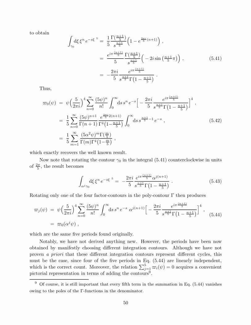
to obtain ∫

γ0

dξ ξn e−sξ5

=1

5

Γ(n+15 )

sn+1

5

(1 − e

2πi5 (n+1)

),

=eiπ

(n+1)5

5

Γ(n+15 )

sn+15

(− 2i sin

(n+1

5 π))

,

= −2πi

5

eiπ(n+1)

5

sn+15 Γ

(1 − n+1

5

) .

(5.41)

Thus,

0(ψ) = ψ( 5

2πi

)4∞∑

n=0

(5ψ)n

n!

∫ ∞

0

ds sn e−s[− 2πi

5

eiπ(n+1)

5

sn+15 Γ

(1 − n+1

5

)]4,

=1

5

∞∑

n=0

(5ψ)n+1

Γ(n+ 1)

e2πi5 2(n+1)

Γ4(1−n+1

5

)∫ ∞

0

ds sn+15 −1 e−s ,

=1

5

∞∑

m=1

(5α2ψ)mΓ(m5 )

Γ(m)Γ4(1−m

5

) ,

(5.42)

which exactly recovers the well known result.

Now note that rotating the contour γ0 in the integral (5.41) counterclockwise in units

of 2π5

, the result becomes

∫

αjγ0

dξ ξn e−sξ5

= −2πi

5

eiπ(n+1)

5 αj(n+1)

sn+15 Γ

(1 − n+1

5

) . (5.43)

Rotating only one of the four factor-contours in the poly-contour Γ then produces

j(ψ) = ψ( 5

2πi

)4 ∞∑

n=0

(5ψ)n

n!

∫ ∞

0

ds sn e−s αj(n+1)[− 2πi

5

eiπ(n+1)

5

sn+15 Γ

(1 − n+1

5

)]4,

= 0(αjψ) ,

(5.44)

which are the same five periods found originally.

Notably, we have not derived anything new. However, the periods have been now

obtained by manifestly choosing different integration contours. Although we have not

proven a priori that these different integration contours represent different cycles, this

must be the case, since four of the five periods in Eq. (5.44) are linearly independent,

which is the correct count. Moreover, the relation∑5

j=1i(ψ) = 0 acquires a convenient

pictorial representation in terms of adding the contours9.

9 Of course, it is still important that every fifth term in the summation in Eq. (5.44) vanishes

owing to the poles of the Γ-functions in the denominator.

50

6. Concluding Remarks

We have described a method for computing the periods of Calabi-Yau models which is

applicable to the majority of currently known Calabi–Yau manifolds and Landau-Ginzburg

models. We recall that the calculation of the periods provides the basis for the explicit

computation of the physically interesting quantities such as the physically normalized

Yukawa couplings of the effective low energy theory and the threshold corrections to the

gauge coupling constants [44] for (2, 2) models. Knowledge of the periods permits also the

computation of the numbers of instantons of the corresponding Calabi–Yau manifold [3–7].

For a recent advance concerning instantons of genus one, see Ref. [45].

Therefore, the present work brings us significantly closer to having a complete control

of the low energy effective action for any (2, 2) vacuum. It is illustrative to compare this

with the conformal field theory (CFT) techniques used in the case of free theories and coset

spaces. Even though the CFT is well known in those cases, the calculation of the effective

couplings is always restricted to particular points (Gepner–Kazama–Suzuki models) or a

subregion (orbifolds) of the whole moduli space of the given (2, 2) model. Remarkably,

the geometrical approach used here has now achieved the same level of calculability as

in the exact CFT’s cases, even though the underlying CFT’s are known explicitly only

for special subregions or particular points of the moduli space. These achievements are

due to the methods developed during the last few years using topological and algebro-

geometrical techniques as well as special geometry and mirror symmetry. In addition,

this method has the advantage that the dependence of the couplings on the whole moduli

space is considered, whence the structure of the full modular group can be obtained. An

illustrative example to compare both approaches is the mirror of the Z3 orbifold [46]. In

this case, the geometrical and the CFT methods give identical results for the relevant

quantities. However, the explicit dependence of the couplings on the twisted moduli of

the corresponding orbifold model may now be obtained using geometrical techniques—

which goes beyond the common CFT practice. It would be interesting to obtain a similar

level of computability for all couplings (including the E6 1’s) and eventually extend these

techniques to (0, 2) models, where the geometrical techniques are far less well developed.

In principle the procedure presented here may be extended to other cases that were

not considered, such as complete intersection spaces in products of weighted projective

spaces [47] or more general Landau-Ginzburg models that do not have a standard Calabi-

Yau interpretation [46]. Also, the methods of Sections 2 and 3 cover only the dependence of

the Kahler class periods of CICY manifolds on the parameters corresponding to the Kahler

classes of the embedding space or the mirror model. This appears to be suitably generalised

by the inclusion of non-polynomial deformations and the alternate expansion method of

Section 4. Another example of this type concerns the mirror of the Z3 orbifold [46].

51

Finally, even though we can write the fundamental period for very large classes of

models, the explicit determination of the full set of periods and the identification of the

integral symplectic basis requires an understanding of the singularity structure of each

moduli space and, at present, this has to be done model by model. Similar remarks apply

also to the determination of the modular group since this is also largely determined by the

singularity structure of the moduli space.

Acknowledgments: We are indebted to Paul Green and Sheldon Katz for discussions

and corrections. This work was supported by the American-Scandinavian Foundation, the

Fulbright Program, the NSF grants PHY 8904035 and PHY 9009850, the Robert A. Welch

foundation and the Swiss National Science Foundation. P.B., X.D. and F.Q. would like to

thank the Theory Division at CERN for hospitality and P.C. and X.D. wish to acknowledge

the hospitality of the Institute for Theoretical Physics in Santa Barbara, California, where

some of this work was done. A.F. thanks the Institut de Physique of the Universite de

Neuchatel and the ICTP, Trieste for hospitality while part of this research was done as

well as the Centro Cientıfico IBM-Venezuela for the use of its facilities.

52

References

1. A. Strominger, Commun. Math. Phys. 133 (1990) 163.

2. P. Candelas and X. C. de la Ossa, Nucl. Phys. B355 (1991) 455.

3. P. Candelas, X. de la Ossa, P. Green and L. Parkes, Nucl. Phys. B359 (1991) 21.

4. D. Morrison, “Picard-Fuchs Equations and Mirror Maps for Hypersurfaces”, in

Essays on Mirror Symmetry, ed. S.-T. Yau (Intl. Press, Hong Kong, 1992).

5. A. Font, Nucl. Phys. B391 (1993) 358.

6. A. Klemm and S. Theisen, Nucl. Phys. B389 (1993) 153.

7. P. Candelas, X. de la Ossa, A. Font, S. Katz and D. Morrison, in preparation.

8. M. Kreuzer and H. Skarke, Nucl. Phys. B388 (1992) 113.

9. M. Kreuzer and H. Skarke, Commun. Math. Phys. 150 (1992) 137.

10. A. Klemm and R. Schimmrigk, “Landau-Ginzburg Vacua”, CERN preprint CERN-

TH-6459/92, Universitat Heidelberg report HD-THEP-92-13.

11. P. Berglund and T. Hubsch, Nucl. Phys. B393 (1993) 377, also in Essays on Mirror

Manifolds, p.388, ed. S.-T. Yau, (Intl. Press, Hong Kong, 1992).

12. B.R. Greene and M.R. Plesser: “Mirror Manifolds, A Brief Review and Progress

Report”, Cornell and Yale University preprints CLNS 91-1109, YCTP-P32-91.

13. T. Hubsch, Commun. Math. Phys. 108 (1987) 291.

14. P. Green and T. Hubsch, Commun. Math. Phys. 109 (1987) 99.

15. P. Candelas, A.M. Dale, C. A. Lutken and R. Schimmrigk,

Nucl. Phys. B298 (1988) 493.

16. T. Hubsch: Calabi–Yau Manifolds—A Bestiary for Physicists

(World Scientific, Singapore, 1992).

17. S.-T. Yau: in Proc. of Symposium on Anomalies, Geometry, Topology , pp.395,

esp. the Appendix, by G. Tian and S.-T. Yau, pp.402-405, eds. W.A. Bardeen and

A.R. White (World Scientific, Singapore, 1985).

18. B.R. Greene, C. Vafa and N.P. Warner, Nucl. Phys. B324 (1989) 371.

19. T. Hubsch, Class. Quantum Grav. 8 (1991) L31.

20. P. Berglund, B.R. Greene and T. Hubsch, Mod. Phys. Lett. A7 (1992) 1885.

21. A. Libgober and J. Teitelbaum, “Lines on Calabi–Yau Complete Intersections, Mir-

ror Symmetry and Picard Fuchs Equations”, University of Illinois Report (1992).

22. V. Batyrev, Duke Math. J. 69 (1993) 349.

23. R. Schimmrigk: Phys. Lett. 193B (1987) 175.

24. V. Batyrev and D. Van Straten, “Generalized Hypergeometric Functions and Ratio-

nal Curves on Calabi–Yau Complete Intersections in Toric Varieties”, Universitat

Essen report in preparation.

25. T. Hubsch and S.-T. Yau, Mod. Phys. Lett. A7 (1992) 3277.

53

26. P. Green and T. Hubsch, Commun. Math. Phys. 113 (1987) 505.

27. P. Berglund and T. Hubsch, “Couplings for Compactification”, Howard University

preprint HUPAPP-93/2, Nucl. Phys. B (in press).

28. M. Lynker and R. Schimmrigk, Phys. Lett. 249B(1990) 237.

29. B.R. Greene and R. Plesser, in Essays on Mirror Symmetry, p.1, ed. S.-T. Yau

(Intl. Press, Hong Kong, 1992).

30. M. Atiyah, R. Bott and L. Garding, Acta Math. 131 (1973) 145.

31. P. Candelas, Nucl. Phys. B298 (1988) 458.

32. A. Erdelyi, F. Oberhettinger, W. Magnus and F. G. Tricomi, Higher Transcendental

Functions, 3 Vols., (McGraw–Hill, New York, 1953).

33. P. Berglund and S. Katz, in preparation.

34. Y.L. Luke, The Special Functions and Their Approximations, 2 Vols.,

(Academic Press, New York, 1969).

35. A. Klemm and Theisen: “ Mirror Maps and Instanton Sums for Complete Intersec-

tions in Weighted Projective Space”, Munich University preprint LMU-TPW-93-08.

36. S. Katz, private communication.

37. A. C. Cadavid and S. Ferrara, Phys. Lett. 267B (1991) 193.

38. B. Blok and A. Varchenko, Int. J. Mod. Phys. A7, (1992) 1467.

39. W. Lerche, D. J. Smit and N. P. Warner, Nucl. Phys. B372 (1992) 87.

40. A. Ceresole, R. D’Auria, S. Ferrara, W. Lerche and J. Louis, Int. J. Mod. Phys.A8

(1993) 79.

41. P. Griffiths, Ann. Math. 90 (1969) 460.

42. P. Candelas, X. C. de la Ossa and S. Katz, work in progress

43. R. Schimmrigk: “Critical Superstring Vacua from Noncritical Manifolds: A Novel

Framework”, Universitat Heidelberg report HD-THEP-92-29.

44. L. Dixon, Talk Presented at the Mirror Symmetry Workshop, MSRI (1991),

unpublished.

45. M. Bershadsky, S. Cecotti, H. Ooguri and C. Vafa, “Holomorphic Anomalies in

Topological Field Theories”, Harvard University preprint HUTP-93/A008.

46. P. Candelas, E. Derrick and L. Parkes, “Generalized Calabi-Yau Manifolds and the

Mirror of a Rigid Manifold”, CERN preprint CERN-TH.6831/93 (1993).

47. B. Greene, S.-S. Roan and S.-T. Yau, Commun. Math. Phys. 142 (1991) 245.

54