arX

iv:h

ep-t

h/04

0921

5v2

8 O

ct 2

004

DAMTP-2004-85

hep-th/0409215

On the Explicit Construction and

Statistics of Calabi-Yau Flux Vacua

Joseph P. Conlon 1 and Fernando Quevedo 2

DAMTP, Centre for Mathematical Sciences,

Wilberforce Road, Cambridge, CB3 0WA, UK

Abstract

We explicitly construct and study the statistics of flux vacua for type IIB

string theory on an orientifold of the Calabi-Yau hypersurface P4[1,1,2,2,6],

parametrised by two relevant complex structure moduli. We solve for

these moduli and the dilaton field in terms of the set of integers defin-

ing the 3-form fluxes and examine the distribution of vacua. We compare

our numerical results with the predictions of the Ashok-Douglas density

det(−R−ω), finding good overall agreement in different regions of moduli

space. The number of vacua are found to scale with the distance in flux

space. Vacua cluster in the region close to the conifold singularity. Large

supersymmetry breaking is more generic but supersymmetric and hierar-

chical supersymmetry breaking vacua can also be obtained. In particular,

the small superpotentials and large dilaton VEVs needed to obtain de Sit-

ter space in a controllable approximation are possible but not generic. We

argue that in a general flux compactification, the rank of the gauge group

coming from D3 branes could be statistically preferred to be very small.

1e-mail: J.P.Conlon@damtp.cam.ac.uk2e-mail: F.Quevedo@damtp.cam.ac.uk

Contents

1 Introduction 2

2 General Framework 4

2.1 The Model . . . . . . . . . . . . . . . . . . . . . . . . . . . . . . . 42.2 Fluxes, Periods and Moduli . . . . . . . . . . . . . . . . . . . . . 6

3 Vacua Statistics 11

3.1 The Vicinity of ψ = φ = 0 . . . . . . . . . . . . . . . . . . . . . . 113.2 The Vicinity of the Conifold Locus . . . . . . . . . . . . . . . . . 14

4 Summary and Discussion 18

1 Introduction

It has been claimed that the current status of string theory resembles that of par-ticle physics in the early 1960’s[1] in the sense that there are many experimentalresults but no organising principle. For string theory the place of the experimentsis taken by the many explicit string vacua that have been constructed over theyears. One desirable avenue towards understanding string theory involves thedevelopment and questioning of its basic principles. Another less ambitious butequally important program is to explore the large variety of string vacua withthe hope of learning more about the structure of the theory and of finding someof its phenomenological and/or cosmological implications.

In the phenomenological direction there has been substantial progress throughthe construction of string vacua with properties very similar to the standardmodel[2]. In cosmological applications, concrete ways have been found to realiseinflation within string theory [3]. Furthermore the construction and study ofstring vacua and their properties has played an important role over the yearsin the understanding of the theory itself, as exemplified by the discovery of T -duality [4], mirror symmetry [5] and S-duality [6]. Mirror symmetry providesprobably the most direct example in the sense that even though there were sev-eral ideas about its existence, the actual realisation came only after a plot ofmany of the vacua was found to be essentially symmetric under the exchange ofcomplex and Kahler structure moduli, thus providing ‘experimental’ evidence forthis symmetry.

Whether we like it or not, the lack of a close experimental test of the theoryand the large abundance of vacua suggest that a reasonable direction to pur-sue is to create a large database of string vacua as a temporary substitute forexperimental results. This database may eventually be used to extract model-

2

independent features of string vacua that may be testable. It may also give ussome further hints into the structure of the theory itself.

These issues have been recently clarified through the study of antisymmetrictensor flux compactifications [7, 8]. In the absence of these fluxes there weremyriads of vacua, each with a large continuous degeneracy parametrised by themoduli of the compactification space. Turning on the fluxes substantially reducesthis degeneracy by making it discrete, owing to the Dirac quantisation conditionfor the fluxes. The fluxes can fix the values of the moduli, which then belong toa discrete set determined by the allowed fluxes. This huge discrete degeneracymakes a statistical analysis suitable for the study of vacua. The stabilisationof the dilaton and complex structure moduli is relatively straightforward, butflux compactifications may also enable the construction of metastable vacua withpositive cosmological constant with the Kahler structure moduli also stabilisedas in the KKLT scenario [9, 10].

Even though the number of flux vacua appears to be enormous for a generalCalabi-Yau manifold, there are a number of requirements that must be satisfiedfor these vacua to be acceptable. First, as the entire framework is founded on aweak coupling approximation, only solutions leading to values of Im τ ≫ 1, whereτ = C0 + ie−φ is the dilaton-axion field that measures the string coupling. Theself-duality of type IIB under the SL(2,Z) S-duality symmetry implies that anysolution can be mapped to the fundamental domain. Having mapped solutionsto this region we can then only trust values of the dilaton substantially greaterthan one. As we will discuss in section 2.2, this is expected to be naturallysuppressed statistically, with the proportion of vacua with Im τ > τ0 falling as

1Im τ0

. Secondly, the fluxes may or may not break supersymmetry by themselvesand it is of interest to know the value of the supersymmetry breaking scale foreach model. This is more urgent if the models are embedded in the full KKLTscenario in which non-perturbative superpotentials are also included to fix theKahler moduli3. In order to guarantee a volume sufficiently larger than the stringscale and believe the four-dimensional effective field theory analysis, the value ofthe gravitino mass induced only by the fluxes has to be hierarchically small, acondition that is not straightforward to satisfy.

Recently, Douglas and collaborators have developed statistical techniques tostudy string vacua e.g.[15, 16, 17]. In particular, in [16], a general formula wasproposed that captures the statistical nature of the vacua, in terms of a densitygiven by det(−R−ω) where R is the curvature two form and ω the Kahler two-form on moduli space. In [18] the validity of this formula was successfully testedin a one-modulus example.

3In the KKLT scenario, the combination of fluxes that themselves break supersymmetry

with a non-perturbative superpotential results in a supersymmetric minimum. In this case

supersymmetry is broken only after the introduction of anti D3-branes [9, 11], magnetic fluxes

on D7 branes [12], by α′ corrections [13], or in other vacua of the complex structure moduli[14].

3

In this note we extend this analysis to a simple two-modulus compactifica-tion, corresponding to the three-fold realisable as a hypersurface in the weightedprojective space P[1,1,2,2,6]. We turn on 3-form fluxes and use the techniques ofCandelas et al [19, 20, 21] to compute the periods. This allows us to determinethe superpotential for the dilaton and complex structure moduli fields. We usea Monte Carlo analysis to study the distribution of vacua in the vicinities of theLandau-Ginzburg and conifold regions of moduli space. We compute the Ashok-Douglas index and compare with our results, finding good general agreement.We also investigate the distribution of values of the dilaton field as well as thesupersymmetry breaking scale.

While in the last stages of this project we received an article [22] that dis-cusses the Ashok-Douglas density for the same Calabi-Yau without performingthe numerical analysis.

2 General Framework

We here review the construction of the particular Calabi-Yau we study, and thecalculation of its periods[20, 21]. Some explicit flux compactifications on thisCalabi-Yau are also presented in [23].

2.1 The Model

There exist many Calabi-Yau manifolds that can be realised as hypersurfaces inweighted projective space. The weighted projective space P

4[k0,k1,k2,k3,k4]

is definedby

(w0, w1, w2, w3, w4) ≡ (λk0w0, λk1w1, λ

k2w2, λk3w3, λ

k4w4)

and has four complex dimensions. To obtain a space of three complex dimensionswe restrict to the hypersurface P (wi) = 0, where P is a polynomial in the wi.The condition that such a hypersurface be Calabi-Yau is that deg(P ) =

∑4i=0 ki.

In this paper we will make use of the Calabi-Yau hypersurface in P4[1,1,2,2,6], which

arises fromw12

0 + w121 + w6

2 + w63 + w2

4 = 0. (1)

We shall denote this manifold by M. M has h1,1 = 2 and h2,1 = 128. Thenumber of complex structure moduli is determined by the number of monomialdeformations of degree 12 that can be added to (1). There are two complexstructure moduli that are particularly important, which we shall denote by ψ

and φ. These perturb (1) to

P (wi) = w120 +w12

1 +w62 +w6

3 +w24 − 12ψ (w0w1w2w3w4)− 2φ

(

w60w

61

)

= 0. (2)

Their significance is due to their survival in the mirror manifold W, obtained byidentifying points in M related by the action of G, the maximal group of scaling

4

symmetries of (1). G here is Z2 × Z26, and its action is represented by

Z2 : (w1, w4) → (αw1, αw4) with α2 = 1,

Z6 : (w1, w3) → (β5w1, βw3) with β6 = 1,

Z′6 : (w1, w2) → (γ5w1, γw2) with γ6 = 1.

These manifestly leave equation (2) invariant. All other degree 12 deformationsof equation (2) are not well defined on the mirror. As W has h1,1 = 128 andh2,1 = 2, it is an example of a Calabi-Yau with two complex structure moduli.Both M and W develop a conifold singularity when 864ψ6+φ = 1. This conditionfollows from requiring P (wi) = ∇P (wi) = 0 with ∇∇P non-singular.

The Ashok-Douglas index density describes the statistics of the class of mod-els described in [8], namely flux compactifications of type IIB orientifolds. Tofit the above model into this framework, we embed it into an F -theory modelwith an orientifold limit according to Sen’s prescription[24]. The correspond-ing elliptically fibered four-fold is the hypersurface in weighted projective spaceP

5[1,1,2,2,12,18] with χ = 19728. The associated tadpole cancellation condition then

reads[25]:

ND3 +Nflux =χ

24= 822 ≡ L. (3)

Here ND3 is the net number of D3 branes and Nflux the contribution of the fluxesto the D3 brane charge,

Nflux =1

(2π)4 α′2

∫

M

H3 ∧ F3. (4)

Here H3 = dB2 and F3 = dC2 are the NS-NS and R-R 3-forms respectively.To cancel tadpoles in a supersymmetric fashion we then require the fluxes tocarry at most 822 units of D3-brane charge (this number as usual measures theamount of negative D3 brane charge coming from D7 branes and orientifolds, inthe orientifold realisation of the model).

In the low-energy approximation, the moduli of the Calabi-Yau appear asscalar fields in a supergravity theory. The effective four-dimensional N = 1supersymmetric field theory is determined by the Kahler potential KT (ξp, φi)and the superpotential W (φi), where ξp (p = 1, . . . , h1,1) represent the Kahlermoduli and φi (i = 1, . . . h2,1 + 1) the dilaton and complex structure moduli. Thetree-level Kahler potential takes the form

KT (ξp, φi) = K(ξp) +K(φi), (5)

where K is the Kahler potential for the Kahler moduli and K that for the dilatonand complex structure moduli. We will write an explicit expression for K in thenext section. As for K, the only information we need to provide is that it is of

5

the no-scale form, in the sense that K−1 qp K

pKq = 3 where p and q label theKahler moduli.

The appropriate superpotential for non-vanishing fluxes was proposed byGukov, Vafa and Witten [25] and takes the form

W =

∫

M

(F3 − τH3) ∧ Ω. (6)

τ is the complex dilaton-axion field and Ω the holomorphic (3, 0) form for theCalabi-Yau M.

The combination of the fact that W does not depend on the Kahler moduliand the no-scale structure of the Kahler potential implies that the effective scalarpotential is simply given by

V = eKT

(

DiWDjWK−1ij

)

, (7)

where DiW = ∂iW + (∂iK)W (in Planck mass units). Therefore, to stabilisethese fields at the minimum of the potential we need DiW = 0. The Kahlermoduli only appear in the potential in the eKT overall factor and are not fixed.We will omit these fields in the rest of this paper except for pointing out that theno-scale structure implies that the order parameter for supersymmetry breakingis

DpW = (∂pK)W. (8)

Thus a non-vanishing value of the superpotential W implies supersymmetrybreaking by the F -term of the Kahler structure moduli. Since a Kahler transfor-mation K → K + f + f , W → e−fW leaves the action invariant, the value of Wcan always be rescaled and a more appropriate, Kahler transformation invariant,measure of supersymmetry breaking is the gravitino mass, given by

m23/2 = eK |W |2. (9)

Notice that in the KKLT construction, a non-perturbative superpotential de-pending on these fields is added [9, 11], breaking the no-scale structure and fixingthe Kahler moduli. Anti D3-branes (or magnetic fluxes on the D7-branes [12])are introduced in order to lift the minimum of the potential to a positive value.This can certainly be done in the present model, but as we have nothing new tosay in this respect we concentrate on the dependence of the theory on the dilatonand complex structure moduli, to which we now turn.

2.2 Fluxes, Periods and Moduli

For any Calabi-Yau 3-fold, the middle homology and cohomology are naturallyexpressed in terms of a symplectic basis. That is, there exists a basis of 3-cycles

6

Aa and Bb and a basis of 3-forms αa and βb (where a, b = 1, 2 . . . (h2,1 + 1)), suchthat in homology

Aa ∩Bb = −Bb ∩Aa = δab ,

Aa ∩ Ab = Ba ∩ Bb = 0, (10)

and∫

Ab

αa = −

∫

Ba

βb = δba, (11)

∫

M

αa ∧ βb = −

∫

M

βb ∧ αa = δba. (12)

Such a symplectic basis is only defined up to Sp(2n,Z) transformations, as thesepreserve the symplectic intersection form. The periods are defined as the integralof the holomorphic 3-form Ω over these cycles,

∫

Aa

Ω = za,

∫

Bb

Ω = Ga. (13)

The periods are encapsulated in the period vector, Π = (G1, . . . ,Gn, z1, . . . , zn),where n = h2,1 + 1. This inherits the holomorphic freedom of Ω and is definedup to holomorphic rescalings Ω → f(φi)Ω. Note that Π = Π(φi), where φi arethe complex structure moduli of the Calabi-Yau.

Given the vector of periods Π(φi), the Kahler potential on complex structuremoduli space is given by [26]

K(τ, φi) = − ln(−i(τ − τ )) − ln

(

i

∫

Ω ∧ Ω

)

= − ln(−i(τ − τ )) − ln(−iΠ† · Σ · Π) (14)

≡ Kτ +Kφ.

where

Σ =

(

0 1n−1n 0

)

and τ is the dilaton-axion. We can then compute the metric on moduli space,

gαβ = ∂α∂βK, (15)

and the Riemann and Ricci curvatures

Rλµνρ = −∂ν(g

λα∂µgρα),

Rµν = Rλµνλ = −∂µ∂ν log(det g). (16)

7

In terms of the periods, the Gukov-Vafa-Witten superpotential is

W = (2π)2α′(f − τh) · Π(φi), (17)

where f = (f1, . . . , f6) and h = (h1, . . . , h6) are integral vectors of fluxes alongthe cycles. The fluxes F3 and H3 are elements of H3(M,Z) and satisfy the fluxquantisation conditions

1

(2π)2α′

∫

Σ3

F ∈ Z,1

(2π)2α′

∫

Σ3

H ∈ Z, (18)

where Σ3 is an arbitrary 3-cycle. The amount of D3-brane charge carried by thefluxes is then

Nflux = fT · Σ · h. (19)

The stabilisation of the complex structure moduli φi is governed by the fol-lowing equations

DφiW = ∂φi

W + (∂φiK)W = 0,

DτW = ∂τW + (∂τK)W = 0. (20)

Distinct choices of fluxes stabilise the complex structure moduli at discrete pointsin moduli space. As the total number of flux vacua is very large, the distributionof discrete flux vacua can be approximated by a continuous distribution. Treatingthe fluxes as non-quantised, Ashok and Douglas[16] derived a formula for an indexthat gives an estimate of the total number of vacua with Nflux < L on a regionX of moduli space

Ivac(Nflux ≤ L) =(2πL)K(−1)

K2

πn+1K!

∫

X

det(−R− 1 · ω) (21)

where ω is the Kahler form and R the curvature two-form on moduli space. Informula (21) K is the number of cycles along which flux is wrapped and L thetotal available D3-brane charge. In a comparison with numbers of explicit vacua,the constant prefactor is obviously not relevant.

We will now restrict to cases where the Calabi-Yau M has two complex struc-ture moduli. The region X includes the dilaton-axion moduli space. The weightedvacuum density over the Calabi-Yau moduli space is then evaluated to be[28]

dµ = gτ τdτ ∧ dτ ∧(

4π2c2 − det(gaa)dψ1 ∧ dψ1 ∧ dψ2 ∧ dψ2

)

, (22)

where gτ τ = − 1(τ−τ )2

and c2, the second Chern class of M, is given by

c2 =1

8π2(tr(R∧R) − trR∧ trR) . (23)

8

(22) may be rewritten as

dµ = gτ τdτ ∧dτ ∧dψ1 ∧dψ1 ∧dψ2 ∧dψ2

[

ǫabǫab(

R1aa1R

2bb2 −R1

aa2R2bb1

)

− det gaa

]

.

(24)To evaluate both (20) and (22) we must obtain a knowledge the periods, which

in general is a highly non-trivial task. However, the manifold defined by (2) isof a class that has been extensively studied. The relevant periods have beencomputed in [20, 21], following the classic treatment of the quintic[19], and wewill borrow their results. For the Calabi-Yau described by the hypersurface

P =

4∑

j=0

xd/kj

j − dψx0x1x2x3x4 −d

q0φx

q00 x

q11 x

q22 x

q33 x

q44 = 0, (25)

the fundamental period in the large ψ region is given by

f(ψ, φ) =∞

∑

l=0

(q0l!)(dψ)−q0l(−1)l

l!Π4i=1(

ki

d(q0 − qi)l)!

ul(φ), (26)

where

ul(φ) = (Dφ)l[ lD

]∑

n=0

l!Π4i=1(

ki

d(q0 − qi)l)!(−Dφ)−Dn

(l −Dn)!n!Π4i=1(

kiqiq0n+ ki

d(q0 − qi)l)!

. (27)

This is obtained by direct integration of Ω and satisfies the Picard-Fuchs equation.There are other independent solutions to the Picard-Fuchs equation having alogarithimic dependence on ψ. In total there are six independent solutions, onefor each 3-cycle, and the actual periods are a linear combination of these.

The two regions of moduli space that will most interest us are the vicinities ofthe Landau-Ginzburg point ψ = φ = 0 and the the conifold locus 864ψ6 +φ = 1.To obtain a basis of periods in the small ψ region, we analytically continue (26)to obtain

f (ψ, φ) = −2

d

∞∑

n=1

Γ(

2nd

)

(−dψ)n u− 2nd

(φ)

Γ (n) Γ(

1 − nd

(k1 − 1))

Γ(

1 − k2nd

)

Γ(

1 − k3nd

)

Γ(

1 − k4nd

) .

(28)Here uν(φ) is related to the hypergeometric functions and is defined through thecontour integral

uν(φ) =2ν

π

∫ 1

−1

dζ√

1 − ζ2(φ− ζ)ν. (29)

The contour integral is initially defined for Im(φ) > 0 and then defined over therest of the plane by deforming the integral contour. The branch cuts, which areunavoidable when ν is non-integral, start at ±1 and run to ±∞.

9

We may derive a basis of periods from the fundamental period in a simplemanner. If we define

j(ψ, φ) =−(2πi)3

ψf(α

jψ, αjq0φ) (30)

then (ψ, φ) = (0(ψ, φ), 1(ψ, φ), 2(ψ, φ), 3(ψ, φ), 4(ψ, φ), 5(ψ, φ)) givesa basis of periods known as the Picard-Fuchs basis. Naively (30) would seem togive 12 independent periods, but there are interrelations discussed in [20]. Thenet result is that, as expected, there are six independent periods. This basis ishowever not symplectic. A symplectic basis is given by

Π(ψ, φ) = m ·(ψ, φ). (31)

Here m is computed in [27, 23] and is given by

m =

−1 1 0 0 0 032

32

12

12

−12

−12

1 0 1 0 0 01 0 0 0 0 0−1

20 1

212

0 012

12

−12

12

−12

12

.

In principle, equation (31) completely determines the periods near ψ = 0.However, it involves the integral expression (29) for uν(φ) which is inconvenientfor a computational treatment. Such a treatment is facilitated by the power seriesexpansion of uν(φ) in the small φ region found in [20]. This is given by

uν (φ) =e

iπν2 Γ

(

1 + ν(k1−1)2

)

2Γ (−ν)

∞∑

m=0

eiπm/2Γ(

m−ν2

)

(2φ)m

m!Γ(

1 − m−νk12

) (32)

The region of convergence of equations (28), (29), and (32) is worth discussing.We will here be specific to the particular Calabi-Yau described in section 2. Thismanifold develops a conifold singularity when φ + 864ψ6 = ±1 and there is alsoa strong coupling singularity when φ = ±1. The regions of convergence aredetermined by the singularities. All three equations are only valid for |864ψ

6

φ±1| < 1

and equation (32) has the additional restriction |φ| < 1.We will also be interested in the periods near the conifold locus. As will

be further discussed in section (3.2), the periods here have a certain standardform. However, for their exact numerical determination, we will use the neolithicapproach, directly evaluating the power series (31) near the conifold locus.

Finally, the Calabi-Yau we work on is the original manifold M defined bythe locus of the polynomial (2), and not its mirror W. M has a total of 128complex structure moduli. We expect some to be removed by the orientifold

10

symmetry, but there will still be many which we are ignoring. The validity ofthis was explained in [23]. The group G is a symmetry of (2) and if we only turnon fluxes invariant under this symmetry then the superpotential can only havea higher-order dependence on the other moduli. It is thus consistent to set allother moduli equal to zero and focus only on the moduli in equation (2) and theirassociated fluxes. We will comment briefly on the general situation in the lastsection.

3 Vacua Statistics

The two natural regions for testing the Ashok-Douglas formula are the vicinitiesof the Landau-Ginzburg point ψ = φ = 0 and the conifold locus 864ψ6 + φ = 1.

3.1 The Vicinity of ψ = φ = 0

A symplectic basis for the periods was given in equation (31). Let us untanglethis in the vicinity of ψ = 0. We can expand Π(ψ, φ) as

Π = a(φ) + b(φ)ψ2 + c(φ)ψ4 + O(

ψ6)

. (33)

Here a, b and c are vector functions of φ whose explicit form arises from thecombination of equations (28), (32), (30) and (31). It can be checked that a† ·Σ ·b = a† · Σ · c = 0, implying

Π† · Σ · Π = (a† · Σ · a) + (b† · Σ · b)ψ2ψ2 + O(

|ψ|6)

,

and consequently

Kφ(ψ, φ) = − ln(

−iΠ† · Σ · Π)

= − ln(

−ia† · Σ · a)

− ln

(

1 +(b† · Σ · b)

(a† · Σ · a)ψ2ψ2 + O

(

|ψ|6)

)

= − ln(

−ia† · Σ · a)

−(b† · Σ · b)

(a† · Σ · a)ψ2ψ2 + O

(

|ψ|6)

. (34)

Equations (20) then have the form

1

ψDψW = 0 ⇒ (f − τh) ·

(

α1(φ) + α2(φ)ψ2 + α3(φ)ψ2)

= 0, (35)

DφW = 0 ⇒ (f − τh) ·(

β1(φ) + β

2(φ)ψ2

)

= 0, (36)

DτW = 0 ⇒ (f − τ h) · (a(φ) + b(φ)ψ2) = 0, (37)

where we have dropped terms of O (|ψ|4). Here α(φ) and β(φ) are complicatedfunctions of φ depending on the integral expressions for uν(φ). However, when

11

|φ| < 1 the use of the power series expansion in equation (32) coverts α(φ) andβ(φ) to a more tractable form. The leading behaviour of the metric gαβ = ∂α∂βK

is given by

gψψ ∼ ψψ, gψφ ∼ ψψ2φ, gφψ ∼ ψ2ψφ, gφφ ∼ 1.

This is consistent with our expectations - at the Landau-Ginzburg point ψ = φ =0 the metric becomes singular. The curvature 2-form R and the Chern class c2may be calculated straightforwardly from the full expressions for the metric usinga symbolic algebra program. Evaluating the Ashok-Douglas density, we find ithas leading behaviour

dµ ∼ gτ τ dτ ∧ dτ ∧ ψψdψ ∧ dψ ∧ dφ ∧ dφ.

The regions on which we compare the Ashok-Douglas formula to our empiricalresults are balls in ψ and φ space. We then expect as leading behaviour

N(vacua s.t. |ψ| < r1) ∼ r41,

N(vacua s.t. |φ| < r2) ∼ r22.

To test this expectation, we generated random fluxes and sought solutionsof equations (35) to (37) using a numerical root finder. The range of fluxesused was (-20, 20). This is not as large as one might prefer. However, a largerrange of fluxes resulted in solutions being produced insufficiently rapidly for ourpurposes. In order to be able to trust our truncation of the power series, we onlykept solutions satisfying

∣

∣

∣

∣

864ψ6

φ± 1

∣

∣

∣

∣

< 0.5 and |φ| < 0.75. (38)

When processing the numerical results, there is an important subtlety we mustaccount for4. It is well known that there is an exact SL(2,Z) symmetry of typeIIB,

τ →aτ + b

cτ + d,

(

F3

H3

)

→

(

a b

c d

) (

F3

H3

)

.

where a, b, c, d ∈ Z and ad−bc = 1. Thus each vacuum found has many physicallyequivalent SL(2,Z) copies that we should not double-count. One way to dealwith this would be to fix the gauge explicitly and then perform the Monte-Carloanalysis. Our approach is instead to weight each vacuum by the inverse of thenumber of copies it has within the sampled flux range. The purpose of this is toensure that vacua with many SL(2,Z) copies are not preferred.

As well as the SL(2,Z) symmetry, there is a monodromy near the Landau-Ginzburg point that needs similar treatment. From the definition of the periods

4We thank S. Kachru for bringing this to our attention.

12

(30), we can that they have a monodromy under (ψ, φ) → (αψ,−φ), whereα12 = 1, of

(ψ, φ) → a ·(ψ, φ),

where

a =

0 1 0 0 0 00 0 1 0 0 00 0 0 1 0 00 0 0 0 1 00 0 0 0 0 1−1 0 0 0 0 0

.

In the symplectic basis, the monodromy matrix A is given by m · a ·m−1. Theeffect of this monodromy is to produce a family of physically equivalent solutionsrelated by

(ψ, φ) → (α−1ψ,−φ),

f → f ·A,

h → h · A. (39)

When weighting vacua we need to find the total number of copies lying within thesampled flux range from all symmetries and monodromies. This has importantsystematic effects as vacua with smaller values of fi and hi, and thus smallervalues of Nflux, have more copies. A naive counting that neglects the symmetriesor monodromies that are present thus places undue emphasis on vacua withsmaller values of Nflux.

We looked at the distribution of vacua within fixed balls in ψ and φ space.In figure 1 we plot the number of vacua satisfying (38) and having |ψ| < r. Theresults are seen to agree well with the theoretical prediction. Likewise, figure 2shows the distribution of vacua for a ball |φ| < r in φ space. The continuousline again represents the cumulative number of vacua and the dots the rescalednumerical integration of

∫

|φ|<rdµ. The empirical results are again well captured

by the theoretical prediction. Finally, in figure 3 we examine the dependence ofthe number of vacua on the distance in flux space Nflux = fT ·Σ ·h. The graph isfit by N ∼ L4.3. This is surprising, as the expected scaling is L6. Furthermore, inthe vicinity of the Landau-Ginzburg point for an analogous one-modulus example,the correct L4 scaling is found[29]. As we will discuss further in section 4, webelieve our results are an artifact of the small flux range used, and that were alarger flux range used we would obtain the correct scaling. As we will shortlydescribe, in the vicinity of the conifold locus we do obtain the expected scalingwith a flux range of (−40, 40).

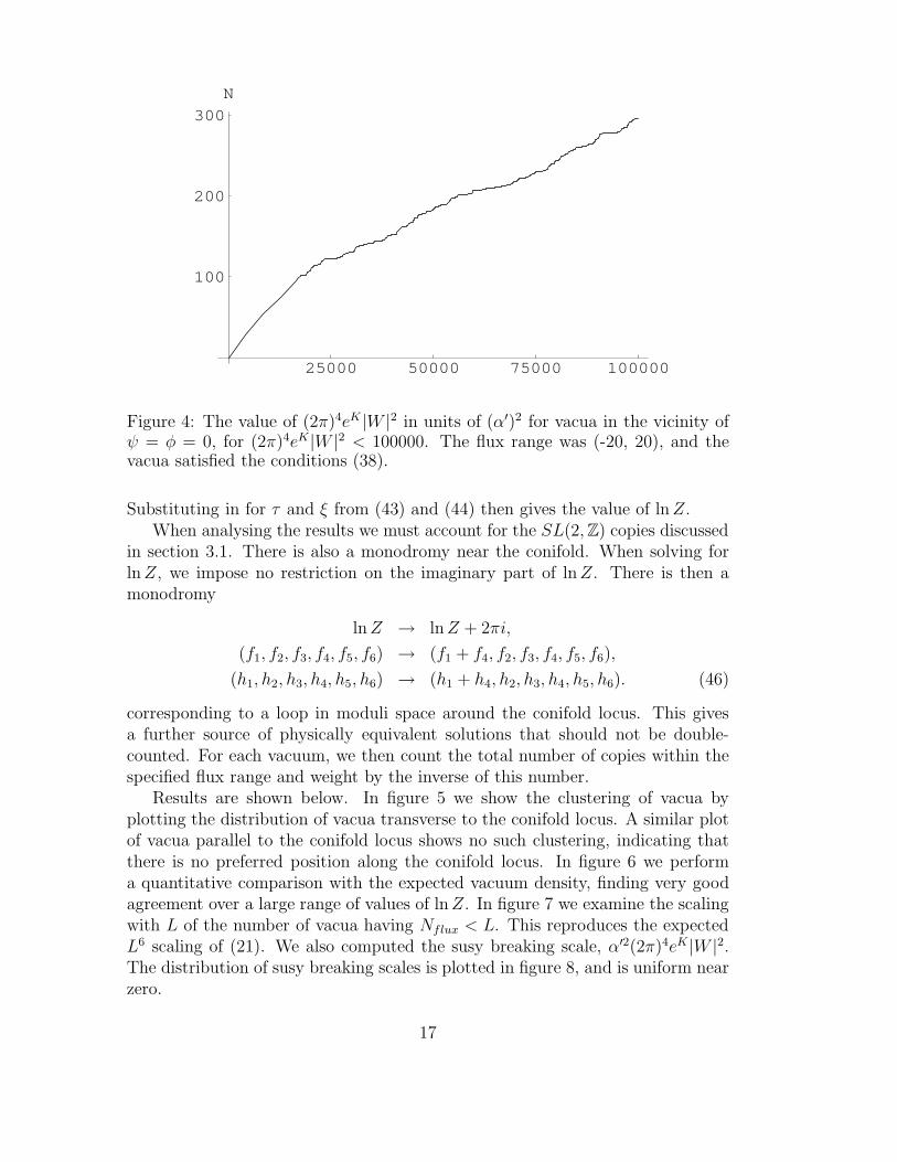
It is also of interest to study the supersymmetry breaking scale, as measuredby α′2(2π)4eK |W |2, for vacua in the vicinity of ψ = φ = 0. This is shown infigure 4. The most noticeable thing about this graph is that the distribution of

13

0.05 0.1 0.15 0.2 0.25r

200

400

600

800

1000

1200

N

Figure 1: Number of vacua with |ψ| < r. The value of N plotted includes aweighting due to the SL(2,Z) copies of each vacuum within the range of fluxessampled. The dots represent the numerical results, and the continuous line the(rescaled) numerical integration of

∫

|ψ|<rdµ, where dµ is the index density. The

flux range used was (-20,20).

the susy breaking scale is uniform near the origin and that the vast majority ofvacua therefore have a high supersymmetry breaking scale. We can also observefrom the structure of the graph that arbitrarily small values of the gravitinomass should exist as well as supersymmetric solutions. In reference [23], explicitsupersymmetric vacua were obtained for this model.

3.2 The Vicinity of the Conifold Locus

The Calabi-Yau M has a codimension one conifold degeneration along the modulispace locus 864ψ6 + φ = 1. The moduli space curvature diverges near a conifoldpoint and the expectation is that vacua should cluster near the conifold locus.

To study these vacua numerically, we must restrict attention to a small regionof the conifold locus where we can compute the periods explicitly. We takethis region to be the neighbourhood of the point φ = 0, ψ = ψ0 = 864−

1

6 . Ifwe write ψ = ψ0 + ξ and truncate the periods at first order in ξ and φ, thenΠ(ξ, φ) = (G1,G2,G3, z1, z2, z3) is approximated by

G1 = 3202ξ + 171.8φ+ O(ξ2, φ2, ξφ)

G2 = 4323 − i(1553ξ + 107.4φ) + O(ξ2, φ2, ξφ)

G3 = (−492.7 + 1976.8i) + (371.0 − 300.2i)ξ + (−259.0 − 59.0i)φ+ O(ξ2, φ2, ξφ)

z1 =−1

2πiG1 ln (G1) + 784.8i− 2306iξ − 44.35iφ+ O(ξ2, φ2, ξφ)

14

0.1 0.2 0.3 0.4 0.5 0.6 0.7r

200

400

600

800

1000

N

Figure 2: The weighted number of vacua, N , with |φ| < r. The dots represent thenumerical results and the continuous line the numerical integration of

∫

|φ|<rdµ,

rescaled by the same factor as in diagram 1.

z2 = (−994.6 − 184.8i) + (861.9 + 476.5i)ξ + (9.91 − 112.7i)φ+ O(ξ2, φ2, ξφ)

z3 = i(369.5 − 953.0ξ + 225.4φ) + O(ξ2, φ2, ξφ) (40)

The numerical values were found by evaluating the series (28) up to one hundredterms in ψ and twenty-five terms in φ. The values for the coefficients of theO(ξ, φ) terms were sensitive to the number of terms used in the power series atthe level of a couple of percentage points. We did not keep terms quadratic in ξand φ - inclusion of these would lead to O(ξ) corrections to the results below.

The general form of the periods is standard. The cycles corresponding toG2,G3, z2 and z3 are all remote from the conifold singularity, resulting in theassociated periods being both regular and non-vanishing near the conifold degen-eration. Recalling that the conifold is a cone with a base that is topologicallyS2 × S3, the cycle corresponding to G1 is the S3 that shrinks to zero size alongthe conifold locus. The period along this cycle is regular near the conifold locusand vanishing along it. Finally, the cycle corresponding to z1 is that dual tothe S3. It is therefore not uniquely defined and is in fact well known to have amonodromy under a loop around the conifold locus. Its period takes the form(

− 12πi

G1 ln(G1) + analytic terms)

.It is convenient to define Z =

(

3202171.8

)

ξ + φ and rewrite the periods as

G1 = 171.8Z,

G2 = 4323 + 107.4i Z − 3554i ξ,

G3 = 784.8 − (259 + 59i)Z + (5198 + 799i) ξ,

15

200 400 600 800L

50

100

150

200

250

300

350

N

Figure 3: The weighted number of vacua N with Nflux < L. 4.5 × 106 sets offlxues were generated, with values of L equally distributed between 0 and 800and the range of fluxes being (−20, 20). The results are fit by N ∼ L4.3.

z1 =−1

2πi171.8Z ln (Z) + 784.8 − 44.4i Z − 1479i ξ,

z2 = (−994.6 − 184.8i) + (9.91 − 112.7i)Z + (677 + 2577i) ξ,

z3 = i(369.5 + 225.4Z − 5154 ξ). (41)

Z is a measure of the distance from the conifold locus. We are interested invacua extremely close to the conifold locus - typically ln |Z| < −5 - and thuswe will regard |Z| << |ξ| << 1. Having set up the periods (41), we can nowcompute the Ashok-Douglas expectation for the index density and compare thiswith numerical results.

Let us now solve equations (20). First,

DτW = 0 ⇒ (f − τ h) · Π = 0 ⇒ τ =f · Π†

h · Π†. (42)

This can be written as

τ =a0 + a1ξ

b0 + b1ξ+ O(Z lnZ), (43)

where ai and bi are flux-dependent quantities. Next,

DξW = 0 ⇒ (f − τh) · (c0 + c1ξ + c2ξ + O(ξ2)) = 0. (44)

Using (43) this becomes a linear equation for ξ, easily solved to determine ξ andτ . We finally need the value of lnZ. This is obtained by considering

DZW = 0 ⇒ (f4 − τh4) lnZ = (d0 + d1τ) + (d2 + d3τ)ξ + (d4 + d5τ)ξ (45)

16

25000 50000 75000 100000

100

200

300

N

Figure 4: The value of (2π)4eK |W |2 in units of (α′)2 for vacua in the vicinity ofψ = φ = 0, for (2π)4eK |W |2 < 100000. The flux range was (-20, 20), and thevacua satisfied the conditions (38).

Substituting in for τ and ξ from (43) and (44) then gives the value of lnZ.When analysing the results we must account for the SL(2,Z) copies discussed

in section 3.1. There is also a monodromy near the conifold. When solving forlnZ, we impose no restriction on the imaginary part of lnZ. There is then amonodromy

lnZ → lnZ + 2πi,

(f1, f2, f3, f4, f5, f6) → (f1 + f4, f2, f3, f4, f5, f6),

(h1, h2, h3, h4, h5, h6) → (h1 + h4, h2, h3, h4, h5, h6). (46)

corresponding to a loop in moduli space around the conifold locus. This givesa further source of physically equivalent solutions that should not be double-counted. For each vacuum, we then count the total number of copies within thespecified flux range and weight by the inverse of this number.

Results are shown below. In figure 5 we show the clustering of vacua byplotting the distribution of vacua transverse to the conifold locus. A similar plotof vacua parallel to the conifold locus shows no such clustering, indicating thatthere is no preferred position along the conifold locus. In figure 6 we performa quantitative comparison with the expected vacuum density, finding very goodagreement over a large range of values of lnZ. In figure 7 we examine the scalingwith L of the number of vacua having Nflux < L. This reproduces the expectedL6 scaling of (21). We also computed the susy breaking scale, α′2(2π)4eK |W |2.The distribution of susy breaking scales is plotted in figure 8, and is uniform nearzero.

17

-1 -0.5 0.5 1

-1

-0.5

0.5

1

Figure 5: The value of Z for vacua near the conifold. We have restricted to|Z| < 0.0001 and have rescaled the above plot by 104. The flux range used was(-40,40).

4 Summary and Discussion

Let us briefly summarise our results.

1. We constructed a large class of flux vacua for the two-moduli Calabi-Yauthreefold P

4[1,1,2,2,6]. We independently computed the Ashok-Douglas density

and compared with our results. We find good agreement which improves asthe range of fluxes is increased. The number of vacua was limited mostlyby working in two patches in moduli space: the region near ψ = φ = 0 andthe region close to the conifold singularity φ+ 864ψ6 = ±1.

2. We found a large concentration of vacua close to the conifold singularityas predicted, with the detailed distribution of the vacua being in closeaccordance with expectation.

3. In both regions, the values of the superpotential are uniformly distributednear zero. As a consequence, large values of the superpotential, correspond-ing to a large supersymmetry breaking scale, are more abundant than smallones.

4. In both regions the number of models scaled as a power of the maximumpermitted value ofNflux, Lmax. In the vicinity of the conifold we reproducedthe expected L6 scaling. In the region close to the Landau-Ginzburg point

18

-140 -120 -100 -80 -60 -40 -20

400

800

1200

1600

N

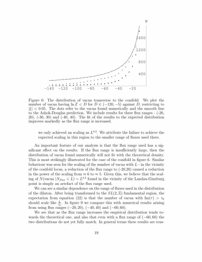
Figure 6: The distribution of vacua transverse to the conifold. We plot thenumber of vacua having lnZ < D for D ∈ (−120,−5) against D, restricting to|ξ| < 0.05. The dots refer to the vacua found numerically and the smooth lineto the Ashok-Douglas prediction. We include results for three flux ranges - (-20,20), (-30, 30) and (-40, 40). The fit of the results to the expected distributionimproves markedly as the flux range is increased.

we only achieved an scaling as L4.3. We attribute the failure to achieve theexpected scaling in this region to the smaller range of fluxes used there.

An important feature of our analysis is that the flux range used has a sig-nificant effect on the results. If the flux range is insufficiently large, then thedistribution of vacua found numerically will not fit with the theoretical density.This is most strikingly illustrated for the case of the conifold in figure 6. Similarbehaviour was seen for the scaling of the number of vacua with L - in the vicinityof the conifold locus, a reduction of the flux range to (-20,20) caused a reductionin the power of the scaling from ≈ 6 to ≈ 5. Given this, we believe that the scal-ing of N(vacua |Nflux < L) ∼ L4.3 found in the vicinity of the Landau-Ginzburgpoint is simply an artefact of the flux range used.

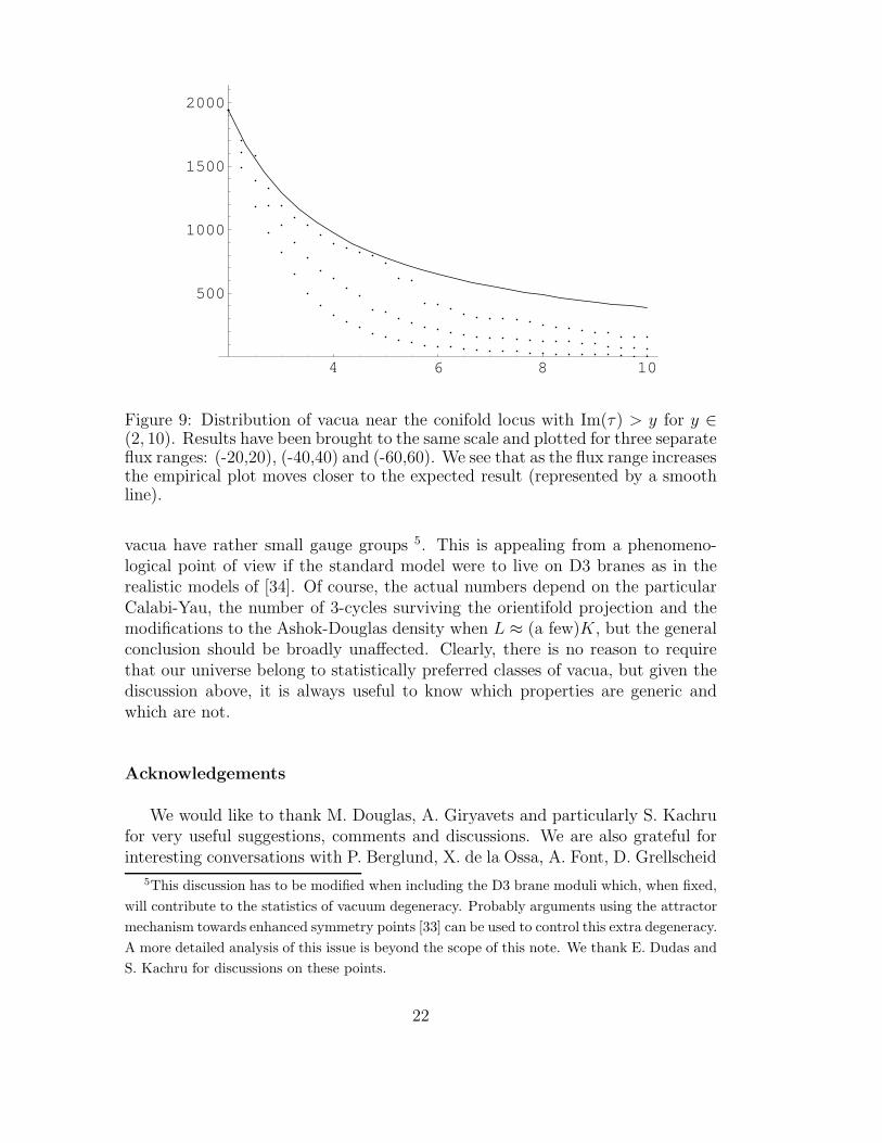
We can see a similar dependence on the range of fluxes used in the distributionof the dilaton. After being transformed to the SL(2,Z) fundamental region, theexpectation from equation (22) is that the number of vacua with Im(τ) > τ0should scale like 1

τ0. In figure 9 we compare this with numerical results arising

from using flux ranges (−20, 20), (−40, 40) and (−60, 60).We see that as the flux range increases the empirical distribution tends to-

wards the theoretical one, and also that even with a flux range of (−60, 60) thetwo distributions do not yet fully match. In general terms these results are reas-

19

200 400 600 800L

500

1000

1500

2000

2500

N

Figure 7: The weighted number of vacua with Nflux < L. The curve is fit well byN ∝ L6. The range of fluxes used was (-40,40).

suring in the sense that arbitrarily large values of the dilaton can be obtained,consistent with the weak coupling aproximation although they are not statisti-cally preferred.

As we have concentrated on only two complex structure moduli from a total of128, we have explored only a minuscule sample of the full set of flux vacua for thismodel. Still, we obtained sufficient statistics to see the expected distribution ofvacua. There is a clear computational obstruction to exploring the full spectrumof models for a given Calabi-Yau. However, we have seen that the consistencyrequirements of small string coupling and large volume are largely disfavouredstatistically. The relevant class of vacua will then be suppressed compared to thelarge estimated totals of order 10100. Nonetheless, given this large number it isreasonable to expect many solutions with very small values of the supersymmetrybreaking scale (which in the KKLT scenario becomes the large volume constraint).It would be desirable to develop techniques that, rather than simply countingthe number of vacua by numerically scanning the parameter space, select onlythose which satisfy the consistency and phenomenological requirements. Somesmall values of |W | can be found explicitly - [23] contains an example where|W | ≈ 4 × 10−3 and the first reference of [32] a case where |W |2 ≈ 2 × 10−4.The efficient discovery of phenomenologically acceptable vacua is harder; thetechniques recently developed in [30] may be of use in this regard. Finally, let usnote that in our study of this model we have addressed neither the issue of softsupersymmetry breaking terms induced solely by the fluxes nor α′ correctionsnor the non-perturbative superpotential required to complete the moduli fixing

20

25000 50000 75000 100000

250

500

750

1000

1250

1500

1750

Figure 8: The value of (2π)4eK |W |2 in units of (α′)2 for vacua near the conifold,for (2π)4eK |W |2 < 100000. The flux range was (-40, 40) and we restricted tovacua satisfying |ξ| < 0.05.

and lift the potential to get de Sitter space as in the KKLT scenario. For recentprogress in theses directions, [31, 13, 32] may be consulted.

Let us finish with a general observation. The Calabi-Yau considered here hash1,1 = 2 and h2,1 = 128. We have turned on fluxes along the cycles correspondingto only two of the 128 complex structure moduli. We would expect that someof the remaining moduli should be frozen out by the orientifold symmetry, butit would still be obviously impractical to attempt either to write down or tosolve the moduli stabilisation equations with all fluxes turned on. However, if weassume that the Ashok-Douglas density remains valid then we can say somethingabout the generic situation. Suppose we have K cycles supporting flux and that- as holds for this and many other F-theory models -

ND3 +Nflux = Lmax ∼ 1000. (47)

The Ashok-Douglas density (21) tells us that

N(vacua |Nflux < L∗) ∼ LK∗ . (48)

The fraction of vacua having ND3 ≥ n is then estimated by

N(vacua |Nflux ≤ Lmax − n)

N(vacua |Nflux ≤ Lmax)=

(Lmax − n)K

LKmax. (49)

For K ∼ 200, then for n = 5 this is approximately 1e≈ 0.36. We then see

that despite the large amount of D3-brane charge we have to play with, generic

21

4 6 8 10

500

1000

1500

2000

Figure 9: Distribution of vacua near the conifold locus with Im(τ) > y for y ∈(2, 10). Results have been brought to the same scale and plotted for three separateflux ranges: (-20,20), (-40,40) and (-60,60). We see that as the flux range increasesthe empirical plot moves closer to the expected result (represented by a smoothline).

vacua have rather small gauge groups 5. This is appealing from a phenomeno-logical point of view if the standard model were to live on D3 branes as in therealistic models of [34]. Of course, the actual numbers depend on the particularCalabi-Yau, the number of 3-cycles surviving the orientifold projection and themodifications to the Ashok-Douglas density when L ≈ (a few)K, but the generalconclusion should be broadly unaffected. Clearly, there is no reason to requirethat our universe belong to statistically preferred classes of vacua, but given thediscussion above, it is always useful to know which properties are generic andwhich are not.

Acknowledgements

We would like to thank M. Douglas, A. Giryavets and particularly S. Kachrufor very useful suggestions, comments and discussions. We are also grateful forinteresting conversations with P. Berglund, X. de la Ossa, A. Font, D. Grellscheid

5This discussion has to be modified when including the D3 brane moduli which, when fixed,

will contribute to the statistics of vacuum degeneracy. Probably arguments using the attractor

mechanism towards enhanced symmetry points [33] can be used to control this extra degeneracy.

A more detailed analysis of this issue is beyond the scope of this note. We thank E. Dudas and

S. Kachru for discussions on these points.

22

and K. Suruliz. FQ thanks the Aspen Center for Physics for hospitality duringits summer workshop ‘Strings and the Real World’, where part of this projectwas developed. JC thanks EPSRC for a research studentship. FQ is partiallysupported by PPARC and a Royal Society Wolfson award.

References

[1] J. Polchinski, What is string theory?, arXiv:hep-th/9411028; String duality:

A colloquium, Rev. Mod. Phys. 68 (1996) 1245 [arXiv:hep-th/9607050].

[2] For recent overall reviews see for instance: F. Quevedo, “PhenomenologicalAspects of D-branes” in *Trieste 2002, Superstrings and related matters*232-330; E. Kiritsis, “D-branes in standard model building, gravity and cos-mology,” Fortsch. Phys. 52 (2004) 200 [arXiv:hep-th/0310001].

[3] For recent reviews with many references see for instance: F. Quevedo,“Lectures on string / brane cosmology,” Class. Quant. Grav. 19

(2002) 5721 [arXiv:hep-th/0210292]; A. Linde, “Prospects of infla-tion,” arXiv:hep-th/0402051; C. P. Burgess, “Inflatable string theory?,”arXiv:hep-th/0408037.

[4] K. Kikkawa and M. Yamasaki, “Casimir Effects In Superstring Theories,”Phys. Lett. B 149 (1984) 357; N. Sakai and I. Senda, “Vacuum Energies OfString Compactified On Torus,” Prog. Theor. Phys. 75 (1986) 692 [Erratum-ibid. 77 (1987) 773].

[5] P. Candelas, M. Lynker and R. Schimmrigk, “Calabi-Yau Manifolds InWeighted P(4),” Nucl. Phys. B 341 (1990) 383; B. R. Greene andM. R. Plesser, “Duality In Calabi-Yau Moduli Space,” Nucl. Phys. B 338

(1990) 15.

[6] A. Font, L. E. Ibanez, D. Lust and F. Quevedo, “Strong - Weak CouplingDuality And Nonperturbative Effects In String Theory,” Phys. Lett. B 249

(1990) 35. C. M. Hull and P. K. Townsend, “Unity of superstring dual-ities,” Nucl. Phys. B 438 (1995) 109 [arXiv:hep-th/9410167]; E. Witten,“String theory dynamics in various dimensions,” Nucl. Phys. B 443 (1995)85 [arXiv:hep-th/9503124].

[7] C. M. Hull, “Superstring Compactifications With Torsion And Space-TimeSupersymmetry,” Print-86-0251 (CAMBRIDGE). Turin Superunification(1985) 347; A. Strominger, “Superstrings With Torsion,” Nucl. Phys. B 274

(1986) 253. S. Sethi, C. Vafa and E. Witten, “Constraints on low-dimensionalstring compactifications,” Nucl. Phys. B 480 (1996) 213 [hep-th/9606122];J. Polchinski and A. Strominger, “New Vacua for Type II String Theory,”

23

Phys. Lett. B 388 (1996) 736 [arXiv:hep-th/9510227]; K. Dasgupta, G. Ra-jesh and S. Sethi, “M theory, orientifolds and G-flux,” JHEP 9908 (1999)023 [hep-th/9908088]. S. Kachru, M. B. Schulz and S. Trivedi, “Moduli sta-bilization hep-th/0201028.

[8] S. B. Giddings, S. Kachru and J. Polchinski, “Hierarchies from fluxes instring compactifications,” Phys. Rev. D66, 106006 (2002);

[9] S. Kachru, R. Kallosh, A. Linde and S. P. Trivedi, “De Sitter vacua in stringtheory,” Phys. Rev. D 68 (2003) 046005 [arXiv:hep-th/0301240].

[10] For recent reviews see: V. Balasubramanian, “Accelerating universes andstring theory,” Class. Quant. Grav. 21 (2004) S1337 [arXiv:hep-th/0404075];E. Silverstein, “TASI / PiTP / ISS lectures on moduli and microphysics,”arXiv:hep-th/0405068.

[11] C. Escoda, M. Gomez-Reino and F. Quevedo, “Saltatory de Sitter stringvacua,” JHEP 0311 (2003) 065 [arXiv:hep-th/0307160].

[12] C. P. Burgess, R. Kallosh and F. Quevedo, “de Sitter string vacua fromsupersymmetric D-terms,” JHEP 0310 (2003) 056 [arXiv:hep-th/0309187].

[13] V. Balasubramanian and P. Berglund, “Stringy corrections to Kaehlerpotentials, SUSY breaking, and the cosmological constant problem,”arXiv:hep-th/0408054.

[14] A. Saltman and E. Silverstein, “The scaling of the no-scale potential and deSitter model building,” arXiv:hep-th/0402135.

[15] M. R. Douglas, “The statistics of string / M theory vacua,” JHEP 0305, 046(2003) [arXiv:hep-th/0303194]. For a recent overview see: M. R. Douglas,“Brief results in vacuum statistics,” [arXiv:hep-th/0409207].

[16] S. Ashok and M. R. Douglas, “Counting flux vacua,” JHEP 0401, 060 (2004)[arXiv:hep-th/0307049].

[17] F. Denef and M. R. Douglas, “Distributions of flux vacua,” JHEP 0405, 072(2004) [arXiv:hep-th/0404116].

[18] A. Giryavets, S. Kachru and P. K. Tripathy, “On the taxonomy of fluxvacua,” JHEP 0408, 002 (2004) [arXiv:hep-th/0404243].

[19] P. Candelas, X. C. De La Ossa, P. S. Green and L. Parkes, “A Pair Of Calabi-Yau Manifolds As An Exactly Soluble Superconformal Theory,” Nucl. Phys.B 359 (1991) 21.

24

[20] P. Berglund, P. Candelas, X. De La Ossa, A. Font, T. Hubsch, D. Jancic andF. Quevedo, “Periods for Calabi-Yau and Landau-Ginzburg vacua,” Nucl.Phys. B 419, 352 (1994) [arXiv:hep-th/9308005].

[21] P. Candelas, X. De La Ossa, A. Font, S. Katz and D. R. Morrison, “Mirrorsymmetry for two parameter models. I,” Nucl. Phys. B 416, 481 (1994)[arXiv:hep-th/9308083].

[22] A. Misra and A. Nanda, “Flux vacua statistics for two-parameter Calabi-Yau’s,” arXiv:hep-th/0407252.

[23] A. Giryavets, S. Kachru, P. K. Tripathy and S. P. Trivedi, “Fluxcompactifications on Calabi-Yau threefolds,” JHEP 0404, 003 (2004)[arXiv:hep-th/0312104].

[24] A. Sen, “Orientifold limit of F-theory vacua,” Phys. Rev. D 55, 7345 (1997)[arXiv:hep-th/9702165].

[25] S. Gukov, C. Vafa and E. Witten, “CFT’s from Calabi-Yau four-folds,” Nucl. Phys. B 584, 69 (2000) [Erratum-ibid. B 608, 477 (2001)][arXiv:hep-th/9906070].

[26] P. Candelas and X. de la Ossa, “Moduli Space Of Calabi-Yau Manifolds,”Nucl. Phys. B 355 (1991) 455.

[27] P. Kaste, W. Lerche, C. A. Lutken and J. Walcher, “D-branes on K3-fibrations,” Nucl. Phys. B 582, 203 (2000) [arXiv:hep-th/9912147].

[28] A. Giryavets and S. Kachru, private communication.

[29] O. DeWolfe, A. Giryavets, S. Kachru and W. Taylor, to appear.

[30] B. C. Allanach, D. Grellscheid and F. Quevedo, “Genetic algorithms andexperimental discrimination of SUSY models,” JHEP 0407 (2004) 069[arXiv:hep-ph/0406277].

[31] P. G. Camara, L. E. Ibanez and A. M. Uranga, “Flux-induced SUSY-breaking soft terms,” Nucl. Phys. B 689 (2004) 195 [arXiv:hep-th/0311241];“Flux-induced SUSY-breaking soft terms on D7-D3 brane systems,”[arXiv:hep-th/0408036]; M. Grana, T. W. Grimm, H. Jockers and J. Louis,“Soft supersymmetry breaking in Calabi-Yau orientifolds with D-branes andfluxes,” Nucl. Phys. B 690 (2004) 21 [arXiv:hep-th/0312232]; D. Lust,S. Reffert and S. Stieberger, “Flux-induced soft supersymmetry breakingin chiral type IIb orientifolds with D3/D7-branes,” arXiv:hep-th/0406092;H. Jockers and J. Louis, “The effective action of D7-branes in N = 1 Calabi-Yau orientifolds,” arXiv:hep-th/0409098.

25

[32] F. Denef, M. R. Douglas and B. Florea, “Building a better racetrack,” JHEP0406 (2004) 034 [arXiv:hep-th/0404257]; D. Robbins and S. Sethi, “A bar-ren landscape,” arXiv:hep-th/0405011; L. Gorlich, S. Kachru, P. K. Tripathyand S. P. Trivedi, “Gaugino condensation and nonperturbative superpoten-tials in flux compactifications,” arXiv:hep-th/0407130.

[33] L. Kofman, A. Linde, X. Liu, A. Maloney, L. McAllister and E. Sil-verstein, “Beauty is attractive: Moduli trapping at enhanced symme-try points,” JHEP 0405 (2004) 030 [arXiv:hep-th/0403001]; L. McAllis-ter and I. Mitra, “Relativistic D-brane scattering is extremely inelastic,”arXiv:hep-th/0408085; S. Watson, “Moduli stabilization with the stringHiggs effect,” arXiv:hep-th/0404177.

[34] G. Aldazabal, L. E. Ibanez, F. Quevedo and A. M. Uranga, “D-branes atsingularities: A bottom-up approach to the string embedding of the standardmodel,” JHEP 0008 (2000) 002 [arXiv:hep-th/0005067]; J. F. G. Cascales,M. P. Garcia del Moral, F. Quevedo and A. M. Uranga, “Realistic D-branemodels on warped throats: Fluxes, hierarchies and moduli stabilization,”JHEP 0402 (2004) 031 [arXiv:hep-th/0312051].

26