Calabi-Yau Manifolds, Hermitian Yang-Mills Instantons and Mirror Symmetry

arX

iv:1

107.

2095

v4 [

hep-

th]

14 J

ul 2

014

arXiv:1107.2095

Calabi-Yau Manifolds, Hermitian Yang-Mills Instantons andMirror Symmetry

Hyun Seok Yanga ∗ and Sangheon Yunb †

a Center for Quantum Spacetime, Sogang University, Seoul 121-741, Koreab Institute for the Early Universe, Ewha Womans University, Seoul 120-750, Korea

ABSTRACT

We address the issue why a Calabi-Yau manifold exists with a mirror pair. We observe that the

irreducible spinor representation of the Lorentz groupSpin(6) requires us to consider the vector

spaces of two-forms and four-forms on an equal footing. The doubling of the two-form vector space

due to the Hodge duality brings about the doubling for the variety of six-dimensional spin manifolds

which is responsible for the existence of the mirror symmetry between Calabi-Yau manifolds. Via

the gauge theory formulation of six-dimensional Riemannian manifolds, we show that a Calabi-Yau

manifold is equivalent to a Hermitian Yang-Mills instanton. We verify that the mirror symmetry of

Calabi-Yau manifolds can be understood as the existence of the mirror pair of Hermitian Yang-Mills

instantons embedded in the fundamental and anti-fundamental representations of the gauge group

SU(4) ∼= Spin(6).

Keywords: Calabi-Yau manifold, Hermitian Yang-Mills instanton, Mirror symmetry

July 15, 2014

∗[email protected]†[email protected]

http://arxiv.org/abs/1107.2095v4

http://arxiv.org/abs/1107.2095

1 Introduction

String theory predicts [1, 2] that six-dimensional Riemannian manifolds have to play an important role

in explaining our four-dimensional world. They serve as an internal geometry of string theory with

six extra dimensions and their shapes and topology determine a detailed structure of the multiplets

for elementary particles and gauge fields through the Kaluza-Klein compactification. This program,

initiated by a classic paper [3], tries to make contact with alow-energy phenomenology in our four-

dimensional world. In particular, Calabi-Yau (CY) manifolds, which are (compact) Kahler manifolds

with vanishing Ricci curvature and so a vacuum solution of the Einstein equations, have a prominent

role in superstring theory and has been a central focus in both contemporary mathematics and mathe-

matical physics. As the holonomy group of CY manifolds isSU(3), the compactification onto a CY

manifold in heterotic superstring theory preservesN = 1 supersymmetry in four dimensions. One

of the most interesting features in the CY compactification is that type II string theories compactified

on two distinct CY manifolds lead to an identical effective field theory [2, 4]. This suggests that CY

manifolds exist in mirror pairs(M, M) where the number of vector multipletsh1,1(M) onM is the

same as the number of hypermultipletsh2,1(M) onM and vice versa. Herehp,q(M) = dimHp,q(M)

is a Hodge number of a CY manifoldM . This duality between two CY manifolds is known as the

mirror symmetry [4]. While many beautiful properties of themirror symmetry have been discovered

and it has been even proven for some cases, it is fair to say that we are still far away from a deep

understanding for the origin of mirror symmetry.

Mirror symmetry is a correspondence between two topologically distinct CY manifolds that give

rise to the exactly same physical theory. To recapitulate the mirror symmetry, letM be a compact

CY manifold. The only non-trivial cohomology of the CY manifold is contained inH1,1(M) and

H2,1(M) besides the one-dimensional cohomologiesh0,0(M) = h3,3(M) = h3,0(M) = h0,3(M) =

1. These cohomology classes parameterize CY moduli. It is known [4] that everyH1,1(M), on

one hand, is represented by a real closed(1, 1)-form which forms a Kahler class represented by the

Kahler form of a CY manifoldM . The elements inH1,1(M) can infinitesimally change the Kahler

structure of the CY manifold and are therefore called Kahler moduli. (In string theory these moduli are

usually complexified by includingB-field.) On the other hand,H2,1(M) parameterizes the complex

structure moduli of a CY manifoldM . It is thanks to the fact that the cohomology class of (2,1)-

forms is isomorphic to the cohomology classH1∂(TM), the first Dolbeault cohomology group ofM

with values in a holomorphic tangent bundleTM , that characterizes infinitesimal complex structure

deformations. Hence the mirror symmetry of CY manifolds is the duality between two different CY

3-foldsM andM such that the Hodge numbers ofM andM satisfy the relations [4]

h1,1(M) = h2,1(M), h2,1(M) = h1,1(M), (1.1)

or in a more general form

hp,q(M) = h3−p,q(M), (1.2)

1

where the Hodge numberhp,q of a CY manifold satisfies the relationshp,q = hq,p andhp,q = h3−p,3−q.

As we mentioned above, the only nontrivial deformations of aCY manifold are generated by the

cohomology classes inH1,1(M) andH2,1(M) whereh1,1(M) is the number of possible (in general,

complexified) Kahler forms andh2,1(M) is the dimension of the complex structure moduli ofM .

Mirror symmetry suggests that for each CY 3-foldM there exists another CY 3-foldM whose Hodge

numbers obey the relation (1.1).

From a physical point of view, two CY manifolds are related bymirror symmetry if the corre-

spondingN = 2 superconformal field theories are mirror [5]. TwoN = 2 superconformal field

theories are said to be mirror to each other if they are equivalent as quantum field theories. The mirror

symmetry was interpreted mathematically by M. Kontsevich in his 1994 ICM talk as an equivalence

of derived categories, dubbed the homological mirror symmetry [6]. The homological mirror sym-

metry states that the derived category of coherent sheaves on a Kahler manifold should be isomorphic

to the Fukaya category of a mirror symplectic manifold [7]. The Fukaya category is described by

the Lagrangian submanifold of a given symplectic manifold as its objects and the Floer homology

groups as their morphisms. Hence the homological mirror symmetry formulates the mirror symme-

try as an equivalence between certain aspects of complex andsymplectic geometry of CY manifolds

in all dimensions. The geometric approach to mirror symmetry was also unveiled in [8] that mirror

symmetry is a geometric version of the Fourier-Mukai transformation along dual special Lagrangian

tori fibrations on mirror CY manifolds which interchanges the symplectic and complex geometry of

mirror pairs.

In this paper we will address the issue why a CY manifold exists with a mirror pair via the gauge

theory formulation of six-dimensional Riemannian manifolds. In order to simplify an underlying

argumentation, we will focus on orientable six-dimensional manifolds with spin structure. In general

relativity, the Lorentz group appears as the structure group acting on orthonormal frames on the

tangent space of a Riemannian manifold [9]. On the frame bundle, a Riemannian metric on spacetime

manifoldM is replaced by a local orthonormal basisEA (A = 1, · · · , d) of the tangent bundleTM .

Then Einstein gravity can be formulated as a gauge theory of Lorentz group where spin connections

play a role of gauge fields and Riemann curvature tensors correspond to their field strengths. On a

six-dimensional Riemannian manifoldM , for example, local Lorentz transformations are orthogonal

rotations inSpin(6), and spin connectionsωAB = ωMABdxM are thespin(6)-valued gauge fields

from the gauge theory point of view.1 Then the Riemann curvature tensorRAB = dωAB +ωAC ∧ωCB

precisely corresponds to the field strength of gauge fieldsωAB in Spin(6) gauge theory. Since the Lie

groupSpin(6) is isomorphic toSU(4), the six-dimensional Euclidean gravity can be formulated as

anSU(4) Yang-Mills gauge theory. Via the gauge theory formulation of six-dimensional Riemannian

manifolds, we want to identify gauge theory objects corresponding to CY manifolds and address their

mirror symmetry in terms of Yang-Mills gauge theory. In particular, we will employ the following

propositions for ad-dimensional Riemannian manifoldM to understand why there exists a mirror

1We will use large letters to indicate a Lie groupG and small letters for its Lie algebrag.

2

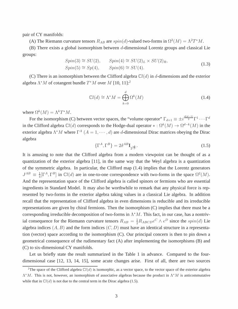
pair of CY manifolds:

(A) The Riemann curvature tensorsRAB arespin(d)-valued two-forms inΩ2(M) = Λ2T ∗M .

(B) There exists a global isomorphism betweend-dimensional Lorentz groups and classical Lie

groups:Spin(3) ∼= SU(2), Spin(4) ∼= SU(2)L × SU(2)R,

Spin(5) ∼= Sp(4), Spin(6) ∼= SU(4).(1.3)

(C) There is an isomorphism between the Clifford algebraCl(d) in d-dimensions and the exterior

algebraΛ∗M of cotangent bundleT ∗M overM [10, 11]:2

Cl(d) ∼= Λ∗M =d⊕

k=0

Ωk(M) (1.4)

whereΩk(M) = ΛkT ∗M .

For the isomorphism (C) between vector spaces, the “volume operator”Γd+1 ≡ ±id(d−1)

2 Γ1 · · ·Γd

in the Clifford algebraCl(d) corresponds to the Hodge-dual operator∗ : Ωk(M) → Ωd−k(M) in the

exterior algebraΛ∗M whereΓA (A = 1, · · · , d) ared-dimensional Dirac matrices obeying the Dirac

algebra

ΓA,ΓB = 2δABI2[

d2 ] . (1.5)

It is amusing to note that the Clifford algebra from a modern viewpoint can be thought of as a

quantization of the exterior algebra [11], in the same way that the Weyl algebra is a quantization

of the symmetric algebra. In particular, the Clifford map (1.4) implies that the Lorentz generators

JAB ≡ 14[ΓA,ΓB] in Cl(d) are in one-to-one correspondence with two-forms in the space Ω2(M).

And the representation space of the Clifford algebra is called spinors or fermions who are essential

ingredients in Standard Model. It may also be worthwhile to remark that any physical force is rep-

resented by two-forms in the exterior algebra taking valuesin a classical Lie algebra. In addition

recall that the representation of Clifford algebra in even dimensions is reducible and its irreducible

representations are given by chiral fermions. Then the isomorphism (C) implies that there must be a

corresponding irreducible decomposition of two-forms inΛ∗M . This fact, in our case, has a nontriv-

ial consequence for the Riemann curvature tensorsRAB = 12RABCDe

C ∧ eD since thespin(d) Lie

algebra indices(A,B) and the form indices(C,D) must have an identical structure in a representa-

tion (vector) space according to the isomorphism (C). Our principal concern is then to pin down a

geometrical consequence of the rudimentary fact (A) after implementing the isomorphisms (B) and

(C) to six-dimensional CY manifolds.

Let us briefly state the result summarized in the Table 1 in advance. Compared to the four-

dimensional case [12, 13, 14, 15], some acute changes arise.First of all, there are two sources

2The space of the Clifford algebraCl(d) is isomorphic, as a vector space, to the vector space of the exterior algebra

Λ∗M . This is not, however, an isomorphism of associative algebras because the product inΛ∗M is anticommutative

while that inCl(d) is not due to the central term in the Dirac algebra (1.5).

3

of two-forms on an orientable six-dimensional manifoldM . One is of course usual two-forms in

Ω2(M) and the other is the Hodge-dual of four-forms inΩ4(M). The doubling of two-forms is

resonant with the fact that the Lorentz generators in an irreducible spinor representation are given by

JAB± ≡ 1

2(I8 ± Γ7)J

AB. Definitely they correspond to the mixture of two-forms and four-forms in

Λ∗M according to the correspondence(Γ7 ↔ ∗). Since we need to take an irreducible representation

of Lorentz symmetry, this demands us to think of the irreducible components of Riemann curvature

tensors as a sum of the usual curvature tensorsRAB and dual curvature tensors defined byRAB ≡(∗G)AB = dωAB + ωAC ∧ ωCB whereGAB is a 4-form tensor taking values inspin(6) ∼= su(4) Lie

algebra [15]. Moreover it is necessary to impose the torsion-free conditions for both spin connections,

ωAB andωAB, which leads to the symmetry property,RCDAB = RABCD andRCDAB = RABCD, of

the curvature tensors. As a result, the Hodge duality admitstwo independent types of curvature tensors

(RABCD ⊕ RABCD) and they have to be decomposed according to the irreducible representation of

spin(6) ∼= su(4) Lie algebra. In the end, the duplication of curvature tensors leads to the doubling

for the variety of six-dimensional spin manifolds.

It should be stressed that the doubling of six-dimensional spin manifolds is an inevitable conse-

quence of the above elementary facts (A,B,C). It may be instructive to apply the foregoing proposi-

tions (A,B,C) to four-manifolds to grasp their significance[13, 14, 15] although the four-dimensional

situation is in stark contrast to the six-dimensional case.See section 6 for a comparison between four

and six dimensions. In four dimensions, the Lorentz groupSpin(4) is isomorphic toSU(2)L ×SU(2)R whosesu(2)L,R Lie algebras consist of irreducible Lorentz generatorsJAB

± ≡ Γ±JAB

with Γ± = 12(I4 ± Γ5) for chiral and anti-chiral representations. The splittingof the Lie algebra,

spin(4) ∼= su(2)L ⊕ su(2)R, is precisely isomorphic to the canonical decomposition ofthe vector

spaceΩ2(M) of two-forms:

Ω2(M) = Ω2+(M)⊕ Ω2

−(M) (1.6)

whereΩ2±(M) ≡ P±Ω

2(M) andP± = 12(1 ± ∗). That is, the six-dimensional vector spaceΩ2(M)

of two-forms splits canonically into the sum of three-dimensional vector spaces of self-dual and

anti-self-dual two-forms. One can apply the canonical splittings in (B) and (C) to the fact (A) si-

multaneously. It results in the well-known decomposition of the curvature tensorR into irreducible

components [16, 17], schematically given by

R =

(W+ + 1

12s B

BT W− + 112s

)(1.7)

wheres is the scalar curvature,B is the traceless Ricci tensor, andW± are the (anti-)self-dual Weyl

tensors. An important lesson from the four-dimensional example is that the irreducible (chiral) rep-

resentation of Lorentz symmetry corresponds to the canonical split (1.6) of two-forms with the pro-

jection operatorP± = 12(1 ± ∗). We observe that the same analysis in six dimensions brings about a

more dramatic result due to the fact6 = 2 + 4. The doubling of six-dimensional spin manifolds will

be important to understand why a CY manifold arises with a mirror pair.

4

The gauge theory formulation of six-dimensional spin manifolds leads to a valuable perspective

for the doubling. The first useful access is to identify a gauge theory object corresponding to a

CY 3-fold in the same sense that a CY 2-fold (or a hyper-Kahler manifold) can be identified with

an SU(2) Yang-Mills instanton in four dimensions [12, 13, 14]. An obvious guess goes toward a

six-dimensional generalization of the four-dimensional Yang-Mills instantons known as Hermitian

Yang-Mills (HYM) instantons. Indeed this identification has been well-known to string theorists and

mathematicians under the name of the Donaldson-Uhlenbeck-Yau (DUY) theorem [18]. We quote a

paragraph in [19] (211 page) to clearly summarize this picture.

The point of intersection between the Calabi conjecture andthe DUY theorem is the

tangent bundle. And here’s why: Once you’ve proved the existence of CY manifolds, you

have not only those manifolds but their tangent bundles as well, because every manifold

has one. Since the tangent bundle is defined by the CY manifold, it inherits its metric

from the parent manifold (in this case, the CY). The metric for the tangent bundle, in

other words, must satisfy the CY equations. It turns out, however, that for the tangent

bundle, the Hermitian Yang-Mills equations are the same as the CY equations, provided

the background metric you’ve selected is the CY. Consequently, the tangent bundle, by

virtue of satisfying the CY equations, automatically satisfies the Hermitian Yang-Mills

equations, too.

If a CY manifoldM can be identified with a HYM instanton, a natural question immediately

arises. Since a CY manifoldM exists with a mirror pair, there will be a mirror CY manifoldM

obeying the mirror relationh1,1(M) = h2,1(M), h2,1(M) = h1,1(M). This in turn implies that

there must be amirror HYM instanton which can be identified with the mirror CY manifold M .

Thus we want to understand the relation between the HYM instanton and its mirror instanton from

the gauge theory perspective. Since the groupSpin(6) is isomorphic toSU(4), the chiral and anti-

chiral representations4 and4′ of Spin(6) are equivalent to the fundamental and anti-fundamental

representations4 and4 of SU(4). Recall that the fundamental representation4 of SU(4) is a complex

representation and so its complex conjugate4 is an inequivalent representation different from4.

Therefore, given a CY manifoldM , one can embed a HYM instanton inherited fromM into two

different representations. But this situation is equally true for the mirror CY manifoldM . In sum,

there is a similar doubling for the variety of HYM instantonsas occurred to CY manifolds.

It may be interesting to compare this situation with the four-dimensional case [14, 15]. In four

dimensions, the positive and negative chirality spinors ofSpin(4) are given bySU(2)L andSU(2)R

spinors,2L and2R, respectively. In this case, it is necessary to have two independentSU(2) factors

to be resonant with the splitting (1.6) because the irreducible representation ofSU(2) is real. It is

interesting to see how (A,B,C) take part in the conspiracy. Consequently, anSU(2)L instanton and a

CY 2-fold live in the chiral vector space2L, while anSU(2)R anti-instanton and a mirror CY 2-fold

live in the anti-chiral vector space2R. In this correspondence, theSU(2) gauge group of Yang-Mills

5

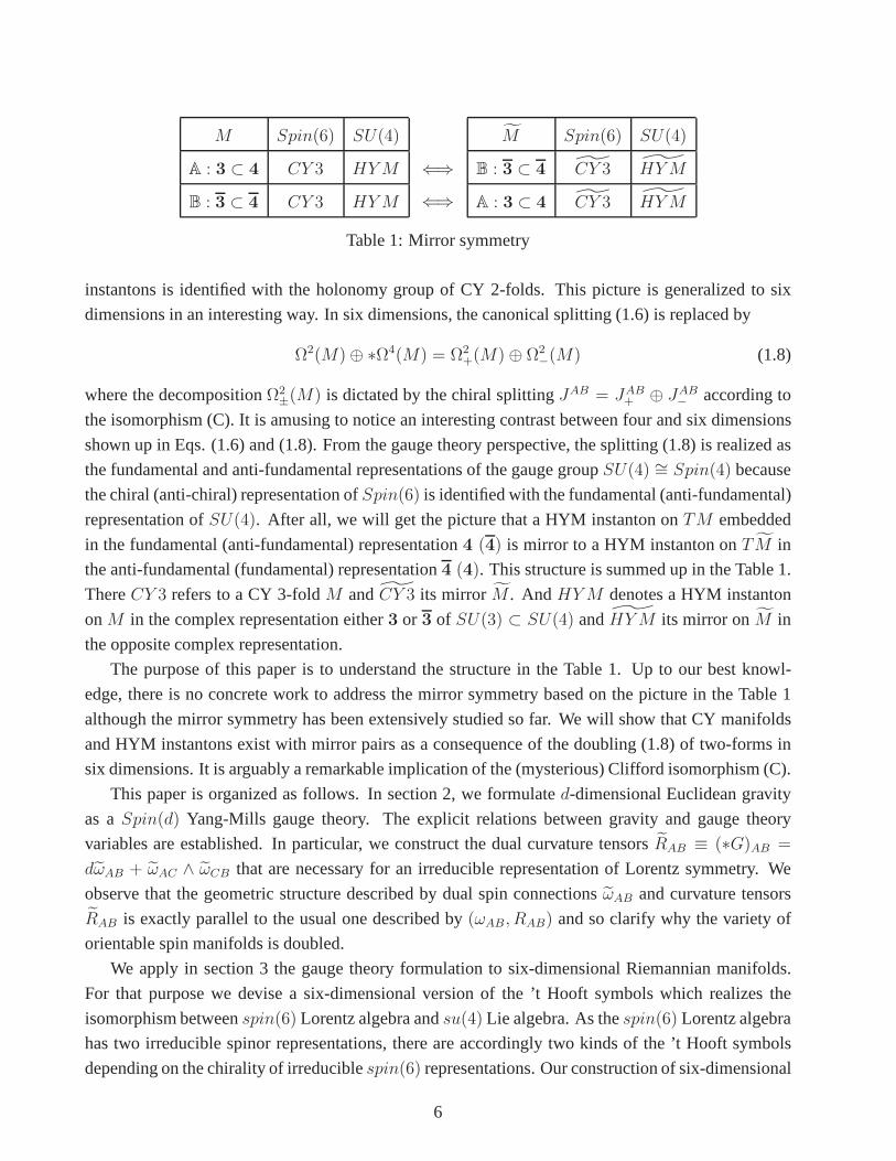
M Spin(6) SU(4)

A : 3 ⊂ 4 CY 3 HYM

B : 3 ⊂ 4 CY 3 HYM

⇐⇒⇐⇒

M Spin(6) SU(4)

B : 3 ⊂ 4 CY 3 HYM

A : 3 ⊂ 4 CY 3 HYM

Table 1: Mirror symmetry

instantons is identified with the holonomy group of CY 2-folds. This picture is generalized to six

dimensions in an interesting way. In six dimensions, the canonical splitting (1.6) is replaced by

Ω2(M)⊕ ∗Ω4(M) = Ω2+(M)⊕ Ω2

−(M) (1.8)

where the decompositionΩ2±(M) is dictated by the chiral splittingJAB = JAB

+ ⊕ JAB− according to

the isomorphism (C). It is amusing to notice an interesting contrast between four and six dimensions

shown up in Eqs. (1.6) and (1.8). From the gauge theory perspective, the splitting (1.8) is realized as

the fundamental and anti-fundamental representations of the gauge groupSU(4) ∼= Spin(4) because

the chiral (anti-chiral) representation ofSpin(6) is identified with the fundamental (anti-fundamental)

representation ofSU(4). After all, we will get the picture that a HYM instanton onTM embedded

in the fundamental (anti-fundamental) representation4 (4) is mirror to a HYM instanton onTM in

the anti-fundamental (fundamental) representation4 (4). This structure is summed up in the Table 1.

ThereCY 3 refers to a CY 3-foldM andCY 3 its mirror M . And HYM denotes a HYM instanton

onM in the complex representation either3 or 3 of SU(3) ⊂ SU(4) andHYM its mirror onM in

the opposite complex representation.

The purpose of this paper is to understand the structure in the Table 1. Up to our best knowl-

edge, there is no concrete work to address the mirror symmetry based on the picture in the Table 1

although the mirror symmetry has been extensively studied so far. We will show that CY manifolds

and HYM instantons exist with mirror pairs as a consequence of the doubling (1.8) of two-forms in

six dimensions. It is arguably a remarkable implication of the (mysterious) Clifford isomorphism (C).

This paper is organized as follows. In section 2, we formulate d-dimensional Euclidean gravity

as aSpin(d) Yang-Mills gauge theory. The explicit relations between gravity and gauge theory

variables are established. In particular, we construct thedual curvature tensorsRAB ≡ (∗G)AB =

dωAB + ωAC ∧ ωCB that are necessary for an irreducible representation of Lorentz symmetry. We

observe that the geometric structure described by dual spinconnectionsωAB and curvature tensors

RAB is exactly parallel to the usual one described by(ωAB, RAB) and so clarify why the variety of

orientable spin manifolds is doubled.

We apply in section 3 the gauge theory formulation to six-dimensional Riemannian manifolds.

For that purpose we devise a six-dimensional version of the ’t Hooft symbols which realizes the

isomorphism betweenspin(6) Lorentz algebra andsu(4) Lie algebra. As thespin(6) Lorentz algebra

has two irreducible spinor representations, there are accordingly two kinds of the ’t Hooft symbols

depending on the chirality of irreduciblespin(6) representations. Our construction of six-dimensional

6

’t Hooft symbols is new up to our best knowledge. Using this construction, we impose the Kahler

condition on the ’t Hooft symbols. This is done by projectingthe ’t Hooft symbols toU(3)-valued

ones and so results in the reduction of the gauge group fromSU(4) to U(3). After imposing the

Ricci-flat condition, the gauge group in Yang-Mills gauge theory is further reduced toSU(3). This

result is utilized to show that six-dimensional CY manifolds are equivalent to HYM instantons in

SU(3) Yang-Mills gauge theory. We elucidate why the irreducible representation of six-dimensional

spin manifolds according to the Lorentz symmetry requires acanonical splitting of them into two

classes depending on their chirality. It turns out that thissplitting is equally applied to CY manifolds

as well as HYM instantons as shown in the Table 1.

In section 4, we apply the results in section 3 to CY manifoldsto see how the mirror symmetry

between them arises from the doubling for the variety of six-dimensional spin manifolds. First we

explore the topological property of CY manifolds by constructing cohomology classes in each chiral

representation. We show that the complex structure deformations byH2,1 cohomology classes in

the positive (negative) chiral representation are isomorphic to the Kahler structure deformations by

H1,1 cohomology classes in the negative (positive) chiral representation. We also demonstrate that

it is always possible to find a pair of CY manifolds such that their Euler characteristics in different

chiral representation have an opposite sign consistent with the mirror symmetry. Since the sign flip

of the Euler characteristics of CY manifolds can definitely be explained by the mirror relation (1.1),

it implies that a pair of CY manifolds in the positive and negative chiral representations is mirror to

each other as indicated by the arrow(⇐⇒) in the Table 1.

In section 5, we revisit the relation between CY manifolds and HYM instantons to discuss the

mirror symmetry between CY manifolds from a completely gauge theory perspective. We show that

a pair of HYM instantons embedded in different complex representations4 and4 corresponds to a

mirror pair of CY manifolds as summarized in the Table 1. Thisresult is consistent with the mirror

symmetry because the integral of the third Chern classc3(E) for a gauge bundleE is equal to the

Euler characteristic of tangent bundleTM whenE = TM . It is due to the fact that the third Chern

class has a desired sign flip between a complex vector bundleE in the fundamental representation

4 and its conjugate bundleE in the anti-fundamental representation4. Therefore we confirm the

picture in the Table 1 that CY manifolds in the classA (B) are equivalent to HYM instantons in the

same classA (B) from the gauge theory formulation and the mirror symmetry between CY manifolds

defined by the arrow(⇐⇒) can be understood as a mirror pair of HYM instantons between inverted

classes in holomorphic vector bundles.

Finally we recapitulate in section 6 the results obtained inthis paper and conclude the paper with

a few speculative remarks.

In appendix A, we fix the basis for the chiral representation of Spin(6) and the fundamental

representation ofSU(4) and list their structure constants. In appendix B, we present an explicit

matrix representation of the six-dimensional ’t Hooft symbols and their algebraic properties in each

chiral basis.

7

2 Gravity As A Gauge Theory

In this section we consider the irreducible spinor representation and the gauge theory formulation

of Riemannian manifolds [14, 15]. This section is to establish the notation for the doubled variety

of Riemannian manifolds, but more detailed exposition willbe deferred to next section. On a Rie-

mannian manifoldM of dimensiond, the spin connection is aspin(d)-valued one-form and can be

identified, in general, with aSpin(d) gauge field. In order to make an explicit identification between

the spin connections and the corresponding gauge fields, letus first consider thed-dimensional Dirac

algebra (1.5) whereΓA (A = 1, · · · , d) are Dirac matrices. Then theSpin(d) Lorentz generators are

given by

JAB =1

4[ΓA,ΓB] (2.1)

which satisfy the following Lorentz algebra

[JAB, JCD] = −(δACJBD − δADJBC − δBCJAD + δBDJAC

). (2.2)

The spin connection is defined by= 12ABJ

AB, which transforms in the standard way as aSpin(d)

gauge field under local Lorentz transformations

→ ′ = ΛΛ−1 + ΛdΛ−1 (2.3)

whereΛ = e12λAB(x)JAB ∈ Spin(d).

In even dimensions, the spinor representation is reducibleand its irreducible representations are

given by positive and negative chiral representations. In next section we will provide an explicit chiral

representation for the six-dimensional case. The Lorentz generators for the chiral representation are

given by

JAB =

(JAB+ 0

0 JAB−

)(2.4)

whereJAB± = Γ±J

AB andΓ± = 12

(I2[

d2 ] ± Γd+1

). Therefore the spin connection in the chiral repre-

sentation takes the form

=1

2ABJ

AB =

(ω(+) 0

0 ω(−)

)=

1

2

(ω(+)ABJ

AB+ 0

0 ω(−)ABJ

AB−

). (2.5)

Here we used a sloppy notation for which must be understood as = 12ABJ

AB whereA =

(A,A′), B = (B,B′) andAB′ = A′B = 0. For a notational simplicity we will use this nota-

tion since it will not introduce too much confusion. It is convenient to introduce the inverted spin

connection which takes the form

=1

2ABJ

AB =

(ω(+) 0

0 ω(−)

)=

1

2

(ω(−)ABJ

AB+ 0

0 ω(+)ABJ

AB−

). (2.6)

8

These spin connections and will be linked via the torsion-free condition, as will be shown

later. As will be explained in next section, the spin connectionsω(+) andω(−) are considered to be

independent and resulted from the doubling of one-forms dueto the Hodge duality in six dimensions.

Now we introduce aSpin(d) gauge field defined by

A = AaTa =

(A(+)aT a 0

0 A(−)a(T a)∗

)(2.7)

whereA(±)a = A(±)aM dxM (a = 1, · · · , d(d−1)

2) are connection one-forms onM . The Lie algebra

generatorsTa =

(T a 0

0 (T a)∗

)∈ spin(d) are matrices obeying the commutation relation

[Ta,Tb] = −fabcTc (2.8)

whereT a and(T a)∗ are generators in a representationR and its conjugate representationR, respec-

tively. The identification we want to make is then given by

=1

2ABJ

AB ∼= A = AaTa. (2.9)

It also leads to the corresponding identification for the spin connection which reads as ∼= A =

AaTa with A(+)a = A(−)a andA(−)a = A(+)a. We will adopt the identification (2.9) by applying the

group isomorphism (1.3). Then the Lorentz transformation (2.3) can be translated into a usual gauge

transformation

A → A′ = ΛAΛ−1 + ΛdΛ−1 (2.10)

whereΛ = eλa(x)Ta ∈ Spin(d). The Riemann curvature tensor is defined by [9]

R =1

2RABJ

AB = d + ∧ =1

2

(dAB +AC ∧CB

)JAB

=1

2

(R

(+)ABJ

AB+ 0

0 R(−)ABJ

AB−

), (2.11)

whereR(±)AB = 1

2

(∂Mω

(±)NAB − ∂Nω

(±)MAB + ω

(±)MACω

(±)NCB − ω

(±)NACω

(±)MCB

)dxM ∧ dxN . Or, in terms of

gauge theory variables, it is given by

F = F aTa = dA+ A ∧ A =(dAa − 1

2fbc

aAb ∧ Ac)Ta

=1

2

(F (+)aT a 0

0 F (−)a(T a)∗

), (2.12)

whereF (±)a = 12

(∂MA

(±)aN − ∂NA

(±)aM − fabcA

(±)bM A

(±)cN

)dxM ∧ dxN .

9

As we outlined in section 1, in addition to the usual curvature tensorRAB = dωAB + ωAC ∧ ωCB,

we need to introduce the dual curvature tensor defined by

RAB ≡ (∗G)AB = dωAB + ωAC ∧ ωCB (2.13)

whereGAB is a(d− 2)-form tensor taking values inspin(d) Lie algebra. One may consider the dual

spin connectionωAB ≡ (∗θ)AB as the Hodge-dual of a(d − 1)-form connectionθAB in spin(d) Lie

algebra. It is useful to introduce the adjoint exterior differential operatorδ : Ωk(M) → Ωk−1(M)

defined by

δ = (−1)dk+d+1 ∗ d∗ (2.14)

where the Hodge-dual operator∗ : Ωk(M) → Ωd−k(M) obeys the well-known relation

∗2 α = (−1)k(d−k)α (2.15)

for α ∈ Ωk(M). Using the adjoint differential operatorδ, thespin(d)-valued four-formGAB in Eq.

(2.13) can be written as

GAB = (−)d−1δθAB + θAC ⊼ θCB (2.16)

where we devised a simplifying notation

α ⊼ β ≡ ∗((∗α) ∧ (∗β)

)∈ Ωp+q−d(M) (2.17)

for α ∈ Ωp(M) andβ ∈ Ωq(M). Using the nilpotency of the adjoint differential operatorδ, i.e.

δ2 = 0, one can derive the (second) Bianchi identity

δGAB + (−)d−1(θAC ⊼ GCB −GAC ⊼ θCB

)= 0. (2.18)

It may be compared to the ordinary Bianchi identity in general relativity which can be written as

follows: dRAB + ωAC ∧ RCB − RAC ∧ ωCB = 0.

Let us introduce dual vielbeinseA ≡ (∗h)A wherehA ∈ Ωd−1(M), in addition to the usual viel-

beinseA (A = 1, · · · , d) which independently form a local orthonormal coframe at each spacetime

point in M . We combine the dual one-formseA with the usual coframeseA to define a matrix of

vielbeins

E =

(0 e(+)AγA

e(−)AγA 0

)(2.19)

where

e(±)A ≡ 1

2(eA ± eA). (2.20)

The coframe basise(±)A ∈ Γ(T ∗M) defines dual vectorsE(±)A = E

(±)MA ∂M ∈ Γ(TM) by a natural

pairing

〈e(±)A, E(±)B 〉 = δAB. (2.21)

10

The above pairing leads to the relatione(±)AM E

(±)MB = δAB. Since we regard the spin connectionsω(+)

andω(−) as independent, let us consider a pair of geometrical data ona spin manifoldM , dubbedA

andB classes, respectively:A :(e(+)A, ω

(+)AB

),

B :(e(−)A, ω

(−)AB

).

(2.22)

We emphasize that the geometric structure of a six-dimensional spin manifold can be described by

either the typeA or the typeB but it will be different from each other even topologically.In other

words, we can separately consider a Riemannian metric for each class given by

ds2± = δABe(±)A ⊗ e(±)B = δABe

(±)AM e

(±)BN dxM ⊗ dxN

≡ g(±)MN(x) dx

M ⊗ dxN (2.23)

or( ∂

∂s

)2±

= δABE(±)A ⊗ E

(±)B = δABE

(±)MA E

(±)NB ∂M ⊗ ∂N

≡ gMN(±) (x) ∂M ⊗ ∂N . (2.24)

In order to recover general relativity from the gauge theory(namely, Cartan’s) formulation of gravity,

it is necessary to impose the torsion-free condition, i.e.,

T (±)A = de(±)A + ω(±)AB ∧ e(±)B = 0. (2.25)

As a result, the spin connections are determined by vielbeins, i.e.ω(±) = ω(±)(e(±)

), from which one

can deduce the first Bianchi identity

R(±)AB ∧ e(±)B = 0 (2.26)

where the curvature tensorsR(±)AB are defined by Eq. (2.11). It is not difficult to deduce from

Eq. (2.26) the symmetry property,R(±)ABCD = R

(±)CDAB, for the Riemann curvature tensorsR(±)

AB ≡12R

(±)ABCDe

(±)C ∧ e(±)D.

If one introduces the torsion matrixT defined by

T = dE+ ∧ E + E ∧ , (2.27)

it is easy to show that

T =

(0 T (+)AγA

T (−)AγA 0

). (2.28)

Therefore the torsion-free condition (2.25) can be succinctly stated asT = 0. It is also straightforward

to show that

dT =1

2

(0 R

(+)AB ∧ e(+)BγA

R(−)AB ∧ e(−)BγA 0

)(2.29)

11

and so the first Bianchi identity (2.26) is automatic becauseof dT = 0. Similarly, using the definition

(2.11), it is easy to derive the second Bianchi identityDR ≡ dR+∧R−R∧ = 0 whose matrix

form is given by

DR =

(D(+)R(+) 0

0 D(−)R(−)

)= 0 (2.30)

where

D(±)R(±) ≡ dR(±) + ω(±) ∧ R(±) − R(±) ∧ ω(±). (2.31)

In terms of gauge theory variables, it can be stated asDF ≡ dF+A∧ F− F∧A = 0 orD(±)F (±) ≡dF (±) + A(±) ∧ F (±) − F (±) ∧ A(±) = 0.

To sum up, ad-dimensional orientable (spin) manifold admits a nowhere vanishing volume form

which brings about an enlargement of the vector spaces for the geometric structure of Riemannian

manifolds through the isomorphism betweenΩk(M) andΩd−k(M). This doubling for the variety of

Riemannian manifolds always happens by the Hodge duality. One is described by(eA, ωAB, RAB)

and the other construction is given by(eA, ωAB, RAB) ∼= (hA, θAB, GAB) which are combined to

give two irreducible representations of Lorentz symmetry for d-dimensional spin manifolds. In next

section we will investigate the irreducible decompositionof six-dimensional spin manifolds under the

Lorentz symmetry to explain why the variety of Riemannian manifolds must be doubled.

3 Spinor Representation of Six-dimensional Riemannian Mani-

folds

We will apply the gauge theory formulation in the previous section to six-dimensional Riemannian

manifolds. For this purpose, theSpin(6) Lorentz group for Euclidean gravity will be identified with

theSU(4) gauge group in Yang-Mills gauge theory. A motivation for thegauge theory formulation

of six-dimensional Euclidean gravity is to identify a gaugetheory object corresponding to a CY

manifold and to understand the mirror symmetry of CY manifolds in terms of Yang-Mills gauge

theory. Because our gauge theory formulation of six-dimensional Riemannian manifolds is based on

the identification (2.9), we will restrict ourselves to orientable six-dimensional manifolds with spin

structure and consider a spinor representation ofSpin(6) in order to scrutinize the relationship.

Let us start with the Clifford algebraCl(6) whose generators are given by

Cl(6) = I8,ΓA,ΓAB,ΓABC ,Γ7ΓAB,Γ7Γ

A,Γ7 (3.1)

whereΓA (A = 1, · · · , 6) are six-dimensional Dirac matrices satisfying the algebra(1.5) andΓA1A2···Ak ≡1k!Γ[A1ΓA2 · · ·ΓAk] assumes the complete antisymmetrization of indices.Γ7 ≡ iΓ1 · · ·Γ6 is the chi-

ral matrix given by (A.4). According to the isomorphism (1.4), the Clifford algebra (3.1) can be

12

isomorphically mapped to the exterior algebra of a cotangent bundleT ∗M

Cl(6) ∼= Λ∗M =6⊕

k=0

Ωk(M) (3.2)

where the chirality operatorΓ7 corresponds to the Hodge dual operator∗ : Ωk(M) → Ω6−k(M).

The spinor representation ofSpin(6) can be constructed by 3 fermion creation operatorsa∗i (i =

1, 2, 3) and the corresponding annihilation operatorsaj (j = 1, 2, 3) (see appendix 5.A in [1]). This

fermionic system can be represented in a Hilbert spaceV of dimension 8 whose states are obtained

by acting the product ofk creation operatorsa∗i1 · · · a∗ik on a Fock vacuum|Ω〉, annihilated by all the

annihilation operators, i.e.,

V =3⊕

k=0

|Ωi1···ik〉 =3⊕

k=0

a∗i1 · · · a∗ik |Ω〉. (3.3)

The spinor representation of the algebra (3.1) is reducibleand has two irreducible spinor represen-

tations. Thus the Hilbert spaceV splits into the spinorsS± of positive and negative chirality, i.e.

V = S+ ⊕ S−, each of dimension 4. If the Fock vacuum|Ω〉 has positive chirality, the positive

chirality spinors ofSpin(6) are states given by

S+ =⊕

k even

|Ωi1···ik〉 = |Ω〉+ |Ωij〉 ≡ 4 (3.4)

while the negative chirality spinors are those obtained by

S− =⊕

k odd

|Ωi1···ik〉 = |Ωi〉+ |Ωijk〉 ≡ 4. (3.5)

As spin(6) Lorentz algebra is isomorphic tosu(4) Lie algebra, the positive and negative chirality

spinors ofspin(6) can be identified with the fundamental representation4 and the anti-fundamental

representation4 of su(4), respectively [1]. As a result, bothSpin(6) andSU(4) have two inequivalent

irreducible representations and the chiral spinor representations onS+ andS− are identified with the

(anti-)fundamental representations4 and4 onC4.

One can form a direct product of the fundamental representations4 and4 of SU(4) in order to

classify the Clifford generators in Eq. (3.1):

4⊗ 4 = 1⊕ 15 = Γ+,ΓAB+ , (3.6)

4⊗ 4 = 1⊕ 15 = Γ−,ΓAB− , (3.7)

4⊗ 4 = 6⊕ 10 = ΓA+,Γ

ABC+ , (3.8)

4⊗ 4 = 6⊕ 10 = ΓA−,Γ

ABC− , (3.9)

whereΓ± ≡ 12(I8±Γ7) are the projection operators onto the space of definite chirality andΓA1A2···Ak

± ≡Γ±Γ

A1A2···Ak . Note that15 in Eqs. (3.6) and (3.7) is the adjoint representation ofSU(4) and6 and

13

10 in Eqs. (3.8) and (3.9) are the antisymmetric and symmetric second-rank tensors ofSU(4), re-

spectively. See appendix A for the Lie algebra generators inthe chiral representation ofSpin(6) and

the fundamental representation ofSU(4). It is important to notice thatΓAB+ ∈ 15 andΓAB

− ∈ 15 are

independent of each other, i.e.[ΓAB+ ,ΓCD

− ] = 0, and this doubling of the Clifford basis is parallel to

the doubling of two-forms according to the Clifford isomorphism (3.2) as will be clarified below.

We want to take an irreducible representation of the Lorentzsymmetry for Riemannian manifolds.

Hence we will refine the identification (2.9) to obtain an irreducible decomposition of curvature ten-

sors under the Lorentz symmetry. As we noticed above, there are two kinds of Lorentz generators

given by the irreducible componentsΓAB± = Γ±Γ

AB which correspond to chiral and anti-chiral repre-

sentations of Lorentz algebraspin(6) ∼= su(4). Compatibly with that purpose, we have already taken

the following split of curvature tensorsRAB = 12RABCDJ

CD:

RAB = R(+)AB ⊕ R

(−)AB =

(F

(+)aAB T a

1 ⊕ F(−)aAB T a

2

)= FAB (3.10)

whereR(±)AB = Γ±RAB and bothT a

1 andT a2 obey thesu(4) Lie algebra defined by (2.8). On the

right-hand side, the doubling ofsu(4) Lie algebra in four-dimensional representationsR1 andR2 was

considered according to the spinor representation on the left-hand side. Since the Lorentz generators

JAB± = Γ±J

AB are in one-to-one correspondence with two-forms in the vector space (1.8), we have

introduced the corresponding two copies of two-forms according to the identification (2.12):

JAB+ ↔ F

(+)AB , JAB

− ↔ F(−)AB . (3.11)

Since the role of the chiral operatorΓ7 is parallel with the Hodge-dual operator∗ : Ωk(M) →Ω6−k(M), the chiral Lorentz generatorsJAB

± = 14(I8 ± Γ7)Γ

AB = 14(ΓAB ∓ i

4!εABCDEFΓ

CDEF )

correspond to a linear combination of two vector spaces, namely,Ω2(M)⊕ ∗Ω4(M). In other words,

the two-formsF (±) = 12F

(±)AB e(±)A ∧ e(±)B in Eq. (3.10) must be understood as elements of the

enlarged vector space, i.e.,

F (±) ∈ Ω2±(M) = Ω2(M)⊕ ∗Ω4(M). (3.12)

As a resultRAB on the left-hand side of Eq. (3.10) has twice as many components as the usual

Riemann curvature tensor. See section 6 for the further exposition of this situation. As we already

discussed in section 1, the correspondence (3.11) implies that thespin(6) ∼= su(4)-valued two-form

R(±)AB = 1

2R

(±)CDABe

(±)C ∧ e(±)D must be regarded as a mixture of two-forms inΩ2(M) and the Hodge-

dual of four-forms inΩ4(M).

In section 2, we have introduced two kinds of Riemann curvature tensorsRAB andRAB = (∗G)AB

where the latter is the dual curvature tensor defined by Eq. (2.13) or (2.16). However it might be

emphasized that the irreducible representation of curvature tensors is given byR(±)AB in Eq. (3.10)

and so the integrability conditions such as the first and second Bianchi identities, Eqs. (2.26) and

(2.31), have been imposed on the combinations rather thanRAB and RAB. The curvature tensors

RAB and RAB may not in general obey the integrability conditions separately. In other words the

14

usual Riemann curvature tensors in general relativity mustbe identified with eitherR(+)AB or R(−)

AB .

Nevertheless one may wonder how the curvature tensor inΩ4(M) obeys the integrability conditions

when the curvature tensor inΩ2(M) identically vanishes. Let us summarize the result in section 2 to

stress how it is achieved. First, we can impose the (dual) torsion-free condition for dual one-forms

eA = (∗h)A and dual spin connectionsωAB = (∗θ)AB wherehA ∈ Ω5(M):

TA = deA + ωAB ∧ eB = 0. (3.13)

Using the form language, the above equation can be written as

TA = δhA − θAB ⊼ hB = 0 (3.14)

whereTA ≡ −(∗T )A ∈ Ω4(M). By solving the above equations, the dual spin connections are

determined by dual vielbeins, i.e.ω = ω(e) or θ = θ(h), from which we can deduce the first Bianchi

identity,RAB ∧ eB = 0 orGAB ⊼ hB = 0.

Suppose thatJAB∗ andT a

∗ are Lie algebra generators in an irreducible representationR∗ of Spin(6)

andSU(4), respectively. Let us then introduceSU(4) gauge fieldsB = BaT a∗ andC = CaT a

∗

identified with the dual spin connectionω = 12ωABJ

AB∗ and the five-form connectionθ = 1

2θABJ

AB∗ ,

respectively, i.e.,

ω =1

2ωABJ

AB∗

∼= B = BaT a∗ , (3.15)

θ =1

2θABJ

AB∗

∼= C = CaT a∗ (3.16)

whereB = ∗C. Then the dual curvature tensors (2.13) and (2.16) are, respectively, written as

F = dB +B ∧B = ∗H, (3.17)

H = (−)d−1δC + C ⊼ C, (3.18)

whereH is a four-form field strength whose Hodge dual is the field strengthF in SU(4) gauge theory.

The integrability condition due to the nilpotency of exterior differentials,d2 = δ2 = 0, immediately

leads to the Bianchi identity

dF +B ∧ F − F ∧B = 0 ⇔ δH + (−)d−1(C ⊼H −H ⊼ C

)= 0. (3.19)

Therefore the geometric structure described by the dual variables(ωAB, RAB) is exactly parallel to

the usual one described by(ωAB, RAB).

It is natural to put the two geometric structures on an equal footing and the irreducible repre-

sentation of the Clifford algebraCl(6) dictates us to identify the curvature tensors in Eq. (3.12) as

follows

F (±) =1

2(F ± F ) =

1

2(F ± ∗H). (3.20)

15

One may note that, on an orientable (spin) manifold, the duplication of curvature tensors always

happens by the Hodge duality. The mixture (3.20) can be understood as follow. One may regard

the Riemann tensorRAB = 12RABCDJ

CD as a linear operator acting on the Hilbert spaceV in Eq.

(3.3). AsRAB contains two gamma matrices, it does not change the chirality of the vector space

V . Therefore, we can represent it in a subspace of definite chirality as eitherR(+)AB : S+ → S+ or

R(−)AB : S− → S−. The former caseR(+)

AB : S+ → S+ takes values in4⊗4 in (3.6) with a singlet being

removed while the latter caseR(−)AB : S− → S− takes values in4 ⊗ 4 in (3.7) with no singlet. Thus

there exist two independent identifications defined by

A :1

2R

(+)ABCDJ

CD+ ≡ F

(+)aAB

(T a ⊕ 0

), (3.21)

B :1

2R

(−)ABCDJ

CD− ≡ F

(−)aAB

(0⊕ (T a)∗

), (3.22)

where the classA (B) lives in the subspaceS+ (S−) of positive (negative) chirality. See appendix

A for explicit chiral representationsJAB± of Spin(6). Because the classesA andB in Eqs. (3.21)

and (3.22) are now represented by4× 4 matrices on both sides, we can take a trace operation for the

matrices which leads to the following relations

A : R(+)ABCD = −F

(+)aAB Tr (T aJCD

+ ) ≡ F(+)aAB ηaCD, (3.23)

B : R(−)ABCD = −F

(−)aAB Tr

((T a)∗JCD

−)≡ F

(−)aAB ηaCD. (3.24)

Here we have introduced a six-dimensional analogue of the ’tHooft symbols defined by

η(±)aAB = −Tr (T a

±JAB± ), (3.25)

where we used a bookkeeping notation,η(+)aAB ≡ ηAB, η

(−)aAB ≡ ηAB andT a

+ ≡ T a, T a− ≡ (T a)∗. An

explicit matrix representation of the six-dimensional ’t Hooft symbols and their algebra are presented

in appendix B.

Note thatF (±)a = 12F

(±)aAB e(±)A ∧ e(±)B in Eqs. (3.21) and (3.22) are the field strengths ofSU(4)

gauge fields. Thus we introduce a pair ofSU(4) gauge fields(A(+), A(−)

)whose field strengths are

given by

F (±) = dA(±) + A(±) ∧A(±). (3.26)

TheSU(4) gauge fieldA(+) (A(−)) is nothing but the spin connection resident in the vector space

S+ (S−) of positive (negative) chirality, i.e.,

ω(±) =1

2ω(±)ABJ

AB±

∼= A(±) = A(±)aT a±. (3.27)

Using Eq. (B.7), one can express the field strengths asF(±)aAB = R

(±)ABCDη

(±)aCD = η

(±)aCD R

(±)CDAB. One

can apply again the same expansion to the index pair[AB] of the Riemann tensorR(±)CDAB. That is,

16

one can expand theSU(4) field strengths in terms of the chiral bases in Eq. (3.25)

A : F(+)aAB = fab

(++)ηbAB, (3.28)

B : F(−)aAB = fab

(−−)ηbAB. (3.29)

As was pointed out in Eq. (3.2), the Clifford algebra (3.1) isisomorphic to the exterior algebraΛ∗M

as vector spaces and so the ’t Hooft symbols in Eq. (3.25) havea one-to-one correspondence with the

basis of two-forms inΩ2±(M) = Ω2(M)⊕∗Ω4(M) depending on the chirality for a given orientation.

Consequently, the six-dimensional Riemann curvature tensors are classified into two classes according

to their six-dimensional chirality:

A : R(+)ABCD = fab

(++)ηaABη

bCD, (3.30)

B : R(−)ABCD = fab

(−−)ηaABη

bCD. (3.31)

Note that the index pairs[AB] and [CD] in the curvature tensorR(±)ABCD have the same chirality

structure because of the symmetry propertyR(±)ABCD = R

(±)CDAB.

The Riemann curvature tensor in six dimensions has225 = 15 × 15 components in total which

is the number of the expansion coefficientsfab(±±) in each class. Because the torsion free condition

has been assumed for the curvature tensors, the first BianchiidentityR(±)A[BCD] = 0 should be imposed

which leads to 120 constraints for each class. After all, thecurvature tensor has105 = 225 − 120

independent components which must be equal to the number of remaining expansion coefficients in

the classA orB after solving the 120 constraints

εABCEFGR(±)DEFG = 0. (3.32)

It is worthwhile to notice that the curvature tensor automatically satisfies the symmetry property

R(±)ABCD = R

(±)CDAB after dictating the first Bianchi identity (3.32). Therefore, one can split the 120

constraints in Eq. (3.32) into105 = 15×142

conditions imposing the symmetryR(±)ABCD = R

(±)CDAB

and extra 15 conditions. These extra conditions can be clarified by considering the tensor product of

SU(4) [20]

15⊗ 15 = (1+ 15+ 20+ 84)S ⊕ (15+ 45+ 45)AS (3.33)

where the first part with 120 components is symmetric and the second part with 105 components is

antisymmetric. It is obvious from our construction thatfab(±±) ∈ 15 ⊗ 15. The 84 components in the

symmetric part is the number of Weyl tensors in six dimensions and the21 = 20 + 1 components

refer to Ricci tensors. The remaining 15 components in the symmetric part are removed by the first

Bianchi identity (3.32) after expelling the antisymmetriccomponents in Eq. (3.33).

One can easily solve the symmetry propertyR(±)ABCD = R

(±)CDAB with the coefficients obeying

fab(++) = f ba

(++), fab(−−) = f ba

(−−), (3.34)

17

which results in 120 components for each chirality and belongs to the symmetric part in Eq. (3.33).

Now the remaining 15 conditions can be removed by the equations

εABCDEFR(±)CDEF = 0. (3.35)

It is obvious that Eq. (3.35) gives rise to nontrivial relations only for the coefficients satisfying Eq.

(3.34). Finally Eq. (3.35) can equivalently be written using Eqs. (B.9) and (B.10) as the 15 constraints

dabcf bc(++) = dabcf bc

(−−) = 0 (3.36)

for each sector. In the end, there remain 105 componentsfab(±±) for each chirality which precisely

match with the independent components of Riemann curvaturetensors in the classA orB.3

Let us introduce the following projection operator acting on 6× 6 antisymmetric matrices defined

by

PABCD± ≡ 1

4

(δACδBD − δADδBC

)± 1

8εABCDEF IEF = PCDAB

± (3.37)

whereI ≡ I3 ⊗ iσ2. Because any6 × 6 antisymmetric matrix of rank 4 spans a four-dimensional

subspaceR4 ⊂ R6, the operator (3.37) in this case can be written in the four-dimensional subspace as

PABCD± ≡ 1

4


)± 1

4εABCD, (A,B,C,D) ∈ R4, (3.38)

and so this case reduces to projection operators for such rank 4 matrices, i.e.,

PABEF± PEFCD

± = PABCD± , PABEF

± PEFCD∓ = 0. (3.39)

Note thatIAB is a6× 6 antisymmetric matrix of rank 6. In this case, the operator (3.37) does not act

as a projection operator but acts as

PABCD± ICD =

(12± 1)IAB. (3.40)

In general, one can deduce by a straightforward calculationthe following properties

PABEF± PEFCD

± = PABCD± +

1

8IABICD, PABEF

± PEFCD∓ = −1

8IABICD. (3.41)

After a little algebra, one can classify the ’t Hooft symbolsin Eq. (3.25) (whose explicit forms

3It may be worthwhile to recall the four-dimensional situation [13, 14]. In four dimensions, the first Bianchi identity

gives rise to 16 constraints. Thus Riemann curvature tensors have20 = 36 − 16 independent components. And the 16

constraints split into 15 ones forRABCD = RCDAB and one more constraint which reads asδabfab

(++) = δabf ab

(−−). The

last constraint is responsible for the equality of the Ricciscalars in the chiral and anti-chiral sectors in Eq. (1.7). The

constraints in Eq. (3.36) correspond to the six-dimensional analogue of the last one.

18

are presented in appendix B) into the eigenspaces of the operator (3.37):

l(+)aAB ≡

η13AB =

i

2λ1 ⊗ σ2, η14AB =

i

2λ2 ⊗ I2,

1√3

(η8AB −

√2η15AB

)= − i

2λ3 ⊗ σ2,

η6AB =i

2λ4 ⊗ σ2, η7AB = − i

2λ5 ⊗ I2, η11AB =

i

2λ6 ⊗ σ2,

η12AB = − i

2λ7 ⊗ I2,

2√3

(− 1

2η3AB +

1√3η8AB +

1√6η15AB

)= − i

2λ8 ⊗ σ2

,(3.42)

m(+)aAB ≡

η1AB =

i

2λ2 ⊗ σ1, η2AB = − i

2λ2 ⊗ σ3, η9AB = − i

2λ5 ⊗ σ1,

η10AB =i

2λ5 ⊗ σ3, η4AB =

i

2λ7 ⊗ σ1, η5AB = − i

2λ7 ⊗ σ3

, (3.43)

n(+)0AB ≡

η3AB +

1√3η8AB +

1√6η15AB =

1

2IAB =

1

2I3 ⊗ iσ2

, (3.44)

wherea, b = 1, · · · , 8 anda, b = 1, · · · , 6 aresu(4) indices in the entries ofl(+)aAB andm(+)a

AB , respec-

tively. They obey the following relations

PABCD− l

(+)aCD = l

(+)aAB , PABCD

+ l(+)aCD = 0,

PABCD− m

(+)aCD = 0, PABCD

+ m(+)aCD = m

(+)aAB ,

PABCD− n

(+)0CD = −1

2n(+)0AB , PABCD

+ n(+)0CD = 3

2n(+)0AB ,

(3.45)

which can be summarized as

PABEF± PEFCD

± = PABCD± +

1

2n(+)0AB n

(+)0CD , PABEF

± PEFCD∓ = −1

2n(+)0AB n

(+)0CD (3.46)

by using the factl(+)aAB n

(+)0AB = m

(+)aAB n

(+)0AB = 0. Of course, Eq. (3.46) is identical to Eq. (3.41).

Similarly, one can also classify the ’t Hooft symbols in Eq. (B.1) into the eigenspaces of the

operator (3.37):

l(−)aAB ≡

−η13AB =

i

2λ1 ⊗ σ2, η14AB =

i

2λ2 ⊗ I2,

1√3

(− η8AB +

√2η15AB

)= − i

2λ3 ⊗ σ2,

−η9AB =i

2λ4 ⊗ σ2, −η10AB = − i

2λ5 ⊗ I2, η4AB =

i

2λ6 ⊗ σ2,

η5AB = − i

2λ7 ⊗ I2,

2√3

(12η3AB +

1√3η8AB +

1√6η15AB

)= − i

2λ8 ⊗ σ2

, (3.47)

m(−)aAB ≡

−η1AB =

i

2λ2 ⊗ σ1, η2AB = − i

2λ2 ⊗ σ3, −η6AB = − i

2λ5 ⊗ σ1,

−η7AB =i

2λ5 ⊗ σ3, η11AB =

i

2λ7 ⊗ σ1, η12AB = − i

2λ7 ⊗ σ3

, (3.48)

n(−)0AB ≡

−η3AB +

1√3η8AB +

1√6η15AB =

1

2IAB =

1

2I3 ⊗ iσ2

. (3.49)

19

The same properties such as Eqs. (3.45) and (3.46) also hold for the above ’t Hooft symbols.

The geometrical meaning of the projection operators in Eq. (3.37) can be understood as follows.

Consider an arbitrary two-form4

F =1

2FMNdx

M ∧ dxN =1

2FABe

A ∧ eB ∈ Ω2(M) (3.50)

and introduce the 15-dimensional complete basis of two-forms inΩ2±(M) = Ω2(M) ⊕ ∗Ω4(M) for

each chirality ofspin(6) Lorentz algebra

Ja+ ≡ 1

2ηaABe

(+)A ∧ e(+)B ∈ Ω2+(M), Ja

− ≡ 1

2ηaABe

(−)A ∧ e(−)A ∈ Ω2−(M). (3.51)

It is easy to derive the following identity using Eqs. (B.9) and (B.10)

Ja± ∧ J b

± ∧ Jc± =

1

2dabcvol

(g(±)

)(3.52)

wherevol(g(±)

)=√

g(±)d6x. The Hodge-dual operation∗ : Ωk(M) → Ω6−k(M) is an isomorphism

of vector spaces which depends upon a metricg(±) and the orientation ofM . The nowhere vanishing

volume forms in (3.52) guarantee that there exists a set of nondegenerate 2-forms onM

Ω± =1

2IABe

(±)A ∧ e(±)B = e(±)1 ∧ e(±)2 + e(±)3 ∧ e(±)4 + e(±)5 ∧ e(±)6. (3.53)

This two-form can be wedged with the Hodge star to construct adiagonalizable operator onΩ2(M)

as follows:

∗Ω±≡ ∗(• ∧ Ω±) : Ω

2(M)•∧Ω±−→ Ω4(M)

∗−→ Ω2(M) (3.54)

by ∗Ω±(α) = ∗(α∧Ω±) for α ∈ Ω2(M). After a little inspection, the15×15 matrix representing∗Ω±

is found to have eigenvalues2, 1 and−1 with eigenspaces of dimension 1, 6 and 8, respectively. On

any six-dimensional orientable Riemannian manifoldM , the space of 2-formsΩ2+(M) in the positive

chirality space can thus be decomposed into three subspaces

Ω2+(M) = Λ2

1 ⊕ Λ26 ⊕ Λ2

8 (3.55)

whereΛ21 andΛ2

6 are locally spanned by

Λ21 = Ω+, (3.56)

Λ26 =

J1+, J

2+, J

4+, J

5+, J

9+, J

10+

, (3.57)

andΛ28 by

Λ28 =

J6+, J

7+, J

11+ , J12

+ , J13+ , J14

+ , K+, L+

(3.58)

4We will indicate the superscript(+) or (−) only when we refer to a quantity belonging to a definite chirality class.

We will often omit the superscript whenever it is not necessary to specify the chirality class.

20

with K+ ≡ 1√3

(J8+−

√2J15

+

)andL+ ≡ 2√

3

(− 1

2J3++

1√3J8++

1√6J15+

). A similar decomposition can be

done with the negative chirality basisJa−. Later we will explain why there exists such a decomposition

of the 15-dimensional vector spaceΩ2±(M).

Note that the entries ofΛ21,Λ

26 andΛ2

8 coincide with those ofn(±)0AB , m

(±)aAB andl(±)a

AB , respectively.

One can quickly see that this coincidence is not an accident.Consider the action of the projection

operator (3.37) on the two-form (3.50) given by

PABCD± FCD =

1

2

(FAB ± 1

4εABCDEFFCDIEF

)(3.59)

or in terms of form notation

2P±F = F ± ∗(F ∧ Ω±) = F ± ∗Ω±F. (3.60)

It is easy to see thatF ∈ Λ28 if P+F = 0 and so it satisfies theΩ-anti-self-duality equation

F = − ∗ (F ∧ Ω±), (3.61)

whereasF ∈ Λ26 = F | P−F = 0 satisfies theΩ-self-duality equation

F = ∗(F ∧ Ω±). (3.62)

It is not difficult to show [2] that the setl(±)aAB , n

(±)0AB

can be identified withu(3) generators which

are embedded inso(6) ∼= su(4). In general, an element ofU(3) group can be represented as

U = exp(i

8∑

a=0

θaλa

)≡ eΘ (3.63)

whereλ0 = I3 is a3×3 unit matrix,λa (a = 1, · · · , 8) are thesu(3) Gell-Mann matrices andθa’s are

real parameters forU to be unitary. The3 × 3 anti-Hermitian matrixΘ consists of matrix elements

which are complex numbersΘij = −(Θji)∗ (i, j = 1, 2, 3) and it can easily be embedded into a

6× 6 real matrix inso(6) ∼= su(4) Lie algebra by replacingΘij = ReΘij + iImΘij by the2× 2 real

matrix ΘAB = I2 · ReΘij + iσ2 · ImΘij. A straightforward calculation (see Eq. (B.17)) shows that

the resulting6× 6 antisymmetric real matrixΘAB can be written as

ΘAB = 2(θ0n

(±)0AB + θal

(±)aAB

)= PABCD

− ΘCD + 3θ0n(±)0AB . (3.64)

Note thatU(3) is the holonomy group of Kahler manifolds. That is, the projection operators in Eq.

(3.37) can serve to project a Riemannian manifold whose holonomy group isSO(6) ∼= SU(4)/Z2 to

a Kahler manifold withU(3) holonomy. It is not difficult to show that it is indeed the case. Suppose

thatM is a complex manifold and let us introduce local complex coordinateszα = x1 + ix2, x3 +

ix4, x5+ ix6, α = 1, 2, 3 and their complex conjugateszα, α = 1, 2, 3, in which an almost complex

structureJ takes the formJαβ = iδαβ, J α

β = −iδαβ [2]. Note that, relative to the real basis

21

xM ,M = 1, · · · , 6, the almost complex structure is given byJ = I = I3 ⊗ iσ2 which we already

introduced in Eq. (3.37). We further impose the Hermitian condition on the complex manifoldM

defined byg(X, Y ) = g(JX, JY ) for anyX, Y ∈ TM . This means that a Riemannian metricg

on a complex manifoldM is a Hermitian metric, i.e.,gαβ = gαβ = 0, gαβ = gβα. The Hermitian

condition can be solved by taking the vielbeins as

eiα = eiα = 0 and Eαi = Eα

i = 0 (3.65)

where a tangent space indexA = 1, · · · , 6 has been split into a holomorphic indexi = 1, 2, 3 and

an anti-holomorphic indexi = 1, 2, 3. This in turn means thatJ ij = iδij , J i

j = −iδ i j . Then one

can see that the two-formΩ± in Eq. (3.53) is a Kahler form, i.e.,Ω±(X, Y ) = g(±)(JX, Y ) and it is

given by

Ω± = ie(±)i ∧ e(±)i = ie(±)iα e

(±)i

βdzα ∧ dzβ = ig

(±)

αβdzα ∧ dzβ (3.66)

wheree(±)i = e(±)iα dzα is a holomorphic one-form ande(±)i = e

(±)iα dzα is an anti-holomorphic one-

form. It is also easy to see that the condition for a Hermitianmanifold (M, g(±)) to be a Kahler

manifold, i.e.dΩ± = 0, is equivalent to the one that the spin connectionω(±)AB is U(3)-valued, i.e.,

ω(±)ij = ω

(±)

ij= 0. (3.67)

Therefore, the spin connections after the Kahler condition (3.67) can be written as the form (3.64).

All the above results can be clearly understood by the properties ofSpin(6) andSU(4) groups.

Introducing complex coordinates onR6 means that one has to consider the Lorentz subgroupU(1)×SU(3) ⊂ SU(4) acting onC3 ⊂ C4 and so one decomposes the4 and4 of SU(4) as4 = 11 ⊕ 3− 1

3

and4 = 1−1⊕3 13

underU(1)×SU(3) where the subscripts denoteU(1) charges. Using the branching

rule ofSU(4) ⊃ U(1)×SU(3) [20], one can get the following decompositions after removingSU(4)

singlets

4⊗ 4− 1 = (3⊗ 3)0 ⊕ (3− 43⊕ 3 4

3) = (8⊕ 1)0 ⊕ (3− 4

3⊕ 3 4

3), (3.68)

4⊗ 4− 1 = (3⊗ 3)0 ⊕ (3− 43⊕ 3 4

3) = (8⊕ 1)0 ⊕ (3− 4

3⊕ 3 4

3). (3.69)

The spin connectionωAB ∈ 15 can be decomposed according to the above branching rule

ωij ∈ 3− 43, ωij ∈ 3 4

3,

ωij − 13δijωkk ∈ 80, ωii ∈ 10.

(3.70)

Hence the Kahler condition (3.67) means that spin connections in3− 43

and3 43

decouple from the

theory and only the components in80 and10 survive. It is now obvious why we could have such

decompositions in Eqs. (3.42)-(3.49) in whichl(±)aAB ∈ 80, m

(±)aAB ∈ (3− 4

3⊕ 3 4

3) andn(±)0

AB ∈ 10.

One can rephrase the Kahler condition (3.67) using the gauge theory formalism. From the identi-

ficationω(±) ≡ Γ± = A(±)aT a± in Eq. (3.27), we get the relation

ω(±)AB = A(±)aη

(±)aAB , A(±)a = −2Tr

(ω(±)T a

±). (3.71)

22

We will focus on the typeA case (with+-chirality) as the same analysis can be applied to the typeB

case (with−-chirality). If (M, g(+)) is a Kahler manifold, Eq. (3.67) means that

A(+)1 = A(+)2 = A(+)4 = A(+)5 = A(+)9 = A(+)10 = 0 (3.72)

becauseηaij 6= 0 only for a = 1, 2, 4, 5, 9, 10, otherwiseηaij = 0. See Eq. (B.17). It should also be

obvious from the branching rule (3.70), i.e.,m(±)aAB ∈ (3− 4

3⊕ 3 4

3). And then theSU(4) structure

constantsfabc in the Table 2 guarantee that the corresponding field strengths also vanish, i.e.,

F (+)a = dA(+)a − 1

2fabcA(+)b ∧A(+)c

=1

2fab(++)η

bABe

(+)A ∧ e(+)B = 0 (3.73)

for a = 1, 2, 4, 5, 9, 10. In other words,A(+)a = 0, f ab(++) = 0 for ∀ b = 1, · · · , 15 and so the gauge

fields take values inU(3) Lie algebra according to the result (3.64). This immediately leads to the

conclusion that

F (+)a = dA(+)a − 1

2fabcA(+)b ∧A(+)c

= fab(++)J

b+ ∈ Λ2

8 ⊕ Λ21 (3.74)

whereF (+)a, a = 0, 1, · · · , 8, are the field strengths ofU(3) gauge fields. As will be shown below,

F (+)0 ∈ Λ21 is the field strength of theU(1) part of the spin connections on a Kahler manifold and

F (+)a ∈ Λ28, a = 1, · · · , 8 belong to theSU(3) part. In particular, asF (+)a ∈ Λ2

8, they satisfy the

Ω-anti-self-duality equation (3.61) known as the HYM equations (or DUY equations) [18]

F (+)a = − ∗ (F (+)a ∧ Ω+), a = 1, · · · , 8. (3.75)

These results are consistent with the branching rule (3.70).

It is well-known [2] that the Ricci-tensor of a Kahler manifold is the field strength of theU(1)

part of the spin connections. Therefore, the Ricci-flat condition corresponds to the resultF (+)0 = 0.

One can explicitly check it as follows. Recall thatF(+)aAB = fab

(++)ηbAB. Using the result (3.72),

one can see that the nonzero components offab(++) run only overa, b = 3, 6, 7, 8, 11, 12, 13, 14, 15.

Thereby the constraint (3.36) becomes nontrivial only for those values. As a result, the number of

independent components offab(++) is given by 9×10

2− 9 = 36. The Ricci-flat conditionR(+)

AB ≡R

(+)ACBC = fab

(++)ηaACη

bBC = 0 further constrains the coefficients. A close inspection shows that out of

21 equations,R(+)AB = 0, only 9 equations are independent and, after utilizing the constraint (3.36),

the equations for the Ricci-flatness can be succinctly arranged as

f 3a(++) +

1√3f 8a(++) +

1√6f 15a(++) = 0. (3.76)

23

The above condition in turn means that

F(+)0AB =

(f 3a(++) +

1√3f 8a(++) +

1√6f 15a(++)

)ηaAB

= F(+)3AB +

1√3F

(+)8AB +

1√6F

(+)15AB = 0. (3.77)

If one introduces a gauge field defined by

A(+)0 ≡ ω(+)ABn

(+)0AB = A(+)3 +

1√3A(+)8 +

1√6A(+)15, (3.78)

one can show that the field strength in Eq. (3.77) is given by

F (+)0 = dA(+)0 (3.79)

after using the fact that theU(3) structure constantsfabc satisfy the following relation

f 3ab +1√3f 8ab +

1√6f 15ab = 0. (3.80)

The relation (3.80) is easy to understand because theU(1) part among theU(3) structure constants

has to vanish. This establishes the result that the Ricci-flatness is equal to the vanishing of theU(1)

field strength. That is,F (+)0 = dA(+)0 ∈ Λ21 has a trivial first Chern class. Again the above result is

consistent with the branching rule (3.70).

In terms of complex coordinates, theU(1) gauge field in Eq. (3.78) on a Kahler manifold is given

by

A(+)0 = iω(+)

ii= −i

(E

(+)αi de(+)i

α − E(+)α

ide

(+)iα

)+ i(E

(+)αi ∂αe

(+)i − E(+)α

i∂αe

(+)i)∈ 10 (3.81)

where the exterior derivative is defined byd = ∂+∂ = dzα∂α+dzα∂α. It is obvious thatA(+)0 cannot

be written as an exact one-form, say,A(+)0 6= dλ with an arbitrary real functionλ(z, z), though it is

closed, i.e.dA(+)0 = 0. Therefore, one can see that theU(1) gauge fieldA(+)0 ∈ 10 is a nontrivial

cohomology element.

In summary, the Kahler condition (3.67) projects the ’t Hooft symbols toU(3)-valued ones in

10 ⊕ 80 and results in the reduction of the gauge group fromSU(4) to U(3). After imposing the

Ricci-flatness, which is equivalent to the conditionF (+)0 = dA(+)0 = 0 ∈ 10, the gauge group is

further reduced toSU(3). Remaining spin connections areSU(3) gauge fields that belong to80

and satisfy the HYM equation (3.75). As a Kahler manifold with the trivial first Chern class is a

CY manifold, this means that the CY condition is equivalent to the HYM equation (3.75) whose

solution is known as HYM instantons [2]. Consequently, we find that six-dimensional CY manifolds

are equivalent to HYM instantons inSU(3) Yang-Mills gauge theory. See the quotation from [19] in

section 1. This equivalence will be more clarified using the gauge theory approach in section 5.

24

The same formulae can be obtained for the typeB case. The Kahler condition (3.67) can similarly

be solved by

A(−)1 = A(−)2 = A(−)6 = A(−)7 = A(−)11 = A(−)12 = 0. (3.82)

The Ricci-flat conditionR(−)AB ≡ R

(−)ACBC = fab

(−−)ηaACη

bBC = 0 leads to the equation

− f 3a(−−) +

1√3f 8a(−−) +

1√6f 15a(−−) = 0. (3.83)

It is equivalent to the vanishing ofU(1) field strength, i.e.F (−)0 = dA(−)0 = 0, where theU(1)

gauge field is defined by

A(−)0 ≡ ω(−)ABn

(−)0AB = −A(−)3 +

1√3A(−)8 +

1√6A(−)15. (3.84)

This fact can be derived by using the fact that theU(3) structure constantsfabc for the typeB case

satisfy the following relation

− f 3ab +1√3f 8ab +

1√6f 15ab = 0 (3.85)

wherea, b now run over3, 4, 5, 8, 9, 10, 13, 14, 15. Note that the entries ofU(3) generators for the

typeB case are different from those for the typeA case. As can be expected, CY manifolds for the

typeB case are also described by the HYM equations

F (−)a = − ∗ (F (−)a ∧ Ω−), a = 1, · · · , 8. (3.86)

4 Mirror Symmetry of Calabi-Yau Manifolds

In this section we want to explore the geometrical properties of six-dimensional Riemannian mani-

folds in the irreducible spinor representationsA andB. In section 2, we have introduced dual vielbeins

eA = (∗h)A and spin connectionsωAB = (∗θ)AB in addition to usual ones(eA, ωAB). The dual ge-

ometric structure described by(eA, ωAB) ∼=(hA, θAB

)is basically generated by the Hodge duality

of the exterior algebraΛ∗M on an orientable manifoldM . According to the chiral structure of irre-

ducible representations in Eqs. (3.6)-(3.9), we have associated two geometric structures(e(+)A, ω

(+)AB

)

and(e(−)A, ω

(−)AB

)on a spin manifoldM where

e(±)A =1

2(e± e)A =

1

2(e± ∗h)A, (4.1)

ω(±)AB =

1

2(ω ± ω)AB =

1

2(ω ± ∗θ)AB. (4.2)

This means that there are two independent ways to model a six-dimensional spin manifold. Accord-

ingly we can consider two kinds of Riemannian manifolds whose metrics are given by

ds2A = e(+)A ⊗ e(+)A, ds2B = e(−)A⊗(−)A, (4.3)

25

whereA andB refer to the chirality class. Each of the metrics defines their own spin connections

ω(±)AB = ω

(±)AB

(e(±)

)through the torsion-free conditions,TA

± = de(±)A + ω(±)AB ∧ e(±)A = 0. Generally

speaking, the variety of six-dimensional spin manifolds issimply doubled due to the Hodge duality

onΛ∗M .

The spin connections can take arbitrary values as far as theysatisfy the integrability condition

(2.26). Their symmetry properties can be characterized by decomposing them into irreducible sub-

spaces underSO(6) group:

ωABC ∈ 6⊗ 15 = ⊗ = ⊕ = 20⊕ 70 (4.4)

where = 20 is a completely antisymmetric part of spin connections defined byω[ABC] =13(ωABC+

ωBCA+ωCAB). In six dimensions, the spin connectionsω[ABC] may be further decomposed as (imag-

inary) self-dual (sd) and anti-self-dual (asd) parts, i.e.,

ω[ABC] =(ωsd[ABC] ∈ 10

)⊕(ωasd[ABC] ∈ 10

). (4.5)

The above decomposition may be shaky because= 20 is already an irreducible representation of

SO(6). It is just for a heuristic comparison with the irreducibleSU(4) representation. Note that6 is

coming from the antisymmetric tensor in4× 4 in Eq. (3.8) or4× 4 in Eq. (3.9). Thus, underSU(4)

group, one can instead get the following decomposition of the spin connections [20]

ωABC ∈ 6⊗ 15 = ⊗ =

(6 =

)⊕(10 =

)⊕(10 =

)⊕(64 =

). (4.6)

Hence notice that the irreducible representation ofSU(4) for spin connections is more refined than

that ofSO(6) and it is identified with the irreduciblespinorrepresentation ofSpin(6).

Introduce a three-form defined by

Ψ(±) ≡ 1

2ω(±)AB ∧ e(±)A ∧ e(±)B = A(±)a ∧ Ja

± (4.7)

where we used the definitions in Eqs. (3.51) and (3.71). Usingthe first Bianchi identity (2.26), one

can show that it satisfies

dΨ(±) = −dA(±)a ∧ Ja± = −1

2A(±)a ∧ dJa

±. (4.8)

One can go further with the identity (4.8). Using the definitionF (±)a = dA(±)a − 12fbc

aA(±)b ∧A(±)c,

the following relation can be derived from Eq. (4.8)

F (±)a ∧ Ja± =

1

2A(±)a ∧D(±)J

a±

= fab(±±)J

a± ∧ J b

± (4.9)

26

whereD(±)Ja± = dJa

± − fbcaA(±)b ∧ Jc

± and the expansionF (±)a = fab(±±)J

b± was used. By writing

ω(±)AB = ω

(±)CABe

(±)C , one can see that

Ψ(±) =1

2ω(±)[ABC]e

(±)A ∧ e(±)B ∧ e(±)C ∈ 10⊕ 10. (4.10)

Also note that

ω(±)ABC =

1

2

(f(±)ABC − f

(±)BCA + f

(±)CAB

)(4.11)

wheref (±)ABC are structure functions defined by the Lie algebra

[E(±)A , E

(±)B ] = −f

(±)AB

CE

(±)C (4.12)

and so they are given by

f(±)AB

C= E

(±)MA E

(±)NB

(∂Me

(±)CN − ∂Ne

(±)CM

). (4.13)

Therefore, the 3-formΨ(±) in Eq. (4.10) can be written as

Ψ(±) =1

4f(±)ABCe

(±)A ∧ e(±)B ∧ e(±)C =1

2de(±)A ∧ e(±)A (4.14)

where we used the structure equations

de(±)A =1

2f(±)BC

Ae(±)B ∧ e(±)C . (4.15)

Finally we arrive at the result

dΨ(±) =1

2de(±)A ∧ de(±)A =

1

8f(±)AB

Ef(±)CDEe

(±)A ∧ e(±)B ∧ e(±)C ∧ e(±)D. (4.16)

Suppose that(M, g(±)) is a Kahler manifold, i.e.dΩ± = dJ0± = 0. On a Kahler manifoldM , the

gauge fieldsA(±)a take values inu(3) Lie algebra, namely, satisfying Eq. (3.72) or (3.82). As was

shown in Eq. (3.70), this means that the spin connections on the Kahler manifold take values only in

10 and80. Thus the three-formΨ(±) can be expanded as

Ψ(±) = A(±)0 ∧ Ω± + A(±)a ∧ J a±. (4.17)

Using the branching rule6 = 3 23⊕ 3− 2

3underSU(3) × U(1), one can identify the surviving spin

connections after the Kahler condition (3.67):

6⊗ 15 →(3 2

3⊕ 3− 2

3

)⊗(10 ⊕ 80

). (4.18)

Consequently the spin connections on the Kahler manifold(M, g(±)) can be decomposed as

ω(±)ABC ∈

(3 2

3⊕ 3− 2

3

)⊕(3 2

3⊗ 80

)⊕(3− 2

3⊗ 80

). (4.19)

27

The first part refers to holomorphic and anti-holomorphicU(1) gauge fields and the remaining parts

describe holomorphic and anti-holomorphicSU(3) gauge fields.

If the three-formΨ(±) is defined on a CY manifoldM , our previous result implies thatΨ(±)0 ≡

43P+Ψ

(±) = A(±)0 ∧ Ω± is a closed 3-form, i.e.dΨ(±)0 = 0.5 This means thatΨ(±)

0 is a nontrivial

element of the third cohomology groupH3(M), becauseA(±)0 cannot be written as an exact one-form

as was pointed out in (3.81) andΩ± is the Kahler form in the second cohomology groupH2(M). It

is obvious from our construction thatΨ(±)0 ∈

(3 2

3⊕ 3− 2

3

)in (4.19) and it is coming from10 =

12 ⊕ 3 23⊕ 6− 2

3and its conjugate10 in (4.10). Therefore it consists of (2,1)- and (1,2)-forms,i.e.,

Ψ(±)0 ∈ H2,1(M)⊕H1,2(M) in the Dolbeault cohomology.

Now let us summarize where the nontrivial classes of Dolbeault cohomology on a CY manifold

come from. We observed that some of them are coming from the metrics in (4.3) and others are

coming from the spin connections in (4.5). It is well-known [2] that a compact Kahler manifold has

a nontrivial second cohomology groupH2(M) which gives rise to a positive Betti numberb2 > 0.

This second cohomology group is coming from the Kahler classΩ± of a Kahler metric defined by Eq.

(3.66). Another nontrivial cohomology class coming from the metric is the holomorphic 3-formΦ±.

A CY 3-fold always admits a globally defined and nowhere vanishing holomorphic volume-formΦ±

satisfying the property [4]

Ω± ∧ Ω± ∧ Ω± = iΦ± ∧ Φ±. (4.20)

Hence the holomorphic 3-formΦ± is basically defined by the metric in (4.3) and forms a one-

dimensional vector bundle called the canonical line bundleL overM . And we have learned that the

remaining cohomology class is coming from the spin connectionΨ(±)0 ∈

(3 2

3⊕ 3− 2

3

)in Eq. (4.17),

which belongs to the third cohomology groupH3(M), to be specific, to the Dolbeault cohomology

H2,1(M)⊕H1,2(M).

The nontrivial cohomology class on a CY manifoldM may be represented as

Ω± = ie(±)i ∧ e(±)i ∈ H1,1(M), (4.21)

Φ± = e(±)i ∧ e(±)j ∧ e(±)k ∈ H3,0(M), Φ± = e(±)i ∧ e(±)j ∧ e(±)k ∈ H0,3(M), (4.22)

Ψ(±)0 = A

(±)0i e(±)i ∧ Ω± ∈ H2,1(M), Ψ

(±)

0 = A(±)0

ie(±)i ∧ Ω± ∈ H1,2(M), (4.23)

wheree(±)i = e(±)iα dzα is a holomorphic one-form ande(±)i = e

(±)iα dzα is an anti-holomorphic one-

form. According to the correspondence (3.2), we define the following map [2]

e(±)i ↔ a(±)i, e(±)i ↔ a(±)∗i , i = 1, 2, 3, (4.24)

wherea(±)i anda(±)∗i are annihilation and creation operators, respectively, acting on the Hilbert space

S± in Eqs. (3.4) and (3.5). Therefore, we identify the cohomology elements in Eqs. (4.21)-(4.23)

5Note that one cannot use Eq. (4.8) to provedΨ(±)0 = 0 because it is no longer true after the projectionP+Ψ

(±). That

is, it is necessary to have bothdA(±)0 = 0 anddΩ± = 0 to verify the closedness.

28

with the following fermion operators with a symmetric ordering prescription

Ω± =1

2

(a(±)∗i a(±)i − a(±)ia

(±)∗i

)=(a(±)∗i a(±)i − 3

2

), (4.25)

Φ± = a(±)ia(±)ja(±)k, Φ± = −a(±)∗i a

(±)∗j a

(±)∗k , (4.26)

Ψ(±)0 = 1

2A

(±)0i (a(±)iΩ± + Ω±a

(±)i) =(a(±)∗j a(±)j − 1

)(A

(±)0i a(±)i

),

Ψ(±)

0 = 12A(±)0i(Ω±a

(±)∗i + a

(±)∗i Ω±) =

(a(±)∗j a(±)j − 2

)(A(±)0ia

(±)∗i

).

(4.27)

Given a metricds2 = eA ⊗ eA, one can determine the spin connectionωAB via the torsion free

condition,TA = deA + ωAB ∧ eB = 0. Because we are dictating an irreducible spinor represen-

tation of local Lorentz symmetry for the identification (2.9), it is necessary to specify which repre-

sentation is chosen to embed the spin connectionωAB. One can equally choose either the positive

or negative chiral representation. This situation may be familiar with supersymmetric solutions in

supergravity. To be specific, consider the supersymmetry transformation of six-dimensional grav-

itino ΨM given byδΨM = DMη where a Dirac operatorDM = ∂M + ωM acts on a chiral spinor

η. Then a background geometry obeyingδΨM = DMη = 0 must satisfy a well-known condition

[DM , DN ]η = 12RMNPQJ

PQη = 0. In this case the representation is determined by an unbroken

supersymmetry generated by the chiral spinorη. Hence the correspondingSU(4) gauge fields are

also identified according to the map (3.27), depending on thechiral representation chosen by the su-

persymmetric background geometry. When a metric is given ina specific chiral representation like

(4.3), one can determine the coefficientsfab(++) in Eq. (3.30) orfab

(−−) in Eq. (3.31) through the ex-

plicit calculation of Riemann curvature tensors. Since thegeometric structures described by the data(e(+)A, ω

(+)AB

)and

(e(−)A, ω

(−)AB

)are completely independent of each other, one can attributethem to

two kinds of metrics.

Hence consider a pair of six-dimensional spin manifolds(M+,M−). There are four ways to assign

the geometric data to the pair because each manifold has two geometric varieties for their residence.

They may be listed as(M+(A),M−(A)), (M+(B),M−(B)), (M+(A),M−(B)), (M+(B),M−(A)).

But the first two cases actually correspond to a single manifold and so we ignore them. Only the last

two cases produce different manifolds and they show up in theTable 1. In general, the Riemannian

manifold described by each metric in the pair will be different even topologically. One can determine

the coefficients(fab(++), f

ab(−−)

)in Eqs. (3.30) and (3.31) for these pairs given their metrics. Since the

pair for the last two cases consists of independent manifolds, it is possible to arrange the coefficients(fab(++), f

ab(−−)

)such that the pair obeys some relation, e.g. Eq. (1.1). We will illustrate later how such

a pair always exists.

Suppose that the spin connections determined by the metricsin (4.3) are embedded into different

chiral representations, as indicated there. And we attribute the metric given byds2A = e(+)A ⊗ e(+)A

embedded in the spinor representation of the typeA to one CY manifoldM+ = M while the metric

ds2B = e(−)A ⊗ e(−)A in the spinor representation of the typeB to the other CY manifoldM− = M .

Then the CY manifoldsM andM will have their own cohomology classes given by Eqs. (4.21)-(4.23)

29

withU(1) gauge fields(A

(+)0i , A(+)0i

)and

(A

(−)0i , A(−)0i

). Therefore, let us consider the cohomology

operators in Eqs. (4.25)-(4.27) for each CY manifold where(+)-operators act on the Hilbert space

S+ in (3.4) and(−)-operators onS− in (3.5). First note thatΦ+S+ = 0, Ψ(+)0 S+ = 0 for the CY

manifoldM andΦ−S− = 0, Ψ(−)

0 S− = 0 for the other CY manifoldM . And the Kahler operator

Ω± in (4.25) assigns the eigenvalue(−32, 12) for the positive-chirality stateS+ = 4 and(−1

2, 32) for

the negative-chirality stateS− = 4. Finally the operatorsΨ(−)0 andΨ

(+)

0 in (4.27) nontrivially act on

S− andS+, respectively, as follows

Ψ(−)0 S− = (a

(−)∗j a(−)j − 1)

[(A

(−)0i a(−)i

)S−

]= (n− − 2)S+, (4.28)

Ψ(+)

0 S+ = (a(+)∗j a(+)j − 2)

[(A(+)0ia

(+)∗i

)S+

]= (n+ − 1)S−, (4.29)

wheren− = (1, 3)(n+ = (0, 2)

)is the occupation number for the stateS− (S+) and we used the

fact that the creation and annihilation operators change the chirality, i.e.,(a(±)∗i , a(±)i

): S± → S∓.

We will see that the above relations imply an important picture about the mirror symmetry of CY

manifolds.

The Euler characteristicχ(M) of a six-dimensional Riemannian manifoldM is defined by

χ(M) =

6∑

r=0

(−)rbr (4.30)

wherebr =∑

p+q=r hp,q(M) is the r-th Betti number. A mirror pair of CY manifolds(M, M)

obeys the propertyhp,q(M) = h3−p,q(M). This property leads to an important result that the Euler

characteristics ofM andM differ exactly by a sign, i.e.,χ(M) = −χ(M ). As a result of the mirror

symmetry, every Calabi-Yau manifold thus has a partner withopposite Euler characteristic. We will

use this fact to identify a mirror CY manifold.

We assumed that the CY manifoldM is of typeA while the other CY manifoldM is of typeB.

Thus the spinor representation ofM (M) is given by the spinor vector spaceS+ = 4 (S− = 4) of

positive (negative) chirality. Recall that we have identified their cohmology classes with the fermion

operators in Eqs. (4.25)-(4.27). If one stares at the results (4.28) and (4.29), one may find that their

structure is very reminiscent of the mirror symmetry in the sense that

ΨB0S− =

(ΩA +

1

2

)S+, Ψ

A

0S+ =(ΩB − 1

2

)S−. (4.31)

The above relation implies that the complex structure deformations byH2,1(M) cohomology classes

in the negative (positive) chiral representation are isomorphic to the Kahler structure deformations by

H1,1(M) cohomology classes in the positive (negative) chiral representation. In particular, consider-

ing the fact thatΩ± andΨ(±)0 are the “quantized” operators of the cohomology classes inH1,1(M)

andH2,1(M), respectively, the map (4.31) implies that the CY manifoldM of typeA is mirror to the

CY manifoldM of typeB. Actually it implies that one can choose the coefficients(fab(++), f

ab(−−)

)in

30

the curvature tensors defined by Eqs. (3.30) and (3.31) such that the Euler characteristics for a pair of

CY manifolds obey the relationχ(M) = −χ(M) and so the mirror relation (1.1).

Every complex vector bundleE of rankn has an underlying real vector bundleER of rank 2n,

obtained by discarding the complex structure on each fiber. Then the top Chern class of a complex

vector bundleE is the Euler class of its realization [21]

cn(E) = e(ER) (4.32)

wheren = rank E. Therefore, the Euler characteristicχ(M) of M for a tangent bundleER = TM

is given by the integral of the top Chern class

χ(M) =

∫

M

cn(E). (4.33)

Recall that ifE is a complex vector bundle, then there exists a dual or conjugate bundleE with an

opposite complex structure whosej-th Chern class is given by [10, 21]

cj(E) = (−1)jcj(E). (4.34)

The Euler characteristicχ(M) for a six-dimensional Riemannian manifoldM is given by

χ(M) ≡ − 1

27 · 3π3

∫

M

εA1A2···A6RA1A2 ∧RA3A4 ∧RA5A6

= − 1

210 · 3π3

∫

M

d6xεM1M2···M6εA1A2···A6RM1M2A1A2RM3M4A3A4RM5M6A5A6 . (4.35)

On one hand, for the typeA in Eq. (3.23) whereR(+)AB = F (+)aηaAB, it is given by

χ+(M) = − 1

27 · 3π3

∫

M

εA1A2···A6R(+)A1A2

∧ R(+)A3A4

∧ R(+)A5A6

= − 1

210 · 3π3

∫

M

(εA1A2···A6ηaA1A2ηbA3A4

ηcA5A6)F (+)a ∧ F (+)b ∧ F (+)c

= − 1

96π3

∫

M

dabcF (+)a ∧ F (+)b ∧ F (+)c (4.36)

where Eq. (B.9) was used. On the other hand, for the typeB in Eq. (3.24) whereR(−)AB = F (−)aηaAB,

the Euler characteristic (4.35) can be written as

χ−(M) =1

27 · 3π3

∫

M

εA1A2···A6R(−)A1A2

∧R(−)A3A4

∧R(−)A5A6

=1

96π3

∫

M

dabcF (−)a ∧ F (−)b ∧ F (−)c (4.37)

31

where Eq. (B.10) was used.6 It is straightforward to represent the above Euler characteristics in terms

of the chiral bases (3.28) and (3.29). For the typeA whereF (+)a = fab(++)J

b+, χ+(M) using the

identity (3.52) reads as

χ+(M) = − 1

192π3

∫

M

d6x√

g(+)dabcddeffad(++)f

be(++)f

cf

(++). (4.38)

Similarly,χ−(M) for the typeB whereF (−)a = fab(−−)J

b− can be written as

χ−(M) =1

192π3

∫

M

d6x√

g(−)dabcddeffad(−−)f

be(−−)f

cf

(−−). (4.39)

Recall that two irreducible spinor representations ofSpin(6) can be identified with the fundamen-

tal and anti-fundamental representations ofSU(4). By choosing a complex structure, e.g., Eq. (3.65),

theSpin(6) tangent bundleTM reduces to aU(3) vector bundleE. In order to utilize the relation

(4.33), let us consider theU(3) ⊂ SU(4) sub-bundleE such thatTM ⊗ C = E ⊕ E. Note that

theU(3) = SU(3) × U(1) subgroup among the Lorentz groupSpin(6) does not mix the creation

and annihilation operators in the Hilbert space (3.3). Thuswe embed the classA in theU(3) vector

bundleE overM . Similarly, by considering the complexificationTM ⊗ C = F ⊕ F , the classB

is embedded in theU(3) vector bundleF overM . It is important to recall that the curvature coeffi-

cientsfab(++) andfab

(−−) are determined by completely independent metricsg(+) onM andg(−) onM ,

respectively. Therefore it is always possible to find a pair of metrics(g(+), g(−)

)such that the Euler

characteristics (4.38) for the typeA and (4.39) for the typeB have a precisely opposite sign, i.e.,

χ+(M) = −χ−(M). As was shown in section 3, the gauge group for a Kahler manifold is reduced to

U(3) and so the structure constantsdabc take values only in theu(3) ⊂ su(4) Lie algebra. For a CY

manifoldM whose holonomy isSU(3) and the structure constantsdabc now take values only in the

su(3) ⊂ u(3) Lie algebra, the Euler characteristicχ(M) is given by [2]

χ(M) = 2(h1,1 − h2,1). (4.40)

Thus the resultχ+(M) = −χ−(M) implies a consistent result with the mirror symmetry (1.1),i.e.,

h1,1(A) = h2,1(B), h1,1(B) = h2,1(A). (4.41)

Note that we cannot flip the sign of Hodge numbers, namely,h1,1(A) = −h1,1(B) andh2,1(A) =

−h2,1(B), because of the definition of the Hodge numberhp,q = dimHp,q(M) ≥ 0. However it

6In order to define the Euler characteristic for the typeB, it is considered that the flip of chirality corresponds to the

parity transformation (see appendix A) and so the orientation reversal. That is the reason for the sign flip ofχ−(M).

But there is some ambiguity for the choice of sign because thesix-dimensional Euler characteristic need not be positive-

definite unlike the four-dimensional case. Hence one may keep the same sign convention forχ−(M) asχ+(M). This

sign ambiguity is insignificant since it can be compensated with the redefinitionR(−)AB

→ −R(−)AB

. In any case the mirror

pair (M, M) will be defined by the conditionχ+(M) = −χ−(M). It is of the essence that the doubling of geometric

variety guarantees the existence of a mirror pair(M, M) such thatχ+(M) = −χ−(M).

32

should be possible to find a pair of CY manifolds obeying the relation (4.41) since the CY manifolds

in the classesA andB are independently constructed. Therefore the mirror relation (4.41) is the only

way to explain the sign flip of the Euler characteristic.

The mirror symmetry (4.41) can be further clarified by using the fact that the Euler characteristic

χ(M) of a spin manifoldM is related to the index of the Dirac operator onM [3]. Denote the Dirac

index for fermion fields in a representationR by index(R). The Euler characteristicχ(M) is then

given by

χ(M) = index(R)− index(R) (4.42)

whereR is the complex conjugate representation ofR. Let 4 be the fundamental representation

of SU(4) and4 its complex conjugate, i.e. the anti-fundamental representation of SU(4). Then

index(4) = −index(4) since in six dimensions the complex conjugation exchanges positive and

negative chirality zero modes while also exchanging4 and4. As SU(3) representations,4 = 1⊕ 3

and4 = 1⊕ 3 whereindex(1) = index(1) = 0 and so the Euler characteristic (4.42) is given by [3]

χ(M) = index(4)− index(4)

= 2 index(4)

= index(3)− index(3)

= 2 index(3). (4.43)

As we observed in Eq. (4.31), the states generated by acting the cohomology classesH1,1(M) and

H2,1(M) on the vector spaceS+ are isomorphic to those generated byH2,1(M) andH1,1(M) acting

on the vector spaceS−. Then the identity (4.43) immediately implies the relationχ+(M) = −χ−(M)

for a pair of spin manifolds embedded in the opposite chirality representations4 and4 (or 3 and3

for CY manifolds). This result is consistent with the mirrorsymmetry (4.41) sinceA ∼= 3 andB ∼= 3.

5 Mirror Symmetry from Gauge Theory

In section 3, the six-dimensional Euclidean gravity has been formulated asSU(4) ∼= Spin(6) Yang-

Mills gauge theory. It was shown that a Kahler manifold is described by the reducedU(3) ⊂ SU(4)

gauge symmetry. After imposing the Ricci-flat condition on the Kahler manifold, the gauge group

in the Yang-Mills theory is further reduced toSU(3). After all, a CY manifold is identified with an

SU(3) HYM instanton from the gauge theory point of view. And the mirror symmetry says that a

CY manifold has a mirror pair satisfying the relation (1.1).Therefore, there must be a corresponding

HYM instanton which can be identified with a mirror CY manifold obeying the mirror relation (4.41).

In this section we will identify the mirror HYM instanton from the gauge theory approach and then

clarify the mirror symmetry between CY manifolds from the gauge theory formulation.

Suppose that the metric of a six-dimensional Riemannian manifold M is given by

ds2 = gMN(x)dxMdxN . (5.1)

33

Let π : E → M be anSU(4) bundle overM whose curvature is defined by

F = dA+ A ∧A

=1

2

(∂MAN − ∂NAM + [AM , AN ]

)dxM ∧ dxN (5.2)

whereA = AaM(x)T adxM is a connection one-form on the vector bundleE. The generatorsT a

of su(4) Lie algebra satisfy the commutation relation (2.8) with a normalizationTrT aT b = −12δab.

ConsiderSU(4) Yang-Mills theory defined on the Riemannnian manifoldM with the metric (5.1)

whose action is given by

SYM = − 1

2g2YM

∫

M

d6x√ggMPgNQTrFMNFPQ. (5.3)

Using the projection operator (3.37) and the identity (3.41), it is easy to derive the following formula

(P±F

)2=

(PA1B1A2B2± FA2B2

)(PA1B1A3B3± FA3B3

)

=1

4

(FA1B1 ±

1

4εA1B1A2B2A3B3FA2B2IA3B3

)2

=1

2FABF

AB ± 1

8εABCDEFFABFCDIEF +

1

8

(IABF

AB)2

= PABCD± FABFCD +

1

8

(IABF

AB)2. (5.4)

One can rewrite the action (5.3) using the above identity as

SYM = − 1

4g2YM

∫

M

d6x√gTr

[(FAB ± 1

4εABCDEFFCDIEF

)2− 1

2

(IABF

AB)2

∓1

2εABCDEFFABFCDIEF

]. (5.5)

The above action can be written in a more compact form as

SYM = − 1

4g2YM

∫

M

d6x√gTr

[(FAB ± ∗(F ∧ Ω

)AB

)2− 1

2

(IABF

AB)2]

± 1

g2YM

∫

M

d6xTrF ∧ F ∧ Ω (5.6)

whereΩ is the two-form of rank 6 defined by Eq. (3.53).

Using the fact

TrF ∧ F = dTr(A ∧ F − 1

3A ∧ A ∧A

)≡ dK, (5.7)

one can see that the last term in Eq. (5.6) is a topological term, i.e.,

TrF ∧ F ∧ Ω = d(K ∧ Ω) (5.8)

34

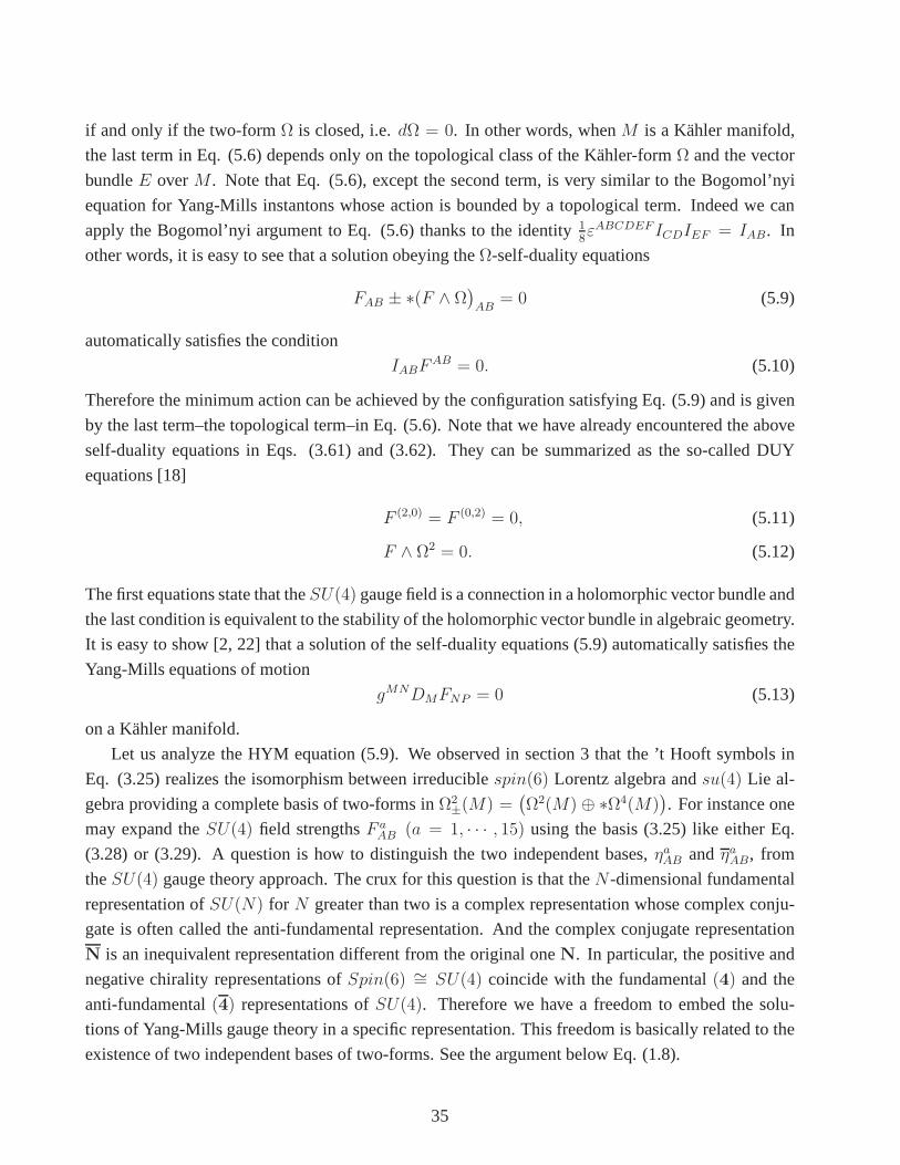
if and only if the two-formΩ is closed, i.e.dΩ = 0. In other words, whenM is a Kahler manifold,

the last term in Eq. (5.6) depends only on the topological class of the Kahler-formΩ and the vector

bundleE overM . Note that Eq. (5.6), except the second term, is very similarto the Bogomol’nyi

equation for Yang-Mills instantons whose action is boundedby a topological term. Indeed we can

apply the Bogomol’nyi argument to Eq. (5.6) thanks to the identity 18εABCDEF ICDIEF = IAB. In

other words, it is easy to see that a solution obeying theΩ-self-duality equations

FAB ± ∗(F ∧ Ω)AB

= 0 (5.9)

automatically satisfies the condition

IABFAB = 0. (5.10)

Therefore the minimum action can be achieved by the configuration satisfying Eq. (5.9) and is given

by the last term–the topological term–in Eq. (5.6). Note that we have already encountered the above

self-duality equations in Eqs. (3.61) and (3.62). They can be summarized as the so-called DUY

equations [18]

F (2,0) = F (0,2) = 0, (5.11)

F ∧ Ω2 = 0. (5.12)

The first equations state that theSU(4) gauge field is a connection in a holomorphic vector bundle and

the last condition is equivalent to the stability of the holomorphic vector bundle in algebraic geometry.

It is easy to show [2, 22] that a solution of the self-duality equations (5.9) automatically satisfies the

Yang-Mills equations of motion

gMNDMFNP = 0 (5.13)

on a Kahler manifold.

Let us analyze the HYM equation (5.9). We observed in section3 that the ’t Hooft symbols in

Eq. (3.25) realizes the isomorphism between irreduciblespin(6) Lorentz algebra andsu(4) Lie al-

gebra providing a complete basis of two-forms inΩ2±(M) =

(Ω2(M) ⊕ ∗Ω4(M)

). For instance one

may expand theSU(4) field strengthsF aAB (a = 1, · · · , 15) using the basis (3.25) like either Eq.

(3.28) or (3.29). A question is how to distinguish the two independent bases,ηaAB andηaAB, from

theSU(4) gauge theory approach. The crux for this question is that theN-dimensional fundamental

representation ofSU(N) for N greater than two is a complex representation whose complex conju-

gate is often called the anti-fundamental representation.And the complex conjugate representation

N is an inequivalent representation different from the original oneN. In particular, the positive and

negative chirality representations ofSpin(6) ∼= SU(4) coincide with the fundamental(4) and the

anti-fundamental(4) representations ofSU(4). Therefore we have a freedom to embed the solu-

tions of Yang-Mills gauge theory in a specific representation. This freedom is basically related to the

existence of two independent bases of two-forms. See the argument below Eq. (1.8).

35

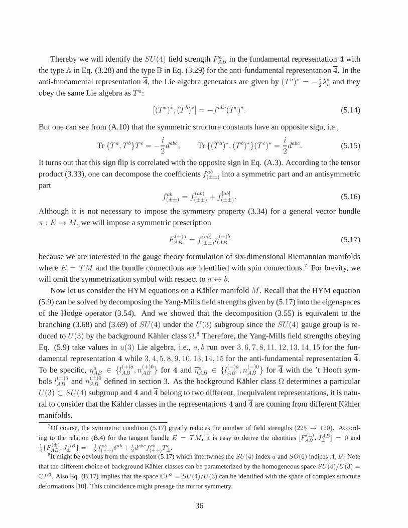
Thereby we will identify theSU(4) field strengthF aAB in the fundamental representation4 with

the typeA in Eq. (3.28) and the typeB in Eq. (3.29) for the anti-fundamental representation4. In the

anti-fundamental representation4, the Lie algebra generators are given by(T a)∗ = − i2λ∗a and they

obey the same Lie algebra asT a:

[(T a)∗, (T b)∗] = −fabc(T c)∗. (5.14)

But one can see from (A.10) that the symmetric structure constants have an opposite sign, i.e.,

Tr T a, T bT c = − i

2dabc, Tr (T a)∗, (T b)∗(T c)∗ =

i

2dabc. (5.15)

It turns out that this sign flip is correlated with the opposite sign in Eq. (A.3). According to the tensor

product (3.33), one can decompose the coefficientsfab(±±) into a symmetric part and an antisymmetric

part

fab(±±) = f

(ab)(±±) + f

[ab](±±). (5.16)

Although it is not necessary to impose the symmetry property(3.34) for a general vector bundle

π : E → M , we will impose a symmetric prescription

F(±)aAB = f

(ab)(±±)η

(±)bAB (5.17)

because we are interested in the gauge theory formulation ofsix-dimensional Riemannian manifolds

whereE = TM and the bundle connections are identified with spin connections.7 For brevity, we

will omit the symmetrization symbol with respect toa ↔ b.

Now let us consider the HYM equations on a Kahler manifoldM . Recall that the HYM equation

(5.9) can be solved by decomposing the Yang-Mills field strengths given by (5.17) into the eigenspaces

of the Hodge operator (3.54). And we showed that the decomposition (3.55) is equivalent to the

branching (3.68) and (3.69) ofSU(4) under theU(3) subgroup since theSU(4) gauge group is re-

duced toU(3) by the background Kahler classΩ.8 Therefore, the Yang-Mills field strengths obeying

Eq. (5.9) take values inu(3) Lie algebra, i.e.,a, b run over3, 6, 7, 8, 11, 12, 13, 14, 15 for the fun-

damental representation4 while 3, 4, 5, 8, 9, 10, 13, 14, 15 for the anti-fundamental representation4.

To be specific,ηaAB ∈ l(+)aAB , n

(+)0AB for 4 andηaAB ∈ l(−)a

AB , n(−)0AB for 4 with the ’t Hooft sym-

bols l(±)aAB andn(±)0

AB defined in section 3. As the background Kahler classΩ determines a particular

U(3) ⊂ SU(4) subgroup and4 and4 belong to two different, inequivalent representations, itis natu-

ral to consider that the Kahler classes in the representations4 and4 are coming from different Kahler

manifolds.7Of course, the symmetric condition (5.17) greatly reduces the number of field strengths(225 → 120). Accord-

ing to the relation (B.4) for the tangent bundleE = TM , it is easy to derive the identities[F (±)AB

, JAB± ] = 0 and

14F

(±)AB

, JAB± = − 1

8fab

(±±)δab + i

2dabcfab

(±±)Tc±.

8It might be obvious from the expansion (5.17) which intertwines theSU(4) indexa andSO(6) indicesA,B. Note

that the different choice of background Kahler classes canbe parameterized by the homogeneous spaceSU(4)/U(3) =

CP 3. Also Eq. (B.17) implies that the spaceCP 3 = SU(4)/U(3) can be identified with the space of complex structure

deformations [10]. This coincidence might presage the mirror symmetry.

36

Hence let us considerSU(4) gauge theories defined on two different CY manifoldsM andM

whose background Kahler classes are, respectively, givenby

Ω+ = n(+)0AB e(+)A ∧ e(+)B , Ω− = n

(−)0AB e(−)A ∧ e(−)B. (5.18)

Given a fixed Kahler class, the HYM equations will be defined by theU(3) gauge theory. The stability

equation (5.10) for each case is then reduced to the following equations

IABF(+)aAB = fab

(++)ηbABIAB = 0 ⇔ f 3a

(++) +1√3f 8a(++) +

1√6f 15a(++) = 0, (5.19)

IABF(−)aAB = fab

(−−)ηbABIAB = 0 ⇔ f 3a

(−−) −1√3f 8a(−−) −

1√6f 15a(−−) = 0. (5.20)

By applying exactly the same argument as section 3, one can conclude that the above equations are

equivalent to the vanishing of the first Chern-class, i.e.,

F (+)0 = dA(+)0 = 0, F (−)0 = dA(−)0 = 0, (5.21)

where theU(1) gauge fieldsA(±)0 are defined by Eqs. (3.78) and (3.84). One can also see from Eq.

(3.61) that theSU(3) basisl(±)aAB definitely picks up the+-sign in Eq. (5.9) and its solution is given

by

F(±)aAB = f ab

(±±)l(±)bAB , a, b = 1, · · · , 8. (5.22)

Consequently we found that the HYM instantons are describedby the reducedSU(3) gauge sym-

metry with the trivial first Chern class. Thus they are precisely SU(3) connections in astableholo-

morphic vector bundle [2]. This is exactly the statement forCY manifolds. Now it becomes clear what

is the mirror relation for HYM instantons. There are two kinds of HYM instantons inSU(4) gauge

theory. One is embedded in the fundamental representation4 and the other is in the anti-fundamental

representation4. Each representation has its own cohomology classes, namely A(+)0 ∈ H1(E,M)

in the first Dolbeault cohomology group with values in the holomorphic vector bundleE overM and

A(−)0 ∈ H1(F , M) with values in the conjugate vector bundleF overM . It should be remarked that

we intend to construct the complex vector bundlesE andF via the tangent bundlesTM⊗C = E⊕E

andTM ⊗ C = F ⊕ F and so the vector bundlesE andF are independent of each other. Since the

positive and negative chiral spinors ofSpin(6) ∼= SU(4) transform as4 and4, one can identify the

representation spaces4 and4 with the spinorsS+ andS−, respectively. Also one can similarly map

the cohomology classes to fermion operators as in Eqs. (4.25)-(4.27). Since the Kahler classΩ±

reduces the gauge group toU(3), it is required to work with theU(3) ⊂ SU(4) subgroup for which

the creation and annihilation operators in the Hilbert space (3.3) are not mixed.

Since we want to understand the mirror symmetry between CY manifolds in terms ofSU(4)

gauge theory, it will be useful to calculate the Chern classes of the vector bundle to elucidate the

mirror symmetry between HYM instantons. We have already shown that the first Chern classc1(E)

of the holomorphic vector bundle satisfying Eq. (5.9) is trivial, i.e. c1(E) = 0. Also we have shown

37

that the last term in Eq. (5.6) is a topological invariant which contains the second Chern classc2(E).

After using Eq. (5.9), one can derive the inequality

− 1

8π2

∫

M±

TrF (±) ∧ F (±) ∧ Ω± ≥ 0, (5.23)

where

c2(V±) = − 1

8π2TrF (±) ∧ F (±) (5.24)

is the second Chern class of a complex vector bundleV+ = E overM+ = M or V− = F over

M− = M . This is known as the Bogomolov inequality [22, 23], which istrue for all stable bundles

with c1(V±) = 0. Using the identification in Eqs. (3.23) and (3.24), one may translate the above

inequality into the one in gravity theory

1

16π2

∫

M±

R(±)AB ∧ R

(±)AB ∧ Ω± ≥ 0. (5.25)

Finally, according to the formula (4.33), we calculate the integral of the third Chern classc3(V±)

given by

χ+(E) = − i

24π3

∫

M

TrF (+) ∧ F (+) ∧ F (+)

= − 1

96π3

∫

M

dabcF (+)a ∧ F (+)b ∧ F (+)c

= − 1

192π3

∫

M

d6x√

g(+)dabcddeffad(++)f

be(++)f

cf

(++) (5.26)

and

χ−(F ) = − i

24π3

∫

M

TrF (−) ∧ F (−) ∧ F (−)

=1

96π3

∫

M

dabcF (−)a ∧ F (−)b ∧ F (−)c

=1

192π3

∫

M

d6x√

g(−)dabcddeffad(−−)f

be(−−)f

cf

(−−). (5.27)

It might be remarked that the relative signc3(F ) = −c3(F ) for the third Chern classes of a complex

vector bundleF and its conjugate bundleF arises from the the property (5.15). Since the complex

vector bundlesE andF are independently defined over two different Kahler manifoldsM andM ,

respectively, the expansion coefficientsfab(±±) in Eq. (5.17) will also be separately determined by

them. Hence it should be possible to construct a pair of complex vector bundles(E → M,F → M)

such thatχ+(E) = −χ−(F ). One may notice that the sign flip in the Euler characteristicis also

consistent with the general result (4.43). Then the above Euler characteristics correctly reproduce the

previous ones for the CY manifoldM and its mirror manifoldM given by Eqs. (4.38) and (4.39).

This constitutes a gauge theory formulation of mirror symmetry.

38

In conclusion we have confirmed the picture depicted in the Table 1 that the mirror symmetry

between CY manifolds can be understood as the existence of mirror pairs of HYM instantons in the

fundamental and anti-fundamental representations3 and3 of SU(3) ⊂ SU(4) gauge symmetry.

6 Discussion

The physics on a curved spacetime becomes more transparent when expressed in a locally inertial

frame and it is even indispensable when one wants to couple spinors to gravity since spinors ind-

dimensions form a representation ofSpin(d) Lorentz group rather thanGL(d,R). Then one can

apply the elementary propositions (A,B,C) in section 1 tod-dimensional Riemannian manifolds to

derive their consequences. It is also required to take an irreducible spinor representation of the

Lorentz symmetry. The upshot, especially, for six-dimensional CY manifolds is rich and interest-

ing. First the proposition A means that Riemann curvature tensorsRABCD carry two kinds of indices;

the first group, say[AB], belongs toSpin(6) indices and the second group[CD] belongs to form

indices inΩ2(M). But the proposition C requires that two groups must have an isomorphic struc-

ture as vector spaces. After imposing the torsion free condition that leads to the symmetry property,

RABCD = RCDAB, the vector space structure for the two groups should be evenidentified. In addition,

the irreducible spinor representation of the Lorentz groupSpin(6) requires us to consider the vector

spacesΩ2(M) andΩ4(M) on an equal footing. The doubling of the vector space(Ω2(M)⊕∗Ω4(M)

)

is resonant with either two independent chiral representations of the Lorentz groupSpin(6) or two

independent complex representations4 and4 of the gauge groupSU(4). We observed that the dou-

bling of vector spaces such as(Ω2(M)⊕∗Ω4(M)

)and(4⊕ 4) essentially brings about the doubling

for the variety of six-dimensional spin manifolds which is responsible for the existence of the mirror

symmetry between CY manifolds.

It may be worthwhile to consider four-dimensional manifolds in perspective. On a four-dimensional

orientable manifold, the vector space of two-formsΩ2(M) is not doubled because the Hodge-dual of

a two-form is again a two-form. Instead the vector spaceΩ2(M) splits canonically into two vector

spaces as (1.6). This split is resonant with the self-duality of chiral Lorentz generatorsJAB± because

they obey the relation

JAB± = ±1

2εABCDJCD

± . (6.1)

Therefore the chiral Lorentz generatorsJAB± have three components only. Combining them together,

they consist of six generators which match with the dimension of Ω2(M). Applying this fact to Eq.

(2.11), one can see thatR(±)AB contains18 = 6 × 3 components and so36 = 18 + 18 components in

total which is the number of components of Riemann curvaturetensorsRABCD before imposing the

first Bianchi identity. This property is in contrast to the six-dimensional case as it has become evident

by comparing Eq. (1.6) with (1.8). An interesting point is that the relations in Eq. (3.45) do not

reduce the number of independent components ofJAB+ and similarlyJAB

− . This should be the case

39

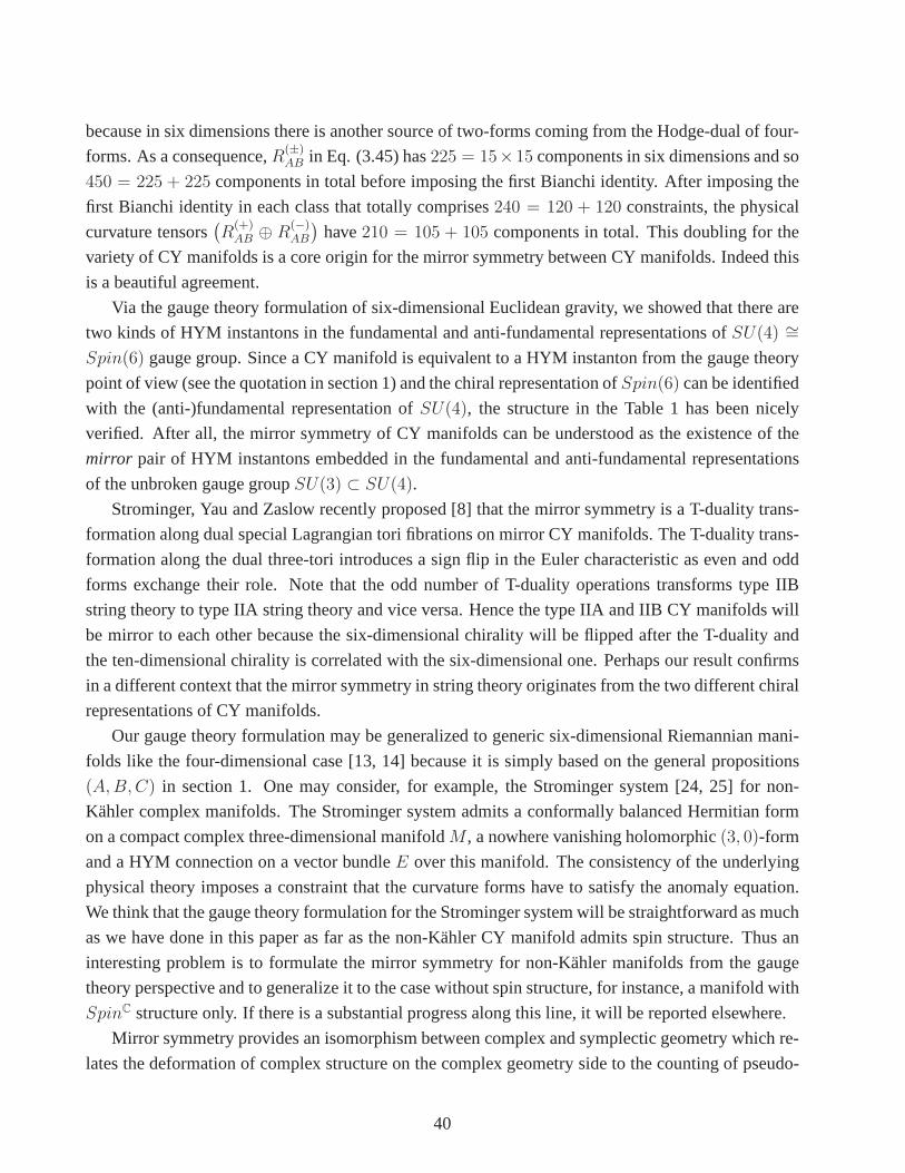
because in six dimensions there is another source of two-forms coming from the Hodge-dual of four-

forms. As a consequence,R(±)AB in Eq. (3.45) has225 = 15×15 components in six dimensions and so

450 = 225 + 225 components in total before imposing the first Bianchi identity. After imposing the

first Bianchi identity in each class that totally comprises240 = 120 + 120 constraints, the physical

curvature tensors(R

(+)AB ⊕ R

(−)AB

)have210 = 105 + 105 components in total. This doubling for the

variety of CY manifolds is a core origin for the mirror symmetry between CY manifolds. Indeed this

is a beautiful agreement.

Via the gauge theory formulation of six-dimensional Euclidean gravity, we showed that there are

two kinds of HYM instantons in the fundamental and anti-fundamental representations ofSU(4) ∼=Spin(6) gauge group. Since a CY manifold is equivalent to a HYM instanton from the gauge theory

point of view (see the quotation in section 1) and the chiral representation ofSpin(6) can be identified

with the (anti-)fundamental representation ofSU(4), the structure in the Table 1 has been nicely

verified. After all, the mirror symmetry of CY manifolds can be understood as the existence of the

mirror pair of HYM instantons embedded in the fundamental and anti-fundamental representations

of the unbroken gauge groupSU(3) ⊂ SU(4).

Strominger, Yau and Zaslow recently proposed [8] that the mirror symmetry is a T-duality trans-

formation along dual special Lagrangian tori fibrations on mirror CY manifolds. The T-duality trans-

formation along the dual three-tori introduces a sign flip inthe Euler characteristic as even and odd

forms exchange their role. Note that the odd number of T-duality operations transforms type IIB

string theory to type IIA string theory and vice versa. Hencethe type IIA and IIB CY manifolds will

be mirror to each other because the six-dimensional chirality will be flipped after the T-duality and

the ten-dimensional chirality is correlated with the six-dimensional one. Perhaps our result confirms

in a different context that the mirror symmetry in string theory originates from the two different chiral

representations of CY manifolds.

Our gauge theory formulation may be generalized to generic six-dimensional Riemannian mani-

folds like the four-dimensional case [13, 14] because it is simply based on the general propositions

(A,B,C) in section 1. One may consider, for example, the Strominger system [24, 25] for non-

Kahler complex manifolds. The Strominger system admits a conformally balanced Hermitian form

on a compact complex three-dimensional manifoldM , a nowhere vanishing holomorphic(3, 0)-form

and a HYM connection on a vector bundleE over this manifold. The consistency of the underlying

physical theory imposes a constraint that the curvature forms have to satisfy the anomaly equation.

We think that the gauge theory formulation for the Strominger system will be straightforward as much

as we have done in this paper as far as the non-Kahler CY manifold admits spin structure. Thus an

interesting problem is to formulate the mirror symmetry fornon-Kahler manifolds from the gauge

theory perspective and to generalize it to the case without spin structure, for instance, a manifold with

SpinC structure only. If there is a substantial progress along this line, it will be reported elsewhere.

Mirror symmetry provides an isomorphism between complex and symplectic geometry which re-

lates the deformation of complex structure on the complex geometry side to the counting of pseudo-

40

holomorphic spheres on the symplectic geometry side. A verysimilar picture arises in emergent

gravity that isomorphically relates the deformations of symplectic structure described by a NCU(1)

gauge theory to the deformations of complex structure in Einstein gravity. The deformation of sym-

plectic structure is represented byF = B + F whereB is an underlying symplectic structure on

M andF = dA is identified with the curvature of line bundleL → M . NC U(1) gauge fields are

introduced via a local coordinate transformationφ ∈ Diff(M) eliminatingU(1) gauge fields, i.e.,

φ∗(F) = B, known as the Darboux theorem in symplectic geometry. It wasclaimed in [26, 27] and

recently shown in [28] that six-dimensional CY manifolds are emergent from NC HermitianU(1)

instantons. Note that the NC HermitianU(1) instanton corresponds by the Seiberg-Witten map to the

U(1) connection in astableholomorphic line bundleL → M [29]. An interesting question imme-

diately arises when we conceive the emergent CY manifolds from the mirror symmetry perspective.

What is the mirror symmetry from the emergent gravity picture ? Emergent gravity implies a very nice

picture for the mirror symmetry. One can consider a nondegenerate four-formC that is co-closed,

i.e., δC = 0. Define a two-formB ≡ ∗C. ThenδC = 0 ⇔ dB = 0. One can equally consider

the deformation of thedual symplectic structureB by an arbitrary closed two-formF ≡ ∗G where

G is a co-closed four-form, i.e.,δG = 0. Then one can introducedual NC U(1) gauge fields by a

local coordinate transformationφ ∈ Diff(M) such thatφ∗(F) = B whereF = B + F = ∗(C +G).

Therefore it should be possible to introducedual NC HermitianU(1) instantons as a solution of the

NC HermitianU(1) equation defined byF = − ∗(˜F ∧ B

)where ˜F = d

Ã − i

Ã ∧ Ã is the field

strength of dual NCU(1) gauge fieldsA. We conjecture that the dual NC HermitianU(1) instanton

is equivalent to adual CY manifold which is certainly mirror to the CY manifold emergent from the

original NC HermitianU(1) instanton. If this conjecture is true, it implies that the mirror symmetry

of CY manifolds is simply the Hodge theory for the deformation of symplectic anddual symplectic

structures. We hope to prove this conjecture soon.

Acknowledgments

We are grateful to Chanju Kim for a collaboration at an early stage and very helpful discussions. HSY

thanks Richard Szabo for his warm hospitality and valuable discussions during his visit to Heriot-Watt

University, Edinburgh. He also thanks Jungjai Lee and John J. Oh for constructive discussions and

collaborations with a related subject. The work of H.S. Yangwas supported by the National Research

Foundation of Korea (NRF) grant funded by the Korea government (MOE) (No. 2011-0010597) and

partially by the National Research Foundation of Korea (NRF) grant funded by the Korea government

(MSIP) (No. 2014R1A2A1A01002306). The work of S. Yun was supported by the World Class

University grant number R32-10130.

41

A Spin(6) and SU(4)

We consider the six-dimensional Clifford algebra with the Dirac matrices given by

ΓA =

(0 γA

γA 0

), A = 1, · · · , 6 (A.1)

whereγA = (γA)†. Thus the Dirac matrices we have taken are Hermitian, i.e.,(ΓA)† = ΓA. We take

(γi)† = γi (i = 1, · · · , 5) and(γ6)† = −γ6. The Lorentz generators for the irreducible (chiral) spinor

representation ofSpin(6) are defined by

JAB± ≡ 1

2(I8 ± Γ7)J

AB (A.2)

whereΓ7 = iΓ1 · · ·Γ6. Note thatJAB+ andJAB

− independently satisfy the Lorentz algebra (2.2) and

commute each other, i.e.,[JAB+ , JCD

− ] = 0. They also satisfy the anti-commutation relation

JAB± , JCD

± = −1

2


)Γ± ± i

2εABCDEFJEF

± . (A.3)

Because the chiral matrixΓ7 is given by

Γ7 =

(I4 0

0 −I4

)(A.4)

whereI4 is a4 × 4 identity matrix, the generators of the chiral spinor representation in Eq. (A.2) are

given by4× 4 matrices. We will use the following representation of Diracmatrices [30]

γ1 =

0 0 0 −1

0 0 1 0

0 1 0 0

−1 0 0 0

, γ2 =

0 0 0 i

0 0 i 0

0 −i 0 0

−i 0 0 0

, γ3 =

0 0 1 0

0 0 0 1

1 0 0 0

0 1 0 0

,

γ4 =

0 0 −i 0

0 0 0 i

i 0 0 0

0 −i 0 0

, γ5 =

1 0 0 0

0 1 0 0

0 0 −1 0

0 0 0 −1

= −γ1γ2γ3γ4, (A.5)

satisfying theSpin(5) Clifford algebra relations

γiγj + γjγi = 2δij, i, j = 1, · · · , 5. (A.6)

Then the two independent chiral spinor representations ofSpin(6) are given by

JAB+ = J ij

+ =1

4[γi, γj ], J i6

+ =i

2γi, (A.7)

JAB− = J ij

− =1

4[γi, γj ], J i6

− = − i

2γi. (A.8)

42

One can check that the generatorsJAB+ andJAB

− separately obey the Lorentz algebra (2.2).

One can exchange the positive-chirality, (A.7), and negative-chirality, (A.8), representations of

Spin(6) by a parity transformation, which is a reflectionxM → −xM of any one element of the

fundamental six-dimensional representation ofSpin(6) [1]; in our case,x6 → −x6. But they cannot

be connected by anySO(6) rotations.

The anti-Hermitian4 × 4 matricesT a = i2λa, a = 1, · · · , 15 with vanishing traces constitute the

basis ofSU(4) Lie algebra. The Hermitian4× 4 matricesλa are given by

λ1 =

0 1 0 0

1 0 0 0

0 0 0 0

0 0 0 0

, λ2 =

0 −i 0 0

i 0 0 0

0 0 0 0

0 0 0 0

, λ3 =

1 0 0 0

0 −1 0 0

0 0 0 0

0 0 0 0

,

λ4 =

0 0 1 0

0 0 0 0

1 0 0 0

0 0 0 0

, λ5 =

0 0 −i 0

0 0 0 0

i 0 0 0

0 0 0 0

, λ6 =

0 0 0 0

0 0 1 0

0 1 0 0

0 0 0 0

,

λ7 =

0 0 0 0

0 0 −i 0

0 i 0 0

0 0 0 0

, λ8 =1√3

1 0 0 0

0 1 0 0

0 0 −2 0

0 0 0 0

, λ9 =

0 0 0 1

0 0 0 0

0 0 0 0

1 0 0 0

,

λ10 =

0 0 0 −i

0 0 0 0

0 0 0 0

i 0 0 0

, λ11 =

0 0 0 0

0 0 0 1

0 0 0 0

0 1 0 0

, λ12 =

0 0 0 0

0 0 0 −i

0 0 0 0

0 i 0 0

,

λ13 =

0 0 0 0

0 0 0 0

0 0 0 1

0 0 1 0

, λ14 =

0 0 0 0

0 0 0 0

0 0 0 −i

0 0 i 0

, λ15 =1√6

1 0 0 0

0 1 0 0

0 0 1 0

0 0 0 −3

.(A.9)

The generatorsT a = i2λa satisfy the following relation

T aT b = −1

8δabI4 −

1

2fabcT c +

i

2dabcT c (A.10)

where the structure constantsfabc are completely antisymmetric whiledabc are symmetric with respect

to all of their indices. Their values are shown in the tables 1and 2. (We get these tables from [31].)

43

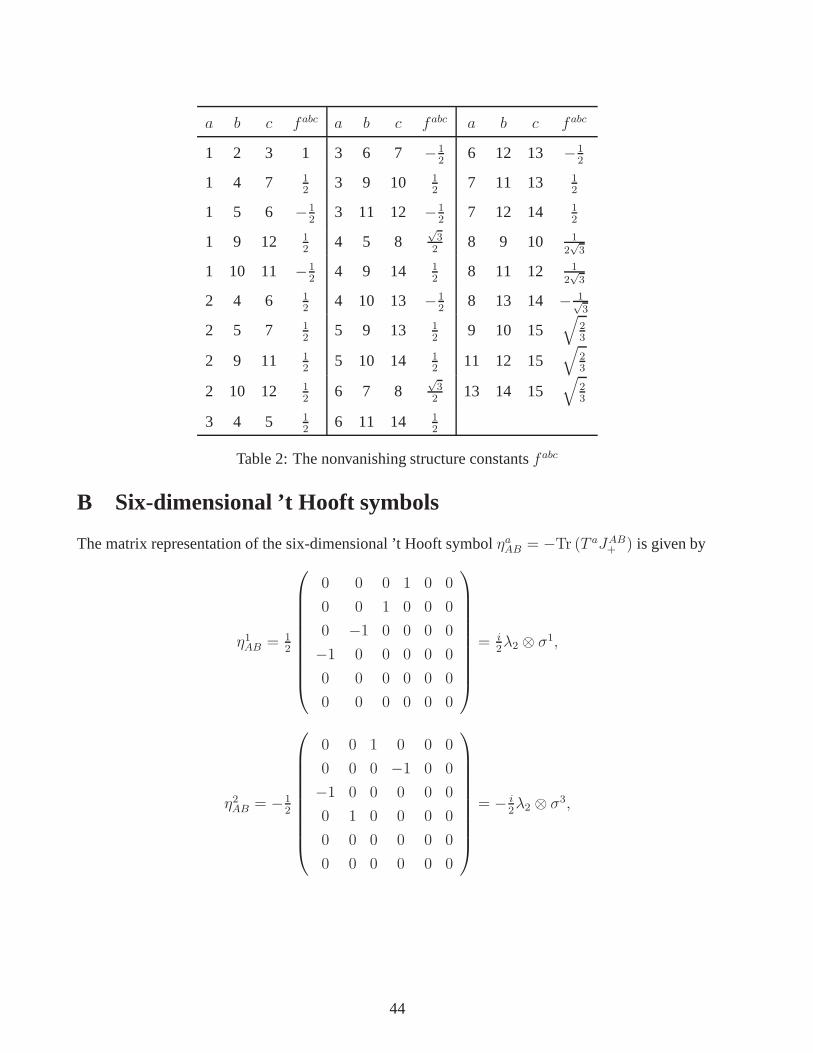
a b c fabc a b c fabc a b c fabc

1 2 3 1 3 6 7 −12

6 12 13 −12

1 4 7 12

3 9 10 12

7 11 13 12

1 5 6 −12

3 11 12 −12

7 12 14 12

1 9 12 12

4 5 8√32

8 9 10 12√3

1 10 11 −12

4 9 14 12

8 11 12 12√3

2 4 6 12

4 10 13 −12

8 13 14 − 1√3

2 5 7 12

5 9 13 12

9 10 15√

23

2 9 11 12

5 10 14 12

11 12 15√

23

2 10 12 12

6 7 8√32

13 14 15√

23

3 4 5 12

6 11 14 12

Table 2: The nonvanishing structure constantsfabc

B Six-dimensional ’t Hooft symbols

The matrix representation of the six-dimensional ’t Hooft symbolηaAB = −Tr (T aJAB+ ) is given by

η1AB = 12

0 0 0 1 0 0

0 0 1 0 0 0

0 −1 0 0 0 0

−1 0 0 0 0 0

0 0 0 0 0 0

0 0 0 0 0 0

= i2λ2 ⊗ σ1,

η2AB = −12

0 0 1 0 0 0

0 0 0 −1 0 0

−1 0 0 0 0 0

0 1 0 0 0 0

0 0 0 0 0 0

0 0 0 0 0 0

= − i2λ2 ⊗ σ3,

44

a b c dabc a b c dabc a b c dabc

1 1 8 1√3

3 9 9 12

7 11 14 −12

1 1 15 1√6

3 10 10 12

7 12 13 12

1 4 6 12

3 11 11 −12

8 8 8 − 1√3

1 5 7 12

3 12 12 −12

8 8 15 1√6

1 9 11 12

4 4 8 − 12√3

8 9 9 12√3

1 10 12 12

4 4 15 1√6

8 10 10 12√3

2 2 8 1√3

4 9 13 12

8 11 11 12√3

2 2 15 1√6

4 10 14 12

8 12 12 12√3

2 4 7 −12

5 5 8 − 12√3

8 13 13 − 1√3

2 5 6 12

5 5 15 1√6

8 14 14 − 1√3

2 9 12 −12

5 9 14 −12

9 9 15 − 1√6

2 10 11 12

5 10 13 12

10 10 15 − 1√6

3 3 8 1√3

6 6 8 − 12√3

11 11 15 − 1√6

3 3 15 1√6

6 6 15 1√6

12 12 15 − 1√6

3 4 4 12

6 11 13 12

13 13 15 − 1√6

3 5 5 12

6 12 14 12

14 14 15 − 1√6

3 6 6 −12

7 7 8 − 12√3

15 15 15 −√

23

3 7 7 −12

7 7 15 1√6

Table 3: The nonvanishing structure constantsdabc

η3AB = 12

0 1 0 0 0 0

−1 0 0 0 0 0

0 0 0 1 0 0

0 0 −1 0 0 0

0 0 0 0 0 0

0 0 0 0 0 0

= i2

(23I3 +

1√3λ8

)⊗ σ2,

45

η4AB = 12

0 0 0 0 0 0

0 0 0 0 0 0

0 0 0 0 0 1

0 0 0 0 1 0

0 0 0 −1 0 0

0 0 −1 0 0 0

= i2λ7 ⊗ σ1,

η5AB = −12

0 0 0 0 0 0

0 0 0 0 0 0

0 0 0 0 1 0

0 0 0 0 0 −1

0 0 −1 0 0 0

0 0 0 1 0 0

= − i2λ7 ⊗ σ3,

η6AB = 12

0 0 0 0 0 1

0 0 0 0 −1 0

0 0 0 0 0 0

0 0 0 0 0 0

0 1 0 0 0 0

−1 0 0 0 0 0

= i2λ4 ⊗ σ2,

η7AB = −12

0 0 0 0 1 0

0 0 0 0 0 1

0 0 0 0 0 0

0 0 0 0 0 0

−1 0 0 0 0 0

0 −1 0 0 0 0

= − i2λ5 ⊗ I2,

η8AB = − 12√3

0 1 0 0 0 0

−1 0 0 0 0 0

0 0 0 −1 0 0

0 0 1 0 0 0

0 0 0 0 0 −2

0 0 0 0 2 0

= − i

2√3

(− 2

3I3 + λ3 +

2√3λ8

)⊗ σ2,

46

η9AB = −12

0 0 0 0 0 1

0 0 0 0 1 0

0 0 0 0 0 0

0 0 0 0 0 0

0 −1 0 0 0 0

−1 0 0 0 0 0

= − i2λ5 ⊗ σ1,

η10AB = 12

0 0 0 0 1 0

0 0 0 0 0 −1

0 0 0 0 0 0

0 0 0 0 0 0

−1 0 0 0 0 0

0 1 0 0 0 0

= i2λ5 ⊗ σ3,

η11AB = 12

0 0 0 0 0 0

0 0 0 0 0 0

0 0 0 0 0 1

0 0 0 0 −1 0

0 0 0 1 0 0

0 0 −1 0 0 0

= i2λ6 ⊗ σ2,

η12AB = −12

0 0 0 0 0 0

0 0 0 0 0 0

0 0 0 0 1 0

0 0 0 0 0 1

0 0 −1 0 0 0

0 0 0 −1 0 0

= − i2λ7 ⊗ I2,

η13AB = 12

0 0 0 1 0 0

0 0 −1 0 0 0

0 1 0 0 0 0

−1 0 0 0 0 0

0 0 0 0 0 0

0 0 0 0 0 0

= i2λ1 ⊗ σ2,

47

η14AB = 12

0 0 1 0 0 0

0 0 0 1 0 0

−1 0 0 0 0 0

0 −1 0 0 0 0

0 0 0 0 0 0

0 0 0 0 0 0

= i2λ2 ⊗ I2,

η15AB = 1√6

0 1 0 0 0 0

−1 0 0 0 0 0

0 0 0 −1 0 0

0 0 1 0 0 0

0 0 0 0 0 1

0 0 0 0 −1 0

= i√6

(13I3 + λ3 − 1√

3λ8

)⊗ σ2,

whereI2 andI3 are two and three dimensional identity matrices, and(σ1, σ2, σ3) are the Pauli matrices

andλa (a = 1, · · · , 8) are theSU(3) Gell-Mann matrices.

The matrix representation of the six-dimensional ’t Hooft symbol ηaAB = −Tr((T a)∗JAB

−)

can

be obtained by flipping a global sign for the entriesa = 1, 3, 4, 6, 8, 9, 11, 13, 15 and a sign flip in the

sixth row and column of the matricesηaAB:

η1AB = − i

2λ2 ⊗ σ1, η2AB = − i

2λ2 ⊗ σ3, η3AB = − i

2

(23I3 +

1√3λ8

)⊗ σ2,

η4AB =i

2λ6 ⊗ σ2, η5AB = − i

2λ7 ⊗ I2, η6AB =

i

2λ5 ⊗ σ1,

η7AB = − i

2λ5 ⊗ σ3, η8AB =

i

2√3

(23I3 + λ3 −

2√3λ8

)⊗ σ2, η9AB = − i

2λ4 ⊗ σ2,

η10AB =i

2λ5 ⊗ I2, η11AB =

i

2λ7 ⊗ σ1, η12AB = − i

2λ7 ⊗ σ3, (B.1)

η13AB = − i

2λ1 ⊗ σ2, η14AB =

i

2λ2 ⊗ I2, η15AB =

i√6

(13I3 − λ3 −

1√3λ8

)⊗ σ2.

In order to derive algebras obeyed by the ’t Hooft symbols, first note that eitherSpin(6) generators

JAB± or SU(4) generatorsT a

+ ≡ T a andT a− ≡ (T a)∗ can serve as a complete basis of any traceless,

Hermitian4× 4 matrixK, i.e.,

K =

15∑

a=1

k±a T

a± =

1

2

6∑

A,B=1

K±ABJ

AB± . (B.2)

Using the definition (3.25), one can easily deduce that

T a± =

1

2η(±)aAB JAB

± , (B.3)

JAB± = 2η

(±)aAB T a

± (B.4)

48

whereη(+)aAB ≡ ηaAB andη(−)a

AB ≡ ηaAB. Then one can consider the following matrix products

I : T a±T

b± =

1

4η(±)aAB η

(±)bCD JAB

± JCD± , (B.5)

II : JAB± JCD

± = 4η(±)aAB η

(±)bCD T a

±Tb±. (B.6)

By applying Eqs. (2.2), (A.3) and (A.10) to the above matrix products, one can easily get the algebras

obeyed by the six-dimensional ’t Hooft symbols:

ηaABηbAB = δab = ηaABη

bAB, (B.7)

ηaABηaCD =

1

2


)= ηaABη

aCD, (B.8)

1

4εABCDEFηaCDη

bEF = dabcηcAB, (B.9)

1

4εABCDEFηaCDη

bEF = dabcηcAB, (B.10)

ηaACηbBC − ηaBCη

bAC = fabcηcAB, (B.11)

ηaACηbBC − ηaBCη

bAC = fabcηcAB, (B.12)

fabcηaABηbCD =

1

2

(δACη

cBD − δADη

cBC − δBCη

cAD + δBDη

cAC

), (B.13)

fabcηaABηbCD =

1

2

(δACη

cBD − δADη

cBC − δBCη

cAD + δBDη

cAC

), (B.14)

dabcηaABηbCD =

1

4εABCDEFηcEF , (B.15)

dabcηaABηbCD =

1

4εABCDEFηcEF . (B.16)

Finally we list the nonzero components of the ’t Hooft symbols in the basis of complex coordinates

zα = z1 = x1 + ix2, z2 = x3 + ix4, z3 = x5 + ix6 and their complex conjugateszα where

α, α = 1, 2, 3. We will denoteηaαβ = ηazαzβ

, ηaαβ

= ηazαzβ

, etc. in the hope of no confusion with the

real basis:

η112 = − i4, η212 = −1

4, η423 = − i

4, η523 = −1

4, η913 =

i4, η1013 = 1

4,

η311 =i4, η322 =

i4, η613 =

i4, η713 = −1

4,

η811 = − i

4√3, η822 =

i

4√3, η833 =

i

2√3, η1123 = i

4, η1223 = −1

4,

η1312 = i4, η1412 = 1

4, η1511 = i

2√6, η1522 = − i

2√6, η1533 = i

2√6.

(B.17)

Here the complex conjugates are not shown up since they can easily be implemented. The cor-

responding values ofηaAB can be obtained from those ofηaAB by flipping a sign for the entries

a = 1, 3, 4, 6, 8, 9, 11, 13, 15 as well as interchangingz3 ↔ z3 for all entries. The above result

implies that the space of complex structure deformations can be identified with the coset space

SU(4)/U(3) = CP 3 [10].

49

References

[1] M. B. Green, J. H. Schwarz and E. Witten,Superstring Theory, Vol. 1, Cambridge Univ. Press,

New York, 1987.

[2] M. B. Green, J. H. Schwarz and E. Witten,Superstring Theory, Vol. 2, Cambridge Univ. Press,

New York, 1987.

[3] P. Candelas, G. T. Horowitz, A. Strominger and E. Witten,Vacuum configurations for super-

strings, Nucl. Phys.B258 (1985) 46.

[4] K. Hori, S. Katz, A. Klemm, R. Pandharipande, R. Thomas, C. Vafa, R. Vakil and E. Zaslow,

Mirror Symmetry, AMS and Clay Math. Inst., Cambridge, MA, 2003.

[5] E. Witten,Mirror manifolds and topological field theory, in Essays on mirror manifolds edited

by S.-T. Yau, International Press, 1992 [hep-th/9112056].

[6] M. Kontsevich,Homological algebra of mirror symmetry, [alg-geom/9411018].

[7] Symplectic Geometry and Mirror Symmetry: Proceedings of the 4th KIAS Annual International

Conference, KIAS, Seoul, South Korea, August 14-18, 2000, edited by K. Fukaya, Y.-G. Oh, K.

Ono and G. Tian, World Scientific, 2001.

[8] A. Strominger, S.-T. Yau and E. Zaslow,Mirror symmetry is T-duality, Nucl. Phys.B479 (1996)

243.

[9] C. W. Misner, K. S. Thorne and J. A. Wheeler,Gravitation, W. H. Freeman and Company, New

York, 1973.

[10] H. B. Lawson, Jr. and M.-L. Michelsohn,Spin Geometry, Princeton Univ. Press, New Jersey,

1989.

[11] E. Meinrenken,Clifford algebras and Lie theory, Springer, Berlin, 2013.

[12] J. J. Oh, C. Park and H. S. Yang,Yang-Mills instantons from gravitational instantons, J. High

Energy Phys.04 (2011) 087[arXiv:1101.1357].

[13] J. J. Oh and H. S. Yang,Einstein manifolds as Yang-Mills instantons, Mod. Phys. Lett.A28(2013) 1350097[arXiv:1101.5185].

[14] J. Lee, J. J. Oh and H. S. Yang,An Efficient Representation of Euclidean Gravity I, J. High

Energy Phys.12 (2011) 025[arXiv:1109.6644].

[15] H. S. Yang,Riemannian Manifolds and Gauge Theory, PoS (CORFU2011) 063.

50

http://arxiv.org/abs/hep-th/9112056

http://arxiv.org/abs/alg-geom/9411018

[16] M. F. Atiyah, N. Hitchin and I. M. Singer,Self-duality in four-dimensional Riemannian geome-

try, Proc. Roy. Soc. LondonA362 (1978) 425.

[17] A. L. Besse,Einstein manifolds, Springer-Verlag, Berlin, 1987.

[18] S. Donaldson,Anti self-dual Yang-Mills connections over complex algebraic surfaces and stable

vector bundles, Proc. London Math. Soc.50 (1985) 1; K. Uhlenbeck and S.-T. Yau,On the ex-

istence of Hermitian-Yang-Mills connections in stable vector bundles, Comm. Pure Appl. Math.

39 (1986) S257.

[19] S.-T. Yau and S. Nadis,The Shape of Inner Space, Basic Books, New York, 2010.

[20] R. Slansky,Group theory for unified model building, Phys. Rep.79 (1981) 1.

[21] R. Bott and L. W. Tu,Differential Forms in Algebraic Topology, Springer-Verlag, New York,

1982.

[22] G. Tian, Gauge theory and calibrated geometry, I, Annals Math. 151 193 (2000) 193

[arXiv:math/0010015].

[23] M. R. Douglas, R. Reinbacher and S.-T. Yau,Branes, Bundles and Attractors: Bogomolov and

Beyond, [arXiv:math/0604597].

[24] A. Strominger,Superstrings with torsion, Nucl. Phys.B274 (1986) 253.

[25] J. Li and S.-T. Yau,The existence of supersymmetric string theory with torsion, J. Diff. Geom.

70 (2005) 141 [hep-th/0411136].

[26] H. S. Yang,Towards A Backround Independent Quantum Gravity, J. Phys. Conf. Ser.343 (2012)

012132 [arXiv:1111.0015].

[27] H. S. Yang,Quantization of Emergent Gravity, [arXiv:1312.0580].

[28] H. S. Yang,Highly Effective Action from Large N Gauge Fields, [arXiv:1402.5134].

[29] M. Marino, R. Minasian, G. Moore and A. Strominger,Nonlinear Instantons from Supersym-

metric p-Branes, J. High Energy Phys.01 (2000) 005 [hep-th/9911206].

[30] G. Arutyunov and S. Frolov,Foundations of theAdS5 × S5 Superstring: Part I,

[arXiv:0901.4937].

[31] W. Greiner and B. Muller,Quantum Mechanics: Symmetries, Springer-Verlag, Berlin, 1993.

51

http://arxiv.org/abs/math/0010015






Calabi-Yau Manifolds, Hermitian Yang-Mills Instantons and Mirror Symmetry

Documents

Transcript of Calabi-Yau Manifolds, Hermitian Yang-Mills Instantons and Mirror Symmetry