arX

iv:c

ond-

mat

/980

1283

v1 [

cond

-mat

.sta

t-m

ech]

27

Jan

1998

Localization in non-Hermitian quantum

mechanics

and flux-line pinning in superconductors ⋆

Naomichi Hatano 1

Theoretical Division, Los Alamos National Laboratory,

Los Alamos, New Mexico 87545, USA

Abstract

A recent development in studies of random non-Hermitian quantum systems is re-viewed. Delocalization was found to occur under a sufficiently large constant imag-inary vector potential even in one and two dimensions. The phenomenon has aphysical realization as flux-line depinning in type-II superconductors. Relations be-tween the delocalization transition and the complex energy spectrum of the non-Hermitian systems are described. Analytical and numerical results obtained for anon-Hermitian Anderson model are shown.

Key words: localization, non-Hermitian, flux-line pinning, type-II superconductorPACS: 72.15.Rn, 74.60.Ge, 05.30.Jp

1 Introduction

The main purpose of the present paper is to review a new development instudies of non-Hermite operators. The review is mostly based on the work bythe present author in collaboration with Nelson [1,2] and the works followingit [3–14]. In addition, I report a new numerical result for a non-Hermitianladder system.

Non-Hermite operators appear frequently in dynamical systems as Liouvilleoperators. Although less frequently, they also appear in the context of quan-tum mechanics as Hamiltonian operators in the Schrodinger equation. A well-known example is the optical potential, which is a complex scalar potential

⋆ An invited talk at StatPhys-Taipei-1997 (Taiwan, August 1997).1 e-mail: hatano@viking.lanl.gov

Preprint submitted to Elsevier Preprint 1 February 2008

that effectively describes multiple scattering and absorption. A non-HermiteHamiltonian can also emerge when one relates a (d + 1)-dimensional clas-sical statistical system to a d-dimensional quantum system by path-integralscheme or the Suzuki-Trotter transformation [15]. As a classic example, Mc-Coy and Wu [16] showed that equilibrium classical statistical mechanics ofa two-dimensional asymmetric vertex model can be described by imaginary-time quantum dynamics of a non-Hermitian XXZ spin chain. In this case,the non-Hermiticity of the spin chain is originated in an external field thatgenerates a diagonal flow of edge spins of the vertex model.

The new development reviewed here resulted from introduction of quenched

randomness into non-Hermitian quantum systems. A delocalization phenomenonwas found for an especially simple class of random non-Hermite Hamiltoni-ans even in one and two dimensions. The Hamiltonian contains a constantimaginary vector potential and a real random scalar potential. As the imag-inary vector potential increases, all of originally localized eigenfunctions getdelocalized one by one. One of the remarkable features is that a complexeigenvalue of the Hamiltonian indicates the delocalization of the correspond-ing eigenfunction. Thus we can study the delocalization phenomenon simplyby investigating the energy spectrum of the non-Hermite Hamiltonian.

The delocalization phenomenon has a physical realization as flux-line depin-ning in type-II superconductors. Basic correspondence between the delocal-ization and the depinning is described in the next section. In Section 3, Idiscuss the complex-energy spectrum of the random non-Hermitian system,using numerical data for a non-Hermitian Anderson model. A new result for anon-Hermitian ladder system is also reported. Section 4 presents an interestingapplication of Mott’s variable-range hopping to the non-Hermitian quantummechanics.

Non-Hermite matrices with randomness have recently attracted much atten-tion from other viewpoints as well. The spectrum of the Fokker-Planck op-erator with a random velocity field has been studied in Refs. [17,18]. Non-Hermitian random matrix theory has seen great progress recently [5,13,19–26].The present review, however, does not cover these topics.

2 Non-Hermitian quantum mechanics and flux lines in supercon-

ductors

2

2.1 Random non-Hermite Hamiltonian and an elastic string in a random

washboard potential

A typical Hamiltonian which I treat here is

H ≡(~p+ i~g)2

2m+ V (~x), (1)

where ~p = (h/i)∂/∂~x is the momentum operator, ~g is a constant real vectorreferred to as a non-Hermitian field, and V is a random potential. A latticeversion of the above Hamiltonian is given by a non-Hermitian Anderson modelon a hypercubic lattice,

H ≡∑

~x

[

−t

2

d∑

ν=1

(

e~g·~eν/h∣

∣

∣~x+ ~eν

⟩⟨

~x∣

∣

∣+ e−~g·~eν/h∣

∣

∣~x⟩⟨

~x+ ~eν

∣

∣

∣

)

+ V~x

∣

∣

∣~x⟩⟨

~x∣

∣

∣

]

,(2)

where t is the hopping amplitude, the vectors {~eν} are the unit lattice vectors,and V~x is an on-site random potential following a probability distributionP (V~x). Periodic boundary conditions are applied to wave functions in bothcases. Note that the non-Hermitian field ~g plays a role of an imaginary vectorpotential.

In the Hermitian case ~g = ~0, Eqs. (1) and (2) are reduced to the standardHamiltonians for the Anderson localization. It is widely accepted for ~g = ~0that all eigenfunctions are localized in one and two dimensions. The presentauthor and Nelson recently found [1,2] that all of the localized eigenfunctionsget delocalized one by one as the non-Hermitian field ~g is increased and thatappearance of complex eigenvalues indicates the delocalization transition.

As is exemplified in the study of McCoy and Wu [16], a non-Hermite Hamil-tonian can have physical relevance when it is mapped to a classical statistical-mechanical system with path-integral mapping. By identifying the imaginary-time-evolution operator e−∆τH of the Hamiltonian (1) as the transfer matrixof a classical system, we can transform [27,28] the matrix element of the time-evolution operator between the initial and final vectors,

Z ≡⟨

ψf∣

∣

∣ e−LτH/h∣

∣

∣ ψi⟩

, (3)

into the partition function of an elastic string in a (d+ 1)-dimensional space,

Z =∫

D~x e−Ecl[~x(τ)]/h (4)

3

Fig. 1. An elastic string in a random washboard potential is subject to thermalfluctuations. The energy of the string is given by Eq. (5). Through path-integralmapping, statistical mechanics of the system is equivalent to quantum dynamics ofthe Hamiltonian (1).

with the energy of the string given by

Ecl[~x(τ)] ≡

Lτ∫

0

dτ

m

2

(

d~x

dτ

)2

−~g ·d~x

dτ+ V(~x)

. (5)

The first term of the energy describes the elasticity of the string. (See Ap-pendix for details of the above transformation.)

The energy (5) of the elastic string is re-interpretation of the imaginary-timeaction of the quantum particle. The imaginary-time axis τ of the quantumsystem is identified as an additional spatial axis of the classical system. Hencethe imaginary time Lτ becomes the system size of the classical system in the τdirection. The world line of the quantum particle, ~x(τ), is identified as a spatialconfiguration of the classical elastic string subject to thermal fluctuations. Thetemperature of the classical system is given by the Planck parameter h. Theintegral

∫

D~x denotes the summation over all possible configurations of theworld line, or the elastic string.

Note that the random potential does not depend on τ . Hence the elastic stringis put on a “random washboard” potential (Fig. 1). The potential tries totrap the elastic string in particularly deep valleys and thereby to align thestring along the τ direction. On the other hand, the second term of the en-ergy (5), which comes from the non-Hermitian field ~g, tries to tilt the stringaway from the τ direction as is explained below. (In fact, if the random po-tential is not present, the energy is optimized when the string is tilted bythe angle tan−1(g/m).) The competition between the above two effects resultsin a pinning-depinning transition of the string from the random washboard

4

potential. This in turn indicates a localization-delocalization transition of thequantum particle subject to the non-Hermitian field and the random potential.

The reason why the non-Hermitian field ~g in the quantum system has the effectof tilting the elastic string may be explained in the following way. A vectorpotential ~A generally induces a current in a quantum system because of thecoupling ~p· ~A in the Hamiltonian. The current would be expressed by the worldlines of quantum particles running diagonally in the real-time-space. Since thepresent non-Hermitian field plays a role of an imaginary vector potential, itinduces an imaginary current. The imaginary current is expressed by tiltedworld lines in the imaginary-time-space. Hence the field ~g tries to tilt theworld line, or the elastic string.

2.2 Flux-line pinning in type-II superconductors

The situation described by Eq. (5) is realized in type-II superconductors withextended defects. In a harmonic approximation, Nelson and Vinokur [29] de-rived a phenomenological Hamiltonian of a flux line in a superconductor withextended defects. The Hamiltonian takes the form of Eq. (5) with V (~x) de-noting the pinning potential due to the defects.

When an electric current is applied to a pure sample of a type-II superconduc-tor in the mixed phase, magnetic flux lines penetrating the sample are movedby electromagnetic forces, dissipate energy, and thus destroy the supercon-ductivity. Randomly located (but mutually parallel) extended defects such ascolumnar defects (typically created by bombardment of heavy ions) and twinboundaries (planer defects in the anisotropic YBCO) pin the flux lines effi-ciently as long as the flux lines are almost parallel to the defects [29–31]. Whenthe external magnetic field is tilted away from the defects, but its transversecomponent ~H⊥ is still small, we may expect that the bulk part of the flux lineremains pinned (Fig. 2(a)). This is referred to as the transverse Meissner ef-

fect [29], because the system in this region exhibits perfect bulk diamagnetismin the transverse direction. When one increases the tilt angle (Fig. 2(b)), adepinning transition occurs at a certain strength of the transverse magneticfield, namely H⊥c. (See Section 4 for further details.)

The above depinning transition can be explained in a clear-cut way in termsof delocalization in the random non-Hermitian quantum mechanics [1,2]. Thedepinning of the flux line corresponds to delocalization of the relevant wavefunction of the quantum system; see Table 1 for other correspondence.

Although it would be possible to describe the depinning within the frameworkof classical statistical mechanics, one can take advantage, in the non-Hermitianapproach, of abundant results available concerning localization in Hermitian

5

(a)

H||

H⊥

Lτ

(b)

H||

H⊥

Lτ

→

→

→

→

Fig. 2. Flux-line depinning due to tilt of the external magnetic field. (a) When thetransverse component of the magnetic field is small, the flux line is pinned by acolumnar defect in the bulk of the superconductor, although it is deflected near thesurfaces. (b) For a larger ~H⊥, the flux line is depinned from the defect.

Table 1Correspondence between the random non-Hermitian system and the flux-line sys-tem.

Random non-Hermitian system Flux-line system

d-dimensional space (d+ 1)-dimensional space

and the imaginary time

Quantum fluctuation Thermal fluctuation

World line Flux line

Non-Hermitian field ~g Transverse field ~H⊥

Random potential V (~x) Randomly located extended defects

Localization Pinning

Delocalization Depinning

Real eigenvalue Transverse Meissner effect

Complex eigenvalue in a periodic system Helical structure of a flux line

Imaginary current of a quantum particle Tilt of a flux line

random systems. It is also often practically easier to solve a Schrodinger equa-tion than to treat the same problem in the path-integral framework.

There are many other physical realizations of the above random non-Hermitiansystem. Efetov [4] discussed the problem from the viewpoint of directed quan-tum chaos. Nelson and Shnerb found an interesting application to populationbiology [11]. In an independent work, Chen et al. [32] employed the same tech-nique to study sliding of charge-density waves in disordered systems. In thefollowing, I concentrate on the flux-line analogy.

6

Fig. 3. The energy spectrum of the one-dimensional non-Hermitian model (2) with1000 sites. Each eigenstate ε is marked by a tiny cross in the complex energy plane.Plots for different values of g are offset for clarity. The random potential at each sitewas chosen from a box distribution over the range [−t, t]. The same realization of therandom potential {Vx} was used for all plots here. A complex eigenvalue indicatesthat the eigenstate is delocalized and the corresponding flux line is depinned.

3 Complex eigenvalues and delocalization

3.1 Energy spectrum in one dimension

I now present an example of the energy spectrum of the random non-Hermitiansystem [1,2]. Figure 3 shows numerical results for the lattice Hamiltonian (2)in one dimension with 1000 sites. All energy eigenvalues are of course real forthe Hermitian case g = 0. For weak g, e.g. g/h = 0.1 in the case of Fig. 3,all the eigenvalues are still real despite the fact that the Hamiltonian is non-Hermite. As we increase g, complex eigenvalues appear in the middle of theenergy band and form a bubble. (The spectrum has an inversion symmetrywith respect to the real energy axis, because the Hamiltonian (2) is a realmatrix.) The region of complex eigenvalues expands towards the band edgesas g is increased, and the whole spectrum eventually becomes almost elliptic.In fact, the spectrum exactly falls onto an ellipse if Vx ≡ 0 [1,2]:

(

Re ε

cosh(g/h)

)2

+

(

Im ε

sinh(g/h)

)2

= t2. (6)

Analytic forms of the random-averaged energy spectrum in one dimension havebeen obtained for weak disorder and weak g [7] and for general values of g withthe Lorentzian random distribution [9,10]. By neglecting higher moments ofthe random distribution of the on-site potential {Vx}, Brouwer et al. obtained

7

an approximate shape of the bubble after averaging, in the form

| Im ε| =|g|

h

√

t2 − (Re ε)2 −∆2

2√

t2 − (Re ε)2(7)

for |Re ε| < εc and for small |g|, where ∆2 ≡ 〈V 2x 〉 is the second moment of

the random distribution and

εc ≡

√

√

√

√t2 −h∆2

2|g|. (8)

The value of εc indicates the region of the bubble of complex eigenvalues andin fact is a “mobility edge” as discussed below. Note that the bubble does notexist for |g| < h∆2/(2t2).

For the Lorentzian distribution of the potential, P (Vx) = π−1γ/(V 2x + γ2),

whose second moment is diverging, the exact shape of the bubble after aver-aging was obtained for general values of g [9,10]:

(

Re ε

cosh(g/h)

)2

+

(

| Im ε| + γ

sinh(g/h)

)2

= t2 (9)

for |Re ε| < εc with the “mobility edge”

εc ≡ cosh(g/h)√

t2 − γ2sech2(g/h). (10)

The form (9) is remarkably simple; the upper and lower halves of the ellipticspectrum of the pure case, Eq. (6), are squeezed towards the real energy axistranslationally by the distance γ, preserving the shape of the arcs. Eigenvaluesthat lost the support of the arcs become real and are distributed over the wholereal axis except for the region of the bubble. The bubble entirely vanishes for|g| < h sinh−1(γ/t).

Another approximate expression of the mobility edge εc has been obtainedfor general random distribution [6,13]. For the Lorentzian randomness, thisexpression is reduced to the exact result (10).

3.2 Delocalization and complex eigenvalues

In the following, I explain the correspondence that is listed in Table 2. I

8

Table 2The delocalization criterion of the random non-Hermitian system. A wave functionof the form ψ ∼ e−κ|~x| for ~g = ~0 and |~x| → ∞ gets delocalized when |~g| exceeds hκ,and acquires a complex eigenvalue at the same time.

non-Hermitian field ~g wave function eigenvalue

|~g| < hκ localized real

|~g| > hκ delocalized complex

τ

x→

Fig. 4. The world line (the thick line) of a current-carrying particle forms a helixwhen periodic boundary conditions are imposed in the space direction. Hence peri-odicity appears in the imaginary-time direction. The periodicity is described by anoscillatory factor eiτ Im ε.

first argue that a complex eigenvalue indicates a delocalized wave function.Consider the imaginary-time dynamics of a wave function

ψ(~x; τ) = ψ(~x) e−τε ∝ e−iτ Im ε, (11)

where ε is the eigenvalue of the eigenfunction ψ(~x). The above equation showsthat the imaginary part of the eigenvalue, if it exists, gives rise to an oscillatorybehavior of the system in the imaginary-time direction. In fact, the oscillatorybehavior comes from the world line wrapping around the system as a helix(Fig. 4). Note here that periodic boundary conditions in the space directionsare imposed on the quantum system. Hence a quantum particle, when it isdelocalized, circulates around the system. This yields a helical flow ascendingin the imaginary-time direction of the (d + 1)-dimensional imaginary-time-space. The pitch of the helix corresponds to the reciprocal of the imaginarypart of the energy.

9

It follows from the above argument that a wave function of the periodic systemacquires a complex eigenvalue as soon as it gets delocalized, or the correspond-ing flux line gets depinned and tilted. Thus observing the energy spectrum ofthe non-Hermite Hamiltonian is a convenient way of investigating the flux-linedepinning.

Next, I explain the delocalization criterion |~g| <> hκ in Table 2. For this pur-pose, I introduce the imaginary gauge transformation [33]. Suppose that weobtain an eigenfunction of the Hamiltonian for ~g = ~0 with a real energy eigen-value:

H0ψ0(~x) = ε0ψ0(~x). (12)

Since the non-Hermitian field ~g is equivalent to an imaginary vector potential,we may be able to gauge out the field from the non-Hermite Hamiltonian H(~g).In other words, the eigenfunction of the Hamiltonian H(~g) corresponding toψ0 may be given by

ψ(~x) = e~g·~x/h ψ0(~x) (13)

and the eigenvalue ε0 may remain the same.

The above transformation is valid only in a certain range of ~g. Assume thatthe wave function for ~g = ~0 is asymptotically given by ψ0(~x) ∼ e−κ|~x|, whereκ is a constant. Equation (13) then takes the form

ψ(~x) ∼ e−κ|~x|+~g·~x/h . (14)

This wave function is (asymmetrically) localized for |~g| < hκ. In this regionthe function (14) satisfies periodic boundary conditions asymptotically in theinfinite-system-size limit. Hence the imaginary gauge transformation is validfor |~g| < hκ and Eq. (13) is indeed the eigenfunction of the non-HermiteHamiltonian H(~g) with the real eigenvalue ε0. In fact, closer inspection of thespectrum in Fig. 3 would reveal that the real eigenvalues in the “wings” of thespectrum does not depend on g. This rigidity reflects the transverse Meissnereffect of the corresponding flux-line system.

For |~g| > hκ, on the other hand, the function (14) does not satisfy periodicboundary conditions, because it blows up in the direction of ~g in this region.Thus Eq. (13) is no longer an eigenfunction of the non-Hermite HamiltonianH(~g). It is in this region that the eigenfunction is delocalized and acquiresa complex eigenvalue. (Equation (13) is an eigenfunction if we impose open

boundary conditions. All the eigenvalues remain real in this case, althoughthe eigenfunctions are nonetheless delocalized. This is consistent with the fact

10

that the helix in Fig. 4 never appears if the boundaries are open in the spatialdirections.)

3.3 Mobility edge and inverse localization length

According to the above argument, the eigenstates that belong to the bubblein Fig. 3 are delocalized, while those in the wings of the real eigenvalues arelocalized. Hence the two vertices of the bubble, εc and −εc, are mobility edges.The complex energy eigenvalues appear first in the middle of the energy bandbecause, in the one-dimensional Anderson model (g = 0), κ is the smallest forthe eigenstate at ε = 0, as exemplified below.

Table 2 provides a convenient method of estimating the inverse localizationlength for g = 0. It is deduced from the delocalization criterion that a stateat a mobility edge for a value g0 of the non-Hermitian field has the inverselocalization length κ = |g0|/h for g = 0. A numerical calculation of κ by thismethod was presented in Ref. [2] for the one-dimensional lattice model witha box distribution. Using the analytic result (10), we can also calculate theinverse localization length of the Lloyd model [34] (the one-dimensional An-derson model (g = 0) with the Lorentzian random distribution) as a functionof the energy, by solving

ε = coshκ√

t2 − γ2sech2κ, or(

ε

coshκ

)2

+(

γ

sinh κ

)2

= t2. (15)

The solution

κ(ε) = cosh−1

√

(ε+ t)2 + γ2 +√

(ε− t)2 + γ2

2t(16)

reproduces the exact result obtained by Hirota and Ishii [35,36] and Thou-less [37].

Figure 5 shows the function κ(ε) for t = γ = 1. If we apply to the system thenon-Hermitian field of the value, say, g/h = 1.5 as indicated by a dotted linein Fig. 5, the eigenstates below the dotted line (−εc < ε < εc) get delocalizedand form a bubble in the spectrum, while those above the line (ε < −εc andε > εc) remain localized and stay in the wings of the spectrum.

11

0

1

2

3

-4 -2 0 2 4

κ(ε)

ε

g/h

εc−εc

Fig. 5. The inverse localization length (16) of the Lloyd model (the solid line). Theparameter values used in this figure are t = γ = 1. The crossing points of the solidline and the dotted line (indicating a value of g/h) yield the mobility edges εc and−εc.

3.4 Other one-dimensional models

Feinberg and Zee [8,12] introduced an interesting limit of the lattice Hamilto-nian (2) in one dimension, namely the one-way model:

H ≡∑

x

(− |x+ 1〉 〈x| + Vx |x〉 〈x|) . (17)

In other words, they took an extremely non-Hermitian limit, t eg/h → 2 andt e−g/h → 0. Exact calculations of the spectral curve (Re ε, Im ε) and the mo-bility edge εc become possible for various random distributions including thebox distribution, the binary distribution and even diluted randomness. SeeRef. [12] for details.

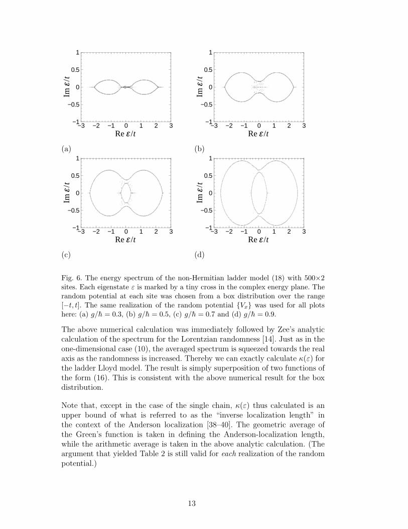
In Figure 6, I show a numerical result of the energy spectrum of a laddersystem,

H ≡ H1 + H2 −t

2

∑

x

(|x, 2〉 〈x, 1| + |x, 1〉 〈x, 2|) , (18)

where H1 and H2 is the non-Hermitian Anderson Hamiltonian for each leg ofthe ladder while the last term denotes hopping between the legs; “x, 1” and“x, 2” denote a site on the first and second leg, respectively. Alternatively wemay regard the labels 1 and 2 as an additional degree of freedom such as spinor flavor. On the basis of the argument in the previous subsection, we candeduce from the result in Fig. 6 that there are two minima of κ(ε) in theHermitian ladder system.

12

−1

−0.5

0

0.5

1

−3 −2 −1 0 1 2 3Re /tε

Im

/t ε

(a)

−1

−0.5

0

0.5

1

−3 −2 −1 0 1 2 3Re /tε

Im

/t ε

(b)

−1

−0.5

0

0.5

1

−3 −2 −1 0 1 2 3Re /tε

Im

/t ε

(c)

−1

−0.5

0

0.5

1

−3 −2 −1 0 1 2 3Re /tε

Im

/t ε

(d)

Fig. 6. The energy spectrum of the non-Hermitian ladder model (18) with 500×2sites. Each eigenstate ε is marked by a tiny cross in the complex energy plane. Therandom potential at each site was chosen from a box distribution over the range[−t, t]. The same realization of the random potential {Vx} was used for all plotshere: (a) g/h = 0.3, (b) g/h = 0.5, (c) g/h = 0.7 and (d) g/h = 0.9.

The above numerical calculation was immediately followed by Zee’s analyticcalculation of the spectrum for the Lorentzian randomness [14]. Just as in theone-dimensional case (10), the averaged spectrum is squeezed towards the realaxis as the randomness is increased. Thereby we can exactly calculate κ(ε) forthe ladder Lloyd model. The result is simply superposition of two functions ofthe form (16). This is consistent with the above numerical result for the boxdistribution.

Note that, except in the case of the single chain, κ(ε) thus calculated is anupper bound of what is referred to as the “inverse localization length” inthe context of the Anderson localization [38–40]. The geometric average ofthe Green’s function is taken in defining the Anderson-localization length,while the arithmetic average is taken in the above analytic calculation. (Theargument that yielded Table 2 is still valid for each realization of the randompotential.)

13

3.5 Energy spectrum in two dimension

Finite-size calculations of the energy spectrum of the non-Hermite Hamilto-nian (2) for d = 2 [1,2] appeared to suggest the following three regions ofthe non-Hermitian field ~g. First, it is widely accepted for ~g = ~0 that all eigen-states of two-dimensional random systems are localized with finite localizationlengths. Hence, by using the imaginary gauge transformation again, we canconclude that there is a finite region of small ~g where all states remain lo-calized. This is consistent with the finite-size data [1,2]. As ~g is increased,delocalized states with complex eigenvalues appear as in the one-dimensionalcase. For intermediate values of ~g, however, the energy spectrum shows muchmore complicated structure than in the one-dimensional case; see Ref. [2] fordetails. For larger ~g, the spectrum becomes similar to the one of the systemwithout impurities, as was the case in d = 1.

Nelson and Shnerb [11] suggested that the third region of ~g disappears in thethermodynamic limit. For a very large ~g, or a very large transverse magneticfield ~H⊥, the flux line lies nearly sideways in the superconductor. When weproject the flux line and the columnar defects onto a two-dimensional planefrom above, the problem is approximately reduced to a string lying on a planewith point impurities. Nelson and Shnerb analyzed this reduced problem interms of Burger’s equation with noise [41] (or the Kardar-Parisi-Zhang equa-tion [42]) and predicted a fractal geometry of the flux-line configuration. Thisfractality may cause the complicated energy spectrum observed in the sec-ond region of ~g. The fractal geometry does not emerge until the system sizebecomes larger than a certain crossover length, which can explain the appear-ance of the third region of ~g in the finite-size data [1,2]. The above theoreticalprediction is consistent with numerical results in Ref. [32], although the numer-ical estimate of the exponent characterizing the fractal geometry is somewhatdifferent from the theoretical value predicted by Nelson and Shnerb [11].

Note, however, that a different conclusion may be suggested by Zee’s ana-lytic calculation of the two-dimensional spectrum for the Lorentzian randompotential [14]. In the case of the Lorentzian random distribution, just as inone dimension, the averaged spectrum is squeezed towards the real axis asthe randomness is increased. In the process, the spectrum keeps the regularstructure of the spectrum of the non-random system.

4 Transverse Meissner effect

One of the interesting issues in the context of the flux-line depinning is how thetransverse Meissner effect breaks down as the depinning point is approached

14

from the side of the pinning phase. As is shown schematically in Fig. 2, thepinning breaks first near the surface. This is also observed in numerical re-sults [2]. Thus we can define a penetration depth τ ∗ for the transverse Meissnereffect as the typical thickness of the sub-surface region where the flux line isdeflected from the pinning center. (Note that τ ∗ is different from the pene-tration depth of the underlying superconductivity.) The penetration depth τ ∗

diverges with a certain exponent, as we increase ~H⊥, or ~g. This divergenceleads to the breakdown of the bulk pinning. The conclusion of Refs. [1,2] is

τ ∗ ∼ (H⊥c −H⊥)−d, (19)

where H⊥c is the depinning field. Note that the dimensionality of the super-conductor is d+ 1.

Since we regard the flux line as the world line of a quantum particle in theframework of the non-Hermitian quantum mechanics, the deflection of the fluxline is interpreted as hopping of the quantum particle from a strong impurity(the localization center) to weaker impurities. Near the delocalization pointgc(∝ H⊥c), Mott’s argument of variable-range hopping [43] is readily appli-cable even to the non-Hermitian case. Minimizing a hopping matrix elementnear the surface leads to Eq. (19).

5 Summary

A class of random non-Hermitian quantum systems has been found to berelevant to various physical systems and to show intriguing properties. In par-ticular, the delocalization phenomenon of the random non-Hermitian systemis equivalent to the depinning of a flux line in type-II superconductors. Wecan investigate the delocalization just by observing the energy spectrum ofthe non-Hermite Hamiltonian. Various depinning phenomena may be under-stood in a similar way. Interesting future problems include many-band non-Hermitian Anderson models, detection of the fractality in the spectrum ofthe two-dimensional system, and generalization of the theory to the case ofinteracting systems.

Acknowledgments

The author expresses his sincere gratitude to Prof. D.R. Nelson for collabo-ration and continuous encouragement. He is also grateful to Prof. A. Zee forvaluable and stimulating discussions.

15

A Path-integral mapping

I here show derivation of Eq. (4) from Eq. (3). There are various ways of for-mulating the path-integral mapping. The following is based on the formulationin Ref. [28], which employs the Trotter decomposition [15]:

e−LτH/h = limn→∞

(

e−V∆τ/h e−K∆τ/h)n. (A.1)

Here K and V denote the kinetic and potential terms of the Hamiltonian (1),respectively, and ∆τ ≡ Lτ/n.

The matrix element (3) is transformed as follows:

Z = limn→∞

⟨

ψf∣

∣

∣

(

e−V∆τ/h e−K∆τ/h)n ∣∣

∣ ψi⟩

= limn→∞

∫ n∏

k=0

d~xk

∫ n∏

k=1

d~pk

⟨

ψf∣

∣

∣ ~xn

⟩

×n∏

k=1

{

exp[

−∆τ

hV (~xk)

]

⟨

~xk

∣

∣

∣ ~pk

⟩

exp[

−∆τ

2mh(~pk + i~g)2

]

⟨

~pk

∣

∣

∣ ~xk−1

⟩

}

×⟨

~x0

∣

∣

∣ ψi⟩

. (A.2)

The plane wave is given by

⟨

~xk

∣

∣

∣ ~pk

⟩

=1

(2πh)d/2exp

[

i

h~pk · ~xk

]

(A.3)

Hence the integral over each ~pk in Eq. (A.2) is a Gaussian integral,

1

(2πh)d

∫

d~pk exp[

−∆τ

2mh(~pk + i~g)2 +

i

h~pk · ∆~xk

]

=(

m

2πh∆τ

)d/2

exp[

1

h~g · ∆~xk −

m

2h∆τ(∆~xk)

2]

, (A.4)

where ∆~xk ≡ ~xk − ~xk−1. Thus Eq. (A.2) is reduced to

Z = limn→∞

(

m

2πh∆τ

)nd/2 ∫(

n∏

k=0

d~xk

)

ψf(~xn)∗ψi(~x0)

× exp

−∆τ

h

n∑

k=1

m

2

(

∆~xk

∆τ

)2

− ~g ·∆~xk

∆τ+ V (~xk)

=∫

D~xψf(~x(Lτ ))∗ψi(~x(0))

16

× exp

−1

h

Lτ∫

0

dτ

m

2

(

d~x(τ)

dτ

)2

−~g ·d~x(τ)

dτ+ V(~x(τ))

. (A.5)

By assuming the free boundary conditions ψi(~x) = ψf(~x) = const., we arriveat Eq. (4) with Eq. (5).

References

[1] N. Hatano and D. R. Nelson, Phys. Rev. Lett. 77 (1996) 570.

[2] N. Hatano and D. R. Nelson, Phys. Rev. B 56 (1997) 8651.

[3] N. Shnerb, Phys. Rev. B 55 (1997) R3382.

[4] K.B. Efetov, Phys. Rev. Lett. 79 (1997) 491.

[5] J. Feinberg and A. Zee, Nucl. Phys. B 504 (1997) 579.

[6] R.A. Janik, M.A. Nowak, G. Papp and I. Zahed, cond-mat/9705098.

[7] P.W. Brouwer, P.G. Silvestov and C.W.J. Beenakker, Phys. Rev. B 56 (1997)R4333.

[8] J. Feinberg and A. Zee, Phys. Rev. E, to be published (cond-mat/9706218).

[9] I.Ya. Goldsheid and B.A. Khoruzhenko, cond-mat/9707230.

[10] E. Brezin and A. Zee, Nucl. Phys. B, to be published (cond-mat/9708029).

[11] D.R. Nelson and N. Shnerb, cond-mat/9708071.

[12] J. Feinberg and A. Zee, cond-mat/9710040.

[13] R.A. Janik, M.A. Nowak, G. Papp and I. Zahed, hep-ph/9710103.

[14] A. Zee, in the same proceedings.

[15] M. Suzuki, Prog. Theor. Phys. 56 (1976) 1454.

[16] B.M. McCoy and T.T. Wu, Il Nuovo Cimento 56B (1968) 311; see also E.H.Lieb and F.Y. Wu, in: Phase Transitions and Critical Phenomena Vol. 1, C.Domb and M.S. Green, eds. (Academic Press, London, 1972) p. 331.

[17] J. Miller and J. Wang, Phys. Rev. Lett. 76 (1996) 1461.

[18] J.T. Chalker and Z.J. Wang, Phys. Rev. Lett. 79 (1997) 1797.

[19] Ya.V. Fyodorov and H.-Ju. Sommers, Pis’ma Zh. Eksp. Teor. Fiz. 63 (1996)970 [JETP Lett. 63 (1996) 1026].

[20] Ya.V. Fyodorov and H.-Ju. Sommers, J. Math. Phys. 38 (1997) 1918.

17

[21] Ya.V. Fyodorov, B.A. Khoruzhenko and H.-Ju. Sommers, Phys. Lett. A 226(1997) 46.

[22] Ya.V. Fyodorov, B.A. Khoruzhenko and H.-Ju. Sommers, Phys. Rev. Lett. 79(1997) 557.

[23] R.A. Janik, M.A. Nowak, G. Papp, J. Wambach and I. Zahed, Phys. Rev. E 55(1997) 4100.

[24] R.A. Janik, M.A. Nowak, G. Papp and I. Zahed, Nucl. Phys. B 501 (1997) 603.

[25] R.A. Janik, M.A. Nowak, G. Papp and I. Zahed, hep-ph/9708418.

[26] J. Feinberg and A. Zee, Nucl. Phys. B 501 (1997) 643.

[27] R.P. Feynman and A.R. Hibbs, Quantum mechanics and path integrals

(McGraw-Hill, New York, 1965).

[28] L.S. Schulman, Techniques and applications of path integration (John Wiley &Sons, New York, 1981) Sections 1 and 4.

[29] D.R. Nelson and V. Vinokur, Phys. Rev. B 48 (1993) 13060.

[30] L. Civale, A.D. Marwick, T.K. Worthington, M.A. Kirk, J.R. Thompson, L.Krusin-Elbaum, Y. Sun, J.R. Clem, and F. Holtzberg, Phys. Rev. Lett. 67(1991) 648.

[31] R.C. Budhani, M. Suenaga, and S.H. Liou, Phys. Rev. Lett. 69 (1992) 3816.

[32] L.-W. Chen, L. Balents, M.P.A. Fisher and M.C. Marchetti, Phys. Rev. B 54(1996) 12798.

[33] P. Le Doussal, unpublished. See also Sec. IV D of Ref. [29].

[34] P. Lloyd, J. Phys. C: Solid State Phys. 2 (1969) 1717.

[35] T. Hirota and K. Ishii, Prog. Theor. Phys. 45 (1971) 1713.

[36] K. Ishii, Prog. Theor. Phys. Supple. 53 (1973) 77.

[37] D.J. Thouless, J. Phys. C: Solid State Phys. 5 (1972) 77.

[38] R. Johnston and H. Kunz, J. Phys. C: Solid State Phys. 16 (1983) 4565.

[39] D.J. Thouless, J. Phys. C: Solid State Phys. 16 (1983) L929.

[40] D.E. Rodrigues, H.M. Pastawski adn J.F. Weisz, Phys. Rev. B 34 (1986) 8545.

[41] D. Forster, D.R. Nelson and M. Stephen, Phys. Rev. A 16 (1977) 732.

[42] M. Kardar, G. Parisi and Y.C. Zhang, Phys. Rev. Lett. 56 (1986) 889.

[43] For example, B.I. Shklovskii and A.L. Efros, Electronic Properties of DopedSemiconductors (Springer-Verlag, New York, 1984).

18