1 Fundamental Properties of Superconductors - Wiley-VCH
64
11 1 Fundamental Properties of Superconductors e vanishing of the electrical resistance, the observation of ideal diamagnetism, or the appearance of quantized magnetic flux lines represent characteristic prop- erties of superconductors that we will discuss in detail in this chapter. We will see that all of these properties can be understood, if we associate the superconducting state with a macroscopic coherent matter wave. In this chapter, we will also learn about experiments convincingly demonstrating this wave property. First we turn to the feature providing the name “superconductivity.” 1.1 The Vanishing of the Electrical Resistance e initial observation of the superconductivity of mercury raised a fundamen- tal question about the magnitude of the decrease in resistance on entering the superconducting state. Is it correct to talk about the vanishing of the electrical resistance? During the first investigations of superconductivity, a standard method for mea- suring electrical resistance was used. e electrical voltage across a sample car- rying an electric current was measured. Here, one could only determine that the resistance dropped by more than a factor of a thousand when the superconducting state was entered. One could only talk about the vanishing of the resistance in that the resistance fell below the sensitivity limit of the equipment and, hence, could no longer be detected. Here, we must realize that in principle it is impossible to prove experimentally that the resistance has exactly zero value. Instead, experimentally, we can only find an upper limit of the resistance of a superconductor. Of course, to understand such a phenomenon, it is highly important to test with the most sensitive methods to see whether a finite residual resistance can also be found in the superconducting state. So we are dealing with the problem of measur- ing extremely small values of the resistance. Already in 1914 Kamerlingh-Onnes used by far the best technique for this purpose. He detected the decay of an electric current flowing in a closed superconducting ring. If an electrical resistance exists, the stored energy of such a current is transformed gradually into joule heat. Hence, we need to only monitor such a current. If it decays as a function of time, we can be certain that a resistance still exists. If such a decay is observed, one can deduce Superconductivity: An Introduction, ird Edition. Reinhold Kleiner and Werner Buckel. © 2016 Wiley-VCH Verlag GmbH & Co. KGaA. Published 2016 by Wiley-VCH Verlag GmbH & Co. KGaA.
-
Upload
khangminh22 -
Category
Documents
-
view
3 -
download
0
Transcript of 1 Fundamental Properties of Superconductors - Wiley-VCH

11
1Fundamental Properties of Superconductors
The vanishing of the electrical resistance, the observation of ideal diamagnetism,or the appearance of quantized magnetic flux lines represent characteristic prop-erties of superconductors that we will discuss in detail in this chapter. We will seethat all of these properties can be understood, if we associate the superconductingstate with a macroscopic coherent matter wave. In this chapter, we will also learnabout experiments convincingly demonstrating this wave property. First we turnto the feature providing the name “superconductivity.”
1.1The Vanishing of the Electrical Resistance
The initial observation of the superconductivity of mercury raised a fundamen-tal question about the magnitude of the decrease in resistance on entering thesuperconducting state. Is it correct to talk about the vanishing of the electricalresistance?During the first investigations of superconductivity, a standardmethod formea-
suring electrical resistance was used. The electrical voltage across a sample car-rying an electric current was measured. Here, one could only determine that theresistance dropped bymore than a factor of a thousandwhen the superconductingstate was entered. One could only talk about the vanishing of the resistance in thatthe resistance fell below the sensitivity limit of the equipment and, hence, could nolonger be detected. Here, wemust realize that in principle it is impossible to proveexperimentally that the resistance has exactly zero value. Instead, experimentally,we can only find an upper limit of the resistance of a superconductor.Of course, to understand such a phenomenon, it is highly important to test with
the most sensitive methods to see whether a finite residual resistance can also befound in the superconducting state. Sowe are dealingwith the problem ofmeasur-ing extremely small values of the resistance. Already in 1914 Kamerlingh-Onnesused by far the best technique for this purpose.He detected the decay of an electriccurrent flowing in a closed superconducting ring. If an electrical resistance exists,the stored energy of such a current is transformed gradually into joule heat. Hence,we need to only monitor such a current. If it decays as a function of time, we canbe certain that a resistance still exists. If such a decay is observed, one can deduce
Superconductivity: An Introduction, Third Edition. Reinhold Kleiner and Werner Buckel.© 2016 Wiley-VCH Verlag GmbH & Co. KGaA. Published 2016 by Wiley-VCH Verlag GmbH & Co. KGaA.

12 1 Fundamental Properties of Superconductors
First cool down – than take magnet away
N
T > Tc
Normal conducting ring Superconducting ringwith persistent current Is
T < Tc
BB
Is
Figure 1.1 The generation of a permanent current in a superconducting ring.
an upper limit of the resistance from the temporal change and from the geometryof the superconducting circuit.This method is more sensitive by many orders of magnitude than the usual
current–voltage measurement. It is shown schematically in Figure 1.1. A ringmade from a superconducting material, say, from lead, is held in the normal stateabove the transition temperature Tc. A magnetic rod serves for applying a mag-netic field penetrating the ring opening. Nowwe cool the ring below the transitiontemperature Tc at which it becomes superconducting. The magnetic field1) pene-trating the opening practically remains unchanged. Subsequently we remove themagnet. This induces an electric current in the superconducting ring, since eachchange of the magnetic flux Φ through the ring causes an electrical voltage alongthe ring. This induced voltage then generates the current.If the resistance had exactly zero value, this current would flow without any
change as a “permanent current” as long as the lead ring remained superconduct-ing. However, if there exists a finite resistance R, the current would decrease withtime, following an exponential decay law. We have
I(t) = I0e−(R∕L)t (1.1)
Here, I0 denotes the current at some time that we take as time zero; I(t) is the cur-rent at time t; R is the resistance; and L is the self-induction coefficient, dependingonly upon the geometry of the ring.2)
1) Throughout we will use the quantity B to describe the magnetic field and, for simplicity, refer toit as “magnetic field” instead of “magnetic flux density.” Since the magnetic fields of interest (alsothose within the superconductor) are generated by macroscopic currents only, we do not have todistinguish between the magnetic fieldH and the magnetic flux density B, except for a few cases.
2) The self-induction coefficient L can bedefined as the proportionality factor betweenthe induction voltage along a conductor andthe temporal change of the current passingthrough the conductor: Uind = −L(dI∕dt).The energy stored within a ring carrying apermanent current is given by (1/2)LI2. The
temporal change of this energy is exactlyequal to the joule heating power RI2dissipated within the resistance. Hence, wehave −(d∕dt)((1∕2)LI2) = RI2. One obtainsthe differential equation −(dI∕dt) = (R∕L)I,the solution of which is Eq. (1.1).

1.1 The Vanishing of the Electrical Resistance 13
For an estimate, we assume that we are dealing with a ring of 5 cm diametermade fromawirewith a thickness of 1mm.The self-induction coefficientL of sucha ring is about 1.3× 10⁻⁷ H. If the permanent current in such a ring decreases byless than 1% within an hour, we can conclude that the resistance must be smallerthan 4× 10⁻¹³ Ω.3) This means that in the superconducting state the resistance haschanged by more than 8 orders of magnitude.During such experiments the magnitude of the permanent current must be
monitored. Initially [1] this was simply accomplished by means of a magneticneedle, its deflection in the magnetic field of the permanent current beingobserved. A more sensitive setup was used by Kamerlingh-Onnes and somewhatlater by Tuyn [2]. It is shown schematically in Figure 1.2. In both superconductingrings 1 and 2, a permanent current is generated by an induction process. Becauseof this current both rings are kept in a parallel position. If one of the rings (herethe inner one) is suspended from a torsion thread and is slightly turned awayfrom the parallel position, the torsion thread experiences a force originatingfrom the permanent current. As a result, an equilibrium position is establishedin which the angular moments of the permanent current and of the torsionthread balance each other. This equilibrium position can be observed verysensitively using a light beam. Any decay of the permanent current within therings would be indicated by the light beam as a change in its equilibrium position.During all such experiments, no change of the permanent current has ever beenobserved.A nice demonstration of superconducting permanent currents is shown in
Figure 1.3. A small permanent magnet that is lowered toward a superconductinglead bowl generates induction currents according to Lenz’s rule, leading toa repulsive force acting on the magnet. The induction currents support themagnet at an equilibrium height. This arrangement is referred to as a levitatedmagnet. The magnet is supported as long as the permanent currents are flowingwithin the lead bowl, that is, as long as the lead remains superconducting.For high-temperature superconductors such as YBa2Cu3O7, the levitation caneasily be performed using liquid nitrogen in regular air. Furthermore, it can alsoserve for levitating freely real heavyweights such as the Sumo wrestler shown inFigure 1.4.The most sensitive arrangements for determining an upper limit of the resis-
tance in the superconducting state are based on geometries having an extremelysmall self-induction coefficient L, in addition to an increase in the observationtime. In this way, the upper limit can be lowered further. A further increase in thesensitivity is accomplished by themodern superconductingmagnetic field sensors(see Section 7.6.4). Today, we know that the jump in resistance during entry intothe superconducting state amounts to at least 14 orders of magnitude [3]. Hence,in the superconducting state, a metal can have a specific electrical resistance that
3) For a circular ring of radius r made from a wire of thickness 2d also with circular cross-section(r ≫ d), we have L=𝜇0r [ln(8r/d)− 1.75] with 𝜇0 = 4𝜋 × 10−7 V s/Am. It follows that
R ≤ − ln 0.99 × 1.3 × 10−7
3.6 × 10³VsAm
≅ 3.6 × 10⁻¹³ Ω

14 1 Fundamental Properties of Superconductors
Torque wire
Mirror
Light pointer
Ring 1
Ring 2
(a)
(b)
Figure 1.2 Arrangement for the observation of a permanent current. (a) side view, (b) topview. (After [2].) Ring 1 is attached to the cryostat.
(a) (b)
Figure 1.3 The “levitated magnet” for demonstrating the permanent currents that are gen-erated in superconducting lead by induction during the lowering of the magnet. (a) Startingposition. (b) Equilibrium position.

1.1 The Vanishing of the Electrical Resistance 15
Figure 1.4 Application of free levitationby means of the permanent currents in asuperconductor. The Sumo wrestler (includ-ing the plate at the bottom) weighs 202 kg.
The superconductor is YBa2Cu3O7. (Photo-graph kindly supplied by the InternationalSuperconductivity Research Center (ISTEC)and Nihon-SUMO Kyokai, Japan, 1997.)
is at most about 17 orders of magnitude smaller than the specific resistance ofcopper, one of our best metallic conductors, at 300K. Since hardly anyone has aclear idea about “17 orders of magnitude,” we also present another comparison:the difference in resistance of a metal between the superconducting and normalstates is at least as large as that between copper and a standard electrical insulator.Following this discussion, it appears justified at first to assume that in the
superconducting state the electrical resistance actually vanishes. However, wemust point out that this statement is valid only under specific conditions. Sothe resistance can become finite even in the case of small transport currents, ifmagnetic flux lines exist within the superconductor. Furthermore, alternatingcurrents experience a resistance that is different from zero. We return to thissubject in more detail in subsequent chapters.This totally unexpected behavior of the electric current, flowing without resis-
tance through a metal and at the time contradicting all well-supported concepts,becomes evenmore surprising if we lookmore closely at charge transport throughametal. In this way, we can also appreciatemore strongly the problem confrontingus in terms of an understanding of superconductivity.

16 1 Fundamental Properties of Superconductors
We know that electric charge transport in metals takes place through the elec-trons. The concept that, in a metal, a definite number of electrons per atom (forinstance, in the alkalis, one electron, the valence electron) exist freely, rather likea gas, was developed at an early time (by Paul Drude in 1900, and Hendrik AntonLorentz in 1905). These “free” electrons also mediate the binding of the atomsin metallic crystals. In an applied electric field the free electrons are accelerated.After a specific time, the mean collision time 𝜏 , they collide with atoms andlose the energy they have taken up from the electric field. Subsequently, theyare accelerated again. The existence of the free charge carriers, interacting withthe lattice of the metallic crystal, results in the high electrical conductivity ofmetals.Also the increase in the resistance (decrease in the conductivity) with increas-
ing temperature can be understood immediately. With increasing temperature,the uncorrelated thermal motion of the atoms in a metal (each atom is vibrat-ing with a characteristic amplitude about its equilibrium position) becomes morepronounced. Hence, the probability for collisions between the electrons and theatoms increases, that is, the time 𝜏 between two collisions becomes smaller. Sincethe conductivity is directly proportional to this time, in which the electrons arefreely accelerated because of the electric field, it decreases with increasing tem-perature and the resistance increases.This “free-electron model,” according to which electron energy can be deliv-
ered to the crystal lattice only due to the collisions with the atomic ions, providesa plausible understanding of electrical resistance. However, within this model, itappears totally inconceivable that, within a very small temperature interval at afinite temperature, these collisions with the atomic ions should abruptly becomeforbidden. Which mechanism(s) could have the effect that, in the superconduct-ing state, energy exchange between electrons and lattice is not allowed any more?This appears to be an extremely difficult question.Based on the classical theory of matter, another difficulty appeared with the
concept of the free-electron gas in a metal. According to the general rules ofclassical statistical thermodynamics, each degree of freedom4) of a system onaverage should contribute kBT/2 to the internal energy of the system. Here,kB = 1.38× 10⁻²³ W s/K is Boltzmann’s constant. This also means that the freeelectrons are expected to contribute the amount of energy 3kBT/2 per free elec-tron, characteristic for a monatomic gas. However, specific heat measurementsof metals have shown that the contribution of the electrons to the total energy ofmetals is about a thousand times smaller than expected from the classical laws.Here, one can see clearly that the classical treatment of the electrons in met-
als in terms of a gas of free electrons does not yield a satisfactory understand-ing. On the other hand, the discovery of energy quantization by Max Planck in1900 started a totally new understanding of physical processes, particularly on the
4) Each coordinate of a system that appears quadratically in the total energy represents a thermo-dynamic degree of freedom, for example, the velocity v for Ekin = (1/2)mv2, or the displacement xfrom the equilibrium position for a linear law for the force, Epot = (1/2)Dx2, where D is the forceconstant.

1.1 The Vanishing of the Electrical Resistance 17
atomic scale. The following decades then demonstrated the overall importance ofquantum theory and of the new concepts resulting from the discovery made byMax Planck. Also the discrepancy between the observed contribution of the freeelectrons to the internal energy of a metal and the amount expected from the clas-sical theory was resolved by Arnold Sommerfeld in 1928 bymeans of the quantumtheory.The quantum theory is based on the fundamental idea that each physical system
is described in terms of discrete states. A change of physical quantities such as theenergy can only take place by a transition of the system from one state to another.This restriction to discrete states becomes particularly clear for atomic objects. In1913, Niels Bohr proposed the first stable model of an atom, which could explaina large number of facts hitherto not understood. Bohr postulated the existence ofdiscrete stable states of atoms. If an atom in some way interacts with its environ-ment, say, by the gain or loss of energy (e.g., due to the absorption or emission oflight), then this is possible only within discrete steps in which the atom changesfrom one discrete state to another. If the amount of energy (or that of anotherquantity to be exchanged) required for such a transition is not available, the stateremains stable.In the final analysis, this relative stability of quantum mechanical states also
yields the key to the understanding of superconductivity. Aswe have seen, we needsomemechanism(s) forbidding the interaction between the electrons carrying thecurrent in a superconductor and the crystal lattice. If one assumes that the “su-perconducting” electrons occupy a quantum state, some stability of this state canbe understood. Already in about 1930, the concept became accepted that super-conductivity represents a typical quantum phenomenon. However, there was stilla long way to go for a complete understanding. One difficulty originated fromthe fact that quantum phenomena were expected for atomic systems, but not formacroscopic objects. In order to characterize this peculiarity of superconductiv-ity, one often referred to it as a macroscopic quantum phenomenon. Below we willunderstand this notation even better.Inmodern physics another aspect has also been developed, whichmust bemen-
tioned at this stage, since it is needed for a satisfactory understanding of somesuperconducting phenomena. We have learned that the particle picture and thewave picture represent complementary descriptions of one and the same physicalobject. Here, one can use the simple rule that propagation processes are suitablydescribed in terms of the wave picture and exchange processes during the inter-action with other systems in terms of the particle picture.We illustrate this important point with two examples. Light appears to us as
a wave because of many diffraction and interference effects. On the other hand,during the interaction with matter, say, in the photoelectric effect (knocking anelectron out of a crystal surface), we clearly notice the particle aspect. One findsthat independently of the light intensity the energy transferred to the electron onlydepends upon the light frequency. However, the latter is expected if light repre-sents a current of particles where all particles have an energy depending on thefrequency.

18 1 Fundamental Properties of Superconductors
For electrons, we are more used to the particle picture. Electrons can bedeflected by means of electric and magnetic fields, and they can be thermallyevaporated from metals (glowing cathode). All these are processes where theelectrons are described in terms of particles. However, Louis de Broglie proposedthe hypothesis that each moving particle also represents a wave, where thewavelength 𝜆 is equal to Planck’s constant h divided by the magnitude p of theparticle momentum, that is, 𝜆= h/p. The square of the wave amplitude at thelocation (x, y, z) then is a measure of the probability of finding the particle at thislocation.We see that the particle is spatially “smeared” over some distance. If we want to
favor a specific location of the particle within the wave picture, we must constructa wave with a pronounced maximum amplitude at this location. Such a wave isreferred to as a wave packet. The velocity with which the wave packet spatiallypropagates is equal to the particle velocity.Subsequently, this hypothesis was brilliantly confirmed. With electrons we can
observe diffraction and interference effects. Similar effects also exist for other par-ticles, say, for neutrons. The diffraction of electrons and neutrons has developedinto important techniques for structural analysis. In an electron microscope, wegenerate images bymeans of electron beams and achieve a spatial resolutionmuchhigher than that for visible light because of the much smaller wavelength of theelectrons.For the matter wave associated with the moving particle, there exists, like
for each wave process, a characteristic differential equation, the fundamentalSchrödinger equation. This deeper insight into the physics of electrons must alsobe applied to the description of the electrons in a metal. The electrons withina metal also represent waves. Using a few simplifying assumptions, from theSchrödinger equation we can calculate the discrete quantum states of these elec-tron waves in terms of a relation between the allowed energies E and the so-calledwave vector k. The magnitude of k is given by 2π/𝜆, and the spatial direction ofk is the propagation direction of the wave. For a completely free electron, thisrelation is very simple. We have in this case
E = ℏ2𝐤22m
(1.2)
where m is the electron mass and ℏ = h∕2π.However, within a metal the electrons are not completely free. First, they are
confined to the volume of the piece of metal, like in a box. Therefore, the allowedvalues of k are discrete, simply because the allowed electron waves must satisfyspecific boundary conditions at the walls of the box. For example, the amplitudeof the electron wave may have to vanish at the boundary.Second, within the metal the electrons experience the electrostatic forces orig-
inating from the positively charged atomic ions, in general arranged periodically.This means that the electrons exist within a periodic potential. Near the positivelycharged atomic ions, the potential energy of the electrons is lower than betweenthese ions. As a result of this periodic potential, in the relation between E and k,

1.1 The Vanishing of the Electrical Resistance 19
E
EF
k
Figure 1.5 Energy–momentum relation for an electron in a periodic potential. The relation(Eq. (1.2)) valid for free electrons is shown as the dashed parabolic line.
not all energies are allowed any more. Instead, there exist different energy rangesseparated from each other by ranges with forbidden energies. An example of suchan E–k dependence, modified because of a periodic potential, is shown schemat-ically in Figure 1.5.So nowwe are dealing with energy bands.The electronsmust be filled into these
bands. Here, we have to pay attention to another important principle formulatedbyWolfgang Pauli in 1924.This “Pauli principle” requires that in quantum physicseach discrete state can be occupied only by a single electron (or more generally bya single particle with a half-integer spin, a so-called “fermion”). Since the angularmomentum (spin) of the electrons represents another quantum number with twopossible values, according to the Pauli principle each of the discrete k-values canbe occupied by only two electrons. In order to accommodate all the electrons ofa metal, the states must be filled up to relatively high energies. The maximumenergy up to which the states are being filled is referred to as the Fermi energyEF. The density of states per energy interval and per unit volume is referred tosimply as the density of states N(E). In the simplest case, in momentum space thefilled states represent a sphere, the so-called Fermi sphere. However, in general,one finds more complex objects. In a metal the Fermi energy is located within anallowed energy band, that is, the band is only partly filled.5) In Figure 1.5, the Fermienergy is indicated for this case.The occupation of the states is determined by the distribution function for a
system of fermions, the Fermi function. This Fermi function takes into account
5) We have an electrical insulator if the accommodation of all the electrons only leads to completelyfilled bands. The electrons of a filled band cannot take up energy from the electric field, since nofree states are available.

20 1 Fundamental Properties of Superconductors
1
00 EF
Energy E
T>0
T=0F
erm
i fu
nctio
n
Figure 1.6 Fermi function. EF is a few electronvolts, whereas thermal smearing is only afew 10−3 eV. To indicate this, the abscissa is interrupted.
the Pauli principle and is given by
f = 1e(E−EF)∕kBT + 1
(1.3)
where kB is Boltzmann’s constant and EF is the Fermi energy. This Fermi func-tion is shown in Figure 1.6 for the case T = 0 (dashed line) and for the case T > 0(solid line). For finite temperatures, the Fermi function is slightly smeared out.This smearing is equal to about the average thermal energy of the fermions. Atroom temperature, it amounts to about 1∕40eV.6) At finite temperatures, the Fermienergy is the energy at which the distribution function has the value 1/2. In atypical metal, it amounts to about a few electronvolts.This has the important con-sequence that at normal temperatures the smearing of the Fermi edge is very small.Such an electron system is referred to as a degenerate electron gas.At this stage, we can also understand the very small contribution of the electrons
to the internal energy. According to the concepts we have discussed earlier, onlyvery few electrons, namely those within the energy smearing of the Fermi edge,can participate in the thermal energy exchange processes. All other electrons can-not be excited with thermal energies, since they do not find empty states that theycould occupy after their excitation.We have to become familiar with the concept of quantum states and their
occupation if we want to understand modern solid-state physics. This is alsonecessary for an understanding of superconductivity. In order to get used tothe many new ideas, we will briefly discuss the mechanism generating electricalresistance. The electrons are described in terms of waves propagating in alldirections through the crystal. An electric current results if slightly more wavespropagate in one direction than in the opposite direction. The electron wavesare scattered because of their interaction with the atomic ions. This scatteringcorresponds to collisions in the particle picture. What is new in the wave picture
6) eV (electronvolt) is the standard energy unit of elementary processes: 1 eV= 1.6× 10⁻¹⁹ W s.

1.2 Ideal Diamagnetism, Flux Lines, and Flux Quantization 21
is the fact that this scattering cannot take place for a strongly periodic crystallattice. The states of the electrons resulting as the solutions of the Schrödingerequation represent stable quantum states. Only a perturbation of the periodicpotential, caused by thermal vibrations of the atoms, by defects in the crystallattice, or by chemical impurities, can lead to a scattering of the electron waves,that is, to a change in the occupation of the quantum states. The scattering dueto the thermal vibrations yields a temperature-dependent component of theresistance, whereas that at crystal defects and chemical impurities yields theresidual resistance.After this brief and simplified excursion into the modern theoretical treatment
of electronic conduction, we return to our central problem, charge transport withzero resistance in the superconducting state. Also the new wave mechanical ideasdo not yet provide an easy access to the appearance of a permanent current. Wehave only changed the language. Now we must ask: Which mechanisms com-pletely eliminate any energy exchange with the crystal lattice by means of scat-tering at finite temperatures within a very narrow temperature interval? It turnsout that an additional new aspect must be taken into account, namely a particu-lar interaction between the electrons themselves. In our previous discussion wehave treated the quantum states of the individual electrons, and we have assumedthat these states do not change when they become occupied with electrons. How-ever, if an interaction exists between the electrons, this treatment is no longercorrect. Now we must ask instead: What are the states of the system of electronswith an interaction, that is, what collective states exist? Here, we encounter theunderstanding and also the difficulty of superconductivity. It is a typical collectivequantum phenomenon characterized by the formation of a coherent matter wave,propagating through the superconductor without any friction.
1.2Ideal Diamagnetism, Flux Lines, and Flux Quantization
It has been known for a long time that the characteristic property of the super-conducting state is that it shows no measurable resistance for direct current. Ifa magnetic field is applied to such an ideal conductor, permanent currents aregenerated by induction, which screen the magnetic field from the interior of thesample. In Section 1.1 we have seen this principle already for the levitatedmagnet.What happens if a magnetic fieldBa is applied to a normal conductor and if sub-
sequently, by cooling below the transition temperatureTc, ideal superconductivityis reached? At first, in the normal state, on application of the magnetic field, eddycurrents flow because of induction. However, as soon as themagnetic field reachesits final value and no longer changes with time, these currents decay according toEq. (1.1), and finally the magnetic fields within and outside the superconductorbecome equal.If now the ideal conductor is cooled below Tc, this magnetic state simply
remains, since further induction currents are generated only during changes of

22 1 Fundamental Properties of Superconductors
the field. Exactly this is expected, if the magnetic field is turned off below Tc. Inthe interior of the ideal conductor, the magnetic field remains conserved.Hence, depending on theway inwhich the final state, namely temperature below
Tc and appliedmagnetic fieldBa, has been reached, within the interior of the idealconductor we have completely different magnetic fields.An experiment by Kamerlingh-Onnes from 1924 appeared to confirm exactly
this complicated behavior of a superconductor. Kamerlingh-Onnes [4] cooled ahollow sphere made of lead below the transition temperature in the presence ofan applied magnetic field and subsequently turned off the external magnetic field.Then he observed permanent currents and a magnetic moment of the sphere, asexpected for the case R= 0.Accordingly, a material with the property R= 0, for the same external variables
T and Ba, could be transferred into completely different states, depending onthe previous history. Therefore, for the same given thermodynamic variables, wewould not have just one well-defined superconducting phase, but, instead, a con-tinuous manifold of superconducting phases with arbitrary shielding currents,depending on the previous history. However, the existence of a manifold of super-conducting phases appeared so unlikely that, before 1933, one referred to only asingle superconducting phase [5] even without experimental verification.However, a superconductor behaves quite differently from an ideal electrical
conductor. Again, we imagine that a sample is cooled below Tc in the presence ofan appliedmagnetic field. If thismagnetic field is very small, one finds that the fieldis completely expelled from the interior of the superconductor except for a verythin layer at the sample surface. In this way, one obtains an ideal diamagnetic state,independent of the temporal sequence inwhich themagnetic fieldwas applied andthe sample was cooled.This ideal diamagnetismwas discovered in 1933 byMeissner andOchsenfeld for
rods made of lead or tin [6]. This expulsion effect, similar to the property R= 0,can be nicely demonstrated using the “levitated magnet.”7) In order to show theproperty R= 0, in Figure 1.3 we have lowered the permanent magnet toward thesuperconducting lead bowl, in this way generating permanent currents by induc-tion. To demonstrate the Meissner–Ochsenfeld effect, we place the permanentmagnet into the lead bowl at T >Tc (Figure 1.7a) and then cool down further.Thefield expulsion appears at the superconducting transition: the magnet is repelledfrom the diamagnetic superconductor, and it is raised up to the equilibrium height(Figure 1.7b). In the limit of ideal magnetic field expulsion, the same levitationheight is reached as in Figure 1.3.What went wrong during the original experiment of Kamerlingh-Onnes? He
used a hollow sphere in order to consume a smaller amount of liquid helium forcooling. The observations for this sample were correct. However, he had over-looked the fact that during cooling of a hollow sphere a closed ring-shaped super-conducting object can be formed, which keeps the magnetic flux penetrating its
7) Also non-superconducting, but diamagnetic objects, such as nuts or frogs, can levitate above mag-nets. However, one needs very large field gradients [7].

1.2 Ideal Diamagnetism, Flux Lines, and Flux Quantization 23
(a) (b)
Figure 1.7 “Levitated magnet” for demonstrating the Meissner–Ochsenfeld effect in thepresence of an applied magnetic field. (a) Starting position at T > Tc. (b) Equilibrium posi-tion at T < Tc.
open area constant. Hence, a hollow sphere can act like a superconducting ring(Figure 1.1), leading to the observed result.Above, we had assumed that the magnetic field applied to the superconductor
would be “small.” Indeed, one finds that ideal diamagnetism only exists withina finite range of magnetic fields and temperatures, which, furthermore, alsodepends on the sample geometry.Next, we consider a long, rod-shaped sample where themagnetic field is applied
parallel to the axis. For other shapes, the magnetic field can often be distorted. Foran ideal diamagnetic sphere, at the “equator” the magnetic field is 1.5 times largerthan the externally applied field. In Section 4.6.4, we will discuss these geometriceffects in more detail.One finds that there exist two different types of superconductors:
• The first type, referred to as type-I superconductors or superconductors of thefirst kind, expels the magnetic field up to a maximum value Bc, the critical field.For larger fields, superconductivity breaks down, and the sample assumes thenormal conducting state. Here, the critical field depends on the temperature andreaches zero at the transition temperature Tc. Mercury and lead are examplesof a type-I superconductor.
• The second type, referred to as type-II superconductors or superconductors ofthe second kind, shows ideal diamagnetism for magnetic fields smaller than the“lower critical magnetic field” Bc1. Superconductivity completely vanishes formagnetic fields larger than the “upper critical magnetic field” Bc2, which oftenis much larger than Bc1. Both critical fields reach zero at Tc. This behavior isfound in many alloys and also in the high-temperature superconductors. In thelatter, Bc2 can reach even values larger than 100T.
What happens in type-II superconductors in the “Shubnikov phase” betweenBc1 and Bc2? In this regime, the magnetic field only partly penetrates into the sam-ple. Now shielding currents flow within the superconductor and concentrate themagnetic field lines, such that a system of flux lines, also referred to as Abrikosov

24 1 Fundamental Properties of Superconductors
Ba
Figure 1.8 Schematic diagram of the Shubnikov phase. The magnetic field and the super-currents are shown only for two flux lines.
vortices, is generated. For the prediction of quantized flux lines, A. A. Abrikosovreceived the Nobel Prize in physics in 2003. In an ideal homogeneous supercon-ductor in general, these vortices arrange themselves in the form of a triangularlattice. In Figure 1.8 we show schematically this structure of the Shubnikov phase.The superconductor is penetrated by magnetic flux lines, each of which carriesa magnetic flux quantum and is located at the corners of equilateral triangles.Each flux line consists of a system of circulating currents, which in Figure 1.8 areindicated for two flux lines. These currents together with the external magneticfield generate the magnetic flux within the flux line and reduce the magnetic fieldbetween the flux lines. Hence, one also talks about flux vortices. With increasingexternal field Ba, the distance between the flux lines becomes smaller.The first experimental proof of a periodic structure of the magnetic field in the
Shubnikov phase was given in 1964 by a group at the Nuclear Research Cen-ter in Saclay using neutron diffraction [8]. However, they could only observe abasic period of the structure. Beautiful neutron diffraction experiments with thismagnetic structure were performed by a group at the Nuclear Research Center,Jülich [9]. Real images of the Shubnikov phase were generated by Essmann andTräuble [10] using an ingenious decoration technique. In Figure 1.9, we show alead–indium alloy as an example. These images of the magnetic flux structurewere obtained as follows: Above the superconducting sample, iron atoms are evap-orated from a hot wire. During their diffusion through the helium gas in the cryo-stat, the iron atoms coagulate to form iron colloids.These colloids have a diameterof less than 50 nm, and they slowly approach the surface of the superconductor. Atthis surface, the flux lines of the Shubnikov phase exit from the superconductor.In Figure 1.8, this is shown for two flux lines.The ferromagnetic iron colloid is col-lected at the locations where the flux lines exit from the surface, since here they

1.2 Ideal Diamagnetism, Flux Lines, and Flux Quantization 25
Figure 1.9 Image of the vortex latticeobtained with an electron microscope follow-ing the decoration with iron colloid. Frozen-in flux after the magnetic field has beenreduced to zero. Material: Pb +6.3 at% In;
temperature: 1.2 K; sample shape: cylinder,60mm long, 4mm diameter; and magneticfield Ba parallel to the axis. Magnification:8300×. (Reproduced by courtesy of Dr Ess-mann.)
find the largest magnetic field gradients. In this way, the flux lines can be dec-orated. Subsequently, the structure can be observed in an electron microscope.The image shown in Figure 1.9 was obtained in this way. Such experiments con-vincingly confirmed the vortex structure predicted theoretically by Abrikosov.The question remains whether the decorated locations at the surface indeed
correspond to the ends of the flux lines carrying only a single flux quantum. Inorder to answer this question, we just have to count the number of flux lines andalso have to determine the total flux, say, by means of an induction experiment.Then we find the value of the magnetic flux of a flux line by dividing the totalfluxΦtot through the sample by the number of flux lines. Such evaluations exactlyconfirmed that in highly homogeneous type-II superconductors, each flux linecontains a single flux quantum Φ0 = 2.07× 10⁻¹⁵ Tm2.Today, we know different methods for imaging magnetic flux lines. Often, the
methods supplement each other and provide valuable information about super-conductivity. Therefore, we will discuss some of them in more detail.Neutron diffraction and decoration still represent important techniques.
Figure 1.10a shows a diffraction pattern observed at the Institute Laue-Langevinin Grenoble by means of neutron diffraction at the vortex lattice in niobium. Thetriangular structure of the vortex lattice can clearly be seen from the diffractionpattern.Magneto-optics represents another method for spatially imaging magnetic
structures. Here, one utilizes the Faraday effect. If linearly polarized light passesthrough a thin layer of a “Faraday-active” material such as a ferrimagnetic garnetfilm, the plane of polarization of the light will be rotated due to a magnetic fieldwithin the garnet film. A transparent substrate, covered with a thin ferrimagneticgarnet film, is placed on top of a superconducting sample and is irradiated withpolarized and well-focused light. The light is reflected at the superconductor,passes through the ferrimagnetic garnet film again, and is then focused into aCCD camera. The magnetic field from the vortices in the superconductor pene-trates into the ferrimagnetic garnet film and there causes a rotation of the planeof polarization of the light. An analyzer located in front of the CCD camera onlytransmits light whose polarization is rotated away from the original direction.

26 1 Fundamental Properties of Superconductors
(a) (b)
(d)
(e) (f)
(c)
Vacuum
0.1 inform 0.00 mV
1000 Gauss
0.01 1.75
Pb2 μm
10 μm
40 μm
Figure 1.10 Methods for the imaging offlux lines. (a) Neutron diffraction pattern ofthe vortex lattice in niobium (Figure kindlyprovided by Institute Max von Laue-PaulLangevin, Grenoble; Authors: E. M. For-gan (Univ. Birmingham), S. L. Lee (Univ. St.Andrews), D. McK.Paul (Univ. Warwick), H.A. Mook (Oak Ridge) and R. Cubitt (ILL).). (b)Magneto-optical image of vortices in NbSe2
[11]. (c) Lorentz microscopy of niobium(Figure kindly provided by A. Tonomura, Fa.Hitachi Ltd.). (d) Electron holography of Pb[12]. (e) Low-temperature scanning electronmicroscopy of YBa2Cu3O7 [13]. (f ) Scanningtunneling microscopy of NbSe2 (Figure kindlyprovided by Fa. Lucent Technologies Inc./Belllabs).
In this way, the vortices appear as bright dots, as shown in Figure 1.10b for thecompound NbSe2 [11].8) This method yields a spatial resolution of more than1 μm. Presently, one can take about 10 images/s, also allowing the observationof dynamic processes. Unfortunately, at this time, the method is restricted tosuperconductors with a very smooth and highly reflecting surface.For Lorentz microscopy, an electron beam is transmitted through a thin super-
conducting sample. The samples must be very thin, and the electron energy mustbe high in order that the beam penetrates through the sample. Near a flux linethe transmitted electrons experience an additional Lorentz force, and the elec-tron beam is slightly defocused due to the magnetic field gradient of a flux line.The phase contrast caused by the flux lines can be imaged beyond the focus of the
8) We note that in this case the vortex lattice is strongly distorted. Such distorted lattices will be dis-cussed in more detail in Section 5.3.2.

1.2 Ideal Diamagnetism, Flux Lines, and Flux Quantization 27
transmission electron microscope. Because of the deflection, each vortex appearsas a circular signal: one half of which is bright, and the other half is dark. Thisalternation between bright and dark also yields the polarity of the vortex. Lorentzmicroscopy allows a very rapid imaging of the vortices, such that motion pic-tures can be taken, clearly showing the vortex motion, similar to the situationfor magneto-optics [14]. Figure 1.10c shows such an image obtained for niobiumby A. Tonomura (Hitachi Ltd). This sample carried small micro-holes (antidots)arranged as a square lattice. In the image, most of themicro-holes are occupied byvortices, and some vortices are located between the antidots. The vortices enterthe sample from the top side. Then they are hindered from further penetrationinto the sample by the antidots and by the vortices already existing in the super-conductor.Electron holography [14] is based on the wave nature of electrons. Similar to
optical holography, a coherent electron beam is split into a reference wave and anobject wave, which subsequently interferewith each other.The relative phase posi-tion of the two waves can be influenced by a magnetic field, or more accurately bythemagnetic flux enclosed by both waves.The effect utilized for imaging is closelyrelated to the magnetic flux quantization in superconductors. In Section 1.5.2, wewill discuss this effect in more detail. In Figure 1.10d, the magnetic stray field gen-erated by vortices near the surface of a lead film is shown [12]. The alternationfrom bright to dark in the interference stripes corresponds to the magnetic flux ofone flux quantum. On the left side the magnetic stray field between two vorticesof opposite polarity joins together, whereas on the right side the stray field turnsaway from the superconductor.For imaging by means of low-temperature scanning electron microscopy
(LTSEM), an electron beam is scanned along the surface of the sample to bestudied. As a result, the sample is heated locally by a few kelvin within a spotof about 1 μm diameter. An electronic property of the superconductor, whichchanges due to this local heating, is then measured. With this method, manysuperconducting properties, such as, the transition temperature Tc, can bespatially imaged [15]. In the special case of the imaging of vortices, the magneticfield of the vortex is detected using a superconducting quantum interferometer(or superconducting quantum interference device, “SQUID,” see Section 1.5.2)[13]. If the electron beam passes close to a vortex, the supercurrents flowingaround the vortex axis are distorted, resulting in a small displacement of thevortex axis toward the electron beam. This displacement also changes themagnetic field of the vortex detected by the quantum interferometer, and thismagnetic field change yields the signal to be imaged. A typical image of vorticesin the high-temperature superconductor YBa2Cu3O7 is shown in Figure 1.10e.Here, the vortices are located within the quantum interferometer itself. Sim-ilar to Lorentz microscopy, each vortex is indicated as a circular bright/darksignal, generated by the displacement of the vortex in different directions. Thedark vertical line in the center indicates a slit in the quantum interferometer,representing the proper sensitive part of the magnetic field sensor. We notethe highly irregular arrangement of the vortices. A specific advantage of this

28 1 Fundamental Properties of Superconductors
technique is the fact that very small displacements of the vortices from theirequilibrium position can also be observed, since the SQUID already detects achange of the magnetic flux of only a few millionths of a magnetic flux quantum.Such changes occur, for example, if the vortices statistically jump back and forthbetween two positions due to thermal motion. Since such processes can stronglyreduce the resolution of SQUIDs, they are being carefully investigated usingLTSEM.As the last group of imaging methods, we wish to discuss the scanning probe
techniques, in which a suitable detector is moved along the superconductor. Thedetector can be a magnetic tip [16], a micro-Hall probe [17], or a SQUID [18].In particular, the latter method has been used in a series of key experiments forclarifying our understanding of high-temperature superconductors. These exper-iments will be discussed in Section 3.2.2. Finally, the scanning tunneling micro-scope yielded similarly important results. Here, a non-magnetic metallic tip isscanned along the sample surface. The distance between the tip and the sam-ple surface is so small that electrons can flow from the sample surface to the tipbecause of the quantum mechanical tunneling process.Contrary to the methods mentioned earlier, (all of which detect the magnetic
field of vortices), with the scanning tunneling microscope one images the spatialdistribution of the electrons, or more exactly of the density of the allowedquantummechanical states of the electrons [19].This technique can reach atomicresolution. In Figure 1.10f we show an example. This image was obtained by H.F. Hess and coworkers (Bell Laboratories, Lucent Technologies Inc.) using anNbSe2 single crystal. The applied magnetic field was 1000G= 0.1 T. Later, wewill discuss the fact that, near the vortex axis, the superconductor is normalconducting. It is this region where the tunneling currents between the tip and thesample reach their maximum values. Hence, the vortex axis appears as a brightspot.In addition to the imaging methods, there exists a series of other techniques
for characterizing the vortex state. In the case of muon-spin-resonance (μSR),the superconductor is irradiated with spin-polarized, usually positively chargedmuons, which are generated by a particle accelerator. The muons are rapidlystopped within the superconductor. In the local magnetic fields, the spin of themuon precesses. After about 2 μs, the muon decays into two neutrinos and onepositron. During the decay, the positron is emitted along the direction of themuon spin. Hence, its detection yields information about the local magnetic fieldsin the interior of the superconductor and thereby also about the structure of theflux-line lattice. Other indirect methods are based, for example, on the analysis ofthe specific heat or of transport phenomena such as the thermal conductivity orthe electric conductivity, which becomes finite at sufficiently large currents (seeChapter 5).Finally, we note that a superconductor can also levitate in the state of the Shub-
nikov phase.The superconductorYBa2Cu3O7 shown in Figure 1.4 had been cooledin the field of the permanentmagnets andwas penetrated bymagnetic flux lines. It

1.2 Ideal Diamagnetism, Flux Lines, and Flux Quantization 29
is essential that the flux lines can be pinned at defects within the superconductor.The corresponding physics will be discussed in Section 5.3.2.In the case of the “hard” superconductors, this pinning phenomenon is par-
ticularly effective. If they are pinned, the flux lines cannot move as long as themaximum pinning force of the pinning centers is not exceeded. As a result, thehard superconductor will keep the field in its interior at the value at which it hadbeen cooled down.If the superconductor is cooled down at a certain distance above a permanent
magnet, an attractive force is acting if one tries to move the superconductor awayfrom the magnet. Similarly, a repulsive force is generated if the superconductoris moved closer to the permanent magnet. In the end, the hard superconductortries to keep exactly the distance to the magnet in which it was cooled down.The same applies to any other motional direction. As soon as the external fieldchanges, shielding currents are generated in the hard superconductor in such away that the field (and the flux-line lattice) in its interior does not change. There-fore, a hard superconductor including a heavy load can not only levitate above amagnet as shown in Figure 1.4, but it can also hang freely below a magnet, or itcan be positioned at an arbitrary angle.This effect is demonstrated in Figure 1.11.In this case suitably prepared small blocks made of YBa2Cu3O7 were mountedwithin a toy train, and the blocks were cooled down at a certain distance fromthe magnets, which represented the “train tracks.” The train can move along thetracks practically without friction, since themagnetic field remains constant alongthis direction.With this toy train a special trick was demonstrated, which keeps the hang-
ing train from falling down after heating above Tc. Permanent magnets wereinstalled in the train in such a way that in the absence of the superconductor thetrain would be pulled to the track. This happens exactly, if the superconductorheats up. However, in the superconducting state, against the attraction by the
Figure 1.11 Hanging toy train [20] (Leibniz Institute for Solid State and Materials Research,Dresden).

30 1 Fundamental Properties of Superconductors
permanent magnets the train is kept away from the track and can move freelyalong it.
1.3Flux Quantization in a Superconducting Ring
Again we look at the experiment shown in Figure 1.1. A permanent current hasbeen generated in a superconducting ring by induction. How large is themagneticflux through the ring?The flux is given by the product of the self-inductance L of the ring and the
current I circulating in the ring: Φ= LI. From our experience with macroscopicsystems, we would expect that we could generate by induction any value of thepermanent current by the proper choice of the magnetic field.Then also the mag-netic flux through the ring could take any arbitrary value. On the other hand,we have seen that in the interior of type-II superconductors magnetic fields areconcentrated in the form of flux lines, each of which carries a single flux quan-tum Φ0. Now the question arises whether the flux quantum also plays a role in asuperconducting ring. Already in 1950 such a presumption was expressed by FritzLondon [21].In 1961, two groups, namely Doll and Näbauer [22] in Munich and Deaver and
Fairbank [23] in Stanford, published the results of flux quantization measure-ments using superconducting hollow cylinders, which clearly showed that themagnetic flux through the cylinder only appears in multiples of the flux quantumΦ0. These experiments had a strong impact on the development of supercon-ductivity. Because of their importance and their experimental excellence, we willdiscuss these experiments in more detail.For testing the possible existence of flux quantization in a superconducting ring
or hollow cylinder, permanent currents had to be generated using different mag-netic fields, and the resultingmagnetic flux had to be determinedwith a resolutionof better than a flux quantum Φ0. Due to the small value of the flux quantum,such experiments are extremely difficult. To achieve a relatively large change ofthe magnetic flux in different states, one must try to keep the flux through thering in the order of only a few Φ0. Hence, one needs very small superconduct-ing rings, since otherwise the magnetic fields required to generate the permanentcurrents become too small. We refer to these fields as “freezing fields,” since thegenerated flux through the opening of the ring is “frozen-in” during the onset ofsuperconductivity. For example, in an opening of only 1mm2, one flux quantumalready exists in a field of only 2× 10⁻⁹ T.Therefore, both groups used very small samples in the form of thin tubes
with a diameter of only about 10 μm. For this diameter, one flux quantumΦ0 = h/2e= 2.07× 10⁻¹⁵ Tm2 is generated in a field of only Φ0/πr2 = 2.6× 10⁻⁵ T.With careful shielding of perturbing magnetic fields, for example, of the Earth’smagnetic field, such fields can be well controlled experimentally.

1.3 Flux Quantization in a Superconducting Ring 31
Mirror
Quartz rod
Lead film
0.6 mm
10 μm
BM
Bf
Figure 1.12 Schematics of the experimental setupof Doll and Näbauer. (From [22].) The quartz rodcarries a small lead cylinder formed as a thin layerby evaporation. The rod vibrates in liquid helium.
Doll and Näbauer utilized lead cylinders evaporated onto little quartz rods(Figure 1.12). Within these lead cylinders, a permanent current is generated bycooling in a freezing field Bf oriented parallel to the cylinder axis and by turningoff this field after the onset of superconductivity at T <Tc. The permanentcurrent turns the lead cylinder into a magnet. In principle, the magnitude of thefrozen-in flux can be determined from the torque exerted upon the sample dueto the measuring field BM oriented perpendicular to the cylinder axis. Therefore,the sample is attached to a quartz thread. The deflection can be indicated bymeans of a light beam and a mirror. However, the attained torque values were toosmall to be detected in a static experiment using extremely thin quartz threads.Doll and Näbauer circumvented this difficulty using an elegant technique, whichmay be called a self-resonance method.They utilized the small torque exerted upon the lead cylinder by the measuring
field to excite a torsional oscillation of the system. At resonance, the amplitudesbecome sufficiently large that they can be recorded without difficulty. At reso-nance, the amplitude is proportional to the acting torque to be measured. For theexcitation, the magnetic field BM must be reversed periodically at the frequencyof the oscillation. To ensure that the excitation always follows the resonance fre-quency, the reversal of the fieldwas controlled by the oscillating system itself usingthe light beam and a photocell.In Figure 1.13 we show the results of Doll and Näbauer. On the ordinate the res-
onance amplitude is plotted, divided by the measuring field, that is, a quantityproportional to the torque to be determined. The abscissa indicates the freez-ing field. If the flux in the superconducting lead cylinder varied continuously, theobserved resonance amplitude also should vary proportional to the freezing field(dashed straight line in Figure 1.13). The experiment clearly indicates a differ-ent behavior. Up to a freezing field of about 1× 10⁻⁵ T, no flux at all is frozen-in.

32 1 Fundamental Properties of Superconductors
4
3
Re
so
na
nce
am
plit
ud
e/m
ea
su
rin
g f
ield
in m
m/G
au
ss 2
1
0
−1−0.1 0.1
Bf in Gauss
0.2 0.3 0.40
Figure 1.13 Results of Doll and Näbauer on the magnetic flux quantization in a Pb cylin-der (1 G= 10−4 T). .(From [22].)
The superconducting lead cylinder remains in the energetically lowest state withΦ= 0. Only for freezing fields larger than 1× 10⁻⁵ T does a state appear contain-ing frozen-in flux. For all freezing fields between 1× 10⁻⁵ and about 3× 10⁻⁵ T,the state remains the same. In this range, the resonance amplitude is constant.The flux calculated from this amplitude and from the parameters of the apparatuscorresponds approximately to a flux quantumΦ0 = h/2e. For larger freezing fields,additional quantum steps are observed.This experiment clearly demonstrates thatthemagnetic flux through a superconducting ring can take up only discrete valuesΦ= nΦ0.An example of the results of Deaver and Fairbank is shown in Figure 1.14.Their
results also demonstrated the quantization of magnetic flux through a supercon-ducting hollow cylinder and confirmed the elementary flux quantum Φ0 = h/2e.Deaver and Fairbank used a completely different method for detecting the frozen-in flux.Theymoved the superconducting cylinder back and forth by 1mmalong itsaxis at a frequency of 100Hz. As a result, in two small detector coils surroundingthe two ends of the little cylinder, respectively, an inductive voltage was gener-ated, which could be measured after sufficient amplification. In Figure 1.14 theflux through the little tube is plotted in multiples of the elementary flux quantumΦ0 versus the freezing field. The states with 0, 1, and 2 flux quanta can clearlybe seen.

1.4 Superconductivity: A Macroscopic Quantum Phenomenon 33
4
3
2
1
0 0.1 0.2
Freezing field Bf in Gauss
Ma
gn
etic f
lux ϕ
/—
0.3 0.4 0.5
h 2e
Figure 1.14 Results of Deaver and Fairbank on the magnetic flux quantization in a Sncylinder. The cylinder was about 0.9mm long, and had an inner diameter of 13 μm and awall thickness of 1.5 μm (1G= 10−4 T). (From [23].)
1.4Superconductivity: A Macroscopic Quantum Phenomenon
Next, we will deal with the conclusions to be drawn from the quantization of themagnetic flux in units of the flux quantum Φ0.For atoms we are well used to the appearance of discrete states. For example,
the stationary atomic states are distinguished due to a quantum condition for theangular momentum appearing in multiples of ℏ = h∕2π. This quantization of theangularmomentum is a result of the condition that the quantummechanical wavefunction, indicating the probability of finding the electron, be single-valued. If wemove around the atomic nucleus starting from a specific point, the wave functionmust reproduce itself exactly if we return to this starting point. Here, the phaseof the wave function can change by an integer multiple of 2π, since this does notaffect the wave function.We can have the same situation also on a macroscopic scale. Imagine that we
have an arbitrary wave propagating without damping in a ring with radius R. Thewave can become stationary if an integer numbern ofwavelengths𝜆 exactly fit intothe ring. Then we have the condition n𝜆= 2πR or kR= n, using the wavenumberk = 2π/𝜆. If this condition is violated, after a few revolutions the wave disappearsdue to interference.Next we apply these ideas to an electron wave propagating around the ring. For
an exact treatment, we would have to solve the Schrödinger equation for the rel-evant geometry. However, we refrain from this and, instead, we restrict ourselvesto a semiclassical treatment, also yielding the essential results.

34 1 Fundamental Properties of Superconductors
We start with the relation between the wave vector of the electron and itsmomentum. According to de Broglie, for an uncharged quantum particle wehave 𝐩kin = ℏ𝐤, where pkin =mv denotes the “kinetic momentum” (where m isthe mass and v is the velocity of the particle). This yields the kinetic energy of theparticle: Ekin = (pkin)2/2m. For a charged particle as the electron, according to therules of quantum mechanics, the wave vector k depends on the so-called vectorpotential A. This vector potential is connected with the magnetic field throughthe relation9)
curl𝐀 = 𝐁 (1.4)
We define the “canonical momentum”
𝐩can = m𝐯 + q𝐀 (1.5)
where m is the mass and q is the charge of the particle. Then the relation betweenthe wave vector k and pcan is
𝐩can = ℏ𝐤 (1.6)
Now we require that an integer number of wavelengths exists within the ring.We integrate k along an integration path around the ring, and we set this integralequal to an integer multiple of 2π. Then we have
n•2π = ∮ 𝐤d𝐫 = 1ℏ∮ 𝐩can d𝐫 = m
ℏ ∮ 𝐯d𝐫 +qℏ∮ 𝐀d𝐫 (1.7)
According to Stokes’ theorem, the second integral (∮ 𝐀d𝐫) on the right-handside can be replaced by the area integral ∫F curl𝐀d𝐟 taken over the area Fenclosed by the ring. However, this integral is nothing other than the magneticflux ∫F curl𝐀d𝐟 = ∫F 𝐁d𝐟 = Φ enclosed by the ring. Hence, Eq. (1.7) can bechanged into
n hq= m
q ∮ 𝐯d𝐫 + Φ (1.8)
Here, we have multiplied Eq. (1.7) by ℏ∕q and used ℏ = h∕2π.In this way, we have found a quantum condition connecting the magnetic flux
through the ring with Planck’s constant and the charge of the particle. If the pathintegral on the right-hand side of Eq. (1.8) is constant, the magnetic flux throughthe ring changes exactly by a multiple of h/q.So far we have discussed only a single particle. However, what happens if all or
at least many charge carriers occupy the same quantum state? Also in this case, wecan describe these charge carriers in terms of a single coherent matter wave with
9) The “curl” of a vector A is again a vector, the components (curlA)x, … of which are constructedfrom the components Ai in the following way:
(curl𝐀)x =∂Az
∂y−
∂Ay
∂z; (curl𝐀)y =
∂Ax
∂z−
∂Az
∂x, (curl𝐀)z =
∂Ay
∂x−
∂Ax
∂y.

1.4 Superconductivity: A Macroscopic Quantum Phenomenon 35
a well-defined phase, and where all charge carriers jointly change their quantumstates. In this case, Eq. (1.8) is also valid for this coherent matter wave.However, now we are confronted with the problem that electrons must satisfy
the Pauli principle and must occupy different quantum states, like all quantumparticles having half-integer spin. Here, the solution comes from the pairing oftwo electrons, forming Cooper pairs in an ingenious way. In Chapter 3, we willdiscuss this pairing process in more detail. Then each pair has an integer spinthat is equal to zero for most superconductors. The coherent matter wave can beconstructed from these pairs.Thewave is connected with themotion of the centerof mass of the pairs, which is identical for all pairs.Next, we will further discuss Eq. (1.8) and see what conclusions can be drawn
regarding the superconducting state. We start by connecting the velocity v withthe supercurrent density js via js = qnsv. Here, ns denotes the density of the super-conducting charge carriers. For generality, we keep the notation q for the charge.Now Eq. (1.8) can be rewritten as
n hq= m
q2ns∮ 𝐣s d𝐫 + Φ (1.9)
Furthermore, we introduce the abbreviation m/(q2ns) = 𝜇0𝜆2L. The length
𝜆L =√
m∕(𝜇0q2ns) (1.10)
is the London penetration depth (where q is the charge, m is the particle mass, nsis the particle density, and 𝜇0 is the permeability). In the following, we will dealwith the penetration depth 𝜆L many times. With Eq. (1.10), we find
n hq= 𝜇0𝜆
2L∮ 𝐣s d𝐫 + Φ (1.11)
Equation (1.11) represents the quantization of the fluxoid. The expressionon the right-hand side denotes the “fluxoid.” In many cases, the supercurrentdensity and, hence, the line integral on the right-hand side of Eq. (1.11) arenegligibly small. This happens in particular if we deal with a thick-walled super-conducting cylinder or with a ring made of a type-I superconductor. Becauseof the Meissner–Ochsenfeld effect, the magnetic field is expelled from thesuperconductor. The shielding supercurrents only flow near the surface of thesuperconductor and decay exponentially toward the interior, as we will discussfurther below. We can place the integration path, along which Eq. (1.11) mustbe evaluated, deep in the interior of the ring. In this case, the integral over thecurrent density is exponentially small, and we obtain in good approximation
Φ ≈ n hq
(1.12)
However, this is exactly the condition for the quantization of the magneticflux, and the experimental observation Φ = n(h∕2|e|) = nΦ0 clearly shows thatthe super-conducting charge carriers have the charge |q|= 2e. The sign of thecharge carriers cannot be found from the observation of the flux quantization,

36 1 Fundamental Properties of Superconductors
since the direction of the particle current is not determined in this experiment.In many superconductors, the Cooper pairs are formed by electrons, that is,q=−2e. On the other hand, in many high-temperature superconductors, we havehole conduction similar to that found in p-doped semiconductors. Here, we haveq=+2e.Next, we turn to a massive superconductor without any hole in its geometry.
We assume that the superconductor is superconducting everywhere in its interior.Thenwe can imagine an integration pathwith an arbitrary radius placed around anarbitrary point, and again we obtain Eq. (1.11) similar to the case of the ring. How-ever, now we can consider an integration path having a smaller and smaller radiusr. It is reasonable to assume that on the integration path the supercurrent densitycannot become infinitely large. However, then the line integral over js approacheszero, since the circumference of the ring vanishes. Similarly, the magnetic flux Φ,which integrates the magnetic field B over the area enclosed by the integrationpath, approaches zero, since this area becomes smaller and smaller. Here, we haveassumed that the magnetic field cannot become infinite. As a result, the right-hand side of Eq. (1.11) vanishes, and we have to also conclude that the left-handsidemust vanish, that is, n= 0, if we are dealingwith a continuous superconductor.Now we assume again a finite integration path, and with n= 0 we have the con-
dition
𝜇0𝜆2L∮ 𝐣s d𝐫 = −Φ = −∫F
𝐁d𝐟 (1.13)
Using Stokes’ theorem again, this condition can also be written as
𝐁 = −𝜇0𝜆2L curl 𝐣s (1.14)
Equation 1.14 is the second London equation, which we will derive below in aslightly different way. It is one of two fundamental equations with which the twobrothers F. London and H. London already in 1935 had constructed a successfultheoretical model of superconductivity [24].Next, we turn to the Maxwell equation curlH= j, which we change to
curl𝐁 = 𝜇0 𝐣s (1.15)
using B=𝜇𝜇0H, 𝜇≈ 1 for non-magnetic superconductors and j= js. Again wetake the curl of both sides of Eq. (1.15), replace curl js with the help of Eq. (1.14),and continue to use the relation10) curl(curlB)= grad(div B)−ΔB and Maxwell’sequation divB= 0. Thereby we obtain
Δ𝐁 = 1𝜆2L
𝐁 (1.16)
This differential equation produces the Meissner–Ochsenfeld effect, as we cansee from a simple example. For this purpose, we consider the surface of a very large
10) Notation: “div” is the divergence of a vector, div𝐁 = ∂Bx∕∂x + ∂By∕∂y + ∂Bz∕∂z; “grad” is the gradi-ent, grad f (x, y, z) = (∂f ∕∂x, ∂f ∕∂y, ∂f ∕∂z); andΔ is the Laplace operator,Δf = ∂2f ∕∂x2 + ∂2f ∕∂y2 +∂2f ∕∂z2. In Eq. (1.16) the latter must be applied to the three components of B.

1.4 Superconductivity: A Macroscopic Quantum Phenomenon 37
z
x
Ba B(x)
0
λL
Superconductor
Figure 1.15 Decrease in the magnetic field within thesuperconductor near the planar surface.
superconductor, located at the coordinate x= 0 and extended infinitely along the(x, y) plane. The superconductor occupies the half-space x> 0 (see Figure 1.15).An external magnetic field Ba = (0, 0, Ba) is applied to the superconductor. Due tothe symmetry of our problem, we can assume that within the superconductor onlythe z-component of the magnetic field is different from zero and is only a functionof the x-coordinate. Equation 1.16 then yields forBz(x) within the superconductor,that is, for x> 0:
d2Bz(x)dx2
= 1𝜆2L
Bz(x) (1.17)
This equation has the solution
Bz(x) = Bz(0) × exp(−x∕𝜆L) (1.18)
which is shown in Figure 1.15. Within the length 𝜆L the magnetic field is reducedby the factor 1/e, and the field vanishes deep within the superconductor.We note that Eq. (1.17) also yields a solution increasing with x:
Bz(x) = Bz(0) × exp(+x∕𝜆L)
However, this solution leads to an arbitrarily large magnetic field in the super-conductor and, hence, is not meaningful.FromEq. (1.10) we can obtain a rough estimate of the London penetration depth
with the simplifying assumption that one electron per atom with free-electronmass me contributes to the supercurrent. For tin, for example, such an estimateyields 𝜆L = 26 nm. This value deviates only little from the measured value, whichat low temperatures falls in the range 25–36 nm.Only a few nanometers away from its surface, the superconducting half-space
is practically free of the magnetic field and displays the ideal diamagnetic state.The same can be found for samples with a more realistic geometry, for example,a superconducting rod, as long as the radii of curvature of the surfaces are muchlarger than 𝜆L and the superconductor is also much thicker than 𝜆L. Then on alength scale of 𝜆L, the superconductor closely resembles a superconducting half-space. Of course, for an exact solution, Eq. (1.16) must be solved.

38 1 Fundamental Properties of Superconductors
Z
Ba Ba
Y
X
dλL
B(x)
0
Figure 1.16 Spatial dependence of the magnetic field in a thin superconducting layer ofthickness d. For the assumed ratio d/𝜆L = 3, the magnetic field only decreases to about halfof its outside value.
The London penetration depth depends on temperature. From Eq. (1.10) wesee that 𝜆L is proportional to 1/ns
1/2. We can assume that the number of elec-trons combined intoCooper pairs decreaseswith increasing temperature and van-ishes at Tc. Above the transition temperature, no stable Cooper pairs should existanymore.11) Hence, we expect that 𝜆L increases with increasing temperature anddiverges at Tc. Correspondingly, the magnetic field penetrates further and fur-ther into the superconductor until it homogeneously fills the sample above thetransition temperature.We consider now in some detail a superconducting plate with thickness d. The
plate is arranged parallel to the (y, z) plane, and a magnetic field Ba is applied par-allel to the z-direction.This geometry is shown in Figure 1.16. Also in this case, wecan calculate the spatial variation of the magnetic field within the superconductorusing the differential equation (1.17). However, now the magnetic field is equal tothe applied field Ba at both surfaces, that is, at x=±d/2. To find the solution, wehave to also take into account the exponential function increasing with x. As anansatz we chose the linear combination
Bz(x) = B1e−x∕𝜆L + B2e+x∕𝜆L (1.19)
11) Here, we neglect thermal fluctuations by which Cooper pairs can be generated momentarily alsoabove Tc. We will return to this point in Section 4.8.

1.4 Superconductivity: A Macroscopic Quantum Phenomenon 39
For x= d/2, we find
Ba = Bz
(d2
)= B1e−d∕2∕𝜆L + B2e+d∕2𝜆L (1.20)
Since our problem is symmetric for x and −x for the chosen coordinate system,we have B1 =B2 =B* and we obtain
Ba = B∗(ed∕2𝜆L + e−d∕2𝜆L ), with B∗ =Ba
2 cosh(d∕2𝜆L)(1.21)
Hence, we find within the superconductor
Bz(x) = Bacosh(x∕𝜆L)cosh(d∕𝜆L)
(1.22)
This result is shown in Figure 1.16. For d ≫ 𝜆L, the field decays exponentiallyin the superconductor away from the two surfaces, and the interior of the plate isnearly free of magnetic field. However, for decreasing thickness d the variation ofthe magnetic field becomes smaller and smaller, since the shielding layer cannotdevelop completely anymore. Finally, for d ≪ 𝜆L, the field varies only little overthe thickness. Now the field penetrates practically homogeneously through thesuperconducting layer.For the cases of the superconducting half-space and of the superconducting
plate, we also calculate the shielding current flowing within the superconduc-tor. From the variation of the magnetic field, we find the density of the shieldingcurrent using the first Maxwell equation (1.15), which reduces to the equation𝜇0js,y = −(dBz∕dx) for B= (0, 0,Bz(x)). Hence, the current density only has a y-component, which decreases from the surface toward the interior of the super-conductor, similar to the magnetic field.For the case of the superconducting half-space, one finds js,y = (Ba∕𝜇0𝜆L)e−x∕𝜆L .
Therefore, at the surface the current density is Ba/𝜇0𝜆L. For the case of the thinplate we obtain js,y = −(Ba∕𝜇0𝜆L)(sinh(x∕𝜆L)∕ cosh(d∕𝜆L)), which reduces tojs,y(−d∕2) = (Ba∕𝜇0𝜆L) tanh(d∕2𝜆L) at the surface at x=−d/2. At x= d/2, thesupercurrent density is the negative of this value.We see that at x=−d/2 the supercurrents flow into the plane of the paper, and at
x= d/2 they flow out of this plane. Noting that for a plate with finite size these cur-rentsmust join together, we are dealing with a circulating current flowing near thesurface around the plate. The magnetic field generated by this current is orientedin the direction opposite to that of the applied field. Hence, the plate behaves likea diamagnet.How can one measure the London penetration depth? In principle, one must
determine the influence of the thin shielding layer upon the diamagnetic behavior.This has been done using several different methods.For example, one can determine themagnetization of thinner and thinner plates
[25]. As long as the thickness of the plate is much larger than the penetrationdepth, one will find a nearly ideal diamagnetic result, which will decrease, how-ever, if the plate thickness approaches the range of 𝜆L. Another method is μSR,which is sensitive to local magnetic fields, as discussed in Section 1.2. In order to

40 1 Fundamental Properties of Superconductors
determine the penetration depth in the Meissner state, the muons are implantedinto different depths by varying the implantation energy. In this way, one finds 𝜆L[26].Other methods are based on the Shubnikov phase and determine 𝜆L from the
diameter of the flux lines.To determine the temperature dependence of 𝜆L, only relative measurements
are needed. One can determine the resonance frequency of a cavity fabricatedfrom a superconductingmaterial.The resonance frequency depends sensitively onthe geometry. If the penetration depth varies with the temperature, this is equiv-alent to a variation of the geometry of the cavity and, hence, of the resonancefrequency, yielding the change of 𝜆L [27]. We will present experimental results inSection 4.5.A strong interest in the exact measurement of the penetration depth, say, as a
function of temperature, magnetic field, or the frequency of the microwaves forexcitation, arises because of its dependence on the density of the superconductingcharge carriers. It yields important information on the superconducting state andcan serve as a sensor for studying superconductors.Let us now return to our discussion of the macroscopic wave function. The
concept of the coherent matter wave formed by the charge carriers in the super-conducting state has already provided the explanation of ideal diamagnetism andof the fluxoid quantization or of flux quantization. Furthermore, we have founda fundamental length scale of superconductivity, namely the London penetrationdepth.What causes the difference between type-I and type-II superconductivity and
the generation of vortices? From the assumption of a continuous superconductor,we have obtained the second London equation and ideal diamagnetism. In type-I superconductors, this state is established as long as the applied magnetic fielddoes not exceed a critical value. At higher fields superconductivity breaks down.For a discussion of the critical magnetic field, we must treat the energy of a super-conductor more accurately. This will be done in Chapter 4. We will see that it isthe competition between two energies, the energy gain from the condensation ofCooper pairs and the energy loss due to themagnetic field expulsion, which causesthe transition between the superconducting and the normal conducting state.At small magnetic fields, the Meissner phase is also established in type-II
superconductors. However, at the lower critical field, vortices appear withinthe material. Turning again to Eq. (1.11), we see that the separation of themagnetic flux into units12) of ±1Φ0 corresponds to states with quantum numbern=±1. However, the discussion of the Meissner state has also shown thatthe superconductor cannot display continuous superconductivity anymore.Instead, we must assume that the vortex axis is not superconducting, similarto the ring geometry. In this case, the integration path cannot be contractedto a point anymore, and the derivation of the second London equation withn= 0, resulting in the Meissner–Ochsenfeld effect, is no longer valid. A more
12) The sign must be chosen according to the direction of the magnetic field.

1.4 Superconductivity: A Macroscopic Quantum Phenomenon 41
accurate treatment based on the Ginzburg–Landau theory shows that, on alength scale 𝜉GL, the Ginzburg–Landau coherence length, superconductivityvanishes as one approaches the vortex axis (see also Section 4.7.2). Dependingon the superconducting material, this length ranges between a few and a fewhundred nanometers. Similar to the London penetration depth, it is temperaturedependent, in particular close to Tc.In the Shubnikov phase, the superconductor is penetrated bymany normal con-
ducting lines. However, why does each vortex carry exactly one flux quantumΦ0?Again we must look at the energy of a superconductor. Essentially we find that ina type-II superconductor, it is energetically favorable if it generates a supercon-ductor/normal conductor interface above the lower critical magnetic field (seeSection 4.7).Therefore, as many of these interfaces as possible are generated.Thisis achieved by choosing the smallest quantum state with n=±1, since in this casethe maximum number of vortices and the largest interface area near the vortexaxis is established.We could use Eq. (1.11) for calculating how far the magnetic field of a flux line
extends into the superconductor. However, we refrain from presenting this calcu-lation. It turns out that also in this case the field decreases nearly exponentiallywith the distance from the vortex axis on the length scale 𝜆L. Hence, we can saythat the flux line has a magnetic radius of 𝜆L.Now we can also estimate the lower critical field Bc1. Each flux line car-
ries a flux quantum Φ0, and one needs at least a magnetic field Bc1 ≈ Φ0∕(cross-sectional area of the flux line) ≈ Φ0∕(π𝜆2L) to generate this amount of flux.With a value of 𝜆L = 100 nm, one finds Bc1 ≈ 66mT.For increasing magnetic field, the flux lines are packed closer and closer to each
other, until near Bc2 their distance is about equal to the Ginzburg–Landau coher-ence length 𝜉GL. For a simple estimate of Bc2, we assume a cylindrical normalconducting vortex core. Then superconductivity is expected to vanish if the dis-tance between the flux quanta becomes equal to the core diameter, that is, atBc2 ≈ Φ0∕(πξ2GL). An exact theory yields a value smaller by a factor of 2.13) We notethat, depending on the value of 𝜉GL, Bc2 can become very large. With the value𝜉GL = 2 nm, one obtains a field larger than 80T. Such high values of the uppercritical magnetic field are reached or even exceeded in high-temperature super-conductors.At the end of this section, we wish to ask how permanent current and zero
resistance, the key phenomena of superconductivity, can be explained in termsof the macroscopic wave function. Therefore, we look at the second Londonequation (1.14), 𝐁 = −𝜇0𝜆
2L curl 𝐣s, and in addition we use Maxwell’s equation
curl𝐄 = −d𝐁dt
= −�� (1.23)
connecting the curl of the electric field with the temporal change of the magneticfield. We take the time derivative of Eq. (1.14) and insert the result into Eq. (1.23).
13) Often one uses this relation for determining 𝜉GL. Another possibility arises from the analysis of theconductivity near the transition temperature (see also Section 4.8).

42 1 Fundamental Properties of Superconductors
Then we obtain curl𝐄 = 𝜇0𝜆2L curl ��s and, except for an integration constant,
𝐄 = 𝜇0𝜆2L ��s (1.24)
This is the first London equation. For a temporally constant supercurrent, theright-hand side of Eq. (1.24) is zero. Hence, we obtain current flow without anelectric field and zero resistance.Equation (1.24) also indicates that in the presence of an electric field the super-
current density continues to increase with time. For a superconductor this seemsreasonable, since the superconducting charge carriers are accelerated more andmore due to the electric field. On the other hand, the supercurrent density cannotincrease up to infinity. Therefore, additional energy arguments are needed to findthe maximum supercurrent density that can be reached. In Section 5.1, we willpresent these arguments using the Ginzburg–Landau theory.We could have derived the first London equation also from classical arguments,
if we note that for current flow without resistance the superconducting chargecarriers cannot experience (inelastic) collision processes.Then, in the presence ofan electric field, we have the force equation m�� = q𝐄. We use �� = qns𝐯 and find𝐄 = (m∕q2ns) ��s. The latter equation can be turned into Eq. (1.24) using the defi-nition (1.10) of the London penetration depth.This argument indicates at least formally that the zero value of the resistance
is also a consequence of the macroscopic wave function. However, we may alsoask what processes lead to a finite resistance or cause the decay of a permanentcurrent. For simplicity, we restrict our discussion to direct currents in a type-I superconductor, that is, we do not consider dissipative effects caused by vor-tex motion or by the acceleration of unpaired electrons in an alternating electricfield.We look at the strongly simplified situation shown in Figure 1.17. We assume
the geometry of a metallic ring containing only four electrons. The electrons canmove only along the ring. In this figure, the ring is shown after being cut andstraightened into a piece of wire, the two ends of which are identical. Such a caseis also referred to as a periodic boundary condition. An electron leaving the ring,say, on the left end, reappears again on the right end.In the normal conducting state (T >Tc), the circulating current is assumed to
be zero. However, this does not mean that the electrons are completely at rest.Because of the Pauli principle, the electronsmust occupy different quantum states.If we neglect the electron spin, the four electronsmust have different wave vectorsand, hence, different velocities. We have marked these velocities by arrows withdifferent lengths and different directions, which are attached to the electrons. Asrequired by quantum mechanics, the wave numbers and, hence, the velocities ofthe electrons can change only in integer steps.This is indicated by the length of thearrows. If no net circulating current is assumed to flow, the velocities of the fourelectrons must cancel each other exactly. This is the situation shown in the upperleft of the figure. On the other hand, if we have generated a circulating current, theelectrons are moving predominantly in one direction.This is shown in the second

1.4 Superconductivity: A Macroscopic Quantum Phenomenon 43
e− e−
e−
e− e−
e− e− e−
e− e−
e− e− e− e−
e−
e−
e− e−
e− e−e− e−
e− e−
e− e−
e−
e−
e−
e−
e− e−e− e−
e− e−e− e−
e− e−
e−
e−
e−
e−e− e− e−
e−
Time
T>Tc
I=0 I=0
I=0
I:
T<Tc
I:
I: I:
I:
I=0
1 I:
I:I:
Figure 1.17 Generation of the supercurrent. Four electrons in a wire bent to a ring areshown.
picture from the top. Here, we have added one unit to the velocity of each electron,and the total current is indicated by the arrow of the sum.14)If we leave the system alone, the electrons will change their quantum state very
rapidly by means of collision processes toward the state with the smallest possibletotal energy. Hence, the circulating current will have decayed after a short time.In the figure a few collision processes are indicated, where we have marked thescattered electrons by a dashed line. Here, the total current can change in steps ofone unit.The macroscopic wave function is distinguished by the fact that the centers of
mass of all Cooper pairs have the same momentum and the same wave vector. Forillustration, on the right-hand side of Figure 1.17, the four electrons are combinedinto two Cooper pairs and are marked by dark or light gray color. We note that inthe two upper pictures of the right-hand side, both pairs have the same velocityof the center of mass, respectively. For current I = 0, this velocity is zero. In thesecondpicture the velocity vector of both pairs points to the right by one unit.Nowa number of collision processes, resulting in the decay of the current at T >Tc,do not function anymore, since they violate the condition that the velocity of thecenters ofmass of both pairsmust be the same. During a transition of one electron,the other electrons must adjust their quantum states in such a way that all pairscontinue to have the same velocity of the centers of mass. The total current mustchange in steps of at least two units, until the state I = 0 is reached again. Similarly,
14) Here, we ignore the negative sign of the electron charge. Otherwise, we would have to reverse thedirection of the current and velocity vectors.

44 1 Fundamental Properties of Superconductors
kx
ky
kx
ky
T>Tc, I>0 T<Tc, I>0
Figure 1.18 Generation of the supercurrent: current transport and decay of the permanentcurrent illustrated with the Fermi sphere.
forN pairs, the total currentmust change in steps ofN units. ForN = 2 such eventsclearly would not be very unlikely. However, for 1020 electrons or Cooper pairs,the probability of such simultaneous processes would be extremely small, and thecurrent does not decay.We can illustrate the above arguments also more realistically with the Fermi
sphere. In Figure 1.18 two dimensions kx and ky of k-space are shown.The alloweddiscrete values of k are indicated by the individual dots (which are shown at astrongly exaggerated distance). At least for T = 0, the electrons occupy the stateswith the lowest energy, yielding the Fermi sphere for 3D and correspondingly a cir-cle in the (kx, ky) plane. For zero net current flow, this sphere is centered aroundthe origin of the coordinate system. If a net current is flowing in the x-direction,the Fermi sphere is slightly displaced parallel to kx, since a net motion in the direc-tion of the current must remain, if we sum over all electrons.15) In Figure 1.18, thisdisplacement is highly exaggerated.In the normal conducting state with the observation of the Pauli principle, elec-
trons can scatter into lower energy states essentially independently of each other(as indicated by the arrows), and the Fermi sphere rapidly relaxes back to the ori-gin, that is, the circulating current decays quickly. However, in the superconduct-ing state, the pairs are correlated with respect to the center of the Fermi sphere.They can only scatter around the sphere, without affecting the center of the sphere.Hence, the circulating current does not decay and we have a permanent current.The simplest possibility for slowing down the circulating current in a ring
containing many electrons arises by briefly eliminating the pair correlation inthe smallest possible volume element of the ring by means of a fluctuation. Thisvolume element would briefly be normal conducting, and the circulating currentcould decrease easily. We wish to estimate roughly the probability of such aprocess.The length scale over which the superconductivity can be suppressed is the
Ginzburg–Landau coherence length 𝜉GL, which we have discussed already in con-junction with the vortices in type-II superconductors. The smallest volume that
15) Again we ignore the negative sign of the electron charge.

1.5 Quantum Interference 45
can briefly become normal is then given by the cross-section of thewiremultipliedby 𝜉GL, if the wire diameter does not exceed 𝜉GL. We assume that the volume tobecomenormal isVc = ξ3GL.HowmanyCooper pairs are contained in this volume?The electron density is taken as n, andwe assume that the fraction a of all electronsare paired. Then within the volume ξ3GL, there are Nc = anξ3GL∕2 pairs. Accordingto the Bardeen–Cooper–Schrieffer (BCS) theory, the fraction a of electrons effec-tively participating in Cooper pairing is approximately given byΔ0/EF, where EF isthe Fermi energy andΔ0 the energy gap. For metallic superconductors such as Nbor Pb, we have Δ0 ≈ 1meV and EF ≈ 1 eV. Hence, we find for the fraction a≈ 10−3.If we take n= 1023 cm−3 and 𝜉GL ≈ 100 nm, we obtain about 105 Cooper pairs tobe transferred into the normal state by means of a fluctuation. The condensationenergy per pair is also about 1meV. Hence, the energy cost Ec of the above processis at least about 102 eV. From thermodynamics we know that the probability forthis process is proportional to the Boltzmann factor exp(−Ec/kBT). For a temper-ature of 1K, we have kBT ≈ 0.08meV, and for the ratio Ec/kBT we obtain about106. Hence, the Boltzmann factor is only about exp(−106).Here, we note that an exact analysis of the fluctuation effects leading to the
appearance of a finite resistance in a thin superconducting wire is much morecomplicated than just described [28, 29]. However, the exponential dependenceon the condensation energy within a coherence volume remains.This dependencehas been tested by measurements of the resistance of very thin single-crystallinetin wires (so-called whiskers) near Tc = 3.7 K [30, 31].Within 1mK, the resistancedropped exponentially by 6 orders of magnitude. If we extrapolate this behaviorto lower temperatures, we find the probability for a brief breakdown of super-conductivity so extremely small that with good reason we can speak of the zeroresistance.For high-temperature superconductors, the condensation energy per pair is
about 1 order of magnitude larger than for Nb or Pb. However, the volume V cis much smaller. Here, the Ginzburg–Landau coherence length is anisotropic.In two spatial directions it is about 1–2 nm, and in the third direction it issmaller than 0.3 nm. Here, at low temperatures, the volume V c may containless than 10 Cooper pairs. In this case at T = 1K, the Boltzmann factor is aboutexp(−102).Indeed, in high-temperature superconductors, fluctuation effects often are not
negligible and can lead to a number of interesting phenomena, in particular inconjunction with vortices. We will discuss this in more detail in Chapters 4 and 5.
1.5Quantum Interference
How can we directly demonstrate the coherent matter wave in a superconductor?In optics this is elegantly done bymeans of diffraction experiments or interference.Everybody is familiar with the interference stripes produced, for example, by laserlight passing through a double slit and then focused on a screen.

46 1 Fundamental Properties of Superconductors
Detector
Source
Figure 1.19 The optical Sagnac interferometer.
In Figure 1.19, a special optical interferometer, the Sagnac interferometer, isshown schematically. A laser beam is split in two by means of a semi-transparentmirror in such a way that the two partial waves travel along a “circular” pathin opposite directions due to three additional mirrors. If two partial waves withthe same phase reach the detector, the waves interfere constructively, and a largesignal can be observed. It is the sensitivity with respect to a rotation of the mea-surement setup that makes the Sagnac interferometer so interesting. If the setuprotates, say, clockwise in the diagram, the mirrors move against the beam com-ing from the opposite direction. However, the mirrors move away from the beamcoming along the same direction. Hence, the beam running clockwise must travela larger distance before it hits the detector than the beam running counterclock-wise. As a result, a phase difference between the partial waves appears at thedetector. The detected signal is smaller. With faster and faster rotational veloc-ity of the measurement setup, the signal is expected to vary periodically betweenamaximum and aminimum value. Because of this dependence of the detector sig-nal upon the rotational velocity of the setup, one canuse the Sagnac interferometeras a gyroscope for detecting rotational motion.In principle, wave nature can be demonstrated also using temporal interference.
Imagine that twowaves having different frequencies interfere with each other, andthat we observe the total amplitude of the two waves at a specific location, say, atx= 0. Each time when both waves are exactly in phase, the total amplitude of thewave is equal to the sum of the amplitudes of both partial waves. If both waves areexactly in the opposite phase, the total amplitude is equal to the difference of theamplitudes of the two partial waves. Hence, we observe that the amplitude of thetotal wave oscillates periodically with time, where the frequency is given by thedifference of the oscillation frequencies of both partial waves.Can similar phenomena occur in superconductors based on the coherentmatter
wave?The answer is yes: both phenomena, spatial and temporal interferences, canbe observed and are utilized in many applications. For a more exact treatment, wemust go a little further and first discuss the Josephson effect.

1.5 Quantum Interference 47
Current
Voltage
Super-conductor 1
Super-conductor 2
Barrier
Figure 1.20 Sandwich geometry of two superconductors separated from each other by athin barrier.
1.5.1Josephson Currents
Imagine two superconductors placed on top of each other in the form of asandwich structure. This arrangement is shown schematically in Figure 1.20.Between the two superconductors we imagine a non-superconducting barrier,for instance, an electrical insulator. If the barrier is sufficiently thin, about a fewnanometers, electrons can pass from one superconductor to the other, although anon-conducting layer exists between the two metals. The reason is the quantummechanical tunneling effect. The wave function, describing the probability offinding an electron, leaks out from the metallic region. If a second metal isbrought into this zone, the electron can tunnel from metal 1 to metal 2, anda current can flow across this sandwich structure. This tunneling process is ahighly fundamental phenomenon in quantum mechanics. For instance, it playsan important role in the alpha decay of atomic nuclei.Due to the tunneling electrons or Cooper pairs, the two superconductors are
coupled to each other, and a weak supercurrent, the Josephson current, can flowacross the barrier. This current was theoretically predicted for the first time in1962 by Josephson [32]. The Josephson current displays a number of surprisingproperties, which are closely connected with the phase of the macroscopic wavefunction in the superconducting state. In 1973, Josephson received theNobel Prizefor his discovery.We will see that the Josephson current is proportional to the sine of the phase
difference 𝜑1 −𝜑2 of the macroscopic wave function of the two superconductors.More exactly, we have
Ic = Ic sin 𝛾 (1.25)
where 𝛾 is the gauge-invariant phase difference
𝛾 = 𝜑2 − 𝜑1 −2πΦ0 ∫
2
1Adl (1.26)
Here, the path integral of the vector potential is taken from superconductor 1 tosuperconductor 2 across the barrier.
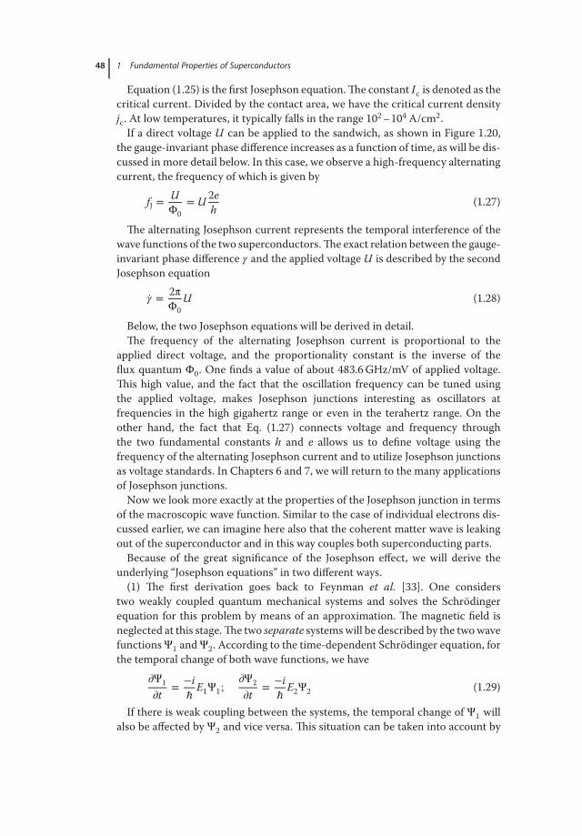
48 1 Fundamental Properties of Superconductors
Equation (1.25) is the first Josephson equation.The constant Ic is denoted as thecritical current. Divided by the contact area, we have the critical current densityjc. At low temperatures, it typically falls in the range 102–104 A/cm2.If a direct voltage U can be applied to the sandwich, as shown in Figure 1.20,
the gauge-invariant phase difference increases as a function of time, as will be dis-cussed in more detail below. In this case, we observe a high-frequency alternatingcurrent, the frequency of which is given by
fJ =UΦ0
= U 2eh
(1.27)
The alternating Josephson current represents the temporal interference of thewave functions of the two superconductors.The exact relation between the gauge-invariant phase difference 𝛾 and the applied voltage U is described by the secondJosephson equation
�� = 2πΦ0
U (1.28)
Below, the two Josephson equations will be derived in detail.The frequency of the alternating Josephson current is proportional to the
applied direct voltage, and the proportionality constant is the inverse of theflux quantum Φ0. One finds a value of about 483.6GHz/mV of applied voltage.This high value, and the fact that the oscillation frequency can be tuned usingthe applied voltage, makes Josephson junctions interesting as oscillators atfrequencies in the high gigahertz range or even in the terahertz range. On theother hand, the fact that Eq. (1.27) connects voltage and frequency throughthe two fundamental constants h and e allows us to define voltage using thefrequency of the alternating Josephson current and to utilize Josephson junctionsas voltage standards. In Chapters 6 and 7, we will return to the many applicationsof Josephson junctions.Now we look more exactly at the properties of the Josephson junction in terms
of the macroscopic wave function. Similar to the case of individual electrons dis-cussed earlier, we can imagine here also that the coherent matter wave is leakingout of the superconductor and in this way couples both superconducting parts.Because of the great significance of the Josephson effect, we will derive the
underlying “Josephson equations” in two different ways.(1) The first derivation goes back to Feynman et al. [33]. One considers
two weakly coupled quantum mechanical systems and solves the Schrödingerequation for this problem by means of an approximation. The magnetic field isneglected at this stage.The two separate systemswill be described by the twowavefunctionsΨ1 andΨ2. According to the time-dependent Schrödinger equation, forthe temporal change of both wave functions, we have
∂Ψ1∂t
= −iℏ
E1Ψ1;∂Ψ2∂t
= −iℏ
E2Ψ2 (1.29)
If there is weak coupling between the systems, the temporal change of Ψ1 willalso be affected by Ψ2 and vice versa. This situation can be taken into account by

1.5 Quantum Interference 49
introducing an additional coupling into Eq. (1.29):
∂Ψ1∂t
= −iℏ(E1Ψ1 + KΨ2) (1.30a)
∂Ψ2∂t
= −iℏ(E2Ψ2 + KΨ1) (1.30b)
In our case, the coupling means that Cooper pairs can be exchanged betweenthe superconductors 1 and 2. The coupling strength is symmetric and is fixed bythe constant K .Compared to other quantum mechanical systems with two states (for instance,
the H+2 molecule), a peculiarity of the two weakly coupled superconductors is the
fact that Ψ1 and Ψ2 describe macroscopic states occupied by a large number ofparticles.Thenwe can interpret the square of the amplitude in terms of the particledensity ns of the Cooper pairs. Hence, we can write
Ψ1 =√
ns1ei𝜑1 ; Ψ2 =√
ns2 ei𝜑2 (1.31)
Here, 𝜑1 and 𝜑2 are the phases of the wave functions Ψ1 and Ψ2, respectively.Inserting these wave functions into Eqs. (1.30a) and (1.30b), we obtain
ns1
2√
ns1ei𝜑1 + i
√ns1 ei𝜑1 × ��1 = − i
ℏ
{E1√
ns1 ei𝜑1 + K√
ns2 ei𝜑2}
(1.32a)
ns2
2√
ns2ei𝜑2 + i
√ns2 ei𝜑2 × ��2 = − i
ℏ
{E2√
ns2 ei𝜑2 + K√
ns1 ei𝜑1}
(1.32b)
By separating the real and the imaginary parts, we find
12
ns1√ns1
= Kℏ
√ns2 sin(𝜑2 − 𝜑1) (1.33a)
12
ns2√ns2
= Kℏ
√ns1 sin(𝜑1 − 𝜑2) (1.33b)
i√
ns1��1 = − iℏ{E1
√ns1 + K
√ns2 cos(𝜑2 − 𝜑1)} (1.34a)
i√
ns2��2 = − iℏ{E2
√ns2 + K
√ns1 cos(𝜑1 − 𝜑2)} (1.34b)
If we also take into account that, because of the exchange of Cooper pairsbetween 1 and 2, we must always have ns1 = −ns2, and if for simplicity we assumetwo identical superconductors (i.e., ns1 = ns2), from Eqs. (1.33a) and (1.33b) weobtain the differential equation
ns1 =2Kℏ
ns1 sin(𝜑2 − 𝜑1) = −ns2 (1.35)
The temporal change of the particle density in 1multiplied with the volumeV of1 yields the change of the particle number and, hence, the particle current across

50 1 Fundamental Properties of Superconductors
the junction. The electric current Is is obtained by multiplication of the particlecurrent with the charge 2e of each individual particle. Then we find
Is = Ic sin(𝜑2 − 𝜑1) (1.36)
with
Ic =2K × 2e
ℏV ns =
4πKΦ0
V ns (1.37)
This is the first Josephson equation, if we set the vector potentialA= 0.We recallthat we had neglected magnetic fields. Therefore, this step is justified. Turningfrom ns to the current within the junction, we must remember that both super-conductors are connected to a current source, which serves to keep ns constantwithin the superconductors by supplying or accepting the charges.From Eqs. (1.34a) and (1.34b) one obtains a differential equation for the tempo-
ral change of the phase difference. With ns1 = ns2 and E2 −E1 = 2eU , we have
ddt
(𝜑2 − 𝜑1) =2eUℏ
= 2πΦ0
U (1.38)
This is the second Josephson equation for the caseA= 0.We see that, for a tem-porally constant voltage U = constant, the phase difference increases linearly withtime:
𝜑2 − 𝜑1 =2πΦ0
Ut + 𝜑(t = 0) (1.39)
However, this means that according to the first Josephson equation an alter-nating current appears in the junction, the frequency f of which is given by Eq.(1.27).(2) The second derivation of the Josephson equations that we want to discuss
in part goes back to Landau and Lifschitz [34]. It is based only on very generalsymmetry and invariance principles and thereby emphasizes the wide range ofvalidity of the Josephson effect.We start by considering qualitatively how supercurrent density and phase are
connected to each other within a homogeneous superconducting wire.16) The cur-rent is assumed to flow in the z-direction. It is convenient towrite the supercurrentdensity as js,z = 2ensvz. We have used this relation already for the derivation of thefluxoid quantization. If we eliminate vz by using the canonical momentum, Eq.(1.5), we obtain
js,z =qm
ns(pcan,z − qAz)
or by using 𝐩can = ℏ𝐤
js,z =qm
ns(ℏkz − qAz)
16) These qualitative arguments treat the quantummechanics only in a rough way, but yield the correctresult.

1.5 Quantum Interference 51
Weconsider amatterwave of the formΨ=Ψ0 ei𝜑 =Ψ0 eik⋅x and, instead of kz, wewrite the expression 𝜑′ ≡ d𝜑/dz (the derivative of the phase 𝜑= k⋅x with respectto z yields kz). Then we obtain
js,z =qm
ns(ℏ𝜑′ − qAz) (1.40)
Now we define
𝛾(z) = 𝜑(z) −qℏ∫
z
0Az dz (1.41)
yielding
js,z =qℏm
ns × 𝛾 ′ (1.42)
What happens if our superconducting wire has a weakened location, where theCooper pair density is strongly reduced? This geometry is shown schematicallyin Figure 1.21. The current passing through the wire must have the same valueeverywhere. If we assume a constant supercurrent density over the cross-sectionof the wire, in Eq. (1.42) the product ns𝛾
′ must have the same value everywhere.However, if ns is strongly reduced at the weakened location, there 𝛾 ′ must bemuchlarger than in the remainder of the wire. If at the weakened location 𝛾 ′ displaysa sharp peak, 𝛾(z) changes there very rapidly from a value 𝛾1 to a much largervalue 𝛾2.
1.0
Is Is
0.5
0.0
−0.5
−1.0
−10 −5 0 5 10z
ns(z)
γ ′(z)
γ (z)
Figure 1.21 Derivation of the Josephsonequations. We consider a thin supercon-ducting wire with a weakened location atz = 0, at which the Cooper pair density nsis strongly reduced. Due to current conser-vation, we have ns(z)𝛾
′(z)= constant, lead-ing to a peak in 𝛾 ′(z) and to a step in 𝛾 . For
illustration we have used the following “testfunction”: ns(z)= 1/𝛾 ′(z)= 1/[1.001− tanh2(x)],constant= 0.001. For 𝛾(z) one finds𝛾(z)= tanh(z)+ 0.001z. At the weakenedlocation, 𝛾(z) changes very rapidly from −1to +1.

52 1 Fundamental Properties of Superconductors
Using Eq. (1.41), we can write the jump of the phase at the barrier as
𝛾 = 𝛾(z2) − 𝛾(z1) = 𝜑(z2) − 𝜑(z1) −qℏ∫
z2
z1Az dz (1.43)
where z1 denotes a coordinate in superconductor 1 in front of the barrier and z2a coordinate in superconductor 2 behind the barrier. Equation (1.43) has exactlythe same form as Eq. (1.26).If we specify the spatial dependence ns(z), the supercurrent across the barrier is
a function of the jump 𝛾 of the phase, that is, Is = Is(𝛾). However, a change of thephase difference of 2π should yield the same wave function and, hence, the samevalue of the supercurrent across the barrier. Therefore, we can expand Is as a sumof sine and cosine terms (a Fourier series):
Is(𝛾) =∞∑
n=0Icn sin(n𝛾) +
∞∑n=0
Icn cos(n𝛾) (1.44)
Here, Icn and Icn are the expansion coefficients of the function Is(𝛾). We note thatmicroscopic details such as the structure of the barrier or the temperature depen-dence of the Cooper pair density are contained in these expansion coefficients.However, the periodicity of Is(𝛾) is independent of this.Now we utilize the principle of time inversion symmetry. Many fundamental
phenomena in Nature are reversible. If we record such a phenomenon with acamera and then run the motion picture backward, we see again a process that isphysically possible.17) Nowwe assume that this principle also applies to the Joseph-son current. If the time is reversed, the current flows backward, that is, we have acurrent −Is. The macroscopic wave functions oscillate according to exp(−i𝜔t). Ifthe time is reversed here also, we see that also the sign of the phase of the wavefunction must be reversed. So if we request that the Josephson current be invari-ant under time reversal, we have the condition Is(𝛾)=−Is(−𝛾). This eliminates allthe cosine terms in Eq. (1.44).Under time inversion symmetry, the supercurrent across the barrier is described
by
Is(𝛾) =∞∑
n=0Icn sin(n𝛾) (1.45)
Very often, but not necessarily, one finds that this series converges very rapidly,that is, the expansion coefficients become smaller very quickly.Then the series canbe restricted to the first term, and we obtain the first Josephson equation.At this stage, we note that there are situations for which the first expansion
coefficient Ic1 vanishes, for example. In this case, the relation between the super-current and the phase difference 𝛾 has period π instead of 2π.
17) This is not valid for irreversible processes. A full glass of water falling to the ground breaks intomany pieces, and the water spreads over the floor. The inverse process, where the water and thebroken pieces jump upon the table and reassemble to an unbroken glass filled with water, onlyexists in the motion picture.

1.5 Quantum Interference 53
To obtain the second Josephson equation, we take the time derivative of Eq.(1.43), and we obtain
�� = ��(z2) − ��(z1) −qℏ∫
z2
z1Az dz (1.46)
According to the laws of electrodynamics, the integral over the time derivativeof the vector potential yields exactly the voltage induced across the barrierby a temporally changing magnetic field. The time derivative of the differ-ence 𝜑(z2)−𝜑(z1), with Ψ ∝ exp(−i𝜔t) = exp(−iEt∕ℏ), yields the difference[E(z2) − E(z1)]∕ℏ between the two superconductors on both sides of the barrier.We can write this difference as q U21, with the voltage difference U21. So wehave
�� =qℏ(U21 + Uind) =
qℏ
Utotal (1.47)
With q= 2e, this yields the second Josephson equation (1.28).The second derivation of the Josephson equations is very general. It was
assumed that there exists a macroscopic wave function with a well-defined phase𝜑, and that the system satisfies time inversion symmetry. Equations 1.40–1.47are also gauge-invariant.The gauge invariance represents a highly fundamental principle. In the force and
field equations of electrodynamics, only the electric and magnetic fields appear,not the corresponding potentials, the vector potential A and the scalar potentialΦ. From the latter, one obtains the (negative) electric field by forming the gra-dient. We have mentioned already that curlA=B. However, the magnetic fieldis source-free, that is, we have divB= 0. Therefore, a vector V(x,y,z,t), obtainedfrom the gradient of a function 𝜒(x, y, z, t), can be added to A. This correspondsto a different scaling of A. The curl of V always vanishes, and, hence, the mag-netic field remains unaffected. However, in order also to keep the electric fieldunchanged during this transformation, at the same time we must subtract thequantity 𝜒(x,y,z,t) from the scalar potential. Finally, in the Schrödinger equation,the phase 𝜑 of the wave function must be rescaled to 𝜑+ (2π/Φ0)𝜒 . The gaugeinvariance of Eqs. (1.40–1.47) can be shown by explicitly inserting these relations.Often, equations showing gauge invariance are of fundamental importance in
physics and cannot be affected easily bymicroscopic details. Hence, we can expectthat the Josephson equations are generally valid in the case ofmany different typesof barriers and superconductors.In Figure 1.22, some types of junctions are shown schematically. For the
superconductor–insulator–superconductor (SIS) junction (Figure 1.22a), theinsulating barrier must be only 1–2 nm thick. The superconductor–normalconductor–superconductor (SNS) junction (Figure 1.22b) can function witha much larger thickness of the normal conductor, simply because the Cooperpairs can penetrate much deeper into a normal conducting metal than intoan oxide layer. Here, in the normal metal, the decay length of the Cooper pairconcentration depends among other things on the electron mean free path. Forvery large values of the electron mean free path (small amount of perturbations),

54 1 Fundamental Properties of Superconductors
S
S
(a) (b)
(c) (d)
(e)
Bi2Sr2CaCu2O8
S
S
S
I
ICuO
BiSr
Ca
(f)
Insulator
Substrate
Superconductor SuperconductorNormalconductor
Substrate
Figure 1.22 Schematics of the differentpossibilities for producing a weak cou-pling between two superconductors: (a) SISjunction with an oxide layer as a barrier;(b) SNS junction with a normal conducting
barrier; (c) point contact; (d) microbridge;(e) YBa2Cu3O7 grain boundary junction;and (f ) intrinsic Josephson junction inBi2Sr2CaCu2O8.
normal conducting layers with a thickness up to a few hundred nanometers canbe used. An important difference between the oxide and the normal conductorjunctions is the value of the resistance per square (normal resistance/area ofthe barrier). For the oxide junctions, the value of the resistance per square istypically 10−4–10−3 Ω cm2. However, for the SNS junctions, this value is about10−8 Ω cm2 or below. In addition to the SIS and SNS junctions, one often alsouses junctions with a more complicated structure of the barrier, for instance, theso-called SINIS junctions where the barrier is formed by two insulators and onenormal conducting layer.The point contacts (Figure 1.22c) are particularly simple. In this case, a metal tip
is pressed against a surface.The cross-section of the bridge depends on the appliedpressure. In this way, the desired junction properties can be produced easily andcan be adjusted if necessary. The microbridge (Figure 1.22d) only consists of anarrow constriction that limits the exchange of Cooper pairs because of its verysmall cross-section. Here, it is necessary to fabricate reproducibly bridges with

1.5 Quantum Interference 55
a width of only 1 μm or smaller, which requires advanced structuring techniquessuch as electron beam lithography.For the high-temperature superconductors, one can use grain boundaries as
weak coupling regions because of the small values of the coherence length [35,36]. One can deposit a thin film, say, of YBa2Cu3O7 on a “bicrystal substrate,” con-sisting of two single-crystalline parts joined together at a specific angle. The grainboundary of the substrate is then transferred also into the deposited film, whichotherwise is grown single-crystalline (epitaxially, Figure 1.22e).Well-defined grainboundaries can also be produced at steps in the substrate or at the edges of bufferlayers epitaxially deposited on a substrate.The strength of the Josephson couplingcan be varied over a large range by means of the grain boundary angle.In some high-temperature superconductors such as, for instance,
Bi2Sr2CaCu2O8, even intrinsic Josephson junctions exist simply because oftheir crystal structure (Figure 1.22f ). Here, the superconductivity is restrictedonly to the copper oxide layers with about 0.3 nm thickness. Between these layers,there are electrically insulating bismuth oxide and strontium oxide planes. Hence,such materials form stacks of SIS Josephson junctions, where each junction hasa thickness of only 1.5 nm, the distance between two neighboring copper oxidelayers [37].These highly different types of Josephson junctions only represent a small
selection of the many possibilities. Each type of junction has its advantages anddisadvantages. Depending on the specific application, quite different types canbe utilized.At this stage, we are confrontedwith the following question: How similar are the
Josephson effects in these junctions, in particular, with respect to the connectionbetween the oscillation frequency of the alternating Josephson currents and theapplied voltage? The proportionality factor 1/Φ0, which is also referred to18) asthe “Josephson constant” K J = 2e/h= 483.5979GHz/mV, has been determined formany different types of Josephson junctions. For example, a Josephson junctionmade of indium with its weak location realized by a constriction (microbridge)has been compared directly with a Josephson junction made of niobium wherethe barrier consisted of a thin gold layer [38]. The Josephson constants measuredfor both junctions were equal within an uncertainty of only 2× 10⁻¹⁶ or less. Inthe meantime, this accuracy could be increased even to about 10−19. Therefore,Josephson junctions are now applied for representing the voltage standard [39].How can we demonstrate alternating Josephson currents experimentally? A
very direct method is the observation of the electromagnetic radiation generatedby the oscillating Josephson currents in the frequency range of microwaves. Wewant to estimate the order of magnitude of the microwave power emitted fromthe junction.We assume a voltage of 100 μV applied to the junction, corresponding to an
emitted frequency of about 48GHz. The critical current Ic of the junction is
18) The value given here was defined internationally in 1990 as the Josephson constant K J-90, and there-fore is exact.

56 1 Fundamental Properties of Superconductors
assumed to be 100 μA.Then the d.c. power applied to the junction is 10−8 W, andthe emitted power is expected to be much smaller than this value.The difficulty of direct experimental demonstration did not so much arise
because of the small power of this radiation, but, instead, it had to do with theproblem of coupling the high-frequency power from the tiny tunnel junctioninto a proper high-frequency waveguide. Therefore, the first confirmation of thealternating Josephson current came in an indirect way [40]. If such a junction isplaced within the high-frequency field of an oscillating microwave cavity, charac-teristic, equidistant steps of constant voltage are observed in the voltage–currentcharacteristic (see Section 6.3). On the voltage axis, their distance ΔU is given by
ΔUS = Φ0 × fHF (1.48)
where f HF is the frequency of the high-frequency field.These “Shapiro steps” resultfrom the superposition of the alternating Josephson current and the microwavefield. Each time that the frequency of the alternating Josephson current corre-sponds to an integer multiple of the microwave frequency, the superposition pro-duces an additional d.c. Josephson current, causing the step structure of the char-acteristic.Another indirect confirmation of the existence of an alternating Josephson cur-
rent was found for junctions placed within a small static magnetic field. Here, atsmall voltages Us, equidistant steps in the characteristic could be observed with-out irradiation by an external high-frequency field (see Section 6.4).The sandwichgeometry of a Josephson tunnel junction by itself represents a resonating cavity,and the structures observed in the characteristic, the “Fiske steps,” correspond toresonances within the junction. For the proper values of the voltage Us and of thefield B, the Josephson oscillations of the current density exactly fit a cavity modeof the junction. For such a resonance, the current becomes particularly large.A more accurate description of the Shapiro and Fiske modes requires a math-
ematical treatment beyond the scope of this first chapter. However, in Chapter 6,we will return to these structures.In 1965 Ivar Giaever19) achieved a more direct confirmation of the alternating
Josephson current [41]. As we have seen, the main difficulty with the direct con-firmation, say, with a typical high-frequency apparatus, arose from the extractionof power out of the small tunnel junction. Giaever had the idea that a second tun-nel junction, placed immediately on top of the Josephson junction, would be quitefavorable for such an extraction (Figure 1.23).Here, the confirmation of the extracted power happens in the second tunnel
junction by means of the change of the characteristic of the tunneling current forindividual electrons, this change being caused by the irradiating high-frequencyfield generated in the Josephson junction. In the years prior to this, it had beenshown that a high-frequency field generates a structure in the characteristic of the
19) For his experiments with superconducting tunnel junctions, Giaever received the Nobel Prize in1973, together with B. D. Josephson and L. Esaki.

1.5 Quantum Interference 57
= =
===
==
==
=
=
==
===
==
=
=
==
= =
=
=
==
==
===
=
1 2
Us
U2–3 I
3 a b
Figure 1.23 Arrangement for the exper-imental demonstration of the alternatingJosephson current according to Giaever:layers 1–3 are Sn layers; layers a and b areoxide layers. The thicknesses of layers a
and b are chosen such that layers 1 and 2form a Josephson junction, and such thatno Josephson currents are possible betweenlayers 2 and 3. (From [40].)
single-electron-tunneling current [42]. The electrons can interact with the high-frequency field by absorbing or emitting photons with energy E = hf HF.In Section 3.1.3wewill see that, in the absence of a high-frequency field, individ-
ual electrons can tunnel in large numbers between the two superconductors onlyafter the voltage (Δ1 +Δ2)/e has been reached. Here,Δ1 andΔ2 denote the energygaps of the two superconductors, respectively, the magnitudes of which dependon the material. In other words, during the tunneling process, the electrons musttake up at least the energy eU = (Δ1 +Δ2). Then at the voltage (Δ1 +Δ2)/e, thevoltage–current characteristic displays a sharp step as seen in Figure 1.23.In a high-frequency field, a tunneling process assisted by photons can set in
already at the voltage Us = (Δ1 +Δ2 − hf HF)/e. If during a tunneling process anelectron absorbs several photons, one obtains a structure in the characteristic withthe specific interval of the voltage Us
ΔUs =hfHF
e(1.49)
where h is the Planck’s constant, f HF is the frequency of the high-frequency field,and e is the elementary charge. Such processes can happen at high photon den-sities, that is, at high power of the high-frequency field. We note that for single-electron tunneling, the elementary charge e of single electrons appears.At the junction 2–3, one observes a typical single-electron characteristic if no
voltage is applied to the junction 1–2 (curve 1 in Figure 1.24). For performingthe key experiment, a small voltage Us is applied to the Josephson junction 1–2.If the expected high-frequency alternating current appears in this junction, inthe junction 2–3 the well-known structure of the tunneling characteristic shouldbe observed, because of the close coupling between the two junctions. Giaever,indeed, could observe this expected effect. Such a characteristic is shown by curve2 in Figure 1.24. Here a voltage Us of 0.055mV was applied to junction 1–2,

58 1 Fundamental Properties of Superconductors
1.5
T ≃ 1.2K
2Us
1.0
Cu
rre
nt
l 2-3
in m
A
0.5
00.5 1.0
1
2
1.5
Voltage U2-3 in mV
Figure 1.24 Characteristic of the junction 2–3 from Figure 1.22. Curve 1: no voltage atjunction 1–2. Curve 2: 0.055mV applied to junction 1–2.
acting as the generator of the high-frequency field. The frequency of the alter-nating Josephson current is f J = 2eUs/h, and the structure of the characteristicof junction 2–3 should display the voltage steps with the distance between themΔUs = hf J/e= 2Us. For the curve shown in Figure 1.24, this yieldsΔU2,3 = 0.11mV,which was observed by Giaever.The most direct detection of the alternating Josephson current by coupling the
power into a high-frequency waveguide has been achieved by an American and aRussian group.The Americans [43] could detect the high-frequency power of theJosephson junction by placing the junction into a tuned resonating cavity, whichwas operated at a resonance frequency of the junction by choosing a proper valueof themagnetic field. However, this still required an extremely high detection sen-sitivity. The detected power was about 10−11 W, whereas the sensitivity limit fordetection could be increased up to 10−16 W.The Russian group, Yanson et al. [44],could detect a radiation power of about 10−13 W of a Josephson junction.The rela-tion f J = 2eUs/h has always been found between the frequency of the alternatingJosephson current and the voltage applied to the junction.The experimental accu-racy has been increased by the American group sufficiently far that a precisionmeasurement of 2e/h could be carried out [45].This represented further convinc-ing proof of the importance of electron pairs in superconductivity.Today, the techniques for the detection of electromagnetic radiation are
improved to such an extent that the alternating Josephson current can be extractedwithout any difficulty up to the 100GHz range. However, there are still problemsat frequencies in the terahertz range, which play an important role, for instance,in the intrinsic Josephson junctions of high-temperature superconductors.In the meantime, also this emission was detected. [54, 55]

1.5 Quantum Interference 59
In the future, Josephson junctions are expected to play an important role in theterahertz range. On the one hand, this frequency range is too high to be coveredby semiconductor devices, and on the other, it is too low to be handled by opticalmethods.
1.5.2Quantum Interference in a Magnetic Field
In the alternating Josephson currents, the macroscopic wave function manifestsitself in the form of a temporal interference between the matter waves in the twosuperconducting electrodes. What can we say about the spatial interference, say,analogous to the optical double-slit experiment or to the Sagnac interferometer?Let us look at the structure shown in Figure 1.25. It consists of a superconduct-
ing ring into which two Josephson junctions are integrated.The ring is located in amagnetic field oriented perpendicular to the area of the ring. A transport currentI flows along the ring. By measuring the voltage drop across the Josephson junc-tions, we can determine the maximum supercurrent that can be carried by thering. We will see that this maximum supercurrent Is,max oscillates as a function ofthe magnetic flux through the ring, similar to the light intensity, or more exactlythe light amplitude, on the screen of the double-slit experiment, and also similarto the Sagnac interferometer with its dependence on the rotational frequency.In Section 1.3, we looked at a superconducting ring placed in a magnetic field
and we found that the magnetic flux through the ring appears in multiples of theflux quantumΦ0. An arbitrary magnetic field Ba could be applied to the ring, gen-erating an arbitrarymagnetic fluxΦa through the ring. However, in this case, a cir-culating current J flows along the ring. It also generates a magnetic fluxΦind = LJ ,
Current
1 2 Voltage
(a) (b)
B-Field
I
I
J
Ba
I1
1
1′ 2′2
I2
Current
Figure 1.25 Generation of spatial interferences of the superconducting wave function ina ring structure. (a) Schematics of the wave. (b) Notation for the derivation of the quantuminterference.

60 1 Fundamental Properties of Superconductors
such that the total flux amounts to amultiple ofΦ0:Φtot =Φa + LJ .The circulatingcurrent results in a shift of Φa upward or downward to the next integer value ofΦtot/Φ0. Apparently, LJ must then reach a maximum value up to Φ0/2.This picture is changed because of the insertion of the two Josephson junctions.
At both Josephson junctions, the phase of the superconducting wave function canjump by amounts 𝛾1 or 𝛾2, which must be taken into account in the integrationof the phase gradient around the ring (integral ∮ 𝐤d𝐱). The jumps of the phaseare connected with the current across the junctions because of the first Josephsonequation (1.25).Next, we derive the dependence Is,max(Φa) using the notation of Figure 1.25b.
We assume that the width of the Josephson junctions is much smaller than thediameter of the ring. The current I separates into the currents I1 and I2, flowingalong the two halves of the ring, respectively. Because of current conservation, wehave
I = I1 + I2 (1.50)
The currents I1 and I2 can also be written in terms of the circulating current Jflowing in the ring yielding
I1 =I2+ J; I2 =
I2− J (1.51)
The current I1 flows through the Josephson junction 1, and the current I2through the Josephson junction 2. Therefore, we have
I1 = Ic sin 𝛾1; I2 = Ic sin 𝛾2 (1.52)
Here, for simplicity, we have assumed that the critical currents Ic of the twoJosephson junctions are identical. Therefore, we find
I2+ J = Ic sin 𝛾1 (1.53a)
I2− J = Ic sin 𝛾2 (1.53b)
Next, we need a relation connecting the gauge-invariant phase differences 𝛾1and 𝛾2 with the applied magnetic field. We proceed analogously to the derivationof the quantization of the fluxoid (Eq. (1.11)), but we do not integrate the wavevector k over the complete ring, as in Eq. (1.7). Instead, we integrate separatelyover the lower and upper halves, that is, from 1′ to 2′ or from 2 to 1 in Figure 1.25b.Then we obtain
∫2′
1′𝐤d𝐫 = 𝜇0𝜆
2L∫
2′
1′𝐣s d𝐫 +
2πΦ0 ∫
2′
1′𝐀d𝐫 (1.54a)
∫1
2𝐤d𝐫 = 𝜇0𝜆
2L∫
1
2𝐣s d𝐫 +
2πΦ0 ∫
1
2𝐀d𝐫 (1.54b)
Here, we have used the definition 1.10 of the London penetration depth andΦ0 = h/q= h/2e.

1.5 Quantum Interference 61
The integral ∫2′
1′𝐤d𝐫 yields the difference between the phase 𝜑2 of the wave
function of the lower half of the ring, Ψ2 ∼ exp(ik⋅r)= exp(i𝜑2) at the locations
2′ and 1′, ∫2′
1′𝐤d𝐫 = 𝜑2(2′) − 𝜑2(1′). Analogously, one finds ∫
1
2𝐤d𝐫 = 𝜑1(1) −
𝜑1(2). By adding Eqs. (1.54a) and (1.54b), we obtain
𝜑2(2′) − 𝜑1(2) − [𝜑2(1′) − 𝜑1(1)] = 𝜇0𝜆2L
(∫
2′
1′𝐣s d𝐫 + ∫
1
2𝐣s d𝐫
)+ 2π
Φ0∮C′𝐀d𝐫
(1.55)
Here, the integral over the curveC′ does not include the barriers of the two Joseph-son junctions. Otherwise, the integral would run over the complete ring, and byusing Stokes’ theorem we could turn it into the magnetic flux through the ring.However, we can accomplish this by adding the integrals over the correspondingdistances on both sides of Eq. (1.55). Then we find
∮C′𝐀d𝐫 + ∫
2
2′𝐀d𝐫 + ∫
1′
1𝐀r d𝐫 = ∮C
𝐀d𝐫 = ∫F𝐁d𝐟 = Φ (1.56)
On the left-hand side of Eq. (1.55), the term
𝜑2(2′) − 𝜑1(2) +2πΦ0 ∫
2
2′𝐀d𝐫
yields the gauge-invariant phase difference 𝛾2 across the Josephson junction 2.Analogously, the expression
𝜑2(1′) − 𝜑1(1) −2πΦ0 ∫
1′
1𝐀d𝐫
yields the gauge-invariant phase difference 𝛾1 across the Josephson junction 1. Inthis way, we find
𝛾2 − 𝛾1 = 𝜇0𝜆2L
(∫
2′
1′𝐣s d𝐫 + ∫
1
2𝐣s d𝐫
)+ 2π
Φ0Φ (1.57)
Similar to the case of a massive circular ring, the magnetic flux Φ is given bythe sum of the applied flux Φa and the self-field of the circulating currents J:Φ=Φa + LJ . The contributions of the current densities are proportional to thecirculating current J and can be included in the term LJ .20) Finally, we obtain therelation we had been looking for
𝛾2 − 𝛾1 =2πΦ0
Φ = 2πΦ0
(Φa + LJ) (1.58)
20) Therefore, the inductivity of the ring is slightly increased.This contribution is referred to as “kineticinductance” Lkin, which must be added to the inductance L given by the geometry. Hence, we haveLtot = L+ Lkin. However, since mostly the contribution Lkin is very small, we will not distinguish anyfurther between Ltot and L.

62 1 Fundamental Properties of Superconductors
From Eqs. (1.53a), (1.53b) and (1.58), we can calculate the maximum supercur-rent along the ring as a function of the applied magnetic field or of the flux.Let us start by assuming that we can neglect the contribution of the term LJ
to the magnetic flux. The circulating current J clearly cannot become larger thanthe critical current Ic of the Josephson junctions. Hence, the flux generated by theterm LJ is smaller than LIc. We assume also that this flux is much smaller thanhalf a flux quantum, yielding the condition 2LIc∕Φ0 ≪ 1. The quantity 2LIc/Φ0 isreferred to as the inductance parameter 𝛽L,
𝛽L =2LIcΦ0
(1.59)
If we neglect the magnetic flux generated by the circulating current, we haveΦ=Φa. Using Eq. (1.58), we eliminate 𝛾2 from Eqs. (1.53a) and (1.53b). Then, byadding Eqs. (1.53a) and (1.53b), we obtain
I = Ic[sin 𝛾1 + sin
(2π
ΦaΦ0
+ 𝛾1
)](1.60)
Now it is advantageous to use the variable 𝛿 = 𝛾1 +π(Φa/Φ0) instead of 𝛾1.ThenEq. (1.60) can be changed into
I = Ic[sin
(𝛿 − π
ΦaΦ0
)+ sin
(𝛿 + π
ΦaΦ0
)](1.61)
By using the trigonometric identity for the summation of sines, we obtain theexpression
I = 2Ic sin 𝛿 cos(πΦaΦ0
)(1.62)
If we specify the flux Φa and the current I, the variable 𝛿 will adjust itself suchthat Eq. (1.62) is satisfied. For increasing current, this is possible at most up to thepoint where sin 𝛿 becomes equal to +1 or −1, depending on the current directionand on the sign of the cosine factor. Hence, the maximum supercurrent that canflow through this circular structure is given by
Is,max = 2Ic|||||cos
(πΦaΦ0
)||||| (1.63)
The quantity Is,max reaches a maximum if the flux corresponds to an integermultiple of a flux quantum. Then the cosine factor is equal to 1, and we obtainIs,max = 2Ic. This is the maximum supercurrent that can be carried by the parallelconfiguration of the two Josephson junctions. In this case, we have sin 𝛾1 = sin𝛾2 = 1. In this case, the circulating current J , obtained as
J =Ic2(sin 𝛾1 − sin 𝛾2) (1.64)
by subtraction of Eqs. (1.53a) and (1.53b), vanishes. The current Is,max vanisheseach time that Φa reaches the value (n + 1∕2) Φ0 with n= 0, ±1, ±2, … Now thecirculating current attains its maximum value, becoming equal to +Ic or −Icdepending on the value of n.

1.5 Quantum Interference 63
Themaximum supercurrent flowing within the circular structure also oscillatesperiodically as a function of the applied magnetic field. Here, the period of themagnetic flux generated by the field is the magnetic flux quantum.This effect wasfirst demonstrated experimentally byMercereau and coworkers [46]. It is the anal-ogy of the diffraction of light by a double slit, and it represents the foundation ofthe application of such circular structures as a superconducting quantum inter-ferometer (SQUID). We note that SQUIDs can measure an applied magnetic fieldcontinuously.SQUIDs will be discussed in detail in Section 7.6.4. However, at this stage, we
point out already that SQUIDs can resolve changes of the magnetic flux down toabout 10−6Φ0. If the area of the SQUID is about 1mm2, then this corresponds tofield changes ΔB of about 10−6Φ0/mm2 = 10−15 T, which can be detected with aSQUID.This value is smaller than the Earth’s magnetic field by 11 orders of magnitude,
and approximately corresponds to the magnetic fields generated at the surface ofthe skull by the electric currents within the human brain. SQUIDs belong to thegroup of most sensitive detectors by far. Since the measurement of many physicalquantities can be transformed into amagnetic field or fluxmeasurement, SQUIDsfind very wide applications.Again, we can briefly discuss the analogy with the Sagnac interferometer. If in
a constant external magnetic field the SQUID is rotating around an axis perpen-dicular to the area of the ring, a phase shift of (2m∕ℏ)2πR2Ω = 4π2R2(2m∕h)Ωresults in the interferometer. Here, Ω is the angular velocity and 2m is the massof a Cooper pair. We have assumed a circular SQUID with radius R. Hence,Is,max oscillates with a period depending on the ratio m/h. Already by 1950,Fritz London had pointed out the equivalence of a rotating superconductor andan externally applied magnetic field [47]. A similar rotational effect can alsobe observed with other coherent matter waves, for instance, with superfluidhelium [48]. However, since the mass of helium atoms is much larger than that ofCooper pairs, for helium the sensitivity against rotation is much larger than forSQUIDs.Next, we discuss briefly the approximations leading us to Eq. (1.63). We had
assumed that the critical currents Ic of both Josephson junctions are identical.Without this assumption, we would find that Is,max varies between Ic1 + Ic2 and|Ic1 − Ic2|, where again the period is one flux quantum. So compared to Eq. (1.63),there is no qualitative change. Furthermore, the period of the oscillation remainsunchanged if the finite inductance is taken into account. As before, the maximumvalue Is,max is again given by Ic1 + Ic2. However, the minimum value of Is,max(Φ)more andmore approaches themaximumvalue. In Figure 1.26, we show this effectfor three different values of the inductance parameter 𝛽L.For large values of the inductance parameter 𝛽L, the relative modulation ampli-
tude decreases proportional to 1/𝛽L. In order to see this, we must rememberthat for a massive superconducting ring, a shielding current with a maximumvalue of J =Φ0/2L was sufficient to supplement the applied flux until it reachedthe next integer value of Φ0. If we apply this principle to the SQUID, the

64 1 Fundamental Properties of Superconductors
2
1
I s,m
ax/I c
00.0 0.5 1.0 1.5
ϕ/ϕ0
0.01
βL
1
5
2.0
Figure 1.26 Modulation of the maximum supercurrent of a superconducting quantuminterferometer as a function of the magnetic flux through the ring. The curves are shownfor three different values of the inductance parameter 𝛽L.
circulating current must not exceed the value Φ0/2L. For large values of theinductance, this circulating current is smaller than Ic, and Is,max is reduced tothe value 2(Ic − J). Therefore, we obtain a relative modulation amplitude of[2Ic − 2(Ic − J)]/2Ic = J/Ic =Φ0/(2LIc)= 1/𝛽L. Hence, the effect of the quantuminterference decreases with increasing inductance.If we include thermal fluctuation effects, one can show that the optimum sen-
sitivity of SQUIDs against flux changes is reached for 𝛽L = 1. However, for a givenvalue of the critical current, this also limits the area of the SQUID ring, since theinductance increases with increasing circumference of the ring. Hence, on the onehand, one desires an area as large as possible in order to achieve a large change offlux with a small change of the magnetic field. On the other hand, this area cannotbe too large, because otherwise the inductance would become too large.This con-flict has resulted in a number of highly special SQUID geometries, which deviatestrongly from the simple ring structure shown in Figure 1.25.Wewill discuss thesegeometries in Section 7.6.4.Finally, we turn to the effects resulting from the finite size of the Josephson junc-
tions. We will see that also the critical current of the junctions depends on themagnetic field or on the magnetic flux through the junction, in analogy to thediffraction of light at a double slit.Let us look at the geometry of a spatially extended Josephson junction shown
schematically in Figure 1.27. We assume that this junction is penetrated by amagnetic field along the z-direction parallel to the barrier layer. We look for anequation describing the dependence of the gauge-invariant phase difference 𝛾 onthe applied magnetic field. For the superconducting ring of Figure 1.25, we sawthat the difference 𝛾2 − 𝛾1 of the two phases of the Josephson junctions, assumedto represent point junctions, is proportional to the magnetic flux enclosedbetween these junctions.In analogy to the earlier derivation of the relevant equations, we look at the path
along which we want to integrate the wave vector of the superconducting wavefunction. In Figure 1.27, this path is shown as the dotted line. Along the x-axis

1.5 Quantum Interference 65
I
ba
x
z
Ba
1
1′ 2′
2
Figure 1.27 Geometry of the spatially extended Joseph-son junction.
the path extends from point x to point x+ dx, where dx denotes an infinitesimallysmall distance. Along the y-direction the path extends deeply into the interior ofboth superconductors, for which we assume that they are much thicker than theLondon penetration depth. In analogy to Eq. (1.57), we find
𝛾(x + dx) − 𝛾(x) = 𝜇0𝜆2L
(∫
2′
1′𝐣s d𝐫 + ∫
1
2𝐣s d𝐫
)+ 2π
Φ0Φ1 (1.65)
Here,ΦI denotes the total flux enclosed by the integration path. Beyond a layer ofdepth 𝜆L, the shielding currents in the superconducting electrodes are exponen-tially small. Therefore, we can neglect the two integrals taken over the supercur-rent densities. Furthermore, we assume that the supercurrents and the magneticfields vary along the x-direction, but not along the y-direction. Then we write forthe magnetic flux
Φ1 = B teff dx (1.66)
We find the “effective thickness” teff by integrating the magnetic field along thez-direction. Since the magnetic field decays exponentially in the two supercon-ductors within a characteristic length 𝜆L, this integration yields
teff = 𝜆L,1 + 𝜆L,2 + tb (1.67)
Here, 𝜆L,1 and 𝜆L,2 are the London penetration depths in the two superconductors,respectively. They do not have to be identical. The thickness of the barrier layer isdenoted by tb. In general, it is much smaller than 𝜆L,1 and 𝜆L,2. Hence, mostly itcan be neglected.With these assumptions and notations, fromEq. (1.65) we obtain the differential
equation
𝛾 ′ ≡ d𝛾dx
= 2πΦ0
Bteff (1.68)
yielding the connection we had been looking for.Furthermore, we assume that we can neglect the self-field generated by the
Josephson currents. This assumption represents a condition about the spatialextension of the junction along the x and y directions. In Section 6.4, we will see

66 1 Fundamental Properties of Superconductors
that it is necessary that the lengths a and b of the edges of the junction do notexceed the so-called Josephson penetration depth
𝜆J =
√Φ0
2π𝜇0jcleff(1.69)
Here, jc is the critical supercurrent density, assumed to be spatially homogeneous,and the length leff is equal to teff if the superconducting electrodes aremuch thickerthan 𝜆L, as we had assumed. Typically, the Josephson penetration depth is a fewmicrometers. However, it can also increase up to themillimeter scale if the criticalsupercurrent density is very small.With the assumptions indicated earlier, themagnetic fieldB is equal to the exter-
nally applied field Ba. Then we can integrate Eq. (1.68) and obtain
𝛾(x) = 𝛾(0) + 2πΦ0
Bateffx (1.70)
The gauge-invariant phase difference is seen to increase linearly with thex-coordinate. Inserting this function 𝛾(x) into the first Josephson equation, weobtain for the spatial dependence of the supercurrent density across the barrierlayer
js(x) = jc sin[𝛾 (0) + 2π
Φ0Bateffx
](1.71)
We see that the supercurrent density oscillates along the x-coordinate, that is,perpendicular to the applied field. Here, the wavelength of the oscillation is deter-mined by the applied magnetic field.Now we want to calculate the maximum Josephson current that can flow across
the Josephson junction. For this we integrate Eq. (1.71) over the area of the junc-tion:
Is = ∫b
0dy∫
a
0dx jc sin
[𝛾 (0) + 2π
Φ0Bateffx
](1.72a)
Next we assume that the critical supercurrent density jc is spatially homoge-neous, that is, it is independent of x and y. Then the integration yields
Is = jcb∫a
0dx sin
[𝛾 (0) + 2π
Φ0Bateffx
]= −jc b
cos[𝛾 (0) + 2π
Φ0Bateffx
]2πΦ0
Bateff
|||||||a
0
(1.72b)
Inserting the integration limits, we obtain
Is = jcbcos 𝛾(0) − cos
[𝛾 (0) + 2π
Φ0Bateffa
]2πΦ0
Bateff(1.72c)
With the variable 𝛿 = 𝛾(0)+ (π/Φ0)Bateffa and using the relation cos(𝛼 ± 𝛽)= cos𝛼 cos 𝛽 ∓ sin 𝛼 sin 𝛽, finally we find
Is = jcab sin 𝛿sin
[πΦ0
Bateffa]
πΦ0
Bateffa(1.72d)

1.5 Quantum Interference 67
Similar to Eq. (1.62), for a given current I and magnetic field Ba, the quantity 𝛿will adjust itself in such away that Eq. (1.72d) will be satisfied.This is possible up tothe value for which sin 𝛿 =±1, and finally we obtain themagnetic field dependenceof the critical current of the Josephson junction
Ic(ΦJ) = Ic(0)|||||||sin
[π ΦJ
Φ0
]π ΦJ
Φ0
||||||| (1.73)
where 𝛷J =Bateffa and Ic(0)= jcab. The quantity 𝛷J corresponds to the magneticflux penetrating the Josephson junction.The function 1.73 is shown in Figure 1.28a. In analogy to the diffraction of light
by a slit, it is referred to as a Fraunhofer pattern. In Figure 1.28b, we see the mea-sured dependence Ic(Ba) for a Sn–SnO–Sn tunnel junction. With a value of theLondon penetration depth of 30 nm, one obtains for teff a value of about 60 nm.The width of the junction was 250 μm. Hence, we expect zero values of the crit-ical current within a distance ΔBa =Φ0/(ateff)≈ 1.4G. This agrees well with theexperimental result ΔBa = 1.25G.If the critical current density jc had been inhomogeneous, that is, depending
upon the spatial coordinates x and y, the function Ic(Ba) would have deviatedstrongly from the form of the Fraunhofer pattern. Therefore, the measure-ment of Ic(Ba) often serves as a simple test of the homogeneity of the barrierlayer.What about the physics behind the Fraunhofer pattern? For light diffraction by
a slit, minima in the interference stripes appear at locations where the waves pass-ing through the slit interfere destructively with each other. According to Eq. (1.70),in the Josephson junction the magnetic field causes an increase in the gauge-invariant phase difference along the barrier, and the supercurrent density spatially
1.0
Φ/Φ0
I o(Φ
)/I o
(0)
0.5
30
Maxim
um
. superc
urr
ent in
mA
Magnetic field in Gauss
25
20
15
10
5
0 2 4 6 8
0.00 1 2 3 4
(a) (b)
5
Figure 1.28 Dependence of the maximum Josephson current on the magnetic field paral-lel to the barrier layer. (a) Theoretical curve according to Eq. (1.73). (b) Measured data for aSn–SnO–Sn tunnel junction (1 G= 10−4 T). .(From [49].)
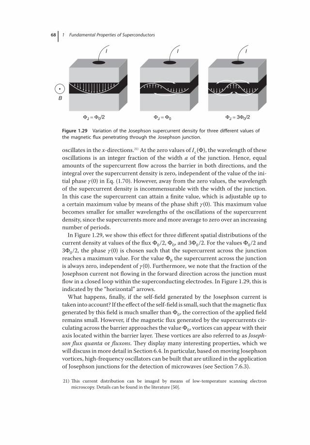
68 1 Fundamental Properties of Superconductors
I
B
ΦJ = Φ0/2 ΦJ = Φ0 ΦJ = 3Φ0/2
I I
Figure 1.29 Variation of the Josephson supercurrent density for three different values ofthe magnetic flux penetrating through the Josephson junction.
oscillates in the x-directions.21) At the zero values of Ic(Φ), the wavelength of theseoscillations is an integer fraction of the width a of the junction. Hence, equalamounts of the supercurrent flow across the barrier in both directions, and theintegral over the supercurrent density is zero, independent of the value of the ini-tial phase 𝛾(0) in Eq. (1.70). However, away from the zero values, the wavelengthof the supercurrent density is incommensurable with the width of the junction.In this case the supercurrent can attain a finite value, which is adjustable up toa certain maximum value by means of the phase shift 𝛾(0). This maximum valuebecomes smaller for smaller wavelengths of the oscillations of the supercurrentdensity, since the supercurrents more andmore average to zero over an increasingnumber of periods.In Figure 1.29, we show this effect for three different spatial distributions of the
current density at values of the flux Φ0/2, Φ0, and 3Φ0/2. For the values Φ0/2 and3Φ0/2, the phase 𝛾(0) is chosen such that the supercurrent across the junctionreaches a maximum value. For the value Φ0 the supercurrent across the junctionis always zero, independent of 𝛾(0). Furthermore, we note that the fraction of theJosephson current not flowing in the forward direction across the junction mustflow in a closed loop within the superconducting electrodes. In Figure 1.29, this isindicated by the “horizontal” arrows.What happens, finally, if the self-field generated by the Josephson current is
taken into account? If the effect of the self-field is small, such that themagnetic fluxgenerated by this field is much smaller thanΦ0, the correction of the applied fieldremains small. However, if the magnetic flux generated by the supercurrents cir-culating across the barrier approaches the valueΦ0, vortices can appear with theiraxis located within the barrier layer. These vortices are also referred to as Joseph-son flux quanta or fluxons. They display many interesting properties, which wewill discuss inmore detail in Section 6.4. In particular, based onmoving Josephsonvortices, high-frequency oscillators can be built that are utilized in the applicationof Josephson junctions for the detection of microwaves (see Section 7.6.3).
21) This current distribution can be imaged by means of low-temperature scanning electronmicroscopy. Details can be found in the literature [50].

1.5 Quantum Interference 69
10
8
6
4
2
0−40 −20 0
μ0H (μT)
I 0 (
μA)
20 40
Figure 1.30 Magnetic field dependence ofthe maximum supercurrent of a SQUID struc-ture made of YBa2Cu3O7. The two Joseph-son junctions are 9 μm wide, such that theIc modulation of the individual junctionsappears as the envelope of the SQUID oscil-lations [51]. (© 2000 AIP.)
Let us go back to the circular structure of Figure 1.25. If here the finite extensionof both Josephson junctions is taken into account, the magnetic field dependenceof their critical currents and the periodic modulation of the maximum supercur-rent that can pass through the circular structure are superimposed on each other.Formally, we can account for this, for example, by replacing Ic in Eq. (1.62) by Eq.(1.72d). For a typical SQUID, the area ateff of both Josephson junctions is smallerthan that of the SQUID itself by several orders ofmagnitude.Themaximumsuper-current oscillates on a field scale of a few microtesla, whereas the critical currentof the Josephson junctions decreases appreciably only at fields of about 1mT. Sosometimes one can observe thousands of oscillations with nearly the same maxi-mum amplitude Ic1 + Ic2. However, in some cases, geometric structures have beeninvestigated in which the SQUID area and the dimension of the Josephson junc-tions were similar. In Figure 1.30, we show an example obtained with a circularstructure made of YBa2Cu3O7, for which the area ateff of the Josephson junc-tions was just barely by a factor 10 smaller than the ring area [51]. Here, we canclearly see the superposition of the SQUID modulation and of the Fraunhoferpattern.At the end of this chapter, we now turn to the question: In which form can simi-
lar interference phenomena be observed also for individual electrons?We imaginethat the matter wave describing an individual electron is split into two spatiallyseparated coherent parts, which subsequently are caused to interfere with eachother. If the area enclosed by the two partial beams is penetrated by the fluxΦ, weexpect a phase difference between the two partial beams. For a flux of h/e, that is,for twice the value observed in superconductors, the phase difference will be 2π.Such an experimentwas carried out in 1962 byMöllenstedt and coworkers using
electron waves in a vacuum [51]. By means of a very thin, negatively charged wire(a so-called biprism), they split an electron beam into two partial beams, whichthey guided around a tiny coil (diameter about 20 μm) to the other side. By usingadditional biprisms, subsequently both beams were superimposed, yielding a sys-tem of interference stripes. Indeed, they obtained the well-known interference

70 1 Fundamental Properties of Superconductors
Biprism Inegative
α β
A
B
Field ofview
Biprism IIInegative
Biprism IIpositive
Incomingelectron beam
(a)
(b)
Coil
field
Coil
Figure 1.31 Phase change of electronwaves caused by a vector potential. (a) Beamgeometry. (b) Interference pattern during achange of the magnetic field. The biprisms
are quartz threads covered by a metal. Thecoil with 20 μm diameter was fabricated fromtungsten wire. (From [52].)
pattern of the double slit. Next, the system of interference stripes was studied fordifferent magnetic fields in the coil. A change of the magnetic field affected a shiftof the system of stripes, displaying the expected phase shift of 2π for a flux changeof h/e. In Figure 1.31, we present a schematic of the experiment (a) and a pictureof the system of stripes (b). During the change of the magnetic field, the recordingfilm was moved parallel to the system of stripes. The shift in the system of stripescan clearly be seen. In Figure 1.31b for the total field change, the shift amountsto about three complete periods. Hence, in this experiment, the phase differencebetween the partial beams was changed by the magnetic field by about 3× 2π.The special feature of this experiment is the fact that themagnetic field was very
carefully restricted to the interior of the coil. In this experiment, the field lines of

References 71
the return flux were concentrated into a yoke made of a magnetic material andplaced outside the loop area of the electron beams. The shift of the interferencepattern was observed, although no Lorentz force acted on the electrons. The onlyforces were the constant electrostatic forces originating from the biprisms. Hence,an effect appears that cannot be explained within a classical particle concept. Theinterference pattern changed as a function of the magnetic flux enclosed betweenthe two particle beams, without additional forces acting on the electron trajec-tory. This non-classical effect was predicted already in 1959 by Aharonov andBohm [53]. Subsequently, its discussion was highly controversial. However, theprediction of Aharonov and Bohm could be confirmed by means of ring-shapedmagnets covered with a superconducting overlay, such that themagnetic field wascompletely restricted to the interior of the magnets [14].Based on this principle of electron holography, also the flux lines shown in
Figure 1.10d were imaged. In this experiment, quantum mechanics appearstwofold: on the one hand, the wave nature of the electrons was utilized forimaging; on the other, it was the quantized magnetic flux of a vortex that wasdetected in the superconductor.The observation of flux quantization and of quantum interference in Josephson
junctions and in SQUID rings has clearly shown that the appearance of a coher-ent matter wave represents the key property of the superconducting state. For theamount of charge of the superconducting charge carriers, the value 2e has alwaysbeen found. In Chapter 3, we will describe how this Cooper pairing is accom-plished. However, first we will turn to the different superconducting materials.
References
1. H. Kamerlingh-Onnes: Commun. Leiden140b, c and 141b (1914).
2. Kamerlingh-Onnes, H. (1924) Reportsand Communication 4. InternationalCryogenic Congress, London, p. 175; H.Kamerlingh-Onnes, W. Tuyn: Commun.Leiden 198 (1929) .
3. D. J. Quinn, W. B. Ittner: J. Appl. Phys.33, 748 (1962).
4. H. Kamerlingh-Onnes: Commun. Leiden50a (1924).
5. C. J. Gorter, H. Casimir: Physica 1, 306(1934).
6. W. Meiβner, R. Ochsenfeld: Naturwis-senschaften 21, 787 (1933).
7. Geim, A. (1998) Physics Today, Septem-ber 1998, p. 36.
8. D. Cribier, B. Jacrot, L. Madhav Rao, B.Farnoux: Phys. Lett. 9, 106 (1964); seealso: “Progress Low Temperature Physics”,Vol. 5, C. J. Gorter (ed.), North Holland
Publishing Company, Amsterdam, p. 161(1967).
9. J. Schelten, H. Ullmaier, W. Schmatz:Phys. Status Solidi 48, 619 (1971).
10. U. Essmann, H. Träuble: Phys. Lett. 24A, 526 (1967) and J. Sci. Instrum. 43,344 (1966).
11. P. E. Goa, H. Hauglin, M. Baziljevich,E. Il’yashenko, P. L. Gammel, T. H.Johansen: Supercond. Sci. Technol. 14,729 (2001).
12. T. Matsuda, S. Hasegawa, M. Igarashi,T. Kobayashi, M. Naito, H. Kajiyama,J. Endo, N. Osakabe, A. Tonomura, R.Aoki: Phys. Rev. Lett. 62, 2519 (1989)
13. R. Straub, S. Keil, R. Kleiner, D. Koelle:Appl. Phys. Lett. 78, 3645 (2001)
14. A. Tonomura: “Electron Holography”,Springer Series in Optical Sciences Vol.70 (1998).
15. R. Gross, D. Koelle: Rep. Prog. Phys. 57,651 (1994).

72 1 Fundamental Properties of Superconductors
16. A. de Lozanne: Supercond. Sci. Technol.12, p. R43 (1999).
17. A. Oral, J. C. Barnard, S. J. Bending, I.I. Kaya, S. Ooi, T. Tamegai, M. Henini:Phys. Rev. Lett. 80, 3610 (1998).
18. J. R. Kirtley, M. B. Ketchen, K. G.Stawiasz, J. Z. Sun, W. J. Gallagher,S. H. Blanton, S. J. Wind: Appl. Phys.Lett. 66, 1138(1995); R. C. Black, F. C.Wellstood, E. Dantsker, A. H. Miklich,D. Koelle, F. Ludwig, J. Clarke: Appl.Phys. Lett. 66, 1267 (1995).
19. H. F. Hess, R. B. Robinson, J. V.Waszczak: Phys. Rev. Lett. 64, 2711(1990).
20. L. Schultz, G. Krabbes, G. Fuchs, W.Pfeiffer, K.-H. Müller: Z. Metallk. 93,1057 (2002).
21. F. London: “Superfluids”, Vol. 1, JohnWiley & Sons, Inc., New York, p. 152(1950).
22. R. Doll, M. Näbauer: Phys. Rev. Lett. 7,51 (1961).
23. B. S. Deaver Jr., W. M. Fairbank: Phys.Rev. Lett. 7, 43 (1961).
24. F. London, H. London: Z. Phys. 96, 359(1935); F. London: “Une Conception Nou-velle de La Supraconductivite”, Hermann,Cie, Paris (1937).
25. J. M. Lock: Proc. R. Soc. London, Ser. A208 391 (1951).
26. T. J. Jackson, T. M. Risemann, E. M.Forgan, H. Glückler, T. Prokscha,E. Morenzoni, M. Pleines, Ch.Niedermayer, G. Schatz, H. Luetkens,J. Litterst: Phys. Rev. Lett. 84, 4958(2000).
27. A. B. Pippard: Proc. R. Soc. London, Ser.A 203, 210 (1950).
28. J. S. Langer, V. Ambegaokar: Phys. Rev.164, 498 (1967).
29. D. E. McCumber, B. I. Halperin: Phys.Rev. B 1, 1054 (1970).
30. J. E. Lukens, R. J. Warburton, W. W.Webb: Phys. Rev. Lett. 25, 1180 (1970).
31. R. S. Newbower, M. R. Beasley, M.Tinkham: Phys. Rev. B 5, 864 (1972).
32. B. D. Josephson: Phys. Lett. 1, 251(1962).
33. R.P. Feynman, R.B. Leighton, M. Sands:“Feynman Lectures on Physics”, Vol. 3,Addison-Wesley Publishing Company,New York (1965).
34. L. D. Landau, E. M. Lifschitz: “Lehrbuchder Theoretischen Physik”, Vol. 9,Akademie-Verlag, Berlin, 1980.
35. R. Gross: In “Interfaces in High-TcSuperconducting Systems”, S. L. Shinde,D. A. Rudman (eds.), Springer, NewYork, p. 176 (1994).
36. H. Hilgenkamp, J. Mannhart: Rev. Mod.Phys. 74 (2002).
37. R. Kleiner, F. Steinmeyer, G. Kunkel, P.Müller: Phys. Rev. Lett. 68, 2394 (1992).
38. J. S. Tsai, A. K. Jain, J. E. Lukens: Phys.Rev. Lett. 51, 316 (1983).
39. D. G. McDonald: Science 247, 177(1990).
40. S. Shapiro: Phys. Rev. Lett. 11, 80 (1963).41. I. Giaever: Phys. Rev. Lett. 14, 904
(1965).42. A. H. Dayem, R. J. Martin: Phys. Rev.
Lett. 8, 246 (1962).43. D. N. Langenberg, D. J. Scalapino, B. N.
Taylor, R. E. Eck: Phys. Rev. Lett. 15, 294(1965).
44. I. K. Yanson, V. M. Svistunov, I. M.Dmitrenko: Zh. Eksperim. Teor. Fiz.48, 976 (1965); I. K. Yanson, V. M.Svistunov, I. M. Dmitrenko: Sov. Phys.JETP 21, 650 (1966).
45. D. N. Langenberg, W. H. Parker, B. N.Taylor: Phys. Rev. 150, 186 (1966); D. N.Langenberg, W. H. Parker, B. N. Taylor:Phys. Rev. Lett. 18, 287 (1967).
46. R. C. Jaklevic, J. Lambe, J. E. Mercereau,A. H. Silver: Phys. Rev. 140 A, 1628(1965).
47. F. London: “Superfluids, MacroscopicTheory of Superconductivity”, Vol. 1,John Wiley & Sons, Inc., New York(1950).
48. R. E. Packard, S. Vitale: Phys. Rev. B 46,3540 (1992); O. Avenel, P. Hakonen, E.Varoquaux, Phys. Rev. Lett. 78, 3602(1997); K. Schwab, N. Bruckner, R. E.Packard: Nature 386, 585 (1997).
49. D. N. Langenberg, D. J. Scalapino, B. N.Taylor: Proc. IEEE 54, 560 (1966).
50. C. Gürlich, S. Scharinger, M. Weides,H. Kohlstedt, R. G. MInts, E. Goldobin,D. Koelle, R. Kleiner: Phys. Rev. B 81,094502 (2010).
51. R. R. Schulz, B. Chesca, B. Goetz, C. W.Schneider, A. Schmehl, H. Bielefeldt, H.Hilgenkamp, J. Mannhart, C. C. Tsuei:Appl. Phys. Lett. 76, 912 (2000).

References 73
52. G. Möllenstedt, W. Bayh: Phys. Bl. 18,299 (1962); G. Möllenstedt, W. Bayh:Naturwissenschaften 49, 81 (1962).
53. Y. Aharonov, D. Bohm: Phys. Rev. 115,485 (1959).
54. L. Ozyuzer, A. E. Koshelev, C. Kurter,N. Gopalsami, Q. Li, M. Tachiki, K.Kadowaki, T. Yamamoto, H. Minami,
H. Yamaguchi, T. Tachiki, K. E. Gray,W. K. Kwok, U. Welp: Science 318, 1291(2007).
55. H. B. Wang, S. Guénon, B. Gross, J.Yuan, Z. G. Jiang, Y. Y. Zhong, M.Grünzweig, A. Iishi, P. H. Wu, T.Hatano, D. Koelle, R. Kleiner: Phys.Rev. Lett. 105, 057002 (2010).