qS-waves in a vicinity of the axis of symmetry of homogeneous transversely isotropic media

Wave Motion 42 (2005) 191–201

qS-waves in a vicinity of the axis of symmetry of homogeneoustransversely isotropic media

Mikhail Popova, ∗, Gino F. Passosb, Marco A. Botelhob

a St.-Petersburg Branch of Steklov Mathematical Institute, St.-Petersburg, Russiab CPGG/UFBA, Salvador, Bahia, Brazil

Received 11 November 2004; received in revised form 8 January 2005; accepted 18 January 2005Available online 17 February 2005

Abstract

We study propagation of the SV and SH waves, generated by a concentrated force in unbounded transversely isotropic (TI)homogeneous media acting in orthogonal to the symmetry axis direction, in a vicinity of this axis. This problem is known ingeophysics as the problem of kiss singularity. Our approach is based on application of the high-frequency asymptotics of the SVand SH waves in TI media in a vicinity of the axis of symmetry obtained earlier in [M.M. Popov, Asymptotics of the wave fieldin a vicinity of the axis of symmetry of a transversely isotropic homogeneous medium, Zap. Nauchn. Semin. POMI, 275 (2001)199–211 (in Russian) [Engl. Trans.: J. Math. Sci. 117 (2) (2003) 4001–4007]. These formulas provide smooth transition of theqS-wave field from the vicinity of the axis, where the ray method fails, to the ray formulas for the SV and SH waves which arevalid at some distance from the axis.

ce to thes©

K

1

aw

f

ousns.o sim-oreheinica-r TI

0

We present time pulse propagation of the coupled SV and SH waves and their splitting with the increasing distanymmetry axis. A distortion of the initial time pulse and evolution of the wave field polarization are discussed.2005 Elsevier B.V. All rights reserved.

eywords:Anisotropy; Ray method; Asymptotics; Kiss singularity

. Introduction

Wave propagation problems for homogeneousnisotropic media are considered as model problemshich enable one to gain a heuristic understanding

∗ Corresponding author. Tel.: +7 812 174 2197;ax: +7 812 310 5377.

E-mail address:[email protected] (M. Popov).

of wave phenomena in general inhomogeneanisotropic media important in various applicatioThese problems possess new features compared tilar problems in isotropic media and turn out to be mcomplicated from the mathematical point of view. Tlatter fact is likely to give rise to doubtful resultsgeophysical literature, we mean, in particular, publtions devoted to the concept of “SH-wave tensor fomedia”.

165-2125/$ – see front matter © 2005 Elsevier B.V. All rights reserved.doi:10.1016/j.wavemoti.2005.01.006

192 M. Popov et al. / Wave Motion 42 (2005) 191–201

If the velocities of qS-waves in an inhomogeneousanisotropic medium coincide at a point, we can ob-serve, basing on linear algebra considerations, thatthe respective eigenvalues and eigenvectors of theChristoffel tensor loose, in general, smoothness at thispoint. Therefore, we face a singularity problem in con-structing the successive terms of the ray series and thatmeans, in fact, a failure of the ray method in a vicinityof such a point.

To make this point clearer, let us recollect main tech-nical steps of the ray method for anisotropic media (see[1]).

Consider the elastodynamic equations in an inho-mogeneous medium

∂

∂xm

(cmjkl

∂Uk

∂xl

)= ρ

∂2Uj

∂t2, j = 1–3, (1)

whereρ is the density of the medium andcmjkl arethe elements of the stiffness tensor which satisfy well-known symmetry conditions.

A ray series for the wave field harmonic in time hasthe form

�U = exp{−iω(t − τ)}∞∑n=0

1

(iω)n�u(n) (2)

whereτ(x1, x2, x3) is the eikonal and�u(n)(x1, x2, x3) iscalled the amplitude in then-order approximation. Forτ and�u(n) we have a recurrent system of equations andthe first two of them read

N

a

N

torp theC

Γ

w

r

(

Suppose Eq.(3) is solved, then we get that

�u(0) = f0(x1, x2, x3)�S (6)

where�S is one of the eigenvectors of matrixΓ of unitlength andf0 is so far an arbitrary function. This func-tion has to be found from the transport equation

(M(f0�S), �S) = 0 (7)

which is precisely the solvability condition for inhomo-geneous Eq.(4), i.e. inhomogeneous termM�u(0) mustbe orthogonal to the solution(6) of the homogeneousEq.(3).

Observe that on the left hand side of Eq.(7) eigen-vector �S must be differentiated. Thus, if�S is not asmooth vector function, we face, in general, singular-ities already in the transport equation for the leadingterm of the ray series (2). Obviously, singularities willpreserve in the subsequent terms of the ray series (2).It indicates precisely the failure of the ray method.

We would like to note that if even eigenvaluesand eigenvectors of the Cristoffel tensor remain to besmooth at the point where the velocities coincide (so-called case of smooth characteristics), ray method failstoo because of degeneracy of solvability condition (7)at this point, for more details see, e.g.[2] and[3]. In-deed, in the vicinity of that point we have one condition(7) while precisely at this point we must impose two ofthem because there are two eigenvectors correspondingto one eigenvalue.

ndS thec r. Thee bes notc vec-t eS

S

w -n ngt s ine

c

�u(0) = 0 (3)

nd

�u(1) +M�u(0) = 0. (4)

First Eq.(3) is actually the eigenvalue-eigenvecroblem for a symmetric positive defined matrix (orhristoffel tensor)

jk = cmjklpmpl, j, k = 1–3 (5)

herepm = ∂τ

∂xm, m = 1–3.

In second Eq.(4)M is a matrix differential operato

M�u)j = cmjklpm∂uk

∂xl+ ∂

∂xm(cmjklpluk), j = 1–3.

In homogenous TI media the velocities of SV aH waves coincide on the axis of symmetry andorresponding slowness surfaces touch each otheigenvalues of the Christoffel tensor remain tomooth but the respective polarization vectors areontinuous on the axis. Indeed, the polarizationor, i.e. vector�S in Eq. (6) which corresponds to thH-wave, is given by the well-known formula

�SH = (sinϕ,− cosϕ,0)T (8)

hereϕ is the polar angle in thex1, x2-plane orthogoal to the symmetry axis of TI medium directed alo

hex3-axis. Returning to the Cartesian coordinatexpression(8), we obtain

osϕ = x1√x2

1 + x22

and sinϕ = x2√x2

1 + x22

M. Popov et al. / Wave Motion 42 (2005) 191–201 193

Clearly, these functions of two variablesx1 andx2are not continuous on the symmetry axisx1 = x2 = 0and therefore differentiation of�SSH leads to singulari-ties. In case of a homogenous TI medium under consid-eration, the singularity appears first time on the sym-metry axis in the second term of the ray series (2), i.e.for n= 1, see, e.g.[4] and[5]. However, in this situa-tion we cannot expect that the leading termn= 0 in rayseries (2) will correctly describe the wave field on thesymmetry axis, to this end see paper[6] devoted to thevalidity conditions of the ray method. The results ofpresent paper confirm that conclusion.

Therefore, the ray method, at least in the traditionalform without certain modifications, cannot describecorrectly the kiss singularity in TI media.

About the ray method and coupling phenomena forthe qS-waves in anisotropic media see also[7].

The high-frequency asymptotics of the SV and SHwaves in a vicinity of the symmetry axis of TI ho-mogeneous media was derived in[5,8] from the ex-act solution of elastodynamic equations when the wavefield was generated by a concentrated force acting inorthogonal to this axis direction. The exact solutionwas obtained by means of classical Fourier method ap-plied to elastodynamic equations for a homogeneousTI medium in the frequency domain, see pioneer pa-pers [9–11]. The approximate formulas for the qS-waves were derived in the frequency domain where theasymptotic analysis is well developed and transparent(see e.g.[12]).

ofa ediai on-s

e . In1 ediao iva-t canb Con-s hat as en,w twoc , re-c edu ns,a ivedf ct-

ing the coordinates is offered and used but the questionremains whether it is correct.

In the time domain, discontinuities on the wave ar-rivals caused by the Heaviside step function in time atthe point source were studied in[15,16] including thecase of kiss singularity. In geophysical applications,the time pulse in form of the Heaviside or delta func-tions are not natural due to damping of high frequencieswhich are responsible for jumps on the wave arrivals,and therefore we consider propagation of smooth timepulses where there are no jumps on the wave fronts,i.e. we have zero magnitude on the wave arrivals. Sucha problem in the case of the kiss singularity in a TImedium was treated in[17]. The main conclusion of thepaper reads: “we proved that it is possible to constructa ray solution that can correctly describe the S waves. . . including the kiss singularity”, p. 587. However, wecould not find a proof to this statement. Indeed, manip-ulations with the ray formulas (distributions) on p. 584are mathematically questionable and formula (5) on p.583 is incorrect in the vicinity of the symmetry axis. Be-sides, the results of the numerical comparison are pre-sented on unscaled figures, p. 586, 587, and we wonderwhat the author understands under the exact numericalsolution having been compared with his formulas.

In this paper, we present the results of numericalanalysis of the qS-wave propagation in the time domainin a vicinity of the symmetry axis of homogeneousTI media based on above-mentioned high-frequencyasymptotic formulas.

2

theagi cp on-c longt ionf

oor-d

Exact solution in the time domain for the caseconcentrated force acting in homogeneous TI m

n orthogonal direction to the symmetry axis was ctructed in[13].

The results closer to[5,8] can be found in[14], how-ver there is the following distinction between them959, Buchwald discovered that in the case of TI mne scalar equation for a combination of partial der

ives of two coordinates of the displacement vectore separated from the elastodynamic equations.ider the point source problem and suppose now tuitable solution of this scalar equation is found. The obtain one partial differential equation for thoseoordinates of the displacement vector. Obviouslyonstruction of two coordinates cannot be performniquely from that equation without special conditiond it is unclear where the conditions can be der

rom. In the paper[14], a procedure for the reconstru

. Basic formulas

We consider a homogeneous TI medium withxis of symmetry directed along thex3-axis of thelobal Cartesian coordinatesx1, x2, x3. The medium

s characterizes by the densityρ and traditional elastiarametersCjk. The wave field is generated by a centrated force located at the origin and acting ahex1-axis with the time pulse described by a funct(t).

For an observation point we use the spherical cinatess, ϑ, ϕ:

x1 = s sinϑ cosϕ

x2 = s sinϑ sinϕ

x3 = s cosϑ,

(9)


and the displacement vector�U(�x, t) = �U(s, ϑ, ϕ, t) isreferred to the basis vectors of the Cartesian coordi-nates.

In the frequency domain the asymptotic expressionfor the displacement vector�U(s, ϑ, ϕ, ω), which corre-sponds to the qS-waves, was obtained under the condi-tion

θ ≡ √ωs sinϑ = O(1) as ωs → ∞ (10)

Note that condition(10) admits, obviously, angleϑ to be equal to zero and separates some vicinity ofthe symmetry axisϑ = 0, and that this vicinity dependsupon the large parameterωs. It turns out that at the edgeof this vicinity the ray formulas may be used, so that thecondition(10) allows for a smooth transition from thekiss singularity to ray formulas for the qS-wave field.

The asymptotic formulas for the wave field in thefrequency domain take the form

�U(s, ϑ, ϕ;ω) = �U(SV)(s, ϑ, ϕ;ω) + �U(SH)(s, ϑ, ϕ;ω).

(11)

The contributions of SV and SH waves�U(SV) and�U(SH), respectively, are described by the formulas

�U(SV) = −

cos2 ϕ1

2sin 2ϕ

0

exp{i[T (ω, s, ϑ)−(1/2β2)θ2]}

8π2√ρC44β2s

cos 2ϕ

a

U

where

T =(ωs− 1

2θ2)√

ρ

C44;β3 = − C66√

ρC44;

β2 = (C13 + C44)2 − C11(C33 − C44)√ρC44(C33 − C44)

.

(14)

Let us analyze formulas(11)–(13)in more details.

(1) It should be emphasized that all terms in Eqs.(12)and(13)are of the same orderO(1) in the vicinityof the symmetry axisϑ = 0 defined by the condition(10)and have to be taken together for the calcula-tions of the wave field. Precisely on the axisϑ = 0we get

�U(SV) = exp(iωx3√

(ρ/C44))

16π2√ρC44β2x3

−1

0

0

,

�U(SH) = exp(iωx3√

(ρ/C44))

16π2C66x3

1

0

0

.

(15)

Observe that both�U(SV) and �U(SH) have nosingularity on the axis and their polarization iscollinear with the direction of the external forceacting in the direction of thex1-axis.

(2) The elastodynamic wave field in the frequency do-main, being an exact solution of an elliptic sys-tem of equations with constant coefficients in un-

intsioneptin-ith

ex-

n on

ex-sing

(is

+ sin 2ϕ

0

iexp[iT (ω, s, ϑ)]

8π2√ρC44θ2s

×[exp

{−iθ2

2β2

}− 1

](12)

nd

� (SH) =

sin2 ϕ

−1

2sin 2ϕ

0

exp

{i[T (ω, s, ϑ) − 1

2β3θ2]}

8π2C66s

−

cos 2ϕ

sin 2ϕ

0

iexp[iT (ω, s, ϑ)]

8π2√ρC44θ2s

×[exp

{ −i2β3

θ2}

− 1

](13)

bounded medium, is a smooth function ofx1, x2,x3 everywhere except the origin where the posource is located. If then an asymptotic expresfor the wave field is singular somewhere, excthe origin, that means that this asymptotics iscorrect; compare, for example, this assertion wthe caustic problem in the ray theory. Examinepressions(12)and(13) from this point of view.

Each term in formulas for�U(SV) and �U(SH),being taken separately, is not a smooth functiothe axisx1 = x2 = 0 because cosϕ and sinϕ arenot continuous there. However, as a whole thepressions for�U(SV) and�U(SH)are smooth functionon the axis. One can easily check it by expandformulas(12)and(13) in power series inθ and by

taking into account that sin2 ϑ = x12+x2

2

x12+x2

2+x32 .

3) Note that the second term in Eqs.(12) and(13), which containsθ2 in the denominator,


not singular on the symmetry axisϑ = 0 due topresence of a wave having a plane wave front andpropagating along thex3-axis. Indeed, returningto the Cartesian coordinates in the expression forT, we get

T = ω

√ρ

C44x3

[1 +O

(x2

1 + x22

x43

)]

and therefore in a vicinity of the axis

exp[iT (ω, s, ϑ)] exp

(iω

√ρ

C44x3

).

The terms in Eqs.(12) and(13) which containthis exponent describe the wave with the planewave front and propagating along thex3-axis. Itshould be emphasized that this wave cannot beconsidered separately in the narrow vicinity ofthe symmetry axis. We would like to note thatseparate treating of the SV and SH waves in[5,8]provides technical simplification in applicationof the Fourier method to the problem underconsideration. Now when we have the asymptoticformulas for the kiss singularity in explicit form,we observe that the plane wave can be eliminatedif we unite two last terms in Eqs.(12) and(13).At the same time, the unification of the first twoterms is hardly possible and fruitful, though allterms in (12) and (13) are of the same orderin the vicinity of the symmetry axis defined

ellyim-isely

( .anecels

eussuchate

eter

laslso

second terms of the ray method. This transitionis clearly observable in the case of the SH-waves,see ray formulas in papers[4,5].

Thus, expressions(12) and (13) describetransition from the kiss singularity to the rayformulas.

(5) Suppose we consider now non-stationary wavefield generated by the time pulseδ(t) at the source.In order to describe corresponding wave field inthe time domain, we have to apply the Fouriertransform to�U(SV) and�U(SH) onω and perform thecalculations in the sense of distributions. Note thatthis procedure leads to the asymptotic expressionfor the wave field with respect to smoothness (see,e.g. [18]). Obviously, the first terms in Eqs.(12)and(13) give rise toδ-functions while the secondterms have to be treated much more delicate in thevicinity of the symmetry axis defined by the condi-tion(10). In fact, the second terms give rise to somespecial functions which describe the kiss singular-ity in the time domain. The increase of the param-eterθ enables one to express this special functionvia the Heaviside step functions. Compare thispoint with analytical formulas from the paper[17].As the time pulseδ(t) is not natural in geophysicalapplications, we do not discuss this problemin detail.

In order to obtain the displacement vector�U(s, ϑ, ϕ, t) in the time domain we have to calculatet

U

)

wa

antt ewt ntf e,i -f ob off mallf gral(

by the condition(10). Thus, the idea that thjoint treating of the qS-waves will automaticasimplify the mathematical technique and elinate the plane wave does not seem preccorrect.

4) Suppose thatθ≥ const > 0 andθ starts to growUnder this condition, we may consider the plwave separately and easily observe that it canout in the expression(11) for the total qS-wavfield. And that is the reason to call it fictitioone. It must be stressed that the presence ofa plane wave in the total wave field would violthe causality principle.

Further, one can observe that as the paramθ increases the first terms in Eqs.(12) and (13)match with zero-order terms of the ray formufor the SV and SH waves, respectively, and athe second terms in(12) and(13) match with the

he Fourier integral

� (s, ϑ, ϕ, t)=2Re∫ ∞

0exp(−iωt)fF(ω) �U(s, ϑ, ϕ;ω) dω

(16

herefF(ω) is the spectrum of the time pulsef(t) actingt the source of the wave field.

We would like to remind the reader that if we wo approximate�U(s, ϑ, ϕ, t) on time-duration of thaveletf(t), the spectral functionfF(ω) in Eq.(16)has

o satisfy the following conditions. (i) The dominarequency of the waveletf(t) has to be sufficiently larg.e. belong to such an interval ofω where the highrequency asymptotics of�U(s, ϑ, ϕ;ω) is supposed te valid. (ii) The contribution of small frequenciesF(ω) to the integral has to be small because the srequencies give rise to a systematic error in the inte16).


3. Numerical results

For numerical experiments, we use the followingtwo time pulses. First is given by the formula

f1(t) ={

4αte−at sinω0t, t ≥ 0

0, t ≤ 0(17)

with the dominant frequencyω = 2π10 Hz and thedamping parametera= 30. It is depicted onFig. 1a.The modulus of the spectrum function is depicted onFig. 1b.

Second time pulse is a Ricker wavelet

f2(t) ={

[1 − 2π(πfc(t − τ))2]e−π(πfc(t−τ))2, t ≥ τ

0, t < τ(18)

with the peak frequencyfc = 10 Hz and time delayτ =4

3√πfc

. It is depicted inFig. 3a and the modulus of its

spectrum is presented onFig. 3b.Both time signals resemble typical ones in geo-

physics and the contributions of low frequencies to theFourier integral(16) remain relatively small.

We would like to note that the large parameterωsused in the mathematical calculations for deriving theasymptotics(12) and (13) has dimension of veloc-ity. However, it is natural to consider a dimension-less parameter in order to estimate applicability of theasymptotics. Normally it should be the number of wavelengths between the source and an observation pointor, at least, a parameter proportional to this number.Therefore, in this section, we introduce and considerthe following dimensionless large parameterd=ωs/VwhereV is the velocity of qS-waves on the symmetryaxis of the TI medium, i.e.V = √

C44/ρ, because westudy wave propagation in the vicinity of this axis.

At the distances= 8500 m from the source to an ob-servation point and for the dominant frequencyω0 weget, for example,d0 = ω0

Vs ∼= 356 so that the asymp-

totic conditiond→ ∞ is fulfilled on the spectral widthof the both time pulses.

The vicinity of the axis of symmetry where Eqs.(12) and (13) hold may be described by the dimen-sionless parameterθd = √

d sinϑ. Note that the condi-tion (10)applies to the new parameter too:θd =O(1) asd→ ∞; this follows from the definition of the symbolO(. . .). In our computations, the value of this parameter

varies fromθd = 0 precisely on the symmetry axis toθd ∼= 6.

We consider two models of a TI medium. In thefirst one the elastic parameters have the following val-ues (see[19]): C11 = 2.547; C22 =C11; C13 = 1.397;C33 = 1.839;C44 = 0.555;C55 =C44; C66 = 0.672; allvalues are in MKS system (1010 N/m2); and the den-sity ρ = 2440 kg/m3. In this case, the curvatures of theSV and SH slowness surfaces at the kiss points haveopposite signs.

In the second model of a TI medium we change onlyvalue ofC13 and putC13 = 1.197 in order to have thesame sign for the curvatures of the slowness surfacesat the kiss points which are the surfaces of revolutionaround the symmetry axis.

The results of the computations are presented onfigures from 1 to 4. Bold lines correspond to the to-tal displacement vector�U(�x, t), dashed and dot linescorrespond to�USV and �USH, respectively.

For the observation points the distances and theazimuth angleϕ are fixed,s= 8500 m andϕ = π

8 , whilethe angleϑ varies starting formϑ = 0.50. The value ofϕis chosen in such a way that all terms in the expressionsfor �USV and �USH contribute to the total wave field.

Figs. 1 and 2correspond to the first model of a TImedium and to the time pulse given by formula(17).The evolution of the wave field in time domain withthe increase of the angleϑ is exhibited on graphs from(c) to (f) in Fig. 1 and from (a) to (d) inFig. 2 in thefollowing range:Fig. 1: ϑ = 0.50 for (c) and (d);ϑ = 20

for (e) and (f);Fig. 2: ϑ = 40 for (a) and (b),ϑ = 60

for (c) and (d).On the left graphs (c) and (e) inFig. 1and (a) and (c)

in Fig. 2thex1-coordinate of the displacement vector isdepicted, while on the corresponding right-side graphs(d), (f) and (b), (d) thex2-coordinate of this vector ispresented.

Exactly on the symmetry axisϑ = 0 and for smallvalues ofϑ, ϑ = 0.50 and 20, we do not observe dis-tortion of the wavelet and the polarization of the dis-placement vector is collinear with the direction of theexternal force, i.e. with thex1-axis. Note that it com-ports the exact results of Payton[20] obtained in thecase where an observation point is located precisely onthe symmetry axis.

Further growth of the angleϑ gives rise to splittingof the SV and SH waves, which is observable forϑ ≥ 40, see (a) and (c) inFig. 2, and to a significant


changing of the polarization. On the last graphs (e) and(f) in Fig. 2 the hodograph of the total displacementvector �U = �USV + �USH as a function of time, or thetrajectory of a particle motion, is depicted forϑ = 40

andϑ = 120, respectively. In the latter caseϑ = 120, thepolarization is in concordance with ray method: weobserve two mutually orthogonal linear polarizationswhich correspond to SV and SH waves.

F(ϑ

ig. 1. qS-wave field in first model of TI medium with wavelet(17). (a andc–f) Evolution of the total qS-wave field (bold line), its SV part (dash= 0.50, for (e) and (f)ϑ = 20. Thex1- andx2-coordinate of the displacem

b) Graphs of the wavelet and modulus of its spectrum, respectively.ed line) and SH part (dotted line) as angleϑ increases. For (c) and (d)ent vector are depicted on graphs (c), (e) and (d), (f), respectively.


The results exhibited inFigs. 3 and 4correspond tothe second model of a TI medium and to the Rickerwavelet, see formula(18).

Evolution of the wavefield, caused by the in-crease of the angleϑ and depicted on graphs from

(c) to (f) on Fig. 3 and from (a) to (d) onFig. 4,has the same range of angleϑ as in Figs. 1and 2.

In this case we observe similar trend in polar-ization of the wavefield. However, there is no split-

Ff

ig. 2. qS-wave field in first model of TI medium with wavelet(17). (a–d) Eor (c and d)ϑ = 60. (e and f) The trajectory of particle motion as a func

volution of the wave field as angleϑ increases. For (a and b)ϑ = 40;tion of time forϑ = 40 and 12, respectively.


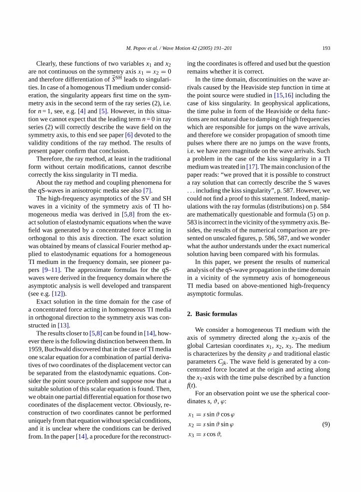
ting of SV and SH waves up toϑ = 60 because thedifference in velocities grows slower in the secondmodel of TI medium when angleϑ increases. Notethat in this case of TI medium the curvatures of

the slowness surfaces have the same sign at the kisspoints.

In order to estimate the contribution of the secondterms in Eqs.(12)and(13)we present them on graphs

F(

ig. 3. qS-wave field in second model of TI medium with wavelet(18). (a anc–f) Evolution of the wave field as angleϑ increases. For (c and d)ϑ = 0.50

d b) Graphs of the wavelet and modulus of its spectrum, respectively.; for (e and f)ϑ = 20.


Fig. 4. qS-wave field in second model of TI medium with wavelet(18). (a b)ϑ = 40; for (c and d)ϑ = 60. (e and f) The contributions of only second teof the displacement vector, respectively, forϑ = 60.

(e) and (f),Fig. 4, for the angleϑ = 60. By comparingthem with graphs (c) and (d) on the same figure, weconclude that they cannot be omitted without signifi-cant loss in accuracy.

4

achb qS-

–d) Evolution of the wave field as angleϑ increases. For (a andrms in Eqs.(12)and(13) to thex1-coordinate and to thex2-coordinate

. Conclusion

The numerical experiments prove that the approased on the high-frequency asymptotics of the


waves can be successfully used for describing the kisssingularity in TI media in the time domain. The corre-sponding formulas provide smooth transition the kisssingularity wave field to the ray formulas for SV andSH waves.

We observe that the displacement vector of the qS-wave field preserves essentially the direction of the ex-ternal force in a narrow vicinity of the symmetry axis.Precisely on the axis there is no distortion of the timepulse shape but with the increase of the distance to theaxis we observe distortion even when the splitting ofSV and SH waves is small.

Acknowledgements

One of the authors (M. Popov) is thankful to CNPq,grant no. 300603/94-0, and to the Russian Foundationfor Basic Research, grant no. 02-01-00260, for the fi-nancial support of this research.

References

[1] V.M. Babich, Ray method for the computation of the intensityof wave fronts in elastic inhomogeneous anisotropic medium,Problems Dyn. Theory Propagat. Seismic Waves 5 (1961)36–46, Leningrad University Press (in Russian) [Engl. Trans.:Geophys. J. Int. 118 (1994) 379–383].

[2] V.V. Kucherenko, Asymptotic behavior of solution of the systemA(x,−ih ∂

∂x

)u = 0 ash→ 0 in the case of characteristics of

4)

nti-Zap.Ingl.

ho-r ap-96)

[5] M.M. Popov, SH waves in a homogeneous transversely isotropicmedium generated by a concentrated force, Zap. Nauchn. Sem.POMI 264 (2000) 285–289 (in Russian) [Engl. Trans.: J. Math.Sci. 111 (5) (2002) 3791–3798].

[6] M.M. Popov, C. Camerlynck, Second term of the ray series andvalidity of the ray theory, J. Geophys. Res. 101 (1996) 817–826.

[7] C.H. Chapman, P.M. Shearer, Ray tracing in azimuthallyanisotropic media-II. Quasi-shear wave coupling, Geophys. J.Int. 96 (1989) 65–83.

[8] M.M. Popov, Asymptotics of the wave field in a vicinity ofthe axis of symmetry of a transversely isotropic homogeneousmedium, Zap. Nauchn. Semin. POMI 275 (2001) 199–211 (inRussian) [Engl. Trans.: J. Math. Sci. 117 (2) (2003) 4001–4007].

[9] M.J.P. Musgrave, Crystal Acoustics, Holden Day, San Fran-cisco, 1970.

[10] V.T. Buchwald, Elastic waves in anisotropic media, Proc. R.Soc. A. 252 (1959) 562–580.

[11] M.J. Lighthill, Studies on magneto-hydrodynamic waves andother anisotropic wave motions, Phil. Trans. R. Soc. A. 252(1960) 397–430.

[12] M.V. Fedoryuk, The method of Steepest Descent (in Russian),Nauka, Moscow, 1977.

[13] L.A. Molotkov, On an inner source in transversely isotropicmedium, Zap. Nauchn. Sem. POMI 264 (2000) 238–239 (inRussian) [Engl. Trans.: J. Math. Sci. 111 (5) (2002) 3763–3769].

[14] D. Gridin, Far-field asymptotics of the Green’s tensor for atransversely isotropic solid, Proc. R. Soc. Lond. A 456 (2000)571–591.

[15] A.G. Every, K.Y. Kim, Time domain dynamic response func-tions of elastically anisotropic solids, J. Acoust. Soc. Am. 95(1994) 2505–2516.

[16] V.A. Borovikov, D. Gridin, Kiss singularities of Green’s func-tions of non-strictly hyperbolic equations, Proc. R. Soc. Lond.

[ ty: a138

[ geo-

[ ely

[ rsely

variable multiplicity, Izv. AN SSSR, Ser. Mat. 58 (2) (197163–213 (in Russian).

[3] M.M. Popov, I.N. Shchitov, On the propagation of disconuities of a system of two interacting wave equations,Nauchn. Sem. POMI 264 (2000) 299–310 (in Russian) [Trans.: J. Math. Sci. 111 (5) (2002) 3799–3805].

[4] V. Vavrycuk, K. Yomogida, SH-waves Green tensor formogeneous transversely isotropic media by higher-ordeproximations in asymptotic ray theory, Wave Motion 23 (1983–93.

A. 457 (2001) 1059–1077.17] V. Vavrycuk, Properties of S waves near a kiss singulari

comparison of exact and ray solutions, Geophys. J. Int.(1999) 581–589.

18] M.M. Popov, Ray theory and Gaussian Beam method forphysicists, EDUFBA, Salvador, Bahia, 2002.

19] E.L. Faria, L. Stoffa, Finite-difference modeling in transversisotropic media, Geophysics 59 (2) (1994) 282–289.

20] R.G. Payton, Symmetry axis elastic waves for transveisotropic media, Q. Appl. Math. 35 (1977) 63–73.

qS-waves in a vicinity of the axis of symmetry of homogeneous transversely isotropic media

Documents

Transcript of qS-waves in a vicinity of the axis of symmetry of homogeneous transversely isotropic media