arX

iv:m

ath/

0308

173v

2 [

mat

h.A

G]

4 J

an 2

005

LECTURES ON MIRROR SYMMETRY, DERIVED CATEGORIES, AND

D-BRANES

ANTON KAPUSTIN AND DMITRI ORLOV

Abstract. This paper is an introduction to Homological Mirror Symmetry, derived cat-

egories, and topological D-branes aimed mainly at a mathematical audience. In the paper

we explain the physicists’ viewpoint of the Mirror Phenomenon, its relation to derived cat-

egories, and the reason why it is necessary to enlarge the Fukaya category with coisotropic

A-branes; we discuss how to extend the definition of Floer homology to such objects and

describe mirror symmetry for flat tori. The paper consists of four lectures which were given

at the Institute for Pure and Applied Mathematics (Los Angeles), March 2003, as part of

a program on Symplectic Geometry and Physics.

1. Mirror Symmetry From a Physical Viewpoint

The goal of the first lecture is to explain the physicists’ viewpoint of the Mirror Phe-

nomenon and its interpretation in mathematical terms proposed by Maxim Kontsevich in

his 1994 talk at the International Congress of Mathematicians [25]. Another approach to

Mirror Symmetry was proposed by A. Strominger, S-T. Yau, and E. Zaslow [41], but we

will not discuss it here.

From the physical point of view, Mirror Symmetry is a relation on the set of 2d confor-

mal field theories with N = 2 supersymmetry. A 2d conformal field theory is a rather

complicated algebraic object whose definition will be sketched in a moment. Thus Mirror

Symmetry originates in the realm of algebra. Geometry will appear later, when we spe-

cialize to a particular class of N = 2 superconformal field theories related to Calabi-Yau

manifolds.

Let us start with 2d conformal field theory. The data needed to specify a 2d CFT consist

of an infinite-dimensional vector space V (the space of states), three special elements in V

(the vacuum vector |vac〉, and two more elements L and L ), and a linear map Y from

V to the space of “formal fractional power series in z, z with coefficients in End(V ) ”

( Y is called the state-operator correspondence). The precise definition of what a “formal

fractional power series” means can be found in [19]; to keep things simple, one can pretend

that Y takes values in the space of Laurent series in z, z with coefficients in End(V ),

although such a definition is not sufficient for applications to Mirror Symmetry. These data

must satisfy a number of axioms whose precise form can be found in [19]. Roughly speaking,

they are

(i) Y (|vac〉) = idV .

The first author was supported in part by the DOE grant DE-FG03-92-ER40701. The second author

was supported in part by the grant of the President of RF for young scientists D-2731.2004.1, by Civic Re-

search Development Foundation (CRDF Award No RM1-2405-MO-02), and by the Russian Science Support

Foundation.

1

2

(ii) Y (L) =∑

n∈ZLn

zn+2 , Y (L) =∑

n∈ZLn

zn+2 for some Ln, Ln ∈ End(V ).

(iii) Both Ln and Ln satisfy the commutation relations of the Virasoro algebra, and

all Ln commute with all Lm.

(iv) [L−1, Y (v, z, z)] = ∂Y (v, z, z), [L0, Y (v, z, z)] = z∂Y (v, z, z) + Y (L0v, z, z), for

any v ∈ V, and similar conditions obtained by replacing Ln → Ln, ∂ → ∂.

(iv) Y (v)|vac〉 = ezL−1+zL−1v for any v ∈ V.(v) Y (v, z, z)Y (v′, z′, z′) has only power-like singularities on the diagonals z = z′ and

z = z′.

(vi) Y (v, z, z)Y (v′, z′, z′) − Y (v′, z′, z′)Y (v, z, z) is a formal distribution supported on

the diagonal.

Recall that the Virasoro algebra is an infinite-dimensional Lie algebra spanned by elements

Lm,m ∈ Z and the following commutation relations:

[Lm, Ln] = (m− n)Lm+n + cm3 −m

12δm,−n.

It is a unique central extension of the Witt algebra (the Lie algebra of vector fields on a

circle). The constant c is called the central charge. The Virasoro algebras spanned by Ln

and Ln are called right-moving and left-moving, respectively.

There are certain variations of this definition. The modification which we will need

most amounts to replacing all spaces and maps by their Z/2 -graded versions, and the

“commutativity” axiom (vi) with supercommutativity. From the physical viewpoint, this

means that we allow both fermions and bosons in our theory. Another important property

which must hold in any acceptable CFT is the existence of a non-degenerate bilinear form

on V which is compatible, in a suitable sense, with the rest of the data. Finally, most

CFTs of interest are “left-right symmetric.” This means that exchanging z and z, and

Ln and Ln, gives an isomorphic CFT. We will only consider left-right symmetric CFTs.

A more geometric approach to 2d CFT has been proposed by G. Segal [40]. In Segal’s

approach, one starts with a certain category whose objects are finite ordered sets of circles,

and morphisms are Riemann surfaces with oriented and analytically parametrized bound-

aries. Composition of morphisms is defined by sewing Riemann surfaces along boundaries

with compatible orientations. A 2d CFT is a projective functor from this category to the

category of Hilbert spaces which satisfies certain properties which are listed in [40, 10]. (A

projective functor from a category C to the category of Hilbert spaces is the same as a

functor from C to a category whose objects are Hilbert spaces, and morphisms are equiva-

lence classes of Hilbert space morphisms under the operation of multiplication by non-zero

scalars.) One can show that any 2d CFT in the sense of Segal’s definition gives rise to a 2d

CFT in the sense of our algebraic definition (see e.g. [10]). For example, the vector space

V which appears in our algebraic definition is the Hilbert space associated to a single circle

in Segal’s approach. The map Y comes from considering the morphism which corresponds

to a Riemann sphere with three holes. Conversely, it appears that any “algebraic” 2d CFT

which is left-right symmetric and is equipped with a compatible inner product gives rise to

a “geometric” 2d CFT in genus zero (i.e. with Riemann surfaces restricted to have genus

zero).

3

An N = 1 super-Virasoro algebra is a certain infinite-dimensional Lie super-algebra

which contains the ordinary Virasoro as a subalgebra. Apart from the Virasoro generators

Ln, n ∈ Z, it contains odd generators Qn, n ∈ Z. The additional commutation relations

read

[Lm, Qn] =(m

2− n

)Qm+n, [Qm, Qn] =

1

2Lm+n +

c

12m2δm,−n.

An N = 1 superconformal field theory (SCFT) is a 2d CFT with an action on V of two

copies of the N = 1 super-Virasoro algebra which is compatible with other structures of

the SCFT in a fairly obvious sense. 1

An N = 2 super-Virasoro algebra is a further generalization of the Virasoro algebra.

It is a certain infinite-dimensional Lie super-algebra which contains the N = 1 super-

Virasoro as a subalgebra. The even generators are Ln, Jn, n ∈ Z. The odd generators are

Q±n , n ∈ Z. The commutators read, schematically:

[L,L] ∼ L, [J, J ] ∼ central, [L, J ] ∼ J, [Q±, Q±] = 0,(1)

[L,Q±] ∼ Q±, [J,Q±] ∼ ±Q±, [Q±, Q∓] ∼ J + L+ central.(2)

The precise form of the commutation relations ca be found in [19]. The N = 1 super-

Virasoro subalgebra is spanned by Ln and Qn = Q+n +Q−

n . The relation between N = 1

and N = 2 super-Virasoro is analogous to the relation between the de Rham and Dolbeault

differentials on a complex manifold: Qn are analogous to d, while Q+n and Q−

n are

analogous to ∂ and ∂.

An N = 2 SCFT is an N = 1 SCFT with an action of two copies of N = 2 super-

Virasoro algebra which is compatible with the remaining structures of the SCFT. Thus we

have a hierarchy of algebraic structures:

Set of all CFTs ⊃ Set of all N = 1 SCFTs ⊃ Set of all N = 2 SCFTs

In fact, there is an even more general notion: 2d quantum field theory, without the adjective

“conformal.” We will not discuss it in these lectures.

It is possible to give a definition of N = 1 and N = 2 superconformal field theories a la

Segal. The role of Riemann surfaces is played by 2d supermanifolds equipped with N = 1

or N = 2 superconformal structure.

An isomorphism of (super-)conformal field theories is a 1-1 map V∼→ V ′ which preserves

all the relevant structures. Two N = 2 superconformal field theories can be isomorphic as

N = 1 superconformal field theories without being isomorphic as N = 2 superconformal

field theories. (When physicists say that two (super-)conformal field theories are “the same”,

they often neglect to specify which structures are preserved by the isomorphism; this is

usually clear from the context.)

N = 2 super-Virasoro algebra has an interesting automorphism called the mirror auto-

morphism:

M : Ln 7→ Ln, Jn 7→ −Jn, Q±n 7→ Q∓

n .

Suppose we have a pair of N = 2 superconformal field theories which are isomorphic

as N = 1 SCFTs. Let f : V∼→ V ′ be an isomorphism. We say that f is a (right)

mirror morphism of N = 2 CFTs if it acts as the identity on the “left-moving” N = 2

1Strictly speaking, we are talking about the Ramond-Ramond sector of the SCFT here.

4

super-Virasoro, and acts by the mirror automorphism on the “right-moving” N = 2 super-

Virasoro. This makes sense because the mirror automorphism acts as the identity on the

N = 1 super-Virasoro subalgebra of N = 2 super-Virasoro algebra. Exchanging left and

right, we get the notion of a left mirror morphism of N = 2 CFTs. Finally, if f acts as

the mirror automorphisms on both left and right super-Virasoro algebras, we will say that

f is a target-space complex conjugation.

By definition, two N = 2 SCFTs are mirror to each other if there is a (left or right)

mirror morphism between them. Clearly, if two N = 2 SCFTs are both (left-) mirror to a

third N = 2 SCFT, then the first two SCFTs are isomorphic (as N = 2 SCFTs). Thus the

mirror relation (for example, left) is an involutive relation on the set of isomorphism classes

of N = 2 SCFTs. We stress that if two N = 2 SCFTs are mirror to each other, then

they are isomorphic as N = 1 SCFTs, but usually not as N = 2 SCFTs. Many explicit

examples of mirror pairs of N = 2 SCFTs have been constructed in the physics literature;

one can construct more complicated examples by means of tensor product, orbifolding, etc.

Now let us turn to the relation between N = 2 SCFTs and Calabi-Yau manifolds. A

physicist’s Calabi-Yau is a compact complex manifold with a trivial canonical class equipped

with a Kahler class and a B-field (an element of H2(X,R)/H2(X,Z) ). It is believed that to

any physicist’s Calabi-Yau one can attach, in a natural way, an N = 2 SCFT which depends

on these geometric data. One can give the following heuristic argument supporting the claim.

First of all, to any physicist’s Calabi-Yau one can naturally attach a classical field theory

called the N = 2 sigma-model. Its Lagrangian is given by an explicit, although rather

complicated, formula (see e.g. [36]). Infinitesimal symmetries of this classical field theory

include two copies of N = 2 super-Virasoro algebra (with zero central charge). Second,

one can try to quantize this classical field theory while preserving N = 2 superconformal

invariance (up to an unavoidable central extension). The result of the quantization should

be an N = 2 SCFT.

Except for a few special cases, it is not known how to quantize the sigma-model exactly.

On the other hand, one has a perturbative quantization procedure which works when the

volume of the Calabi-Yau is large. That is, if one rescales the metric by a parameter t≫ 1,

gµν → t2gµν , and considers the limit t → ∞ (so called large volume limit), then one can

quantize the sigma-model order by order in 1/t expansion. It is believed that the resulting

power series in 1/t has a non-zero radius of convergence, and defines an actual N = 2

SCFT.

It is natural to ask if it is possible to reconstruct a Calabi-Yau starting from an N = 2

SCFT; as we will discuss shortly, the reconstruction problem does not have a unique answer.

However, some numerical characteristics of the “parent” Calabi-Yau X can be determined

rather easily. For example, the complex dimension of X is given by c/3, where c is the

central charge of the N = 2 super-Virasoro algebra. One can also determine the Hodge

numbers hp,q(X) in the following manner. Commutation relations of the N = 2 super-

Virasoro imply that the operator DB = Q+0 + Q+

0 on V squares to zero. DB is known as

a BRST operator (of type B, see below), and its cohomology is called the BRST cohomology.

The BRST cohomology Ker DB/ Im DB is finite-dimensional in any reasonable N = 2

5

SCFT. It is graded by the eigenvalues of the operators J0 and J0 known as left and right-

moving R-charges. The Hodge number hp,q(X) is simply the dimension of the component

with R-charges p− n2 and q − n

2 , where n = dimCX. This means, incidentally, that not

every N = 2 SCFT arises from a Calabi-Yau manifold: those which do, must have integral

n = c/3 and integral spectrum of J0 + n2 and J0 + n

2 in BRST cohomology. It is believed

that any N = 2 SCFT with integral c/3 and integral spectrum of J0 + n2 and J0 + n

2

is related to some Calabi-Yau manifold, if one allows certain kinds of singular Calabi-Yau

manifolds, such as orbifolds.

One can show that if two Calabi-Yau are complex-conjugate, then the corresponding

N = 2 SCFTs are related by target-space conjugation (in the sense explained above). This

explains why the name “target-space complex conjugation” was attached to a particular

kind of morphisms of N = 2 SCFTs. On the other hand, if two Calabi-Yau manifolds have

N = 2 SCFTs related by target-space complex conjugation, this does not imply that the

Calabi-Yau manifolds themselves are complex-conjugate; it merely implies that their N = 2

SCFTs are related in a simple way. Thus one obvious question is

Question 1. When do two Calabi-Yau manifolds produce isomorphic N = 2 SCFTs?

An answer to this question would interpret “quantum symmetries” of 2d SCFTs in geo-

metric terms. Another question of this kind is

Question 2. When do two Calabi-Yau manifolds produce N = 2 SCFTs which are mirror

to each other?

We say that two Calabi-Yau manifolds are related by mirror symmetry if the correspond-

ing N = 2 SCFTs are mirror.

First non-trivial examples of mirror pairs of Calabi-Yau manifolds have been constructed

by B. Greene and R. Plesser [14]. The simplest example in complex dimension three (this

dimension is the most interesting one from the physical viewpoint) is the following: one

of the Calabi-Yau manifolds is the Fermat quintic x5 + y5 + z5 + v5 + w5 = 0 in CP4,

while the other one is obtained by taking a quotient of the Fermat quintic by a certain

action of (Z/5)3 and blowing up the fixed points. We will not try to explain why these

two Calabi-Yau manifolds are mirror. (The original argument [14] relied on a conjectural

equivalence between the N = 2 SCFT corresponding to the Fermat quintic and a certain

integrable N = 2 SCFT constructed by D. Gepner. Later this issue has been studied in

detail by E. Witten [44] and now has the status of a physical “theorem.”)

The answer to the first question is highly non-trivial. This can be seen already in the

case when X is a complex torus with a flat metric (Lecture 2). For example, the torus

and its dual give the same N = 2 SCFT, even though they are usually not isomorphic as

complex manifolds. The answer to Question 2 – characterization of the mirror relation in

geometric terms – is the ultimate goal of the Mirror Symmetry program.

On the most basic level, a mirror relation between X and X ′ implies a relation between

their Hodge numbers hp,q(X) and hp,q(X ′). To see how this comes about, note that

along with the cohomology of DB = Q+0 + Q+

0 we may also consider the cohomology of

DA = Q−0 + Q+

0 . It can be shown that in any N = 2 SCFT satisfying the integrality

constraint these two cohomologies are isomorphic as bi-graded vector spaces [29]. Now

note that if X is mirror to X ′, then the cohomology of DA(X) in bi-degree (α, β) is

6

isomorphic to cohomology of DB(X ′) in bi-degree (−α, β). Recalling the relation between

the Hodge numbers of X and cohomology of DB(X), we infer an important relation

(3) hp,q(X) = hn−p,q(X ′).

If one plots the Hodge numbers of a complex manifold on a plane with coordinates p − qand p + q − n, the resulting table has the shape of a diamond (the Hodge diamond). For

any Calabi-Yau manifold the Hodge diamond is unchanged by a rotation by 180 degrees.

The relation (3) means that the Hodge diamonds of mirror Calabi-Yau manifolds are related

by a rotation by 90 degrees.

Of course, the existence of a mirror relation between X and X ′ implies much more than

this. The most promising approach to the problem of characterizing the mirror relation in

geometric terms has been proposed in 1994 by M. Kontsevich. In the remainder of this

lecture we will sketch Kontsevich’s proposal and its interpretation in physical terms.

A physicist’s Calabi-Yau has both a complex structure and a symplectic structure (the

Kahler form). One can gain a considerable insight into the Mirror Symmetry Phenomenon

by focusing one of the two structures. More precisely, if the B-field is present, we combine the

Kahler form ω and the (1, 1) part of the B-field into a “complexified Kahler form.” We will

regard the latter as parametrizing an “extended symplectic moduli space” of X. Similarly,

we regard the (0, 2) part of the B-field and the complex structure moduli as parametrizing

an “extended complex structure moduli space” of X. We would like to isolate some aspects

of the N = 2 SCFT which depend either only on the extended complex moduli, or only

on the extended symplectic moduli. The procedure for doing this was proposed by E.

Witten [45, 46] and is known as topological twisting.

Witten’s construction rests on the observation that many N = 2 SCFTs have finite-

dimensional sectors which are topological field theories, i.e. do not depend on the 2d metric

(the metric on the world-sheet, if we use string theory terminology.) In fact, for many

N = 2 SCFTs there are two such sub-theories ; they are known as A- and B-models.

N = 2 SCFTs related to Calabi-Yau manifolds belong precisely to this class of theories.

Let us recall some basic facts about 2d topological field theories. These theories are

similar to, but much simpler than, 2d CFTs. They can be described by axioms similar

to Segal’s axioms [2]. One starts with a category whose objects are finite ordered sets

of oriented and parametrized circles and morphisms are oriented 2d manifolds (without

complex structure) bounding the circles. A 2d topological field theory is a functor from this

category to the category of finite-dimensional (graded) vector spaces which satisfies certain

requirements similar to Segal’s. As for 2d CFTs, there is a purely algebraic reformulation of

this definition. It turns out that the “topological” counterpart of the notion of a conformal

field theory is the well-known notion of a super-commutative Frobenius algebra, i.e. a

super-commutative algebra with an invariant metric (see e.g. [6]).

A detailed discussion of Witten’s procedure for constructing a 2d TFT out of an N = 2

SCFT is beyond the scope of these lectures. Roughly speaking, one passes from the space V

to its BRST cohomology. One can show that the state-operator correspondence Y descends

to a super-commutative algebra structure on the BRST cohomology. The invariant metric

on BRST cohomology comes from a metric on V.

7

Note that we have two essentially different choices of a BRST operator: DA or DB.

(One can also consider D′A = Q+

0 + Q−0 and D′

B = Q−0 + Q−

0 , but these can be trivially

related to DA and DB by replacing X with its complex-conjugate.) Thus Witten’s

construction associates to any physicist’s Calabi-Yau X two topological field theories,

called the A-model and the B-model, respectively.

It turns out that the A-model does not change as one varies the extended complex struc-

ture moduli, while the B-model does not depend on the extended symplectic moduli. In

other words, the A-model isolates the symplectic aspects of the Calabi-Yau, while the B-

models isolates the complex ones. In fact, the state space of the A-model is naturally

isomorphic to the de Rham cohomology H∗,∗(X), while the state space of the B-model is

naturally isomorphic to the Dolbeault cohomology

H∗(Λ∗T 1,0X),

where T 1,0X is the holomorphic tangent bundle of X. For a Calabi-Yau manifold,

Hq(ΛpT 1,0X) is isomorphic to Hn−p,q(X), but not canonically: the isomorphism depends

on the choice of a holomorphic section of the canonical line bundle. Note also that the spaces

of the A and B-models are bi-graded. From the physical point of view, the bi-grading comes

from the decomposition of the state spaces into the eigenspaces of J0 and J0.

The algebra structure in the B-case is the obvious one, while in the A-case it is a deforma-

tion of the obvious one which depends on the extended symplectic structure on X ; H∗(X)

equipped with this deformed algebra structure is known as the quantum cohomology ring

of X.

Mirror symmetry acts on A and B-models in a very simple way. It is easy to see that the

mirror automorphism exchanges DA and DB . Thus if X and X ′ are a mirror pair of

physicist’s Calabi-Yau manifolds, then the A-model of X is isomorphic to the B-model of

X ′, and vice versa. We will say that X and X ′ are weakly mirror if the A-model of X is

isomorphic to the B-model of X ′, and vice-versa. The notion of weak mirror symmetry is

easier to work with, since one can define A and B-models of a Calabi-Yau directly, without

appealing to the ill-defined quantization of the sigma-model. But clearly a lot of information

is lost in the course of topological twisting, and one would like to find some richer objects

associated to an N = 2 SCFT.

M. Kontsevich proposed that a suitable enriched version of the B-model is the bounded

derived category of coherent sheaves on X, which we will denote Db(X), while the en-

riched version of the A-model is some version of the derived Fukaya category of X, which

will be denoted DF0(X). In other words, he conjectured that if X and X ′ are mirror,

then Db(X) is equivalent to DF0(X′) and vice versa. This is known as the Homologi-

cal Mirror Conjecture (HMC). If the converse statement were true, this would completely

answer Question 1 and 2.

Let us sketch the definitions of these two categories. Let X be a smooth complex

manifold. An object of the bounded derived category on X is a bounded complex of

holomorphic vector bundles on X, i.e. a finite sequence of holomorphic vector bundles and

morphisms between them

0→ · · · → En−1 → En → En+1 → · · · → 0,

8

so that the composition of any two successive morphisms is zero. We remind the reader

that the cohomology of such a complex is a sequence of coherent sheaves on X. To define

morphisms in the derived category, we first consider the category of bounded complexes

Cb(X), where morphisms are defined as chain maps between complexes. A morphism in

this category is called a quasi-isomorphism if it induces an isomorphism on the cohomology

of complexes. The idea of the derived category is to identify all quasi-isomorphic complexes.

That is, the bounded derived category Db(X) is obtained from Cb(X) by formally invert-

ing all quasi-isomorphisms. In this definition, one can replace holomorphic vector bundles

by arbitrary coherent sheaves; the resulting derived category is unchanged. Lecture 3 will

discuss derived categories in more detail.

While coherent sheaves and their complexes are very familiar creatures and are the basic

tool of algebraic geometry, the derived Fukaya category DF0(X) is a much more recent

invention. It is obtained by a rather complicated algebraic procedure from a certain geomet-

rically defined category called the Fukaya category F(X). The latter has been introduced

by K. Fukaya in [8]. Actually, F(X) is not quite a category: there are additional struc-

tures on morphisms (multiple compositions and the differential), and the composition of

morphisms is associative only up to a chain homotopy. Such a structure is called an A∞

category. The Fukaya category depends only on the extended symplectic structure on X.

Objects of the Fukaya category are, roughly speaking, triples (Y,E,∇), where Y is a

Lagrangian submanifold of X, E is a complex vector bundle on Y with a Hermitian

metric, and ∇ is a flat unitary connection on E. This definition is only approximate, for

several reasons. First of all, not every Lagrangian submanifold Y is allowed: the so-called

Maslov class of Y must vanish (the Maslov class is a class in H1(Y,Z) ). Second, Y

has to be a graded Lagrangian submanifold (this notion was defined in 1968 by J. Leray

for the case of Lagrangian submanifolds in a symplectic vector space, and generalized by

Kontsevich to the Calabi-Yau case). Third, it is not completely clear if the flat connection

∇ has to be unitary. There are some indications that it might be necessary to relax this

condition and require instead the eigenvalues of the monodromy representation to have unit

absolute value. Fourth, in the presence of the B-field ∇ must be projectively flat rather

than flat [19].

The space of morphisms in the Fukaya category is defined by means of the Floer complex.

This will be discussed in Lecture 2.

The relation between the Homological Mirror Conjecture and the A and B-models is the

following [25]. Given a triangulated category (more precisely, an “enhanced triangulated

category” [3]), one can study its deformations. Information about deformations is encoded

in the Hochschild cohomology of the category in question. In the case of the derived category

of coherent sheaves, Hochschild cohomology seems to coincide with the cohomology of the

exterior algebra of the holomorphic tangent bundle, i.e. the state space of the B-model.2

Kontsevich conjectured that the Hochschild cohomology of the derived Fukaya category is

the quantum cohomology ring of X, i.e. the state space of the A-model [25]. Thus the

equivalence of Db(X) and DF0(X′) is likely to imply that the B-model of X is isomorphic

2We say “seems”, because there is no complete proof of this yet.

9

(as a 2d TFT) to the A-model of X ′. In other words, Homological Mirror Symmetry seems

to imply weak mirror symmetry.

Homological Mirror Symmetry Conjecture also has a clear physical meaning. The physical

idea is to generalize the notion of a 2d TFT to allow the 2d world-sheet to have boundaries

(see e.g. [47]). This generalization also makes sense in the full N = 2 SCFT and leads to

the notion of a D-brane, which plays a very important role in string theory [37]. A D-brane

is a nice boundary condition for the SCFT. It is not completely clear what this means in

the quantum case, so let us discuss this notion using classical field theory. A classical 2d

field theory is defined by an action which is an integral of a local Lagrangian over the 2d

world-sheet. So far we took the world-sheet to be a cylinder whose noncompact direction

was parametrized by the “time” variable. Thus the space was topologically a circle. Now

let us take the space to be an interval I. The world-sheet becomes R × I. In order for

the classical field theory to be well-defined, we require the the Cauchy problem for the

Euler-Lagrange equations to have a unique solution, at least locally. This requires imposing

a suitable boundary condition on the fields and their derivatives on the boundary of the

world-sheet. For example, one can impose Dirichlet boundary conditions (i.e. vanishing) on

some scalar fields which appear in the Lagrangian.3 A classical D-brane is simply a choice

of such a boundary condition.

If the classical field theory has some symmetries, it is reasonable to require the boundary

condition to preserve this symmetry. For example, N = 1 sigma-models have two copies

of N = 1 super-Virasoro algebra as their symmetries. It is not possible to preserve both

of them, but there exist many boundary conditions which preserve the diagonal subalgebra.

Such boundary conditions are ordinary D-branes of superstring theory [37]. In the N = 2

case, we have two copies of N = 2 super-Virasoro, and we may require the boundary

condition to preserve the diagonal N = 2 super-Virasoro. Such boundary conditions are

called D-branes of type B, or simply B-branes, because they are related to the B-model (see

below). One can also exploit the existence of the mirror automorphism M and consider

boundary conditions which preserve a different N = 2 super-Virasoro subalgebra, namely

the one spanned by

Ln + Ln, −Jn + Jn, Q−n + Q+

n , Q+n + Q−

n , n ∈ Z.

The corresponding branes are called D-branes of type A, or simply A-branes.

Given a classical D-brane, we can try to quantize a classical field theory on R× I with

boundaries, which related to this D -brane, so that the quantized theory has one copy

of N = 2 super-Virasoro as its symmetry algebra. If such a quantization is possible, we

say that the classical D-brane is quantizable, and the classical D-brane together with its

quantization will be called a quantum D-brane. This is not a very satisfactory way to define

quantum D-branes, and it remains an interesting problem to find a satisfactory and fully

quantum definition of a boundary condition for a 2d SCFT.

Now let us turn to the relation of A and B-branes with A and B-models. A and B-

models are obtained from the N = 2 SCFT by topological twisting. Roughly speaking,

twisting amounts to truncating the theory to the cohomology of DA or DB . Now note

3The letter D in the word “D-brane” actually came from “Dirichlet.”

10

that DA (resp. DB ) sits in the N = 2 super-Virasoro which is preserved by the A-type

(resp. B-type) boundary condition. The significance of this is that the A-twist is consistent

with A-type boundary conditions, while the B-twist is consistent with B-type boundary

conditions. Thus an A-brane (resp. B-brane) gives rise to a consistent boundary condition

for the A-model (resp. B-model).4

One can show that the set of A-branes (or B-branes) has the structure of a category. The

space of morphisms between two branes A and A′ is simply the space of states of the

2d TFT on R × I, with boundary conditions on the two ends corresponding to A and

A′. Equivalently, one considers the state space of the N = 2 SCFT on an interval, and

computes its BRST cohomology with respect to DA. The composition of morphisms can

be defined with the help of the state-operator correspondence Y (or rather, its analogue

in the case of a 2d SCFT with boundaries).

To summarize, to any physicist’s Calabi-Yau we can attach two categories: the categories

of A-branes and B-branes. One can argue that the category of A-branes (resp. B-branes)

does not depend on the extended complex (resp. extended symplectic) moduli [47]. One can

think of these categories as the enriched versions of the A and B-models: while the A-model

is a TFT on a world-sheet without boundaries, the totality of A-branes corresponds to the

same 2d TFT on a world-sheet with boundaries and with all possible boundary conditions.

Further, it is obvious that if two Calabi-Yau manifolds are related by a mirror morphism,

then the A-brane category of the first manifold is equivalent to the B-brane category of

the second one, and vice versa. Obviously, if two N = 2 SCFTs related two Calabi-Yau

manifolds are isomorphic, then the corresponding categories of A-branes (and B-branes) are

simply equivalent.

The Homological Mirror Conjecture would follow if we could prove that the category of

A-branes (resp. B-branes) is equivalent to DF0(X) (resp. Db(X) ). Alas, we cannot

hope to prove this, because we do not have an honest definition of a D-brane. What we do

know is that holomorphic vector bundles are examples of B-branes, and objects of the Fukaya

category are examples of A-branes [47]. Furthermore, Witten showed that in this special case

morphisms in the category of B-branes and A-branes agree with morphisms in the categories

Db(X) and DF0(X), respectively [47]. This computation served as a motivation for

Kontsevich’s conjecture. More recently it was shown that more general coherent sheaves,

as well as complexes of coherent sheaves, are also valid B-branes. On the other hand, it has

been shown recently that the Fukaya category is only a full subcategory of the category of

A-branes, that is, for some X there exist A-branes which are not isomorphic to any object

of DF0(X) [20]. This means that the symplectic side of Kontsevich’s conjecture needs

substantial modification. This will be discussed in more detail in Lecture 4.

From the mathematical point of view, the Homological Mirror Conjecture is not well-

defined, because it is not clear how to quantize the sigma-model for an arbitrary Calabi-Yau

manifold. But there is a class of Calabi-Yaus for which the sigma-model can be quantized,

and the corresponding N = 2 SCFTs can be described quite explicitly. These are complex

tori with a flat Kahler metric and arbitrary B-field. One can easily determine which pairs

4Axioms for boundary conditions in 2d TFTs have been discussed by G. Moore and G. Segal [31] and

C.I. Lazaroiu [27].

11

of such Calabi-Yaus give mirror N = 2 SCFTs; the resulting criterion can be expressed

in terms of linear algebra [19]. (This will be discussed in Lecture 2). Thus in the case

of flat tori the Homological Mirror Conjecture is mathematically well-defined (modulo the

issues related to the precise definition of the Fukaya category). In [39] A. Polishchuk and

E. Zaslow proved it for tori of real dimension two. But there are strong arguments showing

that for higher-dimensional tori the Homological Mirror Conjecture cannot hold, unless one

substantially enlarges the Fukaya category by adding new objects. This will be discussed in

Lecture 4.

For more general Calabi-Yaus, one can take the Homological Mirror Conjecture as an

attempt to give a mathematical definition of the mirror relation. Then the main issues

are the precise definition of the Fukaya category, and the verification that the numerous

mirror pairs proposed by physicists and mathematicians are in fact mirror in the sense of

the Homological Mirror Conjecture.

Another approach to mirror symmetry has been proposed in [41] and is known as the SYZ

Conjecture. According to this conjecture, mirror Calabi-Yau manifolds admit fibrations by

special Lagrangian tori which in some sense are “dual” to each other. Recently a relation

between the Homological Mirror Conjecture and the SYZ Conjecture has been studied in

the paper [26].

2. Mirror Symmetry for Flat Complex Tori

In this lecture we describe N = 2 superconformal field theories (SCFT) related to

complex tori T endowed with a flat Kahler metric G and a constant 2-form B (the

B-field). We will give a criterion when two such data (T,G,B) and (T ′, G′, B′) produce

isomorphic N = 2 SCFT and when they produce N = 2 SCFT which are mirror to each

other.

As explained in Lecture 1, to define an N = 2 superconformal field theory we need

to specify an infinite-dimensional Z2 -graded vector space of states V, a vacuum vec-

tor |vac〉, a state-operator correspondence Y from V to the space of “formal fraction

power series in z, z with coefficients in End(V ) ” and, finally, the super-Virasoro elements

L, L,Q±, Q±, J, J which enter into the definition of the superconformal structure (see Lec-

ture 1).

We start with some notations. Let Γ ∼= Z2d be a lattice in a real vector space U of

dimension 2d, and let Γ∗ ⊂ U∗ be the dual lattice. Consider real tori T = U/Γ, T ∗ =

U∗/Γ∗. Let G be a metric on U, i.e. a positive symmetric bilinear form on U, and

let B be a real skew-symmetric bilinear form on U. Denote by l the natural pairing

Γ × Γ∗ → Z. (The natural pairing U × U∗ → R will be also denoted as l. ) Choose

generators e1, . . . , e2d ∈ Γ. The components of an element w ∈ Γ in this basis will be

denoted by wi, i = 1, . . . , 2d. The components of an element m ∈ Γ∗ in the dual basis will

be denoted by mi, i = 1, . . . , 2d. We also denote by Gij , Bij the components of G, B in

this basis. It will be apparent that the superconformal field theory which we construct does

not depend on the choice of basis in Γ. In the physics literature Γ is sometimes referred

to as the winding lattice, while Γ∗ is called the momentum lattice.

12

Consider a triple (T,G,B). With any such triple we associate an N = 2 superconformal

field theory V which may be regarded as a quantization of the supersymmetric sigma-model.

The state space of the SCFT V is

V = Hb ⊗C Hf ⊗C C [Γ⊕ Γ∗].

Here Hb and Hf are bosonic and fermionic Fock spaces defined below, while C [Γ⊕ Γ∗]

is the space of the group algebra of Γ⊕ Γ∗ over C.

To define Hb, consider an algebra over C with generators αis, α

is, i = 1, . . . , 2d, s ∈ Z\0

and relations

(4) [αis, α

jp] = s

(G−1

)ijδs,−p, [αi

s, αjp] = s

(G−1

)ijδs,−p, [αi

s, αjp] = 0.

If s is a positive integer, αi−s and αi

−s are called left and right bosonic creators, re-

spectively, otherwise they are called left and right bosonic annihilators. Either creators or

annihilators are referred to as oscillators.

The space Hb is defined as the space of polynomials of even variables ai−s, a

i−s, i =

1, . . . , 2d, s = 1, 2, . . . . The bosonic oscillator algebra acts on the space Hb via

αi−s 7→ ai

−s·, αi−s 7→ ai

−s·,αi

s 7→ s(G−1

)ij ∂

∂aj−s

, αis 7→ s

(G−1

)ij ∂

∂aj−s

,

for all positive s. This is the Fock-Bargmann representation of the bosonic oscillator al-

gebra. The vector 1 ∈ Hb is annihilated by all bosonic annihilators and will be denoted

|vacb〉.The space Hb will be regarded as a Z2 -graded vector space with a trivial (purely even)

grading. It is clear that Hb can be decomposed as Hb ⊗ Hb, where Hb (resp. Hb ) is the

bosonic Fock space defined using only the left (right) bosonic oscillators.

To define Hf , consider an algebra over C with generators ψis, ψ

is, i = 1, . . . , 2d, s ∈ Z+ 1

2

subject to relations

(5) ψis, ψ

jp =

(G−1

)ijδs,−p, ψi

s, ψjp =

(G−1

)ijδs,−p, ψi

s, ψjp = 0.

If s is positive, ψi−s and ψi

−s are called left and right fermionic creators respectively,

otherwise they are called left and right fermionic annihilators. Collectively they are referred

to as fermionic oscillators.

The space Hf is defined as the space of skew-polynomials of odd variables θi−s, θ

i−s, i =

1, . . . , 2d, s = 1/2, 3/2, . . . . The fermionic oscillator algebra (5) acts on Hf via

ψi−s 7→ θi

−s·, ψi−s 7→ θi

−s·,ψi

s 7→(G−1

)ij ∂

∂θj−s

, ψis 7→

(G−1

)ij ∂

∂θj−s

,

for all positive s ∈ Z + 12 . This is the Fock-Bargmann representation of the fermionic

oscillator algebra. The vector 1 ∈ Hf is annihilated by all fermionic annihilators and will

be denoted |vacf 〉. The fermionic Fock space has a natural Z2 grading such that |vacf 〉is even. It can be decomposed as Hf ⊗ Hf , where Hf (resp. Hf ) is constructed using

only the left (right) fermionic oscillators.

13

For w ∈ Γ, m ∈ Γ∗ we will denote the vector w ⊕m ∈ C [Γ⊕ Γ∗] by (w,m). We will

also use a shorthand |vac,w,m〉 for

|vacb〉 ⊗ |vacf 〉 ⊗ (w,m).

To define V, we have to specify the vacuum vector, T, T , and the state-operator corre-

spondence Y. But first we need to define some auxiliary objects. We define the operators

W : V → V ⊗ Γ and M : V → V ⊗ Γ∗ as follows:

W i : b⊗ f ⊗ (w,m) 7→ wi(b⊗ f ⊗ (w,m)), Mi : b⊗ f ⊗ (w,m) 7→ mi(b⊗ f ⊗ (w,m)).

We also set

∂Xj(z) =1

z

(G−1

)jkPk +

∞∑′

s=−∞

αjs

zs+1, ∂Xj(z) =

1

z

(G−1

)jkPk +

∞∑′

s=−∞

αjs

zs+1,

ψj(z) =∑

r∈Z+ 1

2

ψjr

zr+1/2, ψj(z) =

∑

r∈Z+ 1

2

ψjr

zr+1/2,

where a prime on a sum over s means that the term with s = 0 is omitted, and Pk and

Pk are defined by

Pk =1√2(Mk + (−Bkj −Gkj)W

j), Pk =1√2(Mk + (−Bkj +Gkj)W

j).

Note that we did not define Xj(z, z) themselves, but only their derivatives. The reason

is that the would-be field Xj(z, z) contains terms proportional to log z and log z, and

therefore is not a “fractional power series.”

The vacuum vector of V is defined by

|vac〉 = |vac, 0, 0〉.

The general formula for the state-operator correspondence Y is complicated and can be

found in [19]. We will only list a few special cases of the state-operator correspondence.

The states αj−s|vac, 0, 0〉 and αj

−s|vac, 0, 0〉 are mapped by Y to

1

(s− 1)!∂sXj(z),

1

(s − 1)!∂sXj(z).

The states ψj−s|vac, 0, 0〉 and ψj

−s|vac, 0, 0〉 are mapped to

1

(s− 12)!∂s−1/2ψj(z),

1

(s − 12 )!∂s−1/2ψj(z).

To define an N = 2 superconformal structure on V, we need to choose a complex

structure I on U with respect to which G is a Kahler metric. Let ω = GI be the

corresponding Kahler form. Then the left-moving vectors are defined as follows:

L =1

2G (a−1, a−1)−

1

2G(θ−1/2, θ−3/2

),

Q± =−i

4√

2(G∓ iω)

(θ−1/2, a−1

),

J = − i2ω(θ−1/2, θ−1/2

).

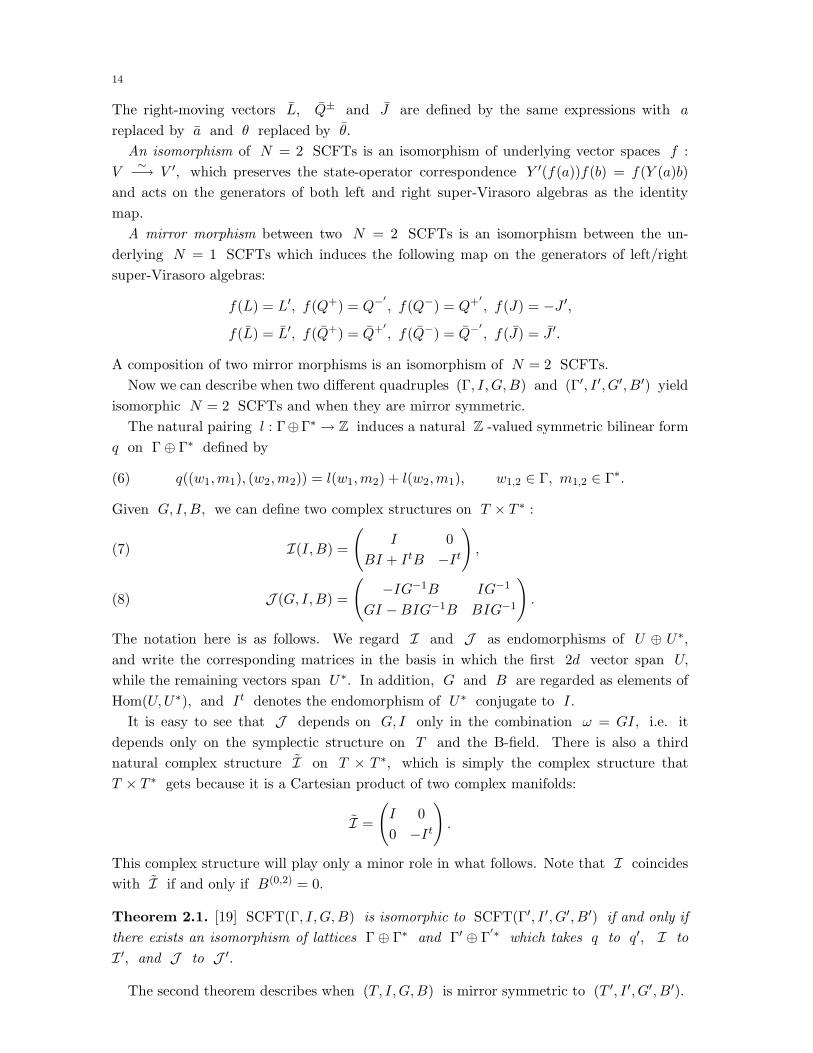
14

The right-moving vectors L, Q± and J are defined by the same expressions with a

replaced by a and θ replaced by θ.

An isomorphism of N = 2 SCFTs is an isomorphism of underlying vector spaces f :

V∼−→ V ′, which preserves the state-operator correspondence Y ′(f(a))f(b) = f(Y (a)b)

and acts on the generators of both left and right super-Virasoro algebras as the identity

map.

A mirror morphism between two N = 2 SCFTs is an isomorphism between the un-

derlying N = 1 SCFTs which induces the following map on the generators of left/right

super-Virasoro algebras:

f(L) = L′, f(Q+) = Q−′

, f(Q−) = Q+′

, f(J) = −J ′,

f(L) = L′, f(Q+) = Q+′

, f(Q−) = Q−′

, f(J) = J ′.

A composition of two mirror morphisms is an isomorphism of N = 2 SCFTs.

Now we can describe when two different quadruples (Γ, I,G,B) and (Γ′, I ′, G′, B′) yield

isomorphic N = 2 SCFTs and when they are mirror symmetric.

The natural pairing l : Γ⊕Γ∗ → Z induces a natural Z -valued symmetric bilinear form

q on Γ⊕ Γ∗ defined by

(6) q((w1,m1), (w2,m2)) = l(w1,m2) + l(w2,m1), w1,2 ∈ Γ, m1,2 ∈ Γ∗.

Given G, I,B, we can define two complex structures on T × T ∗ :

I(I,B) =

(I 0

BI + ItB −It

),(7)

J (G, I,B) =

(−IG−1B IG−1

GI −BIG−1B BIG−1

).(8)

The notation here is as follows. We regard I and J as endomorphisms of U ⊕ U∗,

and write the corresponding matrices in the basis in which the first 2d vector span U,

while the remaining vectors span U∗. In addition, G and B are regarded as elements of

Hom(U,U∗), and It denotes the endomorphism of U∗ conjugate to I.

It is easy to see that J depends on G, I only in the combination ω = GI, i.e. it

depends only on the symplectic structure on T and the B-field. There is also a third

natural complex structure I on T × T ∗, which is simply the complex structure that

T × T ∗ gets because it is a Cartesian product of two complex manifolds:

I =

(I 0

0 −It

).

This complex structure will play only a minor role in what follows. Note that I coincides

with I if and only if B(0,2) = 0.

Theorem 2.1. [19] SCFT(Γ, I,G,B) is isomorphic to SCFT(Γ′, I ′, G′, B′) if and only if

there exists an isomorphism of lattices Γ⊕ Γ∗ and Γ′ ⊕ Γ′∗ which takes q to q′, I to

I ′, and J to J ′.

The second theorem describes when (T, I,G,B) is mirror symmetric to (T ′, I ′, G′, B′).

15

Theorem 2.2. [19] SCFT(Γ, I,G,B) is mirror to SCFT(Γ′, I ′, G′, B′) if and only if there

is an isomorphism of lattices Γ⊕ Γ∗ and Γ′ ⊕ Γ′∗ which takes q to q′, I to J ′, and

J to I ′.

This theorem allows to give many examples of mirror pairs of tori. Suppose that we are

given a complex torus (T, I) with a constant Kahler form ω, and suppose that T = A×B,where A and B are Lagrangian sub-tori with respect to ω. In particular, the lattice Γ

decomposes as ΓA ⊕ ΓB . Let A be the dual torus for A, and let T ′ = A × B. The

lattice corresponding to T ′ is Γ′ = Γ∗A ⊕ ΓB , and there is an obvious isomorphism from

Γ⊕Γ∗ to Γ′⊕Γ′∗ which takes q to q′. We let I ′ and J ′ to be the image of J and I,

respectively, and invert the relationship between I ′,J ′ and I ′, ω′, B′ to find the complex

structure, the symplectic form, and the B-field on T ′. It is easy to check that this procedure

always produces a complex torus with a flat Kahler metric and a B-field which is mirror to

the original one. This recipe is a special case of the physical notion of T-duality [36].

We will soon see how these results can be used to test the Homological Mirror Conjecture

for flat tori. First, let us recall the formulation of the conjecture.

A physicist’s Calabi-Yau (X,G,B) is both a complex manifold and a symplectic man-

ifold (the symplectic form being the Kahler form ω = GI ). We can associate to each

such manifold a pair of triangulated categories: the bounded derived category of coherent

sheaves Db(X) and the derived Fukaya category DF0(X). The former depends only on

the complex structure of X, while the latter depends only on its symplectic structure. The

Homological Mirror Conjecture (HMC) asserts that if two algebraic Calabi-Yaus (X,G,B)

and (X ′, G′, B′) are mirror to each other, then Db(X) is equivalent to DF0(X′), and

vice versa Db(X ′) is equivalent to DF0(X).

Next, we need to recall the definitions of these two categories. We begin with the Fukaya

category F(X). An object of the Fukaya category is a triple (Y,E,∇E) where Y is a

graded Lagrangian submanifold of X, E is a complex vector bundle on Y with a Her-

mitian metric, and ∇E is a flat unitary connection of E. The only term which needs

to be explained here is “graded Lagrangian submanifold.” This notion was introduced by

J. Leray in 1968 in the case of Lagrangian submanifolds in a symplectic affine space, and

generalized by Kontsevich to the Calabi-Yau case in [25]. Let us first recall the definition of

the Maslov class of a Lagrangian submanifold. Let us choose a holomorphic section Ω of

the canonical line bundle (which is trivial for Calabi-Yaus). Restricting it to Y, we obtain

a nowhere vanishing n -form. On the other hand, we also have a volume form vol on

Y, which comes from the Kahler metric on X. This is also a nowhere vanishing n -form

on Y, and therefore Ω|Y = h · vol, where h is a nowhere vanishing complex function

on Y. The function h can be thought of as an element of H0(Y, C∞∗Y ), where C∞∗

Y is

the sheaf of C∗ -valued infinitely smooth functions on Y. The standard exponential exact

sequence gives a homomorphism from H0(Y, C∞∗Y ) to H1(Y,Z), and the Maslov class of

Y is defined as the image of h under this homomorphism. (Explicitly, the Cech cocycle

representing the Maslov class is constructed as follows: choose a good cover of Y, take the

logarithm of h on each set of the cover, divide by 2πi, and compare the results on double

overlaps). Although the definition of the Maslov class seems to depend both on the complex

16

and symplectic structures on X, in fact it is independent of the choice of complex struc-

ture. Note also that if the Maslov class vanishes, the logarithm of h exists as a function,

and is unique up to addition of 2πim,m ∈ Z. A graded Lagrangian submanifold Y is a

Lagrangian submanifold in X with a vanishing Maslov class and a choice of the branch of

log h.

Morphisms are defined as follows. Suppose we are given two objects (Y1, E1,∇1) and

(Y2, E2,∇2). We will assume that Y1 and Y2 intersect transversally at a finite number

of points; if this is not the case, we should deform one of the objects by flowing along a

Hamiltonian vector field, until the transversality condition is satisfied. Let ei, i ∈ I be

the set of intersection points of Y1 and Y2. Now we consider the Floer complex. As a

vector space, it is a direct sum of vector spaces

Vi = Hom(E1(ei), E2(ei)), i ∈ I.

The grading is defined as follows. At any point p ∈ Y the space TpY defines a point q

in the Grassmannian of Lagrangian subspaces in the space TpX. Let us denote by Lagp

the universal cover of the Lagrangian Grassmannian of the space TpX. On a Calabi-Yau

variety X, this spaces fit into a fiber bundle over X denoted by Lag [25]. Grading of

Y provides a canonical lift of q to Lagp for all p ; this lifts assemble into a section of

the restriction of Lag to Y [25]. Thus for each intersection point ei we have a pair of

points q1, q2 ∈ Lagei. The grade of the component of the Floer complex corresponding to

ei is the Maslov index of q1, q2 (see [4] for a definition of the Maslov index.) Finally, we

need to define the differential. Let ei and ej be a pair of points whose grade differs by

one. The component of the Floer differential which maps Vi to Vj is defined by counting

holomorphic disks in X with two marked points on the boundary, so that the two marked

points are ei and ej (the Maslov index of ej is the Maslov index of ei plus one), and the

two intervals which make up the boundary of the disks are mapped to Y1 and Y2. Note

that in order to compute the differential one has to choose an (almost) complex structure

J on X such that the form ω(·, J ·) is a Hermitian form on the tangent bundle of X.

For a precise definition of the Floer differential, see [9]. The space of morphisms in the

Fukaya category is defined to be the Floer complex. The composition of morphisms can be

defined using holomorphic disks with three marked points and boundaries lying on three

Lagrangian submanifolds.

The definition sketched above is only approximate. First, in order to define the Floer

differential one has to fix a relative spin structure on Y [9]. Second, the Floer differential

does not square to zero in general, so the Floer “complex” is not really a complex. A related

difficulty is that the composition of morphisms is associative only up to homotopy, which

depends on certain ternary product of morphisms. Actually, there is an infinite sequence

of higher products in the Fukaya category, which are believed to satisfy the identities of an

A∞ category (see [24] for a review of A∞ categories). It is also believed that changing

the almost complex structure J gives an equivalent A∞ category, so that the equivalence

class of the Fukaya category is a symplectic invariant. For a detailed discussion of these

issues see [9].

17

If the B-field is non-zero, one has to modify the definition of the Fukaya category as

follows. Objects are triples (Y,E,∇E), where Y is a graded Lagrangian submanifold, E

is a vector bundle on Y with a Hermitian metric, and ∇E is a Hermitian connection on

E such that its curvature satisfies

∇2E = 2πiB|Y .

Thus the connection is projectively flat rather than flat.

Morphisms are modified in the following way: all occurrences of the symplectic form ω

in the definition of the Floer complex and higher products are replaced with ω + iB. The

modified Fukaya category of a symplectic manifold X with a B-field B will be denoted

F(X,B).

The Fukaya category F(X,B) is not a true category, but an A∞ category with a

translation functor. The set of morphisms between two objects in an A∞ –category is a

differential graded vector space. To any A∞ –category one can associate a true category

which has the same objects but the space of morphisms between two objects is the 0–th

cohomology group of the morphisms in the A∞ –category. Applying this construction to

F(X,B), we obtain a true category F0(X,B) which is also called the Fukaya category.

Considering twisted complexes over F(X,B) M.Kontsevich [25] also constructs a certain

triangulated category DF0(X,B). We will call it the derived Fukaya category. The category

DF0(X,B) contains F0(X,B) as a full subcategory.

In the next lecture we will discuss the derived category of coherent sheaves, and use its

properties to test the Homological Mirror Conjecture.

3. Derived Categories of Coherent Sheaves and a Test of the Homological

Mirror Conjecture

Let X be a complex algebraic variety (or a complex manifold). Denote by OX the sheaf

of regular functions (or the sheaf of holomorphic functions). Recall that a coherent sheaf

is a sheaf of OX –modules that locally can be represented as a cokernel of a morphism of

algebraic (holomorphic) vector bundles. Coherent sheaves form an abelian category which

will be denoted by coh(X).

Next we recall the definition of a derived category and describe some properties of de-

rived categories of coherent sheaves on smooth projective varieties. There is a lot of texts

where introductions to the theory of derived and triangulated categories are given, we can

recommend [43, 15, 12, 21, 23].

Let A be an abelian category. We denote by Cb(A) the category of bounded differential

complexes

Mq

= (0 −→ · · · −→Mp dp

−→Mp+1 −→ · · · −→ 0), Mp ∈ A, p ∈ Z, d2 = 0.

Morphisms f : Mq −→ N

q

between complexes are sets of morphisms fp : Mp −→ Np in

the category A which commute with the differentials, i.e.

dNfp − fp+1dM = 0 for all p.

A morphism of complexes f : Mq −→ N

q

is null-homotopic if fp = dNhp + hp+1dM

for all p ∈ Z for some family of morphisms hp : Mp+1 −→ Np. We define the homotopy

18

category Hb(A) as a category which has the same objects as Cb(A), whereas morphisms in

Hb(A) are the equivalence classes of morphisms of complexes f modulo the null-homotopic

morphisms.

For any complex Nq

and for any p ∈ Z we define the cohomology Hp(Nq

) ∈ A as the

quotient Ker dp/ Im dp−1. Hence for any p there is a functor Hp : C(A) −→ A, which

assigns to the complex Nq

the cohomology Hp(Nq

) ∈ A. We define a quasi-isomorphism

to be a morphism of complexes s : Nq → M

q

such that the induced morphisms Hps :

Hp(Nq

) → Hp(Mq

) are invertible for all p ∈ Z. We denote by Σ the class of all quasi-

isomorphisms. This class of morphisms enjoys good properties which are similar to the Ore

conditions in the localization theory of rings.

The bounded derived category Db(A) is defined as the localization of Hb(A) with

respect to the class Σ of all quasi-isomorphisms. This means that the derived category

has the same objects as the homotopy category Hb(A), and that morphisms in the derived

category from Nq

to Mq

are given by left fractions s−1 f, i.e. equivalence classes of

diagram

Nq f−→M

′ q s←−M q

, s ∈ Σ,

where pairs (f, s) and (g, t) are considered equivalent iff there is a commutative diagram

in Hb(A)

M′ q

Nq

f<<yyyyyyyy h //

g ""EEEE

EEEE M

′′′ q

Mq

sbbEEEEEEEE

roo

t||yyyyyyyy

M′′ q

OO

such that r ∈ Σ. Composition of morphisms (f, s) and (g, t) is a morphism (g′f, s′t)

which is defined using the commutative diagram:

K′′ q

M′ q

g′<<y

yy

y

K′ q

s′bbD

DD

D

Nq

f<<zzzzzzzz

Mq

sbbEEEEEEEE

g<<yyyyyyyy

Kq

taaDDDDDDDD

.

Such a diagram always exists, and one can check that the composition law is associative.

We have a canonical functor Hb(A) −→ Db(A) sending a morphism f : Nq → M

q

to

the pair (f, idM ). This functor makes all quasi-isomorphisms invertible and is universal

among functors with this property. The abelian category A can be considered as a full

subcategory of Db(A) identifying an object A ∈ A with the complex · · · → 0→ A→ 0→· · · having A in degree 0. If N

q

is an arbitrary complex, we denote by Nq

[1] the complex

with components Nq

[1]p = Np+1 and the differential dN [1] = −dN . This correspondence

gives a functor on the derived category Db(A) which is an autoequivalence and is called

the translation functor.

19

Any derived category Db(A) has a structure of a triangulated category [43]. This means

that the following data are specified:

a) a translation functor [1] : Db(A) −→ Db(A) which is an additive autoequivalence,

b) a class of distinguished (or exact) triangles

Xu−→ Y

v−→ Zw−→ X[1]

that satisfies a certain set of axioms (for details see [43, 12, 21, 23]).

To define a triangulated structure on the derived category Db(A) we introduce the notion

of a standard triangle as a sequence

NQi−→M

Qp−→ K∂ε−→ N [1],

where Q : Cb(A) −→ Db(A) is the canonical functor,

0 −→ Ni−→M

p−→ K −→ 0

is a short exact sequence of complexes, and ∂ε is a certain morphism in Db(A). The

morphism ∂ε is the fraction s−1 j, where j is the inclusion of the subcomplex K into

the complex C(p) with components Kn ⊕Mn+1 and differential

dC(p) =

(dK p

0 −dM

),

and the quasi-isomorphism s : N [1] −→ C(p) is the morphism (0, i).

A distinguished triangle in Db(A) is a sequence in Db(A) of the form

Xu−→ Y

v−→ Zw−→ X[1]

which is isomorphic to a standard triangle.

Let A and B be two abelian categories and F : A −→ B an additive functor which is

left (resp. right) exact. The functor F induces a functor between the categories of differen-

tial complexes and a functor F : Hb(A)→ Hb(B) obtained by applying F componentwise.

If F is not exact it does not transform quasi-isomorphisms into quasi-isomorphisms. Nev-

ertheless, often we can define its right (resp. left) derived functor RF (resp. LF ) between

the corresponding derived categories. The derived functor RF (resp. LF ) will be ex-

act functor between triangulated categories in the following sense: it commutes with the

translation functors and takes every distinguished triangle to a distinguished triangle. We

will not give here the definition of the derived functors, but the idea is to apply the functor

F componentwise to well-selected representatives of classes of quasi-isomorphic complexes

(see [43, 15, 12, 21, 23]).

For example, let us consider the derived categories of coherent sheaves on smooth projec-

tive ( or proper algebraic) varieties. We denote Db(coh(X)) by Db(X). Every morphism

f : X → Y induces the inverse image functor f∗ : coh(Y ) −→ coh(X). This functor is

right exact and has the left derived functor Lf∗ : Db(Y ) −→ Db(X). To define it we have

to replace a complex on Y by a quasi-isomorphic complex of locally free sheaves, and ap-

ply the functor f∗ componentwise to this locally free complex. Similarly, for any complex

F ∈ Db(X) we can define an exact functorL

⊗ F : Db(X) −→ Db(X) replacing F by a

quasi-isomorphic locally free complex.

20

The morphism f : X −→ Y induces also the direct image functor f∗ : coh(X) −→coh(Y ) which is left exact and has the right derived functor Rf∗ : Db(X) −→ Db(Y ). To

define it we have to include the category of coherent sheaves into the category of quasi-

coherent sheaves and replace a complex by a quasi-isomorphic complex of injectives. After

that we can apply the functor f∗ componentwise to the complex of injectives. The functor

Rf∗ is right adjoint to Lf∗. This means that there is a functorial isomorphisms

Hom(A,Rf∗B) ∼= Hom(Lf∗A,B).

for all A,B. This property can also be regarded as a definition of the functor Rf∗.

Using these functors one can introduce a larger class of exact functors. Let X and Y

be smooth projective (or proper algebraic) varieties. Consider the projections

Xp←− X × Y q−→ Y.

Every object E ∈ Db(X × Y ) defines an exact functor ΦE : Db(X) −→ Db(Y ) by the

following formula:

(9) ΦE(·) := Rq∗(EL

⊗ p∗(·)).

Obviously, the same object defines another functor ΨE : Db(Y ) −→ Db(X) by a similar

formula

ΨE(·) := Rp∗(EL

⊗ q∗(·)).Thus there is a reasonably large class of exact functors between bounded derived cate-

gories of smooth projective varieties that consists of functors having the form ΦE for some

complex E on the product variety. This class is closed under composition of functors.

Indeed, let X,Y,Z be three smooth projective varieties and let

ΦI : Db(X) −→ Db(Y ), ΦJ : Db(Y ) −→ Db(Z)

be two functors, where I and J are objects of Db(X × Y ) and Db(Y × Z) respectively.

Denote by pXY , pY Z , pXZ the projections of X × Y × Z on the corresponding pair of

factors. The composition ΦJ ΦI is isomorphic to ΦK , where K ∈ Db(X × Z) is given

by the formula

K ∼= RpXZ∗(p∗Y Z(J)⊗ p∗XY (I)).

Presumably, the class of exact functors described above encompasses all exact functors

between bounded derived categories of coherent sheaves on smooth projective varieties. We

do not know if it is true or not. However it is definitely true for exact equivalences.

Theorem 3.1. ([33], also [35]) Let X and Y be smooth projective varieties. Suppose

F : Db(X)∼−→ Db(Y ) is an exact equivalence. Then there exists a unique (up to an

isomorphism) object E ∈ Db(X × Y ) such that the functor F is isomorphic to the functor

ΦE .

Now we consider the bounded derived categories of coherent sheaves on abelian varieties.

There are examples of different abelian varieties which have equivalent derived categories

of coherent sheaves. Moreover, one can completely describe classes of abelian varieties with

equivalent derived categories of coherent sheaves.

21

Let A be an abelian variety of dimension n over C. This means that A is a complex

torus (U/Γ, I) which is algebraic, i.e. it has an embedding to the projective space. Let A

be the dual abelian variety, i.e. the dual torus (U∗/Γ∗,−It). It is canonically isomorphic

to Picard group Pic0(A). It is well-known that there is a unique line bundle P on the

product A× A such that for any point α ∈ A the restriction Pα on A×α represents

an element of Pic0A corresponding to α, and, in addition, the restriction P∣∣∣0×A

is

trivial. Such P is called the Poincare line bundle.

The Poincare line bundle gives an example of an exact equivalence between derived cat-

egories of coherent sheaves of two non-isomorphic varieties. Let us consider the projections

Ap←− A× A q−→ A

and the functor ΦP : Db(A) −→ Db(A), defined as in (9), i.e. ΦP (·) = Rq∗(P ⊗ p∗(·)). It

was proved by Mukai [32] that the functor ΦP : Db(A) −→ Db(A) is an exact equivalence,

and there is an isomorphism of functors:

ΨP ΦP∼= (−1A)∗[n],

where (−1A) is the inverse map on the group A.

Now let A1 and A2 be two abelian varieties of the same dimension. We denote by ΓA1

and ΓA2the first homology lattices H1(A1,Z) and H1(A2,Z). Every map f : A1 −→ A2

of abelian varieties induces a map f : ΓA1−→ ΓA2

of the first homology groups.

For any abelian variety A the first homology lattice of the variety A × A coincides

with ΓA ⊕ Γ∗A and hence it has the canonical symmetric bilinear form qA defined by

Equation (6). Consider an isomorphism f : A1 × A1∼−→ A2 × A2 of abelian varieties. We

call such map isometric if the isomorphism f : ΓA1⊕ Γ∗

A1

∼−→ ΓA2⊕ Γ∗

A2identifies the

forms qA1and qA2

.

Now we can formulate a criterion for two abelian varieties to have equivalent derived

categories of coherent sheaves.

Theorem 3.2. ([34]) Let A1 and A2 be abelian varieties. Then the derived categories

Db(A1) and Db(A2) are equivalent as triangulated categories if and only if there exists an

isometric isomorphism

f : A1 × A1∼−→ A2 × A2,

i.e f identifies the forms qA1and qA2

on ΓA1⊕ ΓA1

and ΓA2⊕ ΓA2

.

Using Theorems 2.1 and 3.2 we can now make a check of the Homological Mirror Con-

jecture for tori. Suppose the tori (T1, I1, G1, B1) and (T2, I2, G2, B2) are both mirror to

(T ′, I ′, G′, B′). Then SCFT(Γ1, I1, G1, B1) is isomorphic to SCFT(Γ2, I2, G2, B2), and by

Theorem 2.1 there is an isomorphism of lattices Γ1 ⊕ Γ∗1 and Γ2 ⊕ Γ∗

2 which intertwines

q1 and q2, I1 and I2, and J1 and J2.

On the other hand, if we now assume that both complex tori (T1, I1) and (T2, I2) are

algebraic, then HMC implies that Db((T1, I1)) is equivalent to Db((T2, I2)). The criterion

for this equivalence is given in Theorem 3.2: it requires the existence of an isomorphism of

Γ1⊕Γ∗1 and Γ2⊕Γ∗

2 which intertwines q1 and q2, and I1 and I2. Clearly, since I 6= Iin general, we get two conditions that contradict to each other. However, since I coincides

with I under condition B(0,2) = 0 we obtain the following result.

22

Corollary 3.3. If SCFT(Γ1, I1, G1, B1) is isomorphic to SCFT(Γ2, I2, G2, B2), both

(T1, I1) and (T2, I2) are algebraic, and both B1 and B2 are of type (1, 1), then

Db((T1, I1)) is equivalent to Db((T2, I2)).

Let (T1, I1, G1, B1) be a complex torus equipped with a flat Kahler metric and a B-

field of type (1, 1) and let (T2, I2) be another complex torus. Suppose there exists an

isomorphism of lattices g : Γ1⊕Γ∗1 → Γ2⊕Γ∗

2 mapping q1 to q2 and I1 to I2. We can

prove that in this case there exists a Kahler metric G2 and a B-field B2 of type (1, 1) on

T2 such that SCFT(Γ1, I1, G1, B1) is isomorphic to SCFT(Γ2, I2, G2, B2) as an N = 2

superconformal field theory.

Combining this with Theorem 2.1 and the criterion for the equivalence of Db((T1, I1))

and Db((T2, I2)), we obtain a result converse to Corollary 3.3.

Corollary 3.4. Let (T1, I1, G1, B1) be an algebraic torus equipped with a flat Kahler metric

and a B-field of type (1, 1). Let (T2, I2) be another algebraic torus. Suppose Db((T1, I1))

is equivalent to Db((T2, I2)). Then on T2 there exists a Kahler metric G2 and a B-field

B2 of type (1, 1) such that SCFT(Γ1, I1, G1, B1) is isomorphic to SCFT(Γ2, I2, G2, B2)

as an N = 2 superconformal field theory.

If dimC T = 1, then the B-field is automatically of type (1, 1). Therefore the HMC

passes the check in this special case. Of course, this is what we expect, since the HMC is

known to be true for the elliptic curve [39]. On the other hand, for dimC T > 1 we seem

to have a problem.

Not all is lost however, and a simple modification of the HMC passes our check. The

modification involves replacing Db((T, I)) with a derived category of β(B)-twisted sheaves,

where β(B) is an element of H2((T, I),O∗T ) depending on the B-field B ∈ H2(X,R).

Let X be an algebraic variety over C, and let B ∈ H2(X,R). Consider the homomor-

phism β : H2(X,R) → H2(X,O∗X ) induced by the canonical map R −→ O∗

X from the

following commutative diagram of sheaves:

0 −→ Z −→ R −−−→ R/Z −→ 0∥∥ y y

0 −→ Z −→ OXexp(2πi·)−−−→ O∗

X −→ 0

Any element a ∈ H2(X,O∗X ) gives us an O∗

X gerbe Xa over X. Consider the category of

weight-1 coherent sheaves coh1(Xa) on the gerbe Xa. Now our triangulated category can

be defined as the derived category Db(coh1(Xβ(B))) which will be denoted as Db(X,B).

Recall that weight-1 coherent sheaves on the gerbe Xa can be described as twisted coherent

sheaves on X in the following way. Choose an open cover Uii∈I of X such that the

element a ∈ H2(X,O∗X ) is represented by a Cech 2-cocycle aijk ∈ Γ(Uijk,O∗

X) where

Uijk = Ui ∩ Uj ∩ Uk. Now an a -twisted sheaf can be defined as a collection of coherent

sheaves Fi on Ui for all i ∈ I together with isomorphisms φji : Fi|Uij

∼−→ Fj |Uijfor all

i, j ∈ I (s.t. φij = φ−1ji ) satisfying the twisted cocycle condition φijφjkφki = aijkid.

When β(B) is a torsion element of H2(X,O∗X ), the abelian category of twisted sheaves

is equivalent to the abelian category of coherent sheaves of modules over an Azumaya

23

algebra AB which corresponds to this element. This implies that the corresponding derived

categories are also equivalent.

Let us remind the definition and basic facts about Azumaya algebras. Let A be an OX –

algebra which is coherent as a sheaf OX –modules. Recall that A is called an Azumaya

algebra if it is locally free as a sheaf of OX –modules, and for any point x ∈ X the

restriction A(x) := A ⊗OXC(x) is isomorphic to a matrix algebra Mr(C). A trivial

Azumaya algebra is an algebra of the form End(E) where E is a vector bundle. Two

Azumaya algebras A and A′ are called similar (or Morita equivalent) if there exist vector

bundles E and E′ such that

A⊗OXEnd(E) ∼= A′ ⊗OX

End(E′).

Denote by coh(A) the abelian category of sheaves of (right) A–modules which are coherent

as sheaves of OX –modules, and by Db(X,A) the bounded derived category of coh(A).

It is easy to see that if the Azumaya algebras A and A′ are similar, then the categories

coh(A) and coh(A′) are equivalent, and therefore the derived categories Db(A) and

Db(A′) are equivalent as well.

Azumaya algebras modulo Morita equivalence form a group with respect to tensor prod-

uct. This group is called the Brauer group of the variety X and is denoted by Br(X).

There is a natural map

Br(X) −→ H2(X,O∗X ).

This map is an embedding and its image is contained in the torsion subgroup H2(X,O∗X )tors.

The latter group is denoted by Br′(X) and called the cohomological Brauer group of

X. The well-known Grothendieck conjecture asserts that the natural map Br(X) −→Br′(X) is an isomorphism for smooth varieties. This conjecture has been proved for abelian

varieties [16].

Suppose now that β(B) is a torsion element of H2((T, I),O∗T ), and consider an Azu-

maya algebra AB which corresponds to this element. The derived category Db((T, I),AB)

does not depend on the choice of AB because all these algebras are Morita equivalent. It

can be shown that the derived category Db((T, I), B) is equivalent to the derived category

Db((T, I),AB).

A sufficient condition for the equivalence of Db((T1, I1), B1) and Db((T2, I2), B2) for

the case of algebraic tori is provided by the following theorem [38].

Theorem 3.5. ([38]) Let (T1, I1) and (T2, I2) be two algebraic tori. Let B1 ∈ H2(T1,R)

and B2 ∈ H2(T2,R), and suppose β maps both B1 and B2 to torsion elements. If there

exists an isomorphism of lattices Γ1⊕Γ∗1 and Γ2⊕Γ∗

2 which maps q1 to q2, and I1 to

I2, then Db((T1, I1), B1) is equivalent to Db((T2, I2), B2).

It appears plausible that this is also a necessary condition for Db((T1, I1), B1) to be

equivalent to Db((T2, I2), B2). Combining Theorem 3.5 with our Theorem 2.1, we obtain

the following result.

Corollary 3.6. Suppose SCFT(Γ1, I1, G1, B1) is isomorphic to SCFT(Γ2, I2, G2, B2),

both (T1, I1) and (T2, I2) are algebraic, and both B1 and B2 are mapped by β to

torsion elements. Then Db((T1, I1), B1) is equivalent to Db((T2, I2), B2).

24

This corollary suggests that we modify the HMC by replacing Db(X) with Db(X,B).

Recall that in the presence of a B-field the definition of the Fukaya category is modified,

and that the modified category is denoted DF0(X,B). The modified HMC asserts that if

(X,G,B) is mirror to (X ′, G′, B′), then Db(X,B) is equivalent to DF0(X′, B′). Corol-

lary 3.6 shows that this conjecture passes the check which the original HMC fails.

In the case of the elliptic curve the modified HMC is not very different from the original

one. Since h0,2 = 0 in this case, the complex side is unaffected by the B-field, while on

the symplectic side its only effect is to complexify the symplectic form (replacing ω with

ω+ iB ). For true Calabi-Yaus (the ones whose holonomy group is strictly SU(n) and not

some subgroup) h0,2 also vanishes, and the complex side is again unmodified, but on the

symplectic side the effects of the B-field can be rather drastic. For example, flat connections

on Lagrangian submanifolds must be replaced with projectively flat ones, and this has the

tendency to reduce the number of A-branes. But for complex tori of dimension higher than

one the B-field has important effects on both A-branes and B-branes.

4. The Category of A-branes and the Fukaya Category

In this lecture we will discuss topological D-branes of type A (A-branes) on Calabi-Yau

manifolds. As it was stated above, the set of A-branes has the structure of an additive

category, and if X is mirror to X ′, then the category of A-branes on X should be

equivalent to the category of B-branes on X ′, and vice versa. There is a lot of evidence that

the category of B-branes on X is equivalent to Db(X) 5 [7, 28, 1, 5, 22]. The Homological

Mirror Conjecture is essentially equivalent to the statement that the category of A-branes

on X is equivalent to the derived Fukaya category of X. As we will see below, this is not

true for some X, so the Homological Mirror Conjecture needs to be modified.

In the case when X is an elliptic curve, the Homological Mirror Conjecture, with some

relatively minor modifications, has been proved by Polishchuk and Zaslow in [39]. On the

other hand, in [20] it was shown that in general the Fukaya category is only a full sub-

category of the category of A-branes. In the case when X is a torus of dimension higher

than two with a constant symplectic form, we have constructed in [20] some examples of

A-branes which are represented by coisotropic, rather than Lagrangian submanifolds. So

far we do not have a proposal how to define the category of A-branes mathematically. The

goal of this lecture is to explain the results of [20] and discuss the many unresolved issues.

To show that in general the category of A-branes on X is “bigger” than DF0(X), we will

exhibit a certain mirror pair X and X ′ such that the group K0(Db(X)) is strictly bigger

than K0 of the Fukaya category X ′. In fact, to simplify life, we will tensor K0(Db(X))

with Q and use the Chern character to map the rational K-theory to the cohomology

of X. In the case of the derived category of coherent sheaves, the Chern character ch

takes values in the intersection of H∗(X,Q) and ⊕np=0H

p,p(X), which are both subgroups

of H∗(X,C). (The Hodge conjecture says that the image of ch should coincide with this

intersection.) In the case of the Fukaya category, one can say the following. Mirror symmetry

induces an isomorphism of H∗(X,C) and H∗(X ′,C), therefore the analogue of the Chern

character for the Fukaya category should take values in some subgroup of H∗(X ′,C). A

5In this lecture we will assume that the B-field is trivial, for simplicity.

25

natural candidate for the Chern character of an object (Y,E,∇) of the Fukaya category

is the Poincare dual of the corresponding Lagrangian submanifold (taken over Q ). This

conjecture can also be physically motivated, and we will assume it in what follows.

Let E be an elliptic curve, e be an arbitrary point of E, and Ende(E) be the ring

of endomorphisms of E which preserve e. For a generic E we have Ende(E) = Z, but

for certain special E Ende(E) is strictly larger than Z. Such special E ’s are called

elliptic curves with complex multiplication. It is not difficult to check that E has complex

multiplication if and only if its Teichmuller parameter τ is a root of a quadratic polynomial

with integral coefficients. Let E be an elliptic curve with complex multiplication. Consider

an abelian variety X = En, n ≥ 2. One can show that for such a variety the dimension

of the image of the Chern character

ch : K0(Db(X)) ⊗Q −→ H∗(X,Q)

coincides with the intersection

H∗(X,Q)⋂

n⊕

p=0

Hp,p(X)

and has the dimension equal to

dimQ Im(ch) =

(2n

n

).

Further, X is related by mirror symmetry to a symplectic torus X ′ of real dimension 2n.

Cohomology classes Poincare-dual to Lagrangian submanifolds in X ′ lie in the kernel of

the map

(10) Hn(X ′,R)∧ω−−−−→ Hn+2(X ′,R).

This map is an epimorphism, and therefore the dimension of the kernel is equal to(2n

n

)−(

2nn+2

). Thus the image of the Chern character map for the Fukaya category of X ′ has

dimension less or equal to(2n

n

)−( 2nn+2

). On the other hand, the mirror relation between X

and X ′ induces an isomorphism of their cohomology groups [13]. If we make a reasonable

assumption that this isomorphism is compatible with the equivalence of the categories of

B-branes on X and A-branes on X ′, we infer that the derived Fukaya category DF0(X′)

cannot be equivalent to the category of A-branes on X ′. On the other hand, we expect on

the physical grounds that the former is a full sub-category of the latter.

This leaves us with a question: if not all A-branes are Lagrangian submanifolds, how can

one describe them geometrically? On the level of cohomology, if the Chern character of

A-branes does not take values in the kernel of the map (10), where does it take values? In

the case of flat tori, we can answer the second question. In this case we know that a mirror

torus is obtained by dualizing a Lagrangian sub-torus, and can infer how the cohomology

classes transform under this operation. The answer is the following [13, 18]. Suppose the

original torus is of the form X = A × B, where A and B are Lagrangian real sub-tori,

and the mirror torus is X ′ = A×B. Consider a torus Z = A× A×B. It has two obvious

projections π and π′ to X and X ′. On A × A we also have the Poincare line bundle

P whose Chern character will be denoted ch(P ). Using an obvious projection from Z

to A× A, we may regard ch(P ) as a cohomology class on Z. Given a cohomology class

26

α ∈ H∗(X,Q), let us describe its image under mirror symmetry [13]. We pull α back to Z

using π : Z → X, tensor with ch(P ), and then push forward to X ′ using π′ : Z → X ′.

This gives a cohomology class α′ ∈ H∗(X ′,Q) which is mirror to α. The requirement that

α be in the intersection of H∗(X,Q) and ⊕pHp,p(X) implies the following condition on

α′ :

ιω−1α′ − ω ∧ α′ = 0.

Here ιω−1 is the operator of interior multiplication by the bi-vector ω−1. Cohomology

classes dual to Lagrangian submanifolds satisfy this condition, but there are other solutions

as well. For example, it is easy to construct some solutions of the form α′ = ea, where

a ∈ H2(X,Z). This suggests that there exist line bundles on X ′ which can be regarded as

A-branes. We will see below that this guess is correct.

To make further progress in understanding A-branes, we need to rely on physical ar-

guments. As explained in Lecture 1, a classical A-brane is a boundary condition for a

sigma-model with preserves N = 2 super-Virasoro algebra. In [20] we analyzed this condi-

tion assuming that an A-brane is described by the following geometric data: a submanifold

Y in X, a Hermitian line bundle E on Y, and a unitary connection ∇E on E. We

showed that in order for a triple (Y,E,∇E) to be a classical A-brane, the following three

conditions are necessary and sufficient.

(i) Y must be a coisotropic submanifold of X. This means that the restriction of the

symplectic form ω to Y must have a constant rank, and its kernel is an integrable

distribution LY ⊂ TY. (An equivalent definition: Y is coisotropic if and only if

for any point p ∈ Y the skew-orthogonal complement of TYp ⊂ TXp is contained

in TYp. ) We will denote by NY the quotient bundle TY/LY . By definition, the

restriction of ω to Y descends to a symplectic form σ on the vector bundle NY .(ii) The curvature 2-form F = (2πi)−1∇2

E, regarded as a bundle map from to TY to

TY ∗, annihilates LY . (The factor (2πi)−1 is included to make F a real 2-form

with integral periods). This implies that F induces on NY a skew-symmetric

pairing which we will denote f.

(iii) The forms σ and f, regarded as maps from NY to NY ∗, satisfy (σ−1f)2 =

−idNY . This means that J = σ−1f is a complex structure on the bundle NY .Let us make some comments on these three conditions. The condition (i) implies the

existence of a foliation of Y whose dimension is equal to the codimension of Y in X.

It is known as the characteristic foliation of Y. If the characteristic foliation happens to

be a fiber bundle p : Y → Z with a smooth base Z, then NY is simply the pull-back

of TZ to Y, i.e. NY = p∗TZ, and the form σ is a pull-back of a symplectic form

on Z. In general, NY is a foliated vector bundle over the foliated manifold Y, and the

space of leaves Z is not a manifold, or even a Hausdorff topological space. It still makes

sense to talk about the sheaf of local sections of NY locally constant along the leaves

of the foliation. This sheaf plays the role of the pull-back of the sheaf of sections of the

generally non-existent tangent bundle to Z. In the same spirit, the 2-form σ should be

interpreted as a symplectic form on Z. One can summarize the situation by saying that σ

is a transverse symplectic structure on a foliated manifold Y. The bundle NY is usually

27

called the normal bundle of the foliated manifold Y (not to be confused with the normal

bundle of the submanifold Y itself).

The condition (ii) says that for any section v of LY we have ιvF = 0. Since dF = 0,

this implies that the Lie derivative of F along such v vanishes, i.e. F is constant along

the leaves of the foliation. In the case when the characteristic foliation is a fiber bundle with

a smooth base Z, this is equivalent to saying that f is a pull-back of a closed 2-form on

Z. In general, one can say that f is a transversely-closed form on a foliated manifold Y.

The condition (iii) implies, first of all, that f is non-degenerate. Thus f is a transverse

symplectic structure on Y, just like σ. Second, the condition (iii) says that the ratio of

the two transverse symplectic structures is a transverse almost complex structure on the

foliated manifold Y. If the characteristic foliation is a fiber bundle with a smooth base Z,

then J = σ−1f is simply an almost complex structure on Z.

An easy consequence of these conditions is that the dimension of Y must be n + 2k,

where n = 12 dimRX, and k is a non-negative integer. The number k has the meaning

of “transverse complex dimension” of Y. If k = 0, then the condition (i) says that Y is

a Lagrangian submanifold, and then the condition (ii) forces F to vanish. (The condition

(iii) is vacuous in this case). Another interesting special case occurs when Y = X (this is

possible only if n is even). In this case the leaves of the characteristic foliation are simply

points, the conditions (i) and (ii) are trivially satisfied, and the condition (iii) says that

ω−1F is an almost complex structure on X.

A less obvious property is that the transverse almost complex structure J is inte-

grable [20]. This follows easily from the well-known Gelfand-Dorfman theorem which plays

an important role in the theory of integrable systems [11]. Thus Y is a transverse complex

manifold. It is also easy to see that both f and σ have type (0, 2)+(2, 0) with respect to

J . In fact, f + iσ is a transverse holomorphic symplectic form on the transverse complex

manifold Y.

The somewhat mysterious condition (iii) can be rewritten in several equivalent forms.

For example, an equivalent set of conditions is

∧r(f + iσ) 6= 0, r < k, ∧k(f + iσ) = 0.

Here k is related to the dimension of Y as above.

Our attempts to generalize the conditions (i)-(iii) to A-branes which carry vector bundles

of rank higher than one have been only partially successful. The first two conditions (i)

and (ii) remain unchanged, but the condition (iii) causes problems. Both physical and

mathematical arguments indicate that the correct generalization of (iii) looks as follows:

(σ−1f)2 = −idE⊗NY .

Here the “transverse” curvature 2-form f is regarded as a section of End(E)⊗Λ2(NY ∗).

This condition on f does not lead to a transverse complex structure on Y, and its geometric

significance is unclear. This leads to problems when one tries to understand morphisms

between such A-branes (see below).

So far our discussion of A-branes was classical. One the quantum level N = 2 super-

Virasoro can be broken by anomalies. The absence of such anomalies is an important

additional condition on A-branes. Let us focus our attention on the R-current J whose

28

Fourier modes we denoted by Jn and Jn previously. Its conservation can be spoiled

only by non-perturbative effects on the world-sheet, i.e. by Riemann surfaces in X whose

boundaries lie in Y and which cannot be continuously deformed to a point. In the case

when Y is Lagrangian, the conditions for the absence of anomalies have been analyzed by

K. Hori in [17]. The result is that there are no anomalies if and only if the Maslov class of

Y vanishes. This provides a physical interpretation of the vanishing of the Maslov class for

objects of the Fukaya category.

For coisotropic Y the condition for anomaly cancellation has been obtained in [30]. Let

F be the curvature 2-form of the line bundle on Y, and let the dimension of Y be n+2k,

as before. Let Ω be a holomorphic trivialization of the canonical line bundle on X. One

can show that the n + 2k -form Ω|Y ∧ F k is nowhere vanishing, and therefore we have

Ω|Y ∧ F k = h · vol, where vol is the volume form, and h is a smooth nowhere-vanishing

complex-valued function on Y. We may regard h as an element of H0(Y, C∞∗Y ), where

C∞∗Y is the sheaf of smooth C∗ -valued functions on Y. Let αh ∈ H1(Y,Z) be the image

of h under the Bockstein homomorphism. The anomaly of the R-current is absent if and

only if αh = 0.

In the case when X is a torus with a constant symplectic form, Y is an affine sub-

torus, and the curvature 2-form F is constant, one can quantize the sigma-model and

verify directly that the N = 2 super-Virasoro algebra is preserved on the quantum level.

This shows that non-Lagrangian A-branes exist on the quantum level.

We hope that we have given convincing arguments that A-branes are not necessarily

associated to Lagrangian submanifolds, and that the Fukaya category should be enriched

with more general coisotropic A-branes. Unfortunately, we do not have a definite proposal

for what should replace the Fukaya category. In the remainder of this lecture we will describe

a heuristic idea which could help to solve this problem.

In these lectures we have encountered two kinds of A-branes. First, we have discussed

objects of the Fukaya category, i.e. triples (Y,E,∇E) where Y is a graded Lagrangian

submanifold, E is a vector bundle on Y with a Hermitian metric, and ∇E is a flat unitary

connection on E. Second, we have triples (Y,E,∇E), where E is a Hermitian line bundle

on Y, ∇E is a unitary connection on E, and the conditions (i)-(iii) are satisfied. For

objects of the Fukaya category we know in principle how to compute spaces of morphisms

and their compositions. Let us try to guess what the recipe should be for objects of the

second type.

We need to generalize the Floer complex to coisotropic A-branes. To guess the right

construction, it is useful to recall the intuition which underlies the definition of the Floer

complex. Consider the space of smooth paths in X, which we will denote PX. This space

is infinite-dimensional, but let us treat it as if it were a finite-dimensional manifold. We

have a natural 1-form α on PX obtained by integrating the symplectic form ω on X

along the path. More precisely, if γ : I → X is a path, and β is a tangent vector to PX

at point γ (i.e. a vector field along the image of γ ), then the value of α on β is defined

to be

∫

Iω(

·γ (t), β(t))dt.

29

Note that the space PX has two natural projections to X which we denote π1 and π2.

It is easy to see that dα = π∗2ω−π∗1ω. Thus if we consider a submanifold in PX consisting

of paths which begin and end on fixed Lagrangian submanifolds in X, then the restriction

of α to such a submanifold will be closed.

Let Y1 and Y2 be Lagrangian submanifolds in X, and let PX(Y1, Y2) be the sub-

manifold of PX consisting of paths which begin at Y1 and end at Y2. Then the operator

Q = d + 2πα on the space of differential forms on PX(Y1, Y2) satisfies Q2 = 0, and we

may try to compute its cohomology (in the finite-dimensional case this complex is called

the twisted de Rham complex.) Since PX(Y1, Y2) is infinite-dimensional, it is not easy to

make sense of the twisted de Rham cohomology. A. Floer solved this problem by a formal

application of Morse theory. That is, if we formally apply the Morse-Smale-Witten-Novikov

theory to the computation of the cohomology of Q, we get precisely the Floer complex for

the pair Y1, Y2.

This construction ignores the bundles E1 and E2, but it is easy to take them into

account. Consider the bundles π∗1E∗1 and π∗2E2 on PX(Y1, Y2). Both vector bundles have

natural unitary connections obtained by pulling back ∇E∗

1and ∇E2

. We tensor them, and

then add the 1-form 2πα to the connection on the tensor product. Since dα = 0, the

resulting connection is still flat, but no longer unitary. If we formally use Morse theory

to compute the cohomology of the resulting twisted de Rham complex on PX(Y1, Y2),

we get the Floer complex for a pair of objects of the Fukaya category (Y1, E1,∇E1) and

(Y2, E2,∇E2).

Now consider a pair of coisotropic A-branes, instead of a pair of Lagrangian A-branes.

We assume in addition that the bundles E1 and E2 are line bundles. By PX(Y1, Y2) we

still denote the space of smooth paths in X beginning at Y1 and ending on Y2. The first

difficulty is that the restriction of α to PX(Y1, Y2) is not closed, so we cannot use it to

define a twisted de Rham complex. The second difficulty is that connections π∗1(∇E∗

1) and

π∗2(∇E2) on the bundles π∗1E

∗1 and π∗2E2 are also not flat. However, thanks to conditions

(ii) and (iii) these two difficulties “cancel” each other, as we will see in a moment. So let us

proceed as in the Lagrangian case: tensor the line bundles π∗1E∗1 and π∗2E2, and add 2πα

to the connection. The resulting connection is not flat, but it has the following interesting

property. Note that since Y1 and Y2 are foliated manifolds, PX(Y1, Y2) also has a natural

foliation. A leaf of this foliation consists of all smooth paths in X which begin on a fixed

leaf in Y1 and end on a fixed leaf of Y2. The codimension of the foliation is finite and

equal to the sum of codimensions of characteristic foliations of Y1 and Y2. Further, since

Y1 and Y2 have natural transverse complex structures, the foliated manifold PX(Y1, Y2)

also has one. The connection on π∗1E∗1 ⊗ π∗2E2 has the following properties:

(A) it is flat along the leaves of the foliation;

(B) its curvature π∗1(F1 + iω)−π∗2(F2 + iω) has type (2, 0) in the transverse directions.

Thus it makes sense to consider a sheaf of sections of the line bundle π∗1E∗1⊗π∗2E2 which

are covariantly constant along the leaves and holomorphic in the transverse directions. It is

natural to propose the cohomology of this sheaf as the candidate for the space of morphisms

between the A-branes (Y1, E1,∇E1) and (Y2, E2,∇E2

). This proposal can be formally

justified by considering the path integral quantization of the topologically twisted σ -model

30

on an interval with boundary conditions corresponding to the A-branes (Y1, E1,∇E1) and

(Y2, E2,∇E2). To get a rigorous definition of the spaces of morphisms, our formal proposal

must be properly interpreted. In the case of Lagrangian A-branes, the above sheaf becomes

the sheaf of covariantly constant sections of a flat line bundle on PX(Y1, Y2), and one can

interpret its cohomology using Morse-Smale-Witten-Novikov theory. We do not know how

to make sense of our formal proposal in general.

The difficulty of generalizing the Floer complex to coisotropic A-branes suggests that

perhaps the geometric description of A-branes by means of submanifolds and vector bundles

on them is not the right way to proceed. Let us explain what we mean by this using an

analogy from complex-analytic geometry. There exists a general notion of a holomorphic

vector bundle on a complex manifold, whose special case is the notion of a holomorphic line

bundle. One can study line bundles in terms of their divisors, but this approach does not

extend easily to higher rank bundles. Perhaps objects of the Fukaya category, as well as

coisotropic A-branes of rank one, are symplectic analogues of divisors, and in order to make

progress one has to find a symplectic analogue of the notion of a holomorphic vector bundle

(or a coherent sheaf). This analogy is strengthened by the fact that both divisors and

geometric representations of A-branes by means of Lagrangian or coisotropic submanifolds

provide a highly redundant description of objects in the respective categories: a line bundles

does not change if one adds to the divisor a principal divisor, while objects of the Fukaya

category are unchanged by flows along Hamiltonian vector fields. We believe that a proper

definition of the category of A-branes will be very useful for understanding Mirror Symmetry,

and perhaps also for symplectic geometry as a whole.

References

[1] P. S. Aspinwall, A. E. Lawrence, Derived categories and zero-brane stability, J. High Energy Phys. 2001,

no. 8, Paper 4, 27 pp.

[2] M. F. Atiyah, Topological quantum field theories, Inst. Hautes E’tudes Sci. Publ. Math., 68 (1988),

175–186 (1989).

[3] A. I. Bondal, M. M. Kapranov, Framed triangulated categories, Mat. Sb. 181 (1990) no. 5, 669–683;

translation in Math. USSR-Sb. 70 (1991), no. 1, 93–107.

[4] S. Cappell, R. Lee, E. Y. Miller, On the Maslov index, Comm. Pure and Appl. Math. 47, (1994) no. 2,

121–186.

[5] D. Diaconescu, Enhanced D-brane categories from string field theory, J. High Energy Phys. 2001, no. 6,

Paper 16, 19 pp.

[6] R. Dijkgraaf, Intersection theory, integrable hierarchies and topological field theory, in “New symmetry

principles in quantum field theory” (Cargese, 1991), 95–158, NATO Adv. Sci. Inst. Ser. B Phys., 295,

Plenum, New York, 1992.

[7] M. R. Douglas, D-branes, categories and N = 1 supersymmetry, J. Math. Phys. 42 (2001) no. 7,

2818–2843.

[8] K. Fukaya, Morse Homotopy, A∞ -category and Floer Homologies, MSRI preprint No. 020-94 (1994).

[9] K. Fukaya, Y-G. Oh, H. Ohta, and K. Ono, Lagrangian Intersection Floer Theory – Anomaly and

Obstruction, preprint; available at http://www.kusm.kyoto-u.ac.jp ∼ fukaya/fukaya.html

[10] K. Gawedzki, Lectures On Conformal Field Theory, Quantum fields and strings: a course for mathe-

maticians, Vol. 1, 2 (Princeton, NJ, 1996/1997), 727–805, Amer. Math. Soc., Providence, RI, 1999.

[11] I. M. Gelfand, I. Ya. Dorfman, The Schouten bracket and Hamiltonian operators, Funkts. Anal. Prilozh.

14 (1980) no. 3, 71–74.

31

[12] S. I. Gelfand, Yu. I. Manin, Homological algebra, Algebra V, 1–222, Encyclopaedia Math. Sci., 38,

Springer, Berlin, (1994).

[13] V. Golyshev, V. Lunts, D. Orlov, Mirror symmetry for abelian varieties, J. Alg. Geom. 10, (2001) no.

3, 433–496.

[14] B. R. Greene, M. R. Plesser, Duality In Calabi-Yau Moduli Space, Nucl. Phys. B 338(1990), no. 1,

15–37.

[15] Hartshorne R., Residues and Duality, Springer Lect. Notes Math., v.20 (1966).

[16] R. Hoobler, Brauer groups of abelian schemes, Ann. Sci. Ec. Norm. Sup. (4) 5 (1972) 45-70.

[17] K. Hori, S. Katz, A. Klemm, R. Pandharipande, R. Thomas, C. Vafa, R. Vakil, E. Zaslow, Mirror

Symmetry, Clay Mathematical Monographs, 1, AMS (2003).

[18] A. Kapustin, Topological strings on noncommutative manifolds, Int. J. Geom. Methods Mod. Phys. 1

(2004) no. 1-2, 49–81.

[19] A. Kapustin, D. Orlov, Vertex algebras, mirror symmetry, and D-branes: The case of complex tori,

Commun. Math. Phys. 233 (2003), no. 1, 79–136.

[20] A. Kapustin, D. Orlov, Remarks on A-branes, mirror symmetry, and the Fukaya category, J. Geom.

Phys. 48 (2003), no. 1, 84–99.

[21] M. Kashiwara, P. Shapira, Sheaves on Manifolds, Grundlehren 292, Springer-verlag, Berlin Heidelberg,

(1990).

[22] S. Katz, E. Sharpe, D-branes, open string vertex operators, and Ext groups, Adv. Theor. Math. Phys. 6

(2002), no. 6, 979–1030 (2003).

[23] B. Keller, Derived categories and their uses, Chapter of the Handbook of algebra, Vol. 1, edited by

M.Hazewinkel, Elsevier (1996).

[24] B. Keller, Introduction to A∞ algebras and modules, Homology Homotopy Appl. 3 (2001) no. 1, 1–35

(electronic).

[25] M. Kontsevich, Homological algebra of mirror symmetry, Proceedings of ICM (Zurich, 1994), 120-139,

Basel: Birkhauser (1995).

[26] M. Kontsevich, Y. Soibelman, Homological Mirror Symmetry and torus fibrations, in “Symplectic ge-

ometry and mirror symmetry,” (Seoul 2000), 203-263, World Sci. Publishing, NJ (2001).

[27] C. I. Lazaroiu, On the structure of open-closed topological field theory in two dimensions, Nucl. Phys. B

603 (2001) no. 3, 497–530.

[28] C. I. Lazaroiu, Unitarity, D-brane dynamics and D-brane categories, J. High Energy Phys. 2001, no. 12,

Paper 31, 14 pp.

[29] W. Lerche, C. Vafa, N. P. Warner, Chiral Rings In N=2 Superconformal Theories, Nucl. Phys. B

324(1989), no. 2, 427–474.

[30] Y. Li, Anomalies and graded coisotropic branes, arXiv:hep-th/0405280.

[31] G. Moore, G. Segal, unpublished; see lectures by G. Moore at http://online.itp.ucsb.edu/online/mp01.

[32] S. Mukai, Duality between D(X) and D(X) with its application to Picard sheaves, Nagoya Math. J.

81 (1981) 153–175.

[33] D. Orlov, Equivalences of derived categories and K3 surfaces, Algebraic geometry, 7. J. Math. Sci. (New

York) 84 (1997), no. 5, 1361–1381.

[34] D. Orlov, Derived categories of coherent sheaves on abelian varieties and equivalences between them,

(Russian) Izv. Ross. Akad. Nauk Ser. Mat. 66 (2002) no. 3, 131–158; translation in Izv. Math. 66

(2002) no. 3, 569–594.

[35] D. Orlov, Derived categories of coherent sheaves and equivalences between them, Uspekhi Mat. Nauk

(Russian Math. Surveys) 58 (2003) no. 3(351), 89-172.

[36] J. Polchinski, String Theory, vol. 2, Cambridge University Press, Cambridge (1998).

[37] J. Polchinski, Dirichlet-Branes and Ramond-Ramond Charges, Phys. Rev. Lett. 75 (1995) no. 26, 4724–

4727.

[38] A. Polishchuk, Symplectic biextensions and generalization of the Fourier-Mukai transforms, Math. Res.

Let. 3 (1996) no. 6, 813–828.

32

[39] A. Polishchuk, E. Zaslow, Categorical mirror symmetry: The Elliptic curve, Adv. Theor. Math. Phys.

2 (1998) no. 2, 443–470.

[40] G. B. Segal, The Definition Of Conformal Field Theory, in “Differential Geometrical Methods in The-

oretical Physics” (Como, 1987), 165–171, NATO Adv. Sci. Inst. Ser. C Math. Phys. Sci., 250, Kluwer

Acad. Publ., Dordrecht, 1988.

[41] A. Strominger, S. T. Yau, E. Zaslow, Mirror symmetry is T-duality, Nucl. Phys. B 479(1996) no. 1-2,

243–259.

[42] R. Swan, Hochschild cohomology of quasiprojective schemes, J. Pure Appl. Algebra 110, (1996) no. 1,

57–80.

[43] J. L. Verdier, Categories derivees, in “Cohomologie etale. Seminaire de Geometrie Algebrique du Bois-

Marie SGA 4 1

2. ” Lect. Notes in Math., 569. Springer-Verlag, Berlin-New York, 1977.

[44] E. Witten, Phases of N = 2 theories in two dimensions, Nucl. Phys. B 403(1993), no. 1-2, 159–222.

[45] E. Witten, Topological Sigma Models, Commun. Math. Phys. 118(1988), no. 3, 411–449.

[46] E. Witten, Mirror manifolds and topological field theory, in “Essays on Mirror Manifolds,” 120–158,

Internat. Press, Hong Kong, 1992.

[47] E. Witten, Chern-Simons gauge theory as a string theory, in “The Floer memorial volume”, 637–678,

Progr. Math., 133, Birkhauser, Basel, 1995.

California Institute of Technology, Pasadena, CA 91125, USA

E-mail address: kapustin@theory.caltech.edu

Algebra Section, Steklov Mathematical Institute, Russian Academy of Sciences, 8 Gubkin

str., Moscow 119996, Russia

E-mail address: orlov@mi.ras.ru