arX

iv:0

809.

4430

v2 [

hep-

th]

28

Oct

200

8

HD-THEP-08-21CPHT-RR075.0908LPT-ORSAY-08-77

Non-Abelian bundles on heterotic non-compact K3 orbifold blowups

Stefan Groot Nibbelinka,1, Filipe Paccetti Correiab,2, Michele Traplettic,3

a Institut fur Theoretische Physik, Universitat Heidelberg, Philosophenweg 16 und 19, D-69120

Heidelberg, Germany

Shanghai Institute for Advanced Study, University of Science and Technology of China, 99 Xiupu Rd,

Pudong, Shanghai 201315, P.R. China

b Centro de Fısica do Porto, Faculdade de Ciencias da Universidade do Porto,

Rua do Campo Alegre, 687, 4169-007 Porto, Portugal

c Laboratoire de Physique Theorique, Bat. 210, Universite de Paris-Sud, F-91405 Orsay, France

Centre de Physique Theorique, Ecole Polytechnique, F-91128 Palaiseau, France

Abstract

Instantons on Eguchi–Hanson spaces provide explicit examples of stable bundles on non–compact fourdimensional C

2/Zn orbifold resolutions with non–Abelian structure groups. With this at hand, wecan consider compactifications of ten dimensional SO(32) supergravity (arising as the low energy limitof the heterotic string) on the resolved spaces in the presence of non–Abelian bundles. We provideexplicit examples in the resolved C

2/Z3 case, and give a complete classification of all possible effectivesix dimensional models where the instantons are combined with Abelian gauge fluxes in order tofulfil the local Bianchi identity constraint. We compare these models with the corresponding C

2/Z3

orbifold models, and find that all of these gauge backgrounds can be related to configurations ofvacuum expectation values (VEV’s) of twisted and sometimes untwisted states. Gauge groups andspectra are identical from both the orbifold and the smooth bundle perspectives.

1 E-mail: grootnib@thphys.uni-heidelberg.de2 E-mail: paccetti@fc.up.pt3 E-mail: michele.trapletti@cpht.polytechnique.fr

1 Introduction

One of the central aims of string phenomenology is to construct models that are close relatives of theStandard Model (SM) or of its supersymmetric extension (MSSM). There have been many attemptsin that direction, see e.g. [1–5], in this work we mainly focus on heterotic orbifold and Calabi–Yauconstructions.

Orbifold compactification of the heterotic string [6–8] has been one of the most successful ap-proaches to string phenomenology. One of its main advantages is that strings on orbifolds defineexact CFTs and are therefore fully calculable. Many MSSM–like models have been constructed [9–11]following the route of building six dimensional intermediate “orbifold GUTs” [12] from string com-pactifications [9,13–16]. But this approach has the severe limitation that away from the orbifold pointin moduli space one quickly looses control over the resulting effective theory. Moving away from theorbifold point is described by giving vacuum expectation values (VEV’s) to some twisted states, whichonly makes sense when these vevs are sufficiently small, hence one does not have access to the fullmoduli space.

A generic point in the moduli space can only be described by giving the corresponding Calabi–Yauwith a stable gauge bundle that it can support. This brings us to the second successful approach toobtain the MSSM from the heterotic string as a compactification on elliptically fibered Calabi–Yaumanifolds with stable bundles [17,18] on them [19–23]. These two procedures are very different, henceit is very difficult to decide whether they are closely related and give rise to the identical models. Thismight well be often the case because orbifolds are typically considered as singular limits of smoothCalabi–Yau spaces. It is this very interesting question, how these two approaches can be related toeach other, that provides part of the inspiration for our work.

In recent publications we have made first attempts to understand the relation between heteroticstring orbifold constructions and smooth Calabi–Yau manifolds with gauge bundles (see [24] for earlierwork). To this end we have constructed explicit blowups of C

n/Zn orbifolds with Abelian gauge back-grounds satisfying the Hermitean Yang–Mills equations. We have shown that their gauge group andmassless spectra precisely correspond to heterotic models built on these orbifolds [25] (see also [26]).Building on these results, we investigated the issue of multiple anomalous U(1)’s in blowup [27], andhow these results can be extended to the study of compact orbifold blowups [28]. However, genericallyit is not easy to obtain explicit resolutions, but luckily techniques of toric geometry can be employedto resolve many much more complicated orbifold singularities [29,30] and can even be lifted to describethe geometry of compact orbifold resolutions [31]. To be able to also study the relation between het-erotic strings on such generic orbifolds and their toric resolutions, we constructed line bundles on themthat characterize Abelian gauge backgrounds [32]. For essentially all the heterotic orbifold models weconsidered, we were able to find corresponding line bundle models, that have matching unbroken gaugegroups and spectra (some exceptions are heterotic orbifolds without first twisted states, where no blowup is possible.) These analyses show that non–compact orbifold models with a single twisted fieldtaking a non–vanishing VEV along a supersymmetric, i.e. F– and D–flat direction, that generates theblowup, can be matched with line bundle models with Abelian structure groups built on their toricresolutions.

However, line bundles only define a very small subclass of possible stable bundles on orbifoldresolutions: There exist many other stable bundles that correspond to non–Abelian gauge backgrounds.This is also clear from the heterotic orbifold model perspective: Only a single of their twisted statestakes a non–vanishing VEV to generate one of the line bundle models on the resolution. Clearly,

1

there are other F– and D–flat directions in which multiple twisted and untwisted states take non–zeroVEV’s simultaneously. Therefore, a more complete understanding of the relation between orbifoldmodels with VEV’s switched on and non–Abelian bundle models is required.

In this work we take a first step in this direction by studying this issue for compactifications on non-compact K3 spaces preserving six dimensional N = 1 supersymmetry. We consider Eguchi–Hansonresolutions [33–35] of the non–compact orbifolds C

2/Zn, because, not only are these spaces knownexplicitly, but also a basis of all Abelian gauge configurations have been built on them. In additioneven a large class of non–Abelian gauge backgrounds have been constructed in the past [36,37]. Afterwe have reviewed the explicit constructions and discussed how these results can be described using alanguage inspired by toric geometry, we systematically classify all the possible resolutions with Abelianand non–Abelian backgrounds combined embedded in SO(32), that fulfill the local integrated Bianchiidentity. (We focus here mainly for simplicity only on the ten dimensional N = 1 SO(32) heteroticsupergravity, the E8×E8 can be treated similarly.) For each of these bundle models we are able togive the corresponding configuration of VEV’s of twisted and untwisted states the heterotic SO(32)theory, that result in the same gauge group and six dimensional chiral spectrum. In this sense thepresent paper can be seen as the extension of the work [24] where this matching was established forline bundles only. For concreteness we perform most of this study for the resolution of the orbifoldC

2/Z3; we are confident that our results can be generalized to other C2/Zn blowups as well.

2 Eguchi–Hanson C2/ZN resolutions

In this section we give an explicit description of the resolution of C2/ZN singularities using Eguchi–

Hanson spaces. After describing the geometry we first consider Abelian gauge backgrounds on thesespaces, and then we turn to non–Abelian configurations realized as instantons. This subsection hasbeen based to a large extend on [37] (see also [38]).

2.1 Geometry

The starting point of the description of Eguchi–Hanson spaces [33,35,39] in four Euclidean dimensionsis the line element

ds2 = V −1(dx4 + ~ω · d~x

)2+ V d~x2 , (1)

or equivalently the vielbein one–forms:

~e = V1

2 d~x , e4 = V - 1

2

(dx4 + ~ω · d~x

). (2)

Here we use the three dimensional vector notation ~xT = (x1, x2, x3) ∈ R3, and make use of the

standard vector inner and outer products. Instead, x4 has compact range, that will be determinedbelow. V and ~ω are scalar and vector functions of ~x only; we denote derivative w.r.t. xi, i = 1, 2, 3 asV,i, etc. The spin–connection one–form is defined via the Maurer–Cartan structure equations

d eA + ΩAB eB = 0 , ΩAB = − ΩBA , (3)

where A = 1, 2, 3, 4. A short computation shows that the independent components read:

Ω4i = 1

2V - 3

2

− V,i e4 − (ωi,j − ωj,i)ej

,

Ωij = 1

2V - 3

2

V,jei − V,iej + (ωi,j − ωj,i)e4

.(4)

2

The curvature two–form in turn is obtained via the conventional expression

RAB = dΩAB + ΩACΩCB , (5)

The defining property of an Eguchi–Hanson space is that it has a self–dual curvature two–form

RAB = − 1

2ǫABCD RCD = ∗RAB . (6)

Here ǫABCD denotes the four dimensional epsilon tensor, with ǫ1234 = 1. The Hodge ∗–operation actsas

∗(eAeB) = − 1

2ǫABCD eCeD , ∗2 = 11 , (7)

i.e. ∗(e4 ei) = 12 ǫijk ej ek, given the relation ǫijk = ǫijk4 between the three and the four dimensional

epsilon tensor.A self–dual curvature is obtained automatically if the spin–connection one–form itself is self–dual,

this is guaranteed if

V,i = − ǫijk ωj,k ⇒ V,ii = 0 . (8)

This means that V is an harmonic function of ~x. The precise expression for this harmonic function dis-tinguishes between Eguchi–Hanson spaces and Kaluza–Klein monopoles: For the former the harmonicfunction takes the form

V (~x) =N∑

r=1

R/2

|~x− ~xr|, (9)

where the points ~xr denote the N centers of the Eguchi–Hanson space, and R sets the scale of thegeometry. (Kaluza–Klein monopoles have a similar expansion but with an additional non–vanishingconstant added.)

At the centers the function V has singularities, but this does not necessarily imply that thegeometry is singular. To see this we zoom in on one of the centers, which can be assumed to belocated at the origin, so that we can ignore the other centers, i.e. V → R/(2) with = |~x|. Usingspherical coordinates,

x1 = ρ sin θ sin φ , x2 = ρ sin θ cos φ , x3 = ρ cos θ , (10)

the line element for a single center can be written as

ds2∣∣∣single

= V −1(dx4 + 1

2R(cos θ − 1)dφ

)2+ V

(d2 + 2 dθ2 + 2 sin2 θ dφ2

), (11)

which means that we have chosen a gauge in which

~ωT =R

2

1

+ x3

(x2,−x1, 0

). (12)

By introducing the complex coordinates

z1 =√

2R1

2 cos( 1

2θ)eix4/R , z2 =

√2R

1

2 sin( 1

2θ)ei(φ−x4/R) , (13)

3

one sees that the Eguchi–Hanson space with a single center is flat

ds2∣∣∣single

=∣∣dz1

∣∣2 +

∣∣dz2

∣∣2 , (14)

everywhere except possibly at the origin. In order that the space is flat there as well, no deficit angleshould be present, this implies that

x4 ∼ x4 + 2π R (15)

is periodic with a period of 2π R. Therefore, if we want that the Eguchi–Hanson space has no singu-larities, all centers have the same radius R, as given in (9).

If n of the N center of an Eguchi–Hanson space come close together a Zn orbifold singularityarises. This can be easily seen by reviewing the above argument when n centers are on top of eachother: Indeed, the metric for this case is obtained by replacing R by nR. Therefore, this substitutioncan be made in all of the consequent results, in particular the complex coordinates now become

z1 =√

2nR1

2 cos( 1

2θ)eix4/(nR) , z2 =

√2nR

1

2 sin( 1

2θ)ei(φ−x4/(nR)) , (16)

except in the periodicity (15) of x4. Now, since the Eguchi–Hanson space is non–singular when allcenters are away from each other, and this fixes (15), when n centers are on top of each other theperiodicity of x4 leads to the following C

2/Zn orbifold identification

(z1, z2

)→

(z′1, z

′2

)=(e2πi/nz1, e

-2πi/nz2). (17)

The complex structure that we have introduced above for the Eguchi–Hanson space, with one ormultiple centers on top of each other, is not unique. In fact any Eguchi–Hanson space can be equippedwith three complex structures, or a hyper–Kahler structure. The three Kahler forms,

Ji =1√2

(

e4 ei − 1

2ǫijk ej ek

)

=1√2

(1 − ∗

)e4 ei , (18)

of the hyper–Kahler structure are anti–self–dual, and define a Clifford algebra

∗Ji = − Ji ,Ji, Jj

= 2δij Vol , (19)

where Vol = e1e2e3e4 is the volume form of the Eguchi–Hanson space.

2.2 Abelian gauge backgrounds

An important aspect is that an Eguchi–Hanson space supports regular Abelian gauge fluxes Fr = dAr,taken to be anti–Hermitean, that satisfy the Hermitean–Yang–Mills equations

Fr Ji = 0 , (20)

for i = 1, 2, 3 on a hyper–Kahler manifold. As becomes clear below, these field strengths are labeledby r, the center of the Eguchi–Hanson space. Because Ji are anti–self–dual, these conditions areidentically satisfied if Fr are self–dual, i.e. can be written as

Fr = i Fr i

(

e4 ei + 1

2ǫijkej ek

)

, (21)

4

for real functions Fr i of ~x. The closure of the field strength of an Abelian gauge field, dFr = 0, impliesthat Fr i = Fr,i for some scalar functions Fr. The other components of the closure relations requirethese functions fulfill the equation

[V Fr

]

,ii= V Fr,ii + 2V,i Fr,i = 0 . (22)

The first equality is obtained by using that V is harmonic. Hence we conclude that V Fr is harmonicas well, and hence can be expanded in terms of harmonic functions 1/|~x − ~y| with constant ~y, hencewe have Fr(~x) = 1/(V (~x) |~x− ~y|). This means that unless ~y equals one of the positions of the centersof the Eguchi–Hanson space, the gauge background is singular. Therefore, we associate to each center~xr a gauge background

Fr =i

R

(VrV

)

,i

(

e4 ei + 1

2ǫijkej ek

)

, with Vr(~x) =R/2

|~x− ~xr|. (23)

This field strength is obtained from the gauge connection given by

Ar = − i

RV − 1

2

[Vr e4 − ~ωr · ~e

], (24)

where ~ωr is defined from Vr via the equation (8). The normalization of the gauge connections Ar

above has been chosen such that the corresponding gauge field strengths Fr define an orthonormalbasis of self–dual two forms [40,41]

∫ FrFs(2π)2

= − δrs , (25)

where the integral is performed over the whole Eguchi–Hanson space.Because V =

∑

r Vr, it follows that∑

r Fr = 0, i.e. only N − 1 of these N gauge backgrounds areindependent. A basis of the independent gauge backgrounds can be defined by

Fr = Fr+1 − Fr , (26)

for r = 1, . . . , N − 1. It follows immediately from (25), that the inner products of these two–forms Frgives rise to the Cartan matrix G of the AN -1 algebra of SU(N):

∫ FrFs(2π)2

= −Grs . (27)

Therefore the embedding of the Abelian gauge background in the gauge group SO(32) of the heterotictheory, is encoded by

A(ρ) = ρT A , ρr = ρI rHI , (28)

where ρT = (ρ1, . . . , ρN−1) is an Cartan algebra valued vector with HI the generators of the Cartansubalgebra. We often also view ρ as collection of N − 1 vector ρr with components ρIr .

5

2.3 Non–Abelian gauge backgrounds

Eguchi–Hanson spaces also support non–Abelian gauge backgrounds. The tangent bundle obviouslydefines an example of a non–Abelian gauge background on this space. In this section we would liketo review how a large class of non–Abelian fluxes, or instantons, can be constructed explicitly. Suchinstantons are generalizations [37] of the ’t Hooft instantons [42] on R

4. We first consider SU(2) gaugebackground and then at the end of this subsection comment how to construct gauge backgrounds withother structure groups.

Consider a gauge connection one–form

A = i V − 1

2

[

A4 e4 + ~A · ~e]

, (29)

which takes values in the SU(2) algebra generated by the Pauli–matrices σi. In order that the corre-sponding non–Abelian gauge field strength F = dA + A2 satisfies the Hermitean–Yang–Mills equa-tions (20), it has to be self–dual as the Abelian gauge backgrounds discussed in the previous subsection.This implies that the matrix-valued one-forms A4 and ~A satisfy

−A4,i + i[A4, Ai] = ǫijk

(

−Aj,k + i

2[Aj , Ak]

)

. (30)

To solve this equation we make the ansatz for the potential one–forms

A4 = Pi σi , Ai = − ǫijk Pj σk , (31)

where Pi are scalar functions to be determined. Substituting this ansatz into the equation above,leads to two independent relations

Pi,j − Pj,i = 0 , Pi,i − 2(Pi)2 = 0 . (32)

The first identity implies that Pi = P,i of a single scalar function P ; the second equation implies thatthis can be expressed as

P (~x) = − 1

2lnH(~x) , (33)

where H is again an harmonic function. The centers of this harmonic function have to coincide withsome of the centers of the Eguchi–Hanson space, otherwise the background is a configuration that doesnot have finite action, i.e. is singular. We will often say that the harmonic function H and thereforethe corresponding instanton are supported at some of the centers of the Eguchi–Hanson space. Tosummarize, the gauge background becomes

A = − i V − 1

2

H,k

He4 + ǫijk

H,i

Hej

1

2σk = − V − 1

2

H,A

HeB 1

2γ+AB , (34)

where after the second equal sign we have used the four component spinor notation of SO(4) toemphasize that the non–Abelian bundle only affects the positive chirality sector. (For our conventionsconcerning spinor representation properties see Appendix B.) Its field strength reads

F = i

2V −1

(H,ij

H− 2

H,i

H

H,j

H− V,i

V

H,j

H

)

σj +H,m

2

H2σi

(e4ei + 1

2ǫikl ekel

). (35)

6

As a first important example of a non–Abelian gauge background, we consider the standard em-bedding in which the gauge connection is determined by the spin–connection

ASE =(

Ω4k + 1

2Ωij ǫijk

)i

2σk . (36)

By comparing the expressions for Ω4i and Ωij given in (4) and the generic non–Abelian gauge back-ground (34), we infer that for the standard embedding we have H(~x) = V (~x). Therefore the stan-dard embedding is a non–Abelian gauge background that has support at all centers of the underlyingEguchi–Hanson space. Other non–Abelian gauge backgrounds are not supported at all Eguchi–Hansoncenters.

The non–Abelian gauge backgrounds above are classified by their instanton numbers∫

c2(F) =

∫

1

2tr( F

2πi

)2, (37)

obtained as integrals over the second Chern class, for this see e.g. [43] (moreover, c1(F) = 0). Theinstanton number is related to the number p of Eguchi–Hanson centers where a non–Abelian gaugeflux has support. To determine this relation, we make the following observations: Away from thecenters, the gauge configuration is pure gauge, hence the field strength vanishes there. Therefore, theonly contributions to the instanton number come from the centers of the non–Abelian backgroundand the asymptotic for ~x → ∞. To compute the contribution from the centers, we consider a smallball B~xI

surrounding the center ~xI , and we use Stoke’s theorem∫

B~xI

c2(F) =

∫

∂B~xI

ωCS(A) =1

8π2

∫

∂B~xI

1

3trA3 = 1 . (38)

Here we used that only the second term of the Chern–Simons three–form ωCS(A) = −tr(FA −13A3)/(8π2) does not vanish. This computation holds for each center separately, when all centers areat finite distance from each other. Because this is a topological quantity even in the limit when pcenters come close together, each of them still has an instanton number 1, hence collectively they haveinstanton number p. The instanton number at infinity can be computed in a similar way, but nowonly the leading contributions have to be taken into account. For an Eguchi–Hanson space with aninstanton that is supported at p of its N centers this means that

V (~x) =NR

2|~x| , H(~x) =pR

2|~x| , (39)

for large |~x|. Since H only appears in a logarithm, that determines the non–Abelian gauge connection,the pre–factor in H is in fact irrelevant. Hence, the integral over the region X = ~x, |~x| > gives,using Stoke’s,

∫

Xr

c2(F) = − 1

N, (40)

when → ∞ because the orientation is opposite w.r.t. that around the centers of the instanton.Collecting the various contributions we conclude that the instanton number of an instanton withsupport at p of its N centers of a Eguchi–Hanson space is given by

∫

c2(F) = p − 1

N. (41)

7

The instantons discussed so far only define SU(2) gauge configurations, instantons in other gaugerepresentations can be easily obtained from these. A complete and general investigation of instantonson Eguchi–Hanson spaces involves a combined ADHM [44, 45] and Kronheimer–Nakajima [46–48]construction, for a comprehensive review see e.g. [37, 49]. We make use of an easier but less generalapproach [50] (reviewed in [51]) in which the spin–1

2 generators 12σi of SU(2) are replaced by generators

Ti in a generic representation of SU(2) in the expressions for the gauge background (34). In particularthe instanton number (37) in that representation is obtained by replacing tr

(1

2σi 1

2σj)

by tr(TiTj). An

irreducible representation Rj is labeled by the spin quantum number j = 0, 12 , 1,

32 , etc.; its dimension

and quadratic Casimir are given by dimRj = 2j + 1 and Cj = j(j + 1) respectively. Therefore, theinstant number of representation Rj is

kj =2

3Cj dimRj =

2

3j(j + 1)(2j + 1) (42)

times larger than that in the fundamental spin–12 representation. If we embed a spin–j representation

in SU(M) with M ≥ 2J+1, a SU(2j+1) subgroup is filled up, hence the subgroup SU(M -2j-1) remainsunbroken.

For the embedding of instanton configurations in SO(32) groups, which is of main interest in thispaper on heterotic SO(32) blowup models, it is important to realize that SO(4) = SU(2)+×SU(2)− onthe level of the algebra, where the ± on the SU(2)s refer to the chiralities of the spinor representations.Explicit representations of the SU(2)± are γ±AB defined in Appendix B. Hence using the spin–1

2configuration we the symmetry breaking pattern reads

SO(32) → SO(28) × SU(2)+ × SU(2)− → SO(28) × SU(2)− , (43)

because the gauge background has positive chirality, see (34). When we consider the embedding ofa second identical spin–1

2 instanton, the chirality forces us to embed it in the SO(28). The survivinggauge group in this case is SO(24) × Sp(4)−. The explicit representation of the generators of thissymplectic group is given in Appendix B. Similarly, when we have a triple or quadruple embedding ofidentical instantons, we obtain the left–over symmetry groups SO(20)× Sp(6)− and SO(16)× Sp(8)−,respectively. Finally, it is possible to use the spin–1 embedding into SO(32), because this representationis a vector representation, it induces the symmetry breaking to SO(29).

3 Toric C2/ZN resolutions

We review the resolution Res(C2/ZN ) described using toric geometrical terms, and give a systematicaccount of gauge fluxes on such resolutions. This section is based in part on [31, 32]. (For a moredetailed account on toric geometry, see e.g. [52–54].)

3.1 Geometry

Let z1, z2 denote the coordinates of C2 associated with those of the orbifold C

2/ZN before the blowup,and x1, . . . xr, r = 1, . . . N − 1 the additional homogeneous coordinates that define the toric variety

Res(C2/ZN ) =(

CN+1 − 0

)/

(C∗)N−1 . (44)

8

The extra homogeneous coordinates xr are associated with the twisted sectors wr = (r,N − r)/N ofa C

2/ZN orbifold theory. The local coordinates constructed from the homogeneous ones

Z1 = z1

N−1∏

r=1

x(N−r)/Nr , Z2 = z2

N−1∏

r=1

xr/Nr , (45)

are invariant under the complex scalings:(z1, x1, x2

)∼

(λ1 z1, λ

−21 x1, λ1 x2

),

...(xN−2, xN−1, z2

)∼

(λN−1 xN−2, λ

−2N−1 xN−1, λN−1 z2

),

(46)

where λ1, . . . , λN−1 ∈ C∗.

The ordinary and exceptional divisors are defined as Di = zi = 0, i = 1, 2, and Er = xr = 0,r = 1, . . . , N − 1, respectively. The exceptional divisors are compact, while the ordinary ones are not.From the fan of the toric diagram we read off the intersections

ErEr+1 = 1 , (47)

for r = 0, . . . N , when we write E0 = D2 and EN = D1. The self–intersections of the exceptionaldivisors equal

E2r = − 2 , (48)

with r = 1, . . . , N − 1. The intersections of the exceptional divisors can be conveniently groupedtogether as:

EET = −G . (49)

where G = G(AN−1) is the Cartan matrix of SU(N) and ET = (E1, . . . , EN−1). The ordinary divisorsare not independent from the exceptional ones because of the following linear equivalence relations

D1 ∼ −N−1∑

r=1

r

NEr , D2 ∼ −

N−1∑

r=1

N − r

NEr . (50)

These relations are compatible with the (self–)intersections given above, and can be used to showthat the Euler number of the resolution is given by

χ(Res(C2/ZN )) =

∫

c2(Res(C2/ZN )) = N − 1

N. (51)

To obtain this one may expand to second order the total Chern class represented as a product overall divisors

c(Res(C2/ZN )) = (1 +D1)(1 +D2)

N−1∏

r=1

(1 + Er) , (52)

and use the intersection numbers are described above. If one expands the total Chern class to firstorder and uses the linear equivalence relations (50), one finds zero. This shows that the space hasvanishing first Chern class, i.e. a non–compact four dimensional Calabi–Yau.

9

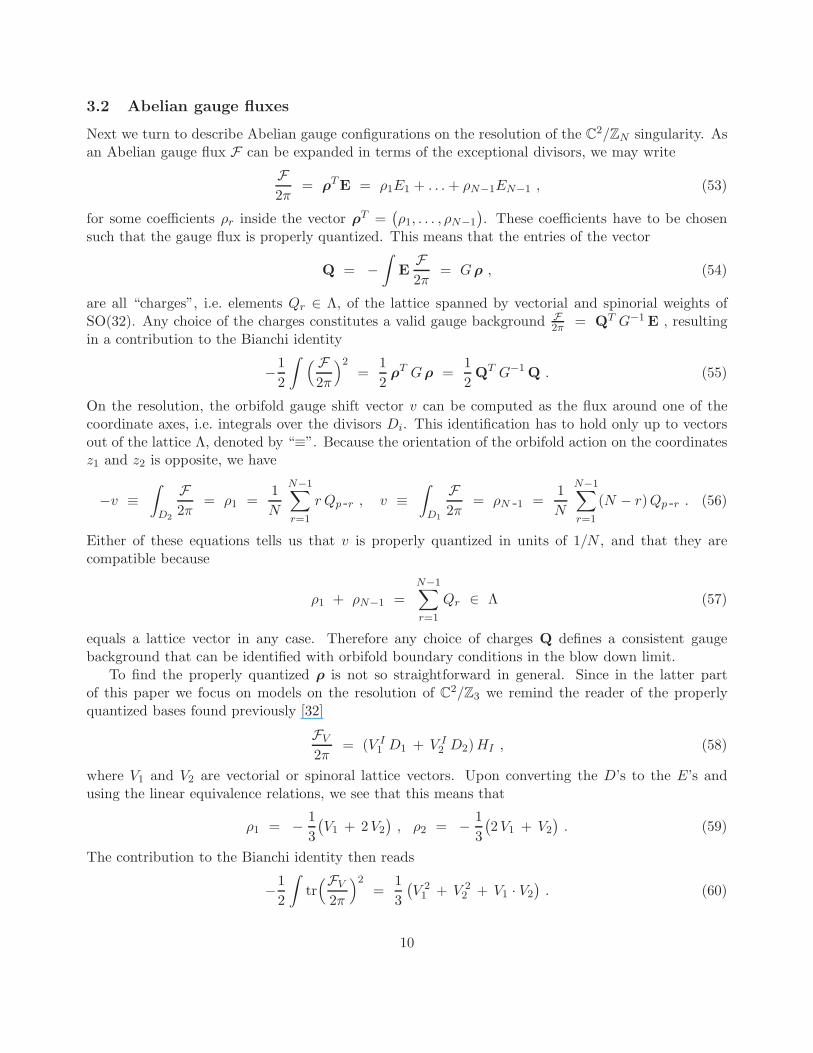
3.2 Abelian gauge fluxes

Next we turn to describe Abelian gauge configurations on the resolution of the C2/ZN singularity. As

an Abelian gauge flux F can be expanded in terms of the exceptional divisors, we may write

F2π

= ρTE = ρ1E1 + . . .+ ρN−1EN−1 , (53)

for some coefficients ρr inside the vector ρT =(ρ1, . . . , ρN−1

). These coefficients have to be chosen

such that the gauge flux is properly quantized. This means that the entries of the vector

Q = −∫

EF2π

= Gρ , (54)

are all “charges”, i.e. elements Qr ∈ Λ, of the lattice spanned by vectorial and spinorial weights ofSO(32). Any choice of the charges constitutes a valid gauge background F

2π = QT G−1 E , resultingin a contribution to the Bianchi identity

−1

2

∫ ( F2π

)2=

1

2ρT Gρ =

1

2QT G−1 Q . (55)

On the resolution, the orbifold gauge shift vector v can be computed as the flux around one of thecoordinate axes, i.e. integrals over the divisors Di. This identification has to hold only up to vectorsout of the lattice Λ, denoted by “≡”. Because the orientation of the orbifold action on the coordinatesz1 and z2 is opposite, we have

−v ≡∫

D2

F2π

= ρ1 =1

N

N−1∑

r=1

r Qp -r , v ≡∫

D1

F2π

= ρN -1 =1

N

N−1∑

r=1

(N − r)Qp -r . (56)

Either of these equations tells us that v is properly quantized in units of 1/N , and that they arecompatible because

ρ1 + ρN−1 =N−1∑

r=1

Qr ∈ Λ (57)

equals a lattice vector in any case. Therefore any choice of charges Q defines a consistent gaugebackground that can be identified with orbifold boundary conditions in the blow down limit.

To find the properly quantized ρ is not so straightforward in general. Since in the latter partof this paper we focus on models on the resolution of C

2/Z3 we remind the reader of the properlyquantized bases found previously [32]

FV2π

= (V I1 D1 + V I

2 D2)HI , (58)

where V1 and V2 are vectorial or spinoral lattice vectors. Upon converting the D’s to the E’s andusing the linear equivalence relations, we see that this means that

ρ1 = − 1

3

(V1 + 2V2

), ρ2 = − 1

3

(2V1 + V2

). (59)

The contribution to the Bianchi identity then reads

−1

2

∫

tr(FV

2π

)2=

1

3

(V 2

1 + V 22 + V1 · V2

). (60)

10

D2D1E2E1

~x2~x1 ~x3

Figure 1: Schematic picture of the compact and non–compact curves within the resolution of C2/Z3

corresponding to the exceptional divisors Er and the ordinary divisors Di, respectively.

3.3 Relation with explicit construction of (non–)Abelian gauge fluxes

In the previous section we have discussed explicit solutions of the non–compact Calabi–Yau conditionand presented explicit constructions of Abelian and non–Abelian gauge backgrounds. Comparing theresults of the Abelian gauge fluxes and the construction of the divisors shows, that we can make iden-tifications between the exceptional and ordinary divisors and the characteristic classes correspondingto the gauge field strength (denoted by [. . .])

2π Er = [Fr] = [Fr − Fr+1] , 2π D1 = [FN ] . 2π D2 = − [F1] . (61)

By the Poincare duality we know that the divisors also have an interpretation as complex curves inthe resolution space. For this we assume that all the centers ~xr, r = 1, . . . N -1, lie ordered on one line.The representation of the exceptional divisors are two–spheres suspended at two adjacent centers [37]

Er =(~x, x4

) ∣∣ x4 ∈ [0, 2πR[ , ~x = ~xr + λ

(~xr+1 − ~xr

), λ ∈ [0, 1]

. (62)

Clearly these surfaces are compact, and only nearest neighbor divisors have non–vanishing intersectionnumber one, as they intersect only at a single point: the center that they both have in common. In asimilar way we can also give a representation of the non–compact ordinary divisors

D1 =(~x, x4

) ∣∣ x4 ∈ [0, 2πR[ , ~x = ~xN + λ~e3 , λ ≥ 0

,

D2 =(~x, x4

) ∣∣ x4 ∈ [0, 2πR[ , ~x = ~x1 − λ~e3 , λ ≥ 0

,(63)

Hence, the intersections D1EN−1 = D2E1 = 1 are consistent with what we found before. The Abeliangauge fluxes are thus associated with the complex curves between two centers of an Eguchi–Hansonspace A schematic picture of these curves and their intersections is sketched in Figure 1.

Non–Abelian bundles on Eguchi–Hanson spaces we can describe by similar pictures. As we haveseen in Subsection 2.3, instantons on Eguchi–Hanson spaces are supported at one or more centersof the Eguchi–Hanson space. In particular, the standard embedding is supported on all centers,and therefore all divisors participate to the total Chern class (52): Precisely because the standardembedding instanton is supported at each of the centers we cannot deform the curves at these points.

Instead, for the instanton I~x2supported only at ~x2, we can merge the curves D2 and E1, because

there is no obstruction created by the instanton. The resulting curve is denoted as D2 +E1. Similarlythe curves D1 and E2 can be merged to form D1 + E2. This process is depicted in Figure 2 forthe C

2/Z3 singularity given in Figure 1. Therefore, as far as the instanton supported only at ~x2 isconcerned, there are only two divisors D2 +E1 and D1 +E2 relevant, and consequently its total Chernclass reads

c(I~x2) = (1 +D2 +E1)(1 +D1 + E2) . (64)

11

D1E2

D1 + E2

E1D2

D2 + E1

~x2

~x2

~x2~x1 ~x3

Figure 2: The two curves D2, E1 and D1, E2 are merged to form the curves D2 + E1 and D1 + E2,respectively.

Because this describes an SU(2) (non–Abelian) flux the first Chern class vanishes identically, as followsdirectly from expanding this to first order and using the linear equivalence relations (50). For thesecond Chern class we find

∫

c2(I~x2) = 1 − 1

N, (65)

using the intersection numbers given above. This is consistent with the result computed in (41) usingthe explicit instanton solution on the Eguchi–Hanson space. One can check that also for instantonssupported at multiple centers this procedure gives the correct value p − 1/N for the second Chernclass, and that this result only depends on the number p of centers present in the instanton, not attheir location.

4 Blowup models on non–compact K3 orbifolds

In the previous two sections we used both explicit constructions and implicit toric geometry methodsto describe the geometry of non–compact resolutions of C

2/ZN orbifolds, and the Abelian and non–Abelian gauge configurations they can support. The purpose of this section is to show that the resultingmodels can be understood as non–compact heterotic orbifold models with certain VEV’s switched on.For concreteness we restrict ourselves to models on the C

2/Z3 orbifold only. The correspondingheterotic orbifold models are listed in Table 1. Below we list the possible smooth models obtainedby combining the Abelian and non–Abelian bundles constructed in the previous sections. Since bydefinition all these configurations are supersymmetric as the gauge backgrounds were required tosatisfy the Hermitian Yang-Mills equations, we restrict ourself to the blow-ups of heterotic C

2/Z3

orbifold models that do not break supersymmetry, thus, we only consider VEV’s along flat directionsof the potential.

We stress the fact that the models we consider are non–compact, but they are built in a waysuch that compact (global) orbifolds can be recovered in the simplest possible way. In particular, we

12

#Gauge group

Shift vector

Untwisted

matter

Twisted

matter

3a SO(28) × SU(2) × U(1) 19 [(28,2)1 + 1(1,1)2 + 2(1,1)0] (28,2)−1/3 + 5(1,1)2/3

13(12, 014) +2(1,1)4/3

3b SO(22) × SU(5) × U(1) 19 [(22,5)1 + (1,10)2 + 2(1,1)0] (22,1)5/3 + (1,10)−4/3

13(14, 2, 011) +2(1,5)−2/3

3c SO(16) × SU(8) × U(1) 19 [(16,8)1 + (1,28)2 + 2(1,1)0] (1,28)−2/3 + 2(1,1)8/3

13(18, 08)

3d SO(10) × SU(11) × U(1) 19 [(10,11)1 + (1,55)2 + 2(1,1)0] (1,11)−8/3 + (16,1)−11/6

13(110, 2, 05)

3e SU(14) × SU(2)2 × U(1) 19 [(14,2,2)1 + (91,1,1)2 + 2(1)0] (1)14/3 + (14,2,1)−4/3

13(114, 02) +2(1,1,2)−7/3

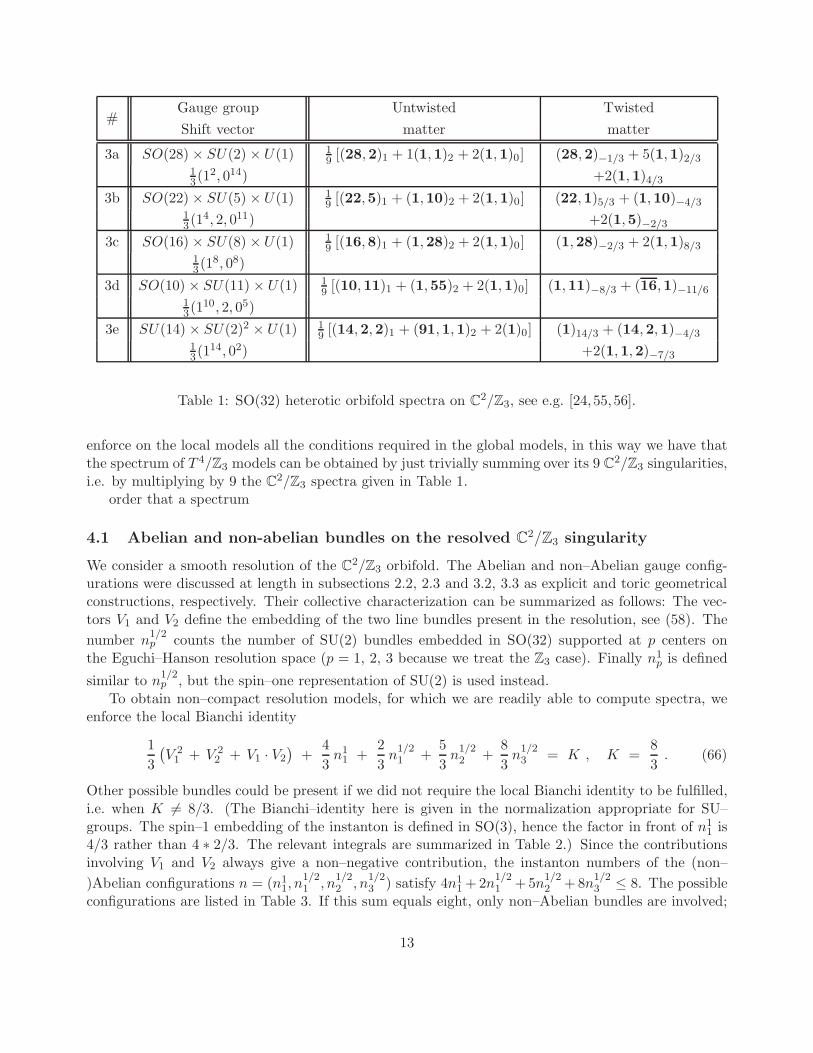
Table 1: SO(32) heterotic orbifold spectra on C2/Z3, see e.g. [24,55,56].

enforce on the local models all the conditions required in the global models, in this way we have thatthe spectrum of T 4/Z3 models can be obtained by just trivially summing over its 9 C

2/Z3 singularities,i.e. by multiplying by 9 the C

2/Z3 spectra given in Table 1.order that a spectrum

4.1 Abelian and non-abelian bundles on the resolved C2/Z3 singularity

We consider a smooth resolution of the C2/Z3 orbifold. The Abelian and non–Abelian gauge config-

urations were discussed at length in subsections 2.2, 2.3 and 3.2, 3.3 as explicit and toric geometricalconstructions, respectively. Their collective characterization can be summarized as follows: The vec-tors V1 and V2 define the embedding of the two line bundles present in the resolution, see (58). The

number n1/2p counts the number of SU(2) bundles embedded in SO(32) supported at p centers on

the Eguchi–Hanson resolution space (p = 1, 2, 3 because we treat the Z3 case). Finally n1p is defined

similar to n1/2p , but the spin–one representation of SU(2) is used instead.

To obtain non–compact resolution models, for which we are readily able to compute spectra, weenforce the local Bianchi identity

1

3

(V 2

1 + V 22 + V1 · V2

)+

4

3n1

1 +2

3n

1/21 +

5

3n

1/22 +

8

3n

1/23 = K , K =

8

3. (66)

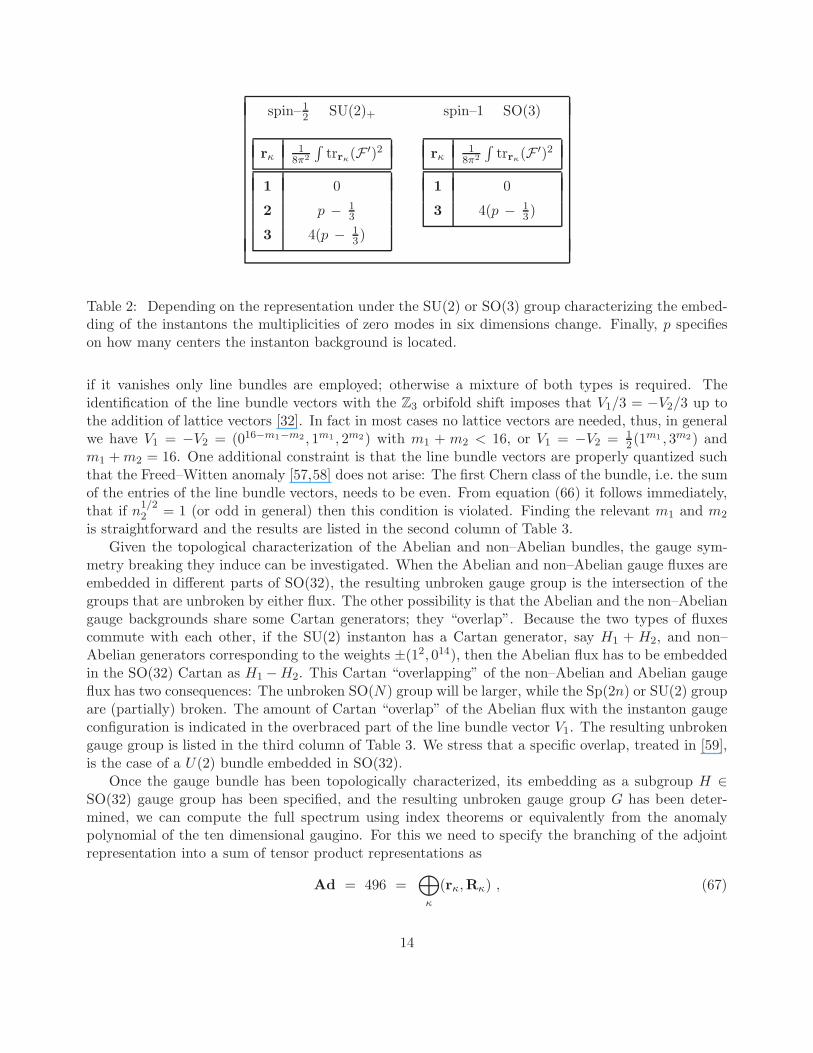
Other possible bundles could be present if we did not require the local Bianchi identity to be fulfilled,i.e. when K 6= 8/3. (The Bianchi–identity here is given in the normalization appropriate for SU–groups. The spin–1 embedding of the instanton is defined in SO(3), hence the factor in front of n1

1 is4/3 rather than 4 ∗ 2/3. The relevant integrals are summarized in Table 2.) Since the contributionsinvolving V1 and V2 always give a non–negative contribution, the instanton numbers of the (non–

)Abelian configurations n = (n11, n

1/21 , n

1/22 , n

1/23 ) satisfy 4n1

1 + 2n1/21 + 5n

1/22 + 8n

1/23 ≤ 8. The possible

configurations are listed in Table 3. If this sum equals eight, only non–Abelian bundles are involved;

13

spin–12 SU(2)+ spin–1 SO(3)

rκ1

8π2

∫trrκ

(F ′)2

1 0

2 p − 13

3 4(p − 13)

rκ1

8π2

∫trrκ

(F ′)2

1 0

3 4(p − 13)

Table 2: Depending on the representation under the SU(2) or SO(3) group characterizing the embed-ding of the instantons the multiplicities of zero modes in six dimensions change. Finally, p specifieson how many centers the instanton background is located.

if it vanishes only line bundles are employed; otherwise a mixture of both types is required. Theidentification of the line bundle vectors with the Z3 orbifold shift imposes that V1/3 = −V2/3 up tothe addition of lattice vectors [32]. In fact in most cases no lattice vectors are needed, thus, in generalwe have V1 = −V2 = (016−m1−m2 , 1m1 , 2m2) with m1 + m2 < 16, or V1 = −V2 = 1

2 (1m1 , 3m2) andm1 +m2 = 16. One additional constraint is that the line bundle vectors are properly quantized suchthat the Freed–Witten anomaly [57,58] does not arise: The first Chern class of the bundle, i.e. the sumof the entries of the line bundle vectors, needs to be even. From equation (66) it follows immediately,that if n

1/22 = 1 (or odd in general) then this condition is violated. Finding the relevant m1 and m2

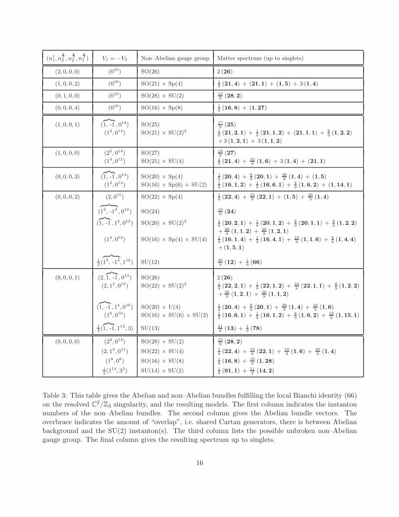
is straightforward and the results are listed in the second column of Table 3.Given the topological characterization of the Abelian and non–Abelian bundles, the gauge sym-

metry breaking they induce can be investigated. When the Abelian and non–Abelian gauge fluxes areembedded in different parts of SO(32), the resulting unbroken gauge group is the intersection of thegroups that are unbroken by either flux. The other possibility is that the Abelian and the non–Abeliangauge backgrounds share some Cartan generators; they “overlap”. Because the two types of fluxescommute with each other, if the SU(2) instanton has a Cartan generator, say H1 + H2, and non–Abelian generators corresponding to the weights ±(12, 014), then the Abelian flux has to be embeddedin the SO(32) Cartan as H1 −H2. This Cartan “overlapping” of the non–Abelian and Abelian gaugeflux has two consequences: The unbroken SO(N) group will be larger, while the Sp(2n) or SU(2) groupare (partially) broken. The amount of Cartan “overlap” of the Abelian flux with the instanton gaugeconfiguration is indicated in the overbraced part of the line bundle vector V1. The resulting unbrokengauge group is listed in the third column of Table 3. We stress that a specific overlap, treated in [59],is the case of a U(2) bundle embedded in SO(32).

Once the gauge bundle has been topologically characterized, its embedding as a subgroup H ∈SO(32) gauge group has been specified, and the resulting unbroken gauge group G has been deter-mined, we can compute the full spectrum using index theorems or equivalently from the anomalypolynomial of the ten dimensional gaugino. For this we need to specify the branching of the adjointrepresentation into a sum of tensor product representations as

Ad = 496 =⊕

κ

(rκ,Rκ) , (67)

14

where rκ and Rκ denote irreducible representations of the non–Abelian part of H and G, respectively.Under the assumption V1 = −V2 = V , we find that the multiplicity Nκ of a state Rκ is determined by

Nκ =1

2

1

(2π)2

∫ 1

2trrκ

(F ′)2 +1

2dim rκ

(

F2V |Rκ

− 1

12trR2

)

, (68)

where F ′ denotes the non–Abelian instanton background, FV the Abelian gauge flux, and R the SU(2)curvature two–form. The integrals over the curvature and the U(1) background follow directly fromthe results of earlier parts of this paper, i.e.

1

8π2

∫

trR2 =8

3,

1

8π2

∫

trF2V =

1

3H2V , (69)

where we denote by HV = VI HI the Cartan generator of the Abelian–bundle. The value of theoperator H2

V has to be evaluated on each of the irreducible representations Rκ as the multiplicitynumber (68) indicates. More care needs to be taken when computing the integral over the non–Abelian instanton background F ′, as it also depends on over which representation rκ the trace istaken. For the spin–1

2 instantons this can be the singlet 1, the fundamental 2, or the adjoint 3,representations of SU(2); for the spin-1 instantons only the singlet or triplet representations of SO(3)are relevant for our purposes. In the cases where there are multiple non–Abelian instantons embedded,also traces over product representations occur. The basic values of the possible instanton numbershave been collected in table 2.

The resulting spectra are given in the last column of Table 3. The computation of these spectrarequires mostly standard group theory, see e.g. [60]. As only the representation theory of the Sp(2n)groups might be less known, we have collected some relevant facts in Appendix A. The spectra for thepure line bundle models agree with those given in Ref. [24]; the other spectra are novel except that ofthe standard embedding.

4.2 Supersymmetric blowups

We study blow-ups of the Z3 heterotic orbifold models, that preserve six dimensional supersymmetryby switching on VEV’s for twisted and possibly also untwisted states, and that can be identified withthe smooth bundle models listed in Table 3. The analysis can be performed entirely at the classicallevel, because in six dimensional super–Yang–Mills theory dangerous loop corrections to the potentialare absent. (This is of course unlike the four dimensional case, where one-loop Fayet–Iliopouloscorrections may arise.)

The study of flat directions of the potential V involves the three real auxiliary fields, Dia with

i = 1, 2, 3, of six dimensional super Yang–Mills theory

V =1

2

∑

i,a

(Dia)

2 , Dia = σiαβ φ

†α Taφβ , (70)

where the representation indices on the complex scalar components φ1, φ2 of a hypermultiplet andgauge generator Ta have been suppressed. It turns out convenient to use four dimensional N = 1notation of a real D–term Da = D3

a and a complex F–term Fa = (D1a + iD2

a)/√

2. Since the complexscalar φ1 and φ2 components of hypermultiplets are in complex conjugate representations, we have

V =1

2

∑

a

D2a +

∑

a

FaFa , Da = φ1Taφ1 − φ2Taφ2 , Fa = φ2Taφ1 . (71)

15

(n1

1, n1

2

3, n

1

2

2, n

1

2

1) V1 = −V2 Non–Abelian gauge group Matter spectrum (up to singlets)

(2, 0, 0, 0) (016) SO(26) 2 (26)

(1, 0, 0, 2) (016) SO(21) × Sp(4) 1

9(21, 4) + (21, 1) + (1,5) + 3 (1,4)

(0, 1, 0, 0) (016) SO(28) × SU(2) 10

9(28,2)

(0, 0, 0, 4) (016) SO(16) × Sp(8) 1

9(16, 8) + (1,27)

(1, 0, 0, 1) (z|

1, -1 , 014) SO(25) 17

9(25)

(12, 014) SO(21) × SU(2)2 1

9(21, 2,1) + 1

9(21,1,2) + (21,1, 1) + 8

9(1, 2,2)

+3 (1,2,1) + 3 (1,1,2)

(1, 0, 0, 0) (22, 014) SO(27) 19

9(27)

(14, 012) SO(21) × SU(4) 1

9(21, 4) + 10

9(1,6) + 3 (1,4) + (21,1)

(0, 0, 0, 3) (z|

1, -1 , 014) SO(20) × Sp(4) 1

9(20, 4) + 8

9(20,1) + 28

9(1,4) + (1,5)

(12, 014) SO(16) × Sp(6) × SU(2) 1

9(16, 1,2) + 1

9(16,6,1) + 8

9(1,6, 2) + (1,14,1)

(0, 0, 0, 2) (2, 015) SO(22) × Sp(4) 1

9(22, 4) + 10

9(22,1) + (1,5) + 26

9(1,4)

(z |

12, -12

, 012) SO(24) 16

9(24)

(z|

1, -1 , 12, 012) SO(20) × SU(2)2 1

9(20, 2,1) + 1

9(20,1,2) + 8

9(20,1, 1) + 8

9(1,2,2)

+ 28

9(1,1,2) + 28

9(1,2,1)

(14, 012) SO(16) × Sp(4) × SU(4) 1

9(16, 1,4) + 1

9(16,4,1) + 10

9(1,1,6) + 8

9(1,4,4)

+ (1, 5,1)

1

2(z |

12, -12

, 112) SU(12) 20

9(12) + 1

9(66)

(0, 0, 0, 1) (2,z|

1, -1 , 013) SO(26) 2 (26)

(2, 12, 013) SO(22) × SU(2)2 1

9(22, 2,1) + 1

9(22,1,2) + 10

9(22,1,1) + 8

9(1,2, 2)

+ 26

9(1,2,1) + 26

9(1,1,2)

(z|

1, -1 , 14, 010) SO(20) × U(4) 1

9(20, 4) + 8

9(20,1) + 28

9(1,4) + 10

9(1,6)

(16, 010) SO(16) × SU(6) × SU(2) 1

9(16, 6,1) + 1

9(16,1,2) + 8

9(1,6, 2) + 10

9(1,15, 1)

1

2(z|

1, -1, 113, 3) SU(13) 21

9(13) + 1

9(78)

(0, 0, 0, 0) (22, 014) SO(28) × SU(2) 10

9(28,2)

(2, 14, 011) SO(22) × SU(4) 1

9(22, 4) + 10

9(22,1) + 10

9(1,6) + 26

9(1,4)

(18, 08) SO(16) × SU(8) 1

9(16, 8) + 10

9(1,28)

1

2(114, 32) SU(14) × SU(2) 1

9(91, 1) + 11

9(14,2)

Table 3: This table gives the Abelian and non–Abelian bundles fulfilling the local Bianchi identity (66)on the resolved C

2/Z3 singularity, and the resulting models. The first column indicates the instantonnumbers of the non–Abelian bundles. The second column gives the Abelian bundle vectors. Theoverbrace indicates the amount of “overlap”, i.e. shared Cartan generators, there is between Abelianbackground and the SU(2) instanton(s). The third column lists the possible unbroken non–Abeliangauge group. The final column gives the resulting spectrum up to singlets.

16

(n1

1, n1

2

3, n

1

2

2, n

1

2

1) V1 = −V2 Unbroken gauge group # Twisted Untwisted

(2, 0, 0, 0) (016) SO(26) 3a (28,2), (1)

(1, 0, 0, 2) (016) SO(21) × Sp(4) 3b (22,1), (1,10) (22,5)

(0, 1, 0, 0) (016) SO(28) × SU(2) 3a 2 × (1)

(0, 0, 0, 4) (016) SO(16) × Sp(8) 3c (1,28), (1)

(1,28), (1) (1,28)

(1, 0, 0, 1) (z|

1, -1 , 014) SO(25) 3a (28,2), (1) (28,2)

(12, 014) SO(21) × SU(2) × SU(2) 3b (22,1), (1,10), (1,5) (1,10)

(1, 0, 0, 0) (2, 015) SO(27) 3a (28,2), (1) (28,2)

(14, 012) SO(21) × SU(4) 3b (22,1), (1,5) (22,5)

(0, 0, 0, 3) (z|

1, -1 , 014) SO(20) × Sp(4) 3b (22,1), (1,10) (22,5)

(12, 014) SO(16) × Sp(6) × SU(2) 3c (1,28), (1) (1,28)

(0, 0, 0, 2) (2, 015) SO(22) × Sp(4) 3b (1,10), (1,5)

(1,10), (1,5) (1,10)

(z |

12, -12

, 012) SO(24) 3a (28,2), (1) (28,2)

(z|

1, -1 , 12, 012) SO(20) × SU(2)2 3b (22,1), (1,10) (22,5), (1, 10)

(14, 012) SO(16) × Sp(4) × SU(4) 3c (1,28), (1) (1,28)

1

2(z |

12, -12

, 112) SU(12) 3e (14,2,1), (2,1,1), (1) (14,2, 2)

(0, 0, 0, 1) (2,z|

1, -1 , 013) SO(26) 3a (28,2), (1)

(2, 12, 013) SO(22) × SU(2)2 3b (1,10), (1,5) (1,10)

(z|

1, -1 , 14, 010) SO(20) × U(4) 3b (22,1), (1,5) (22,5)

(16, 010) SO(16) × SU(2) × SU(6) 3c (1,28), (1) (1,28)

1

2(z|

1, -1, 113, 3) SU(13) 3e (14,2,1), (2,1,1), (1) (14,2, 2)

(0, 0, 0, 0) (22, 014) SO(28) × SU(2) 3a 2 × (1)

(2, 14, 011) SO(22) × SU(4) 3b 2 × (1,5)

(18, 08) SO(16) × SU(8) 3c 2 × (1)1

2(114, 32) SU(14) × SU(2) 3e 2 × (1,1,2)

Table 4: The first three columns contain the same information as Table 3. The final columns indicatefrom which of five heterotic Z3 models, listed in Table 1, these bundle models can be obtained byswitching on VEV’s for the indicated twisted and untwisted states.

17

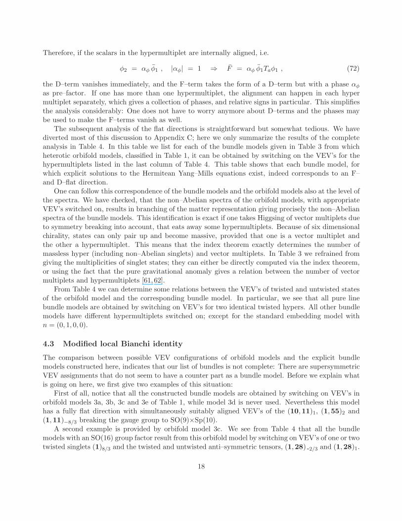
Therefore, if the scalars in the hypermultiplet are internally aligned, i.e.

φ2 = αφ φ1 , |αφ| = 1 ⇒ F = αφ φ1Taφ1 , (72)

the D–term vanishes immediately, and the F–term takes the form of a D–term but with a phase αφas pre–factor. If one has more than one hypermultiplet, the alignment can happen in each hypermultiplet separately, which gives a collection of phases, and relative signs in particular. This simplifiesthe analysis considerably: One does not have to worry anymore about D–terms and the phases maybe used to make the F–terms vanish as well.

The subsequent analysis of the flat directions is straightforward but somewhat tedious. We havediverted most of this discussion to Appendix C; here we only summarize the results of the completeanalysis in Table 4. In this table we list for each of the bundle models given in Table 3 from whichheterotic orbifold models, classified in Table 1, it can be obtained by switching on the VEV’s for thehypermultiplets listed in the last column of Table 4. This table shows that each bundle model, forwhich explicit solutions to the Hermitean Yang–Mills equations exist, indeed corresponds to an F–and D–flat direction.

One can follow this correspondence of the bundle models and the orbifold models also at the level ofthe spectra. We have checked, that the non–Abelian spectra of the orbifold models, with appropriateVEV’s switched on, results in branching of the matter representation giving precisely the non–Abelianspectra of the bundle models. This identification is exact if one takes Higgsing of vector multiplets dueto symmetry breaking into account, that eats away some hypermultiplets. Because of six dimensionalchirality, states can only pair up and become massive, provided that one is a vector multiplet andthe other a hypermultiplet. This means that the index theorem exactly determines the number ofmassless hyper (including non–Abelian singlets) and vector multiplets. In Table 3 we refrained fromgiving the multiplicities of singlet states; they can either be directly computed via the index theorem,or using the fact that the pure gravitational anomaly gives a relation between the number of vectormultiplets and hypermultiplets [61,62].

From Table 4 we can determine some relations between the VEV’s of twisted and untwisted statesof the orbifold model and the corresponding bundle model. In particular, we see that all pure linebundle models are obtained by switching on VEV’s for two identical twisted hypers. All other bundlemodels have different hypermultiplets switched on; except for the standard embedding model withn = (0, 1, 0, 0).

4.3 Modified local Bianchi identity

The comparison between possible VEV configurations of orbifold models and the explicit bundlemodels constructed here, indicates that our list of bundles is not complete: There are supersymmetricVEV assignments that do not seem to have a counter part as a bundle model. Before we explain whatis going on here, we first give two examples of this situation:

First of all, notice that all the constructed bundle models are obtained by switching on VEV’s inorbifold models 3a, 3b, 3c and 3e of Table 1, while model 3d is never used. Nevertheless this modelhas a fully flat direction with simultaneously suitably aligned VEV’s of the (10,11)1, (1,55)2 and(1,11)−8/3 breaking the gauge group to SO(9)×Sp(10).

A second example is provided by orbifold model 3c. We see from Table 4 that all the bundlemodels with an SO(16) group factor result from this orbifold model by switching on VEV’s of one or twotwisted singlets (1)8/3 and the twisted and untwisted anti–symmetric tensors, (1,28) -2/3 and (1,28)1.

18

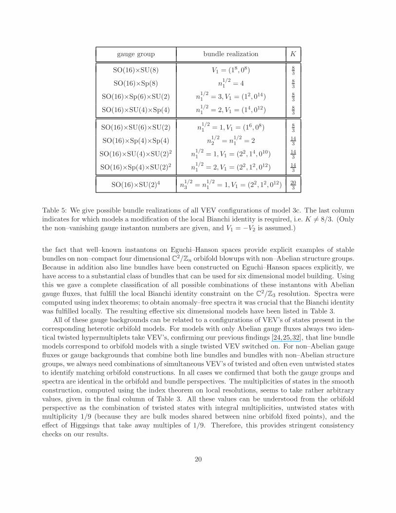
Following the analysis of Appendix C one concludes that with these multiplets taking VEV’s thepossible unbroken gauge group could be any of the ones listed in Table 5. These different possibilitiesarise because of the VEV’s for the anti–symmetric tensors: They can be skew–diagonalized. Thendepending on whether some or all of its diagonal entries are equal and / or zero, one of the abovementioned gauge groups is realized. (For example: All entries zero gives SU(8), all entries equal butnon–zero gives Sp(8), and finally all entries different gives SU(2)4.) Table 3 does not contain the gaugegroup factors Sp(4)×Sp(4), SU(4)×SU(2)2, Sp(4)×SU(2)2 and SU(2)4, hence there are bundle modelsmissing.

As a side remark we note, that this example also shows that many different bundle models, char-acterized by different topological parameters are actually related to each other by continuous de-formations of the VEV’s of twisted and untwisted states of the corresponding orbifold model. Theprecise relation between the moduli space of VEV configurations and bundle models is beyond thescope of this paper. Presumably this requires to analyze the full gauge bundle moduli space using theADHM [44,45] and Kronheimer–Nakajima [46–48] constructions, see e.g. [36,37,49,63].

Bundle realizations of these and other VEV configurations of orbifold models can be obtainedrealizing that the local Bianchi identity (66) is a sufficient condition to uncover consistent models butcertainly not a necessary condition. Indeed, only on a compact K3 the integrated Bianchi identityneeds to vanish. This means that if one has a compact orbifold, say like T 4/Z3, the sum of theinstanton numbers from all fixed points needs to equal 24. The local Bianchi identity (66) is obtainedby splitting up the total instanton number of K3 equally over all 9 fixed points of T 4/Z3. The totalinstanton number 24 cannot be completely arbitrarily distributed over the various fixed points, sincethe instanton number is quantized itself [55, 64, 65]: The basic unit of instanton number that can bemoved around equals 1. This means that the local Bianchi identity (66) equals K = 8/3 mod 1. Theadditional constraint, that the first Chern class of the bundle is even, implies that K = 8/3 mod 2,

unless n1/22 is odd. This coincides precisely with the (weak) modular invariance condition for a local

orbifold shift vector.The smallest local Bianchi identity has K = 2/3 in (66). There are two solutions to this equation:

i) n1/21 = 1, V1 = V2 = 0, which results in the unbroken gauge group SO(28)×SU(2), and ii) n

1/21 = 0,

V1 = −V2 = (12, 014), with unbroken gauge group SO(28)×SU(2). Thus both are VEV configurationsof orbifold model 3a, which we had already found.

Using the modified Bianchi identity, eq. (66) for an instanton numberK = 14/3 a bundle realization

of the VEV configuration of model 3d can be found: The bundle is characterized by n11 = 1 and n

1/21 =

5. Also the VEV configurations of 3c with gauge groups Sp(4)×Sp(4), SU(4)×SU(2)2, Sp(4)×SU(2)2

and SU(2)4, discussed above, can be identified. For each of these models we give a bundle candidatein Table 5. To compute the spectra of these models is challenging because for that we need a modifiedindex theorem that takes the non–vanishing three–form flux H3 into account. Indeed, using thestandard index theorem ensures an anomaly–free spectrum only in case the Bianchi identity is fulfilled[61,66].

5 Conclusions and outlook

The construction of stable non–Abelian bundles on Calabi–Yau manifolds is one of the outstandingproblems in both mathematics and theoretical physics. Yet to determine the full phenomenologicalpotential of heterotic string constructions this is of fundamental importance. In this paper we exploited

19

gauge group bundle realization K

SO(16)×SU(8) V1 = (18, 08) 83

SO(16)×Sp(8) n1/21 = 4 8

3

SO(16)×Sp(6)×SU(2) n1/21 = 3, V1 = (12, 014) 8

3

SO(16)×SU(4)×Sp(4) n1/21 = 2, V1 = (14, 012) 8

3

SO(16)×SU(6)×SU(2) n1/21 = 1, V1 = (16, 08) 8

3

SO(16)×Sp(4)×Sp(4) n1/22 = n

1/21 = 2 14

3

SO(16)×SU(4)×SU(2)2 n1/21 = 1, V1 = (22, 14, 010) 14

3

SO(16)×Sp(4)×SU(2)2 n1/21 = 2, V1 = (22, 12, 012) 14

3

SO(16)×SU(2)4 n1/23 = n

1/21 = 1, V1 = (22, 12, 012) 20

3

Table 5: We give possible bundle realizations of all VEV configurations of model 3c. The last columnindicates for which models a modification of the local Bianchi identity is required, i.e. K 6= 8/3. (Onlythe non–vanishing gauge instanton numbers are given, and V1 = −V2 is assumed.)

the fact that well–known instantons on Eguchi–Hanson spaces provide explicit examples of stablebundles on non–compact four dimensional C

2/Zn orbifold blowups with non–Abelian structure groups.Because in addition also line bundles have been constructed on Eguchi–Hanson spaces explicitly, wehave access to a substantial class of bundles that can be used for six dimensional model building. Usingthis we gave a complete classification of all possible combinations of these instantons with Abeliangauge fluxes, that fulfill the local Bianchi identity constraint on the C

2/Z3 resolution. Spectra werecomputed using index theorems; to obtain anomaly–free spectra it was crucial that the Bianchi identitywas fulfilled locally. The resulting effective six dimensional models have been listed in Table 3.

All of these gauge backgrounds can be related to a configurations of VEV’s of states present in thecorresponding heterotic orbifold models. For models with only Abelian gauge fluxes always two iden-tical twisted hypermultiplets take VEV’s, confirming our previous findings [24,25,32], that line bundlemodels correspond to orbifold models with a single twisted VEV switched on. For non–Abelian gaugefluxes or gauge backgrounds that combine both line bundles and bundles with non–Abelian structuregroups, we always need combinations of simultaneous VEV’s of twisted and often even untwisted statesto identify matching orbifold constructions. In all cases we confirmed that both the gauge groups andspectra are identical in the orbifold and bundle perspectives. The multiplicities of states in the smoothconstruction, computed using the index theorem on local resolutions, seems to take rather arbitraryvalues, given in the final column of Table 3. All these values can be understood from the orbifoldperspective as the combination of twisted states with integral multiplicities, untwisted states withmultiplicity 1/9 (because they are bulk modes shared between nine orbifold fixed points), and theeffect of Higgsings that take away multiples of 1/9. Therefore, this provides stringent consistencychecks on our results.

20

We have shown that each combination of instantons and Abelian gauge fluxes that fulfill thelocal Bianchi identity corresponds to a VEV configuration of a certain heterotic orbifold. One maywonder whether one can reverse the statement: Each supersymmetric system of VEV’s correspondto a configuration of instantons and gauge fluxes. Presumably this statement is true, but certainlynot all these configurations satisfy the local Bianchi identities. Indeed, we observed that model 3d ofTable 1 is not used at all as an orbifold realization of a bundle model that satisfies this condition, seeTable 4, even though it definitely possesses flat directions. If we give up the local Bianchi identity andallow that it differs by some instanton units, a configuration can be identified that leads to the samegauge group as one obtains from the VEV configuration. To confirm the matching on the level ofthe spectra is hampered by the fact, that index theorems on non–compact spaces cannot be employedwhen the local Bianchi is not satisfied. A generalization of the index theorem in the presence of thecorresponding three form H–flux is needed.

The situation is similar for the possible VEV configurations of the other orbifold models. Forconcreteness we focused on model 3c: Only some of its VEV configurations are realized as bundlemodels satisfying the local Bianchi identity. Other VEV assignments can only be realized, when it isonly fulfilled up to a number of instanton units. The resulting Bianchi identity is then very similar tothe modular invariance condition of heterotic orbifolds. All these different bundle models correspondto VEV configurations which are all continuously connected to each other. Different bundle modelsoften only correspond to very similar VEV configurations, except that in one case the VEVs are equal,in the other they are different. One does not need to take large numbers of VEVs to zero to interpolatebetween such configurations, therefore these transitions are deformations of the bundle rather thanflops. In light of this one may wonder what the topological classification of the bundles exactly means.The description of bundles on Eguchi–Hanson spaces employed by us is not the most general: TheKronheimer–Nakajima construction [47] describes the full moduli space on such ALE gravitationalinstantons, and might therefore be a more appropriate setting for this comparison.

Most of the findings reported in this work relied on the crucial fact that on Eguchi–Hanson spaces,Abelian gauge backgrounds and non–Abelian instanton configurations are known. Explicit resolutionsof C

3/Zn for n > 3 orbifolds are not known, hence to have access to bundles with non–Abelian structuregroups on C

3/Zn resolutions is much more challenging. (Of course one always has the standardembedding, but precisely since it immediately fulfills the local Bianchi identity, it only correspondsto one configuration.) Yet this is of great importance because there are certain six dimensionalorbifolds, like the T 6/Z6–II for which a large pool of MSSM–like models have been constructed recently.Resolutions of generic C

3/Zn orbifolds and their line bundles are only known in toric geometry. In thehope to find a framework that allows us to describe stable bundles with non–Abelian structure groupson toric resolutions of such orbifold singularities, we reformulated the description of the Eguchi–Hansoninstantons in terms of a toric geometry–like language.

Acknowledgments

We would like to thank Massimo Bianchi, Kang–Sin Choi, Tae-Won Ha, Arthur Hebecker, MaximilianKreuzer, Michael Ratz, Emanuel Scheidegger, Stefan Vandoren and Jenny Wagner for stimulatingdiscussions and correspondence. F.P.C. is grateful to the Institut fur Theoretische Physik, Heidelberg,Germany, for support and hospitality during visits in the early stage of this work. The work of F.P.Cis supported by FCT through the grant SFRH/BPD/20667/2004. The work of MT is supported bythe European Community through the contract N 041273 (Marie Curie Intra-European Fellowships).

21

He is also partially supported by the ANR grant ANR-05-BLAN-0079-02, the RTN contracts MRTN-CT-2004-005104 and MRTN-CT-2004-503369, the CNRS PICS # 2530, 3059 and 3747, and by theEuropean Union Excellence Grant MEXT-CT-2003-509661.

A Some Sp(2n) representation theory

This Appendix is devoted to some elementary properties of representation of Sp(2n) groups and howthey arise in branching from SO(4n) groups. Sp(2n) groups are less common in physics, for that reasonwe review the properties that we need here. (See for a more extensive discussion Ref. [67].) The groupSp(2n) is defined as the group of real matrices that leave a symplectic form (anti–symmetric 2n× 2nmatrix) Ω invariant

ST ΩS = Ω , Ω = 11n ⊗ ǫ =

(0 11n

−11n 0

)

. (A.1)

The form of the symplectic matrix Ω given here can be obtained by a suitable basis choice. Alterna-tively one can define this group as the set of unitary matrices U ∈ SU(2n) that leave this symplecticform invariant U †ΩU = Ω. This group is then also often referred to as USp(2n), both definitions infact define the same abstract group.

We list the basic representations of Sp(2n). Since Sp(2n) is defined as a matrix group, its fun-damental representation is the 2n component vector representation 2n on which these matrices actnaturally. The adjoint representation is defined as the algebra of the group. Writing an algebraelement A as a block matrix, we find that its matrix blocks satisfy

A =

(α βγ δ

)

, βT = β , γT = γ , δ = − αT . (A.2)

Therefore the adjoint consists of n(2n + 1) components in total. This corresponds to symmetricHermitian 2n×2n matrices, that are the generators of Sp(2n) as a subgroup of the unitary group. Wecan also consider the anti–symmetric Hermitian matrices. This does not give directly an irreduciblerepresentation because the symplectic form Ω itself is anti–symmetric. Using it we can define thetraceless anti–symmetric representation [2n]2 with n(2n− 1) − 1 components. These representationsfor Sp(2n) groups up to n = 5 are collected in Table 6.

To compute the spectra of models when Sp–groups appear in the main part of the text the branch-ing of SO(4n) and SU(2n) to Sp(2n) are crucial. The relevant branching rules read

SO(4n) → Sp(2n) × SU(2) ,

4n → (2n,2) ,

2n(4n − 1) → (n(2n + 1),1) + (1,3) + (n(2n -1) -1,3) ,

(A.3)

and

SU(2n) → Sp(2n) ,

2n → 2n ,

n(2n -1) → (n(2n -1) -1) + (1) ,

4n2 -1 → (n(2n + 1)) + (n(2n -1) -1) .

(A.4)

22

n 1 2 3 4 5

Sp(2n) Sp(2) Sp(4) Sp(6) Sp(8) Sp(10)

Fund = 2n 2 4 6 8 10

Ad = n(2n + 1) 3 10 21 36 55

[2n]2 = n(2n -1) -1 - 5 14 27 48

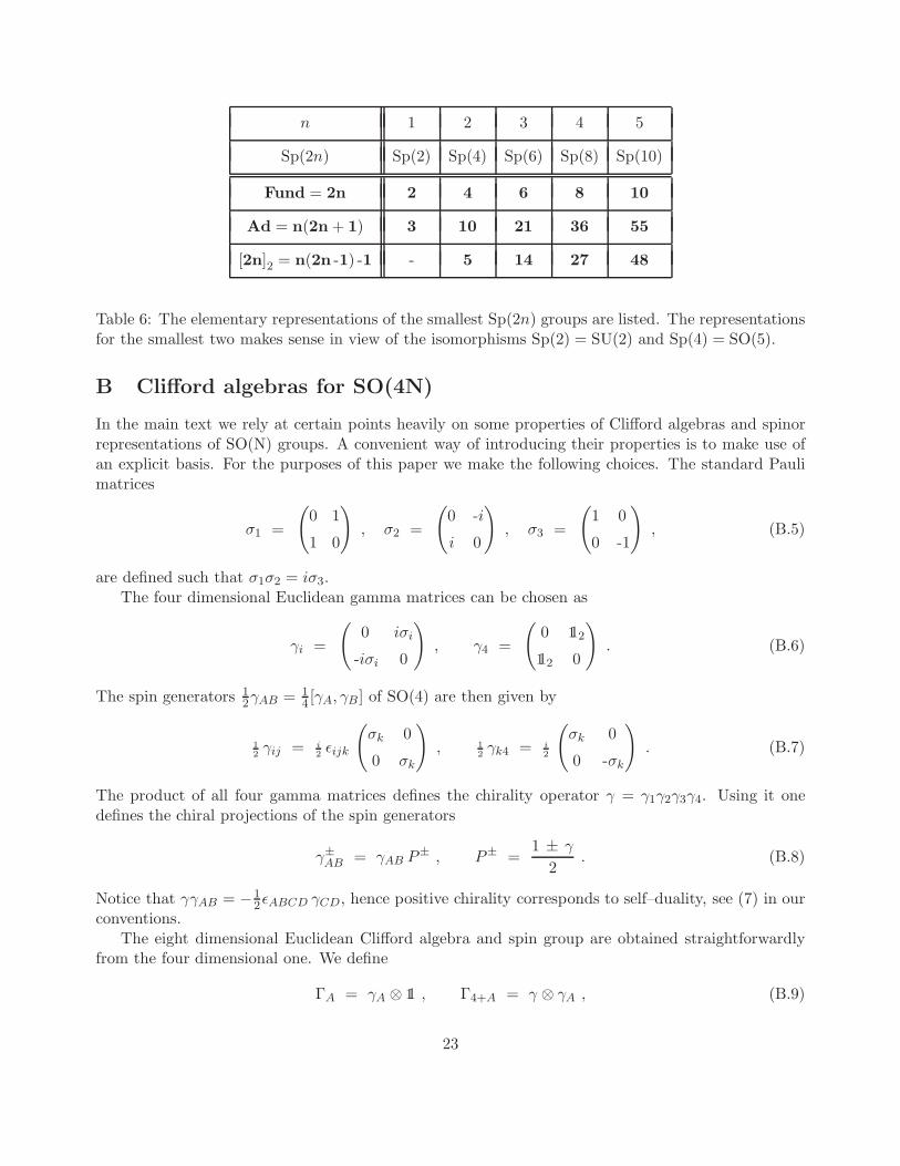
Table 6: The elementary representations of the smallest Sp(2n) groups are listed. The representationsfor the smallest two makes sense in view of the isomorphisms Sp(2) = SU(2) and Sp(4) = SO(5).

B Clifford algebras for SO(4N)

In the main text we rely at certain points heavily on some properties of Clifford algebras and spinorrepresentations of SO(N) groups. A convenient way of introducing their properties is to make use ofan explicit basis. For the purposes of this paper we make the following choices. The standard Paulimatrices

σ1 =

(

0 1

1 0

)

, σ2 =

(

0 -i

i 0

)

, σ3 =

(

1 0

0 -1

)

, (B.5)

are defined such that σ1σ2 = iσ3.The four dimensional Euclidean gamma matrices can be chosen as

γi =

(

0 iσi

-iσi 0

)

, γ4 =

(

0 112

112 0

)

. (B.6)

The spin generators 12γAB = 1

4 [γA, γB ] of SO(4) are then given by

1

2γij = i

2ǫijk

(

σk 0

0 σk

)

, 1

2γk4 = i

2

(

σk 0

0 -σk

)

. (B.7)

The product of all four gamma matrices defines the chirality operator γ = γ1γ2γ3γ4. Using it onedefines the chiral projections of the spin generators

γ±AB = γAB P± , P± =

1 ± γ

2. (B.8)

Notice that γγAB = −12ǫABCD γCD, hence positive chirality corresponds to self–duality, see (7) in our

conventions.The eight dimensional Euclidean Clifford algebra and spin group are obtained straightforwardly

from the four dimensional one. We define

ΓA = γA ⊗ 11 , Γ4+A = γ ⊗ γA , (B.9)

23

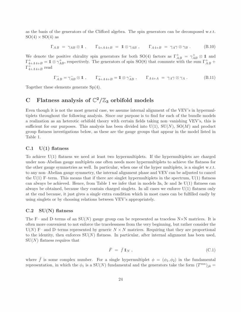
as the basis of the generators of the Clifford algebra. The spin generators can be decomposed w.r.t.SO(4) × SO(4) as

ΓAB = γAB ⊗ 11 , Γ4+A 4+B = 11 ⊗ γAB , ΓA 4+B = γAγ ⊗ γB . (B.10)

We denote the positive chirality spin generators for both SO(4) factors as Γ+AB = γ+

AB ⊗ 11 andΓ+

4+A 4+B = 11 ⊗ γ+AB , respectively. The generators of spin SO(8) that commute with the sum Γ+

AB +

Γ+4+A 4+B read

Γ−AB = γ−AB ⊗ 11 , Γ−

4+A 4+B = 11 ⊗ γ−AB , ΓA 4+A = γAγ ⊗ γA . (B.11)

Together these elements generate Sp(4).

C Flatness analysis of C2/Z3 orbifold models

Even though it is not the most general case, we assume internal alignment of the VEV’s in hypermul-tiplets throughout the following analysis. Since our purpose is to find for each of the bundle modelsa realization as an heterotic orbifold theory with certain fields taking non–vanishing VEV’s, this issufficient for our purposes. This analysis has been divided into U(1), SU(N), SO(M) and productgroup flatness investigations below, as these are the gauge groups that appear in the model listed inTable 1.

C.1 U(1) flatness

To achieve U(1) flatness we need at least two hypermultiplets. If the hypermultiplets are chargedunder non–Abelian gauge multiplets one often needs more hypermultiplets to achieve the flatness forthe other gauge symmetries as well. In particular, when one of the hyper multiplets, is a singlet w.r.t.to any non–Abelian gauge symmetry, the internal alignment phase and VEV can be adjusted to cancelthe U(1) F–term. This means that if there are singlet hypermultiplets in the spectrum, U(1) flatnesscan always be achieved. Hence, from Table 1 we infer that in models 3a, 3c and 3e U(1) flatness canalways be obtained, because they contain charged singlets. In all cases we enforce U(1) flatness onlyat the end because, it just gives a single extra condition which in most cases can be fulfilled easily byusing singlets or by choosing relations between VEV’s appropriately.

C.2 SU(N) flatness

The F– and D–terms of an SU(N) gauge group can be represented as traceless N×N matrices. It isoften more convenient to not enforce the tracelessness from the very beginning, but rather consider theU(N) F– and D–terms represented by generic N ×N matrices. Requiring that they are proportionalto the identity, then enforces SU(N) flatness. In particular, after internal alignment has been used,SU(N) flatness requires that

F = f 11N , (C.1)

where f is some complex number. For a single hypermultiplet φ = (φ1, φ2) in the fundamentalrepresentation, in which the φ1 is a SU(N) fundamental and the generators take the form (Tmn)jk =

24

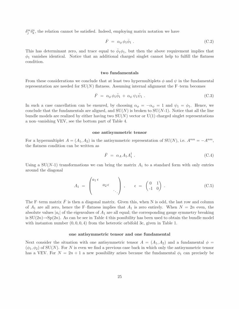
δmj δnk , the relation cannot be satisfied. Indeed, employing matrix notation we have

F = αφ φ1φ1 . (C.2)

This has determinant zero, and trace equal to φ1φ1, but then the above requirement implies thatφ1 vanishes identical. Notice that an additional charged singlet cannot help to fulfill the flatnesscondition.

two fundamentals

From these considerations we conclude that at least two hypermultiplets φ and ψ in the fundamentalrepresentation are needed for SU(N) flatness. Assuming internal alignment the F–term becomes

F = αφ φ1φ1 + αψ ψ1ψ1 . (C.3)

In such a case cancellation can be ensured, by choosing αφ = −αψ = 1 and ψ1 = φ1. Hence, weconclude that the fundamentals are aligned, and SU(N) is broken to SU(N -1). Notice that all the linebundle models are realized by either having two SU(N) vector or U(1) charged singlet representationsa non–vanishing VEV, see the bottom part of Table 4.

one antisymmetric tensor

For a hypermultiplet A = (A1, A2) in the antisymmetric representation of SU(N), i.e. Amn = −Anm,the flatness condition can be written as

F = αAA1A†1 . (C.4)

Using a SU(N -1) transformations we can bring the matrix A1 to a standard form with only entriesaround the diagonal

A1 =

a1 ǫa2 ǫ

. . .

, ǫ =

(0 1-1 0

)

. (C.5)

The F–term matrix F is then a diagonal matrix. Given this, when N is odd, the last row and columnof A1 are all zero, hence the F–flatness implies that A1 is zero entirely. When N = 2n even, theabsolute values |ai| of the eigenvalues of A1 are all equal; the corresponding gauge symmetry breakingis SU(2n)→Sp(2n). As can be see in Table 4 this possibility has been used to obtain the bundle modelwith instanton number (0, 0, 0, 4) from the heterotic orbifold 3c, given in Table 1.

one antisymmetric tensor and one fundamental

Next consider the situation with one antisymmetric tensor A = (A1, A2) and a fundamental φ =(φ1, φ2) of SU(N). For N is even we find a previous case back in which only the antisymmetric tensorhas a VEV. For N = 2n + 1 a new possibility arises because the fundamental φ1 can precisely be

25

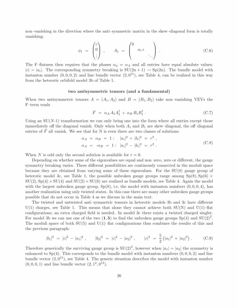
non–vanishing in the direction where the anti–symmetric matrix in the skew–diagonal form is totallyvanishing:

φ1 =

c0...

, A1 =

0a1 ǫ

. . .

. (C.6)

The F–flatness then requires that the phases αφ = αA and all entries have equal absolute values:|c| = |ai|. The corresponding symmetry breaking is SU(2n + 1) → Sp(2n). The bundle model withinstanton number (0, 0, 0, 2) and line bundle vector (2, 015), see Table 4, can be realized in this wayfrom the heterotic orbifold model 3b of Table 1.

two antisymmetric tensors (and a fundamental)

When two antisymmetric tensors A = (A1, A2) and B = (B1, B2) take non–vanishing VEVs theF–term reads

F = αAA1A†1 + αB B1B

†1 . (C.7)

Using an SU(N -1) transformation we can only bring one into the form where all entries except thoseimmediately off the diagonal vanish. Only when both A1 and B1 are skew–diagonal, the off–diagonalentries of F all vanish. We see that for N is even there are two classes of solutions:

αA = αB = 1 : |ai|2 + |bi|2 = r2 ,

αA = -αB = 1 : |ai|2 − |bi|2 = r2 .(C.8)

When N is odd only the second solution is available for r = 0.Depending on whether some of the eigenvalues are equal and non–zero, zero or different, the gauge

symmetry breaking varies. These different possibilities are continously connected in the moduli spacebecause they are obtained from varying some of these eigenvalues. For the SU(8) gauge group ofheterotic model 3c, see Table 1, the possible unbroken gauge groups range among Sp(8),Sp(6) ×SU(2),Sp(4)× SU(4) and SU(2)× SU(6) are realized as bundle models, see Table 4. Again the modelwith the largest unbroken gauge group, Sp(8), i.e. the model with instanton numbers (0, 0, 0, 4), hasanother realization using only twisted states. In this case there are many other unbroken gauge groupspossible that do not occur in Table 4 as we discuss in the main text.

The twisted and untwisted anti–symmetric tensors in heterotic models 3b and 3c have differentU(1) charges, see Table 1. This means that alone they cannot achieve both SU(N) and U(1)–flatconfigurations; an extra charged field is needed. In model 3c there exists a twisted charged singlet.For model 3b we can use one of the two (1,5) to find the unbroken gauge groups Sp(4) and SU(2)2.The moduli space of both SU(5) and U(1)–flat configurations thus combines the results of this andthe previous paragraph:

|b1|2 = |c|2 − |a1|2 , |b2|2 = |c|2 − |a2|2 , |c|2 =5

2

(|a1|2 + |a2|2

). (C.9)

Therefore generically the surviving gauge group is SU(2)2, however when |a1| = |a2| the symmetry isenhanced to Sp(4). This corresponds to the bundle model with instanton numbers (0, 0, 0, 2) and linebundle vector (2, 015), see Table 4. The generic situation describes the model with instanton number(0, 0, 0, 1) and line bundle vector (2, 12, 013).

26

C.3 SU(N)×SU(2)×SU(2)′–flatness

The heterotic model 3e of Table 1 has gauge group SU(14)×SU(2)×SU(2)′. Apart from the two SU(2)doublets, the twisted spectrum contains a (14,2,1). Using similar arguments as presented for a singlefundamental of SU(N) one concludes that a VEV for this state alone is impossible. Therefore, com-bined SU(14)×SU(2)×SU(2)′–flat configurations are only possible, if we give the untwisted (14,2,2),and the twisted (14,2,1) and (1,1,2) VEV’s simultaneously. Denoting the SU(14), SU(2) and SU(2)′

indices as a = 1, . . . N , i = 1, 2 and α = 1, 2, respectively, these hypermultiplets are φaiα, ψai and χα.The F–terms read:

FN = αφaiαφbiα + β ψaiψbi , F2 = αφaiαφajα + β ψaiψaj , F ′2 = αφaiαφaiβ + γ χαχβ , (C.10)

with α, β and γ the alignment phases. Let va be an arbitrary non–vanishing SU(N) fundamental, andlet ei = δi1 and ei = δi2 be the standard basis vectors in two dimensions. When we take α = γ = −β,we can find two flat solutions. The first one has

φaiα = va ei eα , ψai = va ei , χα = c eα , (C.11)

with |c|2 = |v|2 and surviving gauge group SU(N -1). This is the blowup realization of the bundle

model with instanton numbers (0, 0, 0, 2) and line bundle vector 12(︷ ︸︸ ︷

12, -12 , 112) of Table 4. The othersolution involves a second SU(N) fundamental wa which is independent of the first, say w · v = 0, sothat the configuration

φaiα =(va ei + wa ei

)eα , ψai = va ei + wa ei , χα = c eα , (C.12)

with |c|2 = |v|2 + |w|2 can be constructed, the unbroken gauge group is then SU(N -2). This leadsto the second bundle model with a spinorial line bundle vector (i.e. with instanton number (0, 0, 0, 1)

and line bundle vector 12(︷︸︸︷

1, -1 , 112, 32)).

C.4 SO(M)×SU(N)–flatness

In the analysis so far we only considered VEV’s for representations of SU(N) groups. As Table 1models also includes SO(M), we have to analyze SO(M)–flatness issues as well. The group SO(M)has antisymmetric generators Tmn = −T nm, with m,n = 1, . . .M . We see from this table that weonly need the vector and spinor representations of SO(M) groups.

In the vector representation of SO(M) the generators take the form: (Tmn)ij = δmi δnj − δmj δ

ni , so

that for a contraction with two vectors φ and ψ we have

(φ ∧ ψ)mn = φiTmnij ψj = φmψn − φnψm . (C.13)

Hence, we can efficiently use the index–free formalism of 2-forms with the wedge product ∧. As awarm up, we first consider flatness for a single hypermultiplet in the vector representation, containingthe two complex vectors φi1 and φi2. We have the following F and D–term two–forms

F = φ1 ∧ φ2 , D = φ1 ∧ φ1 − φ2 ∧ φ2 . (C.14)

27

As usual we assume internal alignment so that the D–term vanish automatically and the F–termbecomes

F = αφ φ1 ∧ φ1 = αφRe ∧ Im = 0 , (C.15)

where we split φ1 into its the real and imaginary parts φ1 = Re+ iIm. Hence, F–flatness is satisfiedwhen Re = ±Im, Re = 0 or Im = 0, but in any case the gauge group is broken to SO(M -1).

According to Table 1 model 3b has a SO(22) vector, so SO–flatness can be achieved in the wayjust described. But this twisted state also carries U(1) charge and hence at least another charged fieldneeds to take a non–vanishing VEV. Since all the other states are also charged under SU(5) we findcomplicated VEV configurations.

bi–fundamental and vectors of both groups

The first configuration of this type corresponds to the bundle model with instanton number (0, 0, 0, 1)

and line bundle vector (︷︸︸︷

1, -1 , 14, 010) given in 4: Its non–vanishing fields are bi–fundamental φ =(φ1, φ2), the SO–vector ψ = (ψ1, ψ2) and the SU–fundamental χ = (χ1, χ2), and their internal align-ment phases are α, β and γ, respectively. Their VEVs are assigned as

(φ1)ai = va ei , (ψ1)a = wa , (χ1)i = c ei , (C.16)

where v and w are two real vectors that are perpendicular to ensure SO–flatness, and c a complexconstant. The phases are chosen as α = −β = −γ = 1, then |c| = v2 for SU–flatness, and w2 is adjustedto also have U(1) flatness. If we instead take w = v, still all flatness conditions can be fulfilled but weend up with the bundle model with instanton number (1, 0, 0, 0) and the non–overlapping line bundlevector (14, 012).

bi–fundamental, SO–vector and SU–antisymmetric tensor

Another configuration employs the VEV’s of the bi–fundamental, one SU–antisymmetric tensor andan SO–vector. When their VEV assignments are given by

(φ1)a = va , (ψ1)ai = va ei , A1 =

a ǫa ǫ

0

, (C.17)

flatness is achieved provided that |c| = |v|. The resulting unbroken gauge group reads SO(21)×Sp(4),hence this gives the blowup realization of the bundle model with instanton number (1, 0, 0, 2) that hasno additional line bundle embedding.

bi–fundamental, SO–vector and two SU–antisymmetric tensors

A third type of configurations combines VEV’s of the bi–fundamental, two SU–antisymmetric tensors,and the SO–vector. Their VEV’s are

(φ1)ai = va ei , (ψ1)a = wa , A1 =

a ǫ0

0

, B1 =

0b ǫ

0

, (C.18)

28

and lead to the symmetry breaking from SO(22)×SU(5) to SO(20)×SU(2)2 provided that v and ware perpendicular. This corresponds to the bundle model with instanton number (0, 0, 0, 2) and line

bundle vector (︷︸︸︷

1, -1 , 12, 012) in Table 4. When the two vectors v and w are equal, the gauge symmetryis only broken to SO(21)×SU(2)2, i.e. we recover the bundle model with instanton number (1, 0, 0, 1)and non–overlapping line bundle vector (12, 014).

two bi–fundamentals

In the final configuration we consider, there are two bi–fundamentals. We can view the componentsof the bi–fundamentals as SO–vectors a, b, c and d

σ1 =(a b

), ψ1 =

(c d

). (C.19)

The SO–flatness is fulfilled when these vectors are all real. SU–flatness gives the conditions

ab ± cd = 0 , |a|2 ± |c|2 = |b|2 ± |d|2 , (C.20)

where the ±–sign distinguishes between two possible alignments. By taking the vectors perpendicularwhen they are not proportional, one solves the first equation trivially. With this class of VEV config-urations various bundle models are obtained: When all four vectors are perpendicular we end up withgauge group SO(24), i.e. the bundle model with instanton number (0, 0, 0, 2) and fully overlapping line

bundle vector (︷ ︸︸ ︷

12, -12 , 012). With three non–vanishing vectors with |b|2 = |a|2+ |c|2 and d = 0 we have

the gauge group SO(25): the bundle model with n = (1, 0, 0, 1) and V = (︷ ︸︸ ︷

1,−1 , 014). Finally whenwe align all four vectors, the gauge group is SO(27); the bundle model n = (1, 0, 0, 0) and V = (2, 015)is found.

References

[1] A. E. Faraggi, D. V. Nanopoulos, and K.-j. Yuan “A standard like model in the 4d free fermionic stringformulation” Nucl. Phys. B335 (1990) 347.

[2] R. Blumenhagen, B. Kors, D. Lust, and T. Ott “The Standard Model from stable intersecting braneworld orbifolds” Nucl. Phys. B616 (2001) 3–33 [hep-th/0107138].

[3] M. Cvetic, G. Shiu, and A. M. Uranga “Chiral four-dimensional N = 1 supersymmetric type IIAorientifolds from intersecting D6-branes” Nucl. Phys. B615 (2001) 3–32 [hep-th/0107166].

[4] T. P. T. Dijkstra, L. R. Huiszoon, and A. N. Schellekens “Supersymmetric Standard Model spectra fromRCFT orientifolds” Nucl. Phys. B710 (2005) 3–57 [hep-th/0411129].

[5] T. P. T. Dijkstra, L. R. Huiszoon, and A. N. Schellekens “Chiral supersymmetric Standard Model spectrafrom orientifolds of Gepner models” Phys. Lett. B609 (2005) 408–417 [hep-th/0403196].

[6] L. Dixon, J. A. Harvey, C. Vafa, and E. Witten “Strings on orbifolds” Nucl. Phys. B261 (1985) 678–686.

[7] L. J. Dixon, J. A. Harvey, C. Vafa, and E. Witten “Strings on orbifolds. 2” Nucl. Phys. B274 (1986)285–314.

[8] L. E. Ibanez, H. P. Nilles, and F. Quevedo “Orbifolds and Wilson lines” Phys. Lett. B187 (1987) 25–32.

[9] W. Buchmuller, K. Hamaguchi, O. Lebedev, and M. Ratz “Supersymmetric Standard Model from theheterotic string” Phys. Rev. Lett. 96 (2006) 121602 [hep-ph/0511035].

29

[10] W. Buchmuller, K. Hamaguchi, O. Lebedev, and M. Ratz “Supersymmetric Standard Model from theheterotic string. II” Nucl. Phys. B785 (2007) 149–209 [hep-th/0606187].

[11] O. Lebedev et al. “A mini-landscape of exact MSSM spectra in heterotic orbifolds” Phys. Lett. B645(2007) 88–94 [hep-th/0611095].

[12] G. Altarelli and F. Feruglio “SU(5) grand unification in extra dimensions and proton decay” Phys. Lett.

B511 (2001) 257–264 [hep-ph/0102301].

[13] T. Kobayashi, S. Raby, and R.-J. Zhang “Searching for realistic 4d string models with a Pati-Salamsymmetry: Orbifold grand unified theories from heterotic string compactification on a Z(6) orbifold”Nucl. Phys. B704 (2005) 3–55 [hep-ph/0409098].

[14] S. Forste, H. P. Nilles, P. K. S. Vaudrevange, and A. Wingerter “Heterotic brane world” Phys. Rev. D70(2004) 106008 [hep-th/0406208].

[15] A. Hebecker and M. Trapletti “Gauge unification in highly anisotropic string compactifications” Nucl.

Phys. B713 (2005) 173–203 [hep-th/0411131].

[16] J. E. Kim and B. Kyae “Flipped SU(5) from Z(12-I) orbifold with Wilson line” Nucl. Phys. B770 (2007)47–82 [hep-th/0608086].

[17] S. Donalson “Anti-self-dual Yang–Mills connections over complex algebraic surfaces and stable vectorbundles” Proc. Londan Math. Soc. 50 (1985) 1–26.

[18] K. Uhlenbeck and S. Yau “On the existence of Hermitian-Yang-Mills connections in stable vectorbundles” Comm. Pure and Appl. Math. 19 (1986) 257–293.

[19] V. Braun, Y.-H. He, B. A. Ovrut, and T. Pantev “A heterotic standard model” Phys. Lett. B618 (2005)252–258 [hep-th/0501070].

[20] V. Braun, Y.-H. He, B. A. Ovrut, and T. Pantev “A standard model from the E(8) x E(8) heteroticsuperstring” JHEP 06 (2005) 039 [hep-th/0502155].

[21] R. Blumenhagen, G. Honecker, and T. Weigand “Non-Abelian brane worlds: The heterotic string story”JHEP 10 (2005) 086 [hep-th/0510049].

[22] V. Bouchard and R. Donagi “An SU(5) heterotic standard model” Phys. Lett. B633 (2006) 783–791[hep-th/0512149].

[23] R. Blumenhagen, S. Moster, and T. Weigand “Heterotic GUT and Standard Model vacua from simplyconnected Calabi-Yau manifolds” Nucl. Phys. B751 (2006) 186–221 [hep-th/0603015].

[24] G. Honecker and M. Trapletti “Merging heterotic orbifolds and K3 compactifications with line bundles”JHEP 01 (2007) 051 [hep-th/0612030].

[25] S. Groot Nibbelink, M. Trapletti, and M. Walter “Resolutions of C**n/Z(n) orbifolds, their U(1) bundles,and applications to string model building” JHEP 03 (2007) 035 [hep-th/0701227].

[26] O. J. Ganor and J. Sonnenschein “On the strong coupling dynamics of heterotic string theory onC**3/Z(3)” JHEP 05 (2002) 018 [hep-th/0202206].

[27] S. Groot Nibbelink, H. P. Nilles, and M. Trapletti “Multiple anomalous U(1)s in heterotic blow-ups”Phys. Lett. B652 (2007) 124–127 [hep-th/0703211].

[28] S. Groot Nibbelink, D. Klevers, F. Ploger, M. Trapletti, and P. K. S. Vaudrevange “Compact heteroticorbifolds in blow-up” JHEP 04 (2008) 060 [0802.2809].

[29] J. Erler and A. Klemm “Comment on the generation number in orbifold compactifications” Commun.

Math. Phys. 153 (1993) 579–604 [hep-th/9207111].

30

[30] P. S. Aspinwall “Resolution of orbifold singularities in string theory” [hep-th/9403123].

[31] D. Lust, S. Reffert, E. Scheidegger, and S. Stieberger “Resolved toroidal orbifolds and their orientifolds”[hep-th/0609014].

[32] S. Groot Nibbelink, T.-W. Ha, and M. Trapletti “Toric Resolutions of Heterotic Orbifolds” Phys. Rev.

D77 (2008) 026002 [0707.1597].

[33] T. Eguchi and A. J. Hanson “Asymptotically Flat Selfdual Solutions to Euclidean Gravity” Phys. Lett.

B74 (1978) 249.

[34] G. W. Gibbons and S. W. Hawking “Gravitational Multi - Instantons” Phys. Lett. B78 (1978) 430.

[35] T. Eguchi, P. B. Gilkey, and A. J. Hanson “Gravitation, Gauge Theories and Differential Geometry”Phys. Rept. 66 (1980) 213.

[36] M. R. Douglas and G. W. Moore “D-branes, Quivers, and ALE Instantons” [hep-th/9603167].

[37] M. Bianchi, F. Fucito, G. Rossi, and M. Martellini “Explicit Construction of Yang-Mills Instantons onALE Spaces” Nucl. Phys. B473 (1996) 367–404 [hep-th/9601162].

[38] J. Conrad Orbifolds and Kaluza-Klein-Monopoles in Heterotic E8xE8 String Theory Preserving Eight

Supercharges. PhD thesis Bonn University 2001. http://thp.uni-bonn.de/nilles/db/thesis/conrad.pdf.

[39] T. Eguchi and A. J. Hanson “Selfdual Solutions to Euclidean Gravity” Ann. Phys. 120 (1979) 82.

[40] A. Sen “Dynamics of multiple Kaluza-Klein monopoles in M and string theory” Adv. Theor. Math. Phys.

1 (1998) 115–126 [hep-th/9707042].

[41] P. J. Ruback “The motion of Kaluza-Klein monopoles” Commun. Math. Phys. 107 (1986) 93–102.

[42] G. ’t Hooft “Magnetic monopoles in unified gauge theories” Nucl. Phys. B79 (1974) 276–284.

[43] M. Nakahara “Geometry, topology and physics”. Bristol, UK: Hilger (1990) 505 p. (Graduate studentseries in physics).

[44] M. F. Atiyah, N. J. Hitchin, V. G. Drinfeld, and Y. I. Manin “Construction of instantons” Phys. Lett.

A65 (1978) 185–187.

[45] N. Dorey, T. J. Hollowood, V. V. Khoze, and M. P. Mattis “The calculus of many instantons” Phys.

Rept. 371 (2002) 231–459 [hep-th/0206063].

[46] P. B. Kronheimer “The Construction of ALE spaces as hyperKahler quotients” J. Diff. Geom. 29 (1989)665–683.

[47] P. B. Kronheimer and H. Nakajima “Yang-Mills instantons on ALE gravitational instantons” Math. Ann.

288 (1990) 263–307.

[48] P. B. Kronheimer and H. Nakajima “Moduli spaces of anti-self-dual connections on ALE gravitationalinstantons” Invent. Math. 102 (1990) 267–303.

[49] F. Fucito, J. F. Morales, and R. Poghossian “Multi instanton calculus on ALE spaces” Nucl. Phys. B703(2004) 518–536 [hep-th/0406243].

[50] F. Wilczek “Inequivalent embeddings of SU(2) and instanton interactions” Phys. Lett. B65 (1976)160–162.

[51] S. Vandoren and P. van Nieuwenhuizen “Lectures on instantons” [0802.1862].

[52] W. Fulton Introduction to Toric Varieties. Princeton University Press 1993.

[53] T. Oda Convex Bodies and Algebraic Geometry: An Introduction to the Theory of Toric Varieties.Springer 1988.

31

[54] V. Bouchard “Lectures on complex geometry, Calabi-Yau manifolds and toric geometry”[hep-th/0702063].

[55] G. Aldazabal, A. Font, L. E. Ibanez, A. M. Uranga, and G. Violero “Non-perturbative heterotic D = 6,4,N = 1 orbifold vacua” Nucl. Phys. B519 (1998) 239–281 [hep-th/9706158].

[56] L. E. Ibanez and A. M. Uranga “D = 6, N = 1 string vacua and duality” [hep-th/9707075].

[57] E. Witten “Global gravitational anomalies” Commun. Math. Phys. 100 (1985) 197.

[58] D. S. Freed “Determinants, torsion, and strings” Commun. Math. Phys. 107 (1986) 483–513.

[59] G. Honecker “Massive U(1)s and heterotic five-branes on K3” Nucl. Phys. B748 (2006) 126–148[hep-th/0602101].

[60] R. Slansky “Group theory for unified model building” Phys. Rept. 79 (1981) 1–128.

[61] M. B. Green, J. H. Schwarz, and P. C. West “Anomaly free chiral theories in six-dimensions” Nucl. Phys.

B254 (1985) 327–348.

[62] J. Erler “Anomaly cancellation in six-dimensions” J. Math. Phys. 35 (1994) 1819–1833 [hep-th/9304104].

[63] M. R. Douglas, B. R. Greene, and D. R. Morrison “Orbifold resolution by D-branes” Nucl. Phys. B506(1997) 84–106 [hep-th/9704151].

[64] N. Seiberg and E. Witten “Comments on String Dynamics in Six Dimensions” Nucl. Phys. B471 (1996)121–134 [hep-th/9603003].

[65] M. J. Duff, R. Minasian, and E. Witten “Evidence for Heterotic/Heterotic Duality” Nucl. Phys. B465(1996) 413–438 [hep-th/9601036].

[66] E. Witten “Some properties of O(32) superstrings” Phys. Lett. B149 (1984) 351–356.

[67] H. Georgi “Lie algebras in particle physics. from isospin to unified theories” Front. Phys. 54 (1982) 1–255.

32