Anomalous Diffusion of Pions at RHIC

arX

iv:h

ep-p

h/07

0203

2v3

12

Apr

200

7

M. Csanad, T. Csorgo, and M. Nagy 1

Anomalous diffusion of pions at RHIC

M. Csanad1, T. Csorgo2,3 and M. Nagy1

1 Dept. Atomic Phys., ELTE,H - 1117 Budapest, Pazmany P. s. 1/A,

Hungary 2Instituto de Fısica Teorica - UNESP,Rua Pamplona 145, 01405-900 Sao Paulo, SP, Brazil,

3 MTA KFKI RMKI,H - 1525 Budapest 114, P.O.Box 49, Hungary

After pointing out the difference between normal and anomalous diffusion, we consider a hadronresonance cascade (HRC) model simulation for particle emission at RHIC and point out that rescat-tering in an expanding hadron resonance gas leads to a heavy tail in the source distribution. Theresults are compared to recent PHENIX measurements of the tail of the particle emitting source inAu+Au collisions at RHIC. In this context, we show how can one distinguish experimentally theanomalous diffusion of hadrons from a second order QCD phase transition.

PACS numbers: 25.75.-q, 25.75.Gz

Keywords: correlations, femtoscopy, rescattering, anomalous diffusion, stable distributions

“ It does not make any differencehow beautiful your guess is.It does not make any differencehow smart you are,who made the guess, or what his name is -if it disagrees with experiment, it is wrong.”

/R.P. Feynman/

I. INTRODUCTION

Various new techniques are being developed in a vi-brant and inspiring, sometimes challenging and puzzlingsub-field, named recently by Lednicky [1] as correlationfemtoscopy. A series of inspiring and stimulating recentreviews [2, 3, 4, 5, 6] re-connected femtoscopy to thesearch of new phases of QCD as well as other new, some-times unexpected, sometimes puzzling expectations andobservations. One of these new experimental results hasbeen a recent PHENIX measurement of source images inAu+Au collisions at

√sNN = 200 GeV that found evi-

dence for a non-Gaussian structure and a heavy (largerthan Gaussian) tail in the source distribution for pions[7]. This points to an interesting new direction, goingbeyond investigating only the means and the variancesof the source distributions on the scales of femtometers.

Resonance decays are known to be able to producelong, non-Gaussian tails, because some of the resonanceshave large decay times as compared to the characteris-tic 4-5 fm/c source sizes extracted from interferometricmeasurements in Au+Au collisions at RHIC. In fact, asmaller and smaller fraction of resonances have largerand larger life-times, and this effect was considered firstby Bia las [8] who argued that even a cut power-law cor-relation functions may appear, due to the fact that thedecay times of pion producing resonances have a broadprobability distribution. Another possible conventional

source for such a heavy tail of the source of pions mightbe the elastic rescattering of the produced hadrons: asthe hadron gas expands, the system becomes cooler andmore and more diluted, hence the mean free path be-comes larger and larger. In many hydrodynamical calcu-lations, an idealized freeze-out process is assumed, whenthe mean free path suddenly jumps from 0 (the hydro-dynamic limit) to infinity (the freeze-out limit). Morerealistically, the mean free path diverges to infinity ina finite time interval, and rescattering in a time depen-dent mean free path system is known to lead to newphenomena, which has been studied in great detail un-der the name of anomalous diffusion in other branchesof physics. One of the experimentally observed charac-teristics of such an anomalous diffusion pattern was theappearance of approximately power-law shaped tails inthe coordinate space distributions, which is to be con-trasted to the Gaussian, strongly decaying tails observedin normal diffusion or in Brownian motion. We shall ex-plore the phenomena of anomalous diffusion in the con-text of heavy ion physics, first pointing out its generalmathematical properties and its relations to Levy sourcedistributions, following the review of Klafter and Metzleron anomalous diffusion [9]. Then we shall explore anoma-lous diffusion of pions, kaons and protons in Au+Au col-lisions at

√sNN = 200 GeV colliding energies using the

simplest possible tool, namely the conventional HadronicResonance Cascade (HRC) model of Tom Humanic [10].First we compare the results of this HRC simulation withPHENIX data. Then we investigate the sensitivity ofthe characteristics of the simulation for various experi-mentally available controls, like the selection of the cen-trality class of the events or the selection of a transversemomentum region of the pair. Finally we summarize andconclude. As a starting point, let us consider a simpli-fied version of the presentation in ref. [9], to review theequations of normal and anomalous diffusions in the sameframework, based on a master equation approach.

http://arXiv.org/abs/hep-ph/0702032v3

2 Brazilian Journal of Physics, 2006, in press

II. NORMAL DIFFUSION

Normal diffusion corresponds to a physical processwhen one investigates the motion of a test particle ina medium, which has some grid like structure with fixed(say, ∆x) lattice constant, (equidistant cells) and jumps(of a fixed frequency) are allowed to nearest neighbor-ing cells. Let us for simplicity consider a one dimen-sional, normal diffusion process in the framework of mas-ter equation approach. The time is denoted by t. A testparticle is initially located at a given cell, denoted byj = 0. Different cells are indexed by the integer j ∈ Z.The probability distribution of finding the particle in cellj at time t is denoted by Wj(t). (Note that Wj(t) can beconsidered as analogous to the particle emission functionS(x, t), that we frequently encounter in particle inter-ferometry and femtoscopy.) Suppose that particles mayjump from the given cell to its nearest neighbors, ran-domly up and down, at certain regular but small time in-tervals ∆t. The continuum limit means ∆t→ 0, ∆x→ 0in such a way that the mean free path (and also the meancollision time) remains constant.

In this situation, the following master equation drivesthe time evolution in this material:

Wj(t+ ∆t) =1

2Wj−1(t) +

1

2Wj+1(t). (1)

We rewrite this discretized form to a continuous formby introducing the continuous coordinate variable x. Weassume that the ∆x step size is infinitesimally small com-pared to the overall length-scale of the medium, and thatthe time interval between the subsequent jumps is smallas compared to the time duration corresponding to theobservation of the diffusion process. These assumptionsyield the following leading order Taylor expansions:

Wj(t+ ∆t) = Wj(t) + ∆t∂Wj

∂t+ O(∆t2), (2)

Wj±1(t) = W (x, t) ± ∆x∂W

∂x+

(∆x)2

2

∂2W

∂x2+ O(∆x3),

(3)and these expressions can be combined to derive the con-tinuum form of the diffusion equation

∂W

∂t= K1

∂2

∂x2W (x, t). (4)

All properties of this matter are characterized by the dif-

fusion constant K1 = lim∆x→0,∆t→0∆x2

2∆t, which corre-

sponds to the mean squared displacement per unit time.The above (normal) diffusion equation can be solved

easily by introducing the Fourier-transform

W (k, t) =

∫

dx exp(ikx)W (x, t), (5)

that leads to the momentum-space diffusion equation

∂W

∂t= −K1k

2W (k, t). (6)

The solution of this equation is a Gaussian function ofk that can be converted back to the coordinate-spacedistribution to yield the solution of the normal diffusionequation:

W (x, t) =1√

4πK1texp

(

− x2

4K1t

)

, (7)

corresponding to normal or Gaussian diffusion of test par-ticles. The initial condition corresponding to this solu-tion is indeed

W0(x) ≡ limt→0

W (x, t) = δ(x) , (8)

corresponding to a localized package inserted in a ma-terial with homogeneous, time independent properties.Hence in a homogeneous and time independent medium,the diffusion of point-like initial source yields a Gaus-sian source density distribution, and the mean square ofthis Gaussian, R2 = 2K1t increases linearly with increas-ing time. This behavior will be contrasted to the moregeneral case, when both the jump lengths and the jumpfrequencies have a continuous probability distribution.

III. ANOMALOUS DIFFUSION

We again follow Metzler and Klafter in derivinganomalous diffusion from the so-called continuous timerandom walk models. Suppose that the jump length andjump time have the probability distribution ψ(x, t). Thenthe jump length distribution λ(x) and the waiting timeor jump time distribution w(t) reads as

λ(x) =

∫ ∞

0

ψ(x, t) dt, (9)

w(t) =

∫ ∞

−∞

ψ(x, t) dx. (10)

Suppose that an external force F (x) also influences themotion of the test particles. These considerations lead tothe generalized or anomalous diffusion equation, whichis a kind of a generalized Fokker-Planck equation for thephase-space distribution, W (x, v, t):

∂W

∂t+ v

∂W

∂x+F (x)

m

∂W

∂v= ηα′0D

1−α′

t LFPW, (11)

which contains fractional derivatives and other subtletiesthat go well beyond the scope of this presentation. Forthe detailed definition and explanation of this fractionalFokker-Planck equation we refer to [9]. What is impor-tant, however, that if the waiting time distribution hasa Poissonian shape, the exact solution of this fractionalFokker-Planck equation has a simple form in the momen-tum space representation:

W (k, t) = exp(−tKα|k|α). (12)


This form is the well known characteristic function(Fourier-transform) of Levy stable source distribu-tions [11, 12, 13, 14]. Here the parameter α stands for theLevy index of stability, in general 0 < α ≤ 2 for Levy sta-ble source distributions, and parameter K is an anoma-

lous diffusion constant, K = lim∆x→0,∆t→0∆x2

2∆t2/α .Note that Levy stable distributions were introduced to

particle interferometry studies recently in ref. [15], basedon general, mathematical arguments like generalized cen-tral limit theorems. Anomalous diffusion is a specific ex-ample of a physical process that under certain conditionsdetailed in [9] satisfies such generalized central limit theo-rems: one more rescattering in the diffusion process doesnot change the limiting behavior of the source distribu-tion.

IV. LEVY STABLE LAWS AND ANOMALOUS

DIFFUSION

The edification from the previous section is that rescat-tering in a system with a time dependent mean free pathunder certain conditions (e.g. Poissonian waiting timedistributions) leads to a random Levy walk (or anoma-lous diffusion), instead of Brownian motion (or normal,Gaussian diffusion). In case of anomalous diffusion orLevy walks, the scale parameter grows with time asRα ∝ t, in contrast to normal diffusion, that correspondsto the α = 2, R2 ∝ t special case.

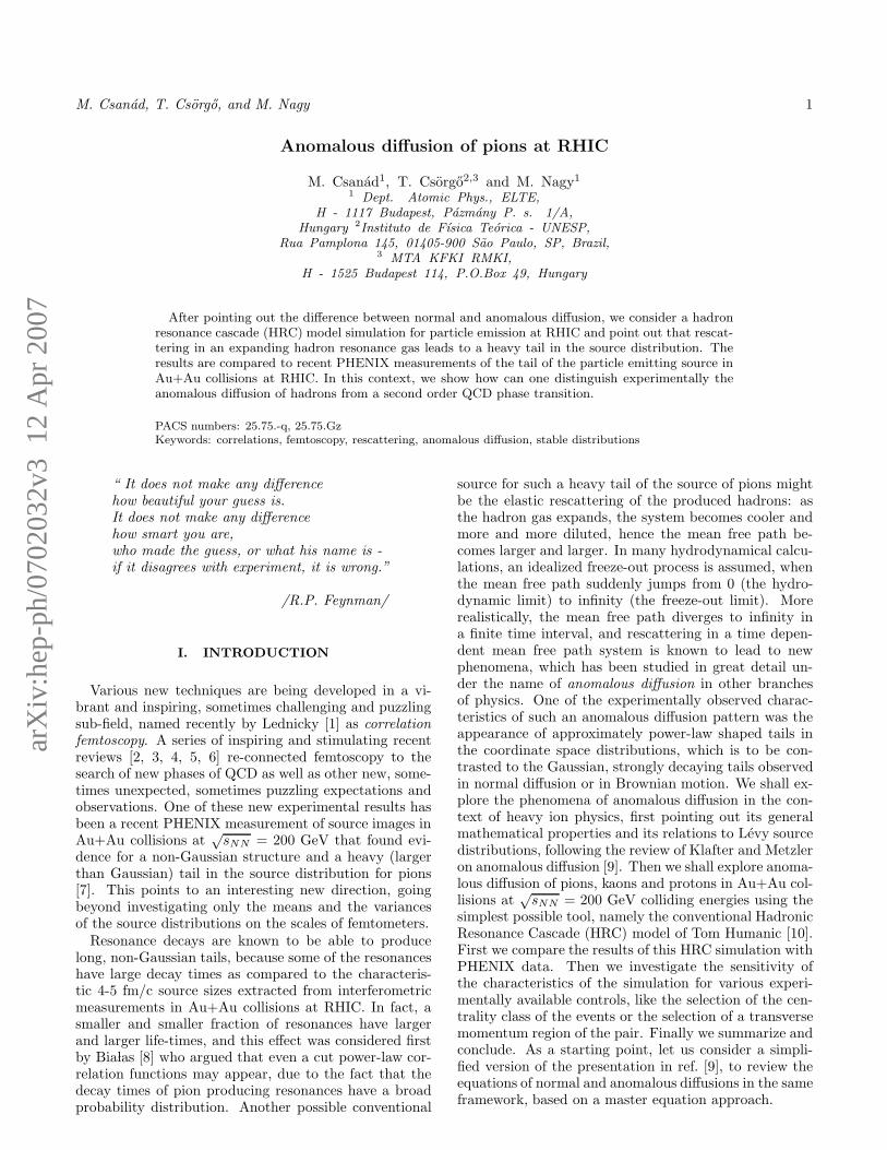
The difference between normal and anomalous diffu-sion is illustrated in Fig. 1, reproduced from ref. [9].

Although the mean displacement or the variance ofthese distributions might diverge, one additional step inthe anomalous diffusion does not change the limiting be-havior of the process.

It is also interesting to note that the tail of anomalousdiffusions has a power-law structure in coordinate space,S(r) ∝ r−(d+α) for r ≫ R, where d is the number ofspatial dimensions (d = 3 in our world), and α is the sameLevy index of stability as before. This asymptotics isyet another important property of the Levy stable sourcedistributions.

Nature often violates Gaussian universality, mirroredin experimental results which do not follow Gaussian pre-dictions [9]. The evidence for a non-Gaussian behavior inmultivariate and univariate source distributions has beenobserved recently also in high energy heavy ion collisions.In fact, the first observation of a non-Gaussian corre-lation function in Au+Au collisions at RHIC has beenmade by the STAR collaboration that utilized an Edge-worth expansion [16] and quantified the deviation fromthe Gaussian structure of the particle emitting source interms of non-vanishing fourth order cumulant momentsof the squared Fourier-transformed source distribution.More recently, the PHENIX Collaboration has appliedthe imaging method of Brown and Danielewicz [17] toreconstruct the two-particle relative coordinate distribu-tion [7]. In this paper, PHENIX observed a clear de-

FIG. 1: Simple illustration of the qualitative properties ofnormal diffusion (bottom) and anomalous diffusion (top). Inthe latter case, large jumps separate various more local partsof the trajectory. The size of the covered region is larger incase of the anomalous diffusion than in case of the Gaussian,normal diffusion. From ref. [9].

viation from a Gaussian structure, and pointed to theappearance of a heavy tail in the two-particle relativecoordinate distribution. In the subsequent part of thismanuscript, we investigate if these PHENIX source func-tion data can be reproduced with the help of Monte-Carlomodels that incorporate the concept of anomalous diffu-sion and that are able to describe the more standardobservable like single particle spectra and the three di-mensional Gaussian fit parameters, Rside, Rout and Rlong

of the measured two-pion correlation functions in highenergy heavy ion collisions.

V. MONTE-CARLO SIMULATIONS OF

ANOMALOUS DIFFUSION OF PIONS

Heavy ion collisions produce thousands of particles ina single high energy nucleus-nucleus collision. The bulkof the particle production, i.e. the momentum distribu-tion and the correlation patterns of 99 % of the particlesare best described by hydrodynamical, or hydrodynam-ically inspired models, see ref. [3] for a recent review.Now we are interested in the tails of particle production,which might indicate a deviation from the hydrodynam-ical behavior. Hence our attention is turned to Monte-Carlo (MC) simulations. Two Monte-Carlo models, theHadronic (or Humanic) Resonance Cascade Model [18],


(HRC) and the AMPT model of Zhang, Ko, Li andLin [19] have also demonstrated [10, 20, 21] their abil-ity to describe single particle spectra, elliptic flow, andHBT correlation measurements in Au+Au collisions with√sNN = 130 and 200 GeV at RHIC.

A. Selection criteria - comparison with data

The selection of the MC model was based on the follow-ing criteria. We looked for a conventional hadronic cas-cade model that describes single particle spectra, ellipticflow data, and HBT data (without any puzzles), henceyields a good description of the hadronic final state, i.e.it yields an acceptable model of S(r).

It also has to be well documented and easy to use, hasto work at CERN SPS as well as at RHIC energies, con-tain the most important short and long lived resonancese.g. ω, η and η′ (hence can be used as a realistic modelfor halo that appears from the decay products of theselong-lived resonances). It is important to require thatthe simulation takes into account the rescattering amongthe hadrons due to possible development of a power-lawtail from the anomalous diffusion, discussed in the earliersections.

Finally we utilized the Hadronic RescatteringModel [18], as it satisfied all the criteria listed above.We expect that similar results are obtained with theAMPT model, but we did not yet investigated thepredictions of this code in detail. The AMPT modelis a multi-phase transport model, while the HRC is asimpler hadronic resonance cascade. When looking fornew effects related to the anomalous diffusion in a timedependent mean free path environment, we have optedfor the simplest possible choice - so that the resultsthen can be uniquely related to the hadronic final stateeffects.

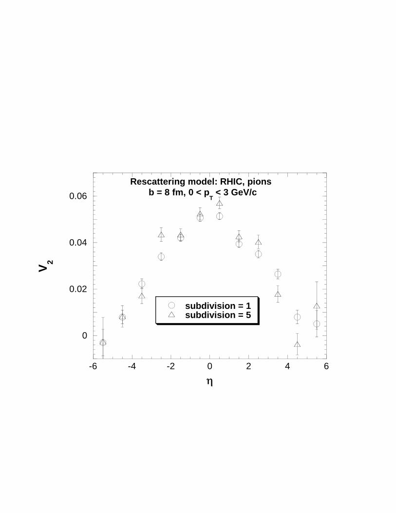
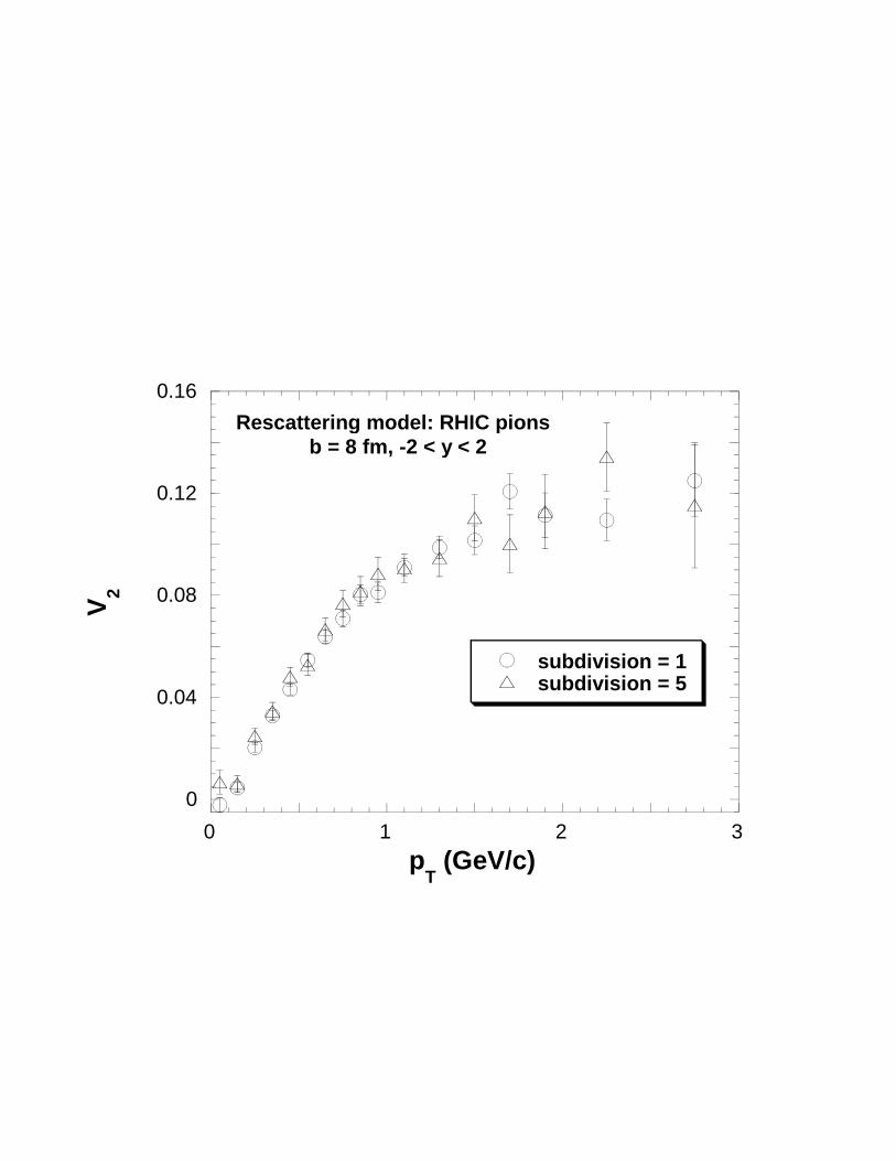
B. Self-consistency criteria - subdivision test

The self-consistency check of subdivision invariance isbased on the invariance of the Boltzmann equation, thebasis of the Monte Carlo particle-scattering calculations,for a simultaneous decrease of the scattering cross sec-tions by some factor l, and an increase of the particledensity by the same factor of l[22]. As l becomes suf-ficiently large, non-causal artifacts become insignificant.The HRC rescattering calculations have been tested bycomparing pion observables for no-subdivision, i.e. l = 1,with subdivision of l = 5. Descriptions of how the ob-servables are extracted from the rescattering calculationare given elsewhere [20].

All calculations were carried out for an impact parame-ter of 8 fm, to simulate semi-central collisions, that resultin significant elliptic flow. Such HRC results [10] repro-duced reasonably well the RHIC data on the correspond-ing observables in Au+Au collisions at

√sNN = 200

0.001

0.1

10

1000

0 1 2 3 4 5

Rescattering model: RHIC, pionsb = 8 fm, -2 < y < 2

subdivision = 1subdivision = 5(1

/pT)

dN

/dp

T (

arb

. un

its)

pT (GeV/c)

FIG. 2: Pion pt distributions for l = 1 and l = 5, from ref. [10].The insensitivity of the transverse momentum distribution tothe number of subdivisions indicates that the scaling proper-ties of the transport equations are satisfied by the HRC code.Similar subdivision tests are satisfied by the HRC code forthe elliptic flow as a function of the transverse momentumv2(pt), the elliptic flow as a function of the longitudinal an-gular variable η as v2(η), see ref. [10] for further details.

GeV. Thus this HRC code passed not only the test ofreproducing the important global observables, but alsothe subdivision test, which suggests that there are nosignificant programming artifacts, or causality violatingterms in this Monte Carlo simulation code. Fig. 2 (takenfrom ref. [10]) shows a comparisons of the l = 1 andthe l = 5 cases utilizing the HRC model to describe thecharge averaged pion spectra. Similar plots were pub-lished for the HBT radius parameters and the transversemomentum and pseudorapidity η dependence of the el-liptic flow. See ref. [10] for further details and for thecomparison plots with RHIC Au+Au data.

C. Self-consistency criteria - comparison with

exact hydrodynamical results

Motivated by the success of the Buda-Lund parame-terization [23, 24] of the hadronic final state, a searchstarted to find parametric, but time dependent, exact so-lutions of hydrodynamics, that lead to Buda-Lund typeof nearly Gaussian freeze-out distributions. Surprisinglylarge classes of exact, parametric solutions of hydrody-namics have been recently found this way, both in thenon-relativistic [25, 26, 27] as well as in the relativistic[28, 29, 30, 31, 32, 33] kinematic domain.

These generalized, Buda-Lund type parametric, hydro-dynamical calculations have a built-in self-quenching ef-fect, as analyzed in detail in ref. [27]. For example, allthe HBT radii stop to evolve in time, they approach adirection independent constant, and expansion velocities


10 20 30 40 50 60 70t [fm/c]

1

2

3

4

Rx, Ry, Rz [fm]

10 20 30 40 50 60 70t [fm/c]

10

20

30

40

50

60

70

X [fm], Y [fm], Z [fm]

10 20 30 40 50 60 70t [fm/c]

200

400

600

800

Tx, Ty, Tz [MeV]

10 20 30 40 50 60 70t [fm/c]

0.2

0.4

0.6

0.8

1

Vx, Vy, Vz

FIG. 3: Time evolution of an expanding ellipsoid with Gaus-sian density profile and homogeneous temperature profile inBuda-Lund type of exact solutions of non-relativistic hydro-dynamics. (X, Y, Z) stand for the principal axis of this ex-panding ellipsoid, after an initial acceleration, these scalesevolve linearly with time (top). The corresponding HBT radii,(Rx, Ry , Rz) approach a direction independent constant (be-low top). The expansion velocities of the principal axis ofthe exploding ellipsoid, (Vx, Vy, Vz) tend to direction depen-dent constants (above bottom panel) and similarly, the slopeparameters of the single particle spectra in the principal di-rections, (Tx, Ty, Tz) also tend to direction independent con-stants (bottom panel). Based on ref. [27].

0

0.01

0.02

0.03

0.04

0.05

0.06

0.07

V2

1

2

3

4

5

6

rad

ius

par

amet

er (

fm)

RT Side

RT Out

RL

250

300

350

400

450

0 5 10 15 20 25

slo

pe

par

amet

er (

MeV

/c)

time (fm/c)

ππππ

K

N

FIG. 4: Time evolution of v2, HBT, and mT slope parametersfrom HRC for RHIC Au+Au, from ref [10]. The HRC codeshows the same self-quenching properties as the Buda-Lundtype of exact solutions of non-relativistic hydrodynamics.

tend to direction dependent constants, although the sys-tem keeps on expanding (via rescattering process or hy-drodynamical evolution). Elliptic flow also freezes out atthe same time when the spectra (slopes) stop to evolve intime. These general, qualitative properties of exact para-metric hydrodynamic solutions are illustrated in Fig. 3.In ref. [27] we have shown that this self-quenching is ageneral property of a large class of exact analytic hydro-dynamic solutions, which is independent of the particularinitial conditions - a beautiful exact result. This propertyof the exact non-relativistic ellipsoidal hydrodynamic so-lutions is beautifully reproduced in the Hadronic Reso-nance Model, as shown on Fig. 4.


D. More than hydro - tails of particle production

As summarized above the HRC resonance cascademodel describes well the observables in heavy ion col-lisions at both CERN SPS and at RHIC energies, and itpasses the subdivision test, and yields such a time evo-lution of the observables, which is similar to the analyti-cally obtained, exact hydrodynamical asymptotic behav-ior of these observables. So HRC looks to be a reliablemodel for the production of the bulk of the particles. Inthe subsequent part, we investigate if the HRC model isable to describe also the tails of the particle productionin

√sNN = 200 GeV Au+Au collisions.

It turns out that this conventional hadronic cascademodel HRC has a built-in adaptive bin size in the timedirection, hence there is no built-in cutoff time scale inthe code. HRC also contains the cascading of the mostabundant hadrons: ρ, ∆, K∗, ω, η, η′, φ and Λ, but it ne-glects electrical charge. Therefore we see that this HRCmodel implements rescattering in a time dependent meanfree path system, and in the previous section we haveshown that under certain conditions this corresponds toa random Levy walk and is signaled by power-law tailsin the source distribution. Let’s see whether the HRCsimulation results confirm such an expectation or not.

VI. DETAILED HRC SIMULATION RESULTS

We generated 48 events with b=4.45 fm and 5730events with 12.5 fm corresponding to the 0-20% and 50-90% centrality classes of PHENIX events. The gener-ated events have average multiplicities of 3400 and 38particles, respectively. The mean impact parameter val-ues suiting the two centralities were determined from aGlauber calculation as in ref. [34].

We made cuts on the data sample similar to the onesin the PHENIX imaging paper [7]:

• 0-20% and 0.2 GeV/c < pt < 0.36 GeV/c,

• 0-20% and 0.48 GeV/c < pt < 0.6 GeV/c,

• 40-90% and 0.2 GeV/c < pt < 0.4 GeV/c,

in addition to the PHENIX geometry cut of −0.5 < y <0.5.

The resulting plots are shown in Figs. 5-22. The com-plete source function is decomposed to different compo-nents, i.e. the S(r) distributions created from pairs withboth pions being

• primordial or decay products of resonances thathave a lifetime less than 20 fm/c; this means heredirect pions ρ, ∆, K∗ decay products, referred toas core, or c pions;

• decay products of an ω

• decay products of resonances that have a lifetimegreater than 25 fm/c; in HRC: Λ, Φ, η, η′, referredto as halo or h pions.

One of the pions in a pair is from one above category, andthe other may be from another one: so in this study wedistinguish (c, c), (c, ω), (c, h), (ω, ω), (ω, h) and (h, h)type of possible combinations.

A. HRC simulations and PHENIX data

In this subsection we compare the HRC model calcu-lations with experimental data from [7]. The kinematiccuts correspond to Figs. 1a,b and Fig.2 of ref. [7].

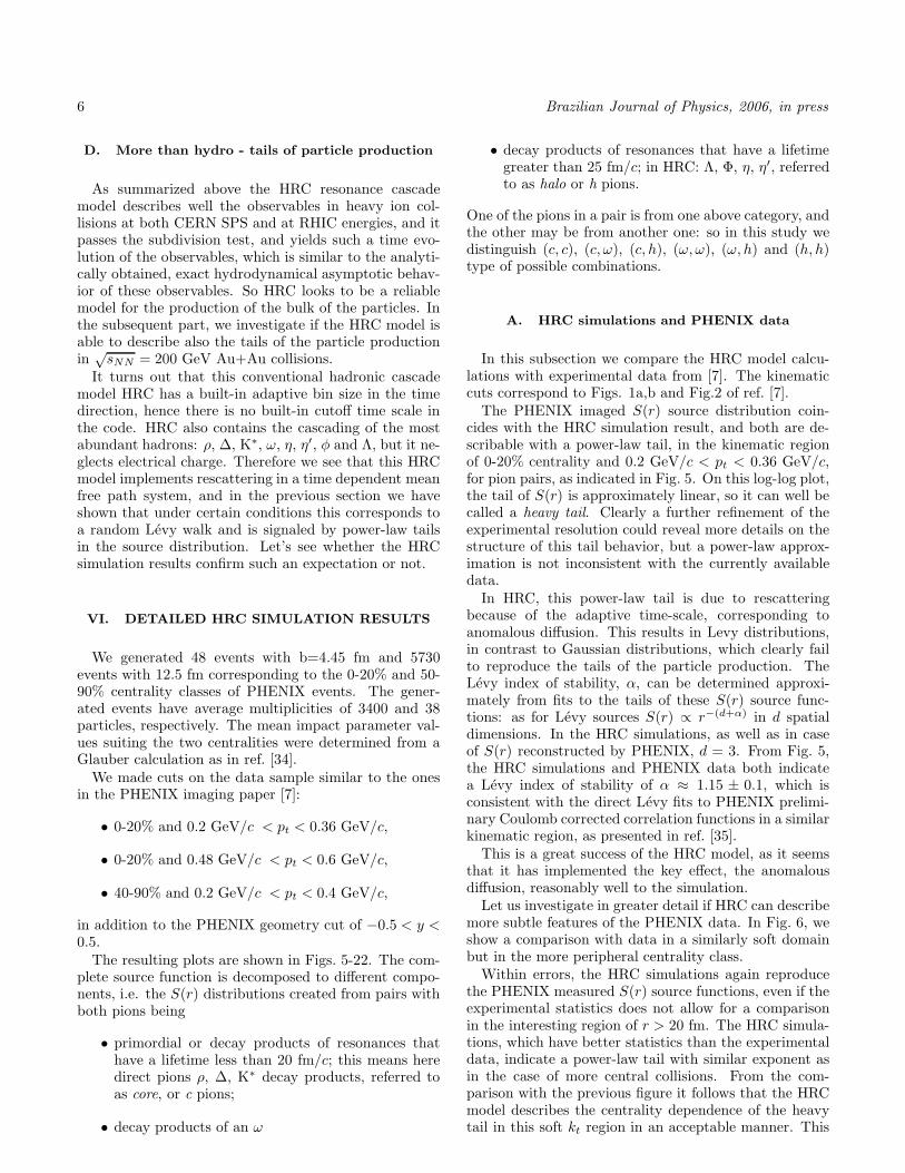
The PHENIX imaged S(r) source distribution coin-cides with the HRC simulation result, and both are de-scribable with a power-law tail, in the kinematic regionof 0-20% centrality and 0.2 GeV/c < pt < 0.36 GeV/c,for pion pairs, as indicated in Fig. 5. On this log-log plot,the tail of S(r) is approximately linear, so it can well becalled a heavy tail. Clearly a further refinement of theexperimental resolution could reveal more details on thestructure of this tail behavior, but a power-law approx-imation is not inconsistent with the currently availabledata.

In HRC, this power-law tail is due to rescatteringbecause of the adaptive time-scale, corresponding toanomalous diffusion. This results in Levy distributions,in contrast to Gaussian distributions, which clearly failto reproduce the tails of the particle production. TheLevy index of stability, α, can be determined approxi-mately from fits to the tails of these S(r) source func-tions: as for Levy sources S(r) ∝ r−(d+α) in d spatialdimensions. In the HRC simulations, as well as in caseof S(r) reconstructed by PHENIX, d = 3. From Fig. 5,the HRC simulations and PHENIX data both indicatea Levy index of stability of α ≈ 1.15 ± 0.1, which isconsistent with the direct Levy fits to PHENIX prelimi-nary Coulomb corrected correlation functions in a similarkinematic region, as presented in ref. [35].

This is a great success of the HRC model, as it seemsthat it has implemented the key effect, the anomalousdiffusion, reasonably well to the simulation.

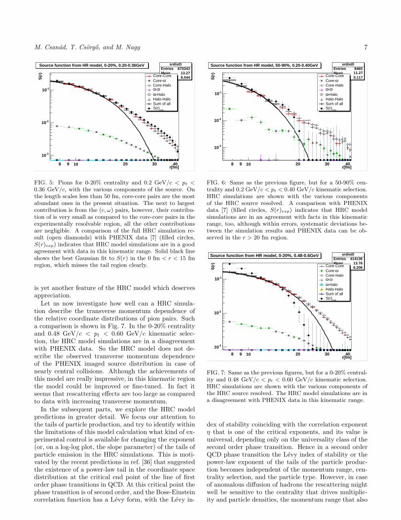
Let us investigate in greater detail if HRC can describemore subtle features of the PHENIX data. In Fig. 6, weshow a comparison with data in a similarly soft domainbut in the more peripheral centrality class.

Within errors, the HRC simulations again reproducethe PHENIX measured S(r) source functions, even if theexperimental statistics does not allow for a comparisonin the interesting region of r > 20 fm. The HRC simula-tions, which have better statistics than the experimentaldata, indicate a power-law tail with similar exponent asin the case of more central collisions. From the com-parison with the previous figure it follows that the HRCmodel describes the centrality dependence of the heavytail in this soft kt region in an acceptable manner. This


r[fm]8 9 10 20 30 40

S(r

)

-310

-210

-110

Source function from HR model, 0-20%, 0.20-0.36GeV srdist0Entries 670343Mean 13.27RMS 6.044

srdist0Entries 670343Mean 13.27RMS 6.044Core-CoreωCore-

Core-Haloω-ω

-HaloωHalo-HaloSum of all

expS(r)

Source function from HR model, 0-20%, 0.20-0.36GeV

FIG. 5: Pions for 0-20% centrality and 0.2 GeV/c < pt <0.36 GeV/c, with the various components of the source. Onthe length scales less than 50 fm, core-core pairs are the mostabundant ones in the present situation. The next to largestcontribution is from the (c, ω) pairs, however, their contribu-tion of is very small as compared to the core-core pairs in theexperimentally resolvable region, all the other contributionsare negligible. A comparison of the full HRC simulation re-sult (open diamonds) with PHENIX data [7] (filled circles,S(r)exp) indicates that HRC model simulations are in a goodagreement with data in this kinematic range. Solid black lineshows the best Gaussian fit to S(r) in the 0 fm < r < 15 fmregion, which misses the tail region clearly.

is yet another feature of the HRC model which deservesappreciation.

Let us now investigate how well can a HRC simula-tion describe the transverse momentum dependence ofthe relative coordinate distributions of pion pairs. Sucha comparison is shown in Fig. 7. In the 0-20% centralityand 0.48 GeV/c < pt < 0.60 GeV/c kinematic selec-tion, the HRC model simulations are in a disagreementwith PHENIX data. So the HRC model does not de-scribe the observed transverse momentum dependenceof the PHENIX imaged source distribution in case ofnearly central collisions. Although the achievements ofthis model are really impressive, in this kinematic regionthe model could be improved or fine-tuned. In fact itseems that rescattering effects are too large as comparedto data with increasing transverse momentum.

In the subsequent parts, we explore the HRC modelpredictions in greater detail. We focus our attention tothe tails of particle production, and try to identify withinthe limitations of this model calculation what kind of ex-perimental control is available for changing the exponent(or, on a log-log plot, the slope parameter) of the tails ofparticle emission in the HRC simulations. This is moti-vated by the recent predictions in ref. [36] that suggestedthe existence of a power-law tail in the coordinate spacedistribution at the critical end point of the line of firstorder phase transitions in QCD. At this critical point thephase transition is of second order, and the Bose-Einsteincorrelation function has a Levy form, with the Levy in-

r[fm]8 9 10 20 30 40

S(r

)

-310

-210

-110



Core-Haloω-ω


expS(r)


FIG. 6: Same as the previous figure, but for a 50-90% cen-trality and 0.2 GeV/c < pt < 0.40 GeV/c kinematic selection.HRC simulations are shown with the various componentsof the HRC source resolved. A comparison with PHENIXdata [7] (filled circles, S(r)exp) indicates that HRC modelsimulations are in an agreement with facts in this kinematicrange, too, although within errors, systematic deviations be-tween the simulation results and PHENIX data can be ob-served in the r > 20 fm region.

r[fm]8 9 10 20 30 40

S(r

)

-310

-210

-110



Core-Haloω-ω


expS(r)


FIG. 7: Same as the previous figures, but for a 0-20% central-ity and 0.48 GeV/c < pt < 0.60 GeV/c kinematic selection.HRC simulations are shown with the various components ofthe HRC source resolved. The HRC model simulations are ina disagreement with PHENIX data in this kinematic range.

dex of stability coinciding with the correlation exponentη that is one of the critical exponents, and its value isuniversal, depending only on the universality class of thesecond order phase transition. Hence in a second orderQCD phase transition the Levy index of stability or thepower-law exponent of the tails of the particle produc-tion becomes independent of the momentum range, cen-trality selection, and the particle type. However, in caseof anomalous diffusion of hadrons the rescattering mightwell be sensitive to the centrality that drives multiplic-ity and particle densities, the momentum range that also


r[fm]10

S(r

)

-310

-210

-110

1

Source function sradiusEntries 99957Mean 16.41RMS 8.275

Pions, 0.2-0.4 GeV

centr.: 0-10%

centr.: 10-20%

centr.: 20-30%

centr.: 30-50%

centr.: 50-80%

Source function

FIG. 8: Source distribution of HRC simulated pion pairs with0.2 GeV/c < pt < 0.4 GeV/c for various centrality classes.

r[fm]10

S(r

)

-310

-210

-110

1


Kaons, 0.2-0.4 GeV

centr.: 0-10%

centr.: 10-20%

centr.: 20-30%

centr.: 30-50%

centr.: 50-80%

Source function

FIG. 9: Source distribution of HRC simulated pion pairs with0.5 GeV/c < pt < 1.0 GeV/c for various centrality classes.

influences how many particles take part in the rescatter-ing process and also the particle type, as the number ofrescatterings is expected to depend on the particle crosssections.

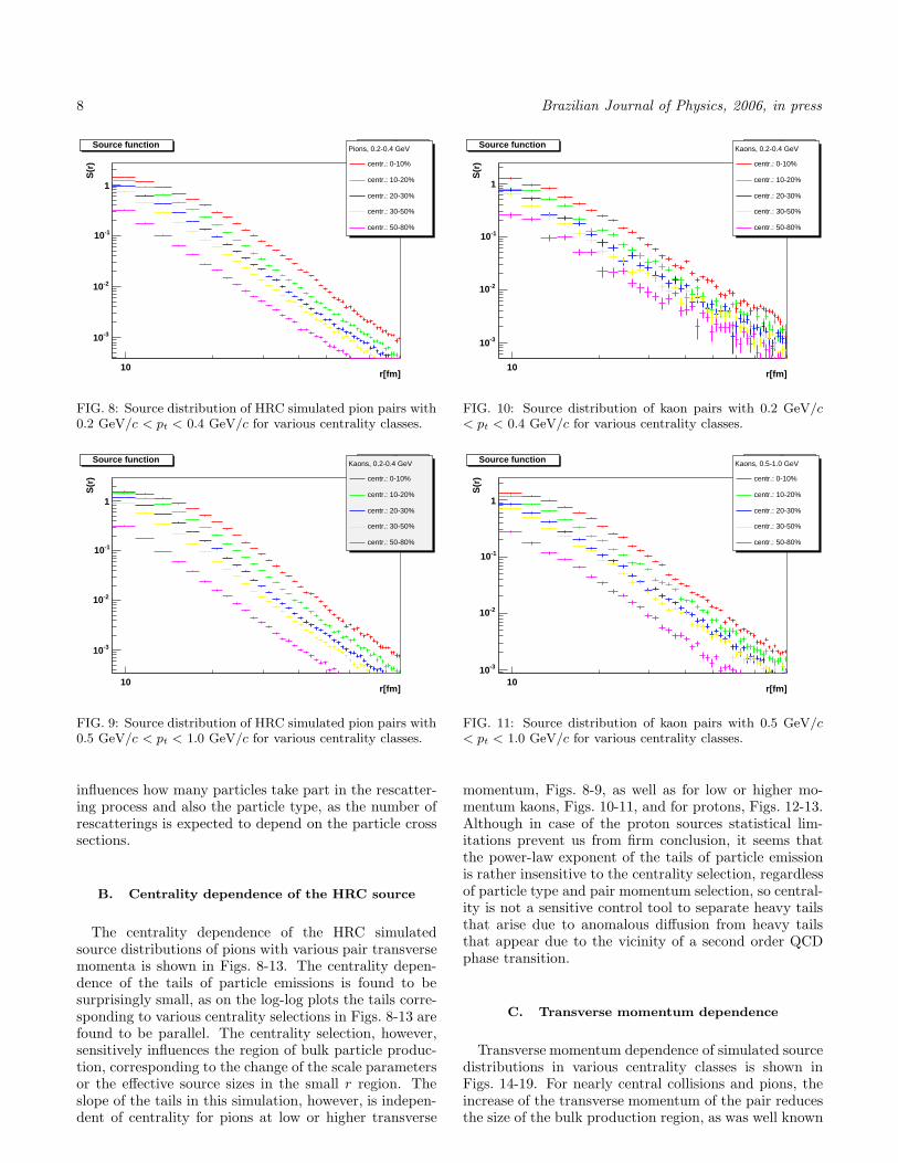
B. Centrality dependence of the HRC source

The centrality dependence of the HRC simulatedsource distributions of pions with various pair transversemomenta is shown in Figs. 8-13. The centrality depen-dence of the tails of particle emissions is found to besurprisingly small, as on the log-log plots the tails corre-sponding to various centrality selections in Figs. 8-13 arefound to be parallel. The centrality selection, however,sensitively influences the region of bulk particle produc-tion, corresponding to the change of the scale parametersor the effective source sizes in the small r region. Theslope of the tails in this simulation, however, is indepen-dent of centrality for pions at low or higher transverse

r[fm]10

S(r

)

-310

-210

-110

1


Kaons, 0.2-0.4 GeV

centr.: 0-10%

centr.: 10-20%

centr.: 20-30%

centr.: 30-50%

centr.: 50-80%

Source function

FIG. 10: Source distribution of kaon pairs with 0.2 GeV/c< pt < 0.4 GeV/c for various centrality classes.

r[fm]10

S(r

)

-310

-210

-110

1


Kaons, 0.5-1.0 GeV

centr.: 0-10%

centr.: 10-20%

centr.: 20-30%

centr.: 30-50%

centr.: 50-80%

Source function

FIG. 11: Source distribution of kaon pairs with 0.5 GeV/c< pt < 1.0 GeV/c for various centrality classes.

momentum, Figs. 8-9, as well as for low or higher mo-mentum kaons, Figs. 10-11, and for protons, Figs. 12-13.Although in case of the proton sources statistical lim-itations prevent us from firm conclusion, it seems thatthe power-law exponent of the tails of particle emissionis rather insensitive to the centrality selection, regardlessof particle type and pair momentum selection, so central-ity is not a sensitive control tool to separate heavy tailsthat arise due to anomalous diffusion from heavy tailsthat appear due to the vicinity of a second order QCDphase transition.

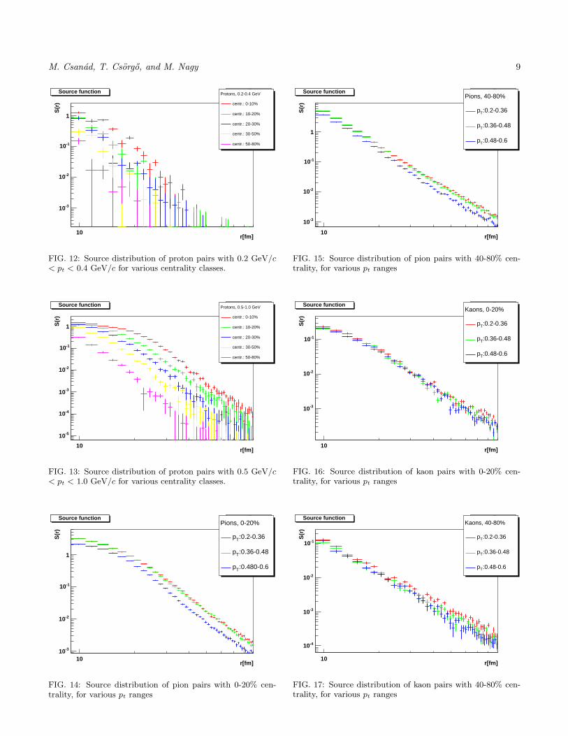
C. Transverse momentum dependence

Transverse momentum dependence of simulated sourcedistributions in various centrality classes is shown inFigs. 14-19. For nearly central collisions and pions, theincrease of the transverse momentum of the pair reducesthe size of the bulk production region, as was well known


r[fm]10

S(r

)

-310

-210

-110

1


Protons, 0.2-0.4 GeV

centr.: 0-10%

centr.: 10-20%

centr.: 20-30%

centr.: 30-50%

centr.: 50-80%

Source function

FIG. 12: Source distribution of proton pairs with 0.2 GeV/c< pt < 0.4 GeV/c for various centrality classes.

r[fm]10

S(r

)

-510

-410

-310

-210

-110

1


Protons, 0.5-1.0 GeV

centr.: 0-10%

centr.: 10-20%

centr.: 20-30%

centr.: 30-50%

centr.: 50-80%

Source function

FIG. 13: Source distribution of proton pairs with 0.5 GeV/c< pt < 1.0 GeV/c for various centrality classes.

r[fm]10

S(r

)

-310

-210

-110

1


Pions, 0-20%

:0.2-0.36Tp

:0.36-0.48Tp

:0.480-0.6Tp

Source function

FIG. 14: Source distribution of pion pairs with 0-20% cen-trality, for various pt ranges

r[fm]10

S(r

)

-310

-210

-110

1


Pions, 40-80%

:0.2-0.36Tp

:0.36-0.48Tp

:0.48-0.6Tp

Source function

FIG. 15: Source distribution of pion pairs with 40-80% cen-trality, for various pt ranges

r[fm]10

S(r

)

-310

-210

-110


Kaons, 0-20%

:0.2-0.36Tp

:0.36-0.48Tp

:0.48-0.6Tp

Source function

FIG. 16: Source distribution of kaon pairs with 0-20% cen-trality, for various pt ranges

r[fm]10

S(r

)

-410

-310

-210

-110


Kaons, 40-80%

:0.2-0.36Tp

:0.36-0.48Tp

:0.48-0.6Tp

Source function

FIG. 17: Source distribution of kaon pairs with 40-80% cen-trality, for various pt ranges


r[fm]10

S(r

)

-410

-310

-210

-110


Protons, 0-20%

:0.2-0.36Tp

:0.36-0.48Tp

:0.48-0.6Tp

Source function

FIG. 18: Source distribution of proton pairs with 0-20% cen-trality, for various pt ranges

from earlier Bose-Einstein correlation measurements andtheoretical explanations, see e.g. refs. [23, 24]. Beingaware of the strong transverse momentum dependencesof the scale parameter R, which is well shown by the HRCsimulation, it is rather surprising, that the shape param-eter of the tail, the Levy index of stability α is remark-ably insensitive to the selected transverse momentum re-gions, which follows from the fact that on the log-log plotthe simulated S(r) tails are parallel to one another, seeFig. 14. The same effect is shown in Fig. 15, in caseof peripheral collisions. For kaons, the evolution of thesource function is less apparent in the same transversemomentum regions, this is due to the fact that the effec-tive radius parameters, the scales in analytic calculationslike of refs. [23, 24], are found to be predominantly de-

pending on the transverse mass, mt =√

m2 + p2t of the

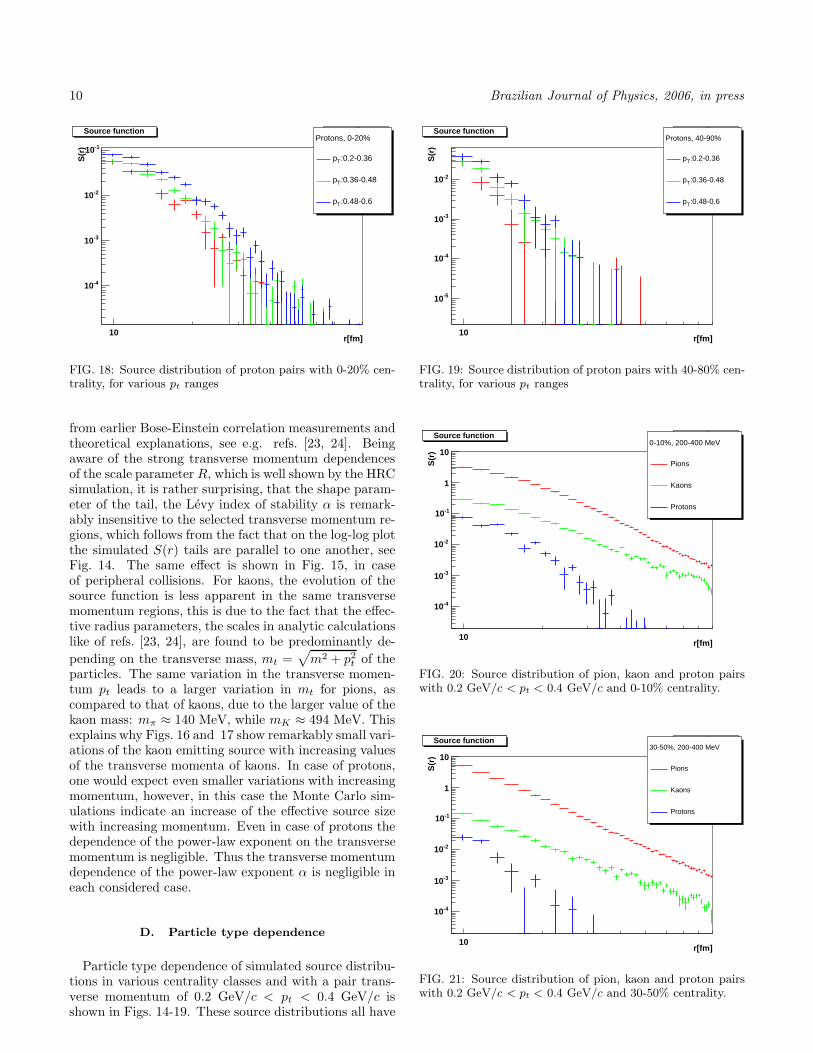
particles. The same variation in the transverse momen-tum pt leads to a larger variation in mt for pions, ascompared to that of kaons, due to the larger value of thekaon mass: mπ ≈ 140 MeV, while mK ≈ 494 MeV. Thisexplains why Figs. 16 and 17 show remarkably small vari-ations of the kaon emitting source with increasing valuesof the transverse momenta of kaons. In case of protons,one would expect even smaller variations with increasingmomentum, however, in this case the Monte Carlo sim-ulations indicate an increase of the effective source sizewith increasing momentum. Even in case of protons thedependence of the power-law exponent on the transversemomentum is negligible. Thus the transverse momentumdependence of the power-law exponent α is negligible ineach considered case.

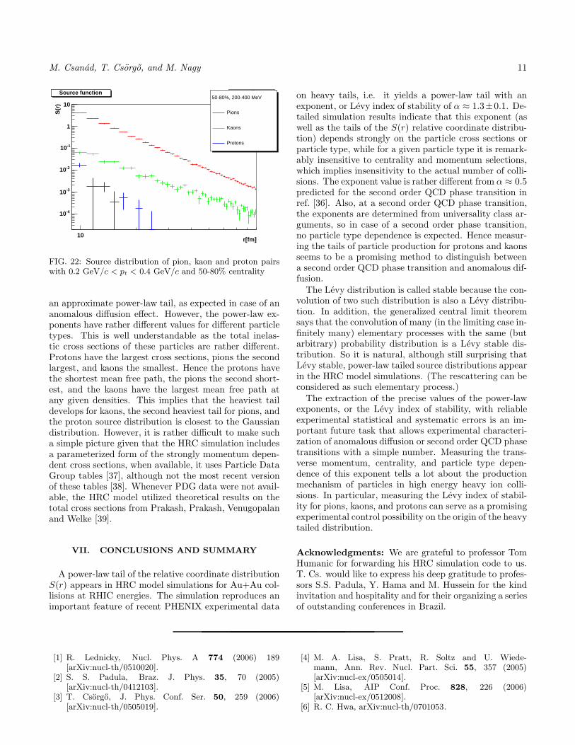
D. Particle type dependence

Particle type dependence of simulated source distribu-tions in various centrality classes and with a pair trans-verse momentum of 0.2 GeV/c < pt < 0.4 GeV/c isshown in Figs. 14-19. These source distributions all have

r[fm]10

S(r

)

-510

-410

-310

-210


Protons, 40-90%

:0.2-0.36Tp

:0.36-0.48Tp

:0.48-0.6Tp

Source function

FIG. 19: Source distribution of proton pairs with 40-80% cen-trality, for various pt ranges

r[fm]10

S(r

)

-410

-310

-210

-110

1

10


0-10%, 200-400 MeV

Pions

Kaons

Protons

Source function

FIG. 20: Source distribution of pion, kaon and proton pairswith 0.2 GeV/c < pt < 0.4 GeV/c and 0-10% centrality.

r[fm]10

S(r

)

-410

-310

-210

-110

1

10


30-50%, 200-400 MeV

Pions

Kaons

Protons

Source function

FIG. 21: Source distribution of pion, kaon and proton pairswith 0.2 GeV/c < pt < 0.4 GeV/c and 30-50% centrality.


r[fm]10

S(r

)

-410

-310

-210

-110

1

10


50-80%, 200-400 MeV

Pions

Kaons

Protons

Source function

FIG. 22: Source distribution of pion, kaon and proton pairswith 0.2 GeV/c < pt < 0.4 GeV/c and 50-80% centrality

an approximate power-law tail, as expected in case of ananomalous diffusion effect. However, the power-law ex-ponents have rather different values for different particletypes. This is well understandable as the total inelas-tic cross sections of these particles are rather different.Protons have the largest cross sections, pions the secondlargest, and kaons the smallest. Hence the protons havethe shortest mean free path, the pions the second short-est, and the kaons have the largest mean free path atany given densities. This implies that the heaviest taildevelops for kaons, the second heaviest tail for pions, andthe proton source distribution is closest to the Gaussiandistribution. However, it is rather difficult to make sucha simple picture given that the HRC simulation includesa parameterized form of the strongly momentum depen-dent cross sections, when available, it uses Particle DataGroup tables [37], although not the most recent versionof these tables [38]. Whenever PDG data were not avail-able, the HRC model utilized theoretical results on thetotal cross sections from Prakash, Prakash, Venugopalanand Welke [39].

VII. CONCLUSIONS AND SUMMARY

A power-law tail of the relative coordinate distributionS(r) appears in HRC model simulations for Au+Au col-lisions at RHIC energies. The simulation reproduces animportant feature of recent PHENIX experimental data

on heavy tails, i.e. it yields a power-law tail with anexponent, or Levy index of stability of α ≈ 1.3±0.1. De-tailed simulation results indicate that this exponent (aswell as the tails of the S(r) relative coordinate distribu-tion) depends strongly on the particle cross sections orparticle type, while for a given particle type it is remark-ably insensitive to centrality and momentum selections,which implies insensitivity to the actual number of colli-sions. The exponent value is rather different from α ≈ 0.5predicted for the second order QCD phase transition inref. [36]. Also, at a second order QCD phase transition,the exponents are determined from universality class ar-guments, so in case of a second order phase transition,no particle type dependence is expected. Hence measur-ing the tails of particle production for protons and kaonsseems to be a promising method to distinguish betweena second order QCD phase transition and anomalous dif-fusion.

The Levy distribution is called stable because the con-volution of two such distribution is also a Levy distribu-tion. In addition, the generalized central limit theoremsays that the convolution of many (in the limiting case in-finitely many) elementary processes with the same (butarbitrary) probability distribution is a Levy stable dis-tribution. So it is natural, although still surprising thatLevy stable, power-law tailed source distributions appearin the HRC model simulations. (The rescattering can beconsidered as such elementary process.)

The extraction of the precise values of the power-lawexponents, or the Levy index of stability, with reliableexperimental statistical and systematic errors is an im-portant future task that allows experimental characteri-zation of anomalous diffusion or second order QCD phasetransitions with a simple number. Measuring the trans-verse momentum, centrality, and particle type depen-dence of this exponent tells a lot about the productionmechanism of particles in high energy heavy ion colli-sions. In particular, measuring the Levy index of stabil-ity for pions, kaons, and protons can serve as a promisingexperimental control possibility on the origin of the heavytailed distribution.

Acknowledgments: We are grateful to professor TomHumanic for forwarding his HRC simulation code to us.T. Cs. would like to express his deep gratitude to profes-sors S.S. Padula, Y. Hama and M. Hussein for the kindinvitation and hospitality and for their organizing a seriesof outstanding conferences in Brazil.

[1] R. Lednicky, Nucl. Phys. A 774 (2006) 189[arXiv:nucl-th/0510020].

[2] S. S. Padula, Braz. J. Phys. 35, 70 (2005)[arXiv:nucl-th/0412103].

[3] T. Csorgo, J. Phys. Conf. Ser. 50, 259 (2006)[arXiv:nucl-th/0505019].

[4] M. A. Lisa, S. Pratt, R. Soltz and U. Wiede-mann, Ann. Rev. Nucl. Part. Sci. 55, 357 (2005)[arXiv:nucl-ex/0505014].

[5] M. Lisa, AIP Conf. Proc. 828, 226 (2006)[arXiv:nucl-ex/0512008].

[6] R. C. Hwa, arXiv:nucl-th/0701053.

http://arXiv.org/abs/nucl-th/0510020



http://arXiv.org/abs/nucl-ex/0505014




[7] S. S. Adler et al. [PHENIX Collaboration],arXiv:nucl-ex/0605032.

[8] A. Bia las, Acta Phys. Polon. B 23, 561 (1992).[9] R. Metzler, J. Klafter, Physics Reports 339 (2000) 1-77

[10] T. J. Humanic, Int. J. Mod. Phys. E 15, 197 (2006)[arXiv:nucl-th/0510049].

[11] V. V. Uchaikin and V. M. Zolotarev, “Chance and Sta-bility, Stable Distributions and Their Applications”, VSPScience,1999, ISBN: 90-6764-301-7, 596 pp.

[12] V. M. Zolotarev, “One-dimensional Stable Distribu-tions”, Am. Math. Soc. Transl. of Math. Monographs,vol. 65, Providence, R.I. (Transl. of the original 1983Russian)

[13] J. P. Nolan, Stable Distributions: Models for HeavyTailed Datahttp://academic2.american.edu/˜jpnolan/stable/CHAP1.PDF

[14] Nolan, J. P. Stable Distributions: Models for HeavyTailed Data. Boston, MA: Birkhuser, 2005

[15] T. Csorgo, S. Hegyi and W. A. Zajc, Eur. Phys. J. C 36,67 (2004) [arXiv:nucl-th/0310042].

[16] J. Adams et al. [STAR Collaboration], Phys. Rev. C 71,044906 (2005) [arXiv:nucl-ex/0411036].

[17] D. A. Brown and P. Danielewicz, Phys. Lett. B 398, 252(1997) [arXiv:nucl-th/9701010].

[18] T. J. Humanic, arXiv:nucl-th/0301055.[19] B. Zhang, C. M. Ko, B. A. Li and Z. w. Lin, Phys. Rev.

C 61, 067901 (2000) [arXiv:nucl-th/9907017].[20] T. J. Humanic, arXiv:nucl-th/0205053.[21] C. M. Ko, Z. W. Lin and S. Pal, Heavy Ion Phys. 17,

219 (2003) [arXiv:nucl-th/0205056].[22] B. Zhang, M. Gyulassy and Y. Pang, Phys. Rev. C 58,

1175 (1998)[23] T. Csorgo and B. Lorstad, Phys. Rev. C 54, 1390 (1996)

[arXiv:hep-ph/9509213].[24] M. Csanad, T. Csorgo and B. Lorstad, Nucl. Phys. A

742, 80 (2004) [arXiv:nucl-th/0310040].[25] T. Csorgo, Acta Phys. Polon. B 37, 483 (2006)

[arXiv:hep-ph/0111139].[26] T. Csorgo, S. V. Akkelin, Y. Hama, B. Lukacs and

Yu. M. Sinyukov, Phys. Rev. C 67, 034904 (2003)[arXiv:hep-ph/0108067].

[27] T. Csorgo and J. Zimanyi, Heavy Ion Phys. 17, 281(2003) [arXiv:nucl-th/0206051].

[28] T. S. Biro, Phys. Lett. B 474, 21 (2000)[arXiv:nucl-th/9911004].

[29] T. Csorgo, L. P. Csernai, Y. Hama and T. Ko-dama, Heavy Ion Phys. A 21, 73 (2004)[arXiv:nucl-th/0306004].

[30] T. Csorgo, F. Grassi, Y. Hama and T. Kodama, Phys.Lett. B 565, 107 (2003) [arXiv:nucl-th/0305059].

[31] Yu. M. Sinyukov and I. A. Karpenko, Acta Phys.Hung.A25, 141-147 (2006) [arXiv:nucl-th/0506002].

[32] T. Csorgo, M. I. Nagy and M. Csanad,arXiv:nucl-th/0605070.

[33] S. Pratt, arXiv:nucl-th/0612010.[34] S. S. Adler et al. [PHENIX Collaboration], Phys. Rev. C

69, 034910 (2004) [arXiv:nucl-ex/0308006].[35] M. Csanad [PHENIX Collaboration], Nucl. Phys. A 774,

611 (2006) [arXiv:nucl-ex/0509042].[36] T. Csorgo, S. Hegyi, T. Novak and W. A. Zajc, AIP Conf.

Proc. 828, 525 (2006) [arXiv:nucl-th/0512060];T. Csorgo, S. Hegyi, T. Novak and W. A. Zajc, ActaPhys. Polon. B 36, 329 (2005) [arXiv:hep-ph/0412243].

[37] K. Hikasa et al., Particle Data Group, Phys. Rev. D 45

(1992) 83[38] W-M Yao et al., Particle Data Group, J. Phys. G: Nucl.

Part. Phys. 33 (2006) 1-1232[39] M. Prakash, M. Prakash, R. Venugopalan and G. Welke,

Phys. Rept. 227, 321 (1993).



http://academic2.american.edu/








http://arXiv.org/abs/hep-ph/9509213















0

2

4

6

0 0.2 0.4 0.6 0.8 1

Rescattering model: RHIC, pionsb = 8 fm, -2 < y < 2

OORTsideRToutRLong

R (

fm)

pT (GeV/c)

black: subdivision = 1open: subdivision = 5

0

1

OO

0

0.02

0.04

0.06

-6 -4 -2 0 2 4 6

Rescattering model: RHIC, pionsb = 8 fm, 0 < p

T < 3 GeV/c

subdivision = 5subdivision = 1

V2

KK

0

0.04

0.08

0.12

0.16

0 1 2 3

Rescattering model: RHIC pionsb = 8 fm, -2 < y < 2

subdivision = 1subdivision = 5

V2

pT (GeV/c)

Anomalous Diffusion of Pions at RHIC

Documents

Transcript of Anomalous Diffusion of Pions at RHIC