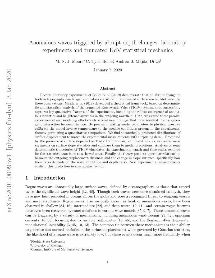
Anomalous waves triggered by abrupt depth changes: laboratory

experiments and truncated KdV statistical mechanics

M. N. J. Moore∗, C. Tyler Bolles†, Andrew J. Majda‡, Di Qi‡

January 7, 2020

Abstract

Recent laboratory experiments of Bolles et al. (2019) demonstrate that an abrupt change inbottom topography can trigger anomalous statistics in randomized surface waves. Motivated bythese observations, Majda et al. (2019) developed a theoretical framework, based on determinis-tic and statistical analysis of the truncated Kortewegde Vries (TKdV) system, that successfullycaptures key qualitative features of the experiments, including the robust emergence of anoma-lous statistics and heightened skewness in the outgoing wavefield. Here, we extend these parallelexperimental and modeling efforts with several new findings that have resulted from a syner-getic interaction between the two. By precisely relating model parameters to physical ones, wecalibrate the model inverse temperature to the specific conditions present in the experiments,thereby permitting a quantitative comparison. We find theoretically predicted distributions ofsurface displacement to match the experimental measurements with surprising detail. Promptedby the presence of surface slope in the TKdV Hamiltonian, we present new experimental mea-surements on surface slope statistics and compare them to model predictions. Analysis of somedeterministic trajectories of TKdV elucidates the experimental length and time scales requiredfor the statistical transition to a skewed state. Finally, the theory predicts a peculiar relationshipbetween the outgoing displacement skewness and the change in slope variance, specifically howtheir ratio depends on the wave amplitude and depth ratio. New experimental measurementsconfirm this prediction in spectacular fashion.

1 Introduction

Rogue waves are abnormally large surface waves, defined by oceanographers as those that exceedtwice the significant wave height [32, 48]. Though such waves were once dismissed as myth, theyhave now been recorded in oceans across the globe and pose a recognized threat to seagoing vesselsand naval structures. Rogue waves, also variously known as freak or anomalous waves, have beenobserved in shallow [34, 16], intermediate [22], and deep water [12, 11], and certain rogue featureshave even been recovered by exact solutions to various wave models [35, 9, 7]. These abnormal wavescan be triggered by a variety of mechanisms, including anomalous wind-forcing [23, 42], opposingcurrents [15, 33], focusing due to variable bathymetry [18, 46], and the Benjamin-Feir deep-watermodulational instability [3, 45, 10, 13]. The common tie between these mechanisms is their abilityto generate non-normal statistics in the surface displacement: when governed by Gaussian statistics,the likelihood of a rogue wave is extremely low, but these events occur much more frequently when

∗Florida State University†University of Michigan‡Courant Institute of Mathematical Sciences

1

arX

iv:2

001.

0099

5v1

[ph

ysic

s.fl

u-dy

n] 3

Jan

202

0

surface statistics deviate from Gaussian. In this way, anomalous waves can be approached from thebroader perspective of turbulent dynamical systems [41, 40, 39, 8, 28, 26, 27, 4, 17, 20].

A recent series of laboratory [5, 43] and numerical investigations [44, 19] have demonstratedthe emergence of anomalous wave statistics from abrupt variations in bottom topography. Sincetopographical variations are strictly one-dimensional, these studies can be viewed as offering a bareminimum set of conditions capable of generating anomalous waves. In particular, the more complexmechanism of focusing by 2D bottom topography is absent. The studies thus offer a paradigmsystem, with emergent anomalous features similar to those seen in more complex systems, but in atractable context that is amenable to analysis.

Our particular focus is the laboratory experiments of Bolles et al. (2019) [5], who demonstratedthe emergence of anomalous statistics from a randomized wave-field encountering an abrupt depthchange (ADC). In these experiments, the incoming wave-field is generated with nearly Gaussianstatistics, and a plexiglass step placed near the middle of the tank creates the depth change. Uponpassing over the step, the wave distribution skews strongly towards positive displacement, withdeviation from Gaussian being most pronounced a short distance downstream of the ADC. Inspiredby these experimental observations, Majda et al. (2019) [29] developed a theoretical frameworkthat accurately captures several key aspects of the anomalous behavior. The theory is based ondeterministic and statistical analysis of the truncated Kortewegde Vries (TKdV) equations, anduses a combination of computational, statistical, and analytical tools. In subsequent work, Majda& Qi (2019) [30] analyzed more severely truncated systems — as low as two interacting modes —that exhibit a statistical phase transition to anomalous statistics and the creation of extreme eventswhile enjoying a more tractable structure. More recently, Qi & Majda (2019) [36] demonstratedthe capability of machine learning strategies to accurately predict these extreme events. Thatwork employs a deep neural network coupled with a judicious choice of the entropy loss functionthat emphasizes the dominant structures of the turbulent field [36]. It should be noted that, inthese studies, extreme events are represented by strong skewness of the wave-field. They occurintermittently and on a relatively frequent basis, which is in contrast to the simpler situation ofisolated, rare events [17].

The purpose of the present manuscript is to provide a more comprehensive treatment of the com-bined experimental and theoretical efforts of Bolles et al. (2019) [5] and Majda et al. (2019) [29, 30].We present a variety of new findings that have resulted from a synergetic interaction between theoryand experiments – a cooperative strategy with a proven record of success [6, 38, 14]. That outline ofthe paper is as follows. In Section 2 we detail the laboratory experiments of Bolles et al. (2019) [5]and summarize previously reported findings on anomalous statistics of the surface displacement.We also present new experimental data on surface slope statistics — a line of inquiry motivated bythe theoretical advancements of Majda et al. (2019) [29], specifically the central role played by theslope in the Hamiltonian structure of TKdV. Section 3 discusses the TKdV theoretical framework,including both the deterministic and the statistical mechanics perspectives. In this section, we fleshout details of the non-dimensionalization, which, for brevity, were only briefly discussed in previouswork. This exercise provides a more precise link between model and experimental parameters, ulti-mately facilitating a closer comparison between the two. We then discuss TKdV as a deterministicdynamical system, approachable from the viewpoint of statistical mechanics. The later perspectiveis based on the Hamiltonian structure and novel ensemble distributions that incorporate canonicaland micro-canonical aspects [1].

Section 4 presents a systematic comparison between experiments and theory, focusing on bothsurface displacement and surface slope. We find the statistical distributions of these two quanti-ties to agree well across experiments and theory. In particular, we find remarkably quantitativeagreement in the displacement statistics. We then examine numerical simulations of the TKdV de-

2

η(x,t)

wave directionpaddle

motor

dampener

step

camera view

φ

180 185 190 195 200 205 210 215 220-1.0

-0.5

0

0.5

1.0Upstream

time (s)

η (c

m)

180 185 190 195 200 205 210 215 220-1.0

-0.5

0

0.5

1.0Downstream

time (s)

η (c

m)

-1.0 -0.5 0 0.5 1.00.01

0.1

1

η (cm)

p(η)

-1.0 -0.5 0 0.5 1.00.01

0.1

1

η (cm)p(η)

(a)

(b) (c)

(d) (e)

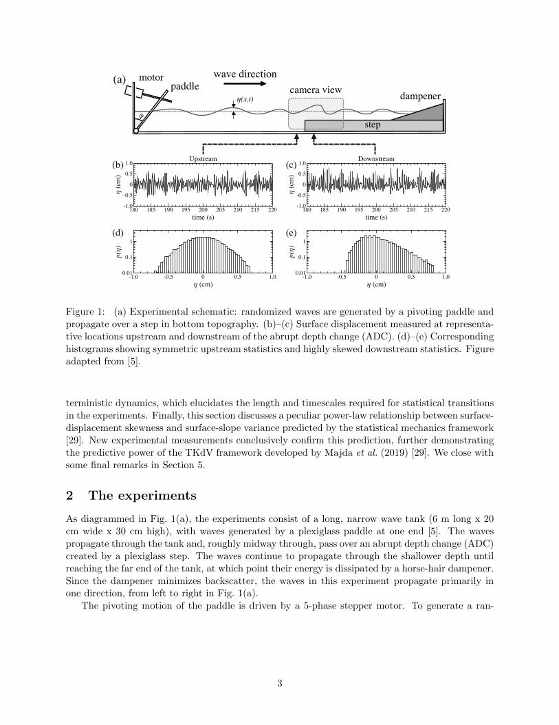
Figure 1: (a) Experimental schematic: randomized waves are generated by a pivoting paddle andpropagate over a step in bottom topography. (b)–(c) Surface displacement measured at representa-tive locations upstream and downstream of the abrupt depth change (ADC). (d)–(e) Correspondinghistograms showing symmetric upstream statistics and highly skewed downstream statistics. Figureadapted from [5].

terministic dynamics, which elucidates the length and timescales required for statistical transitionsin the experiments. Finally, this section discusses a peculiar power-law relationship between surface-displacement skewness and surface-slope variance predicted by the statistical mechanics framework[29]. New experimental measurements conclusively confirm this prediction, further demonstratingthe predictive power of the TKdV framework developed by Majda et al. (2019) [29]. We close withsome final remarks in Section 5.

2 The experiments

As diagrammed in Fig. 1(a), the experiments consist of a long, narrow wave tank (6 m long x 20cm wide x 30 cm high), with waves generated by a plexiglass paddle at one end [5]. The wavespropagate through the tank and, roughly midway through, pass over an abrupt depth change (ADC)created by a plexiglass step. The waves continue to propagate through the shallower depth untilreaching the far end of the tank, at which point their energy is dissipated by a horse-hair dampener.Since the dampener minimizes backscatter, the waves in this experiment propagate primarily inone direction, from left to right in Fig. 1(a).

The pivoting motion of the paddle is driven by a 5-phase stepper motor. To generate a ran-

3

domized wave field, the paddle angle φ is specified by a psuedo-random signal

φ(t) = φ0 + ∆φN∑n=1

an cos(ωnt+ δn) , (1)

an =

√2∆ω

π1/2σωexp

(−(ωn − ω0)2

2σ2ω

), (2)

The angular frequencies are evenly spaced ωn = n∆ω with step size ∆ω = (ω0 + 4σω)/N , where ω0

and σω represent the mean and the bandwidth of ω respectively. As in prior work, all experimentsreported here use the values ω0 = σω = 12.5 rad/s, corresponding to a peak forcing frequency of2 Hz and bandwidth of 2 Hz. The phases δn are uniformly distributed random variables, whichresults in a randomized wave train. The standard deviation of the paddle angle, ∆φ, controls theoverall amplitude of the waves. In a single experiment ∆φ is fixed, and we will present a series ofexperiments with ∆φ varied systematically.

The free surface is illuminated by light-emitting diodes and is imaged from the sideview with aNikon D3300 at 60 frames per second. The illumination technique, coupled with high pixel count ofthe camera, allows surface displacements to be resolved with accuracy better than 1/3 millimeter.Furthermore, these optical measurements permit extraction of wave statistics continuously in space,rather than at a few discrete locations, which is crucial for identifying regions of anomalous waveactivity. Further details of the experimental setup can be found in [5].

Example measurements of free-surface displacements η are shown in Figs. 1(b)–(c). Thesemeasurements are extracted from the images at two representative locations: one a short distance (9cm) upstream of the ADC and the other a short distance (15 cm) downstream. Both signals exhibita combination of periodic and random behavior, with the dominant oscillations corresponding tothe peak forcing frequency of 2 Hz.

The nature of the random fluctuations is revealed by the corresponding histograms shown inFig. 1(d)–(e) on a semi-log scale. The upstream measurements are symmetrically distributed aboutthe mean, η = 0. In fact, Bolles et al. (2019) found that these measurements follow a Gaussiandistribution closely [5]. The downstream measurements, however, skew strongly towards positivedisplacement, η > 0. Bolles et al. (2019) found these measurements to be well described by a mean-zero gamma distribution [5]. The slower decay of the gamma distribution indicates an elevated levelof extreme surface displacement, i.e. rogue waves. Bolles et al. (2019) estimated that a rogue wavecan be up to 65 times more likely in these experiments than if displacements were Gaussian [5].

The paddle amplitude in Fig. 1 is ∆φ = 1.38◦, and this value was varied systematically in therange ∆φ = 0.125◦–2◦ to probe the different regimes of wave behavior, from linear to stronglynonlinear waves. Figure 2 shows long-time statistics of both surface displacement η and the surfaceslope ηx as they vary in space for six different driving amplitudes (see legend).

In this paper, we only examine statistic of mean-zero quantities, and so, for an arbitrary mean-zero quantity q, we have the following definitions

std(q) = qstd =√〈q2〉 standard deviation (3)

skew(q) =⟨q3⟩/q3std skewness (4)

kurt(q) =⟨q4⟩/q4std − 3 (excess) kurtosis (5)

where 〈〉 indicates a mean — here a long-time mean at a fixed spatial location. Hereafter, we willsimply refer to the excess kurtosis as kurtosis.

Figure 2 shows how these statistics vary in the vicinity of the ADC, located at x = 0, forboth displacement and slope. First, the standard deviation of displacement, ηstd, gives the coarsest

4

-10 0 10 20 30 40 500

0.1

0.2

0.3

position, x (cm)

std(η)

(cm

)

-10 0 10 20 30 40 50

0

0.5

1.0

position, x (cm)

skew

(η)

0.25°0.5°0.75°1.0°1.25°1.5°

-10 0 10 20 30 40 50

0

0.5

1.0

position, x (cm)

kurt(η)

-10 0 10 20 30 40 500

0.05

0.10

0.15

0.20

position, x (cm)

std(η x

)

-10 0 10 20 30 40 50

-1.5

-1.0

-0.5

0

position, x (cm)

skew

(ηx)

-10 0 10 20 30 40 500

2

4

6

position, x (cm)

kurt(η x

)

Displacement, η Surface slope, ηx(a)

(b)

(c)

(d)

(e)

(f)

Figure 2: Wave statistics as they vary in space for several experiments of different driving amplitudes(see legend). (a)–(c) Standard deviation, skewness, and kurtosis of the surface displacement η. (d)–(f) The same for surface slope ηx. (a) ηstd, which sets a scale for wave amplitude, does not varysignificantly crossing the ADC. (b)–(c) Skewness and kurtosis of η, however, show a strong responseto the ADC. (d)–(f) The measurements of surface slope, ηx, are negatively skewed and also exhibitlarge kurtosis downstream of the ADC.

possible estimate for the amplitude of waves. Figure 2(a) shows that while ηstd increases with drivingamplitude, it remains relatively uniform in space for each individual experiment, indicating thatthe overall amplitude of the wave train is not significantly altered by the presence of the ADC. Theskewness and kurtosis, however, respond strongly to the ADC as long as the amplitude is sufficientlyhigh. As seen in 2(b)–(c), both the skewness and kurtosis are relatively small upstream of the ADC,indicating nearly Gaussian statistics, but then increase dramatically downstream and reach a peaknear x = 15 cm. Interestingly, the location of the peak is the same for skewness and kurtosis andappears insensitive to driving amplitude. The maximum values of skewness and kurtosis (roughly0.9 and 0.7 respectively) seen in the figure indicate a significant departure from Gaussian statistics,as is constant with the histogram in Fig. 1(e). Bolles et al. (2019) found that, once a thresholddriving amplitude is exceeded (roughly ∆φ = 0.5◦), the displacement statistics in this anomalousregion are robustly described by the gamma distribution across all of the experiments. We notethat we have gathered data for 15 different driving amplitudes, but only display 6 in Fig. 2 to avoidclutter.

To complement the displacement statistics, we report here statistics for the surface slope ηxin the right column of Fig. 2. Our attention to slope statistics was motivated by new theoreticaldevelopments by Majda et al. (2019) [29], as will be expanded upon in later sections. We extract thesurface slope by numerical differentiating images of the free surface using Savitzky-Golay smoothingfilters. This ability to extract surface slope is another advantage of our optical measurements overthe more commonly used technique of placing a set of discrete wave probes in the tank. As seen inFig. 2(a) the standard deviation of slope behaves similar to displacement: std(ηx) increases with

5

driving amplitude, but remains nearly uniform in space for each individual experiment and is notaffected by the ADC. The higher-order moments, however, respond strongly to the ADC if thedriving amplitude is sufficiently high. The skewness of slope becomes highly negative and reachesa minimum near x = 8 cm, which is downstream of the ADC but upstream of the position wherethe displacement statistics peak. The kurtosis of ηx reaches a peak at nearly the same location asskewness. We note that the large negative skewness of ηx indicates a bias towards negative slope,which is consistent with a right-moving wave of steep leading surface and shallower trailing surface,i.e. a wave that is near overturning.

To have a simple baseline for comparison against theory, we refer to the data from Fig. 1 as thereference experiments. In these experiments, the driving amplitude is ∆φ = 1.38◦ (intermediatebetween the two largest amplitudes shown in Fig. 2), the upstream depth is d− = 12.5 cm, andthe downstream depth is d+ = 3 cm, giving a depth ratio of D+ = d+/d− = 0.24. From the datarepresented in Fig. 2, we extract a characteristic wave amplitude for the representative experimentsof ηstd = 0.21 cm, which will be important for setting dimensionless parameters that enter thetheory. Table 1 lists the range of experimental parameters and the representative values, as well asvalues of dimensionless parameters that will be introduced later.

Table 1: Table of parametersDescription Notation Experimental range ‘Representative’ values

Peak forcing frequency fp 2 Hz 2 HzCharacteristic amplitude ηstd 0.03–0.3 cm 0.21 cmUpstream depth d− 12.5 cm 12.5 cmDownstream depth d+ 2.2–5.3 cm 3 cm

Upstream wavelength λ− =√gd−/fp 55 cm 55 cm

Downstream wavelength λ+ =√gd+/fp 23–36 cm 27 cm

Amplitude-to-depth ratio ε0 = ηstd/d− 0.0024–0.024 0.017Depth-to-wavelength ratio δ0 = d−/λ− 0.23 0.23Depth ratio D+ = d+/d− 0.18–0.42 0.24

3 Theoretical framework

We now introduce the theoretical framework that will be used to understand and quantify theexperimental observations. This framework is based on a Galerkin truncation of the variable-depthKortewegde Vries (KdV) equation. The KdV equation is a well established model for describingthe propagation of unidirectional, shallow-water waves, accounting for weak nonlinearity and weakdispersion over long timescales and large spatial scales. We will perform Galerkin truncation ofKdV to obtain a finite-dimensional dynamical system that exhibits weak turbulence. We outlinethe Hamiltonian structure of both the traditional KdV and the truncated systems. This structureis exploited to obtain invariant measures of the underlying dynamics and, ultimately, to rationalizethe experimental findings on anomalous wave statistics triggered by an ADC.

3.1 The Kortewegde Vries equation with variable depth

We consider the surface displacement η(x, t) of unidirectional, shallow-water waves in a referenceframe moving with the characteristic wave speed, ξ = x − ct. Here, c =

√gd is leading-order

6

approximation to the wave speed (i.e. from linear theory), where g is gravity and d is the local depth.The leading-order dynamics are corrected to first order in small amplitude by the Kortewegde Vriesequation (KdV), which in dimensional form is given by [47]

ηt +3c

2dηηξ +

cd2

6ηξξξ = 0 (6)

Motivated by the experiments, we consider waves that originate from a region of constant depth,encounter an abrupt depth change, and continue into another region of constant depth. Thus,depth will be piecewise constant

d =

{d− if x < 0

d+ if x > 0(7)

Most often, we consider waves moving into shallower depth, so that d− > d+. Throughout thispaper, we use the subscript ‘-’ to represent upstream variables and ‘+’ for downstream variables.

In the experiments, the randomized incoming wave-field is generated with a peak forcing fre-quency of fp = 2 Hz, which gives rise to the characteristic wavelength of λ = c/fp =

√gd/fp.

Note that both the characteristic wave speed c = c± and wavelength λ = λ± take different valuesupstream and downstream of the ADC. We remark that experimental measurements indicate thatηstd is nearly the same on both sides of the ADC. Hence, we will not distinguish between upstreamand downstream values of ηstd.

3.2 Nondimensionalization and relation to experimental scales

In this section, the variable-depth KdV equation (6) will be recast into a dimensionless formthat is chosen for convenience in working with the statistical-mechanics framework of Majda etal. (2019) [29]. Since the choice of normalization is not unique, it is instructive to first introduce ageneric normalization to facilitate comparison with other possible choices. To this end, we considercharacteristic scales, A,L, T for the wave amplitude, longitudinal length, and time respectively,which can remain unspecified for the moment. We introduce the dimensionless variables

u = η/A dimensionless surface displacement (8)

x = (x− ct)/L dimensionless position (in moving frame) (9)

t = t/T dimensionless time (10)

Recasting (6) in terms of these variables gives the generic dimensionless KdV equation:

ut +3

2

(cT ALd

)uux +

1

6

(cT d2

L3

)uxxx = 0 (11)

We have dropped the tilde notation above for simplicity and will henceforth use tildes only in casesof possible ambiguity.

Now it is possible to choose the scales A,L, T for ease in working with a particular framework.We make the following choices,

A = π1/2 ηstd , L± =Nλ±2π

, T± =Nλ±

2πfpd±(12)

where N is an integer to be chosen later. The explanation for these choices is as follows. First,we have chosen the characteristic amplitude, A, to normalize the energy of the state-variable

7

u to unity, as will be demonstrated in Section 3.4. Second, regarding L, recall that λ is thecharacteristic wavelength corresponding to the peak forcing frequency fp in the experiments. Ifonly integer multiples of fp were imposed (e.g. lower frequencies were not present), then the forcingwould produce waves that are periodic over lengthscale λ. Since lower frequencies do exist, strictperiodicity is not satisfied, but rather waves may be nearly periodic over the physical domain ξ ∈[−λ/2, λ/2]. The approximation of near-periodicity becomes more accurate if integer multiples areconsidered, i.e. ξ ∈ [−Nλ/2, Nλ/2]. Thus, we have chosen L above so that, over the dimensionlessdomain x ∈ [−π, π], periodic boundary conditions can be imposed on u with an accuracy thatincreases with N .

Lastly, regarding the characteristic timescale T , the most basic timescale in the experiments issimply f−1

p , i.e. the period of waves passing a fixed reference point. Of course, the leading-orderbehavior in shallow water is simply wave propagation with uniform speed c, i.e. no dispersion. TheKdV equation provides the first correction to this behavior and describes dynamics that evolveover longer timescales. Hence we have rescaled f−1

p by the factor Nλ/(2πd) � 1, which providesa suitably long timescale in line with other normalizations [21]. The scales L = L± and T = T±change value across the ADC, which is important to note when comparing the theory againstexperimental measurements.

With the above choices, the dimensionless KdV equation takes the form

ut + C3D−3/2 uux + C2D1/2 uxxx = 0 for x ∈ [−π, π] (13)

C3 =3

2π1/2ε0δ

−10 , C2 =

2π2δ0

3N2(14)

The constants C3 and C2 do not change value crossing the ADC and are given in terms of thedimensionless parameters

ε0 = ηstd/d− upstream amplitude-to-depth ratio (15)

δ0 = d−/λ− upstream depth-to-wavelength ratio (16)

The reason for the subscripts 3 and 2 will become evident in the next section.Meanwhile, the dimensionless depth D = d/d− does change value across the ADC since the

depth d changes. Recall that the reference frame of (13) moves with the local wave speed via thevariable ξ = x− ct from (6). Thus, the ADC is met at some time TADC , and for simplicity we setTADC = 0. Therefore, we can regard D as a piece-wise-constant function of dimensionless time

D =

{1 for t < 0

D+ = d+/d− for t > 0(17)

See Table 1 for a summary of these dimensionless parameters and their values in experiments.A few comments are in order. First, we note that the original formulation of this theory

utilized a slightly different normalization [29], with identical powers of D in (13) but with differentexpressions for the other dimensionless parameters. These differences are purely cosmetic, andwe have made the choices above simply to facilitate comparison with experiments. Second, analternate formulation of the variable-depth KdV equation has been proposed in which the productd1/4η, rather than η, is conjectured to vary continuously across the ADC [21]. Of course, thatassumption implies a discontinuity in surface displacement, which, though perhaps small, would bephysically unrealistic. We have chosen to enforce continuity of surface displacement on the basis ofphysical realism. Furthermore, our direct experimental measurements of ηstd give no indication of asignificant change across the ADC, thus supporting the formulation used here. We note, however,

8

that the only modification resulting from the alternate formulation would be in the power of D inthe second term of (13): the power D−3/2 would become D−7/4. Thus, in this alternate formulation,the second term in (13) would be scaled by a negative power of D and the third term by exactlythe same positive power of D. Hence, the two formulations are qualitatively very similar with onlyslight quantitative differences expected.

3.3 Hamiltonian structure of KdV

The variable-depth KdV (13), though not Hamiltonian throughout the entire domain, admits aHamiltonian structure on each side of the ADC. Indeed, (13) can be expressed as

∂tu = J δH±

δu(18)

where J = ∂x is the symplectic operator and H = H± is the Hamiltonian, which takes differentforms on either side of the ADC. It is convenient to decompose the Hamiltonian into a so-calledcubic and quadratic component, given respectively by

H3 =1

6

∫ π

−πu3 dx , H2 =

1

2

∫ π

−πu2x dx . (19)

Then the Hamiltonian can be expressed as

H± = C2D1/2± H2 − C3D−3/2

± H3 (20)

where D = D± changes value across the ADC. More explicitly, substituting (17) gives the separateupstream and downstream Hamiltonians as

H− = C2H2 − C3H3 for t < 0 (21)

H+ = C2D1/2+ H2 − C3D−3/2

+ H3 for t > 0 (22)

As seen in (19), the cubic component, H3, represents the skewness of the wave-field, while thequadratic component, H2, represents the energy of the surface slope. The sign difference betweenthe two in (20) thus represents a competition between wave skewness and slope energy. In particular,the appearance of the slope energy in the theory motivated the new experimental measurementson surface slope statistics reported in this paper.

We remark that, in defining the Hamiltonian, we have chosen the sign convention of Lax (1975)[25]. More recent work of Bajars et al. (2013) [2] and Majda et al. (2019) [29] use a differentconvention, in which both the signs of J and H are opposite. Clearly, these sign differences cancelin (18) and thus the two conventions are completely equivalent. Using the second convention,Majda et al. (2019) found that a negative inverse temperature is required to accurately describethe experimental observations [29]. We have chosen the convention above so that a positive inversetemperature may be used, allowing our theory to fit into the most standard form of statisticalmechanics.

We introduce two important invariants of KdV, namely the momentum and the energy

M[u] ≡∫ π

−πu dx = 0, E [u] ≡ 1

2

∫ π

−πu2 dx = 1 (23)

As indicated above, the momentum of u vanishes since it is measured as displacement from equi-librium. Second, due to the choice of A in (12), the energy has been normalized to unity.

9

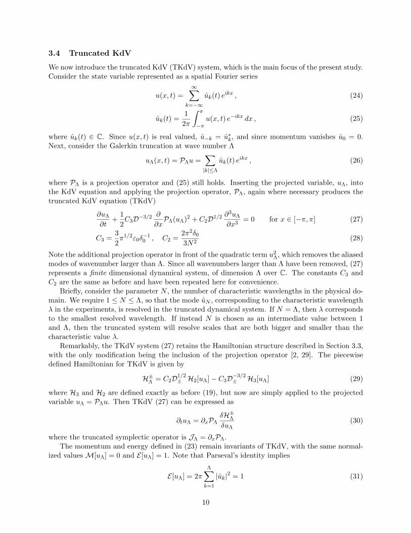
3.4 Truncated KdV

We now introduce the truncated KdV (TKdV) system, which is the main focus of the present study.Consider the state variable represented as a spatial Fourier series

u(x, t) =∞∑

k=−∞uk(t) e

ikx , (24)

uk(t) =1

2π

∫ π

−πu(x, t) e−ikx dx , (25)

where uk(t) ∈ C. Since u(x, t) is real valued, u−k = u∗k, and since momentum vanishes u0 = 0.Next, consider the Galerkin truncation at wave number Λ

uΛ(x, t) = PΛu =∑|k|≤Λ

uk(t) eikx , (26)

where PΛ is a projection operator and (25) still holds. Inserting the projected variable, uΛ, intothe KdV equation and applying the projection operator, PΛ, again where necessary produces thetruncated KdV equation (TKdV)

∂uΛ

∂t+

1

2C3D−3/2 ∂

∂xPΛ(uΛ)2 + C2D1/2 ∂

3uΛ

∂x3= 0 for x ∈ [−π, π] (27)

C3 =3

2π1/2ε0δ

−10 , C2 =

2π2δ0

3N2(28)

Note the additional projection operator in front of the quadratic term u2Λ, which removes the aliased

modes of wavenumber larger than Λ. Since all wavenumbers larger than Λ have been removed, (27)represents a finite dimensional dynamical system, of dimension Λ over C. The constants C3 andC2 are the same as before and have been repeated here for convenience.

Briefly, consider the parameter N , the number of characteristic wavelengths in the physical do-main. We require 1 ≤ N ≤ Λ, so that the mode uN , corresponding to the characteristic wavelengthλ in the experiments, is resolved in the truncated dynamical system. If N = Λ, then λ correspondsto the smallest resolved wavelength. If instead N is chosen as an intermediate value between 1and Λ, then the truncated system will resolve scales that are both bigger and smaller than thecharacteristic value λ.

Remarkably, the TKdV system (27) retains the Hamiltonian structure described in Section 3.3,with the only modification being the inclusion of the projection operator [2, 29]. The piecewisedefined Hamiltonian for TKdV is given by

H±Λ = C2D1/2± H2[uΛ]− C3D−3/2

± H3[uΛ] (29)

where H3 and H2 are defined exactly as before (19), but now are simply applied to the projectedvariable uΛ = PΛu. Then TKdV (27) can be expressed as

∂tuΛ = ∂xPΛδH±ΛδuΛ

(30)

where the truncated symplectic operator is JΛ = ∂xPΛ.The momentum and energy defined in (23) remain invariants of TKdV, with the same normal-

ized values M[uΛ] = 0 and E [uΛ] = 1. Note that Parseval’s identity implies

E [uΛ] = 2π

Λ∑k=1

|uk|2 = 1 (31)

10

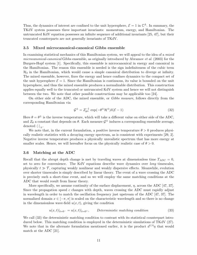
Thus, the dynamics of interest are confined to the unit hypersphere, E = 1 in CΛ. In summary, theTKdV system possesses three important invariants: momentum, energy, and Hamiltonian. Theuntruncated KdV equation possesses an infinite sequence of additional invariants [25, 47], but theirtruncated counterparts are not generally invariants of TKdV.

3.5 Mixed microcanonical-canonical Gibbs ensemble

In examining statistical mechanics of this Hamiltonian system, we will appeal to the idea of a mixedmicrocanonical-canonical Gibbs ensemble, as originally introduced by Abramov et al. (2003) for theBurgers-Hopf system [1]. Specifically, this ensemble is microcanonical in energy and canonical inthe Hamiltonian. The reason this ensemble is needed is the sign indefiniteness of the cubic termH3 in the Hamiltonian, which would cause a simple canonical distribution to diverge at infinity.The mixed ensemble, however, fixes the energy and hence confines dynamics to the compact set ofthe unit hypersphere E = 1. Since the Hamiltonian is continuous, its value is bounded on the unithypersphere, and thus the mixed ensemble produces a normalizable distribution. This constructionapplies equally well to the truncated or untruncated KdV system and hence we will not distinguishbetween the two. We note that other possible constructions may be applicable too [24].

On either side of the ADC, the mixed ensemble, or Gibbs measure, follows directly from thecorresponding Hamiltonian via

G± = Z−1θ± exp(−θ±H±)δ(E − 1) (32)

Here θ = θ± is the inverse temperature, which will take a different value on either side of the ADC,and Zθ a constant that depends on θ. Each measure G± induces a corresponding ensemble average,denoted 〈·〉±.

We note that, in the current formulation, a positive inverse temperature θ > 0 produces physi-cally realistic statistics with a decaying energy spectrum, as is consistent with experiments [29, 2].Negative inverse temperature produces a physically unrealistic spectrum that has more energy atsmaller scales. Hence, we will hereafter focus on the physically realistic case of θ > 0.

3.6 Matching at the ADC

Recall that the abrupt depth change is met by traveling waves at dimensionless time TADC = 0,set to zero for convenience. The KdV equations describe wave dynamics over long timescales,physically t� T , capturing weakly nonlinear and weakly dispersive effects. Meanwhile, evolutionover shorter timescales is simply described by linear theory. The event of a wave crossing the ADCis precisely such a short-time event, and so we will employ the same matching conditions at theADC that would result from linear theory.

More specifically, we assume continuity of the surface displacement, η, across the ADC [47, 37].Since the propagation speed c changes with depth, waves crossing the ADC must rapidly adjustin wavelength in order to match the oscillation frequency just upstream of the ADC [47, 37]. Thenormalized domain x ∈ [−π, π] is scaled on the characteristic wavelength and so there is no changein the dimensionless wave-field u(x, t), giving the condition

u(x, t)|t=0− = u(x, t)|t=0+ , Deterministic matching condition (33)

We call (33) the deterministic matching condition to contrast with its statistical counterpart intro-duced below. This matching condition is employed in the deterministic simulations of TKdV (27).We note that in the alternate formulation mentioned earlier, it is the product d1/4η that wouldmatch at the ADC [21].

11

Now, from the perspective of statistical mechanics, consider the communication between thestatistical ensembles, G±, upstream and downstream of the ADC. These two systems are in contactat the ADC, and so the upstream state with distribution G− can be regarded as a thermal reservoirthat influences the downstream distribution G+. In fact, the above deterministic condition directlyleads to a simple description for the link. The quantity of interest is the outgoing HamiltonianH+, since its value just upstream of the ADC, t = 0−, is set by the incoming dynamics, andthen this particular value is conserved thereafter in the outgoing dynamics. Since u matches atthe ADC, so must H+, and, in fact, this matching holds for every individual trajectory. Recallthat H+(t) is not conserved in the upstream dynamics and so its value varies for t < 0. However,appealing to weak Ergodicity, the ensemble mean 〈H+(t)〉− is expected to be independent of time.In particular, the value 〈H+|t=0−〉− is the same as the bare ensemble mean 〈H+〉−. Afterwards, theparticular value H+|t=0− is conserved in the downstream dynamics, on a trajectory-by-trajectorybasis and for all t > 0. Thus, the downstream measure G+ must recover the same ensemble mean〈H+|t=0−〉− = 〈H+〉−, producing the simple condition⟨

H+⟩− =

⟨H+⟩

+Statistical matching condition (34)

This statistical matching condition, originally derived by Majda et al. (2019) [29], imposes arelationship between the two inverse temperatures θ− and θ+. In particular, we view θ− as givenby the random-state of the incoming wave field. Thus, while we will treat θ− as a parameter thatcan be varied to study various possible system states, the downstream θ+ is determined directlyby the matching condition (34), giving the functional dependence

θ+ = F(θ−)

Transfer function (35)

The transfer function F will be a key link needed to relate the theory to experiments.

3.7 Numerical computation of the transfer function

To compute the transfer function, we use a weighted random-sampling strategy. That is, we firstsample the Fourier coefficients u = {uk}Λk=0 from a uniform distribution on the unit hypersphereE = 1. The uniform sampling is achieved by first sampling from an isotropic Gaussian distributionand then normalizing to project onto the hypersphere [1]. These samples are then weighted by theappropriate Gibbs measure (32) to compute the expectations needed in the statistical matchingcondition (34). That is, for an arbitrary quantity Q, the ensemble expectation corresponding toHamiltonian H and inverse temperature θ is numerically approximated as

〈Q〉θ =

∑Nsi=1Qi exp(−θHi)∑Nsi=1 exp(−θHi)

(36)

where Ns is the number of samples. Then, enforcing the statistical matching condition (34) becomesa root-finding problem for the function

W (θ+) =⟨H+⟩θ+−⟨H+⟩θ−

= 0 (37)

Recall that we consider θ− as given, so that 〈H+〉θ− is a constant that can be computed straightawayfrom (36). We then use the secant method with respect to the variable θ+ to find a root of W (θ+)to the desired tolerance.

For simply computing the transfer function, this weighted-sampling approach offers significantadvantages over more sophisticated methods, such as such Markov Chain Monte Carlo (MCMC),

12

in its ability to reuse the same samples of u for several different values of θ+. That is, we sample ufrom the uniform distribution and compute the list of Hamiltonian values only once, then simplyvary θ+ in (37) with the secant method until the root is found. An MCMC method, on the otherhand, would require the sampling to restart from scratch for each value of θ+, since the randomsteps in MCMC depend directly on the target distribution (32). We will however, use MCMC toinitialize direct numerical simulations of TKdV due to the superior efficiency for a single, givenvalue of θ.

3.8 Deterministic simulations of TKdV

We now detail the method for direct numerical simulation of the TKdV dynamical system (27). Inparticular, since the conservation of energy and Hamiltonian plays a central role in the emergentstatistical features of the system, it is important for the numerical scheme to conserve these quan-tities over long time horizons. We therefore employ a symplectic integrator, which, by preservingoriented areas in phase space, conserves the energy and Hamiltonian exactly.

Rearranging the TKdV system (27) gives

∂uΛ

∂t= −1

2C3D−3/2 ∂

∂xPΛ(uΛ)2 − C2D1/2 ∂

3uΛ

∂x3= F [uΛ] (38)

where we have represented the right-hand side by the operator F [uΛ]. We employ a pseudo-spectraldiscretization of (38), with de-aliasing applied to the quadratic nonlinear term PΛ(uΛ)2 accordingto the standard 2/3-rule. That is, we first pad uk with zeros for Λ < |k| ≤ 3Λ/2, transformto physical space and square to obtain u2

Λ on a fine grid, then transform back to spectral spaceand truncate to obtain the Fourier coefficients of PΛ(uΛ)2 For simplicity, we denote these Fouriercoefficients vk,

PΛ(uΛ)2 =∑|k|≤Λ

vkeikx (39)

With this discretization, (38) can be recast in spectral space as a nonlinear ODE system

d

dtuk = −1

2C3D−3/2 ikvk + C2D1/2 ik3uk = Fk (40)

The quadratic nonlinearity represented by vk mixes the modes during evolution. We note thethird-order linear term may become stiff for large Λ.

For time integration of (40), we employ a 4th-order midpoint symplectic scheme [31]. We

introduce the spectral vectors u = {uk}Λk=0 and F ={Fk

}Λ

k=0, and let un denote the solution at

time tn. The midpoint method has two intermediate stages and the auxiliary vectors y1,y2:

y1 − un = w1∆tF

[1

2(y1 + un)

], (41)

y2 − y1 = w2∆tF

[1

2(y2 + y1)

], (42)

un+1 − y2 = w3∆tF

[1

2

(un+1 + y2

)], (43)

with the time increments w1 =(2 + 21/3 + 2−1/3

)/3, w2 = 1−2w1, and w3 = w1. The semi-implicit

nature of (41)–(43) combined with the nonlinearity in F requires iteration. We split F into linearand nonlinear components, with the linear component being easily inverted since it is diagonal in

13

spectral space. At each step of (41)–(43), we perform Picard iteration on the nonlinear componentuntil convergence is achieved with a tolerance of δ = 1×10−10. The starting guess for the iterationsis determined by quadratic extrapolation from the previous three stages.

For the initial conditions, u0, of the direct numerical simulation we sample from the upstreamGibbs ensemble G− (32) with a prescribed inverse temperature θ−. We achieve this sampling via aMetropolis-Hasting Monte-Carlo algorithm as detailed in [29].

3.9 Scaling analysis to link inverse temperature to experiments

Since the inverse temperature, θ, is a key modeling parameter, it would be highly desirable tonormalize the system such that the value of θ does not depend sensitively on the truncation indexas Λ grows large. That way, θ can be interpreted as a real physical parameter that can be linkedto the experiments and whose value does not depend sensitively on where one chooses to truncatethe system. The one modeling parameter that is left to be set is N , which represents the numberof characteristic wavelengths in the periodic domain. In what follows, we will determine reasonableconstraints on N that allow θ to be asymptotically independent of Λ.

The invariant measure exhibits the proportionality GΛ ∝ exp(−θΛHΛ), where we have madeexplicit the dependence of all quantities on Λ. In particular, if HΛ were to depend sensitively on Λin expectation, then θΛ would need to compensate in order to produce the same invariant measure.Hence, it would be desirable to scale the system in such a way that HΛ does not depend sensitivelyon Λ, at least in expectation. To achieve this insensitivity, we will appeal to the uniform measure G0

and the idea of equipartition of energy [1], since these two concepts afford simple scaling estimates.Recall that HΛ is composed of the cubic and quadratic components H3 and H2. Due to the

odd symmetry of H3, it is easy to see that 〈H3〉0 = 0 with respect to the uniform measure G0. Thequadratic component, however, requires closer inspection. Due to Parseval’s identity, H2 can bewritten as

H2 =1

2

∫ π

−πu2x dx = 2π

Λ∑k=1

k2 |uk|2 (44)

Due to the constraint E [uΛ] = 1, the equipartioned microstate is given by

|uk|2 ≈1

2πΛfor equipartition of energy (45)

Then the expected value of H2 under the uniform measure is

〈H2〉0 = 2π

Λ∑k=1

k2⟨|uk|2

⟩0∼ 1

3Λ2 (46)

where we have used the identity for the Gauss-like sum

n∑k=1

k2 =1

6n(n+ 1)(2n+ 1) ≈ 1

3n3 (47)

Importantly, (46) shows that the expected value of H2 grows like Λ2, which appears problematicfor obtaining independence as Λ → ∞. However, H2 enters H in product with the coefficient C2,which itself scales as C2 ∼ N−2. Hence, obtaining the desired asymptotic independence with respectto Λ simply requires that N grow proportionally to Λ, as was already argued on physical groundsin Section 3.4. Thus, any of the choices N = Λ, Λ/2, or Λ/4, discussed in that section would be

14

Λ=12Λ=16Λ=20

0 5 10 15 20 250

5

10

15

20N = 8 fixed

incoming θ -

outg

oing

θ+

Λ=12Λ=16Λ=20

0 5 10 15 20 250

5

10

15

20N = Λ/2 scaled

incoming θ -

outg

oing

θ+

incomingoutgoing

0 5 10 15 20 250

0.2

0.4

0.6

0.8

1.0

Λ= 16, N = 8

incoming θ -

skew

(u)

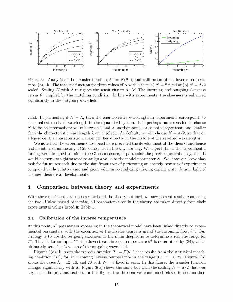
Figure 3: Analysis of the transfer function, θ+ = F (θ−), and calibration of the inverse tempera-ture. (a)–(b) The transfer function for three values of Λ with either (a) N = 8 fixed or (b) N = Λ/2scaled. Scaling N with Λ mitigates the sensitivity to Λ. (c) The incoming and outgoing skewnessversus θ− implied by the matching condition. In line with experiments, the skewness is enhancedsignificantly in the outgoing wave field.

valid. In particular, if N = Λ, then the characteristic wavelength in experiments corresponds tothe smallest resolved wavelength in the dynamical system. It is perhaps more sensible to chooseN to be an intermediate value between 1 and Λ, so that some scales both larger than and smallerthan the characteristic wavelength λ are resolved. As default, we will choose N = Λ/2, so that ona log-scale, the characteristic wavelength lies directly in the middle of the resolved wavelengths.

We note that the experiments discussed here preceded the development of the theory, and hencehad no intent of mimicking a Gibbs measure in the wave forcing. We expect that if the experimentalforcing were designed to mimic the Gibbs measure, in particular the precise spectral decay, then itwould be more straightforward to assign a value to the model parameter N . We, however, leave thattask for future research due to the significant cost of performing an entirely new set of experimentscompared to the relative ease and great value in re-analyzing existing experimental data in light ofthe new theoretical developments.

4 Comparison between theory and experiments

With the experimental setup described and the theory outlined, we now present results comparingthe two. Unless stated otherwise, all parameters used in the theory are taken directly from theirexperimental values listed in Table 1.

4.1 Calibration of the inverse temperature

At this point, all parameters appearing in the theoretical model have been linked directly to exper-imental parameters with the exception of the inverse temperature of the incoming flow, θ−. Ourstrategy is to use the outgoing skewness as the main diagnostic to determine a realistic range forθ−. That is, for an input θ−, the downstream inverse temperature θ+ is determined by (34), whichultimately sets the skewness of the outgoing wave-field.

Figures 3(a)-(b) show the transfer function θ+ = F(θ−) that results from the statistical match-ing condition (34), for an incoming inverse temperature in the range 0 ≤ θ− ≤ 25. Figure 3(a)shows the cases Λ = 12, 16, and 20 with N = 8 fixed in each. In this figure, the transfer functionchanges significantly with Λ. Figure 3(b) shows the same but with the scaling N = Λ/2 that wasargued in the previous section. In this figure, the three curves come much closer to one another.

15

-2.0 -1.5 -1.0 -0.5 0 0.5 1.0 1.5 2.00.01

0.1

1Upstream

upstream displacement, u-

p(u -)

-2.0 -1.5 -1.0 -0.5 0 0.5 1.0 1.5 2.00.01

0.1

1Downstream

downstream displacement, u+

p(u +)

-2.0 -1.5 -1.0 -0.5 0 0.5 1.0 1.5 2.00.01

0.1

1Upstream

upstream displacement, u-

p(u -)

-2.0 -1.5 -1.0 -0.5 0 0.5 1.0 1.5 2.00.01

0.1

1Downstream

downstream displacement, u+

p(u +)

Experiment histograms

TKdV histograms

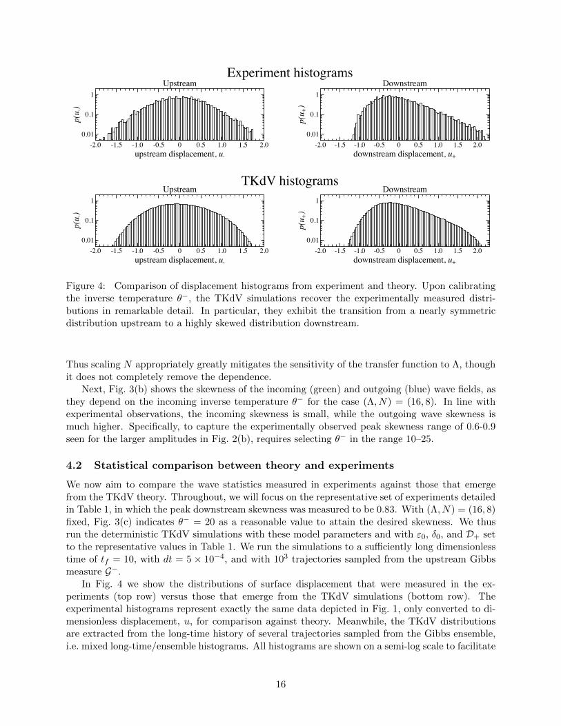
Figure 4: Comparison of displacement histograms from experiment and theory. Upon calibratingthe inverse temperature θ−, the TKdV simulations recover the experimentally measured distri-butions in remarkable detail. In particular, they exhibit the transition from a nearly symmetricdistribution upstream to a highly skewed distribution downstream.

Thus scaling N appropriately greatly mitigates the sensitivity of the transfer function to Λ, thoughit does not completely remove the dependence.

Next, Fig. 3(b) shows the skewness of the incoming (green) and outgoing (blue) wave fields, asthey depend on the incoming inverse temperature θ− for the case (Λ, N) = (16, 8). In line withexperimental observations, the incoming skewness is small, while the outgoing wave skewness ismuch higher. Specifically, to capture the experimentally observed peak skewness range of 0.6-0.9seen for the larger amplitudes in Fig. 2(b), requires selecting θ− in the range 10–25.

4.2 Statistical comparison between theory and experiments

We now aim to compare the wave statistics measured in experiments against those that emergefrom the TKdV theory. Throughout, we will focus on the representative set of experiments detailedin Table 1, in which the peak downstream skewness was measured to be 0.83. With (Λ, N) = (16, 8)fixed, Fig. 3(c) indicates θ− = 20 as a reasonable value to attain the desired skewness. We thusrun the deterministic TKdV simulations with these model parameters and with ε0, δ0, and D+ setto the representative values in Table 1. We run the simulations to a sufficiently long dimensionlesstime of tf = 10, with dt = 5 × 10−4, and with 103 trajectories sampled from the upstream Gibbsmeasure G−.

In Fig. 4 we show the distributions of surface displacement that were measured in the ex-periments (top row) versus those that emerge from the TKdV simulations (bottom row). Theexperimental histograms represent exactly the same data depicted in Fig. 1, only converted to di-mensionless displacement, u, for comparison against theory. Meanwhile, the TKdV distributionsare extracted from the long-time history of several trajectories sampled from the Gibbs ensemble,i.e. mixed long-time/ensemble histograms. All histograms are shown on a semi-log scale to facilitate

16

-1.0 -0.5 0 0.5 1.00.01

0.1

1

Upstream

surface slope, ηx

p(η x)

-1.0 -0.5 0 0.5 1.00.01

0.1

1

Downstream

surface slope, ηx

p(η x)

-1.0 -0.5 0 0.5 1.00.01

0.1

1

Upstream

surface slope, ηx

p(η x)

-1.0 -0.5 0 0.5 1.00.01

0.1

1

Downstream

surface slope, ηx

p(η x)

Experiment histograms

TKdV histograms

Figure 5: Comparison of surface slope histograms. The experiments and TKdV simulations showvery similar slope distributions upstream. Downstream, the theory accounts for the spread of thedistribution and the long exponential tails, while differences in the detailed shape of the distribu-tions are also visible. Note the elevated uncertainty in the experimental data due to numericaldifferentiation of free-surface measurements.

comparison of the tails, where extreme events lie.The comparison between experiments and theory in Fig. 4 is striking. As seen in the figure, both

the experiments and theory show a transition from a nearly symmetric upstream distribution to ahighly skewed distribution downstream. The TKdV theory not only captures this transition, butalso recovers the shape of the resulting downstream distribution in remarkable detail. Nearly everyfeature that can be compared — the decay rate of the tail, the position and value of the peak, therapid cutoff for negative u — matches surprisingly well. This comparison offers compelling visualevidence for: (a) the predictive power of the TKdV framework, and (b) the successful calibrationof the incoming inverse temperature.

Next, we aim to make the same comparison for free-surface slopes. We note that the derivative,∂η/∂x, is already a dimensionless quantity with a simple physical interpretation, namely the slopeof the free surface, whereas the interpretation of ∂u/∂x is tied to the characteristic values A andL. We therefore convert the theoretical calculated slopes values back to physical slopes via

∂η

∂x= 2π3/2 ηstd

λ±

∂u±∂x

(48)

So that the peak experimental wavelength λ (corresponding to fp = 2 Hz) would be mapped to thedominating TKdV spectral mode, k = 1, this conversion formula has not been corrected with theextra factor of N present in (12).

Figure 5 shows the distributions of surface slope that result from experiments (top) and theory(bottom). These histograms show intriguing similarities and differences. First, the upstream slopedistribution is captured well by the TKdV simulations, both in its nearly symmetric shape and itsscale. We note that, while the standard deviation of displacement was input into the TKdV theory,

17

the slope standard deviation was not. Downstream, both the experimental and theoretical slopedistributions spread significantly. Interestingly, in the experiments, it is not the standard deviationthat increases significantly upon crossing the depth change (std(ηx) increases from 0.15 to 0.17),but instead the excess kurtosis, which jumps from a value of 0.46 upstream to 3.4 downstream.Likewise, in the TKdV theory, std(ηx) grows from 0.13 upstream to 0.33 downstream, and kurt(ηx)grows from -0.04 to 0.50. Thus, the theoretically predicted jump in kurtosis, though not as extremeas that measured in experiments, is quite significant. These elevated levels of kurtosis are associatedwith the distinct appearance of the downstream distributions, most notably the long, flat tails thatappear in both experiments and theory.

Differences in the detailed shapes of these downstream distributions are also visible. First, wepoint out that the experimental measurements involve numerical differentiation of surface displace-ment extracted from optical images, a process that unavoidably amplifies any noise that is present.We must therefore proceed with caution in comparing the experiment and theory, recognizing thepossibility that observed discrepancies may be due to these measurement errors. Nonetheless, wenotice that the theoretically predicted distributions remain symmetric downstream and the ex-perimental ones skew towards negative slope. As mentioned in Section 2, negative skewness isconsistent with a right-moving wave of steep leading surface (i.e. negative slope). Additionally, thepeak of the experimental distribution appears sharper than that of the theory.

4.3 Wave dynamics and analysis of time scales

As a complement to the above statistical comparison, we now examine the wave dynamics of afew individual trajectories from the TKdV simulations. Figure 6 shows example upstream anddownstream solution trajectories from the same TKdV simulations that were used to produce thehistograms in Figs. 4–5. The dimensionless displacement, u, is represented by color in the domain(x, t) ∈ [−π, π]× [−10, 10], where the ADC is encountered at t = 0.

Visual differences between the upstream and downstream dynamics are apparent in Fig. 6. Theupstream trajectory shows several waves of modest amplitude all propagating leftward. Here, themagnitude of the positive and negative displacements are comparable. This is in stark contrastto the downstream dynamics, which feature fewer waves of larger amplitude propagating in eitherdirection. In particular, one large wave is seen to propagate from the lower-left corner of the figureto the upper right. A bias towards positive surface displacement is apparent in these downstreamdynamics, without even viewing the histograms.

These observations can be rationalized with some simple observations regarding the structureof the TKdV system. Upstream of the ADC, since D = 1, the nonlinear effects are relativelyweak and the dynamics are dominated by dispersion. Linearizing (27) and introducing the ansatzuk = ei(kx−ωkt) produces the dispersion relation for angular frequency ωk = −C2k

3, or for phasevelocity ck = ωk/k = −C2k

2 [30]. In particular, the phase velocity is strictly negative, implyingthat waves only propagate leftwards, as is consistent with Fig. 6(a).

Downstream of the ADC, however, the depth ratio changes to D = 0.24. This change signifi-cantly amplifies nonlinearity while suppressing dispersion, and thereby allows waves to propagatein either direction. In particular, the dispersionless limit of KdV is the Burgers-Hopf equation, forwhich the nonlinear advection is proportional in both amplitude and direction to the value of u.Hence, positive displacements would be expected to move rightwards, as is seen in Fig. 6(b).

We remind the reader that the KdV framework tracks the long-time evolution of waves in areference frame moving with the characteristic speed c =

√gd from linear theory. Hence, the above

discussion of left-or-right going waves cannot be interpreted in the context of the experimentswithout an appropriate Galilean transformation. Thus, in the laboratory frame, all waves indeed

18

-2

-1.5

-1

-0.5

0

0.5

1

1.5

2Upstream

-2 0 2-10

-9

-8

-7

-6

-5

-4

-3

-2

-1

0

normalized space

norm

aliz

ed ti

me

-2

-1.5

-1

-0.5

0

0.5

1

1.5

2Downstream

-2 0 20

1

2

3

4

5

6

7

8

9

10

normalized space

norm

aliz

ed ti

me

Figure 6: Sample upstream and downstream solution trajectories from the same ensemble TKdVsimulations featured in Figs. 4 and 5. The upstream solutions exhibit only leftward propagat-ing waves and a high degree of regularity, while the downstream solutions exhibit both left andrightward moving waves along with more intermittency.

propagate unidirectionally, from left to right, with a speed near c. The directions and speedscalculated by the TKdV framework simply quantify the deviation of the true wave speed from c.

Finally, Fig. 6 sheds some light on the timescales required for wave evolution in the TKdVframework. It appears that the normalized time of t = 10 is roughly the correct timescale toobserve substantial wave dynamics. More precisely, both the left-going waves in Fig. 6(a) and theright-going waves in Fig. 6(b) require a dimensionless time of about t = 7 to traverse the entireperiodic domain. For the representative experiments, the characteristic timescale, T , is 2.8 secupstream and 5.7 sec downstream. Hence, a dimensionless time of t = 7 corresponds to roughly20 sec and 40 sec upstream and downstream respectively. Given the wave speeds (c = 110 cm/supstream and 54 cm/s downstream), these timescales can be converted to distances traveled by thewaves. In fact, a simple calculation using the definitions in Section 3 gives the distance traveledas 7Ng/(2πf2

p ), which, due to a serendipitous cancellation, is independent of depth. Hence, thedistance traveled by the waves over a dimensionless time of t = 7 is the same value upstream anddownstream, roughly 22 meters. Note that this distance is significantly greater than the 6-meterlength of the experimental wave tank.

These estimates raise an important question: if a distance of 22 meters is required for significantwave evolution under the KdV framework, how do the experiments exhibit substantial changes inwave statistics a much shorter distance downstream of the ADC? The results shown in Fig. 7 helpresolve this question. This figure shows the evolution of surface-displacement skewness (left) andkurtosis (right) computed by the same deterministic TKdV simulations as pictured in Fig. 6. Thebold black curve shows the ensemble mean (ensemble size of 1000), while the faint gray curves showthe skewness and kurtosis of 100 individual trajectories to give a sense for the variation involved.Importantly, the skewness and kurtosis evolve on a much shorter timescale than the aforementioned

19

-10 -5 0 5 10

0

1

normalized time

skew

(u)

-10 -5 0 5 10-1

0

1

normalized time

kurt(u)

Figure 7: Dynamic evolution of surface-displacement skewness and kurtosis from the TKdVsimulations. Faint gray curves show skewness and kurtosis of 100 individual trajectories, and thebold black curves show the corresponding ensemble mean. Skewness and kurtosis evolve over muchshorter timescales than that required for waves to cross the domain.

t = 7. More precisely, skewness and kurtosis have already saturated to their asymptotic value byt = 1, and reach half of that value by t = 0.18. These dimensionless times correspond to traveldistances of 310 cm and 56 cm respectively — much shorter than the previously mentioned 22meters, and on the same order as the relevant distances in the experiments. Thus, after crossingthe ADC, the wave-field rapidly reconfigures itself enough to fundamentally alter its statisticaldistributions, and the timescale for this reconfiguration is much shorter than the time required forwaves to cross the entire periodic domain.

4.4 Explicit formula for outgoing skewness and experimental confirmation

We now discuss arguably the most novel single result of the manuscript. In the recent theoreticalstudy, Majda et al. (2019) derived an explicit formula for the outgoing wave-field skewness in termsof the system parameters [29]. More specifically, this formula relates the downstream skewness ofsurface displacement, skew(η), to the change in slope variance, var(ηx). Here, we recap the deriva-tion of this formula and then test the prediction against new, direct experimental measurements.

The explicit formula for outgoing skewness arises directly from the statistical matching condition(34), which states that the downstream Hamiltonian must match in expected value at the ADC,i.e. with respect to the incoming and outgoing Gibbs measures. This condition can be written moreexplicitly as

C2D1/2+ 〈H2〉− − C3D−3/2

+ 〈H3〉− = C2D1/2+ 〈H2〉+ − C3D−3/2

+ 〈H3〉+ (49)

Both the experiments and simulations show the upstream skewness to be negligible compared toits downstream counterpart, allowing the term with 〈H3〉− to be dropped in (49). With thisapproximation, (49) yields the relationship

〈H3〉+〈H2〉+ − 〈H2〉−

=C2

C3D2

+ (50)

Our next task is to convert this formula to physical variables so that it can be tested againstexperimental data. First, following the definition of H3 in (19) and the definition, u = η/(π1/2ηstd),a straightforward calculation gives

〈H3〉+ =π

3

⟨u3⟩

+=

1

3π1/2

⟨η3⟩

+

η3std

=1

3π1/2skew+(η) (51)

20

slope = -3

0.005 0.01 0.02

102

103

104

wave amplitude, ε0

skew

(η) /

Δva

r(η x

)

-10 0 10 20 30 40 50

0

0.5

1.0sk

ew(η

)

-10 0 10 20 30 40 500

0.01

0.02

0.03

0.04

position, x (cm)

var(η x

)(a)

(b)

(c)

Figure 8: Experimental confirmation of the explicit formula for outgoing skewness (53). (a)–(b)Spatial variation of skew(η) and var(ηx) for several different amplitudes. The maximum of skew(η)and the minimum of var(ηx) each occur at a location that is insensitive to amplitude, x =15 cm(blue) and -9 cm (green) respectively. (c) Measurements of the ratio skew(η)/∆var(ηx) from 15different experiments plotted against the dimensionless wave amplitude ε0. For sufficiently largeamplitude, the measurements follow the predicted ε−3

0 power law closely.

This equation expresses a direct relationship between the expected value of H3 and the outgoingskewness of surface displacement. Next, we must convert the H2-quantities, which involve surfaceslope. Using the definition of H2 in (19) and L+ in (12) gives

〈H2〉± = π⟨u2x

⟩± =

(Nλ+

2πηstd

)2

var±(ηx) (52)

We note that the downstream scale L+ is used in this conversion, since it is the downstreamHamiltonian that is matched in (34). This formula links the expected value of H2 to the varianceof surface slope.

Inserting (51) and (52) into (50), and using the definitions of C2 and C3 from (14), gives theremarkably explicit formula

skew+(η)

var+(ηx)− var−(ηx)=

1

3ε−3

0 D3+ (53)

This formula links the skewness of the outgoing wave field to the change in the variance of surfaceslope. In particular, it predicts their ratio to scale as the inverse cube of wave amplitude, ε−3

0 ,and the cube of the depth ratio, D3

+. It is a rather unexpected relationship, as it would have beendifficult to anticipate that the displacement skewness and slope variance, among all possible variablecombinations, are so intimately related.

Fortunately, it is a relationship that can be tested directly against the experimental measure-ments, specifically the type of data that was presented in Fig. 2. Formula (53) draws focus tothe spatial variation of displacement skewness, which we replot for convenience in Fig. 8(a), andthe variance of surface slope, shown in Fig. 8(b). To test (53), we must select a representativedownstream position to evaluate skew+(η) and var+(ηx), and a representative upstream positionfor var−(ηx). In short, we select the same representative locations used to evaluate the histogramsin Figs. 1, 4, and 5, namely x = 15 cm downstream and x = −9 cm upstream. These positionsare indicated by the blue and green vertical dashed lines in Fig. 8(a)–(b). Recall that x = 15 cm

21

corresponds to the peak of the downstream skewness and kurtosis. Meanwhile, we see in Fig. 8(b)that x = −9 cm corresponds to a slight dip in var(ηx).

With these locations selected, we evaluate the ratio skew(η)/∆var(ηx) for each experiment andplot the result against dimensionless wave amplitude, ε0 = ηstd/d− on a log-log scale in Fig. 8(c).While the data shows significant variation at small amplitudes, it shows a well defined decreasingtrend at larger amplitudes. In particular, the red dashed line shows the power-law ε−3

0 predictedby (53), which captures the experimental trend remarkably well.

5 Concluding remarks

This manuscript extends the parallel experimental and modeling efforts of Bolles et al. (2019) [5]and Majda et al. (2019) [29] concerning the emergence of anomalous wave statistics from abruptchanges in bottom topography. The theoretical framework is based on deterministic and statisticalanalysis of the TKdV system, with exploitation of the Hamiltonian structure and the associatedinvariant Gibbs measures. The theory depends crucially on matching the incoming and outgoinginvariant measures at the abrupt depth change, so as to link the incoming and outgoing states.Throughout, we have emphasized the synergy between the experiments and theory, with experimen-tal data informing theoretical advancements and model predictions motivating new experimentalmeasurements.

Careful calibration of the inverse temperature against the experimental data allowed for adetailed comparison between experimental and theoretically predicted wave statistics. The outgoingdistributions of surface displacement predicted by the TKdV framework capture in remarkabledetail the experimental measurements. We have extended this statistical analysis to surface slope,a line of inquiry motivated by the importance ofH2, the slope standard deviation, in the theory. Thecomparison of slope statistics shows intriguing similarities, while also some quantitative differencesin the shape and skewness of the outgoing distributions.

Finally, Majda et al. (2019) [29] derived an explicit formula for the skewness of the outgoingwave field, which we have tested against direct experimental measurements. Specifically, the for-mula predicts how the ratio of displacement skewness to slope variance, skew(η)/∆var(ηx), dependson wave amplitude. The experimental measurements conclusively confirm the inverse-cube depen-dence on wave amplitude, thus highlighting the predictive power of the TKdV statistical mechanicsframework.

We note that since the ratio, skew(η)/∆var(ηx), exhibits such a clear dependence on inputparameters, it could prove a useful diagnostic for anomalous wave observations in the ocean. Inparticular, this quantity seems to provide a signature for anomalous waves that are triggered byabrupt depth changes. Examination of this ratio in field data is an exciting avenue for futureresearch.

Acknowledgements

CTB acknowledges support from the IDEA grant at Florida State University, as well as from theGeophysical Fluid Dynamics Institute. MNJM acknowledges support from the Simons Foundation,award 524259. This research of A.J.M. is partially supported by the Office of Naval ResearchN00014-19-S-B001. D.Q. is supported as a postdoctoral fellow on the grant.

22

References

[1] Rafail V Abramov, Gregor Kovacic, and Andrew J Majda. Hamiltonian structure and statisti-cally relevant conserved quantities for the truncated Burgers-Hopf equation. Communicationson Pure and Applied Mathematics: A Journal Issued by the Courant Institute of MathematicalSciences, 56(1):1–46, 2003.

[2] J Bajars, JE Frank, and BJ Leimkuhler. Weakly coupled heat bath models for Gibbs-likeinvariant states in nonlinear wave equations. Nonlinearity, 26(7):1945, 2013.

[3] T Brooke Benjamin and JE Feir. The disintegration of wave trains on deep water part 1.theory. Journal of Fluid Mechanics, 27(03):417–430, 1967.

[4] Patrick J Blonigan, Mohammad Farazmand, and Themistoklis P Sapsis. Are extreme dissipa-tion events predictable in turbulent fluid flows? Physical Review Fluids, 4(4):044606, 2019.

[5] C Tyler Bolles, Kevin Speer, and MNJ Moore. Anomalous wave statistics induced by abruptdepth change. Physical Review Fluids, 4(1):011801, 2019.

[6] Roberto Camassa, Richard M McLaughlin, Matthew NJ Moore, and Kuai Yu. Stratified flowswith vertical layering of density: experimental and theoretical study of flow configurations andtheir stability. Journal of Fluid Mechanics, 690:571–606, 2012.

[7] Jinbing Chen and Dmitry E Pelinovsky. Periodic travelling waves of the modified KdV equationand rogue waves on the periodic background. Journal of Nonlinear Science, 29(6):2797–2843,2019.

[8] Nan Chen and Andrew J Majda. Filtering nonlinear turbulent dynamical systems throughconditional Gaussian statistics. Monthly Weather Review, 144(12):4885–4917, 2016.

[9] Peter A Clarkson and Ellen Dowie. Rational solutions of the Boussinesq equation and ap-plications to rogue waves. Transactions of Mathematics and its Applications, 1(1):tnx003,2017.

[10] Will Cousins and Themistoklis P Sapsis. Unsteady evolution of localized unidirectional deep-water wave groups. Physical Review E, 91(6):063204, 2015.

[11] Giovanni Dematteis, Tobias Grafke, Miguel Onorato, and Eric Vanden-Eijnden. Experimentalevidence of hydrodynamic instantons: The universal route to rogue waves. arXiv preprintarXiv:1907.01320, 2019.

[12] Giovanni Dematteis, Tobias Grafke, and Eric Vanden-Eijnden. Rogue waves and large devia-tions in deep sea. Proceedings of the National Academy of Sciences, 115(5):855–860, 2018.

[13] Mohammad Farazmand and Themistoklis P Sapsis. Reduced-order prediction of rogue wavesin two-dimensional deep-water waves. Journal of Computational Physics, 340:418–434, 2017.

[14] Likhit Ganedi, Anand U Oza, Michael Shelley, and Leif Ristroph. Equilibrium shapes andtheir stability for liquid films in fast flows. Physical Review Letters, 121(9):094501, 2018.

[15] Chris Garrett and Johannes Gemmrich. Rogue waves. Phys. Today, 62(6):62, 2009.

23

[16] O Gramstad, H Zeng, K Trulsen, and GK Pedersen. Freak waves in weakly nonlinear unidi-rectional wave trains over a sloping bottom in shallow water. Physics of Fluids, 25(12):122103,2013.

[17] Stephen Guth and Themistoklis P Sapsis. Machine learning predictors of extreme eventsoccurring in complex dynamical systems. Entropy, 21(10):925, 2019.

[18] EJ Heller, L Kaplan, and A Dahlen. Refraction of a Gaussian seaway. Journal of GeophysicalResearch: Oceans, 113(C9), 2008.

[19] James G Herterich and Frederic Dias. Extreme long waves over a varying bathymetry. Journalof Fluid Mechanics, 878:481–501, 2019.

[20] Darryl D Holm. A stochastic closure for wave–current interaction dynamics. Journal ofNonlinear Science, 29(6):29873031, 2019.

[21] Robin Stanley Johnson. A modern introduction to the mathematical theory of water waves,volume 19. Cambridge university press, 1997.

[22] I Karmpadakis, C Swan, and M Christou. Laboratory investigation of crest height statisticsin intermediate water depths. Proceedings of the Royal Society A, 475(2229):20190183, 2019.

[23] Christian Kharif, J-P Giovanangeli, Julien Touboul, Laurent Grare, and Efim Pelinovsky.Influence of wind on extreme wave events: experimental and numerical approaches. Journalof Fluid Mechanics, 594:209–247, 2008.

[24] Richard Kleeman and Bruce E Turkington. A nonequilibrium statistical model of spec-trally truncated Burgers-Hopf dynamics. Communications on Pure and Applied Mathematics,67(12):1905–1946, 2014.

[25] Peter D Lax. Periodic solutions of the KdV equation. Communications on Pure and AppliedMathematics, 28(1):141–188, 1975.

[26] AMS Macedo, Ivan R Roa Gonzalez, DSP Salazar, and GL Vasconcelos. Universality classes offluctuation dynamics in hierarchical complex systems. Physical Review E, 95(3):032315, 2017.

[27] A. Majda and D. Qi. Strategies for reduced-order models for predicting the statistical re-sponses and uncertainty quantification in complex turbulent dynamical systems. SIAM Review,60(3):491–549, 2018.

[28] Andrew J Majda. Introduction to turbulent dynamical systems in complex systems. Springer,2016.

[29] Andrew J Majda, MNJ Moore, and Di Qi. Statistical dynamical model to predict extremeevents and anomalous features in shallow water waves with abrupt depth change. Proceedingsof the National Academy of Sciences, 116(10):3982–3987, 2019.

[30] Andrew J Majda and Di Qi. Statistical phase transitions and extreme events in shallow waterwaves with an abrupt depth change. Journal of Statistical Physics, pages 1–24, 2019.

[31] Robert McLachlan. Symplectic integration of hamiltonian wave equations. Numerische Math-ematik, 66(1):465–492, 1993.

[32] Peter Muller, Chris Garrett, and A Osborne. Rogue waves. Oceanography, 18(3):66, 2005.

24

[33] Miguel Onorato, Davide Proment, and Alessandro Toffoli. Triggering rogue waves in opposingcurrents. Physical Review Letters, 107(18):184502, 2011.

[34] Efim Pelinovsky, Tatiana Talipova, and Christian Kharif. Nonlinear-dispersive mechanism ofthe freak wave formation in shallow water. Physica D: Nonlinear Phenomena, 147(1-2):83–94,2000.

[35] D Howell Peregrine. Water waves, nonlinear Schrodinger equations and their solutions. TheANZIAM Journal, 25(1):16–43, 1983.

[36] Di Qi and Andrew J. Majda. Using machine learning to predict extreme events in complexsystems. Proceedings of the National Academy of Sciences, 2019.

[37] Vincent Rey, Max Belzons, and Elisabeth Guazzelli. Propagation of surface gravity waves overa rectangular submerged bar. Journal of Fluid Mechanics, 235:453–479, 1992.

[38] Leif Ristroph, Matthew N. J. Moore, Stephen Childress, Michael J. Shelley, and Jun Zhang.Sculpting of an erodible body in flowing water. Proceedings of the National Academy of Sci-ences, 109(48):19606–19609, 2012.

[39] Themistoklis P Sapsis and Andrew J Majda. Blending modified Gaussian closure and non-Gaussian reduced subspace methods for turbulent dynamical systems. Journal of NonlinearScience, 23(6):1039–1071, 2013.

[40] Themistoklis P Sapsis and Andrew J Majda. Statistically accurate low-order models for un-certainty quantification in turbulent dynamical systems. Proceedings of the National Academyof Sciences, 110(34):13705–13710, 2013.

[41] Themistoklis P Sapsis and Andrew J Majda. A statistically accurate modified quasilinearGaussian closure for uncertainty quantification in turbulent dynamical systems. Physica D:Nonlinear Phenomena, 252:34–45, 2013.

[42] A Toffoli, D Proment, H Salman, J Monbaliu, F Frascoli, M Dafilis, E Stramignoni, R Forza,M Manfrin, and Miguel Onorato. Wind generated rogue waves in an annular wave flume.Physical Review Letters, 118(14):144503, 2017.

[43] Karsten Trulsen, Anne Raustøl, Stian Jorde, and Lisa Bæverfjord Rye. Extreme wave statisticsof long-crested irregular waves over a shoal. Journal of Fluid Mechanics, 882, 2020.

[44] Claudio Viotti and Frederic Dias. Extreme waves induced by strong depth transitions: Fullynonlinear results. Physics of Fluids, 26(5):051705, 2014.

[45] Claudio Viotti, Denys Dutykh, John M Dudley, and Frederic Dias. Emergence of coherentwave groups in deep-water random sea. Physical Review E, 87(6):063001, 2013.

[46] Benjamin S White and Bengt Fornberg. On the chance of freak waves at sea. Journal of FluidMechanics, 355:113–138, 1998.

[47] Gerald Beresford Whitham. Linear and nonlinear waves, volume 42. John Wiley & Sons,2011.

[48] LH Ying, Z Zhuang, EJ Heller, and L Kaplan. Linear and nonlinear rogue wave statistics inthe presence of random currents. Nonlinearity, 24(11):R67, 2011.

25