Sensors 2008, 8, 897-909

sensors ISSN 1424-8220 © 2008 by MDPI

www.mdpi.org/sensors

Full Paper

Networked Estimation with an Area-Triggered Transmission Method

Vinh Hao Nguyen and Young Soo Suh * Department of Electrical Engineering, University of Ulsan, Namgu, Ulsan 680-749, Korea E-mail: vinhhao@hcmut.edu.vn. E-mail: suh@ieee.org * Author to whom correspondence should be addressed. Email: suh@ieee.org

Received:18 January 2008 / Accepted: 7 February 2008 / Published: 15 February 2008

Abstract: This paper is concerned with the networked estimation problem in which sensor data are transmitted over the network. In the event-driven sampling scheme known as level-crossing or send-on-delta, sensor data are transmitted to the estimator node if the difference between the current sensor value and the last transmitted one is greater than a given threshold. The event-driven sampling generally requires less transmission than the time-driven one. However, the transmission rate of the send-on-delta method becomes large when the sensor noise is large since sensor data variation becomes large due to the sensor noise. Motivated by this issue, we propose another event-driven sampling method called area-triggered in which sensor data are sent only when the integral of differences between the current sensor value and the last transmitted one is greater than a given threshold. Through theoretical analysis and simulation results, we show that in the certain cases the proposed method not only reduces data transmission rate but also improves estimation performance in comparison with the conventional event-driven method.

Keywords: Networked estimation, event-driven, level-crossing, send-on-delta.

1. Introduction

The traditional way to transmit sensor data in networked control systems is to sample sensor signals equidistant in time. This approach is widely used since analysis and design are simple and inherited from well-established control system theories. If the network speed is high and the traffic is sparse, the periodic sampling approach has many merits because network-induced delay is small and can be

Sensors 2008, 8

898

ignored. But when the network bandwidth is limited due to executing tasks of several nodes, time delay becomes large and randomly varying. To avoid these problems, the sensor data transmission rate should be reduced.

Recent works have discussed event-driven alternatives to traditional time-triggered sampling scheme. It has been shown to be more efficient than time-triggered one in some situations, especially in network bandwidth improvement. For instance in [1], the authors provided a comparison of time-triggered impulse control and level-triggered one where the level-triggered scheme gave lower average error for the same average rate of impulse. In [2, 3], an adjustable deadband was defined on each node to reduce network traffic. The node does not broadcast a new message if its signal is within the deadband. A level-crossing sampling scheme in association with an 1-bit coding and decoding strategy to reduce data size was introduced in [4]. This coding sampling scheme becomes highly efficient under data-rate constraints since the nodes only transmit one bit, 0 or 1, per sample. In [5], an optimal level-triggered sampling design problem was proposed in order to minimize the distortion of a filter over a finite horizon. A similar sampling scheme named send-on-delta (SOD) transmission was explored in [6-8]. By adjusting the threshold value at each sensor node, data transmission rate is reduced in order for the network bandwidth to increase and can be used for other traffic. Although the event-driven schemes mentioned above have several names, the basic principle of sampling is the same. That is, in framework of networked control system, a sensor node transmits data only if the difference Δ between the current sensor value and the last transmitted one is greater than a given threshold. Hereafter, for ease in representation we refer to them as SOD sampling.

One major issue of SOD sampling method as pointed out in [9] is that it does not detect signal oscillations or steady-state error if the difference Δ remains within the threshold range during a long time. Furthermore, in highly noisy systems, the sensor value could exceed the threshold not because the true value exceeds the threshold but because sensor noise exceeds the threshold. In that case, there could be many unnecessary sensor data transmissions.

Motivated by the perspective results of the event-based integral sampling in [9] and the networked estimation problem using SOD transmission method in [7], we propose a novel sampling scheme called area-triggered or send-on-area (SOA) in which sensor data are sent only when the integral of Δ is greater than a given threshold. The proposed SOA sampling scheme is slightly different from [9] to improve bandwidth network in case of large noise. Then, a networked estimator based on Kalman filter is formulated to estimate states of the system periodically even when the sensor nodes do not transmit data. Through theoretical analysis and simulation results, we show that in the certain cases the proposed method gives better estimation performance than the SOD method in [7].

2. Area-triggered sampling scheme

Consider a networked control system described by the linear continuous-time model:

( ) ( ) ( ) ( )

( ) ( ) ( )

x t Ax t Bu t w t

y t Cx t v t

= + +

= + (1)

where is the state of the plant, u is the deterministic input signal, is the measurement output which is sent to the estimator node by the sensor nodes. is the process noise with

nx R∈ py R∈( )w t

Sensors 8

,i

, ,( , ) ( ( ) ) i last i i last it t y t yΠ ∫

2008,

lasty

( )v t

( ≤ ≤

899

( )v tcovariance Q , and is the measurement noise with covariance R . We assume that and are uncorrelated, zero mean white Gaussian random processes.

( )w t

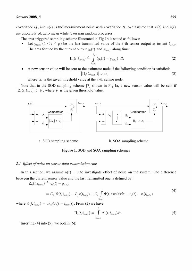
The area-triggered sampling scheme illustrated in Fig.1b is stated as follows: • Let ) be the last transmitted value of the i -th sensor output at instant ,last it .

The area formed by the current output ( )iy t and ,last iy along time: 1 i p

.dt−t

(2) ,last it

• A new sensor value will be sent to the estimator node if the following condition is satisfied: ,( , )i last i it t αΠ > (3)

where is the given threshold value at the i -th sensor node. iα

Note that in the SOD sampling scheme [7] shown in Fig.1a, a new sensor value will be sent if ,( ,i last it t δΔ > iδ

( ) 0=

, ,( , ) ( )i last i last it t t yΔ −

,

)i , where is the given threshold value.

a. SOD sampling scheme b. SOA sampling scheme

Figure 1. SOD and SOA sampling schemes

2.1. Effect of noise on sensor data transmission rate

In this section, we assume u t to investigate effect of noise on the system. The difference between the current sensor value and the last transmitted one is defined by:

[ ],

, ,( , ) ( ) ( , ) ( ) ( ) ( )last i

t

last i last i i i i last i

t

C t t I x t C t r w r v t v t= Φ − + Φ + −∫

,( , ) ( ))last i last it t A t tΦ = −t

,

i

i

y

, exp(

r d

.

(4)

where . From (2) we have:

,

,( , ) ( , )last i

i last i i last i

t

t t t t drΠ = Δ∫ (5)

Inserting (4) into (5), we obtain (6):

( )iy t ,last iy

iΔ

iδ

+_

sTComparator

i iδΔ >

( )iy t ,st i

iΔ

lay

∫ iΠ

iα

sT

+_

Comparator

i iαΠ >

Sensors 2008,

900

( , )

st i

iC u r du+ Φ⎢∫,

,( ) ( ) .t

i i last i

t

w r dr v t dr+ −⎥ ∫

,

,

,( , ( 2 ( , )last i

t

last i

t

i dr

C t r Q C R i i t tθ θ= + −∫( , )R i i )i i

( ), ( , ) .t r u r duθ Φ∫

{ } ) 2 ( , )i iE C t r C R i i′Δ Δ = Φ

}

iα

8

[ ]

[ ]

[ ]

,

,

, , ,

,

, ,

, ,

,

, ,

( , ) ( , )

( , ) ( )

( , ) ( ) ( ) ( )

( , ) ( )

last i

last i

last i last i last i

last i

t

i last i i last i

t

t

i last i last i

t

t u t

i i i la

t t t

t

i last i last i

t

t

t t t t dr

C t t I x t dr

C t r w r drdu v t v t dr

C t t I x t dr

Π = Δ

= Φ −

+ Φ + −

= Φ −

⎡ ⎤⎢ ⎥

∫

∫

∫ ∫ ∫

∫t t

(6)

r⎢⎣ ⎦, ,last i last i last i⎥

,( ) 0last ix t = ,( , )i last it tΠ

( )

,

{ } ( , ) ( ) ( ) ( , ) 2 ( , )last i last i

t t

i i i i

t

t

E C t r w r w r t r drC R iθ θ′ ′′ ′Π Π = +

′′

∫ ∫

( )t t

v t dr∫ ∫Assuming , we can derive the variance of as follows

(7)

) , )i it r dr

where is the ( , -th element of R and is defined by ( ),t rθt

r

,( , )i last it tΔt

′ ′

Note that the variance of in the SOD sampling scheme [7] is given by

,

( ,last i

i

t

Φ∫

{ }i iE ′Π Π

{ }i i′Π Π

( , ) iQ t r dr +

{ i iE ′Δ Δ

{ }i i′Δ Δ

. (8)

From (7) and (8) we see that both and consists of two terms. The first term depends on the process noise and the second one depends on the measurement noise .

Therefore, we believe (in the case of SOA) plays the same role as (in the case of SOD) in investigation of data transmission rate. This assumption will be verified in the next section 2.3. In the analysis in [7], we know that data transmission rate is proportional to . In the

highly noisy systems, large R value makes in (8) large. It leads to increase data transmission rate when applying the SOD sampling scheme. But with the SOA sampling scheme, we can constrain the effect of on in (7) by lowering the factor . This situation can be achieved by choosing the threshold value such that (

( )w t

}

E

( )v t

}

{ i iE ′Π Π

R

{ i iE ′Δ Δ

E

( ),last it t

}

{ i i′Δ Δ

E

−

), 1last it t s−

iΠ

. In other words, if the time

interval of two consecutive sensor data packets is less than one second, then the SOA method can be applied. This is not a so strict condition in networked control systems.

2.2. computation and SOA sampling in discrete time at the sensor nodes

Let T be sampling time of the signals , be the k -th sampled value from time the i -th sensor node transmits . If the sensor output has no noise, lies on the

( )iy t

,last iy, ( 1,2, 3,...)k iy k = ( )iy kT

,k iy

Sensors 2008

, 8

( )iC x t

,k iy

901

( )iC x tsmooth curve . But under the effect of measurement noise, will be in the vicinity of as illustrated in Fig.2. Supposing that condition (3) is satisfied at , shown

approximately by the slashed area is calculated: 3,it t= ,( , )i last it tΠ

,last it

,last iy

1,it 3, ,i last it t≡2,it

1,iy

i

2,iy3, ,i ly y≡

1,it

1,y

ast i

( )iC x t

t

( )iy t

T T T T

Figure 2. Sensor output with noise in discrete time.

( ) ( ) (

2, 3,

, 1, 2,

, , ,

, 1, 2, , 2, 3, ,

) ) ( ( ) ) ( ( ) )

/2 2 /2 2

i i i

i i

t t t

i last i i last i i last i

t t t

last i i i last i i i last i

y dt y t y dt y t y dt

y T y y y T y y y

Π = − + − + −

+ + − + + −

∫ ∫ ∫

) /2T

, 0, , i last i iy y

1,

1,

( (last i

i

i

y t

y≈ −

(9)

The principle of computing the slashed area in (9) is to divide it into several small parts. Each part is a trapezoid with the height T and two sides except for the first part

which is a triangle. However, using (9) is inconvenient if condition (3) is not satisfied for a long time interval because the sensor node has to spend much memory on storing . An algorithm to calculate

and transmit sensor data in which we only use 3 memory units to store (Π ) at every

period T is proposed as follows:

, , 1,( ), (k i last i k i last iy y y y+− −

,k iy

, )

iΠ ,

(

0, ,

, 0, ,

0, ,

, , ,

0; 0; ;

while

1

2

end while

; Transmit

i i last i

i i

i i k i i last i

i k i

last i k i last i

k y y

k k

y y y T

y y

y y y

α

Π = = =

Π <

= +

Π = Π + + −=

=

) /2

i

( )( ) (N

D y kT y T−

( ),r iy k x kT

,last iy

(10)

2.3. Effect of noise on signal distortion

We define a performance index called squared error distortion D for each sensor node: 2

, )st i k,1

i r i lak=∑ (11)

where is the true output value of the i -th sensor without measurement noise and is the i -th sensor value received at the estimator node. ( ) iT C=

( )kT

Sensors 2008, 8

902

0.005, 0.000125= =

0.01, 0.0005δ α= =

0.05, 0.0125= =

R ( ) 0.1 ( )t v t= +

a. Case 1: δ α

b. Case 2:

c. Case 3: δ α

Figure 3. Effect of on data transmission rate and distortion for y t .

Sensors 2008, 8

903

0.005, 0.00011= =

0.01, 0.00039δ α= =

0.05, 0.00870= =

0.1( ) 5(1 ) ( )te v t−= − +

a. Case 1: δ α

b. Case 2:

c. Case 3: δ α

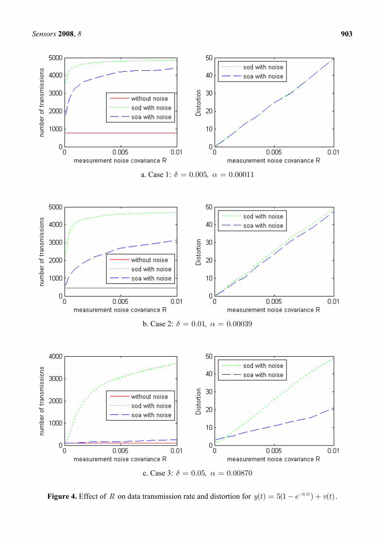
Figure 4. Effect of R on data transmission rate and distortion for y t .

Sensors 2008, 8

904

0.01s=α

R

It is very difficult to derive an explicit expression of signal distortion in two methods SOD and SOA by theoretical analysis because it depends not only on the given threshold but also the system model and noise. Thus, in this section we evaluate the effect of measurement noise on distortion by considering an example instead.

Consider two sensor outputs and , where R is varying. We will see how data transmission rate and distortion vary as R varies in both methods SOD and SOA. The evaluation is implemented with T in 50 seconds. The threshold values δ and

are given in 3 cases:

( ) 0.1 ( )y t t v t= + 0.1( ) 5(1 ) ( )ty t e v t−= − +

• Case 1. 0.005δ = : small threshold • Case 2. 0.01δ = : medium threshold • Case 3. 0.05δ = : large threshold

In the above example, α is chosen according to δ such that number of data transmissions in two methods is identical as (without noise). From the results in the Fig. 3 and Fig. 4, the effect of

on data transmission rate and distortion is summarized as follows: ( ) = 0v t

- When the threshold value is small as in case 1, distortion of SOA is equivalent to that of SOD but data transmission rate of SOA is smaller than that of SOD. In this case, using SOA will reduce data transmission rate.

- When the threshold value increases as in case 2, distortion of SOA is slightly smaller than that of SOD and data transmission rate of SOA is much smaller than that of SOD. In other words, we get benefit of data transmission rate reduction and a little distortion reduction from SOA method.

- When the threshold value is large as in case 3, SOA reduces not only data transmission rate but also distortion. The larger R value is, the more reduction is. This result is remarkable! It means that in the SOA method, signal distortion is not degraded along with the reduction of data transmission rate even when system noise is large. Therefore, we hope that estimation performance will be significantly improved when applying a filter.

3. State estimation with SOA Transmission method

The networked estimation problem applying SOA transmission method is depicted as follows: 1. Measurement outputs ( )1iy i≤ ≤ p are sampled at the period T but their data are only

transmitted to the estimator node when (3) is satisfied. 2. For simplicity in the problem formulation, transmission delay from the sensor nodes to the

estimator node is ignored. 3. The estimator node estimates states of the plant regularly at the period T regardless of whether

or not sensor data arrive. If there is no i -th sensor data received for > ,last it t , the estimator node considers that the measurement value of the i -th sensor output ( )iy t is still equal to ,last iy but the measurement noise increases from ( )iv t to )ast iv t t . = +( ) ( )n i iv t Δ ( , lt, ,i

To formulate a state estimation problem, the bound of needs to be determined. In the next section, we will compute the bound of and then a modified Kalman filter is applied for

state estimation.

,( , )i last it tΔ

,( , )i last it tΔ

Sensors 2008, 8

905

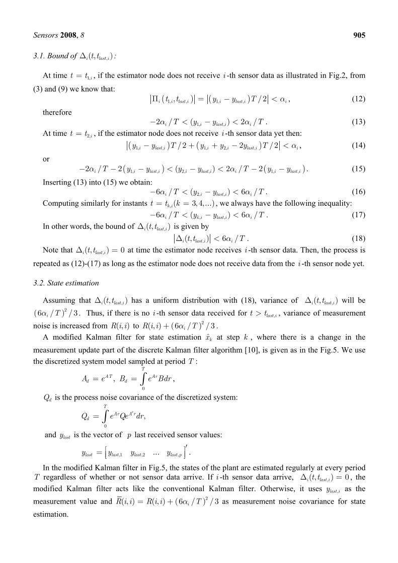
,( , )i last it t3.1. Bound of Δ :

At time , if the estimator node does not receive i -th sensor data as illustrated in Fig.2, from

(3) and (9) we know that: 1,it t=

( ) ( )1, , 1, ,,i i last i i last i it t y y T αΠ = − /2 <

α

, (12)

therefore 1, ,2 / ( ) 2 /i i last i iT y y Tα− < − < . (13)

At time , if the estimator node does not receive i -th sensor data yet then: 2,it t=

( ) ( )1, , 1, 2, ,/2 2 /2i last i i i last iy y T y y y T α− + + − i<

)

α

α

, (14)

or ( ) (1, , 2, , 1, ,2 / 2 ( ) 2 / 2i i last i i last i i i last iT y y y y T y yα α− − − < − < − − . (15)

Inserting (13) into (15) we obtain: 2, ,6 / ( ) 6 /i i last i iT y y Tα− < − < . (16)

Computing similarly for instants , we always have the following inequality: , ( 3, 4,...)k it t k= =

, ,6 / ( ) 6 /i k i last i iT y y Tα− < − < . (17) In other words, the bound of is given by ,( , )i last it tΔ

,( , ) 6 /i last i it t TαΔ < . (18) Note that at time the estimator node receives i -th sensor data. Then, the process is

repeated as (12)-(17) as long as the estimator node does not receive data from the i -th sensor node yet. ,( , ) 0i last it tΔ =

,( , )i last it t ,( , )i last it t

3.2. State estimation

Assuming that Δ has a uniform distribution with (18), variance of Δ will be ( )26 / /3i Tα > ,last i. Thus, if there is no i -th sensor data received for t t , variance of measurement noise is increased from to ( , )R i i ( )2) 6 / /3i Tα+

k

T

AT Ar r

dQ

Ar A rdr′

last

...y y y y ′⎡ ⎤=

T ,( , ) 0i last it t

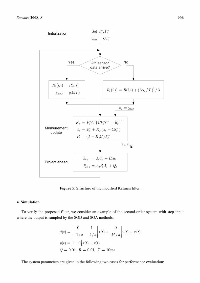
( ,iR i . A modified Kalman filter for state estimation at step , where there is a change in the

measurement update part of the discrete Kalman filter algorithm [10], is given as in the Fig.5. We use the discretized system model sampled at period T :

k̂x

0

, d dA e B e Bd= = ∫

T

,

is the process noise covariance of the discretized system:

0

,dQ e Qe= ∫

and y is the vector of p last received sensor values:

,1 ,2 ,last last last last p⎢ ⎥⎣ ⎦ .

In the modified Kalman filter in Fig.5, the states of the plant are estimated regularly at every period regardless of whether or not sensor data arrive. If i -th sensor data arrive, Δ = , the

modified Kalman filter acts like the conventional Kalman filter. Otherwise, it uses as the measurement value and

,last iy

( )2( , ) ( , ) 6 / /ii R i i Tα= + 3R i as measurement noise covariance for state estimation.

Sensors 2008

906, 8

( )( )

( )

1

ˆ ˆ ˆ

k k k k

k k k k k

k k k

K P C CP C R

x x K z Cx

P I K C P

−− −

− −

−

′ ′= +

= + −

= −

1

1

ˆ ˆk d k d k

k d k d d

x A x B u

P A P A Q

−+

−+

= +

′= +

k lastz y=

0 1ˆ ˆ, ,...x x

Project ahead

Measurement update

Initialization

i-th sensordata arrive?

0 0

0

ˆSet ,

ˆlast

x P

y Cx

− −

−=

Yes No

,

( , ) ( , )

( )

k

last i i

R i i R i i

y y kT

=

= ( )2( , ) ( , ) 6 / /3k iR i i R i i Tα= +

Figure 5. Structure of the modified Kalman filter.

4. Simulation

To verify the proposed filter, we consider an example of the second-order system with step input where the output is sampled by the SOD and SOA methods:

00 1⎡ ⎤

( ) ( ) ( ) ( )/1/ /

( ) 1 0 ( ) ( )

0.01, 0.01, 10

x t x t u t w tM aa b a

y t x t v t

Q R T ms

⎡ ⎤⎢ ⎥ ⎢ ⎥ += +⎢ ⎥ ⎢ ⎥− − ⎢ ⎥⎢ ⎥ ⎣ ⎦⎣ ⎦⎡ ⎤= +⎢ ⎥⎣ ⎦

= = =

The system parameters are given in the following two cases for performance evaluation:

Sensors 2008, 8

907

30, a 5= =

• Case 1. (underdampled system) 1= . 30, a 5, bM = =• Case 2. (undamped system) , b 0M = .

The simulation process is implemented for 50 seconds. In each case, we use two methods (SOD and SOA) for performance comparison. Estimation performance is evaluated by the average distortion:

( )22, , ,

1 1

ˆN N

i k i k i k ik k

D e x x= =

−∑ ∑ (i = i 5000N

0.9=

1 1N N

= = (19)

where e i is the estimation error, x is the reference state, and . 1,2)

α

=

The simulation results with different threshold values for the two cases are shown in Table 1 and Table 2, where value is chosen according to δ value such that n (number of sensor data transmissions) is identical in the two methods. In both cases, we see that when δ is small (i.e.

), estimation performance of SOD and SOA is almost the same. Rigorously speaking, SOD is slightly better than SOA. However, when δ is increasing, SOA method shows to be outperform significantly. For example as δ , SOA outperforms SOD by the

0.1, 0.3δ =

1D reduction of 5 times (i.e. 0.0116 vs. 0.0536 in case 1, and 0.0017 vs. 0.0081 in case 2). As illustrated in Fig. 6 and Fig. 7, the estimation error of SOA is much smaller than that of SOD.

Table 1. Estimation performance of 2 methods with different threshold values in case 1

δ 0.1 0.3 0.5 0.7 0.9

α 0.0006 0.0081 0.0302 0.0534 0.0881

n 2465 490 240 175 140

1D by SOD 6.08e-4 0.0026 0.0101 0.0268 0.0536

1D by SOA 6.40e-4 0.0030 0.0061 0.0103 0.0116

2D by SOD 0.0080 0.0106 0.0176 0.0205 0.0313

2D by SOA 0.0082 0.0110 0.0139 0.0144 0.0148

Table 2. Estimation performance of 2 methods with different threshold values in case 2

δ 0.1 0.3 0.5 0.7 0.9

α 0.0005 0.0038 0.0094 0.0181 0.0303

n 3347 1601 1094 822 658

1D by SOD 3.49e-4 8.94e-4 0.0022 0.0043 0.0081

1D by SOA 3.65e-4 8.32e-4 0.0015 0.0016 0.0017

2D by SOD 0.0052 0.0067 0.0087 0.0109 0.0131

2D by SOA 0.0053 0.0070 0.0079 0.0080 0.0080

Sensors 2008, 8 908

Figure 6. Estimation error as δ α in case 1 0.9, 0.0881= =

Figure 7. Estimation error as in case 2. 0.9, 0.0303δ α= =

Through simulation results, we see that the SOA method provides better estimation performance than the SOD method. The key reason is that in the SOD method, noise-containing sensor data not only make transmission rate increase but also degrade estimation performance. Whereas, thanks to the integral block which acts as a noise filter in the SOA sampling scheme, the sensor node does not send highly noisy data, but it transmits data only when the output indeed changes value. For that reason, the transmitted sensor data in the SOA method is more reliable. This helps estimation performance better.

5. Conclusion

In this paper, the state estimation problem with SOA transmission method over network has been considered. We have shown that when increasing the threshold value to improve bandwidth network, the SOA method gives much better estimation performance than the SOD method. This is very useful in the realistic applications where sensor data transmission rate needs to be lowered due to joining of many sensor nodes or for power saving in wireless networks. The SOA method has been also proven to be more efficient than the SOD method in the highly noisy systems.

Sensors 2008, 8

909

Acknowledgements

This work was supported by the Korea Science and Engineering Foundation (KOSEF) grant funded by the Korea government (MOST) (No. R01-2006-000-11334-0). The authors also would like to thank Ministry of Commerce, Industry and Energy and Ulsan Metropolitan City which partly supported this research through the Network-based Automation Research Center (NARC) at University of Ulsan.

References and Notes

1. Astrom, K.J.; Bernhardsson, B.M. Comparison of Riemann and Lebesgue sampling for first order stochastic systems. In Proceedings 41st Conference on Decision and Control; Las Vegas, U.S.A., 2002; pp 2011–2016.

2. Otanez, P.G.; Moyne, J.R.; Tilbury, D.M. Using deadbands to reduce communications in networked control systems. In Proceedings of the American Control Conference; Anchorage, U.S.A., 2002; pp 3015-3020.

3. Sandra, H.; Peter, H.; Eckehard, S.; Martin, B. Network Traffic Reduction in Haptic Telepresence Systems by Deadband Control. In Proceedings IFAC World Congress; International Federation of Automatic Control: Prague, Czech Republic, 2005.

4. Kofman, E.; Braslavsky, J.H. Level Crossing Sampling in Feedback Stabilization under Data-Rate Constraints. In Proceedings 45th Conference on Decision and Control; San Diego, U.S.A., 2006; pp 4423-4428.

5. Rabi, M.; Moustakides, G.V.; Baras, J.S. Multiple Sampling for Estimation on a Finite Horizon. In Proceedings 45th Conference on Decision and Control; San Diego, U.S.A., 2006; pp 1351-1357.

6. Mikowicz, M. Send-On-Delta Concept: An Event-Based Data Reporting Strategy. Sensors 2006, 65, 49-63.

7. Suh, Y.S.; Nguyen, V.H.; Ro, Y.S. Modified Kalman filter for networked monitoring systems employing a send-on-delta method. Automatica 2007, 43(2), 332-338.

8. Suh, Y.S. Send-On-Delta sensor data transmission with a linear predictor. Sensors 2007, 7, 537-547.

9. Mikowicz, M. Asymptotic Effectiveness of the Event-Based Sampling According to the Integral Criterion. Sensors 2007, 7, 16-37.

10. Brown, R.G.; and Hwang, P.Y.C. Introduction to Random Signals and Applied Kalman Filtering; John Wiley & Sons: New York, 1997.

11. Astrom, K. J. Introduction to Stochastic Control Theory; Academic Press: New York, 1970.

© 2008 by MDPI (http://www.mdpi.org). Reproduction is permitted for noncommercial purposes.