Signatures of anomalous VVH interactions at a linear collider

arX

iv:h

ep-p

h/05

0907

0v3

30

Jan

2007

IISc-CHEP/10/05hep-ph/0509070

Signatures of anomalous V V H interactions at a linear collider

Sudhansu S. Biswal1,∗, Debajyoti Choudhury2,†, Rohini M. Godbole1,‡, and Ritesh K. Singh1,§

1Center for High Energy Physics,

Indian Institute of Science, Bangalore, 560012, India

2Department of Physics and Astrophysics,

University of Delhi, Delhi 110007, India

and

HarishChandra Research Institute,

Chhatnag Road, Jhusi, Allahabad 211019, India

We examine, in a model independent way, the sensitivity of a Linear Collider to the couplings ofa light Higgs boson to gauge bosons. Including the possibility of CP violation, we construct severalobservables that probe the different anomalous couplings possible. For an intermediate mass Higgs,a collider operating at a center of mass energy of 500 GeV and with an integrated luminosity of500 fb−1 is shown to be able to constrain the ZZH vertex at the few per cent level, and with evenhigher sensitivity in certain directions. However, the lack of sufficient number of observables as wellas contamination from the ZZH vertex limits the precision with which the WWH coupling can bemeasured.

PACS numbers: 14.80.Cp, 14.70.FM, 14.70.Hp

I. INTRODUCTION

Although the standard model (SM) has withstood allpossible experimental challenges and has been testedto an unprecedented degree of accuracy, so far therehas been no direct experimental verification of the phe-nomenon of spontaneous symmetry breaking. With thelatter being considered a central pillar of this theory andits various extensions, the search for a Higgs boson is oneof the main aims for many current and future colliders [1].Within the SM, the only fundamental spin-0 object is the(CP -even) Higgs boson and remains the only particle inthe SM spectrum to be found yet. Rather, a lower boundon the mass of the SM Higgs boson, (about 114.5 GeV)is provided by the direct searches at the LEP collider [2].Electroweak precision measurements, on the other hand,provide an upper bound on its mass of about 204 GeV at95% C.L. [3]. It should be realized that both these limitsare model dependent and may be relaxed in extensionsof the SM. For example, the lower limit can be relaxedin generic 2-Higgs doublet models [4] or in models withCP violation [5]. In the latter case, direct searches atLEP and elsewhere still allow the lightest Higgs boson tobe as light as 10 GeV [6]. Similarly, the upper bound onthe mass of the (lightest) Higgs in some extensions maybe substantially higher [7]. The Large Hadron Collider(LHC) is expected to be capable [8] of searching for theHiggs boson in the entire mass range allowed.

It is then quite obvious that just the discovery of theHiggs boson at the LHC will not be sufficient to validate

∗Electronic address: [email protected]†Electronic address: [email protected]‡Electronic address: [email protected]§Electronic address: [email protected]

the minimal SM. For one, the only neutral scalar in theSM is a JCP = 0++ state arising from a SU(2)L doubletwith hypercharge 1, while its various extensions can haveseveral Higgs bosons with different CP properties andU(1) quantum numbers. The minimal supersymmetricstandard model (MSSM), for example, has two CP -evenstates and a single CP -odd one [9]. Thus, should a neu-tral spin-0 state be observed at the LHC, a study of itsCP -property would be essential to establish it as the SMHiggs boson [10].

Since, at an e+e− collider, the dominant productionmodes of a neutral Higgs boson proceed via its cou-pling with a pair of gauge bosons (V V, V = W, Z), anychange in the V V H couplings from their SM values canbe probed via such production processes. Within theSM/MSSM, the only (renormalizable) interaction terminvolving the Higgs boson and a pair of gauge bosonsis the one arising from the Higgs kinetic term. How-ever, once we accept the SM to be only an effective low-energy description, higher-dimensional (and hence non-renormalizable) terms are allowed. If we only demandLorentz invariance and gauge invariance, the most gen-eral coupling structure may be expressed as

Γµν = gV

[aV gµν +

bV

m2V

(k1νk2µ − gµν k1 · k2)

+bV

m2V

ǫµναβ kα1 kβ

2

](1)

where ki denote the momenta of the two W ’s (Z’s),gSM

W = e cot θW MZ and gSMZ = 2 e MZ/ sin 2θW . In

the context of the SM, at the tree level, aSMW = aSM

Z = 1while the other couplings vanish identically. At the one-loop level or in a different theory, effective or otherwise,these may assume significantly different values. We studythis most general set of anomalous couplings of the Higgs

http://arXiv.org/abs/hep-ph/0509070v3

2

boson to a pair of W s and Z at a linear collider (LC) inthe processes e+e− → f fH , with f being a light fermion.

The various kinematical distributions for the processe+e− → f fH , proceeding via vector boson fusion andHiggsstrahlung, with unpolarized beams has been stud-ied in the context of the SM [11]. The effect of beampolarization has also been investigated for the SM [12].The anomalous ZZH couplings have been studied inRefs.[13, 14, 15, 16, 17] for the LC and in Refs.[18, 19]for the LHC in terms of higher dimensional operators.Ref. [20] investigates the possibility to probe the anoma-lous V ZH couplings, V = γ, Z, using the optimal observ-able technique [21] for both polarized and un-polarizedbeams. Ref. [22], on the other hand, probes the CP -

violating coupling bZ by means of asymmetries in kine-matical distributions and beam polarization. In Ref. [23],the V V H vertex is studied in the process of γγ → H →W+W−/ZZ using angular distributions of the decayproducts.

The rest of the paper is organized as follows. In sec-tion II we discuss the possible sources and symmetriesof the anomalous V V H couplings and the rates of vari-ous processes involving these couplings. In section III weconstruct several observables with appropriate CP andT property to probe various ZZH anomalous couplings.In section IV we construct similar observables to probeanomalous WWH couplings, which we then use alongwith the ones constructed for the ZZH case. Section Vcontains a discussion and summary of our findings.

II. THE V V H COUPLINGS

The anomalous V V H couplings in Eq.(1) can appearfrom various sources such as via higher order correctionsto the vertex in a renormalizable theory [24] or fromhigher dimensional operators in an effective theory [25].For example, in the MSSM, the non-zero phases of thetrilinear SUSY breaking parameter A and the gaug-ino/higgsino mass parameters can induce CP -violatingterms in the scalar potential at one loop level even thoughthe tree level potential is CP -conserving. As a conse-quence, the Higgs-boson mass eigenstates can turn outto be linear combinations of CP -even and -odd states.This modifies the effective coupling of the Higgs bosonto the known particles from what is predicted in the SM(or even from that within a version of MSSM with noCP -violation accruing from the scalar sector).

In a generic multi-doublet model, whether supersym-metric [26] or otherwise [27], the couplings of the neutralHiggs bosons to a pair of gauge bosons satisfy the sumrule

∑

i

a2V V Hi

= 1.

Thus, while aV V Hifor a given Higgs boson can be sig-

nificantly smaller than the SM value, any violation ofthe above sum rule would indicate either the presenceof higher SU(2)L multiplets or more complicated sym-metry breaking structures (such as those within higher-

dimensional theories) [27]. The couplings bV or bV

e�e+

VV f�f H(a) e�

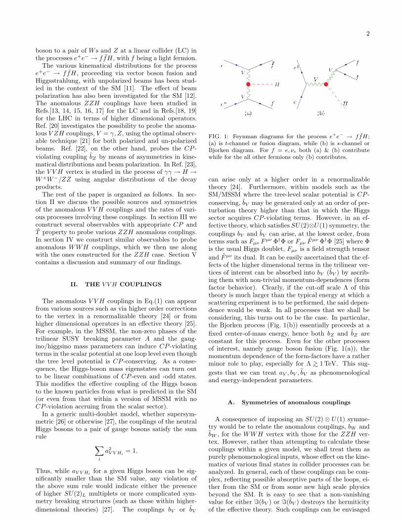
e+ V V f�fH(b)FIG. 1: Feynman diagrams for the process e+e− → ffH ;(a) is t-channel or fusion diagram, while (b) is s-channel orBjorken diagram. For f = e, νe both (a) & (b) contributewhile for the all other fermions only (b) contributes.

can arise only at a higher order in a renormalizabletheory [24]. Furthermore, within models such as theSM/MSSM where the tree-level scalar potential is CP -

conserving, bV may be generated only at an order of per-turbation theory higher than that in which the Higgssector acquires CP -violating terms. However, in an ef-fective theory, which satisfies SU(2)⊗U(1) symmetry, the

couplings bV and bV can arise, at the lowest order, fromterms such as Fµν Fµν Φ†Φ or Fµν Fµν Φ†Φ [25] where Φis the usual Higgs doublet, Fµν is a field strength tensor

and Fµν its dual. It can be easily ascertained that the ef-fects of the higher dimensional terms in the trilinear ver-tices of interest can be absorbed into bV (bV ) by ascrib-ing them with non-trivial momentum-dependences (formfactor behavior). Clearly, if the cut-off scale Λ of thistheory is much larger than the typical energy at which ascattering experiment is to be performed, the said depen-dence would be weak. In all processes that we shall beconsidering, this turns out to be the case. In particular,the Bjorken process (Fig. 1(b)) essentially proceeds at a

fixed center-of-mass energy, hence both bZ and bZ areconstant for this process. Even for the other processesof interest, namely gauge boson fusion (Fig. 1(a)), themomentum dependence of the form-factors have a ratherminor role to play, especially for Λ >∼ 1 TeV. This sug-

gests that we can treat aV , bV , bV as phenomenologicaland energy-independent parameters.

A. Symmetries of anomalous couplings

A consequence of imposing an SU(2) ⊗ U(1) symme-try would be to relate the anomalous couplings, bW andbW , for the WWH vertex with those for the ZZH ver-tex. However, rather than attempting to calculate thesecouplings within a given model, we shall treat them aspurely phenomenological inputs, whose effect on the kine-matics of various final states in collider processes can beanalyzed. In general, each of these couplings can be com-plex, reflecting possible absorptive parts of the loops, ei-ther from the SM or from some new high scale physicsbeyond the SM. It is easy to see that a non-vanishingvalue for either ℑ(bV ) or ℑ(bV ) destroys the hermiticityof the effective theory. Such couplings can be envisaged

3

TABLE I: Transformation properties of various anomalouscouplings under discrete transformations.

Trans. aV ℜ(bV ) ℑ(bV ) ℜ(bV ) ℑ(bV )CP + + + − −

T + + − − +

when one goes beyond the Born approximation, whencethey arise from final state interactions, or, in other words,out of the absorptive part(s) of higher order diagrams,presumably mediated by new physics. A fallout of non-hermitian transition matrices is non-zero expectation val-ues of observables which are odd under CPT , where Tstands for the pseudo-time reversal transformation, onewhich reverses particle momenta and spins but does notinterchange initial and final states. Of course, such non-zero expectation values will be indicative of final stateinteraction only when kinematic cuts are such that thephase space integration respects CPT . Note that aV toocan be complex in general and can give an additionalT -odd contribution. However, for the processes that wewill consider, the phase of at least one of aW and aZ canalways be rotated away, and we make this choice for aZ .Henceforth, we shall assume that aW and aZ are close to

their SM value, i.e. ai = 1+∆ai, the rationale being thatany departure from aSM

W and aSMZ respectively would be

the easiest to measureUnfortunately, this still leaves us with many free pa-

rameters making an analysis cumbersome. One mightargue that SU(2)⊗U(1) gauge invariance would predict∆aW = ∆aZ . However, once symmetry breaking effectsare considered, this does not necessarily follow [24]. Nev-ertheless, we will make this simplifying assumption that∆aW is real and equal to ∆aZ , i.e. aW = aZ , since theequality is found to hold true in some specific cases [28](and would be dictated if SU(2) ⊗ U(1) were to be anexact symmetry of the effective theory). With this as-

sumption, we list, in Table I, the CP and T propertiesof such operators.

Finally, keeping in view the higher-dimensional natureof all of these couplings, we retain only contributions upto the lowest non-trivial order, arising from terms linearin the additional couplings.

B. Cross-sections

The dominant channels of Higgs production at anelectron-positron colliders are

1. the 2-body Bjorken process (e+e− → ZH);

2. in association with a pair of neutrinos (e+e− →νeνeH), i.e. W -fusion;

3. in association with an e+e− pair (e+e− → e+e−H),i.e. Z-fusion

Note that the Bjorken-process also contributes to theother two final states through the subsequent decay of

the Z. Of these three, the e+e−H channel is consid-erably suppressed (by almost a factor of 10) with re-spect to the νeνeH channel over a very wide range ofcenter-of-mass energies (

√s) and Higgs masses. As can

be expected, at large√

s, the Bjorken process suffers theusual s-channel suppression and has a smaller cross sec-tion compared to that for W/Z-fusion. In fact, even for√

s = 500 GeV and unpolarized beams, the Bjorken pro-cess dominates over W -fusion only for relatively largeHiggs masses [29, 30, 31].

In view of this, it might seem useful to concentratefirst on the dominant channel, viz e+e− → ννH andthereby constrain bW and bW . However, it is immedi-ately obvious that the Bjorken process too contributesto this final state and hence the couplings ∆aZ , bZ andbZ have a role to play. Since the total rate is a CP -even(as well as T even) observable, it can receive contributiononly from ℜ(bV ). [Note that a non-zero ∆aV would onlyrescale the SM rates.] The other non-standard couplings,

odd under CP and/or T , are responsible for various po-lar and azimuthal asymmetries and contribute nothingto the total rate on integration over a symmetric phasespace[35]. This can be understood best by consideringthe square of the invariant amplitude pertaining to on-shell Z-production, namely e+e− → ZH :

|M|2 ∝ |aZ |2ℓ2e + r2

e

4

[1 +

E2Z − p2 cos2 θ

m2Z

]

+ℜ(aZ b∗Z)

m2Z

(ℓ2e + r2

e)√

s EZ

+ℑ(aZ b∗Z)

m2Z

(ℓ2e − r2

e)√

s p cos θ

(2)

with ℓe(re) denoting the electron’s couplings to the Z,and EZ , p, θ the energy, momentum and scattering an-gle of the Z in the c.m.-frame. The proportionalityconstant includes, alongwith the couplings etc., a factors/[(s−m2

Z)2+Γ2Zm2

Z ]. This suggests that the anomalouscontribution vanishes for large s, inspite of the higher-dimensional nature of the coupling. Furthermore, Eq.(2)

also demonstrates that neither ℑ(bZ) nor ℜ(bZ) maymake their presence felt if the polarization of the Z couldsimply be summed over. It also shows that the contribu-tion due to ℑ(bZ) would disappear when integrated overa symmetric part of the phase space as has been men-tioned before. Thus, if we want to probe these couplings,we would need to look at rates integrated only over par-tial (non-symmetric) phase space. As an example, letus consider the forward-backward asymmetry for the Z-boson. As can be seen from Eq.(2), it is proportional to

ℑ(bZ) alone. This can be understood by realizing thatthis observable is proportional to the expectation valueof (~pe · ~pZ) and hence is a CP -odd and T -even quantity

just as ℑ(bZ) is. For ℑ(bZ) and ℜ(bZ), which are T -odd, one has to look at the azimuthal correlations of thefinal state fermions. Equivalently one can look for par-tial cross-section, restricting the azimuthal angles overa given range. A discussion of how partial cross-sectioncan be used to probe anomalous couplings is given inAppendix A. Further, Eq.(2) also indicates that the an-gular distribution of the Higgs (or, equivalently, that of

4

the Z) is different for the SM piece than that for the pieceproportional to ℜ(bZ); the difference getting accentuatedat higher

√s. This, in principle, could be exploited to

increase the sensitivity to ℜ(bZ).In this paper we restrict ourselves to the case of a first

generation linear collider. For such√

s, the interferencebetween the W -fusion diagram with the s-channel one isenhanced for non-zero bZ and bZ . At a first glance, itmay seem that the kinematic difference between the twoset of diagrams could be exploited and the two contribu-tions separated from each other with some simple cuts.However, in actuality, such a simple approach does notsuffice to adequately decouple them. It is thus contin-gent upon us to first constrain the non-standard ZZHcouplings from processes that involve just these and onlythen to attempt to use WW -fusion process to probe theWWH vertex.

III. THE ZZH COUPLINGS

The anomalous ZZH couplings have been studied ear-lier in the process e+e− → f fH in the presence of ananomalous γγH coupling [20] making use of optimal ob-servables [21]. The CP -violating anomalous ZZH cou-plings alone have also been studied in Ref. [22], whichconstructs asymmetries for both polarized and unpo-larized beams. We, however, choose to be conserva-tive and restrict ourselves to unpolarized beams. And,rather than advocating the use of complicated statis-tical methods, we construct various simple observablesthat essentially require only counting experiments. Fur-thermore, we include the decay of the Higgs boson, ac-count for b-tagging efficiencies and kinematical cuts toobtain more realistic sensitivity limits. Since we are pri-marily interested in the intermediate mass Higgs boson(2mb ≤ mH ≤ 140 GeV), H → bb is the dominant decaymode with a branching fraction >∼ 0.9.

A. Kinematical Cuts

For a realistic study of the process e+e− → f fH(bb),we choose to work with a Higgs boson of mass 120 GeVand a collider center-of-mass energy of 500 GeV. To en-sure detectability of the b-jets, we require, for each, aminimum energy and a minimum angular deviation fromthe beam pipe. Furthermore, the two jets should be wellseparated so as to be recognizable as different ones. Tobe quantitative, we require that

Eb, Eb ≥ 10 GeV,

5◦ ≤ θb, θb ≤ 175◦

∆Rbb ≥ 0.7

(3)

where (∆R)2 ≡ (∆φ)2+(∆η)2 with ∆φ and ∆η denotingthe separation between the two b-jets in azimuthal angleand rapidity respectively.

For events with the Z decaying into a pair of leptonsor light quarks, we have similar demands on the latter,

namely

Ef , Ef ≥ 10 GeV, 5◦ ≤ θf , θf ≤ 175◦. (4)

For leptons, i.e. f = ℓ, we require a lepton–lepton sepa-ration:

∆Rℓ−ℓ+ ≥ 0.2 (5)

along with a b−jet–lepton isolation:

∆Rbℓ ≥ 0.4 (6)

for each of the four jet-lepton pairings. For f = q, i.e.light quarks, we impose, instead,

∆Rq1q2≥ 0.7 (7)

for each of the six pairings. On the other hand, if the Zwere to decay into neutrinos, the requirements of Eqs.(4–7) are no longer applicable and instead we demand thatthe events contain only the two b-jets along with a mini-mum missing transverse momentum, viz

pmissT ≥ 15 GeV . (8)

The above set of cuts select the events corresponding tothe process of interest, rejecting most of the QED-drivenbackgrounds. To further distinguish between the roleof the Bjorken diagram and that due to the ZZ (WW )fusion in the case of e+e−H (ννH) final state we need toselect/de-select the events corresponding to the Z-masspole. This is done via an additional cut on the invariantmass of f f , viz.

R1 ≡∣∣mff − MZ

∣∣ ≤ 5 ΓZ select Z-pole ,

R2 ≡∣∣mff − MZ

∣∣ ≥ 5 ΓZ de-select Z-pole.(9)

Since an exercise such as the current one would be un-dertaken only after the Higgs has been discovered andits mass measured to a reasonable accuracy, one mayalternatively demand that the energy of the Higgs (re-constructed bb pair) is close to (s + m2

H − m2Z)/(2

√s),

namely

R1′ ≡ E−H ≤ EH ≤ E+

H

R2′ ≡ EH < E−H or EH > E+

H

(10)

where E±H = (s + m2

H − (mZ ∓ 5ΓZ)2)/(2√

s). This hasthe advantage of being applicable to the ννH final stateas well. The b-jet tagging efficiency is taken to be 0.7.We add the statistical error and a presumed 1% system-atic error (accruing from luminosity measurements etc.)in quadrature. In other words, the fluctuation in themeasurement of a cross-sections is assumed to be

∆σ =√

σSM/L + ǫ2σ2SM , (11)

while that for an asymmetry is

(∆A)2 =1 − A2

SM

σSML +ǫ2

2(1 − A2

SM )2. (12)

5

Here σSM is the SM value of cross-section, L is the inte-grated luminosity of the e+e− collider and ǫ is the frac-tional systematic error. Since we work in the linear ap-proximation for the anomalous couplings, any observable,rate or asymmetry, can be written as

O({Bi}) =∑

Oi Bi.

Then we define the blind region as the region in the pa-rameter space for which

|O({Bi}) −O({0})| ≤ f δO, (13)

where f is the degree of statistical significance, O({0}) isthe SM value of O and δO is the statistical fluctuation inO. All the limits and blind regions quoted in this paperare obtained using the above relation. Note that in allthe cases that we will consider, the asymmetries vanishidentically within the SM.

B. Cross-sections

The simplest observable, of course, is the total rate.Note that ℑ(bZ), inspite of being T -odd, does result in anon-zero, though small, contribution to the total cross-section. This is but a consequence of the absorptive partin the propagator and would have been identically zeroin the limit of vanishing widths. Since we retain con-tributions to the cross-section that are at best linear inthe couplings, the major non-trivial anomalous contribu-tion, on imposition of the R1 cut, emanates from ℜ(bZ)with only subsidiary contributions from ℑ(bZ). For ourdefault choice (a 120 GeV Higgs at a machine operatingat

√s = 500 GeV), on selecting the Z-pole (R1 cut) the

rates, in femtobarns, are

σ(e+e−) = 1.28 + 12.0 ℜ(bZ) + 0.189 ℑ(bZ)

σ(µ+µ−) = 1.25 + 11.9 ℜ(bZ)

σ(uu/cc) = 2 [4.25 + 40.2 ℜ(bZ)]

σ(dd/ss) = 2 [5.45 + 51.6 ℜ(bZ)]

(14)

On de-selecting the Z-pole (R2 cut) we obtain, instead

σ(e+e−) = [4.76 − 0.147 ℜ(bZ)] fb. (15)

The total rates, by themselves, may be used to put strin-gent constraints on ℜ(bZ). For Z decaying into lightquarks and µs (with the R1 cut) and for an integratedluminosity of 500 fb−1, the lack of any deviation from theSM expectations would give

|ℜ(bZ)| ≤ 0.44 × 10−2 (16)

at the 3σ level. We do not use the e+e−H final statein deriving the above constraint as it receives a contri-bution proportional to ℑ(bZ) too. This arises from theinterference of the Bjorken diagram with the ZZ-fusiondiagram due to the presence of the absorptive part in thenear-on-shell Z-propagator.

The cross-sections shown in Eqs.(14 & 15) and the con-straint of Eq.(16) have been derived assuming the SMvalue for aZ . Clearly, any variation in aZ would affect

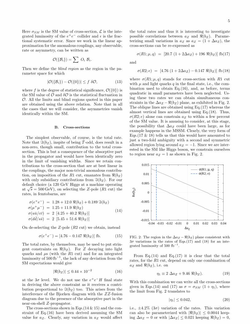
the total rates and thus it is interesting to investigatepossible correlations between aZ and ℜ(bZ). Parame-terizing small variations in aZ as aZ = (1 + ∆aZ), thecross-sections can be re-expressed as

σ(R1; µ, q) = [20.7 (1 + 2∆aZ) + 196 ℜ(bZ)] fb(17)

and

σ(R2; e) = [4.76 (1 + 2∆aZ) − 0.147 ℜ(bZ)] fb (18)

where σ(R1; µ, q) stands for cross-section with R1 cutwith µ and light quarks q in the final state, i.e., the com-bination used to obtain Eq.(16), and, as before, termsquadratic in small parameters have been neglected. Us-ing these two rates we can obtain simultaneous con-straints in the ∆aZ −ℜ(bZ) plane, as exhibited in Fig. 2.The oblique lines are obtained using Eq.(17) whereas thealmost vertical lines are obtained using Eq.(18). Thus,σ(R2; e) alone can constrain aZ to within a few percentof the SM value. It is amusing to consider, at this stage,the possibility that ∆aZ could have been large, as forexample happens in the MSSM. Clearly, the very form ofEqs.(17 & 18) tells us that this would have amounted tojust a two-fold ambiguity with a second and symmetricallowed region lying around aZ = −1. Since we are inter-ested in the SM like Higgs boson, we constrain ourselvesto region near aZ = 1 as shown in Fig. 2.

-0.015

-0.01

-0.005

0

0.005

0.01

0.015

-0.04 -0.03 -0.02 -0.01 0 0.01 0.02 0.03 0.04

Re(

b Z)

∆aZ

σ(R1; µ, q)σ(R2; e)

FIG. 2: The region in the ∆aZ −ℜ(bZ) plane consistent with3σ variations in the rates of Eqs.(17) and (18) for an inte-grated luminosity of 500 fb−1.

From Eq.(14) and Eq.(17) it is clear that the totalrates, for the R1 cut, depend on only one combination ofaZ and ℜ(bZ), i.e. on

η1 ≡ 2 ∆aZ + 9.46 ℜ(bZ). (19)

With this combination we can write all the cross-sectionsgiven in Eqs.(14) and (17) as σ = σSM (1 + η1), wherethe limit from Fig. 2 translates to

|η1| ≤ 0.042, (20)

i.e., ±4.2% (3σ) variation of the rates. This variationcan also be parameterized with |ℜ(bZ)| ≤ 0.0044 keep-ing ∆aZ = 0 or with |∆aZ | ≤ 0.021 keeping ℜ(bZ) = 0,

6

(i.e., the intercepts of the solid lines in Fig. 2 on the y–and x–axes respectively). In other words, the individuallimit, i.e. the limit obtained keeping only one anoma-lous coupling non-zero, on ℜ(bZ) is 0.0044 and that on∆aZ is 0.021. On the other hand, if the R2 cut wereto be operative, we obtain the constraint |∆aZ | ≤ 0.034almost independent of ℜ(bZ), see Fig. 2. This constrainttranslates to a ±6.8% (3σ) variation in the rate σ(R2; e).

Note that the contributions proportional to the absorp-tive part of the Z-propagator are proportional to ΓZ awayfrom the resonance, i.e. for the R2 cut. Hence in this caseit is a higher order effect and thus ignored in Eqs.(15)and (18). On the other hand, near the Z-resonance theseterms are proportional to 1/ΓZ and hence of the sameorder in the perturbation theory. Thus, in order to beconsistent at a given order in the coupling αem we retainthese contribution only with the R1 cut.

C. Forward-backward asymmetry

The final state constitutes of two pairs of identifiableparticles : bb coming from the decay of Higgs boson andf f , where f 6= b. One can define forward-backwardasymmetry with respect to all the four fermions. Butwe choose, among them, the asymmetries with definitetransformation properties under CP and T . In thepresent case we have only one such forward-backwardasymmetry, i.e. the expectation value of (~pe− − ~pe+) ·(~pf + ~pf ). In other words, it is the forward-backwardasymmetry with respect to the polar angle of the Higgsboson (up to an overall sign) and given as

AFB(cos θH) =σ(cos θH > 0) − σ(cos θH < 0)

σ(cos θH > 0) + σ(cos θH < 0). (21)

This observable is CP odd and T even, and hence a probepurely of of ℑ(bZ) [see Table I]. Note that this asym-metry is proportional to (r2

e − l2e), where re (le) are theright-(left-) handed couplings of the electron to the Z-boson. With the R1 cut—see Eq.(9)—operative, a semi-analytical expression for this asymmetry, keeping onlyterms linear in the anomalous couplings, is given by

AFB(cH) =

0.059 ℜ(bZ) − 1.22 ℑ(bZ)

1.28(e+e−)

−1.2 ℑ(bZ)

1.25(µ+µ−)

−18.5 ℑ(bZ)

19.4(qq)

(22)In the above, “q” stands for all four flavors of light quarkssummed over and cH ≡ cos θH . Note here, that the con-tribution to the denominator of Eq.(21) from the anoma-lous terms have been dropped as the formalism allows usto retain terms only upto the first order in these cou-plings. In any case, their presence would have had onlya miniscule effect on the ensuing bounds. The asymme-try corresponding to the R2 cut is very small and is notconsidered. Omitting the (e+e−) final state on account

of the presence of ℜ(bZ), we use only the light quarks

and µs. For an integrated luminosity of 500 fb−1, thecorresponding 3σ limit is

|ℑ(bZ)| ≤ 0.038. (23)

-1.2

-1

-0.8

-0.6

-0.4

-0.2

0

0.2

0.4

0.6

0.8

1

1.2

-1 -0.8 -0.6 -0.4 -0.2 0 0.2 0.4 0.6 0.8 1

dσ/d

cosθ

cosθ

SM

Im(∼bZ)

e+e−→ e+e− H (R1 cut)

cH

cb

cH

cb

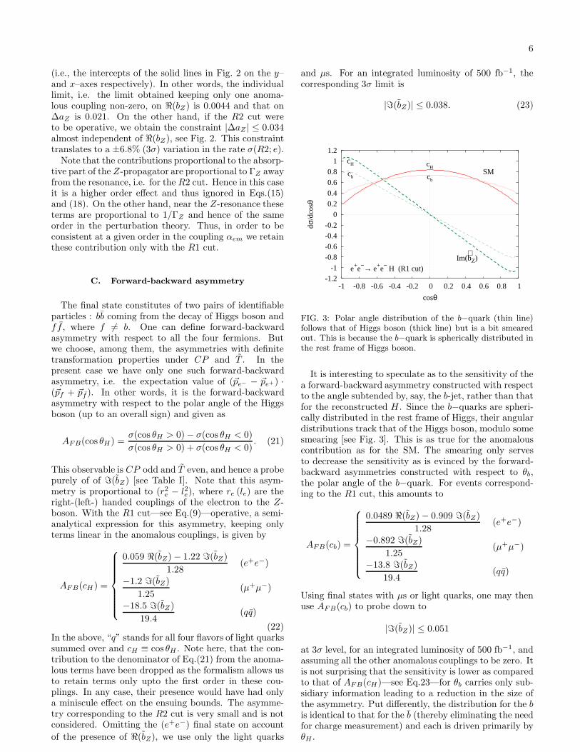
FIG. 3: Polar angle distribution of the b−quark (thin line)follows that of Higgs boson (thick line) but is a bit smearedout. This is because the b−quark is spherically distributed inthe rest frame of Higgs boson.

It is interesting to speculate as to the sensitivity of thea forward-backward asymmetry constructed with respectto the angle subtended by, say, the b-jet, rather than thatfor the reconstructed H . Since the b−quarks are spheri-cally distributed in the rest frame of Higgs, their angulardistributions track that of the Higgs boson, modulo somesmearing [see Fig. 3]. This is as true for the anomalouscontribution as for the SM. The smearing only servesto decrease the sensitivity as is evinced by the forward-backward asymmetries constructed with respect to θb,the polar angle of the b−quark. For events correspond-ing to the R1 cut, this amounts to

AFB(cb) =

0.0489 ℜ(bZ) − 0.909 ℑ(bZ)

1.28(e+e−)

−0.892 ℑ(bZ)

1.25(µ+µ−)

−13.8 ℑ(bZ)

19.4(qq)

Using final states with µs or light quarks, one may thenuse AFB(cb) to probe down to

|ℑ(bZ)| ≤ 0.051

at 3σ level, for an integrated luminosity of 500 fb−1, andassuming all the other anomalous couplings to be zero. Itis not surprising that the sensitivity is lower as comparedto that of AFB(cH)—see Eq.23—for θb carries only sub-sidiary information leading to a reduction in the size ofthe asymmetry. Put differently, the distribution for the bis identical to that for the b (thereby eliminating the needfor charge measurement) and each is driven primarily byθH .

7

Note that we have desisted from using the non-zeroforward-backward asymmetry in the polar angle distri-bution of f(f). Such observables do not have the requi-site CP -properties and are, in fact, non-zero even withinthe SM. The presence of non-zero ℑ(bZ) provides only anadditional source for the same and the limits extractablewould be weaker than those we have obtained.

D. Up-down asymmetry

The Higgs being a spin–0 object, its decay products areisotropically distributed in its rest frame. This, however,is not true of the Z. Still, CP conservation ensures thatthe leptons from Z decay are symmetrically distributedabout the plane of production. Thus, an up-down asym-metry defined as

AUD(φ) =σ(sin φ > 0) − σ(sin φ < 0)

σ(sin φ > 0) + σ(sin φ < 0)(24)

can be non-zero for the anomalous couplings. Inother words, a non-zero expectation value for[(~pe− − ~pe+) × ~pH ] · (~pf − ~pf ) is a CP odd (and Todd) observable. In our notation, it is driven by the non-

zero real part of bZ , and, for our choice of parameters,amounts to

AUD(φe−) =−0.354 ℜ(bZ) − 0.226 ℑ(bZ)

1.28

AUD(φµ−) =−0.430 ℜ(bZ)

1.25

AUD(φu) =−4.62 ℜ(bZ)

4.25

AUD(φd) =−7.98 ℜ(bZ)

5.45

(25)

up to linear order in the anomalous couplings. In obtain-ing Eq.25, the R1 cut has been imposed on the f f invari-ant mass. Note that, except for the e+e−H final state,AUD is a probe purely of ℜ(bZ). The cross section for thee+e−H final state receives additional contribution fromℑ(bZ) due to the absorptive part of the Z-propagator inthe Bjorken diagram. Although AUD(φu) and AUD(φd)

offer much larger sensitivity to ℜ(bZ) than do either ofAUD(φe−) and AUD(φµ−), the former can not be usedas the measurement of such asymmetries requires chargedetermination for light quark jets. However, one can de-termine the charge of b-quarks [32] and using AUD(φb),for the b’s resulting from the Z decay, we may obtain, foran integrated luminosity of 500 fb−1, a 3σ bound of

|ℜ(bZ)| ≤ 0.042

with 100% charge determination efficiency and only

|ℜ(bZ)| ≤ 0.089

if the efficiency were 20%. Note though that the Z → bbfinal state is beset with additional experimental com-plications (such as final state combinatorics) than thesemileptonic channels and hence we would not consider

this in deriving our final limits. Note that we do not ac-count for any combinatorics in obtaining the above saidlimits. However, we argue that the invariant masses ofthe bb pair coming from Z and H are non-overlappinghence the change in the above limits due to combina-torics are expected to be small.

Another obvious observable is AUD(φµ−). Using this,an integrated luminosity of 500 fb−1, would lead to a 3σconstraint of

ℜ(bZ)| ≤ 0.35. (26)

The reduced sensitivity of the Z → µ+µ− channel ascompared to the Z → bb channel is easy to understand.As Eq.(B5) demonstrates, AUD(φf ) ∝ (r2

e − ℓ2e) (r2

f − ℓ2f).

Since |rµ| ≈ |ℓµ|, this naturally leads to an additionalsuppression for AUD(φµ− ).

For the e+e−H case, on the other hand, the ZZ-fusiondiagram leads to a contribution that is proportional to(r2

e + ℓ2e)

2 and is, thus, unsuppressed. Accentuating thiscontribution by employing the R2 cut on mee, we have

AR2UD(φe− ) =

5.48 ℜ(bZ)

4.76(27)

and this, for an integrated luminosity of 500 fb−1, leadsto a 3σ constraint of

|ℜ(bZ)| ≤ 0.057. (28)

Here we note that the limit on ℜ(bZ), obtained using theR2 cut given above, is much better than the one obtainedusing R1 cut in Eq.(26), or even the one derived from the4 b final state assuming a 20% charge detection efficiency.

E. Combined polar and azimuthal asymmetries

Rather than considering individual asymmetries in-volving the (partially integrated) distributions in eitherof the polar or the azimuthal angle, one may attempt tocombine the information in order to potentially enhancethe sensitivity. To this end, we define a momentum cor-relation of the form

C1 =[(~pe− − ~pe+) · ~pµ−

][[(~pe− − ~pe+) × ~pH ] · (~pµ− − ~pµ+)

], (29)

where the sign of the term in the first square bracket de-cides if the µ− is in forward(F ) hemisphere with respectto the direction of e− or backward(B). Similarly, thesign of the term in second square bracket defines if µ− isabove(U) or below(D) the Higgs production plane. Thusthe expectation value of the sign of this correlation issame as the combined polar-azimuthal asymmetry givenby,

A(θµ, φµ) =(FU) + (BD) − (FD) − (BU)

(FU) + (BD) + (FD) + (BU)

=0.659 ℑ(bZ) − 0.762 ℜ(bZ)

1.25(30)

with the second equality being applicable for the R1 cut.In the above, (FU) is the partial cross-sections for µ− in

8

the forward-up direction and so on for others. Note thatC1 is T -odd but does not have a definite CP and hencedepends on both the T -odd couplings as seen in Eq.(30).We do not consider the analogous asymmetry for qqHfinal state as it demands charge determination for lightquarks (although Z → bb may be considered profitably).Similarly, for the e+e−H final state, A(θe, φe) receives

contributions from T -even couplings as well and hencenot considered for the analysis.

-0.3

-0.2

-0.1

0

0.1

0.2

0.3

-0.06 -0.04 -0.02 0 0.02 0.04 0.06

Im(b

Z)

Re(∼bZ)

Acom [e + µ ]

A(θµ,φµ)

AR2UD(φe)

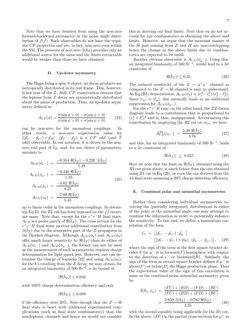
FIG. 4: Region in ℜ(bZ) −ℑ(bZ) plane corresponding to the3σ variation of asymmetries. Slant lines are for A(θµ, φµ) andthe vertical lines are for AUD with an integrated luminosityof 500 fb−1. The horizontal limit shown are due to Acom fore− and µ− in the final state.

Using this T -odd asymmetry along with AUD, ℜ(bZ)and ℑ(bZ) can be constrained simultaneously. Fig. 4

shows the limit on ℑ(bZ) as a function of ℜ(bZ).

F. Another asymmetry

Similar to the previous subsection, we can define a CP -even and T -odd correlation as

C2 = [(~pe− − ~pe+) · ~pZ ][[(~pe− − ~pe+) × ~pH ] · (~pf − ~pf )

](31)

which is a probe of the CP -even and T -odd couplingℑ(bZ). Here, the sign of the term in the first squarebracket decides whether the Higgs boson is in theforward(F ′) or backward(B′) hemisphere, while the signof the term in the second square bracket indicates if f isabove(U) or below(D) the Higgs production plane. Theexpectation value of the sign of C2 can thus be expressedas an asymmetry of the form

Acom =(F ′U) + (B′D) − (F ′D) − (B′U)

(F ′U) + (B′D) + (F ′D) + (B′U). (32)

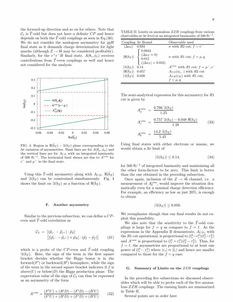
TABLE II: Limits on anomalous ZZH couplings from variousobservables at 3σ level at an integrated luminosity of 500 fb−1.

Coupling 3σ Bound Observable used|∆aZ | 0.034 σ with R2 cut; f = e−

|ℜ(bZ)|

8

>

>

<

>

>

:

0.0044(∆aZ = 0)0.012(|∆aZ | = 0.034)

σ with R1 cut; f = µ, q

|ℑ(bZ)| 0.14 Acom with R1 cut; f = µ−, e−

|ℜ(bZ)| 0.057 AUD(φe−) with R2 cut

|ℑ(bZ)| 0.038 AF B(cH) with R1 cut;f = µ, q

The semi-analytical expression for this asymmetry for R1cut is given by

Acomµ =

0.766 ℑ(bZ)

1.25

Acome =

0.757 ℑ(bZ) − 0.048 ℜ(bZ)

1.28(33)

Acomb =

14.2 ℑ(bZ)

5.45

Using final states with either electrons or muons, wewould obtain a 3σ limit of

|ℑ(bZ)| ≤ 0.14, (34)

for 500 fb−1 of integrated luminosity and maintaining allthe other form-factors to be zero. This limit is betterthan the one obtained in the preceding subsection.

Once again, inclusion of the Z → bb channel, i.e. ameasurement of Acom

b , would improve the situation dra-matically even for a nominal charge detection efficiency.For example, an efficiency as low as just 20%, is enoughto obtain

|ℑ(bZ)| ≤ 0.050.

We reemphasize though that our final results do not ex-ploit this possibility.

We also note that the sensitivity to the T -odd cou-plings is large for f = q as compare to f = ℓ. As theexpressions in the Appendix B demonstrate, AUD, withthe R1 cut operational, is proportional to (l2e−r2

e)(l2f−r2f )

and Acom is proportional to (l2e + r2e)(l2f − r2

f ). Thus, forf = ℓ, the asymmetries are proportional to at least onepower of (l2e − r2

e) where |re| ≈ |le| and hence are smallercompared to those for the f = q case.

G. Summary of Limits on the ZZH couplings

In the preceding five subsections we discussed observ-ables which will be able to probe each of the five anoma-lous ZZH couplings. The ensuing limits are summarizedin Table II.

Several points are in order here

9

• Recall that, of the five anomalous terms, only twoviz ∆aZ and ℜ(bZ), have identical transformations

under both CP and T . Consequently, the contribu-tions proportional to the two are intertwined andcan only be partially separated. In fact, the mostgeneral limits on these two are to be obtained fromFig. 2.

• As for the other three couplings, we have been ableto construct observables that are sensitive to onlya single coupling, thereby disengaging each of thecorresponding bounds in Table II from contamina-tions from any of the other couplings.

• The polar-azimuthal asymmetry, A(θ, φ), is sensi-

tive to T -odd couplings. However, the limits ob-tained using µ final state alone are weaker thanthe ones obtained by combining AR2

UD and Acom

(see Fig 4). Inclusion of electrons in the final statewill improve the sensitivity of A(θ, φ), but only at

the cost of contamination by the T -even ZZH cou-plings. Thus, in our present analysis, the role ofA(θ, φ) is only a confirmatory one.

• Note, however, that many of these asymmetries areproportional to (l2e − r2

e) = (1 − 4 sin2 θW ). Sincethis parameter is known to receive large radiativecorrections, the importance of calculating higher-order effects cannot but be under-emphasized.

• Observables constraining T -odd couplings requiredcharge determination of fermion f in the f fH(bb)final state thereby eliminating (the dominant) f =q final states from the analysis. This explains arelatively poor limit on ℑ(bZ). For f = ν, theprocess involves WWH couplings as well. This isdiscussed in the next section.

IV. THE WWH COUPLINGS

As discussed at the beginning of the last section, thecontribution from non-standard ZZH couplings to theννH(bb) final state is not negligible even if on-shell Zproduction is disallowed by imposing the aforementionedR2 cut. With the neutrinos being invisible, we are leftwith only two observables: the total cross-section and theforward-backward asymmetry with respect to the polarangle of the Higgs boson. The deviation from the SM ex-pectations for the cross section depends mainly on ∆aV

and ℜ(bV ). Similarly, the forward-backward asymme-

try can be parameterized, in the large, by just ℑ(bV ).The contribution of the other couplings, viz. ℑ(bV ) and

ℜ(bV ), to either of these observables are proportional tothe absorptive part of Z-propagator and are understand-ably suppressed, especially for the R2 cut.

Now, irrespective of the CP properties of the Higgs,its decay products are always symmetrically distributedin its rest frame. In addition, the momentum of the in-dividual neutrino is not available for the construction ofany T−odd asymmetry. Consequently, we do not havea direct probe of ℑ(bV ) and ℜ(bV ), i.e. the T−odd cou-plings.

The event selection criteria we use are the same asin previous section except that the cuts of Eqs. (4& 6) are replaced by that of Eq. (8). Imposing∆aW = ∆aZ ≡ ∆a as argued for earlier, the resul-tant cross-section, for the R1′ cut, can be parameterizedas,

σ1 = [7.69 (1 + η1) − 1.89 ℑ(bZ)

+0.458 ℜ(bW ) + 0.786 ℑ(bW )] fb (35)

while the R2′ cut would lead to

σ2 = [52.1 (1 + 2 ∆a) − 6.99 ℜ(bZ)

−0.162ℑ(bZ) − 19.5 ℜ(bW )] fb (36)

Note here that the same η1 = 2 ∆a + 9.46 ℜ(bZ) as de-fined in Eq.(19) appears above owing to the assumption∆aW = ∆aZ ≡ ∆a. As the contributions proportionalto ℑ(bV ) appear due to interference of the WW−fusiondiagram with the absorptive part of the Z-propagatorin Bjorken diagram, formally, these terms are at one or-der of perturbation higher than the rest. Note that thebounds in Table II imply that

|6.99 ℜ(bZ) + 0.162ℑ(bZ)| ≤ 0.0839

and hence the corresponding contribution to σ2 is at theper-mille level. Since we are not sensitive to such smallcontributions, we may safely ignore this combination forall further analysis. Looking at fluctuations in σ2, the 3σbound would, then, be

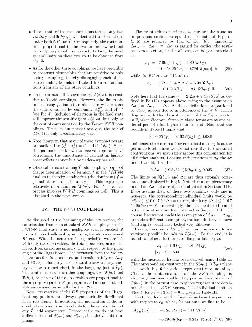
|2 ∆a − (19.5/52.1)ℜ(bW )| ≤ 0.035. (37)

The limits on ℜ(bW ) and ∆a are thus strongly corre-lated and displayed in Fig.5. Note that a complementarybound on ∆a had already been obtained in Section III B.If we assume that, of these two couplings, only one isnon-zero, the corresponding individual limits would be|ℜ(bW )| ≤ 0.097 (if ∆a = 0) and, similarly, |∆a| ≤ 0.017(if ℜ(bW ) = 0). Interestingly, the last mentioned boundis twice as strong as that obtained in Section III B. Ofcourse, had we not made the assumption of ∆aW = ∆aZ ,or made a different assumption, the bounds derived above(and Fig.5) would have looked very different.

Having constrained ℜ(bW ), we may now use σ1 to in-vestigate possible bounds on ℑ(bW ). To this end, it isuseful to define a further subsidiary variable κ1 as

κ1 ≡ 7.69 η1 − 1.89 ℑ(bZ),

|κ1| ≤ 0.604(38)

with the inequality having been derived using Table II.The corresponding constraint in the ℜ(bW )–ℑ(bW ) planeis shown in Fig. 6 for various representative values of κ1.Clearly, the contamination from the ZZH couplings isvery large and inescapable. Any precise measurement ofℑ(bW ), in the present case, requires very accurate deter-mination of the ZZH vertex. The individual limit onℑ(bW ), for κ1 = ℜ(bW ) = 0 is given in Table III.

Next, we look at the forward-backward asymmetrywith respect to cH which, for our cuts, we find to be

A1FB(cH) =

[−1.20 ℜ(bZ) − 7.11 ℑ(bZ)

+0.294 ℜ(bW ) − 0.242 ℑ(bW )]/7.69 (39)

10

-0.3

-0.2

-0.1

0

0.1

0.2

0.3

-0.04 -0.02 0 0.02 0.04

Re(

b W)

∆a (=∆aZ=∆aW)

σ(R2; e)σR2

FIG. 5: Region of ∆a − ℜ(bW ) plane corresponding to 3σvariation of σ2 for L = 500 fb−1. The vertical line shows thelimit on ∆aZ from Fig. 2.

-1.5

-1

-0.5

0

0.5

1

1.5

-0.1 -0.05 0 0.05 0.1

Im(b

W)

Re(bW)

κ1 = -0.6

κ1 = 0.6

κ1 = 0.0

FIG. 6: Region of ℑ(bW )−ℜ(bW ) plane corresponding to 3σvariation of σ1 for κ1=0.0 (big-dashed line), 0.6 (solid line)and −0.6 (small-dashed line). Vertical lines show limit onℜ(bW ) obtained from Fig. 5 for ∆a = 0.

for the R1′ cut, while for the R2′ cut it is

A2FB(cH) =

[3.55 ℑ(bZ) + 4.00 ℑ(bW )

]/52.1 (40)

Clearly A2FB is the one that is more sensitive to ℑ(bW ).

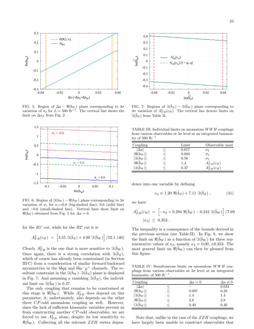
Once again, there is a strong correlation with ℑ(bZ),which of course has already been constrained (in SectionIII C) from a consideration of similar forward-backwardasymmetries in the bbqq and bbµ−µ+ channels. The re-sultant constraint in the ℑ(bW )–ℑ(bZ) plane is displayed

in Fig. 7. And assuming a vanishing ℑ(bZ), the individ-

ual limit on ℑ(bW ) is 0.37.The only coupling that remains to be constrained at

this stage is ℜ(bW ). While A1FB does depend on this

parameter, it, unfortunately, also depends on the otherthree CP -odd anomalous coupling as well. However,since the lack of sufficient kinematic variables prevent usfrom constructing another CP -odd observables, we areforced to use A1

FB alone, despite its low sensitivity to

ℜ(bW ). Collecting all the relevant ZZH vertex depen-

-0.4

-0.3

-0.2

-0.1

0

0.1

0.2

0.3

0.4

-0.04 -0.02 0 0.02 0.04

Im(∼ b W

)

Im(∼bZ)

A2FB(cH)

AFB(cH) [f = µ, q]

FIG. 7: Regions of ℑ(bZ) − ℑ(bW ) plane corresponding to3σ variation of A2

F B(cH). The vertical line denote limits on

ℑ(bZ) from Table II.

TABLE III: Individual limits on anomalous WWH couplingsfrom various observables at 3σ level at an integrated luminos-ity of 500 fb−1

Coupling Limit Observable used|∆a| ≤ 0.017 σ2

|ℜ(bW )| ≤ 0.094 σ2

|ℑ(bW )| ≤ 0.56 σ1

|ℜ(bW )| ≤ 1.4 A1F B(cH)

|ℑ(bW )| ≤ 0.37 A2F B(cH)

dence into one variable by defining

κ3 ≡ 1.20 ℜ(bZ) + 7.11 ℑ(bZ) , (41)

we have

A1FB(cH) =

[−κ3 + 0.294 ℜ(bW ) − 0.242 ℑ(bW )

]/7.69

|κ3| ≤ 0.353 .

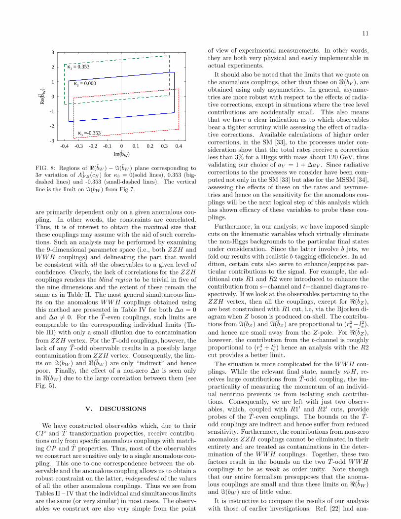
The inequality is a consequence of the bounds derived inthe previous section (see Table.II). In Fig. 8, we show

the limit on ℜ(bW ) as a function of ℑ(bW ) for three rep-resentative values of κ3, namely κ3 = 0.00,±0.353. Themost general limit on ℜ(bW ) can then be gleaned fromthis figure.

TABLE IV: Simultaneous limits on anomalous WWH cou-plings from various observables at 3σ level at an integratedluminosity of 500 fb−1.

Coupling ∆a = 0 ∆a 6= 0|∆a| ≤ – 0.034

|ℜ(bW )| ≤ 0.097 0.28|ℑ(bW )| ≤ 1.4 1.4

|ℜ(bW )| ≤ 2.8 2.8

|ℑ(bW )| ≤ 0.40 0.40

Note that, unlike in the case of the ZZH couplings, wehave largely been unable to construct observables that

11

-3

-2

-1

0

1

2

3

-0.4 -0.3 -0.2 -0.1 0 0.1 0.2 0.3 0.4

Re(

∼ b W)

Im(∼bW)

κ3 = 0.353

κ3 = 0.000

κ3 =-0.353

FIG. 8: Regions of ℜ(bW ) − ℑ(bW ) plane corresponding to3σ variation of A1

F B(cH) for κ3 = 0(solid lines), 0.353 (big-dashed lines) and -0.353 (small-dashed lines). The vertical

line is the limit on ℑ(bW ) from Fig 7.

are primarily dependent only on a given anomalous cou-pling. In other words, the constraints are correlated.Thus, it is of interest to obtain the maximal size thatthese couplings may assume with the aid of such correla-tions. Such an analysis may be performed by examiningthe 9-dimensional parameter space (i.e., both ZZH andWWH couplings) and delineating the part that wouldbe consistent with all the observables to a given level ofconfidence. Clearly, the lack of correlations for the ZZHcouplings renders the blind region to be trivial in five ofthe nine dimensions and the extent of these remain thesame as in Table II. The most general simultaneous lim-its on the anomalous WWH couplings obtained usingthis method are presented in Table IV for both ∆a = 0and ∆a 6= 0. For the T -even couplings, such limits arecomparable to the corresponding individual limits (Ta-ble III) with only a small dilution due to contamination

from ZZH vertex. For the T -odd couplings, however, thelack of any T -odd observable results in a possibly largecontamination from ZZH vertex. Consequently, the lim-its on ℑ(bW ) and ℜ(bW ) are only “indirect” and hencepoor. Finally, the effect of a non-zero ∆a is seen onlyin ℜ(bW ) due to the large correlation between them (seeFig. 5).

V. DISCUSSIONS

We have constructed observables which, due to theirCP and T transformation properties, receive contribu-tions only from specific anomalous couplings with match-ing CP and T properties. Thus, most of the observableswe construct are sensitive only to a single anomalous cou-pling. This one-to-one correspondence between the ob-servable and the anomalous coupling allows us to obtain arobust constraint on the latter, independent of the valuesof all the other anomalous couplings. Thus we see fromTables II – IV that the individual and simultaneous limitsare the same (or very similar) in most cases. The observ-ables we construct are also very simple from the point

of view of experimental measurements. In other words,they are both very physical and easily implementable inactual experiments.

It should also be noted that the limits that we quote onthe anomalous couplings, other than those on ℜ(bV ), areobtained using only asymmetries. In general, asymme-tries are more robust with respect to the effects of radia-tive corrections, except in situations where the tree levelcontributions are accidentally small. This also meansthat we have a clear indication as to which observablesbear a tighter scrutiny while assessing the effect of radia-tive corrections. Available calculations of higher ordercorrections, in the SM [33], to the processes under con-sideration show that the total rates receive a correctionless than 3% for a Higgs with mass about 120 GeV, thusvalidating our choice of aV = 1 + ∆aV . Since radiativecorrections to the processes we consider have been com-puted not only in the SM [33] but also for the MSSM [34],assessing the effects of these on the rates and asymme-tries and hence on the sensitivity for the anomalous cou-plings will be the next logical step of this analysis whichhas shown efficacy of these variables to probe these cou-plings.

Furthermore, in our analysis, we have imposed simplecuts on the kinematic variables which virtually eliminatethe non-Higgs backgrounds to the particular final statesunder consideration. Since the latter involve b jets, wefold our results with realistic b-tagging efficiencies. In ad-dition, certain cuts also serve to enhance/suppress par-ticular contributions to the signal. For example, the ad-ditional cuts R1 and R2 were introduced to enhance thecontribution from s−channel and t−channel diagrams re-spectively. If we look at the observables pertaining to theZZH vertex, then all the couplings, except for ℜ(bZ),are best constrained with R1 cut, i.e, via the Bjorken di-agram when Z boson is produced on-shell. The contribu-tions from ℑ(bZ) and ℑ(bZ) are proportional to (r2

e − l2e),

and hence are small away from the Z-pole. For ℜ(bZ),however, the contribution from the t-channel is roughlyproportional to (r4

e + l4e) hence an analysis with the R2cut provides a better limit.

The situation is more complicated for the WWH cou-plings. While the relevant final state, namely ννH , re-ceives large contributions from T -odd coupling, the im-practicality of measuring the momentum of an individ-ual neutrino prevents us from isolating such contribu-tions. Consequently, we are left with just two observ-ables, which, coupled with R1′ and R2′ cuts, provideprobes of the T -even couplings. The bounds on the T -odd couplings are indirect and hence suffer from reducedsensitivity. Furthermore, the contributions from non-zeroanomalous ZZH couplings cannot be eliminated in theirentirety and are treated as contaminations in the deter-mination of the WWH couplings. Together, these twofactors result in the bounds on the two T -odd WWHcouplings to be as weak as order unity. Note thoughthat our entire formalism presupposes that the anoma-lous couplings are small and thus these limits on ℜ(bW )and ℑ(bW ) are of little value.

It is instructive to compare the results of our analysiswith those of earlier investigations. Ref. [22] had ana-

12

lyzed the case of ZZH couplings with (out) initial beampolarization. We find that the effect of realistic cuts onkinematic variables required to isolate the signal with thedominant final state with bb as well as the finite b-taggingefficiency, reduces the possible limits on bZ by about afactor of 2, compared to the ones quoted in Ref. [22] withunpolarized beams. Needless to say, if the reduction inrates implied by these cuts is neglected, our analysis doesreproduce the results of Ref. [22].

In Ref. [20], an optimal observable analysis [21] is per-formed, including along with an additional anomalousZγH coupling. While such optimal variable analysesgenerally indicate the maximum achievable sensitivity,the observables constructed very often remain a littleopaque with respect to the physics they probe. The pa-rameterization of Ref. [20] is quite different from ours.Still, making use of the correlation matrices given bythem, and putting the ZγH coupling to zero, one mayextract the limits their analysis will imply for our pa-rameterization. Doing this, we find that, for the T -evencouplings, our limits compare quite well with those ob-tained in the analysis of Ref. [22], implying thereby that

our simple T observables indeed catch the physics con-tent of their optimal observables in this case. For theT -odd couplings, our use of simple observable like theexpectation value of sign of C1,2 rather than the expec-tation value of the momentum correlator, 〈C1,2〉 causesa loss in sensitivity only by a factor 4. Given the factthat some of this is attributable to our use of realistickinematic cuts, b-tagging efficiencies etc, this is a verymodest price to pay for the simplicity of the observable.The optimal observable analysis shows that the use ofZ → bb and Z → τ+τ− final states and polarization ofthe beams can improve the sensitivity significantly. Thisis a very good motivation for constructing analogous sim-ple observables similar to the ones constructed here.

To summarize, we have looked at the Higgs productionprocesses at an e+e− collider involving V V H coupling.We constructed several observables with appropriate CPand T properties to probe various anomalous couplingsincorporating realistic cuts and detection efficiencies.

Using these observables in the context of ZZ fusionand Higgstrahlung processes, we obtain stringent but re-alistic bounds on the various anomalous ZZH couplings,even while allowing for maximal cancellations betweenthe various individual contributions. As for the WWHcouplings, their effects cannot be fully isolated from thoseof the ZZH couplings. Nonetheless, we are able to derivequite stringent bounds for the T -even subset even whileaccounting for maximal contamination from theZZHsector. On the other hand, the lack of suitable T -oddobservables render the limits on the T -odd WWH cou-plings to be only indirect and thus poor. We reemphasizethat all our asymmetries are simple to construct, havespecific CP and T properties to probe specific anoma-lous coupling, and are robust against both the radiativecorrection to the rates as well as systematic errors.

Acknowledgments

We thank B. Mukhopadhyaya for collaboration in theinitial phase of this project and S. D. Rindani, M. Schu-macher and K. Moenig for useful discussions and S.K. Rai for reading the manuscript. We would like toacknowledge support from the Department of Scienceand Technology under project number SR/FIST/PSI-022/200, to the Center for High Energy Physics, IISc,for the cluster which was used for computations. Thework was also partially supported under the DSTproject SP/S2/K-01/2000-II and the Indo-French projectIFC/3004-B/2004. RKS wishes to thank Harish-ChandraResearch Institute for hospitality where this work wasstarted and Council for Scientific and Industrial Researchfor the financial support. DC thanks the DST, India forfinancial assistance under the Swarnajayanti grant.

APPENDIX A: PARTIAL CROSS-SECTIONS

AND ANOMALOUS COUPLINGS

As mentioned in Section IIB, the total cross-sectionfor e+e− → f fH receives contributions only from CP -even and T -even couplings ∆aV and ℜ(bV ), while theother couplings contribute to partial cross-section in sucha way that their net contribution to the total rate iszero. In our analysis so far, we considered appropriatelychosen partial cross-sections and combined them to con-struct asymmetries. In its stead, we could, in principle,have considered just the partial cross sections themselvesand investigated their resolving power. This, we attemptnow.

To start with, we look at e+e− → µ−µ+H and con-strain the Higgs boson to be in the forward direction(cos θe−H > 0) and µ− to be above the Higgs produc-tion plane (sinφµ > 0). This partial cross-section, called“forward-up” and denoted by (F ′U) in section III F, isplotted as a function of Ecm in Fig. 9 for the SM. Alsoshown are the corresponding cross-sections when only oneanomalous coupling is non-zero. The large values of theanomalous couplings have been chosen to highlight thedifferences.

We see that all four anomalous couplings contributeto the (F ′U) partial cross-section, which can now beparametrized as

σF ′U = σ0 + ℜ(bZ)σ1 + ℑ(bZ)σ2 + ℜ(bZ)σ3 + ℑ(bZ)σ4.(A1)

If only one anomalous coupling Bi were to be non-zero,then the measurement of this partial cross-section wouldbe sensitive to

|Bi| ≥d

|σi|

√σ0

L + ǫ2(σ0)2. (A2)

Here d is the degree of statistical significance, L is theintegrated luminosity of the e+e− collider and ǫ is thefractional systematic error. In Fig. 10, we show a simple(d = 1, ǫ = 0.01) limit on anomalous couplings, obtainedusing Fig. 9, for an integrated luminosity of 500 fb−1. Ameasurement of σF ′U will thus be sensitive to values ofBi lying above the corresponding curve.

13

-0.5

0

0.5

1

1.5

2

2.5

3

3.5

4

200 300 400 500 600 700 800 900 1000

σ(µ+ µ− H

) [f

b]

Ecm [GeV]

H : forward; cosθ > 0µ−: upward; sinφµ > 0

SMSM+Re(bz)=0.1SM+Im(bz)=1.0

SM+Re(~bz)=1.0

SM+Im(~bz)=1.0

FIG. 9: Partial cross-sections as a function of c.m. energy forthe process e+e− → µ+µ−H with Higgs boson in the forwarddirection and the final state µ− above the Higgs boson’s pro-duction plane. A Higgs boson of mass 120 GeV is assumed.

0

0.05

0.1

0.15

0.2

0.25

0.3

200 300 400 500 600 700 800 900 1000

b lim

Ecm [GeV]

Re(bz)Im(bz)Re(~bz)Im(~bz)

FIG. 10: Limits on various non-standard coupling obtainedusing Eq.(A2) with d = 1 and ǫ = 0.01 for an integrated lu-minosity of 500 fb−1 and using cross-sections shown in Fig. 9.

A similar exercise can be done for e+e− → e+e−H , andin Fig. 11(a) we display the (F ′U) partial cross-section forthe same as a function of the center-of-mass energy. Thepresence of an additional t-channel diagram changes theEcm behaviour of the partial cross-section and hence thatof the limits that could be inferred in a fashion analogousto Fig. 9.

For ℜ(bZ) and ℑ(bZ), the 3σ bounds of Table II aremuch better than the 1σ limits shown in Fig. 10. Thisindicates that asymmetries with appropriate symmetryproperties and combinations of various final states can beused efficiently to obtain stringent constraints on anoma-lous couplings.

For ℑ(bZ), on the other hand, the limit obtained usingAcom

µ is only comparable to the one obtained using justthe partial rate σ(F ′U) after accounting for degrees ofsignificance. However, the limit from σ(F ′U) is subjectto the assumption that all other anomalous couplings arezero, while the one obtained using Acom

µ is independentof any other anomalous coupling. Once again this un-derscores the importance of specific observables, such as

Acom, which receive a contribution from only one of theanomalous coupling, thus allowing us to obtain a robustconstraint.

And finally, we look at the e+e− → νeνeH channel,where both WWH and ZZH vertices contribute thusdoubling the number of anomalous couplings involved.Since the final state fermions, the neutrinos, are not de-tectable, it is meaningless to construct the partial cross-section (F ′U). Instead we add (F ′U) and (F ′D) toform the “forward” cross-section, i.e. the Higgs bosonis constrained to be in the forward direction, and theEcm dependence is displayed in Fig. 11(b). The size ofthe anomalous contribution in these figures gives an ideaabout the sensitivity to that particular coupling.

0

1

2

3

4

5

6

7

200 300 400 500 600 700 800 900 1000

σ(e

+e- H

) [f

b]

Ecm [Gev]

H : forward; cosθH > 0e−: upward; sinφe > 0

(a)SMSM+Re(bz)=0.1SM+Im(bz)=1.0

SM+Re(~bz)= 0.1

SM+Im(~bz)= 1.0

0

20

40

60

80

100

120

140

160

180

200

200 300 400 500 600 700 800 900 1000

σ(ν

− νH)

[fb]

Ecm[Gev]

H : forward; cosθH > 0

(b) SMSM+Re(bz)=1.0SM+Im(

~bz)=1.0

SM+Re(bw)=1.0SM+Im(

~bw)=1.0

FIG. 11: Cross-sections as functions of the c.m. energyfor a Higgs boson of mass 120 GeV and particular valuesfor the anomalous couplings. (a) Partial cross-sections fore+e− → e+e−H with forward Higgs boson and the final statee− above the Higgs boson’s production plane. (b) Partialcross-sections for e+e− → ννH with the Higgs boson in theforward direction.

APPENDIX B: EXPRESSIONS FOR |M2|

In this appendix, we list the square of invariant matrixelement for the various processes considered in the text.

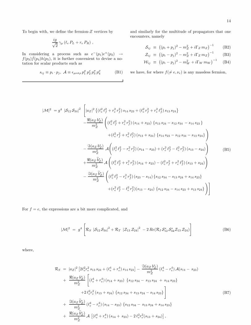
14

To begin with, we define the fermion-Z vertices by

ig√2

γµ (ℓe PL + re PR) ,

In considering a process such as e−(p1)e+(p2) →

f(p3)f(p4)h(p5), it is further convenient to devise a no-tation for scalar products such as

sij ≡ pi · pj , A ≡ ǫµνσρ pµ1 pν

2 pσ3 pρ

4 (B1)

and similarly for the multitude of propagators that oneencounters, namely

Sij ≡((pi + pj)

2 − m2Z + iΓZ mZ

)−1(B2)

Zij ≡((pi − pj)

2 − m2Z + iΓZ mZ

)−1(B3)

Wij ≡((pi − pj)

2 − m2W + iΓW mW

)−1(B4)

we have, for where f(6= e, νe) is any massless fermion,

|M|2 = g4 |S12 S34|2[|aZ |2

{(ℓ2

e ℓ2f + r2

e r2f ) s14 s23 + (ℓ2

e r2f + r2

e ℓ2f ) s13 s24

}

−ℜ(aZ b∗Z)

m2Z

((ℓ2

e ℓ2f + r2

e r2f ) (s14 + s23) {s13 s24 − s12 s34 − s14 s23 }

+(ℓ2e r2

f + r2e ℓ2

f ) (s13 + s24) {s14 s23 − s12 s34 − s13 s24})

− ℑ(aZ b∗Z)

m2Z

A(

(ℓ2e ℓ2

f − r2e r2

f ) (s14 − s23) + (r2e ℓ2

f − ℓ2e r2

f ) (s13 − s24)

)

+ℜ(aZ b∗Z)

m2Z

A(

(ℓ2e ℓ2

f + r2e r2

f ) (s14 + s23) − (ℓ2e r2

f + r2e ℓ2

f ) (s13 + s24)

)

− ℑ(aZ b∗Z)

m2Z

((ℓ2

e ℓ2f − r2

e r2f ) (s23 − s14) {s12 s34 − s13 s24 + s14 s23}

+(r2e ℓ2

f − ℓ2e r2

f )(s13 − s24) {s12 s34 − s14 s23 + s13 s24})]

(B5)

For f = e, the expressions are a bit more complicated, and

|M|2 = g4

[RS |S12 S34|2 + RT |Z13 Z24|2 − 2 Re(RI S∗

12 S∗34Z13 Z24)

](B6)

where,

RS = |aZ |2[2ℓ2

er2e s13 s24 + (ℓ4

e + r4e) s14 s23

]− ℑ(aZ b∗Z)

m2Z

(ℓ4e − r4

e)A(s14 − s23)

+ℜ(aZ b∗Z)

m2Z

[(ℓ4

e + r4e) (s14 + s23) {s12 s34 − s13 s24 + s14 s23}

+2 ℓ2er

2e (s13 + s24) {s12 s34 + s13 s24 − s14 s23}

]

+ℑ(aZ b∗Z)

m2Z

(ℓ4e − r4

e) (s14 − s23) {s12 s34 − s13 s24 + s14 s23}

+ℜ(aZ b∗Z)

m2Z

A[(ℓ4

e + r4e) (s14 + s23) − 2 ℓ2

er2e(s13 + s24)

],

(B7)

15

RT = |aZ |2[(ℓ4

e + r4e) s14 s23 + 2 ℓ2

e r2e s12 s34

]− ℑ(aZ b∗Z)

m2Z

(r4e − ℓ4

e)A (s14 − s23)

+ℜ(aZ b∗Z)

m2Z

[(ℓ4

e + r4e) (s14 + s23) {− s12 s34 + s13 s24 + s14 s23}

+2 ℓ2er

2e (s12 + s34) {−s13 s24 − s12 s34 + s14 s23}

]

+ℑ(aZ b∗Z)

m2Z

(r4e − ℓ4

e) (s23 − s14) {−s12 s34 + s13 s24 + s14 s23 }

− ℜ(aZ b∗Z)

m2Z

A[(ℓ4

e + r4e)(s14 + s23) + 2 ℓ2

e r2e (s12 + s34)

],

RI = −|aZ |2 (ℓ4e + r4

e) s14 s23

+(ℓ4

e − r4e)

m2Z

(s23 − s14)[iℜ(aZ b∗Z) A + iℜ(aZ b∗Z) (s13 s24 − s12 s34) + ℑ(aZ b∗Z) s14 s23

]

− (ℓ4e + r4

e)

m2Z

(s14 + s23)[iℑ(aZ b∗Z) (s12 s34 − s13 s24) + iℑ(aZ b∗Z)A + ℜ(aZ b∗Z) s14 s23

](B8)

And finally, for f = νe,

|M|2 = g4

[ℓ2νRS |S12 S34|2 + RT |W13 W24|2 − ℓν ℓeℜ(RI S∗

12 S∗34W13 W24)

](B9)

where,

RS = |aZ |2[ℓ2e s14 s23 + r2

e s13 s24

]+

ℑ(aZ b∗Z)

m2Z

A[ℓ2e (s23 − s14) + r2

e (s24 − s13)

]

+ℜ(aZ b∗Z)

m2Z

[ℓ2e (s14 + s23) {s12 s34 − s13 s24 + s14 s23} + r2

e (s13 + s24) {s12 s34 + s13 s24 − s14 s23}]

+ℑ(aZ b∗Z)

m2Z

[ℓ2e (s14 − s23) {s12 s34 − s13 s24 + s14 s23} + r2

e (s24 − s13) {s12 s34 + s13 s24 − s14 s23}]

− ℜ(aZ b∗Z)

m2Z

A[r2e (s13 + s24) − ℓ2

e (s14 + s23)

], (B10)

RT = |aW |2 s14 s23 +ℜ(aW b∗W )

m2W

(s14 + s23) {− s12 s34 + s13 s24 + s14 s23} +ℑ(aW b∗W )

m2W

A (s14 − s23)

+ℑ(aW b∗W )

m2W

(s14 − s23) {− s12 s34 + s13 s24 + s14 s23} −ℜ(aW b∗W )

m2W

A (s14 + s23) (B11)

RI = −2 aW a∗Z s14 s23 −

aW b∗Zm2

Z

[(s14 + s23) {s12 s34 − s13 s24 + s14s23} + i A (s14 − s23)

]

− iaW b∗Zm2

Z

[(s23 − s14) {s12 s34 − s13 s24 + s14 s23} − i A (s14 + s23)

]

+a∗

Z bW

m2W

[(s14 + s23) {s12 s34 − s13 s24 − s14 s23} − i A (s14 − s23)

]

+ ia∗

Z bW

m2W

[(s23 − s14) {−s12 s34 + s13 s24 + s14 s23} − i A (s14 + s23)

](B12)

In the propagators, we ignore the contribution proportional to ΓV except for S34, which goes on-shell, and cannot beignored, in general.

16

[1] For a review, see for example, R. M. Godbole,[arXiv:hep-ph/0205114], Volume 4, Jubilee Issue of theIndian Journal of Physics, pp. 44-83, 2004, Guest Edi-tors: A. Raychaudhuri and P. Mitra.

[2] ALEPH, DELPHI, L3 and OPAL Collaborations, TheLEP Working Group for Higgs Boson Searches, Phys.Lett. B 565, 61 (2003);see also http://lephiggs.web.cern.ch/LEPHIGGS/

[3] LEP Electroweak Working Group,http://lepewwg.web.cern.ch/LEPEWWG/

[4] R. Akers et al. [OPAL Collaboration], Z. Phys. C 61,19 (1994); D. Buskulic et al. [ALEPH Collaboration], Z.Phys. C 62, 539 (1994); M. Acciarri et al. [L3 Collabora-tion], Z. Phys. C 62, 551 (1994); P. Abreu et al. [DELPHICollaboration], Z. Phys. C 67, 69 (1995); D. Antreasyanet al. [Crystal Ball Collaboration], Phys. Lett. B 251,204 (1990); P. Franzini et al., Phys. Rev. D 35, 2883(1987); J. Kalinowski and M. Krawczyk, Phys. Lett.B 361, 66 (1995) [arXiv:hep-ph/9506291]; D. Choud-hury and M. Krawczyk, Phys. Rev. D 55, 2774 (1997)[arXiv:hep-ph/9607271].

[5] M. Carena, J. R. Ellis, A. Pilaftsis and C. E. M. Wagner,Nucl. Phys. B586, 92 (2000); A. Mendez and A. Po-marol, Phys. Lett. B 279, 98 (1992); J. F. Gunion,H. E. Haber and J. Wudka, Phys. Rev. D 43, 904(1991); J. F. Gunion, B. Grzadkowski, H. E. Haberand J. Kalinowski, Phys. Rev. Lett. 79, 982 (1997)[hep-ph/9704410]; I. F. Ginzburg, M. Krawczyk andP. Osland, hep-ph/0211371.

[6] G. Abbiendi et al. [OPAL Collaboration], Eur. Phys. J.

C 37, 49 (2004); ALEPH, DELPHI, L3 and OPAL Col-laborations, The LEP Working Group for Higgs BosonSearches, LHWG-Note 2004-01.

[7] See for example, J. R. Forshaw, Pramana 63, 1119(2004) and discussion therein; see also D. Choudhury,T. M. P. Tait and C. E. M. Wagner, Phys. Rev. D 65,053002 (2002) [arXiv:hep-ph/0109097].

[8] ATLAS Collaboration, Detector and Physics Perfor-

mance Technical Design Report, CERN-LHCC-99-14 &15 (1999); CMS Collaboration, Technical Design Report,CERN-LHCC-97-10 (1997).

[9] See for example, M. Drees, R. M. Godbole, P. Roy, The-

ory and Phenomenology of Sparticles , World Scientific,2004.

[10] For a brief review, see for example, R. M. Godbole,S. Kraml, M. Krawczyk, D. J. Miller, P. Niezurawskiand A. F. Zarnecki, arXiv:hep-ph/0404024 and referencestherein.

[11] R. L. Kelly and T. Shimada, Phys. Rev. D 23,1940 (1981); P. Kalyniak, J. N. Ng, P. Zakarauskas,Phys. Rev. D 29, 502 (1984). W. Kilian, M. Kramerand P. M. Zerwas, Phys. Lett. B 373, 135 (1996)[arXiv:hep-ph/9512355].

[12] J. C. Romao and A. Barroso, Phys. Lett. B 185, 195(1987).

[13] R. Rattazzi, Z. Phys. C 40, 605 (1988).[14] K. Hagiwara and M. L. Stong, Z. Phys. C 62, 99 (1994).[15] H. J. He, Y. P. Kuang, C. P. Yuan and B. Zhang, Phys.

Lett. B 554, 64 (2003) [arXiv:hep-ph/0211229].

[16] K. Hagiwara, S. Ishihara, R. Szalapski and D. Zeppen-feld, Phys. Rev. D 48, 2182 (1993); K. Hagiwara, R. Sza-lapski and D. Zeppenfeld, Phys. Lett. B 318, 155 (1993)[arXiv:hep-ph/9308347].

[17] G. J. Gounaris, F. M. Renard and N. D. Vlachos, Nucl.Phys. B 459, 51 (1996) [arXiv:hep-ph/9509316].

[18] B. Zhang, Y. P. Kuang, H. J. He and C. P. Yuan, Phys.Rev. D 67, 114024 (2003) [arXiv:hep-ph/0303048].

[19] T. Plehn, D. Rainwater and D. Zeppenfeld, Phys. Rev.Lett. 88 051801 (2002)

[20] K. Hagiwara, S. Ishihara, J. Kamoshita and B. A. Kniehl,Eur. Phys. J. C 14, 457 (2000) [arXiv:hep-ph/0002043].

[21] D. Atwood and A. Soni, Phys. Rev. D 45, 2405 (1992).[22] T. Han and J. Jiang, Phys. Rev. D 63, 096007 (2001)[23] P. Niezurawski, A. F. Zarnecki and M. Krawczyk, Acta

Phys. Polon. B 36, 833 (2005) [arXiv:hep-ph/0410291].[24] B. A. Kniehl, Nucl. Phys. B 352, 1 (1991); Nucl. Phys.

B 357, 439 (1991)[25] M. C. Gonzalez-Garcia, Int. J. Mod. Phys. A 14,

3121 (1999) [arXiv:hep-ph/9902321]. V. Barger, T. Han,P. Langacker, B. McElrath and P. Zerwas, Phys. Rev. D67, 115001 (2003) [arXiv:hep-ph/0301097].

[26] A. Mendez and A. Pomarol, Phys. Lett. B 272, 313(1991).

[27] D. Choudhury, A. Datta and K. Huitu, Nucl. Phys. B673, 385 (2003) [arXiv:hep-ph/0302141].

[28] A. Pilaftsis and C. E. M. Wagner, Nucl. Phys. B 553,3 (1999); M. Carena, H. E. Haber, H. E. Logan andS. Mrenna, Phys. Rev. D 65, 055005 (2002)

[29] V. D. Barger, K.-m. Cheung, A. Djouadi, B. A. Kniehland P. M. Zerwas, Phys. Rev. D 49, 79 (1994)[arXiv:hep-ph/9306270].

[30] D. Choudhury, T. M. P. Tait and C. E. M. Wagner, Phys.Rev. D 65, 115007 (2002) [arXiv:hep-ph/0202162].

[31] For a recent review, see A. Djouadi,arXiv:hep-ph/0503172.

[32] M. Acciarri et al. [L3 Collaboration], Phys. Lett. B 439,225 (1998); P. Abreu et al. [DELPHI Collaboration], Eur.Phys. J. C 9, 367 (1999); S. M. Xella-Hansen, M. Wing,D. J. Jackson, N. De Groot and C. J. S. Damerell, LC-PHSM-2003-061;

[33] A. Denner, S. Dittmaier, M. Roth and M. M. Weber,Nucl. Phys. B 660, 289 (2003) [arXiv:hep-ph/0302198];A. Denner, S. Dittmaier, M. Roth and M. M. We-ber, Nucl. Phys. Proc. Suppl. 135, 88 (2004)[arXiv:hep-ph/0406335]; F. Boudjema et al., Phys.Lett. B 600, 65 (2004) [arXiv:hep-ph/0407065]; G. Be-langer et al, Phys. Lett. B 559, 252 (2003)[arXiv:hep-ph/0212261]; Nucl. Phys. Proc. Suppl. 116,353 (2003) [arXiv:hep-ph/0211268].

[34] T. Hahn, S. Heinemeyer and G. Weiglein, Nucl. Phys. B652, 229 (2003) [arXiv:hep-ph/0211204]; S. Heinemeyerand G. Weiglein, Nucl. Phys. Proc. Suppl. 89, 210 (2000);H. Eberl, W. Majerotto and V. C. Spanos, Nucl. Phys.B 657, 378 (2003) [arXiv:hep-ph/0210038].

[35] Remember that we work only to the linear order in theanomalous couplings. Thus they contribute only throughthe interference terms with the SM amplitude.

http://arXiv.org/abs/hep-ph/0205114

http://lephiggs.web.cern.ch/LEPHIGGS/

http://lepewwg.web.cern.ch/LEPEWWG/



























Signatures of anomalous VVH interactions at a linear collider

Documents

Transcript of Signatures of anomalous VVH interactions at a linear collider