This content has been downloaded from IOPscience. Please scroll down to see the full text.

Download details:

IP Address: 95.46.73.203

This content was downloaded on 15/12/2013 at 13:18

Please note that terms and conditions apply.

The ATLAS Experiment at the CERN Large Hadron Collider

View the table of contents for this issue, or go to the journal homepage for more

2008 JINST 3 S08003

(http://iopscience.iop.org/1748-0221/3/08/S08003)

Home Search Collections Journals About Contact us My IOPscience

2008 JINST 3 S08003

PUBLISHED BY INSTITUTE OF PHYSICS PUBLISHING AND SISSA

RECEIVED: January 8, 2008REVISED: May 6, 2008

ACCEPTED: May 7, 2008PUBLISHED: August 14, 2008

THE CERN LARGE HADRON COLLIDER: ACCELERATOR AND EXPERIMENTS

The ATLAS Experiment at the CERN Large HadronCollider

ATLAS Collaboration

ABSTRACT: The ATLAS detector as installed in its experimental cavern at point 1 at CERN isdescribed in this paper. A brief overview of the expected performance of the detector when theLarge Hadron Collider begins operation is also presented.

KEYWORDS: ATLAS; LHC; CERN; Accelerator; Proton-proton collisions; Heavy-ion collisions;Minimum-bias events; Bunch-crossings; Pile-up; Superconducting magnets; Solenoidal field;Toroidal field; Magnetic field measurements; Hall probes; Inner detector; Charged-particletracking; Vertex measurement; Pixel detectors; Silicon micro-strip detectors; Transition radiation;Time-over-threshold; Radiation-hard electronics; Fluorinert cooling; Carbon-fibre reinforcedplastics; Optical fibres; Calorimetry; Sampling calorimeters; Liquid argon; Scintillator tiles;Electromagnetic and hadronic interactions; Forward calorimetry; Accordion geometry; Lateralsegmentation; Longitudinal segmentation; Muon spectrometer; Precision-tracking chambers;Trigger chambers; Drift tubes; Thin-gap chambers; Resistive-plate chambers; Optical alignmentsystems; Forward detectors; Cerenkov light; Roman Pots; Zero-degree calorimetry; Trigger anddata acquisition; High-level trigger; Event filter; Detector control system; Bandwidth; Processorfarm; Electrons; Muons; Leptons; Photons; Jets; Taus; Missing transverse energy; b-tagging;Particle identification; Tracking algorithms; Vertexing algorithms; Impact parametermeasurements.

c© 2008 IOP Publishing Ltd and SISSA http://www.iop.org/EJ/jinst/

2008 JINST 3 S08003

The ATLAS Collaboration

G. Aad,81 E. Abat,18,∗ J. Abdallah,162 A.A. Abdelalim,46 A. Abdesselam,116 O. Abdinov,10

B.A. Abi,111 M. Abolins,86 H. Abramowicz,150 E. Acerbi,87 B.S. Acharya,159 R. Achenbach,55

M. Ackers,20 D.L. Adams,23 F. Adamyan,169 T.N. Addy,53 M. Aderholz,98 C. Adorisio,35

P. Adragna,72 M. Aharrouche,78 S.P. Ahlen,21 F. Ahles,45 A. Ahmad,146 H. Ahmed,2

G. Aielli,133 P.F. Åkesson,28 T.P.A. Åkesson,76 A.V. Akimov,93 S.M. Alam,1 J. Albert,164

S. Albrand,52 M. Aleksa,28 I.N. Aleksandrov,62 M. Aleppo,87 F. Alessandria,87 C. Alexa,24

G. Alexander,150 T. Alexopoulos,9 G. Alimonti,87 M. Aliyev,10 P.P. Allport,70

S.E. Allwood-Spiers,50 A. Aloisio,101 J. Alonso,14 R. Alves,122 M.G. Alviggi,101 K. Amako,63

P. Amaral,28 S.P. Amaral,28 G. Ambrosini,16 G. Ambrosio,87 C. Amelung,28

V.V. Ammosov,126 A. Amorim,122 N. Amram,150 C. Anastopoulos,151 B. Anderson,74

K.J. Anderson,29 E.C. Anderssen,14 A. Andreazza,87 V. Andrei,55 L. Andricek,98

M-L. Andrieux,52 X.S. Anduaga,67 F. Anghinolfi,28 A. Antonaki,8 M. Antonelli,44

S. Antonelli,19 R. Apsimon,127 G. Arabidze,8 I. Aracena,142 Y. Arai,63 A.T.H. Arce,14

J.P. Archambault,27 J-F. Arguin,14 E. Arik,18,∗ M. Arik,18 K.E. Arms,108 S.R. Armstrong,23

M. Arnaud,135 C. Arnault,113 A. Artamonov,94 S. Asai,152 S. Ask,79 B. Åsman,144 D. Asner,27

L. Asquith,74 K. Assamagan,23 A. Astbury,164 B. Athar,1 T. Atkinson,84 B. Aubert,4

B. Auerbach,168 E. Auge,113 K. Augsten,125 V.M. Aulchenko,106 N. Austin,70 G. Avolio,28

R. Avramidou,9 A. Axen,163 C. Ay,51 G. Azuelos,91,a G. Baccaglioni,87 C. Bacci,134

H. Bachacou,135 K. Bachas,151 G. Bachy,28 E. Badescu,24 P. Bagnaia,132 D.C. Bailey,154

J.T. Baines,127 O.K. Baker,168 F. Ballester,162 F. Baltasar Dos Santos Pedrosa,28 E. Banas,37

D. Banfi,87 A. Bangert,98 V. Bansal,121 S.P. Baranov,93 S. Baranov,5 A. Barashkou,62

E.L. Barberio,84 D. Barberis,47 G. Barbier,46 P. Barclay,127 D.Y. Bardin,62 P. Bargassa,116

T. Barillari,98 M. Barisonzi,39 B.M. Barnett,127 R.M. Barnett,14 S. Baron,28 A. Baroncelli,134

M. Barone,44 A.J. Barr,116 F. Barreiro,77 J. Barreiro Guimarães da Costa,54 P. Barrillon,113

A. Barriuso Poy,28 N. Barros,122 V. Bartheld,98 H. Bartko,98 R. Bartoldus,142 S. Basiladze,96

J. Bastos,122 L.E. Batchelor,127 R.L. Bates,50 J.R. Batley,26 S. Batraneanu,28 M. Battistin,28

G. Battistoni,87 V. Batusov,62 F. Bauer,135 B. Bauss,78 D.E. Baynham,127 M. Bazalova,123

A. Bazan,4 P.H. Beauchemin,91 B. Beaugiraud,4 R.B. Beccherle,47 G.A. Beck,72 H.P. Beck,16

K.H. Becks,167 I. Bedajanek,125 A.J. Beddall,18,b A. Beddall,18,b P. Bednár,143

V.A. Bednyakov,62 C. Bee,81 S. Behar Harpaz,149 G.A.N. Belanger,27

C. Belanger-Champagne,160 B. Belhorma,52 P.J. Bell,79 W.H. Bell,50 G. Bella,150

F. Bellachia,4 L. Bellagamba,19 F. Bellina,167 G. Bellomo,87 M. Bellomo,117 O. Beltramello,28

A. Belymam,72 S. Ben Ami,149 M. Ben Moshe,150 O. Benary,150 D. Benchekroun,92

– ii –

2008 JINST 3 S08003

C. Benchouk,81 M. Bendel,78 B.H. Benedict,61 N. Benekos,161 J. Benes,125 Y. Benhammou,150

G.P. Benincasa,122 D.P. Benjamin,42 J.R. Bensinger,22 K. Benslama,128 S. Bentvelsen,105

M. Beretta,44 D. Berge,28 E. Bergeaas,144 N. Berger,4 F. Berghaus,164 S. Berglund,144

F. Bergsma,28 J. Beringer,14 J. Bernabéu,162 K. Bernardet,81 C. Berriaud,135 T. Berry,73

H. Bertelsen,34 A. Bertin,19 F. Bertinelli,28 S. Bertolucci,44 N. Besson,135 A. Beteille,52

S. Bethke,98 W. Bialas,36 R.M. Bianchi,45 M. Bianco,69 O. Biebel,97 M. Bieri,141

M. Biglietti,101 H. Bilokon,44 M. Binder,97 S. Binet,14 N. Bingefors,160 A. Bingul,18,b

C. Bini,132 C. Biscarat,11 R. Bischof,59 M. Bischofberger,84 A. Bitadze,28 J.P. Bizzell,127

K.M. Black,54 R.E. Blair,5 J.J. Blaising,4 O. Blanch,11 G. Blanchot,28 C. Blocker,22

J. Blocki,37 A. Blondel,46 W. Blum,78 U. Blumenschein,11 C. Boaretto,132 G.J. Bobbink,105

A. Bocci,42 D. Bocian,37 R. Bock,28 M. Boehm,97 J. Boek,167 J.A. Bogaerts,28 A. Bogouch,88

C. Bohm,144 J. Bohm,123 V. Boisvert,28 T. Bold,61 V. Boldea,24 V.G. Bondarenko,95

R. Bonino,46 J. Bonis,113 W. Bonivento,87 P. Bonneau,28 M. Boonekamp,135 G. Boorman,73

M. Boosten,28 C.N. Booth,138 P.S.L. Booth,70,∗ P. Booth,138 J.R.A. Booth,17 K. Borer,16

A. Borisov,126 I. Borjanovic,69 K. Bos,105 D. Boscherini,19 F. Bosi,120 M. Bosman,11

M. Bosteels,28 B. Botchev,146 H. Boterenbrood,105 D. Botterill,127 J. Boudreau,121

E.V. Bouhova-Thacker,68 C. Boulahouache,121 C. Bourdarios,113 M. Boutemeur,97

K. Bouzakis,151 G.R. Boyd,110 J. Boyd,28 B.H. Boyer,52 I.R. Boyko,62 N.I. Bozhko,126

S. Braccini,44 A. Braem,28 P. Branchini,134 G.W. Brandenburg,54 A. Brandt,97 O. Brandt,116

U. Bratzler,153 H.M. Braun,167 S. Bravo,11 I.P. Brawn,127 B. Brelier,91,c J. Bremer,28

R. Brenner,160 S. Bressler,149 D. Breton,113 N.D. Brett,116 P. Breugnon,81

P.G. Bright-Thomas,17 F.M. Brochu,26 I. Brock,20 R. Brock,86 T.J. Brodbeck,68 E. Brodet,150

F. Broggi,87 Z. Broklova,124 C. Bromberg,86 G. Brooijmans,33 G. Brouwer,105 J. Broz,124

E. Brubaker,29 P.A. Bruckman de Renstrom,116,d D. Bruncko,143 A. Bruni,19 G. Bruni,19

M. Bruschi,19 T. Buanes,13 N.J. Buchanan,2 P. Buchholz,140 I.A. Budagov,62 V. Büscher,20

L. Bugge,115 D. Buira-Clark,116 E.J. Buis,105 F. Bujor,28 T. Buran,115 H. Burckhart,28

D. Burckhart-Chromek,28 S. Burdin,70 R. Burns,23 E. Busato,32 J.J.F. Buskop,105

K.P. Buszello,45 F. Butin,28 J.M. Butler,21 C.M. Buttar,50 J. Butterworth,127

J.M. Butterworth,74 T. Byatt,74 S. Cabrera Urbán,162 E. Cabruja Casas,162 M. Caccia,87

D. Caforio,19 O. Cakir,3 P. Calafiura,14 G. Calderini,75 D. Calderón Terol,162 J. Callahan,58

L.P. Caloba,129 R. Caloi,132 D. Calvet,32 A. Camard,75 F. Camarena,162 P. Camarri,133

M. Cambiaghi,117 D. Cameron,115 J. Cammin,20 F. Campabadal Segura,162 S. Campana,28

V. Canale,101 J. Cantero,77 M.D.M. Capeans Garrido,28 I. Caprini,24 M. Caprini,24

M. Caprio,101 D. Caracinha,122 C. Caramarcu,24 Y. Carcagno,52 R. Cardarelli,133

C. Cardeira,122 L. Cardiel Sas,28 A. Cardini,132 T. Carli,28 G. Carlino,101 L. Carminati,87

B. Caron,2,a S. Caron,45 C. Carpentieri,45 F.S. Carr,127 A.A. Carter,72 J.R. Carter,26

J. Carvalho,122 D. Casadei,107 M.P. Casado,11 M. Cascella,120 C. Caso,47,∗ J. Castelo,162

V. Castillo Gimenez,162 N. Castro,122 F. Castrovillari,35 G. Cataldi,69 F. Cataneo,87

A. Catinaccio,28 J.R. Catmore,68 A. Cattai,28 S. Caughron,33 D. Cauz,159 A. Cavallari,132

P. Cavalleri,75 D. Cavalli,87 M. Cavalli-Sforza,11 V. Cavasinni,120 F. Ceradini,134 C. Cerna,81

C. Cernoch,28 A.S. Cerqueira,129 A. Cerri,28 F. Cerutti,44 M. Cervetto,47 S.A. Cetin,18,e

F. Cevenini,101 M. Chalifour,135 M. Chamizo llatas,46 A. Chan,23 J.W. Chapman,85

D.G. Charlton,17 S. Charron,91 S.V. Chekulaev,126 G.A. Chelkov,62 H. Chen,23 L. Chen,2

– iii –

2008 JINST 3 S08003

T. Chen,31 X. Chen,166 S. Cheng,31 T.L. Cheng,73 A. Cheplakov,50 V.F. Chepurnov,62

R. Cherkaoui El Moursli,92 D. Chesneanu,24 E. Cheu,6 L. Chevalier,135 J.L. Chevalley,28

F. Chevallier,52 V. Chiarella,44 G. Chiefari,101 L. Chikovani,48 A. Chilingarov,68

G. Chiodini,69 S. Chouridou,136 D. Chren,125 T. Christiansen,97 I.A. Christidi,151

A. Christov,45 M.L. Chu,148 J. Chudoba,123 A.G. Chuguev,126 G. Ciapetti,132 E. Cicalini,120

A.K. Ciftci,3 V. Cindro,71 M.D. Ciobotaru,61 A. Ciocio,14 M. Cirilli,85 M. Citterio,87

M. Ciubancan,24 J.V. Civera,162 A. Clark,46 W. Cleland,121 J.C. Clemens,81 B.C. Clement,52

C. Clément,144 D. Clements,50 R.W. Clifft,127 M. Cobal,159 A. Coccaro,47 J. Cochran,60

R. Coco,90 P. Coe,116 S. Coelli,87 E. Cogneras,32 C.D. Cojocaru,27 J. Colas,4 A.P. Colijn,105

C. Collard,113 C. Collins-Tooth,50 J. Collot,52 R. Coluccia,69 G. Comune,86

P. Conde Muiño,122 E. Coniavitis,160 M. Consonni,4 S. Constantinescu,24 C. Conta,117

F.A. Conventi,101 J. Cook,28 M. Cooke,33 N.J. Cooper-Smith,73 T. Cornelissen,28

M. Corradi,19 S. Correard,81 A. Corso-Radu,61 J. Coss,143 G. Costa,87 M.J. Costa,162

D. Costanzo,138 T. Costin,29 R. Coura Torres,129 L. Courneyea,164 C. Couyoumtzelis,46

G. Cowan,73 B.E. Cox,79 J. Cox,116 D.A. Cragg,127 K. Cranmer,107 J. Cranshaw,5

M. Cristinziani,20 G. Crosetti,35 C. Cuenca Almenar,162 S. Cuneo,47 A. Cunha,23

M. Curatolo,44 C.J. Curtis,17 P. Cwetanski,58 Z. Czyczula,34 S. D’Auria,50 M. D’Onofrio,46

A. Da Rocha Gesualdi Mello,129 P.V.M. Da Silva,129 R. Da Silva,28 W. Dabrowski,36

A. Dael,135 A. Dahlhoff,45 T. Dai,85 C. Dallapiccola,82 S.J. Dallison,127 J. Dalmau,72

C.H. Daly,137 M. Dam,34 D. Damazio,23 M. Dameri,47 K.M. Danielsen,115 H.O. Danielsson,28

R. Dankers,105 D. Dannheim,28 G. Darbo,47 P. Dargent,81 C. Daum,105 J.P. Dauvergne,28

M. David,122 T. Davidek,124 N. Davidson,84 R. Davidson,68 I. Dawson,138 J.W. Dawson,5

R.K. Daya,38 K. De,7 R. de Asmundis,101 R. de Boer,105 S. De Castro,19 N. De Groot,104

P. de Jong,105 X. de La Broise,135 E. De La Cruz-Burelo,85 C. De La Taille,113 B. De Lotto,159

M. De Oliveira Branco,28 D. De Pedis,132 P. de Saintignon,52 A. De Salvo,132 U. De Sanctis,87

A. De Santo,73 J.B. De Vivie De Regie,113 G. De Zorzi,132 S. Dean,74 G. Dedes,98

D.V. Dedovich,62 P.O. Defay,32 R. Degele,78 M. Dehchar,116 M. Deile,97 C. Del Papa,159

J. Del Peso,77 T. Del Prete,120 E. Delagnes,135 P. Delebecque,4 A. Dell’Acqua,28

M. Della Pietra,101, f D. della Volpe,101 M. Delmastro,28 P. Delpierre,81 N. Delruelle,28

P.A. Delsart,4 C. Deluca Silberberg,11 S. Demers,142 M. Demichev,62 P. Demierre,46

B. Demirköz,28 W. Deng,23 S.P. Denisov,126 C. Dennis,116 C.J. Densham,127 M. Dentan,135

J.E. Derkaoui,92 F. Derue,75 P. Dervan,70 K.K. Desch,20 A. Dewhurst,68 A. Di Ciaccio,133

L. Di Ciaccio,4 A. Di Domenico,132 A. Di Girolamo,132 B. Di Girolamo,28 S. Di Luise,134

A. Di Mattia,86 A. Di Simone,28 M.M. Diaz Gomez,46 E.B. Diehl,85 H. Dietl,98 J. Dietrich,45

W. Dietsche,20 S. Diglio,134 M. Dima,167 K. Dindar,38 B. Dinkespiler,38 C. Dionisi,132

R. Dipanjan,7 P. Dita,24 S. Dita,24 F. Dittus,28 S.D. Dixon,138 F. Djama,81 R. Djilkibaev,107

T. Djobava,48 M.A.B. do Vale,129 M. Dobbs,83 R. Dobinson,28,∗ D. Dobos,28 E. Dobson,116

M. Dobson,28 J. Dodd,33 O.B. Dogan,18,∗ T. Doherty,50 Y. Doi,63 J. Dolejsi,124 I. Dolenc,71

Z. Dolezal,124 B.A. Dolgoshein,95 E. Domingo,11 M. Donega,28 J. Dopke,167 D.E. Dorfan,136

O. Dorholt,115 A. Doria,101 A. Dos Anjos,166 M. Dosil,11 A. Dotti,120 M.T. Dova,67

J.D. Dowell,17 A.T. Doyle,50 G. Drake,5 D. Drakoulakos,28 Z. Drasal,124 J. Drees,167

N. Dressnandt,118 H. Drevermann,28 C. Driouichi,34 M. Dris,9 J.G. Drohan,74 J. Dubbert,98

T. Dubbs,136 E. Duchovni,165 G. Duckeck,97 A. Dudarev,28 M. Dührssen,45 H. Dür,59

– iv –

2008 JINST 3 S08003

I.P. Duerdoth,79 S. Duffin,23 L. Duflot,113 M-A. Dufour,83 N. Dumont Dayot,4

H. Duran Yildiz,3,g D. Durand,135 A. Dushkin,22 R. Duxfield,138 M. Dwuznik,36 F. Dydak,28

D. Dzahini,52 S. Díez Cornell,162 M. Düren,49 W.L. Ebenstein,42 S. Eckert,45 S. Eckweiler,78

P. Eerola,76 I. Efthymiopoulos,46 U. Egede,76 K. Egorov,58 W. Ehrenfeld,39,h T. Eifert,46

G. Eigen,13 K. Einsweiler,14 E. Eisenhandler,72 T. Ekelof,160 L.M. Eklund,28 M. El Kacimi,92

M. Ellert,160 S. Elles,4 N. Ellis,28 J. Elmsheuser,97 M. Elsing,28 R. Ely,14 D. Emeliyanov,127

R. Engelmann,146 M. Engström,144 P. Ennes,105 B. Epp,59 A. Eppig,85 V.S. Epshteyn,94

A. Ereditato,16 V. Eremin,96 D. Eriksson,144 I. Ermoline,86 J. Ernwein,135 D. Errede,161

S. Errede,161 M. Escalier,75 C. Escobar,162 X. Espinal Curull,11 B. Esposito,44 F. Esteves,122

F. Etienne,81 A.I. Etienvre,135 E. Etzion,150 H. Evans,58 V.N. Evdokimov,126

P. Evtoukhovitch,62 A. Eyring,20 L. Fabbri,19 C.W. Fabjan,28 C. Fabre,28 P. Faccioli,19

K. Facius,34 V. Fadeyev,136 R.M. Fakhrutdinov,126 S. Falciano,132 I. Falleau,113

A.C. Falou,113 Y. Fang,166 M. Fanti,87 A. Farbin,7 A. Farilla,134 J. Farrell,23 P. Farthouat,28

D. Fasching,166 F. Fassi,162 P. Fassnacht,28 D. Fassouliotis,8 F. Fawzi,84 L. Fayard,113

F. Fayette,75 R. Febbraro,32 O.L. Fedin,119 I. Fedorko,28 L. Feld,45 G. Feldman,54

L. Feligioni,81 C. Feng,31 E.J. Feng,29 J. Fent,98 A.B. Fenyuk,126 J. Ferencei,143

D. Ferguson,166 J. Ferland,91 W. Fernando,108 S. Ferrag,50 A. Ferrari,52 P. Ferrari,28

R. Ferrari,117 A. Ferrer,162 M.L. Ferrer,44 D. Ferrere,46 C. Ferretti,85 F. Ferro,47

M. Fiascaris,116 S. Fichet,75 F. Fiedler,97 V. Filimonov,119 A. Filipcic,71 A. Filippas,9

F. Filthaut,104 M. Fincke-Keeler,164 G. Finocchiaro,146 L. Fiorini,11 A. Firan,38 P. Fischer,20

M.J. Fisher,108 S.M. Fisher,127 V. Flaminio,120 J. Flammer,28 M. Flechl,160 I. Fleck,140

W. Flegel,28 P. Fleischmann,135 S. Fleischmann,20 C.M. Fleta Corral,162 F. Fleuret,75

T. Flick,167 J. Flix,11 L.R. Flores Castillo,166 M.J. Flowerdew,70 F. Föhlisch,55 M. Fokitis,9

T.M. Fonseca Martin,28 J. Fopma,116 D.A. Forbush,137 A. Formica,135 J.M. Foster,79

D. Fournier,113 A. Foussat,28 A.J. Fowler,42 H. Fox,45 P. Francavilla,120 D. Francis,28

S. Franz,28 J.T. Fraser,74 M. Fraternali,117 S. Fratianni,28 J. Freestone,79 R.S. French,138

K. Fritsch,98 D. Froidevaux,28 J.A. Frost,26 C. Fukunaga,153 J. Fulachier,52

E. Fullana Torregrosa,5 J. Fuster,162 C. Gabaldon,77 S. Gadomski,46,d G. Gagliardi,47

P. Gagnon,58 E.J. Gallas,116 M.V. Gallas,28 B.J. Gallop,127 K.K. Gan,108 F.C. Gannaway,72

Y.S. Gao,142,i V.A. Gapienko,126 A. Gaponenko,14 C. Garciá,162 M. Garcia-Sciveres,14

J.E. Garcìa Navarro,162 V. Garde,32 R.W. Gardner,29 N. Garelli,47 H. Garitaonandia,11

V.G. Garonne,28 J. Garvey,17 C. Gatti,44 G. Gaudio,137 O. Gaumer,46 V. Gautard,135

P. Gauzzi,132 I.L. Gavrilenko,93 C. Gay,163 J-C. Gayde,28 E.N. Gazis,9 E. Gazo,143

C.N.P. Gee,127 C. Geich-Gimbel,20 K. Gellerstedt,144 C. Gemme,47 M.H. Genest,97

S. Gentile,132 M.A. George,70 S. George,73 P. Gerlach,167 Y. Gernizky,149 C. Geweniger,55

H. Ghazlane,92 V.M. Ghete,59 P. Ghez,4 N. Ghodbane,98 B. Giacobbe,19 S. Giagu,132

V. Giakoumopoulou,8 V. Giangiobbe,120 F. Gianotti,28 B. Gibbard,23 A. Gibson,154

M.D. Gibson,127 S.M. Gibson,116 G.F. Gieraltowski,5 I. Gil Botella,162 L.M. Gilbert,116

M. Gilchriese,14 O. Gildemeister,28 V. Gilewsky,89 A.R. Gillman,127 D.M. Gingrich,2,a

J. Ginzburg,150 N. Giokaris,8 M.P. Giordani,159 C.G. Girard,4 P.F. Giraud,135 P. Girtler,59

D. Giugni,87 P. Giusti,19 B.K. Gjelsten,16 C. Glasman,77 A. Glazov,39 K.W. Glitza,167

G.L. Glonti,62 K.G. Gnanvo,72 J. Godlewski,28 T. Göpfert,41 C. Gössling,40 T. Göttfert,98

S. Goldfarb,85 D. Goldin,38 N. Goldschmidt,166 T. Golling,14 N.P. Gollub,28 P.J. Golonka,36

– v –

2008 JINST 3 S08003

S.N. Golovnia,126 A. Gomes,122 J. Gomes,122 R. Gonçalo,73 A. Gongadze,62 A. Gonidec,28

S. Gonzalez,166 S. González de la Hoz,162 V. González Millán,162 M.L. Gonzalez Silva,25

B. Gonzalez-Pineiro,86 S. González-Sevilla,162 M.J. Goodrick,26 J.J. Goodson,146

L. Goossens,28 P.A. Gorbounov,154 A. Gordeev,23 H. Gordon,23 I. Gorelov,103 G. Gorfine,167

B. Gorini,28 E. Gorini,69 A. Gorišek,71 E. Gornicki,37 S.A. Gorokhov,126 B.T. Gorski,28

S.V. Goryachev,126 V.N. Goryachev,126 M. Gosselink,105 M.I. Gostkin,62 M. Gouanère,4

I. Gough Eschrich,61 D. Goujdami,92 M. Goulette,28 I. Gousakov,62 J. Gouveia,122

S. Gowdy,142 C. Goy,4 I. Grabowska-Bold,28 V. Grabski,169 P. Grafström,28 C. Grah,167

K-J. Grahn,145 F. Grancagnolo,69 S. Grancagnolo,69 H. Grassmann,159 V. Gratchev,119

H.M. Gray,33 E. Graziani,134 B. Green,73 A. Greenall,70 D. Greenfield,127 D. Greenwood,23, j

I.M. Gregor,167 A. Grewal,116 E. Griesmayer,43 N. Grigalashvili,62 C. Grigson,138

A.A. Grillo,136 F. Grimaldi,19 K. Grimm,146 P.L.Y. Gris,32 Y. Grishkevich,96

H. Groenstege,105 L.S. Groer,154 J. Grognuz,28 M. Groh,98 E. Gross,165 J. Grosse-Knetter,20

M.E.M. Grothe,28 J. Grudzinski,5 C. Gruse,24 M. Gruwe,28 K. Grybel,140 P. Grybos,36

E.M. Gschwendtner,28 V.J. Guarino,5 C.J. Guicheney,32 G. Guilhem,113 T. Guillemin,4

J. Gunther,123 B. Guo,154 A. Gupta,29 L. Gurriana,122 V.N. Gushchin,126 P. Gutierrez,110

L. Guy,84 C. Guyot,135 C. Gwenlan,74 C.B. Gwilliam,70 A. Haas,33 S. Haas,28 C. Haber,14

G. Haboubi,121 R. Hackenburg,23 E. Hadash,149 H.K. Hadavand,38 C. Haeberli,16

R. Härtel,98 R. Haggerty,54 F. Hahn,28 S. Haider,28 Z. Hajduk,37 M. Hakimi,92

H. Hakobyan,46 H. Hakobyan,169 J. Haller,39,h G.D. Hallewell,81 B. Hallgren,28

K. Hamacher,167 A. Hamilton,46 H. Han,31 L. Han,31 K. Hanagaki,114 M. Hance,118

P. Hanke,55 C.J. Hansen,160 F.H. Hansen,34 J.R. Hansen,34 J.B. Hansen,34 J.D. Hansen,34

P.H. Hansen,34 T. Hansl-Kozanecka,136 G. Hanson,58,k P. Hansson,145 K. Hara,156

S. Harder,54 A. Harel,149 T. Harenberg,167 R. Harper,138 J.C. Hart,127 R.G.G. Hart,105

F. Hartjes,105 N. Hartman,14 T. Haruyama,63 A. Harvey,53 Y. Hasegawa,139 K. Hashemi,22

S. Hassani,135 M. Hatch,28 R.W. Hatley,127 T.G. Haubold,98 D. Hauff,98 F. Haug,28 S. Haug,16

M. Hauschild,28 R. Hauser,86 C. Hauviller,28 M. Havranek,123 B.M. Hawes,116

R.J. Hawkings,28 D. Hawkins,61 T. Hayler,127 H.S. Hayward,70 S.J. Haywood,127 E. Hazen,21

M. He,31 Y.P. He,38 S.J. Head,79 V. Hedberg,76 L. Heelan,27 F.E.W. Heinemann,116

M. Heldmann,45 S. Hellman,144 C. Helsens,135 R.C.W. Henderson,68 P.J. Hendriks,105

A.M. Henriques Correia,28 S. Henrot-Versille,113 F. Henry-Couannier,81 T. Henß,167

G. Herten,45 R. Hertenberger,97 L. Hervas,28 M. Hess,16 N.P. Hessey,105 A. Hicheur,127

A. Hidvegi,144 E. Higón-Rodriguez,162 D. Hill,5,∗ J. Hill,116 J.C. Hill,26 N. Hill,5 S.J. Hillier,17

I. Hinchliffe,14 D. Hindson,116 C. Hinkelbein,80 T.A. Hodges,155 M.C. Hodgkinson,138

P. Hodgson,138 A. Hoecker,28 M.R. Hoeferkamp,103 J. Hoffman,38 A.E. Hoffmann,23

D. Hoffmann,81 H.F. Hoffmann,28 M. Holder,140 T.I. Hollins,17 G. Hollyman,73 A. Holmes,116

S.O. Holmgren,144 R. Holt,127 E. Holtom,127 T. Holy,125 R.J. Homer,17 Y. Homma,64

P. Homola,125 W. Honerbach,20 A. Honma,164,a I. Hooton,28 T. Horazdovsky,125 C. Horn,142

S. Horvat,98 J-Y. Hostachy,52 T. Hott,98 S. Hou,148 M.A. Houlden,70 A. Hoummada,92

J. Hover,23 D.F. Howell,116 J. Hrivnac,113 I. Hruska,123 T. Hryn’ova,28 G.S. Huang,110

Z. Hubacek,125 F. Hubaut,81 F. Huegging,20 B.T. Huffman,116 E. Hughes,33 G. Hughes,68

R.E. Hughes-Jones,79 W. Hulsbergen,28 P. Hurst,54 M. Hurwitz,29 T. Huse,115 N. Huseynov,10

J. Huston,86 J. Huth,54 G. Iacobucci,19 M. Ibbotson,79 I. Ibragimov,140 R. Ichimiya,64

– vi –

2008 JINST 3 S08003

L. Iconomidou-Fayard,113 J. Idarraga,91 M. Idzik,36 P. Iengo,28 M.C. Iglesias Escudero,11

O. Igonkina,112 Y. Ikegami,63 M. Ikeno,63 Y. Ilchenko,38 Y. Ilyushenka,62 D. Imbault,75

P. Imbert,113 M. Imhaeuser,167 M. Imori,152 T. Ince,164 J. Inigo-Golfin,28 K. Inoue,156

P. Ioannou,8 M. Iodice,134 G. Ionescu,4 K. Ishii,63 M. Ishino,152 Y. Ishizawa,155

R. Ishmukhametov,38 C. Issever,116 H. Ito,23 A.V. Ivashin,126 W. Iwanski,37 H. Iwasaki,63

J.M. Izen,23,l V. Izzo,101 J. Jackson,108 J.N. Jackson,70 M. Jaekel,28 S. Jagielski,36

M. Jahoda,123 V. Jain,58 K. Jakobs,45 J. Jakubek,125 E. Jansen,104 P.P.M. Jansweijer,105

R.C. Jared,166 G. Jarlskog,76 S. Jarp,28 P. Jarron,28 K. Jelen,36 I. Jen-La Plante,29 P. Jenni,28

A. Jeremie,4 P. Jez,123 S. Jézéquel,4 Y. Jiang,31 G. Jin,31 S. Jin,31 O. Jinnouchi,63 D. Joffe,38

L.G. Johansen,13 M. Johansen,144 K.E. Johansson,144 P. Johansson,138 K.A. Johns,6

K. Jon-And,144 M. Jones,116 R. Jones,28 R.W.L. Jones,68 T.W. Jones,74 T.J. Jones,70

A. Jones,127 O. Jonsson,28 K.K. Joo,154,m D. Joos,45 M. Joos,28 C. Joram,28 S. Jorgensen,11

J. Joseph,166 P. Jovanovic,17 S.S. Junnarkar,23 V. Juranek,123 P. Jussel,59

V.V. Kabachenko,126 S. Kabana,16 M. Kaci,162 A. Kaczmarska,37 M. Kado,113 H. Kagan,108

S. Kagawa,63 S. Kaiser,98 E. Kajomovitz,149 S. Kakurin,62 L.V. Kalinovskaya,62 S. Kama,39

H. Kambara,46 N. Kanaya,152 A. Kandasamy,23 S. Kandasamy,23 M. Kaneda,152

V.A. Kantserov,95 J. Kanzaki,63 B. Kaplan,168 A. Kapliy,29 J. Kaplon,28 M. Karagounis,20

M. Karagoz Unel,116 K. Karr,5 P. Karst,81 V. Kartvelishvili,68 A.N. Karyukhin,126

L. Kashif,54 A. Kasmi,38 R.D. Kass,108 A. Kastanas,13 M. Kataoka,28 Y. Kataoka,152

E. Katsoufis,9 S. Katunin,119 K. Kawagoe,64 M. Kawai,63 T. Kawamoto,152 F. Kayumov,93

V.A. Kazanin,106 M.Y. Kazarinov,62 A. Kazarov,119 S.I. Kazi,84 J.R. Keates,79 R. Keeler,164

P.T. Keener,118 R. Kehoe,38 M. Keil,46 G.D. Kekelidze,62 M. Kelly,79 J. Kennedy,97

M. Kenyon,50 O. Kepka,123 N. Kerschen,138 B.P. Kerševan,71 S. Kersten,167 C. Ketterer,45

M. Khakzad,27 F. Khalilzade,10 H. Khandanyan,161 A. Khanov,111 D. Kharchenko,62

A. Khodinov,146 A.G. Kholodenko,126 A. Khomich,80 V.P. Khomutnikov,119 G. Khoriauli,128

N. Khovanskiy,62 V. Khovanskiy,94 E. Khramov,62 J. Khubua,48 G. Kieft,105 J.A. Kierstead,23

G. Kilvington,73 H. Kim,7 H. Kim,7 S.H. Kim,156 P. Kind,167 B.T. King,70 J. Kirk,127

G.P. Kirsch,116 L.E. Kirsch,22 A.E. Kiryunin,98 D. Kisielewska,36 B. Kisielewski,37

T. Kittelmann,121 A.M. Kiver,126 H. Kiyamura,64 E. Kladiva,143 J. Klaiber-Lodewigs,40

K. Kleinknecht,78 A. Klier,165 A. Klimentov,23 C.R. Kline,58 R. Klingenberg,40

E.B. Klinkby,34 T. Klioutchnikova,28 P.F. Klok,104 S. Klous,105 E.-E. Kluge,55 P. Kluit,105

M. Klute,20 S. Kluth,98 N.K. Knecht,154 E. Kneringer,59 E. Knezo,28 J. Knobloch,28

B.R. Ko,42 T. Kobayashi,152 M. Kobel,41 P. Kodys,124 A.C. König,104 S. König,45 L. Köpke,78

F. Koetsveld,104 T. Koffas,28 E. Koffeman,105 Z. Kohout,125 T. Kohriki,63 T. Kokott,20

G.M. Kolachev,106 H. Kolanoski,15 V. Kolesnikov,62 I. Koletsou,113 M. Kollefrath,45

S. Kolos,61 S.D. Kolya,79 A.A. Komar,93 J.R. Komaragiri,141 T. Kondo,63 Y. Kondo,63

N.V. Kondratyeva,95 T. Kono,28 A.I. Kononov,45 R. Konoplich,107 S.P. Konovalov,93

N. Konstantinidis,74 A. Kootz,167 S. Koperny,36 S.V. Kopikov,126 K. Korcyl,37 K. Kordas,16

V. Koreshev,126 A. Korn,14 I. Korolkov,11 V.A. Korotkov,126 H. Korsmo,76 O. Kortner,98

M.E. Kostrikov,126 V.V. Kostyukhin,47 M.J. Kotamäki,28 D. Kotchetkov,22 S. Kotov,98

V.M. Kotov,62 K.Y. Kotov,106 C. Kourkoumelis,8 A. Koutsman,105 S. Kovalenko,119

R. Kowalewski,164 H. Kowalski,39 T.Z. Kowalski,36 W. Kozanecki,135 A.S. Kozhin,126

V. Kral,125 V. Kramarenko,96 G. Kramberger,71 A. Kramer,45 O. Krasel,40 M.W. Krasny,75

– vii –

2008 JINST 3 S08003

A. Krasznahorkay,28 A. Krepouri,151 P. Krieger,154 P. Krivkova,124 G. Krobath,97

H. Kroha,98 J. Krstic,12 U. Kruchonak,62 H. Krüger,20 K. Kruger,28 Z.V. Krumshteyn,62

P. Kubik,124 W. Kubischta,28 T. Kubota,152 L.G. Kudin,119 J. Kudlaty,40 A. Kugel,80

T. Kuhl,78 D. Kuhn,59 V. Kukhtin,62 Y. Kulchitsky,88 N. Kundu,116 A. Kupco,123

M. Kupper,165 H. Kurashige,64 L.L. Kurchaninov,155 Y.A. Kurochkin,88 V. Kus,123

W. Kuykendall,137 P. Kuzhir,89 E.K. Kuznetsova,132 O. Kvasnicka,123 R. Kwee,15

D. La Marra,46 M. La Rosa,84 L. La Rotonda,35 L. Labarga,77 J.A. Labbe,52 C. Lacasta,162

F. Lacava,132 H. Lacker,41 D. Lacour,75 V.R. Lacuesta,162 E. Ladygin,62 R. Lafaye,4

B. Laforge,75 T. Lagouri,77 S. Lai,45 E. Lamanna,35 M. Lambacher,97 F. Lambert,52

W. Lampl,6 E. Lancon,135 U. Landgraf,45 M.P.J. Landon,72 H. Landsman,149

R.R. Langstaff,155 A.J. Lankford,61 F. Lanni,23 K. Lantzsch,167 A. Lanza,117 V.V. Lapin,126,∗

S. Laplace,4 J.F. Laporte,135 V. Lara,162 T. Lari,87 A.V. Larionov,126 C. Lasseur,28 W. Lau,116

P. Laurelli,44 A. Lavorato,116 W. Lavrijsen,14 A.B. Lazarev,62 A-C. Le Bihan,28

O. Le Dortz,75 C. Le Maner,154 M. Le Vine,23 L. Leahu,28 M. Leahu,28 C. Lebel,91

M. Lechowski,113 T. LeCompte,5 F. Ledroit-Guillon,52 H. Lee,28 J.S.H. Lee,147 S.C. Lee,148

M. Lefebvre,164 R.P. Lefevre,46 M. Legendre,135 A. Leger,46 B.C. LeGeyt,118 C. Leggett,14

M. Lehmacher,20 G. Lehmann Miotto,28 M. Lehto,138 R. Leitner,124 D. Lelas,164

D. Lellouch,165 M. Leltchouk,33 V. Lendermann,55 K.J.C. Leney,70 T. Lenz,167 G. Lenzen,167

J. Lepidis,167 C. Leroy,91 J-R. Lessard,164 J. Lesser,144 C.G. Lester,26 M. Letheren,28

A. Leung Fook Cheong,166 J. Levêque,81 D. Levin,85 L.J. Levinson,165 M.S. Levitski,126

M. Lewandowska,21 M. Leyton,14 J. Li,7 W. Li,127 M. Liabline,62 Z. Liang,38 Z. Liang,148

B. Liberti,133 P. Lichard,28 W. Liebig,105 R. Lifshitz,149 D. Liko,28 H. Lim,5 M. Limper,105

S.C. Lin,148 A. Lindahl,34 F. Linde,105 L. Lindquist,160 S.W. Lindsay,70 V. Linhart,125

A.J. Lintern,127 A. Liolios,151 A. Lipniacka,13 T.M. Liss,161 A. Lissauer,23 J. List,167

A.M. Litke,136 S. Liu,2 T. Liu,38 Y. Liu,46 M. Livan,117 A. Lleres,52 G. Llosá Llácer,162

S.L. Lloyd,72 F. Lobkowicz,131,∗ P. Loch,6 W.S. Lockman,136 T. Loddenkoetter,20

F.K. Loebinger,79 A. Loginov,168 C.W. Loh,163 T. Lohse,15 K. Lohwasser,116 M. Lokajicek,123

J. Loken,116 S. Lokwitz,168 M.C. Long,53 L. Lopes,122 D. Lopez Mateos,33 M.J. Losty,155

X. Lou,23,l K.F. Loureiro,108 L. Lovas,143 J. Love,21 A. Lowe,73 M. Lozano Fantoba,162

F. Lu,31 J. Lu,2 L. Lu,38 H.J. Lubatti,137 S. Lucas,28 C. Luci,132 A. Lucotte,52 A. Ludwig,41

I. Ludwig,45 J. Ludwig,45 F. Luehring,58 D. Lüke,40 G. Luijckx,105 L. Luisa,159 D. Lumb,45

L. Luminari,132 E. Lund,115 B. Lund-Jensen,145 B. Lundberg,76 J. Lundquist,34 A. Lupi,120

N. Lupu,149 G. Lutz,98 D. Lynn,23 J. Lynn,116 J. Lys,14 V. Lysan,62 E. Lytken,28

J.M. López-Amengual,162 H. Ma,23 L.L. Ma,154 M. Maaßen,45 G. Maccarrone,44

G.G.R. Mace,113 D. Macina,46 R. Mackeprang,34 A. Macpherson,2,n D. MacQueen,2

C. Macwaters,127 R.J. Madaras,14 W.F. Mader,41 R. Maenner,80 T. Maeno,23 P. Mättig,167

S. Mättig,39 C.A. Magrath,104 Y. Mahalalel,150 K. Mahboubi,45 G. Mahout,17

C. Maidantchik,129 A. Maio,122 G.M. Mair,59 K. Mair,28 Y. Makida,63 D. Makowiecki,23

P. Malecki,37 V.P. Maleev,119 F. Malek,52 D. Malon,5 S. Maltezos 9 V. Malychev,106

S. Malyukov,62 M. Mambelli,29 R. Mameghani,97 J. Mamuzic,39 A. Manabe,63 A. Manara,58

G. Manca,70 L. Mandelli,87 I. Mandic,71 M. Mandl,28 J. Maneira,122 M. Maneira,122

P.S. Mangeard,81 M. Mangin-Brinet,46 I.D. Manjavidze,62 W.A. Mann,157

S. Manolopoulos,138 A. Manousakis-Katsikakis,8 B. Mansoulie,135 A. Manz,98 A. Mapelli,28

– viii –

2008 JINST 3 S08003

L. Mapelli,28 L. March,162 J.F. Marchand,4 M. Marchesotti,28 M. Marcisovsky,123

A. Marin,21,∗ C.N. Marques,122 F. Marroquim,129 R. Marshall,79 Z. Marshall,33

F.K. Martens,154 S. Marti i Garcia,162 A.J. Martin,168 B. Martin,28 B. Martin,86

F.F. Martin,118 J.P. Martin,91 Ph. Martin,52 G. Martinez,20 C. Martínez Lacambra,162

V. Martinez Outschoorn,54 A. Martini,44 J. Martins,122 T. Maruyama,156 F. Marzano,132

T. Mashimo,152 R. Mashinistov,95 J. Masik,79 A.L. Maslennikov,106 M. Maß,40 I. Massa,19

G. Massaro,105 N. Massol,4 M. Mathes,20 J. Matheson,127 P. Matricon,113 H. Matsumoto,152

H. Matsunaga,152 J.M. Maugain,28 S.J. Maxfield,70 E.N. May,5 J.K. Mayer,154 C. Mayri,135

R. Mazini,154 M. Mazzanti,87 P. Mazzanti,19 E. Mazzoni,120 F. Mazzucato,46 S.P. Mc Kee,85

R.L. McCarthy,146 C. McCormick,61 N.A. McCubbin,127 J. McDonald,121

K.W. McFarlane,53 S. McGarvie,73 H. McGlone,50 R.A. McLaren,28 S.J. McMahon,127

T.R. McMahon,73 T.J. McMahon,17 R.A. McPherson,164,o M. Mechtel,167

D. Meder-Marouelli,167 M. Medinnis,39 R. Meera-Lebbai,110 C. Meessen,81 R. Mehdiyev,91

A. Mehta,70 K. Meier,55 H. Meinhard,28 J. Meinhardt,45 C. Meirosu,28 F. Meisel,45

A. Melamed-Katz,165 B.R. Mellado Garcia,166 P. Mendes Jorge,122 P. Mendez,97 S. Menke,98

C. Menot,28 E. Meoni,35 D. Merkl,97 L. Merola,101 C. Meroni,87 F.S. Merritt,29 I. Messmer,45

J. Metcalfe,103 S. Meuser,20 J-P. Meyer,135 T.C. Meyer,28 W.T. Meyer,60 V. Mialkovski,62

M. Michelotto,28 L. Micu,24 R. Middleton,127 P. Miele,28 A. Migliaccio,101 L. Mijovic,71

G. Mikenberg,165 M. Mikestikova,123 M. Mikestikova,123 B. Mikulec,46 M. Mikuž,71

D.W. Miller,142 R.J. Miller,86 W. Miller,14 M. Milosavljevic,12 D.A. Milstead,144 S. Mima,109

A.A. Minaenko,126 M. Minano,162 I.A. Minashvili,62 A.I. Mincer,107 B. Mindur,36

M. Mineev,62 L.M. Mir,11 G. Mirabelli,132 L. Miralles Verge,11 S. Misawa,23 S. Miscetti,44

A. Misiejuk,73 A. Mitra,116 G.Y. Mitrofanov,126 V.A. Mitsou,162 P.S. Miyagawa,79

Y. Miyazaki,139 J.U. Mjörnmark,76 S. Mkrtchyan,169 D. Mladenov,28 T. Moa,144 M. Moch,132

A. Mochizuki,156 P. Mockett,137 P. Modesto,162 S. Moed,54 K. Mönig,39 N. Möser,20

B. Mohn,13 W. Mohr,45 S. Mohrdieck-Möck,98 A.M. Moisseev,126,∗ R.M. Moles Valls,162

J. Molina-Perez,28 A. Moll,39 G. Moloney,84 R. Mommsen,61 L. Moneta,46 E. Monnier,81

G. Montarou,32 S. Montesano,87 F. Monticelli,67 R.W. Moore,2 T.B. Moore,82

G.F. Moorhead,84 A. Moraes,155 J. Morel,52 A. Moreno,162 D. Moreno,158 P. Morettini,47

D. Morgan,138 M. Morii,54 J. Morin,72 A.K. Morley,84 G. Mornacchi,28 M-C. Morone,46

S.V. Morozov,95 E.J. Morris,58 J. Morris,72 M.C. Morrissey,127 H.G. Moser,98 M. Mosidze,48

A. Moszczynski,37 S.V. Mouraviev,93 T. Mouthuy,81 T.H. Moye,17 E.J.W. Moyse,82

J. Mueller,121 M. Müller,80 A. Muijs,105 T.R. Muller,23 A. Munar,118 D.J. Munday,26

K. Murakami,63 R. Murillo Garcia,61 W.J. Murray,127 A.G. Myagkov,126 M. Myska,123

K. Nagai,72 Y. Nagai,156 K. Nagano,63 Y. Nagasaka,57 A.M. Nairz,28 D. Naito,109

K. Nakamura,156 Y. Nakamura,156 I. Nakano,109 G. Nanava,62 A. Napier,157 M. Nassiakou,28

I. Nasteva,79 N.R. Nation,21 T. Naumann,39 F. Nauyock,79 S.K. Nderitu,20 H.A. Neal,85

E. Nebot,77 P. Nechaeva,93 A. Neganov,62 A. Negri,61 S. Negroni,33 C. Nelson,127

S. Nemecek,123 P. Nemethy,107 A.A. Nepomuceno,129 M. Nessi,28 S.Y. Nesterov,119

L. Neukermans,4 P. Nevski,23 F.M. Newcomer,118 A. Nichols,127 C. Nicholson,50

R. Nicholson,138 R.B. Nickerson,116 R. Nicolaidou,135 G. Nicoletti,44 B. Nicquevert,28

M. Niculescu,24 J. Nielsen,136 T. Niinikoski,28 M.J. Niinimaki,115 N. Nikitin,96 K. Nikolaev,62

I. Nikolic-Audit,75 K. Nikolopoulos,8 H. Nilsen,45 B.S. Nilsson,34 P. Nilsson,7 A. Nisati,132

– ix –

2008 JINST 3 S08003

R. Nisius,98 L.J. Nodulman,5 M. Nomachi,114 H. Nomoto,152 J-M. Noppe,113 M. Nordberg,28

O. Norniella Francisco,11 P.R. Norton,127 J. Novakova,124 M. Nowak,14 M. Nozaki,63

R. Nunes,28 G. Nunes Hanninger,20 T. Nunnemann,97 T. Nyman,28 P. O’Connor,14

S.W. O’Neale,17,∗ D.C. O’Neil,141 M. O’Neill,27 V. O’Shea,50 F.G. Oakham,27,a

H. Oberlack,98 M. Obermaier,97 P. Oberson,132 A. Ochi,64 W. Ockenfels,20 S. Odaka,63

I. Odenthal,20 G.A. Odino,47 H. Ogren,58 S.H. Oh,42 T. Ohshima,100 H. Ohshita,139

H. Okawa,152 M. Olcese,47 A.G. Olchevski,62 C. Oliver,77 J. Oliver,54 M. Olivo Gomez,98

A. Olszewski,37 J. Olszowska,37 C. Omachi,64 A. Onea,28 A. Onofre,122 C.J. Oram,155

G. Ordonez,104 M.J. Oreglia,29 F. Orellana,46 Y. Oren,150 D. Orestano,134 I.O. Orlov,106

R.S. Orr,154 F. Orsini,75 L.S. Osborne,90 B. Osculati,47 C. Osuna,11 R. Otec,125

R. Othegraven,78 B. Ottewell,116 F. Ould-Saada,115 A. Ouraou,135 Q. Ouyang,31 O.K. Øye,13

V.E. Ozcan,74 K. Ozone,63 N. Ozturk,7 A. Pacheco Pages,11 S. Padhi,166 C. Padilla Aranda,11

E. Paganis,138 F. Paige,23 P.M. Pailler,28 K. Pajchel,115 S. Palestini,28 J. Palla,28 D. Pallin,32

M.J. Palmer,26 Y.B. Pan,166 N. Panikashvili,149 V.N. Panin,106 S. Panitkin,23 D. Pantea,24

M. Panuskova,123 V. Paolone,121 A. Paoloni,133 I. Papadopoulos,28 T. Papadopoulou,9

I. Park,11 W. Park,23,p M.A. Parker,26 S. Parker,14 C. Parkman,28 F. Parodi,47

J.A. Parsons,33 U. Parzefall,45 E. Pasqualucci,132 G. Passardi,28 A. Passeri,134

M.S. Passmore,28 F. Pastore,134 Fr. Pastore,132 S. Pataraia,98 D. Pate,23 J.R. Pater,79

S. Patricelli,101 T. Pauly,28 E. Pauna,167 L.S. Peak,147 S.J.M. Peeters,105 M. Peez,77 E. Pei,31

S.V. Peleganchuk,106 G. Pellegrini,162 R. Pengo,28 J. Pequenao,136 M. Perantoni,129

A. Perazzo,142 A. Pereira,122 E. Perepelkin,62 V.J.O. Perera,127 E. Perez Codina,11

V. Perez Reale,28 I. Peric,20 L. Perini,87 H. Pernegger,28 E. Perrin,46 R. Perrino,69

P. Perrodo,4 G. Perrot,4 P. Perus,113 V.D. Peshekhonov,62 E. Petereit,5 J. Petersen,28

T.C. Petersen,28 P.J.F. Petit,52 C. Petridou,151 E. Petrolo,132 F. Petrucci,134 R. Petti,23,p

M. Pezzetti,28 B. Pfeifer,45 A. Phan,84 A.W. Phillips,26 P.W. Phillips,127 G. Piacquadio,45

M. Piccinini,19 A. Pickford,50 R. Piegaia,25 S. Pier,61 J.E. Pilcher,29 A.D. Pilkington,79

M.A. Pimenta Dos Santos,28 J. Pina,122 J.L. Pinfold,2 J. Ping,31 J. Pinhão,122 B. Pinto,122

O. Pirotte,28 R. Placakyte,39 A. Placci,28 M. Plamondon,113 W.G. Plano,79 M-A. Pleier,20

A.V. Pleskach,126 S. Podkladkin,69 F. Podlyski,32 P. Poffenberger,164 L. Poggioli,113

M. Pohl,46 I. Polak,123 G. Polesello,117 A. Policicchio,35 A. Polini,19 V. Polychronakos,23

D.M. Pomarede,135 K. Pommès,28 P. Ponsot,135 L. Pontecorvo,132 B.G. Pope,86 R. Popescu,23

D.S. Popovic,12 A. Poppleton,28 J. Popule,123 X. Portell Bueso,45 C. Posch,21 G.E. Pospelov,98

P. Pospichal,28 S. Pospisil,125 M. Postranecky,74 I.N. Potrap,98 C.J. Potter,73 G. Poulard,28

A. Pousada,122 J. Poveda,162 R. Prabhu,20 P. Pralavorio,81 S. Prasad,54 J. Prast,4 S. Prat,113

M. Prata,117 R. Pravahan,7 T. Preda,24 K. Pretzl,16 L. Pribyl,123 D. Price,68 L.E. Price,5

M.J. Price,28 P.M. Prichard,70 D. Prieur,127 M. Primavera,69 D. Primor,28 K. Prokofiev,138

E. Prosso,165 J. Proudfoot,5 H. Przysiezniak,4 C. Puigdengoles,11 J. Purdham,85

M. Purohit,23,p P. Puzo,113 A.N. Pylaev,126 Y. Pylypchenko,115 M. Qi,31 J. Qian,85 W. Qian,127

Z. Qian,81 D. Qing,148 A. Quadt,51 D.R. Quarrie,14 W.B. Quayle,166 J.J. Rabbers,28

V. Radeka,23 J.M. Rafi,162 F. Ragusa,87 A.M. Rahimi,108 D. Rahm,23 C. Raine,50 B. Raith,20

S. Rajagopalan,23 S. Rajek,40 H. Rammer,28 M. Ramstedt,144 S. Rangod,28 P.N. Ratoff,68

T. Raufer,45 F. Rauscher,97 E. Rauter,98 M. Raymond,28 A.L. Reads,115 D. Rebuzzi,117

G.R. Redlinger,23 K. Reeves,167 M. Rehak,23 A. Reichold,105 E. Reinherz-Aronis,150

– x –

2008 JINST 3 S08003

I. Reisinger,40 D. Reljic,12 C. Rembser,28 Z. Ren,148 S.R.C. Renaudin-Crepe,52 P. Renkel,38

B. Rensch,34 S. Rescia,23 M. Rescigno,132 S. Resconi,87 B. Resende,81 P. Rewiersma,105

J. Rey,135 M. Rey-Campagnolle,52 E. Rezaie,141 P. Reznicek,124 R.A. Richards,86

J-P. Richer,113 R.H. Richter,98 R. Richter,98 E. Richter-Was,37,q M. Ridel,75 W. Riegler,54

S. Rieke,78 M. Rijpstra,105 M. Rijssenbeek,146 A. Rimoldi,117 R.R. Rios,38 I. Riu Dachs,11

M. Rivline,165 G. Rivoltella,87 F. Rizatdinova,111 S.H. Robertson,83,o

A. Robichaud-Veronneau,46 S. Robins,132 D. Robinson,26 A. Robson,50 J.H. Rochford,127

C. Roda,120 S. Rodier,77 S. Roe,28 O. Røhne,115 F. Rohrbach,28 J. Roldán,162 S. Rolli,157

J.B. Romance,162 A. Romaniouk,95 V.M. Romanov,62 G. Romeo,25 L. Roos,75 E. Ros,162

S. Rosati,132 F. Rosenbaum,136 G.A. Rosenbaum,154 E.I. Rosenberg,60 L. Rosselet,46

L.P. Rossi,47 L. Rossi,87 M. Rotaru,24 J. Rothberg,137 I. Rottländer,20 D. Rousseau,113

A. Rozanov,81 Y. Rozen,149 R. Ruber,160,n B. Ruckert,97 G. Rudolph,59 F. Rühr,55

F. Ruggieri,134 G. Ruggiero,28 H. Ruiz,11 A. Ruiz-Martinez,162 E. Rulikowska-Zarebska,36

V. Rumiantsev,89,∗ L. Rumyantsev,62 K. Runge,45 O. Runolfsson,20 N.A. Rusakovich,62

D.R. Rust,58 J.P. Rutherfoord,6 C. Ruwiedel,20 Y.F. Ryabov,119 V. Ryadovikov,126 P. Ryan,86

G. Rybkine,113 J. Sá da Costa,122 A.F. Saavedra,147 S. Saboumazrag,52

H.F-W. Sadrozinski,136 R. Sadykov,62 H. Sakamoto,152 P. Sala,87 A. Salamon,133

M. Saleem,110 D. Salihagic,98 J. Salt,162 O. Saltó Bauza,11 B.M. Salvachúa Ferrando,162

D. Salvatore,35 A. Salzburger,59 D. Sampsonidis,151 B.H. Samset,115 C.A. Sánchez Sánchez,11

M.A. Sanchis Lozano,162 E. Sanchis Peris,162 H. Sandaker,13 H.G. Sander,78 M. Sandhoff,167

S. Sandvoss,167 D.P.C. Sankey,127 B. Sanny,167 S. Sansone,54 A. Sansoni,44

C. Santamarina Rios,83 J. Santander,162 L. Santi,159 C. Santoni,32 R. Santonico,133

J. Santos,122 M. Sapinski,37 J.G. Saraiva,122 F. Sarri,120 O. Sasaki,63 T. Sasaki,63 N. Sasao,65

I. Satsounkevitch,88 D. Sauvage,81,∗ G. Sauvage,4 P. Savard,154,a A.Y. Savine,6 V. Savinov,121

A. Savoy-Navarro,75 P. Savva,9 D.H. Saxon,50 L.P. Says,32 C. Sbarra,19 E. Sbrissa,28

A. Sbrizzi,19 D.A. Scannicchio,117 J. Schaarschmidt,41 P. Schacht,98 U. Schäfer,78

A.C. Schaffer,113 D. Schaile,97 M. Schaller,28 A.G. Schamov,106 V.A. Schegelsky,119

D. Scheirich,124 M. Schernau,61 M.I. Scherzer,14 C. Schiavi,47 H. Schick,85 J. Schieck,98

P. Schieferdecker,97 M. Schioppa,35 G. Schlager,28 S. Schlenker,28 J.L. Schlereth,5

P. Schmid,28 M.P. Schmidt,168,∗ C. Schmitt,28 K. Schmitt,55 M. Schmitz,20 H. Schmücker,98

T. Schoerner,28 R.C. Scholte,105 M. Schott,97 D. Schouten,141 M. Schram,27 A. Schricker,22

D. Schroff,45 S. Schuh,28 H.W. Schuijlenburg,105 G. Schuler,28 J. Schultes,167

H-C. Schultz-Coulon,55 J. Schumacher,41 M. Schumacher,140 Ph. Schune,135

A. Schwartzman,142 D. Schweiger,28 Ph. Schwemling,75 C. Schwick,28 R. Schwienhorst,86

R. Schwierz,41 J. Schwindling,135 W.G. Scott,127 H. Secker,78 E. Sedykh,119

N. Seguin-Moreau,113 E. Segura,11 S.C. Seidel,103 A. Seiden,136 J.M. Seixas,129

G. Sekhniaidze,101 D.M. Seliverstov,119 B. Selldén,144 M. Seman,143 N. Semprini-Cesari,19

C. Serfon,97 L. Serin,113 R. Seuster,164 H. Severini,110 M.E. Sevior,84 K.A. Sexton,23

A. Sfyrla,46 T.P. Shah,127 L. Shan,31 J.T. Shank,21 M. Shapiro,14 P.B. Shatalov,94 L. Shaver,6

C. Shaw,50 T.G. Shears,70 P. Sherwood,74 A. Shibata,72 P. Shield,116 S. Shilov,62

M. Shimojima,99 T. Shin,53 M. Shiyakova,62 A. Shmeleva,93 M. Shoa,165 M.J. Shochet,29

M.A. Shupe,6 P. Sicho,123 A. Sidoti,132 A. Siebel,167 M. Siebel,28 J. Siegrist,14 D. Sijacki,12

J. Silva,122 S.B. Silverstein,144 V. Simak,125 Lj. Simic,12 S. Simion,113 B. Simmons,74

– xi –

2008 JINST 3 S08003

M. Simonyan,169 P. Sinervo,154 V. Sipica,140 G. Siragusa,69 A.N. Sisakyan,62 S. Sivoklokov,96

J. Sjölin,144 P. Skubic,110 N. Skvorodnev,22 P. Slattery,131 T. Slavicek,125 K. Sliwa,157

T.J. Sloan,68 J. Sloper,28 V. Smakhtin,165 A. Small,68 S.Yu. Smirnov,95 Y. Smirnov,29

L. Smirnova,96 O. Smirnova,76 N.A. Smith,70 B.C. Smith,54 D.S. Smith,108 J. Smith,23

K.M. Smith,50 B. Smith,127 M. Smizanska,68 K. Smolek,125 A.A. Snesarev,93 S.W. Snow,79

J. Snow,110 J. Snuverink,105 S. Snyder,23 M. Soares,77 S. Soares,122 R. Sobie,164,o

J. Sodomka,125 M. Söderberg,76 A. Soffer,150 C.A. Solans,162 M. Solar,125 D. Sole,127

E. Solfaroli Camillocci,132 A.A. Solodkov,126 O.V. Solov’yanov,126 I. Soloviev,119 R. Soluk,2

J. Sondericker,23 V. Sopko,125 B. Sopko,125 M. Sorbi,87 J. Soret Medel,162 M. Sosebee,7

V.V. Sosnovtsev,95 L. Sospedra Suay,162 A. Soukharev,106 J. Soukup,2 S. Spagnolo,69

F. Spano,33 P. Speckmayer,28 M. Spegel,28 E. Spencer,136 R. Spighi,19 G. Spigo,28 F. Spila,132

E. Spiriti,134 R. Spiwoks,28 L. Spogli,134 M. Spousta,124 G. Sprachmann,28 B. Spurlock,7

R.D. St. Denis,50 T. Stahl,140 R.J. Staley,17 R. Stamen,55 S.N. Stancu,61 E. Stanecka,37

R.W. Stanek,5 C. Stanescu,134 S. Stapnes,115 E.A. Starchenko,126 P. Staroba,123 J. Stastny,123

A. Staude,97 P. Stavina,143 M. Stavrianakou,28 G. Stavropoulos,14 E. Stefanidis,74

J.L. Steffens,146 I. Stekl,125 H.J. Stelzer,28 H. Stenzel,49 G. Stewart,50 T.D. Stewart,141

W. Stiller,98 T. Stockmanns,20 M. Stodulski,37 S. Stonjek,98 A. Stradling,166 A. Straessner,46

J. Strandberg,85 A. Strandlie,115 M. Strauss,110 V. Strickland,27,a D. Striegel,98

P. Strizenec,143 R. Ströhmer,97 D.M. Strom,112 J.A. Strong,73,∗ R. Stroynowski,38 B. Stugu,13

I. Stumer,23 D. Su,142 S. Subramania,58 S.I. Suchkov,95 Y. Sugaya,114 T. Sugimoto,100

M. Suk,124 V.V. Sulin,93 S. Sultanov,3,r Z. Sun,135 B. Sundal,115 S. Sushkov,11 G. Susinno,35

P. Sutcliffe,70 M.R. Sutton,74 Yu.M. Sviridov,126 I. Sykora,143 R.R. Szczygiel,37 B. Szeless,28

T. Szymocha,37 J. Sánchez,162 D. Ta,20 S. Taboada Gameiro,28 M. Tadel,71 R. Tafirout,155

A. Taga,115 H. Takai,23 R. Takashima,66 H. Takeda,64 T. Takeshita,139 M. Talby,81

A. Talyshev,106 M.C. Tamsett,73 J. Tanaka,152 K. Tanaka,63 R. Tanaka,109 S. Tanaka,130

S. Tanaka,63 Y. Tanaka,99 G.P. Tappern,28 S. Tapprogge,78 S. Tarem,149 F. Tarrade,23

J. Tarrant,127 G. Tartarelli,87 P. Tas,124 M. Tasevsky,123 Y. Tayalati,145 F.E. Taylor,90

G. Taylor,136 G.N. Taylor,84 R.P. Taylor,164 V. Tcherniatine,23 F. Tegenfeldt,60

P. Teixeira-Dias,73 H. Ten Kate,28 P.K. Teng,148 R. Ter-Antonyan,108 S. Terada,63 J. Terron,77

M. Terwort,39,h R.J. Teuscher,154,o C.M. Tevlin,79 J. Thadome,167 J. Thion,4 M. Thioye,146

A. Thomas,42 J.P. Thomas,17 T.L. Thomas,103 E. Thomas,16 R.J. Thompson,79

A.S. Thompson,50 R.P. Thun,85 T. Tic,123 V.O. Tikhomirov,93 Y.A. Tikhonov,106 S. Timm,1

C.J.W.P. Timmermans,104 P. Tipton,168 F.J. Tique Aires Viegas,28 S. Tisserant,81 M. Titov,45

J. Tobias,45 V.M. Tocut,113 B. Toczek,36 S. Todorova-Nova,157 J. Tojo,63 S. Tokár,143

K. Tokushuku,63 L. Tomasek,123 M. Tomasek,123 F. Tomasz,143 M. Tomoto,100 D. Tompkins,6

L. Tompkins,14 K. Toms,103 A. Tonazzo,134 G. Tong,31 A. Tonoyan,13 C. Topfel,16

N.D. Topilin,62 E. Torrence,112 J.G. Torres Pais,162 J. Toth,81,s F. Touchard,81 D.R. Tovey,138

S.N. Tovey,84 E.F. Towndrow,127 T. Trefzger,78 M. Treichel,28 J. Treis,20 L. Tremblet,28

W. Tribanek,98 A. Tricoli,127 I.M. Trigger,155 G. Trilling,14 S. Trincaz-Duvoid,75

M.F. Tripiana,67 W. Trischuk,154 Z. Trka,124 B. Trocmé,52 C. Troncon,87 J.C-L. Tseng,116

I. Tsiafis,151 P.V. Tsiareshka,88 G. Tsipolitis,9 E.G. Tskhadadze,48 I.I. Tsukerman,94

V. Tsulaia,121 S. Tsuno,63 M. Turala,37 I. Turk Cakir,3,t E. Turlay,113 P.M. Tuts,33

M.S. Twomey,137 M. Tyndel,127 D. Typaldos,17 H. Tyrvainen,28 E. Tzamarioudaki,9

– xii –

2008 JINST 3 S08003

G. Tzanakos,8 I. Ueda,152 M. Uhrmacher,51 F. Ukegawa,156 M. Ullán Comes,162 G. Unal,28

D.G. Underwood,5 A. Undrus,23 G. Unel,61 Y. Unno,63 E. Urkovsky,150 G. Usai,29 Y. Usov,62

L. Vacavant,81 V. Vacek,125 B. Vachon,83 S. Vahsen,14 C. Valderanis,98 J. Valenta,123

P. Valente,132 A. Valero,162 S. Valkar,124 J.A. Valls Ferrer,162 H. Van der Bij,28

H. van der Graaf,105 E. van der Kraaij,105 B. Van Eijk,105 N. van Eldik,82

P. van Gemmeren,5 Z. van Kesteren,105 I. van Vulpen,105 R. VanBerg,118 W. Vandelli,28

G. Vandoni,28 A. Vaniachine,5 F. Vannucci,75 M. Varanda,122 F. Varela Rodriguez,28

R. Vari,132 E.W. Varnes,6 D. Varouchas,113 A. Vartapetian,7 K.E. Varvell,147

V.I. Vassilakopoulos,53 L. Vassilieva,93 E. Vataga,103 L. Vaz,122 F. Vazeille,32 P. Vedrine,135

G. Vegni,87 J.J. Veillet,113 C. Vellidis,8 F. Veloso,122 R. Veness,28 S. Veneziano,132

A. Ventura,69 S. Ventura,44 V. Vercesi,117 M. Verducci,28 W. Verkerke,105 J.C. Vermeulen,105

L. Vertogardov,116 M.C. Vetterli,141,a I. Vichou,161 T. Vickey,166 G.H.A. Viehhauser,116

E. Vigeolas,81 M. Villa,19 E.G. Villani,127 J. Villate,122 I. Villella,101 E. Vilucchi,44

P. Vincent,75 H. Vincke,28 M.G. Vincter,27 V.B. Vinogradov,62 M. Virchaux,135,∗ S. Viret,52

J. Virzi,14 A. Vitale,19 I. Vivarelli,120 R. Vives,162 F. Vives Vaques,11 S. Vlachos,9 H. Vogt,39

P. Vokac,125 C.F. Vollmer,97 M. Volpi,11 G. Volpini,87 R. von Boehn-Buchholz,28

H. von der Schmitt,98 E. von Toerne,20 V. Vorobel,124 A.P. Vorobiev,126 A.S. Vorozhtsov,62

S.B. Vorozhtsov,62 M. Vos,162 K.C. Voss,164 R. Voss,28 J.H. Vossebeld,70 A.S. Vovenko,126

N. Vranjes,12 V. Vrba,123 M. Vreeswijk,105 T. Vu Anh,46 B. Vuaridel,46 M. Vudragovic,12

V. Vuillemin,28 R. Vuillermet,28 A. Wänanen,34 H. Wahlen,167 J. Walbersloh,40 R. Walker,155

W. Walkowiak,140 R. Wall,168 R.S. Wallny,28 S. Walsh,138 C. Wang,42 J.C. Wang,137

F. Wappler,1 A. Warburton,83 C.P. Ward,26 G.P. Warner,127 M. Warren,74 M. Warsinsky,41

R. Wastie,116 P.M. Watkins,17 A.T. Watson,17 G. Watts,137 A.T. Waugh,147 B.M. Waugh,74

C. Weaverdyck,85 M. Webel,45 G. Weber,78 J. Weber,40 M. Weber,127 P. Weber,55

A.R. Weidberg,116 P.M. Weilhammer,28 J. Weingarten,40 C. Weiser,45 H. Wellenstein,22

H.P. Wellisch,155 P.S. Wells,28 A. Wemans,122 M. Wen,44 T. Wenaus,23 S. Wendler,121

T. Wengler,79 S. Wenig,28 N. Wermes,20 P. Werneke,105 P. Werner,28 U. Werthenbach,140

S.J. Wheeler-Ellis,61 S.P. Whitaker,21 A. White,7 M.J. White,26 S. White,23 D. Whittington,58

F. Wicek,113 D. Wicke,167 F.J. Wickens,127 W. Wiedenmann,166 M. Wielers,127

P. Wienemann,20 M. Wiesmann,28 M. Wiesmann,98 T. Wijnen,104 A. Wildauer,28

I. Wilhelm,124 H.G. Wilkens,28 H.H. Williams,118 W. Willis,33 S. Willocq,82 I. Wilmut,127

J.A. Wilson,17 A. Wilson,85 I. Wingerter-Seez,4 L. Winton,84 W. Witzeling,28 T. Wlodek,23

E. Woehrling,17 M.W. Wolter,37 H. Wolters,122 B. Wosiek,37 J. Wotschack,28

M.J. Woudstra,82 C. Wright,50 S.L. Wu,166 X. Wu,46 J. Wuestenfeld,40 R. Wunstorf,40

S. Xella-Hansen,34 A. Xiang,38 S. Xie,45 Y. Xie,31 G. Xu,31 N. Xu,166 A. Yamamoto,63

S. Yamamoto,152 H. Yamaoka,63 Y. Yamazaki,64 Z. Yan,21 H. Yang,85 J.C. Yang,38

S. Yang,116 U.K. Yang,79 Y. Yang,31 Z. Yang,27 W-M. Yao,14 Y. Yao,2 K. Yarradoddi,23, j

Y. Yasu,63 J. Ye,38 M. Yilmaz,3,u R. Yoosoofmiya,121 K. Yorita,29 H. Yoshida,102 R. Yoshida,5

C. Young,142 S.P. Youssef,21 D. Yu,23 J. Yu,7 M. Yu,80 X. Yu,31 J. Yuan,98 A. Yurkewicz,146

V.G. Zaets,126 R. Zaidan,81 A.M. Zaitsev,126 J. Zajac,36 Z. Zajacova,28 A.Yu. Zalite,119

Yo.K. Zalite,119 L. Zanello,132 P. Zarzhitsky,38 A. Zaytsev,106 M. Zdrazil,14 C. Zeitnitz,167

M. Zeller,168 P.F. Zema,28 C. Zendler,20 A.V. Zenin,126 T. Zenis,143 Z. Zenonos,120 S. Zenz,14

D. Zerwas,113 H. Zhang,31,v J. Zhang,5 W. Zheng,121 X. Zhang,31 L. Zhao,107 T. Zhao,137

– xiii –

2008 JINST 3 S08003

X. Zhao,23 Z. Zhao,85 A. Zhelezko,95 A. Zhemchugov,62 S. Zheng,31 L. Zhichao,1 B. Zhou,85

N. Zhou,33 S. Zhou,148 Y. Zhou,148 C.G. Zhu,31 H.Z. Zhu,138 X.A. Zhuang,98 V. Zhuravlov,62

B. Zilka,143 N.I. Zimin,62 S. Zimmermann,45 M. Ziolkowski,140 R. Zitoun,4 L. Zivkovic,165

V.V. Zmouchko,126,∗ G. Zobernig,166 A. Zoccoli,19 M.M. Zoeller,108 Y. Zolnierowski,4

A. Zsenei,28 M. zur Nedden,15 and V. Zychacek125

1University at Albany, 1400 Washington Ave,Albany, NY 12222, United States of America

2Centre for Particle Physics, Department of Physics,University of Alberta, Edmonton, AB T6G 2G7, Canada

3Faculty of Sciences, Department of Physics,TR-061000 Tandogan, Ankara, Turkey

4Laboratoire d’Annecy-le-Vieux de Physique des Particules LAPP,IN2P3/CNRS, Université de Savoie, France

5Argonne National Laboratory, High Energy Physics Division,Building 362, 9700 S. Cass Avenue, Argonne - IL 60439, United States of America

6University of Arizona, Department of Physics,Tucson, AZ 85721, United States of America

7The University of Texas at Arlington, Department of Physics,Box 19059, Arlington, TX 76019, United States of America

8Nuclear & Particle Physics Department of Physics, University of Athens,Panepistimiopouli, Zografou, GR - 15771 Athens, Greece

9National Technical University of Athens, Physics Department,9-Iroon Polytechniou, GR - 15780 Zografou, Greece

10Institute of Physics, Azerbaijan Academy of Sciences,H. Javid Avenue 33, AZ - 143 Baku, Azerbaijan

11Institut de Física d’Altes Energies, Universitat Autònoma de Barcelona,Edifici Cn, ES - 08193 Bellaterra (Barcelona), Spain

12Institute of Physics, University of Belgrade,P.O. Box 57, 11001 Belgrade, Serbia and Montenegro

13University of Bergen, Department for Physics and Technology,Allegaten 55, NO - 5007 Bergen, Norway

14Lawrence Berkeley National Laboratory and University of California, Physics Division,MS50B-6227, 1 Cyclotron Road, Berkeley, CA 94720, United States of America

15Institute of Physics, Humboldt University, Berlin,Newtonstrasse 15, D-12489 Berlin, Germany

16Laboratory for High Energy Physics, University of Bern,Sidlerstrasse 5, CH - 3012 Bern, Switzerland

17School of Physics and Astronomy, University of Birmingham,Edgbaston, Birmingham B15 2TT, United Kingdom

18Faculty of Sciences, Department of Physics, Bogazici University,TR - 80815 Bebek-Istanbul, Turkey

19INFN Bologna and Università di Bologna, Dipartimento di Fisica,

– xiv –

2008 JINST 3 S08003

viale C. Berti Pichat, 6/2, IT - 40127 Bologna, Italy20Physikalisches Institut der Universitaet Bonn,

Nussallee 12, D - 53115 Bonn, Germany21Boston University, Physics Department, 590 Commonwealth Avenue,

Boston, MA 02215, United States of America22Brandeis University, Department of Physics,

MS057, 415 South Street, Waltham, MA 02454, United States of America23Brookhaven National Laboratory, Physics Department,

Bldg. 510A, Upton, NY 11973, United States of America24National Institute of Physics and Nuclear Engineering,

Bucharest, P.O. Box MG-6, R-077125, Romania25Universidad de Buenos Aires, FCEyN, Departamento Fisica,

Pab I - C. Universitaria, 1428 Buenos Aires, Argentina26Cavendish Laboratory, University of Cambridge,

J.J. Thomson Avenue, Cambridge CB3 0HE, United Kingdom27Carleton University, Department of Physics,

1125 Colonel By Drive, Ottawa ON K1S 5B6, Canada28CERN, CH-1211 Geneva 23, Switzerland29University of Chicago, Enrico Fermi Institute,

5640 S. Ellis Avenue, Chicago, IL 60637, United States of America30Pontificia Universidad Católica de Chile, Facultad de Fisica,

Departamento de Fisica, Avda. Vicuna Mackenna 4860, San Joaquin, Santiago, andUniversidad Tecnica Federico Santa Maria, Departamento de Fisica,Avda. Espana 1680, Casilla 110-V, Valparaiso, Chile

31Institute of HEP, Chinese Academy of Sciences,P.O. Box 918, CN-100049 Beijing; USTC, Department of Modern Physics,Hefei, CN-230026 Anhui, andNanjing University, Department of Physics, CN-210093 Nanjing, andShandong University, HEP Group, CN-250100 Shadong, China

32Laboratoire de Physique Corpusculaire, IN2P3-CNRS,Université Blaise Pascal, FR - 63177 Aubiere Cedex, France

33Columbia University, Nevis Laboratory,136 So. Broadway, Irvington, NY 10533, United States of America

34Niels Bohr Institute, University of Copenhagen,Blegdamsvej 17, DK - 2100 Kobenhavn 0, Denmark

35INFN Gruppo Collegato di Cosenza and Università della Calabria,Dipartimento di Fisica, IT-87036 Arcavacata di Rende, Italy

36Faculty of Physics and Applied Computer Science of the AGH-University of Science and Technol-ogy (FPACS, AGH-UST),al. Mickiewicza 30, PL-30059 Cracow, Poland

37The Henryk Niewodniczanski Institute of Nuclear Physics,Polish Academy of Sciences, ul. Radzikowskiego 152, PL - 31342 Krakow, Poland

38Southern Methodist University, Physics Department,

– xv –

2008 JINST 3 S08003

106 Fondren Science Building, Dallas, TX 75275-0175, United States of America39DESY, Hamburg and Zeuthen,

Notkestrasse 85, D-22603 Hamburg, Germany40Universitaet Dortmund, Experimentelle Physik IV,

DE - 44221 Dortmund, Germany41Institut fuer Kern- und Teilchenphysik, Technical University Dresden,

Zellescher Weg 19, D-01069 Dresden, Germany42Duke University, Department of Physics,

Durham, NC 27708, United States of America43Fachhochschule Wiener Neustadt,

Johannes Gutenbergstrasse 3 AT - 2700 Wiener Neustadt, Austria44INFN Laboratori Nazionali di Frascati,

via Enrico Fermi 40, IT-00044 Frascati, Italy45Physikalisches Institut, Universitaet Freiburg,

Hermann-Herder Str. 3, D - 79104 Freiburg i.Br., Germany46Université de Genève, section de Physique,

24 rue Ernest Ansermet, CH - 1211 Geneve 4, Switzerland47INFN Genova and Università di Genova, Dipartimento di Fisica,

via Dodecaneso 33, IT - 16146 Genova, Italy48Institute of Physics of the Georgian Academy of Sciences,

6 Tamarashvili St., GE - 380077 Tbilisi, andTbilisi State University, HEP Institute,University St. 9, GE - 380086 Tbilisi, Georgia

49II Physikalisches Institut, Justus-Liebig-Universitaet Giessen,Heinrich-Buff Ring 16, D-35392 Giessen, Germany

50University of Glasgow, Department of Physics and Astronomy,Glasgow G12 8QQ, United Kingdom

51Georg-August-Universitat, II. Physikalisches Institut,Friedrich-Hund Platz 1, D-37077 Goettingen, Germany

52Laboratoire de Physique Subatomique et de Cosmologie, CNRS-IN2P3,Université Joseph Fourier, INPG, 53 avenue des Martyrs,FR - 38026 Grenoble Cedex, France

53Hampton University, Department of Physics,Hampton, VA 23668, United States of America

54Harvard University, Laboratory for Particle Physics and Cosmology,18 Hammond Street, Cambridge, MA 02138, United States of America

55Kirchhoff-Institut fuer Physik, Ruprecht-Karls-Universitaet Heidelberg,Im Neuenheimer Feld 227, DE - 69120 Heidelberg, Germany

56Hiroshima University, Faculty of Science,1-3-1 Kagamiyama, Higashihiroshima-shi, JP - Hiroshima 739-8526, Japan

57Hiroshima Institute of Technology, Faculty of Applied Information Science,2-1-1 Miyake Saeki-ku, Hiroshima-shi, JP - Hiroshima 731-5193, Japan

58Indiana University, Department of Physics, Swain Hall West,

– xvi –

2008 JINST 3 S08003

Room 117, 727 East Third St., Bloomington, IN 47405-7105, United States of America59Institut fuer Astro- und Teilchenphysik,

Technikerstrasse 25, A - 6020 Innsbruck, Austria60Iowa State University, Department of Physics and Astronomy,

Ames High Energy Physics Group, Ames, IA 50011-3160, United States of America61University of California, Irvine, Department of Physics & Astronomy,

Irvine, CA 92697-4575, United States of America62Joint Institute for Nuclear Research, JINR Dubna,

RU - 141 980 Moscow Region, Russia63KEK, High Energy Accelerator Research Organization,

1-1 Oho, Tsukuba-shi, Ibaraki-ken 305-0801, Japan64Kobe University, Graduate School of Science,

1-1 Rokkodai-cho, Nada-ku, JP Kobe 657-8501, Japan65Kyoto University, Faculty of Science,

Oiwake-cho, Kitashirakawa, Sakyou-ku, Kyoto-shi, JP - Kyoto 606-8502, Japan66Kyoto University of Education, 1 Fukakusa,

Fujimori, fushimi-ku, Kyoto-shi, JP - Kyoto 612-8522, Japan67Universidad Nacional de La Plata, FCE, Departamento de Física,

IFLP (CONICET-UNLP), C.C. 67, 1900 La Plata, Argentina68Physics Department, Lancaster University, Lancaster LA1 4YB, United Kingdom69INFN Lecce and Università del Salento, Dipartimento di Fisica,

Via Arnesano IT - 73100 Lecce, Italy70Oliver Lodge Laboratory, University of Liverpool,

P.O. Box 147, Oxford Street, Liverpool L69 3BX, United Kingdom71Jožef Stefan Institute and Department of Physics,

University of Ljubljana, SI-1000 Ljubljana, Slovenia72Department of Physics, Queen Mary, University of London,

Mile End Road, London E1 4NS, United Kingdom73Royal Holloway, University of London, Department of Physics,

Egham Hill, Egham, Surrey TW20 0EX, United Kingdom74University College London, Department of Physics and Astronomy,

Gower Street, London WC1E 6BT, United Kingdom75Laboratoire de Physique Nucléaire et de Hautes Energies,

Université Pierre et Marie Curie (Paris 6), Université Denis Diderot (Paris-7),IN2P3-CNRS, Tour 33, 4 place Jussieu, FR - 75252 Paris Cedex 05, France

76Lunds Universitet, Fysiska Institutionen,Box 118, SE - 221 00 Lund, Sweden

77Departamento de Fisica Teorica, Facultad de Ciencias,Universidad Autonoma de Madrid, ES - 28049 Madrid, Spain

78Universitaet Mainz, Institut fuer Physik,Staudinger Weg 7, DE - 55099 Mainz, Germany

79School of Physics and Astronomy, University of Manchester,Manchester M13 9PL, United Kingdom

– xvii –

2008 JINST 3 S08003

80Universitaet Mannheim, Lehrstuhl fuer Informatik V,B6, 23-29, DE - 68131 Mannheim, Germany

81CPPM, Aix-Marseille Université, CNRS/IN2P3,Marseille, France

82Department of Physics, University of Massachusetts,710 North Pleasant Street, Amherst, MA 01003, United States of America

83McGill University, High Energy Physics Group,3600 University Street, Montreal, Quebec H3A 2T8, Canada

84School of Physics, University of Melbourne,AU - Parkvill, Victoria 3010, Australia

85The University of Michigan, Department of Physics, 2477 Randall Laboratory,500 East University, Ann Arbor, MI 48109-1120, United States of America

86Michigan State University, High Energy Physics Group,Department of Physics and Astronomy, East Lansing,MI 48824-2320, United States of America

87INFN Milano and Università di Milano, Dipartimento di Fisica,via Celoria 16, IT - 20133 Milano, Italy

88B.I. Stepanov Institute of Physics, National Academy of Sciences of Belarus,Independence Avenue 68, Minsk 220072, Republic of Belarus

89National Scientific & Educational Centre of Particle & High Energy Physics,NC PHEP BSU, M. Bogdanovich St. 153, Minsk 220040, Republic of Belarus

90Massachusetts Institute of Technology, Department of Physics,Room 24-516, Cambridge, MA 02139, United States of America

91University of Montreal, Group of Particle Physics,C.P. 6128, Succursale Centre-Ville, Montreal, Quebec, H3C 3J7, Canada

92Université Hassan II, Faculté des Sciences Ain Chock,B.P. 5366, MA - Casablanca, andUniversité Mohammed V, Faculté des Sciences,BP 1014, MO - Rabat, Morocco

93P.N. Lebedev Institute of Physics, Academy of Sciences,Leninsky pr. 53, RU - 117 924 Moscow, Russia

94Institute for Theoretical and Experimental Physics (ITEP),B. Cheremushkinskaya ul. 25, RU 117 259 Moscow, Russia

95Moscow Engineering & Physics Institute (MEPhI),Kashirskoe Shosse 31, RU - 115409 Moscow, Russia

96Lomonosov Moscow State University, Skobeltsyn Institute of Nuclear Physics,RU - 119 991 GSP-1 Moscow Lenskie gory 1-2, Russia

97Fakultät für Physik der “Ludwig-Maximilians-Universität München”,Am Coulombwall 1, DE - 85748 Garching, Germany

98Max-Planck-Institut für Physik “Werner-Heisenberg-Institut”,Föhringer Ring 6, 80805 München, Germany

99Nagasaki Institute of Applied Science,536 Aba-machi, JP Nagasaki 851-0193, Japan

– xviii –

2008 JINST 3 S08003

100Nagoya University, Graduate School of Science,Furo-Cho, Chikusa-ku, Nagoya, 464-8602, Japan

101INFN Napoli and Università di Napoli, Dipartimento di Scienze Fisiche,Complesso Universitario di Monte Sant’Angelo, via Cinthia, IT - 80126 Napoli, Italy

102Naruto University of Education, Takashima,Naruto-cho, Naruto-shi, JP - Tokushima 772, Japan

103Department of Physics and Astronomy, University of New Mexico,Albuquerque, NM 87131, United States of America

104Radboud University Nijmegen/NIKHEF,Department of Experimental High Energy Physics,Toernooiveld 1, NL - 6525 ED Nijmegen, Netherlands

105Nikhef National Institute for Subatomic Physics, and University of Amsterdam,Kruislaan 409, P.O. Box 41882, NL - 1009 DB Amsterdam, Netherlands

106Budker Institute of Nuclear Physics (BINP),RU - Novosibirsk 630 090, Russia

107Department of Physics, New York University,4 Washington Place, New York NY 10003, USA, United States of America

108Ohio State University, 191 West Woodruff Ave,Columbus, OH 43210-1117, United States of America

109Okayama University, Faculty of Science,Tsushimanaka 3-1-1, Okayama 700-8530, Japan

110University of Oklahoma, “Homer L. Dodge” Department of Physics,440 West Brooks, Room 100, Norman, OK 73019-0225, United States of America

111Department of Physics, Oklahoma State University,145 Physical Sciences Building, Stillwater, OK 74078-3072, United States of America

1121274 University of Oregon,Eugene, OR 97403-1274, United States of America

113LAL, University of Paris-Sud, IN2P3/CNRS,Orsay, France

114Graduate School of Science, Osaka University,Machikaneyama-machi 1-1, Toyonaka, Osaka 560-0043, Japan

115Department of Physics, University of Oslo,Blindern, NO - 0316 Oslo 3, Norway

116Department of Physics, Oxford University,Denys Wilkinson Building, Keble Road, Oxford OX1 3RH, United Kingdom

117INFN Pavia and Università di Pavia, Dipartimento di Fisica Nucleare e Teorica,Via Bassi 6, IT-27100 Pavia, Italy

118University of Pennsylvania, High Energy Physics Group, Department of Physics,209 S. 33rd Street, Philadelphia, PA 19104, United States of America

119Petersburg Nuclear Physics Institute,RU - 188 300 Gatchina, Russia

120INFN Pisa and Università di Pisa, Dipartimento di Fisica “E. Fermi”,Largo B.Pontecorvo 3, IT - 56127 Pisa, Italy

– xix –

2008 JINST 3 S08003

121University of Pittsburgh, Department of Physics and Astronomy,3941 O’Hara Street, Pittsburgh, PA 15260, United States of America

122Laboratorio de Instrumentacao e Fisica Experimental de Particulas,LIP (and Univ. de Coimbra, Univ. de Lisboa and Univ. Nova de Lisboa),Avenida Elias Garcia 14-1, PT - 1000-149 Lisboa, Portugal

123Institute of Physics, Academy of Sciences of the Czech Republic,Na Slovance 2, CZ - 18221 Praha 8, Czech Republic

124Charles University in Prague, Faculty of Mathematics and Physics,Institute of Particle and Nuclear Physics,V Holesovickach 2, CZ - 18000 Praha 8, Czech Republic

125Czech Technical University in Prague,Zikova 4, CZ - 166 35 Praha 6, Czech Republic

126Institute for High Energy Physics (IHEP), Federal Agency of Atomic Energy,Moscow Region, RU - 142 284 Protvino, Russia

127Rutherford Appleton Laboratory, Science and Technology Facilities Council,Harwell Science and Innovation Campus, Didcot OX11 0QX, United Kingdom

128Physics Department, University of Regina, Canada129Universidade Federal do Rio De Janeiro, Instituto de Fisica,

Caixa Postal 68528, Ilha do Fundao, BR - 21945-970 Rio de Janeiro, Brazil130Ritsumeikan University, Noji Higashi 1 chome 1-1,

JP - Kusatsu, Shiga 525-8577, Japan131University of Rochester, Department of Physics & Astronomy,

Rochester, NY 14627, United States of America132INFN Roma I and Università La Sapienza, Dipartimento di Fisica,

Piazzale A. Moro 2, IT- 00185 Roma, Italy133INFN Roma Tor Vergata and Università di Roma Tor Vergata, Dipartimento di Fisica,

via della Ricerca Scientifica, IT-00133 Roma, Italy134INFN Roma Tre and Università Roma Tre, Dipartimento di Fisica,

via della Vasca Navale 84, IT-00146 Roma, Italy135CEA, DSM/DAPNIA, Centre d’Etudes de Saclay,

FR - 91191 Gif-sur-Yvette, France136University of California Santa Cruz, Santa Cruz Institute for Particle Physics (SCIPP),

Santa Cruz, CA 95064, United States of America137Department of Physics, Department of Mechanical Engineering,

University of Washington, Box 351560,Seattle, WA 98195, United States of America

138University of Sheffield, Department of Physics & Astronomy,Hounsfield Road, Sheffield S3 7RH, United Kingdom

139Shinshu University, Department of Physics, Faculty of Science,3-1-1 Asahi, Matsumoto-shi, JP - Nagano 390-8621, Japan

140Universitaet Siegen, Fachbereich Physik,DE - 57068 Siegen, Germany

141Department of Physics, Simon Fraser University,

– xx –

2008 JINST 3 S08003

8888 University Drive, CA - Burnaby, BC V5A 1S6, Canada142Stanford Linear Accelerator Center,

Stanford, California 94309, United States of America143Comenius University, Faculty of Mathematics, Physics & Informatics,

Mlynska dolina F2, SK - 84248 Bratislava, andInstitute of Experimental Physics of the Slovak Academy of Sciences,Department of Subnuclear Physics, Watsonova 47,SK - 04353 Kosice, Slovak Republic

144Stockholm University, Department of Physics,AlbaNova, SE - 106 91 Stockholm, Sweden

145Royal Institute of Technology (KTH), Physics Department,SE - 106 91 Stockholm, Sweden

146Stony Brook University, Dept. of Physics and Astronomy,Nicolls Road, Stony Brook, NY 11794-3800, United States of America

147School of Physics, University of Sydney,AU - Sydney NSW 2006, Australia

148Insitute of Physics, Academia Sinica,TW - Taipei 11529, Taiwan

149Technion, Israel Inst. of Technology, Department of Physics,Technion City, IL - 32000 Haifa, Israel

150Raymond and Beverly Sackler School of Physics and Astronomy,Tel Aviv University, Ramat Aviv, IL - Tel Aviv 69978, Israel

151Aristotle University of Thessaloniki, Department of Physics,Division of Nuclear & Particle Physics, GR - Thessaloniki 54124, Greece

152The University of Tokyo, International Center for Elementary Particle Physics and Department ofPhysics, 7-3-1 Hongo, Bunkyo-ku, JP - Tokyo 113-0033, Japan

153Graduate School of Science and Technology, Tokyo Metropolitan University,1-1 Minami-Osawa, Hachioji, Tokyo 192-0397, Japan

154Department of Physics, University of Toronto,60 Saint George Street, Toronto M5S 1A7, Ontario, Canada

155TRIUMF, 4004 Wesbrook Mall,Vancouver, B.C. V6T 2A3, Canada

156University of Tsukuba, Institute of Pure and Applied Sciences,1-1-1 Tennoudai, Tsukuba-shi, JP - Ibaraki 305-8571, Japan

157Tufts University, Science & Technology Center,4 Colby Street, Medford, MA 02155, United States of America

158Universidad Antonio Narino, Centro de Investigaciones,Cra 3 Este No.47A-15, Bogota, Colombia

159INFN Gruppo Collegato di Udine and Università di Udine, Dipartimento di Fisica,via delle Scienze 208, IT - 33100 Udine, andINFN Gruppo Collegato di Udine and ICTP,Strada Costiera 11, IT - 34014 Trieste, Italy

160University of Uppsala, Department of Physics and Astronomy,

– xxi –

2008 JINST 3 S08003

P.O. Box 535, SE- 75121 Uppsala, Sweden161University of Illinois, Department of Physics,

1110 West Green Street, Urbana, Illinois 61801, United States of America162Instituto de Física Corpuscular (IFIC), Centro Mixto UVEG-CSIC,

Apdo. 22085, ES-46071 Valencia, andDepartamento de Física Atomica, Mol. y Nuclear,University of Valencia and Instituto de Microelectrónica de Barcelona (IMB-CNM-CSIC),08193 Bellaterra, Barcelona, Spain

163University of British Columbia, Department of Physics,6224 Agricultural Road, CA - Vancouver, B.C. V6T 1Z1, Canada

164University of Victoria, Dept. of Physics and Astronomy,P.O. Box 3055 STN CSC Victoria B.C. V8W 3P6, Canada

165The Weizmann Institute of Science, Department of Particle Physics,P.O. Box 26, IL - 76100 Rehovot, Israel

166University of Wisconsin, Department of Physics,Madison, WI 53706, United States of America

167Bergische Universitaet, Fachbereich C, Physik,Postfach 100127, Gauss-Strasse 20, D- 42097 Wuppertal, Germany

168Yale University, Department of Physics,PO Box 208121, New Haven CT, 06520-8121, United States of America

169Yerevan Physics Institute,Alikhanian Brothers Street 2, AM - 375036 Yerevan, Armenia

aAlso at TRIUMFbAlso at Gaziantep University, TurkeycAlso at LPSCdAlso at H. Niewodniczanski Institute of Nuclear Physics PAN, Cracow, PolandeCurrently at Dogus University, Istanbulf Also at Parthenope UniversitygCurrently at Dumlupinar University, KutahyahAlso at Hamburg UniversityiAt Department of Physics, California State University, Fresno,2345 E. San Ramon Avenue, Fresno, CA 93740-8031, United States of America

jLouisiana Tech UniversitykCurrently at UC RiversidelUT Dallas

mNow at Chonnam National University, Chonnam, Korea 500-757nAlso at CERNoAlso at Institute of Particle Physics (IPP), CanadapUniversity of South CarolinaqAlso at Institute of Physics, Jagiellonian University, Cracow, PolandrCurrently at TOBB University, AnkarasAlso at KFKI Research Institute for Particle and Nuclear Physics, Budapest

– xxii –

2008 JINST 3 S08003

tCurrently at TAEA, AnkarauCurrently at Gazi University, AnkaravAlso at CPPM, Aix-Marseille université, CNRS/IN2P3, Marseille, France∗Deceased

Corresponding authors: Daniel Froidevaux (Daniel.Froidevaux@cern.ch),Manuella Vincter (Manuella.Vincter@cern.ch)

– xxiii –

2008 JINST 3 S08003

Contents

The ATLAS Collaboration ii

1 Overview of the ATLAS detector 11.1 Physics requirements and detector overview 11.2 Tracking 51.3 Calorimetry 7

1.3.1 LAr electromagnetic calorimeter 81.3.2 Hadronic calorimeters 10

1.4 Muon system 111.4.1 The toroid magnets 121.4.2 Muon chamber types 131.4.3 Muon chamber alignment and B-field reconstruction 13

1.5 Forward detectors 141.6 Trigger, readout, data acquisition, and control systems 14

1.6.1 Trigger system 141.6.2 Readout architecture and data acquisition 15

1.7 Radiation, shielding, and interface to the LHC machine 161.7.1 Radiation levels 161.7.2 Shielding 161.7.3 Beam-pipe 171.7.4 LHC machine interface 17

1.8 Outline of the paper 18

2 Magnet system and magnetic field 192.1 Magnet system 19

2.1.1 Central solenoid 202.1.2 Barrel toroid 212.1.3 End-cap toroids 242.1.4 Magnet services 24

2.2 Magnetic field determination 292.2.1 Performance specifications and measurement concepts 292.2.2 B-field modelling 302.2.3 Magnetic field instrumentation and reconstruction 322.2.4 Solenoid-mapping measurements 332.2.5 Experimental validation of the field map in the muon spectrometer 352.2.6 Towards an overall field map for ATLAS data-taking 37

3 Background radiation and shielding 383.1 Introduction 383.2 Description of the shielding 39

– xxiv –

2008 JINST 3 S08003

3.3 Calculation of particle fluences and absorbed doses 423.3.1 The inner-detector and calorimeter regions 433.3.2 The muon spectrometer region 45

3.4 Background monitors 473.4.1 Monitors in the inner detector 483.4.2 Monitors in the muon spectrometer 483.4.3 Network of detectors for radiation measurements 50

3.5 Activation 51

4 Inner detector 534.1 Introduction 534.2 Inner-detector sensors 56

4.2.1 Pixel and SCT detector sensors 564.2.2 TRT straw tubes 59

4.3 Inner-detector modules 604.3.1 Pixel modules and staves 604.3.2 SCT modules 644.3.3 TRT modules 68

4.4 Readout of the inner detector 714.4.1 Front-end electronics 714.4.2 Data transmission and power-supply services and routing 77

4.5 Electronics and detector power supplies and services 814.6 Grounding and shielding of the inner detector 834.7 Structure and mechanical integration of the inner detector 84

4.7.1 Pixel structure and integration 864.7.2 SCT structure and integration 884.7.3 TRT structure and integration 924.7.4 Integration and installation of the inner-detector components 94

4.8 Inner-detector environment and cooling services 954.8.1 Beam-pipe interface and operational aspects 954.8.2 Inner-detector environmental gas 964.8.3 Inner-detector cooling 984.8.4 Inner-detector controls, safety and interlocks 100

4.9 Performance status of the integrated inner detector 1014.9.1 Electrical performance of the integrated detector 1014.9.2 SCT and pixel cooling performance after integration 105

4.10 Material distribution of the inner detector 105

5 Calorimetry 1105.1 Introduction 1105.2 Electromagnetic calorimetry 112

5.2.1 Accordion geometry 1125.2.2 Barrel geometry 114

– xxv –

2008 JINST 3 S08003

5.2.3 End-cap geometry 1165.2.4 Shape and placement of the electromagnetic calorimeters 1175.2.5 High-voltage distribution 1175.2.6 Electronic boards and cables inside the cryostats 1195.2.7 Quality-assurance tests 120

5.3 Hadronic calorimeters 1205.3.1 Tile calorimeter 1205.3.2 Hadronic end-cap calorimeters (HEC) 1265.3.3 Forward calorimeters 129

5.4 Cryostats and associated feed-throughs 1345.4.1 Cryostat description 1345.4.2 Signal feed-throughs 1355.4.3 High-voltage feed-throughs 136

5.5 Instrumentation in gap between cryostats 1365.6 Calorimeter readout electronics, calibration and services 137

5.6.1 Readout electronics 1375.6.2 Calorimeter calibration systems 1475.6.3 Calorimeter power supplies and services 150

5.7 Test-beam measurements and results 1535.7.1 Electromagnetic module performance 1535.7.2 Hadronic end-cap performance 1565.7.3 FCal performance 1595.7.4 Tile-calorimeter performance 159

6 Muon spectrometer 1646.1 Overview 1646.2 Precision-tracking chambers 1686.3 Monitored drift tube chambers 170

6.3.1 Structure and function of the drift tube 1706.3.2 Mechanical structure 1716.3.3 Signal path and readout electronics 1756.3.4 Performance of the MDT chambers 177

6.4 Cathode-strip chambers 1786.4.1 Layout of the CSC system 1786.4.2 Spatial and time resolution 1806.4.3 Mechanical design 1826.4.4 Readout electronics 1836.4.5 Performance of the CSC 186

6.5 Alignment system of the precision chambers 1866.5.1 Alignment strategies 1876.5.2 Optical alignment sensors 1886.5.3 Layout of the alignment system 191

6.6 Trigger chambers 191

– xxvi –

2008 JINST 3 S08003

6.7 Resistive plate chambers 1936.7.1 Principle of operation 1946.7.2 Mechanical structure 1956.7.3 Signal path and readout electronics 197

6.8 Thin gap chambers 1986.8.1 Introduction 1986.8.2 Principle of operation 1996.8.3 Mechanical structure 2006.8.4 Signal path, readout, and detector controls 201

6.9 Commonalities in the muon system 2026.9.1 The gas supplies in the muon system 2026.9.2 Electronics services and power consumption 203

7 Forward detectors 2067.1 The LUCID detector 206

7.1.1 Detector design 2087.1.2 Experimental results from test-beam and radiation tests 2097.1.3 LUCID installation in ATLAS 211

7.2 The ALFA detector 2117.2.1 Experimental results from test-beam 2137.2.2 ALFA installation in ATLAS 214

7.3 The zero-degree calorimeters 2147.3.1 ZDC module description 2157.3.2 Calibration and monitoring 2167.3.3 ZDC installation in ATLAS 217

8 Trigger, data acquisition, and controls 2188.1 Introduction to event selection and data acquisition 2188.2 The L1 trigger 220

8.2.1 Calorimeter trigger 2218.2.2 Muon trigger 2298.2.3 Central trigger processor 237

8.3 Data acquisition system and high-level trigger 2428.3.1 Overview 2428.3.2 Control 2438.3.3 Configuration 2448.3.4 Monitoring and information distribution 2458.3.5 Readout system 2468.3.6 L2 trigger 2488.3.7 Event-building 2508.3.8 Event filter 2508.3.9 Event output 251

8.4 Implementation and capabilities of the DAQ/HLT 251

– xxvii –

2008 JINST 3 S08003

8.5 Detector control system 254

9 Integration and installation 2579.1 Introduction 2579.2 Organisational issues 2589.3 Mechanical integration 259

9.3.1 Envelopes (individual, global, dynamic) 2599.3.2 Survey and placement strategy 259

9.4 Infrastructure and detector services 2659.4.1 Civil engineering 2659.4.2 Electrical power distribution 2679.4.3 Air-conditioning and cooling systems 2679.4.4 Gas distribution 2689.4.5 Cryogenic systems 2699.4.6 Racks and cables 2719.4.7 Drag-chains and mobile services 2739.4.8 Grounding and electromagnetic compatibility 274

9.5 Support and access structures 2759.5.1 Feet and rail system 2759.5.2 Trucks 2759.5.3 Surrounding structures (HS and HO) 2779.5.4 Muon barrel access structures 2789.5.5 Big wheels 278

9.6 Detector installation 2789.6.1 Phase 1: infrastructure in the main cavern, feet and rails 2789.6.2 Phase 2: barrel calorimetry and barrel toroid 2799.6.3 Phase 3: end-cap calorimeters and muon barrel chambers 2809.6.4 Phase 4: muon big wheels, inner detector and completion of muon barrel 2829.6.5 Phase 5: end-cap toroid magnets and muon small wheels 2839.6.6 Phase 6: beam-pipe and forward shielding 283

9.7 Access and detector opening 2839.7.1 Access scenarios 2839.7.2 Movement system 284

9.8 Beam-pipe 2849.9 Safety in ATLAS 286

9.9.1 Organisation of safety 2879.9.2 Access control 2879.9.3 Safety systems 2889.9.4 Detector safety system 2909.9.5 Safety during operation 290

9.10 Interface to the LHC machine 290

10 Expected performance of the ATLAS detector 293

– xxviii –

2008 JINST 3 S08003

10.1 Introduction 29310.1.1 Realistic data challenge 29410.1.2 Combined test-beam 295

10.2 Reconstruction and identification of charged particles in the inner detector 29810.2.1 Track reconstruction 29810.2.2 Alignment of the inner detector 29910.2.3 Tracking performance for single particles and particles in jets 30310.2.4 Vertexing performance 30710.2.5 Particle identification, reconstruction of electrons and photon conversions 310

10.3 Muon reconstruction and identification 31210.3.1 Introduction 31210.3.2 Calibration and alignment 31310.3.3 Reconstruction strategies 31510.3.4 Muon reconstruction performance for single muons 31610.3.5 Reconstruction of Z → µµ and H → µµµµ decays 320

10.4 Electrons and photons 32110.4.1 Calibration and performance of the electromagnetic calorimeter 32110.4.2 Electron and photon reconstruction and identification 32610.4.3 Assessment of performance in situ with initial data 331

10.5 Jet reconstruction 33410.5.1 Jet clustering algorithms 33410.5.2 Input to jet reconstruction 33410.5.3 Jet calibration 33610.5.4 Jet signal characteristics 33810.5.5 Jet reconstruction performance 34010.5.6 Validation of jet calibration with in-situ measurements 342

10.6 Missing transverse energy 34410.6.1 Reconstruction and calibration of Emiss

T 34410.6.2 Evaluation of Emiss

T performance 34510.6.3 Measurement of Emiss

T direction 34610.6.4 Use of Emiss

T for mass reconstruction 34710.6.5 Fake Emiss

T 34710.7 Hadronic τ-decays 349

10.7.1 Track reconstruction in hadronic τ-decays 34910.7.2 Electromagnetic clusters in single-prong decays 35010.7.3 Identification of hadronic τ-decays and rejection of QCD jets 351

10.8 Flavour tagging 35410.8.1 Ingredients of b-tagging algorithms 35410.8.2 Likelihood-ratio tagging algorithms 35610.8.3 Jet activity and jet purification 35710.8.4 Expected b-tagging performance 35810.8.5 Soft-lepton tagging 358

10.9 Trigger performance 360

– xxix –

2008 JINST 3 S08003

10.9.1 Overview 36010.9.2 Selection strategy 36010.9.3 Trigger menus 36110.9.4 Examples of trigger performance 36310.9.5 Trigger commissioning 36810.9.6 Evolution to higher luminosities 37010.9.7 Measurements of trigger efficiency from data 371

11 Outlook 37411.1 Detector installation and hardware status 37511.2 Outlook on commissioning with data 37711.3 Future changes to the ATLAS detector system 379

ATLAS acronym list 385

Bibliography 390

– xxx –

2008 JINST 3 S08003

Chapter 1

Overview of the ATLAS detector

The Large Hadron Collider (LHC) at CERN will extend the frontiers of particle physics with itsunprecedented high energy and luminosity. Inside the LHC, bunches of up to 1011 protons (p)will collide 40 million times per second to provide 14 TeV proton-proton collisions at a designluminosity of 1034 cm−2s−1. The LHC will also collide heavy ions (A), in particular lead nuclei, at5.5 TeV per nucleon pair, at a design luminosity of 1027 cm−2s−1.

The high interaction rates, radiation doses, particle multiplicities and energies, as well as therequirements for precision measurements have set new standards for the design of particle detec-tors. Two general purpose detectors, ATLAS (A Toroidal LHC ApparatuS) and CMS (CompactMuon Solenoid) have been built for probing p-p and A-A collisions.

This paper presents a comprehensive overview of the ATLAS detector prior to the first LHCcollisions, written as the installation of the ATLAS detector is nearing completion. This detectorrepresents the work of a large collaboration of several thousand physicists, engineers, technicians,and students over a period of fifteen years of dedicated design, development, fabrication, and in-stallation.

1.1 Physics requirements and detector overview

The coordinate system and nomenclature used to describe the ATLAS detector and the particlesemerging from the p-p collisions are briefly summarised here, since they are used repeatedlythroughout this paper. The nominal interaction point is defined as the origin of the coordinatesystem, while the beam direction defines the z-axis and the x-y plane is transverse to the beamdirection. The positive x-axis is defined as pointing from the interaction point to the centre of theLHC ring and the positive y-axis is defined as pointing upwards. The side-A of the detector is de-fined as that with positive z and side-C is that with negative z. The azimuthal angle φ is measuredas usual around the beam axis, and the polar angle θ is the angle from the beam axis. The pseu-dorapidity is defined as η = − ln tan(θ/2) (in the case of massive objects such as jets, the rapid-ity y = 1/2ln[(E + pz)/(E− pz)] is used). The transverse momentum pT , the transverse energy ET ,and the missing transverse energy Emiss

T are defined in the x-y plane unless stated otherwise. Thedistance ∆R in the pseudorapidity-azimuthal angle space is defined as ∆R =

√∆η2 +∆φ 2.

– 1 –

2008 JINST 3 S08003

The LHC is extensively reviewed in another article of this volume. It will provide a richphysics potential, ranging from more precise measurements of Standard Model parameters to thesearch for new physics phenomena. Furthermore, nucleus-nucleus collisions at the LHC providean unprecedented opportunity to study the properties of strongly interacting matter at extremeenergy density, including the possible phase transition to a colour-deconfined state: the quark-gluon plasma. Requirements for the ATLAS detector system [1] have been defined using a set ofprocesses covering much of the new phenomena which one can hope to observe at the TeV scale.

The high luminosity and increased cross-sections at the LHC enable further high precisiontests of QCD, electroweak interactions, and flavour physics. The top quark will be produced at theLHC at a rate of a few tens of Hz, providing the opportunity to test its couplings and spin.

The search for the Standard Model Higgs boson has been used as a benchmark to establish theperformance of important sub-systems of ATLAS. It is a particularly important process since thereis a range of production and decay mechanisms, depending on the mass of the Higgs boson, H. Atlow masses (mH < 2mZ), the natural width would only be a few MeV, and so the observed widthwould be defined by the instrumental resolution. The predominant decay mode into hadrons wouldbe difficult to detect due to QCD backgrounds, and the two-photon decay channel would be animportant one. Other promising channels could be, for example, associated production of H suchas ttH, WH, and ZH, with H →bb, using a lepton from the decay of one of the top quarks or ofthe vector boson for triggering and background rejection. For masses above 130 GeV, Higgs-bosondecays, H → ZZ(∗), where each Z decays to a pair of oppositely charged leptons, would providethe experimentally cleanest channel to study the properties of the Higgs boson. For masses aboveapproximately 600 GeV, WW and ZZ decays into jets or involving neutrinos would be needed toextract a signal. The tagging of forward jets from the WW or ZZ fusion production mechanism hasalso been shown to be important for the discovery of the Higgs boson. Searches for the Higgs bosonbeyond the Standard Model, for such particles as the A and H± of the minimal supersymmetricextension of the Standard Model, require sensitivity to processes involving τ-leptons and good b-tagging performance. Should the Higgs boson be discovered, it would need to be studied in severalmodes, regardless of its mass, in order to fully disentangle its properties and establish its credentialsas belonging to the Standard Model or an extension thereof.

New heavy gauge bosons W ′ and Z′ could be accessible for masses up to ∼ 6 TeV. To studytheir leptonic decays, high-resolution lepton measurements and charge identification are needed inthe pT -range of a few TeV. Another class of signatures of new physics may be provided by veryhigh-pT jet measurements. As a benchmark process, quark compositeness has been used, wherethe signature would be a deviation in the jet cross-sections from the QCD expectations. Searchesfor flavour-changing neutral currents and lepton flavour violation through τ → 3µ or τ → µγ , aswell as measurements of B0

s → µµ and triple and quartic-gauge couplings may also open a windowonto new physics.

The decays of supersymmetric particles, such as squarks and gluinos, would involve cascadeswhich, if R-parity is conserved, always contain a lightest stable supersymmetric particle (LSP). Asthe LSP would interact very weakly with the detector, the experiment would measure a significantmissing transverse energy, Emiss

T , in the final state. The rest of the cascade would result in a numberof leptons and jets. In schemes where the LSP decays into a photon and a gravitino, an increasednumber of hard isolated photons is expected.

– 2 –

2008 JINST 3 S08003

Several new models propose the existence of extra dimensions leading to a characteristic en-ergy scale of quantum gravity in the TeV region. In terms of experimental signatures, this couldlead to the emission of gravitons which escape into extra dimensions and therefore generate Emiss

T ,or of Kaluza-Klein excitations which manifest themselves as Z-like resonances with ∼ TeV sep-arations in mass. Other experimental signatures could be anomalous high-mass di-jet production,and miniature black-hole production with spectacular decays involving democratic production offundamental final states such as jets, leptons, photons, neutrinos, W ’s, and Z’s.

The formidable LHC luminosity and resulting interaction rate are needed because of the smallcross-sections expected for many of the processes mentioned above. However, with an inelastic-proton-proton cross-section of 80 mb, the LHC will produce a total rate of 109 inelastic events/sat design luminosity. This presents a serious experimental difficulty as it implies that every candi-date event for new physics will on the average be accompanied by 23 inelastic events per bunch-crossing.

The nature of proton-proton collisions imposes another difficulty. QCD jet production cross-sections dominate over the rare processes mentioned above, requiring the identification of exper-imental signatures characteristic of the physics processes in question, such as Emiss

T or secondaryvertices. Identifying such final states for these rare processes imposes further demands on theintegrated luminosity needed, and on the particle-identification capabilities of the detector.

Viewed in this context, these benchmark physics goals can be turned into a set of generalrequirements for the LHC detectors.

• Due to the experimental conditions at the LHC, the detectors require fast, radiation-hardelectronics and sensor elements. In addition, high detector granularity is needed to handlethe particle fluxes and to reduce the influence of overlapping events.

• Large acceptance in pseudorapidity with almost full azimuthal angle coverage is required.

• Good charged-particle momentum resolution and reconstruction efficiency in the innertracker are essential. For offline tagging of τ-leptons and b-jets, vertex detectors close tothe interaction region are required to observe secondary vertices.

• Very good electromagnetic (EM) calorimetry for electron and photon identification and mea-surements, complemented by full-coverage hadronic calorimetry for accurate jet and missingtransverse energy measurements, are important requirements, as these measurements formthe basis of many of the studies mentioned above.

• Good muon identification and momentum resolution over a wide range of momenta and theability to determine unambiguously the charge of high pT muons are fundamental require-ments.

• Highly efficient triggering on low transverse-momentum objects with sufficient backgroundrejection, is a prerequisite to achieve an acceptable trigger rate for most physics processes ofinterest.

The overall ATLAS detector layout is shown in figure 1.1 and its main performance goalsare listed in table 1.1. It is important to note that, for high-pT muons, the muon-spectrometerperformance as given in table 1.1 is independent of the inner-detector system.

– 3 –

2008 JINST 3 S08003

Figure 1.1: Cut-away view of the ATLAS detector. The dimensions of the detector are 25 m inheight and 44 m in length. The overall weight of the detector is approximately 7000 tonnes.

The ATLAS detector is nominally forward-backward symmetric with respect to the interac-tion point. The magnet configuration comprises a thin superconducting solenoid surrounding theinner-detector cavity, and three large superconducting toroids (one barrel and two end-caps) ar-ranged with an eight-fold azimuthal symmetry around the calorimeters. This fundamental choicehas driven the design of the rest of the detector.

The inner detector is immersed in a 2 T solenoidal field. Pattern recognition, momentumand vertex measurements, and electron identification are achieved with a combination of discrete,high-resolution semiconductor pixel and strip detectors in the inner part of the tracking volume,and straw-tube tracking detectors with the capability to generate and detect transition radiation inits outer part.

High granularity liquid-argon (LAr) electromagnetic sampling calorimeters, with excellentperformance in terms of energy and position resolution, cover the pseudorapidity range |η |< 3.2.The hadronic calorimetry in the range |η |< 1.7 is provided by a scintillator-tile calorimeter, whichis separated into a large barrel and two smaller extended barrel cylinders, one on either side ofthe central barrel. In the end-caps (|η | > 1.5), LAr technology is also used for the hadroniccalorimeters, matching the outer |η | limits of end-cap electromagnetic calorimeters. The LArforward calorimeters provide both electromagnetic and hadronic energy measurements, and extendthe pseudorapidity coverage to |η |= 4.9.

The calorimeter is surrounded by the muon spectrometer. The air-core toroid system, with along barrel and two inserted end-cap magnets, generates strong bending power in a large volumewithin a light and open structure. Multiple-scattering effects are thereby minimised, and excellentmuon momentum resolution is achieved with three layers of high precision tracking chambers.

– 4 –

2008 JINST 3 S08003

Table 1.1: General performance goals of the ATLAS detector. Note that, for high-pT muons,the muon-spectrometer performance is independent of the inner-detector system. The units for Eand pT are in GeV.

Detector component Required resolution η coverageMeasurement Trigger

Tracking σpT /pT = 0.05% pT ⊕1% ±2.5EM calorimetry σE/E = 10%/

√E⊕0.7% ±3.2 ±2.5

Hadronic calorimetry (jets)barrel and end-cap σE/E = 50%/

√E⊕3% ±3.2 ±3.2

forward σE/E = 100%/√

E⊕10% 3.1 < |η |< 4.9 3.1 < |η |< 4.9Muon spectrometer σpT /pT =10% at pT = 1 TeV ±2.7 ±2.4

The muon instrumentation includes, as a key component, trigger chambers with timing resolutionof the order of 1.5-4 ns. The muon spectrometer defines the overall dimensions of the ATLASdetector.

The proton-proton interaction rate at the design luminosity of 1034 cm−2s−1 is approximately1 GHz, while the event data recording, based on technology and resource limitations, is limited toabout 200 Hz. This requires an overall rejection factor of 5×106 against minimum-bias processeswhile maintaining maximum efficiency for the new physics. The Level-1 (L1) trigger system uses asubset of the total detector information to make a decision on whether or not to continue processingan event, reducing the data rate to approximately 75 kHz (limited by the bandwidth of the readoutsystem, which is upgradeable to 100 kHz). The subsequent two levels, collectively known as thehigh-level trigger, are the Level-2 (L2) trigger and the event filter. They provide the reduction to afinal data-taking rate of approximately 200 Hz.

Due to budgetary constraints, some detector systems had to be staged. They will be com-pleted and installed as soon as technically and financially feasible. These include, in particular, asignificant part of the high-level trigger processing farm. The initial input capacity will be limitedto a L1 trigger rate of about 40 kHz. This capacity will be increased as needed to deal with theLHC luminosity profile during the first years. The ultimate goal is to be able to handle 100 kHzif needed. Some parts of the muon spectrometer are staged, most noticeably part of the precisionchambers in the transition region between the barrel and the end-caps. In addition, some of theforward shielding elements will be completed later, as the LHC approaches design luminosity.

1.2 Tracking

Approximately 1000 particles will emerge from the collision point every 25 ns within |η | < 2.5,creating a very large track density in the detector. To achieve the momentum and vertex reso-lution requirements imposed by the benchmark physics processes, high-precision measurementsmust be made with fine detector granularity. Pixel and silicon microstrip (SCT) trackers, used inconjunction with the straw tubes of the Transition Radiation Tracker (TRT), offer these features.

– 5 –

2008 JINST 3 S08003

Figure 1.2: Cut-away view of the ATLAS inner detector.

The layout of the Inner Detector (ID) is illustrated in figure 1.2 and detailed in chapter 4. Itsbasic parameters are summarised in table 1.2 (also see intrinsic accuracies in table 4.1). The ID isimmersed in a 2 T magnetic field generated by the central solenoid, which extends over a length of5.3 m with a diameter of 2.5 m. The precision tracking detectors (pixels and SCT) cover the region|η | < 2.5. In the barrel region, they are arranged on concentric cylinders around the beam axiswhile in the end-cap regions they are located on disks perpendicular to the beam axis. The highestgranularity is achieved around the vertex region using silicon pixel detectors. The pixel layers aresegmented in R−φ and z with typically three pixel layers crossed by each track. All pixel sensorsare identical and have a minimum pixel size in R−φ× z of 50×400 µm2. The intrinsic accuraciesin the barrel are 10 µm (R−φ ) and 115 µm (z) and in the disks are 10 µm (R−φ ) and 115 µm (R).The pixel detector has approximately 80.4 million readout channels. For the SCT, eight strip layers(four space points) are crossed by each track. In the barrel region, this detector uses small-angle(40 mrad) stereo strips to measure both coordinates, with one set of strips in each layer parallel tothe beam direction, measuring R−φ . They consist of two 6.4 cm long daisy-chained sensors witha strip pitch of 80 µm. In the end-cap region, the detectors have a set of strips running radially anda set of stereo strips at an angle of 40 mrad. The mean pitch of the strips is also approximately80 µm. The intrinsic accuracies per module in the barrel are 17 µm (R−φ ) and 580 µm (z) and inthe disks are 17 µm (R−φ ) and 580 µm (R). The total number of readout channels in the SCT isapproximately 6.3 million.

A large number of hits (typically 36 per track) is provided by the 4 mm diameter straw tubesof the TRT, which enables track-following up to |η |= 2.0. The TRT only provides R−φ informa-tion, for which it has an intrinsic accuracy of 130 µm per straw. In the barrel region, the straws areparallel to the beam axis and are 144 cm long, with their wires divided into two halves, approxi-mately at η = 0. In the end-cap region, the 37 cm long straws are arranged radially in wheels. Thetotal number of TRT readout channels is approximately 351,000.

– 6 –

2008 JINST 3 S08003

Table 1.2: Main parameters of the inner-detector system.

Item Radial extension (mm) Length (mm)Overall ID envelope 0 < R < 1150 0 < |z|< 3512Beam-pipe 29 < R < 36Pixel Overall envelope 45.5 < R < 242 0 < |z|< 30923 cylindrical layers Sensitive barrel 50.5 < R < 122.5 0 < |z|< 400.52×3 disks Sensitive end-cap 88.8 < R < 149.6 495 < |z|< 650

SCT Overall envelope 255 < R < 549 (barrel) 0 < |z|< 805251 < R < 610 (end-cap) 810 < |z|< 2797

4 cylindrical layers Sensitive barrel 299 < R < 514 0 < |z|< 7492×9 disks Sensitive end-cap 275 < R < 560 839 < |z|< 2735

TRT Overall envelope 554 < R < 1082 (barrel) 0 < |z|< 780617 < R < 1106 (end-cap) 827 < |z|< 2744

73 straw planes Sensitive barrel 563 < R < 1066 0 < |z|< 712160 straw planes Sensitive end-cap 644 < R < 1004 848 < |z|< 2710

The combination of precision trackers at small radii with the TRT at a larger radius gives veryrobust pattern recognition and high precision in both R−φ and z coordinates. The straw hits at theouter radius contribute significantly to the momentum measurement, since the lower precision perpoint compared to the silicon is compensated by the large number of measurements and longermeasured track length.

The inner detector system provides tracking measurements in a range matched by the pre-cision measurements of the electromagnetic calorimeter. The electron identification capabilitiesare enhanced by the detection of transition-radiation photons in the xenon-based gas mixture ofthe straw tubes. The semiconductor trackers also allow impact parameter measurements and ver-texing for heavy-flavour and τ-lepton tagging. The secondary vertex measurement performance isenhanced by the innermost layer of pixels, at a radius of about 5 cm.

1.3 Calorimetry

A view of the sampling calorimeters is presented in figure 1.3, and the pseudorapidity coverage,granularity, and segmentation in depth of the calorimeters are summarised in table 1.3 (see alsochapter 5). These calorimeters cover the range |η | < 4.9, using different techniques suited to thewidely varying requirements of the physics processes of interest and of the radiation environmentover this large η-range. Over the η region matched to the inner detector, the fine granularity ofthe EM calorimeter is ideally suited for precision measurements of electrons and photons. Thecoarser granularity of the rest of the calorimeter is sufficient to satisfy the physics requirements forjet reconstruction and Emiss

T measurements.

– 7 –

2008 JINST 3 S08003

Figure 1.3: Cut-away view of the ATLAS calorimeter system.

Calorimeters must provide good containment for electromagnetic and hadronic showers, andmust also limit punch-through into the muon system. Hence, calorimeter depth is an importantdesign consideration. The total thickness of the EM calorimeter is > 22 radiation lengths (X0)in the barrel and > 24 X0 in the end-caps. The approximate 9.7 interaction lengths (λ ) of activecalorimeter in the barrel (10 λ in the end-caps) are adequate to provide good resolution for high-energy jets (see table 1.1). The total thickness, including 1.3 λ from the outer support, is 11 λ

at η = 0 and has been shown both by measurements and simulations to be sufficient to reducepunch-through well below the irreducible level of prompt or decay muons. Together with the largeη-coverage, this thickness will also ensure a good Emiss

T measurement, which is important for manyphysics signatures and in particular for SUSY particle searches.

1.3.1 LAr electromagnetic calorimeter

The EM calorimeter is divided into a barrel part (|η | < 1.475) and two end-cap components(1.375 < |η | < 3.2), each housed in their own cryostat. The position of the central solenoid infront of the EM calorimeter demands optimisation of the material in order to achieve the de-sired calorimeter performance. As a consequence, the central solenoid and the LAr calorimetershare a common vacuum vessel, thereby eliminating two vacuum walls. The barrel calorimeterconsists of two identical half-barrels, separated by a small gap (4 mm) at z = 0. Each end-capcalorimeter is mechanically divided into two coaxial wheels: an outer wheel covering the region1.375 < |η |< 2.5, and an inner wheel covering the region 2.5 < |η |< 3.2. The EM calorimeter isa lead-LAr detector with accordion-shaped kapton electrodes and lead absorber plates over its fullcoverage. The accordion geometry provides complete φ symmetry without azimuthal cracks. The

– 8 –

2008 JINST 3 S08003

Table 1.3: Main parameters of the calorimeter system.Barrel End-cap

EM calorimeterNumber of layers and |η | coverage

Presampler 1 |η |< 1.52 1 1.5 < |η |< 1.8Calorimeter 3 |η |< 1.35 2 1.375 < |η |< 1.5

2 1.35 < |η |< 1.475 3 1.5 < |η |< 2.52 2.5 < |η |< 3.2

Granularity ∆η×∆φ versus |η |Presampler 0.025×0.1 |η |< 1.52 0.025×0.1 1.5 < |η |< 1.8

Calorimeter 1st layer 0.025/8×0.1 |η |< 1.40 0.050×0.1 1.375 < |η |< 1.4250.025×0.025 1.40 < |η |< 1.475 0.025×0.1 1.425 < |η |< 1.5

0.025/8×0.1 1.5 < |η |< 1.80.025/6×0.1 1.8 < |η |< 2.00.025/4×0.1 2.0 < |η |< 2.40.025×0.1 2.4 < |η |< 2.50.1×0.1 2.5 < |η |< 3.2

Calorimeter 2nd layer 0.025×0.025 |η |< 1.40 0.050×0.025 1.375 < |η |< 1.4250.075×0.025 1.40 < |η |< 1.475 0.025×0.025 1.425 < |η |< 2.5

0.1×0.1 2.5 < |η |< 3.2Calorimeter 3rd layer 0.050×0.025 |η |< 1.35 0.050×0.025 1.5 < |η |< 2.5

Number of readout channelsPresampler 7808 1536 (both sides)Calorimeter 101760 62208 (both sides)

LAr hadronic end-cap|η | coverage 1.5 < |η |< 3.2

Number of layers 4Granularity ∆η×∆φ 0.1×0.1 1.5 < |η |< 2.5

0.2×0.2 2.5 < |η |< 3.2Readout channels 5632 (both sides)

LAr forward calorimeter|η | coverage 3.1 < |η |< 4.9

Number of layers 3Granularity ∆x×∆y (cm) FCal1: 3.0×2.6 3.15 < |η |< 4.30

FCal1: ∼ four times finer 3.10 < |η |< 3.15,4.30 < |η |< 4.83

FCal2: 3.3×4.2 3.24 < |η |< 4.50FCal2: ∼ four times finer 3.20 < |η |< 3.24,

4.50 < |η |< 4.81FCal3: 5.4×4.7 3.32 < |η |< 4.60FCal3: ∼ four times finer 3.29 < |η |< 3.32,

4.60 < |η |< 4.75Readout channels 3524 (both sides)

Scintillator tile calorimeterBarrel Extended barrel

|η | coverage |η |< 1.0 0.8 < |η |< 1.7Number of layers 3 3

Granularity ∆η×∆φ 0.1×0.1 0.1×0.1Last layer 0.2×0.1 0.2×0.1

Readout channels 5760 4092 (both sides)

lead thickness in the absorber plates has been optimised as a function of η in terms of EM calorime-ter performance in energy resolution. Over the region devoted to precision physics (|η |< 2.5), theEM calorimeter is segmented in three sections in depth. For the end-cap inner wheel, the calorime-ter is segmented in two sections in depth and has a coarser lateral granularity than for the rest ofthe acceptance.

– 9 –

2008 JINST 3 S08003

In the region of |η | < 1.8, a presampler detector is used to correct for the energy lost byelectrons and photons upstream of the calorimeter. The presampler consists of an active LAr layerof thickness 1.1 cm (0.5 cm) in the barrel (end-cap) region.

1.3.2 Hadronic calorimeters

Tile calorimeter. The tile calorimeter is placed directly outside the EM calorimeter envelope. Itsbarrel covers the region |η | < 1.0, and its two extended barrels the range 0.8 < |η | < 1.7. It is asampling calorimeter using steel as the absorber and scintillating tiles as the active material. Thebarrel and extended barrels are divided azimuthally into 64 modules. Radially, the tile calorimeterextends from an inner radius of 2.28 m to an outer radius of 4.25 m. It is segmented in depth in threelayers, approximately 1.5, 4.1 and 1.8 interaction lengths (λ ) thick for the barrel and 1.5, 2.6, and3.3 λ for the extended barrel. The total detector thickness at the outer edge of the tile-instrumentedregion is 9.7 λ at η = 0. Two sides of the scintillating tiles are read out by wavelength shiftingfibres into two separate photomultiplier tubes. In η , the readout cells built by grouping fibres intothe photomultipliers are pseudo-projective towards the interaction region.

LAr hadronic end-cap calorimeter. The Hadronic End-cap Calorimeter (HEC) consists of twoindependent wheels per end-cap, located directly behind the end-cap electromagnetic calorimeterand sharing the same LAr cryostats. To reduce the drop in material density at the transition betweenthe end-cap and the forward calorimeter (around |η | = 3.1), the HEC extends out to |η | = 3.2,thereby overlapping with the forward calorimeter. Similarly, the HEC η range also slightly overlapsthat of the tile calorimeter (|η | < 1.7) by extending to |η | = 1.5. Each wheel is built from 32identical wedge-shaped modules, assembled with fixtures at the periphery and at the central bore.Each wheel is divided into two segments in depth, for a total of four layers per end-cap. The wheelsclosest to the interaction point are built from 25 mm parallel copper plates, while those further awayuse 50 mm copper plates (for all wheels the first plate is half-thickness). The outer radius of thecopper plates is 2.03 m, while the inner radius is 0.475 m (except in the overlap region with theforward calorimeter where this radius becomes 0.372 m). The copper plates are interleaved with8.5 mm LAr gaps, providing the active medium for this sampling calorimeter.

LAr forward calorimeter. The Forward Calorimeter (FCal) is integrated into the end-cap cryo-stats, as this provides clear benefits in terms of uniformity of the calorimetric coverage as well asreduced radiation background levels in the muon spectrometer. In order to reduce the amount ofneutron albedo in the inner detector cavity, the front face of the FCal is recessed by about 1.2 mwith respect to the EM calorimeter front face. This severely limits the depth of the calorimeterand therefore calls for a high-density design. The FCal is approximately 10 interaction lengthsdeep, and consists of three modules in each end-cap: the first, made of copper, is optimised forelectromagnetic measurements, while the other two, made of tungsten, measure predominantly theenergy of hadronic interactions. Each module consists of a metal matrix, with regularly spacedlongitudinal channels filled with the electrode structure consisting of concentric rods and tubesparallel to the beam axis. The LAr in the gap between the rod and the tube is the sensitive medium.This geometry allows for excellent control of the gaps, which are as small as 0.25 mm in the firstsection, in order to avoid problems due to ion buildup.

– 10 –

2008 JINST 3 S08003

Figure 1.4: Cut-away view of the ATLAS muon system.

1.4 Muon system

The conceptual layout of the muon spectrometer is shown in figure 1.4 and the main parametersof the muon chambers are listed in table 1.4 (see also chapter 6). It is based on the magneticdeflection of muon tracks in the large superconducting air-core toroid magnets, instrumented withseparate trigger and high-precision tracking chambers. Over the range |η |< 1.4, magnetic bendingis provided by the large barrel toroid. For 1.6 < |η | < 2.7, muon tracks are bent by two smallerend-cap magnets inserted into both ends of the barrel toroid. Over 1.4 < |η |< 1.6, usually referredto as the transition region, magnetic deflection is provided by a combination of barrel and end-capfields. This magnet configuration provides a field which is mostly orthogonal to the muon trajec-tories, while minimising the degradation of resolution due to multiple scattering. The anticipatedhigh level of particle flux has had a major impact on the choice and design of the spectrome-ter instrumentation, affecting performance parameters such as rate capability, granularity, ageingproperties, and radiation hardness.

In the barrel region, tracks are measured in chambers arranged in three cylindrical layersaround the beam axis; in the transition and end-cap regions, the chambers are installed in planesperpendicular to the beam, also in three layers.

– 11 –

2008 JINST 3 S08003

Table 1.4: Main parameters of the muon spectrometer. Numbers in brackets for the MDT’s andthe RPC’s refer to the final configuration of the detector in 2009.

Monitored drift tubes MDT- Coverage |η |< 2.7 (innermost layer: |η |< 2.0)- Number of chambers 1088 (1150)- Number of channels 339 000 (354 000)- Function Precision trackingCathode strip chambers CSC- Coverage 2.0 < |η |< 2.7- Number of chambers 32- Number of channels 31 000- Function Precision trackingResistive plate chambers RPC- Coverage |η |< 1.05- Number of chambers 544 (606)- Number of channels 359 000 (373 000)- Function Triggering, second coordinateThin gap chambers TGC- Coverage 1.05 < |η |< 2.7 (2.4 for triggering)- Number of chambers 3588- Number of channels 318 000- Function Triggering, second coordinate

1.4.1 The toroid magnets

A system of three large air-core toroids generates the magnetic field for the muon spectrometer.The two end-cap toroids are inserted in the barrel toroid at each end and line up with the centralsolenoid. Each of the three toroids consists of eight coils assembled radially and symmetricallyaround the beam axis. The end-cap toroid coil system is rotated by 22.5 with respect to the barreltoroid coil system in order to provide radial overlap and to optimise the bending power at theinterface between the two coil systems.

The barrel toroid coils are housed in eight individual cryostats, with the linking elementsbetween them providing the overall mechanical stability. Each end-cap toroid consists of eightracetrack-like coils in an aluminium alloy housing. Each coil has two double-pancake type wind-ings. They are cold-linked and assembled as a single cold mass, housed in one large cryostat.Therefore the internal forces in the end-cap toroids are taken by the cold supporting structure be-tween the coils, a different design solution than in the barrel toroid.

The performance in terms of bending power is characterised by the field integral∫

Bdl, whereB is the field component normal to the muon direction and the integral is computed along aninfinite-momentum muon trajectory, between the innermost and outermost muon-chamber planes.The barrel toroid provides 1.5 to 5.5 Tm of bending power in the pseudorapidity range 0 < |η | <1.4, and the end-cap toroids approximately 1 to 7.5 Tm in the region 1.6 < |η |< 2.7. The bendingpower is lower in the transition regions where the two magnets overlap (1.4 < |η |< 1.6).

– 12 –

2008 JINST 3 S08003

1.4.2 Muon chamber types

Over most of the η-range, a precision measurement of the track coordinates in the principal bend-ing direction of the magnetic field is provided by Monitored Drift Tubes (MDT’s). The mechanicalisolation in the drift tubes of each sense wire from its neighbours guarantees a robust and reli-able operation. At large pseudorapidities, Cathode Strip Chambers (CSC’s, which are multiwireproportional chambers with cathodes segmented into strips) with higher granularity are used inthe innermost plane over 2 < |η | < 2.7, to withstand the demanding rate and background condi-tions. The stringent requirements on the relative alignment of the muon chamber layers are met bythe combination of precision mechanical-assembly techniques and optical alignment systems bothwithin and between muon chambers.

The trigger system covers the pseudorapidity range |η | < 2.4. Resistive Plate Chambers(RPC’s) are used in the barrel and Thin Gap Chambers (TGC’s) in the end-cap regions. The triggerchambers for the muon spectrometer serve a threefold purpose: provide bunch-crossing identi-fication, provide well-defined pT thresholds, and measure the muon coordinate in the directionorthogonal to that determined by the precision-tracking chambers.

1.4.3 Muon chamber alignment and B-field reconstruction

The overall performance over the large areas involved, particularly at the highest momenta, dependson the alignment of the muon chambers with respect to each other and with respect to the overalldetector.

The accuracy of the stand-alone muon momentum measurement necessitates a precision of30 µm on the relative alignment of chambers both within each projective tower and between con-secutive layers in immediately adjacent towers. The internal deformations and relative positions ofthe MDT chambers are monitored by approximately 12000 precision-mounted alignment sensors,all based on the optical monitoring of deviations from straight lines. Because of geometrical con-straints, the reconstruction and/or monitoring of the chamber positions rely on somewhat differentstrategies and sensor types in the end-cap and barrel regions, respectively.

The accuracy required for the relative positioning of non-adjacent towers to obtain adequatemass resolution for multi-muon final states, lies in the few millimetre range. This initial positioningaccuracy is approximately established during the installation of the chambers. Ultimately, therelative alignment of the barrel and forward regions of the muon spectrometer, of the calorimetersand of the inner detector will rely on high-momentum muon trajectories.

For magnetic field reconstruction, the goal is to determine the bending power along the muontrajectory to a few parts in a thousand. The field is continuously monitored by a total of approx-imately 1800 Hall sensors distributed throughout the spectrometer volume. Their readings arecompared with magnetic-field simulations and used for reconstructing the position of the toroidcoils in space, as well as to account for magnetic perturbations induced by the tile calorimeter andother nearby metallic structures.

– 13 –

2008 JINST 3 S08003

1.5 Forward detectors

Three smaller detector systems cover the ATLAS forward region (see chapter 7). The main functionof the first two systems is to determine the luminosity delivered to ATLAS. At ±17 m from theinteraction point lies LUCID (LUminosity measurement using Cerenkov Integrating Detector). Itdetects inelastic p-p scattering in the forward direction, and is the main online relative-luminositymonitor for ATLAS. The second detector is ALFA (Absolute Luminosity For ATLAS). Located at±240 m, it consists of scintillating fibre trackers located inside Roman pots which are designed toapproach as close as 1 mm to the beam. The third system is the Zero-Degree Calorimeter (ZDC),which plays a key role in determining the centrality of heavy-ion collisions. It is located at±140 mfrom the interaction point, just beyond the point where the common straight-section vacuum-pipedivides back into two independent beam-pipes. The ZDC modules consist of layers of alternatingquartz rods and tungsten plates which will measure neutral particles at pseudorapidities |η | ≥ 8.2.

1.6 Trigger, readout, data acquisition, and control systems

The Trigger and Data Acquisition (collectively TDAQ) systems, the timing- and trigger-controllogic, and the Detector Control System (DCS) are partitioned into sub-systems, typically associatedwith sub-detectors, which have the same logical components and building blocks (see chapter 8).

The trigger system has three distinct levels: L1, L2, and the event filter. Each trigger levelrefines the decisions made at the previous level and, where necessary, applies additional selectioncriteria. The data acquisition system receives and buffers the event data from the detector-specificreadout electronics, at the L1 trigger accept rate, over 1600 point-to-point readout links. The firstlevel uses a limited amount of the total detector information to make a decision in less than 2.5 µs,reducing the rate to about 75 kHz. The two higher levels access more detector information for afinal rate of up to 200 Hz with an event size of approximately 1.3 Mbyte.

1.6.1 Trigger system

The L1 trigger searches for high transverse-momentum muons, electrons, photons, jets, and τ-leptons decaying into hadrons, as well as large missing and total transverse energy. Its selection isbased on information from a subset of detectors. High transverse-momentum muons are identifiedusing trigger chambers in the barrel and end-cap regions of the spectrometer. Calorimeter selectionsare based on reduced-granularity information from all the calorimeters. Results from the L1 muonand calorimeter triggers are processed by the central trigger processor, which implements a trigger‘menu’ made up of combinations of trigger selections. Pre-scaling of trigger menu items is alsoavailable, allowing optimal use of the bandwidth as luminosity and background conditions change.Events passing the L1 trigger selection are transferred to the next stages of the detector-specificelectronics and subsequently to the data acquisition via point-to-point links.

In each event, the L1 trigger also defines one or more Regions-of-Interest (RoI’s), i.e. thegeographical coordinates in η and φ , of those regions within the detector where its selection processhas identified interesting features. The RoI data include information on the type of feature identifiedand the criteria passed, e.g. a threshold. This information is subsequently used by the high-leveltrigger.

– 14 –

2008 JINST 3 S08003

The L2 selection is seeded by the RoI information provided by the L1 trigger over a dedicateddata path. L2 selections use, at full granularity and precision, all the available detector data withinthe RoI’s (approximately 2% of the total event data). The L2 menus are designed to reduce thetrigger rate to approximately 3.5 kHz, with an event processing time of about 40 ms, averaged overall events. The final stage of the event selection is carried out by the event filter, which reducesthe event rate to roughly 200 Hz. Its selections are implemented using offline analysis procedureswithin an average event processing time of the order of four seconds.

1.6.2 Readout architecture and data acquisition

The Readout Drivers (ROD’s) are detector-specific functional elements of the front-end systems,which achieve a higher level of data concentration and multiplexing by gathering information fromseveral front-end data streams. Although each sub-detector uses specific front-end electronics andROD’s, these components are built from standardised blocks and are subject to common require-ments. The front-end electronics sub-system includes different functional components:

• the front-end analogue or analogue-to-digital processing;

• the L1 buffer in which the (analogue or digital) information is retained for a time long enoughto accommodate the L1 trigger latency;

• the derandomising buffer in which the data corresponding to a L1 trigger accept are storedbefore being sent to the following level. This element is necessary to accommodate themaximum instantaneous L1 rate without introducing significant deadtime (maximum 1%);

• the dedicated links or buses which are used to transmit the front-end data stream to the nextstage.

After an event is accepted by the L1 trigger, the data from the pipe-lines are transferred off thedetector to the ROD’s. Digitised signals are formatted as raw data prior to being transferred to theDAQ system. The ROD’s follow some general ATLAS rules, including the definition of the dataformat of the event, the error detection/recovery mechanisms to be implemented, and the physicalinterface for the data transmission to the DAQ system.

The first stage of the DAQ, the readout system, receives and temporarily stores the data inlocal buffers. It is subsequently solicited by the L2 trigger for the event data associated to RoI’s.Those events selected by the L2 trigger are then transferred to the event-building system and sub-sequently to the event filter for final selection. Events selected by the event filter are moved topermanent storage at the CERN computer centre. In addition to the movement of data, the data ac-quisition also provides for the configuration, control and monitoring of the hardware and softwarecomponents which together provide the data-taking functionality.

The DCS permits the coherent and safe operation of the ATLAS detector hardware, andserves as a homogeneous interface to all sub-detectors and to the technical infrastructure of theexperiment. It controls, continuously monitors and archives the operational parameters, signalsany abnormal behaviour to the operator, and allows automatic or manual corrective actions to betaken. Typical examples are high- and low-voltage systems for detector and electronics, gas and

– 15 –

2008 JINST 3 S08003

cooling systems, magnetic field, temperatures, and humidity. The DCS also enables bi-directionalcommunication with the data acquisition system in order to synchronise the state of the detectorwith data-taking. It also handles the communication between the sub-detectors and other systemswhich are controlled independently, such as the LHC accelerator, the CERN technical services, theATLAS magnets, and the detector safety system.

1.7 Radiation, shielding, and interface to the LHC machine

The experimental conditions at the LHC will be challenging. The unprecedented radiation levelsare expected to result in activated detector components and severe beam-induced backgrounds. Tomitigate their impact, the ATLAS shielding layout and the LHC beam-pipe design were carefullyoptimised. Good communication between the LHC and ATLAS operators will be needed duringboth injection and data-taking, especially to prevent beam-related accidents which could damagethe detector.

1.7.1 Radiation levels

At the LHC, the primary source of radiation at full luminosity comes from collisions at the in-teraction point. In the inner detector, charged hadron secondaries from inelastic proton-protoninteractions dominate the radiation backgrounds at small radii while further out other sources, suchas neutrons, become more important. Table 1.5 shows projected radiation levels in key areas of thedetector (see chapter 3).

In ATLAS, most of the energy from primaries is dumped into two regions: the TAS (TargetAbsorber Secondaries) collimators protecting LHC quadrupoles and the forward calorimeters. Thebeam vacuum system spans the length of the detector and in the forward region is a major sourceof radiation backgrounds. Primary particles from the interaction point strike the beam-pipe atvery shallow angles, such that the projected material depth is large. Studies have shown that thebeam-line material contributes more than half of the radiation backgrounds in the muon system.The deleterious effects of background radiation fall into a number of general categories: increasedbackground and occupancies, radiation damage and ageing of detector components and electronics,single event upsets and single event damage, and creation of radionuclides which will impact accessand maintenance scenarios.

1.7.2 Shielding

In order to limit the effects of radiation on the detector, ATLAS relies on the use of almost3000 tonnes of shielding (see chapter 3). The shielding procedure is based on a three-layer con-cept. The inner layer is designed to stop high energy hadrons and secondaries. It is built frommaterials such as iron or copper which pack a large number of interaction lengths into a limitedvolume. A second layer, consisting of doped polyethylene rich in hydrogen, is used to moderatethe neutron radiation escaping from the first layer; the low energy neutrons are then captured bya boron dopant. Photon radiation is created in the neutron capture process and these photons arestopped in the third shielding layer, which consists of steel or lead.

– 16 –

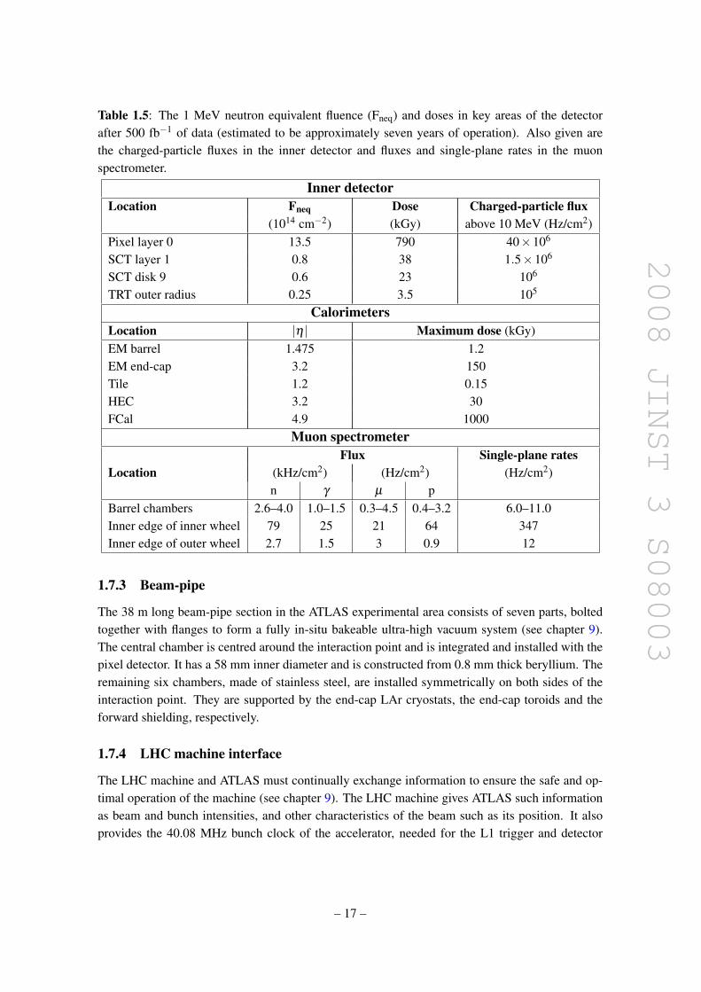
2008 JINST 3 S08003

Table 1.5: The 1 MeV neutron equivalent fluence (Fneq) and doses in key areas of the detectorafter 500 fb−1 of data (estimated to be approximately seven years of operation). Also given arethe charged-particle fluxes in the inner detector and fluxes and single-plane rates in the muonspectrometer.

Inner detectorLocation Fneq Dose Charged-particle flux

(1014 cm−2) (kGy) above 10 MeV (Hz/cm2)Pixel layer 0 13.5 790 40×106

SCT layer 1 0.8 38 1.5×106

SCT disk 9 0.6 23 106

TRT outer radius 0.25 3.5 105

CalorimetersLocation |η | Maximum dose (kGy)EM barrel 1.475 1.2EM end-cap 3.2 150Tile 1.2 0.15HEC 3.2 30FCal 4.9 1000

Muon spectrometerFlux Single-plane rates

Location (kHz/cm2) (Hz/cm2) (Hz/cm2)n γ µ p

Barrel chambers 2.6–4.0 1.0–1.5 0.3–4.5 0.4–3.2 6.0–11.0Inner edge of inner wheel 79 25 21 64 347Inner edge of outer wheel 2.7 1.5 3 0.9 12

1.7.3 Beam-pipe

The 38 m long beam-pipe section in the ATLAS experimental area consists of seven parts, boltedtogether with flanges to form a fully in-situ bakeable ultra-high vacuum system (see chapter 9).The central chamber is centred around the interaction point and is integrated and installed with thepixel detector. It has a 58 mm inner diameter and is constructed from 0.8 mm thick beryllium. Theremaining six chambers, made of stainless steel, are installed symmetrically on both sides of theinteraction point. They are supported by the end-cap LAr cryostats, the end-cap toroids and theforward shielding, respectively.

1.7.4 LHC machine interface

The LHC machine and ATLAS must continually exchange information to ensure the safe and op-timal operation of the machine (see chapter 9). The LHC machine gives ATLAS such informationas beam and bunch intensities, and other characteristics of the beam such as its position. It alsoprovides the 40.08 MHz bunch clock of the accelerator, needed for the L1 trigger and detector

– 17 –

2008 JINST 3 S08003

sub-systems. ATLAS provides information on total luminosity and luminosity per bunch obtainedfrom its luminosity detectors, and indications of the quality of the collisions based on informa-tion from the detector and from the beam conditions monitors (see chapter 3). The ATLAS beaminterlock system provides information on whether or not to safely inject or dump the beams, orto move from one mode of operation (e.g. filling) to the next (e.g. ramping). This information isexchanged through the detector control system information server, and dedicated hardware linksfor such critical information as beam permission signals and timing.

1.8 Outline of the paper

This paper is structured as follows. Chapter 2 summarises the key features of the solenoid andtoroid magnet system and the B-field determination methodology. The beam-line shielding and theexpected radiation levels are presented in chapter 3. This is followed, in chapters 4, 5, and 6, by thedescription of the inner detector, calorimetry, and muon spectrometer, respectively. The forwarddetectors, not shown in figure 1.1, are discussed in chapter 7. Chapter 8 outlines the hardwareaspects of the trigger and data acquisition systems. Chapter 9 then presents the main features of theinfrastructure in the ATLAS cavern, including the overall integration of the experiment, the sub-detector positioning strategy and the corresponding survey results, the services (including cables,pipes, gas and cooling systems, cryogenics, back-up power infrastructure, etc.), the beam-pipe, andthe access and maintenance scenarios. Chapter 10 presents an overview of the global performanceexpected from the ATLAS detector, as obtained from combined test-beam measurements and fromthe latest analysis results based on the large-scale simulations done for the commissioning of thecomputing system. Finally, chapter 11 briefly summarises the current status of installation andcommissioning, and the expectations for the ultimate completion of the detector and its operation.

– 18 –

2008 JINST 3 S08003

Chapter 2

Magnet system and magnetic field

This chapter begins with a brief description of the ATLAS magnet system (section 2.1), whichconsists of one solenoid and three toroids (one barrel and two end-caps). Section 2.2 proceeds witha description of the current understanding of the magnetic field across the whole apparatus. Thisincludes mapping of the solenoid field and first measurements of the barrel toroid field with theHall-probe system, as well as calculations to determine the detailed field map with the requiredaccuracy and performance specifications to be used in ATLAS simulation and reconstruction ap-plications.

2.1 Magnet system

ATLAS features a unique hybrid system of four large superconducting magnets. This magneticsystem is 22 m in diameter and 26 m in length, with a stored energy of 1.6 GJ. After approximately15 years of design, construction in industry, and system integration at CERN, the system is installedand operational in the underground cavern. This section presents the properties of the magnets andtheir related services. More details can be found in [2] for the solenoid.

Figure 1.1 shows the general layout, the four main layers of detectors and the four super-conducting magnets which provide the magnetic field over a volume of approximately 12,000 m3

(defined as the region in which the field exceeds 50 mT). The spatial arrangement of the coil wind-ings is shown in figure 2.1. The ATLAS magnet system, whose main parameters are listed intable 2.1, consists of:

• a solenoid (section 2.1.1), which is aligned on the beam axis and provides a 2 T axial mag-netic field for the inner detector, while minimising the radiative thickness in front of thebarrel electromagnetic calorimeter;

• a barrel toroid (section 2.1.2) and two end-cap toroids (section 2.1.3), which produce atoroidal magnetic field of approximately 0.5 T and 1 T for the muon detectors in the centraland end-cap regions, respectively.

The first conceptual design of the magnet system was sketched in the early 1990’s, and thetechnical design reports [3–6] were published in 1997. Regular project overviews and status reportsof design and production were made available [7, 8] throughout the design and manufacturing

– 19 –

2008 JINST 3 S08003

Figure 2.1: Geometry of magnet windings andtile calorimeter steel. The eight barrel toroidcoils, with the end-cap coils interleaved arevisible. The solenoid winding lies inside thecalorimeter volume. The tile calorimeter ismodelled (section 2.2.2) by four layers with dif-ferent magnetic properties, plus an outside re-turn yoke. For the sake of clarity the forwardshielding disk (section 3.2) is not displayed.

Figure 2.2: Bare central solenoid in the factoryafter completion of the coil winding.

phases. The cold-mass and cryostat integration work began in 2001. The first barrel toroid coilwas lowered in the cavern in fall 2004, immediately followed by the solenoid (embedded inside theLAr barrel calorimeter). The remaining seven barrel-toroid coils were installed in 2004 and 2005,and the end-cap toroids in the summer of 2007.

2.1.1 Central solenoid

The central solenoid [2] is displayed in figure 2.2, and its main parameters are listed in table 2.1.It is designed to provide a 2 T axial field (1.998 T at the magnet’s centre at the nominal 7.730 kAoperational current). To achieve the desired calorimeter performance, the layout was carefullyoptimised to keep the material thickness in front of the calorimeter as low as possible, resultingin the solenoid assembly contributing a total of ∼ 0.66 radiation lengths [9] at normal incidence.This required, in particular, that the solenoid windings and LAr calorimeter share a common vac-uum vessel, thereby eliminating two vacuum walls. An additional heat shield consisting of 2 mmthick aluminium panels is installed between the solenoid and the inner wall of the cryostat. Thesingle-layer coil is wound with a high-strength Al-stabilised NbTi conductor, specially developedto achieve a high field while optimising thickness, inside a 12 mm thick Al 5083 support cylin-der. The inner and outer diameters of the solenoid are 2.46 m and 2.56 m and its axial lengthis 5.8 m. The coil mass is 5.4 tonnes and the stored energy is 40 MJ. The stored-energy-to-massratio of only 7.4 kJ/kg at nominal field [2] clearly demonstrates successful compliance with thedesign requirement of an extremely light-weight structure. The flux is returned by the steel of theATLAS hadronic calorimeter and its girder structure (see figure 2.1). The solenoid is charged anddischarged in about 30 minutes. In the case of a quench, the stored energy is absorbed by the en-thalpy of the cold mass which raises the cold mass temperature to a safe value of 120 K maximum.Re-cooling to 4.5 K is achieved within one day.

– 20 –

2008 JINST 3 S08003

Table 2.1: Main parameters of the ATLAS magnet system.Property Feature Unit Solenoid Barrel toroid End-cap toroidsSize Inner diameter m 2.46 9.4 1.65

Outer diameter m 2.56 20.1 10.7Axial length m 5.8 25.3 5.0Number of coils 1 8 2 × 8

Mass Conductor t 3.8 118 2 × 20.5Cold mass t 5.4 370 2 × 140Total assembly t 5.7 830 2 x 239

Coils Turns per coil 1154 120 116Nominal current kA 7.73 20.5 20.5Magnet stored energy GJ 0.04 1.08 2 x 0.25Peak field in the windings T 2.6 3.9 4.1Field range in the bore T 0.9–2.0 0.2–2.5 0.2–3.5

Conductor Overall size mm2 30 x 4.25 57 x 12 41 x 12Ratio Al:Cu:NbTi 15.6:0.9:1 28:1.3:1 19:1.3:1Number of strands (NbTi) 12 38–40 40Strand diameter (NbTi) mm 1.22 1.3 1.3Critical current (at 5 T and 4.2 K) kA 20.4 58 60Operating/critical-current ratio at 4.5 K % 20 30 30Residual resistivity ratio (RRR) for Al > 500 > 800 > 800Temperature margin K 2.7 1.9 1.9Number of units × length m 4 × 2290 8 × 4 × 1730 2 × 8 × 2 × 800Total length (produced) km 10 56 2 x 13

Heat load At 4.5 K W 130 990 330At 60–80 K kW 0.5 7.4 1.7Liquid helium mass flow g/s 7 410 280

The electromagnetic forces are counteracted by the combination of the coil and warm-to-coldmechanical support, which maintains the concentricity of the windings. All solenoid services passthrough an S-shaped chimney at the top of the cryostat, routing the service lines to the correspond-ing control dewar (section 2.1.4.2).

The coil was manufactured and pre-tested in the factory [10], came to CERN for integration inthe LAr cryostat, underwent an on-surface acceptance test in its semi-final configuration [11], andwas installed in its final central position in ATLAS in October 2005. The one week cool-down anda commissioning test up to nominal field were successfully completed in the summer of 2006 [12].The solenoid is now ready for detector operation.

2.1.2 Barrel toroid

The main parameters of the magnet are listed in table 2.1. The cylindrical volume surrounding thecalorimeters and both end-cap toroids (see figure 1.1) is filled by the magnetic field of the barreltoroid, which consists of eight coils encased in individual racetrack-shaped, stainless-steel vacuumvessels (see figure 2.3). The coil assembly is supported by eight inner and eight outer rings ofstruts. The overall size of the barrel toroid system as installed is 25.3 m in length, with inner andouter diameters of 9.4 m and 20.1 m, respectively.

– 21 –

2008 JINST 3 S08003

Figure 2.3: Barrel toroid as installed in the underground cavern; note the symmetry of the support-ing structure. The temporary scaffolding and green platforms were removed once the installationwas complete. The scale is indicated by the person standing in between the two bottom coils.Also visible are the stainless-steel rails carrying the barrel calorimeter with its embedded solenoid,which await translation towards their final position in the centre of the detector.

The conductor and coil-winding technology is essentially the same in the barrel and end-captoroids; it is based on winding a pure Al-stabilised Nb/Ti/Cu conductor [13] into pancake-shapedcoils, followed by vacuum impregnation.

The cold-mass integration [14] and the cryostat integration [15] were performed at CERNover a period of approximately three years, and were completed in summer 2005. In parallel, allcoils successfully underwent on-surface acceptance test procedures [16]. Cool down and testingof the barrel toroid in the cavern took place in 2006. The cool down of the 360-tonne cold massto 4.6 K takes five weeks. The test programme included normal ramps, up to nominal current (in2 hours) followed by either a slow dump (in 2 hours) or a fast dump (in 2 minutes) in the caseof a provoked quench. The ultimate test sequence that proved the system’s health is shown infigure 2.4. The magnet current is raised in steps up to its nominal value of 20.5 kA and then finallyup to 21.0 kA, demonstrating the ability of the system to withstand at least an additional 500 A.The current is then allowed to decay back to its design value; the magnet is finally turned off by adeliberate fast dump. After re-cooling the cycle was repeated, demonstrating that no degradationhad occurred up to the nominal operating current. During a fast dump, triggered either manually orby the quench detection system, the stored energy of 1.1 GJ is absorbed by the enthalpy of the coldmass following the activation of four quench heaters per coil and in all eight coils, which forcesthe entire magnet into the normal conducting state within less than two seconds. This leads to avery safe global cold mass temperature of about 58 K and a hot-spot temperature in the windings ofabout 85 K maximum. The uniform quench heating system also ensures that the internal voltage inthe toroid is kept at a low value of about 70 V. After a fast dump the magnet cooling system needs

– 22 –

2008 JINST 3 S08003

Time (min.)0 50 100 150 200 250 300

Cur

rent

(kA

)

0

2

4

6

8

10

12

14

16

18

20

22

Figure 2.4: Time history of the barrel toroidcurrent during an excitation test up to 102%of the nominal value. The current drops backto zero within two minutes of the deliberately-provoked quench.

Figure 2.5: End-cap toroid cold mass insertedinto the cryostat. The eight flat, square coilunits and eight keystone wedges (with the cir-cular holes) are visible.

about 50 hours to re-cool the toroid to 4.6 K whereafter normal operation can re-start. The detailsof the coil testing are published elsewhere, in [17] for the first coil, in [18] for an overall summary,and in [19] and [20] for quench behaviour and quench losses, respectively.

The net Lorentz forces of approximately 1400 tonnes per coil directed inwards and the self-weight of the toroids are counteracted by the warm structure of Al-alloy struts mounted in betweenthe eight coils. However, the barrel toroid structure still deflects significantly under its own weight.After release of the temporary support structure and systematic loading of the toroid with its ownweight of 830 tonnes and the additional 400 tonnes of weight of the muon chambers, the final shapeof the toroid bore was designed to be cylindrical. The toroid coils were installed in calculated posi-tions on an oval, longer by 30 mm in the vertical direction, to allow for structure deflection duringload transfer from the temporary support structure. Since the release and removal of the installa-tion supports, the upper edge of the toroid moved down by about 26 mm, which demonstrates thatthe design values had been well established and that the installation was precise to within a fewmillimetres.

The installation of the barrel toroid in the ATLAS cavern commenced in October 2004. Ittook about 11 months to install the complete toroid, as depicted in figure 2.3. This is discussedin more detail in section 9.6 within the context of the overall ATLAS installation, for which thistoroid installation phase was one of the most demanding ones. The overall structure design andinstallation experience are reported in [21].

– 23 –

2008 JINST 3 S08003

2.1.3 End-cap toroids

The main parameters of the two end-cap toroids are listed in table 2.1. These toroids generatethe magnetic field required for optimising the bending power in the end-cap regions of the muonspectrometer system. They are supported off and can slide along the central rails, which facilitatesthe opening of the detector for access and maintenance (see section 9.5.1). Each end-cap toroidconsists of a single cold mass built up from eight flat, square coil units and eight keystone wedges,bolted and glued together into a rigid structure to withstand the Lorentz forces (see figure 2.5).Design details are given elsewhere [22], and the production in industry of the coil modules andvacuum vessels is described in [23].

The cold masses were assembled and inserted into their cryostats at CERN. Figure 2.5 showsthe first end-cap toroid interior just prior to the closing of the vacuum vessel. A crucial step in theintegration process is the adjustment of the cold mass supports [24]. The weights of cold mass andvacuum vessel are 140 and 80 tonnes respectively. With the exception of windings, coil supports,and bore tube, the entire structure is made of Al alloy. With a weight of 240 tonnes, the end-captoroids were some of the heaviest objects to be lowered into the cavern.

The end-cap-toroid cold masses will each be subject to a Lorentz force of 240 tonnes, pushingthem against the stops mounted on the eight barrel toroid coils. Achieving the correct sharing of theforces in the axial tie-rods has therefore been a critical design goal. Prior to their installation in thecavern in summer 2007, both end-cap toroids passed tests at 80 K to check the magnet mechanicsand electrical insulation after thermal shrinkage. Once the end-cap toroids are powered in serieswith the barrel toroid, the peak stress in the barrel-toroid windings, in the areas where the magneticfields overlap, will increase by about 30%. After a four-week cooldown, both end-cap toroids weresuccessfully tested at half current, albeit one at a time and in stand-alone mode. The final tests atfull field will take place in the spring of 2008, after the installation of the shielding disks and withthe end-cap calorimeters at their nominal position.

2.1.4 Magnet services

2.1.4.1 Vacuum system

The insulating vacuum is achieved with diffusion pumps directly attached to the barrel and theend-cap toroids, two per coil for all toroids, each with a capacity of 3000 m3/h. In addition, tworoughing and three backing pumps are used in the low stray-field area at the cavern wall. Undernormal conditions, with a leak rate less than 10−4 mbar · l/s, a single pump would be sufficient.However, for redundancy and in order to minimise detector down-time, extra pumping units wereinstalled. Since the solenoid is installed inside the cryostat of the LAr barrel calorimeter, theinsulation vacuum is controlled by the LAr cryogenic system (section 9.4.5) rather than by themagnet control system (see section 2.1.4.4).

2.1.4.2 Cryogenics

The overall cryogenic systems in ATLAS are described in section 9.4. Here, details are providedon the system specific to the magnets.

– 24 –

2008 JINST 3 S08003

Figure 2.6: Layout of the magnet cryogenics system in the surface hall (compressors) and servicecavern (shield refrigerator and helium liquefier). They deliver cold gas and liquid to the distributionvalve box in the experimental cavern, from which the solenoid and the toroid proximity cryogenicsare fed (see figure 2.7).

The overall magnet cryogenic system is divided into external, proximity, and internal cryo-genics, which are connected via transfer lines. The lines serving the solenoid and barrel toroidremain fixed, whereas those of the end-cap toroids are partially flexible, as these toroids have to bemoved to access the calorimeters and inner detector for maintenance and repairs (section 9.7).

The layout of the various cryogenic systems is shown in figure 2.6. The external cryogenicsconsist of two refrigerators (the main refrigerator and the shield refrigerator), a distribution transferline, and a distribution valve box. The main refrigerator cold box has a refrigeration capacity of6 kW at 4.5 K equivalent, while the shield refrigerator cold box has a refrigeration capacity of20 kW at 40–80 K.

The gas buffers are located on the surface with the refrigerator compressors, while the refrig-erator cold boxes are installed in the USA15 side cavern. The common distribution transfer line

– 25 –

2008 JINST 3 S08003

Figure 2.7: Left: Layout of underground service connections to the solenoid and toroid systems.The two large helium dewars can be seen on the side of the main cavern. Also shown are the fixedcryogenic lines supplying the solenoid and the cryo-ring for the barrel toroid coils at the top. Thecryogenics lines in the flexible chains supply the two end-cap toroids and follow them wheneverthey move for detector access and maintenance. Right: schematic of the liquid-helium supply inthe barrel toroid. The cryo-ring contains six standard sectors; a bottom sector with a valve boxwhere the input flow per coil is measured and controlled; and the top sector where all lines cometogether and which is connected to the current lead cryostat.

makes the link to the distribution valve box in the main cavern. All proximity cryogenics equip-ment, including the storage dewar, cold pumps, cryostat phase separator, and distribution valvebox (except for the valve unit of the solenoid) are positioned near the wall of the main cavern, asschematically shown in figure 2.7 (left).

The distribution valve box channels the fluids to two independent proximity cryogenic sys-tems, one for the toroids (barrel cryo-ring and two end-caps) and one for the solenoid. For thetoroids, there is a storage dewar with a capacity of 11,000 litres of liquid helium. There also exist adistribution valve box, a phase separator dewar with two centrifugal pumps and a storage capacityof 600 litres of liquid helium. The solenoid has a control dewar with a storage capacity of 250 litresof liquid helium, positioned at the top of the detector.

The proximity cryogenic equipment supplies coolant to the magnet internal cryogenics, whichconsist mainly of cooling pipes attached to the cold mass and the thermal shield. The aluminiumcooling tubes are either welded to the outer surface of the Al-alloy support cylinder (solenoid) orembedded and glued inside and on top of the Al-alloy coil casings enclosing the pancake coils(toroids).

The toroids are cooled with a forced flow of boiling helium, which enters the magnets fromthe top. In the case of the barrel toroid (see figure 2.7), helium is supplied from the current leadcryostat positioned on the top sector, runs down to the distribution valve box at floor level with

– 26 –

2008 JINST 3 S08003

eight control valves regulating the flow in the eight coils, then goes up and enters the eight coilsseparately, while the return line returns to the top. A total of 1200 g/s of slightly sub-cooled liquidhelium is circulated by means of centrifugal pumps, which take the liquid from the phase separatordewar. The system is equipped with two pumps for redundancy. The second pump is called intooperation if the first one fails. The liquid helium in the storage dewar will be used in the event of afailure with the main refrigerator to provide the required cooling capacity to safely ramp down thetoroids over a two-hour period.

The solenoid, with a cold mass of approximately five tonnes, is cooled by a direct Joule-Thompson flow from the main refrigerator and is slightly sub-cooled via a heat exchanger in the250 litre helium control dewar.

The flow in the solenoid and the ten toroid cold masses is controlled individually to cope withvariations in flow resistance and to guarantee helium quality in all coils. Given that the end-captoroids and solenoid each have a single cold mass, there is a single flow control and the branchesof cooling pipes (two for the solenoid and sixteen for each end-cap toroid) are arranged in parallel.

2.1.4.3 Electrical circuits

The three toroids are connected in series to the 20.5 kA/16 V power supply shown schematicallyin figure 2.8 (left). They are however individually voltage-protected by the two diode/resistor ramp-down units. The electrical circuit of the central solenoid is similar and shown in figure 2.8 (right).It has a 8 kA/8 V power supply. The power supply, switches, and diode/resistor units are locatedin the side cavern and approximately 200 m of aluminium bus-bars provide the connections tothe magnets in the cavern. Ramping up is accomplished at a rate of 3 A/s, leading to a max-imum ramp-up time of two hours. In the case of a slow dump, the magnets are de-energisedacross the diode/resistor units in about 2.5 hours. Quench detection is by classical bridge connec-tions across the entire barrel toroid, across the end-cap toroids and across the solenoid, as well asacross individual coils, using differential voltage measurements with inductive voltage compensa-tion.

There is a six-fold redundancy in the toroid quench detection grouped in two physically-separated units and cable routings. Quench protection is arranged by firing heaters in all toroidcoils so that a uniform distribution of the cold-mass heating is achieved. Given the normal-zonepropagation of 10–15 m/s, a toroid coil is switched back to the normal state within 1–2 seconds.As for the quench detection, the quench-protection heater circuits including power supply, cabling,and heaters embody a two-fold redundancy. A similar system is used for the solenoid. An overviewof the magnet services can be found in [25].

2.1.4.4 Magnet controls

A magnet control system steers and executes automatically the various running modes of the mag-net system. Its implementation is realised as part of the overall ATLAS detector control system,as described in section 8.5. The hardware designs rely on a three-layer model, using distributedinput/output connected via field-networks or directly by wiring to a process-control layer, the lastlayer being the supervisor.

– 27 –

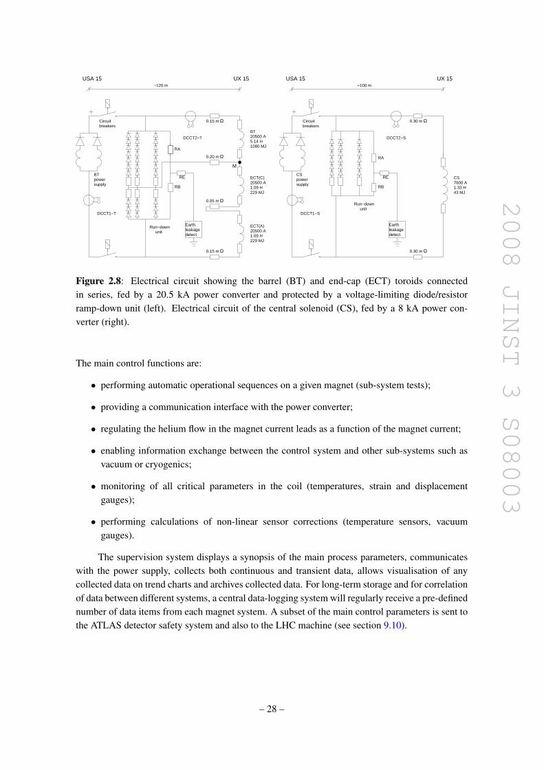
2008 JINST 3 S08003

BT20500 A5.14 H1080 MJ

ECT(A)20500 A1.09 H229 MJ

ECT(C)20500 A1.09 H229 MJ

CS7600 A1.33 H43 MJ

CSpowersupply

Earthleakagedetect

BTpowersupply

Earthleakagedetect

Run−down unit

Run−down unit

0.20 m Ω

~

0.15 m

DCCT2−T

~120 m ~100 m

DCCT2−S

DCCT1−SDCCT1−T

RB

RE

RA

RA

RE

RB

USA 15 UX 15 USA 15 UX 15

Circuit Circuit

M

Ω

0.05 m

0.15 m 0.30 m

0.30 m

Ω

Ω Ω

Ω

breakers breakers

Figure 2.8: Electrical circuit showing the barrel (BT) and end-cap (ECT) toroids connectedin series, fed by a 20.5 kA power converter and protected by a voltage-limiting diode/resistorramp-down unit (left). Electrical circuit of the central solenoid (CS), fed by a 8 kA power con-verter (right).

The main control functions are:

• performing automatic operational sequences on a given magnet (sub-system tests);

• providing a communication interface with the power converter;

• regulating the helium flow in the magnet current leads as a function of the magnet current;

• enabling information exchange between the control system and other sub-systems such asvacuum or cryogenics;

• monitoring of all critical parameters in the coil (temperatures, strain and displacementgauges);

• performing calculations of non-linear sensor corrections (temperature sensors, vacuumgauges).

The supervision system displays a synopsis of the main process parameters, communicateswith the power supply, collects both continuous and transient data, allows visualisation of anycollected data on trend charts and archives collected data. For long-term storage and for correlationof data between different systems, a central data-logging system will regularly receive a pre-definednumber of data items from each magnet system. A subset of the main control parameters is sent tothe ATLAS detector safety system and also to the LHC machine (see section 9.10).

– 28 –

2008 JINST 3 S08003

2.2 Magnetic field determination

The specifications on the determination of the magnetic field (section 2.2.1) are rather differentin the inner detector (ID) and the muon spectrometer. In the ID cavity, the driving consider-ation is the absolute accuracy of the momentum scale. In the muon spectrometer, the field ishighly non-uniform: residual bending-power uncertainties, if large enough, would translate pri-marily into degraded muon momentum resolution. Detailed magnetic modelling (section 2.2.2)and novel instrumentation (section 2.2.3) have allowed a high-precision mapping of the solenoidfield (section 2.2.4) as well as a preliminary experimental validation of the field measurement andreconstruction strategy in the muon spectrometer (section 2.2.5). Studies are in progress to com-bine magnetic models with field measurements into an overall field map for ATLAS data-taking(section 2.2.6).

2.2.1 Performance specifications and measurement concepts

In the inner detector, the systematic error affecting the momentum measurement of charged tracksis dominated by the relative alignment of detector components and by bending-power uncertain-ties, the former being the more demanding. A high-precision measurement of the W -boson massis clearly the most challenging goal for such measurements: a lepton from W decay carries typi-cally a transverse momentum of 40 GeV, resulting in a sagitta of approximately 1 mm as the leptontraverses the ID cavity. The systematic alignment uncertainties in the ID are unlikely to improvebeyond the 1 µm level or 0.1% of the sagitta. This suggests setting a target of ∼ 5× 10−4 forthe fractional bending power uncertainty, so that it remains negligible in the determination of theabsolute momentum scale. Such stringent requirements can only be achieved reliably by in-situmapping, using dedicated instrumentation inside the ID cavity, with all the relevant magnetic ma-terials in place and just before the final installation of the ID itself. Eventual long-term drifts of theabsolute scale will be detected to a much higher accuracy using permanently installed NMR probes.

In the muon spectrometer, the expected sagitta is approximately 0.5 mm for a muon witha momentum of 1 TeV. The extraction of the momentum from the Monitored Drift Tube (MDT)chamber measurements requires a precise knowledge of the field integral between consecutivechambers along the muon trajectory. Because the field gradient can reach 1 mT/mm, local bending-power uncertainties translate into fluctuations of the momentum scale from one region in space toanother, adding in quadrature to the overall momentum resolution. In addition, the interpretation,in terms of spatial coordinates, of the drift time measured in the MDT’s is sensitive to the localelectric and magnetic fields experienced by the ionisation electrons in each tube. The correspondingfunctional requirements are extensively discussed in [26] and summarised in table 2.2.

For a given muon trajectory, three sources of uncertainty affect the measured curvature: fieldmeasurement errors; accuracy on the relative position of muon chambers and magnet coils; andtrajectory measurement errors, in particular along the direction of MDT wires. For the purposeof setting specifications, it has been required (somewhat arbitrarily) that the combined effect ofthese sources degrade the momentum resolution by no more than 5% in relative terms; each sourceshould then contribute no more than ∼3% of fractional resolution degradation, anywhere in thespectrometer volume.

– 29 –

2008 JINST 3 S08003

Table 2.2: Summary of magnetic-field-related performance specifications in the muon spectrome-ter. The quoted spread reflects the η−φ variations in field gradient and/or strength.

Criterion Bending-power accuracy MDT drift propertiesPerformance ∆σpT /σpT < 5% overall Single-wire resolution degraded by < 5%Field measurement accuracy ∆Bφ /Bφ < 2 – 5 ×10−3 ∆Bx,y,z < 4 mT (relative over chamber)Reconstructed position of toroid ∆R∼ 1 – 12 mm, R∆φ ∼ 1 – 6 mm, -conductors with respect to MDT tower ∆z∼ 2 – 30 mmMuon chamber 2nd-coordinate resolution 1.7–5.5 mm 6 to ∼ 100 mm

In-situ mapping of the spectrometer by conventional techniques would have been impracticalbecause of the rapidly-varying field and very large volume. Instead, the muon system is equippedwith a total of approximately 1840 B-field sensors; their readings are compared with magneticsimulations and used for reconstructing the field in space. This strategy was shown [27] to meet thefield-map specifications above, provided the B-sensor readings, after correcting for perturbationsinduced by magnetic materials, are accurate to∼ 1 mT (absolute) and the field direction is measuredto within ± 3 mrad.

2.2.2 B-field modelling

The total field in the ID cavity, the calorimeters, and the muon spectrometer is computed as thesuperposition of the Biot-Savart contributions of all magnet windings (see figure 2.1) with thoseof the magnetised calorimeter and with the localised perturbations induced by other ferromagneticstructures. In order to reach the required accuracy, the calculation combines numerical integrationof the contributions of the solenoid, barrel-toroid and end-cap-toroid windings with finite-elementmodelling of magnetic structures.

The solenoid conductor model is described in section 2.2.4. The magnetised steel (tilecalorimeter and solenoid flux-return girder), which surrounds the ID cavity, is predicted to modifythe field by 4.1% at the geometrical centre of the coil. At nominal current, the total measured fieldis 1.998 T at the interaction point, and drops steeply from ∼ 1.8 T at z = 1.7 m to ∼ 0.9 T at theend of the ID cavity (see figure 2.9).

The toroid windings are, at this stage, described using their nominal geometry. The meshdensity of the stored field map is tailored to the local field gradient to ensure an accurate represen-tation of field variations (as also done for the solenoid). Depending on the radius R and azimuth φ ,the field varies from 0.15 T to 2.5 T, with an average value of 0.5 T, in the barrel region, andfrom 0.2 to 3.5 T in the end-cap region [28]. The analysing performance of the toroid system canbe roughly quantified by the field integral experienced by particles originating from the interactionpoint and propagating in a straight line (the ultimate criterion is the momentum resolution: a zerofield integral does not necessarily imply infinite resolution). This available bending power is shownin figure 2.10 as a function of |η |. It shows good magnetic field coverage up to |η | ∼ 2.6. Theregions with low field integral, between |η | = 1.4 and |η | = 1.6, correspond to trajectories in theplane of an end-cap coil or of a barrel coil, where the fringe field of one magnet largely cancels thebending power of the other.

– 30 –

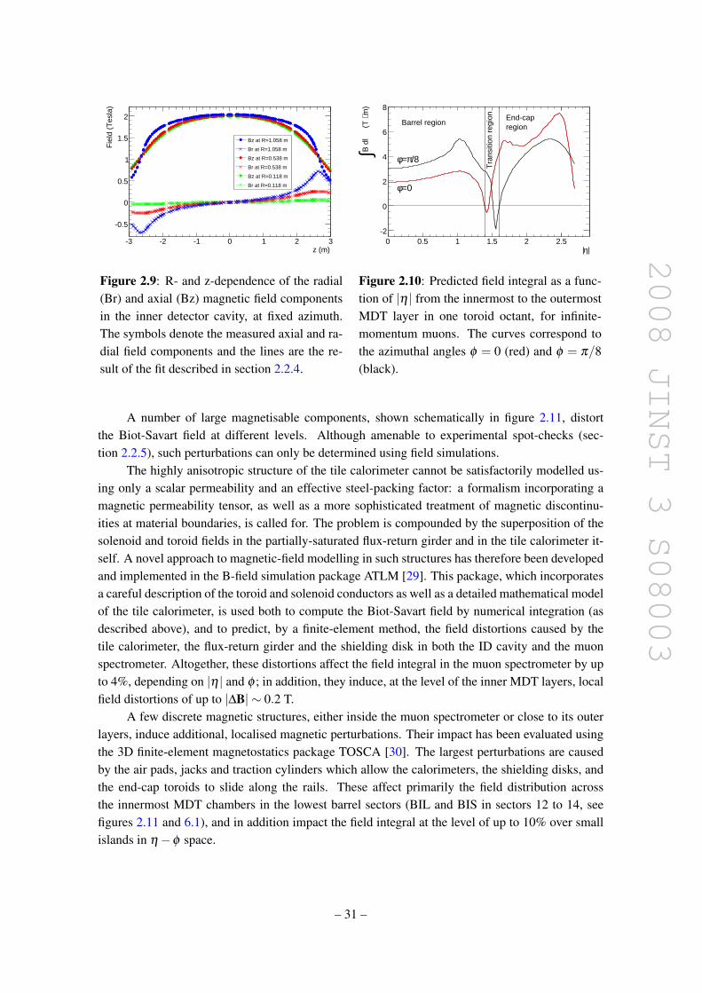
2008 JINST 3 S08003

z (m)-3 -2 -1 0 1 2 3

Fie

ld (

Tes

la)

-0.5

0

0.5

1

1.5

2

Bz at R=1.058 m

Br at R=1.058 m

Bz at R=0.538 m

Br at R=0.538 m

Bz at R=0.118 m

Br at R=0.118 m

|η|0 0.5 1 1.5 2 2.5

m)

⋅B

dl

(T

∫

-2

0

2

4

6

8

Barrel regionregionEnd-cap

Tra

nsiti

on r

egio

n

=0φ

/8π=φ

Figure 2.9: R- and z-dependence of the radial(Br) and axial (Bz) magnetic field componentsin the inner detector cavity, at fixed azimuth.The symbols denote the measured axial and ra-dial field components and the lines are the re-sult of the fit described in section 2.2.4.

Figure 2.10: Predicted field integral as a func-tion of |η | from the innermost to the outermostMDT layer in one toroid octant, for infinite-momentum muons. The curves correspond tothe azimuthal angles φ = 0 (red) and φ = π/8(black).

A number of large magnetisable components, shown schematically in figure 2.11, distortthe Biot-Savart field at different levels. Although amenable to experimental spot-checks (sec-tion 2.2.5), such perturbations can only be determined using field simulations.

The highly anisotropic structure of the tile calorimeter cannot be satisfactorily modelled us-ing only a scalar permeability and an effective steel-packing factor: a formalism incorporating amagnetic permeability tensor, as well as a more sophisticated treatment of magnetic discontinu-ities at material boundaries, is called for. The problem is compounded by the superposition of thesolenoid and toroid fields in the partially-saturated flux-return girder and in the tile calorimeter it-self. A novel approach to magnetic-field modelling in such structures has therefore been developedand implemented in the B-field simulation package ATLM [29]. This package, which incorporatesa careful description of the toroid and solenoid conductors as well as a detailed mathematical modelof the tile calorimeter, is used both to compute the Biot-Savart field by numerical integration (asdescribed above), and to predict, by a finite-element method, the field distortions caused by thetile calorimeter, the flux-return girder and the shielding disk in both the ID cavity and the muonspectrometer. Altogether, these distortions affect the field integral in the muon spectrometer by upto 4%, depending on |η | and φ ; in addition, they induce, at the level of the inner MDT layers, localfield distortions of up to |∆B| ∼ 0.2 T.

A few discrete magnetic structures, either inside the muon spectrometer or close to its outerlayers, induce additional, localised magnetic perturbations. Their impact has been evaluated usingthe 3D finite-element magnetostatics package TOSCA [30]. The largest perturbations are causedby the air pads, jacks and traction cylinders which allow the calorimeters, the shielding disks, andthe end-cap toroids to slide along the rails. These affect primarily the field distribution acrossthe innermost MDT chambers in the lowest barrel sectors (BIL and BIS in sectors 12 to 14, seefigures 2.11 and 6.1), and in addition impact the field integral at the level of up to 10% over smallislands in η−φ space.

– 31 –

2008 JINST 3 S08003

Figure 2.11: Sources of magnetic perturbationsinduced by metallic structures in or near themuon spectrometer.

Figure 2.12: Schematic representation of themagnetic-sensor layout and coil deformationmodel, used to reconstruct the magnetic fieldinside a barrel octant. The MDT nomenclatureis defined in tables 6.3 and 6.4 (see section 6.3).

The field perturbations caused in the outside MDT layers by the massive steel frame andplatforms (HS structure described in section 9.5), which surround the detector, range from |∆B| ∼2 mT up to ∼ 50 mT and rapidly decrease as one moves inwards from the outer to the middlechamber layer. While their impact on B-sensor readings and MDT drift properties does need to betaken into account, they barely affect the bending power, except possibly in a few narrow regions.

The other components in figure 2.11 have much less of an impact because either they lie ina low-field region, they intercept a very small fraction of the end-cap muons, or they are made ofstainless steel with a high-field relative permeability very close to 1.

2.2.3 Magnetic field instrumentation and reconstruction

2.2.3.1 B-field sensors

The inner detector is equipped with four NMR probes fixed to the wall of the inner warm vesselnear z∼ 0 and equally spaced in azimuth. These probes measure the field strength with an accuracyof around 0.01 mT and will remain in place to monitor the ID field strength throughout the lifetimeof ATLAS.

– 32 –

2008 JINST 3 S08003

Because NMR probes only measure |B| and because they cease functioning in a gradient ofa few tenths of mT/cm, the solenoid mapper, described in section 2.2.4, and the muon chambersare equipped instead with 3D Hall cards [31, 32]. These consist of a rigid printed-circuit boardcarrying a small glass cube, with a Hall probe on each of three orthogonal faces to measure eachfield component. Every card includes its own readout electronics, as well as a thermistor for localtemperature compensation.

All the Hall cards were calibrated in a highly uniform field monitored by a NMR probe. Theachieved absolute Hall-card accuracy on |B| is 0.2 mT up to |B|= 1.4 T and 1 mT up to 2.5 T; andthe angular accuracy achieved on the measured field direction is 2 mrad.

2.2.3.2 B-field reconstruction

In an air-core magnet, the magnetic field can in principle be calculated by direct application ofthe Biot-Savart law, once the geometry of all conductors is known and assuming material-inducedmagnetic perturbations are negligible. In practice however, the conductor position and shape areknown only approximately, owing to fabrication tolerances and to deformations of the magnetstructure under gravitational and magnetic loads. The exact location of each magnet coil, as wellas the relative positions of the end-cap and barrel toroids, will be reproducible, after a power cycleor an access period, to a finite precision only. Therefore, the field must be measured under runningconditions, with all detector components in place and under the mutual influence of the differentmagnets and magnetic structures.

The muon spectrometer is equipped with an array of approximately 1730 Hall cards, whichremain mounted permanently and precisely on the MDT chambers and continuously measure allthree field components (an additional 64 cards are mounted on the inner and outermost faces ofthe end-cap toroid cryostats to complement the MDT sensor system in the forward region). TwoNMR probes, installed at low-gradient locations in the barrel toroid, complement the system, withthe aim of detecting eventual long-term drifts in the response of the Hall cards. The 3-D sensorreadings are compared with field calculations which include both the contributions of the magnetwindings and those of nearby magnetised structures, and are used for reconstructing the positionand the shape of the toroid conductors with respect to the muon chambers (see figure 2.12). Oncethe geometry of the coils is known, the field can be calculated anywhere in the muon spectrometer.Simulation studies using a simplified coil deformation model have shown that the magnetic fieldcan be reconstructed to a relative accuracy of 0.2% [27].

2.2.4 Solenoid-mapping measurements

2.2.4.1 Mapping campaign

The field was mapped [33] in August 2006 by a machine, which scanned a Hall-card array over avolume slightly larger than that now occupied by the inner detector. During this mapping campaign,the barrel and end-cap calorimeters were all in their final positions. Although the shielding diskswere not yet installed, their differential contribution is small enough (< 0.2 mT in the ID trackingvolume) that it can be reliably accounted for later. The same is true of corrections for the absenceof toroid excitation during mapping.

– 33 –

2008 JINST 3 S08003

Mapping data were recorded with solenoid currents of 7730, 7850, 7000, and 5000 A, witha final set of data back at the nominal operating current of 7730 A. Each data set contains at least20,000 points, and is sufficient by itself to fit the field with negligible statistical uncertainty. Eachmap took about four hours, during which the solenoid current remained stable to within 0.1 A, asconfirmed by the NMR probes.

2.2.4.2 Mapper geometry, survey and auto-calibration

The mapping machine had four arms mounted on a common axle in a windmill configuration, withtwelve Hall cards on each arm, at radii ranging from 0.118 to 1.058 m, which directly measuredthe field components Bz, BR and Bφ . The machine could be rotated around its axle and translatedin z along the ID rails by means of pneumatic motors. Optical encoders allowed control of themapper movements and readout of its stop positions with an accuracy of 0.1 mm. A number ofsurveys were necessary to determine the positions of each individual Hall sensor for all possiblelongitudinal mapper positions and azimuthal settings of the windmill arms. After combining all theinformation, the estimated overall accuracy on the position of a map point in the cryostat coordinatesystem is approximately 0.3 mm.

The redundancy and internal consistency of the mapping measurements makes it possible toextract individual probe misalignments from the data themselves to an accuracy of±0.1 mrad. Thestrong constraints from Maxwell’s equations on physically realisable fields in the absence of anycurrent sources or magnetic materials, combined with the fact that the field at the origin can bealmost completely determined from the measurements of a single Hall probe, allow all three probealignment angles to be determined and the Bz component to be normalised to a common scale forall probes.

The NMR probes, which were operational throughout the field-mapping campaigns, are usedto set the overall scale of the Hall sensors with an accuracy of about 0.4 mT, the limitation comingfrom the extrapolation uncertainty from the mapper arms out to the position of the NMR probes.The NMR data also show that there is negligible hysteresis in the solenoid system: the field at7730 A remained constant within ±0.01 mT from the first excitation cycle onwards, provided thatthis current was approached from below. A small saturation effect is visible in the NMR data, withthe field at 5000 A being 0.34 mT higher than would be expected by simply scaling down from7730 A.

2.2.4.3 Map fitting

Using the measured magnet current and a detailed model of the solenoid geometry, the Biot-Savartlaw is integrated to produce a field model which should account for most of the measured field.The conductor model is based on engineering drawings, with as many parameters as possible takenfrom surveys of the as-built solenoid. The coil cross-section is assumed to be perfectly circular. Thewinding was mechanically assembled from four separate sections, each with a slightly differentaverage pitch, and joined together by welds which are represented electrically by turns havingjust under twice the average pitch. Also modelled are the welds at the coil ends and the returnconductor which runs axially along the outside of the support cylinder. The expected distortion

– 34 –

2008 JINST 3 S08003

Table 2.3: Typical fit results of solenoid-mapping measurement at 7730 A.Fitted parameters Fit resultsScale factors in conductor model (R scale, z scale) = 0.9993, 1.0012Fitted offsets from solenoid centre to centre of cryostat (∆x,∆y,∆z) = 0.26, -2.42, 0.51 (mm)Fitted rotations of solenoid around cryostat x and y axes (θx,θy) = -0.08, 0.19 (mrad)Resulting fit residuals σ(∆Bz,∆BR, ∆Bφ ) = 0.44, 0.35, 0.30 (mT)

of the solenoid, relative to the room-temperature survey and caused by thermal shrinkage andmagnetic pressure, is also taken into account.

The geometrical fit to the mapping data has 11 free parameters. Two overall scale factorsallow fine tuning of the conductor model: one common to all longitudinal dimensions, and anindependent one for the radial dimension. Five more free parameters quantify the three offsetsand two rotations of the conductor relative to the mapper coordinate system. The calorimeter-steelcontribution is modelled by a Fourier-Bessel series with four terms. These parameters are deter-mined by minimising a χ2 function which includes the longitudinal and radial field componentsat all mapped points. The RMS residuals of the geometrical fit alone are just over 0.5 mT. Thisfield model is further improved by parametrising the difference between the data and the geomet-rical model with a general series which can represent any field obeying Maxwell’s equations. Thisbrings the residuals down to about 0.4 mT, as shown in table 2.3.

Systematic uncertainties are estimated by fitting to several representative data sets under vary-ing assumptions, with and without implementing various corrections (such as Hall-card alignment,z-dependent carriage tilt, residual perturbations induced by slightly magnetic mapper components,number of Fourier-Bessel terms etc.). The geometrical scale factors emerge as very close to unity(table 2.3), suggesting that the coil survey data are well understood. The fitted offsets and rotationswith respect to the centre of the reference coordinate system (barrel LAr cryostat) are stable atthe 0.2 mm and 0.1 mrad level respectively, confirming the vertical -2 mm offset of the solenoidaxis indicated by the survey results before and after installation in the main cavern (see table 9.2in section 9.3.2.3).

The overall fit is excellent, as illustrated in figure 2.9 and confirmed by the resulting RMSresiduals of∼ 0.4 mT for all three field components (table 2.3). The on-axis fractional steel contri-bution, as estimated from the Fourier-Bessel series, is consistent with the magnetic-field simulationto better than 2 mT, although the latter does not perfectly reproduce the measured z-dependence ofthis perturbation. The fit quality is best measured in terms of the fractional sagitta residual, δS/S,evaluated along an infinite-momentum trajectory from the interaction point to the point where thetrack crosses the outer radial or longitudinal boundary of the inner detector. The total uncertainty,estimated by combining the overall scale error, the fit residuals and the systematic uncertainties, isshown as a function of |η | in figure 2.13.

2.2.5 Experimental validation of the field map in the muon spectrometer

The tests carried out in fall 2006 for the barrel toroid provided the first full-scale test of the B-sensor system, and an initial validation of the magnetic models and field-reconstruction strategy inthe muon spectrometer. The end-cap toroids were not yet installed at the time and the solenoid was

– 35 –

2008 JINST 3 S08003

|η|0 0.5 1 1.5 2 2.5

100

00×

S/S

δ

0

2

4

6

8

10

12

14

Total error

Scale error

(mT)φ B∆-20 0 20

Sen

sors

/mT

0

2

4

6BMS:Mean=-0.3

=1.2 σBOS: Mean=2.2

=2.6 σBIS: Mean=-7.8

=7.9 σ

Figure 2.13: Fractional sagitta error due to un-certainties in the solenoid field vs. |η |.

Figure 2.14: Field reconstruction residual ∆Bφ

for one middle (green, solid), outer (blue,dashed) and inner (red, dot-dashed) MDT layer.

turned off. Since the muon-chamber installation was still in progress, only 400 MDT Hall cardswere available for readout, thus providing sensitivity for field reconstruction in about one third ofthe barrel region.

The sensor signals were extremely clean (∼ 0.01 mT of RMS noise at full field), and repro-ducible to ∼ 0.05 mT between magnet cycles separated by up to one week. Non-linear effectsremain very small (< 4 mT in the BIS layer, close to the calorimeter steel, over the full currentrange). The absolute field scale, as determined by an NMR probe located in the azimuthal mid-plane of coil 3, at a point where steel-induced perturbations are negligible and the field gradientbelow 0.2 mT/cm, agrees with the Biot-Savart prediction to better than 0.2%.

The field reconstruction algorithm outlined in section 2.2.3 and detailed in [27] has been ap-plied to B-sensor data collected at nominal field in the barrel toroid. Because the muon alignmentsystem was still being commissioned and the MDT survey not yet completed, it is necessary, at thisstage, to assume that all muon chambers and B-sensors are in their nominal position. For the threecoils bracketed by the available sensors, the reconstructed conductor shape is qualitatively consis-tent with that measured at room temperature before insertion of the windings into their respectivecryostats. Figure 2.14 displays the difference, at each active sensor in sector 2 (see figure 6.1)of the muon spectrometer, between the azimuthal component of the measured field (corrected forperturbations from magnetic materials) and that of the Biot-Savart contribution predicted by thefield-reconstruction fit. A perfect description of the conductor geometry and of magnetic pertur-bations should yield ∆Bφ = 0. The agreement is best in the middle chambers (BM), where thegradients are smallest: the distribution is well centred and exhibits a spread ∆BRMS

φ∼ 1.2 mT. In

the outer chamber layer (BOS), the distribution of ∆ Bφ shows a moderate bias of 2.2 mT and aspread of 2.6 mT. In view of the larger field gradient in these chambers, such a spread is consistentwith the current ±5 mm uncertainty on the as-installed MDT chamber positions. The situationis similar but somewhat worse in the inner chambers (BIS). These preliminary results reflect thecumulative effect of errors in the assumed sensor and chamber geometry, of residual imperfectionsin the magnetic model of the calorimeter steel, and of the performance of the reconstruction fit.

Validation of the TOSCA simulations, which describe the distortions induced by other sup-port and service structures was carried out using 40 dedicated Hall cards temporarily installed at

– 36 –

2008 JINST 3 S08003

critical locations in the bottom muon sector and between the outer muon chambers and the HSstructure (see figure 2.11). The agreement between measured and predicted perturbations typicallyranges from 2 to 5 mT at the location of the Hall cards and should be better within the spectrometervolume. It is satisfactory at most locations, although discrepancies as large as 50 mT are observedvery close to a few localised and well-identified steel supports. A more extensive magnetic charac-terisation campaign is planned during the next full magnet-system test.

2.2.6 Towards an overall field map for ATLAS data-taking

The default field map in the ID tracking volume will mirror the very accurate fit obtained for thesolenoid mapping data and illustrated in figure 2.9. This approach automatically takes into accountthe magnetised steel surrounding the ID cavity without having to rely on any field calculations.The fit function is required to satisfy Maxwell’s equations and will include empirical corrections tomatch the measured map as closely as possible, as well as small (< 0.2 mT) additional correctionsfor the shielding disks (which were absent at the time of mapping) and barrel-toroid contributions.

In the calorimeters, the map will be based on the ATLM simulation, with the magnetic pa-rameters describing the calorimeter steel adjusted to fit the solenoid-only and toroid-only fieldmeasurements performed in 2006. This simulated map will be smoothly connected to the fittedsolenoid map in the future: the potential discontinuity remains to be characterised, but is estimatednot to exceed 2 mT over a very narrow interface region.

In the muon spectrometer, the map will reflect the superposition of the winding contributionswith the predicted distortions associated with the calorimeter steel and other significant magneticstructures inside or near the spectrometer volume. So far, the Biot-Savart calculation presentedabove has been performed only in a 1/16th slice, which spans 45 in azimuth and is longitudinallysymmetric with respect to the interaction point: this is the minimum angular size required to handlecorrectly the symmetries of the full toroid system. Extending it to the case of an arbitrary geom-etry (without any symmetry assumptions) is currently in progress and the final implementationwill depend on the extent to which the actual coil geometry, as eventually revealed by the field-reconstruction procedure, deviates from the ideal configuration. Similarly, studies are in progressto assess the magnetic impact of shape or position imperfections in the tile-calorimeter geometry:their outcome will indicate to which extent such deviations from the ideal configuration must betaken into account when describing the field inside the calorimeter and/or muon spectrometer.

– 37 –

2008 JINST 3 S08003

Chapter 3

Background radiation and shielding

3.1 Introduction

In contrast to previous and existing colliders, the dominant primary source of background radiationat the LHC, when operating at design luminosity, arises from collisions at the interaction point.The rates expected from beam-halo particles and beam-gas interactions are negligible in compar-ison. In the inner detector, charged hadrons from inelastic proton-proton interactions dominatethe radiation backgrounds at small radii, while the effects of other backgrounds, such as neutrons,become more important further out (see [34] for detailed studies of the various radiation sources,radiation levels, neutron fluences and activation levels expected in ATLAS throughout the lifetimeof the experiment).

In ATLAS, most of the energy from the primary particles is dumped into two regions: theTarget Absorber Secondaries (TAS) collimators, and the Forward Calorimeters (FCal) depicted infigure 3.1, which are therefore among the strongest sources of secondary radiation. These twosources are somewhat self-shielding, and since they are compact, they have been further shieldedwith layers of dense material and cladding. The beam-vacuum system, on the other hand, spans thewhole length of the detector. In the forward regions, it is another major source of radiation back-ground due to interactions of primary particles which strike the beam-pipe at very shallow angles.Through this mechanism, the beam-pipe becomes an extended line source illuminating the interiorof the forward cavity. Detailed studies have shown that the beam-line material is responsible formore than half of the fluences expected in the muon system [34].

A thorough understanding of the impact of background radiation has been a critical elementin the design phase of most of the components of the detector and a number of deleterious effectshave been considered:

1. Increased detector occupancy may be an issue. In tracking detectors, this can lead to ineffi-ciencies, degraded resolutions, and increased rates of fake tracks. In calorimeters, the pile-upfluctuations at high luminosity degrade the energy resolution.

2. Hits generated by slow neutrons dominate the occupancy of the muon spectrometer system.This effect has not been of any concern at previous colliders.

– 38 –

2008 JINST 3 S08003

3. Spurious trigger rates will increase if the background radiation consists of penetrating tracks.Also, increased occupancies can increase the rates of random triggers.

4. Radiation may damage silicon detectors and readout electronics.

5. Interactions leading to anomalous deposits of local radiation can change the logical statusof electronic signals (single-event upset) or permanently destroy components (single-eventdamage).

6. Wire detectors can experience “ageing” (reduced gain and therefore efficiency) due to poly-merised deposits on the wires caused by radiation interacting with certain components of thedetector gas.

7. The large fluences expected at the LHC design luminosity may lead to a significant radiationhazard from the prompt component of the radiation, when the accelerator is operating.

8. Nuclear interactions in dense materials will lead to the creation of residual radio-nuclides.The resulting dose rates from radio-activation of certain materials will lead to radiologicalhazards, which impact access and maintenance scenarios.

The largest impact from background radiation is of course to be expected close to the beam-pipe, in particular in the region of the inner detector and the forward calorimeters. Given the lackof available space and the large contribution from primaries, only a limited amount of moderatorshielding could be installed to minimise the impact of background radiation, as described in sec-tion 3.2.

Very large reductions in the expected background rates in the muon spectrometer have beenachieved by designing a large amount of shielding around the TAS. A total shielding weightof 2825 tonnes (1887 tonnes of metal, 920 tonnes of concrete, and 18 tonnes of plastic) has thusbeen added to the detector. Since different types of radiation are best stopped with different typesof shielding materials, a multi-layered shielding approach has been used. The inner layer’s purposeis to stop high-energy hadrons and their secondaries. This layer is made of materials such as iron orcopper, which provide a large number of interaction lengths. In the case of iron, studies have shownthat a minimum carbon content of a few percent is advantageous since it efficiently moderates theneutron energies down to lower values. A second layer, consisting of boron-doped polyethylene,is used to moderate the neutron radiation escaping from the first layer and the low-energy neutronsare then captured by the dopant. Photon radiation is created in the neutron-capture process andthese photons are stopped in the third shielding layer which consists of steel or lead. Lead is moreeffective in stopping photons, but induces more neutron radiation than steel. Figure 3.1 shows thelocations of the different shielding components in ATLAS.

3.2 Description of the shielding

The moderator shielding (figure 3.2a) on the front face of each of the end-cap and forward LArcalorimeters reduces the neutron fluences in the volume of the inner detector by protecting theinner detector from back-splash of neutrons from the calorimeter. It is made of polyethylene,

– 39 –

2008 JINST 3 S08003

Innerdetector

TAS

End-cap toroid

FCal

End-c

ap m

uon

inn

er st

atio

n

End

-cap

muo

n

m

iddl

e sta

tion

End-c

ap m

uon

out

er st

atio

n

Tile cal.

Tile cal.

LAr barrel

calorimeter LAr end-cap

calorimeter

Moderator shielding

Disk shielding

Toroid shielding

Forward shieldingCylindrical Octagonal

Nose shieldingMonobloc Washers

Calorimeter shielding

Figure 3.1: Schematic view of major ATLAS detector systems and of the main shielding compo-nents (see text).

doped with 5% boron in the form of B4C. Reactor tests have demonstrated that this choice for thedopant results in a plastic which is more radiation-hard than if other boron dopants had been used.This is important since the shielding in front of the forward calorimeters is exposed to a very largeionising dose over the lifetime of the ATLAS experiment.

There are three brass shielding elements inside each of the end-cap calorimeter cryostats,located directly behind the calorimeters (figure 3.2b). The largest one is attached to the rear end-plate of the cryostats and has a diameter of 387 cm. Closer to the beam-line are two other shieldingplugs. One of these is a cylindrically-shaped extension of the forward calorimeters. The main pur-pose of these shielding elements is to protect the end-cap inner muon stations from the backgroundradiation.

The next protection element is the shielding disk (figure 3.2c), which serves in fact a threefoldpurpose: it supports the muon chambers in the first end-cap muon station, it shields these chambersfrom background radiation emerging from the calorimeters, and it provides a well-defined path forthe magnetic field flux return from the solenoid magnet. The bulk of this shielding disk consists ofa vertical steel disk with a diameter of 872 cm. This disk supports end-cap muon trigger chambers(see section 6.8). At the centre of the disk and surrounding the beam-pipe is a stainless steeltube containing a set of cylindrical shielding pieces made of leaded red brass (85% Cu, 5% Pb,5% Sn, 5% Zn). This tube also supports Cathode Strip Chambers (CSC) and Monitored DriftTubes (MDT). Brass shielding has been added to the disk in order to protect the CSC chambers.There is a polyethylene layer on the outside of this brass shielding, which is doped with B2O3, tomoderate the neutrons, while photons created in the neutron absorption process are stopped in athird layer made of lead.

– 40 –

2008 JINST 3 S08003

Disk

Plug

Tube

Moderator shieldinga)

EMEC HEC 1 HEC 2

FCal 3 FCal 1 FCal 2

Moderator

Plug 2

Plug 3

LAr calorimeter shielding plugs

shielding

Plug 1

b)

Back wallPolyethylenedoped with lithium

Front wallPolyethylenedoped with boron

ModeratorPolyethylenedoped with boron

Plug Cast iron

Back ringPolyethylenedoped with boron

Front ringPolyethylenedoped with boron

Toroid inner bore tube Stainless steel

Toroid shieldingd)

Forward shielding

Cylindrical core sections

5 cm polyethylene

3 cm steel plates

Ductile cast iron

Support frameStainless steel

Cylindrical core sections

3 cm steel plates

Octagonal sections

8 cm polyethylene

Ductile cast iron

e)

Concrete

Washers

Monobloc

TAS cradle

TAS collimator

Support tube

Nose shieldingf)

Plug

Hub

cone Tube

disk

LeadPolyethylene

Disk shielding

Muon

detectors

c)

Figure 3.2: Details of the shielding components as described in the text: a) moderator, b) LArcalorimeter plugs, c) disk, d) toroid, e) forward, and f) nose shielding.

The next protection element is the end-cap toroid shielding (figure 3.2d), which consists oftwo parts, one located outside the toroid and enclosing the beam-pipe and one inside the cryostat:

• the first one is a cylindrical structure made of ductile cast iron, which surrounds the beam-pipe on the inside of the two end-cap toroid cryostats. The front piece has a large hole in thecentre, into which the stainless steel tube of the shielding disk fits. On the outside of the castiron is a polyethylene layer doped with B2O3 (5%). The photons created in the polyethylenelayer are stopped by the stainless-steel bore tube, which supports the shielding in the end-captoroid;

– 41 –

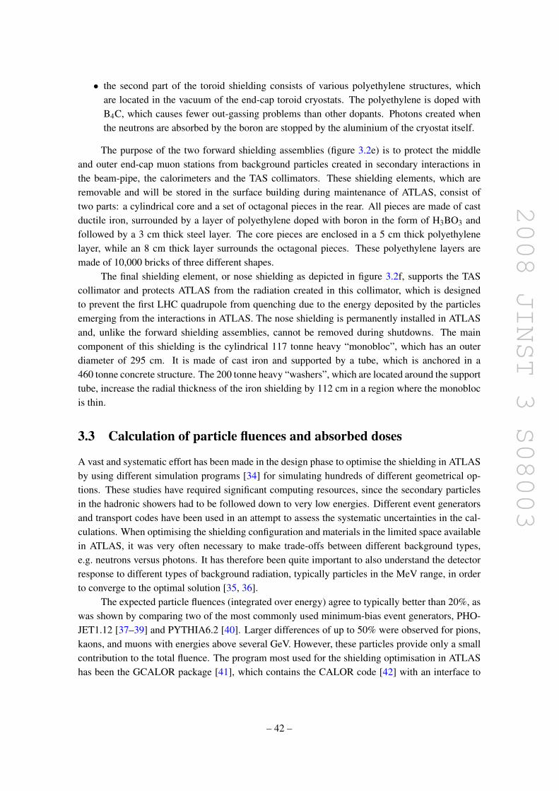
2008 JINST 3 S08003

• the second part of the toroid shielding consists of various polyethylene structures, whichare located in the vacuum of the end-cap toroid cryostats. The polyethylene is doped withB4C, which causes fewer out-gassing problems than other dopants. Photons created whenthe neutrons are absorbed by the boron are stopped by the aluminium of the cryostat itself.

The purpose of the two forward shielding assemblies (figure 3.2e) is to protect the middleand outer end-cap muon stations from background particles created in secondary interactions inthe beam-pipe, the calorimeters and the TAS collimators. These shielding elements, which areremovable and will be stored in the surface building during maintenance of ATLAS, consist oftwo parts: a cylindrical core and a set of octagonal pieces in the rear. All pieces are made of castductile iron, surrounded by a layer of polyethylene doped with boron in the form of H3BO3 andfollowed by a 3 cm thick steel layer. The core pieces are enclosed in a 5 cm thick polyethylenelayer, while an 8 cm thick layer surrounds the octagonal pieces. These polyethylene layers aremade of 10,000 bricks of three different shapes.

The final shielding element, or nose shielding as depicted in figure 3.2f, supports the TAScollimator and protects ATLAS from the radiation created in this collimator, which is designedto prevent the first LHC quadrupole from quenching due to the energy deposited by the particlesemerging from the interactions in ATLAS. The nose shielding is permanently installed in ATLASand, unlike the forward shielding assemblies, cannot be removed during shutdowns. The maincomponent of this shielding is the cylindrical 117 tonne heavy “monobloc”, which has an outerdiameter of 295 cm. It is made of cast iron and supported by a tube, which is anchored in a460 tonne concrete structure. The 200 tonne heavy “washers”, which are located around the supporttube, increase the radial thickness of the iron shielding by 112 cm in a region where the monoblocis thin.

3.3 Calculation of particle fluences and absorbed doses

A vast and systematic effort has been made in the design phase to optimise the shielding in ATLASby using different simulation programs [34] for simulating hundreds of different geometrical op-tions. These studies have required significant computing resources, since the secondary particlesin the hadronic showers had to be followed down to very low energies. Different event generatorsand transport codes have been used in an attempt to assess the systematic uncertainties in the cal-culations. When optimising the shielding configuration and materials in the limited space availablein ATLAS, it was very often necessary to make trade-offs between different background types,e.g. neutrons versus photons. It has therefore been quite important to also understand the detectorresponse to different types of background radiation, typically particles in the MeV range, in orderto converge to the optimal solution [35, 36].

The expected particle fluences (integrated over energy) agree to typically better than 20%, aswas shown by comparing two of the most commonly used minimum-bias event generators, PHO-JET1.12 [37–39] and PYTHIA6.2 [40]. Larger differences of up to 50% were observed for pions,kaons, and muons with energies above several GeV. However, these particles provide only a smallcontribution to the total fluence. The program most used for the shielding optimisation in ATLAShas been the GCALOR package [41], which contains the CALOR code [42] with an interface to

– 42 –

2008 JINST 3 S08003

GEANT3 [43]. FLUKA2001 [44] is another transport code, which is widely used for studies ofhadronic and electromagnetic cascades induced by high-energy particles, and which has been ex-tensively used in simulations of background radiation in ATLAS. In order to investigate transport-code differences, GCALOR was compared not only to FLUKA but also to MARS14(2002) [45].Comparisons for simplified geometries as well as for the most detailed descriptions of the detectorhave been carried out.

The results of these studies are extensively reported in [34]: the overall conclusion is that thepredictions of FLUKA, MARS and GCALOR are in good agreement for energy-integrated neutron,charged hadron, photon and e+e− fluences. For most regions in the inner detector, the differencebetween the FLUKA and GCALOR values is below 40%. In the pixel vertexing layer differencesas large as 80% are however observed for charged hadrons. An excellent agreement, typicallyto within 20%, between the respective photon and neutron fluences in the muon spectrometer isobserved when comparing the FLUKA and the GCALOR results. The charged hadron and leptonfluences in the muon spectrometer show much larger discrepancies, but the differences are alwayswithin a factor of 2.5. An overall safety factor of five has been used in the design of the ATLASmuon spectrometer.

The absorbed dose is the mean energy deposited per unit mass, taking into account all energy-loss mechanisms (but corrected for rest-mass effects). The dominant energy-loss mechanism isusually ionisation, but non-ionising energy loss is also important for understanding detector andelectronic damage effects. The ionising dose is defined in the following as the integrated dE/dxenergy loss in the detector material from charged particles, excluding ionisation energy loss fromnuclear recoils. It is given in units of Gy/y, where one year corresponds to 8× 1015 inelastic proton-proton collisions (assuming an inelastic cross-section of 80 mb, a luminosity of 1034 cm−2 s−1 anda data-taking period of 107 s). Comparisons of the calculated ionising dose in the inner detectorbetween FLUKA and GCALOR show differences of up to a factor of two.

3.3.1 The inner-detector and calorimeter regions

Figure 3.3 shows a GCALOR calculation of the ionising dose in the region closest to the interactionpoint. The forward calorimeters will be exposed to up to 160 kGy/y, whereas the correspondingnumber for the end-cap electromagnetic calorimeters is 30 kGy/y. This will lead to very largeintegrated doses over the full lifetime of the experiment and is one of the main reasons why only theLAr technology with its intrinsically high resistance to radiation is used in the end-cap and forwardregions. The main concern in the design phase has been for the electrode materials, primarilypolymers such as polyimide, which had to be chosen with care and thoroughly tested for radiationhardness [46, 47].

The tile calorimeter, with its scintillator samplings read out by wavelength-shifting fibres, isprotected by the LAr electromagnetic calorimeter and is exposed to less than 30 Gy/y, i.e. 5,000times less than the forward calorimeters. The scintillators and fibres were nevertheless also thor-oughly studied under irradiation [48–51] in order to determine their degradation during the lifetimeof ATLAS.

In the inner detector, a very large effort had to be devoted over many years to the understand-ing of the impact of irradiation on silicon sensors, on front-end electronics circuits and on ageingphenomena in the ionising gas used for the straw tubes.

– 43 –

2008 JINST 3 S08003

Gy/year

10

1

100

1000

10000 100000

Rad

ius (

m)

z (m)

T R T

S C T Pixels F C al

LAr barrelcalorimeter

Tilecalorimeter

Tilecalorimeter

LAr end-capcalorimeter CSC

MDT

Figure 3.3: The total ionising dose per year calculated by GCALOR (see text) in one quarter ofthe central part of the detector. The locations of the inner detector sub-systems, of the differentcalorimeters and of the inner end-cap muon stations are indicated. The scale on the left gives theintegrated dose per year corresponding to the various iso-lines.

Two main mechanisms lead to the degradation of the performance of silicon devices underirradiation. First, there is the effect of damage to the devices due to ionising energy loss. This canlead to the creation of trapped charges, in particular in the oxide layer of the sensor, which alters itselectric properties. The second effect is bulk damage, or displacement damage, which is caused bythe displacement of silicon atoms in the lattice. In the study of bulk damage to silicon devices, it isuseful to introduce a quantity called the 1 MeV neutron equivalent fluence (Fneq). This fluence isobtained by convoluting the various particle energy spectra and fluences with silicon displacement-damage functions, normalised using the non-ionising energy loss (NIEL) cross-sections to the ex-pected damage of 1 MeV neutrons [52].

Table 3.1 lists the particle rates, Fneq values and ionising doses predicted by FLUKA in theinner detector regions shown in figure 3.3. In the pixel detector, the particle rates are dominated bycharged pions and photons. The latter are produced mostly in neutron capture processes but alsodirectly from the primary collisions and from interactions in the beam-pipe and its related equip-ment. The predicted ionising dose in the innermost layer of the barrel pixel detector is 160 kGy/y,

– 44 –

2008 JINST 3 S08003

Table 3.1: Particle rates, fluences and doses in key locations of the inner detector sub-systems(see figure 4.2 for the definitions and positions of the inner detector layers). Here, Fneq is the1 MeV neutron equivalent fluence (see text). The FLUKA program has been used for this calcula-tion and the statistical uncertainties are typically less than 10%. One year corresponds to 8 × 1015

inelastic proton-proton collisions (assuming an inelastic cross-section of 80 mb, a luminosityof 1034 cm−2 s−1 and a data-taking period of 107 s).

Particle rates (kHz/cm2) Fneq Ionisation

Region R (cm) γ Protons Neutrons π± µ± e− (×10+12 cm−2) dose (Gy/y)

> 30 keV > 10 MeV > 100 keV > 10 MeV > 10 MeV > 0.5 MeV

Pixel layer 0 5.05 45800 2030 4140 34100 300 8140 270 158000

Pixel layer 2 12.25 9150 280 1240 4120 190 1730 46 25400

SCT barrel layer 1 29.9 4400 80 690 990 130 690 16 7590

SCT barrel layer 4 51.4 3910 36 490 370 67 320 9 2960

SCT end-cap disk 9 43.9 7580 73 840 550 110 470 14 4510

TRT outer radius 108.0 2430 10 380 61 7 53 5 680

which is the same as for the forward calorimeter, while the Fneq is expected to be 3 × 1014 cm−2/y.In the SCT detector, the charged hadron and neutron rates are comparable and the Fneq and theionising dose are reduced by about a factor of 20 with respect to the first pixel layer.

While most of the charged hadrons originate from the interaction point, most of the neutronsin the inner detector are the result of albedo (back-splash from the calorimeters). The purposeof the moderator shielding described in section 3.2 is to moderate the neutrons from the end-capand forward calorimeters to lower their energies to values for which their contribution to the totalFneq is minimised. The polyethylene in the moderator shielding is doped with boron, which has alarge cross-section for the capture of thermal neutrons. Nevertheless, the inner detector cavity willbe filled during LHC operation by an almost uniform “gas” of thermal neutrons with a flux of 1–2 MHz/cm2 and the sensitive detectors will be exposed to fluxes of 2–10 MHz/cm2 of low-energyphotons originating from the interactions themselves and from neutron capture. The dominantlong-term impact of these particle fluences is not only radiation damage but also activation of thedetector components (see section 3.5).

3.3.2 The muon spectrometer region

The effects of the absorbed ionising dose in the most critical muon spectrometer regions have beenstudied [53]. The CSC’s in the inner end-cap stations will be exposed to the highest dose. Figure 3.3shows that in this region the ionising dose will vary between 3 and 20 Gy/y. The chambers closestto the beam-line in the middle end-cap stations are expected to see at most 10 Gy/y. Most of themuon spectrometer will, however, be exposed to less than 1 Gy/y.

Although care had also to be applied to the choices of materials, to the design of the front-endelectronics circuits and to the choice of the ionising gases for all the muon chamber technologies,radiation damage due to the ionising dose is not the only concern in the muon spectrometer region.

– 45 –

2008 JINST 3 S08003

QUADTASFCal

Inner det.

Barrel middlemuons

Barrel outermuons

Barrel innermuons

End-cap middle

End-cap outer

muons muons

End-cap inner muons

End-cap toroid

Disk Toroid shield.

Forwardshielding

Noseshield.

n: 2.7J: 1.0P: 1.5p: 1.1

n: 3.1J: 1.1P: 2.4p: 2.3

n: 3.5J: 1.2P: 4.5p: 2.2

n: 2.6J: 1.0P: 0.4p: 0.9

n: 2.8J: 1.1P: 0.5p: 1.6

n: 3.8J: 1.4P: 0.8p: 3.2

n: 2.7J: 1.1P: 0.3p: 0.4

n: 3.4J: 1.3P: 0.4p: 1.0

n: 4.0J: 1.5P: 0.4p: 1.6

n: 79J: 25

P: 21p: 64

n: 34J: 11

P: 20p: 23

n: 17J: 5.4

P: 6.7p: 12

n: 7.7J: 2.4

P: 3.4p: 8.3

n: 3.1J: 11

P: 8.7 p: 11

n: 3.4J: 1.7P: 0.9p: 4.9

n: 4.0J: 4.4P: 3.0p: 10

n: 1.7J: 0.8P: 0.5p: 0.9

n: 2.0J: 1.2P: 1.2p: 1.4

n: 2.7J: 1.5P: 3.0p: 0.9

LAr cal.LAr cal.

Tile cal. Tile cal.

Figure 3.4: Particle fluxes in the various muon spectrometer stations at high luminosity(1034 cm−2 s−1) as predicted by GCALOR. The neutron and photon fluxes are in units of kHz/cm2

and the muon and proton fluxes in Hz/cm2.

Signals in the detectors from background particles are the main issue, because these backgroundsignals may significantly reduce the muon track-finding efficiency and, more importantly, introducelarge rates of fake triggers. The expected particle fluxes based on a simulation of the backgroundradiation in the ATLAS muon spectrometer using the GCALOR program are shown in figure 3.4.The energy thresholds used in these simulations are 10 keV, 10−11 MeV (well below the thermalneutron energy range), 1 MeV, and 1 MeV for photons, neutrons, muons, and protons, respectively.The highest fluxes are expected in the innermost end-cap muon stations, in particular in the CSC’s,which will have to cope with a large background counting rate, although the estimation of this rateis subject to systematic uncertainties between approximately 15% and 25%.

Background hit rates caused by neutrons and photons in the relevant energy range have beencalculated with GEANT3 for all muon-chamber technologies using detailed geometrical descrip-tions of the muon chamber setup. Energy-dependent efficiency curves have been estimated forneutrons, photons, and electrons [34]. Calculations have been done for the various chamber typestaking into account the angular distributions of the particles at the chamber locations. Fluxes tendto be isotropic in the barrel, while in the end-cap a substantial fraction of the particles originatesfrom the interaction region and from the beam-pipe in the region of the end-cap toroids, whichis the main local source of secondary radiation. The fake L1 trigger rate in the presence of thesebackground hits was studied in simulation including large contingency factors to account for thevarious uncertainties in the predictions.

– 46 –

2008 JINST 3 S08003

8 9 13

8 10 12

MDT: 6

MDT: 9

MDT: 12

MDT: 13TGC: 17

MDT: 68TGC: 66

MDT: 32TGC: 32

MDT: 23

MDT: 40

CSC: 347

TASFCal Disk

MDT: 103TGC: 100

End-cap middle

End-cap outer

Noseshield.

Forwardshielding

muons muons

Barrel middlemuons

Barrel outermuons

Barrel innermuons

RPC:

RPC:

Toroid shield.QUAD

End-cap toroid

7 9 10MDT:

6 8 11MDT:

8 10 11MDT:

End-cap inner muons

Tile cal. Tile cal.

LAr cal.LAr cal.

Inner det.

Figure 3.5: Average expected single-plane counting rates in Hz/cm2 at 1034 cm−2 s−1 and forvarious regions in the muon spectrometer.

The single-plane efficiency curves have been compared between existing experimental dataand simulation and found to be in good agreement. Average single-plane chamber efficiencieshave been obtained by folding efficiency curves with the energy spectra predicted at each chamberlocation. Uncertainties due to the shape of the energy spectrum, the angular distribution, and thesurrounding material have been studied and amount to a factor of 1.5. Predicted counting ratesin the barrel stations are of the order of 10–12 Hz/cm2 for both the MDT’s and the resistive platechambers. These rates are dominated by the photon contribution (80%), followed by neutrons andprotons (10% each). In the inner barrel stations, the contribution from muons rises to about 15%and that from punch-through pions to a few percent. In the end-cap regions, photons contributeless to the counting rate. In the CSC’s for example, photons account for about half of the rate,while muons account for 30% and protons for 10%. The predicted single-plane counting rates inthe muon spectrometer are summarised in figure 3.5.

3.4 Background monitors

Measurements of particle fluences in ATLAS will provide a precise bench-marking of the particletransport codes used in the calculations and will also directly monitor the absorbed doses in thevarious detectors. Possible beam losses near the detector have to be monitored with specific de-tectors designed to provide fast feedback to the accelerator operations team. The motivation forequipping ATLAS with a reliable set of background monitors in various regions of the detector istherefore obvious.

– 47 –

2008 JINST 3 S08003

3.4.1 Monitors in the inner detector

The inner detector region of ATLAS contains a set of small detectors, which are sensitive to dose,to the 1 MeV neutron equivalent fluence (Fneq) and to thermal neutrons. These detectors consist of:

1. Field-effect transistors (RADFET’s), which measure the total ionising dose;

2. PIN-diodes, which measure Fneq;

3. Radiation-hardened transistors, which measure thermal neutron fluences.

These detectors will measure the integrated doses and fluences in the inner detector and will alsoto some extent provide bench-marking estimates of the different contributions (charged particles,neutrons and photons).

One of the worst-case scenarios during LHC operation arises if several proton bunches hitthe collimators in front of the detectors. While the accumulated radiation dose from such unlikelyaccidents corresponds to that acquired during a few days of normal operation, and as such providesno major contribution to the integrated dose, the enormous instantaneous rate might cause detectordamage. The ATLAS Beam Conditions Monitor (BCM) [54] system consists of a set of detectorsdesigned to detect such incidents and trigger an abort in time to prevent serious damage to thedetector (see also section 9.10). These incidents need to be distinguished from the stray protonsand beam-gas backgrounds which frequently initiate charged particle showers, which originate wellupstream (or downstream) from the ATLAS interaction point. Due to their very fast response timeand intrinsically very high resistance to radiation, the BCM detectors will be used throughout thelifetime of the experiment to distinguish these stray beam particles from those originating fromproton-proton interactions.

The BCM system, designed to tolerate doses of up to 500 kGy and in excess of 1015 chargedparticles per cm2 over the lifetime of the experiment, consists of two stations, each with fourmodules. Each module, as depicted in figure 3.6 (left), includes two radiation-hard diamond sen-sors [55, 56] read out in parallel by radiation-tolerant electronics with a 1 ns rise-time [57]. Fig-ure 3.6 (right) shows a close-up view of one station installed around the beryllium beam-pipe. Thestations are located symmetrically around the interaction point at z = ±184 cm and R = 5.5 cm,which corresponds to a |η | = 4.2. The difference in time-of-flight between the two stations, ∆t,distinguishes particles from normal collisions (∆ t = 0, 25, 50 ns, etc.) from those arising fromstray protons (∆ t = 12.5, 37.5 ns, etc.). The in-time and out-of-time multi-module coincidencesare determined by an FPGA-based back-end, which digitises the signals, monitors the detector per-formance and generates beam-abort signals if warranted. Preliminary analysis of data on one of themodules in a high-energy pion test-beam shows a signal-to-noise ratio of 11 ± 2 in an operationalgeometry, where minimum ionising particles are incident on the BCM sensors at a 45 angle. Afull description of the design, construction and test-beam characterisation of the BCM system canbe found in [54].

3.4.2 Monitors in the muon spectrometer

Several sets of detectors have been installed in the end-cap muon stations to monitor the backgroundfluences and thus to constrain further the particle transport codes used in the calculations described

– 48 –

2008 JINST 3 S08003

Figure 3.6: Left: top view of a BCM module, showing the diamond sensors (left side of picture),the HV supply and signal-transmission lines, the two amplification stages and the signal connector(right side of picture). Right: close-up view of one BCM station installed at 184 cm from the centreof the pixel detector, which can be seen at the far end of the picture. Each one of the four modulescan be seen in position at a radius of 5.5 cm, very close to the beam-pipe.

in section 3.3. These detectors are installed inthe inner, middle, and outer end-cap stations.

Scintillation detectors

Ionisation chamber Proportional tube

Figure 3.7: Picture of one set of backgroundmonitors, to be installed in the thin gap chamberlayer of the middle end-cap muon station. Theeight different types of detectors are described inthe text.

Figure 3.7 shows one set of the detectors whichhave been installed. They were chosen to pro-vide a reliable response to neutrons or photonsin various energy ranges:

1. Boron-lined proportional tubes operat-ing with Ar/CO2 gas are used to mea-sure thermal and slow neutrons (ener-gies below 10−5 MeV). Each interactionn + 10B → Li + α sends a slow Li or α-particle into the tube. The large ionisa-tion pulse associated with the Li or α-particle is used for pulse-height discrim-ination against Compton electrons andminimum-ionising particles. These detec-tors are therefore relatively insensitive tophotons and charged particles.

2. Boron-loaded plastic scintillator (BC-454) is sensitive to the neutron interactions describedabove and is also used to study thermal and slow neutrons.

3. Detectors with a plastic disk loaded with LiF and coated with a thin layer of ZnS(Ag) scin-tillator are sensitive to the tritium and α-particles produced in the neutron capture process inlithium.

– 49 –

2008 JINST 3 S08003

4. Another ZnS(Ag) scintillator embedded in plastic is used to study fast neutrons (with ener-gies of a few MeV). The plastic is rich in hydrogen, from which incoming neutrons scat-ter to produce recoil protons. These protons produce large ionisation pulses compared tominimum-ionising particles or low-energy electrons. Pulse-height discrimination schemesshould therefore provide good rejection against these backgrounds.

5. A liquid scintillator, with pulse-shape discrimination electronics, is used in combination withplastics to measure fast neutrons.

6. Scintillator detectors with NaI and lutetium oxyorthosilicate (LSO) crystals are used to mea-sure the low-energy photon spectrum (0 to 10 MeV). The spectrum is dominated by photons,but also contains a neutron component, which can be separated out using fitting techniquesand detailed simulations.

7. Small ionisation chambers measure the total ionising dose.

3.4.3 Network of detectors for radiation measurements

A system of small silicon pixel detectors has been developed for radiation measurements in theexperimental environment [58, 59]. This detector network will form a stand-alone system fully ca-pable of delivering real-time images of fluxes and spectral composition of different particle species,including slow and fast neutrons.

These silicon detectors will be operated via active USB cables and USB-ethernet extendersby a PC placed in the underground USA15 counting room, located next to the main cavern. Thehybrid silicon pixel device consists of a silicon detector chip, 300 µm thick with 256×256 pixels,bonded to a readout chip. Each of the 55 µm×55 µm pixels is connected to its respective readoutchain integrated on the chip. Settings of the pulse height discriminators determine the input energywindow and at the same time provide noise suppression. The pixel counter determines the numberof interacting quanta of radiation falling within this window. These devices can be used for positionand energy sensitive (from 5 keV up to tens of MeV) spectroscopic detection of radiation. Theyare also capable of counting particle fluxes at rates in excess of GHz/cm2.

This system can be used in both tracking and counting modes, to record tracks or countscaused by x-rays, gamma-radiation, neutrons, electrons, minimum ionising particles and ions.For neutron detection, the silicon detectors are partially covered by neutron converters (6LiF andpolyethylene for slow and fast neutrons, respectively). The tracking mode is based on electronicvisualisation of tracks and traces of individual quanta of radiation in the sensitive silicon volume.In the case of count rates above 5× 103 events/cm2 s, the devices are operated in counting mode,in which charge deposition in the pixels is counted at different threshold settings. Calibration ofthe devices enables the conversion of the individual tracks observed and/or counts measured intofluxes of respective types of radiation and dose rates. At least 14 of these pixel devices will beplaced inside ATLAS: four devices on the LAr calorimeter facing the inner detector, four deviceson the tile calorimeter, four devices near the muon chambers in the inner end-cap muon station,and two devices near the forward shielding and close to the outer end-cap muon station.

– 50 –

2008 JINST 3 S08003

3.5 Activation

Induced radioactivity will be a major problem at the LHC, and ATLAS is the experiment with thehighest levels of induced radiation. This is due to the small radius of the ATLAS beam-pipe, thesmall bore of the forward calorimeters, and to the shielding elements close to the beam-pipe. Acomprehensive study has been made of the expected activation in different regions and for differentdata-taking and cooling-off scenarios. The methods and assumptions used in the calculation of theinduced activity are given in [34]. The main conclusion of these studies is that the beam-pipe willbe the major source of induced radioactivity in ATLAS.

Three different access scenarios are foreseen for ATLAS during shutdowns, as described inmore detail in section 9.7. They are described below and two of the scenarios are depicted infigures 3.8 and 3.9.

(a) In the very short access scenario, all detector components remain in place and the magneticfields remain on. These accesses are typically on the order of a few hours long.

(b) In the short access scenario, the beam-pipe remains in place, but then acts as a linear sourceof photon radiation as can be seen in figure 3.8. Because of the high level of radiation, thearea around the beam-pipe, out to a radius of about 1 m, has to be fenced off after high-luminosity running. This will ensure that people working in ATLAS during short accesswill not be exposed to dose rates larger than 0.1 mSv/h (maintenance work in ATLAS will bedesigned to limit the yearly dose to 6 mSv per person). The only detector which is truly insidethe barrier is the inner detector. During a short access, maintenance of the inner detector willtherefore be severely limited.

(c) In the long access scenario, all the beam-pipe sections except the one inside the inner detectorvolume are removed as well as the small muon wheel (or inner end-cap muon stations)and the end-cap toroids. Two hot spots can clearly be seen in the final configuration, asshown in figure 3.9. One is the end-piece of the inner detector beam-pipe, which is madeof aluminium, whereas the rest of the inner detector beam-pipe is made of beryllium. Theexpected dose rate can reach 0.2 mSv/h at this location. The other hot spot is in front ofthe forward calorimeters, where the dose rate is predicted to reach very high values of upto 0.5 mSv/h. These relatively small-size regions will therefore be temporarily shielded withlead blocks during maintenance of the inner detector.

While the beam-pipe section inside the inner detector is mostly made of beryllium, the restof the beam-pipe is made of stainless steel and has to be removed in the case of the long accessscenario, since it will become very radioactive with a contact dose rate of 3–5 mSv/h. This could incertain cases inflict several mSv of integrated dose to personnel performing the intervention. Oneway of reducing the dose to personnel would be to make the beam-pipe out of aluminium instead ofstainless steel. This is expected to give a factor 10–50 reduction of the dose levels. If the beam-pipematerial were instead to be changed to beryllium over the whole length of the detector, the doserate would decrease by a factor of 100–1000 and would no longer be a problem. This is, however,very costly and will only be discussed further in the context of the LHC upgrade programme.

– 51 –

2008 JINST 3 S08003

QUADTAS

ToroidMuons

100-2000

50-100

10-50PSv/h

Rails

PSv/h

PSv/hxxxxxxxxxxxxxxxxxxxxxxxxxxxxxxxxxxxxxxxxxxxxxxxx

xxxxxxxxxxxxxxxxxxxxxxxxxxxxxxxxxxxxxxxxxxxxxxxxxxxxxxxxxxxxxxxxxxxxxxxxxxxxxxxxxxxxxxxxxxxxxxxxxxxxxxxxxxxxxxxxxxxxxxxxxxxxxxxxxxxxxxxxxxxxxxxxxxxxxxxxxxxxxxxxxxxxxxxxxxxxxxxxxxxxxxxxxxxxxxxxxxxxxxxxxxxxxxxxxxxxxxxxxxxxxxxxxxxxxxxxxxxxxxxxxxxxxxxxxxxxxxxxxxxxxxxxxxxxxxxxxxxxxxxxxxxxxxxxxxxxxxxxxxxxxxxxxxxxxxxxxxxxxxxxxxxxxxxxxxxxxxxxxxxxxxxxxxxxxxxxxxxxxxxxxxxxxxxxxxxxxxxxxxxxxxxxxxxxxxxxxxxxxxxxxxxxxxxxxxxxxxxxxxxxxxxxxxxxxxxxxxxxxxxxxxxxxxxxxxxxxxxxxxxxxxxxxxxxxxxxxxxxxxxx

xxxxxxxxxxxxxxxxxxxxxxxxxxxxxxxxxxxxxxxxxxxxxxxxxxxxxxxxxxxxxxxxxxxxxxxxxxxxxxxxxxxxxxxxxxxxxxxxxxxxxxxxxxxxxxxxxxxxxxxxxxxxxxxxxxxxxxxxxxxxxxxxxxxxxxxxxxxxxxxxxxxxxxxxxxxxxxxxxxxxxxxxxxxxxxxxxxxxxxxxxxxxxxxxxxxxxxxxxxxxxxxxxxxxxxxxxxxxxxxxxxxxxxxxxxxxxxxxxxxxxxxxxxxxxxxxxxxxxxxxxxxxxxxxxxxxxxxxxxxxxxxxxxxxxxxxxxxxxxxxxxxxxxxxxxxxxxxxxxxxxxxxxxxxxxxxxxxxxxxxxxxxxxxxxxxxxxxxxxxxxxxxxxxxxxxxxxxxxxxxxxxxxxxxxxxxxxxxxxxxxxxxxxxxxxxxxxxxxxxxxxxxxxxxxxxxxxxxxxxxxxxxxxxxxxxxxxxxxxxxxxxxxxxxxxxxxxxxxxxxxxxxxxxxxxxxxxxxxxxxxxxxxxxxxxxxxxxxxxxxxxxxxxxxxxxxxxxxxxxxxxxxxxxxxxxxxxxxxxxxxxxxxxxxxxxxxxxxxxxxxxxxxxxxxxxxxxxxxxxxxxxxxxxxxxxxxxxxxxxxxxxxxxxxxxxxxxxxxxxxxxxxxxxxxxxxxxxxxxxxxxxxxxxxxxxxxxxxxxxxxxxxxxxxxxxxxxxxxxxxxxxxxxxxxxxxxxxxxxxxxxxxxxxxxxxxxxxxxxxxxxxxxxxxxxxxxxxxxxxxxxxxxxxxxxxxxxxxxxxxxxxxxxxxxxxxxxxxxxxxxxxxxxxxxxxxxxxxxxxxxxxxxxxxxxxxxxxxxxxxxxxxxxxxxxxxxxxxxxxxxx

xxxxxxxxxxxxxxxxxxxxxxxxxxxxxxxxxxxxxxxxxxxxxxxxxxxxxxxxxxxxxxxxxxxxxxxxxxxxxxxxxxxxxxxxxxxxxxxxxxxxxxxxxxxxxxxxxxxxxxxxxxxxxxxxxxxxxxxxxxxxxxxxxxxxxxxxxxxxxxxxxxxxxxxxxxxxxxxxxxxxxxxxxxxxxxxxxxxxxxxxxxxxxxxxxxxxxxxxxxxxxxxxxxxxxxxxxxxxxxxxxxxxxxxxxxxxxxxxxxxxxxxxxxxxxxxxxxxxxxxxxxxxxxxxxxxxxxxxxxxxxxxxxxxxxxxxxxxxxxxxxxxxxxxxxxxxxxxxxxxxxxxxxxxxxxxxxxxxxxxxxxxxxxxxxxxxxxxxxxxxxxxxxxxxxxxxxxxxxxxxxxxxxxxxxxxxxxxxxxxxxxxxxxxxxxxxxxxxxxxxxxxxxxxxxxxxxxxxxxxxxxxxxxxxxxxxxxxxxxxxxxxxxxxxxxxxxxxxxxxxxxxxxxxxxxxxxxxxxxxxxxxxxxxxxxxxxxxxxxxxxxxxxxxxxxxxxxxxxxxxxxxxxxxxxxxxxxxxxxxxxxxxxxxxxxxxxxxxxxxxxxxxxxxxxxxxxxxxxxxxxxxxxxxxxxxxxxxxxxxxxxxxxxxxxxxxxxxxxxxxxxxxxxxxxxxxxxxxxxxxxxxxxxxxxxxxxxxxxxxxxxxxxxxxxxxxxxxxxxxxxxxxxxxxxxxxxxxxxxxxxxxxxxxxxxxxxxxxxxxxxxxxxxxxxxxxxxxxxxxxxxxxxxxxxxxxxxxxxxxxxxxxxxxxxxxxxxxxxxxxxxxxxxxxxxxxx

xxxxxxxxxxxxxxxxxxxxxxxxxxxxxxxxxxxxxxxxxxxxxxxxxxxxxxxxxxxxxxxxxxxxxxxxxxxxxxxxxxxxxxxxxxxxxxxxxxxxxxxxxxxxxxxxxxxxxxxxxxxxxxxxxxxxxxxxxxxxxxxxxxxxxxxxxxxxxxxxxxxxxxxxxxxxxxxxxxxxxxxxxxxxxxxxxxxxxxxxxxxxxxxxxxxxxxxxxxxxxxxxxxxxxxxxxxxxxxxxxxxxxxxxxxxxxxxxxxxxxxxxxxxxxxxxxxxxxxxxxxxxxxxxxxxxxxxxxxxxxxxxxxxxxxxxxxxxxxxxxxxxxxxxxxxxxxxxxxxxxxxxxxxxxxxxxxxxxxxxxxxxxxxxxxxxxxxxxxxxxxxxxxxxxxxxxxxxxxxxxxxxxxxxxxxxxxxxxxxxxxxxxxxxxxxxxxxxxxxxxxxxxxxxxxxxxxxxxxxxxxxxxxxxxxxxxxxxxxxxxxxxxxxxxxxxxxxxxxxxxxxxxxxxxxxxxxxxxxxxxxxxxxxxxxxxxxxxxxxxxxxxxxxxxxxxxxxxxxxxxxxx

xxxxxxxxxxxxxxxxxxxxxxxxxxxxxxxxxxxxxxxxxxxxxxxxxxxxxxxxxxxxxxxxxxxxxxxxxxxxxxxxxxxxxxxxxxxxxxxxxxxxxxxxxxxxxxxxxxxxxxxxxxxxxxxxxxxxxxxxxxxxxxxxxxxxxxxxxxxxxxxxxxxxxxxxxxxxxxxxxxxxxxxxxxxxxxxxxxxxxxxxxxxxxxxxxxxxxxxxxxxxxxxxxxxxxxxxxxxxxxxxxxxxxxxxxxxxxxxxxxxxxxxxxxxxxxxxxxxxxxxxxxxxxxxxxxxxxxxxxxxxxxxxxxxxxxxxxxxxxxxxxxxxxxxxxxxxxxxxxxxxxxxxxxxxxxxxxxxxxxxxxxxxxxxxxxxxxxxxxxxxxxxxxxxxxxxxxxxxxxxxxxxxxxxxxxxxxxxxxxxxxxxxxxxxxxxxxxxxxxxxxxxxxxxxxxxxxxxxxxxxxxxxxxxxxxxxxxxxxxxxxxxxxxxxxxxxxxxxxxxxxxxxxxxxxxxxxxxxxxxxxxxxxxxxxxxxxxxxxxxxxxxxxxxxxxxxxxxxxxxxxxxxxxxxxxxxxxxxxxxxxxxxxxxxxxxxxxxxxxxxxxxxxxxxxxxxxxxxxxxxxxxxxxxxxxxxxxxxxxxxxxxxxxxxxxxxxxxxxxxxxxxxxxxxxxxxxxxxxxxxxxxxxxxxxxxxxxxxxxxxxxxxxxxxxxxxxxxxxxxxxxxxxxxxxxxxxxxxxxxxxxxxxxxxxxxxxxxxxxxxxxxxxxxxxxxxxxxxxxxxxxxxxxxxxxxxxxxxxxxxxxxxxxxxxxxxxxxxxxxxxxxxxxxxxxxxx

xxxxxxxxxxxxxxxxxxxxxxxxxxxxxxxxxxxxxxxxxxxxxxxxxxxxxxxxxxxxxxxxxxxxxxxxxxxxxxxxxxxxxxxxxxxxxxxxxxxxxxxxxxxxxxxxxxxxxxxxxxxxxxxxxxxxxxxxxxxxxxxxxxxxxxxxxxxxxxxxxxxxxxxxxxxxxxxxxxxxxxxxxxxxxxxxxxxxxxxxxxxxxxxxxxxxxxxxxxxxxxxxxxxxxxxxxxxxxxxxxxxxxxxxxxxxxxxxxxxxxxxxxxxxxxxxxxxxxxxxxxxxxxxxxxxxxxxxxxxxxxxxxxxxxxxxxxxxxxxxxxxxxxxxxxxxxxxxxxxxxxxxxxxxxxxxxxxxxxxxxxxxxxxxxxxxxxxxxxxxxxxxxxxxxxxxxxxxxxxxxxxxxxxxxxxxxxxxxxxxxxxxxxxxxxxxxxxxxxxxxxxxxxxxxxxxxxxxxxxxxxxxxxxxxxxxxxxxxxxxxxxxxxxxxxxxxxxxxxxxxxxxxxxxxxxxxxxxxxxxxxxxxxxxxxxxxxxxxxxxxxxxxxxxxxxxxxxxxxxxxxxxxxxxxxxxxxxxxxxxxxxxxxxxxxxxxxxxxxxxxxxxxxxxxxxxxxxxxxxxxxxxxxxxxxxxxxxxxxxxxxxxxxxxxxxxxxxxxxxxxxxxxxxxxxxxxxxxxxxxxxxxxxxxxxxxxxxxxxxxxxxxxxxxxxxxxxxxxxxxxxxxxxxxxxxxxxxxxxxxxxxxxxxxxxxxxxxxxxxxxxxxxxxxxxxxxxxxxxxxxxxxxxxxxxxxxxxxxxxxxxxxxxxxxxxxxxxxxxxxxxxxxxxxxxxxxxxxxxxxxxxxxxxxxxxxxxxxxxxxxxxxxxxxxxxxxxxxxxxxxxxxxxxxxxxxxxxxxxxx

Inner detector

shielding

Noseshield.

OuterMuons

MiddleMuons

Standard access

Barrel toroid coil

Tile cal. Tile cal.

LAr cal.LAr cal.

End-cap

End-cap End-cap

PSv/h

ToroidFCal

Short accessmiddlemuons

End-capoutermuons

End-cap

End-cap toroid

Figure 3.8: The inner region of the detector during one of the short access scenarios. The predicteddose rates have been calculated for 10 years of operation at 1034 cm−2 s−1 and for five days ofcooling off. The short access scenario (a) has the beam-pipe in place.

FCalQUADTAS

Outer

Rails

xxxxxxxxxxxxxxxxxxxxxxxxxxxxxxxxxxxxxxxxxxxxxxxxxxxxxxxxxxxxxxxxxxxxxxxxxxxxxxxxxxxxxxxxxxxxxxxxxxxxxxxxxxxxxxxxxxxxxxxxxxxxxxxxxxxxxxxxxxxxxxxxxxxxxxxxxxxxxxxxxxxxxxxxxxxxxxxxxxxxxxxxxxxxxxxxxxxxxxxxxxxxxxxxxxxxxxxxxxxxxxxxxxxxxxxxxxxxxxxxxxxxxxxxxxxxxxxxxxxxxxxxxxxxxxxxxxxxxxxxxxxxxxxxxxxxxxxxxxxxxxxxxxxxxxxxxxxxxxxxxxxxxxxxxxxxxxxxxxxxxxxxxxxxxxxxxxxxxxxxxxxxxxxxxxxxxxxxxxxxxxxxxxxxxxxxxxxxxxxxxxxxxxxxxxxxxxxxxxxxxxxxxxxxxxxxxxxxxxxxxxxxxxxxxxxxxxxxxxxxxxxxxxxxxxxxxxxxxxxxxxxxxxxxxxxxxxxxxxxxxxxxxxxxxxxxxxxxxxxxxxxxxxxx

xxxxxxxxxxxxxxxxxxxxxxxxxxxxxxxxxxxxxxxxxxxxxxxxxxxxxxxxxxxxxxxxxxxxxxxxxxxxxxxxxxxxxxxxxxxxxxxxxxxxxxxxxxxxxxxxxxxxxxxxxxxxxxxxxxxxxxxxxxxxxxxxxxxxxxxxxxxxxxxxxxxxxxxxxxxxxxxxxxxxxxxxxxxxxxxxxxxxxxxxxxxxxxxxxxxxxxxxxxxxxxxxxxxxxxxxxxxxxxxxxxxxxxxxxxxxxxxxxxxxxxxxxxxxxxxxxxxxxxxxxxxxxxxxxxxxxxxxxxxxxxxxxxxxxxxxxxxxxxxxxxxxxxxxxxxxxxxxxxxxxxxxxxxxxxxxxxxxxxxxxxxxxxxxxxxxxxxxxxxxxxxxxxxxxxxxxxxxxxxxxxxxxxxxxxxxxxxxxxxxxxxxxxxxxxxxxxxxxxxxxxxxxxxxxxxxxxxxxxxxxxxxxxxxxxxxxxxxxxxxxxxxxxxxxxxxxxxxxxxxxxxxxxxxxxxxxxxxxxxxxxxxxxxxxxxxxxxxxxxxxxxxxxxxxxxxxxxxxxxxxxxxxxxxxxxxxxxxxxxxxxxxxxxxxxxxxxxxxxxxxxxxxxxxxxxxxxxxxxxxxxxxxxxxxxxxxxxxxxxxxxxxxxxxxxxxxxxxxxxxxxxxxxxxxxxxxxxxxxxxxxxxxxxxxxxxxxxxxxxxxxxxxxxxxxxxxxxxxxxxxxxxxxxxxxxxxxxxxxxxxxxxxxxxxxxxxxxxxxxxxxxxxxxxxxxxxxxxxxxxxxxxxxxxxxxxxxxxxxxxxxxxxxxxxxxxxxxxxxxxxxxxxxxxxxxxxxxxxxxxxxxxxxxxxxxxxxxxxxxxxxxxxxxxxxxxxxxxxxxxxx

xxxxxxxxxxxxxxxxxxxxxxxxxxxxxxxxxxxxxxxxxxxxxxxxxxxxxxxxxxxxxxxxxxxxxxxxxxxxxxxxxxxxxxxxxxxxxxxxxxxxxxxxxxxxxxxxxxxxxxxxxxxxxxxxxxxxxxxxxxxxxxxxxxxxxxxxxxxxxxxxxxxxxxxxxxxxxxxxxxxxxxxxxxxxxxxxxxxxxxxxxxxxxxxxxxxxxxxxxxxxxxxxxxxxxxxxxxxxxxxxxxxxxxxxxxxxxxxxxxxxxxxxxxxxxxxxxxxxxxxxxxxxxxxxxxxxxxxxxxxxxxxxxxxxxxxxxxxxxxxxxxxxxxxxxxxxxxxxxxxxxxxxxxxxxxxxxxxxxxxxxxxxxxxxxxxxxxxxxxxxxxxxxxxxxxxxxxxxxxxxxxxxxxxxxxxxxxxxxxxxxxxxxxxxxxxxxxxxxxxxxxxxxxxxxxxxxxxxxxxxxxxxxxxxxxxxxxxxxxxxxxxxxxxxxxxxxxxxxxxxxxxxxxxxxxxxxxxxxxxxxxxxxxxxxxxxxxxxxxxxxxxxxxxxxxxxxxxxxxxxxxxxxxxxxxxxxxxxxxxxxxxxxxxxxxxxxxxxxxxxxxxxxxxxxxxxxxxxxxxxxxxxxxxxxxxxxxxxxxxxxxxxxxxxxxxxxxxxxxxxxxxxxxxxxxxxxxxxxxxxxxxxxxxxxxxxxxxxxxxxxxxxxxxxxxxxxxxxxxxxxxxxxxxxxxxxxxxxxxxxxxxxxxxxxxxxxxxxxxxxxxxxxxxxxxxxxxxxxxxxxxxxxxxxxxxxxxxxxxxxxxxxxxxxxxxxxxxxxxxxxxxxxxxxxxxxx

xxxxxxxxxxxxxxxxxxxxxxxxxxxxxxxxxxxxxxxxxxxxxxxxxxxxxxxxxxxxxxxxxxxxxxxxxxxxxxxxxxxxxxxxxxxxxxxxxxxxxxxxxxxxxxxxxxxxxxxxxxxxxxxxxxxxxxxxxxxxxxxxxxxxxxxxxxxxxxxxxxxxxxxxxxxxxxxxxxxxxxxxxxxxxxxxxxxxxxxxxxxxxxxxxxxxxxxxxxxxxxxxxxxxxxxxxxxxxxxxxxxxxxxxxxxxxxxxxxxxxxxxxxxxxxxxxxxxxxxxxxxxxxxxxxxxxxxxxxxxxxxxxxxxxxxxxxxxxxxxxxxxxxxxxxxxxxxxxxxxxxxxxxxxxxxxxxxxxxxxxxxxxxxxxxxxxxxxxxxxxxxxxxxxxxxxxxxxxxxxxxxxxxxxxxxxxxxxxxxxxxxxxxxxxxxxxxxxxxxxxxxxxxxxxxxxxxxxxxxxxxxxxxxxxxxxxxxxxxxxxxxxxxxxxxxxxxxxxxxxxxxxxxxxxxxxxxxxxxxxxxxxxxxxxxxxxxxxxxxxxxxxxxxxxxxxxxxxxxxxxxxx

xxxxxxxxxxxxxxxxxxxxxxxxxxxxxxxxxxxxxxxxxxxxxxxxxxxxxxxxxxxxxxxxxxxxxxxxxxxxxxxxxxxxxxxxxxxxxxxxxxxxxxxxxxxxxxxxxxxxxxxxxxxxxxxxxxxxxxxxxxxxxxxxxxxxxxxxxxxxxxxxxxxxxxxxxxxxxxxxxxxxxxxxxxxxxxxxxxxxxxxxxxxxxxxxxxxxxxxxxxxxxxxxxxxxxxxxxxxxxxxxxxxxxxxxxxxxxxxxxxxxxxxxxxxxxxxxxxxxxxxxxxxxxxxxxxxxxxxxxxxxxxxxxxxxxxxxxxxxxxxxxxxxxxxxxxxxxxxxxxxxxxxxxxxxxxxxxxxxxxxxxxxxxxxxxxxxxxxxxxxxxxxxxxxxxxxxxxxxxxxxxxxxxxxxxxxxxxxxxxxxxxxxxxxxxxxxxxxxxxxxxxxxxxxxxxxxxxxxxxxxxxxxxxxxxxxxxxxxxxxxxxxxxxxxxxxxxxxxxxxxxxxxxxxxxxxxxxxxxxxxxxxxxxxxxxxxxxxxxxxxxxxxxxxxxxxxxxxxxxxxxxxxxxxxxxxxxxxxxxxxxxxxxxxxxxxxxxxxxxxxxxxxxxxxxxxxxxxxxxxxxxxxxxxxxxxxxxxxxxxxxxxxxxxxxxxxxxxxxxxxxxxxxxxxxxxxxxxxxxxxxxxxxxxxxxxxxxxxxxxxxxxxxxxxxxxxxxxxxxxxxxxxxxxxxxxxxxxxxxxxxxxxxxxxxxxxxxxxxxxxxxxxxxxxxxxxxxxxxxxxxxxxxxxxxxxxxxxxxxxxxxxxxxxxxxxxxxxxxxxxxxxxxxxxxxxxx

xxxxxxxxxxxxxxxxxxxxxxxxxxxxxxxxxxxxxxxxxxxxxxxxxxxxxxxxxxxxxxxxxxxxxxxxxxxxxxxxxxxxxxxxxxxxxxxxxxxxxxxxxxxxxxxxxxxxxxxxxxxxxxxxxxxxxxxxxxxxxxxxxxxxxxxxxxxxxxxxxxxxxxxxxxxxxxxxxxxxxxxxxxxxxxxxxxxxxxxxxxxxxxxxxxxxxxxxxxxxxxxxxxxxxxxxxxxxxxxxxxxxxxxxxxxxxxxxxxxxxxxxxxxxxxxxxxxxxxxxxxxxxxxxxxxxxxxxxxxxxxxxxxxxxxxxxxxxxxxxxxxxxxxxxxxxxxxxxxxxxxxxxxxxxxxxxxxxxxxxxxxxxxxxxxxxxxxxxxxxxxxxxxxxxxxxxxxxxxxxxxxxxxxxxxxxxxxxxxxxxxxxxxxxxxxxxxxxxxxxxxxxxxxxxxxxxxxxxxxxxxxxxxxxxxxxxxxxxxxxxxxxxxxxxxxxxxxxxxxxxxxxxxxxxxxxxxxxxxxxxxxxxxxxxxxxxxxxxxxxxxxxxxxxxxxxxxxxxxxxxxxxxxxxxxxxxxxxxxxxxxxxxxxxxxxxxxxxxxxxxxxxxxxxxxxxxxxxxxxxxxxxxxxxxxxxxxxxxxxxxxxxxxxxxxxxxxxxxxxxxxxxxxxxxxxxxxxxxxxxxxxxxxxxxxxxxxxxxxxxxxxxxxxxxxxxxxxxxxxxxxxxxxxxxxxxxxxxxxxxxxxxxxxxxxxxxxxxxxxxxxxxxxxxxxxxxxxxxxxxxxxxxxxxxxxxxxxxxxxxxxxxxxxxxxxxxxxxxxxxxxxxxxxxxxxxxxxxxxxxxxxxxxxxxxxxxxxxxxxxxxxxxxxxxxxxxxxxxxxxxxxxxxxxxxxxxxxxxxxx

100-500 PSv/h

10-50 PSv/h

50-100 PSv/h

Inner detectorNose

shield.

MuonsMiddleMuonsBarrel toroid coil

Inner detector access

Tile cal. Tile cal.

LAr cal. LAr cal.

End-capEnd-cap

Long accessEnd-capmiddlemuons

End-capoutermuons

Figure 3.9: The inner region of the detector during one of the main long access scenarios. Thepredicted dose rates have been calculated for 10 years of operation at 1034 cm−2 s−1 and for fivedays of cooling off. The long access scenario (b) has only the inner detector section of the beam-pipe in place. The expected dose rates are greatly reduced in this access scenario.

– 52 –

2008 JINST 3 S08003

Chapter 4

Inner detector

4.1 Introduction

The ATLAS Inner Detector (ID) is designed to provide hermetic and robust pattern recognition,excellent momentum resolution and both primary and secondary vertex measurements [60, 61] forcharged tracks above a given pT threshold (nominally 0.5 GeV, but as low as 0.1 GeV in someongoing studies of initial measurements with minimum-bias events) and within the pseudorapidityrange |η | < 2.5. It also provides electron identification over |η | < 2.0 and a wide range of en-ergies (between 0.5 GeV and 150 GeV). This performance, which is required even at the highestluminosities expected from LHC collisions, is consequently at the limit of existing technology.

The ID layout, as shown in figure 4.1, reflects the performance requirements. The ID iscontained within a cylindrical envelope of length ±3512 mm and of radius 1150 mm, within asolenoidal magnetic field of 2 T (see section 2.2.4). Figures 4.2 and 4.3 show the sensors andstructural elements traversed by 10 GeV tracks in respectively the barrel and end-cap regions.

The ID consists of three independent but complementary sub-detectors. The envelopes ofeach sub-detector are listed in table 1.2 (see section 1.2) and shown in figure 4.1. At inner radii,high-resolution pattern recognition capabilities are available using discrete space-points from sili-con pixel layers and stereo pairs of silicon microstrip (SCT) layers. At larger radii, the transitionradiation tracker (TRT) comprises many layers of gaseous straw tube elements interleaved withtransition radiation material. With an average of 36 hits per track, it provides continuous track-ing to enhance the pattern recognition and improve the momentum resolution over |η | < 2.0 andelectron identification complementary to that of the calorimeter over a wide range of energies.

The high-radiation environment imposes stringent conditions on the inner-detector sensors,on-detector electronics, mechanical structure and services. Over the ten-year design lifetime of theexperiment, the pixel inner vertexing layer must be replaced after approximately three years of op-eration at design luminosity. The other pixel layers and the pixel disks must withstand a 1 MeV neu-tron equivalent fluence Fneq, defined in section 3.3.1 (see also [52]), of up to ∼8×1014cm−2. Theinnermost parts of the SCT must withstand Fneq of up to 2×1014cm−2. To maintain an adequatenoise performance after radiation damage, the silicon sensors must be kept at low temperature (ap-proximately −5 to −10C) implying coolant temperatures of ∼ –25C. In contrast, the TRT isdesigned to operate at room temperature.

– 53 –

2008 JINST 3 S08003

Envelopes

Pixel

SCT barrel

SCT end-cap

TRT barrel

TRT end-cap

255<R<549mm|Z|<805mm

251<R<610mm810<|Z|<2797mm

554<R<1082mm|Z|<780mm

617<R<1106mm827<|Z|<2744mm

45.5<R<242mm|Z|<3092mm

Cryostat

PPF1

CryostatSolenoid coil

z(mm)

Beam-pipe

Pixelsupport tubeSCT (end-cap)

TRT(end-cap)

1 2 3 4 5 6 7 8 9 10 11 12 1 2 3 4 5 6 7 8

Pixel

400.5495

580

650749

853.8934

1091.5

1299.9

1399.7

1771.4 2115.2 2505 2720.200

R50.5R88.5

R122.5

R299

R371

R443R514R563

R1066

R1150

R229

R560

R438.8R408

R337.6R275

R644

R1004

2710848712 PPB1

Radius(mm)

TRT(barrel)

SCT(barrel)Pixel PP1

3512ID end-plate

Pixel

400.5 495 580 6500

0

R50.5

R88.5

R122.5

R88.8

R149.6

R34.3

Figure 4.1: Plan view of a quarter-section of the ATLAS inner detector showing each of the majordetector elements with its active dimensions and envelopes. The labels PP1, PPB1 and PPF1indicate the patch-panels for the ID services.

The above operating specifications imply requirements on the alignment precision which aresummarised in table 4.1 and which serve as stringent upper limits on the silicon-module buildprecision, the TRT straw-tube position, and the measured module placement accuracy and stability.This leads to:

(a) a good build accuracy with radiation-tolerant materials having adequate detector stability andwell understood position reproducibility following repeated cycling between temperaturesof −20C and +20C, and a temperature uniformity on the structure and module mechanicswhich minimises thermal distortions;

(b) an ability to monitor the position of the detector elements using charged tracks and, for theSCT, laser interferometric monitoring [62];

(c) a trade-off between the low material budget needed for optimal performance and the sig-nificant material budget resulting from a stable mechanical structure with the services of ahighly granular detector.

The inner-detector performance requirements imply the need for a stability between alignmentperiods which is high compared with the alignment precision. Quantitatively, the track precisionshould not deteriorate by more than 20% between alignment periods.

– 54 –

2008 JINST 3 S08003

Figure 4.2: Drawing showing the sensors and structural elements traversed by a charged track of10 GeV pT in the barrel inner detector (η = 0.3). The track traverses successively the berylliumbeam-pipe, the three cylindrical silicon-pixel layers with individual sensor elements of 50×400µm2, the four cylindrical double layers (one axial and one with a stereo angle of 40 mrad) ofbarrel silicon-microstrip sensors (SCT) of pitch 80 µm, and approximately 36 axial straws of 4 mmdiameter contained in the barrel transition-radiation tracker modules within their support structure.

This chapter describes the construction and early performance of the as-built inner detector.In section 4.2, the basic detector sensor elements are described. Section 4.3 describes the detectormodules. Section 4.4 details the readout electronics of each sub-detector, section 4.5 describes thedetector power and control and section 4.6 describes the ID grounding and shielding. Section 4.7discusses the mechanical structure for each sub-detector, as well as the integration of the detectorsand their cooling and electrical services. The overall ID environmental conditions and generalservices are briefly summarised in section 4.8. Finally, section 4.9 indicates some initial results onthe operational performance and section 4.10 catalogues the material budget of the ID, which issignificantly larger than that of previous large-scale tracking detectors.

– 55 –

2008 JINST 3 S08003

Figure 4.3: Drawing showing the sensors and structural elements traversed by two charged tracksof 10 GeV pT in the end-cap inner detector (η = 1.4 and 2.2). The end-cap track at η = 1.4 traversessuccessively the beryllium beam-pipe, the three cylindrical silicon-pixel layers with individual sen-sor elements of 50×400 µm2, four of the disks with double layers (one radial and one with a stereoangle of 40 mrad) of end-cap silicon-microstrip sensors (SCT) of pitch ∼ 80 µm, and approxi-mately 40 straws of 4 mm diameter contained in the end-cap transition radiation tracker wheels.In contrast, the end-cap track at η = 2.2 traverses successively the beryllium beam-pipe, only thefirst of the cylindrical silicon-pixel layers, two end-cap pixel disks and the last four disks of theend-cap SCT. The coverage of the end-cap TRT does not extend beyond |η | = 2.

4.2 Inner-detector sensors

This section describes the detector sensors of the pixel, SCT and TRT sub-systems - silicon pixeland micro-strip sensors in section 4.2.1, and straw tubes filled with a Xe/CO2/O2 gas mixturein section 4.2.2. As discussed in section 3.3, the detector sensors are subject to large integratedradiation doses. They have therefore been developed and controlled to withstand the expectedirradiation, with a safety factor of approximately two.

4.2.1 Pixel and SCT detector sensors

The pixel and SCT sensors [63, 64] are required to maintain adequate signal performance overthe detector lifetime at design luminosity (with the exception of the pixel vertexing layer, as dis-cussed above). The integrated radiation dose has important consequences for the sensors of bothdetectors. In particular the required operating voltage, determined by the effective doping concen-tration, depends on both the irradiation and the subsequent temperature-sensitive annealing. Thesensor leakage current also increases linearly with the integrated radiation dose. The n-type bulkmaterial effectively becomes p-type after a fluence Fneq of ∼ 2×1013 cm−2. The effective dopingconcentration then grows with time in a temperature-dependent way. To contain this annealingand to reduce the leakage current, the sensors will, as noted above, be operated in the temperaturerange –5C to –10C. The sensors must further meet significant geometrical constraints on theirthickness, granularity and charge-collection efficiency.

– 56 –

2008 JINST 3 S08003

Table 4.1: Intrinsic measurement accuracies and mechanical alignment tolerances for the inner-detector sub-systems, as defined by the performance requirements of the ATLAS experiment. Thenumbers in the table correspond to the single-module accuracy for the pixels, to the effective single-module accuracy for the SCT and to the drift-time accuracy of a single straw for the TRT.

Item Intrinsic accuracy Alignment tolerances(µm) (µm)

Radial (R) Axial (z) Azimuth (R-φ)PixelLayer-0 10 (R-φ ) 115 (z) 10 20 7Layer-1 and -2 10 (R-φ ) 115 (z) 20 20 7Disks 10 (R-φ ) 115 (R) 20 100 7SCTBarrel 17 (R-φ ) 580 (z)1 100 50 12Disks 17 (R-φ ) 580 (R)1 50 200 12TRT 130 302

1Arises from the 40 mrad stereo angle between back-to-back sensors on the SCT modules

with axial (barrel) or radial (end-cap) alignment of one side of the structure. The result is

pitch-dependent for end-cap SCT modules.2The quoted alignment accuracy is related to the TRT drift-time accuracy.

The pixel sensors required the most leading-edge and novel technology to meet the verystringent specifications on radiation hardness, resolution and occupancy in the innermost layers.The sensors are 250 µm thick detectors, using oxygenated n-type wafers with readout pixels onthe n+-implanted side of the detector. Despite its higher cost and complexity, this novel designinvolving double-sided processing was used because:

(a) the n+ implants allow the detector to operate with good charge-collection efficiency aftertype inversion, even when operated below the depletion voltage, because the depletion zonegrows from the pixel side;

(b) highly oxygenated material has been shown to give increased radiation tolerance to chargedhadrons, with improved charge collection after type inversion and lower depletion voltage.

All of the 1744 pixel sensors (external dimensions 19×63 mm2) are identical. The sensorswill initially operate at∼ 150 V bias voltage, but operating voltages of up to 600 V will be requiredfor good charge collection efficiency after ten years of operation, depending on the sensor position,the integrated luminosity and the length of warm-up periods.The nominal pixel size is 50×400 µm2

(about 90% of the pixels) and is dictated by the readout pitch of the front-end electronics. The sizeof the remaining pixels is 50×600 µm2 in the regions at the front-end chips on a module. Thereare 47232 pixels on each sensor, but for reasons of space there are four ganged pixels in eachcolumn of the front-end chip, thus leading to a total of 46080 readout channels. A common bias

– 57 –

2008 JINST 3 S08003

Table 4.2: External cut dimensions of the SCT barrel and end-cap (EC) sensors. The tolerance onall external dimensions is ± 25 µm; the mask accuracy is at the level of ±1 µm. The inter-stripangle is that between adjacent strips of the sensor. The sensors are fabricated from 4-inch wafers.

Module type Sensor Cut length Outer width Inner width Strip pitch Inter-striptype (mm) (mm) (mm) (µm) angle (µrad)

Barrel Barrel 63.960 63.560 63.560 80.0 0

End-cap inner W12 61.060 55.488 45.735 56.9–69.2 207.0

End-cap middle W21 65.085 66.130 55.734 69.9–83.0 207.0

W22 54.435 74.847 66.152 83.4–94.2 207.0

End-cap outer W31 65.540 64.635 56.475 70.9–81.1 161.5

W32 57.515 71.814 64.653 81.5–90.4 161.5

grid ensures a DC connection to each pixel implant during wafer testing of sensor tiles, but it isonly AC-coupled in production modules due to concerns about the effects of high radiation doses.To guarantee optimal post-irradiation performance and to maintain a small feature size, a p-sprayisolation technology has been used [65]. Each pixel of a sensor is bump-bonded through a hole inthe passivation layer to an element of the front-end readout integrated circuit as part of the module.

For reasons of cost and reliability, the 15912 sensors of the SCT use a classic single-sidedp-in-n technology with AC-coupled readout strips. The sensors will initially operate at ∼ 150 Vbias voltage, but operating voltages of between 250 and 350 V will be required for good chargecollection efficiency after ten years of operation, depending on the sensor position, the integratedluminosity and the length of warm-up periods. The sensor thickness of 285±15 µm is a com-promise between the required operating voltage, the primary signal ionisation and the simplicityof fabrication. The strip pitch was determined by the required digitising precision, granularity,particle occupancy and noise performance. A strip pitch of 80 µm with two 6 cm-long sensorsdaisy-chained was chosen for the rectangular barrel sensors and radial strips of constant azimuthwith mean pitch of ∼ 80 µm were chosen for the trapezoidal end-cap sensors. There are thus atotal of 768 active strips of 12 cm length per sensor, plus two strips at bias potential to define thesensor edge. The detector dimensions are summarised in table 4.2 (see also table 4.7). Using thebinary readout electronics described in section 4.4, a noise occupancy per channel of < 5×10−4

for a threshold of 1 fC is specified for fully irradiated modules. The detectors were required tooperate stably at 500 V bias and to have < 1% of bad readout strips at 350 V bias before and afterirradiation to 3×1014 24 GeV protons/cm2, equivalent to the damage expected for a fluence Fneq

of 2×1014 cm−2.The SCT sensors were fabricated by two suppliers. For one supplier (7.8% of sensors), the p-

spray isolation technology causes difficulties of micro-discharges at low humidity. All sensors werecarefully tested, and a sub-sample was subjected to extended pixel or strip-by-strip studies [63, 64].A sub-sample was also used for extensive post-irradiation performance studies [63, 66–68]. Apartfrom precautions related to the humidity sensitivity noted above, the rejected strip sensors were atthe level of 1%. The pixel sensor rejection rate was somewhat higher because of a requirement tocarefully control the profile and doping concentration of the p-spray isolation.

– 58 –

2008 JINST 3 S08003

4.2.2 TRT straw tubes

Polyimide drift (straw) tubes of 4 mm diameter are the basic TRT detector elements [69]. The strawtube wall, especially developed to have good electrical and mechanical properties with minimalwall thickness, is made of two 35 µm thick multi-layer films bonded back-to-back. The barematerial, a 25 µm thick polyimide film, is coated on one side with a 0.2 µm Al layer which isprotected by a 5–6 µm thick graphite-polyimide layer. The other side of the film is coated by a5 µm polyurethane layer used to heat-seal the two films back-to-back. Mechanically, the straws arestabilised using carbon fibres. After fabrication, the straws were cut to length (144 cm for the barreland 37 cm for the end-caps) and leak-tested at 1 bar over-pressure. The straw (cathode) resistancewas required to be < 300 Ω/m.

For both the barrel and end-cap straws, the anodes are 31 µm diameter tungsten (99.95%)wires plated with 0.5–0.7 µm gold, supported at the straw end by an end-plug. They are directlyconnected to the front-end electronics (see section 4.4) and kept at ground potential. The anoderesistance is approximately 60 Ω/m and the assembled straw capacitance is < 10 pF. The signalattenuation length is∼ 4 m and the signal propagation time is∼ 4 ns/m. The cathodes are operatedtypically at –1530V to give a gain of 2.5×104 for the chosen gas mixture of 70% Xe, 27% CO2

and 3% O2 with 5−10 mbar over-pressure. A mixture containing 70% Ar and 30% CO2 has beenused during quality-control and cosmic-ray studies, resulting in an increased electron mobility anda degraded electron identification performance. Under normal operating conditions, the maximumelectron collection time is ∼ 48 ns and the operational drift-time accuracy is ∼ 130 µm [69]. Low-energy transition radiation (TR) photons are absorbed in the Xe-based gas mixture, and yield muchlarger signal amplitudes than minimum-ionising charged particles. The distinction between TR andtracking signals is obtained on a straw-by-straw basis using separate low and high thresholds in thefront-end electronics (see section 4.4.1.3).

For the barrel straws, the anode wires (active length ±71.2 cm) are read out from each end.Near their centre, the wires are supported mechanically by a plastic insert glued to the inner wallof the straw and split electrically by a fused glass capillary of 6 mm length and 0.254 mm diameterto reduce the occupancy. Each long barrel straw is therefore inefficient near its centre over a lengthof 2 cm. In the inner nine layers of type-1 barrel modules (see section 4.3.3), the wires are sub-divided into three segments keeping only the 31.2 cm-long end-segments on each side active.

To guarantee stable operation, the wire offset with respect to the straw centre is required tobe less than 300 µm. This is essentially a requirement on straw straightness since the wire sag is< 15 µm. To maintain straw straightness in the barrel, alignment planes made of polyimide with amatrix of 4.3 mm diameter holes are positioned each 25 cm along the module. Wires with offsetslarger than 400 µm (amounting to ∼ 0.1% of all wires) have been disconnected in the final barreland end-cap acceptance tests. The nominal wire tension is 70 g and the tension of each wire hasbeen controlled several times during the assembly and integration process. Wires with a tension inthe range 47 g to 100 g were accepted in the final acceptance tests provided their tension had notdecreased by more than 5 g since the time of production [70, 71].

The stable operation of TRT straws with the Xe-based gas mixture requires a re-circulatinggas system with continuous monitoring of the gas quality. To avoid pollution from permeationthrough the straw walls or through leaks, the straws are operated in an envelope of CO2.

– 59 –

2008 JINST 3 S08003

Table 4.3: Parameters of the pixel detector. The numbers of pixels, modules, staves/sectors areshown for each of the barrel layers and end-cap disks. The pixel envelope is shown in table 1.2. Theactive barrel length is 801 mm and the inner and outer active radii of each disk are respectively 88.8and 149.6 mm. The quoted barrel radii are average values since the barrel staves are tilted at 20

with respect to a tangent vector at the given radius. The disk z-positions are also average values.

Barrel Radius (mm) Staves Modules PixelsLayer-0 50.5 22 286 13.2×106

Layer-1 88.5 38 494 22.8×106

Layer-2 122.5 52 676 31.2×106

End-cap (one side) z (mm) Sectors Modules PixelsDisk 1 495 8 48 2.2×106

Disk 2 580 8 48 2.2×106

Disk 3 650 8 48 2.2×106

Barrel and both end-caps 1744 80.4×106

At LHC rates, significant heat is generated in the straws by the ionisation current in thegas. The heat dissipation is proportional to the single straw counting rate and is estimated to be10 mW to 20 mW per straw for the highest-occupancy straws (inner barrel layers) at the LHCdesign luminosity. To preserve gas-gain uniformity, the temperature gradient along each straw isrequired to be < 10C. The heat is evacuated differently for the barrel modules and end-cap wheels(see section 4.3.3).

At the LHC design luminosity, the straw counting rate will reach 20 MHz in the most criticaldetector regions, and the ionisation current density will reach 0.15 µA per cm of anode wire. Thetotal accumulated charge after ten years of operation will reach ∼10 C/cm in the most exposedstraws. Many studies, including direct ageing tests lasting thousands of hours, have demonstratedstable straw-tube operation over their full operational lifetime [72–74]. Minute levels of pollutioncannot be excluded and organo-silicone impurities, for which the relative concentrations must bekept below 10−11, are particularly harmful. A gas filter has been incorporated in the TRT gassystem for this reason. This filter is also effective in removing the ozone produced during gasamplification. In the case where ageing would significantly affect the detector performance, theuse of a Ar/CO2/CF4 gas mixture during a few days of normal LHC operation has been shown toclean Si-based deposits from the anode wire.

4.3 Inner-detector modules

4.3.1 Pixel modules and staves

There are 1744 modules in the pixel detector [63]. As shown in figure 4.1, the pixel modules arearranged in three barrel layers (called ID layers 0-2) and two end-caps each with three disk layers.The basic detector parameters are listed in table 4.3. A total of 112 barrel staves and 48 end-capsectors (8 sectors per disk) form the barrel and disk layers. Details of the pixel mechanical structureare described in section 4.7.

– 60 –

2008 JINST 3 S08003

Figure 4.4: Schematic view of a barrel pixel module (top) illustrating the major pixel hybrid andsensor elements, including the MCC (module-control chip), the front-end (FE) chips, the NTCthermistors, the high-voltage (HV) elements and the Type0 signal connector. Also shown (middle)is a plan view showing the bump-bonding of the silicon pixel sensors to the polyimide electronicssubstrate. The photograph at the bottom shows a barrel pixel module.

A schematic view and photograph of a pixel module are shown in figure 4.4. A pixel moduleconsists of a stack, from the bottom up, of the following components:

(a) 16 front-end electronics chips thinned to 180 µm thickness, each with 2880 electronics chan-nels;

(b) bump bonds (In or PbSn), which connect the electronics channels to pixel sensor elements;

(c) the sensor tile of area 63.4×24.4 mm2 and approximately 250 µm thick;

(d) a flexible polyimide printed-circuit board (flex-hybrid) with a module-control chip glued tothe flex-hybrid;

– 61 –

2008 JINST 3 S08003

Table 4.4: Yield of pixel modules after bump-bonding of the electronics channels to the pixels.A sub-set of the highest quality modules were selected for the layer-0. Two materials for bump-bonding were used: indium (In) and lead-tin solder (PbSn) balls. At all stages of the fabrication,the use of PbSn gave significantly better yields.

Module yield Number PercentageModule starts 2625Modules accepted after bump-bonding 2418Modules accepted after flex-hybrid glued 2312 100Modules accepted for staves 2100 90.8Module sub-set acceptable for layer-0 726 31.4

(e) a polyimide pig-tail with Cu lines and a connector (barrel modules) or a wire micro-cable(end-cap modules) bonded to the flex-hybrid.

In all cases for the barrel, the top of the module faces the beam-pipe, whereas the end-cap diskshave modules facing both ways. This means that the pixel sensors see in general the minimumamount of material in front of them, i.e. basically only the flex hybrid.

The sensors and electronics chips are connected by bump-bonding technology to form baremodules. Both solder (PbSn) and indium (In) bump-bonding technologies have been used to makepixel modules. Including reworked modules, the production statistics of bare modules are sum-marised in table 4.4. Flex hybrids with attached and tested module-control chips are glued toaccepted bare modules. In total, 2312 modules were available for final electrical and mechanicalcharacterisation.

After construction, the pixel modules were tested electrically at room temperature and at theapproximate operating temperature of –10C. Thermal cycling was performed on each moduleprior to completion of electrical testing. A ranking was made to separate the modules into thoseacceptable for the layer-0 radius (highest quality) and for the outer barrel and disk regions. Moduleswith the best ranking were loaded on barrel staves and disk sectors, leaving modules with thepoorest ranking as spares. A brief summary of the production statistics and ranking after testing isgiven in table 4.4.

In the barrel region, 13 pixel modules are mounted on each stave using robotic tools andthen glued (see figure 4.5). The staves are themselves mounted on carbon-fibre structures (see sec-tion 4.7.1). A bare stave consists of machined plates made of high-stiffness, thermally conducting,carbon-carbon (C-C) laminate material, an aluminium cooling tube and a carbon-fibre compositepiece that captures the aluminium tube and is glued to the C-C pieces. The C-C pieces are preciselymachined in a step pattern and are one-half the length of a stave. They are joined in the middleduring the stave fabrication. A custom extrusion was used to make the aluminium tube with a flatsurface at the interface with the C-C material. A custom fitting is welded to the end of the alu-minium pipe. A thermal compound is used to conduct heat between the C-C plate and the tube.The tube is held in place by a carbon-fibre piece glued to the C-C plate. Because of corrosion, thecooling tubes associated with initial loaded staves were reworked through the insertion of a smaller

– 62 –

2008 JINST 3 S08003

Figure 4.5: Close up of a bi-stave loaded withmodules. The insert shows the U-link coolingconnection between staves.

Figure 4.6: Pixel disk sector during the attach-ment of modules. There are also three moduleson the back of the sector.

cooling tube with some deterioration of the thermal performance. The cooling tubes were replacedon bare staves. The electrical and thermal performance of each stave was measured after assembly.As illustrated in figure 4.5, the staves are joined to form bi-staves, which form the cooling unit inthe barrel region. A custom-welded aluminium U-link is attached to each bi-stave. Custom low-mass cables are connected to each stave via a connector on each module and attached to the backof the stave to reach the ends of the stave.

The end-cap equivalent of the stave is a sector. The two pixel end-caps each have three iden-tical disks. Each disk is composed of eight sectors. Six pixel modules are directly mounted on eachsector, as shown in figure 4.6. The sectors are composed of thin, C-C faceplates with a rectangularaluminium cooling tube and vitreous carbon foam between the faceplates. The cooling tube is bentinto a W-like shape to fit within the sector and makes contact with the faceplates with a compliant,thermally conducting adhesive. Each cooling circuit in the disk region serves two sectors.

Tested end-cap modules are positioned and glued on each sector with a precision of 1–2 µmin the plane of the module and about 10 µm perpendicular to the module plane. The module loca-tions on each sector were optically surveyed using fiducial marks in the corners of the pixel sensorsand other information. The survey precision with respect to the mounting bushings is estimated tobe better than 5 µm in the plane of the module and about 15 µm in the direction perpendicular tothis plane.

The spatial resolution of individual pixel modules has been measured in a test beam, forboth non-irradiated and fully irradiated modules [63, 75]. At normal incidence, a spatial resolutionof 12 µm is measured and approximately 80% of the tracks have a single pixel hit. The resolution isnot significantly degraded after irradiation. The optimal resolution of 4.7 µm (before) and 6.0 µm(after) irradiation is obtained for incident angles of 10–15. The pixel barrel staves overlap and aremounted at a tilt angle (the tangent to the support cylinder surface in the plane perpendicular tothe cylinder axis) of −20, defined by geometrical constraints. The Lorentz angle, however, for amagnetic field of 2T, varies between 12 (before) and 6 (after) irradiation [63, 75].

– 63 –

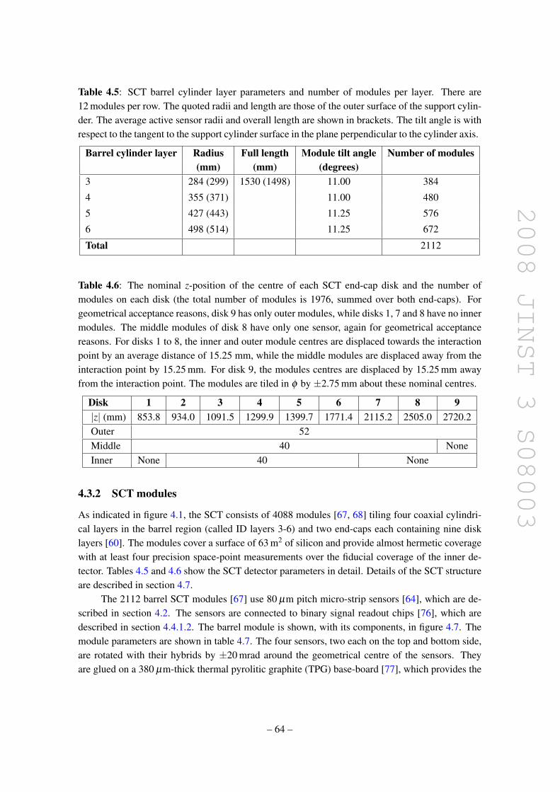
2008 JINST 3 S08003

Table 4.5: SCT barrel cylinder layer parameters and number of modules per layer. There are12 modules per row. The quoted radii and length are those of the outer surface of the support cylin-der. The average active sensor radii and overall length are shown in brackets. The tilt angle is withrespect to the tangent to the support cylinder surface in the plane perpendicular to the cylinder axis.

Barrel cylinder layer Radius Full length Module tilt angle Number of modules(mm) (mm) (degrees)

3 284 (299) 1530 (1498) 11.00 384

4 355 (371) 11.00 480

5 427 (443) 11.25 576

6 498 (514) 11.25 672

Total 2112

Table 4.6: The nominal z-position of the centre of each SCT end-cap disk and the number ofmodules on each disk (the total number of modules is 1976, summed over both end-caps). Forgeometrical acceptance reasons, disk 9 has only outer modules, while disks 1, 7 and 8 have no innermodules. The middle modules of disk 8 have only one sensor, again for geometrical acceptancereasons. For disks 1 to 8, the inner and outer module centres are displaced towards the interactionpoint by an average distance of 15.25 mm, while the middle modules are displaced away from theinteraction point by 15.25 mm. For disk 9, the modules centres are displaced by 15.25 mm awayfrom the interaction point. The modules are tiled in φ by ±2.75 mm about these nominal centres.

Disk 1 2 3 4 5 6 7 8 9|z| (mm) 853.8 934.0 1091.5 1299.9 1399.7 1771.4 2115.2 2505.0 2720.2Outer 52Middle 40 NoneInner None 40 None

4.3.2 SCT modules

As indicated in figure 4.1, the SCT consists of 4088 modules [67, 68] tiling four coaxial cylindri-cal layers in the barrel region (called ID layers 3-6) and two end-caps each containing nine disklayers [60]. The modules cover a surface of 63 m2 of silicon and provide almost hermetic coveragewith at least four precision space-point measurements over the fiducial coverage of the inner de-tector. Tables 4.5 and 4.6 show the SCT detector parameters in detail. Details of the SCT structureare described in section 4.7.

The 2112 barrel SCT modules [67] use 80 µm pitch micro-strip sensors [64], which are de-scribed in section 4.2. The sensors are connected to binary signal readout chips [76], which aredescribed in section 4.4.1.2. The barrel module is shown, with its components, in figure 4.7. Themodule parameters are shown in table 4.7. The four sensors, two each on the top and bottom side,are rotated with their hybrids by ±20 mrad around the geometrical centre of the sensors. Theyare glued on a 380 µm-thick thermal pyrolitic graphite (TPG) base-board [77], which provides the

– 64 –

2008 JINST 3 S08003

Figure 4.7: Photograph (left) and drawing (right) of a barrel module, showing its components. Thethermal pyrolytic graphite (TPG) base-board provides a high thermal conductivity path betweenthe coolant and the sensors.

thermal and mechanical structure. This extends sideways to include beryllia facings. A polyimidehybrid [78] with a carbon-fibre substrate bridges the sensors on each side. The two 770-strip (768active) sensors on each side form a 128 mm long unit (126 mm active with a 2 mm dead space).High voltage is applied to the sensors via the conducting base-board.

Precision alignment criteria were applied during assembly: the assembly tolerance as well asthe achieved build accuracy are shown in table 4.7. The important in-plane tolerance for positioningsensors within the back-to-back stereo pair was < 8 µm and the achieved variance was 2 µm. Inthe module plane, no additional distortions were measured after thermal cycling. Out-of-plane, theindividual components and the assembly jigging and gluing determine the module thickness andthe intrinsic bow of the sensors determines the out-of-plane shape. A common distortion profile hasbeen established for the sensors at the level of a few µm and a module thickness variation of 33 µmwas maintained during fabrication. Following thermal cycling, the out-of plane distortions changedby a few µm (RMS). When cooled from room to operating temperature, profile deviations did notexceed 20 µm, even at the sensor corners not supported by the base-board.

Figure 4.8 shows the construction of an end-cap module [68]. There are three module types,as shown in table 4.7. Each of the 1976 modules has two sets of sensors glued back-to-back arounda central TPG spine with a relative rotation of±20 mrad to give the required space-point resolutionin R-φ and R. The module thickness is defined by the individual components and variations arecompensated by the glue thickness (nominally 90 µm). The TPG spine conducts heat from thesensors to cooling and mounting points at the module ends and serves as the bias contact to thesensors. Glass fan-ins attach one end of the spine to a carbon base-plate with the polyimide flex-hybrid glued to it. The modules are arranged in tiled outer, middle and inner rings.

The precision alignment criteria applied to the end-cap modules were similar to those ofbarrel modules. The RMS spread of the module survey measurements after construction was 1.6µm in the back-to-back position of the stereo pair, measured transverse to the strips, and 2.8 µmin the position of the mounting hole and slot measured transverse to the strips. In the moduleplane, no additional distortions were measured after thermal cycling. Out of the plane, the end-

– 65 –

2008 JINST 3 S08003

Table 4.7: SCT barrel and end-cap module specifications and the RMS build accuracy for acceptedmodules. The barrel out-of-plane bowing specifications and the measured results are with respectto an average module shape. The quoted hybrid and sensor power consumption is more extensivelydescribed in section 4.5.

Parameter DescriptionStrips 2 × 768 active strips, ± 20 mrad stereo rotationNominal resolution 17 µm in-plane lateral (R-φ )

580 µm in-plane longitudinal (z or R)Module dimensions:-barrel Active length 126.09 mm + 2.09 mm dead space between sensors-outer end-cap Active length 119.14 mm + 2.09 mm dead space, radius 438.77−560.00 mm-middle end-cap Active length 115.61 mm + 2.09 mm dead space, radius 337.60−455.30 mm-short-middle end-cap Active length 52.48 mm, radius 402.82−455.30 mm-inner end-cap Active length 59.1 mm, radius 275.00−334.10 mmSpecified build Barrel back-to-back in plane: < 8 µm (lateral) < 20 µm (longitudinal)tolerance End-cap back-to-back in plane: < 5 µm (lateral) < 10 µm (longitudinal)

Barrel out-of-plane (module thickness and sensor bowing): < 70 µmBarrel envelope: < 200 µmEnd-cap envelope: < 115 µmBarrel module fixation points with respect to module centre: < 40 µmEnd-cap module fixation points with respect to module centre: < 20 µm

Build accuracy Barrel back-to-back in plane: ±2.1 µm (lateral) ±2.7 µm (longitudinal)of accepted End-cap back-to-back in plane: ±1.6µm (lateral) ±1.3 µm (longitudinal)modules (RMS) Barrel module thickness: ±33 µm

Barrel out-of-plane (sensor bowing): ±9 µmEnd-cap module thickness: ±15 µmEnd-cap out-of-plane (sensor bowing): ±20 µmBarrel module fixation points with respect to module centre ±10 µmEnd-cap module fixation points with respect to module centre ±6 µm

Hybrid power 5.5−7.5 WconsumptionSensor power Up to 460 V bias, < 1 W at –7Cconsumption

cap modules are less rigid, and are affected by variations of the spine thickness and bowing of thesensors. A common distortion profile has been established for the sensors at the level of a few µmand a module thickness variation of 15 µm was maintained during fabrication. Following thermalcycling, the out-of plane distortions changed by only a few µm (RMS). As for the pixels, thevariations within the module are small compared to the subsequent module-placement accuracies.

The spatial resolution of individual SCT modules has been measured in a test beam, forboth non-irradiated and fully irradiated modules [66]. At normal incidence, a combined spatialresolution of ∼16 µm is measured in R-φ ; the resolution is consistent with the binary readout ofthe two sensors with 80 µm strips, including a small fraction of multiple hits. The resolution isnot significantly degraded after irradiation. The barrel staves are mounted at a tilt angle of ∼ 11,

– 66 –

2008 JINST 3 S08003

Figure 4.8: The upper photograph shows the three SCT end-cap module types (outer, middle andinner from left to right). The lower schematic shows an exploded view of the different componentsfor a middle module, including the high thermal conductivity spine, the polyimide hybrid and theABCD readout ASIC’s.

defined by geometrical constraints and opposite in sign to that of the pixel barrel staves because ofthe different nature of the sensors used in each detector. The measured Lorentz angle, however, fora magnetic field of 2T, varies between 4.2 (before) and 2.7 (after) irradiation.

The barrel and end-cap sensors are specified to operate at −7C, with a maximum variationwithin and between modules of 5C, to reduce the bulk leakage current after radiation damage. Thehybrid power will be 5.5− 7.5 W per module, and the sensor load will reach ∼ 1 W per moduleafter ten years of operation. In addition, convective loads of ∼ 0.8 W per module plus ∼ 0.8 Wper module at the top of the barrel cylinders and outer disks are expected. The heat is extracted byevaporating C3F8 at ∼ −25C, circulating in cooling pipes attached to each module.

For the barrel, the sensor and hybrid heat leaves via the base-board and the hybrid substrateto the large beryllia facing on the base-board, which is interfaced to an aluminium block witha ∼100 µm layer of thermal grease and a copper-polyimide capacitive shunt shield. At full loadfor irradiated modules, the hybrid and sensor temperatures are expected to be approximately 14Cand 12C above the cooling-pipe temperature, respectively. The block is itself soldered to a 3.6 mmdiameter Cu/Ni cooling pipe. Each cooling loop serves 48 barrel modules.

For the end-cap, the sensor heat leaves via the spine, while the hybrid heat is transferred viathe carbon-fibre hybrid substrate to a carbon-carbon cooling block, which is split to minimise heat

– 67 –

2008 JINST 3 S08003

Table 4.8: Parameters of the TRT barrel modules and end-cap wheels (for one TRT end-cap).The quantities shown in bold are global parameters, including services and electronics. All otherquantities are for individual modules and the active region. Type-1 barrel modules include twostraw types, as described in the text.

|z|min |z|max Rmin Rmax Number Number Straws per(mm) (mm) (mm) (mm) of modules of layers module

Barrel (both sides) 0 780 554 1082 96 73 52544Type-1 module (inner) 400 712.1 563 624 32 9 329

Type-1 module (outer) 7.5 712.1 625 694 10

Type-2 module 7.5 712.1 697 860 32 24 520

Type-3 module 7.5 712.1 863 1066 32 30 793

End-cap (one side) 827 2744 615 1106 20 160 122880Type-A wheels 848 1705 644 1004 12 8 6144

Type-B wheels 1740 2710 644 1004 8 8 6144

transfer between the sensor and the hybrid. At full load, the ASIC and sensor temperatures areexpected to be respectively ∼ 30C and ∼ 10−15C above the coolant temperature. A layer ofthermal grease is applied between the modules and the cooling block. The blocks are soldered to aCu/Ni cooling pipe that serves up to 33 modules.

All modules were tested electrically at room temperature and at the expected operating tem-perature of−7C. Thermal cycling was performed on each module prior to completion of electricaltesting. After module assembly and testing, 99.8% of the strips operate satisfactorily.

4.3.3 TRT modules

The TRT contains up to 73 layers of straws interleaved with fibres (barrel) and 160 straw planesinterleaved with foils (end-cap), which provide transition radiation for electron identification. Allcharged tracks with pT > 0.5 GeV and |η | < 2.0 will traverse at least 36 straws, except in thebarrel-end-cap transition region (0.8 < |η | < 1.0), where this number decreases to a minimum of22 crossed straws. Typically, seven to ten high-threshold hits from transition radiation are expectedfor electrons with energies above 2 GeV.

The barrel TRT is divided into three rings of 32 modules each, supported at each end by aspace frame, which is the main component of the barrel support structure (see section 4.7). Eachmodule consists of a carbon-fibre laminate shell and an internal array of straws embedded in amatrix of 19 µm-diameter polypropylene fibres serving as the transition radiation material. Thestraws, described in section 4.2, form a uniform axial array with a mean spacing of ∼7 mm. Themodule shells are non-projective to reduce the dead region for high pT tracks. The main barrelparameters are shown in table 4.8. Figure 4.9 shows a quadrant of the TRT barrel during theintegration of the modules at CERN. A φ -slice showing one outer, one middle and one inner moduleis highlighted.

– 68 –

2008 JINST 3 S08003

The dimensional specifications are set by the intrinsic straw R-φ resolution of 130 µm, im-plying that each wire position is constrained to within ±50 µm. The module shell, made of400 µm thick carbon fibre with high thermal conductivity and flat to within 250 µm, is measuredto satisfy maximum distortions of < 40 µm under full load.

Figure 4.9: Photograph of one quarter of thebarrel TRT during integration. The shapes ofone outer, one middle and one inner TRT mod-ule are highlighted. The barrel support structurespace-frame can be seen with its triangular sub-structure.

The module shells also serve as a gasmanifold for CO2 which circulates outside thestraws to prevent high-voltage discharges andthe accumulation of xenon due to possible gasleaks which would absorb the transition radia-tion photons. The heat dissipated by the bar-rel straws is transferred to the module shellby conduction through the CO2 gas envelope.Each module shell is cooled by two coolingtubes located in the acute corners. These tubesalso serve as return pipes for the C6F14 coolingcircuits of the front-end electronics.

The module end with its components isshown in figure 4.11. The central element is theHV plate which has stringent requirements onflatness and cleanliness to prevent dischargesand on the straw feed-through accuracy to en-sure mechanical precision of the straw location.The HV plates were individually surveyed af-ter machining. The tension plate of figure 4.11mounted on the HV plate is a printed-circuitboard holding the wire ends (and ensuring the wire tension) and providing electrical connections.It also closes the active gas volume and serves as a Faraday cage for the active module elements.

Mechanical and electrical tests on the modules and individual straws were made at succes-sive assembly stages and following delivery of the modules to CERN. The module lengths wererequired to be in the range 1461.5–1462.9 mm and the twisting of individual modules was re-quired to be < 1 mm. Stringent criteria were applied to the gas tightness, wire tension, strawstraightness, and high voltage stability. The modules installed in the barrel had 98.5% operationalchannels.

The TRT end-caps each consist of two sets of independent wheels (see figure 4.10 and ta-ble 4.8). The set closer to the interaction point contains 12 wheels, each with eight successivelayers spaced 8 mm apart. The outer set of wheels contains eight wheels, also with eight strawlayers but spaced 15 mm apart. Each layer contains 768 radially oriented straws of 37cm lengthwith uniform azimuthal spacing. The space between successive straw layers is filled with layersof 15 µm thick polypropylene radiator foils separated by a polypropylene net.

Each eight-plane wheel consists of two basic four-plane assembly units. To assemble a four-plane wheel, straws were inserted and glued into precisely drilled holes in grounded inner and outercarbon fibre rings. The rings and the straws constitute the main mechanical structure of the wheels.The successive straw layers, interleaved by the radiators, are rotated from one layer to the next

– 69 –

2008 JINST 3 S08003

by 3/8 of the azimuthal straw spacing in a given layer. For high-pT prompt tracks, this ensuresoptimal uniformity in the number of crossed straws, which varies radially from ∼ six to ∼ fourstraws across an eight-plane wheel.

Figure 4.10: Photograph of a four-plane TRTend-cap wheel during assembly. The inner andouter C-fibre rings can be seen, as well as the firstlayer of straws and the first stack of polypropy-lene radiator foils beneath it. Also visible are theplastic end-plugs which are used to position andfix the straws to the C-fibre outer ring. The high-voltage petals used to connect the straws to thehigh-voltage lines (see text) are laid back at thisstage of the assembly and will only be folded ver-tically to push the petals into the straws at the nextstage.

Flex-rigid printed-circuit boards providehigh-voltage and signal connections to the end-cap wheels through two separate layers, asshown in figure 4.12. Each of the flexible lay-ers has conducting paths on one side whichconnect to the rigid part of the board. To pro-vide a reliable electrical connection, flexible"petals" in the high-voltage layer are forcedinto contact with the inner straw wall throughthe insertion of a plastic plug [71]. A press-fitbetween similar but smaller petals in the signallayer and a metallic crimping pin positions andfixes the anode wires. There are 32 such boardsper four-plane wheel, each serving a φ -sectorof 96 straws.

Each sector is further segmented intothree groups of 32 readout channels and12 high-voltage groups of eight straws sharinga common fuse and blocking capacitor. Thecarbon-fibre ring holding the straws and flex-rigid boards, together with a third carbon fibrering and a simpler glass fibre board provide arigid structure around the outer wheel perime-ter that also serves as a gas manifold (see fig-ure 4.12). The inner gas manifold is made fromreinforced polyimide material.

The heat dissipated by the end-cap strawsis evacuated through the CO2 gas envelopewhich is forced to flow along the straws fromthe inner to the outer radius. Each group ofwheels has its own CO2 cooling circuit, pass-ing the gas sequentially through all the wheelsof the group. Heat exchangers cooled with C6F14 extract heat from the gas between adjacentwheels. The high flow rates required, 50 m3 per hour for type-A and 25 m3 per hour for type-Bwheels, necessitates a closed-loop system capable of maintaining a small gas pressure between 0and 5 mbar with a stability of ±0.5 mbar inside the detector.

As for the barrel modules, all end-cap wheels passed quality control procedures during con-struction and after delivery to CERN, resulting in more than 99% of fully operational channels.

– 70 –

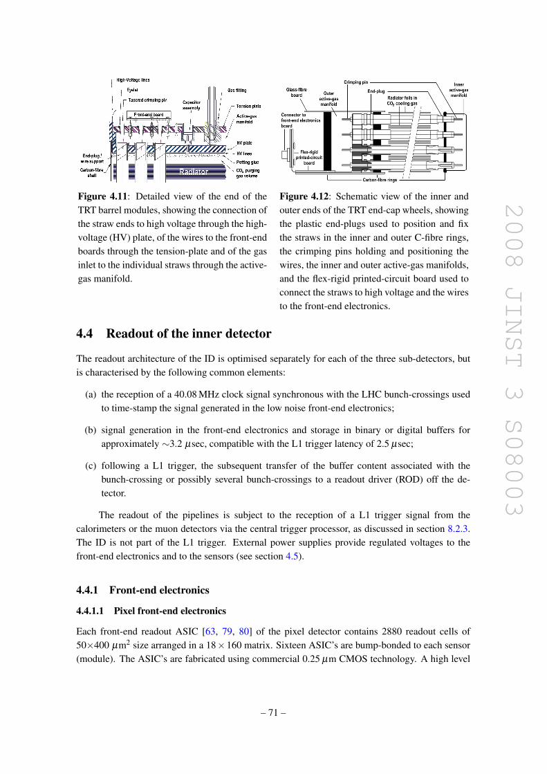
2008 JINST 3 S08003

Figure 4.11: Detailed view of the end of theTRT barrel modules, showing the connection ofthe straw ends to high voltage through the high-voltage (HV) plate, of the wires to the front-endboards through the tension-plate and of the gasinlet to the individual straws through the active-gas manifold.

Figure 4.12: Schematic view of the inner andouter ends of the TRT end-cap wheels, showingthe plastic end-plugs used to position and fixthe straws in the inner and outer C-fibre rings,the crimping pins holding and positioning thewires, the inner and outer active-gas manifolds,and the flex-rigid printed-circuit board used toconnect the straws to high voltage and the wiresto the front-end electronics.

4.4 Readout of the inner detector

The readout architecture of the ID is optimised separately for each of the three sub-detectors, butis characterised by the following common elements:

(a) the reception of a 40.08 MHz clock signal synchronous with the LHC bunch-crossings usedto time-stamp the signal generated in the low noise front-end electronics;

(b) signal generation in the front-end electronics and storage in binary or digital buffers forapproximately ∼3.2 µsec, compatible with the L1 trigger latency of 2.5 µsec;

(c) following a L1 trigger, the subsequent transfer of the buffer content associated with thebunch-crossing or possibly several bunch-crossings to a readout driver (ROD) off the de-tector.

The readout of the pipelines is subject to the reception of a L1 trigger signal from thecalorimeters or the muon detectors via the central trigger processor, as discussed in section 8.2.3.The ID is not part of the L1 trigger. External power supplies provide regulated voltages to thefront-end electronics and to the sensors (see section 4.5).

4.4.1 Front-end electronics

4.4.1.1 Pixel front-end electronics

Each front-end readout ASIC [63, 79, 80] of the pixel detector contains 2880 readout cells of50×400 µm2 size arranged in a 18×160 matrix. Sixteen ASIC’s are bump-bonded to each sensor(module). The ASIC’s are fabricated using commercial 0.25 µm CMOS technology. A high level

– 71 –

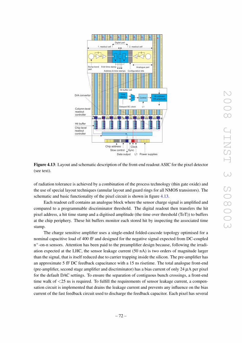
2008 JINST 3 S08003

Chip-levelreadoutcontroller

Hit buffer

Column-levelreadoutcontroller

Data output

Clock

L1 Power supplies

8-bit time stamp

Address & time stamps

1. readout cell 2. readout cell

Analogue part

Configuration bits

Digital part

Time

Delayed BC clock L1

?Hit address

Hit amplitudeControl

Hit buffer cell

D/A convertor

Bump-bondpad

Slow control

Chip address

Sync

stamp

Figure 4.13: Layout and schematic description of the front-end readout ASIC for the pixel detector(see text).

of radiation tolerance is achieved by a combination of the process technology (thin gate oxide) andthe use of special layout techniques (annular layout and guard rings for all NMOS transistors). Theschematic and basic functionality of the pixel circuit is shown in figure 4.13.

Each readout cell contains an analogue block where the sensor charge signal is amplified andcompared to a programmable discriminator threshold. The digital readout then transfers the hitpixel address, a hit time stamp and a digitised amplitude (the time over threshold (ToT)) to buffersat the chip periphery. These hit buffers monitor each stored hit by inspecting the associated timestamp.

The charge sensitive amplifier uses a single-ended folded-cascode topology optimised for anominal capacitive load of 400 fF and designed for the negative signal expected from DC-coupledn+-on-n sensors. Attention has been paid to the preamplifier design because, following the irradi-ation expected at the LHC, the sensor leakage current (50 nA) is two orders of magnitude largerthan the signal, that is itself reduced due to carrier trapping inside the silicon. The pre-amplifier hasan approximate 5 fF DC feedback capacitance with a 15 ns risetime. The total analogue front-end(pre-amplifier, second stage amplifier and discriminator) has a bias current of only 24 µA per pixelfor the default DAC settings. To ensure the separation of contiguous bunch crossings, a front-endtime walk of <25 ns is required. To fulfill the requirements of sensor leakage current, a compen-sation circuit is implemented that drains the leakage current and prevents any influence on the biascurrent of the fast feedback circuit used to discharge the feedback capacitor. Each pixel has several

– 72 –

2008 JINST 3 S08003

parameters that are tuned and stored in a 14-bit control register, for example the feedback trimmingand threshold levels. The digital circuitry in the readout cells generates the required hit informationto measure the charge and associate the hit to the bunch crossing.

The readout is made using the column-based readout controller. The first task of the controlleris the generation of the readout sequence to transfer the hit information from the pixel to the hitbuffer at the end of the column. The second task is the digital processing of hit data in the front-endchip buffers. Hits are continuously compared to a delayed beam-crossing counter (see figure 4.13).When a match is found with the correct latency, the hit is flagged for readout if a L1 trigger signalis present, or deleted if there is no matching trigger. Flagged hits are transmitted to a serialiserand sent out of the chip. Hits older than the trigger latency are cleared from the front-end chipbuffers.

The module-control chip [63, 81] is a digital chip running with the same 40 MHz clock. Ithas three main system tasks: the loading of parameter and configuration data in the front-end chipsand in the module-control chip itself, the distribution of timing signals such as bunch-crossing, L1trigger and resets (TTC functions), and the front-end chip readout and event building. The designof the module-control chip reflects the required pixel performance during LHC operation: theassociation of signals to a bunch-crossing, the expected bandwidths at the highest luminosity, themaximum L1 trigger rate of 100 kHz (initially 75 kHz) and the number of front-end chips, whichare controlled in a module. Because of the high radiation environment, particularly in layer−0modules, special attention has been given to ensure a single-event upset (SEU) tolerant design.

Extensive electrical tests have been made on ASIC chips, single front-end chip assembliesand full modules, before and after irradiation. Some production modules were irradiated to theend-of-life dose expected at LHC. The noise and hit efficiency are shown in figure 4.14 for a pixelmodule before irradiation. Similar results are also shown for a module irradiated to a fluence Fneq

of 1015cm−2(and to 500 kGy ionising dose) in a 24 GeV proton beam, at an operating temperatureof -4C and after threshold retuning. Both quantities are only slightly deteriorated by the irradiationand remain within the operating specifications. Furthermore, the difference in threshold dispersionafter retuning is negligible.

4.4.1.2 SCT front-end electronics

The readout hybrid of each SCT module (see section 4.3) houses 12 identical 128-channelASIC’s [76] to read a total of 1536 sensor strips per module. The ASIC is fabricated in radia-tion tolerant bi-CMOS DMILL technology. The successive blocks of the ASIC are shown in thecircuit schematic of figure 4.15. A pre-amplifier, shaper and tunable discriminator exists for eachchannel. A 132-length binary pipeline stores the hit information for each channel associated to thebeam crossing for a period of ∼3.2 µsec. Following a L1 trigger, the chip compresses the datapertinent to that beam crossing and serialises it for output. An 8-deep de-randomising buffer afterthe pipeline ensures that the dead-time is negligible for the expected data rates.

Two critical module performance specifications are the detection efficiency (> 99%) andnoise occupancy (< 5×10−4), for signals from the 12 cm long silicon strips with a capacitive loadof ∼ 20 pF. These have led to the choice of a front-end discriminator threshold of 1 fC. Extensivestudies have been made using ASIC chips, single front-end chip assemblies and full modules,before and after irradiation. A sample of production modules was irradiated in a 24 GeV proton

– 73 –

2008 JINST 3 S08003

Time (ns)

Eff

icie

nc

y

Noise (e)140 160 180 200 220 240

1000

2000

3000

4000

5000

Mean = 185

Noise (e)140 160 180 200 220 240 260 280 0 10 20 30 40 50 60 70 80

0 10 20 30 40 50 60 70 80

500

1000

1500

2000

2500

3000

3500

4000

4500

Mean = 209

Time (ns)

Eff

icie

nc

y

Eff. = 99.90 ± 0.15 %

Eff. = 98.23 ± 0.15 %

Even

tsE

ven

ts

0.2

0

0.4

0.6

0.8

1.0

0.2

0

0.4

0.6

0.8

1.0

Noise (electrons) Time (ns)

Noise (electrons) Time (ns)

Eve

nts

Eve

nts

Eff

icie

ncy

Eff

icie

ncy

Figure 4.14: Noise distribution for normal pixels of a non-irradiated module (upper left) and of amodule irradiated with 24 GeV protons to a fluence Fneq of 1015cm−2 (lower left), measured afterretuning at an operating temperature of−4C. The measured efficiency as a function of the incidentbeam particle arrival time is also shown for the non-irradiated (upper right) and irradiated modules(lower right). The arrows indicate the efficiency at the timing plateau.

beam to a dose of ∼3×1014 protons per cm2, equivalent to the damage expected for a fluence Fneq

of 2×1014 cm−2. The efficiency and noise occupancy measured in a test-beam are shown as afunction of the discriminator threshold in figure 4.16. At the nominal operating threshold of 1 fC,the efficiency and noise-occupancy specifications are easily met before irradiation and almost metafter irradiation.

The chips are daisy-chained so that all the data of one module are read out over two seriallinks. Several design features provide fault tolerance. For example, any faulty chip (except forthe master on barrel modules) can be bypassed in the serial data path and if one link should fail,it is possible to send the data using the remaining active link. Likewise, if the primary clock andcommand lines to the ASIC’s on a module fail, it is possible to instead use the clock and commandsignals from an adjacent module.

– 74 –

2008 JINST 3 S08003

Φ3

Φ1

Φ2

Datain

logiccontrolBuffer

Write pointerL1

Data out24 x 128

Block of RAM

Read pointer

L1

Data available

Overflow

Error

Read

Read

Mask register

Derandomiser buffer

Co

mm

and

amplifier and comparator128 channel transimpedance

deco

der

Dyn

amic

FIF

O

Comparator

Front−end

Threshold

Data

Mask register

Data in

"1"

Edge detecting circuit

Mask

Load

Data out

Masking logic

Q

Q’

D

BCO

LevelEdge/

Test mode

Test pulse

D Q

Q’

D Q

Q’

CLK

Q

CLK

DQ

CLK

DQ

CLK

DQ

CLK

DQ

CLK

DQ

CLK

DQ

CLK

DQ

CLK

DQ

D

DA

C’s

& C

alibratio

n

Data compression& serialiser

Read

ou

t con

troller

D1

D0

Figure 4.15: Schematic of the readout ASIC for the SCT detector, showing the successive signalprocessing steps.

Corrected threshold (fC)0.7 0.8 0.9 1 1.1 1.2 1.3 1.4

Eff

icie

ncy

0.9

0.91

0.92

0.93

0.94

0.95

0.96

0.97

0.98

0.99

1

No

ise

occ

up

ancy

10-6

10-5

10-4

10-3

10-2

10-1

1

Corrected threshold (fC)0.7 0.8 0.9 1 1.1 1.2 1.3 1.4

Eff

icie

ncy

0.9

0.91

0.92

0.93

0.94

0.95

0.96

0.97

0.98

0.99

1

No

ise

occ

up

ancy

10-6

10-5

10-4

10-3

10-2

10-1

1

Figure 4.16: The efficiency (circles) and noise occupancy (triangles) for SCT barrel modules mea-sured in a test-beam before irradiation (left) and after exposure to a dose of ∼ 3×1014 p/cm2 in a24 GeV proton test-beam (right). The nominal operating threshold is 1 fC. The dashed horizontallines represent the nominal module performance specifications in terms of efficiency and noise.The vertical lines represent the range of thresholds over which these specifications are met afterirradiation.

– 75 –

2008 JINST 3 S08003

Figure 4.17: Schematic of the front-end readout of the TRT detector, showing the input signalshape and the signal shape after the amplification and shaping, the baseline restoration (BLR)and the dual-threshold discrimination which provides the ternary output corresponding to the lowthreshold set or both low and high thresholds set.

4.4.1.3 TRT front-end electronics

The analogue signal processing and threshold discrimination to detect signals from both minimum-ionising particles and transition radiation, as well as the subsequent time digitisation and data-pipelining are implemented in two on-detector ASIC’s. The signal is shown in figure 4.17 at eachstage of the TRT signal readout chain which comprises:

(a) an eight-channel analogue ASIC [82], called the ASDBLR, fabricated in bi-CMOS radiationtolerant DMILL technology. It performs the amplification, shaping and baseline restora-tion. It includes two discriminators, one operating at low threshold (typically 250 eV) forminimum-ionising signal detection and one operating at high threshold (typically 6 keV) fortransition radiation detection;

(b) a subsequent 16-channel ASIC fabricated in commercial radiation-tolerant 0.25µm CMOStechnology [83]. This ASIC performs the drift-time measurement (∼ 3 ns binning). It in-cludes a digital pipeline for holding the data during the L1 trigger latency, a derandomisingbuffer and a 40 Mbits/s serial interface. It also includes the necessary interface to the timing,trigger and control as well as DAC’s to set the discriminator thresholds of the analogue ASICand test-pulse circuitry for mimicking analogue inputs to the analogue ASIC.

These ASIC’s are housed on front-end boards attached to the detector. There are 12 differentboards for the barrel and three different boards for the end-cap. The electronics are cooled by aliquid mono-phase fluorinert (C6F14) cooling system.

– 76 –

2008 JINST 3 S08003

P P 1

T y p e I I c a b l e s1 3 6 L V c a b l e s3 0 4 D C S c a b l e s

1 0 - 1 3 mC r y o s t a t i n n e r b o r e

T y p e I V c a b l e s4 0 2 D C S & S e r v i c e s

c a b l e s5 0 - 5 5 m

T y p e I I I c a b l e s1 3 6 L V c a b l e s

4 0 - 7 5 m3 0 4 D C S & I n t e r l o c k

c a b l e s2 5 - 4 0 m

P P 0 T y p e I c a b l e s2 8 0 H V a n d L V c a b l e s

3 0 4 D C S c a b l e s2 9 4 8 - w a y r i b b o n f i b r e s

3 m

P a t c h P a n e l I Ii n s i d e t h e m u o n s p e c t r o m e t e r

S l o w - c o n t r o l e l e c t r o n i c sV o l t a g e r e g u l a t o r s

T y p e I I I c a b l e s1 4 4 H V c a b l e s

4 2 6 4 - f i b r e o p t i c a l c a b l e s6 0 - 9 0 m

P P 2

U S 1 5U S A 1 5

P P 3

Figure 4.18: The routing of data links and power supply cables from each side of the pixel detectorto respectively the off-detector electronics and power supplies in the service caverns, together withthe number, type and utilisation of the cables and optical links.

At the TRT operating low threshold used for tracking (equivalent to ∼ 15% of the averagesignal expected from minimum-ionising particles), the mean straw noise occupancy is ∼ 2%, but asmall fraction of 1% of channels have a noise occupancy exceeding 10%, which however remainssmall compared with the expected maximum straw occupancy of 40%. The full front-end electron-ics chain was exposed to a neutron dose of ∼4×1014/cm2 and to a γ-ray dose of 80 kGy. Changesof up to 25% were observed in the ASDBLR gain, but with no change in the effective thresholdsand noise performance after a standard voltage compensation procedure.

4.4.2 Data transmission and power-supply services and routing

The transmission of data from the ID modules to the off-detector electronics in the service cavern,as well as the digital transmission of the clock and control commands to the modules differs for the3 sub-detectors. Figures 4.18, 4.19 and 4.20 summarise the layout and technology of the readoutand control services for each of the pixel, SCT and TRT sub-detectors. The locations of key patch-panel connection boards are shown: PP0 close to the ends of the pixel detector, PP1 at the edgesof the ID volume, PP2 in specifically designed parts of the muon spectrometer system and PP3outside the ATLAS active detector volume. The numbers and lengths of lines for each module(pixel, SCT) or front-end board (TRT) are tabulated for both the barrel and end-caps. Similarly, thecables used for the readout electronic bias as well as the silicon sensor and TRT straw high-voltagelines are also shown.

– 77 –

2008 JINST 3 S08003

PPB1

PPF1

Type II cables2044 Power cables

20 m72 96- or 72-fibre optical cables

69 - 91 m128 14-pair DCS cables

33 - 51 m

Cryostat inner bore

Balconiesin UX15

US15

USA15

Type IV cables2044 Power cables

40 m4 CANbus & 48 Interlock cables

36 - 71 m

Type III cables2044 Power cables

40 m

PPF0

Type I cables988 Low-mass power tapes266 12-way ribbon fibres

748 DCS wires1.4 - 3.2 m

PP3

Limiters

&

Filters

Power cablesplices

Type I cables1056 Low-mass power tapes

264 12-way ribbon fibres826 DCS wires

0.9 - 1.9 m

DCS

PP2

Figure 4.19: The routing of data links and power supply cables from each side of the SCT torespectively the off-detector electronics and power supplies in the service caverns, together withthe number, type and utilisation of the cables and optical links.

P P B 1

P P F 1

T y p e I I c a b l e s1 2 9 2 m i n i - c o a x i a l H V l i n e s

3 5 2 0 L V c a b l e s1 5 9 3 6 m i n i a t u r e t w i s t e d p a i r s f o r d a t a r e a d o u t , T T C a n d D C S

1 2 - 1 5 m

C r y o s t a t i n n e r b o r e

P P 2

M A R A T O ND C - D C

B a l c o n i e s i n U X 1 5

U S A 1 5

P a t c h P a n e l I Ii n s i d e t h e m u o n s p e c t r o m e t e r

E l e c t r i c a l t o o p t i c a l c o n v e r t e r s L V D S r e p e a t e r s

S l o w - c o n t r o l e l e c t r o n i c sV o l t a g e r e g u l a t o r s

T y p e I I I c a b l e s3 4 H V m u l t i - c o n d u c t o r c a b l e s

3 2 C A N B u s c a b l e s2 8 8 M u t i - p a i r c a b l e s

9 6 4 - f i b r e o p t i c a l c a b l e s6 0 - 1 0 0 m

T y p e I V c a b l e s1 2 M u l t i - p a i r c a b l e s1 2 3 8 0 V c a b l e s

3 5 - 6 0 m

T y p e I I I c a b l e s5 4 4 L V c a b l e s2 5 - 4 0 m

Figure 4.20: The routing of data links and power supply cables from each side of the TRT torespectively the off-detector electronics and power supplies in the service caverns, together withthe number, type and utilisation of the cables and optical links.

– 78 –

2008 JINST 3 S08003

RX plug-in

TX plug-in

DORIC

Opto-board

Opto-board

Up

Down

LVDSPP0 PP1

rackROD

16 or 8

8

84

4

(8)

8

8

8

272

272

272

272

Back-of-Crate Card

VDC

6 or 71 or 2

2 or 4

272

2

PIN

array

VCSEL

array

Fibres Fibres

PIN

array

VCSEL

array

DRX

BPM-12

Module

MCC

Figure 4.21: Detailed schematic of the pixel optical link architecture. For each pixel module, one(layer-1, layer-2 and the disks) or two (layer-0) optical fibres transfer data to the ROD’s, and onefibre transfers the control and clock signals to the module (see text). The SCT optical links have asimilar design.

4.4.2.1 Pixel and SCT readout

The digital transmission of the clock and control commands to the pixel and SCT module and datafrom the module to off-detector electronics in the service cavern is made via optical links [76, 84–86]. A detailed block diagram illustrating the pixel link structure is shown in figure 4.21.

As summarised in table 4.9 each pixel module uses one or two up-link fibres according tothe required bandwidth; the bit rate is either 40 or 80 Mbits/s per fibre link. One down-link fibreper module is used to transmit trigger, timing, clock signals and configuration data. Opto-boardson the detector side convert the electrical signals from the module-control chip to optical signals.The down-link uses a bi-phase mark encoded format to transmit both the 40 MHz bunch-crossingclock and the data. The bi-phase mark light signal, detected by a PIN diode, is decoded by adigital opto-receiver integrated circuit (the DORIC chip). In the up-link the module-control chipoutput is converted to light by a driver chip coupled to a vertical-cavity surface-emitting laserdiode (VCSEL). This latter chip and the corresponding SCT chips have four channels each. Theyhave been made in the same 0.25 µm CMOS technology as the module-control chip and havebeen produced on the same silicon wafers. Opto-boards can service either six (half-staves or disk-sectors) or seven (half-staves) modules depending on which part of the detector they are connectedto. The opto-boards have been placed on service quarter-panels near the internal surface of thepixel support tube (see section 4.7), to reduce the radiation dose collected over ten years of LHCoperation.

In the case of SCT modules, the service harness that provides power to 4–6 modules alsoincludes two data fibres and one trigger/control fibre for each module, as well as VCSEL andPIN diode opto-packages for electrical to optical conversion together with their control ASIC’s.Each SCT barrel module is serviced by a polyimide-aluminium low-mass tape which providesredundancy and electrically isolates the modules. For the end-caps, polyimide-copper tapes areused for the control lines and copper-clad aluminium twisted pairs for the power lines, from themodule to the edge of the disk. The module is then connected via polyimide-copper tape to thePP1 patch-panel outside the SCT and from there by conventional cables to the power supplies.

– 79 –

2008 JINST 3 S08003

Table 4.9: Summary of the main characteristics of the optical links used for the pixel and SCTdata readout and trigger, timing and control (TTC) signals (NRZ stands for Non-Return to Zeroand BPM for Bi-Phase Mark).

Sub-detector Link Speed Format Links per module Number of links(Mbits/s)

Pixels Data 40/80 NRZ 1 (layer-1, 2 and disks) 1458

40/80 NRZ 2 (layer-0) 572

TTC 40 BPM 1 1744

SCT Data 40 NRZ 2 8176

TTC 40 BPM 1 4088

On the other side of the link, back-of-crate (BOC) cards interface the opto-signals with theelectrical signals in the readout driver (ROD). These cards are the same for the pixel and SCT de-tectors and they contain two kinds of electro/optical converter plug-ins: a RX plug-in with an arrayof PIN diodes and a data receiver, and a TX plug-in with an array of VCSELs driven by a bi-phase mark encoding ASIC. The SCT uses a radiation-hard step index multi-mode fibre for thefull length from the back-of-crate cards to the detector. The pixel detector uses a long length ofradiation-tolerant graded-index fibre, spliced to 7 m lengths of the radiation-hard fibre inside thedetector.

4.4.2.2 TRT readout

As described in section 4.3.3, the TRT readout is segmented in 32 φ -sectors in order to simplifythe data transmission for L2 triggers. The initial 40 Mbits/s LVDS data readout uses small customdesigned twisted pair lines from the ASIC to the boards at patch panel PP2, located after the firstmuon chambers. The data are then serialised in a Gbit serialiser [87] and an electrical-to-opticalconversion is made. The complete readout of the TRT requires 768 1.6 Gbits/s optical links. Timingand control signals are electrically transmitted to and from the TRT-TTC module.

4.4.2.3 Pixel, SCT and TRT readout drivers

As described in section 8.3.5, all readout driver modules (ROD’s) receive serialised data from thedetector upon reception of a L1 trigger, perform de-serialisation, error checking, data compression(in the case of the TRT), and local event-building and data-monitoring tasks. The ROD’s combinethe data received into a single event packet associated to the L1 trigger. The event packets aretransferred in a standard data format over a high-speed optical link, the ATLAS S-link, to thereadout system, which is common to all ATLAS sub-detectors.

Each pixel and SCT ROD crate is a 9U VME crate with up to 16 ROD’s per crate. Each RODis paired with a back-of-crate card, which is plugged into the crate back-plane and provides the op-tical to electrical interfaces [85, 88, 89]. The back-of-crate card can accept both 40 Mbits/s optical

– 80 –

2008 JINST 3 S08003

links from pixel and SCT modules and 80 Mbits/s from pixel modules. Each ROD card servicesup to 48 SCT modules (96 data links) or between 6 and 26 pixel modules, depending on theirgeometrical location. The lower number of pixel modules serviced per ROD is due to the largerquantity of data received from pixel modules at the smallest radius, due to their higher occupancy.The number of modules which can be processed by one ROD is limited by the output bandwidth ofthe S-link. The pixel and SCT ROD’s are identical units except for the data-treatment algorithms.The ROD crates receive clock, trigger and fast commands from the ATLAS TTC system through aTTC interface module (TIM), located in each crate which transmits these signals across the crate,using a custom back-plane, to the ROD’s and back-of-crate cards. Clock and command signals arethen transmitted to the detector modules using a simpler protocol over the optical fibres mentionedabove.

The TRT off-detector electronics also uses two custom-designed TRT-ROD and TRT-TTCmodules [90]. Each ROD receives serialised data from 1/16 of one barrel side or 1/32 of one end-cap side, using eight optical links operating at 1.6 Gbits/s. After the optical-to-electrical conver-sion, the ROD’s perform the standard tasks described above, including a data-compression schemewhich does not introduce any data losses. The TRT-TTC module provides an interface betweenthe standard ATLAS TTC system and the TRT front-end electronics. It also feeds the ROD withall necessary L1 trigger information (event ID, bunch crossing ID, trigger type). Each TRT-TTCmodule interfaces to the front-end using 40 links and to two ROD’s via a dedicated back-planeusing the VME 9U P3 connector.

4.5 Electronics and detector power supplies and services

Both the sensors and the front-end electronics of the inner detector require substantial power forinitial operation and the power load will increase during the high-luminosity operation. Table 4.10,together with figures 4.18 to 4.20, summarise the requirements for each of the pixel, SCT and TRTsub-detectors, in terms of bias voltage for the silicon sensors or high voltage for the straws (HV)and of low voltage (LV) for the front-end electronics, as well as the segmentation and routingused for the power distribution. The power distribution lines are connected at PP0 and PP1 on thecryostat wall, at PP2, which is external to the inner-detector volume and located after the first muonchambers, and at PP3 on the outside of the whole detector.

The pixel power supply system has four main components: the LV and HV power supplies,the regulator stations, and the supply and control for the opto-links. Two commercial LV suppliesprovide the analogue and digital parts of the front-end readout electronics. To protect the front-endelectronics against transients, remotely-programmable and radiation-tolerant regulator stations areinstalled at PP2. Separate HV supplies are able to power the sensors up to 700 V with a maximummodule current of 4 mA. The worst-case expected module operating condition is a 600 V depletionvoltage with a 2 mA leakage current. The LV and HV lines are connected to respectively thelow-voltage and high-voltage patch-panels which distribute the power and monitor the currents ofindividual lines. The supply and control of the optical link is a complex link in itself, consisting ofthree voltage sources and a control signal. It delivers the adequate levels for the operation of theon-detector part of the optical link.

– 81 –

2008 JINST 3 S08003

Table 4.10: Summary of the silicon sensor bias voltage, straw-tube high-voltage and front-endelectronics requirements and granularity. The different front-end electronic supply voltages aredescribed in the text. The power consumption expected during initial operation is also shown.Following irradiation, the power consumption increases significantly in the sensors, front-end elec-tronics and cables (see text). Additional power requirements to ensure thermal isolation in theID volume are described in the text.

Pixel SCT TRTVoltage (maximum) 700 V 500 V 2000 V

Bias or Voltage (nominal) 150–600 V 150–350 V 1600 Vhigh-voltage Current (maximum) 4 mA 5 mA 3 mAsupplies Segmentation One per module One per module One per ∼ 200 straws

1744 channels 4088 channels 1984 channels1.7–2.1 V analogue 3.5 V analogue ±3 V analogue

Voltages 2.1–2.5 V digital 4 V digital 2.5 V digital0.8, 2.5, 10 V opto-device 5, 10 V opto-device

Front-end Current 3.7 kA 6 kA 6.5 kAelectronics Segmentation Configurable One per module 1/32 of end-cap sidelow-voltage of bulk supply 6–7 modules 4088 channels 1/32 of barrel sidesupplies Segmentation One regulator See above One regulator per

of regulated per module 1/32 of wheel orsupplies per barrel moduleFront-end 6 kW 22 kW 22 kWelectronics powerCables plusregulators:

Power - in ID volume ∼ 4 kW ∼ 5 kW ∼ 3 kW- outside ID volume ∼ 14 kW ∼ 9 kW ∼ 20 kW- total cable loss ∼ 18 kW ∼ 14 kW ∼ 23 kW

(∼ 6V drop) (1.5–4.6 V drop) (3.8 V drop)Total power ∼ 24 kW ∼ 36 kW ∼ 44 kW(initial operation)

The SCT [91] maintains independent electrical services to each of the 4088 modules. Eachmodule receives multi-voltage LV channels providing power and control signals to the readoutchips, the optical electronics, timing and control electronics, as well as HV to the silicon sen-sors. The SCT LV power module provides the analogue and digital voltages for the SCT front-endASIC’s and optical-link components. Each LV power module also includes the hybrid temperaturereadout as well as the digital control lines. The HV bias provides a stable and controlled voltageof 0–500 V with a current limit of 5 mA. The LV and HV modules are based on DC-DC convert-ers with a single power line serving each module; twelve identical 4-channel LV and six identical8-channel HV boards are housed in each crate. Each board in the crate is connected through asystem-interlock card to the detector control system (see section 4.8.4). The four crates of eachrack are powered by four commercial power units (including one spare) connected in parallel toprovide a 48V DC supply. As an example for the barrel SCT, the power distribution lines are infour parts: low-mass polyimide tapes for the innermost region of the detector, which are connectedto PPB1 on the cryostat wall, thin cables along the cryostat wall, which are spliced to medium-sizecables outside the cryostat, and, after PP3, thick cables going to the power-supply crates. Becauseof the large voltage drop in the cables (up to 4.6 V), the supplied voltage exceeds the maximum

– 82 –

2008 JINST 3 S08003

allowed voltage of the ASIC’s. This could be problematic, for example in case of a drop in thepower consumption of the front-end system. To avoid such incidents, a voltage-limiter circuit hasbeen introduced at PP3. To dampen common-mode noise, inductors on all power and low-currentcontrol and monitoring lines are also housed at PP3.

The TRT front-end electronics require three low-voltage power supplies (+2.5 V digital and±3 V analogue). Commercial supplies deliver power to boards located at PP2. The PP2 boardshouse radiation-tolerant voltage regulators delivering power to each front-end board. The size ofthe cables feeding the PP2 power boards and the front-end boards is a compromise between theavailable space and the power dissipation in the cable trays allowed by the cooling system. TheTRT straw high voltage is nominally 1530 V. Sets of about 200 straws are powered by a singlecommercial HV source able to deliver up to 3 mA at 2 kV. A total of 1984 HV channels are neededfor the whole detector. Standard multi-wire HV cables are used up to the level of PP2, then customminiature HV cables are used to reach the detector.

The power dissipation during initial detector operation is also indicated in table 4.10. The ini-tial power dissipation from the front-end electronics and cables is ∼ 62 kW within the ID volume,and ∼104 kW in total. However, during high-luminosity operation of the TRT and after irradia-tion of the pixel and SCT sensors, several kilowatts of power are dissipated by the sensors (this issensitive to temperature for the silicon sensors). Together with additional losses in the cables andincreased front-end power consumption, the total power loss within the ID volume is expected toexceed 85 kW after several years of operation.

Additional power supplies are required for the pad heaters located on the thermal enclosuressurrounding the pixel and SCT detectors (see section 4.7.2) and for the heaters which are an integralcomponent of the evaporative cooling system for the pixel and SCT detectors (see section 4.8.3).The thermal enclosures require a total power of almost 30 kW, including the heaters surrounding thebeam-pipe (see section 4.8.1). The heaters for the cooling system require a total power of 126 kW,which is provided by four racks situated in the service caverns. These power supplies are controlledby programmable logic controllers, which regulate the entire system and manage, in particular,transients caused by changes in the power load as the detector electronics are switched on or off.

4.6 Grounding and shielding of the inner detector

The three components of the inner detector, the pixels, the SCT and the TRT are designed tobe electrically isolated both from earth and from each other, as is generally required for all AT-LAS components (see section 9.4.8). The detectors are therefore floating by design. This pro-vides the possibility of a controlled ground connection at a location identified as IDGND be-tween the tile calorimeter and the first layer of barrel muon chambers. A star connection ofall the safety grounding cables for ID components, as well as common items (support struc-ture, pipes for cooling and gas, heaters, and DCS sensors), ends in IDGND. The IDGND isconnected to the ATLAS equipotential network by means of a dedicated 95 mm2 conductor. Toprovide reasonable isolation of the sub-detectors and at the same time to complete the require-ments of the safety grounding, the connection to IDGND from any sub-detector is made fromits electromagnetic shield using a single-point connection. The power supplies are floating and

– 83 –

2008 JINST 3 S08003

Figure 4.22: Schematic top view of the inner-detector sub-systems with their vertical supportpoints. All supports are on the plane of the detector axis and symmetric with respect to this axis.

are referenced in most cases on the detector modules (analogue and digital grounds) and at thePP0 and PP1 patch-panels (connection of the detector-module grounds to the electromagneticshields).

Each pixel module is referenced at PP0, and all the PP0’s are grounded with both the elec-tromagnetic shield and the beam-pipe shield at PP1. The pixel detector itself is surrounded by aFaraday cage defined by an aluminium layer surrounding the beam-pipe, and an aluminium layersurrounding the outside of the pixel support tube. The PP1 end-plates close the Faraday cage atthe two ends and serve as the common grounding point for the pixel detector. There is a singlegrounding connection to IDGND on side-A of the detector. The SCT barrel and end-cap moduleassemblies are each enclosed by outer electromagnetic shield skins. The individual module supplytapes, outer supply cable shields and detector array shield skins are electrically bonded at PPB1(for the barrel) and PPF1 (for the end-caps). The common shield nodes of the barrel and of eachend-cap are single-point connected to IDGND through three dedicated grounding cables. The TRTbarrel modules and wheels are fully enclosed in electromagnetic shields which are connected toIDGND using individual grounding cables.

4.7 Structure and mechanical integration of the inner detector

The complexity of the individual ID sub-detectors, together with the integration and installationrequirements, the different sub-detector operating temperatures and the tight stability requirements,have resulted in a complex support scheme illustrated in figure 4.22. Most of the 66 support pointsare in the axial horizontal plane [92, 93].

The ID system is supported by rails fastened to the barrel cryostat inner wall. The ID sub-de-tectors rest on these cryostat rails and are basically supported at four points, implementing a qua-si-kinematic support scheme, with simple support conditions in all directions except the vertical.

– 84 –

2008 JINST 3 S08003

Figure 4.23: The barrel support structure of the TRT, which serves as the support for the fullbarrel ID, shown during initial assembly and measurements. The SCT detector is supported oncarbon-fibre rails inside the carbon-fibre inner cylinder. The two-piece outer carbon-fibre cylinderis not assembled yet at this stage of the integration. The space-frame geometry at each end wasdesigned to support individual TRT barrel modules. A number of mirrors, visible as bright spots,are photo-grammetry targets used for survey measurements.

The mechanical support for the barrel SCT system and for the barrel TRT modules is thebarrel support structure, shown in figure 4.23. It is designed for high stiffness and stability, with<10 µm displacements under the expected temperature and humidity variations. It consists of two21 mm thick carbon-fibre space frames, joined by inner and outer carbon-fibre cylinders. The SCTand TRT end-caps are each supported from a pair of girders, sliding on the cryostat rails. Theseparate 6.6 m long pixel and beam-pipe package includes the pixel support tube, which slidesinside the SCT and is itself supported by the SCT barrel. Two end-plates provide the externalsupports for the beam-pipe and the pixel support tube.

Prior to integration as part of the full ATLAS detector, the barrel and end-caps for each of thepixel, SCT and TRT sub-detectors were separately assembled and fully tested on the surface. Thissection describes the overall mechanical structure of each of the sub-detectors. The subsequent

– 85 –

2008 JINST 3 S08003

Figure 4.24: A perspective cut-away view of the pixel detector. The view shows individual bar-rel and end-cap modules, supported with their associated services on staves and disks within anoctagonal support frame.

integration of the ID in ATLAS comprises four steps which are also described in this section: theintegration of the barrel SCT and barrel TRT, the integration of the end-cap SCT and end-cap TRT(two end-caps), the integration of the barrel and end-cap pixel detectors with the beam-pipe, andfinally the insertion of the pixel package.

4.7.1 Pixel structure and integration

The pixel detector and the pixel support tube (PST) within the ID are shown schematically in fig-ure 4.1. The detector with its associated services and the vacuum inner detector beryllium beam-pipe (see section 4.8.1) are precisely located inside the PST. The pixel services (cooling, power andmonitoring) are routed to the ends of the PST [92].

The active region of the pixel detector is shown in figure 4.24. The parameters of the pixeldetector, with its three barrel layers and two end-caps, are listed in table 4.3 of section 4.3. Thetotal active area of silicon is approximately 1.7 m2, with 112 barrel staves and 48 end-cap sectors(eight sectors per disk).

In the barrel region, the bi-staves are mounted in half-shells as illustrated in figure 4.25. Eachhalf-shell is a thin carbon-fibre shell formed with facets to match the number of staves, with cut-outs to reduce the mass and with mounting rings that position the staves at five locations [92].The disks of the pixel end-cap detector are bolted with precision bushings to a carbon-compositesupport ring. The disks are then held with four mounts within a section of the octagonal supportframe to form an end-cap. An end-cap during the final stages of assembly is shown in figure 4.26,after connection of the cooling circuits. Two fully-loaded half-shells form a barrel layer. Thelargest layer in size, layer 2, is shown after this step in figure 4.27. Each barrel layer is insertedinto the supporting octagonal frame and connected to end-cone structures with fingers to mateprecisely with mounting brackets on the barrel. Capillaries and outlet cooling-tube extensions arethen added.

– 86 –

2008 JINST 3 S08003

Figure 4.25: A pixel barrel half-shell, with itscutouts, being loaded with barrel bi-staves andservices.

Figure 4.26: A pixel end-cap at the last stageof assembly, after connection of its cooling cir-cuits.

Figure 4.27: Barrel pixel layer-2, loaded with bi-staves, viewed along the axis after the joining ofthe half-shells.

Following the integration of the beam-pipe, the barrel octagon and the two end-capoctagons, the barrel cooling pipes and cablesare passed over the outside of the end-capframe. All end-cap services are on the insideof the frame.

The PST itself consists of three sections.Each section is a cylinder with external stiffen-ing rings and precision rails. The barrel sectionis made from carbon-fibre composite. Eachend-section is composed of carbon fibre andfibreglass composites. The rails are carbon-fibre composites and are accurately positionedwithin each cylinder. The cylinders are joinedat each end of the barrel by bolted carbon-fibreflanges. Heater panels (copper-on-polyimideprinted-circuit boards) are glued to the cylinders. These are activated if there is a failure in thedry environmental gas around the pixel detector.

The barrel PST section is precisely located with respect to the barrel SCT structure. Mountingpoints on the barrel PST receive mounts on the pixel detector support frame described below andlocate the pixel detector to approximately 100 µm with respect to the barrel SCT. An octagonalcarbon-composite frame supports and positions the barrel and the two end-caps. The two end-cap sections are joined with composite bolts to the barrel frame. Mounts which position the pixeldetector within the PST are located on the end-cap end-plates.

– 87 –

2008 JINST 3 S08003

Each pixel module receives LV power directly from the LV regulators located at PP2 (see sec-tion 4.5). There are in total 88 cooling circuits for the pixel detector. Certain monitoring functionsrequire connections within the pixel detector volume itself. The electrical and cooling connectionspass through the end regions of the PST. Since the pixel detector is inserted from one end, all ser-vices, including connectors, must fit within the 230 mm radius PST inner envelope. The electricalservices and cooling pipes are contained within service quarter-panels, which deliver one-quarterof the required services at each end of the pixel detector. Power and monitoring wiring is routed byindividual twisted pairs and soldered to printed circuit boards (PP0) near the active detector, whichcontain miniature connectors. The low-mass cables from each module are plugged into these con-nectors. At the other end (PP1) the wires are soldered to printed circuit boards to penetrate thesealing plate. On the outside of the PP1 region, other twisted pairs are soldered to the printedcircuit boards and terminated in commercial connectors. Optical transceivers are also located inthe PP0 region and convert electrical signals from the detector to light transmitted by fibres toconnectors at PP1. Control signals from outside the detector are also transmitted by fibres to thetransceivers for conversion to electrical signals (see section 4.4).

Each cooling circuit includes a custom heat exchanger that consists of an inlet and an outlettube glued together along the length of the service quarter-panel. These tubes penetrate the plateat PP1 and dry-gas integrity is maintained by a bellows seal that also allows for the 2–3 mmcontraction of these aluminium pipes when the detector is operating. The capillaries and outletextensions are attached at the PP0 end.

The service quarter-panels and the beam-pipe are supported by a composite beam-pipe sup-port structure. The beam-pipe supports are adjustable from the ends of the PST to position thebeam-pipe. The overall detector integration is illustrated in figure 4.28.

The pixel detector is sensitive to the high instantaneous rates that might occur during acci-dental beam losses [94]. For this reason, a set of small, fast and radiation-hard diamond detectors,called the ATLAS beam-conditions monitor (BCM) has been built and integrated into the pixelpackage to monitor the beam conditions and to distinguish lost beam particles from proton-protoninteractions. The BCM, described in more detail in section 3.4.1, is shown as installed near thebeam-pipe in figure 3.6.

4.7.2 SCT structure and integration

As shown in figure 4.1, the SCT consists of 4 coaxial cylindrical layers in the barrel region and twoend-caps each having 9 disk layers [60]. Tables 4.5 and 4.6 of section 4.3 show the SCT detectorparameters in detail.

The low-mass barrel cylinders are designed to be extremely stable to both temperature andhumidity variations, and to long-term creep [93]. They are made from three-layer (0, +60, –60)carbon-fibre skins of ∼ 200 µm total thickness over a carbon fibre/cyanate ester honeycomb coreto form a 6 mm sandwich. The cylinder ends are closed with flanges, incorporating holes thatare machined to high precision. Pads for the precision mounting of module brackets are attachedto the surface and both the surface and a precise mounting hole are machined to within ±20 µmaccuracy. A similar precision is specified for the inserts of an alignment system mounted on eachbarrel, and for the machined holes on the end flanges. Because of poor adhesion for a few pads, all

– 88 –

2008 JINST 3 S08003

Figure 4.28: The pixel detector during integration of the barrel, end-caps and their services: (a)the end-cap region; (b) the barrel detector region; (c) Patch Panel 1 (PP1) region; (d) Patch Panel0 (PP0) region and (e) region of the optical transceivers on the service quarter-panels. See text fordetails.

the pads were subsequently attached using small stainless steel screws and plastic bushes, with aslight precision loss. The external radius of all cylinders has been maintained to within 1 mm.

The barrel modules [67] are mounted in rows of 12, on individual carbon-fibre brackets, asdepicted in figure 4.29. The module is rotated by ±20 mrad, alternating from barrel to barrel, toalign the strips of one side along the cylinder axis. The modules are attached to the support structureat three points, two on the beryllia facing (cooling side) and one on the far side [95]. When mountedon the barrel, the variance of the mounting precision in z as measured by the mounting robot is 60µm, but there has been no systematic survey of the variance in R-φ . To avoid HV breakdown,a distance of more than 1 mm is maintained between the sensor edges and any ground potential.The centres of adjacent modules in each row are radially separated by 2.8 mm using the tilingarrangement.

The end-cap disks support end-cap modules, as illustrated in figure 4.30, with tight stabilityand accuracy requirements, together with their electrical, mechanical and alignment services [96].The 8.7 mm thick disks consist of carbon-fibre face skins (200 µm thick) with an aramid/phenolichoneycomb core. The orientation of the carbon-fibre skins and the choice of materials minimise theeffects of thermal and humidity changes. Individual modules are attached to cooling blocks heldby inserts glued to the disk. A large cooling block at the hybrid end (230 mm2) defines the positionof the module, while a slot at the end of the module defines the ± 20 mrad rotation of the modulewhen attached to the smaller block (78 mm2), to within±1 mrad. The RMS spread of the surveyed

– 89 –

2008 JINST 3 S08003

Mounting bracket

Cooling block

Figure 4.29: The upper photograph shows a complete SCT barrel with all its modules mounted.A blown-up detail of some of these barrel SCT modules mounted on the support cylinder, togetherwith the module services including the polyimide signal and power cables, and the cooling tubesis also shown (bottom left). A drawing of the mounting brackets, which are attached to the barrelSCT cylinders (in this case, the innermost barrel cylinder), and of the attachment of the moduleand cooling pipes to the bracket, is also shown (bottom right).

module in-plane placement positions on each disk was 10 µm and the placement uncertainty of thedisk within the support cylinder is estimated to be 50−100 µm (< 1 mm in the z-direction).

The disks of an end-cap are supported by springs at 12 points around the support cylindercircumference. The springs are soft in the radial direction but otherwise stiff, allowing for radialexpansion of the disks and cylinder. The cylinder composition is similar to that of the disks. Ser-vices leave the disks through apertures in the cylinders and run along the cylinders before exitingat the far end of the end-cap thermal enclosures. Each support cylinder is in turn supported by twoflat composite panels (of similar construction to the cylinder). These panels rest on the same railsas those which support the TRT.

Prior to the mounting of SCT modules on the support structures, each barrel or disk wasequipped with electrical services, optical services and cooling loops. In the barrel, each coolingloop, with two inlets and one common exhaust, services four rows of 12 modules. The loops aremounted on the module mounting fixtures and connected to the modules using thermal grease. For

– 90 –

2008 JINST 3 S08003

Figure 4.30: End-cap SCT modules mounted on end-cap SCT disk with outer and inner modules(left) and middle modules (right).

the end-caps, each cooling loop is attached to the disk and traverses the module mounting blocksfor all the modules within a disk quadrant.

Each service assembly and each cooling loop were tested and all modules of a given barrelor disk were powered and read out to verify the full module functionality [97]. Less than 0.5%of modules needed intervention. For a final test of completed barrels and disks, test systems wereconstructed to operate and read up to one million channels simultaneously [89, 98]. After assembly,individual barrels were transported to CERN for final integration.

The integration of individual barrels and disks differ due to their different support struc-tures. Both the barrel and end-cap are surrounded by low-mass outer and inner thermal enclosures(see section 4.8.2). Their role is to prevent condensation during operation by maintaining a low-temperature and low-humidity N2 environment, to prevent the out-flow of N2 gas surrounding theSCT modules, which would affect the TRT gas-gain and performance, and to prevent the in-flow ofthe ID environmental gas (CO2). They also provide a Faraday shield to protect the SCT from exter-nal electrical noise. The outer thermal enclosures and the end-surfaces are covered with resistivepad heaters to ensure thermal neutrality.

To complete the SCT barrel from four individual barrels, the outer thermal enclosure wasmounted into a support cradle and the four SCT barrels sequentially inserted and fastened togetherusing eight radial interlinks at each end, having dowel pins matching the precisely machined holesin the barrel flanges. The deformation of the cylinders was measured to be below 90 µm (RMS).Within the measurement accuracy of 20 µm (lateral) and 40 µm (along the axis), the four barrelSCT cylinders are concentric with their axes aligned. All services were sealed into slots of the

– 91 –

2008 JINST 3 S08003

Figure 4.31: End-view of the TRT bar-rel structure, during the final attach-ment of cooling and electrical services.

Figure 4.32: A completed TRT end-cap during the finalservice integration, showing (from the left) twelve type-A wheels and eight type-B wheels surrounded by theirservices and supporting rings.

outer thermal enclosure feed-through on the outer circumference of the SCT barrel. Inlet coolingcapillaries, outlet exhaust cooling pipes and ground-reference connections were added betweenindividual barrels and thermal-enclosure bulkheads. Finally the outer and inner thermal enclosureswere sealed and the air-tightness of the barrel enclosure was checked.

For the end-cap, each assembled disk was inserted into the overall carbon-fibre support cylin-der [96]. Polyimide power tapes, optical fibres and cooling pipes were connected at the outer diskcircumference, and run along the outside of the cylinder to a patch-panel at the end. Each com-pleted end-cap assembly was fully tested and characterised. After assembly, each of the end-capcylinders was transported to CERN for final integration and testing.

Finally, the SCT is equipped with a geodetic grid of 842 interferometers to monitor real-time deformations at the scale of a few µm. Distances between nodes attached to the structure aremeasured simultaneously using frequency-scanning interferometry [62] to a precision of < 1 µm.The three-dimensional grid node positions can be reconstructed to better than 5 µm in the criticaldirection [99], thus offering access to short time-scale, low spatial frequency detector deformations,which may otherwise only be weakly constrained with data.

4.7.3 TRT structure and integration

As indicated in section 4.3.3 and figure 4.1, the TRT occupies the outer radial regions of the innerdetector. There are three module layers with axially oriented straws in the barrel region [70] and 20wheels with radial straws in each of the end-cap regions [71]. The active regions of each detectorare shown in table 4.8 (see section 4.3.3).

Each of the 96 barrel modules is supported at each end by the barrel support structure, whichalso provides the required overall module stability. It is a 21 mm thick carbon-fibre disk, machinedto a triangular strut array and attached to two thin inner and outer carbon-fibre cylinders (see fig-ure 4.23 and figure 4.31).

– 92 –

2008 JINST 3 S08003

Figure 4.33: Insertion of SCT barrel into the TRT barrel. The three module types of the TRT barrelare clearly identified. The SCT outer thermal enclosure is visible, together with the barrel servicesextending on support frames from each end.

As described in section 4.3.3, each of the TRT end-caps consists of twelve type-A wheels witha straw-layer spacing of 8 mm and of eight type-B wheels with a spacing of 15 mm. The geometryof the lower-density type-B wheels maintains the required number of straws crossed by a particlefrom the interaction point as well as keeping the material of the active detector approximatelyconstant as a function of η .

Each eight-plane end-cap wheel consists of two basic blocks of four-plane wheels mountedin an inner and outer electrically grounded carbon-fibre ring. The rings and the straws serve asthe mechanical support structure of the wheels. Each eight-plane wheel is covered with a thinmetal-clad polyimide membrane on each front side connected at the inner radius and providing asignal-return path with defined electronics ground. Openings at the outer radius of the electronicshield allow a path for the CO2 cooling gas.

As shown in figure 4.32, the type-A and type-B wheels are assembled in two independentgroups and the individual wheels are held together using tie-rods between two solid carbon-fibremembranes of 10 mm thickness. The end-membranes of a stack are supported on rails fixed to theATLAS barrel cryostat. Each group is sealed at the inner radius by a glass-fibre cylinder coveredwith a thin copper-clad polyimide foil. This cylinder serves as both an electrical Faraday shieldand a mechanical link keeping the end-membranes parallel.

The end-cap CO2 gas circulating between and within sectors is cooled by heat exchangerspositioned at the outer ends of the straws between each second eight-plane wheel of type-A andeach eight-plane wheel of type-B before flowing to the next wheel of the end-cap. The leak-tightness of both end-caps for the CO2 flow has been verified. To prevent pressure changes of thecooling gas which might cause mechanical stress and deformations (leading to discharges) of thestraws, a set of passive safety valves has been installed on each group of wheels.

– 93 –

2008 JINST 3 S08003

Table 4.11: Mechanical position of the axes for the installed barrel and end-cap assemblies withrespect to their nominal positions relative to the inner warm vessel. The nominal positions aregiven in figure 4.1. In addition, for reasons of space, each end-cap has been placed 5 mm furtheraway from the interaction point than its nominal position. All dimensions are in mm.

Barrel x (side A) y (side A) x (side C) y (side C)Pixel −0.3 −1.4 −0.1 −1.0SCT +0.50 −1.70 +0.4 −1.2TRT +0.2 −1.9 −0.2 −1.7End-cap (side A) x at zmax y at zmax x at zmin y at zmin

SCT +0.4 −1.1 +0.1 −2.2TRT +1.0 −2.1 +0.3 −2.0End-cap (side C) x at zmax y at zmax x at zmin y at zmin

SCT −0.3 −2.1 +0.4 −1.3TRT −0.2 −1.3 −1.0 −1.0

Supplies for high-voltage, active gas, electronics cooling and the routing of the detector sig-nals to the back-end system are organised in sectors covering 1/32 of all the wheels of one end-cap.Along a given sector, all pipes and cables are brought in cable trays from outside the ATLAScryostat, to the PPF1 patch-panel and distributed from there to the individual wheels.

4.7.4 Integration and installation of the inner-detector components

The completed SCT barrel and end-caps were finally inserted into the corresponding TRT sub-detectors. The barrel procedure is described here: the end-cap integration followed a similar pro-cedure. The SCT was supported on a cantilever frame (foreground of figure 4.33). The completedTRT was transferred into the final support and lifting frame (background of figure 4.33). The TRTwas guided on rails over the SCT. During the movement the mechanical alignment and electricalisolation of the sub-detectors were verified. After insertion, the SCT was positioned on rails insidethe TRT with a precision of ∼ 250 µm. The final survey of the SCT barrel with respect to theTRT barrel shows a displacement of their axes by −0.29 mm (horizontal) and 0.2 mm (vertical) onside A, and −0.55 mm (horizontal) and 0.45 mm (vertical) on side C. The precision of this surveywas ±0.15 mm. The barrel positions are in good agreement with the global alignment found in alater cosmic run.

The pixel barrel and end-cap integration into the pixel support tube has been described above.The following elements were finally installed on horizontal rails inside the inner warm vessel of thebarrel cryostat: the SCT/TRT barrel, the two SCT/TRT end-caps and finally the pixel package (seefigure 4.22). The result of the mechanical survey of the components is shown in table 4.11 withrespect to the inner warm vessel on which the rails are fixed. The z-positions of the pixel and barrelassemblies are well-centred. However, the z-positions of the end-caps are displaced away from theinteraction point by 4.88 mm (side A) and 5.35 mm (side C) from their nominal positions. A morecomplete description of the survey strategy and measurements and of the positioning accuraciesachieved for the major components of the ATLAS detector is given in section 9.3.2.3.

– 94 –

2008 JINST 3 S08003

Figure 4.34: Cross-section of the beryllium vacuum pipe with its various layers for bake-out insitu. Dimensions are in mm.

4.8 Inner-detector environment and cooling services

4.8.1 Beam-pipe interface and operational aspects

The vacuum inner detector (VI) beam-pipe has a total length of 7100 mm, an inner radius of 29 mmand a nominal outer radius of 34.3 mm. The interfaces between it and the other components of thebeam-pipe in the ATLAS experiment are described in section 9.8. To reduce the amount of materialto an absolute minimum, the VI beam-pipe has been manufactured from beryllium with a thicknessof 0.8 mm. Figure 4.34 shows the structure of the completed VI beam-pipe as it was inserted intothe pixel detector. Several additional layers of material have been added around the beryllium wallto provide the possibility for bake-out in situ (see section 9.8).

The VI beam-pipe is supported by the pixel detector (see section 4.7.1) and adjusted afterinsertion to be straight and on the nominal beam axis to within 3 mm. Each end was surveyed,then positioned to this target, and with an optical device developed to straighten the pipe, themid-supports, internal to the pixel package, were externally adjusted to straighten the beam-pipebetween its two end-flanges. It was then surveyed again and the final values recorded show that thebeam-pipe is within 1 mm of the centre of the pixel package.

Other than the envelope and mechanical interfaces, the beam-pipe has environmental inter-faces to the pixel package. The beam-pipe has an electromagnetic interference shield, namely a50 µm thick aluminium foil wrapped around its outer radius, which is also shown in figure 4.34.

– 95 –

2008 JINST 3 S08003

Figure 4.35: Schematic breakdown of the environmental conditions inside the inner-detector vol-ume: in yellow are shown the TRT volumes, in light blue the SCT volumes, and in green thepixel volume inside the pixel support tube. Also shown is the routing of the cold tubes bringingC3F8 coolant to the pixel and SCT volumes, as well as the points where CO2 gas is flushed into theID volume (see text).

This foil is electrically terminated to the pixel-system ground, where the pixel gas envelope issealed to the beam-pipe, at the flange of the PP1 bellows seal at each end of the pixel package.These bellows close both the pixel gas volume and the Faraday cage to the beam-pipe.

As shown in figure 4.34, the beam-pipe has integral bake-out heaters laminated to the outerskin of the beryllium tube inside ∼ 4 mm of aerogel insulation. With the beam-pipe at bake-out temperatures of up to 230C, a heat load of approximately 100 W/m is dissipated into thepixel volume from a surface with a temperature of up to 100C. The beam-pipe will be bakedout only when the pixel detector modules are not operating. During bake-out, it is expected thatthe complete pixel cooling system would be operational, in order to ensure that no portion of thedetector becomes too hot. In addition, there is a dedicated interlock system which will monitor allof the layer-0 module temperatures, as well as cooling-system faults, and will switch off the beam-pipe bake-out heaters in case of any danger to the detector. The cooling of the vertexing layerremains essential to ensure that its modules remain cold, which will prevent damage, particularlyafter significant exposure to irradiation.

4.8.2 Inner-detector environmental gas

The environmental conditions under which the ID sub-detectors operate are rather different both interms of temperature and of environmental-gas requirements, as shown in figure 4.35.

– 96 –

2008 JINST 3 S08003

The pixel and SCT silicon detectors operate at a low temperature of approximately −7Cto minimise the impact of radiation damage, while the TRT detector operates at room tempera-ture. The cooling systems required to operate these detectors in a safe and stable way at LHCdesign luminosity are described in section 4.8.3. This section describes the environmental gasesrequired and the technical solution implemented to maintain a stable environment in the overallinner-detector volume.

The environmental gas for the silicon detectors is dry nitrogen at temperatures of between−7C and 0C to avoid condensation on the cold surfaces. The nitrogen, chosen because it is inert,has a small flow and does not provide any cooling power. In contrast, the TRT detector requiresan overall CO2 envelope gas acting as a barrier between the active part of the detector and theenvironment, to prevent contamination from nitrogen and possibly other sources of pollution. Asdescribed in sections 4.3.3 and 4.7.3, the TRT barrel modules are ventilated with a flow of∼ 3 m3/hof CO2. The cooling of the end-cap straws requires on the other hand the operation of a dedicatedcooling gas system providing CO2 flows up to 50 m3/h.

The different operating temperatures and gases, as well as the need for thermal and gas neu-trality between the different sub-detectors, has resulted in the definition of the independent unitsshown in figure 4.35, with specific thermal enclosures and environmental gas flows wherever re-quired. Details are given for each sub-system in sections 4.7.1, 4.7.2 and 4.7.3. Because of spaceconstraints, the thermal enclosures must achieve thermal neutrality with minimum material. Theyare covered by pad heaters to maintain the outer temperature of the cold volumes above the dewpoint, and, over the area facing the TRT, to minimise heat losses and avoid cooling of the warm TRTstructures. The humidity and temperature of the gases are constantly monitored as described in sec-tion 4.8.4.

To avoid condensation, primarily around the cold pipes of the silicon-detector cooling system,and to minimise the amount of water vapour present in the overall ID volume, the latter is sealed ateach end by two end-plates and the gaps between the various ID sub-detectors are flushed with CO2.

As shown in figure 4.36, the end-plates consist of a large segmented double-skin aluminiumplate, extending up to a radius of 2.5 m, which is sealed around the beam-pipe and at the 32 servicefeed-throughs located at the outer radius of the cryostat flange. The ID services, exiting from thePPF1 region and from the pixels and the beam-pipe at smaller radius, are routed between the twoskins and form the core of this sandwich-type structure.

The inner portion of these end-plates seals the ID up to the LAr cryostat bore diameterof 2.3 m; it consists of a structural cross which is embedded in the core and holds the supportnose and the four beam-pipe supports. The nose in itself provides the fixation points for the pixelsupport tube as well as an independent sealed environment for the pixel patch-panels. Additionallocal supports have been added between the nose and the cryostat rails to provide the required stiff-ness of the assembly during pixel insertion. The plates on the back of this portion of the end-platesare equipped with cooling circuits to extract the heat load coming from the pixel services and topreserve the thermal neutrality of the ID environment. The whole surface of the front skin, whichseals the cold pixel environment from the ambient air of the cavern, is covered by electrical heaterpads to avoid possible condensation.

The front skin of the outer portion of the end-plates, with a diameter between 2.3 m and 5 m,consists of the outer wall of the cryostat flange itself. In contrast, the outer skin is made by several

– 97 –

2008 JINST 3 S08003

Figure 4.36: Details of the inner detector end-plate (see text).

panels sealed together for easier assembly. These panels are equipped with dedicated openings forlocal maintenance access to the evaporative heater and splice-box areas during short access periodsto the detector.

The distribution of the CO2 flushing points inside the inner-detector volume has been opti-mised to achieve a nominal dew point of −30C in about three hours with a total CO2 flushing rateof 5 m3/h. Safety valves are installed at the outer edges of the end-plate gas seal to prevent the dif-ferential pressure between the inside of the ID volume and the outside from exceeding ±0.5 mbar.

4.8.3 Inner-detector cooling

As described in table 4.10 and section 4.5, the cooling systems of the ID [100] must remove upto ∼ 85 kW of heat at the LHC design luminosity from the ID volume. The pixel and SCT sensorsoperate at ∼ –7C while the TRT operates at room temperature. The temperature stability withinthe ID volume must be maintained within ±2C. In addition, the ID power cables must be cooledand maintained at approximately room temperature as they exit the active detector volume. Thecooling systems must be robust and have a high reliability over the lifetime of the experiment.

As explained in section 4.3.3, the heat from the TRT straws is removed in the barrel by thesame room-temperature C6F14 coolant as that used for the front-end electronics. For the end-capwheels, where the geometry is quite different, the heat from the straws is removed by a forced flowof CO2 gas. The heat exchangers between the TRT end-cap wheels and the front-end electronics

– 98 –

2008 JINST 3 S08003

Figure 4.37: Schematic of the evaporative cooling for the barrel SCT. The heaters are located justoutside the ID volume and the pressure regulators are located in the cooling racks at the peripheryof the ATLAS detector.

boards are cooled by a standard mono-phase cooling system using a room-temperature C6F14 flu-orinert coolant. An identical cooling system is also used to cool the pixel, SCT and TRT cablesoutside the ID volume (and also in part those inside the ID volume), as well as the electronic boardshoused in the PP2 crates (see section 4.4.2).

The evaporative cooling system adopted for the pixel and SCT detectors operates in a waysimilar to those used in the refrigeration industry. Nevertheless, the safe operation of a large numberof sensitive and expensive semiconductor detectors and front-end electronics in the difficult andhigh-radiation environment of the LHC imposes new and non-standard constraints on the coolingsystem [101]. The particular choice of coolant (C3F8 or octafluoropropane) [102] is motivatedby the requirement that it be non-flammable, electrically non-conductive, chemically inert in theevent of a leak, and very stable against the high radiation doses expected at the LHC. In addition,the absolute pressure of the two-phase fluid as it flows in the cooling structures on the detector isbetween 1.7 and 6 bar, which is reasonably well matched to the requirement of minimal materialfor the cooling structures.

While different in detail, the general features of the individual cooling circuits of the pixel,barrel and end-cap SCT are conceptually the same: as an example, figure 4.37 shows the layout ofone barrel SCT circuit. Each of the 204 circuits serving the detector has a fixed flow. The fluid isdelivered to the detector in liquid form at room temperature, at an absolute pressure between 11 and14 bar, from four distribution racks situated on the detector platforms in the underground cavern.Each rack serves one quadrant of the inner detector. The delivery pressure is regulated at the distri-bution racks by pneumatically-controlled pressure regulators. The fluid travels approximately 30 mto the detector via small (4 mm inner diameter) copper tubes.

Inside the detector volume, the liquid enters a small-diameter capillary and the pressure startsto fall. The fluid emerging from the capillary is in two-phase form and starts to boil, lowering thetemperature of the thin-wall cooling structures connected to detector modules. The pressure of the

– 99 –

2008 JINST 3 S08003

coolant, which in turn determines the evaporation temperature, is set by a pneumatically-controlledback-pressure regulator in the exhaust line. The back-pressure regulator is also mounted on thedistribution racks remote from the detector. The operating pressure on the cooling pipework is typ-ically varied between 6.4 bar (absolute pressure for an evaporation temperature of 14C) for warmcommissioning operation to 1.7 bar (absolute pressure for an evaporation temperature of −25C)for normal operation. The capillary size has been chosen to deliver a given mass flow which de-pends on the particular detector requirements. Typical mass flows for the different detectors varybetween 2.9 g/s for pixel disks to 8.9 g/s for the barrel SCT.

Under normal operation, the fluid in the pipes which emerge from the detectors into theenvironmentally-controlled inner-detector volume is cold, at a temperature of −25C. This coldexhaust is used to pre-cool the incoming liquid to maximise the available cooling capacity on thedetector structures. This is done in a counter-flow heat exchanger, which is mounted outside thedetector structure but inside the cryostat, where the inlet and exhaust pipes are allowed to comeinto direct contact. Before the residual two-phase fluid is allowed to exit the environmentally-controlled area via the large diameter (12–14 mm inner diameter) pipes, it must be heated abovethe dew-point of the cavern to avoid condensation on the exhaust pipes as they return to the rack.This is achieved by an in-line heater, where the fluid is boiled and super-heated. The heater elementis a hot wire which is in the flow of the C3F8 cooling fluid. The power-rating for the heaters variesbetween 250 W for the pixel disks to 1 kW for the barrel SCT. The 110 V power to the heaters ispulsed (on–off) with a regulated feedback mechanism to maintain a constant 20C temperature ofthe exhaust gas. The temperature of the liquid is measured by one of a pair of redundant thermo-couples mounted either in the liquid flow or directly on the exhaust pipe. A hardware protectionsystem (see section 4.8.4) protects the heaters against the possibility of over-heating by switchingoff the supplied power when the temperature measured on the body of the heater exceeds a pre-setvalue (typically 55C).

4.8.4 Inner-detector controls, safety and interlocks

The ID-specific detector control system (DCS) operates within the general context of the overallATLAS DCS, as described in section 8.5. It controls the detector powering and monitors andcontrols the environmental parameters, in particular the pixel and SCT cooling, and the TRT gasgain. The sub-system-specific environmental monitoring is similar for all three sub-systems and isdescribed briefly below.

The evaporative and mono-phase cooling systems are controlled and monitored by the ID DCS.Critical temperature, pressure and flow parameters are monitored and controlled, including thepressure regulators, the heater temperatures and the current. Additional sensors monitor and controlthe thermal enclosure heaters, the electronics rack temperatures and voltages, and the cable andpatch-panel temperatures.

Within the pixel detector volume, nearly 400 thermistors are installed. They monitor thetemperatures of the cooling loops, the service panels and the gas volume. In addition, to protectagainst moisture, several radiation-tolerant humidity sensors are mounted inside the pixel detectorand read out via the pixel DCS. Finally, each detector module and other sensitive units such as theregulator stations and opto-boards are equipped with thermistors, which are connected to the pixel

– 100 –

2008 JINST 3 S08003

hard-wired interlock system. Thanks to the high granularity of this system, even small groups ofchannels can be switched off in case of risky situations. The pixel-detector interlock includes asignal from the beam-conditions monitor system (see section 3.4.1).

For the SCT [103], the environmental monitoring measures 735 temperature and humiditysensors across the detector. Three types of temperatures are measured: sensors are located at theexhaust of each of the 116 cooling loops; sensors are attached to the mechanical structure of thedetector to monitor possible deformations due to temperature changes; and sensors are locatednext to the laser interferometric survey monitoring system to measure the gas temperature insidethe detector volume. Radiation-hard humidity probes are installed in various locations and areused to calculate the dew point and hence to avoid condensation on the modules. The monitoredcooling-pipe temperatures also trigger the interlock, protecting the SCT modules if the coolingstops. It is implemented in hardware without the use of DCS micro-processors. The custom-builthardware compares the temperature sensor values to a preset threshold and signals the appropriatepower supply cards to turn off in ∼1 second if the threshold is reached.

More than 3000 temperature sensors are distributed in the TRT to monitor the temperatureof the active detector, as well as that of the front-end electronics and of the cooling circuits. Ahardware interlock system cuts the power delivered to the front-end electronics if NTC thermistorslocated on the front-end boards detect a temperature above a critical hard-wired threshold. Inaddition, approximately 200 parameters of the closed-loop active gas system are monitored. Thegas gain is continuously measured by a set of reference straws located outside the ID volume, andan automated algorithm adjusts the high voltage on the detector to preserve the stability of the gasgain as the environmental parameters (temperature and/or pressure) vary.

4.9 Performance status of the integrated inner detector

4.9.1 Electrical performance of the integrated detector

The electrical performance of individual pixel, SCT and TRT modules was monitored throughoutassembly and some test modules were irradiated to the total dose expected after ten years of LHCoperation (see section 4.4). Following delivery to CERN, the SCT barrels and end-caps werefully connected at the surface to the SCT DAQ. The equivalent noise charge, noise occupancy atthe nominal 1 fC operating threshold and the number of defective channels were measured andcompared with previous data. After the SCT barrels and end-caps were fully integrated into theTRT, connectivity checks were repeated.

Before installation in the ATLAS pit, two opposite sectors of the barrel SCT and barrel TRTwere tested [98]. The connected sectors comprised 1/8 of the TRT and 468 modules of the SCTbarrels as shown in figure 4.38. A partial test was also made of one end-cap (side C), in whichone quadrant (247 modules) of the SCT and 1/16 of the TRT wheels were connected. The testsemulated the final pit configuration, in particular the service routing and detector grounding. Onepixel end-cap was also operated under realistic conditions and cosmic-ray data were studied.

The goals of the combined tests for SCT and TRT included the commissioning of the DCSsystem and the operation of the cooling system, as well as the measurement of the noise perfor-mance of the combined detectors under a wide range of operating conditions, to ensure the absence

– 101 –

2008 JINST 3 S08003

Figure 4.38: Photograph of the ID barrel set-up for cosmic-ray studies (left) and the highlightedconfiguration of module groups chosen for this test (right).

of cross-talk, to study timing and synchronisation issues and to obtain experience in the combinedoperation as preparation for commissioning. Cosmic-ray tracks passing through the SCT/TRT bar-rels and end-caps were also used to study their performance. Table 4.12 shows the rate of defectiveSCT channels, after full integration with the TRT at the surface. Table 4.13 shows the rate ofdefective TRT channels after installation in the experiment.

The fraction of defective channels in the barrel and end-cap pixel components after the finalintegration of the detector in the surface assembly building is 0.33%, as summarised in table 4.14.

The noise levels of the SCT, TRT and pixel sub-detectors were measured in many differentconfigurations from data collected using random triggers.

For the SCT detector, the noise performance and occupancy were compiled for the individualbarrels and end-caps. The distribution of measured noise occupancies of all active module sidesof the barrel and end-cap cosmic ray runs are shown in figure 4.39 and, at a threshold of 1 fC, hasa mean of < 5×10−5. The timing of the L1 trigger was optimised with respect to the scintillatortrigger by histogramming the hit coincidences between the two sides of each module as a functionof the timing offset. The corresponding equivalent noise-charge values extracted from thresholdscans are shown in figure 4.40 for all active barrel and end-cap (side C) modules. All numbers arewithin specifications.

The SCT noise was measured in extreme conditions: varying the trigger rate from 5 Hzto 50 kHz, with and without TRT operation, with the thermal enclosure heater pads on, off andswitching between the two states, with several grounding schemes, and also while the TRT wasbeing read out. No increase of noise was observed in any of the tested configurations. Similar testswere also performed for the TRT barrel and the TRT end-caps: the noise was verified before andafter the insertion of the SCT, in a configuration in which the TRT analogue ground was connected

– 102 –

2008 JINST 3 S08003

Table 4.12: Numbers, types and percentages of defective channels in the SCT after integrationwith the TRT in the surface assembly building.

SCT Total Not Dead Not Partially Noisy Other Totalchannels bonded reached bonded defects defects

Barrel 3244032 803 3595 1664 400 70 152 0.206%End-caps 3035136 811 6464 - 352 230 5 0.259%

Table 4.13: Numbers and percentages of defective channels in the TRT after installation in ATLAS.

TRT Total Dead Totalchannels channels defects

Barrel Side A 52544 926 1.8%Side C 52544 1050 2.0%

End-cap Side A 122880 2115 1.7%Side C 122880 1993 1.6%

Table 4.14: Percentages of defective pixel channels after the final integration of the detector in thesurface assembly building.

Pixels Defective channels (%)Barrel Layer-0 Layer-1 Layer-2 Average

0.07 0.40 0.29 0.28End-cap side A Disk 1 Disk 2 Disk 3

0.14 0.23 0.52 0.30End-cap side C Disk 1 Disk 2 Disk 3

0.12 2.19 0.31 0.87Pixel average 0.33

to the SCT power return, for different SCT thresholds, and also while the SCT was being readout.The straw noise occupancy was in all cases close to 2% at a threshold of 250 eV.

The pixel detector was not included as part of the combined SCT-TRT barrel cosmic test sinceit is installed as a complete unit into the ID. However, one pixel end-cap was oriented with the disksin the horizontal plan, such that a reasonable cosmic-ray rate of ∼ 1 Hz could be obtained, usinga simple scintillator trigger. A prototype of a fraction of the complete internal pixel services wasused to bring power and cooling to the end-cap, and to provide optical readout. The external cables,power supplies and readout were close to those used in the final detector. The complete end-capwith its 144 modules was also operated and tested.

The modules in the pixel end-cap were tuned for a threshold of ∼ 4000 e. The average noisefor each active module was ∼170 e and the distribution is shown in figure 4.41. The average noiseseen in the cosmic ray test was about 10% lower than that measured during individual moduletesting under similar, but not identical, circumstances. The observed pixel occupancy per BCID(beam crossing ID) included fixed pattern noise from a small fraction of the channels. Most of thesehot (noisy) pixels were previously identified during individual module tests using an 241Am source.

– 103 –

2008 JINST 3 S08003

Noise (electrons)600 800 1000 1200 1400 1600 1800 2000

Nu

mb

er o

f ch

ips/

mo

du

les

1

10

210

310 Barrel : 1586 e

Outer end-cap : 1575 e

Middle end-cap : 1551 e

Inner end-cap : 1105 e

Figure 4.39: Distribution of average noise oc-cupancy for all active module sides of the bar-rel and end-cap SCT (outer or middle end-capmodules on side C), as obtained at 1 fC thresh-old.

Figure 4.40: Distribution of the noise in elec-trons, normalised to a temperature of 0C, forall active modules (or front-end chips) in thebarrel and end-cap SCT (side C).

Module0 5 10 15 20 25 30 35 40 45

Pix

el o

ccu

pan

cy p

er B

CID

-1210

-1110

-1010

-910

-810

-710

-610

-510

-410

-310

-210

BCID = 5BCID=4,6

2≥|BCID-5|

Figure 4.41: Average noise in electrons foreach active module in the pixel end-cap cosmicray test.

Figure 4.42: Pixel occupancy for active mod-ules in one end-cap disk during the pixel end-cap cosmic ray test as described in the text.The value BCID = 5 corresponds to the peak ofthe cosmic-ray timing distribution and the valueBCID = 4,6 corresponds to adjacent time bins.The occupancy for other BCID values repre-sents a measurement of the random pixel noiseoccupancy.

The pixel occupancy for the active modules in one of the end-cap disks is shown in figure 4.42after masking of the hot pixels. About 5×10−5 of the active pixels were masked for the modulesshown. BCID 5 corresponds to the peak of the cosmic ray timing distribution with small tailsbefore (BCID 4) and after (BCID 6). The pixel occupancy per BCID for other BCIDs was foundto be 10−9−10−10 and is indicative of the random noise occupancy for these operating conditions.

– 104 –

2008 JINST 3 S08003

4.9.2 SCT and pixel cooling performance after integration

A satisfactory cooling performance of the pixel and SCT detectors is crucial to their operation.The heat dissipated inside the ID detector volume is at least 40 kW and eventually 50 kW, witha temperature stability requirement within the SCT and pixels of ∼2C (see table 4.10). Thereis real risk of thermal runaway once the sensor leakage currents become sizable. Data followingthe detector installation are not yet available. However, data collected following integration on thesurface have been analysed.

Module position along the loop5 10 15 20 25

C)

oM

ean

Tem

per

atu

re (

25

25.5

26

26.5

27

27.5

28

28.5

29

29.5

30

Figure 4.43: The mean and RMS (indicated byerror bars) of all hybrid temperatures for a givenmodule position (from the cooling inlet to thecooling outlet), averaged over all cooling loops inthe combined SCT-TRT run. The exhaust coolingpipe temperature was ∼ 10C.

The performance of the pixel end-capsectors was measured during the cosmic raytests. The evaporative cooling was operatedwith a base temperature (no power) of approx-imately −25C. Temperatures on each modulewere monitored. The average increase in tem-perature on a module for nominal power (23 Wfor the six modules on a sector) was 9–10C(operation at −16 to −15C) for the eight sec-tors on a disk and projected to be 13–14Cfor end-of-lifetime power (about 38W). Thebarrel pixel system has not been measured insuch a realistic way. However, extensive mea-surements have been made on single and bi-staves. The difference in temperature betweenthe coolant (nominally −25C) and a moduleon a bi-stave is expected to be ∼15C. Due tosome corrosion problems with the aluminiumpipes, some staves in layer 2 had to be reworked and the temperature gradient may be as highas ∼23C in these cases.

The various phases of integration have allowed a preliminary study of the SCT cooling per-formance. For the combined barrel test, a cooling pipe exhaust temperature of approximately 10Cwas used. The average temperature on the barrel module hybrids (read by a thermistor on eachmodule side) was ∼10C above the coolant temperature (unpowered) and ∼17–19 C (powered).When averaged over the operating cooling loops, the mean and spread of the hybrid temperature foreach module along a barrel cooling loop is shown in figure 4.43. For the end-cap, this temperaturedifference was slightly higher, ∼15C, with respect to the selected exhaust temperature of 1C.

4.10 Material distribution of the inner detector

The performance requirements of the ATLAS inner detector are more stringent than any trackingdetector built so far for operation at a hadron collider. The harsh environment and the pile-upfrom multiple interactions per bunch crossing make a high detector granularity mandatory, withelectronics, readout services and cooling within a detector volume that must have good mechanicalstability. The overall weight (∼ 4.5 tonnes) and material budget of the ID (in terms of radiation

– 105 –

2008 JINST 3 S08003

z (mm)-3000 -2000 -1000 0 1000 2000 3000

Rad

ius

(mm

)

-1000

-500

0

500

1000

Figure 4.44: Mapping of photon conversions as a function of z and radius, integrated over φ , forthe ID. The mapping has been made from 500,000 minimum bias events (∼ 40 minutes of data-taking at 200 Hz), using∼ 90,000 conversion electrons of pT > 0.5 GeV originating from photonsfrom π0/η decays.

length X0 and interaction length λ ) are therefore much larger than those of previous tracking de-tectors. The consequences of this are quite serious and are currently the focus of many studies(see section 10.2):

(a) many electrons lose most of their energy through bremsstrahlung before reaching the elec-tromagnetic calorimeter;

(b) approximately 40% of photons convert into an electron-positron pair before reaching the LArcryostat and the electromagnetic calorimeter;

(c) even in the case of low-energy charged pions, a significant fraction will undergo an inelastichadronic interaction inside the inner detector volume.

A detailed modelling of the ID material has been implemented in the simulation. Figure 4.44shows a map of generated photon-conversion vertices in the ID volume, integrated over azimuth,for electrons with pT > 0.5 GeV from photons originating at the primary vertex in minimum-biasevents. The sample shown consists of 500,000 events; at a collection rate of 200 Hz, such a datasample can be accumulated in approximately one hour. It should be noted that many structuralelements, for example the end-plates of both the barrel and end-cap, are azimuthally discrete andhave been modelled faithfully in the simulation. Figures 4.45 and 4.46 show the integrated radiationlength, X0, and interaction length, λ , traversed by a straight track as a function of |η | at the exit ofthe ID envelope. The most striking feature is the onset of non-active service and structural material

– 106 –

2008 JINST 3 S08003

|η|0 0.5 1 1.5 2 2.5 3 3.5 4 4.5 5

) 0R

adia

tion

leng

th (

X

0

0.5

1

1.5

2

2.5

|η|0 0.5 1 1.5 2 2.5 3 3.5 4 4.5 5

) 0R

adia

tion

leng

th (

X

0

0.5

1

1.5

2

2.5

ServicesTRTSCTPixelBeam-pipe

|η|0 0.5 1 1.5 2 2.5 3 3.5 4 4.5 5

)λIn

tera

ctio

n le

ngth

(

0

0.1

0.2

0.3

0.4

0.5

0.6

0.7

|η|0 0.5 1 1.5 2 2.5 3 3.5 4 4.5 5

)λIn

tera

ctio

n le

ngth

(

0

0.1

0.2

0.3

0.4

0.5

0.6

0.7ServicesTRTSCTPixelBeam-pipe

Figure 4.45: Material distribution (X0, λ ) at the exit of the ID envelope, including the services andthermal enclosures. The distribution is shown as a function of |η | and averaged over φ . The break-down indicates the contributions of external services and of individual sub-detectors, includingservices in their active volume.

|η|0 0.5 1 1.5 2 2.5 3 3.5 4 4.5 5

) 0R

adia

tion

leng

th (

X

0

0.5

1

1.5

2

2.5

|η|0 0.5 1 1.5 2 2.5 3 3.5 4 4.5 5

) 0R

adia

tion

leng

th (

X

0

0.5

1

1.5

2

2.5ExternalSupports/otherCablesCoolingElectronicsActiveBeam-pipe

|η|0 0.5 1 1.5 2 2.5 3 3.5 4 4.5 5

)λIn

tera

ctio

n le

ngth

(

0

0.1

0.2

0.3

0.4

0.5

0.6

0.7

|η|0 0.5 1 1.5 2 2.5 3 3.5 4 4.5 5

)λIn

tera

ctio

n le

ngth

(

0

0.1

0.2

0.3

0.4

0.5

0.6

0.7ExternalSupports/otherCablesCoolingElectronicsActiveBeam-pipe

Figure 4.46: Material distribution (X0, λ ) at the exit of the ID envelope, including the servicesand thermal enclosures. The distribution is shown as a function of |η | and averaged over φ . Thebreakdown shows the contributions of different ID components, independent of the sub-detector.

at the interface of the barrel and end-cap regions. This includes cooling connections at the end ofthe SCT and TRT barrels, TRT electrical connections, and SCT and TRT barrel services extendingradially to the cryostat, to the PPB1 patch-panel, and then along the cryostat wall. Another servicecontribution is from the pixel services at |η | > 2.7, which leave the detector along the beam-pipe; their extended range in |η | can clearly be seen. A large fraction of the service and structuralmaterial is external to the active ID envelope, therefore deteriorating the calorimeter resolution butnot the tracking performance. Table 4.15 lists the contribution to X0 as a function of radius fordifferent elements of the ID and for straight tracks at |η | = 0 and |η | = 1.8.

The material breakdown is particularly important at small radius. The pixel barrel radiationlength for perpendicular incidence is approximately 10.7% for the three pixel layers. This canbe broken down into: electronics+bump-bonds (1.4%), sensors (1.1%), hybrids (1%), local supportstructures with cooling (5.4%), cables (0.3%) and global supports (1.5%). The corresponding num-ber for the SCT barrel layers is 11.8% when averaged over the active area. This amounts to 2.96%

– 107 –

2008 JINST 3 S08003

Table 4.15: Integrated radiation length (X0) from interaction point, estimated as a function ofradius R for |η | = 0 and for |η | = 1.8, using the detailed description of the inner-detector materialimplemented in the simulation. The quoted radii are the maximum radii over which the integrationis made. The data are averaged over φ .

|η | = 0 |η | = 1.8Radius (mm) X0 Radius (mm) X0

Exit beam-pipe 36 0.0045 36 0.014Exit pixel layer-0 57 0.037 57 0.105Exit pixel layer-2 172 0.108 172 0.442Entry SCT 253 0.119 253 0.561Entry TRT 552 0.205 621 0.907Exit TRT 1081 0.469 907 1.126

per layer, including 1.33% for modules, 1.15% for services and 0.48% for the support structure.The module budget includes the sensors (0.61%), the base-boards and BeO facings (0.20%), andthe hybrids with their components and the carbon-carbon bridge (0.32%). The equivalent materialper disk is 3.75%: modules (1.81%), services (1.47%) and disk support structure (0.47%). Servicesinclude the electrical services, cooling blocks and pipes. Off-barrel or off-disk services, especiallyat the interface between the barrels and end-caps and in the forward direction for pixel services,and items such as the thermal enclosures and outer support cylinder of the end-cap SCT, are notincluded.

An attempt has been made to check the assumed material distribution in the ID by makinga comparison with the measured weight of different ID sub-detector units, and with a bottom-upinventory of the ID components. Table 4.16 shows the status of that comparison. There is goodagreement between the measured and estimated weights of the component sub-detectors and theirservices. There remains a discrepancy between the measured weights of the two SCT end-caps.

– 108 –

2008 JINST 3 S08003

Table 4.16: The measured weight of individual ID sub-detectors (where available) together withbottom-up estimates of the ID weight from component measurements, before and after detectorintegration/installation. Those items which were not measured are labelled as not available (n/a).The post-integration weight includes all services up to, but not including, the PP1 patch-panels.The services of the installed pixel layers have not been estimated independently for the barrel andend-caps. The measured weights should be compared to the estimated weights before integrationexcept in the case of the TRT end-caps for which the weights were measured only after integrationof all services. The quoted estimates from simulations should be compared to the post-integrationweights.

Sub-detector Measured weight (kg) Estimated weight (kg) Weight in simulation (kg)Pre-integration Post-integration

SCT barrel 201±20 187±5 222±6 222TRT barrel 707±20 677±3 703±3 700SCT+TRT 883±20 864±6 925±7 922barrelSCT end-cap A 207±10 174±5 225±10 225SCT end-cap C 172±10 174±5 225±10 225TRT end-cap A 1118±12 n/a 1129±10 1131TRT end-cap C 1120±12 n/a 1129±10 1131Pixel barrel n/a 20.2 n/a 18.3Pixel end-cap A n/a 7 n/a 6.1Pixel end-cap C n/a 7 n/a 6.1Pixel total 193.5±5 33 201 197

– 109 –

2008 JINST 3 S08003

Chapter 5

Calorimetry

5.1 Introduction

An overview of the ATLAS calorimetry system [104, 105] is given in section 1.3. The overallsystem is depicted in figure 1.3, its general performance goals are listed in table 1.1, and its mainparameters are given in table 1.3.

The ATLAS calorimeters consist of a number of sampling detectors with full φ -symmetryand coverage around the beam axis. The calorimeters closest to the beam-line are housed in threecryostats, one barrel and two end-caps. The barrel cryostat contains the electromagnetic barrelcalorimeter, whereas the two end-cap cryostats each contain an electromagnetic end-cap calorime-ter (EMEC), a hadronic end-cap calorimeter (HEC), located behind the EMEC, and a forwardcalorimeter (FCal) to cover the region closest to the beam. All these calorimeters use liquid argonas the active detector medium; liquid argon has been chosen for its intrinsic linear behaviour, itsstability of response over time and its intrinsic radiation-hardness.

The precision electromagnetic calorimeters are lead-liquid argon detectors with accordio-shape absorbers and electrodes. This geometry allows the calorimeters to have several active layersin depth, three in the precision-measurement region (0 < |η |< 2.5) and two in the higher-η region(2.5 < |η | < 3.2) and in the overlap region between the barrel and the EMEC. In the precision-measurement region, an accurate position measurement is obtained by finely segmenting the firstlayer in η . The η-direction of photons is determined by the position of the photon cluster in thefirst and the second layers. The calorimeter system also has electromagnetic coverage at higherη (3.1 < |η | < 4.9) provided by the FCal. Furthermore in the region (0 <|η | < 1.8) the elec-tromagnetic calorimeters are complemented by presamplers, an instrumented argon layer, whichprovides a measurement of the energy lost in front of the electromagnetic calorimeters.

For the outer hadronic calorimeter, the sampling medium consists of scintillator tiles andthe absorber medium is steel. The tile calorimeter is composed of three parts, one central barreland two extended barrels. The choice of this technology provides maximum radial depth for theleast cost for ATLAS. The tile calorimeter covers the range 0 < |η | < 1.7 (central barrel andextended barrels). The hadronic calorimetry is extended to larger pseudorapidities by the HEC, acopper/liquid-argon detector, and the FCal, a copper-tungsten/liquid-argon detector. The hadroniccalorimetry thus reaches one of its main design goals, namely coverage over |η | < 4.9.

– 110 –

2008 JINST 3 S08003

Pseudorapidity0 0.5 1 1.5 2 2.5 3

0X

0

2

4

6

8

10

12

Pseudorapidity0 0.5 1 1.5 2 2.5 3

0X

0

2

4

6

8

10

12

Before accordion

Before presampler

Pseudorapidity1.4 1.45 1.5 1.55 1.6 1.65 1.7

0X

0

5

10

15

20

25

30

35

40

45

Pseudorapidity1.4 1.45 1.5 1.55 1.6 1.65 1.7

0X

0

5

10

15

20

25

30

35

40

45 End-cap accordionBefore end-cap accordionBefore end-cap presampler

Before scintillatorBarrel accordionBefore barrel accordionBefore barrel presampler

Pseudorapidity0 0.2 0.4 0.6 0.8 1 1.2 1.4

0X

0

5

10

15

20

25

30

35

40

Pseudorapidity0 0.2 0.4 0.6 0.8 1 1.2 1.4

0X

0

5

10

15

20

25

30

35

40 Layer 3Layer 2Layer 1Before accordion

Pseudorapidity1.6 1.8 2 2.2 2.4 2.6 2.8 3 3.2

0X

0

5

10

15

20

25

30

35

40

45

Pseudorapidity1.6 1.8 2 2.2 2.4 2.6 2.8 3 3.2

0X

0

5

10

15

20

25

30

35

40

45 Layer 3Layer 2Layer 1Before accordion

Figure 5.1: Cumulative amounts of material, in units of radiation length X0 and as a functionof |η |, in front of and in the electromagnetic calorimeters. The top left-hand plot shows separatelythe total amount of material in front of the presampler layer and in front of the accordion itselfover the full η-coverage. The top right-hand plot shows the details of the crack region between thebarrel and end-cap cryostats, both in terms of material in front of the active layers (including thecrack scintillator) and of the total thickness of the active calorimeter. The two bottom figures show,in contrast, separately for the barrel (left) and end-cap (right), the thicknesses of each accordionlayer as well as the amount of material in front of the accordion.

The numbers of radiation and interaction lengths in front of and in the electromagnetic andhadronic calorimeters are shown in figures 5.1 and 5.2.

Sections 5.2 and 5.3 are devoted to the description of the electromagnetic and hadroniccalorimetry, respectively. Section 5.4 describes the LAr cryostats and feed-throughs. The in-strumentation in the gaps between the cryostats is described in section 5.5. The front-end read-out electronics, back-end electronics and services are described in section 5.6. Finally, test-beammeasurements obtained with production modules of the different calorimeters are presented in sec-tion 5.7.

– 111 –

2008 JINST 3 S08003

0 0.5 1 1.5 2 2.5 3 3.5 4 4.5 50

2

4

6

8

10

12

14

16

18

20

Pseudorapidity0 0.5 1 1.5 2 2.5 3 3.5 4 4.5 5

Inte

ract

ion

leng

ths

0

2

4

6

8

10

12

14

16

18

20

EM caloTile1

Tile2

Tile3

HEC0

HEC1

HEC2

HEC3

FCal1

FCal2

FCal3

Figure 5.2: Cumulative amount of material, in units of interaction length, as a function of |η |, infront of the electromagnetic calorimeters, in the electromagnetic calorimeters themselves, in eachhadronic layer, and the total amount at the end of the active calorimetry. Also shown for complete-ness is the total amount of material in front of the first active layer of the muon spectrometer (upto |η | < 3.0).

5.2 Electromagnetic calorimetry

5.2.1 Accordion geometry

An accordion geometry has been chosen for the absorbers and the electrodes of the barrel and end-cap electromagnetic calorimeters (see figures 5.3 and. 5.4). Such a geometry provides naturally afull coverage in φ without any cracks, and a fast extraction of the signal at the rear or at the frontof the electrodes. In the barrel, the accordion waves are axial and run in φ , and the folding anglesof the waves vary with radius to keep the liquid-argon gap constant (see figures 5.4 and 5.5). In theend-caps, the waves are parallel to the radial direction and run axially. Since the liquid-argon gapincreases with radius in the end-caps, the wave amplitude and the folding angle of the absorbersand electrodes vary with radius (see figure 5.6). All these features of the accordion geometry leadto a very uniform performance in terms of linearity and resolution as a function of φ . As can beseen from figure 5.3, the first layer is finely segmented along η , as for example in the barrel wherethere are eight strips in front of a middle cell. One can note however the coarser granularity of thefirst layer in the edge zones of the barrel and end-caps, as explicitly given in table 1.3. The secondlayer collects the largest fraction of the energy of the electromagnetic shower, and the third layercollects only the tail of the electromagnetic shower and is therefore less segmented in η .

– 112 –

2008 JINST 3 S08003

Figure 5.3: Layout of the signal layer for the four different types of electrodes before folding. Thetwo top electrodes are for the barrel and the two bottom electrodes are for the end-cap inner (left)and outer (right) wheels. Dimensions are in millimetres. The drawings are all at the same scale.The two or three different layers in depth are clearly visible.

The absorbers are made of lead plates, to which two stainless-steel sheets (0.2 mm thick)are glued using a resin-impregnated glass-fibre fabric to provide mechanical strength. The leadplates in the barrel have a thickness of 1.53 mm for |η | < 0.8 and of 1.13 mm for |η | > 0.8. Thechange in lead thickness at |η | = 0.8 limits the decrease of the sampling fraction as |η | increases.In the end-cap calorimeters, the plates have a thickness of 1.7 mm for |η | < 2.5 and of 2.2 mmfor |η | > 2.5.

The readout electrodes [106] are located in the gaps between the absorbers and consist ofthree conductive copper layers separated by insulating polyimide sheets. The two outer layers areat the high-voltage potential and the inner one is used for reading out the signal via capacitivecoupling. The segmentation of the calorimeter in η and in depth is obtained by etched patterns onthe different layers, as shown in figure 5.3. The φ -segmentation is obtained by ganging togetherthe appropriate number of electrodes (see section 5.2.6). Each barrel gap between two absorbersis equipped with two electrodes, one type for |η |< 0.8 and another for |η |> 0.8. Similarly, eachend-cap gap between two absorbers is equipped with one type of electrode for |η | < 2.5 and withanother for |η | > 2.5.

– 113 –

2008 JINST 3 S08003

∆ϕ = 0.0245

∆η = 0.02537.5mm/8 = 4.69 mm ∆η = 0.0031

∆ϕ=0.0245x4 36.8mmx4 =147.3mm

Trigger Tower

TriggerTower∆ϕ = 0.0982

∆η = 0.1

16X0

4.3X0

2X0

1500

mm

470

mm

η

ϕ

η = 0

Strip cells in Layer 1

Square cells in Layer 2

1.7X0

Cells in Layer 3 ∆ϕ×∆η = 0.0245×0.05

Figure 5.4: Sketch of a barrel module where the different layers are clearly visible with the gangingof electrodes in φ . The granularity in η and φ of the cells of each of the three layers and of thetrigger towers is also shown.

5.2.2 Barrel geometry

The barrel electromagnetic calorimeter [107] is made of two half-barrels, centred around the z-axis. One half-barrel covers the region with z > 0 (0 < η < 1.475) and the other one the regionwith z < 0 (−1.475 < η < 0). The length of each half-barrel is 3.2 m, their inner and outerdiameters are 2.8 m and 4 m respectively, and each half-barrel weighs 57 tonnes. As mentionedabove, the barrel calorimeter is complemented with a liquid-argon presampler detector, placed infront of its inner surface, over the full η-range.

A half-barrel is made of 1024 accordion-shaped absorbers, interleaved with readout elec-trodes. The electrodes are positioned in the middle of the gap by honeycomb spacers. The sizeof the drift gap on each side of the electrode is 2.1 mm, which corresponds to a total drift timeof about 450 ns for an operating voltage of 2000 V. Once assembled, a half-barrel presents no

– 114 –

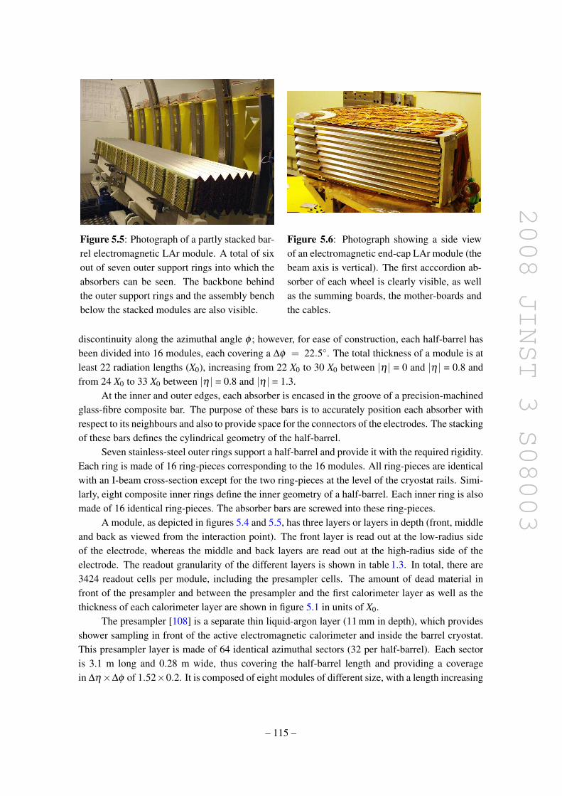
2008 JINST 3 S08003

Figure 5.5: Photograph of a partly stacked bar-rel electromagnetic LAr module. A total of sixout of seven outer support rings into which theabsorbers can be seen. The backbone behindthe outer support rings and the assembly benchbelow the stacked modules are also visible.

Figure 5.6: Photograph showing a side viewof an electromagnetic end-cap LAr module (thebeam axis is vertical). The first acccordion ab-sorber of each wheel is clearly visible, as wellas the summing boards, the mother-boards andthe cables.

discontinuity along the azimuthal angle φ ; however, for ease of construction, each half-barrel hasbeen divided into 16 modules, each covering a ∆φ = 22.5. The total thickness of a module is atleast 22 radiation lengths (X0), increasing from 22 X0 to 30 X0 between |η | = 0 and |η | = 0.8 andfrom 24 X0 to 33 X0 between |η | = 0.8 and |η | = 1.3.

At the inner and outer edges, each absorber is encased in the groove of a precision-machinedglass-fibre composite bar. The purpose of these bars is to accurately position each absorber withrespect to its neighbours and also to provide space for the connectors of the electrodes. The stackingof these bars defines the cylindrical geometry of the half-barrel.

Seven stainless-steel outer rings support a half-barrel and provide it with the required rigidity.Each ring is made of 16 ring-pieces corresponding to the 16 modules. All ring-pieces are identicalwith an I-beam cross-section except for the two ring-pieces at the level of the cryostat rails. Simi-larly, eight composite inner rings define the inner geometry of a half-barrel. Each inner ring is alsomade of 16 identical ring-pieces. The absorber bars are screwed into these ring-pieces.

A module, as depicted in figures 5.4 and 5.5, has three layers or layers in depth (front, middleand back as viewed from the interaction point). The front layer is read out at the low-radius sideof the electrode, whereas the middle and back layers are read out at the high-radius side of theelectrode. The readout granularity of the different layers is shown in table 1.3. In total, there are3424 readout cells per module, including the presampler cells. The amount of dead material infront of the presampler and between the presampler and the first calorimeter layer as well as thethickness of each calorimeter layer are shown in figure 5.1 in units of X0.

The presampler [108] is a separate thin liquid-argon layer (11 mm in depth), which providesshower sampling in front of the active electromagnetic calorimeter and inside the barrel cryostat.This presampler layer is made of 64 identical azimuthal sectors (32 per half-barrel). Each sectoris 3.1 m long and 0.28 m wide, thus covering the half-barrel length and providing a coveragein ∆η×∆φ of 1.52×0.2. It is composed of eight modules of different size, with a length increasing

– 115 –

2008 JINST 3 S08003

with |η | to obtain a constant η-granularity of ∆η = 0.2 for each module, except for the module atthe end of the barrel, for which the η-coverage is reduced to 0.12.

The presampler modules are made of interleaved cathode and anode electrodes glued betweenglass-fibre composite plates. The electrode spacing varies slightly, from 1.9 to 2.0 mm, with thepresampler module type. The cathodes are double-sided printed-circuit boards while the anodeshave three conductive layers separated by glass-fibre composite layers. The required segmentation,∆η ∼ 0.025 and ∆φ = 0.1, for each module is obtained by ganging the appropriate numberof anodes in the η direction and by subdividing (i.e. etching) each anode into two halves in theφ -direction. A high voltage potential of +2 kV is applied to the outer layers of the anodes and thesignal is read out through capacitive coupling to the central layer at ground potential.

5.2.3 End-cap geometry

The EMEC calorimeters [109] consist of two wheels, one on each side of the electromagnetic bar-rel. Each wheel is 63 cm thick and weighs 27 tonnes, with external and internal radii at ambienttemperature of 2098 mm and 330 mm, respectively. It covers the region 1.375 < |η | < 3.2. Inthe transition region between the barrel and the end-cap calorimeters, the material in front of thecalorimeter amounts to several X0, as shown in figure 5.1. In order to improve the energy measure-ment in this region, a liquid-argon presampler is implemented in front of the end-cap calorimeter,covering the range 1.5 < |η | < 1.8.

Each end-cap calorimeter consists itself of two co-axial wheels. The boundary between theinner and the outer wheel, which is 3 mm wide and located at |η | = 2.5, is mostly filled with low-density material. This boundary is approximately projective and matches the acceptance of theinner detector (see figure 4.1). Each end-cap wheel is further divided into eight wedge-shapedmodules without introducing any discontinuity along the azimuthal angle owing to the accordiongeometry. A view of a module is shown in figure 5.6. Each end-cap contains 768 absorbers in-terleaved with readout electrodes in the outer wheel and 256 absorbers in the inner wheel. Theelectrodes are positioned in the middle of the gaps by honeycomb spacers. The total active thick-ness of an end-cap calorimeter is greater than 24 X0 except for |η |< 1.475. The thickness increasesfrom 24 to 38 X0 as |η | increases from 1.475 to 2.5 (outer wheel) and from 26 to 36 X0 as |η | in-creases from 2.5 to 3.2 (inner wheel). The calorimeter support frame is composed of six supportrings: three on the front (at three different radii) and three on the back. The total weight of thedetector is supported mainly by the rings at the largest radius.

In the outer wheel, signals from the different pads are read out from both sides of the elec-trode, as in the case of the barrel electromagnetic calorimeter. In the inner wheel, because of thehigher radiation levels, the signals are all read out from the back side.

As for the barrel electromagnetic calorimeter, the precision region in the end-cap electromag-netic calorimeters (1.5 < |η | < 2.5) is divided in depth into three longitudinal layers. The frontlayer, about 4.4 X0 thick, is segmented with strips along the η direction. The transverse size of theprojective cell in the middle layer is the same as defined in the barrel electromagnetic calorimeter,∆η ×∆φ = 0.025×0.025. The back layer has a twice coarser granularity in η . The outermostregion |η | < 1.5 of the outer wheel and the inner wheel (2.5 < |η | < 3.2) are segmented inonly two longitudinal layers and have a coarser transverse granularity. Table 1.3 summarises the

– 116 –

2008 JINST 3 S08003

longitudinal and transverse readout granularities of the electromagnetic end-cap calorimeter as afunction of |η |. The η-granularity in the front layer varies with η in order to keep the copperstrip width larger than a few mm (see table 1.3). The φ -granularity is obtained by ganging thesignals from adjacent electrodes (see section 5.2.6). Each module contains 3984 readout channels,including the 96 channels in the presampler.

Each end-cap presampler consists of 32 identical azimuthal sectors or modules. These areplaced in a 5 mm deep cavity in the back of the cryostat cold wall. The granularity of the presam-pler is ∆η×∆φ = 0.025×0.1. One end-cap presampler module consists of two, 2 mm thick, activeliquid argon layers, formed by three electrodes parallel to the front face of the EMEC calorime-ter. The electrodes, made from double-sided printed-circuit boards, are separated by honeycombspacers and glued together at the inner and outer radius with 2 mm thick bars. A negative highvoltage is applied to the external electrodes and the signals are read out from the central electrodewhich is segmented into pads. The same signal, calibration and high-voltage cables as for theend-cap calorimeter are used. Two high-voltage cables feed separately the left and right side of apresampler module.

5.2.4 Shape and placement of the electromagnetic calorimeters

After insertion into the cryostat, the circularity of the barrel electromagnetic calorimeter was mea-sured. The deformation due to its weight can reach up to 3 mm at the top and bottom of eachhalf-barrel and is in fair agreement with the corresponding finite-element calculations [107]. In thecold, the deformation is reduced due to the Archimedes thrust caused by the liquid argon whichhas a relative density of 1.4. The centres of the fitted inner and outer circles coincide to betterthan 0.5 mm. Finally, the sagging of the absorbers was measured as a function of the azimuthalangle and a maximum value of 2.5 mm near the horizontal plane was found. The same set ofmeasurements has been performed for both end-caps, once they were in vertical position. Themeasured deformation was found to be up to 2 mm at the top. The sagging of the absorber platesand the small deformation of the barrel electromagnetic calorimeter will induce some distortions inthe position measurements but their impact on the energy resolution is expected to be very small.

Due to difficulties in the positioning of the half-barrels inside the cryostat, both half-barrelswhen cold are 4 mm too low and laterally displaced by 2 mm with respect to the cryostat axis[107]. Part of the vertical misalignment has been compensated by positioning the cryostat approx-imately 2 mm higher than originally planned inside the experiment (see section 9.3.2.3). To makeroom for the inner-detector services, the two end-cap cryostats have been positioned 40 mm awayfrom their nominal position in the z-direction. The projectivity of the geometry of these calorime-ters has therefore been slightly degraded.

5.2.5 High-voltage distribution

To provide a measure of redundancy, the two high-voltage sides of each electrode are fed inde-pendently. The nominal high-voltage for the barrel electromagnetic calorimeter is 2000 V (see ta-ble 5.1). If one side of an electrode is not powered, only half of the signal will be collected. Thevariation of the signal [110] with high voltage is mainly due to the variation of the drift velocity

– 117 –

2008 JINST 3 S08003

High voltage (kV)0 0.2 0.4 0.6 0.8 1 1.2 1.4 1.6 1.8 2 2.2

Tot

al e

nerg

y (G

eV)

0

50

100

150

200

250

245 GeV

100 GeV

Nominal HV

High voltage (kV)0.8 1 1.2 1.4 1.6 1.8 2 2.2 2.4

Tot

al e

nerg

y (G

eV)

100

120

140

160

180

200

Nominal HV

=1.7η

Figure 5.7: Measured electromagnetic cluster energy as a function of the applied high voltage. Theresults are shown for a barrel module (left), for 245 GeV electrons (open circles), 100 GeV elec-trons (open diamonds) and for the 100 GeV results at the nominal voltage of 2 kV scaled to thecorresponding result at 245 GeV (stars). The results obtained with an end-cap module (right) areshown for 193 GeV electrons. The curves correspond to fits with a functional form Etot = a×V b.

with high voltage and is shown in figure 5.7. The variation of the signal amplitude with high volt-age is moderate: for example, 77% of the signal is collected when decreasing the high voltage tohalf of its nominal value. The high-voltage granularity of the barrel electromagnetic calorimeter,including the presampler, is ∆φ ×∆η = 0.2×0.2, meaning that 32 electrode sectors are poweredsimultaneously.

η1.4 1.6 1.8 2 2.2 2.4 2.6 2.8 3 3.2

Hig

h vo

ltage

(kV

)

1

1.5

2

2.5

3

Figure 5.8: High-voltage distribution as a func-tion of |η | for the EMEC. A uniform calorime-ter response requires a high voltage which variescontinuously as a function of |η |, as shown by theopen circles. This has been approximated by a setof discrete values shown as full triangles.

In contrast to the barrel electromagneticcalorimeter, the drift gap on each side of theelectrodes is not constant for the EMEC, butis a function of radius and varies from 2.8 mmto 0.9 mm in the outer wheel and from 3.1 mmto 1.8 mm in the inner wheel. To obtain auniform η-independent detector response, onewould therefore need a high voltage contin-uously varying with η , as illustrated in fig-ure 5.8. In practice, this ideal behaviour is ap-proximated with a variation in steps, also il-lustrated in figure 5.8. Table 5.1 provides ex-plicitly these nominal high-voltage values asa function of the η-range, thereby definingseven (two) high-voltage sectors for the outer(inner) wheel. The high-voltage granularity isthus 0.2 in φ as in the barrel and approximately0.2 in η , as indicated in table 5.1.

Different solutions have been implemented in case of high-voltage problems. One electrodesector may be powered individually, if the problem was identified at room temperature. On theother hand, if the problem has been identified only in the cryostat when testing individual modules

– 118 –

2008 JINST 3 S08003

Table 5.1: Nominal high-voltage settings for the various liquid-argon calorimeter components andas a function of |η | in the case of the EMEC outer and inner wheels.

Component |η |-range and voltage (V)Electromagnetic barrel 0−1.475Voltage +2000Electromagnetic end-cap (EMEC) 1.375−1.5 1.5−1.6 1.6−1.8 1.8−2.0 2.0−2.1 2.1−2.3 2.3−2.5Voltage +2500 +2300 +2100 +1700 +1500 +1250 +1000Electromagnetic end-cap (EMEC) 2.5−2.8 2.8−3.2Voltage +2300 +1800Barrel presampler 0−1.52Voltage +2000End-cap presampler 1.5−1.8Voltage −2000Hadronic end-cap (HEC) 1.5−3.2Voltage +1800Forward calorimeter 3.1−4.9FCal1 voltage +250FCal2 voltage +375FCal3 voltage +500

at liquid-argon temperature, one high-voltage sector may be divided into two halves, for example∆φ ×∆η = 0.1× 0.2 in the barrel, and the two halves are powered separately. The effect of notsupplying high voltage at all to one side of the electrode was studied in the test-beam to verify theexpected factor of two loss in signal. A slight deviation from this expectation was observed forthe measured signal amplitude at the transition region with a good sector and this was understoodas a geometrical effect, which is easy to correct for since it is well reproduced by simulation. Analternative for sector sides with a permanent short is to supply them with high-voltage modulespermitting large DC current draws of up to 3 mA, which is in general sufficient to operate thefaulty sector at 1000 V or above.

5.2.6 Electronic boards and cables inside the cryostats

The first layer of each calorimeter is read out from the front (inner radius for the barrel electro-magnetic calorimeter and small-|z| face for the EMEC), whereas the second and third layers areread out from the back (outer radius for the barrel electromagnetic calorimeter and large-|z| facefor the EMEC). The readout is accomplished by several interconnected boards. These include sum-ming boards which generate analogue sums from adjacent calorimeter gaps and mother-boards foranalogue sum readout and for distribution of the calibration pulses.

The summing boards are connected to the electrode connectors grouping the signals in φ . Forthe barrel electromagnetic calorimeter and the outer EMEC wheel, each summing board servicesrespectively 16 and 12 electrodes (corresponding to ∆φ = 0.1). For the first layer, all electrodesare summed into one readout cell, while for the second and third layers they are summed in fouradjacent readout cells (∆φ = 0.025). For the inner EMEC wheel, each summing board serviceseight electrodes (∆φ = 0.2) and for each of the two layers, four adjacent electrodes are summed toform readout cells (∆φ = 0.1).

– 119 –

2008 JINST 3 S08003

A mother-board provides readout for a ∆η × ∆φ region of size 0.2×0.2. The receptaclesat the output of the summing boards and the input of the mother-boards are connected via pinsmounted on two thin printed-circuit boards. Each channel is connected twice to provide maximumrobustness and redundancy. For the second and third calorimeter layers, every other printed-circuitboard also houses a low-capacitance transient voltage suppressor [107], referenced to ground,with a turn-on at 6 V to protect against accidental discharges, which might damage the calibra-tion resistors mounted on the mother-board. The mother-boards route the outputs to the read-out cables through a connector designed to minimise cross-talk between readout channels. Themother-boards also include surface-mounted 0.1% tolerance tantalum-nitride calibration resistors(non-hygroscopic with a temperature coefficient of 70±5 ppm/C) to distribute calibration pulsesto all readout channels. The values of the calibration resistors in various parts of the detector arechosen to match the expected currents from particle showers [107, 109]. The calibration pulse isinjected at the analogue input to the mother-board, which is the point closest to the origin of theanalogue signals from the electrodes. Each presampler module is also equipped with a mother-board which collects signals from the readout cells and distributes the calibration pulses through aset of precision calibration resistors as mentioned above.

5.2.7 Quality-assurance tests

At each stage of the construction of the modules and assembly of the calorimeters, a number ofquality-assurance tests were carried out. The most important tests were those performed afterinsertion of the calorimeters inside their cryostats and after the first cool-down and liquid-argonfilling. All the signal and calibrations channels have been tested. Table 5.2 shows that the numberof missing or bad channels is below the specified acceptable number of faults.

A high-voltage test at the nominal settings was also performed at this stage. After this firstcold test, the calorimeters were heated back to room temperature before transportation and instal-lation in the ATLAS pit. High-voltage tests have also been performed on all calorimeters in theirfinal position in ATLAS. In the case of the barrel presampler and of the EMEC, most of the shortscan be eliminated by applying a high-voltage discharge [109, 111]. As a result, approximately 3%of the barrel electromagnetic channels and approximately 1% of the barrel and end-cap presamplerand EMEC channels remain with shorts, and therefore will be powered at a reduced voltage, asexplained in section 5.2.5.

5.3 Hadronic calorimeters

This section describes the ATLAS hadronic calorimeters: the tile calorimeter, the liquid-argonhadronic end-cap calorimeter (HEC) and the liquid-argon forward calorimeter (FCal).

5.3.1 Tile calorimeter

5.3.1.1 Overview

The tile calorimeter [105] is a sampling calorimeter using steel as the absorber and scintillatoras the active medium. It is located in the region, |η | < 1.7, behind the liquid argon electromag-netic calorimeter and is subdivided into a central barrel, 5.8 m in length, and two extended barrels,

– 120 –

2008 JINST 3 S08003

Table 5.2: Number of signal channels in each electromagnetic calorimeter layer and total numberof calibration channels, pre-defined acceptable maximum rate and maximum number of faults, andnumbers of faulty channels found after insertion at room temperature and later after cooling downand filling with liquid argon. Faulty channels correspond to either missing signal channels or signalchannels with a bad signal shape [107, 109].

Layer Number Maximum rate Maximum number Number of faulty channelsof of faults of faults accepted at room in liquid

channels accepted temperature argonElectromagnetic barrel calorimeter

Presampler 7808 0.05% 4 0 0Layer 1 57216 2 (per module) 64 9 11Layer 2 28672 0.05% 14 2 5Layer 3 13824 0.05% 6 0 4Barrel end 2048 0.05% 1 3 3Calibration 8192 0.05% 4 1 1

Electromagnetic end-cap calorimeterPresampler 1536 0.05% 1 0 1Layer 1 28544 2 (per module) 32 3 4Layer 2 23424 0.05% 12 2 7Layer 3 10240 0.05% 5 0 2Calibration 5952 0.05% 3 2 2

2.6 m in length and each having an inner radius of 2.28 m and an outer radius of 4.25 m, as shownin figure 1.3. The radial depth of the tile calorimeter is approximately 7.4λ (interaction lengths).Each barrel consists of 64 modules or wedges of size ∆φ ∼ 0.1, made of steel plates and scintillat-ing tiles [112].

The assembled module forms an almost-periodic steel-scintillator structure with a ratio byvolume of approximately 4.7:1. The geometry is sketched in figure 5.9. The orientation of thescintillator tiles radially and normal to the beam line, in combination with wavelength-shifting fibrereadout on the tile edges, allows for almost seamless azimuthal calorimeter coverage. The groupingof the readout fibres into the readout photomultiplier tubes (PMT’s) provides an approximatelyprojective geometry in pseudorapidity (see table 1.3). The gap region between the barrel and theextended barrel is instrumented with special modules, made of steel-scintillator sandwiches withthe same sampling fraction as the rest of the tile calorimeter and with thin scintillator countersin the sectors where the available space in the gaps is even more limited. These devices allow topartially recover the energy lost in the crack regions of the detector and are described in more detailin section 5.5.

The electronics and readout of the tile calorimeter are highly integrated with the mechanicalstructure. The photomultiplier tubes and all the front-end electronics are mounted in 1.4 m longaluminium units, called drawers, which are inserted inside the support girder at the rear of eachmodule (see section 5.6.1). The front-end electronics also provide analogue sums of subsets ofthe channels, forming trigger towers, for the L1 trigger (see section 5.6). The low-voltage power

– 121 –

2008 JINST 3 S08003

supplies which power the readout are mounted in an external steel box, which has the cross-sectionof the support girder and which also contains the external connections for power and other servicesfor the electronics (see section 5.6.3.1). Finally, the calorimeter is equipped with three calibrationsystems: charge injection, laser and a 137Cs radioactive source. These systems test the opticaland digitised signals at various stages and are used to set the PMT gains to a uniformity of ±3%(see section 5.6.2).

5.3.1.2 Mechanical structurePhotomultiplier

Wavelength-shifting fibre

Scintillator Steel

Source

tubes

Figure 5.9: Schematic showing how the mechan-ical assembly and the optical readout of the tilecalorimeter are integrated together. The vari-ous components of the optical readout, namelythe tiles, the fibres and the photomultipliers, areshown.

The mechanical structure of the tile calorime-ter is designed as a self-supporting, segmentedstructure comprising 64 modules, each sub-tending 5.625 degrees in azimuth, for each ofthe three sections of the calorimeter [112]. Themodule sub-assembly is shown in figure 5.10.Each module contains a precision-machinedstrong-back steel girder, the edges of whichare used to establish a module-to-module gapof 1.5 mm at the inner radius. To maximisethe use of radial space, the girder provides boththe volume in which the tile calorimeter read-out electronics are contained and the flux returnfor the solenoid field. The readout fibres, suit-ably bundled, penetrate the edges of the gird-ers through machined holes, into which plas-tic rings have been precisely mounted. Theserings are matched to the position of photomul-tipliers. The fundamental element of the ab-sorber structure consists of a 5 mm thick mas-ter plate, onto which 4 mm thick spacer platesare glued in a staggered fashion to form thepockets in which the scintillator tiles are lo-cated [113]. The master plate was fabricatedby high-precision die stamping to obtain the dimensional tolerances required to meet the specifica-tion for the module-to-module gap. At the module edges, the spacer plates are aligned into recessedslots, in which the readout fibres run. Holes in the master and spacer plates allow the insertion ofstainless-steel tubes for the radioactive source calibration system.

Each module is constructed by gluing the structures described above into sub-modules on acustom stacking fixture. These are then bolted onto the girder to form modules, with care beingtaken to ensure that the azimuthal alignment meets the specifications. The calorimeter is assembledby mounting and bolting modules to each other in sequence. Shims are inserted at the inner andouter radius load-bearing surfaces to control the overall geometry and yield a nominal module-to-module azimuthal gap of 1.5 mm and a radial envelope which is generally within 5 mm of thenominal one [112, 114].

– 122 –

2008 JINST 3 S08003

Master plate

Master plate

Scintillator tile

Wavelength−shifting fibre(decoupled from tile)

Wavelength−shifting fibre(viewing tile)

Plastic channel

Figure 5.10: Azimuthal view of the tile-calorimeter module-to-module interface show-ing the bearing locations at the inner and outerradii, and the azimuthal gap with a nominalwidth at the inner radius of 1.5 mm, in whichthe readout fibres are routed to the photomulti-pliers inside the girder.

Figure 5.11: Radial view, looking inwards to-wards the interaction point, showing the fibrerouting in the barrel modules. The fibre shownoutside the channel accepts light for the tileonto which it is pressed. Further along thechannel, this fibre is routed through a slot inthe channel, into the interior region, while oneof the other fibres is routed outside to view thenext series of scintillator tiles in depth.

5.3.1.3 Optical components

Eleven sizes of scintillating tiles (one for each depth in radius) of 3 mm thickness and with radiallengths ranging from 97 mm to 187 mm and azimuthal lengths ranging from 200 mm to 400 mmform the active medium of the tile calorimeter. Ionising particles crossing the tiles induce theproduction of ultraviolet scintillation light in the base material (polystyrene) and this light issubsequently converted to visible light by wavelength-shifting fluors (the polystyrene is dopedwith 1.5% PTP as the primary fluor and with 0.044% POPOP as the secondary fluor). Over460,000 scintillating tiles were produced for the tile calorimeter by injection molding of indi-vidual tiles: this eliminated the need for machining to form the trapezoidal shapes and drilling tocut the holes through which the calibration tubes must pass. The tolerance for all dimensions washeld to ± 0.10 mm. Approximately 5% of the tile production was tested with a 90Sr radioactivesource and the results were used to characterise the light output of each small group of approxi-mately twenty tiles in terms of maximum intensity and attenuation length [115]. Two sources ofraw polystyrene were used for tile fabrication; during assembly, the groups of tiles were sorted sothat tiles with similar response were inserted in contiguous areas of the detector.

Irradiation tests of tile/fibre assemblies indicated that in the first longitudinal sampling, for anintegrated dose corresponding to ten years of operation at the LHC design luminosity, a light lossof less than 10% is expected. Smaller losses will occur in the other samplings, where the radiationdose is less.

– 123 –

2008 JINST 3 S08003

Prior to insertion into the calorimeter, the tiles are inserted into a plastic sleeve, which bothprotects the tile and improves the scintillation light yield due to its high reflectivity of 95%. A maskpattern is printed on the sleeve to improve the optical uniformity. The resulting non-uniformity overthe surface of a tile is generally below 5% for the sum of signals on both sides of the tile.

Wavelength-shifting fibres placed in contact with the tile edges collect the scintillation lightproduced in the scintillators and convert it to a longer wavelength. Each fibre collects light fromtiles located at one or two radial depths in the calorimeter and transmits it to the PMT’s locatedinside the girder. The fibres used have a diameter of 1 mm, are equipped with a double cladding andare characterised by an emission peak at 476 nm with a decay time of∼ 6 ns. As part of the qualitycontrol, light output and attenuation were measured for sample fibres from each of the 65 pre-forms used for fibre production. The fibres have an attenuation length of 325 cm at a wavelengthof 430 nm, with a spread in attenuation length of ∼ 3% and in light output of ∼ 3% [116]. Toimprove the light output, the fibres are aluminised at the end opposite to the PMT. The aluminiummirrors were deposited using magnetron sputtering on bundles of 1261 fibres. The reflectivity wasrequired to be 75% and the spread of its variation is ∼ 7%, based on measurements from a sampleof fibres in each bundle [115]. The light output spread, at a fixed distance from the aluminised end,relative to a reference fibre, was found to be ∼ 3% for each fibre length [117].

To facilitate assembly, a novel approach was developed to manage the 540,000 fibres requiredto read out the scintillator tiles and form calorimeter cells. The fibres (four for the central barreland three for the extended barrel calorimeters) are inserted into a plastic channel much like a straw(see figures 5.9 and 5.11), which illustrate the scheme whereby depth segmentation is achieved inthe readout. The channels are opaque to avoid light cross talk, and painted with a high-reflectivityink on the side facing the tiles to maximise the light collection. Slots in the channels allow fibres topass from a location in which they face a tile to a location in which they do not, in order to decouplethe fibres at different depths in the calorimeter. The fibres were inserted in these channels using arobot [118] and are glued to the channel at a spot near the aluminised end of the fibre.

5.3.1.4 Instrumentation with scintillator and fibres

The light produced in the scintillating material is collected at the edges of each tile using twowavelength-shifting fibres as illustrated in figure 5.9. The fibres are grouped together and coupledto the PMT’s which are housed at the outer edge of each module. The fibre grouping is used todefine a three-dimensional cell structure in such a way as to form three radial sampling depths,approximately 1.5, 4.1 and 1.8 λ thick at η = 0. These cells have dimensions ∆η ×∆φ = 0.1×0.1 in the first two layers and 0.2× 0.1 in the last layer. The depth and η-segmentation of thebarrel and extended barrel modules are shown in figure 5.12. The fibres coupled to each edgeof the scintillating tiles are read out by two different PMT’s to provide redundancy and sufficientinformation to partially equalise signals produced by particles entering the scintillating tiles atdifferent impact positions.

Module instrumentation [119] comprised many steps, which ranged from cleaning the slots inthe absorber structure to a set of final module quality-control measurements based on the individualtile fibre response. Following insertion of tiles and channel/fibre assemblies into a module, thefibres are grouped together to form cells and are glued as a bundle into the fibre-insertion tube, as

– 124 –

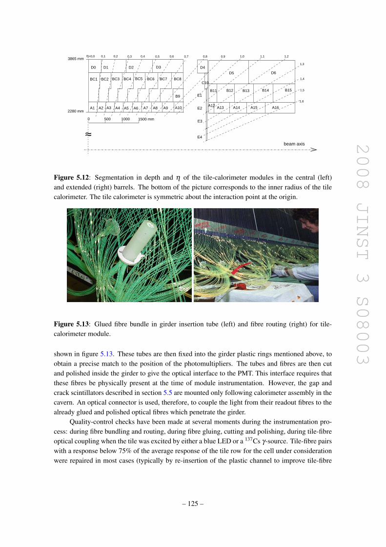
2008 JINST 3 S08003

500 1000 1500 mm0

A3 A4 A5 A6 A7 A8 A9 A10A1 A2

BC1 BC2 BC3 BC5 BC6 BC7 BC8BC4

D0 D1 D2 D3

A13 A14 A15 A16

B9

B12 B14 B15

D5 D6D4

C10

0,7 1,0 1,1

1,3

1,4

1,5

1,6

B11 B13

A12

E4

E3

E2

E1

beam axis

0,1 0,2 0,3 0,4 0,5 0,6 0,8 0,9 1,2

2280 mm

3865 mm=0,0η

~~

Figure 5.12: Segmentation in depth and η of the tile-calorimeter modules in the central (left)and extended (right) barrels. The bottom of the picture corresponds to the inner radius of the tilecalorimeter. The tile calorimeter is symmetric about the interaction point at the origin.

Figure 5.13: Glued fibre bundle in girder insertion tube (left) and fibre routing (right) for tile-calorimeter module.

shown in figure 5.13. These tubes are then fixed into the girder plastic rings mentioned above, toobtain a precise match to the position of the photomultipliers. The tubes and fibres are then cutand polished inside the girder to give the optical interface to the PMT. This interface requires thatthese fibres be physically present at the time of module instrumentation. However, the gap andcrack scintillators described in section 5.5 are mounted only following calorimeter assembly in thecavern. An optical connector is used, therefore, to couple the light from their readout fibres to thealready glued and polished optical fibres which penetrate the girder.

Quality-control checks have been made at several moments during the instrumentation pro-cess: during fibre bundling and routing, during fibre gluing, cutting and polishing, during tile-fibreoptical coupling when the tile was excited by either a blue LED or a 137Cs γ-source. Tile-fibre pairswith a response below 75% of the average response of the tile row for the cell under considerationwere repaired in most cases (typically by re-insertion of the plastic channel to improve tile-fibre

– 125 –

2008 JINST 3 S08003

optical coupling or replacement of the fibre). The average cell response uniformity for produc-tion modules, measured using the caesium source, is shown in figure 5.14 and meets the designspecification of 10%.

5.3.2 Hadronic end-cap calorimeters (HEC)

5.3.2.1 Overview

0.04

0.06

0.08

0.1

0 10 20 30 40 50 60Production module number

Uni

form

ity Tile barrel

0.04

0.06

0.08

0.1

0 10 20 30 40 50 60Production module number

Uni

form

ity Tile extended barrel (side C)

0.04

0.06

0.08

0.1

0 10 20 30 40 50 60Production module number

Uni

form

ity Tile extended barrel (side A)

Figure 5.14: Average cell response uniformity,measured using the caesium calibration systemfor the barrel and the two extended barrel tilecalorimeters.

Figure 5.15 shows a schematic view ofthe design of a HEC module.The hadronicend-cap calorimeter (HEC) [104, 120] isa copper/liquid-argon sampling calorimeterwith a flat-plate design, which covers therange 1.5 < |η | < 3.2. The HEC shares eachof the two liquid-argon end-cap cryostats withthe electromagnetic end-cap (EMEC) and for-ward (FCal) calorimeters (see figure 5.25). TheHEC consists of two wheels in each end-capcryostat: a front wheel (HEC1) and a rearwheel (HEC2), each wheel containing two lon-gitudinal sections. The wheels are cylindricalwith an outer radius of 2030 mm. Each of thefour HEC wheels is constructed of 32 identi-cal wedge-shaped modules, as illustrated in fig-ure 5.16. A stainless-steel connecting-bar sys-tem at the outer wheel perimeter guarantees themechanical integrity of the wheel structure. Atthe inner radius, small copper connecting bars link the plates of each set of neighbouring modules.Two sliding rails support the wheels inside the cryostat and are an integral part of the mechanicalstructure. The final vertical deformation of the wheel structure has been measured for the fourwheels to represent a sag of 0.3 mm on average. The wheels remain perpendicular to their axiswithin ±1.0 mm.

The modules of the front wheels are made of 24 copper plates, each 25 mm thick, plus a12.5 mm thick front plate. In the rear wheels, the sampling fraction is coarser with modules madeof 16 copper plates, each 50 mm thick, plus a 25 mm thick front plate. The gaps in between theplates all have a thickness of 8.5 mm. The resulting sampling fractions for HEC1 and for HEC2are 4.4% and 2.2% respectively. The wheels have an inner radius of 372 mm for the first nine platesof HEC1 and of 475 mm for the remaining plates of HEC1 and for all 17 plates of HEC2. Thestructural strength of the modules is provided by seven stainless-steel tie-rods with 12 mm (16 mm)diameter for the front (rear) modules. Annular high-precision spacers on the tie-rods maintain the8.5 mm gaps between the copper plates.

Three electrodes divide the 8.5 mm gaps into four separate LAr drift zones of 1.8 mm widtheach. Figure 5.17 shows schematically the arrangement of the readout structure. The space betweenthe electrodes is maintained using a honeycomb sheet which is also held in place by the seven

– 126 –

2008 JINST 3 S08003

Figure 5.15: Schematic R− φ (left) and R− z (right) views of the hadronic end-cap calorimeter.The semi-pointing layout of the readout electrodes is indicated by the dashed lines. Dimensionsare in mm.

tie-rods. Each drift zone is individually supplied with high voltage (see table 5.1). The middleelectrode carries a pad structure covered by a high-resistivity layer, serving as the readout electrodeand defining the lateral segmentation of the calorimeter. The two other electrodes carry surfaces ofhigh resistivity to which high voltage is applied. These high-voltage planes form an electrostatictransformer (EST). Electrically, this structure corresponds to a double gap of 3.6 mm each. TheEST structure has the advantage of a lower high-voltage for operation, of a double high-voltagesafety and thus of reduced problems with space-charge effects due to ion density at large valuesof |η |. For the nominal high voltage of 1800 V, the typical drift time for electrons in the drift zoneis 430 ns.

The readout cells are defined by pads etched on the central foil in each gap. The arrangementof these pads provides a semi-pointing geometry (see figure 5.15). The size of the readout cells is∆η×∆φ = 0.1×0.1 in the region |η | < 2.5 and 0.2×0.2 for larger values of η .

The signals from the pads of this electrode structure are amplified and summed employingthe concept of active pads [121]: the signals from two consecutive pads are fed into a separatepreamplifier (based on GaAs electronics). The use of GaAs preamplifiers in the cold provides the

– 127 –

2008 JINST 3 S08003

Figure 5.16: Schematic view of a HEC mod-ule, with a cut-away showing the readout struc-ture and the active-pad electronics.

Figure 5.17: Schematic of the arrangement ofthe HEC readout structure in the 8.5 mm inter-plate gap. All dimensions are in mm.

optimum signal-to-noise ratio for the HEC. An important aspect of the HEC is its ability to detectmuons and to measure any radiative energy loss. The density of the electronics on the HEC wheelswith their rather modest number of read-out channels (5632 in total) and the power consumption ofthe GaAs integrated circuits (15 mW for one preamplifier channel and approximately 200 mW forthe entire chip) are sufficiently low that the heating effect of the electronics on the liquid argon doesnot produce bubbling. The outputs of the preamplifiers are summed on the same GaAs integratedcircuit to produce one signal from each cell. The signal sent to the feed-through for each cell isthus comprised of the amplified and summed signals of the eight or sixteen pads with the same η

and φ within a readout section.

5.3.2.2 Wheel assembly and installation

Figure 5.18 shows a HEC wheel fully assembled on its assembly table. The geometrical precisionof the wheel is given by 32 datum pins on the assembly table. During the wheel assembly, eachmodule had to pass a series of quality-assurance tests: high-voltage reliability, capacitance control,electronic cabling and signal reconstruction verification using the calibration procedures in warmand in cold. These tests were repeated after the wheel assembly, after the wheel rotation, after thewheel insertion, after the full cabling of the HEC1 and HEC2 wheels inside the cryostat and finallythrough the feed-throughs of the cryostat.

After closing the end-cap cryostat, each end-cap has been cooled down, filled with LAr andthe final cold tests prior to the movement to the ATLAS cavern have been performed. For the HEC,

– 128 –

2008 JINST 3 S08003

Figure 5.18: Photograph of a fully assembled HEC wheel on the assembly table. The active-padelectronic boards located on the outer circumference are clearly visible.

these tests included quality-assurance measurements and cabling checks of all signal and calibra-tion lines, full calibration and delay scans of all signal channels, full pulse-shape analysis of allsignal channels, detailed noise measurements of all channels including coherent noise and a long-term high-voltage test of all high-voltage lines. Typically, three signal channels per end-cap werefound to be not fully operational, corresponding to 0.1 % of all channels, as shown in table 5.3.The fraction of high-voltage lines with shorts was ∼ 4 % in liquid argon, but, most importantly,with four individual high-voltage lines per individual HEC gap, all HEC regions are operational(see also table 5.1 which lists the nominal high-voltage settings for the HEC).

5.3.3 Forward calorimeters

5.3.3.1 Overview

The forward calorimeters (FCal) are located in the same cryostats as the end-cap calorimeters andprovide coverage over 3.1 < |η | < 4.9. The close vicinity and coupling between these systemsresult in a quite hermetic design, which minimises energy losses in cracks between the calorimetersystems and also limits the backgrounds which reach the muon system. As the FCal modules arelocated at high η , at a distance of approximately 4.7 m from the interaction point, they are exposed

– 129 –

2008 JINST 3 S08003

Table 5.3: Table showing the number of faulty signal channels in each segment and the num-ber of faulty calibration lines for both hadronic end-caps after insertion at room temperature andafterwards in liquid argon.

HEC module and Total number Number of faulty Number of faulty Percentagesection of channels channels (ambient) channels (in liquid) (%)HEC1 (first section) 1536 0 0 0HEC1 (second section) 1472 0 3 0.20HEC2 (first section) 1344 0 0 0HEC2 (second section) 1280 1 2 0.16Calibration 1024 1 1 0.1

Table 5.4: Table of parameters for the three FCal modules.FCal1 FCal2 FCal3

Function Electromagnetic Hadronic HadronicMass of module (kg) 2119 3826 3695Main absorber material Copper Tungsten TungstenLAr gap width (mm) 0.269 0.376 0.508Radiation length (X0) 27.6 91.3 89.2Absorption length (λ ) 2.66 3.68 3.60Number of electrodes 12260 10200 8224Number of readout channels 1008 500 254

to high particle fluxes. This has resulted in a design with very small liquid-argon gaps, which havebeen obtained by using an electrode structure of small-diameter rods, centred in tubes which areoriented parallel to the beam direction. The liquid-argon gaps are smaller than the usual 2 mm gapof the electromagnetic barrel calorimeter to avoid ion build-up problems and to provide at the sametime the highest possible density. These smaller gaps also lead to a faster signal with roughly thesame instantaneous current but smaller integrated current. In the electromagnetic layer (FCal1),the triangular current pulse at the electrode has a full drift time of 60 ns. For FCal2 and FCal3, thefull drift time scales with the gap size since the field in the gaps is similar for all three modules.

5.3.3.2 Module description

Each FCal is split into three 45 cm deep modules: one electromagnetic module (FCal1) and twohadronic modules (FCal2 and FCal3), as illustrated in figure 5.19. To optimise the resolution andthe heat removal, copper was chosen as the absorber for FCal1, while mainly tungsten was usedin FCal2 and FCal3, to provide containment and minimise the lateral spread of hadronic showers.A shielding plug made of a copper alloy has been mounted behind FCal3 to reduce backgrounds inthe end-cap muon system. A full description of the FCal detector can be found in [122].

The basic parameters of the FCal modules are listed in table 5.4. The FCal1 layer is made ofcopper plates stacked one behind the other. The plates have 12,260 holes drilled in them throughwhich the electrode structures are inserted. An electrode consists of a co-axial copper rod and

– 130 –

2008 JINST 3 S08003

450 550500400350 600 650

60

50

40

30

20

10

0

R (

cm)

z (cm)

EMEC

HEC(back)

Pump

FCal 1 FCal 2 FCal 3

(EM) (Had) (Had)

(front)HEC

Moderator shielding shiel

ding p

lug

LAr Calo

rimete

r R

LAr gap

Beam-pipe

Warmwall

Super-insulationColdwall

Figure 5.19: Schematic diagram showing thethree FCal modules located in the end-capcryostat. The material in front of the FCal andthe shielding plug behind it are also shown.The black regions are structural parts of thecryostat. The diagram has a larger verticalscale for clarity.

Figure 5.20: Electrode structure of FCal1 withthe matrix of copper plates and the copper tubesand rods with the LAr gap for the electrodes.The Molière radius, RM, is represented by thesolid disk.

copper tube separated by a precision, radiation-hard plastic fibre wound around the rod. The ar-rangement of electrodes and the effective Molière radius for the modules can be seen in figure 5.20.Mechanical integrity is achieved by a set of four tie-rods which are bolted through the structure.The electrode tubes are swaged at the signal end to provide a good electrical contact.

The hadronic modules FCal2 and FCal3 are optimised for a high absorption length. Thisis achieved by maximising the amount of tungsten in the modules. These modules consist oftwo copper end-plates, each 2.35 cm thick, which are spanned by electrode structures, similar tothe ones used in FCal1, except for the use of tungsten rods instead of copper rods. Swaging ofthe copper tubes to the end-plates is used to provide rigidity for the overall structure and goodelectrical contact. The space between the end-plates and the tubes is filled with small tungstenslugs, as shown in figure 5.21. The inner and outer radii of the absorber structure formed by therods, tubes and slugs are enclosed in copper shells.

Signals are read out from the side of FCal1 nearer to the interaction point and from thesides of FCal2 and FCal3 farther from the interaction point. This arrangement keeps the cablesand connectors away from the region of maximum radiation damage which is near the back ofFCal1. Readout electrodes are hard-wired together with small interconnect boards on the facesof the modules in groups of four, six and nine for FCal1, FCal2 and FCal3 respectively. Thesignals are then routed using miniature polyimide co-axial cables along the periphery of the FCalmodules to summing boards which are mounted on the back of the HEC calorimeter. The summingboards are equipped with transmission-line transformers which sum four inputs. High voltage(see table 5.1) is also distributed on the summing boards via a set of current-limiting resistors, asshown in figure 5.22 for the specific case of FCal1. The signal summings at the inner and outerradii of the modules are in general different due to geometric constraints and higher counting ratesat the inner radius [122].

– 131 –

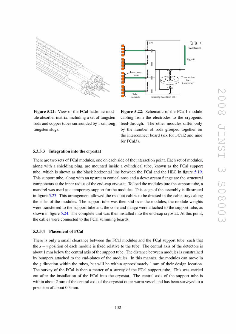
2008 JINST 3 S08003

Tube

electrode Summing board unit cell

HV

Pig-tail

Feed-through

Transmission

line

transformer

Interconnect

board

Figure 5.21: View of the FCal hadronic mod-ule absorber matrix, including a set of tungstenrods and copper tubes surrounded by 1 cm longtungsten slugs.

Figure 5.22: Schematic of the FCal1 modulecabling from the electrodes to the cryogenicfeed-through. The other modules differ onlyby the number of rods grouped together onthe interconnect board (six for FCal2 and ninefor FCal3).

5.3.3.3 Integration into the cryostat

There are two sets of FCal modules, one on each side of the interaction point. Each set of modules,along with a shielding plug, are mounted inside a cylindrical tube, known as the FCal supporttube, which is shown as the black horizontal line between the FCal and the HEC in figure 5.19.This support tube, along with an upstream conical nose and a downstream flange are the structuralcomponents at the inner radius of the end-cap cryostat. To load the modules into the support tube, amandrel was used as a temporary support for the modules. This stage of the assembly is illustratedin figure 5.23. This arrangement allowed the readout cables to be dressed in the cable trays alongthe sides of the modules. The support tube was then slid over the modules, the module weightswere transferred to the support tube and the cone and flange were attached to the support tube, asshown in figure 5.24. The complete unit was then installed into the end-cap cryostat. At this point,the cables were connected to the FCal summing boards.

5.3.3.4 Placement of FCal

There is only a small clearance between the FCal modules and the FCal support tube, such thatthe x− y position of each module is fixed relative to the tube. The central axis of the detectors isabout 1 mm below the central axis of the support tube. The distance between modules is constrainedby bumpers attached to the end-plates of the modules. In this manner, the modules can move inthe z direction within the tubes, but will be within approximately 1 mm of their design location.The survey of the FCal is then a matter of a survey of the FCal support tube. This was carriedout after the installation of the FCal into the cryostat. The central axis of the support tube iswithin about 2 mm of the central axis of the cryostat outer warm vessel and has been surveyed to aprecision of about 0.3 mm.

– 132 –

2008 JINST 3 S08003

Figure 5.23: Assembly of FCal modules: fromleft to right, the three modules plus the copperalloy plug can be seen on the support mandrelwith most of the cabling in place.

Figure 5.24: Completed FCal assembly withits bulkhead and cone attached, just before in-sertion into the end-cap cryostat.

5.3.3.5 Tests during installation/integration

A series of quality-control checks were carried out on the modules. These included high-voltagetesting, capacitance measurements and reflection testing. The results of the capacitance measure-ments provided a measure of the uniformity of the electrodes. High-voltage checks were carriedout at each stage of assembly and integration of the detectors both at warm and at cold. It wasfound that the number of shorts did vary during this process. The reflection tests were used to lookfor other detector faults, such as disconnected channels and broken ground braids.

A summary of the faults observed in the FCal modules after the cryostats were installed inthe ATLAS cavern and filled with liquid argon can be found in table 5.5. The right-hand columnshows the number of readout channels per module which have a fault leading to a distorted signal,a reduction in signal amplitude or to both of these effects. It is expected that the output fromthese channels can be adjusted in the signal reconstruction to partially recover the true amplitude,including when the fault arises from high-voltage problems. The 1762 channels in each FCal areserved by 112 high-voltage lines. Two of these were lost during the FCal integration into the end-cap cryostat, one for FCal1 on side C and the other for FCal3 on side A. This accounts for thelarge number of faulty channels shown for these two modules in table 5.5. There are sixteen high-voltage shorts on the FCal on side A and nine on side C. These account for roughly half of theremaining faults listed in table 5.5. The other half are dominated by damaged blocking capacitors(see figure 5.22). A more detailed description of the faults observed in the modules can be foundin ref. [122].

– 133 –

2008 JINST 3 S08003

Table 5.5: Summary of faults found in the FCal modules after installation in ATLAS. Shown foreach module are the total number of channels, the number of dead channels and the number offaulty channels which will require special treatment in the reconstruction of the signal (see text).Faulty channels correspond to either missing signal channels or signal channels with a bad signalshape [122].

ChannelsModule Total number Number Number

of channels of dead channels of faulty channelsFCal1 (side A) 1008 0 26FCal2 (side A) 500 1 4FCal3 (side A) 254 1 59

FCal1 (side C) 1008 5 51FCal2 (side C) 500 0 8FCal3 (side C) 254 1 4

5.4 Cryostats and associated feed-throughs

5.4.1 Cryostat description

As mentioned above, the liquid-argon calorimeters are located in three different cryostats. Fig-ure 1.3 shows the general features and location of the barrel and end-cap cryostats in the overallcalorimeter system. Each cryostat is composed of two concentric aluminium vessels, an inner coldvessel and an outer warm vessel. Each vessel forms a cylindrical torus centred on the beam axisand the space in between the vessels is under vacuum. As described in section 2.1.1, the centralsolenoid is housed in the insulating vacuum of the barrel cryostat and supported by the inner cylin-der of the warm barrel vessel. The two end-cap cryostats each house one electromagnetic end-capcalorimeter (EMEC), one hadronic end-cap calorimeter (HEC) and one forward calorimeter (FCal).Figure 5.25 shows a more detailed cut-away view of one end-cap cryostat with the three differentcalorimeter systems it contains.

The different vessels are closed at both ends by bulkheads. All bulkheads are circular-shapedplates with passage holes. The barrel passage holes allow the insertion of the inner detector andof its associated beam-pipe into the inner warm vessel bore. The end-cap passage holes allowthe passage of the next section of the beam-pipe and the insertion of its associated pump station(see section 9.8). The barrel bulkheads and the inner cold vessel of the barrel cryostat have taperedwalls to minimise the material and dead space between the interaction region and the electromag-netic calorimeters. To further minimise the amount of material, the cold and warm front end-capbulkheads are flat, and insulating spacers allow the warm bulkhead to sit on the cold one.

The cold vessels rest on four feet made of a glass-fibre composite material, which provideelectrical and thermal insulation to the warm vessels. The barrel cryostat load is transferred directlyto the ATLAS main rail system through the tile-calorimeter support saddles. For the support on

– 134 –

2008 JINST 3 S08003

Electromagnetic end-cap calorimeter

Forward calorimeter

Feed-throughs and front-end crates

Hadronic end-cap calorimeter

Figure 5.25: Cut-away view of an end-cap cryostat showing the positions of the three end-capcalorimeters. The outer radius of the cylindrical cryostat vessel is 2.25 m and the length of thecryostat is 3.17 m.

the side of the end-cap cryostat pointing towards the interaction point, this is not possible and theload is transferred through the inner radius of the extended calorimeter on a vertically adjustablesupport.

5.4.2 Signal feed-throughs

The signal feed-throughs bring all the signal, monitoring, calibration and spare lines through theinsulating vacuum from the liquid-argon cold volume to the front-end crates located at room tem-perature around and on the outside of the barrel and end-cap cryostats. A total of 64 feed-throughsserve the 122,800 lines of the barrel electromagnetic calorimeter, whereas a total of 2× 25 feed-throughs serve the 2× 48,000 lines of the two end-caps. In each end-cap, 20 feed-throughs areused by the EMEC, four by the HEC and one by the FCal (the EMEC uses also part of the fourHEC feed-throughs).

A feed-through [123] consists primarily of a warm flange and a cold flange, with a flexiblebellows welded between them. The volume between the two flanges is under vacuum. Each flangehouses four gold-plated pin carriers, providing a total of 1920 signal connections per feed-through.

– 135 –

2008 JINST 3 S08003

Both pin carriers are interconnected with flat polyimide strip-line flexible cables. To minimise thelengths of the connection lines, the signal feed-throughs are distributed radially around each end ofthe barrel cryostat and at the back of each of the end-cap cryostats.

5.4.3 High-voltage feed-throughs

Two high-voltage feed-through ports [124] are mounted on each cryostat. They are located closeto the highest point at each end of the barrel cryostat and at the back of each end-cap cryostat. Aport consists of a single warm bulkhead mounted on the warm vessel, from which the wire bundleleads to the calorimeter via a tube connected to the cold vessel by stainless-steel bellows. Theliquid argon rises up to the bellows and is followed, instead of vacuum, by a 70 cm high columnof argon gas at 1.25 bar. With such an arrangement, the HV wires are never under vacuum andthus not subject to corona effects. The high-voltage wire consists of a solid 0.41 mm diameterconstantan (Cu/Ni alloy) conductor with a 0.30 mm thick radiation-hard plastic (polyether-ether-ketone) cladding. Each port holds approximately 840 HV lines. These lines serve the standardhigh-voltage lines and the spares may be used to supply single electrodes or split sectors which donot hold the nominal high voltage (see section 5.2.5).

5.5 Instrumentation in gap between cryostats

The transition region or gap between the barrel and end-cap calorimeters is filled with cables andservices for the inner detector as well as power supplies and services for the barrel liquid-argoncalorimeter. One of the standard gap regions is shown in figures 5.12 and 5.26. At the outer radiusof the detector, a reduced section of a standard tile-calorimeter sub-module, the plug, providesadditional coverage in this region and significantly reduces the neutron flux from the inner-detectorvolume into the muon system.

In the region of the tile-calorimeter module where part of the calorimeter structure has beenremoved, two scintillators (E1 and E2 shown in figure 5.12) with independent readout (the gap scin-tillators) are attached to the module surface. The gap scintillators cover the region 1.0 < |η | < 1.2and provide signals which can be used to correct for energy losses in the inactive material in the gap.

Two scintillators (E3 and E4 shown in figure 5.12), the cryostat scintillators, penetrate theregion between the outer walls of the barrel and end-cap cryostats. These are physically attachedto the tile calorimeter and read out through its electronics. The cryostat scintillators cover theregion 1.2 < |η | < 1.6 and provide a signal which can be used to correct for energy losses in theouter wall of the barrel cryostat and in the inner-detector services. Both gap and crack scintillatorshave full coverage in φ , with a segmentation of ∆φ = 0.1.

For initial data-taking at low luminosities, two sets of sixteen scintillator counters installedon the front face of the end-cap calorimeter cryostats will be used to trigger on minimum-biasevents. Each set of counters is segmented in eight units in φ and two units in η . They are locatedat |z| = 3560 mm, the innermost set covers radii between 153 mm and 426 mm, corresponding tothe region 2.82 < |η | < 3.84 and the outermost set covers radii between 426 mm and 890 mm,corresponding to the region 2.09 < |η | < 2.82. The readout for these counters will be providedby that of sixteen of the cryostat scintillators covering the region 1.2 < |η | < 1.4. Eight of

– 136 –

2008 JINST 3 S08003

Figure 5.26: Schematic of the transition region between the barrel and end-cap cryostats, whereadditional scintillator elements are installed to provide corrections for energy lost in inactive ma-terial (not shown), such as the liquid-argon cryostats and the inner-detector services. The plugtile calorimeter is fully integrated into the extended barrel tile calorimeter. The gap and cryostatscintillators are read out together with the other tile-calorimeter channels (see text).

these cryostat scintillators had to be removed on each side for the routing of the signals from theminimum-bias scintillators. They will be reinserted for operations at full luminosity.

There are several locations around the circumference of the calorimeter, in which the standardgap instrumentation is not possible, for example the region opposite the support feet for the barrelcryostat [112]. In these locations, the plug calorimeter is reduced further in its length. In thelocation of the exit of the barrel cryogenic line, no plug calorimeter can be accommodated and it isreplaced entirely by scintillators. Finally, the inner support of the end-cap cryostat sits on the tilecalorimeter at its inner radius. In these regions, the tile-calorimeter modules themselves are cut toprovide the support surface on which the cryostat support jacks sit. The gap scintillators are alsomissing in this region.

5.6 Calorimeter readout electronics, calibration and services

5.6.1 Readout electronics

5.6.1.1 Overview

This section describes the on-detector (front-end) and off-detector (back-end) electronics of theATLAS calorimetry. The major tasks required of the readout electronics are to provide the first-level (L1) trigger system with the energy deposited in trigger towers of size ∆η ×∆φ = 0.1×0.1and to measure, for L1-triggered beam crossings, the energy deposit in each calorimeter cell to the

– 137 –

2008 JINST 3 S08003

|η|0 0.5 1 1.5 2 2.5 3 3.5 4 4.5 5E

lect

roni

c no

ise

at z

ero

lum

inos

ity (

MeV

)

210

310

FCal1

FCal2

FCal3

HEC1

HEC2

HEC3

HEC4

PS

EM1

EM2

EM3

Tile1

Tile2

Tile3

Figure 5.27: Expected electronic noise in individual cells of the various sampling layers of thecalorimeters as a function of |η |. Note that the presampler noise is corrected for by the appropriatesampling fractions as discussed in section 5.6.2.1.

specifications set by the performance requirements. The dynamic range to be covered ranges froma maximum of 3 TeV down to a lower limit of ∼ 10 MeV set by thermal noise in the calorime-ters. The thermal noise from the front-end electronics varies widely across the various calorimetersystems, as illustrated in figure 5.27. Coherent noise over the many cells used to measure elec-tron/photon energies in the electromagnetic calorimeters and jet energies and Emiss

T in the overallcalorimetry should be kept below 5% of the incoherent noise. The readout should proceed withoutany appreciable dead-time up to a trigger rate of 75 kHz.

As already described for the overall experiment in section 3.1, all electronics componentssituated in the cavern have to be radiation-tolerant to specifications including large safety fac-tors. However, the necessity for a large dynamic range and for very low coherent noise favoursa readout architecture with analogue processing very close to the detectors. These quite stringentrequirements have led to solutions where the analogue signals are amplified, processed and digi-tised by radiation-tolerant front-end electronics mounted very near the detectors (just above thesignal feed-throughs for the LAr calorimeters and in drawers incorporated into the girders for thetile calorimeters) and followed by subsequent digital processing of the signals in back-end systemswhich are located off-detector. For example, the overall readout architecture of the LAr calorime-ters is sketched out in figure 5.28. This overall electronics readout system [125, 126] is used forall the LAr calorimeters and, as shown in figure 5.28, provides also the necessary input for theL1 calorimeter trigger (see section 8.2).

– 138 –

2008 JINST 3 S08003

TT

C v

i + T

TC

ex

LTP

CP

U

CP

U

SP

AC

ma

ste

r b

oa

rd

ROD

TB

M b

oa

rd

E= ∑ai S

i

T= ∑bi S

i

CTP

External triggers

L1

processor

L1

interface Calorimeter

monitoring

Rc

Lc

DAC

Clock

I

∑

∑

Optical link

Controller

Optical

reception

SPAC

slave

Preamplifiers

Buffering

&

ADC

SPAC slaveSPAC slave SPAC slave

Calibration Tower builder

Controller

board

Front-end board

Front-end crate

TTCrx

40 MHz clock

L1A

SPAC bus

TTC crate

Readout crate (ROC)

32 bits

40 MHz

US

A1

5O

n d

ete

cto

r

Cryostat

SC

A

La

ye

r S

um

~1

5k

~1

80

k

Mother-board

Electrode

T=90°K

networkDAQ

Sh

ap

ers

∫ ∫ ∫

Cd

Figure 5.28: Block diagram depicting the architecture of the overall LAr readout electronics. Thelower box depicts the cold electrical circuit in the calorimeter cryostat. The central box illustratesthe functionality of the front-end boards located in the on-detector front-end electronics crateswhich are mounted on the cryostat feed-throughs. The upper layer shows the off-detector back-endelectronics components (ROD boards and TTC modules) mounted in their readout crates, togetherwith the LAr front-end tower builder electronics and the interfaces to the L1 trigger system with itscentral trigger processor (CTP).

– 139 –

2008 JINST 3 S08003

The radiation levels in the vicinity of the LAr cryostats and tile drawers (fluences of 1012 neu-trons per cm2 per year and ionising doses of 20 Gy per year) have required the development anduse of a large number of specifically designed radiation-hard ASIC’s for many key components ofthe front-end electronics of the calorimeters. The back-end systems, located in the main servicescavern (USA15), where there are no radiation issues, use commercial components. The back-endelectronics systems for all LAr calorimeters and for the tile calorimeter have been designed withthe same architecture, although some important differences exist in the functional implementation.

As discussed in section 9.4.8, an important effort has been invested in implementing thegrounding and electromagnetic compatibility rules for ATLAS during the design and installationphases of the calorimeters and of their electronics. This has been particularly demanding for theLAr cryostats, since all services, such as cryogenic lines, cooling pipes, etc., and all mechanicalconnections to the surrounding detector systems had to be installed in a way which preservedthe electrical isolation of the cryostats. The most difficult challenge has been related to the largeamount of pipes which run along the cryostat walls and enter the inner bore of the barrel cryostat toservice the inner detector. The cryostat surfaces are wrapped in insulating foils or covered by thinglass-fibre sheets to prevent any accidental electrical contact. Concerning the calorimeter electricalconnections, the DC isolation of the power to the front-end boards is taken care of by the DC-DC converters of the low-voltage power supplies (see section 5.6.3.1). The shields of all cablesconnected to the cryostats are interrupted at one end. For example, the shield of the L1 cables(the only copper links in the calorimeter readout) is disconnected at the entrance of the receiverboards. The cryostats themselves are connected to the safety ground [127] by long cables with alarge copper cross-section to a single point close to the L1 receiver racks. This choice minimisesthe potential difference between the analogue sending and receiving ends of the trigger signals.The tile calorimeter itself is structurally supported on rails which are grounded to the cavern safetynetwork. Additionally, dedicated grounding cable connections for each of the three tile calorimeterbarrels are made to the cavern network [128].

5.6.1.2 LAr calorimeter front-end electronics

The sensitive analogue electronics [125] are located on the detector. Inside the cryostat, thecalorimeter electrodes are grouped to form readout cells and small coaxial cables bring the cellsignals to the cold-to-warm feed-throughs (see section 5.4), except for the HEC (see section 5.3.2).Custom front-end crates are mounted near the feed-throughs and contain several types of boards:

1. The calibration board [129] injects precisely known current pulses through high-precisionresistors to simulate as accurately as feasible energy deposits in the calorimeters. Theseresistors are mounted on the detector in the cold for the barrel and end-cap electromagneticcalorimeters and for the HEC, and mounted on the base-plane of the front-end crates for theFCal (see section 5.6.2).

2. Front-end boards [130] (FEB) receive the raw calorimeter signals and, as described in moredetail below, perform the analogue processing, digitisation and transmission off-detector ofthe calorimeter signals.

– 140 –

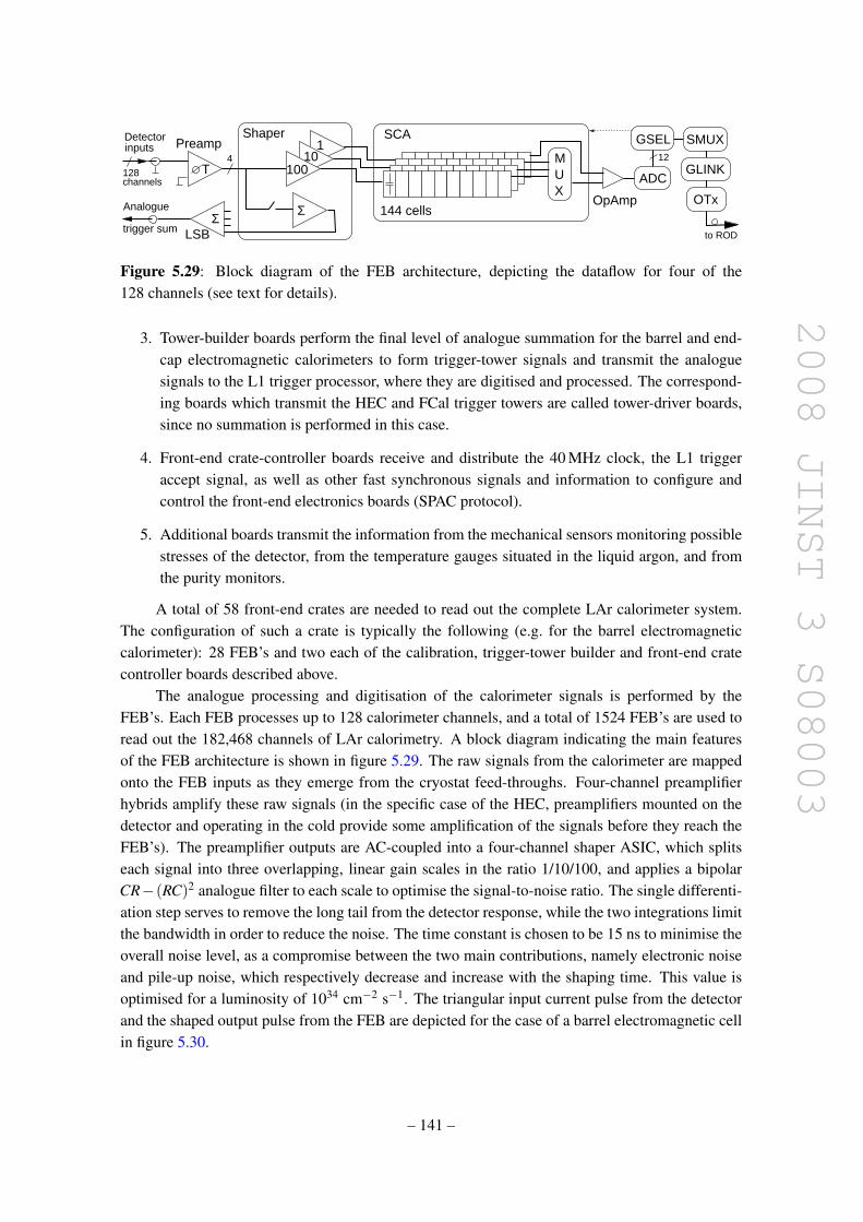
2008 JINST 3 S08003

Σ

101

100

Σ

ShaperPreamp

LSB

TADC

SMUX

OTx

MUX

144 cells

4

SCA

128

Analogue

trigger sum

channels

Detectorinputs

OpAmp

to ROD

12GLINK

GSEL

Figure 5.29: Block diagram of the FEB architecture, depicting the dataflow for four of the128 channels (see text for details).

3. Tower-builder boards perform the final level of analogue summation for the barrel and end-cap electromagnetic calorimeters to form trigger-tower signals and transmit the analoguesignals to the L1 trigger processor, where they are digitised and processed. The correspond-ing boards which transmit the HEC and FCal trigger towers are called tower-driver boards,since no summation is performed in this case.

4. Front-end crate-controller boards receive and distribute the 40 MHz clock, the L1 triggeraccept signal, as well as other fast synchronous signals and information to configure andcontrol the front-end electronics boards (SPAC protocol).

5. Additional boards transmit the information from the mechanical sensors monitoring possiblestresses of the detector, from the temperature gauges situated in the liquid argon, and fromthe purity monitors.

A total of 58 front-end crates are needed to read out the complete LAr calorimeter system.The configuration of such a crate is typically the following (e.g. for the barrel electromagneticcalorimeter): 28 FEB’s and two each of the calibration, trigger-tower builder and front-end cratecontroller boards described above.

The analogue processing and digitisation of the calorimeter signals is performed by theFEB’s. Each FEB processes up to 128 calorimeter channels, and a total of 1524 FEB’s are used toread out the 182,468 channels of LAr calorimetry. A block diagram indicating the main featuresof the FEB architecture is shown in figure 5.29. The raw signals from the calorimeter are mappedonto the FEB inputs as they emerge from the cryostat feed-throughs. Four-channel preamplifierhybrids amplify these raw signals (in the specific case of the HEC, preamplifiers mounted on thedetector and operating in the cold provide some amplification of the signals before they reach theFEB’s). The preamplifier outputs are AC-coupled into a four-channel shaper ASIC, which splitseach signal into three overlapping, linear gain scales in the ratio 1/10/100, and applies a bipolarCR−(RC)2 analogue filter to each scale to optimise the signal-to-noise ratio. The single differenti-ation step serves to remove the long tail from the detector response, while the two integrations limitthe bandwidth in order to reduce the noise. The time constant is chosen to be 15 ns to minimise theoverall noise level, as a compromise between the two main contributions, namely electronic noiseand pile-up noise, which respectively decrease and increase with the shaping time. This value isoptimised for a luminosity of 1034 cm−2 s−1. The triangular input current pulse from the detectorand the shaped output pulse from the FEB are depicted for the case of a barrel electromagnetic cellin figure 5.30.

– 141 –

2008 JINST 3 S08003

Figure 5.30: Amplitude versus time for triangu-lar pulse of the current in a LAr barrel electro-magnetic cell and of the FEB output signal afterbi-polar shaping. Also indicated are the samplingpoints every 25 ns.

The shaped signals are then sampledat the LHC bunch-crossing frequency of40 MHz by four-channel switched-capacitor ar-ray (SCA) analogue pipeline ASIC’s. The SCAstores the analogue signals during the L1 trig-ger latency in pipelines of 144 cells, and alsoserves as a multiplexer and de-randomisingbuffer in front of the ADC for triggered events.

For events accepted by the L1 trigger,typically five samples per channel and onlyone of the three gain scales are read out fromthe SCA. A gain-selector chip (GSEL) is usedto select the optimal readout gain individuallyfor each calorimeter channel and separately foreach L1 trigger. Two commercial dual op-ampchips couple the SCA outputs to commercial12-bit ADC’s used for the digitisation of theanalogue signals. The signals are formatted bythe GSEL, multiplexed (SMUX), serialised at 1.6 Gbits/s (GLINK), and then transmitted via asingle optical transmitter (OTx) based on vertical-cavity surface-emitting laser diodes (VCSEL).

Each shaper ASIC contains an analogue summing circuit, which sums its four channels as thefirst step in producing sums for the L1 trigger system. Channels can be individually enabled or dis-abled during FEB configuration in order to mask noisy channels. The four-channel sums are routedon the FEB to plug-in boards, which contain the next stage of the trigger analogue summing tree andwhich drive their output sums through the crate back-plane to the tower-builder (or tower-driver)boards, where the sums are completed before transmission off-detector to the L1 trigger system.

5.6.1.3 Tile calorimeter front-end electronics

The front-end electronics of the tile calorimeter are housed inside drawers located within thesteel girders which constitute the external support frame of the tile-calorimeter modules (see sec-tion 5.3.1.1). A block diagram of the tile-calorimeter front-end electronics and readout componentsinside the drawer is shown in figure 5.31.

A key element in the readout is the photomultiplier (PMT) block [131]. It is a mechanicalstructure comprising a steel cylinder and mu-metal shield for magnetic shielding, which containsa light mixer, a photomultiplier tube, a voltage divider and the so-called 3-in-1 card. The lightmixer is an optical plastic insert which mixes the light from the readout fibres to ensure uniformillumination of the photo-cathode. The PMT’s with their compact 8-dynode structure are used tomeasure the scintillation light [132]. All PMT’s were burned in and tested for linearity, stability,dark current and operating voltage for a nominal gain of 105 [112]. The average operating voltagefor nominal gain is 680 V. The assembled PMT blocks are inserted inside precision slots inside thealuminium structure of the drawers, which ensure accurate placement of the light mixer relative tothe fibre bundle for each readout cell.

– 142 –

2008 JINST 3 S08003

Fibres

Light mixer

Photomultiplier

Divider

Tiles

Calorimeter

3−in−1 Card

Laser

Particle energy

PMT block

Adder

ROD

Pipeline

ADC

Digitiser

Interface

Charge or energy

system

Mezzanine

Mother−board

TTC

Integrator

Current calibration

Bulk HVPSCesium

Probes

CANbus

Charge injection

MuonL1 trigger

CANbus

HVmicro−processor

Bulk LVPS

FingerLVPS

opto−couplerHV

CalorimeterL1 trigger

Figure 5.31: Block diagram of tile-calorimeter readout electronics.

The high voltage for each PMT is regulated with an accuracy of better than 0.25 V by micro-controllers inside the drawer. A single micro-controller services up to 48 PMT channels and hasa memory into which the nominal and set values of the voltage for each PMT are loaded. Eachhigh-voltage distributor system drives seven temperature probes located at key locations insideeach drawer.

Most analogue functions of the front-end electronics are contained on the 3-in-1 card [133].This board provides unipolar signal shaping to yield a pulsewidth of 50 ns and two linear outputswith a relative gain of 64 to achieve the overall 16-bit dynamic range required. The full scaleon the low-gain channel corresponds to 800 pC (the PMT gain is adjusted to provide approxi-mately 1 pC/GeV). Charge-averaging amplifiers on the 3-in-1 card are used for cell calibrationand monitoring and a charge-injection system is incorporated to calibrate the readout over its fulldynamic range. The 3-in-1 card also produces the analogue signals for the L1 trigger.

The digitiser system [134] samples the incoming data from the 3-in-1 cards every 25 ns usingtwo dedicated 10 bit ADCs (one for each of the low-gain and high-gain channels) and stores theinformation in a fixed-length pipeline, while waiting for a L1 trigger accept (L1A). Each digitiserservices up to six PMT channels. Each triggered event is recorded over an extended time frame,with a programmable length of up to 16 samples. In normal data-taking mode, following a L1A sig-nal, seven samples are kept: one close to the peak, four before the peak (with the two first samplesproviding a measurement of the signal pedestal) and two after the peak.

– 143 –

2008 JINST 3 S08003

There is one interface board [135] per pair of drawers. It receives and distributes the timing,trigger and control (TTC) signals, collects and formats data from the digitiser cards, and transmitsthe digitised data via an optical link. The interface board also performs cyclic redundancy checkson the input and output datastreams.

A system of four linked mother-boards form the base of the readout system. They distributepower to the 3-in-1 cards, the ADC integrator, the mezzanine card and the adders. Each mother-board also contains circuitry which generates a precise reference voltage used by the 3-in-1 cardsfor charge injection and integrator calibration. The mezzanine card is mounted on the first mother-board in the drawer. It decodes control commands sent via the TTC system and sends them ondifferential serial lines to the 3-in-1 cards. These commands control the charge injection, integratorgain setting and calibration, trigger-output gating and integrator bus access for each 3-in-1 card.The mezzanine card can also receive commands via the ADC integrator card, which is mountedon the first mother-board. It sends and receives messages via a dedicated CANbus daisy chain.The micro-processor in the ADC integrator card queues commands to the mezzanine card. Itsets the integrator gain on a 3-in-1 card, multiplexes the 3-in-1 card onto the integrator readoutbus and reads out the charge induced by the cesium source, by minimum-bias events, or by theon-board calibration DAC. The ADC integrator can also read back 3-in-1 card status and controlinformation.

Adder boards [136] are distributed along the drawer mounted on the mother-boards. Eachadder board receives the analogue trigger outputs from up to six 3-in-1 cards. The inputs areconnected to form trigger towers. The adders perform an analogue sum of the input signals andsend two output signals via long cables to the L1 trigger system. One of these signals (towersignal) comprises the sum of all samples, the second one (muon output) contains only the last tile-calorimeter sampling. In the case of the gap and crack scintillators (see section 5.5), the adder boardprovides amplification to match the small signals from these scintillators to the signal amplitudesrequired by the L1 trigger boards. It also provides the sum of the signal in all four of the gap andcrack scintillators. The muon output from these adder boards (see figure 5.31) provides the signalfrom the scintillator covering the region 1.2 < |η | < 1.4. As mentioned in section 5.5, sixteenof these channels will be used for the trigger from the minimum-bias trigger scintillators duringinitial data-taking.

5.6.1.4 Back-end electronics

Overview of architecture. The back-end system [126, 137] for all calorimeters is housed in themain services cavern (USA15), located 70 m away from the detector, and contains three differentsub-systems: the readout driver (ROD) system, which constitutes the core of the back-end, thetrigger, timing and control (TTC) system, and the L1 trigger receiver. The back-end system readsthe data from the front-end electronics, and digitally processes the data before transmitting it tothe data acquisition system at a L1 trigger rate of up to 75 kHz for the physics data-taking modeand at a 10 kHz rate for the calibration mode. The back-end system also receives the TTC signals,distributes the timing clock and trigger to the front-end electronics and the ROD’s, and configuresand controls the front-end crates. All of these tasks must be performed fast enough to cope withthe above trigger rates.

– 144 –

2008 JINST 3 S08003

The ROD’s are responsible for receiving, digitally processing and formatting the data fromthe front-end electronics and for performing various data-integrity checks and higher-level moni-toring tasks. The ROD module comprises a ROD mother-board on which are plugged up to fourprocessing-unit mezzanine cards. Each processing unit houses two commercial Digital Signal Pro-cessor (DSP) chips operating at 720 MHz. Each DSP is preceded by an input buffer used to performdata-integrity checks as well as to reformat the input data to suit the DSP architecture. Followingeach DSP is an output buffer used to buffer processed events before transfer to the data acquisitionsystem. For each trigger, data from the TTC stream and from the front-end electronics are pushedinto the ROD modules, where they are checked, processed, formatted and sent on a readout link tothe ATLAS data acquisition system.

Optimal filtering. The most important task of the DSP is to apply an optimal-filtering methodto the signals, including the relevant calibration constants, in order to provide the deposited en-ergy (in GeV) and the signal timing (in ns) for each cell [138]. This optimal-filtering method is atthe core of the back-end processing role and has been implemented in all the calorimeter ROD’s.It calculates the energy E, the timing τ and a simplified χ2 for the shaped and digitised signal fromeach cell, by means of a weighted sum over the relevant sample amplitudes, si, expressed as:

E =n

∑i=1

ai(si− ped) Eτ =n

∑i=1

bi(si− ped) χ2 =

n

∑i=1

(si− ped−E(gi− τg′i)

)2, (5.1)

where n is the number of samples and ped is the pedestal value of the corresponding readoutchannel, and gi and g′i are respectively the normalised ionisation pulse shape and its derivative withtime. The optimal filtering weights, ai and bi, are evaluated while minimising the dispersion in Eand Eτ arising from electronics and pile-up noise, taking into account the noise auto-correlationmatrix and the pulse shape at the input of the digitiser.

Trigger, timing and control. Four VME crates are used to implement the timing trigger and con-trol (TTC) system, where up to two partitions are implemented in a single crate. Each TTC partitioncontains a controller and a local trigger processor (see section 8.2.3 and figure 8.12).

The trigger latency, which is the delay between the bunch-crossing time and the time whenthe L1 accept signal (L1A) arrives to the front-end electronics, has been minimised to a valuebelow 2.5 µs. The TTC rack location has been chosen to minimise the length of the TTC fi-bres to the front-end crates and the associated contribution to the trigger latency. In addition, theprogrammable delay lines of the calibration boards are preset to reproduce the timing of signalsgenerated by particles originating from the interaction point.

Receiver system. The receiver system is part of the trigger-sum chain and interfaces the tower-builder and tower-driver boards to the calorimeter L1 processor. One important function of thetrigger-sum chain is to convert the signal from energy to transverse energy. The final gain ad-justment is left to the receiver. Each receiver crate contains 16 receiver modules, two monitoringmodules and one controller module. The LAr system consists of six receiver crates: two for thebarrel electromagnetic, two for the EMEC’s and two for the HEC and FCal. Two additional cratesare for the tile calorimeters.

– 145 –

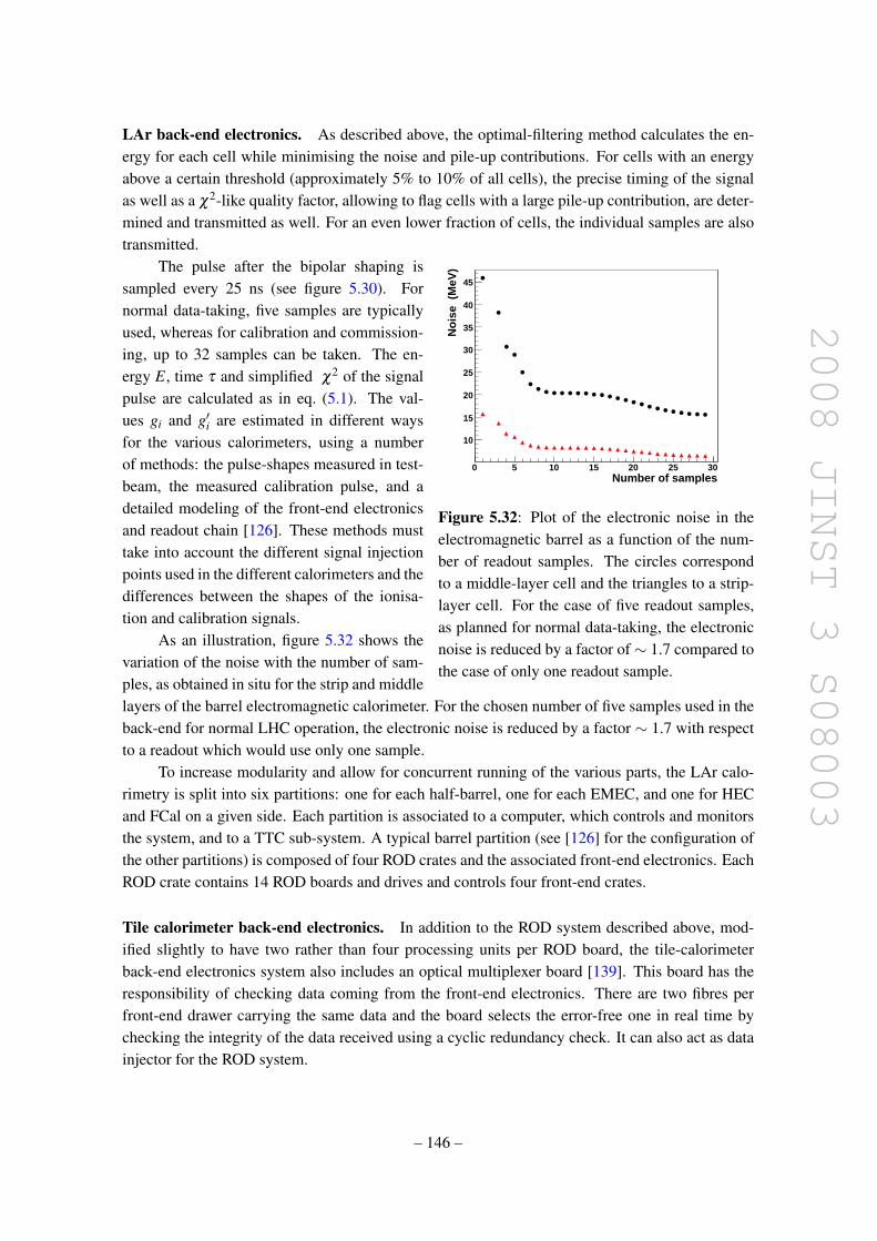
2008 JINST 3 S08003

LAr back-end electronics. As described above, the optimal-filtering method calculates the en-ergy for each cell while minimising the noise and pile-up contributions. For cells with an energyabove a certain threshold (approximately 5% to 10% of all cells), the precise timing of the signalas well as a χ2-like quality factor, allowing to flag cells with a large pile-up contribution, are deter-mined and transmitted as well. For an even lower fraction of cells, the individual samples are alsotransmitted.

Number of samples0 5 10 15 20 25 30

No

ise

(M

eV)

10

15

20

25

30

35

40

45

Figure 5.32: Plot of the electronic noise in theelectromagnetic barrel as a function of the num-ber of readout samples. The circles correspondto a middle-layer cell and the triangles to a strip-layer cell. For the case of five readout samples,as planned for normal data-taking, the electronicnoise is reduced by a factor of ∼ 1.7 compared tothe case of only one readout sample.

The pulse after the bipolar shaping issampled every 25 ns (see figure 5.30). Fornormal data-taking, five samples are typicallyused, whereas for calibration and commission-ing, up to 32 samples can be taken. The en-ergy E, time τ and simplified χ2 of the signalpulse are calculated as in eq. (5.1). The val-ues gi and g′i are estimated in different waysfor the various calorimeters, using a numberof methods: the pulse-shapes measured in test-beam, the measured calibration pulse, and adetailed modeling of the front-end electronicsand readout chain [126]. These methods musttake into account the different signal injectionpoints used in the different calorimeters and thedifferences between the shapes of the ionisa-tion and calibration signals.

As an illustration, figure 5.32 shows thevariation of the noise with the number of sam-ples, as obtained in situ for the strip and middlelayers of the barrel electromagnetic calorimeter. For the chosen number of five samples used in theback-end for normal LHC operation, the electronic noise is reduced by a factor ∼ 1.7 with respectto a readout which would use only one sample.

To increase modularity and allow for concurrent running of the various parts, the LAr calo-rimetry is split into six partitions: one for each half-barrel, one for each EMEC, and one for HECand FCal on a given side. Each partition is associated to a computer, which controls and monitorsthe system, and to a TTC sub-system. A typical barrel partition (see [126] for the configuration ofthe other partitions) is composed of four ROD crates and the associated front-end electronics. EachROD crate contains 14 ROD boards and drives and controls four front-end crates.

Tile calorimeter back-end electronics. In addition to the ROD system described above, mod-ified slightly to have two rather than four processing units per ROD board, the tile-calorimeterback-end electronics system also includes an optical multiplexer board [139]. This board has theresponsibility of checking data coming from the front-end electronics. There are two fibres perfront-end drawer carrying the same data and the board selects the error-free one in real time bychecking the integrity of the data received using a cyclic redundancy check. It can also act as datainjector for the ROD system.

– 146 –

2008 JINST 3 S08003

The ROD system of the tile calorimeter is physically divided into four independent partitions,two for the readout of the barrel calorimeter and one for each extended barrel calorimeter. Eachpartition is composed of a 6U VME TTC crate and a 9U VME ROD crate (containing eight RODprocessing-unit boards), which read out up to 64 front-end drawers. The ROD processing unitperforms various data-integrity checks and reconstructs the amplitudes of the digitised signals usingthe optimal-filtering method described above. Several algorithms based on optimal filtering arebeing developed to deal with detector and pile-up noise. The optimal-filtering method is also usedto reconstruct the signal in charge-injection calibration runs.

5.6.2 Calorimeter calibration systems

The LAr and tile calorimeters have very precise charge-injection systems and calibration boardsto calibrate the response of the front-end electronics boards. The tile calorimeter is equipped withtwo additional calibration systems to monitor the behaviour with time of the photomultipliers andof the optical components.

5.6.2.1 Calibration of LAr calorimeters

The aim of the electronic calibration is to determine the conversion factor, expressed as the ratiobetween the measured signal in ADC counts to the signal current in µA, for each individual channeland to monitor this factor with time.

The use of fast shaping for the calorimeter readout requires that the distribution of the cali-bration signals be done via injection resistors directly placed at the input of the detector cell andnot at the input of the preamplifier located outside the cryostat. This is shown in figure 5.33 forthe barrel and end-cap electromagnetic calorimeters for which the greatest precision is required. Inthe case of the HEC, the calibration pulse is injected in front of the cold preamplifiers. In the caseof the FCal, however, the calibration pulses are applied at the base-plane of the front-end crates,where the signals are split into two. One of the split pulses goes directly into the front-end boardsand the other goes through the cold electronics chain, reflects off the electrodes and is observed asa delayed pulse. The direct pulses are used to calibrate the electronics in the front-end crates andthe delayed pulses are used to examine problems related to the FCal and its cold electronics.

The conversion of the signal in µA to a signal in GeV has been obtained for all LAr calorime-ters from test-beam measurements. Figure 5.34 shows these conversions factors for the electro-magnetic calorimeters. This factor only changes once in the barrel when the absorber thicknesschanges at |η | = 0.8, whereas it changes almost continuously in the end-cap calorimeter becauseof the geometry and of the varying high-voltage. For the presampler cell energy scale, an effectivesampling fraction has been applied with a value of 1/20 for the barrel and of 1/60 for the EMEC.These values correspond approximately to the weights which have to be applied to the presamplersignal to correct for the energy loss of electrons before reaching the calorimeter. The conversionfactors in figure 5.34 agree with predictions based on Geant 4 simulations and knowledge of theLAr ionisation energy and drift velocity [140].

In the HEC1 wheel, this conversion factor is 0.306 µA/GeV and it is half that value for HEC2with its twice thicker absorber plates. The corresponding conversion factors for the FCal are 1.49,0.69 and 0.64 µA/GeV, respectively for FCal1, FCal2 and FCal3.

– 147 –

2008 JINST 3 S08003

DAC

6V

+2V

-

+

CKQ1 Q2

Rinj

Cd

C f

Ip

V(t)

ZcL R0

LAr

Ra

Rinj

Mother-board

Figure 5.33: Schematic diagram of the calibration system for the LAr electromagnetic calorime-ters. The components in the left part of the diagram are located on the calibration board itself atambient temperature in the front-end crates, whereas the right part of the diagram depicts the dis-tribution of the calibration signal into the calorimeter cells. This is achieved through the precisionresistors (Rinj), which are located on printed-circuit boards in the liquid argon. The impedanceof the cable between the calibration board and the printed-circuit boards in the liquid argon isdenoted Zc.

|η|0 0.5 1 1.5 2 2.5 3

A/G

eVµ

1.6

1.8

2

2.2

2.4

2.6

2.8

3

3.2

3.4EM Barrel

EM End-cap

Figure 5.34: Initial ionisation current per de-posited energy from electromagnetic showers inthe barrel and end-cap electromagnetic calorime-ters. These values have been derived from elec-tron test-beam data.

The calibration boards [129] are built todeliver a uniform, stable, linear and precisevoltage-driven signal with an amplitude andshape as close as possible to the calorimeterionisation current signal over a 16-bit dynamicrange (with currents up to 100 mA over 50 Ω).The triangular ionisation pulse is in practice ap-proximated by an exponential shape. The cho-sen distribution scheme, typically one calibra-tion channel every four signal channels, alsoallows the measurement of cross-talk [140].The largest cross-talk is between neighbouringstrips in the first layer of the electromagneticcalorimeter. It amounts to 5− 8% and is cor-rected for in the strip energy measurement. Thecalibration boards are equipped with programmable delays which are used to compensate the tim-ing differences due to the cable lengths. Apart from pedestal and gain measurements, a mea-

– 148 –

2008 JINST 3 S08003

surement of the pulse shape is performed by precisely delaying the trigger, using the TTCrx chiplocated on the calibration board. A total of 132 calibration boards have been produced. They fulfillthe required performance of an integral linearity better than 0.1%, a uniformity better than 0.2%,and a stability as a function of time better than 0.1%.

In the computation of the calibration constants for the electromagnetic calorimeter, however,a small difference in the response between physics and calibration pulses for the same initial cur-rent should also be taken into account. This arises from the different injection points of the current(see figure 5.33) and from the difference between the exponential current as a function of timefor the calibration and the triangular pulse shape of the physics pulse (see figure 5.30). This dif-ference depends on the electrical properties of the readout cells and on pseudorapidity and neverexceeds 4%. The procedure to compute this correction has been validated during the study of theresponse uniformity with test-beam data of production modules. For this reason, several calibrationmethods have been used to determine the optimal-filtering coefficients (see section 5.6.1.4).

5.6.2.2 Calibration of tile calorimeter

Each tile-calorimeter cell can be divided into three sections for calibration purposes; the opticalpart consisting of scintillator and fibres, the photomultipliers, and the front-end electronics whichshape and digitise the light signals. A calibration and monitoring system is used to certify each ofthese parts independently [141].

The charge-injection system is designed to calibrate the front-end shaping and digitising cir-cuits to an accuracy of 1%. It uses a precision DAC on each of the 3-in-1 cards, in conjunction withsolid-state switches and precision capacitors. Dedicated charge-injection runs are taken scanningthe full range of both gains. Fits to the measured pulses convert ADC counts to pC and yield a typ-ical non-linearity of about two ADC counts over the full dynamic range, with a stability of betterthan 1% over many months of monitoring.

The laser system is used to calibrate and monitor the photomultiplier response with a targetaccuracy of better than ±1%. This system sees both the front-end electronics and the photomul-tipliers. A Nd:YVO4 laser, synchronised to the TTC clock generates pulses of ∼ 10 ns length ata wavelength of 532 nm. The laser light is split in the main services cavern (USA15) and sentvia clear plastic fibres to each calorimeter finger where it is again split to each photocathode. Thepulse-to-pulse variation is monitored at the laser by several pin-diodes and, by means of a fil-ter wheel, the laser light intensity can span a dynamic range of 104. The global photomultipliernon-linearity is found to be < 0.5% above 80 pC and up to where saturation sets in. In addition,the system can be used to set the global calorimeter timing and to investigate saturation-recoverytechniques.

To calibrate and monitor the tile-calorimeter scintillator and optical system, a 137Cs γ-sourceof ∼ 10 mCi strength is moved hydraulically inside the calorimeter body. This system sees thefull chain from the optical part to the front-end electronics and to the photomultiplier. It enablesthe setting of the high voltage of each channel and inter-calibration of all the 10000 tile channels.These calibrations are performed during dedicated runs, with the source traversing each of the463,000 tiles in the detector [142]. The photomultiplier current is integrated by the 3-in-1 cards asthe source passes within the corresponding cell. From the digitised current, the response of each

– 149 –

2008 JINST 3 S08003

scintillator tile can be extracted. The accuracy of a single tile response is better than ±2%, andthe mean response accuracy for a calorimeter cell is ±0.3%. Based on monitoring a single moduleover a period of four months, the long-term stability of the system was determined to be 1%. Aprocedure to set the gains of each photomultiplier based on the integrated cell-source current allowsinter-calibration of cells and modules to better than ±3% [141]. The absolute energy calibration(pC/GeV) is set with electrons, as described in section 5.7.4.1.

5.6.3 Calorimeter power supplies and services

This section describes briefly the LAr and tile calorimeter power supplies, cooling systems andcontrols.

5.6.3.1 Low-voltage power supplies

The low-voltage power supplies for the LAr and tile calorimeters are located in the main cavern, asclose as feasible to the on-detector electronics boards. To this end, they had to be custom built andvalidated to operate in a high radiation environment, in a significant residual magnetic field of upto 100 mT, and in a very limited volume.

Each front-end crate of the LAr calorimeter is powered by a low-voltage power supply locatedclose to it in the gap between the cryostats. This power supply delivers with multiple, redundantDC-DC converters, the seven DC voltages necessary to the front-end crate. There are a total of 58low-voltage power supplies, 2× 16 for the barrel electromagnetic calorimeter and 2× 13 for theend-cap calorimeters. Each low-voltage power supply is powered by a 280 V DC power supplylocated in the underground counting room (USA15). The low-voltage power supplies and associ-ated 280 V power supplies are controlled and monitored using a custom interface board, ELMB,described in section 8.5.

Low-voltage power to the tile-calorimeter drawer electronics is supplied by a custom powersupply located in a mechanical extension on the ends of the module. These extensions are locatedon either side of the central barrel and on the outer surface of each extended barrel at the supportgirder. Each water-cooled power supply consists of eight isolated switching DC-to-DC convertors(bricks) which are powered by a customised external 200 V DC bulk power supply. The bricksthemselves are controlled and monitored at two levels externally through CANbus using a custominterface board based on the ELMB described in section 8.5 and using current loops. An indepen-dent external reset from USA15 is available in the case of a failure in the voltage control network(for example due to a single event upset). A second auxiliary board, also based on the ELMB andlocated in USA15, provides overall control.

5.6.3.2 High-voltage power supplies

High voltage is delivered to the LAr and tile calorimeters through commercial or custom-builtexternal power supplies located in the underground counting room.

Several different versions of the same industrial power supply are used to power the differentLAr detectors, according to the voltage and current needed. The maximum voltage and currentof each version are given in table 5.6. Furthermore, the barrel electromagnetic, EMEC or HEC

– 150 –

2008 JINST 3 S08003

Table 5.6: Nominal voltages, maximum voltage and maximum current of the differentLAr calorimeter high-voltage power supplies.

Nominal Maximum MaximumDetector detector voltage module voltage module current

(V) (V) (µA)Electromagnetic barrel 2000 2500 75

Barrel presampler 2000 2500 75Electromagnetic end-cap (EMEC) 1000 to 1700 2000 200

1800 to 2500 2500 200End-cap presampler -2000 -2500 75

Hadronic end-cap (HEC) 1800 2500 75Forward calorimeter (FCal) 250, 375, 500 600 6000

Purity monitors ±2500 ±2500 75

channels showing a problem, such as a resistive short, are powered by high-current (maximumof 3 mA) supplies. A power supply module contains two boards with 8 (FCal) or 16 (all detectorsbut FCal) channels each. All high-voltage channel parameters can be controlled remotely and inparticular the voltage itself, the ramp speed and the trip levels for the current drawn. In total, thereare 157 modules housed in 20 crates containing eight modules each for the whole LAr system.

High voltage is delivered to the tile-calorimeter drawers from external bulk power supplies.The supply can deliver two voltages to the input of the drawer (-830 V and -950 V) to match thePMT operating requirements and provides a maximum current of 20 mA. The voltage is distributedinside the drawer and regulated to provide the desired voltage for each PMT. A single bulk supplyprovides high voltage to 16 drawers.

5.6.3.3 Cryogenics and cooling

The cryogenics services for the LAr calorimeters are described in some detail in section 9.4.5 andshown in figure 9.6. The cooling systems for the LAr and tile calorimeter electronics are bothbased on a leak-less system for the on-detector implementation (see section 9.4.3 for an overviewof the off-detector systems). The cooling system supplies demineralised water at 18C and workswith sub-atmospheric pressure to prevent the cooling liquid from leaking out of the system shoulda break or holes occur in a cooling pipe.

The total consumption of the LAr front-end readout electronics exceeds 200 kW (each FEBchannel has a consumption of ∼ 0.7 W). Therefore, each electronic board in a front-end crateis conductively cooled using two aluminium plates placed on each side of the board. These alu-minium plates are implemented as part of the leak-less cooling system. The temperature of a FEBis maintained constant at±1C. Under these conditions, no temperature dependence is observed onthe pedestals, the gains and the delays of the readout electronics. The low-voltage power suppliesare also operated using the same cooling system.

A heat dissipation of 300 W is expected from a pair of tile-calorimeter drawers and a leak-less cooling system [143] provides cooling inside the drawers. The performance requirementswere determined with a prototype system [144] which was used during the calibration of produc-tion modules in a test-beam. By varying the input temperature and flow-rate it was possible to

– 151 –

2008 JINST 3 S08003

change the temperature inside the drawer while measuring the response of the calorimeter to ahigh-energy pion beam. The fractional energy variation as a function of temperature changes ofthe PMT block was found to be 0.2%/C and the variation in response of the PMT gain itself as afunction of temperature changes of the cooling water is 0.15%/C. To ensure a PMT gain stabilityof ±0.5%, the temperature variations of the PMT block must be smaller than ±2.5C. Long-termtests carried out during calibration of production modules showed that the system could maintainthe temperature in a drawer to within ±0.3C.

5.6.3.4 Detector control systems

Within the context of the overall ATLAS detector safety (DSS) and control (DCS) systems de-scribed in section 8.5, this section describes the main operating parameters monitored by the spe-cific DCS implementations of the different calorimeter systems.

LAr controls. The LAr DCS controls and monitors two important operational parameters: theliquid-argon temperature and purity.

• Temperature measurements

The measured sensitivity [140] of the LAr signal to temperature is −2% per degree. Numer-ous calibrated (∆T = 10 mK) temperature probes (PT100 platinum resistors) have thereforebeen installed in each calorimeter to measure precisely the liquid-argon temperature. A totalof 192 temperature probes are glued on the absorbers of the barrel electromagnetic calorime-ter at two radii (inner and outer) and regularly distributed in z× φ (6× 32). Similarly, atotal of 32 (respectively 18) temperature probes are located at the front and back sides of theexternal (respectively internal) EMEC wheels, close to their outer radius. These probes arealso uniformly distributed in φ .

A total of 192 HEC temperature probes fixed on copper blocks at three radii (inner, mid-dle and outer) are located near the HEC-wheel rear surface and uniformly distributed in φ .Finally, the three FCal modules are equipped with a total of 14 temperature probes, four atthe outer radius and ten at the inner radius, where heating from beam interactions and heattransfer through the cryostat wall is highest. These sets of temperature probes are completedby other sets, used to control and monitor the temperature during the cooling or heating ofthe cryostats.

• Purity monitors

To control the argon purity, ten purity monitors have been installed on the outer radius of thebarrel calorimeter between the support rings. They are located in the median azimuthal planeand at the top and the bottom of the half-barrels. Ten purity monitors are also installed in eachend-cap cryostat, two in the EMEC region, six in the HEC region and two in the FCal region.The impurity measurement is based on the energy deposition by radioactive sources in theliquid argon. The ionisation charge is collected by an electric field and measured by a coldpre-amplifier. Each device consists of two radioactive sources: an 241Am source, whichemits 5.5 MeV α-particles, and a 207Bi source, which emits 1 MeV conversion electrons.

– 152 –

2008 JINST 3 S08003

The ratio of the measured charges between the Bi and Am sources is used to extract theabsolute oxygen content in the liquid argon [107]. The oxygen contamination in the barrelLAr cryostat has been monitored to remain below 0.3 ppm since more than a year of coldoperation in the ATLAS pit and is stable to better than a few %. The argon purity achievedis thus well within specification.

The other quantities controlled and monitored by the LAr DCS are mainly concerned with thereadout electronics. On the detectors, DCS controls also the voltage, the current and the tempera-ture of the HEC front-end power supplies. On the high-voltage system, DCS controls the voltage,the intensity and the pre-set value for switching off each high-voltage channel. The temperature ofeach high-voltage module is also monitored. On the front-end electronics, DCS controls the powersupplies and monitors the voltage, the current and the status of the 280 V power supplies, whichpowers the front-end crates, and of the low-voltage power supplies in the front-end crates (thetemperature of each FEB is monitored by the DAQ system). Finally, on the back-end electronics,DCS monitors the voltage, the current and the temperature of each crate.

Tile controls. The tile-calorimeter DCS controls and monitors mainly the on-detector low-voltageand high-voltage power supplies and electronics cooling, as well as the off-detector high-voltageand bulk 200 V DC power supplies, auxiliary boards and electronics racks. The communicationwith the high-voltage bulk power-supply crates is done using RS422. CANbus is used for thecommunication with the micro-controller cards located on the high-voltage side of the drawers. Aclient-server system has been developed and commissioned for the control and monitoring of thephotomultiplier high voltages. Control and monitoring of the on-detector low-voltage power sup-plies is implemented via a custom auxiliary board, which multiplexes currents and temperaturesfrom sensors inside the drawers, and communicates via CANbus. The 200 V DC power suppliesare controlled and monitored using Modbus.

A total of more than 30,000 parameters are monitored in this system. Configuration data suchas system structure (lists and hierarchies of devices), device properties (configuration of archiving,smoothing, etc.) and settings (output values, alert limits) are stored in the configuration database.The data produced is stored in the DCS ORACLE-based archive. Due to the large amount of datamonitored by DCS, smoothing is applied to reduce the amount of data stored. A subset of thesedata (for example photomultiplier high-voltage settings) is also available to offline reconstruction.

5.7 Test-beam measurements and results

5.7.1 Electromagnetic module performance

Four (of 32) barrel and three (of 16) end-cap production modules have been exposed to test-beamswith a set-up which includes a cryostat on a moveable table, enabling detailed position scans. Thesetests have been carried out in the CERN SPS H8 and H6 beam lines, using electron and positronbeams of energies between 1 and 250 GeV. A comprehensive analysis of module performance hasbeen reported [140, 145, 146].

The electron energy reconstruction procedure is similar to that described in section 10.4: forexample, for the barrel electromagnetic calorimeter, an electron cluster is first constructed using

– 153 –

2008 JINST 3 S08003

the measurements in the middle accordion layer, where cells within a square window of 3×3 cellsaround the cell with the highest energy are clustered together. For the other accordion layers, allcells intersecting the geometrical projection of this square window are included. The energy ineach layer, E0 for the presampler and E1, E2, E3 for the strip, middle and back layers, is the sumof the energies of the selected cells in the cluster. The energy of the electron is then given by thealgorithm:

E = offset + w0×E0 + w01×√

E0E1 + λ (E1 +E2 +E3) + w3×E3,

where the offset and w0 correct for the energy lost upstream of and in the presampler, w01 cor-rects for the energy deposited in the dead material between the presampler and the strip layer,λ corrects for the energy dependence of the sampling fraction and for lateral leakage outside theelectron cluster, and w3 corrects for the energy deposited downstream of the calorimeter. Thesecoefficients depend somewhat on the electron energy and the η value. An iterative procedure istherefore needed to reconstruct the electron energy. This procedure has been shown to convergeafter two iterations. The correction coefficients have been determined by simulating the test-beamset-up using GEANT4. In the case of the EMEC, where the presampler is present only in the re-gion 1.5 < |η | < 1.8, where the material in front of the calorimeter was independent of η , andwhere the beam energy did not exceed 180 GeV, a similar but simplified scheme is used [140].

For the barrel electromagnetic calorimeter, the linearity of the response and the energy reso-lution have been studied as a function of energy in the range from 10 to 245 GeV at η = 0.687.At 245 GeV, the beam energy was not known well enough and the linearity of response could notbe assessed accurately. The experimental measurements, after noise subtraction, have been fittedwith the expression [146]:

σ(E)E

=a√

E(GeV)⊕b, (5.2)

where a is the stochastic term and b the constant term reflecting local non-uniformities in theresponse of the calorimeter. In the energy range 15−180 GeV, the reconstructed energy responseis linear within ±0.1%, as shown in figure 5.35. For the lowest-energy point at 10 GeV, a non-linearity of 0.8% is measured. A stochastic term of 10% ·

√GeV and a constant term of 0.17%

have been obtained from the fit to the fractional energy resolution, as illustrated in figure 5.36.These results are in agreement with dedicated Monte-Carlo simulations of the test-beam set-up.Similar results for the energy resolution have been obtained for the EMEC [110].

At low energy, the calorimeter response to minimum-ionising particles has provided a detailedexploration of the structure of the active material of the detector. In particular, the muon energydeposition is much more localised than the electron energy depositions. Typically, muons onlycross one middle cell in η and one or two in φ . They can therefore be used to study the finestructure of the calorimeter, without having to deconvolute the effects of the showering process.The signal-to-noise ratio, evaluated as the ratio of the most probable energy deposit divided by theRMS spread of the pedestal, varies between seven and twelve for middle barrel cells and betweensix and seven for middle end-cap cells. These results have shown that cosmic muons can be used tocommission the favourably oriented part of the electromagnetic calorimeters in terms of timing andresponse uniformity, and may serve to verify the integrity of the detector and of the whole readoutchain before the start-up of the LHC [147].

– 154 –

2008 JINST 3 S08003

(GeV)beamE0 20 40 60 80 100 120 140 160 180 200

bea

mE

/E

0.99

0.992

0.994

0.996

0.998

1

1.002

1.004

1.006

1.0‰±

DataBeam energy uncertainty

(GeV)beamE0 50 100 150 200 250

/E

Eσ

0.01

0.015

0.02

0.025

0.03

0.035

0.04 0.17 %⊕ E/E = 10.1 %/Eσ

Data

Figure 5.35: Linearity of response as afunction of the electron beam energy, Ebeam,for a barrel LAr electromagnetic moduleat |η | = 0.687. All points are normalised to thevalue measured at Ebeam = 100 GeV. The bandrepresents the total uncertainty on the beam en-ergy measurement.

Figure 5.36: Fractional energy resolution asa function of the electron beam energy, Ebeam,for a barrel LAr electromagnetic moduleat |η | = 0.687. Electronic noise was subtractedfrom the data before plotting the results. Thecurve represents the results of a fit to the datausing eq. 5.2.

The response uniformity at high energy as a function of η has been measured using an elec-tron beam of 245 GeV for the barrel and of 119 GeV for the end-cap [140]. The goal for AT-LAS is to achieve a constant term of 0.7% or smaller over the full calorimeter acceptance. Non-uniformities of the response on the tested modules do not exceed 0.7% and do not exceed even 0.5%in the case of the barrel modules, as shown in figure 5.37. The overall constant term in the energyresolution, using the above formula, ranges between 0.5% and 0.7% and therefore meets well thecalorimeter design performance goals.

The performance of the barrel electromagnetic calorimeter in terms of its finely segmentedfirst sampling has been studied by using electron, photon and pion beams [145]. The positionresolution along η was measured to be about 1.5×10−4 and 3.3×10−4 (in units of pseudorapidity)at 245 GeV for the front and middle layers, allowing to achieve a polar angle resolution in therange 50–60(mrad)/

√E (GeV) over the whole coverage (barrel and end-caps). The π0 rejection

was measured from real data, using a photon beam and mixing together different events to mimicphoton pairs from π0 decays, and found to be 3.54±0.12 (statistical) for π0 with pT = 50 GeV andfor a single photon efficiency of 90%.

A spare electromagnetic barrel module, identical to the series modules, was built for thecombined test-beam period described in section 10.1.2 and was exposed to electron, photon, pionand muon beams with energies between 1 and 350 GeV. The amount of material in front of thismodule was very close to the material expected in ATLAS and therefore great importance was givento the task of verifying that the linearity, energy resolution and uniformity [148] are well understoodin terms of the detector description and the simulations using GEANT 4. The performance ofthe electromagnetic calibration scheme, using longitudinal weights similar to the ones describedabove, was tested by adding in a controlled way different amounts of material just in front of theelectromagnetic calorimeter. This extra material corresponded to 2.4–3.3 X0 and emulated in thisway the material in front of the LAr barrel calorimeter in ATLAS in the region |η |< 1.2. A linearity

– 155 –

2008 JINST 3 S08003

0.96

0.98

1

1.02

1.04

0.5 1 1.5 20

0.05

0.1

0.15

0.2

0.25

0.3

0.35

0.4

η

Uni

form

ity

+2 %

+1 %

-1 %

-2 %All barrel: 0.43% All EMEC: 0.62%

882 cells 2455 cells

OV

ER

LA

P

Figure 5.37: Distribution of the average energies measured in all cells of all tested modules as afunction of the cell η , normalised to the mean energy measured in the modules. In the barrel, thismean energy was ∼ 245 GeV, while it was ∼ 120 GeV in the EMEC. For each bin in η , the distri-bution is normalised to the number of middle cells in that bin (design value). This normalisation isonly used to define the colour of each bin in the plot.

of 0.5%, independent of the upstream material, is obtained over the energy range 20–250 GeV,as shown in figure 5.38. Figure 5.39 shows the noise-subtracted (σnoise = 170 MeV) resolutionat η = 0.4 for an amount of upstream material of 2.4 X0. The data points have been corrected forthe beam momentum spread. A stochastic term of (10.1 ± 0.4)%×

√GeV and a constant term

of (0.2 ± 0.1)% are obtained and the data are well described by the simulation, which incorporatesthe most detailed and up-to-date description of the detector and GEANT 4 (version 4.8.2) model ofelectromagnetic showers. More detailed results from this last test-beam period for the barrel LArelectromagnetic calorimetry can be found in [149].

5.7.2 Hadronic end-cap performance

About 25% of the series production modules were exposed to beams of muons, electrons and pionswith energies up to 200 GeV at the CERN SPS [150]. Two partial HEC wheels, consisting of threeHEC1 and three HEC2 modules were used. The goal was not only to prove the uniformity of theproduction modules as defined by the hardware tolerances, but also to determine their performanceand calibration, as obtained from muons, electrons and pions. The data taken with electrons yielda fractional energy resolution after noise subtraction and a fit to the functional form in eq. (5.2)with a stochastic term, a = (21.4±0.1)% ·

√GeV and a constant term, b, compatible with zero, in

good agreement with predictions from simulation [150]. Horizontal and vertical scans with beamsacross the surface of the calorimeter showed a homogeneity of the electron signal of± 1% withoutcorrections.

The pion measurements are of particular importance for the prediction of the final perfor-mance of the calorimeter for jets. A stochastic term of (70.6± 1.5)% ·

√GeV and a constant

term of (5.8± 0.2)% were obtained from a fit to the functional form in eq. (5.2). The data have

– 156 –

2008 JINST 3 S08003

(GeV)beamE0 50 100 150 200 250

beam

E/E

0.98

0.99

1

1.01

1.020 0 mm = 2.4 X025 mm = 2.7 X050 mm = 3.0 X075 mm = 3.3 X

(GeV)beamE0 50 100 150 200 250

/EEσ

0

0.01

0.02

0.03

0.04

0.05 0.1)%± (0.4 ⊕ E 0.4)%/±/E = (10.0 EσData:

0.2%⊕ E 0.1)%/±/E = ( 9.6 EσSimulation:

Figure 5.38: Linearity of response as a func-tion of the beam energy, Ebeam, at |η | = 0.687,for a barrel LAr electromagnetic module inthe combined test-beam set-up exposed to elec-tron beams with different amounts of materialplaced upstream of the active calorimeter.

Figure 5.39: Fractional energy resolution asa function of the electron beam energy, Ebeam,for a barrel LAr electromagnetic module in thecombined test-beam. Electronic noise has beensubtracted from the data. The results are shownfor an amount of upstream material of 2.4 X0,which is that expected in ATLAS at η = 0.4.The curves represent the results of fits to thedata and the simulation using eq. 5.2.

been compared in detail to simulations (GFLUKA, GCALOR and GHEISHA) with satisfactoryresults [151].

From 2002 to 2004, a new set of combined test-beam measurements was launched. The mainpurposes were to define calibration procedures and constants for initial operation in ATLAS andto operate the EMEC, the HEC and the FCal together in conditions as close as feasible to thoseexpected in ATLAS. The first of these combined test-beam periods took place in 2002 and wasdevoted to the region 1.6 < |η | < 1.8 [152, 153]. The second period took place in 2004 and wasdedicated to a scan of the transition region around |η |= 3.2.

A three-dimensional clustering algorithm and a signal-weighting approach (see sec-tion 10.5.2), used already in previous experiments, have been tested and the first results yield goodenergy resolution for pions. The signal-weighting technique exploits the fact that local energydepositions of high density are mainly due to electromagnetic interactions, whereas for hadronicinteractions, the corresponding density is substantially lower. Thus, for a segmented calorimeter,the energy deposited in individual readout cells can, on a statistical basis, be identified to be ofelectromagnetic or hadronic origin. For ATLAS, these weights are derived from simulations ofsingle particles and jets. In test-beam, the volume of the related clusters in EMEC and HEC hasbeen used to obtain the cluster energy density. The weighting function has been derived from thedata directly, but after correcting for leakage (for details see [152]).

Figure 5.40 shows the energy dependence of the fractional energy resolution separately forthe π− and π+ data. For energies up to 80 GeV, a differential Cerenkov counter has been usedto separate π+ and protons. The proton contamination in the beam increases with energy and itscontribution to the π+ data in figure 5.40 is the dominant source of systematics when comparingthese data to the π− data and to simulation. Fits to the data using eq. (5.2) yield stochastic terms

– 157 –

2008 JINST 3 S08003

(GeV)recoE0 50 100 150 200

/ E

Eσ

-110

data-π

data+π

G4 (LHEP)

G4 (QGSP)

(mm)beam

y-200 -150 -100 -50 0 50 100 150 200

En

erg

y re

spo

nse

(G

eV)

0

20

40

60

80

100

120

140

160

180

200Total

FCal1

FCal2

EMEC

HEC

Figure 5.40: Fractional energy resolution as afunction of reconstructed energy for π− and π+

data taken during the 2002 EMEC/HEC com-bined test-beam period compared to differentpredictions from simulation using GEANT 4.The analysis employs the signal-weightingtechnique described in the text. The data areplotted after noise subtraction and the curverepresents as an example a fit to the π+ datausing eq. (5.2).

Figure 5.41: Energy response on the elec-tromagnetic scale for 200 GeV pions whenperforming a vertical scan across the transi-tion region between the EMEC/HEC and FCalcalorimeters. Shown is the total energy re-sponse together with the individual responsesin the different electromagnetic and hadroniccomponents of the calorimetry. The data (fullsymbols) are compared to GEANT 4 predic-tions (open symbols).

of (84.6± 0.3)%√

GeV and of (81.7± 0.4)%√

GeV for π− and π+ respectively, and constantterms of zero within errors. The energy range available is not extensive enough to avoid any cor-relation between the stochastic and constant terms. Nevertheless, the results give some indicationof the effectiveness of the signal-weighting technique in achieving a good level of compensation.The GEANT 4 simulations (version 5.0) with two different hadronic physics lists (LHEP 3.3 andQGSP 2.3) shown in figure 5.40 are in reasonable agreement with the data, but neither model yieldsan optimal description of the data [151].

The scan of the transition region around |η | = 3.2 was meant to assess the performance in thecomplex region of overlap of the three end-cap calorimeters. The EMEC, HEC and FCal moduleswere positioned as in ATLAS, including mock-ups of the details of cryostat walls and supports(dead material). One quarter of the full HEC1 and HEC2 wheels were assembled with dedicatedsmall modules having reduced η-coverage and encompassing only the forward region. Simi-larly, one EMEC inner-wheel module (one-eighth of the full EMEC wheel) and one quarter ofthe full FCal1 and FCal2 detectors were assembled. The results of this scan for the performanceof the EMEC, HEC and FCal on the electromagnetic scale are described in [154]. These resultsdemonstrate that the response and resolution of electrons and pions across most of the EMEC/HECand FCal acceptance, including the crack region around η = 3.2, show reasonable agreement withexpectations from detailed simulation.

As an example, figure 5.41 shows the response on the electromagnetic scale for 200 GeV pi-ons, when moving from the FCal region (left) across the crack to the EMEC/HEC region (right).Shown is the total energy response together with the individual responses in the different electro-

– 158 –

2008 JINST 3 S08003

magnetic (FCal1 and EMEC) and hadronic (FCal2 and HEC) components of the calorimeter. Forthe energy reconstruction, a cone size of ∆R×∆φ = 0.30 has been used. The data are comparedwith simulation (GEANT 4, version 7.1 with physics list QGSP-GN 2.6). The prediction for thetotal electromagnetic energy measured in the FCal region shows some deviations from the data. Asalready known from previous studies with the QGSP physics list, the simulation tends to predicttoo compact hadronic showers in comparison to the data. But the general loss of signal (on theelectromagnetic scale), when traversing the crack region is not more than ∼ 20%. The details ofthe complex material structure in the crack region are rather well described in the simulation.

5.7.3 FCal performance

There have been two FCal stand-alone test-beam periods at the CERN SPS, one in 1998 and onein 2003. The 1998 period used engineering modules which were full-depth segments of FCal1and FCal2. The electron response of FCal1 and an estimate of the electromagnetic scale for FCal2were extracted from these measurements [155]. The 2003 test-beam was carried out with thefinal production modules and used electronics which were very similar to the final electronics im-plemented for ATLAS. Data were taken with electron and pion beams with momenta from 10to 200 GeV. The data were analysed using the standard LAr technique of optimal filtering (see sec-tion 5.6.1.4). Electronic noise was calculated from the data and was subtracted in quadrature beforeenergy resolution plots, such as those shown in figures 5.42 and 5.43, were produced.

Figures 5.42 and 5.43 illustrate the results obtained after subtraction of the electronic noisefrom the data. The points have been fitted with the function in eq. (5.2). The fit to the electrondata in figure 5.42 yielded stochastic and constant terms of (28.5±1.0)%

√GeV and (3.5±0.1)%,

respectively. For pions, the energy resolution depends on the technique used to correct the re-constructed energies from the electromagnetic scale to the hadronic scale. Two techniques wereemployed: the first one uses a single weight per module (flat weights) and yields stochastic andconstant terms of (94.2±1.6)%

√GeV and (7.5±0.4)%, respectively. A more sophisticated tech-

nique, using radial weights, which exploits the fine transverse segmentation of the FCal, improvesthe sampling term from 94% to 70% and yields a constant term of 3.0%. The measured energyresolution for pions with an energy of 200 GeV is improved from 10.1% to 5.8% as shown in fig-ure 5.43.

The resolutions obtained in these FCal beam tests meet well the design specifications, whichwere expressed as stochastic and constant terms of 100% and 10% respectively for hadrons. Furtherdetails of the results of the 2003 test-beam measurements can be found in [156].

5.7.4 Tile-calorimeter performance

5.7.4.1 Stand-alone performance

Approximately 12% of all production modules of the tile calorimeter have been measured exten-sively in dedicated test-beam periods at the CERN SPS.

Muons with an energy of 180 GeV and incident at 90 to the module symmetry plane wereused to study the photo-electron yield for all eleven tile sizes in the detector (monitoring the photo-electron yield checks for any deterioration in time of the optical response of the calorimeter).

– 159 –

2008 JINST 3 S08003

(GeV)beamE

0 50 100 150 200

/ E

(%

)Eσ

0

2

4

6

8

10

12

14

(GeV)beamE

0 50 100 150 200

/ E

(%

)Eσ

0

10

20

30

40 Flat weights

Radial weights

Figure 5.42: Fractional energy resolution ob-tained for electrons measured in the first mod-ule of the forward calorimeter as a functionof the beam energy, Ebeam. The curve corre-sponds to the result of a fit to the data pointsusing eq. 5.2.

Figure 5.43: Fractional energy resolution ob-tained for pions, measured in all three modulesof the forward calorimeter, as a function of thebeam energy, Ebeam. The data are shown fortwo cell-weighting schemes and the curves cor-respond to the result of a fit to the data pointsusing eq. 5.2.

The photo-electron yield was calibrated using two independent techniques. The first one uses thespread in the difference of signals from the two photomultiplier tubes for muons passing throughthe centre of the cell. The second one uses the spread in the laser-generated light to calibratethe photomultiplier response in photo-electrons per pC and the measured signal for muons andelectrons. The results of the two methods are in excellent agreement: the light yield is independentof the size of the tiles within 1–2% uncertainties. These results also reproduced the batch-to-batch light output variation seen during tile production, together with the systematic differenceassociated with the two sources of raw polystyrene (the photo-electron yield is about 80 per GeVfor one source and about 100 per GeV for the other source). In the extended-barrel modules, theyield is 10% to 20% lower, reflecting the choice which was made to use batches with higher lightyields for the barrel modules. The muon data at 90 incidence also provided the means to studythe local and global features of the calorimeter response. The spread of the mean signals from theeleven tile sizes is 2.0% (respectively 2.8%) for the barrel (respectively extended-barrel) modulesand the spread within each tile size is about 3%. The average response of a module varies betweenmodules with a spread of 1.2%, while the variation within a given module is typically 4–5%.

The muon signal-to-noise ratios are very large, typically 44 when summing over a tower(three radial layers and over ∆η ×∆φ ≈ 0.1× 0.1) and 18 in the last radial layer. This feature isexpected to provide reliable identification of isolated muons down to energies of ∼ 2 GeV even inthe presence of pile-up noise, which is negligible in the last layer. The response to 180 GeV muons,averaging over angles in the range −1.49 < |η | < 1.35 has a spread of 1.9% (rms), excludingangles for which the coverage is not complete.

The modules were exposed to electron beams with energies between 10 and 180 GeV, toset the energy conversion scale (i.e. the photomultiplier high voltage to be supplied, as discussedin section 5.6.1.3) for a significant fraction of the cells of the entire module. The cesium system willbe used to transfer this basic calibration to the majority of modules which were not calibrated using

– 160 –

2008 JINST 3 S08003

high-energy beams. Electron showers are mostly contained in the first radial layer, therefore preciseresponse values can only be extracted from this first layer of cells. The spread of these responsesover the entire exposed module sample is up to 3%. The electron response is linear with deviationsof about 1%. The electron response is observed to vary with the angle of incidence, as expectedbecause of the variation in the effective calorimeter granularity with angle. Between extremes,corresponding to angles to the tile/steel plate planes from 0 to 90, the response increases byapproximately 8%.

)-1/2 (GeVbeamE1/0.05 0.1 0.15 0.2 0.25

/EE

σ

0.06

0.08

0.1

0.12

0.14

0.16

20 G

eV

50 G

eV

100

GeV

180

GeV

350

GeV

Figure 5.44: Fractional energy resolution ob-tained for pions as a function of the inverse squareroot of the beam energy at an angle of incidenceequivalent to |η | = 0.35.

Systematic measurements were per-formed using hadron beams with energies inthe 20–180 GeV range, with a few additionalruns at 350 GeV. The set-up consisted of avertical stack of three modules, in which theproduction module under test occupied thecentral position. For hadrons incident onthis module, transverse leakage of hadronshowers is approximately 1%, while lon-gitudinal leakage significantly affects theresolution particularly at higher energies andlower impact angles.The beams typicallycontained a mixture of pions, kaons andprotons. The beam-line included a Cerenkovcounter which was used to separate pions andprotons in the case of positive beam energies(between 50 GeV and 180 GeV).

The fractional energy resolution, σE/E, for isolated pions was studied as a function of beamenergy and impact angle. The results are summed at the electromagnetic scale over all cells and theresulting energy resolutions for η = 0.35 are shown in figure 5.44. The parametrisation of eq. (5.2)was used to fit the results and the best fit yields a = (56.4± 0.4)% and b = (5.5± 0.1)%. Thestatistical errors quoted here do not display the correlation between the two terms. These resultsare in good agreement with earlier stand-alone measurements made with prototype modules, whenaccounting for the fact that the latter were radially longer by 1.5 interaction lengths in order torepresent the total depth of electromagnetic and hadronic calorimetry.

The fractional energy resolution for production modules displays a significant dependenceon η , mostly as a result of the increase in effective depth and decrease of longitudinal leak-age as η increases. As representative examples, σE/E at η = 0.25 is (14.2±0.1)% at 20 GeVand (6.6±0.1)% at 350 GeV, whereas, at η = 0.55, σE/E is (13.0±0.1)% at 20 GeV and (5.9±0.1)%at 350 GeV. The module-to-module uniformity has been studied with 180 GeV pions entering thecalorimeter under various impact points and incidence angles. The uniformity in the mean responsewas found to be independent of η over all modules measured in the test-beam and shows an averagespread of 1.4% [157].

– 161 –

2008 JINST 3 S08003

(GeV)beamE0 50 100 150 200 250 300 350 400

beam

E/E

0.8

0.85

0.9

0.95

1

1.05

1.1

1.15

1.2

+2%

-2%

)-1/2 (GeVbeamE1/0 0.05 0.1 0.15 0.2 0.25 0.3 0.35

/EEσ

0

0.05

0.1

0.15

0.2

0.25

0.3

0.35

1.59/E⊕ 3.02% ⊕ E/E = 52.05%/Eσ

300

GeV

150

GeV

100

GeV

80

GeV

50

GeV

40

GeV

20

GeV

10

GeV

Cell weighting•

Figure 5.45: Linearity of response as a func-tion of the pion beam energy, Ebeam, for com-bined LAr and tile calorimetry at |η | = 0.25.

Figure 5.46: Fractional energy resolution ob-tained for pions as a function of the inversesquare root of the beam energy, Ebeam, for com-bined LAr and tile calorimetry at |η | = 0.25.The curve corresponds to the result of a fit to thedata points with the functional form as shown.

5.7.4.2 Combined LAr and tile calorimeter test-beam measurements

The combined performance of the barrel LAr electromagnetic and tile calorimeters was measuredin 1996 in the H8 beam at the CERN SPS. The set-up used prototype modules of the two calorime-ters. The LAr stack consisted of two modules, each spanning nine degrees in the azimuthal di-rection. The modules were longitudinally segmented into three layers, of 9 X0, 9 X0 and 7 X0

each at η = 0, for a total of 25 radiation lengths (1.22 interaction lengths). The segmentationwas 0.018× 0.02 in ∆η ×∆φ for the first two longitudinal layers and 0.036× 0.02 for the thirdlayer.

Five prototype modules of the tile calorimeter, each covering ∆φ = 0.1, were stacked verti-cally downstream of the LAr cryostat and as close as possible to it; the distance between the activeparts of the two detectors was nevertheless about 55 cm, roughly twice as much as in ATLAS.The tile calorimeter modules had the same steel and scintillator plate geometry as the productionmodules, but, in the longitudinal direction, the active portion of the calorimeter measured 180 cm,rather than 152 cm as in the production modules. These modules were segmented into four longi-tudinal layers, of about 1.5, 2.0, 2.5 and 3 interaction lengths; in the η-direction, each module wassegmented into five equal cells of size ∆η = 0.2.

The hadron beam consisted of pions with an energy-dependent proton component and im-pinged on the combined calorimeter assembly at an angle of 12. Data were taken in the energyrange between 10 and 300 GeV. The pion energy was reconstructed by a cell-weighting technique,which corrected upwards the response of cells with relatively small signals to equalise it to thatof cells with large, typically electromagnetic, signals. This method had been successfully testedin a combined LAr and tile calorimeter test-beam run, as described in [158]. The total energy isexpressed as:

E = ∑em.cellsWem(Ecell,Ebeam) ·Ecell +∑had.cellsWhad(Ecell,Ebeam) ·Ecell +Ecryo, where the lastterm accounts for the energy lost in the dead region between the electromagnetic and the hadronic

– 162 –

2008 JINST 3 S08003

calorimeters and is taken to be proportional to the geometric mean of the energies deposited in thelast electromagnetic layer and the first hadronic layer: Ecryo = Wcryo ·

√Eem3 ·Ehad1

As a first step, the optimal weights for each readout cell and each beam energy are determinedby minimising the energy resolution in a dozen cell energy bins, under the constraint that the meanreconstructed energy reproduces the nominal beam energy. A substantial reduction in the numberof energy reconstruction parameters is then obtained by expressing the weights for any bin assimple functions of the cell energies: wem = aE +bE/Ecell,whad = aH +bH/Ecell, where the a and bcoefficients are obtained specifically for each beam energy. As a second step, the dependenceof the a and b coefficients on the beam energy is parametrised. At this point, all weights areexpressed as a function of only eight parameters which include the weight corresponding to thecryostat term. A further step implements an energy reconstruction method which does not rely on apriori knowledge of the incident particle energy: a first-pass value of the total energy is calculatedand used as the nominal value in minimising the resolution for the first-pass determination ofthe weights, according to the functional forms just described. The procedure is iterated until thereconstructed energy is stable.

In the procedure described here, the only information gained using a priori knowledge ofthe beam energy is the functional form of the weights, but their values are boot-strapped from theraw data. Using this algorithm, the linearity and resolution results in figures 5.45 and 5.46 areobtained [159]. The hadron response deviation from linearity is within ±2% over the entire beam-energy range. This is a consequence of the constraint applied in the first pass of the weight determi-nation. The fractional energy resolution is well fitted by the sum in quadrature of a stochastic termof (52.0±1.0)%, a constant term of (3.0±0.1)% and an electronic-noise term of 1.6 GeV±0.1%.

– 163 –

2008 JINST 3 S08003

Chapter 6

Muon spectrometer

6.1 Overview

The muon spectrometer forms the outer part of the ATLAS detector and is designed to detectcharged particles exiting the barrel and end-cap calorimeters and to measure their momentum inthe pseudorapidity range |η | < 2.7. It is also designed to trigger on these particles in the region|η | < 2.4. The driving performance goal is a stand-alone transverse momentum resolution of ap-proximately 10% for 1 TeV tracks, which translates into a sagitta along the z (beam) axis of about500 µm, to be measured with a resolution of ≤ 50 µm. Muon momenta down to a few GeV(∼ 3 GeV, due to energy loss in the calorimeters) may be measured by the spectrometer alone.Even at the high end of the accessible range (∼ 3 TeV), the stand-alone measurements still provideadequate momentum resolution and excellent charge identification. A general overview of the ac-ceptance coverage and the chamber types for precision measurements and triggering is given insection 1.4.

Precision-tracking chambers in the barrel region are located between and on the eight coils ofthe superconducting barrel toroid magnet, while the end-cap chambers are in front and behind thetwo end-cap toroid magnets. The φ symmetry of the toroids is reflected in the symmetric structureof the muon chamber system, consisting of eight octants. Each octant is subdivided in the azimuthaldirection in two sectors with slightly different lateral extensions, a large and a small sector, leadingto a region of overlap in φ . This overlap of the chamber boundaries minimises gaps in detectorcoverage and also allows for the relative alignment of adjacent sectors using tracks recorded byboth a large and a small chamber (see section 10.3.2).

The chambers in the barrel are arranged in three concentric cylindrical shells around the beamaxis at radii of approximately 5 m, 7.5 m, and 10 m. In the two end-cap regions, muon chambersform large wheels, perpendicular to the z-axis and located at distances of |z| ≈ 7.4 m, 10.8 m,14 m, and 21.5 m from the interaction point. Figures 6.1 and 6.2 give cross-sections in the planestransverse to, and containing, the beam axis, while figure 6.3 [160] shows the overall layout ofthe muon system. In the centre of the detector (|η | ≈ 0), a gap in chamber coverage has been leftopen to allow for services to the solenoid magnet, the calorimeters and the inner detector. Thesize of the gap varies from sector to sector depending on the service necessities, the biggest gapsof 1-2 m being located in the large sectors. The angular range, seen from the interaction point,

– 164 –

2008 JINST 3 S08003

Figure 6.1: Cross-section of the bar-rel muon system perpendicular to thebeam axis (non-bending plane), show-ing three concentric cylindrical layers ofeight large and eight small chambers. Theouter diameter is about 20 m.

Figure 6.2: Cross-section of the muon system ina plane containing the beam axis (bending plane).Infinite-momentum muons would propagate alongstraight trajectories which are illustrated by the dashedlines and typically traverse three muon stations.

where a high momentum (straight) track is not recorded in all three muon layers due to the gapsis about ±4.8 (|η | ≤ 0.08) in the large and ± 2.3 (|η | ≤ 0.04) in the small sectors. Additionalgaps in the acceptance occur in sectors 12 and 14 due to the detector support structure (feet). Theconsequences of the acceptance gaps on tracking efficiency and momentum resolution are shownin figures 10.37 and 10.34, respectively. A detailed discussion is given in section 10.3.4.

The precision momentum measurement is performed by the Monitored Drift Tube chambers(MDT’s), which combine high measurement accuracy, predictability of mechanical deformationsand simplicity of construction (see section 6.3). They cover the pseudorapidity range |η | < 2.7(except in the innermost end-cap layer where their coverage is limited to |η |< 2.0). These cham-bers consist of three to eight layers of drift tubes, operated at an absolute pressure of 3 bar, whichachieve an average resolution of 80 µm per tube, or about 35 µm per chamber. An illustration of a4 GeV and a 20 GeV muon track traversing the barrel region of the muon spectrometer is shown infigure 6.4. An overview of the performance of the muon system is given in [161].

In the forward region (2 < |η |< 2.7), Cathode-Strip Chambers (CSC) are used in the inner-most tracking layer due to their higher rate capability and time resolution (see section 6.4). TheCSC’s are multiwire proportional chambers with cathode planes segmented into strips in orthogo-nal directions. This allows both coordinates to be measured from the induced-charge distribution.The resolution of a chamber is 40 µm in the bending plane and about 5 mm in the transverse plane.The difference in resolution between the bending and non-bending planes is due to the differentreadout pitch, and to the fact that the azimuthal readout runs parallel to the anode wires. An illus-tration of a track passing through the forward region with |η |> 2 is shown in figure 6.5.

To achieve the sagitta resolution quoted above, the locations of MDT wires and CSC stripsalong a muon trajectory must be known to better than 30 µm. To this effect, a high-precision opticalalignment system, described in section 6.5, monitors the positions and internal deformations ofthe MDT chambers; it is complemented by track-based alignment algorithms briefly discussed insection 10.3.2.

– 165 –

2008 JINST 3 S08003

BIL

BIM

RPC

EIL

EOS

EOL

EMLEMS

BOL

CSCLCSCS

BEE

BIS

BMF

BOS

BMSBML

EIS

BIRBOF

BOG

TGC(M3)

TGC(M1)

TGC(M2)

TGC(I)

Figure 6.3: Initial configuration of the muon spectrometer with its four chamber sub-systems: theprecision-measurement tracking chambers (MDT’s and CSC’s) and the trigger chambers (RPC’sand TGC’s). In the end-cap, the first TGC layer (I) is located in front of the innermost trackinglayer; the next three layers stand in front (M1) and behind (M2 and M3) the second MDT wheel.The first letter (B and E) of the MDT naming scheme refers to barrel and end-cap chambers,respectively. The second and third letters refer to layer (inner, middle, and outer) and sector (largeand small) types, respectively (see section 6.3.1).

An essential design criterion of the muon system was the capability to trigger on muon tracks.The precision-tracking chambers have therefore been complemented by a system of fast triggerchambers capable of delivering track information within a few tens of nanoseconds after the pas-sage of the particle. In the barrel region (|η |< 1.05), Resistive Plate Chambers (RPC) were selectedfor this purpose (section 6.7), while in the end-cap (1.05 < |η |< 2.4) Thin Gap Chambers (TGC)were chosen (section 6.8). Table 6.1 gives the intrinsic time resolution of the detectors, to whichcontributions from signal propagation and electronics have to be added. The design goal was tokeep these contributions low enough for reliable beam-crossing identification with ≥ 99% prob-ability. Both chamber types deliver signals with a spread of 15–25 ns, thus providing the abilityto tag the beam-crossing. The trigger chambers measure both coordinates of the track, one in thebending (η) plane and one in the non-bending (φ ) plane.

The purpose of the precision-tracking chambers is to determine the coordinate of the trackin the bending plane. After matching of the MDT and trigger chamber hits in the bending plane,the trigger chamber’s coordinate in the non-bending plane is adopted as the second coordinate ofthe MDT measurement. This method assumes that in any MDT/trigger chamber pair a maximumof one track per event be present, since with two or more tracks the η and φ hits cannot becombined in an unambiguous way. Simulations have shown that the probability of a track in the

– 166 –

2008 JINST 3 S08003

Figure 6.4: Trajectories of muons with momenta of 4 GeV and 20 GeV in the bending plane of thebarrel muon spectrometer. In general, the tracks cross 2× 4 inner, 2× 3 middle, and 2× 3 outerlayers of MDT tubes. The cyan and dark blue areas in each MDT layer illustrate the granularity ofthe mezzanine cards (section 6.3.3).

Figure 6.5: Structure of the barrel and end-cap regions with a track at large η , passing througha CSC in the inner wheel and through MDT’s in the middle and outer wheels. For |η | > 2.0, the2×4 hits in the inner MDT, as explained in figure 6.4, are replaced by four CSC hits.

– 167 –

2008 JINST 3 S08003

Table 6.1: Parameters of the four sub-systems of the muon detector. The quoted spatial resolution(columns 3, 4) does not include chamber-alignment uncertainties. Column 5 lists the intrinsic timeresolution of each chamber type, to which contributions from signal-propagation and electronicscontributions need to be added. Numbers in brackets refer to the complete detector configurationas planned for 2009.

Chamber resolution (RMS) in Measurements/track Number ofType Function z/R φ time barrel end-cap chambers channelsMDT tracking 35 µm (z) — — 20 20 1088 (1150) 339k (354k)CSC tracking 40 µm (R) 5 mm 7 ns — 4 32 30.7kRPC trigger 10 mm (z) 10 mm 1.5 ns 6 — 544 (606) 359k (373k)TGC trigger 2–6 mm (R) 3–7 mm 4 ns — 9 3588 318k

muon spectrometer with pT > 6 GeV is about 6×10−3 per beam-crossing, corresponding to about1.5× 10−5 per chamber. Assuming uncorrelated tracks, this leads to a negligible probability tofind more than one track in any MDT/trigger chamber pair. When correlated close-by muon tracksdo occur, caused for example by two-body-decays of low-mass particles, the ambiguity in η andφ -assignment will be resolved by matching the muon track candidates with tracks from the innerdetector.

The muon system was designed to tolerate the radiation levels in the experimental hall, whichmay induce ageing effects in the detectors and damage the electronics. All components weretherefore tested to withstand at least five times the radiation levels predicted by the simulationstudies (see section 3.3.2).

Due to budget constraints, parts of the muon spectrometer have been staged. This includes thereadout electronics of certain RPC trigger chambers in the feet region, which will only be installedin 2009. It also affects the MDT chambers in the transition region between barrel and end-cap (EEchambers), the construction of which has been completed and their installation expected in 2009.In table 6.1, the numbers in parentheses correspond to the completed detector.

6.2 Precision-tracking chambers

The overall layout of the MDT’s is projective: the layer dimensions and the chamber sizes increasein proportion of their distance from the interaction point. The MDT chambers cover the region|η | < 2.7, except for the innermost layer where they are replaced by CSC’s for 2 < |η | < 2.7.In the initial configuration of the spectrometer at the start-up of the LHC, there are 1088 MDTchambers with 18 main types in the detector for a total area of 5500 m2. Besides the main typeof chambers, a considerable number of chambers with special shapes have been built to minimiseacceptance losses in the regions around the magnet coils and support structures, as illustrated bythe many different MDT chamber names in figure 6.3.

The particle fluxes and muon-track density are highest in the forward direction (2 < |η | <2.7). These issues, which directly impact the pattern recognition and the muon-reconstruction ef-ficiency as well as the radiation ageing of the detectors, are particularly severe in the first forward

– 168 –

2008 JINST 3 S08003

Figure 6.6: Overall three-dimensional view of the passive material in the muon system, whichconsists of such items as the barrel and end-cap toroid coils and vacuum vessels, as well as thesupport structures of the calorimeters, muon chambers, and toroid magnets.

muon-chamber layer, just downstream of the end-cap calorimeter. This layer is therefore equippedwith CSC’s, which measure both track coordinates simultaneously; multitrack ambiguities are re-solved by correlating the magnitude of the charge collected on the two planes of orthogonal strips.Each track is measured in four consecutive CSC planes. The number of CSC measurements alonga track is less than in the MDT’s; however, the faster time response helps restore the trackingefficiency. The CSC’s cover an area of about 65 m2 in total.

η0 0.5 1 1.5 2 2.5

(d

egre

es)

φ

0

5

10

15

20

25

30

35

40

45

-110

1

10

0X

Figure 6.7: Amount of material in units of radi-ation lengths (X0) traversed by muons after exit-ing the calorimeters, as a function of η and φ .

The air-core magnet concept for the muonspectrometer minimises the amount of mate-rial traversed by the muons after exiting thecalorimeters. However, the muons also en-counter the muon chambers themselves andtheir supports, as well as other passive mate-rials such as the toroid coils, vacuum vesselsand magnet support structures (figure 6.6). Inthe barrel, chambers are mounted on aluminiumstructures supported by the coils of the toroidmagnet. In the end-cap, special wheel-like alu-minium support structures have been built tocarry the MDT’s, TGC’s and their respectiveservices. Figure 6.7 shows the material to betransversed by a muon in one octant in units of

– 169 –

2008 JINST 3 S08003

radiation lengths (X0). A barrel-toroid coil is visible in this figure at φ = 22.5 and two half-end-cap coils at φ = 0 and 45. The increase in radiative thickness above η ∼ 1.4 is caused primarilyby the heavy mechanical structure of the end-cap toroid. Over a large fraction of the acceptancein the barrel toroid, the cumulative amount of material traversed by a muon is about 1.3 X0. As aconsequence, multiple scattering effects dominate the momentum resolution between 30 GeV and200 GeV.

6.3 Monitored drift tube chambers

6.3.1 Structure and function of the drift tube

The basic element of the monitored drift tube chambers is a pressurised drift tube with a diameter of29.970 mm, operating with Ar/CO2 gas (93/7) at 3 bar (see figure 6.8). The electrons resulting fromionisation are collected at the central tungsten-rhenium wire with a diameter of 50 µm, at a potentialof 3080 V. The wire is held in position at the tube ends by a cylindrical end-plug (figure 6.9) whichguarantees the concentricity of the wire with respect to the tube with an accuracy of σ < 10 µm.The central conductor holding the wire also serves for the gas transfer in and out of the tube. Signaltransmission to the electronics and connection to the HV supply system are at opposite ends. Thechoice of the operating parameters of the drift tubes is discussed in [162–164].

Building the precision-tracking chambers out of individual tubes offers several advantages.The stiffness of the tube assembly allows to combine high mechanical precision with robustnessof the chambers. A high level of operational reliability can be expected because the failure of asingle tube does not affect the operation of most of the others. The tube concept lends itself tohigh-pressure operation, thereby reducing the deleterious effect of diffusion on the single-wire res-olution. One more advantage is that the cylindrical geometry results in a radial electric field: themeasurement accuracy, therefore, depends only weakly on the angle of incidence of the track ontothe chamber plane, as the coordinate of the track is determined by the radius of the circle aroundthe wire to which the track is tangential (see figure 6.8). This is important as the angle of inci-dence of infinite momentum tracks onto the chamber plane extends up to 45. In a rectangular driftgeometry, the field lines are such that the path length travelled by a electron resulting from ionisa-tion would vary significantly depending on where along the muon track that electron is produced,thereby degrading the drift-time resolution.

A disadvantage of the radial drift geometry is the long pulse train caused by the track seg-ments far from the tangential point, which may produce several threshold crossings (hits) per track.The maximum drift time from the wall to the wire is about 700 ns. A track passing close to the wirethus generates a pulse train with a duration of this order, while only the arrival time of the centraltrack part, closest to the wire, is relevant for the track coordinate (rmin in figure 6.8). To prevent aninflation of the data volume by multiple track hits, an adjustable dead-time has been implementedin the front-end of the readout chain, see section 6.3.3.

The operating gas was selected because of the good ageing properties. Deposits on the wireshave never been observed in clean samples of this gas mixture, the formation of polymers not beingpossible in the absence of hydrogen. A high degree of cleanliness is however required in all partsof the gas system as traces of hydrocarbons or silicon oil may lead to deposits on the wires and a

– 170 –

2008 JINST 3 S08003

µ

29.970 mm

Anode wire

Cathode tube

Rmin

Figure 6.8: Cross-section ofa MDT tube. Figure 6.9: Longitudinal cut through a MDT tube.

reduction of the signal pulse height [165–168]. A disadvantage of this gas mixture is the non-linearspace-drift time relation and the drift time of about 700 ns, which is about 50% longer than is typicalfor linear gases such as Ar/CH4. The non-linearity of the Ar/CO2 gas leads to a reduction of spatialresolution at high counting rates due to the distortion of the electric field created by the positiveions. At full LHC luminosity, counting rates of up to 30 kHz per tube will be expected due to theconversion of background photons and neutrons [34, 36, 169]. The corresponding degradation ofthe average resolution has been determined in tests at high gamma backgrounds and is expected tobe 60-80 µm per tube at the expected background levels [166, 170–172]. Detailed results are givenin section 6.3.4. An additional complication for tracking comes from the fact that the detailed shapeof the space drift-time relation in ArCO2 depends on environmental parameters like temperatureand pressure as well as on the local magnetic field due to the Lorenz force. In order to maintain thehigh spatial resolution under varying environmental conditions, an online calibration system basedon measured tracks is foreseen [173, 174].

A small water admixture to the gas of about 300 ppm is foreseen to improve HV stability.The effect of this admixture on the drift behaviour is expected to be negligible [175].

6.3.2 Mechanical structure

The main parameters of the MDT chambers are listed in table 6.2. The chambers are rectangularin the barrel and trapezoidal in the end-cap. Their shapes and dimensions were chosen to optimisesolid angle coverage, while respecting the envelopes of the magnet coils, support structures andaccess ducts. The direction of the tubes in the barrel and end-caps is along φ , i.e. the centre pointsof the tubes are tangential to circles around the beam axis. While all tubes of a barrel chamberare of identical length (with the exception of some chambers with cut-outs), the tube lengths in theend-cap chambers vary along R in steps of 24 tubes. Detailed information on chamber dimensionsand other parameters is available in [176]. The MDT chamber construction is described in [177].

The naming of chambers is based on their location in the barrel or end-cap (B,E), their as-signment to inner, middle, or outer chamber layer (I, M, O) and their belonging to a large or asmall sector (L,S). The sector number (1–16) and the sequence number of the chamber in a rowof chambers in a sector are added to completely specify a MDT chamber. A BOS chamber, forexample, is located in a small sector of the barrel, outer layer, while an EML lies in the large sec-

– 171 –

2008 JINST 3 S08003

Table 6.2: Main MDT chamber parameters.

Parameter Design valueTube material AlOuter tube diameter 29.970 mmTube wall thickness 0.4 mmWire material gold-plated W/Re (97/3)Wire diameter 50 µmGas mixture Ar/CO2/H2O (93/7/≤ 1000 ppm)Gas pressure 3 bar (absolute)Gas gain 2 x 104

Wire potential 3080 VMaximum drift time ∼ 700 nsAverage resolution per tube ∼ 80 µm

tor of the middle layer of the end-cap. In sectors 12 and 14 (see figure 6.1) of the barrel, specialchambers were designed to keep the acceptance losses due to the ATLAS support structure (“feet”)to a minimum. Modified BOS chambers are therefore called BOF or BOG, and the modified BMSchambers BMF. The BEE (Barrel End-cap Extra) are special chambers located in the castellationsof the end-cap toroid cryostats. Although labelled barrel chambers, the BEE are used in the mea-surement of tracks passing from the barrel to the end-cap. The BEE chambers consist of a singlemulti-layer of four tube layers.

As can be seen in figure 6.2, the outer part (in the radial direction) of the EI wheel does notproject into the EO wheel. In order to allow for momentum measurement in this region, an inter-mediate ring of chambers, the EES and EEL (the “E” is derived from extra) chambers, have beenintroduced with an offset of about 3-3.6 m with respect to the corresponding EI wheel chambers.

All regular MDT chambers consist of two groups of tube layers, called multi-layers, separatedby a mechanical spacer. In the innermost layer of the muon detector, each multi-layer consists offour tube layers to enhance the pattern-recognition performance; in the middle and outer layer of themuon detector, each multi-layer consists of three tube layers only. Figure 6.10 shows the structureof a barrel chamber with 2 × 3 tube layers. The height of the support beam between the multi-layers (spacer) depends on the chamber type, varying from 6.5 mm to 317 mm (tables 6.3 and 6.4).Detailed information about chamber dimensions and other parameters is available in [176].

During chamber construction, a high precision of tube placement and a high level of mechan-ical strength had to be achieved in order to maintain the inherent resolution of the drift tubes. Thetwo multi-layers of a MDT chamber are mounted on a support frame of solid aluminium beams,providing mechanical rigidity to the structure. The lateral support beams (cross-plates), designatedby RO for readout and HV for the high voltage supply side, are interconnected by two longitudinalbeams. Three kinematic mounting points, not shown in figure 6.10, are attached to the frame forinstallation onto the rail system of ATLAS.

The frames also carry most of the interfaces to gas supplies, and to the electrical, monitoringand alignment services. The 3 (4) tube layers of a multi-layer are joined together with epoxy glue,layer by layer, after having been carefully aligned on a granite table. The reference surface for the

– 172 –

2008 JINST 3 S08003

Figure 6.10: Mechanical structure of a MDT chamber. Three spacer bars connected by longitudinalbeams form an aluminium space frame, carrying two multi-layers of three or four drift tube layers.Four optical alignment rays, two parallel and two diagonal, allow for monitoring of the internalgeometry of the chamber. RO and HV designate the location of the readout electronics and highvoltage supplies, respectively.

tubes is the precisely-milled end-plug, which also serves as reference for wire positioning. Thismethod ensures a high precision of relative wire positioning at construction time.

The straightness of the tubes is required to be better than 100 µm. The relative positioningof wires reached during production, has been verified to be better than 20 µm. The gap betweenadjacent tubes filled by glue is 60 µm. A detailed account of MDT chamber construction andquality assurance is given in [178–183].

In spite of the solid construction of the MDT chambers, deformations are expected to occurin the various mounting positions in ATLAS and may change in time when thermal gradients arepresent. Therefore, an internal chamber alignment system was implemented, which continuouslymonitors potential deformations of the frame. The alignment system consists of a set of fouroptical alignment rays, two running parallel to the tube direction and two in the diagonal directionas shown in figure 6.10. The lenses for the light rays are housed in the middle, while LED’s andCCD sensors are located in the outer spacers. This system can record deformations of a few µmand is designed to operate during production, installation, and operation of ATLAS. Details of thein-plane alignment system of the MDT chambers are given in section 6.5.

Due to gravitational forces, chambers are not perfectly straight but suffer a certain elasticdeformation. The BOS chambers for example, with a tube length of 3.77 m, have a gravitationalsag of about 800 µm when supported at the two ends in the horizontal position. The wires inthe tubes have only 200 µm sag at their nominal tension of 350 g. In order to re-establish thecentricity of the wires, the sag of the multi-layers can be corrected by the sag-adjustment system,which applies an adjustable force to the central cross-plate. Using the in-plane alignment system asreference, deformations can be corrected with a precision of about 10 µm. Thus, for each angle ofinstallation in the ATLAS detector, the sag of drift tubes and wires can be matched, leading to wire

– 173 –

2008 JINST 3 S08003

Table 6.3: Parameters of MDT barrel chambers. Numbers and dimensions (mm) of the tubes referto the most common values. The special chambers have non-standard shapes to fit between magnetcoils, support structures etc. The BIS.8 and BEE chambers have only one multi-layer. The BEEare located at the outer circumference of the end-cap cryostat and record tracks passing from thebarrel to the end-cap.

Name Layer Standard Special Tube Location Tubes/ Tubes Length Width Spacerchambers layers in R layer total along z along φ height

BIS inner 96 2×4 4550 30 240 916 1820 6.5BIS.7 inner 16 2×4 4550 30 240 916 1820 6.5BIS.8 inner 16 1×3 4620 16 48 496 1000 —BIL inner 72 2×4 4949 36 288 1096 2820 170BIM inner 20 2×4 5373 36 288 1096 1685 170BIR inner 24 2×4 6056 36 288 916 1685 170BMS middle 72 2×3 8095 48 288 1497 3220 170BMF middle 12 2×3 8095 64 384 1937 3220 170BML middle 94 2×3 7139 56 336 1697 3700 317BEE middle 32 1×4 4415 48 192 1457 1060 —BOS outer 72 2×3 10569 72 432 2177 3920 317BOF outer 16 2×3 10675 64 384 2177 3920 317BOG outer 18 2×3 10675 40 240 1216 3920 317BOL outer 96 2×3 9500 72 432 2177 5110 317Total 502 154

Table 6.4: MDT chambers in the end-cap. In the region 1.3 < |η | < 2.4, the EI, EM and EOchambers provide the three points for momentum measurement while in the transition region 1.0 <

|η | < 1.3 not covered by the EO wheel, the second and third points are provided by the EE andEM chambers (see figure 6.2). The EE chambers will only be installed in 2009. Dimensions are inmm. Values in columns 9–10 apply to the outermost trapezoidal chambers in each radial row.

Name Layer Chambers Tube Location Radial Tubes/ Tubes Radial Width Spacerlayers in |z| chambers layer total length along φ height

EIS inner 32 2×4 7261 2 36 288 1096 1745 121EIL inner 48 2×4 7675 4 54 432 1637 3295 121EES extra 32 2×3 10276 2 40 240 1216 2951 121EEL extra 30 2×3 11322 2 40 240 1216 4703 121EMS middle 80 2×3 13878 5 64 384 1937 3860 170EML middle 80 2×3 14294 5 64 384 1937 6008 170EOS outer 96 2×3 21424 6 48 288 1457 4202 170EOL outer 96 2×3 21840 6 48 288 1457 6503 170Total 494

centricity and circular symmetry of the drift field. This technique, however, is only applicable forthe barrel chambers, while for the outermost end-cap chambers (EOL, EOS, EEL, and EES) theyhave been corrected for by construction.

The precision achieved in construction has been verified in cosmic ray tests and in the X-raytomography facility operated at CERN. The result was an average deviation of the wire positionsof ≤ 20 µm from the nominal over the full area of the chamber [184, 185].

– 174 –

2008 JINST 3 S08003

Due to the tight construction tolerances and to the continued monitoring of global chamberdeformations, the relative positions of MDT wires are sufficiently well known for the accuracy of atrack segment in the 6 (8) tube layers to be limited only by the single-tube resolution (about 80 µm).Therefore, the resolution on the central point of a track segment in a 3 (4)-tube multi-layer is 50(40) µm; combining the two multi-layers into a chamber yields an accuracy of 35 (30) µm. Therelative positions of the chambers in radially-consecutive stations are monitored by the projectivealignment system with a design accuracy of about 30 µm (section 6.5). For a track crossing threeMDT chambers, a sagitta resolution of ∆S = 45 µm is thus expected, corresponding to a momentumresolution δ p/p = ∆S× p/500 µm, where p is given in units of TeV.

To monitor thermal deformation, each chamber carries from 3 to 28 temperature sensors,depending on chamber type, while the local magnetic field is monitored by two to four B-fieldsensors per chamber. Both environmental parameters are read out via the Detector Control System(DCS) (see section 8.5), in which each chamber represents a node.

An important design criterion in chamber construction is electrical integrity: low-impedanceconnections have to be provided between all metallic components. Because the bonds betweenmost chamber components are epoxy glue, the gas bars, support structures and Faraday cagesare connected with solid wire straps. The end-plugs of the tubes are screwed to a continuousmetal plane (ground plane) which in turn is connected to the support structure. The Faraday cagewhich surrounds the electronics is made of thin aluminium sheets which have undergone a chemicaltreatment on the surface (chromatisation) to assure a conductive, unalterable surface.

To avoid ground loops among chambers, the kinematic mounts which slide on the rails havea ceramic inner surface, while non-conductive transition pieces are used to connect the gas barsto the external supplies. Care is also taken to isolate the readout of the in-plane alignment (RAS-NIK [186]) and the DCS from the chamber ground. After installation, the resistance betweenindividual chambers and the ATLAS structure is typically > 1 GΩ. To assure a low-impedanceconnection to the safety ground, rows of chambers are connected to one common ground line,which, in turn, is connected to the ATLAS structure at a single point. A detailed account of finalquality controls and chamber installation in the barrel is given in [187].

6.3.3 Signal path and readout electronics

The architecture of the MDT readout electronics chain is shown in figure 6.11. In the first stage,the raw tube signals are amplified, shaped and discriminated, eight tubes being served by onecustom-designed monolithic ASD (Amplifier/Shaper/Discriminator) chip. The binary differentialsignals output by the ASD are routed to the Time-to-Digital Converter (TDC), where the arrivaltimes of leading and trailing edges are stored in a large buffer memory together with an identifierof the corresponding tube and a flag indicating whether the edge is leading or trailing. The time ismeasured in units of the Timing, Trigger and Control (TTC) clock of 40.08 MHz, 12 bits being usedfor the beam-crossing identification and 5 bits for the subdivision of the 25 ns-period (fine time).The fine time period of 0.78 ns therefore leads to a RMS timing error of 0.23 ns correspondingto an average position error of about 5 µm. A detailed description of the MDT readout and of itscomponents is given in [188–190].

– 175 –

2008 JINST 3 S08003

Figure 6.11: Schematic diagram of the MDT readout electronics. See text for details.

An additional feature of the ASD is the measurement of the pulse height of the signal, whichallows the monitoring of the gas gain as well as pulse height dependent corrections (slewing cor-rections) [191]. The pulse height is measured by an Analogue-to-Digital Converter (ADC) andencoded as the delay between leading and trailing edge, a delay of 150 ns corresponding to themaximum pulse height to be recorded by the ADC. Thus the trailing edge of the ASD output isnot determined by the discriminator status and does not contain any timing information. An inter-nal dead-time disables the discriminator until after the pulse height encoding has safely elapsed.Beyond this minimum value, the dead-time is programmable and can be increased up to 750 nsin order to mask multiple hits from the same track. After the end of the dead-time, the first low-to-high transition of the discriminator will create the next leading edge of the ASD output. Thestandard dead-time setting will be 750 ns.

Programming of the ASD and TDC is done following the JTAG protocol via a shift register,allowing for a string of 54 bits for each ASD and a string of 180 bits for the TDC. This way,many parameters and functions can be controlled, like the setting of discriminator threshold anddead-time as well as triggering of test pulses for calibration or deactivation of noisy channels. TheTDC with three ASD’s, serving 24 tubes, is implemented on a 9× 11 cm2 printed circuit-board(mezzanine card). The mezzanine card is the basic readout element of the MDT’s and is connectedto the tubes via a signal distribution card (hedgehog board). There are about 15000 mezzaninecards to serve the 354000 MDT tubes in the system.

MDT chambers contain up to 18 mezzanine cards, which are controlled by a local processor,the Chamber Service Module (CSM), see figure 6.11. The CSM broadcasts the TTC signals to theTDC’s and collects the hits they sent back for each L1 trigger (see section 8.2). Subsequently, thedata are formatted, stored in a large derandomising buffer, and sent via optical link to the MDTReadout Driver (ROD) in the USA15 service cavern. The ROD is a VME module, serving up tosix CSM’s. Its main task is to format the front-end data for rapid transfer to the Readout Buffer

– 176 –

2008 JINST 3 S08003

Table 6.5: Modularity of the MDT readout electronics. The difference between the number ofchambers and CSM’s in the barrel is due to each pair of BEE and BIS.8 chambers being servedby only one CSM. The allocation of ROD’s to the barrel or end-cap is approximate, some ROD’sserving CSM’s from both regions. See the text for definition of the acronyms.

Region Tubes ASD’s Mezzanine CSM’s Chambers ROD’scards

Barrel 191568 24114 8038 624 656 110Two end-caps 162816 20352 6784 494 494 94

Total 354384 44466 14822 1118 1150 204

(ROB), where data are stored until the event has been either validated or discarded by the L2 triggerlogic. Table 6.5 summarises the modularity of the readout system.

An important feature of the ROD is large processing power, which allows it to monitor theincoming data. The data stream received from the CSM’s can be sampled for tube and chamberoccupancies and their deviations from nominal values, possibly pointing to a malfunction. As theROD’s see the full L1 event rate, they can accumulate significant statistics in a short time, allowingfor an early recognition of errors. Depending on average event size and L1 rate, a variable fractionof the events will be monitored in order to not slow down data transfer to the ROB’s, which haspriority. A detailed description of the MDT readout is given in [192] and [193].

6.3.4 Performance of the MDT chambers

MDT chambers have been tested under various conditions, trying to match the environment of thefinal experiment as closely as possible.

A set of 12 MDT chambers were tested in a high-energy muon beam in 2003 and 2004 inthe H8 area at CERN. Six barrel MDT’s (two of each type of BIL, BML, BMS chambers) werearranged as a barrel projective tower part of a large sector. Six end-cap MDT’s were arranged toreproduce a projective region formed by one large and one small adjacent chambers in each ofthe EI, EM and EO stations. The main purpose was to verify the functionality and performanceof the readout electronics and the projective alignment system. The resolution dependence onthresholds and gas gain was tested as well as efficiency and noise rates. The alignment systemwas used to monitor the chamber positions relative to each other recording, for example, day-nightdisplacements of the chambers due to temperature. The optical alignment and the track alignmentwith the MDT’s demonstrated the expected correlation with an accuracy 20 µm. These test-beamdata were also used to develop the calibration algorithms measuring the space-time relation and tocorrect for the time offsets of the individual tubes. The calibration procedure is described in [174].

In 2004, tests were performed with the muon trigger chambers and with other sub-systemslike the pixel detector, SCT, TRT, and the calorimeters. The main result was a confirmation of theperformance with respect to the resolution parameters, readout functionality and stability of theelectronics as well as the correct functioning of the alignment system. The results of the tests in2003 and 2004 are presented in [181, 194, 195].

– 177 –

2008 JINST 3 S08003

0 2 4 6 8 10 12 14

990 / (cm² s)670 / (cm² s)342 / (cm² s)

0187 / (cm² s)

Threshold: (16±2) p.e.300

225

275

175

200

150

125

100

50

Irradiation rates:

75

250

spat

ialre

solu

tion

σ(µ

m)

r (mm)

Figure 6.12: Resolution as a function of the im-pact parameter of the track with respect to thetube wire at various levels of hit rates induced byγ-irradiation. The threshold was 16 photoelec-trons (p.e.). The maximum rate expected for theMDT’s is ≤ 150 hits/cm2s.

Additional tests were done in 2003/2004at the Gamma Irradiation Facility (GIF) atCERN to test the behaviour of the chambers ina high background environment as is expectedin the ATLAS hall. In the GIF test area, ahigh-energy muon beam was available as wellas an adjustable, intense γ-source. The muontracks were defined by a silicon telescope andthe resolution of the MDT tubes could be stud-ied accurately as a function of the γ-intensityand of the track’s distance from the centralwire. The expectation was that electrons fromCompton scattering in the tube walls wouldlead to high occupancies, while positive ions,slowly drifting towards the wall, would lo-cally distort the drift field, leading to a radius-dependent degradation of the resolution. Testsdone in 1999 [170] on a few tubes, and in 2003and 2004 on full chambers using final elec-tronics [171, 172], demonstrated the feasibilityof using Ar/CO2 as the drift gas. Figure 6.12shows the most recent results. The degradationof resolution with gamma intensity is clearlyvisible and is highest for the longest drift path close to the wall (R = 15 mm). The highest irradi-ation level expected for MDT chambers will result in ≤ 150 hits/(cm2s). In the centre of the driftrange of the tube (R = 7.5 mm) this would degrade the resolution from 60 µm to about 80 µm,which is acceptable.

6.4 Cathode-strip chambers

6.4.1 Layout of the CSC system

The limit for safe operation of the MDT’s is at counting rates of about 150 Hz/cm2, which will beexceeded in the region |η | > 2 in the first layer of the end-cap. In this η region of the first layer,the MDT’s are replaced by cathode-strip chambers, which combine high spatial, time and doubletrack resolution with high-rate capability and low neutron sensitivity. Operation is considered safeup to counting rates of about 1000 Hz/cm2, which is sufficient up to the forward boundary of themuon system at |η |= 2.7.

As in the case of the MDT’s, the CSC’s are segmented into large and small chambers in φ .The whole CSC system consists of two disks with eight chambers each (eight small and eight large)as shown in figure 6.13. Each chamber contains four CSC planes resulting in four independentmeasurements in η and φ along each track.

– 178 –

2008 JINST 3 S08003

Figure 6.13: Layout of a CSC end-cap with eightsmall and eight large chambers.

The CSC’s are multiwire proportionalchambers with the wires oriented in the radialdirection (i.e. wires are parallel to the centralwire, which points in the radial direction). Bothcathodes are segmented, one with the stripsperpendicular to the wires (providing the pre-cision coordinate) and the other parallel to thewires providing the transverse coordinate. Theposition of the track is obtained by interpo-lation between the charges induced on neigh-bouring cathode strips. The CSC wire signalsare not read out.

The resolution achieved with this proce-dure depends on the signal-to-noise ratio andthe readout pitch, the latter being the main cost-driving factor for the readout electronics. Witha readout pitch of 5.31 mm and 5.56 mm for thelarge and small chambers respectively in the bending direction, the CSC reaches a resolution of60 µm per CSC plane, to be compared with the 80 µm resolution of a MDT tube layer. In thenon-bending direction the cathode segmentation is coarser leading to a resolution of 5 mm.

Apart from the precision and relative simplicity of the coordinate determination, there are anumber of other characteristics which make the CSC’s suitable for regions of high particle densi-ties:

(a) Good two-track resolution.

(b) Pairing of the measurements in the two coordinates via the pulse height to resolve the ambi-guities if more than one track is present.

(c) Electron drift times of less than 40 ns resulting in a timing resolution of about 7 ns per plane.

(d) Low neutron sensitivity because of the small gas volume and the absence of hydrogen in thechamber gas (Ar/CO2).

Detailed information on chamber parameters is available in [176]. The operating parameters of theCSC are shown in table 6.6.

Table 6.6: Operating parameters of the CSC’s.Parameter ValueOperating voltage 1900 VAnode wire diameter 30 µmGas gain 6×104

Gas mixture Ar/CO2 (80/20)Total ionisation (normal track) 90 ion pairs

– 179 –

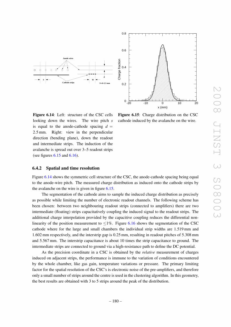
2008 JINST 3 S08003

Anode wires

Cathode stripsS W

S=d=2.5 mm

d

0

0.2

0.4

0.6

0.8

-20 -10 0 10 20x (mm)

Cha

rge

frac

tion

Figure 6.14: Left: structure of the CSC cellslooking down the wires. The wire pitch sis equal to the anode-cathode spacing d =2.5 mm. Right: view in the perpendiculardirection (bending plane), down the readoutand intermediate strips. The induction of theavalanche is spread out over 3–5 readout strips(see figures 6.15 and 6.16).

Figure 6.15: Charge distribution on the CSCcathode induced by the avalanche on the wire.

6.4.2 Spatial and time resolution

Figure 6.14 shows the symmetric cell structure of the CSC, the anode-cathode spacing being equalto the anode-wire pitch. The measured charge distribution as induced onto the cathode strips bythe avalanche on the wire is given in figure 6.15.

The segmentation of the cathode aims to sample the induced charge distribution as preciselyas possible while limiting the number of electronic readout channels. The following scheme hasbeen chosen: between two neighbouring readout strips (connected to amplifiers) there are twointermediate (floating) strips capacitatively coupling the induced signal to the readout strips. Theadditional charge interpolation provided by the capacitive coupling reduces the differential non-linearity of the position measurement to ≤1%. Figure 6.16 shows the segmentation of the CSCcathode where for the large and small chambers the individual strip widths are 1.519 mm and1.602 mm respectively, and the interstrip gap is 0.25 mm, resulting in readout pitches of 5.308 mmand 5.567 mm. The interstrip capacitance is about 10 times the strip capacitance to ground. Theintermediate strips are connected to ground via a high-resistance path to define the DC potential.

As the precision coordinate in a CSC is obtained by the relative measurement of chargesinduced on adjacent strips, the performance is immune to the variation of conditions encounteredby the whole chamber, like gas gain, temperature variations or pressure. The primary limitingfactor for the spatial resolution of the CSC’s is electronic noise of the pre-amplifiers, and thereforeonly a small number of strips around the centre is used in the clustering algorithm. In this geometry,the best results are obtained with 3 to 5 strips around the peak of the distribution.

– 180 –

2008 JINST 3 S08003

Figure 6.16: The segmentation of the CSCcathodes. The individual strip widths for thelarge and small chambers are b = 1.519 mmand 1.602 mm, respectively. The interstripgap is 0.25 mm, resulting in readout pitches ofa = 5.308 mm and 5.567 mm. The intermedi-ate strips contribute an additional charge inter-polation, improving the linearity of the recon-structed position. The intermediate strips arenot connected to readout electronics.

Figure 6.17: The inclination of the CSC’s to-wards the interaction point. Dimensions aregiven in mm.

The second most significant contribution to the spatial resolution of the CSC is the effect ofinclined tracks and the Lorentz angle. The charge interpolation is optimal when the avalanche isformed on a single point along the wire, while a significant extent of the anode charge results ina degradation. The spreading of the charge deposition can be caused by delta electrons, inclinedtracks and a Lorentz force along the wire, as the magnetic field is not collinear with the electric fieldaround the wire. While the effect of the Lorentz force cannot be corrected in a CSC, it does notlead to a systematic shift of the measured coordinate, but only to a slight reduction in resolution.The effect of inclined tracks is minimised by tilting the chamber towards the interaction point sothat infinite momentum tracks are normal at the centre of the chamber (figure 6.17).

The strips in the second cathode plane are parallel to the wires and measure the position ofthe avalanche in the non-bending φ -plane. The spacing of the readout strips is larger than the onein the bending η-plane (21 mm and 12.92 mm for large and small chambers, respectively) leadingto a resolution of about 5 mm.

– 181 –

2008 JINST 3 S08003

Table 6.7: Modularity of the CSC system and readout.Wires Strips Readout Strips Readout Total Front-end Front-end

channels channels readout chips boardsalong wires across wires channels

Plane small 250 48 48 574 192 240 10large 402 48 48 574 192 240 10

Chamber small 1000 192 192 2296 768 960 40 10large 1608 192 192 2296 768 960 40 10

One side 16 chambers 20864 3072 3072 36736 12288 15360 640 160System 32 chambers 41728 6144 6144 73472 24576 30720 1280 320

If more than one track is present in a given event, the pulse height is used to match themeasurements in the two projections. Because of the broad pulse height distribution in a gaschamber and the high resolution of the ADC’s, both tracks will have, in most of the cases, adifferent pulse height value, allowing for an unambiguous η/φ assignment of the tracks from theseparate measurements in η and φ . In the rare cases of near equality, the information from theother three chamber layers will be used. In using the information of all four chamber layers, theη/φ assignment for two or more tracks seems to be sufficiently robust.

The time resolution of the CSC is an important parameter for the correct tagging of the beam-crossing. The maximum drift path of a primary electron to the closest wire being only 1.27 mm, onewould expect a maximum drift time of about 20 ns, given the average drift velocity of 60 µm/ns.However, the vanishing drift field at the boundary between two cells creates regions of very lowdrift velocity leading to long tails in the distribution of the arrival times, which prevents reliabletagging of the beam-crossing. By OR-ing the signals of corresponding cathode strips in the fourchamber planes, the tails disappear, as virtually no track can pass close to a cell boundary in all fourlayers. The time of arrival distribution thus obtained is symmetric with an RMS value of 3.6 ns,resulting in a reliable tagging of the beam-crossing.

6.4.3 Mechanical design

The CSC’s are located at a distance of about 7 m from the interaction point. They are mountedtogether with the MDT’s and TGC’s on the shielding disk (see section 3.2) forming the so-calledsmall wheel and occupy the radial space between 881 mm and 2081 mm, corresponding to thepseudorapidity range |η |= 2−2.7.

The CSC’s come in two types of chambers as shown in figure 6.18 and are arranged in twodisks of eight chambers each, as shown in figure 6.13. Each chamber consists of four wire planesleading to a similar configuration like in the multi-layer of the MDT system, but with much finergranularity. The modularity of the CSC system is summarised in table 6.7.

The CSC design utilises low-mass materials to minimise multiple scattering and detectorweight. A four layer chamber is formed by five flat rigid panels, each made of an 18.75 mm thicksheet of polyurethane foam and two 0.82 mm thick copper-clad laminates, where the 17 µm thickcopper cladding forms the cathodes. Precision strips glued on the panels provide the 2.5 mm stepfor the anode wire plane. The anode wires have a diameter of 30 µm and are made of gold-platedtungsten with 3% rhenium.

– 182 –

2008 JINST 3 S08003

Figure 6.18: Shapes of large and small CSC’s. Dimensions are given in mm.

There are 250 and 402 wires per chamber plane along the bending direction in the small andlarge chambers, respectively (table 6.7). The readout pitch in the bending plane is 5.56 mm and5.31 mm for the small and large sectors respectively with a total of 192 channels per plane forboth. The odd strip width is the result of the different radial chamber lengths and the desire tofix the number of channels in multiples of 192. The transverse coordinate strips have widths of12.52 mm and 21.00 mm for the small and large chambers respectively with a total of 48 stripsper plane. The cathode strips are lithographically etched for highest precision. The five panels areprecisely positioned with respect to each other with the aid of locating pins. The outer copper-cladlaminates of each chamber form an electromagnetic shield for the detector. A cutout view of onegap formed by two panels is shown in figure 6.19. Signals from the precision cathode strips aredirectly connected to the front-end (ASM-I) boards located on the chamber edges. The transversecoordinate signals are transferred via short ribbon cables to similar front-end boards mounted onthe chamber frame (figure 6.20).

The 16 chambers of an end-cap are mounted onto precisely manufactured stainless steelframes which, in turn, are mounted on adjustable brackets of the small wheel structure.

6.4.4 Readout electronics

The CSC’s have to operate at the innermost part of the small wheel, a region which is charac-terised by a high density of detector components, difficult accessibility and high radiation levels.As standard components like CMOS-processors, FPGA’s or commercial ADC’s are not expectedto operate reliably in this environment, the readout electronics had to consist of custom-designedbuilding blocks, fabricated in radiation hard technologies, combining performance with simplicityand reliability. All other commercial components were radiation certified according to ATLAS

– 183 –

2008 JINST 3 S08003

Figure 6.19: Structure of the CSC.

Figure 6.20: Model of a CSC chamber with four planes showing the location of the readout elec-tronics.

requirements. To limit the number and complexity of custom components, the front-end function-ality had to be reduced to a minimum. The design therefore aimed at shifting the data as early aspossible, i.e. after the L1 trigger latency to the ROD’s in the shielded area in USA15.

The readout architecture of the CSC’s is shown in figure 6.21. At the first stage, the chambersignals are amplified and shaped (ASM-I). At the second stage, the pulse train is sampled at a rateof 40.08 MHz and is stored in a Switched Capacitor Array (SCA) while awaiting the L1 trigger

– 184 –

2008 JINST 3 S08003

Figure 6.21: Schematics of the CSC front-end electronics. Regions shaded in yellow representcustom-made ASIC’s.

decision. Upon arrival of a L1 trigger accept signal, the stored data are digitised, multiplexed andtransferred to the ROD.

A particularly demanding aspect of the centroid-finding system is to achieve an intercalibra-tion of < 0.5% between adjacent channels. This requires high stability of the front-end amplifiersand small leakage in the analogue storage system, as well as an appropriate calibration system.

Signal processing in the front-end chip, crucial for the system performance, is as follows.Subsequent to the charge-sensing pre-amplifier, the pulse-shaping stage consists of a seventh orderfilter providing a bipolar pulse with a 70 ns peaking time, to reject low-frequency noise and toassure a prompt return of the signal to the baseline. The choice of these parameters was based onan assumed maximum rate of about 600 kHz per strip at full LHC luminosity, including the usualsafety factor of 5. Pre-amplifier and shaper are realised as monolithics with 24 channels per chip.The 0.5 µm CMOS technology was used because of known reliability and high radiation tolerance.

Each CSC chamber has 768 readout channels in the precision (bending) and 192 in the trans-verse direction, so 32 and 8 chips (24 channels) are needed for the readout of both directions,respectively. A group of four chips is mounted on a printed circuit-board (ASM-I), such that the40 chips of a chamber are served by 10 ASM-I boards, which are mounted on the lateral frame ofthe CSC, see figure 6.20. Two ASM-I boards in turn are served by one ASM-II board which sendsthe signals to the off-detector electronics via optical fibres. A breakdown of components used inthe CSC readout is given in table 6.7.

The signals from the ASM-II boards are routed to the CSC ROD’s in the USA15 control room.The ROD’s are VME modules which perform zero suppression, discard signals with incorrecttiming, apply calibration constants and build event fragments to be sent to the TDAQ system. Theyalso provide control signals for the on-chamber electronics. ROD’s are interfaced to the front-endand to the TDAQ via transition modules which handle all data traffic via optical fibres.

Each ROD services two CSC’s and consists of 13 DSP-based generic processing units, whichcommunicate with the ASM-II’s (10), build event fragments (2) and handle the operation of theROD and the interface to the TDAQ (1). More details on the CSC readout are given in [196, 197].

– 185 –

2008 JINST 3 S08003

Figure 6.22: CSC resolution and efficiency in a high rate test.

An additional constraint for the construction of the readout system came from the fact thatnatural air convection is practically absent around the CSC’s, and so liquid cooling had to beprovided to evacuate the dissipated heat. Water cooling is implemented for the front-end electronicsof the CSC’s, using the leakless cooling technique developed for CERN experiments.

6.4.5 Performance of the CSC

The CSC’s have been tested under conditions as close as possible to those in the final experiment.For this, the Gamma Irradiation Facility at CERN has been used. In any tested chamber of four CSCplanes, two layers were used as reference for the track location while the other two were consideredthe devices under investigation. The intensity of the gamma background could be adjusted up to2 kHz/cm2. The results are shown in figure 6.22. Compared to zero background, the resolutiondegrades from ∼ 45 µm to 65 µm at 1 kHz/cm2, while the inefficiency of a single CSC layerincreases from ∼ 4% to 10%. The 10% inefficiency at 1 kHz/cm2 is acceptable, as the probabilityfor two or more layers to be inefficient in the same event is very low.

6.5 Alignment system of the precision chambers

In the ATLAS spectrometer, the MDT as well as the CSC chambers and their auxiliary alignmentobjects (alignment bars and reference system plates, see below) are installed with a precision ofabout 5 mm and 2 mrad with respect to their nominal positions. In contrast, the actual chamberlocations must be known to a precision of ≤ 30 µm in order to achieve the required momentumresolution: this is more than two orders of magnitude tighter than the positioning accuracy. Toreach this precision goal, an alignment system was built which relates the position of each chamberto that of its neighbours, both within an MDT layer and along R− z trajectories within MDTtowers. With the internal accuracy of the MDT’s guaranteed by construction, and their planaritymonitored by optical in-plane alignment sensors (see section 6.3.2), this alignment system forms adense, stable grid for monitoring (in the barrel) or reconstructing (in the end-cap) the position ofeach MDT wire in the muon system. A schematic representation of the alignment system in a large

– 186 –

2008 JINST 3 S08003

Figure 6.23: Principle of the alignment of the ATLAS muon spectrometer. See text for details.

sector is shown in figure 6.23. Due to different geometrical constraints, the alignment strategies aresomewhat different in the barrel and end-cap regions (section 6.5.1) and several specialised opticalalignment sensors have been developed (section 6.5.2). The overall system layout is detailed insection 6.5.3.

The optical alignment techniques described below are insufficient to reconstruct, on theirown, the absolute positions of the MDT barrel chambers: only variations in relative position canbe determined with the required precision. Track-based alignment algorithms must therefore beused in combination with the optical system to achieve the desired sagitta accuracy, and also todetermine the global positions of the barrel and end-cap muon-chamber systems with respect toeach other and to the inner detector, in the overall ATLAS reference frame (section 10.3.2). Amore extensive presentation of the alignment strategy and technical implementation can be foundin [198, 199].

6.5.1 Alignment strategies

In the barrel, the chambers inside a MDT row are referenced to each other by chamber-to-chamberalignment sensors (praxial and axial systems, see figure 6.23), while the projective system con-nects the inner, middle, and outer MDT layers, simulating the trajectories of an infinite-momentumtrack originating from the interaction point. This optical network is able to reliably detect relativechanges in chamber position at the 20 µm level. However, because of its essentially projectiveconfiguration, it remains insensitive to some specific geometrical distortions, and therefore unableto provide absolute chamber positions on its own. Additional optical lines (table 6.8) link MDTchambers to the barrel toroid cryostat, or relate adjoining chambers in large and small sectors.Once fully functional, the optical alignment system will provide a slightly overconstrained net-work of optical sensors which can determine the absolute chamber positions in the barrel regionto an accuracy of a few hundred microns, and yield a systematic uncertainty of 100− 200 µm on

– 187 –

2008 JINST 3 S08003

Table 6.8: The alignment components in barrel and end-cap. Three different types of imagingsystems are used, adapted to the special application: RASNIK (R), BCAM (B) and SaCam (S).The BIR and BIM chambers are shown in figure 6.1. See text for details.

Barrel alignment End-cap alignmentName Type Number Function Name Type Number FunctionIn-plane R 2110 MDT deformation In-plane R 1984 MDT deformationPraxial R 2006 MDT-MDT distance In-bar R 352 Bar deformationAxial R 1036 MDT-MDT planarity Radial B 96 Bar deformationProjective R 117 Tower alignment Polar B 208 Bar-bar linkReference S 256 Link to toroid Azimuthal B 736 Bar-bar linkCCC S 260 Small-large link Proximity R 2384 MDT-bar and MDT-MDT linkBIR-BIM R 32 BIR/BIM link Saloon door B 584 MDT-bar link

3D sensor B 192 CSC-bar and CSC-CSC linkTotal: 5817 Total: 6536

the residual sagitta. Because of mechanical positioning uncertainties on some optical sensors, theultimate 30 µm precision on the sagitta (but not necessarily on the absolute chamber positions), andin particular the exact reference values with respect to which relative changes are monitored, canonly be reached, in the barrel region, by combining optical and track-based alignment algorithms.

In the end-caps, the light path between the inner and the middle layer is obstructed by thecryostat vessels of the toroid magnets. The polar alignment therefore proceeds in two steps us-ing high-precision rulers (alignment bars), as an intermediate reference [200]. The polar (quasi-projective) optical lines connect the alignment bars installed in each EI, EM and EO layer; thechambers, in turn, are optically connected to their neighbouring bars by proximity sensors. Addi-tional sensor families, listed in table 6.8, determine the remaining degrees of freedom. Simulationshave demonstrated that this network is sufficiently precise and overconstrained to determine ab-solute chamber positions within each end-cap region to a 300 µm accuracy, and relative chamberpositions along muon trajectories to a 40 µm accuracy on the sagitta. Test-beam results and pre-liminary tests after installation of the EM layers in the ATLAS cavern have already demonstratedthat an alignment accuracy at about this level is reached.

The alignment bars in the EI wheel are also used for the alignment of the CSC’s. The positionsof the large CSC’s relative to these bars and the position of the small CSC’s relative to the largeones are measured with optical sensors, in a similar way as is done for the MDT’s. The alignmentprecision of the CSC’s is thus expected to be at the same level as for the MDT’s.

The relative positions of the barrel MDT system and of the forward end-cap chamber systemsmust also be known to a few tens of microns to ensure accurate momentum measurement for muonscrossing from one region to the other. Track-based alignment algorithms are being developed toprovide the required precision.

6.5.2 Optical alignment sensors

Three different optical systems are used in the ATLAS alignment: RASNIK’s, BCAM’s andSaCam’s. All three systems are based on the principle of a three point straightness monitor: an op-toelectronic image sensor (CCD or CMOS) monitors the position of an illuminated target through

– 188 –

2008 JINST 3 S08003

Figure 6.24: The RASNIK alignment system. The image sensor (RasCam) is a CMOS sensor inthe barrel and a CCD sensor in the end-cap. An infrared filter is placed in front of the sensorsto avoid stray light. A RasMux multiplexer is installed on each chamber, servicing up to eightRasCam sensors. A MasterMux can multiplex up to 16 RasMux’s, sending the data to the USA15hall for processing.

a lens. The sensor image is analysed online and converted into four parameters characterising thedeviation from the nominal geometry: two translations perpendicular to the optical axis, the rota-tion around and the longitudinal position along the axis, the latter being derived from the opticalmagnification.

Figure 6.24 shows a schematic of the RASNIK system, the most frequently used element ofthe muon alignment system. An image sensor (RasCam) monitors through a lens an illuminatedtarget carrying a chequer-board pattern imprinted on a mask. For a symmetric RASNIK with thelens halfway between image sensor and mask, a transverse resolution of 1 µm and a magnificationresolution of 2 × 10−5 have been obtained. A description of the RASNIK alignment system canbe found in [186] and [201].

The BCAM is a camera consisting of a CCD image sensor which monitors the position ofa laser diode through a lens. The BCAM housing also contains a set of two or four laser diodeswhich can be used as targets by another BCAM. BCAM’s are mostly used in pairs, facing eachother. The image sensor is placed close to the focal plane of the lens (76 mm), while the target withthe laser diodes is placed at a distance of 0.5 m to 16 m. The image of a laser diode on the CCDappears as a circular spot.

BCAM’s achieve a resolution of 5 µrad for a target distance of 16 m. If the target consistsof two or more laser diodes with a known separation, relative angles can be extracted, which yieldmagnification and rotation around the optical axis. If BCAM’s are used in pairs, the absoluteangular position of the partner can be determined with 50 µrad accuracy.

Like the BCAM, the SaCam consists of a camera with an image sensor and a lens at fixeddistance. The target consists of four back-illuminated holes, covered by a light diffuser. The lensis mounted at distances ranging from 25 mm to 80 mm, depending on the distance between imagesensor and target. A relative resolution of 5 µrad has been achieved with the SaCam, a result similarto that of the BCAM.

Another specialised sensor type is the 3D sensor, a pin-hole camera similar to the BCAM,which monitors the position of four laser diodes placed at two different distances along the opticalaxis. This sensor type is used for the alignment of the CSC’s.

– 189 –

2008 JINST 3 S08003

Figure 6.25: Layout of the optical-alignment lines (red) for three adjacent barrel sectors. See textand table 6.8 for details. The Chamber-to-Chamber Connector sensors (CCC) connect chambers ina small sector to those in an adjacent large sector.

Figure 6.26: Layout of the alignment of two MDT’s and CSC’s in the end-cap. Only alignmentsensors belonging to these sectors are shown, and the EE chambers and bars have been omitted.See text and table 6.8 for details.

– 190 –

2008 JINST 3 S08003

6.5.3 Layout of the alignment system

The alignment rays in three adjacent barrel sectors are shown in figure 6.25. The praxial sys-tems (two short, crossed RASNIK’s connecting adjacent chamber corners) and the axial systems(interleaved long RASNIK systems along the chamber) monitor the geometry of each row of sixchambers. The relative position of the chamber layers perpendicular to the polar direction is mon-itored by the projective rays. The projective system works with RASNIK’s, where BIL chambershold the mask, BML’s the lenses and BOL’s the image sensor. Chambers in the small sectors (BIS,BMS and BOS) are not equipped with projective lines and are referenced to the adjacent largechambers by Chamber-Chamber Connection sensor (CCC).

The layout of the alignment rays in the end-cap is shown in figure 6.26. The presence of thecryostat of the end-cap toroid magnet allows only for three polar lines per small sector, one of thempassing through a horizontal stay tube connecting the two outer flanges of the cryostat. To copewith this limitation, a grid of alignment bars using a quasi-projective alignment system was built.The chamber positions are referenced to this grid of aligned precision rulers. Each MDT wheelcarries eight bars, with lengths of up to 9.6 m, placed at the border between large and small sectors.The bar straightness and elongation are monitored by a set of internal, interleaved RASNIK’s andby a number of temperature sensors. Prior to installation, the geometry of each bar is carefullymeasured using a large coordinate measuring machine.

The bar positions in the grid are determined by a network of BCAM sensors measuring thebearing angle of light sources located on adjacent bars. Radial BCAM’s monitor the bar deforma-tion, azimuthal BCAM’s connect adjacent bars within a wheel, and polar BCAM’s connect bars ofdifferent wheels. MDT chambers are referenced to the alignment grid using RASNIK proximitysensors, where image sensor and lens are placed on the chamber, while the mask is on the neigh-bouring bar. In order to monitor chamber rotations around the bar axis, azimuthal BCAM’s alsolook at targets (the saloon-door sources) on the opposite edge of the adjacent MDT chamber. Thepositions of CSC chambers relative to the bars and to each other are measured by 3D sensors.

6.6 Trigger chambers

The trigger chambers of the muon system provide fast information on muon tracks traversing thedetector, allowing the L1 trigger logic to recognise their multiplicity and approximate energy range.The main requirements for the trigger system are:

• discrimination on muon transverse momentum;

• bunch-crossing identification;

• fast and coarse tracking information to be used in the high-level trigger stages;

• second coordinate measurement in the non-bending φ -projection to complement the MDTmeasurement, see section 6.2;

• robustness towards random hits due to n/γ-background in the experimental hall.

– 191 –

2008 JINST 3 S08003

The trigger detectors must provide acceptance in the range |η | ≤ 2.4 and over the full φ -range.This poses a considerable challenge to the design of the trigger system as resolution requirements inbarrel and end-cap are quite different, an obvious reason being that muon momenta, correspondingto a given pT , are strongly increasing with η . At |η |= 2.4, for example, p is about 5.8 times largerthan pT , while the integrated bending power is only about twice the value as at η = 0. This leadsto the necessity of an increased and η-dependent granularity in the end-cap trigger system, if thepT -resolution is to match the one in the barrel. The fact that the three trigger layers in the end-capare outside the magnetic field, seeing no curvature, and that their respective distances are smallerthan the ones in the barrel (figure 6.27) also calls for a finer granularity of the end-cap triggerreadout. Furthermore, radiation levels in the end-cap region reach a factor of 10 higher than inthe barrel. Another difficulty for end-cap triggering comes from the strong inhomogeneities of themagnetic field in the region 1.3≤ |η | ≤ 1.65 as can be seen in figure 2.10. In this transition region,the superposition of the fields of barrel and end-cap toroids leads to a complex field geometry withlarge field components in φ (the non-bending plane) and strong inhomogeneities of the integratedbending power, which in two locations in the η and φ plane is close to zero. In this angular region,all tracks are nearly straight, similar to tracks with very high momentum. In order to avoid highfake trigger rates, this region can be excluded from the trigger by a masking algorithm, which againcalls for a fine readout granularity to keep the resulting trigger losses to a minimum.

Figure 6.27: Schematics of the muon trigger system. RPC2and TGC3 are the reference (pivot) planes for barrel andend-cap, respectively.

Taking these constraints intoaccount, two different technologieshave been selected for barrel (|η | ≤1.05) and end-cap (1.05≤ |η | ≤ 2.4)regions. In the barrel, Resistive PlateChambers (RPC’s) are used due togood spatial and time resolution aswell as adequate rate capability. ARPC has no wires, which simpli-fies its construction and makes cham-bers less sensitive to small deviationsfrom planarity if appropriate spacersare used to keep the gap width con-stant. Being located in the compara-tively homogeneous field of the bar-rel toroid and having sufficient spac-ing between the three trigger layers(see table 6.9), RPC’s give sufficient trigger selectivity even with moderate channel count, i.e.spatial resolution.

In the end-cap region, Thin Gap Chambers (TGC’s) have been selected: they operate onthe same principle as multi-wire proportional chambers, and they provide good time resolutionand high rate capability. Their spatial resolution is mainly determined by the readout channelgranularity, which can be adjusted to the needs by wire ganging. TGC’s have demonstrated a highlevel of reliability and robustness in previous experiments.

To reduce the probability of accidental triggers caused by random combinations of convertedγ’s, the coincidence condition in both types of trigger chambers is established separately in the η

– 192 –

2008 JINST 3 S08003

Table 6.9: Segmentation of the RPC system in 544 chambers and 962 units (126 chambers aremade of only one unit). Columns 4 and 9 give the radial positions of the RPC stations, whilecolumns 5 and 10 give the distance to the pivot station (RPC2), relevant for the pT resolution. Alldimensions are in mm.

Small sector Large sectorName Units Chambers Location To Maximum Units Chambers Location To Maximum

in R pivot |z| in R pivot |z|RPC1 148 84 7820 545 9362 149 94 6800 678 9147RPC2 148 84 8365 9362 149 94 7478 9660RPC3 176 92 10229 1864 12847 192 96 9832 2354 12267Total 472 260 490 284

and φ -projection, a valid trigger requiring a coincidence of both. This also suppresses fake triggersfrom curling tracks, i.e. multi-MeV electrons from γ-conversions, spiralling in the magnetic field,potentially creating correlated hits in the trigger chambers. In the barrel, three layers of triggerchambers are implemented while in the end-cap a forth layer is added to increase the trigger ro-bustness in case of higher backgrounds. The schematic layout of the trigger system is shown infigure 6.27. In the barrel, two layers (RPC1 and RPC2) sandwich the MDT’s of the middle layer,while the third one (RPC3) is located close to the outer MDT layer. In the end-cap, the three layersare in front (TGC1) and behind (TGC2 and TGC3) the second MDT wheel, while the fourth layeris located in front of the innermost tracking layer. The trigger information is generated by a systemof fast coincidences between the three last layers along the trajectory of the muon particle. Eachcoincidence pattern corresponds to a certain deviation from straightness, i.e. curvature of the track,which is used as a criterion for the track to have passed a predefined momentum threshold.

The deviation from straightness is the deviation of the slope of the track segment betweentwo trigger chambers from the slope of a straight line between the interaction point and the hit ina reference layer called the pivot plane, which is the second layer in the barrel (RPC2) and thelast layer in the end-cap (TGC3), as illustrated in figure 6.27. For the low (high)-pT trigger in thebarrel, for example, the slope between RPC2 and RPC1 (RPC3) is compared to the slope betweenthe interaction point and RPC2.

To assure full acceptance down to the low-momentum limit, the trigger chambers have regionsof overlap with adjacent chambers and between the barrel and end-cap regions. As this may causedouble counting of tracks leading to fake two-muon triggers, algorithms are in place to treat theseoverlap regions, either within the barrel or end-cap trigger logic, or as a part of the muon interfaceto the central trigger processor, see section 8.2.2.3. An overview of the muon trigger chambers isgiven in [202, 203] and details about the coincidence system and readout logic are given in [204].

6.7 Resistive plate chambers

The trigger system in the barrel consists of three concentric cylindrical layers around the beamaxis, referred to as the three trigger stations. Figure 6.28 shows a standard barrel sector and thelocation of the RPC’s (coloured) relative to the MDT’s. The large lever arm between inner andouter RPC’s permits the trigger to select high momentum tracks in the range 9–35 GeV (high-pT trigger), while the two inner chambers provide the low-pT trigger in the range 6–9 GeV. Thechamber count and radial position of the RPC’s are given in table 6.9. Each station consists of two

– 193 –

2008 JINST 3 S08003

Figure 6.28: Cross-section through the upper part of the barrel with the RPC’s marked in colour.In the middle chamber layer, RPC1 and RPC2 are below and above their respective MDT partner.In the outer layer, the RPC3 is above the MDT in the large and below the MDT in the small sectors.All dimensions are in mm.

independent detector layers, each measuring η and φ . A track going through all three stations thusdelivers six measurements in η and φ . This redundancy in the track measurement allows the useof a 3-out-of-4 coincidence in both projections for the low-pT trigger (RPC1 and RPC2 stations)and a 1-out-of-2 OR for the high-pT trigger (RPC3 station). This coincidence scheme rejects faketracks from noise hits and greatly improves the trigger efficiency in the presence of small chamberinefficiencies.

The naming scheme of the RPC’s is identical to the one in the MDT’s, a RPC in a small sectorof the middle layer thus being called a BMS. To denote a RPC/MDT pair in the outer layer the termstation is used, while for the RPC/MDT/RPC packages in the middle layer the term superstationsis used.

6.7.1 Principle of operation

The RPC is a gaseous parallel electrode-plate (i.e. no wire) detector. Two resistive plates, madeof phenolic-melaminic plastic laminate, are kept parallel to each other at a distance of 2 mm byinsulating spacers. The electric field between the plates of about 4.9 kV/mm allows avalanches toform along the ionising tracks towards the anode. The signal is read out via capacitive couplingto metallic strips, which are mounted on the outer faces of the resistive plates. The gas used is amixture of C2H2F4/Iso-C4H10/SF6 (94.7/5/0.3) which combines relatively low operating voltage

– 194 –

2008 JINST 3 S08003

Table 6.10: RPC parameters and performance.

Parameter Design valueE-field in gap 4.9 kV/mmGas gap 2 mmGas mixture C2H2F4/Iso-C4H10/SF6 (94.7/5/0.3)Readout pitch of η and φ -strips 23–35 mmDetection efficiency per layer ≥98.5%Efficiency including spacers and frames ≥97%Intrinsic time jitter ≤1.5 nsJitter including strip propagation time ≤10 nsLocal rate capability ∼1 kHz/cm2

Streamer probability ≤1%

(due to the low SF6 concentration), non-flammability and low cost, while providing a comfortableplateau for safe avalanche operation. The main parameters and performance of the RPC’s are givenin table 6.10 and further details on the parameters in [176].

RPC’s can be operated both in avalanche and streamer mode. In the high background envi-ronment encountered at the LHC, the avalanche mode offers the benefit of higher rate capabilityand rate-independent time resolution and has therefore been selected as the operation mode. At thenominal operating voltage of 9.8 kV, a signal with a width of about 5 ns is generated by the trackwith a streamer probability of less than 1%.

The small jitter of the RPC signal in avalanche mode with respect to the passage of theparticle is due to the primary electrons not having to drift to a region of amplification, as is the casein all types of wire chambers. In the strong and uniform electric field inside a RPC cell, all primaryelectron clusters form avalanches simultaneously, producing one single signal instantaneously afterthe passage of the particle. The charge multiplication in each avalanche continues until its arrivalat the anode plane and, therefore, the gas gain of each avalanche depends on the distance of theprimary cluster from the anode. The total signal charge is thus dominated by the few clustersproduced at the largest distances from the anode. The RPC operating parameters are discussedin [205–207].

6.7.2 Mechanical structure

A RPC trigger chamber is made of two rectangular detectors, contiguous to each other, called units.Each unit consists of two independent detector layers, called gas volumes, which are each read outby two orthogonal sets of pick-up strips.

The structure of the gas volumes (i.e. 1/2 unit) is identical for all RPC’s (figure 6.29): tworesistive plates (plastic laminate, 2 mm) with a volume resistivity of 1010 Ωcm, delimit a gas gapof 2 mm, the correct distance being assured by a series of insulating spacers. The outside surfaceof the resistive plates is coated with a thin layer of graphite paint (100 kΩ/) to assure the HVand ground connection of the resistive electrodes. The graphite electrodes are insulated from the

– 195 –

2008 JINST 3 S08003

Figure 6.29: Cross-section through a RPC, where two units are joined to form a chamber. Each unithas two gas volumes supported by spacers (the distance between successive spacers is 100 mm),four resistive electrodes and four readout planes, reading the transverse and longitudinal direction.The sandwich structure (hashed) is made of paper honeycomb. The φ -strips (measuring the φ

coordinate) are in the plane of the figure and the η-strips are perpendicular to it. Dimensions aregiven in mm.

pick-up strips by means of PET films (190 µm), glued to the graphite surfaces. The pick-up stripsoutside the PET layers are bonded on polystyrene plates (3 mm) and connected to the front-endelectronics. The outside surface of the polystyrene plates carries a copper sheet for grounding. Areadout signal is induced on the strips by the drift motion of the avalanche electrons. The graphiteelectrode interposed between the gas gap and the strips does not shield the induction in a significantway due to the graphite electrode’s high resistivity and the fast rise-time of the signal.

Each RPC unit is thus made of two detector layers (i.e. gas volumes) and four readout strippanels. The detector layers are interleaved with three support panels made of light-weight paperhoneycomb (40 kg/m3) and are held in position by a solid frame of aluminium profiles. The twoexternal support panels interconnected by the aluminium profiles give the required stiffness to thechamber. The BOL chambers being the largest size ones have a reinforced structure using alu-minium plates (2 mm) and aluminium honeycomb. The total thickness of a RPC unit with two gasvolumes, support panels and aluminium covers is 96 mm (106 mm for the BOL) and increases to112 mm (122 mm for the BOL) if the lateral profiles are included. The two units forming a cham-ber have an overlap region of 65 mm to avoid dead areas for curved tracks. The BMS gas volumeshave no physical segmentation in the transverse (φ ) direction, and thus cover the chamber overits full length. All other standard chambers, whose size exceeds the maximum length (3200 mm)of the available plastic laminates have gas volumes divided in two segments along the φ directionwith a 9 + 9 mm inefficient region in between due to the edge frames. The readout-strip panelsare also segmented in the longitudinal (φ ) direction, including the case of the BMS, in order to get

– 196 –

2008 JINST 3 S08003

an homogeneous trigger scheme for all chamber types. This reduces the η-strips time jitter by afactor of two. RPC’s have been certified for high rate operation and ageing at the GIF facility atCERN [208, 209].

All standard RPC’s, as listed in table 6.9, are assembled together with a MDT of equal di-mensions in a common mechanical support structure. In order to avoid constraining forces amongstthe two chamber types, light-weight kinematical supports were used, holding the chambers withminimum clearance as required by the confined radial space.

A number of small RPC chambers (special RPC’s) not paired with MDT’s are used aroundthe magnet ribs and in the feet region, where MDT’s cannot be installed because of lack of space.RPC’s, requiring less space, are used in these regions to keep the trigger acceptance loss to aminimum.

6.7.3 Signal path and readout electronics

Figure 6.30: Layout of a RPC readout stripplane.

A RPC operating in the avalanche mode producessignals of 5 ns full width at half-maximum witha time jitter of 1.5 ns. To preserve this high in-herent precision, the pick-up strips must be high-quality transmission lines with low attenuation,terminated at both ends with the characteristicimpedance.

The layout of a readout strip plane isshown in figure 6.30. The strips with a widthof 25–35 mm consist of 17 µm copper on a190 µm PET foil glued on a 3 mm plate of rigidpolystyrene, which is covered, on the outside, by50 µm PET and 17 µm copper as ground refer-ence. The strips are separated by a 2 mm gap witha 0.3 mm ground strip at the centre for improveddecoupling. This sandwich structure creates animpedance of about 25 Ω for the strips, slightlydepending on the width.

The front-end circuit is a three-stage shaping amplifier followed by a comparator. It is im-plemented in a eight-channel GaAs die (in order to avoid the encapsulation cost) which is bondedwith 20µm-diameter gold wire on a printed board serving eight strips. The boards are mountedalong the edges of the readout panels as shown in figure 6.30 and soldered directly to the stripsthus avoiding the introduction any further insensitive area in addition to those already contained inthe gas volume. While this prevents exchange of faulty amplifiers in the field, the known reliabilityof GaAs-ASIC’s minimises the risk of losing readout channels during the experiment.

The frequency response of the GaAs-amplifiers has a maximum at 100 MHz and a 60 MHzbandwidth, well adapted to the rise time of the chamber signals. The front-end electronics inputis coupled to the strips with a transformer integrated in the printed circuit matched to the signalpolarities of η and φ -strips, which are opposite to each other. The voltages defining the thresholds

– 197 –

2008 JINST 3 S08003

Table 6.11: Location and radial extension of the TGC wheels. All dimensions are in mm.

EM big wheel I layerM1 M2 M3 FI (small wheel) EI

triplet doublet doublet doublet doubletOverall centre in z 13440 14733 15153 6983 7370Inner radial extent 1900 2526 2610 2170 4700Outer radial extent 10682 11917 11917 4434 6190

of the comparators are supplied by external digital-to-analogue converter units, located in racks inthe experimental hall controlled via the DCS. Details of the RPC front-end electronics are givenin [210, 211].

The front-end output signals of the φ -strips are wired OR-ed such that two physical stripsform a logical strip of twice the length but with the same time jitter as a single strip. This is doneto avoid unnecessary granularity and to adapt the RPC readout segmentation to the trigger sectorsegmentation as discussed in section 8.2.2. The φ -strip length and the relative time jitter is onaverage about half that of an η-strip, giving the φ -strips a more precise timing.

In order to be used for the trigger, a signal from a RPC has to be compared with those inthe two other RPC’s along the path of the particle, i.e. in the same sector and tower, a task whichis accomplished by a system of fast coincidence units close to the chambers. Thus, coincidencesbetween strips in RPC1 and RPC2 are used to create the low-pT trigger. A high-pT trigger requireshits in all three trigger stations: RPC1 and RPC2 must fulfil the low-pT condition and a confirminghit must be found in RPC3. The inclusion of the low-pT trigger condition in the high-pT triggerdefinition leads to more robustness against fake triggers compared to a simple coincidence betweenRPC3 and only one inner RPC station. A detailed discussion of the RPC trigger system is given insection 8.2.2.1.

6.8 Thin gap chambers

6.8.1 Introduction

Thin Gap Chambers (TGC’s) provide two functions in the end-cap muon spectrometer: the muontrigger capability and the determination of the second, azimuthal coordinate to complement themeasurement of the MDT’s in the bending (radial) direction. The middle layer of the MDT’s inthe end-cap (EM-wheel) is complemented by seven layers of TGC’s, while the inner (I) layer iscomplemented by only two layers. The inner layer is segmented radially into two non-overlappingregions: end-cap (EI) and forward (FI, also known as the small wheel). EI TGC’s are mounted onsupport structures of the barrel toroid coils.

The azimuthal coordinate in the outer MDT wheel (EO), i.e. the coordinate along the tube, isobtained by the extrapolation of the track from the middle layer, which can be done accurately dueto the lack of magnetic field between EM and EO.

– 198 –

2008 JINST 3 S08003

The radial, bending coordinate is measured by the TGC wire groups, the azimuthal coordinateby the radial strips. The TGC’s need good time resolution to tag the beam-crossing with highefficiency (≥ 99%) and fine granularity to provide a sufficiently sharp cut-off in the momentum ofthe triggering muon. To match the granularity to the required momentum resolution, the size ofthe wire groups varies from 6 to 31 as a function of η , corresponding to a variation in width from10.8 mm to 55.8 mm. The alignment of wire groups in consecutive layers is staggered to optimisethe position resolution for a given number of electronics channels. The radial strips are staggeredin a similar way to achieve an azimuthal granularity of 2–3 mrad, as seen from the interaction point.

Figure 8.9 shows a longitudinal cut through the end-cap. TGC’s are located in the innermostlayer (marked I) and in the middle layers (EM-wheels marked M1–M3, corresponding to TGC1–3).The location of the MDT in a small (S) and large sector (L) are shown for reference. The locationalong z and the radial extension of the TGC wheels are given in table 6.11. A detailed listing of allrelevant construction parameters is given in the TGC parameter book [212].

6.8.2 Principle of operation

1.8 mm

1.4 mm

1.6 mm G-10

50 µm wire

Pick-up strip

+HV

Graphite layer

Figure 6.31: TGC structure showing anodewires, graphite cathodes, G-10 layers and a pick-up strip, orthogonal to the wires.

The main operational parameters of the TGC’sare summarised in table 6.12.

TGC’s are multi-wire proportional cham-bers with the characteristic that the wire-to-cathode distance of 1.4 mm is smaller thanthe wire-to-wire distance of 1.8 mm, as shownin figure 6.31. With a highly quenchinggas mixture of CO2 and n-C5H12 (n-pentane),this cell geometry allows for operation in aquasi-saturated mode, i.e. with a gas gain of∼ 3×105. This relatively low gas gain, com-pared to previous implementations of the TGCconcept, does not allow to make full use ofits independence from the primary ionisation.Some of its characteristics are still kept, evenat such a low gas gain. In particular:

• The highly quenching gas prevents the occurrence of streamers in all operating conditions.

• The pulse height observed in the interaction of low energy neutrons (1–10 MeV) is only afactor 30 larger than for a minimum ionising particle.

The high electric field around the TGC wires and the small wire-to-wire distance lead to very goodtime resolution for the large majority of the tracks. Only tracks at normal incidence passing midwaybetween two wires have much longer drift times due to the vanishing drift field in this region. Thiseffect was already discussed in the context of the CSC’s which have a similar cell geometry, seesection 6.4.2. In the TGC wheels, however, the angle of incidence for tracks emerging from the

– 199 –

2008 JINST 3 S08003

Table 6.12: Main TGC operational parameters.

Parameter Design valueGas gap 2.8 ± 0.10 mmWire pitch 1.8 ± 0.05 mmWire diameter 50 µmWire potential 2900 ± 100 VOperating plateau 200 VGas mixture CO2/n-pentane (55/45)Gas amplification 3×105

interaction point will always be greater than 10, thus a part of the track will be outside of the lowfield region. Including the variation of the propagation time on wires and strips, signals arrive with99% probability inside a time window of 25 ns.

6.8.3 Mechanical structure

The seven detector layers in the middle layers (big wheels, see section 9.5) are arranged in onetriplet and two doublets. The triplet is to cope with false coincidences from background hits, whichare more likely in the end-cap region than in the barrel.

The trigger detectors, forming circular disks, are mounted in two concentric rings, an outer orend-cap one covering the rapidity range 1.05≤ |η | ≤ 1.92 and an inner or forward one covering therapidity range 1.92≤ |η | ≤ 2.4. Figure 6.32 shows the cross-section of a TGC triplet and doublet.The structure consists of wire planes (anode), cathode planes, strip planes, shields and honeycombsupport structures. The cathode planes consist of 1.6 mm thick FR4 (Flame Resistant 4) plates,graphite coated on the inside, i.e. facing the wires, and with copper cladding on the other side.The resistivity of the graphite is of 1 MΩ/ in the end-cap and of 0.5 MΩ/ in the inner/forwardregion. Two of the copper layers in the triplet and doublets are segmented into readout strips to readthe azimuthal coordinate (marked “Cu strips” in figure 6.32). The solid copper layers serve as DCgrounds, while the segmented ones, being connected to amplifiers, are virtual grounds for the wiresignals. On the outside of the triplet and doublet chambers the honeycomb stiffeners are covered by0.5 mm thick FR4 plates for rigidity and mechanical protection. The adjacent chambers in a module(three in a triplet, two in a doublet) are separated by a 20 mm thick honeycomb paper stiffener.

A gas volume containing a wire plane and two cathodes is called a chamber, while the entiretyof three or two chambers in a triplet or doublet arrangement is called a unit. In the outer ring fouror five chambers in triplet and doublets, respectively, are mounted in the way of a ladder formingmodules. All TGC’s in the big wheel (EM) are segmented into 12 sectors of 30 in the azimuthaldirection. Thus, a sector in the outer ring comprises four modules of 7.5, while the inner ringhas two modules of 15. Altogether there are 744 units in the big wheels, corresponding to 1704chambers. The TGC wheel in the innermost layer has a slightly different geometrical structure,containing 45 units and 90 chambers on each side. A summary of the TGC segmentation is givenin table 6.13.

– 200 –

2008 JINST 3 S08003

Figure 6.32: Cross-section of a TGC triplet and doublet module. The triplet has three wire layersbut only two strip layers. The dimensions of the gas gaps are enlarged with respect to the otherelements.

Table 6.13: TGC modularity. Each wheel consists of 12 sectors, each sector containing an inner(forward) and an outer (end-cap) part, having a different azimuthal segmentation. A module covers15 in azimuth in the inner and 7.5 in the outer part.

EM big wheel I layer TotalM1 triplet M2 doublet M3 doublet I doublet

Modularity Inner Outer Inner Outer Inner Outer Inner OuterModules/sector 2 4 2 4 2 4Units/module 1 4 1 5 1 5Chambers/unit 3 3 2 2 2 2Units/sector 2 16 2 20 2 20Units/side 24 192 24 240 24 240 24 21 789Units/system 48 384 48 480 48 480 48 42 1578Chambers/sector 6 48 4 40 4 40Chambers/side 72 576 48 480 48 480 48 42 1794Chambers/system 144 1152 96 960 96 960 96 84 3588

All TGC units are enclosed on their periphery by a gas-tight envelope which is continuouslyflushed by CO2. This is done to keep a dry atmosphere in the region where the HV elements arelocated as well as to dilute any potential leak of the operating gas (n-pentane). If traces of thisflammable gas are detected in the CO2 stream at the output of the chambers, HV and LV as well asgas supplies are automatically switched off, and an alarm is activated.

6.8.4 Signal path, readout, and detector controls

The data flow starting with the primary wire and strip signals is as follows. After amplification inthe front-end amplifiers, signals are time-aligned and synchronised to the beam-crossing frequency.The subsequent signal processing makes use of the redundancy of the track measurement in the

– 201 –

2008 JINST 3 S08003

TGC layers to mitigate the effects of chamber inefficiencies and improve rejection of fake triggerscaused by background or noise hits. Thus the three signals of the triplet are combined to form a 2-out-of-3 coincidence, while the four signals of the two EM-doublets form a 3-out-of-4 coincidence.Track segments which have passed this early filter are forwarded to the coincidence matrix, whichperforms a fast search for signal coincidences corresponding to muon tracks in a certain momentumrange. A detailed description of the algorithm used and of the signal processing in the higher levelsof the trigger system is given in chapter 8.

The detector control system (DCS) is fully integrated into the trigger electronics. For theTGC, its role is not only of monitoring operating parameters like temperatures, voltages and cur-rents as well as the relative alignment of the detectors (down to 0.2 mm), but it can also initialiseits various elements. Furthermore, by combination with a special trigger signal of the patch-panelboard, it can monitor the charge left by an ionising particle in every chamber, and therefore act asa gas monitor for every single detector.

6.9 Commonalities in the muon system

6.9.1 The gas supplies in the muon system

While gas mixtures and operating conditions in the sub-systems of the muon spectrometer arequite different, being adapted to the requirements of the four chamber types, there are also manycommonalities amongst them from an operational point of view.

• The gases must be circulated in a closed loop system (mainly for cost reasons), except forthe CSC’s. This requires a complex recuperation and re-mixing system, using specialisedpurifiers to clean the gas before recirculation into the supply system. For safety and spacereasons, all recuperation systems are housed on the surface, requiring tight pressure and flowcontrol for the transfer to the underground experimental area.

• Distribution of the gas in the experimental cavern needs a high degree of modularity to beimmuned to leaks in any given supply line. Because of the considerable hydrostatic pres-sure variations along the height of the hall (25 m), pressure regulation has to be segmentedaccordingly. Therefore, gas distributors (racks) are located at three different levels in thegalleries and wheels of the detector each one supplying chambers in a±3 m range of relativeelevation.

• The flow rate in the gas distribution branches must be supervised by a correspondingly largenumber of flow and pressure meters for control of gas circulation (purity), operating pressureand leak detection. Precise pressure control is most important for CSC, RPC and TGC cham-bers, where operation is defined at ∼ 2 mb above the outside pressure at the correspondingheight and where a significant overpressure might lead to the destruction of the chamber.While this is not the case for the MDT’s, they also need precise pressure control for reasonsof drift time and gain stability.

Besides these commonalities there are many differences due to the particularities of the gases usedin each system. The high flammability of the TGC gas mixture, for example, requires stringent

– 202 –

2008 JINST 3 S08003

Table 6.14: Main characteristics of the muon gas supply systems.Characteristic MDT CSC RPC TGC

Gas mixture Ar/CO2/H2O Ar/CO2 C2H2F4/Iso-C4H10/SF6 CO2/n-pentaneComposition 93/7/(≤ 1000 ppm) 80/20 94.7/5/0.3 55/45Gas gain 2×104 6×104 107 3×105

Flammability — — low highOperating pressure (bar) 3 1 1 1Volume at operating pressure (m3) 710 0.5 14 16Gas exchanges/day 1 10 20 4Flow at operating pressure (m3/h) 30 0.2 12 2.7

safety precautions, the outside of the TGC’s being constantly flushed with CO2 in a separate, closedgas circuit. The return gas is monitored for traces on n-pentane, which could point to leaks in theprimary distribution system.

The main characteristics of the four gas supply systems are summarised in table 6.14 and inmore detail in table 9.5.

6.9.2 Electronics services and power consumption

The segmentation of the electrical services of the muon system follows the structure of the detectorwhich is characterised by a high level of modularity, consisting of electrically independent cham-bers. The service architecture aims to match this modularity in order to limit data loss in case agiven supply channel should fail. Power supply channels are kept floating i.e. the ground outputs ofthe power supplies are not connected amongst each other nor to the power supply housing or to anylocal safety ground. This way, the return current of a given chamber has only one path to return toits power supply. Ground loops (multiple ground returns) are therefore not possible. Ground loops,if present, might create noise coupling between near-by chambers and would expose the readout tonoise pick-up from sources in the ATLAS electrical environment. To further prevent pick-up, alllow-voltage (LV) supply cables are shielded by a copper mesh enclosing the cable wires. The cableshield is connected only at one end (chamber side) to the return wire.

For the definition of the DC level and for safety reasons all chambers are connected from onepoint of the chamber to the ATLAS structure ground. This star grounding does not allow currentsto circulate, i.e. does not create ground loops.

For cost reasons, the maximum supply modularity could not be maintained. Thus, every twoMDT chambers are supplied from one LV supply channel. The segmentation of the MDT high-voltage (HV) supplies is finer, with each multi-layer of three (four) tube layers being supplied by aseparate channel. Close to the chamber, a passive HV-split is installed (splitter box) to supply eachtube layer with an independent cable. In case of shorted tubes (broken wire), the correspondingtube layer can be disconnected, while the other layers would continue to work. Under normal LHCconditions and at an operating voltage of 3080 V, typical chamber currents are around 100 µA,yielding a negligible heat dissipation of about 0.3 W/chamber. The total LV power consumption ofthe MDT system is about 38.5 kW. Only one 4.5 V supply line is needed for each MDT chamberwith an average consumption of about 25 W.

– 203 –

2008 JINST 3 S08003

The CSC LV system supplies one voltage of 9 V. The operating voltages of 3.3 V and 5 Vare derived with radiation tolerant regulators close to the chamber. Each of the 16 chambers of anend-cap consumes about 40 A, leading to a total consumption of about 11.5 kW for both end-caps.The power dissipated in the readout electronics, is evacuated by a water cooling system. The RPC’shave separate LV supplies for the analogue front-end and the digital (trigger) electronics, operatingat -5 V and 3.3 V, respectively. A third voltage of -2 V is needed to supply the wired-ORs (pulldown voltage), combining two aligned physical wires into a “logical” wire. A number of referencevoltages are supplied to each chamber to define the discriminator thresholds for the ASD boards.The total power consumption of the RPC system is about 42 kW. The HV for the RPC’s (9.8 kV)requires one channel for each gas gap. To limit the required number of primary supply channels,splitter boxes are used, which are able to safely handle voltages up to 15 kV.

All power supply channels for the MDT barrel, the CSC’s, RPC’s and TGC’s in the small(EI) wheel are housed in racks in the UX15 experimental hall and have been certified for toleranceto radiation and magnetic field. The TGC chambers and the MDT in the big wheel (EM wheel) aresupplied from racks directly mounted on the wheel structure (non-standard “mini-racks”, due tospace limitations at the circumference of the EM wheel) in order to limit cable lengths and powerloss on the LV cables.

The TGC’s, like the RPC’s, have separate LV supplies for analogue and digital readout elec-tronics. The segmentation of the supplies in the EM wheel follows that of the TGC’s, with 12 sec-tors per side. For the small wheel there is only one supply channel per side for each voltage. TheHV modularity provides one supply channel per chamber with the exception of the 144 inner cham-bers in the M1 triplet which have two supply channels per chamber. A total of 3732 HV channelsare therefore used to serve the 3588 chambers of the TGC system.

Services for the small wheel, containing MDT’s, CSC’s and TGC’s, are routed through a flex-ible support structure (cable chains). When the small wheel is moved along the z-direction to giveaccess to the calorimeters and inner detector, most service channels will not require interruption,reducing access time and minimising the risk of damage to the small wheel chamber operation.

An overview of the segmentation and power consumption of the four muon sub-systems isgiven in table 6.15.

– 204 –

2008 JINST 3 S08003

Table 6.15: Power consumption of the four sub-systems of the muon spectrometer. Voltages deliv-ered by the power supplies (column 2) are approximate, depending on cable length and conductorcross-section. The differences between power supplied and consumed are due to cable losses aswell as losses in voltage regulators, used to stabilise voltages on the board. The aim of the cablinglayout was to limit cable losses to about 15–20% of the power used by the circuits. This could notbe achieved for the CSC’s due to limitations on cross-sections for supply cables. The PS-boardsand HS-crates are components of the TGC digital readout (see section 8.2.2).

Voltage Voltage Supply Average Average Total powerat power on channels current power (both sides)supply circuit per channel per channel consumed supplied

V V Number A W kW kWMDT- mezzanine cards & CSM 4.5 3.3 1140 7.5 25 28.2 38.5CSC (ASM-I & ASM-II)- analogue front-end 9 3.3 32 5 17 0.5 1.4- digital read-out 9 5 32 35 175 5.6 10.1RPC- analogue front-end -6.7 -5 528 4 20 10.6 14.2- wired-OR (pull-down) -2.3 -2 408 0.2 0.4 0.2 0.2- splitters & PAD boards 4.3 3.3 400 16 53 21.1 27.5TGC EM wheel- analogue front-end 3.3 3 24 217 651 15.6 17.2- analogue front-end -3.3 -3 24 56 168 4.0 4.4- readout (PS-boards) 3.4 3.3 24 55 182 4.4 4.5- readout (HS-crates) 3.3 3.3 24 34 112 2.7 2.7TGC EI wheel- analogue front-end 3.5 3 2 80 240 0.5 0.6- analogue front-end -3.5 -3 2 18 54 0.1 0.1- readout (PS-boards) 3.3 3.3 2 25 83 0.2 0.2Total power muon spectrometer 94 122

– 205 –

2008 JINST 3 S08003

Chapter 7

Forward detectors

In addition to the main ATLAS detector systems described in the previous chapters, three smallersets of detectors are being built to provide good coverage in the very forward region [213].

Ordered according to their distance from the interaction point as shown in figure 7.1, the firstsystem is a Cerenkov detector called LUCID (LUminosity measurement using Cerenkov Integrat-ing Detector, see section 7.1). LUCID is the main relative luminosity monitor in ATLAS and islocated at a distance of ±17 m from the interaction point, near the TAS (Target Absorber Secon-daries) collimator. The second system is the Zero-Degree Calorimeter (ZDC), located at a distanceof ±140 m from the interaction point (see section 7.3). This corresponds to the location wherethe LHC beam-pipe is divided into two separate pipes. The ZDC is embedded in the TAN (TargetAbsorber Neutral), located between the beam-pipes just after the split. The ZDC’s primary pur-pose is to detect forward neutrons in heavy-ion collisions. The most remote detector is the absoluteluminosity detector ALFA (Absolute Luminosity For ATLAS, see section 7.2). ALFA consists ofscintillating-fibre trackers located inside Roman pots at a distance of approximately ±240 m fromthe interaction point. Additional proton-tagging detectors are being considered at an even greaterdistance of about ±420 m [214] from the interaction point. These detectors, together with newradiation hard-detectors at ±220 m [215] are part of a possible upgrade programme.

7.1 The LUCID detector

Luminosity can be measured by several detectors in ATLAS, but LUCID (LUminosity measure-ment using Cerenkov Integrating Detector) [213] will be the only detector which is primarily ded-icated to online luminosity monitoring. LUCID is a relative luminosity detector. Its main purposeis to detect inelastic p-p scattering in the forward direction, in order to both measure the integratedluminosity and to provide online monitoring of the instantaneous luminosity and beam conditions.Potentially, LUCID could also be used for diffractive studies, for example as a rapidity-gap veto oras a tag for a diffractive signal [216].

During the initial period of LHC operation, the absolute calibration procedure for LUCID willuse calculations based on LHC machine parameters, initially determining luminosity to a precisionof ∼ 20−30%. Physics processes can also be used, such as W and Z counting [217] and exclusivemuon pair production via two-photon interactions [218]. The most accurate calibration will be

– 206 –

2008 JINST 3 S08003

Q1 Q2 Q3 D1 D2 Q4 Q5 Q6IP TAS

TAN

beam 2

beam 1

Dumpresistor boxes

17m

140 m

237m 4m

LUCID ZDCALFA

Figure 7.1: Placement of the forward detectors along the beam-line around the ATLAS interactionpoint (IP). See text for details.

obtained with the ALFA detectors which measure elastic Coulomb scattering. The goal is thus tomeasure the luminosity with an uncertainty of better than 5%.

At the LHC design luminosity, most bunch-crossings will result in multiple p-p interactions.The number of interactions per beam-crossing must be known in order to determine luminosity.LUCID is based on the principle that the number of interactions in a bunch-crossing is proportionalto the number of particles detected in this detector. This holds true even when most of the detectedparticles originate from secondary interactions.

The main requirements for the LUCID detector are:

• good acceptance for minimum-bias events;

• sufficient time resolution to measure individual bunch-crossings which occur every 25 ns;

• resistance to very high radiation levels;

• the ability to count individual charged particles;

• pointing capability in order to suppress signals from tracks which do not point to the inter-action point.

The concept of a luminosity detector consisting of an array of Cerenkov tubes (cones) wasdeveloped by the CDF collaboration [219]. The main challenges in using this type of detector at theLHC are the much higher radiation and background levels. ATLAS has approved the constructionof a detector with a reduced number of readout channels for the initial low-luminosity phase of theLHC operation (up to few 1033 cm−2 s−1), with a view to then possibly upgrade the detector to alarger coverage if it can be demonstrated through further studies that the detector would work wellat the LHC design luminosity.

Since there is no Landau tail in the measurement of Cerenkov light, it is in principle possibleto determine the number of particles which have entered a Cerenkov tube by using pulse-height

– 207 –

2008 JINST 3 S08003

measurements (particle-counting mode). The probability that several particles enter the same tubeis quite low for the LUCID design, typically a few percent at a luminosity of ∼ 1033 cm−2 s−1.Simulations show that a simpler measurement consisting in counting only the number of tubes witha signal above a preset threshold (hit-counting mode) provides a measurement for online monitor-ing with an acceptable systematic error. These measurements will be done with different scalersfor each bunch in the LHC, so that the luminosity of the individual bunches can be monitored on-line. A pre-scaled LUCID trigger will make it possible to record a sub-set of the LUCID events foroffline analysis which may be done in particle-counting mode and thereby obtaining a more preciseluminosity determination using charge and time-to-digital converters.

7.1.1 Detector design

The LUCID detector is depicted in figure 7.2. It consists of twenty aluminium tubes which surroundthe beam-pipe and point toward the interaction point. The 1.5 m long mechanically polished tubeswith a diameter of 15 mm are placed in a light-weight aluminium gas vessel which ensures that thetubes are filled with C4F10 at a constant pressure of 1.2–1.4 bar, providing a Cerenkov threshold of2.8 GeV for pions and 10 MeV for electrons. There are two detectors installed, one in each end-capregion of ATLAS, at a distance of approximately ±17 m from the interaction point, and placed at aradial distance of approximately 10 cm from the beam-line (|η | ≈ 5.8).

The Cerenkov light emitted by a particle traversing the tube has a half-angle of 3 and isreflected on average three times before the light is measured by photomultiplier tubes (PMT’s)which match the size of the Cerenkov tubes. The signal amplitude from these PMT’s can be usedto distinguish the number of particles per tube, and the fast timing response provides unambigu-ous measurements of individual bunch-crossings. LUCID is situated in a high radiation area and,although the PMT’s have quartz windows and are radiation hard, their performance is expectedto degrade after several years of operation at nominal LHC luminosity. It is therefore foreseen toupgrade the detector after some years of operation. The Cerenkov light from the upgraded detectorcould be transmitted through radiation-hard quartz fibres to a region outside the forward shielding(see figure 3.1) with a low level of background radiation, in which the fibres would be read outwith multi-anode PMT’s. In this readout scheme, a Winston cone at the end of each Cerenkov tubefocuses the light onto a bundle of 37 fused silica fibres with 0.8 mm diameter. A Winston cone isa parabola of revolution profile designed to maximise the collection of incoming rays. In order togain experience with this type of readout, four of the twenty Cerenkov tubes are read out by fibresin this manner. The initial LUCID detector will not have a re-circulating gas system as it is notexpected to be needed for the low-luminosity phase of the LHC. However, such a system could beenvisaged for high-luminosity operations, should it prove to be necessary.

The 16 electrical signals from the PMT readout are fed into a custom-designed front-endcard containing a fast amplifier and a differential line-driver. These analogue signals pass througha constant-fraction discriminator, which registers a hit each time the PMT pulse height is abovea preset threshold. A charge-to-digital converter allows offline analysis of the signal amplitudesin a sub-sample of the triggered events. One of the digital outputs of the front-end card is fedinto a multi-hit time-to-digital converter for offline timing analysis, with a second output goingto a custom-designed 9U VME readout card. The readout card houses FPGA’s used to calculate

– 208 –

2008 JINST 3 S08003

15 mm

252 mm

170 mm

310 mm

a) b)

1500 mm

c) d)

Winsto

n cone

Fibre bundle

Photomultiplie

r

Figure 7.2: a) Picture of the two LUCID vessels fully assembled and ready to be installed inATLAS. b) Sketch of LUCID integrated in the cone supporting the beam-pipe. c) Design of the gasvessel. d) Expanded view of the readout area showing the coupling between the 15 mm diameterCerenkov tubes and the photomultiplier tubes. Also shown is the coupling between the Cerenkovtubes and the readout fibre bundle through a Winston cone (see text).

the luminosity for each bunch-crossing using different algorithms and stores one scaler value perbunch-crossing per luminosity algorithm. It is thus at the core of the LUCID online processing:after receiving a L1 trigger accept signal, it sends the pattern of hits to the overall readout system.It also provides an independent LUCID trigger. The LUCID readout buffer is sent to the triggerand data acquisition system via the S-link interface for inclusion in the overall event record.

7.1.2 Experimental results from test-beam and radiation tests

A six-tube prototype detector, dedicated purely to test-beam measurements, has been validated atDESY. The prototype was used to study the light-collection efficiency of both readout schemes,either with PMT’s directly connected to the Cerenkov tubes or with bundles of optical fibres cou-pled to Winston cones attached to the Cerenkov tubes. The light output was studied as a functionof angle, track position in the tube, pressure, Cerenkov-tube polish, PMT type, fibre type, numberof fibres, and of the Winston cone design parameters. Figure 7.3 (left) shows an example of thenumber of photoelectrons collected in the PMT, when the Cerenkov tube was placed in a coax-ial electron beam with an energy of 6 GeV. This test was performed using a Cerenkov tube with

– 209 –

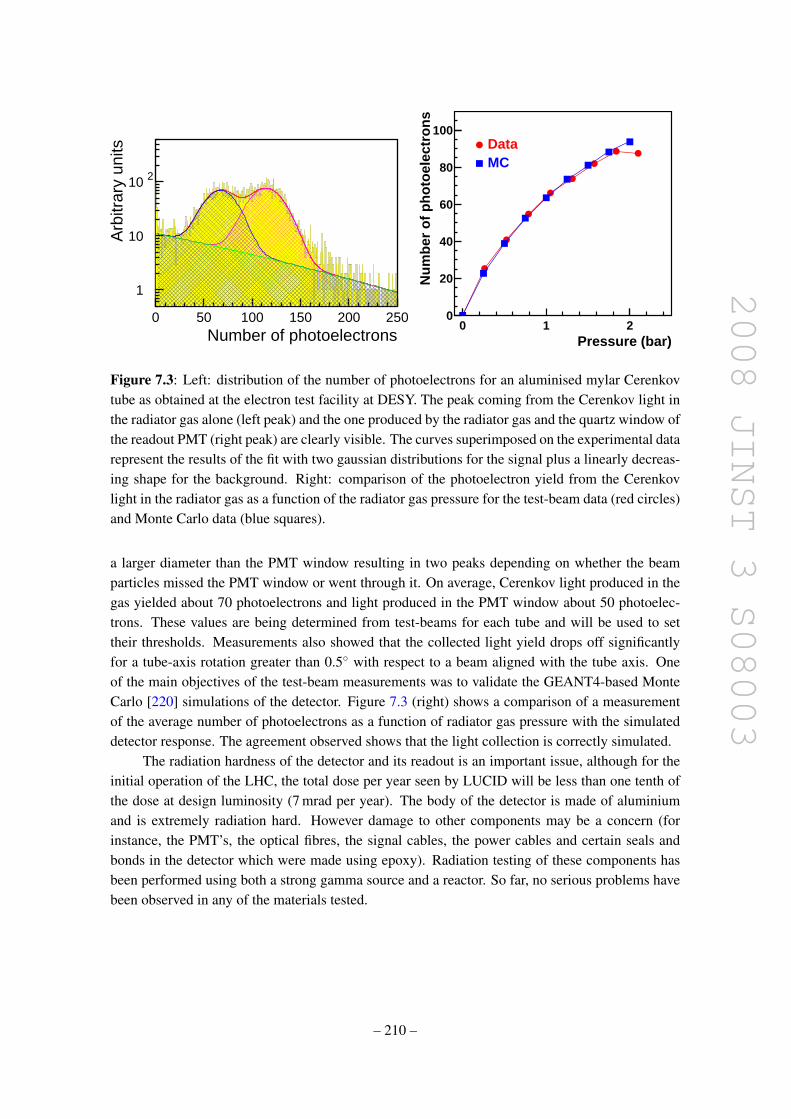
2008 JINST 3 S08003

1

10

10 2

0 50 100 150 200 250Number of photoelectrons

Arb

itrar

y un

its

0

20

40

60

80

100

0 1 2

DataMC

Pressure (bar)

Nu

mb

er o

f p

ho

toel

ectr

on

s

Figure 7.3: Left: distribution of the number of photoelectrons for an aluminised mylar Cerenkovtube as obtained at the electron test facility at DESY. The peak coming from the Cerenkov light inthe radiator gas alone (left peak) and the one produced by the radiator gas and the quartz window ofthe readout PMT (right peak) are clearly visible. The curves superimposed on the experimental datarepresent the results of the fit with two gaussian distributions for the signal plus a linearly decreas-ing shape for the background. Right: comparison of the photoelectron yield from the Cerenkovlight in the radiator gas as a function of the radiator gas pressure for the test-beam data (red circles)and Monte Carlo data (blue squares).

a larger diameter than the PMT window resulting in two peaks depending on whether the beamparticles missed the PMT window or went through it. On average, Cerenkov light produced in thegas yielded about 70 photoelectrons and light produced in the PMT window about 50 photoelec-trons. These values are being determined from test-beams for each tube and will be used to settheir thresholds. Measurements also showed that the collected light yield drops off significantlyfor a tube-axis rotation greater than 0.5 with respect to a beam aligned with the tube axis. Oneof the main objectives of the test-beam measurements was to validate the GEANT4-based MonteCarlo [220] simulations of the detector. Figure 7.3 (right) shows a comparison of a measurementof the average number of photoelectrons as a function of radiator gas pressure with the simulateddetector response. The agreement observed shows that the light collection is correctly simulated.

The radiation hardness of the detector and its readout is an important issue, although for theinitial operation of the LHC, the total dose per year seen by LUCID will be less than one tenth ofthe dose at design luminosity (7 mrad per year). The body of the detector is made of aluminiumand is extremely radiation hard. However damage to other components may be a concern (forinstance, the PMT’s, the optical fibres, the signal cables, the power cables and certain seals andbonds in the detector which were made using epoxy). Radiation testing of these components hasbeen performed using both a strong gamma source and a reactor. So far, no serious problems havebeen observed in any of the materials tested.

– 210 –

2008 JINST 3 S08003

7.1.3 LUCID installation in ATLAS

The LUCID detector is fully assembled and mechanically tested for gas leaks and light tightness.The front-end and readout scheme has been validated in the beam test at DESY. The calibration us-ing LED light injected into each Cerenkov tube has been successfully tested in the fully assembleddetectors. The detector is ready to be installed together with the beam-pipe in 2008.

7.2 The ALFA detector

Traditionally, the absolute luminosity at hadron colliders has been determined via elastic scatteringat small angles. This is also the approach pursued by ATLAS with the ALFA (Absolute LuminosityFor ATLAS) [213] detector. The optical theorem connects the elastic-scattering amplitude in theforward direction to the total cross-section and can be used to extract luminosity. In addition, otherinteresting physics topics may be explored with such scattering data [221].

The extremely small scattering angles (3 µrad) needed to make these measurements aresmaller than the nominal beam divergence. These measurements can therefore only be performedwith specially prepared beam conditions, which are also used for calibration of the LUCID detec-tor. High-beta (β ∗) optics in combination with reduced beam emittance are required. Moreoverthe detectors have to be placed far away from the interaction point and as close as possible to thebeam. The Roman-pot technique has been successfully used in the past [222] for measurementsvery close to circulating beams and has therefore been adopted for ATLAS. The Roman-pot con-cept is based upon a detector volume (the pot) that is separated from the vacuum of the acceleratorby a thin window but is connected with bellows to the beam-pipe and thus can be moved close tothe beam. The ATLAS Roman pots have been designed to move the detectors as close as 1 mm tothe beam, but only from above and below, due to the mechanical constraints imposed by the twohorizontal beam-pipes of the LHC, as shown in figure 7.4. The Roman pots will be located±240 maway from the interaction point, and on each side there will be two Roman-pot stations separatedby four metres.

The main requirements on the detectors which will be housed in the Roman pots are: aspatial resolution of about 30 µm, no significant inactive edge region, minimal sensitivity to theradio-frequency noise from the LHC beams and compatibility with the vacuum in the Roman pots.

Given these requirements, ATLAS has chosen a scintillating-fibre tracker. The high-β ∗ op-eration of the LHC corresponds to a very low instantaneous luminosity, and for this reason noradiation-hard technology is required for this specific set of detectors. Prototypes of the ALFAdetectors have been validated in beam tests at DESY [223] and CERN [224]. In order to fulfil thespatial resolution requirements, the detector is built of ten double-sided modules, each with 64 fi-bres arranged in stereo u− v geometry on both sides. The square fibres have a width of 0.5 mm.The effective area of the detector is somewhat smaller than the 32 × 32 mm2 due to the way thefibres are cut close to the beam (see figure 7.5). The modules are staggered in depth by multiplesof a tenth of the effective fibre pitch, i.e. 70 µm. The fibres are aligned and glued on a preciselymachined support structure made of titanium. Before assembly, the fibres are aluminised to reducelight losses and optical cross-talk. The fibre positions are measured by means of optical metrology

– 211 –

2008 JINST 3 S08003

Figure 7.4: Schematic view of the support mechanics for one of the ALFA detectors and of its lo-cation at a distance of 240 m from the ATLAS interaction point (left). One of the as-built structures,which will house the scintillating-fibre trackers (right).

at various stages of the manufacturing, resulting in a set of equations describing the location ofeach fibre in a given detector.

The overall layout with the front-end electronics is shown in figure 7.5. The module supportstructure is connected to a base-plate, which is mounted on the Roman-pot flange. The base-plates also house optical feed-through connectors coupling the fibres to the pixels of multi-anodephototubes. The multi-anode phototubes with 64 channels are aligned to the fibres and shieldedagainst residual stray magnetic fields. Anode signals from these phototubes are fed into the front-end boards and further processed by the front-end multi-anode readout chips.

To achieve an accurate alignment of the fibre tracker with respect to the centre of the beam,the Roman pots are equipped with special interleaved extrusions, yielding a vertical overlap areawhen in beam position. These extrusions are instrumented with three layers of vertically staggeredoverlap detectors consisting of 30 horizontally oriented fibres in each layer. The overlap detectorsuse the same type of fibres and are read out in the same way as the other detectors.

The central area is further instrumented with two optically separated trigger scintillator tilesproviding a fast L1 trigger signal. Single trigger tiles are used in each of the overlap extrusions. Thetrigger tiles are coupled to clear light-guide fibres routed to standard PMT’s with 8 mm diameter.The PMT signals are amplified and processed before being sent to the central trigger processor (seesection 8.2.3).

– 212 –

2008 JINST 3 S08003

Upper and lower

Roman pots

Front-end boards

Multi-anode

photomultiplier

Fibre connectors

10 x u-v fibres

Beam axis

Figure 7.5: Schematic layout of the ALFA detector in the Roman pot, showing the scintillating-fibre stack, the fibre connectors, the multi-anode photomultipliers, and the front-end boards. TheRoman pots (labelled as upper and lower) approach the beam-line from above and below (left).Details of the scintillating-fibre stack (right).

7.2.1 Experimental results from test-beam

Two test-beam campaigns were carried out for the ALFA detectors; the first one at DESY [223]to validate the detector design, and the second one at CERN [224] to test the overlap, trigger,and electronics concepts. Prototypes with ten modules but only a fraction of nominal fibres permodule were built and exposed to the beam. The test-beam facilities were partly equipped withhigh-precision silicon-strip detectors for precise resolution studies. The photoelectric yield of thescintillating fibres was extracted from charge-amplitude measurements of the multi-anode photo-tubes. The charge response of the multi-anode phototube to single photons was calibrated using apulsed blue LED. The average number of photoelectrons was 4.2± 0.5, with a relative cross-talkcontribution from adjacent fibres of about 3%.

The spatial detector resolution, obtained after deconvolution of the intrinsic contribution ofthe silicon reference detector of 30 µm, was determined to be 36 µm in both the x and y directions.For the low-energy electron beam used at DESY, a sizable resolution degradation is expected frommultiple scattering, as shown in an energy scan in figure 7.6. Using a high-energy hadron beamat CERN, where multiple scattering is irrelevant, a spatial resolution for ALFA of 25±3 µm wasdetermined, in agreement with GEANT4 [220] Monte-Carlo expectations.

– 213 –

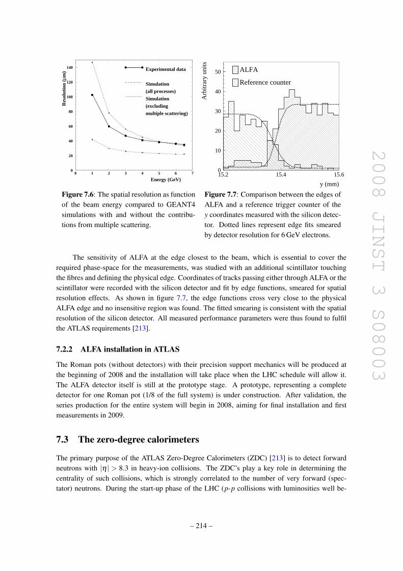
2008 JINST 3 S08003

0

20

40

60

80

100

120

140

0 1 2 3 4 5 6 7

Energy (GeV)

Res

olut

ion

(µm

) Experimental data

Simulation

(all processes)

Simulation

(excluding

multiple scattering)

0

10

20

30

40

50

15.2 15.4 15.6

ALFA

Reference counter

y (mm)

Arb

itrar

y un

itsFigure 7.6: The spatial resolution as functionof the beam energy compared to GEANT4simulations with and without the contribu-tions from multiple scattering.

Figure 7.7: Comparison between the edges ofALFA and a reference trigger counter of they coordinates measured with the silicon detec-tor. Dotted lines represent edge fits smearedby detector resolution for 6 GeV electrons.

The sensitivity of ALFA at the edge closest to the beam, which is essential to cover therequired phase-space for the measurements, was studied with an additional scintillator touchingthe fibres and defining the physical edge. Coordinates of tracks passing either through ALFA or thescintillator were recorded with the silicon detector and fit by edge functions, smeared for spatialresolution effects. As shown in figure 7.7, the edge functions cross very close to the physicalALFA edge and no insensitive region was found. The fitted smearing is consistent with the spatialresolution of the silicon detector. All measured performance parameters were thus found to fulfilthe ATLAS requirements [213].

7.2.2 ALFA installation in ATLAS

The Roman pots (without detectors) with their precision support mechanics will be produced atthe beginning of 2008 and the installation will take place when the LHC schedule will allow it.The ALFA detector itself is still at the prototype stage. A prototype, representing a completedetector for one Roman pot (1/8 of the full system) is under construction. After validation, theseries production for the entire system will begin in 2008, aiming for final installation and firstmeasurements in 2009.

7.3 The zero-degree calorimeters

The primary purpose of the ATLAS Zero-Degree Calorimeters (ZDC) [213] is to detect forwardneutrons with |η | > 8.3 in heavy-ion collisions. The ZDC’s play a key role in determining thecentrality of such collisions, which is strongly correlated to the number of very forward (spec-tator) neutrons. During the start-up phase of the LHC (p-p collisions with luminosities well be-

– 214 –

2008 JINST 3 S08003

low 1033 cm−2 s−1), the ZDC’s will enhance the acceptance of ATLAS central and forward detec-tors for diffractive processes and provide an additional minimum-bias trigger for ATLAS.

Significant backgrounds in hadron-collider experiments are created by beam-gas and beam-halo effects. These can be greatly reduced by requiring a tight coincidence from the two armsof the ZDC’s, located symmetrically with respect to the interaction point. For p-p scattering, thiscoincidence, as determined from PYTHIA [225] simulations, is found to be 9% of the total inelasticrate and will therefore be important for initial beam tuning at the beginning of LHC operation. Thetime resolution of the ZDC’s is roughly 100 ps, which is sufficient to locate the interaction point toabout 3 cm in z (along the beam axis). This would therefore provide some knowledge of the vertexlocation without using the inner detector information.

The ZDC’s reside in a slot in the TAN (Target Absorber Neutral) absorber, which wouldotherwise contain inert copper bars as shielding. The TAN is located at±140 m from the interactionpoint, at the place where the straight-section of the beam-pipe is divided back into two independentbeam-pipes.

7.3.1 ZDC module description

There will be four ZDC modules installed per arm: one electromagnetic (EM) module (about 29radiation lengths, X0, deep) and 3 hadronic modules (each about 1.14 interaction lengths, λ , deep).

Table 7.1 summarises the mechanical properties of the ZDC system. The EM module of onearm is shown in figure 7.8a). It consists of 11 tungsten plates, with their faces perpendicular to thebeam direction. The height of these plates is extended in the vertical direction with 290 mm longsteel plates. A total of 96 quartz rods of 1.0 mm diameter penetrate the tungsten plates parallel to thebeam in a 8×12 matrix, which is transverse to the beam. Along the face of the module the rods arebent upwards at an angle of 90 and are viewed by multi-anode phototubes capturing the Cerenkovlight from shower products of incident particles. The position of the rods containing a signal thuscorresponds to the position of the incident particle transverse to the beam, and the intensity of thelight reflects the energy of the particle. Only one of the arms, at −140 m, is equipped with theposition-sensing capability for its EM module.

Between the tungsten and steel plates are placed 1.5 mm quartz strips which are routed ver-tically and are viewed from above by photomultiplier tubes via air light-guides. These strips areactually rows of quartz rods called strips, in order to distinguish them from the position-measuringrods. These strips are depicted in figure 7.8b). The purpose of the strips is to obtain a second,improved measurement of the incident particle energy. In the position-sensing EM module thereare four such light-guides, side by side, since more than one incident particle per event is expected.

The hadronic modules are similar, but while the EM module maps the 96 position-measuringrods each onto one pixel of the multi-anode phototube, the hadronic modules map clusters of fourrods into individual phototubes and have only one light-guide. Not all hadronic modules haveposition-sensing rods (there is only one position-sensing module per arm).

– 215 –

2008 JINST 3 S08003

a) b)

Photomultipliers

Multi-anodephotomultipliers

Rod holder

Light guide

Steel

Straightquartz rods

Tungsten

Bentquartz rods

Quartz strips

Side view Top view Rear view

Beam

Beam

Figure 7.8: a) The electromagnetic ZDC module. The incident particles impinge on tungstenplates at the bottom of the module and produces showers of particles. The quartz rods pick upthe Cerenkov light generated by the shower and transmit it to multi-anode phototubes at the top ofthe module. The phototubes measure light from the quartz strips through four air light-guides. b)Details showing the placement of the quartz strips.

7.3.2 Calibration and monitoring

7.3.2.1 Flashers

Measurements over long periods of time and limited access to the tunnel require that the PMTgains be remotely monitored to an accuracy of about 1%. This can be achieved with a systembased on blue LED’s. A controllable generator located in the underground side-cavern USA15 willexcite the LED in the tunnel. Each PMT will view a fibre connected to the LED, and one fibre willilluminate each large single channel PMT.

The LED is mounted opposite a pin-diode which tracks its stability. Around the pin-diodeare eight primary optical fibres. Light in these fibres will travel 5 m to the modules. The light fromthree of these primary fibres is split further into eight secondary fibres. Light from each of thesesecondary fibres impinges on each of the 24 phototubes in the hadronic position-sensing module.Four more of the eight primary fibres will calibrate the phototubes in the hadronic position-sensingand energy-measuring modules. The eighth primary fibre is a spare.

The LED monitoring system is not subjected to the large doses of radiation seen in the ZDC’sand so deterioration of the system due to radiation damage is not expected.

– 216 –

2008 JINST 3 S08003

Table 7.1: Summary of ZDC mechanical properties.

Electromagnetic Electromagnetic Hadronic(at −140 m) (at +140 m) (per arm)

Number of modules 1 1 3Number of position-sensing modules 1 none 1Number of energy-measuring 4 1 3light-guidesTotal depth 29 X0 29 X0 4.6 λ (includes

EM module)Module size (mm): width 93.8 93.8 93.8

height 738 738 738depth 150 150 150

Number of plates/module 11 11 11Tungsten plate size (mm): width 91.4 91.4 91.4

height 180 180 180depth 10 10 10

Module weight (kg) 80 80 80Number of 1.5 mm quartz strips 648 648 648Number of 1 mm pixel rods 96 none 96Number of pixel readout channels 96 none 24

7.3.2.2 Particles

Full calibration of the ZDC detector begins with the determination of the gains in all rod/phototubechains, and continues with the measurement of shower-shape distribution functions, such as thedependence of single-rod amplitudes on the distance to the shower centre. These parameters willbe permanently monitored during operation. This preliminary calibration is followed by one usingπ0 decays in situ in p-p collisions. During heavy-ion operations, peripheral ion collisions willyield samples of mono-energetic neutrons with the beam energy of 2.75 TeV, providing a usefulredundancy check of the calibration constants.

7.3.3 ZDC installation in ATLAS

The ZDC is being installed in two stages because it shares the TAN location with the LHCf de-tector [226]. The LHCf experiment will run during early 43-bunch operation of the LHC and willthen be removed. Since the LHCf detector occupies the space of the first ZDC module in eacharm, only the three downstream modules in each arm will be installed during this phase. The fullZDC will be in place for the luminosity ramp-up of the machine beyond 2008. As soon as the LHCreaches luminosities above 1033 cm−2 s−1, the ZDC modules will be removed for p-p operationand reinstalled only for the heavy-ion periods. This will be necessary in order to minimise radiationdamage to the quartz radiator in the ZDC.

– 217 –

2008 JINST 3 S08003

Chapter 8

Trigger, data acquisition, and controls

8.1 Introduction to event selection and data acquisition

As described in chapter 1, the trigger consists of three levels of event selection: Level-1 (L1),Level-2 (L2), and event filter. The L2 and event filter together form the High-Level Trigger (HLT).The L1 trigger is implemented using custom-made electronics, while the HLT is almost entirelybased on commercially available computers and networking hardware. A block diagram of thetrigger and data acquisition systems is shown in figure 8.1.

The L1 trigger searches for signatures from high-pT muons, electrons/photons, jets, and τ-leptons decaying into hadrons. It also selects events with large missing transverse energy (Emiss

T )and large total transverse energy. The L1 trigger uses reduced-granularity information from asubset of detectors: the Resistive Plate Chambers (RPC) and Thin-Gap Chambers (TGC) for high-pT muons, and all the calorimeter sub-systems for electromagnetic clusters, jets, τ-leptons, Emiss

T ,and large total transverse energy. The maximum L1 accept rate which the detector readout systemscan handle is 75 kHz (upgradeable to 100 kHz), and the L1 decision must reach the front-endelectronics within 2.5 µs after the bunch-crossing with which it is associated.

The L2 trigger is seeded by Regions-of-Interest (RoI’s). These are regions of the detec-tor where the L1 trigger has identified possible trigger objects within the event. The L2 triggeruses RoI information on coordinates, energy, and type of signatures to limit the amount of datawhich must be transferred from the detector readout. The L2 trigger reduces the event rate tobelow 3.5 kHz, with an average event processing time of approximately 40 ms.

The event filter uses offline analysis procedures on fully-built events to further select eventsdown to a rate which can be recorded for subsequent offline analysis. It reduces the event rate toapproximately 200 Hz, with an average event processing time of order four seconds.

The HLT algorithms use the full granularity and precision of calorimeter and muon chamberdata, as well as the data from the inner detector, to refine the trigger selections. Better informationon energy deposition improves the threshold cuts, while track reconstruction in the inner detectorsignificantly enhances the particle identification (for example distinguishing between electrons andphotons). The event selection at both L1 and L2 primarily uses inclusive criteria, for example high-ET objects above defined thresholds. One exception is the L2 selection of events containing thedecay of a B-hadron, which requires the reconstruction of exclusive decays into particles with lowmomentum.

– 218 –

2008 JINST 3 S08003

Figure 8.1: Block diagram of the ATLAS trigger and data acquisition systems (see sections 8.2and 8.3 for further details).

The data acquisition system (DAQ) receives and buffers the event data from the detector-specific readout electronics at the L1 trigger rate. The data transmission is performed over point-to-point Readout Links (ROL’s). It transmits to the L2 trigger any data requested by the trigger(typically the data corresponding to RoI’s) and, for those events fulfilling the L2 selection criteria,event-building is performed. The assembled events are then moved by the data acquisition systemto the event filter, and the events selected there are moved to permanent event storage.

In addition to controlling movement of data down the trigger selection chain, the data acqui-sition system also provides for the configuration, control and monitoring of the ATLAS detectorduring data-taking. Supervision of the detector hardware (gas systems, power-supply voltages,etc.) is provided by the Detector Control System (DCS).

Section 8.2 presents the design, algorithms, and implementation of the L1 trigger. The HLTand data acquisition system are described in section 8.3, which gives an overview of the flow ofevents through the system, a brief description of the main system components, and the performanceexpected for initial operations. The implementation and capabilities of the DAQ/HLT are presentedin section 8.4. Finally, the detector control system is described in section 8.5.

– 219 –

2008 JINST 3 S08003

Calorimeter triggers

missEMJet

ET

ET

µ

Muon trigger

Detector front-ends L2 trigger

Central trigger

processor

Timing, trigger and

control distribution

Calorimeters Muon detectors

DAQ

L1 trigger

Regions-

of-Interest

Figure 8.2: Block diagram of the L1 trigger. The overall L1 accept decision is made by the centraltrigger processor, taking input from calorimeter and muon trigger results. The paths to the detectorfront-ends, L2 trigger, and data acquisition system are shown from left to right in red, blue andblack, respectively.

8.2 The L1 trigger

The flow of the L1 trigger is shown in figure 8.2. It performs the initial event selection based oninformation from the calorimeters and muon detectors. The calorimeter selection is based on in-formation from all the calorimeters (electromagnetic and hadronic; barrel, end-cap and forward).The L1 Calorimeter Trigger (L1Calo) aims to identify high-ET objects such as electrons and pho-tons, jets, and τ-leptons decaying into hadrons, as well as events with large Emiss

T and large totaltransverse energy. A trigger on the scalar sum of jet transverse energies is also available. Forthe electron/photon and τ triggers, isolation can be required. Isolation implies that the energeticparticle must have a minimum angular separation from any significant energy deposit in the sametrigger. The information for each bunch-crossing used in the L1 trigger decision is the multiplicityof hits for 4 to 16 programmable ET thresholds per object type.

The L1 muon trigger is based on signals in the muon trigger chambers: RPC’s in the barreland TGC’s in the end-caps. The trigger searches for patterns of hits consistent with high-pT muonsoriginating from the interaction region. The logic provides six independently-programmablepT thresholds. The information for each bunch-crossing used in the L1 trigger decision is themultiplicity of muons for each of the pT thresholds. Muons are not double-counted across thedifferent thresholds.

– 220 –

2008 JINST 3 S08003

The overall L1 accept decision is made by the Central Trigger Processor (CTP), which com-bines the information for different object types. Trigger menus can be programmed with up to 256distinct items, each item being a combination of requirements on the input data. The trigger deci-sion, together with the 40.08 MHz clock and other signals, is distributed to the detector front-endand readout systems via the Timing, Trigger and Control (TTC) system, using an optical-broadcastnetwork.

While the L1 trigger decision is based only on the multiplicity of trigger objects (or flagsindicating which thresholds were passed, for global quantities), information about the geometriclocation of trigger objects is retained in the muon and calorimeter trigger processors. Upon theevent being accepted by the L1 trigger, this information is sent as RoI’s to the L2 trigger (seesection 8.3.6), where it is used to seed the selection performed by the HLT.

An essential function of the L1 trigger is unambiguous identification of the bunch-crossing ofinterest. The very short (25 ns) bunch-crossing interval makes this a challenging task. In the caseof the muon trigger, the physical size of the muon spectrometer implies times-of-flight exceedingthe bunch-crossing interval. For the calorimeter trigger, a serious complication is that the width ofthe calorimeter signals extends over many (typically four) bunch-crossings.

While the trigger decision is being formed, the information for all detector channels has to beretained in pipeline memories. These memories are contained in custom electronics placed on ornear the detector, where often radiation levels are high and access is difficult. In the interest of costand reliability, it is desirable to keep the pipeline length as short as possible. The L1 latency, whichis the time from the proton-proton collision until the L1 trigger decision, must therefore be kept asshort as possible. The design of the trigger and front-end systems requires the L1 latency to be lessthan 2.5 µs, with a target latency of 2.0 µs, leaving 0.5 µs contingency. About 1 µs of this timeis accounted for by cable-propagation delays alone. To achieve this aim, the L1 trigger is imple-mented as a system of purpose-built hardware processors, which are described in more detail below.

8.2.1 Calorimeter trigger

L1Calo [227] is a pipelined digital system designed to work with about 7000 analogue triggertowers of reduced granularity (0.1× 0.1 in ∆η ×∆φ in most parts, but larger at higher |η |) fromthe electromagnetic and hadronic calorimeters. It sends the results for each LHC bunch-crossingto the CTP approximately 1.5 µs after the event occurs, resulting in a total latency for the L1Calochain of about 2.1 µs, well within the allowed envelope.

The L1Calo system is located off-detector in the service cavern USA15. Its architecture,shown in figure 8.3, consists of three main sub-systems. The pre-processor digitises the analogueinput signals, then uses a digital filter to associate them with specific bunch-crossings. It uses alook-up table to produce the transverse-energy values used for the trigger algorithms. The dataare then transmitted to both the Cluster Processor (CP) and Jet/Energy-sum Processor (JEP) sub-systems in parallel. The CP sub-system identifies electron/photon and τ-lepton candidates with ET

above the corresponding programmable threshold and satisfying, if required, certain isolation cri-teria. The JEP receives jet trigger elements, which are 0.2×0.2 sums in ∆η×∆φ , and uses theseto identify jets and to produce global sums of scalar and missing transverse energy. Both proces-sors count the multiplicities of the different types of trigger objects. The CP and JEP send these

– 221 –

2008 JINST 3 S08003

LAr(EM)

Tile/LAr(hadronic)

ET,ET

ET sum

Ex, Ey

ETsums

Local maximum

Jets

Counting

Jet-finding

RoI's

Bunch-crossing ident.

Look-up table

BC-mux

~7000 analogue links

L1 central trigger processor

L1 muontrigger

Ondetector

InUSA15

Local maximum

Cluster processor

PPM's

9-bit jet elements

Serial links(400 Mbit/s)

8-bit trigger towers

JEM's CPM's

Cluster-finding

Jet/energy processor

To ROD's(for L2)

RoI's

(e / and h

e / h

To ROD's (for DAQ)

ToROD's

To ROD's (for DAQ)

2x2 sum

Twisted pairs, <70 m

Pre-processor10-bit FADC

Calorimeters

Analogue Sum

Receiver

CountingCMM's

EM+hadronic 2x2 sums

DAQ) (for

miss

Figure 8.3: Architecture of the L1 calorimeter trigger. Analogue data from the calorimeters aredigitised and associated with the correct bunch-crossing in the pre-processor and then sent to twoalgorithmic processors, the jet/energy-sum processor and the cluster processor. The resulting hitcounts and energy sums are sent to the central trigger processor.

feature multiplicities, as well as transverse-energy threshold information, to the CTP for everybunch-crossing.

When there is a L1 Accept (L1A) decision from the CTP, the stored data from the L1Calo sub-systems are read out to the data acquisition system: this includes input data, intermediate calcula-tions and trigger results in order to allow full monitoring and verification of the L1 trigger func-tionality. These data can also provide useful diagnostics for the LHC machine (see section 9.10)and the ATLAS sub-detectors. The types and positions of jet, τ-lepton and electromagnetic clustercandidates are also collected and sent to the RoI builder (see section 8.3.6) for use by the L2 trigger.

The L1Calo architecture is relatively compact, with a minimal number of crates and cablelinks. This helps in reducing the latency. Some of the hardware modules were designed to fulfilseveral different roles in the system, in order to reduce hardware costs and design efforts, as wellas to reduce the number of spares required.

– 222 –

2008 JINST 3 S08003

8.2.1.1 The analogue front-end

Analogue signals from trigger towers in all the calorimeters are sent to the USA15 cavern on 16-way twisted-pair cables. These cables are specially routed to minimise their length, and hencethe trigger latency; they range from about 30 m to 70 m in length. Liquid-argon electromagneticcalorimeter signals are converted from energy to transverse energy in the tower builder boardslocated on the detector, but all hadronic calorimeter signals are transmitted proportional to energy.All the trigger-tower signals arrive at 64-channel receiver modules. The main function of thereceiver modules is to adjust the gains, in order to provide transverse energy rather than energy forhadronic calorimeter signals, and to compensate for differences in energy calibration and signalattenuation in the long cables. The receivers reshape the signals, and contain linear, variable-gain amplifiers controlled by DAC’s. Receiver outputs are sent as differential signals on shorttwisted-pair cables to the pre-processor. A further function of the receivers is to monitor a small,programmable selection of analogue input signals.

8.2.1.2 The pre-processor

The pre-processor consists of eight 9U VMEbus crates. Four crates process electromagnetic triggertowers and four process hadronic towers. Each crate contains 16 Pre-Processor Modules (PPM’s)which each receive four analogue cables on the front panel and process 64 analogue input signals.The granularity of these signals is reduced compared to the full calorimeter data. This is done byanalogue summing at the detector of variable numbers of calorimeter cells, ranging from a few upto 60. The main signal processing is performed by 16 multi-chip modules, each of which processesfour trigger towers. Ten-bit Flash ADC’s (FADC’s) digitise the signals with a sampling frequencyof 40.08 MHz. Fine adjustment of the timing of each digitisation strobe is performed by a four-channel ASIC, which provides programmable delays in steps of 1 ns across the 25 ns LHC clockperiod. The digitised values are then sent to a custom pre-processor ASIC.

The pre-processor ASIC synchronises the timing of the four inputs, to compensate for dif-ferent times-of-flight and signal path-lengths. It then assigns signals to the correct bunch-crossing,as detailed below. A look-up table is used to carry out pedestal subtraction, apply a noise thresh-old, and do a final transverse-energy calibration, resulting in 8-bit trigger-tower energies. Finally,it performs bunch-crossing multiplexing (see below) for the CP and it sums the four values into0.2× 0.2 jet elements (2× 2 sum) for the JEP. Two 10-bit low-voltage differential signalling(LVDS) serialisers operating at 400 Mbit/s transmit the processed trigger-tower data to the CP,while a third serialiser sends the summed 9-bit jet elements to the JEP.

The pre-processor ASIC reads out data to the data acquisition system upon receiving a L1Asignal. The readout data are taken from pipeline memories at two stages: the raw digitised valuesfrom the FADC’s, and the 8-bit processed trigger-tower data from the look-up tables. Data fromthe bunch-crossing of interest, as well as a programmable number of bunch-crossings around it(typically up to five in all), allow monitoring of pulse shapes at the FADC’s, and of the bunch-crossing identification and energy calibration at the look-up table outputs. These readout data areserialised and sent to the data acquisition readout over an optical fibre. In addition, various ratesbased on the input signals are monitored and histogrammed automatically in the ASIC and are readout by VMEbus.

– 223 –

2008 JINST 3 S08003

Bunch-crossing identification. The analogue pulses from the electromagnetic and hadroniccalorimeters have widths of several bunch-crossings, so it is essential that trigger-tower signalsare associated with the correct bunch-crossing. This is a crucial requirement not only for normal-size pulses, but also for saturated pulses (above about 250 GeV) and for pulses as small as possible(down to 2–3 GeV, just above the noise level). The pre-processor ASIC is capable of identify-ing a signal’s bunch-crossing using three different methods, which provides ample redundancy forconsistency checks during commissioning.

For normal, unsaturated signals, a digital pipelined finite-impulse-response filter processesfive consecutive FADC samples. A subsequent peak-finder attributes the maximum value of thissum to the corresponding bunch-crossing. The working range of the method spans from smalltrigger signals (energy depositions of a few GeV) up to the near-saturation level of around 250 GeV.

For saturated signals, two consecutive samples are compared to a low and a high threshold,making use of the finite peaking-time (approximately 50 ns) of an analogue input signal. Thus,detection of a leading edge allows attribution of the virtual peak to a specific bunch-crossing. Thismethod is valid from around 200 GeV up to the maximum energy range of the calorimeters.

A third method uses comparators with programmable thresholds on the analogue input sig-nals to present a rising-edge signal to the multi-chip modules. Given the known peaking time,bunch-crossing identification can be performed using an appropriate programmed delay in the pre-processor ASIC. The validity of this method begins well above the comparator threshold and ex-tends up to the full energy range. There is thus a large overlap with the two previous methods,allowing consistency checks between the methods to be performed.

The finite-impulse-response filter output is presented to the look-up table to extract a cali-brated ET value for the trigger tower. If the bunch-crossing identification criteria are met, this valueis sent to the CP outputs. In the case of saturation, the tower is assigned the maximum 8-bit valueof 255 GeV. For the JEP outputs, any 0.2×0.2-sum jet element which contains a saturated triggertower, or which has a 9-bit sum in overflow, is assigned the maximum 9-bit value of 512 GeV. Atower or jet element with a maximum value is understood to be saturated by the CP and/or JEPsub-systems. The trigger menu will be set up so that any event where a saturation condition occurswill produce a L1A signal, and the RoI’s sent to the L2 trigger will be flagged by saturation bits.

Bunch-crossing multiplexing. The data from the pre-processor modules consist of four 8-bittrigger towers per multi-chip module to the CP, and one 9-bit 0.2×0.2-sum jet element to the JEP.To economise on the number of links needed, it was noted that the bunch-crossing identificationalgorithm is essentially a peak-finding scheme. This means that an occupied bunch-crossing willalways be followed by an empty (zero) one. This allows two trigger towers being sent to the CP toshare a single serial link. Trigger towers are paired at the pre-processor ASIC output stage, and thescheme is called Bunch-Crossing Multiplexing (BC-mux). By using it, data transmission to the CPsub-system is achieved with only two links per multi-chip module instead of four. However, for theJEP, where a sum of four towers is transmitted, this cannot be done.

Output signal fan-out and pre-compensation. The high-speed serial outputs to the CP and JEPare fanned out in order to provide the trigger algorithms with overlapping data between detectorquadrants in azimuth. The data pass through the back-plane to 11 m long shielded parallel-pair

– 224 –

2008 JINST 3 S08003

cables. RC pre-compensation is done to improve signal-driving capabilities, since observed signalattenuation and distortion from the cables may compromise data integrity. Bit-error rates of lessthan 10−14 have been achieved.

8.2.1.3 The cluster and jet/energy-sum processors

The CP and JEP sub-systems share many architectural features and some common hardware. Thejet algorithm in the JEP and the electron/photon and τ cluster algorithms in the CP both performfeature searches in overlapping, sliding windows. Therefore, a large amount of data duplicationbetween processor modules is required, and this is done as follows. Both sub-systems divide thecalorimeters into four azimuthal quadrants, with each processor module within a quadrant cover-ing a slice in pseudorapidity and 90 in azimuth. Overlapping data from neighbouring azimuthalquadrants are provided by duplicated serial links from the pre-processor. Within each quadrant,modules only need to share input data with their nearest neighbours, over short (roughly 2 cm)point-to-point back-plane links. This architecture minimises the number of cable links from thepre-processor, and the back-plane fan-out is simplified.

The CP is a four-crate system, with 14 Cluster Processor Modules (CPM’s) in eachcrate covering one calorimeter quadrant. The JEP is contained in two crates, each containingeight Jet/Energy Modules (JEM’s) from two opposing quadrants in azimuth (16 JEM’s total). Re-sults from the processor modules are brought to two Common Merger Modules (CMM’s) in eachcrate: these sum the data to produce crate-level results. The CMM’s also perform the system-levelsummation of data from the different crates, and transmit the final results to the CTP.

The electron/photon and τ triggers extend out to |η | = 2.5, which is the fiducial limit forprecision measurements with the inner detector and electromagnetic calorimetry. The jet trig-ger extends out to |η | = 3.2. The Emiss

T and total transverse-energy triggers include the forwardcalorimetry, in particular to provide adequate Emiss

T performance, which means that they extendto |η | = 4.9. This also allows the FCal to be used for forward-jet triggers.

8.2.1.4 The cluster processor module

The electron/photon trigger algorithm [228], shown in figure 8.4, identifies 2× 2 clusters of trig-ger towers in which at least one of the four possible two-tower sums (1× 2 or 2× 1) of nearest-neighbour electromagnetic towers exceeds a pre-defined threshold. Isolation-veto thresholds areset for the 12-tower surrounding ring in the electromagnetic calorimeter, as well as for the 2× 2hadronic-tower core sum behind the cluster and the 12-tower hadronic ring around it. All thesethresholds are programmable.

The τ algorithm uses the same basic elements to select narrow hadronic jets. Each of thefour possible two-tower sums of nearest-neighbour electromagnetic towers is added to the 2× 2hadronic-tower core sum directly behind, and the result is compared to a pre-defined threshold.Isolation veto thresholds are set separately for each of the surrounding 12-tower rings in both theelectromagnetic and hadronic calorimeters.

The isolation thresholds for both algorithms are absolute values, rather than ratios of isolationenergy to cluster energy. This simpler approach was chosen on the basis of studies, which showed

– 225 –

2008 JINST 3 S08003

Vertical sumsΣ

Σ Horizontal sums

Σ Σ

Σ

Σ

Electromagneticisolation ring

Hadronic inner coreand isolation ring

Electromagneticcalorimeter

Hadroniccalorimeter

Trigger towers (∆η × ∆φ= 0.1 × 0.1)

Local maximum/Region-of-interest

R

>

>

>

>

Figure 8.4: Electron/photon and τ triggeralgorithms, as described in the text.

Figure 8.5: ET local-maximum test for acluster/RoI candidate. The η-axis runs fromleft to right, and the φ -axis from bottom totop. The symbol R refers to the candidate2×2 region being tested.

that the expected isolation sums are relatively insensitive to shower energies. In practice, high-energy clusters will generally have looser isolation criteria to maximise the efficiency for possiblelow-rate exotic signal processes, while lower-energy clusters will have stricter isolation criteria inorder to minimise the rates at the expense of a limited loss of signal.

These algorithms are run over all possible 4× 4 windows, which means that the windowsoverlap and slide by steps of 0.1 in both η and φ . This implies that an electron/photon or τ

cluster can satisfy the algorithm in two or more neighbouring windows. Multiple-counting ofclusters is avoided by requiring the sum of the four central electromagnetic plus the sum of thefour central hadronic towers to be a local maximum with respect to its eight nearest overlappingneighbours. In order to avoid problems in comparing digital sums with identical values, four ofthe eight comparisons are ‘greater than’ while the other four are ‘greater than or equal to’, asshown in figure 8.5. The location of this 2×2 local maximum also defines the coordinates of theelectron/photon or τ RoI.

The CPM identifies and counts clusters satisfying sets of threshold and isolation criteria.Eight threshold sets are reserved for electron/photon triggers, while eight further threshold sets caneach be used for either electron/photon or τ triggers.

Each CPM receives and deserialises input data on 80 LVDS cables from the pre-processormodules, brought in to the rear of the module through back-plane connectors. The data are thenshared between neighbouring modules via the back-plane, and finally fanned out to eight CPFPGA’s, which perform the clustering algorithms. The serialiser FPGA’s also store the input datain pipelines for eventual readout to the data acquisition system upon reception of a L1A signal.

– 226 –

2008 JINST 3 S08003

The eight CP FPGA’s each service eight overlapping 4×4 windows. Pipelines implementedin each one of them save output data for readout to the data acquisition system, and also save clustertypes and coordinates for readout as RoI’s to the L2 trigger. Two hit-multiplicity FPGA’s collectand then sum the 3-bit cluster multiplicities from the CP FPGA’s, for reporting to the crate-levelmerging of CP results. These multiplicities are transmitted via the back-plane. If more than seveninstances of a cluster type are identified (a very rare occurrence, given that the mean occupancyis less than one), the multiplicity is reported as seven. Two additional FPGA’s collect input datafrom the serialiser FPGA’s, RoI data from the CP FPGA’s, and output data from the hit-multiplicityFPGA’s upon reception of a L1A signal, and transmit them to readout driver modules serving thedata acquisition system and the L2 trigger on two optical fibres from the front panel of the module.

8.2.1.5 The jet/energy module

The Jet/Energy Module (JEM) works with jet elements which are the sums of 2×2 trigger towersin the electromagnetic calorimeters added to 2× 2 trigger towers in the hadronic calorimeters.The jet algorithm identifies ET sums within overlapping windows consisting of 2× 2, 3× 3, or4× 4 jet elements, corresponding to window sizes of 0.4, 0.6, or 0.8 in η and φ , as shown infigure 8.6. These sums are then compared to pre-defined jet energy thresholds. Multiple-countingof jet candidates is avoided by requiring the window to surround 2×2 jet elements whose sum is alocal maximum, with the same definition as for electron/photon and τ clusters. The location of this2×2 local maximum also defines the coordinates of the jet RoI. Eight independent combinationsof jet ET threshold and window size are available for trigger menus.

The energy-summation algorithm produces sums of ET , Ex and Ey, and uses the system-levelsums of these to report on four total-ET and eight Emiss

T thresholds to the CTP.Each JEM receives and deserialises data from 88 LVDS links, corresponding to 44 jet el-

ements for both the electromagnetic and hadronic calorimeters. Four input FPGA’s receive thedata, sum the electromagnetic and hadronic parts of each jet element to 10-bit values, and sendthese sums to the main processor FPGA’s on the same and neighbouring modules. Pipelines ineach input FPGA save input data for readout to the data acquisition system upon reception of aL1A signal.

The jet and energy-summation algorithms are implemented in two large main-processorFPGA’s per JEM. The main processors are also responsible for reporting results to the crate-levelmerging, as well as pipelining of data acquisition and RoI information for readout. The jet outputof each JEM is a data stream consisting of eight 3-bit jet multiplicities. The energy output is alsoa data stream containing the values of Ex and Ey, each compressed from 12 bits to an 8-bit (6-bitmantissa plus two multiplier bits) quad-linear scale (a data-compression technique that multipliesthe mantissa by 1, 4, 16, or 64).

A single readout-controller FPGA collects input data from the input FPGA’s, and output andRoI data from the main processor FPGA’s, for readout to readout driver modules serving dataacquisition and the L2 trigger on two optical fibres from the front panel of the module.

– 227 –

2008 JINST 3 S08003

Window 0.6 x 0.6 Window 0.8 x 0.8Window 0.4 x 0.4

Figure 8.6: Jet trigger algorithms, based on 0.2×0.2 jet elements and showing RoI’s (shaded). Inthe 0.6×0.6 case there are four possible windows containing a given RoI. In the 0.8×0.8 case theRoI is required to be in the centre position, in order to avoid the possibility of two jets per window.

8.2.1.6 The common merger module

Two modules in each CP and JEP crate carry out crate-level merging of results received from thecrate’s processor modules. In the CP crates, each merger module is responsible for calculating3-bit cluster multiplicities for eight of the 16 electron/photon and τ cluster definitions. In theJEP crates, one merger module produces 3-bit multiplicities for the eight jet definitions, while theother produces sums of ET , Ex and Ey. Each Common Merger Module (CMM) receives data fromthe crate’s 14 CPM’s or 16 JEM’s, over point-to-point links on the crate back-plane.

The CMM carries out all of these merging functions by using different firmware versions.Each CMM receives up to 400 bits of data per bunch-crossing from the crate’s CPM’s or JEM’s.A large FPGA performs crate-level merging. Parallel LVDS cable links between the sub-systemcrates bring all crate-level results to one CMM of each type, which is designated as the system-merger CMM. A second FPGA on the CMM carries out the system-level merging.

At the system level, the CMM carries out the logic to provide global trigger results. Three-bitoverall multiplicities for each of the electron/photon, τ , and jet thresholds are formed and sent tothe CTP. The overall sums of Ex and Ey are applied together as the address to a look-up table. In oneoperation this works out whether the resulting vector sum, i.e. missing ET , is above or below eightprogrammable missing-ET thresholds and codes the result in an eight-bit word. For total scalar ET ,the global sum is compared to four threshold values. Finally, a rough approximation of the total ET

in jets, based on the numbers of jets passing each of the eight jet thresholds, is compared to fourthreshold values.

All of these calorimeter trigger results are passed to the CTP by cable. As with other pro-cessor modules, input and output data on each CMM are stored in FIFO’s and read out to the dataacquisition system over an optical fibre. RoI data on the missing and total ET values are sent to L2.

8.2.1.7 The processor back-plane

The CP and JEP use a common, custom processor back-plane. It has 16 CPM/JEM positionsflanked by two CMM positions. At the left it has a slot for a commercial VMEbus CPU. At the rightis a slot for a timing control module, which interfaces to the TTC (e.g. to distribute clock signals)

– 228 –

2008 JINST 3 S08003

and to the detector control system, which uses CANbus to monitor voltages and temperatures onall trigger modules.

The processor back-plane is a monolithic printed-circuit board of 9U height. It is popu-lated almost entirely with 2 mm hard-metric connectors, with 1148 signal and ground pins ineach JEM/CPM and CMM position. There are point-to-point links between neighbouring pro-cessor modules for input data fan-in/fan-out. Connections are provided from each CPM or JEM tothe two CMM’s at the right and left of the processor modules. To conserve pins, a non-standardVMEbus with the minimum possible number of pins (43 signals with 16 data bits and 24 addressbits) is used.

The LVDS serial-input and merger-interconnect cables are connected to the rear of the pro-cessor back-plane and passed through it to the modules in front. This results in a system with fewercables on the front panels of the modules and, as a consequence, hopefully fewer recabling errorsand less cable damage over the lifetime of the experiment.

8.2.1.8 The readout driver

The trigger system has two separate readout systems. Input, output, and some intermediate datafrom each module are read out to the data acquisition system and at the same time the CP and JEPsub-systems report feature types and coordinates as RoI data to the L2 trigger.

The readout system has been designed to handle one bunch-crossing of RoI data and up tofive bunch-crossings of data acquisition data per event at a L1A rate of up to 75 kHz. A commonapproach has been adopted in all L1Calo sub-systems for data acquisition and RoI readout.

On each module to be read out, readout FIFO’s on each processor FPGA or ASIC are readout as serial streams to a readout controller FPGA for timing alignment. This passes the serialstreams in parallel to the inputs of a G-link (high-speed serial link) transmitter, which transmitsthem serially at 800 Mbit/s over optical fibres to a Readout Driver (ROD).

A common ROD module is used by both the data acquisition and RoI readout sub-systems togather and report data from the pre-processor modules, CPM’s, JEM’s, and CMM’s, using differentfirmware configurations for different readout tasks and modules. The ROD is a 9U-module residingin a standard VME64x crate. It has 18 G-link receivers, which pass their parallel outputs to theFPGA’s for data compression, zero suppression, and some data monitoring. The ROD also containsfour S-link transmitters on a rear-transition module for passing compressed event data to the dataacquisition and RoI readout buffers. The S-link interface specification defines the signals andprotocol for the readout links; it does not define the hardware implementation. Routing of data tothe different outputs is carried out by a switch controller FPGA, whose settings depend on the typeand source of data being read out. In addition, a further large FPGA provides monitoring capabilityon a sample of readout data.

8.2.2 Muon trigger

The L1 muon trigger is based on dedicated finely segmented detectors (the RPC’s in the barrel andthe TGC’s in the end-caps, as described in detail in section 6.6) with a sufficient timing accuracyto provide unambiguous identification of the bunch-crossing containing the muon candidate.

– 229 –

2008 JINST 3 S08003

Low-pT

5 10 15 m0

RPC3

RPC2 (pivot)

RPC1

High-pT

MDT

MDT

MDT

MD

T

MD

T

Pad

RoI

Barrel large

sector

Barrel small

sector∆η=0.1

∆η=0.2

η=0

Trigger large sector

Trigger large sector

Trigger small sector

Trigger small sector

∆φ

=0

.1∆

φ=

0.2 -CMη

φ−C

M

∆η=0.2

∆φ=0.1

∆η=0.1

∆φ

=0.2

Figure 8.7: Schema (left) and segmentation (right) of the L1 muon barrel trigger. Left: The RPC’sare arranged in three stations: RPC1, RPC2, and RPC3. Also shown are the low-pT and high-pT

roads. See text for details. Right: areas covered by η and φ coincidence-matrix (CM) boards, byan RoI, by a Pad logic board, and by sector logic boards.

The trigger in both the barrel and the end-cap regions is based on three trigger stations each.The basic principle of the algorithm is to require a coincidence of hits in the different trigger stationswithin a road, which tracks the path of a muon from the interaction point through the detector.The width of the road is related to the pT threshold to be applied. A system of programmablecoincidence logic allows concurrent operation with a total of six thresholds, three associated withthe low-pT trigger (threshold range approximately 6–9 GeV) and three associated with the high-pT

trigger (threshold range approximately 9–35 GeV). The trigger signals from the barrel and the muonend-cap trigger are combined into one set of six threshold multiplicities for each bunch-crossing inthe muon to CTP interface, before being passed on to the CTP itself.

8.2.2.1 Muon barrel trigger

Trigger signals. The muon trigger for the barrel regions (|η | < 1.05) makes use of dedicatedRPC detectors. The RPC is a gaseous detector providing a typical space-time resolution of 1 cm ×1 ns and a rate capability of about 1 kHz/cm2. As shown on the left side of figure 8.7, the RPC’s arearranged in three stations. The two Barrel Middle (BM) stations, RPC1 and RPC2, are arranged oneither side of the Monitored Drift Tube (MDT) BM stations at approximately 7.5 m radial distancefrom the interaction point (see chapter 6). The RPC3 Barrel Outer (BO) station, mounted on theinside (large sectors) or outside (small sectors) of the MDT BO stations, is located at a radialdistance of about 10 m. Each station is made of one RPC doublet, i.e. two independent detectorlayers, each measuring η and φ . Both planes are used in the trigger. The η-strips are parallel tothe MDT wires and provide the bending view of the trigger detector. The φ -strips are orthogonalto the MDT wires and provide the second coordinate measurement. These strips are also neededfor the pattern recognition. The RPC’s are organised in several modules, and their dimensions havebeen chosen to match those of the corresponding MDT chambers. In most stations the RPC’s arecomposed of two units along the beam direction. To avoid dead areas between adjacent units, theactive zones of neighbouring RPC’s are partially overlapped in η .

– 230 –

2008 JINST 3 S08003

Trigger algorithm. The trigger algorithm operates in the following way: if a track hit is gener-ated in the second RPC doublet (the pivot plane), a search for a corresponding hit is made in thefirst RPC doublet, within a road whose centre is defined by the line of conjunction of the hit in thepivot plane with the interaction point. The width of the road is a function of the desired cut on pT :the smaller the road, the higher the cut on pT . The system is designed so that three such low-pT

thresholds in each projection can be applied simultaneously. The algorithm is performed in boththe η and the φ projections to reduce accidental triggers from low-energy particles in the cavern.A 3-out-of-4 coincidence of the four layers of the two doublets is required, which ensures excellentrejection of fake tracks from noise hits and greatly improves the stability of the trigger performancein the presence of small chamber inefficiencies.

The high-pT algorithm makes use of the low-pT trigger built from hits in RPC1 and RPC2,and of the information generated in the RPC3 station. The algorithm operates in a similar way tothe low-pT one. The centre of the road is determined in the same way as for the low-pT trigger,and in addition to the low-pT trigger pattern result, 1-out-of-2 possible hits of the RPC3 doubletis required. As with the low-pT trigger, three pT thresholds operate simultaneously, resulting in atotal of six thresholds reported to the central trigger logic for each event. For both low and high-pT

triggers, trigger information in η and φ is combined to form RoI’s to be sent to the L2 trigger.

System implementation. The trigger scheme for the barrel muon trigger is implemented incustom-built electronics, mounted either directly on the RPC detectors or located outside the mainexperimental cavern. A schema of the trigger signal and readout chain is shown in figure 8.8.Signals from the RPC detectors are processed in Amplifier-Shaper-Discriminator (ASD) boards(shown as triangles in figure 8.8) attached to the chambers at the end of the RPC strips. In thelow-pT trigger, for each of the η and the φ projections the RPC signals of the RPC1 and RPC2doublets are sent to a coincidence matrix board containing a coincidence matrix chip. This chipperforms most of the functions of the trigger algorithm and of the readout. At this stage the signalsare aligned, the coincidence operations are performed, and the three pT thresholds are applied. Thecoincidence matrix board produces an output pattern containing the low-pT trigger results for eachpair of RPC doublets in the η and φ projections. The information of the two adjacent coincidencematrix boards in the η projection, and similarly in the φ projection, are combined in the low-pT

Pad Logic board (low-pT Pad in figure 8.8) board. The four low-pT coincidence matrix boards andthe corresponding Pad board are mounted on top of the RPC2 detector stations. The low-pT Padboard generates the low-pT trigger result and the associated RoI information. This information istransmitted to the corresponding high-pT Pad board, which collects the overall results for low-pT

and high-pT .In the high-pT trigger, for each of the η and φ projections the signals from the RPC3 doublet,

and the corresponding pattern result of the low-pT trigger, are sent, via dedicated LVDS links, to acoincidence matrix board very similar to the one used in the low-pT trigger. This board contains thesame coincidence matrix chip as the low-pT board, programmed for the high-pT algorithm. Thehigh-pT board produces an output pattern containing the high-pT trigger results for a given RPCdoublet in the η and φ projection. The information of two adjacent coincidence matrix boards inthe η projection, and similarly in the φ projection, are combined in the high-pT Pad logic board

– 231 –

2008 JINST 3 S08003

Figure 8.8: Schema of the trigger signal and readout chain of the L1 barrel muon trigger.

(high-pT Pad in figure 8.8). The four high-pT coincidence matrix boards and the correspondingPad board are mounted on top of the RPC3 detector.

The high-pT Pad board combines the low-pT and high-pT trigger results. The combinedinformation for each bunch-crossing is sent via optical links to sector logic boards located in theUSA15 counting room. Each sector logic board receives inputs from seven (six) low-pT (high-pT )Pad boards, combining and encoding the trigger results of one trigger sector. The sector logic boardsends the trigger data for each bunch-crossing to the Muon to Central Trigger Processor Interface(MUCTPI, see section 8.2.2.3), located in the USA15 counting room.

For events which are selected by the L1 trigger, data are read out from both the low-pT and thehigh-pT Pad boards. These data include the RPC strip pattern and some additional information usedin the L2 trigger. The readout data for events accepted by the L1 trigger are sent asynchronously toROD’s located in the USA15 counting room and from there to Readout Buffers (ROB’s). The datalinks for the readout data are independent of the ones used to transfer partial trigger results to thesector logic boards.

System segmentation and latency. From the trigger point of view the barrel is divided into twohalves, η < 0 and η > 0, and within each half-barrel 32 logically identical sectors are defined. Thecorrespondence between these logical sectors and physical chambers is indicated in the diagram onthe right of figure 8.7. The barrel large chambers and the barrel small chambers of both middle andouter RPC stations are each logically divided in two in azimuth to produce two large sectors andtwo small sectors per half-barrel octant. Inside a sector, the trigger is segmented in Pads and RoI’s.

A large sector contains seven Pad regions, while a small sector contains six Pad regions. Theregion covered by a Pad is about 0.2×0.2 in ∆η×∆φ . Inside the Pad the trigger is segmented intoRoI’s. A RoI is a region given by the overlap of an η coincidence-matrix and a φ coincidence-

– 232 –

2008 JINST 3 S08003

matrix. The dimensions of the RoI’s are about 0.1×0.1 in ∆η×∆φ . The total number of Pads is7×2×32 for the large sectors and 6×2×32 for the small ones, giving 832 Pads altogether. Sinceone Pad covers fours RoI’s, the total number of RoI’s is 3328.

To avoid losing efficiency due to uncovered regions in the trigger system, different parts ofthe system overlap. However, this overlap can cause double-counting of muon candidates. Inthe barrel trigger system, overlap is treated and solved at three different levels. Within a Padregion the Pad logic removes double-counting of tracks between the four RoI’s of the region. Inaddition, if it is found that a trigger was generated in a zone of overlap with another Pad region,this trigger is flagged as ‘border’ trigger and any overlap will be solved later on. The sector logicthen prevents double-counting of triggers within a sector. Triggers generated in zones of overlapbetween different sectors are flagged by the sector logic and sent to the MUCTPI, which preventsdouble-counting between sectors.

The latency of the muon barrel trigger is about 2.1 µs, well within the allowed envelope.

8.2.2.2 Muon end-cap trigger

Trigger signals. The muon trigger for the end-cap regions is based on signals provided by TGCdetectors. The time resolution is not as good as for RPC’s, but good enough to provide an efficiencygreater than 99% for bunch-crossing identification for the 25 ns gate of ATLAS. Crucial for theend-cap region of ATLAS is their larger rate capability of more than 20 kHz/cm2. The TGC’s arearranged in nine layers of gas volumes grouped into four planes in z (see figure 8.9 left, and alsosection 6.8). The TGC inner station (I) at |z| ∼ 7 m consists of one plane of doublet units. At|z| ∼ 14 m seven layers are arranged in one plane of triplet chambers (M1, closest to the interactionpoint) and two planes of doublet chambers (M2, M3). The doublet forming the plane farthest fromthe interaction point in each end-cap (M3) is referred to as the pivot plane, and its chamber layoutand electronics are arranged such that, to a good approximation, there are no overlaps or holesin this plane. For triggering, the TGC’s cover a pseudorapidity range 1.05 < |η | < 2.4, exceptfor the innermost plane which covers a range 1.05 < |η | < 1.92. Each trigger plane consists of awheel of eight octants of chambers symmetric in φ . Each octant is divided radially into the ‘forwardregion’ and the ‘end-cap region’. Anode wires of TGC’s are arranged in the azimuthal direction andprovide signals for R information, while readout strips orthogonal to these wires provide signalsfor φ information. Both wire and strip signals are used for the muon trigger. Signals from twowire-planes and two strip-planes are read out from the doublet chambers, and signals of three wire-planes but only two strip-planes are read out from the triplet chambers. Anode wires are groupedand fed to a common readout channel for input to the trigger electronics, resulting in wire-groupwidths in the range between 10.8 mm and 55.8 mm. Wire groups are staggered by half a wire groupbetween the two planes of a doublet station, and by one third of a wire group between each of theplanes of a triplet station. Each chamber has 32 radial strips, and thus the width of a strip is 4 mrad(8 mrad for the forward region). Strips are also staggered by half a strip-width between the twostrip-planes in a triplet or a doublet chamber.

Trigger algorithm. The scheme of the L1 muon end-cap trigger is shown on the left hand side offigure 8.9. The trigger algorithm extrapolates pivot-plane hits to the interaction point, to construct

– 233 –

2008 JINST 3 S08003

2000

4000

6000

8000

10000

12000

6000 8000 10000 12000 14000 16000

I

M1

M2 M3

SL

=2.70

=1.05

=2.40

=1.92

z (mm)

)m

m( R

Low-pT

High-pT

Pivot plane

End-cap

Forward

S L

1m

sect

or

re

ggi r

T

64 sub-sectors

148 sub-sectors

Sub-sector

5.2

0.2

5.1

η0.1 =

φ∆1.0 =

Figure 8.9: Schema (left) and segmentation (right) of the L1 muon end-cap trigger. See text fordetails.

roads following the apparent infinite-momentum path of the track. Deviations from this path ofhits in the trigger planes closer to the interaction point are related to the momentum of the track.Coincidence signals are generated independently for R and φ . A 3-out-of-4 coincidence is requiredfor the doublet pair planes of M2 and M3, for both wires and strips, a 2-out-of-3 coincidencefor the triplet wire planes, and 1-out-of-2 possible hits for the triplet strip planes. The final triggerdecision in the muon end-cap system is done by merging the results of the R−φ coincidence and theinformation from the EI/FI chambers in the inner station (see section 6.8.1). As the η−φ coverageof the EI/FI chambers is limited, the coincidence requirements depend on the trigger region, inorder to keep a uniform efficiency in the end-cap region. Six sets of windows are constructedaround the infinite-momentum path, corresponding to three different high-pT and three differentlow-pT thresholds. Trigger signals from both doublets and the triplet are involved in identifyingthe high-pT candidates, while in case of the low-pT candidates the triplet station may be omittedto retain high efficiency, given the geometry and magnetic field configuration of a specific region.

System implementation. The trigger scheme outlined above is implemented in purpose-builtelectronics, partly mounted on and near the TGC chambers, and partly located in the USA15counting room. A schema of the trigger signal and readout chain is shown in figure 8.10. Thewire and strip signals emerging from the TGC’s are fed into ASD boards physically attached tothe edge of a TGC and enclosed inside the TGC electrical shielding. Each ASD board handles16 channels. From the ASD boards signals are routed to the so-called PS-boards (patch panel andslave), which integrate several functions in one unit. Each PS-board receives signals from up to20 ASD’s. First the signals are routed to a patch-panel section, which also receives timing signalsfrom the TTC system. Signal alignment and bunch-crossing identification (BCID) is performed

– 234 –

2008 JINST 3 S08003

EI/FI

TGC 1 TGC 2 TGC 3

Mounted on

TGC chambers

ASD PS-board

Delay

BCID

Delay

BCID

3/4 hits

Readout

Doublets

Delay

BCID

Delay

BCID

Triplet

ASD

ASD

Big wheel edge

VMEbus crate

Counting room

(USA15)

Sector

logic

VMEbus crate

ROD

Trigger

MUCTPI

Readout

ROB

µ

High-pTwire

EI/FI doublet

Star-

switch

Star-

switch

Delay

BCID

Racks near big wheels

VMEbus crate

PS-board in VMEbus crate

TGC chamber front-end

2/3 hits

Readout

1/2 hits

Readout

VMEbus crate

High-pTstrip

Figure 8.10: Schema of the trigger signal and readout chain of the L1 muon end-cap trigger. Seetext for details.

at this stage, and physical overlaps of TGC chambers are handled. In addition, detector controlsystem and other control and monitoring signals are routed to the other parts of the electronicsmounted on the chambers. The aligned signals are passed to the so-called slave section, wherethe coincidence conditions are applied and readout functions are performed. The PS-boards areplaced on the accessible outer surfaces of the TGC wheels: the electronics for the two doublets aremounted on the outside of the outer doublet wheel M3 and those for the triplets on the inner surfaceof the triplet wheel M1. The EI/FI PS-boards are installed in racks located near the EI/FI chambers.Signals from the doublet and triplet slave boards are combined to identify high-pT track candidatesin coincidence boards combining all three trigger planes (M1, M2, M3), so-called high-pT boards,located in dedicated mini-racks around the outer rim of the triplet wheel. Wire (R-coordinate) andstrip (φ -coordinate) information is still treated separately at this point. Signals from high-pT boardsare sent to sector logic boards containing an R−φ coincidence unit and a track selector to selectthe highest-pT coincidences. The sector logic also receives directly the signals from the EI/FI slaveboards and can incorporate them into the trigger logic. The sector logic boards are located in theUSA15 counting room. The resulting trigger information for 72 separate trigger sectors per side issent to the MUCTPI.

– 235 –

2008 JINST 3 S08003

Full-information data sets are read out through the data acquisition system in parallel withthe primary trigger logic. For readout purposes the slave boards of one or more trigger sectors aregrouped into local data acquisition blocks. Each slave board is connected to a so-called star switch,which manages the data collection for a local data acquisition block. From the star switch, the dataare passed on to the ROD’s located in the USA15 counting room, and from there to ROB’s.

System segmentation and latency. The trigger-sector segmentation of one pivot-plane octantis shown in figure 8.9 (right). The pivot plane is divided into two regions, end-cap (|η | < 1.92)and forward (|η | > 1.92). Each octant of the end-cap region is divided into six trigger sectors inφ , where a trigger sector is a logical unit which is treated independently in the trigger. Triggersectors are constructed to be projective with respect to the interaction point, and therefore maycross chamber boundaries (see figure 8.9, left). Each octant of the forward region is divided intothree trigger sectors. There are hence 48 end-cap trigger sectors and 24 forward trigger sectors perend-cap of TGC detectors. Each trigger sector consists of independent sub-sectors correspondingto eight channels of wire groups and eight channels of readout strips, 148 for each end-cap triggersector and 64 for each forward trigger sector. The trigger sub-sectors correspond to the RoI’s sentto the L2 trigger for events accepted by the L1 trigger.

The latency of the muon end-cap trigger is about 2.1 µs, well within the allowed envelope.

8.2.2.3 Muon to central trigger processor interface

Functional overview. The results from the muon barrel and end-cap trigger processors whichform the input to the Muon to Central Trigger Processor Interface (MUCTPI) provide informationon up to two muon-track candidates per muon trigger sector. The information includes the positionand pT threshold passed by the track candidates. The MUCTPI combines the information fromall the sectors and calculates total multiplicity values for each of the six pT thresholds. Thesemultiplicity values are sent to the CTP for each bunch-crossing. For each sector either all muoncandidates may be taken into account, or only the candidate with the highest pT per sector. Informing the multiplicity sums, care has to be taken to avoid double-counting of muon candidates inregions where trigger chambers overlap. As described above, many cases of overlaps are resolvedwithin the barrel and end-cap muon trigger processors. The remaining overlaps to be treated bythe MUCTPI are those in φ direction between neighbouring barrel trigger sectors, and betweenbarrel and end-cap trigger sectors. The maximum overall multiplicity is seven candidates. Largermultiplicities will appear as a multiplicity of seven.

Additional functions of the MUCTPI are to provide data to the L2 trigger and to the dataacquisition system for events selected at L1. The L2 trigger is sent a subset of all muon candidateinformation which form the RoI’s for the L2 processing. The muon RoI’s sent to L2 are orderedaccording to decreasing pT . The data acquisition receives a more complete set of information,including in addition the computed multiplicity values.

System implementation and latency. The MUCTPI is divided into a number of building blockswhich are housed in one 9U VMEbus crate. The different functionalities of the MUCTPI are

– 236 –

2008 JINST 3 S08003

implemented in three types of VMEbus modules which are connected to each other via an activeback-plane, and controlled by a commercial CPU unit acting as VMEbus master.

A total of 16 octant input boards each receive data corresponding to an octant in the azimuthaldirection and half the detector in the η direction. They form muon-candidate multiplicities forthis region, correctly taking into account the overlap zones between barrel sectors, and betweenbarrel and end-cap sectors. There is no overlap between muon trigger sectors associated withdifferent octant boards. The interface board to the CTP collects the multiplicity sums for thesix pT thresholds over the custom back-plane described below. The sums are transmitted to theCTP for each bunch-crossing. The interface board is also responsible for distributing time-criticalcontrol signals to the rest of the MUCTPI system. The readout driver of the system sends candidateinformation to the data acquisition and the L2 trigger for each accepted event. All modules areconnected via a custom-built back-plane. It contains two components: an active part forms thetotal candidate multiplicities by adding the multiplicities of the input boards and a passive partcontains a bus system to transfer data to the readout driver of the system on receipt of a L1A.

The latency of MUCTPI is included in the latency numbers for the barrel and end-cap muontrigger systems quoted above, to which it contributes 0.2 µs.

8.2.3 Central trigger processor

8.2.3.1 Functional overview

The Central Trigger Processor (CTP) [229] receives trigger information from the calorimeter andmuon trigger processors, which consists of multiplicities for electrons/photons, τ-leptons, jets,and muons, and of flags indicating which thresholds were passed for total and missing transverseenergy, and for total jet transverse energy. Additional inputs are provided for special triggerssuch as a filled-bunch trigger based on beam-pickup monitors, and a minimum-bias trigger basedon scintillation counters. Up to 372 signals can be connected to the input boards of the CTP;however, only up to 160 can be transmitted internally. The selection of the signals used from allsignals available at the input boards is programmable. The currently foreseen input signals listedin table 8.1 sum up to 150 bits and will therefore all be available in parallel.

In the next step the CTP uses look-up tables to form trigger conditions from the input signals.Such a condition could be, for example, that the multiplicity of a particular muon threshold hasexceeded one, i.e. at least two muons in this event have passed this threshold. For such an event,this trigger condition would be set to true. Further trigger conditions are derived from internallygenerated trigger signals: two random triggers, two pre-scaled clocks, and eight triggers for pro-grammable groups of bunch-crossings. The maximum number of trigger conditions at any one timeis 256.

The trigger conditions are combined to form up to 256 trigger items, where every triggercondition may contribute to every trigger item. An example for a trigger item would be that thefollowing conditions have been fulfilled: at least two muons have passed a particular threshold,and at least one jet has passed a particular threshold. Furthermore each trigger item has a mask,a priority (for the dead-time generated by the CTP), and a pre-scaling factor (between 1 and 224).The L1A signal generated by the CTP is the logical OR of all trigger items.

– 237 –

2008 JINST 3 S08003

Table 8.1: Trigger inputs to the CTP of the L1 trigger. The number of bits implies the maximummultiplicity which can be encoded, i.e. up to seven for three bits. Multiplicities larger than thisvalue will be set to the possible maximum, in this case seven.

Cable origin Number of bits Trigger informationMuon processor 6 thresholds × 3 bits muon multiplicitiesCluster processor 1 8 thresholds × 3 bits electron/photon multiplicitiesCluster processor 2 8 thresholds × 3 bits electron/photon or τ multiplicitiesJet/energy processor 1 8 thresholds × 3 bits jet multiplicities

4 bits total jet transverse energyJet/energy processor 2 2×4 thresholds × 2 bits forward-jet multiplicities for each side,Jet/energy processor 3 4 × 1 bit total transverse-energy sum,

8 × 1 bit missing transverse-energy sumCTP calibration 28 bits up to 28 input bits for additional trig-

ger inputs from beam pick-ups (see sec-tion 9.10), beam condition monitors(see section 3.4.1), luminosity detectors(see sections 7.1 and 7.2), zero-degreecalorimeters (see section 7.3), and others.

The CTP provides an eight-bit trigger-type word with each L1A signal. This indicates the typeof trigger, and can be used to select options in the event data processing in the front-end electronicsand readout chain. The CTP sends, upon reception of each L1A signal, information about thetrigger decision for all trigger items to the L2 trigger (RoI builder) and the data acquisition (ROS).Part of the readout data of the CTP is the number of the current luminosity block. A luminosityblock is the shortest time interval for which the integrated luminosity, corrected for dead-time andpre-scale effects, can be determined. In case of detector failures, data can be rejected from theboundary of the last luminosity block known to be unaffected, and the interval should thereforebe as small as possible to avoid unnecessary data loss. On the other hand, each luminosity blockshould contain enough data such that the uncertainty of the luminosity determination is limited bysystematic effects, not by the available statistics in the interval. For ATLAS this interval will be onthe order of minutes. A luminosity block transition is initiated by the CTP, which will momentarilypause the generation of triggers, increment the luminosity block number in a register located onthe CTP decision module, and release the trigger again. From this location the number is includedin the readout data for each event. At each transition a set of scalers is read out from the CTP andstored, marked with the luminosity block number, in a database. These scalers keep track of thenumber of triggers generated by the trigger logic, the number of triggers surviving the pre-scaleveto, and the number of triggers surviving the dead-time veto. The values of these counters areneeded to later derive the corresponding corrections of the luminosity value associated with eachluminosity block. For monitoring purposes the CTP provides bunch-by-bunch scalers of inputs and,integrated over all bunches, scalers of trigger inputs and trigger items before and after pre-scaling.

– 238 –

2008 JINST 3 S08003

Calibration

LTP links

LTP links

LTP links

LTP links

Trig. decision

Monitoring

Trigger inputs

Trigger inputs

Trigger inputs

LHC inputs

VMEBus

CALBus

COMBus

PITBus

BC / orbit (from LHC) (in)

L2/DAQ S-links, GPS (in/out)

5 x LTP link (in/out)

Calibration, additional triggers (in)

5 x LTP link (in/out)

5 x LTP link (in/out)

5 x LTP link (in/out)

VME64x

4 x trigger input [30..0] (in)

4 x trigger input [30..0] (in)

4 x trigger input [30..0] (in)

Fro

nt panel lin

k c

able

Figure 8.11: Layout of the VMEbus crate for the central trigger processor of the L1 trigger. Thecalibration module has the further function of receiving additional trigger signals, which are trans-mitted to one of the input module connectors via a front panel cable. The Local Trigger Processor(LTP) links are the connection to the individual sub-detector systems.

In addition to its function in the selection chain, the CTP is also the timing master of thedetector. The clock signal synchronised to the LHC beams arrives at the CTP, and is distributedfrom here together with the L1A and other timing signals to all other sub-systems.

8.2.3.2 System implementation and latency

The CTP consists of six types of modules which are housed in a single 9U VMEbus crate, as shownin figure 8.11. Internal communication between the controller CPU and the modules, and betweenthe modules proceeds by bus systems implemented on the back-planes of the crate. In additionto VMEbus, the CTP modules use custom busses for the synchronised and aligned trigger inputs(PITbus, where PIT = pattern in time), for the common timing and trigger signals (COMbus),and for the sub-detector calibration requests (CALbus). These extra busses are implemented on acustom-built backplane installed in the CTP crate.

Six different module types are employed in the CTP system. The timing signals from theLHC are received by the machine interface module (designated LHC inputs in figure 8.11), whichcan also generate these signals internally for stand-alone running. This board also controls andmonitors the internal and external busy signals, as for example the busy signal transmitted froma sub-detector in case of overload on its data acquisition system. The module sends the timingsignals to the COMbus, thereby making them available to all of the other modules in the CTP.

The trigger input modules receive trigger inputs from the muon and calorimeter trigger pro-cessors and other sources. The input boards select and route the trigger inputs to the PITbus, after

– 239 –

2008 JINST 3 S08003

synchronising them to the clock signal and aligning them with respect to the bunch-crossing. Threeboards with four connectors of 31 trigger input signals each allow for a total of 372 input signalsto be connected, of which up to 160 can be made available on the PITbus at any given time.

The trigger decision module receives the trigger inputs from the PITbus. It combines themand additional internal triggers using several look-up tables to form up to 256 trigger conditions. Atypical example is a 3-to-4 look-up table, with the three input bits encoding a threshold multiplicitybetween 0 and 7, and the four output bits enabled if the multiplicity exceeds 0, 1, 4, 6, respectively.The first bit in this list may then be used as the trigger condition that one or more objects fulfilled thecorresponding trigger threshold. In a further step the trigger conditions are combined using content-addressable memories to form up to 256 trigger items. Any of the up to 256 trigger conditions mayparticipate in any of the up to 256 trigger items. The trigger masks, pre-scales, and dead-timegeneration following the forming of the trigger items are implemented in this module. The triggerresults are transmitted to the COMbus. The trigger decision module also acts as the readout driverof the system, sending information to the L2 trigger and the data acquisition for each acceptedevent.

The monitoring module receives the 160 trigger inputs from the PITbus and monitors theirbehaviour on a bunch-by-bunch basis. The frequency of signals on each input line can be monitoredand histogrammed, and can be retrieved via VMEbus. Trigger signals encoding multiplicities aredecoded before they are monitored.

The output module (labelled LTP links in figure 8.11) receives the timing and trigger signalsfrom the COMbus and fans them out to the sub-detectors. The module receives back from thesub-systems the busy signals, which are sent to the COMbus, and 3-bit calibration trigger requests,which are routed to the CALbus.

The calibration module time-multiplexes the calibration requests on the CALbus and sendsthem via a front-panel cable to one of the input modules. The calibration module also has front-panel inputs for beam pick-up monitors, minimum-bias scintillators, and test triggers.

The latency of the CTP is contained in the latency numbers for the barrel and end-cap muontrigger systems and the calorimeter trigger system quoted above, to which it contributes 100 ns.

On the sub-detector side, the timing signals are received by the Local Trigger ProcessorLTP [230], which acts as an interface between the CTP and the timing distribution system of eachsub-detector. During stand-alone data taking of a sub-detector the LTP can generate all timing sig-nals locally and also provides inputs for locally generated triggers. The LTP is fully programmableand can therefore act as a switch between the global and locally generated signals without the needfor re-cabling. The timing distribution system of a sub-detector may be partitioned into severalparts, each with its own LTP. In this case LTP’s can be daisy-chained in order to save output portson the CTP and the associated cabling. The LTP is complemented by an interface module whichprovides an additional input and output port, such that interconnections of sub-detectors are possi-ble without removing the link to the CTP. Both the LTP and the interface module are implementedas 6U VMEbus boards.

From the LTP the timing signals are distributed to the detector front-end electronics using theTiming, Trigger and Control system (TTC). The ATLAS TTC system is based on the optical fan-out system developed within the framework of RD12 [231]. Clock and orbit signals synchronousto the LHC beams arrive at the machine interface module of the CTP after passing through the

– 240 –

2008 JINST 3 S08003

LHC

RF-systemClock signal synchronous to LHC beams

Orbit signal once per revolution

ATLAS counting rooms

ATLAS main cavern

CTP

LTP

TTCvi

TTCex

RF2TTC

ROD

TTCrx

Front-endTTC

partition

LTP

TTCvi

TTCex

ROD

TTCrx

Front-endTTC

partition

TTCrx

Counter resets / Clock /

Trigger accept & type

+ …

Figure 8.12: Schema of the distribution of timing signals from the LHC radio-frequency systemto ATLAS and within the experiment. Here ROD (Readout Driver) more generally denotes thereadout electronics in the counting rooms which receive the timing signals, while front-end denoteselectronics mounted on the detector components in the main cavern.

RF2TTC (Radio-Frequency to TTC) interface module shown in figure 8.12. In the RF2TTC, thesignals are cleaned and delays may be applied to account for any drift in the signal phase. Fromthe CTP the signals are transmitted to the LTP’s together with detector-specific timing and controlsignals like the L1A or the event counter reset signal. From the LTP onwards TTC componentsare available again to serialise the signals (TTCvi) and transmit them (TTCex) via optical fibresto the detector front-end electronics, where TTC receiver chips (TTCrx) decode the transmittedinformation and make it available as electrical signals for further use. The implementation anduse of the TTC system is sub-system specific. As an example the muon trigger systems use TTCstandard components to transmit the timing signals all the way to the electronics mounted on thechambers, while in case of the inner tracking detector a custom-built distribution system is used totransmit the signals from the counting rooms to the cavern.

– 241 –

2008 JINST 3 S08003

8.3 Data acquisition system and high-level trigger

8.3.1 Overview

As explained in section 8.1, the main components of the data acquisition system/High-Level Trig-ger (DAQ/HLT) are: readout, L2 trigger, event-building, event filter, configuration, control andmonitoring. An overview of the event selection performed by the HLT is given in section 10.9.Here the movement of data from the detectors to the HLT and subsequently to mass storage isdescribed. The main features of each component are described below.

A block diagram of the DAQ/HLT is shown in figure 8.1. The movement of events from thedetector to mass storage commences with the selection of events by the L1 trigger. During thelatency of the L1 trigger selection, up to 2.5 µs, the event data are buffered in memories locatedwithin the detector-specific front-end electronics. On selection by the L1 trigger the event datais transferred to the DAQ/HLT system over 1574 Readout Links (ROL’s), having first transitedthrough the detector-specific ROD’s. The 1574 event fragments are received into the 1574 ReadoutBuffers (ROB’s) contained in the Readout System (ROS) units where they are temporarily storedand provided, on request, to the subsequent stages of the DAQ/HLT system.

For every selected event, the L1 trigger sub-systems (calorimeter, muon, and CTP) also pro-vide the RoI information on eight ROL’s, a dedicated data path, to the RoI builder where it isassembled into a single data structure and forwarded to one of the L2 supervisor (L2SV). As itsname suggests, the L2SV marshals the events within the L2 trigger. It receives the RoI’s, assignseach event to one of the L2 trigger’s processing units (L2PU’s) for analysis, and receives the resultof the L2PU’s analysis.

Using the RoI information, requests for event data are made to the appropriate ROS’s. Thesequence of data requests is determined by the type of RoI identified by the L1 trigger and theconfiguration of the L2 trigger processing, i.e. the order of items in the trigger menu and the orderof the algorithms per trigger item. The result, accept or reject, of the analysis is returned to theL2SV which subsequently forwards it to the DataFlow Manager (DFM). In addition to sendingthe result of its analysis to the L2SV, an L2PU also sends a summary of the analysis which it hasperformed to a L2 trigger-specific ROS.

The DFM marshals the events during the event-building. For those events which were foundnot to fulfil any of the L2 selection criteria, the DFM informs all the ROS’s to expunge the associ-ated event data from their respective ROB’s. Each event which has been selected by the L2 triggeris assigned by the DFM to an event-building node (called SFI). The SFI collects the event datafrom the ROS’s and builds a single event-data structure, the event. An SFI can build more than oneevent at a time and the requests to the ROS’s for their data are dispatched according to an algorithmwhich ensures the quantity of data being received by the SFI does not exceed its available inputbandwidth. The full event structure is sent to the event filter for further analysis. On completingthe building of an event an SFI notifies the DFM, which subsequently informs all the ROS’s toexpunge the associated event data from their respective ROB’s.

The event filter, in addition to the selection, classifies the selected events according to a pre-determined set of event streams and the result of this classification is added to the event structure.Selected events are subsequently sent to the output nodes (SFO’s) of the DAQ/HLT system. Con-

– 242 –

2008 JINST 3 S08003

versely, those events not fulfilling any of the event filter selection criteria are expunged from thesystem. The events received by an SFO are stored in its local file system according to the classifi-cation performed by the event filter. The event files are subsequently transferred to CERN’s centraldata-recording facility.

8.3.2 Control

The overall control of the experiment covers the control and monitoring of the operational param-eters of the detectors and experiment infrastructure, as well as the coordination of all detector,trigger and data acquisition software and hardware associated with data-taking. This functional-ity is provided by two independent, complementary and interacting systems: the data acquisitioncontrol system, and the Detector Control System (DCS). The former is charged with controllingthe hardware and software elements of the detectors and the DAQ/HLT needed for data-taking,while the DCS handles the control of the detector equipment and related infrastructure. The DCSis described in section 8.5.

The DAQ/HLT system and detector systems are composed of a large number of distributedhardware and software components which in a coordinated manner provide for the data-takingfunctionality of the overall system. Likewise, their control and configuration is based on a dis-tributed control system. The control system has two basic components: the process manager andthe run control.

On each computer a process management daemon waits for commands to launch or interruptprocesses. On the reception of such commands it interrogates the access manager and the resourcemanager to ascertain whether the requested operation is permitted. It is a task of the access managerto indicate whether the requester is authorised to perform the operation, while it is a task of theresource manager to check that the resources are available to perform the operation.

A hierarchical tree of run controllers, which follows the functional de-composition into sys-tems and sub-systems of the detector, steers the data acquisition by starting and stopping processesand by carrying all data-taking elements through a finite state machine, which ensures that all partsof ATLAS are in a coherent state. As with the handling of commands to the process manager, runcontrol commands also have to be authorised by the access manager. In addition to implementinga global finite state machine and managing the lifetime of processes, the run controllers are furthercustomised according to the sub-system for which they are in charge. One example of a customisedcontroller is the root controller, the starting point of the run control tree, which retrieves the runnumber from the run number service before starting any new run and drives luminosity blockchanges during the data-taking.

Another fundamental aspect of the control is the diagnostic and error recovery system. Sev-eral aspects of it are integrated into the run control processes. Errors raised by any data-taking nodeenter the error reporting system and can elicit an appropriate reaction. The diagnostic system canlaunch a set of tests to understand the origin of the reported problem and the recovery system canthen take corrective actions. These aspects of the control have been implemented using an expertsystem. In order to allow for analysis of errors a posteriori, all error and information messages arearchived in a database via the log service. A user interface is provided for efficient searching ofmessages.

– 243 –

2008 JINST 3 S08003

Computer management and monitoring. Access to the experiment’s local area network, henceall computers located at the experimental site, is gained via an application gateway. User accountsand passwords are stored in a central directory, which is used to authenticate all the users forlogging into the computers associated with the experiment. In addition, the same directory holdsthe configuration of various system services, such as the servers of the auto-mounted directories,and the user roles and policies required by the role-based access control scheme adopted.

All PC’s and single board computers boot over the network using the pre-boot executionenvironment. The kernel and boot image files for the nodes are provided by a system of LocalFile Servers (LFS’s) each of which serve approximately thirty clients. The initial boot image isa reduced version of Scientific Linux CERN (SLC), which provides the minimum set of binariesand libraries to operate a node. The remaining non-essential parts of the operating system, e.g. theX-window environment, are then loaded via the networked file system from the LFS’s. The LFS’salso provide, again via the networked file system, the ATLAS software and disk space to the nodesthey serve.

A Central File Server (CFS) holds the master copy of the ATLAS software, which is dis-tributed to other CFS’s and to the LFS on a daily basis or on request. The unique installation of theoperating system and the ATLAS software in conjunction with booting over the network, ensuresthe uniformity of the software throughout the computer cluster.

The disks served by the LFS are primarily used by the disk-less nodes as scratch space andfor storage of detector specific software. Another use of the LFS is for running various centralservices related to the configuration and control of the trigger and data acquisition systems, thusproviding a hierarchical structure for these services to provide the required scaling. Examples arethe information server and remote database server (see section 8.3.3).

All nodes are monitored by a customised version of Nagios, an application which monitorsthe health of the cluster by performing checks of various node services, e.g. disk utilisation, atregular intervals. The results of these checks are displayed by Nagios on a web page and recordedin a database for subsequent retrieval and analysis. Based on the collected data, Nagios allows thegraphical tracking and analysis of the health of the cluster or an individual node. It is also config-ured to set alarms, send notifications via emails and SMS (Short Message Service) messages and,for some services, perform recovery operations, for example the restarting of a network interface.

8.3.3 Configuration

The description of the hardware and software required for data-taking are maintained in configura-tion databases. A configuration is organised as a tree of linked segments according to the hierarchydescribing the DAQ/HLT and detector systems. A segment defines a well defined sub-set of thehardware, software, and their associated parameters. The organisation of the data is described bycommon object-oriented database schemas which may be extended to describe the properties ofspecific hardware and software.

To support concurrent access to the configuration data by thousands of applications, and tonotify control applications of changes to the configuration data during run time, remote databaseservers are used to ensure that access times to the configuration data do not scale with the number

– 244 –

2008 JINST 3 S08003

of deployed applications. Additional servers are also deployed to cache the results of queries to therelational databases, e.g. the conditions database.

Trigger configuration. At any point in time the complete trigger chain needs to be consistentlyconfigured. For L1, i.e. the CTP, a trigger menu comprising up to 256 trigger items which shouldcause an event to be selected, see section 8.2.3, is defined. Moreover the calorimeter and muontrigger systems have to be configured such that they deliver the information required by the triggermenu (multiplicities for trigger thresholds).

To ensure a coherent and consistent configuration of the L1, L2, and event filter, all compo-nents of the trigger are configured using an integrated system. It makes the configuration param-eters available to all systems participating in the L1 trigger decision, and to all nodes forming theHLT farms.

The trigger configuration system itself contains a central relational database which stores theconfiguration data, tools to populate the database and ensure its consistency, the functionality toarchive the configuration data and interfaces to extract the data in preparation for data taking orother purposes, e.g. simulation and/or data analysis. A detailed description of the system is givenin [232].

Partitioning. Partitioning refers to the ability to operate subsets of the ATLAS detector in par-allel and disjointly, thus facilitating the concurrent commissioning and operation of subsets of thedetector. Once two or more partitions have been commissioned they may then be operated togetheras a single partition. Partitions are in this way combined into a fully integrated and operationaldetector.

A partition maps to a TTC partition, therefore defining the subset of detector componentswithin a partition (see section 8.2.3.2 and also table 8.4). In addition, the static point-to-pointconnections between the detector ROD’s and the ROS’s uniquely associates a set of ROS’s to apartition. Other components of the DAQ/HLT (i.e. event-building nodes, event filter nodes andSFO’s) are connected by multi-layered networks and can therefore be assigned to a partition asrequired by the operations to be performed. The management of resources, e.g. event-buildingnodes, between partitions is achieved by the resource manager.

The RoI builder drives the input to the L2 trigger and, from an operational perspective, canonly be operated as a single unit. Thus the L2 trigger cannot be partitioned. Analogously, the CTPcan only be operated as a single unit, therefore the complete L1 trigger may not be operated in morethan a single partition. However, to facilitate calibration and checking of L1Calo input signals, itis possible to operate a partition which consists of the L1Calo and the LAr and/or tile calorimetersbut independent of the CTP. Similarly, the L1 muon trigger can operate, for example the RPC’swith the MDT’s, as a separate partition without the CTP.

8.3.4 Monitoring and information distribution

The monitoring component provides the framework for the routing of operational data and theiranalysis. Operational data ranges from physics event data, to histograms and the values of pa-rameters. The routing of operational data is performed by the information, on-line histogramming

– 245 –

2008 JINST 3 S08003

and event monitoring services. The information service provides the distribution of the values ofsimple variables. Consumers of the information are able to subscribe to notifications of changesto one or more information items. It also provides a means for any application to send commandsto any of the information providers, specifically for the control of information flow, e.g. an appli-cation may ask a particular provider of information to increase the frequency at which it publishesa particular piece of information. Complementing the exchange of the values of simple variables,the message reporting system transports messages among trigger and data acquisition applications.Messages may be used to report debug information, warnings or error conditions. The messagereporting system allows association of qualifiers and parameters to a message. Moreover, receiversof messages are able to subscribe to the service to be notified about incoming messages and applyfiltering criteria.

The On-line Histogramming Service (OHS) extends the functionality of the information ser-vice to histograms, in particular raw and ROOT histograms. Within the DAQ/HLT there are manyinstances of the same application, e.g. L2PU’s, active at any one time producing histograms. Viathe OHS, a gatherer application sums histograms of the same type and in turn publishes, via theOHS, the resulting histograms. The visual presentation of histograms is based on ROOT and Qt,and allows for the presentation of reference histograms, fitting, zooming and the sending of com-mands to histogram providers.

The event filter processing application is based on the off-line computing framework. Thesubstitution of the selection algorithms with a monitoring or calibration algorithm allows for mon-itoring and/or calibration tasks based on the offline computing framework to operate on-line, re-ceiving events from the SFI’s. It is also possible to configure these applications to receive eventsfrom the event monitoring service. The latter provides a framework to enable the sampling anddistribution of event data as they flow through the DAQ/HLT system. Monitoring applications areable to request event fragments according to the values of elements in the event fragment, e.g.trigger and/or sub-detector types, from a specific sampling point, e.g. a particular ROS (part of anevent) or SFI (a complete event). Examples of monitoring applications using this service are theevent dump and event display.

To complement the viewing and analysis of histograms by an operator, a data quality monitor-ing framework provides the automatic comparison of recently acquired data to reference data (e.g.reference histograms), statistical checks and alarm generation. More specifically, user-supplied al-gorithms and/or reference data are used to automatically analyse the large quantities of monitoringdata, and generate alarms when deviations from the specified criteria occur.

8.3.5 Readout system

As described in section 8.3.1, the Readout System (ROS) receives event data from the detectorROD’s via 1574 ROL’s. All of the ROL’s have the same design and implementation, based on theS-link interface. It allows for the transmission of 32-bit data at 40.08 MHz, i.e. up to 160 Mbyte/s,and implements flow control and error detection [233]. ROB’s are the buffers located at the receiv-ing end of the ROL’s, there being one ROL associated to one ROB. Three ROB’s are physicallyimplemented on a module called a ROBIN, and up to six ROBIN’s can be located in a ROS, whichis implemented on a server-class PC. The ROS provides the multiplexing of up to 18 ROL’s to the

– 246 –

2008 JINST 3 S08003

Figure 8.13: Expected average RoI request rate per ROS for a luminosity of 1033 cm−2 s−1.

subsequent components of the DAQ/HLT, i.e. L2 trigger and event-building, reducing the numberof connections by approximately an order of magnitude.

Figure 8.14: The maximum sustainable L1 trig-ger accept rate as a function of the L2 trigger ac-ceptance for the ROS which is most solicited forRoI data by the L2 trigger. Also shown is the ex-pected operating point at high luminosity.

A request by an L2PU for data involves,on average, one or two ROB’s per ROS,whereas the requests for data from the event-building nodes concern the event data from allthe ROB’s of a ROS. In either case, the ROSreplies to the requester with a single data struc-ture. At the L1 trigger rate of 75 kHz, and anaverage of 1 kbyte received per ROL, the ROSis able to concurrently service up to approxi-mately 20 kHz of data requests from the L2trigger, up to 3.5 kHz of requests from event-building nodes, and expunge events on requestfrom the DFM. The rate of data requests re-ceived by a specific ROS depends on the η−φ

region of the data it receives over the ROL’sand from which detector it receives data. Forexample, a ROS which receives data from the liquid-argon calorimeter barrel region is solicited fordata more frequently than a ROS associated with the barrel MDT’s. The expected average rate ofRoI requests as a function of 135 ROS’s, which participate to the L2 trigger is shown in figure 8.13(see section 10.9.3 for examples of initial trigger menus). Figure 8.14 shows the expected maxi-mum L1 trigger accept rate sustainable by the ROS which is most solicited for RoI data by the L2

– 247 –

2008 JINST 3 S08003

trigger, for different values of the L2 trigger’s acceptance, i.e. the event-building rate. Also shownis the expected operating point at high luminosity.

ROBIN. The ROBIN component provides the temporary buffering of the individual event frag-ments produced by the ROD’s for the duration of the L2 trigger decision and, for approximately3% of the events, for the duration of the event-building process. In addition, it services requestsfor data at up to rates of approximately 20 kHz. As a consequence of the rates which have tobe supported, the ROBIN is a custom-designed and built PCI-X mezzanine [234]. All functionsrelated to the receiving and buffering of event fragments are realised in an FPGA. A PowerPC isused to implement the functions of memory management, servicing of data requests, control andoperational monitoring.

8.3.6 L2 trigger

The L2 trigger is achieved by the combined functionality of the RoI builder, L2SV, L2PU andL2 trigger-specific ROS (pseudo-ROS). The RoI builder receives the RoI information from thedifferent sources within the L1 trigger on eight input ROL’s and merges them into a single datastructure. It is thus at the boundary between the L1 and L2 trigger systems and operates at the L1trigger rate (see next section). The single data structure containing the RoI data is transmitted bythe RoI builder over one of the output ROL’s to the L2SV’s. As described in section 8.3.1, L2SV’smarshal the events through the L2 trigger.

The principal component of the L2 trigger is the L2 processing farm, where the event selectionis executed. The system is designed to provide an event rejection factor of about 30, with an averagethroughput per farm node of about 200 Hz, using (but not exclusively, see section 10.9.4.5) only thedata located in the RoI’s, i.e. 1–2% of the full data of an event. The number of L2PU applicationsperforming the physics selection per node is configurable. On the hardware currently deployed(see section 8.4) there are eight L2PU’s per node, and one L2PU per processing core of the node,thus the average event processing time per L2PU should be less than 40 ms.

The transmission of a summary of the L2 trigger’s selection is achieved by the deploymentof a pseudo-ROS. At the end of its event analysis the L2PU sends to the pseudo-ROS informationwhich summarises the results of its analysis. Subsequently, the pseudo-ROS participates in event-building like any other ROS within the system, its event data being the L2 trigger’s summaryanalysis. In this way, the results of the L2 trigger’s analysis are built into the final event andsubsequently used by the event filter to seed its selection.

The failure of one or more L2PU’s during run time does not incur system down time. Thesystem continues to operate at a reduced rate while the failed application, the L2PU, can be restartedunder the supervision of the run control.

Steering of the event selection. The HLT starts from the RoI’s delivered by the L1 trigger and ap-plies trigger decisions in a series of steps, each refining existing information by acquiring additionaldata from increasingly more detectors. A list of physics signatures (trigger chains), implementedevent reconstruction (feature extraction) and selection algorithms are used to build signature andsequence tables for all HLT steps. Feature extraction algorithms typically request detector data

– 248 –

2008 JINST 3 S08003

from within the RoI and attempt to identify features, e.g. a track or a calorimeter cluster. Subse-quently, a hypothesis algorithm determines whether the identified feature meets the criteria (suchas a shower shape, track-cluster match or ET threshold) necessary to continue. Each signature istested in this way. The decision to reject the event or continue is based on the validity of signatures,taking into account pre-scale and pass-through factors. Thus events can be rejected early after anintermediate step if no signatures remain viable. In this manner the full data set associated with theRoI is transferred only for those events which fulfil the complete L2 trigger selection criteria, i.e.the amount of data transferred between the ROS’s and the L2 trigger is minimised for those eventswhich are rejected. The stepwise and seeded processing of events in the HLT is controlled by thesteering.

The steering runs within the L2 and event filter processing tasks. It implements two of the keyarchitectural and event-selection strategies of the trigger and data acquisition systems: RoI-basedreconstruction and step-wise selection. Both are designed to reduce processing time and L2 net-work bandwidth. The steering takes the static configuration described in section 8.3.3 and appliesit to the dynamic event conditions (which RoI’s are active and the status of their reconstruction)in order to determine which algorithms should be run on which RoI’s and in which order, andultimately to decide whether the event has fulfilled the criteria for acceptance.

Counters, maintained by the steering, for each trigger chain and step are made available bythe online monitoring system, see section 8.3.4, enabling the real time monitoring of the triggerrates. The steering also provides a mechanism for the selection algorithms to publish parametersnecessary for monitoring the quality of the event selection.

Region-of-interest builder. The RoI builder [235] is one of only three custom-built componentswithin the DAQ/HLT system. It is a 9U VMEbus system composed of an input stage, an assem-bly stage, and a single-board computer for the purpose of configuration, control and operationalmonitoring. The input stage consists of three input cards which each receive and buffer, over threeROL’s, the RoI data from three of the eight L1 trigger sources, namely: four CP ROD’s, two JEPROD’s, the MUCTPI, and the CTP.

The eight RoI fragments are subsequently routed over a custom back-plane to builder cards inthe assembly stage, where they are assembled into a single data structure (RoI record). The assign-ment of each event to a specific builder card for assembly is based on a token-passing mechanismbetween the builder cards. Each builder card has four output ROL’s which are used to transfer theassembled RoI records to up to four L2SV’s according to a round-robin algorithm.

Detector calibration using RoI data. The calibration of the muon MDT chambers requires largedata samples within a well-defined time window to establish the relationship between the drift pathand measured time as a function of time. This measurement has to be made from the data ofthe MDT’s alone using candidate tracks, and is based on an iterative procedure starting from apreliminary set of constants.

The L1 single-muon trigger rate at a luminosity of 1033 cm−2 s−1 for a threshold of 6 GeVis approximately 25 kHz. For these candidate events the first step of the L2 trigger selection is thereconstruction of tracks in the muon system. To facilitate the calibration of the MDT’s, each L2PUcan be configured to additionally write, to a pre-defined buffer, the data of the candidate tracks and

– 249 –

2008 JINST 3 S08003

the results of its analysis, i.e. the RoI information and the results of track fits. Subsequently thedata are transferred from this buffer to a L2-wide calibration server which stores the data to diskprior to sending it to a remote calibration farm for processing.

8.3.7 Event-building

The event-building functionality is provided by the DFM, ROS’s and SFI’s [236]. The SFI isthe application which collects the event data from the ROS’s and assembles the event as a singleformatted data structure. An SFI is configured with a randomised list of the ROS’s within thesystem, which is used to define the order in which data requests are sent to the ROS’s. This resultsin the randomisation of the traffic pattern in the underlying network and hence improved networkperformance. To meet the rate requirements a number of SFI’s work in parallel, each instancebuilding a number of events concurrently. Each SFI informs the DFM of its readiness to receiveevents, and the DFM allocates events to the SFI’s so as to ensure that the load is balanced acrossall available SFI’s.

The default behaviour of the SFI is to collect all the event data associated with a given eventinto a single formatted data structure. However, a subset of the events accepted by the L2 triggerare for the purposes of detector calibration and do not necessitate the collection of all the eventdata. For this type of event, the SFI is capable of collecting a subset of the available event data.The subset is identified by the L2 trigger and communicated to the SFI via the DFM. The subsetcan range from a few ROB’s to a whole sub-detector.

If a requested ROS data fragment is not received within a configurable time budget, the out-standing data fragment can be requested again. Only if several consecutive requests are not fulfilleddoes the SFI abandon the inclusion of the missing data and assemble an incomplete event. Afteran event has been moved to the event filter the SFI marks its buffers for re-use. If, for whateverreason, the buffers of the SFI become full, the SFI informs the DFM, i.e. exerts back-pressure,which subsequently suspends the allocation of events to the specific SFI until the SFI indicates itis again available.

The event-building system is designed to function even in case of failure of one or more SFInodes. In this situation, the DFM ceases to assign events to the failed SFI’s. Once the failed nodesbecome available again, they can be re-integrated into the event-building system without the systemincurring down time.

8.3.8 Event filter

The event filter is a processing farm; on each processing node a configurable number of independentprocessing tasks receive and process events. Unlike the L2 trigger, these tasks are based on standardATLAS event reconstruction and analysis applications. The steering of the event selection is thesame as L2, as described in 8.3.6. For those events passing the selection criteria, a subset of the datagenerated during the event analysis is appended to the event data structure, enabling subsequentoffline analysis to be seeded by the results from the event filter. An integral part of the selectionprocess is the classification of the events according to the ATLAS physics streams, see section 8.3.9.To this end, for those events which fulfil the selection criteria, a tag is added to the event datastructure identifying into which physics stream the event has been classified.

– 250 –

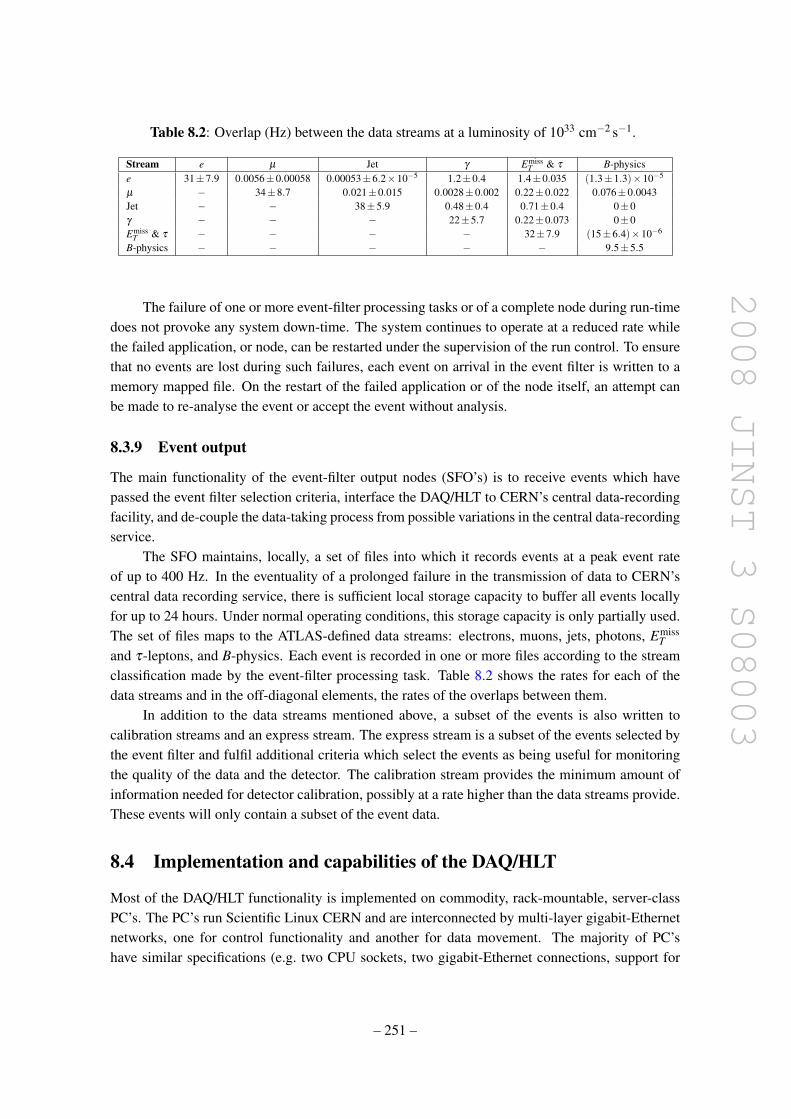
2008 JINST 3 S08003

Table 8.2: Overlap (Hz) between the data streams at a luminosity of 1033 cm−2 s−1.

Stream e µ Jet γ EmissT & τ B-physics

e 31±7.9 0.0056±0.00058 0.00053±6.2×10−5 1.2±0.4 1.4±0.035 (1.3±1.3)×10−5

µ − 34±8.7 0.021±0.015 0.0028±0.002 0.22±0.022 0.076±0.0043Jet − − 38±5.9 0.48±0.4 0.71±0.4 0±0γ − − − 22±5.7 0.22±0.073 0±0Emiss

T & τ − − − − 32±7.9 (15±6.4)×10−6

B-physics − − − − − 9.5±5.5

The failure of one or more event-filter processing tasks or of a complete node during run-timedoes not provoke any system down-time. The system continues to operate at a reduced rate whilethe failed application, or node, can be restarted under the supervision of the run control. To ensurethat no events are lost during such failures, each event on arrival in the event filter is written to amemory mapped file. On the restart of the failed application or of the node itself, an attempt canbe made to re-analyse the event or accept the event without analysis.

8.3.9 Event output

The main functionality of the event-filter output nodes (SFO’s) is to receive events which havepassed the event filter selection criteria, interface the DAQ/HLT to CERN’s central data-recordingfacility, and de-couple the data-taking process from possible variations in the central data-recordingservice.

The SFO maintains, locally, a set of files into which it records events at a peak event rateof up to 400 Hz. In the eventuality of a prolonged failure in the transmission of data to CERN’scentral data recording service, there is sufficient local storage capacity to buffer all events locallyfor up to 24 hours. Under normal operating conditions, this storage capacity is only partially used.The set of files maps to the ATLAS-defined data streams: electrons, muons, jets, photons, Emiss

Tand τ-leptons, and B-physics. Each event is recorded in one or more files according to the streamclassification made by the event-filter processing task. Table 8.2 shows the rates for each of thedata streams and in the off-diagonal elements, the rates of the overlaps between them.

In addition to the data streams mentioned above, a subset of the events is also written tocalibration streams and an express stream. The express stream is a subset of the events selected bythe event filter and fulfil additional criteria which select the events as being useful for monitoringthe quality of the data and the detector. The calibration stream provides the minimum amount ofinformation needed for detector calibration, possibly at a rate higher than the data streams provide.These events will only contain a subset of the event data.

8.4 Implementation and capabilities of the DAQ/HLT

Most of the DAQ/HLT functionality is implemented on commodity, rack-mountable, server-classPC’s. The PC’s run Scientific Linux CERN and are interconnected by multi-layer gigabit-Ethernetnetworks, one for control functionality and another for data movement. The majority of PC’shave similar specifications (e.g. two CPU sockets, two gigabit-Ethernet connections, support for

– 251 –

2008 JINST 3 S08003

Table 8.3: The main data-acquisition system components to be deployed for initial operation: thereadout system (ROS), the event-building node (SFI), the dataflow manager (DFM), the L2 super-visor (L2SV), the high-level trigger (HLT) and the event filter output nodes (SFO).

Component Number of Number of Number of Memory Type ofnodes racks CPU’s/node (Gbyte) CPU

ROS 145 16 1 0.512 3.4 GHz Irwindale

SFI 48 32 2 2.6 GHz Opteron 252DFM 12

1L2SV 10

HLT 1116 36 8 8 Xeon E5320 1.86 GHz

SFO 6 2 2 4 Xeon E5130 2.0 GHz

Monitoring 324

4 8 Xeon E5160 3.0 GHzOperations 20 2 4 Xeon E5130 2.0 GHz

IPMIv2.0), and differ only by the number and type of CPU’s implemented and the amount ofmemory. The main features per component and the number of nodes deployed for initial operationsin 2008 are given in table 8.3. A few components, the RoI builder, ROL and ROBIN, are, however,implemented in custom hardware.

The ROS PC’s are installed in standard ATLAS 52U racks, while all other PC’s are installed instandard 47U or 52U server racks. The number of racks (for initial operation) for each componenttype is given in table 8.3. In addition to the PC’s, each rack also contains a local file server andtwo gigabit-Ethernet switches. The latter form part of the multi-layered gigabit-Ethernet networkwhich implements the control and data networks. Each rack is also equipped with a water-cooledheat-exchanger, designed for the horizontal airflow within a rack, which provides up to 9.5 kW ofcooling power. The number of 1U PC’s per rack is typically just over thirty, constrained by coolingpower, power distribution (particularly in-rush current) and weight limits.

For initial operations, the DAQ/HLT system will be fully configured in the area of configura-tion, control and monitoring functionality. The operations PC’s are used to provide the various cen-tral services for configuring and controlling the trigger and data acquisition systems (e.g. run con-trol, error logging). The monitoring PC’s are used to monitor the system and sampled event data.

The initial system will also support full detector readout, over the 1574 point-to-point ROL’s,into the ROS’s at L1 trigger rates up to 75 kHz. The number of ROD’s, ROL’s and ROS’s perdetector TTC partition are given in table 8.4. Also given in this table is the expected size of eventdata per L1 trigger for each part of the detector for a luminosity of 1034 cm−2 s−1.

As described in section 8.3.7, the event-building functionality is performed by a set of SFI’sand scales linearly with the number of SFI’s, each SFI contributing 60 Hz and approximately90 Mbyte/s to the total event-building rate and aggregate bandwidth. For initial operations, forty-eight SFI’s are deployed allowing a sustained event-building rate of approximately 2.0 kHz, for anaverage event size of approximately 1.3 Mbyte.

– 252 –

2008 JINST 3 S08003

Table 8.4: Numbers of readout drivers (ROD’s), readout links (ROL’s) and readout systems(ROS’s) per detector TTC partition, as well as expected data size per L1A signal for a luminosityof 1034 cm−2 s−1.

TTC Partition Number of Number of Number of Data per L1A signalROD’s ROL’s ROS’s (kbyte)

Inner detector

PixelLayer 0 44 44 4

60Disks 24 24 2Layers 1–2 64 64 6

SCT

End-cap A 24 24 2

110End-cap C 24 24 2Barrel A 22 22 2Barrel C 22 22 2

TRT

End-cap A 64 64 6

307End-cap C 64 64 6Barrel A 32 32 3Barrel C 32 32 3

Calorimetry

Tile

Barrel A 8 16 2

48Barrel C 8 16 2Extended barrel A 8 16 2Extended barrel C 8 16 2

LAr

EM barrel A 56 224 20

576

EM barrel C 56 224 20EM end-cap A 35 138 12EM end-cap C 35 138 12HEC 6 24 2FCal 4 14 2

Muon spectrometerMDT

Barrel A 50 50 4

154Barrel C 50 50 4End-cap A 52 52 4End-cap C 52 52 4

CSCEnd-cap A 8 8 1

10End-cap C 8 8 1

L1

CalorimeterCP 4 8 1

28 (can be varied)JEP 2 8 1PP 8 32 3

Muon RPCBarrel A 16 16 2

12Barrel C 16 16 2

Muon TGCEnd-cap A 12 12 1

6End-cap C 12 12 1

MUCTPI 1 1 1 0.1CTP 1 1 1 0.2

Total 932 1574 145 1311

In addition to the features given in table 8.3, the PC’s for the SFO functionality are each equip-ped with three RAID controllers each managing eight 500 Gbyte SATA II disks. The three sets ofdisks are operated as a circular buffer: while events are being written to the event streams of one setof disks, a second set of disks is used to send data to CERN’s central data recording service. In thisconfiguration, a single RAID controller does not perform both writing and reading operations si-multaneously, thus maximising the throughput of an SFO. The deployed set of SFO’s fulfil the finaldesign specifications: a sustained output bandwidth of 300 Mbyte/s and a peak rate of 600 Mbyte/s.Thus for an average event size of 1.3 Mbyte, this gives a sustained event rate of 200 Hz.

– 253 –

2008 JINST 3 S08003

Of the 36 HLT racks available for initial operations, eight racks (248 nodes) are dedicatedto the event filter selection while the remaining twenty-eight racks (868 nodes) can be configuredto perform either the L2 trigger or event filter selection, i.e. the amount of computing power ap-portioned to the L2 trigger and or the event filter will be adjusted according to the data-takingconditions. The baseline apportioning of these nodes envisages nine racks (279 nodes) for the L2trigger and twenty-seven racks (837 nodes) for the event filter. In the DAQ/HLT Technical De-sign Report [237], the algorithm processing times and rejection rates were based on single-coreprocessors with an expected clock speed of about 8 GHz, giving processing times per event oforder 10 ms at L2 and 1 s at the event filter. These figures correspond to approximately 40 ms and4 s respectively per core on today’s quad-core processors operating at a clock speed of 2 GHz.Measurements with simulated raw data show that the processing times per event at L2 and eventfilter are consistent with the available computing resources for acceptable trigger rates and with arepresentative mixture of simulated events passing the L1 trigger. Therefore the system deployedfor initial operations should be able to handle an initial L1 trigger rate of approximately 40 kHz,about half of the final design specification.

8.5 Detector control system

In order to enable coherent and safe operation of the ATLAS detector, a Detector Control System(DCS) has been defined and implemented [238]. The DCS puts the detector hardware into selectedoperational conditions, continuously monitors and archives its run-time parameters, and performsautomatically corrective actions if necessary. Furthermore, DCS provides a human interface forthe full control of ATLAS and its sub-detectors. Figure 8.15 shows the general system architectureconsisting of two parts: the front-end systems and the back-end control.

The front-end consists of the hardware components used to control the detector, ranging fromsimple sensors to complex devices such as software controlled power supplies. In order to minimisethe effort of integration of devices into the DCS and to achieve a homogeneous system, a small setof commercial devices, such as crates or power supplies, has been selected as standard. The readoutof these devices is normally done using the industry-standard protocol OPC.

Due to the special conditions in the experiment cavern, strong magnetic field and ionisingradiation, a general-purpose I/O concentrator, the Embedded Local Monitor Board (ELMB) [239],has been developed. An ELMB comprises a multiplexed ADC (64 channels with 16 bit resolution),24 digital I/O lines and a serial bus SPI to drive external devices. The ELMB can be configured forvarious types of sensors. A micro-controller pre-processes the data (e.g. calibration, threshold de-tection) before they are transferred via CANbus to the back-end. The ELMB is designed and testedto be radiation tolerant to a level of about 1 Gy/y and can hence also be placed inside the detectorat places shielded by the calorimeter. The ELMB is used in two ways: either directly embeddedin the detector electronics, or attached to a general-purpose motherboard to which sensors can beconnected. In total about 5000 ELMB’s are installed and they are controlled by an OPC serverusing the CANopen protocol.

The back-end is organised in 3 layers: the Local Control Stations (LCS) for process controlof subsystems, the Sub-detector Control Stations (SCS) for high-level control of a sub-detectorallowing stand-alone operation, and the Global Control Stations (GCS) with human interfaces in

– 254 –

2008 JINST 3 S08003

Back-end

Gl b l C t l St ti (GCS)WWW

LHC Global Control Stations (GCS)

Data

viewerAlarm

system

Web

server

Operator

interfaceDCS IS

LHC

Services

Magnets

DSS

COOL

interface

Sub-detector Control Stations (SCS)

Data

bases

TilePixel SCT TRT MDT TGC RPC CSC CIC TDAQLAr

TDAQ

Run ControlID

USA15 L1 USA15 L2 US15 L2 SDX1

Local Control Stations (LCS)

UX15

Front-end

Cooling Racks Environment

Figure 8.15: Architecture of the DCS.

the ATLAS control room for the overall operation. Each station is a PC running the commercialcontrols software PVSS-II [240], which provides the necessary supervisory functions such as dataanalysis with the possibility of triggering the execution of pre-defined procedures, raising alarms,data visualisation, and archiving. This supervisory control and data acquisition software package(SCADA) has been chosen for all LHC experiments in the frame of the Joint Controls Project [241],which provides a set of tools on top of PVSS-II and also software components for the standardiseddevices. In total, the back-end consists of more than 150 PC’s, connected as a distributed system forwhich PVSS-II handles inter-process communication via the local area network. The full back-endhierarchy down to the level of individual devices is represented by a distributed finite state machineallowing for the standardised operation and error handling in each functional layer.

The LCS are connected to the front-end of a specific sub-system and read, process, andarchive the respective data. They execute the commands issued from the SCS and GCS layersand additionally allow the implementation of closed-loop control.

The SCS enable full stand-alone operation of a sub-detector by means of the finite statemachine and provide a user interface to control the different subsystems. The SCS also handles thesynchronisation with the data acquisition system.

The GCS in the top layer provide all functions needed in the ATLAS control room to operatethe complete detector. The operator interface shows the detector status and allows to navigate in thetree-like finite state machine hierarchy and to execute high level commands which are propagated

– 255 –

2008 JINST 3 S08003

to the layers below. A data viewer provides selection and plotting of all data available in the DCS.The alarm system collects and displays all parameters which are outside of pre-defined ranges,classified in three severity levels: Warning, Error, and Fatal. An information server (DCS IS)provides an interface to external control systems such as the sub-detector gas systems, the liquid-argon and helium cryogenics systems, the ATLAS magnets, and the electricity distribution for thedetector. The data collected from those systems is made available inside the distributed DCS to theindividual sub-detectors. Summarised status information is openly available via the World WideWeb.

In addition to the individual sub-detector control stations, one SCS is dedicated to CommonInfrastructure Control (CIC) to supervise the common environment and services of the detector.Each of the five geographical zones defined for the CIC (three electronics rooms underground,the cavern of the experiment, and the trigger and data acquisition systems computer rooms) iscontrolled by an LCS. In each zone, the environmental parameters are monitored, the operationalparameters of the electronics racks are supervised, and the electricity distribution is controlled.Furthermore, the CIC includes a large network of I/O points in the experimental cavern, consistingof about 100 ELMB’s. It reads the data of radiation monitors, the movement sensors of the safetysystem to look for personnel inside the ATLAS area (see section 9.9), and some 200 temperaturesensors positioned at the support structure of the barrel toroid. Additional readout capacity forfuture system extensions is available.

The DCS comprises a set of common software tools and packages, used by sub-detector con-trols and the CIC. A configuration database stores the settings needed for the different operationalmodes of the detector. All status information and measured data can be transferred to the ATLAS-wide conditions database COOL. Another package allows the synchronisation and informationexchange between the DCS and the data acquisition system.

– 256 –

2008 JINST 3 S08003

Chapter 9

Integration and installation

9.1 Introduction

The ATLAS detector has been installed underground in a huge cavern, situated in Switzerland atpoint 1 on the LHC ring, directly opposite the main entrance to the CERN site. The installationtask has involved a large team from across the whole collaboration (see annex 11.3).

The soil conditions at point 1 were favourable for the large amount of excavation work re-quired. Once the experiment was approved, preparations for the infrastructure began: civil engi-neering, electrical power distribution, cooling water, ventilation, etc. In parallel to the work on theinfrastructure, many studies on the assembly, integration, layout, support structures, services (pipesand cables), safety issues and access requirements/means for the experiment were carried out.

The construction of the component parts for ATLAS was distributed over many institutionsaround the world. The components then had to be brought to CERN in a timely manner, a consid-erable challenge in itself in terms of their size, complexity and fragile nature. In most cases, finalassembly and testing were done at CERN on the surface, prior to installation underground.

The main cavern is 92.5 metres underground and the detector is almost as large as the cavernin which it is housed. Supervising the construction of such a complex project meant that ratherformal and uniform management and engineering tools had to be used to monitor and documentthe progress of the project and ensure that items arrived on time and satisfied the requirements.Ensuring that all the pieces of the puzzle fitted together turned out to be a particularly difficultchallenge, since the physics goals and the geometry of the detector require minimal clearancesbetween neighbouring parts. One of the most stringent requirements of the ATLAS detector is toensure hermetic coverage over most of the solid angle: installation of the detector had therefore tobe performed to great accuracy, in order to guarantee optimal coverage.

After a brief description of the processes and tools used to fulfil the infrastructure, integra-tion and installation tasks (section 9.2), this chapter briefly describes the mechanical integration(section 9.3), the overall infrastructure and services at point 1 (section 9.4), the support and ac-cess structures (section 9.5), the detector installation process (section 9.6), the detector openingand access scenarios (section 9.7), the beam-pipe (section 9.8), safety issues (section 9.9), and theinterfaces to the LHC machine (section 9.10).

– 257 –

2008 JINST 3 S08003

Table 9.1: List and function of the various software tools used by ATLAS technical coordinationduring the installation of the detector.

Tool FunctionEngineering data management system (EDMS) Structured storage and retrieval of engineering dataCERN drawing directory (CDD) Processing of technical drawingsProject progress tracking (PPT) Regular Web-based notification and reporting systemEquipment management database (EMD)and manufacturing and test folder (MTF) database

Traceability of all equipment installed in the cavern

Rack wizard and ATLASeditor3D Configuration of electronics rack connectivity(from detector to counting room)

ATLASsurvey3D Monitoring of ATLAS sub-system displacements(also uses survey data)

Cable database Assist cable installation team(labels, routing, connector specifications, etc)

The Glance Project Interacts with all equipment dataresiding in distinct and geographically spread repositories

9.2 Organisational issues

The ATLAS project involves many people who are spread around the world. It has also generateda huge, complex and multi-disciplinary volume of data which needs to be organised and sharedin an easy and transparent way. The management of the integration and installation work was theresponsibility of the technical coordination team. In order to help manage the design, productionand installation phases of the ATLAS project, various organisational processes and computing toolswere developed [242]. The design phase of the project required the production of drawings, sched-ules and specifications for procurement. A number of review processes were included during thisphase of the project. The goal of these reviews was to evaluate the feasibility and technical validityof the proposed designs. In addition to these reviews, and before launching the production of majoritems, internal design reviews and production-readiness reviews were organised. Then, during theproduction phase of the sub-systems, production-advancement reviews were implemented to checkprogress and compare it with the production milestones in the schedule. In case of specific andmajor technical issues, experts were called in from within and outside the collaboration to solvesuch problems in a timely fashion.

The ATLAS technical management board meets on a monthly basis and provides a forumfor regular reporting of the status and problems in all areas relevant to the work at point 1 to thecollaboration scientists and engineers. During these meetings, the installation schedule is discussedand proposed future strategies are agreed upon. During the installation of ATLAS, the progressand status of the work were monitored on a weekly basis in dedicated meetings with each maindetector system. The Web-based tools shown in table 9.1 were used to assist in the communicationand organisation process.

– 258 –

2008 JINST 3 S08003

9.3 Mechanical integration

The mechanical integration process had to address both static issues related to installation andsurvey of major detector components and dynamic issues related to detector placement, movementsof parts during installation, and to access and maintenance (see section 9.7). This section deals withthe mechanical integration aspects related to installation.

The mechanical integration process defined the overall experimental layout, where eachnested sub-system has its well-defined shape and position and has no overlaps with any other sub-system. This integration process started from an initial input for the positioning of the sub-systemsand for the space needed for access and services. It then defined mechanical envelopes and theoverall three-dimensional layout of the ATLAS detector, using most of the tools listed in table 9.1.

9.3.1 Envelopes (individual, global, dynamic)

Envelopes define the space allocated to each part of each sub-system. Three types of envelopeshave been created, individual, global and dynamic, and they are defined as follows:

• The individual envelope is the space allocated for the manufactured object, including somespace added to the nominal design drawing envelope, in order to take into account fabricationand assembly tolerances.

• The global envelope includes, in addition to the individual envelope, some space dedicatedto the inaccuracy of the positioning inside the detector and the deformations applied duringinstallation and operation.

• The dynamic envelope includes, in addition to the global envelope, space for deviations anddeformations during displacements (e.g. during access) of the object inside the detector.

After the manufacture and installation of each sub-system, the envelopes were checked andcompared to the measurements performed by the survey team. Envelopes have been created as3D objects with the help of various CAD systems. All this work on modelling and conflict-checkinghas been most important in order to facilitate the installation process and avoid cost and scheduleproblems between conflicting objects during installation.

9.3.2 Survey and placement strategy

ATLAS is being assembled in a cavern which is not much larger than the detector itself. Thusany available space had to be optimised once an installation was complete. As soon as the cavernwas delivered to ATLAS by the civil engineers, and before any infrastructure was installed, anexhaustive scan was carried out in order to check the as-built work. The task of surveying for theATLAS detector has been a very challenging one due to the size, nature, complexity and globalscale of the work.

9.3.2.1 Survey reference grid in the cavern

The nominal beam-line was defined and used during the installation and positioning of the detectorsin the cavern. It is defined by the best-fit alignment line of the low-β quadrupole magnets, located

– 259 –

2008 JINST 3 S08003

at a distance of 30 m from either side of the interaction point. This reference line can deviate fromthe real beam-line by as much as 2-3 mm. It is determined by the reference sockets in the tunnel,from which the machine elements are installed. The final control is carried out on the machineelements themselves (inner focusing quadrupole triplets included) relative to each other. Spatialuncertainties from 0.5 mm to 1.2 mm at the one sigma level was estimated for any fiducial markwith respect to the nominal beam-line depending on the location of the given target.

The datum (interaction point, radial orientation of the colliding beams and reference plane)is given by the initial geometry in the tunnel and the final positioning of the low-β quadrupolemagnets. The survey grid reference in the cavern is linked to the machine geometry by stan-dard geometrical measurements and permanent monitoring systems. These include hydrostaticand wire positioning capacitive sensors, implemented in the survey galleries and joining the low-β quadrupoles via the cavern and radial tubes [243]. The reference grid will thus be monitoredthroughout the lifetime of the detector.

9.3.2.2 Stability measurements of the floor and the bed-plates

Aug 03 Feb 04 Aug 04 Feb 05 Aug 05 Feb 06 Aug 06 Feb 07 Aug 07

Ver

tical

dis

plac

emen

t (m

m)

-0.2

0

0.2

0.4

0.6

0.8

1

1.2

1.4 A23+10

A23+05

A23-07

A22-15

A17+08

A17-14

A11+05

B00-09

C23-07

C22-15

C17-14

C12-05

C12+05

Figure 9.1: Vertical displacements of the ATLAScavern floor, measured as a function of time invarious reference points since August 2003. Thebeam interaction point is at the origin (x = 0,z = 0). The labels used for the reference points arethe following: C23-7 represents a point on side Cat a distance of 23 m longitudinally from the in-teraction point and of 7 m radially opposite to thecentre of the LHC ring. In contrast, A23+10 rep-resents a point on side A at the same longitudinaldistance from the interaction point, but at a dis-tance of 10 m radially towards the centre of theLHC ring. The points labelled B are located rightin the middle of the cavern, nominally at z = 0.

Civil-engineering calculations indicated possi-ble vertical floor movements of up to 6 mm set-tlement due to the loading of the detector anda 1 mm per year lift due to excavation heave.ATLAS has a very limited adjustment capabil-ity once the detector elements have been placedin-situ. A placement strategy was therefore de-veloped to position all elements within the bestachievable mechanical tolerance, relatively tothe interaction point and the nominal beam-line [243].

To monitor these predicted movements,periodical measurements have been carried outon about 20 reference marks embedded in thecavern floor. The measurements are referencedto the machine levelling and to deep referencepoints in the tunnel.

In addition to these measurements, a per-manent hydrostatic system has been imple-mented in the ATLAS support feet bed-plates.It consists of six capacitive sensing stationsmonitoring the water plane in two 25 m longtubes, 55 mm in diameter, parallel to the beamand linked by a transversal tube. Two additional stations have been installed in the extremetrenches, recognised as stable zones, and linked to the bed-plate system. Altogether, this is equiva-lent to a reference water plane of 75 m length, inspected by eight sensors attached to the structure(bed-plate and stable floor) within an accuracy of better than 20 microns.

– 260 –

2008 JINST 3 S08003

The results from the measurements on the floor, as displayed in figure 9.1, show that, after aninitial stable period, during which presumably the heave of the floor was balanced by the loading,a global heave of the floor of up to 1.2 mm happened in the central part of the cavern betweenMarch 2004 and March 2006. By August 2006, approximately 85% of the total load had beeninstalled and, over the past 12 months, the cavern floor seems to have settled more or less and theupward heave is no longer visible.

The hydrostatic system in the bed-plates gives immediate movements of the supporting struc-ture with an accuracy of a few microns and has been used to monitor local movements wheninserting the calorimeters. It will now be operated continuously to monitor movements in real timeduring data-taking.

9.3.2.3 Placement of ATLAS sub-systems

The ATLAS detector had to be assembled in the main cavern mostly because of the nature of thebarrel toroid magnet structure, which is 26 m long and 20 m in diameter. As discussed above, onceassembled and cabled, the detector and its main components cannot in practice be adjusted anymore relative to the nominal beam-line. Careful consideration had therefore to be given to theoptimal placement of sub-systems during the assembly process. Many sub-systems were preparedon the surface, while others were prepared in the main cavern, prior to their installation in theirfinal position. The aim was to place all the detectors such that they will all be at their appropriatepositions relative to the nominal beam-line, once the installation is completed. In the process ofdefining the initial placements, the following input had to be taken into account:

• floor movement in the ATLAS main cavern (see above);

• deflections of the barrel toroid structures as they were loaded with the muon chambers andthe services passing throughout ATLAS;

• deviations of as-built dimensions with respect to the nominal ones for neighbouring sub-systems;

• deviations from nominal of the relative placements of different components, which wereinstalled as one assembly. For example, the solenoid and the LAr barrel electromagneticcalorimeter were assembled on the surface inside their common vacuum vessel with a non-negligible relative error with respect to their theoretical placement. When placing the wholeassembly in the cavern, the priority was therefore given to the solenoid regarding the relativeimportance of nominal placement for ATLAS operation;

• uncertainties on the position of the interaction point from the uncertainties on the closed-orbitcalculations and on the placement of the machine components.

Once an assembly of different sub-systems was completed, the relative position of its compo-nents was fixed. As the most prominent example, the barrel calorimeter assembly consists of: thebarrel tile calorimeter, itself assembled from 64 individual tile modules, the barrel LAr cryostat,which includes the solenoid, the barrel LAr electromagnetic calorimeter and the support rails forthe inner detector, located on the inner bore of the cryostat.

– 261 –

2008 JINST 3 S08003

Table 9.2: Placement accuracy and current average position along the vertical y direction of differ-ent components of the ATLAS barrel system. The average positions in y are given as an illustrationof the priorities set in the placement strategy between conflicting requirements from different com-ponents of the barrel system.

Assembly Component Placement accuracy (mm) Average position in y (mm)Barrel toroid 10 (all coils) Magnetic axis at −8

Barrel calorimetry Solenoid 2 Magnetic axis at −2.3Barrel calorimetry EM calorimeter (side A) 3 −3.1Barrel calorimetry EM calorimeter (side C) 3 −2.3Barrel calorimetry Cryostat 2 −0.1Barrel calorimetry Tile calorimeter 3 Axis at −0.5

ID pixel 0.2 −1.2ID barrel SCT 0.5 −1.3ID barrel TRT 0.5 −1.6

ID end-cap (side A) SCT 0.5 −1.9ID end-cap (side A) TRT 0.5 −1.6ID end-cap (side C) SCT 0.5 −2.4ID end-cap (side C) TRT 0.5 −1.6

The strategy for the placement of a given assembly was the following:

1. determine the best position for the assembly, taking into account the input described above;

2. after the initial placement was completed, survey the assembly as installed and perform ad-justments wherever possible to come as close as possible to the optimal position;

3. once a major component has been placed, update the envelope drawings to take advantageof the as-installed envelopes of the various components. In most cases, the components re-spected the assigned envelopes, and it was possible to recuperate some space, which wasused either to increase the stay-clear area between assemblies or to optimise further the po-sition of subsequent assemblies. In rarer cases, such as the barrel and end-cap inner detectorassemblies, the distance between the assemblies had to be increased by 5 mm with respectto nominal. These deviations are accounted for in the final detector description of the as-installed detector.

Table 9.2 shows the placement accuracies achieved along the vertical axis for the main com-ponents of the ATLAS barrel system relative to the nominal beam-line. Table 9.2 also shows themeasured offsets in the vertical direction, illustrating the priority given to the placement of thesolenoid as close as possible to the nominal beam-line and to the subsequent placement of theinner-detector components as close as possible to the nominal solenoid axis.

The placement accuracy along the beam-line is also in the few millimetre range, but thereare exceptions in some cases due to conflicts in envelopes between neighbouring sub-systems. Thecomponents of a given assembly are grouped together under the same heading to indicate clearlythat their relative position with respect to each other was determined prior to final installation.These relative positions are in many cases more precise than the overall placement accuracy of the

– 262 –

2008 JINST 3 S08003

Table 9.3: Placement accuracy and current average position along the vertical y direction of differ-ent components of the ATLAS end-cap systems.

Assembly Component Placement Average position in y (mm)accuracy (mm)

End-cap toroid (side A) 3 Align magnetic axis with barrel toroidEnd-cap toroid (side C) 3 Align magnetic axis with barrel toroid

End-cap calorimeter (side A) FCal 1 Align FCal symmetrically around beam-pipeEnd-cap calorimeter (side A) EMEC 3 −0.8End-cap calorimeter (side A) HEC1 3 −0.6End-cap calorimeter (side A) HEC2 3 0.5End-cap calorimeter (side A) Tile 3 −1.9End-cap calorimeter (side C) FCal 1 Align FCal symmetrically around beam-pipeEnd-cap calorimeter (side C) EMEC 3 −0.9End-cap calorimeter (side C) HEC1 3 −0.1End-cap calorimeter (side C) HEC2 3 −0.3End-cap calorimeter (side C) Tile 3 −0.4

Small wheels MDT/CSC/TGC 4 Align on nominal beam-lineBig wheels MDT/TGC 4 Align on nominal beam-line

End-wall chambers MDT 4 Align on nominal beam-line

assembly, as for example in the case of the SCT and TRT, or even as in the case of the pixels withrespect to the ID barrel, for which special care was taken to adjust the fixation points between thetwo sub-systems on the surface after assembly of the complete ID barrel in order to ensure thatthe geometrical axis of the pixel sub-system will be within 0.2 mm of the nominal beam-line. Itis also important to note that the placement of the ID components with respect to the inner warmvessel of the barrel cryostat has been surveyed with an accuracy of approximately 0.3 mm, whichis very similar to that achieved for the survey of the mapping machine used for the mapping of thesolenoidal field (see section 2.2.4).

In a similar way, albeit less complete because of installation work still ongoing in the end-capregions of the detector, table 9.3 summarises the positioning status of the end-cap calorimeters,the small wheels, the big wheels, the end-cap toroid magnets and the end-wall chambers. All theend-cap detectors can in principle be adjusted relative to the nominal beam-line, when the ATLASdetector is in the open position. In order to monitor possible small changes of detector positionsafter opening and closing the apparatus, an active optical system has been installed, which willprovide a precise monitoring (20 µm in the transverse plane and 100 µm along the beam) of therelative position of these components with respect to the barrel system.

The placement strategy explained above has been quite successful and all major ATLAScomponents are located well within the initial target of being aligned to within a few millimetresfrom the nominal beam-line at the start of data-taking.

More detailed information on the location of individual assemblies is kept in the various da-tabases and will be updated as movements are monitored over time. As an example, figures 9.2and 9.3 show the current deviations of the geometrical axes of the main components of the ATLAS

– 263 –

2008 JINST 3 S08003

z (mm)-4000 -3000 -2000 -1000 0 1000 2000 3000 4000

x (m

m)

-4

-3

-2

-1

0

1

2

3

4Solenoid magnet

Barrel tile calorimeterBarrel LAr calorimeter (positive z)Barrel LAr calorimeter (inner warm vessel)Barrel LAr calorimeter (negative z)

Barrel TRTBarrel SCTPixel

Figure 9.2: Deviations of geometrical axes of main components of the ATLAS barrel from nomi-nal. Shown are the deviations in mm in the x− z plane.

z (mm)-4000 -3000 -2000 -1000 0 1000 2000 3000 4000

y (m

m)

-4

-3

-2

-1

0

1

2

3

4Solenoid magnet

Barrel tile calorimeterBarrel LAr calorimeter (positive z)Barrel LAr calorimeter (inner warm vessel)Barrel LAr calorimeter (negative z)

Barrel TRTBarrel SCTPixel

Figure 9.3: Deviations of geometrical axes of main components of the ATLAS barrel from nomi-nal. Shown are the deviations in mm in the y− z plane.

– 264 –

2008 JINST 3 S08003

barrel from the nominal beam-line, respectively in the x− z and y− z planes. Since the full loadingof the detector in the barrel region, a larger than expected compression of the support feet has beenobserved. This has led to a 1.5 mm downward shift of the whole barrel, as can be seen more pre-cisely from the average y-positions of the axes of the inner-detector sub-systems in figure 9.3. Allthese initial positions are recorded in the overall database and they will be monitored with timeas soon as new survey numbers become available or as the access and maintenance scenarios willrequire.

It will also be necessary to monitor the global movements of the detector to understand pos-sible future deviations in position between the detector and the actual beam. In the case of suchdeviations at the level of 1 mm, the beams can be adjusted and steered, using the field in the tripletmagnets and/or adjusting the position of the last magnet. In the event of larger movements, it willbe necessary to adjust the magnets over the last 300 m on either side of the interaction point. It hasbeen expected that such an exercise can be done once every three to four years.

9.4 Infrastructure and detector services

This section describes the infrastructure for the surface and underground areas and the services,fixed and mobile, which are connected to the ATLAS detector [244].

9.4.1 Civil engineering

The civil engineering work for the ATLAS experimental area started in November 1997 whilst theprevious accelerator (LEP) was still in operation and the situation remained so until the end of 1999.The work included the excavation and concreting of two new shafts, two new large caverns alongwith the linking galleries, and the construction of six new buildings on the surface, as shown infigure 9.4.

The underground work included the excavation and concreting of the following:

• The PX14 and PX16 shafts, respectively 18 m and 12.6m in diameter, both 60 m deep.

• The PX15 shaft was an existing shaft that required concreting only.

• The main cavern UX15 (50 m long, 30 m wide and 35 m high), which houses the ATLASdetector. Due to the continued operation of LEP in 1999, the vault had to be concretedbefore the support walls were put in place, leading to a non-standard anchoring technique ofthe 7000 t roof of the UX15 cavern. UX15 was delivered to CERN for the installation of theinfrastructure in June 2003.

• The counting room and service cavern USA15, which houses the electronics racks and ser-vices that need to be close to the detector and is accessible during machine runs.

• The seven linking galleries for personnel access and the distribution of services between theUX15 and USA15 caverns.

The surface buildings include the following:

– 265 –

2008 JINST 3 S08003

Figure 9.4: Layout of surface buildings and of access shafts to the ATLAS cavern at point 1. Themain areas of underground activity are the main cavern (UX15) and the main counting room andservice cavern (USA15). The main control room is in building SCX1 on the surface.

• SX1, a steel frame building located on top of the main shafts and housing the travellingcranes, maximum 280 t capacity. Used as short term storage of detector components, priorto their lowering into the main cavern. It also acts as a shelter from the external environmentand allows better control of the conditions in the cavern. This building was the first to bestructurally achieved allowing the infrastructure works to take place in dry conditions.

• SDX1, located on top of the personnel access shaft and used for the personnel and materialaccess control to the underground areas. It also contains the uninterruptible power suppliesfor the detector services, an electrical sub-station, and the DAQ room.

• SUX1, the ventilation building, containing the water chillers and air-conditioning units forthe underground areas and the new surface buildings.

• SCX1, the main ATLAS control building, used during the detector assembly phase as anengineering design office.

• SH1, a concrete building, containing the noisy cryogenic compressors and other cryogenicequipment.

• SF1, the new cooling towers for the final dissipation of heat recovered from all the under-ground areas and surface buildings via the water cooling circuits.

– 266 –

2008 JINST 3 S08003

Figure 9.5: Air ducts installed for ventilation in the shaft and main cavern.

9.4.2 Electrical power distribution

The total electrical power required on the ATLAS site at point 1 is about 13 MW, which has resultedin the installation of a new 66 kV sub-station, the reorganisation of the existing 18 kV sub-station,and a new 3.3 kV sub-station. Some 21 new transformers with a total power of 42 MW havebeen installed both on the surface and underground to bring the 3 kV or 400 V/230 V power to allATLAS systems.

There are different power networks to deal with the appropriate levels of continuous and safeoperation:

• Assured power: the normal power is backed up by two diesel generators of 1 MW each,located on the surface;

• Secured power: the technical solution is as for assured power, but it is not interrupted whenemergency stop buttons are activated;

• Un-interruptible power: these very critical systems are fed by battery back-ups with a totalpower of approximately 700 kW.

9.4.3 Air-conditioning and cooling systems

The global environmental requirements in the bulk of the ATLAS cavern are driven by generalconsiderations and by more specific ones from the muon spectrometer chambers. The temperatureshould remain stable at 25±3C and the humidity should be between 25% and 60%. The coolingand ventilation installation was one of the first infrastructure items to be installed, once the surfacebuildings had been handed over to CERN, in order to rapidly provide ventilation to the underground

– 267 –

2008 JINST 3 S08003

Table 9.4: Overview of main characteristics of the major cooling systems operating in the ATLAScavern.

System Medium Capacity (kW) Channel count Operatingtemperature (C)

Tile calorimeter Water 55 24 cooling loops supplying 17 to 22256 tile fingers

LAr calorimeter Water 250 24 cooling loops supplying 17 to 2260 electronic boxes

Diffusion pumps Water 50 12 cooling loops supplying 14 to 1926 diffusion pumps

Muon spectrometer and Water 300 26 cooling loops supplying CSC’s 17 to 22general-purpose stations plus racks for small and big wheels

ID evaporative C3F8 60 4 distribution areas supplying -30 to 10(pixel and SCT) 204 cooling channels

ID mono-phase (TRT) C6F14 70 4 distribution areas supplying 14 to 22176 cooling channels

ID mono-phase (cables) C6F14 80 32 distribution manifolds 14 to 22placed all over the detector

areas. This installation included new cooling towers in SF1, the liquid chillers in SUX1, 16 air-handling units in SUX1, SDX1, SX1, and USA15 and kilometres of water pipes and air-ducts. Thesystem is able to cope with emergency cases in fast-extraction mode (see section 9.9).

One of the most challenging tasks was the installation of air supply and extraction ducts inthe PX14 shaft, as shown in figure 9.5, and on the vault of the UX15 cavern, this system havingthe task of extracting the 200 kW of heat released into the air of the cavern by the ATLAS detector.The air-conditioning system has been up and running since summer of 2004. Provision has beenmade for thermal screens to be incorporated inside the detector to prevent a too large temperaturegradient across the inner layer of muon chambers.

Table 9.4 summarises the characteristics of the main cooling systems used for extracting theheat from the detector itself (silicon-sensor leakage currents and ionisation in the TRT gas, assummarised in table 4.10), from the on-detector and off-detector electronics, and from dissipationin the power cables. Most cooling systems are leakless by design and the inner detector has chosenfluorinert systems to minimise risks to the detector in case of leaks. In the case of the pixel andSCT sub-systems, a novel and complex evaporative system has been designed and brought intooperation to minimise the amount of material devoted to cooling pipes, fluids and connectors onthe detector itself. The detector-specific cooling systems are installed in the USA15 side cavernand have been brought into operation in 2005 and 2006.

9.4.4 Gas distribution

The ATLAS detector requires a variety of gases for its normal operation. Table 9.5 summarises thecharacteristics of the main gas systems used for normal operation.

The surface gas building SGX1 was designed for the storage, distribution, and mixing of in-ert and flammable gases in accordance with the CERN regulations. The building was completed

– 268 –

2008 JINST 3 S08003

Table 9.5: Overview of main characteristics of the gas systems operating in the ATLAS cavern.

System Gas mixture Pressure (bar) Volume (m3) Channel count Impurity limitsTRT active gas Xe/CO2/O2 1.005 2.5 (detector) 48 for barrel < 100 ppm CF4

(normal operation) 70/27/3 2.0 (gas system) 14 per end-capTRT active gas Ar/CO2/CF4 < 100 ppm H2O

(cleaning mode) 70/26/4TRT ventilation CO2 1±0.001 2.9 48 < 100 ppm H2O(flushed to atm.) (barrel)

TRT cooling CO2 1±0.001 6.0 4 < 1% N2

(closed loop) (end-cap) < 100 ppm H2OSCT ventilation N2 1.004 4 < 350 ppm H2O(flushed to atm.)Pixel ventilation N2 1.004 1 < 350 ppm H2O(flushed to atm.)

ID ventilation CO2 1.0005 13 < 1% N2 in ID(flushed to atm.)MDT active gas Ar/CO2/H2O 3 (abs.) 710 112 for barrel < 100 ppm O2

93/7/(≤ 1000 ppm) 81 per end-capCSC active gas Ar/CO2 1±0.001 0.5 32 < 100 ppm O2

80/20RPC active gas C2H2F4/Iso-C4H10/SF6 1±0.001 14 128 < 1% O2

94.7/5/0.3 < 100 ppm H2OTGC active gas CO2/n-pentane 1±0.001 16 128 for active < 5 ppm at entrance

55/45 56 for CO2 purge of n-pentane liquefier

in 1997. Large quantities of liquid gases are stored, both inside and outside this building, in par-ticular N2, CO2, Ar, Xe, He, C2H2F4, CH4, C4H10, and n-C5H12. The building is also fitted withan anti-deflagration roof, mechanical ventilation, permanent gas extraction and gas detection, andan alarm system. The mixing room contains the mixing systems for the different sub-detectors.The TRT, MDT’s, CSC’s and RPC’s use non-flammable gases. Only the muon TGC’s will useflammable gas (CO2/n-pentane).

The underground installation consists of a large network of stainless-steel pipes, which con-vey the gases to the gas room located in the USA15 cavern and then to the gas racks in the maincavern. From the gas racks, many kilometres of pipes have been installed. They connect to all thedifferent types of muon chambers (see section 6.9.1) and to the inner detector (see section 4.2.2).

9.4.5 Cryogenic systems

The ATLAS detector includes two independent systems requiring cryogenic technologies: the su-perconducting magnets and the liquid argon calorimeters. The cryogenic systems for the magnetsand the LAr detectors have each been divided into three parts:

1. External cryogenics, which comprise all the equipment needed to provide the required cool-ing capacity at given temperature levels, including refrigeration plants and infrastructure.This equipment is located on the surface in the SH1 building and underground in the USA15cavern. Also, six large helium gas storage tanks (3 m diameter, 21 m long) have been in-stalled on the surface behind the SX1 building.

– 269 –

2008 JINST 3 S08003

2. Proximity cryogenics, which comprise all the equipment linking the internal cryogenics tothe external cryogenics. This equipment is located in the main cavern, on the steel structure(HS) that surrounds the detector (see section 9.5).

3. Internal cryogenics, which comprise all the devices located inside the system concerned(magnets or liquid argon calorimeter).

The cryogenics systems for the magnets are described in some detail in section 2.1.4.2. Thissection is devoted to a brief description of the cryogenics systems for the LAr calorimeters.

The primary cooling source for the LAr calorimeter installation is a 20 kW nitrogen refriger-ator, which operates at 80 K. Under normal circumstances, the LAr cryostats are filled only onceand the liquid argon is never replaced. The argon is kept in the liquid phase by cooling it withliquid nitrogen (which has a slightly lower boiling point than argon) circulating in cooling pipessurrounding the calorimeters. These cooling pipes are also used during the cooling down of thecryostats. The flux and pressure of the liquid nitrogen are regulated such that its boiling pointtemperature corresponds to the cooling power required to keep the liquid argon at its operatingtemperature.

The compressor station is placed in the SH1 surface building and the cold box in theUSA15 side cavern. The high- and low-pressure gas lines connecting these two items pass throughthe PX-15 shaft. The cold box delivers its cooling power to a 15,000 litre phase-separator dewarplaced in the main cavern. Two 50,000 litre liquid nitrogen storage tanks placed on the surface willsupply liquid nitrogen to the phase-separator dewar via a 283-metre long transfer line, in case ofproblems with the nitrogen refrigerator system. A cryogenic centrifugal pump circulates the liquidnitrogen from the phase-separator dewar through the thirteen heat exchangers placed in the liquidargon cryostats. Each cryostat has been equipped with a valve box, which regulates the mass flowand pressure of the liquid passing through each of the individual heat exchangers. These valveboxes are placed on the HS surrounding structure.

The gaseous nitrogen coming from the heat exchangers is returned to the phase-separatordewar and from there returned to the nitrogen refrigerator system or, in case it is not operational,vented to the surface through a 120-metre long gas line. The three cryostats, placed at the heartof the detector, are linked by large-diameter argon lines to their individual expansion vessel placedon the HS structure. The liquid/gaseous argon boundary of each of the cryostats is located in theseexpansion vessels.

The need to move the calorimeter end-cap cryostats over a 12 m distance required the imple-mentation of a movement system for the argon and nitrogen lines connecting these cryostats withtheir expansion vessels and the nitrogen regulation valve boxes. These movement systems are lo-cated on the HS structure and are described in section 9.7. Figure 9.6 shows the underground layoutof the proximity and external cryogenics for the LAr calorimeters (shown as if installed alone forconvenience). One can clearly see the fixed cryogenic lines supplying the barrel calorimeter at thetop and also the cryogenics lines in the flexible chains, which supply the two end-cap calorimetersand which follow them whenever they have to move for access and maintenance of the detector.

The 84 m3 of liquid argon present in the cryostats can, in the event of problems, be emptiedby gravity into two 50 m3 argon storage tanks placed at the lowest point of the main cavern. A

– 270 –

2008 JINST 3 S08003

Liquid argonstorage tanks

Nitrogenphase separator

Valve boxExpansion vessels

Figure 9.6: Layout of the underground external and proximity cryogenics lines for theLAr calorimeters.

DN500 safety valve line collects any gas coming from the pressure safety valves placed on thecryostats, or storage tank volumes venting it to the surface.

9.4.6 Racks and cables

Prior to the start of the civil engineering work, the detailed cabling and rack needs were not known.The consolidated data from the various sub-systems was provided only much later and the correctprovisions for the distribution of cables from the detector to the electronics racks in the countingroom and service caverns were therefore made just before the start of the installation work. Theseincluded:

• locations for 100 racks in the main cavern, supported from the HS steel structure whichsurrounds the detector;

• the arrangement of the service cavern and counting room (USA15) with provision for250 racks on two floors, equipped with a 2.5 MW water-cooling system;

– 271 –

2008 JINST 3 S08003

• two main cable distribution galleries, which connect the main cavern to the counting roomwith provision for 44 cable trays, each 600 × 100 mm2 in cross-section;

• the distribution of these 44 cable trays on the HS supporting structure around the perime-ter of the detector and to the HO supporting structure on the end-walls of the cavern (seesection 9.5).

• locations for 70 racks in another service cavern (US15) together with about 20 holes, each300 mm in diameter, through the 2 m-thick connecting wall for the passage of cables, withthe associated cable-tray distribution system in the existing false floor and with a dedicatedcooling system of 500 kW capacity;

• locations for 100 racks in a self-contained data-acquisition room in the SDX1 surface build-ing with a 500 kW total water-cooling capacity and a dedicated 100 kW air-conditioningsystem.

Figure 9.7: Quantities of cable and flexible-pipebundles installed by the cabling team.

The various electronics units for the de-tector are thus installed in racks, implanted inUSA15, UX15 and US15 in the undergroundareas, and in the data-acquisition room on thesurface. The total number of racks (electronics,gas and water) for ATLAS amounts to approx-imately 500. The Rack Wizard tool mentionedin section 9.2 is essential to monitor the evolu-tion of the racks with time. The power require-ments, specific contents and the connectionsare constantly updated as they evolve: this isrequired not only for the maintenance of thedetector and the understanding of its evolutionon the long term, but also to meet (InstallationNucléaire de Base) regulations (see section 9.9).

It was necessary to design new types of racks with respect to what existed in the previousprojects, due to the increased power consumption, which therefore required more cooling capacity.The rack cooling is provided by turbine units located at the top of the racks, which push the airdown in ducts at the sides of the racks. A deflector at the bottom directs the air upwards throughthe equipment to be cooled, which is interspersed with heat exchangers. The turbine units comprisean ELMB-based monitoring system (temperatures, humidity, air flow, etc.), which is supervised bythe common infrastructure control of the DCS (see section 8.5). It was also found useful to increasethe width of some racks. All these requirements have led in the end to the production of four typesof racks, from 46 to 57 units in height, from 900 to 1000 mm in depth, and 600 mm in width.

Most of the installed cable trays are made of stainless steel to minimise the perturbations tothe magnetic field (see section 2.2.2). A total of about 50,000 cable bundles, 3000 flexible pipesand 3500 metallic pipes (see figure 9.7) were installed over a period of two years (May 2005 toMay 2007). Many additional proximity cables were installed by the individual sub-systems. Spacehad to be found to route the large quantity of cables and pipes of the inner detector and barrel

– 272 –

2008 JINST 3 S08003

Figure 9.8: Detailed three-dimensional layout and routing of cables and services for the ATLASbarrel system. The three flexible chains for the end-cap calorimeters can be seen in the horizontalplane (right) on the side where the end-cap calorimeter trigger cables can reach the main servicecavern (USA15) along the shortest possible path, and at 45 below the horizontal plane. One alsosees the cryogenic lines for liquid argon at the top and bottom of the drawing. The inner barrelmuon chambers in the central region are shown. One clearly sees the holes in the acceptancecaused by the considerable volume of services exiting the detector at z ∼ 0.

calorimeter systems through the muon spectrometer; this was accomplished by routing most ofthem radially outwards at z = 0 and at fixed azimuthal locations, as illustrated in figure 9.8. All therelevant cable and pipe data are stored in the cable database and constantly updated for the samereasons as those described for the racks above.

9.4.7 Drag-chains and mobile services

Many of the ATLAS sub-systems must move away from the run position to allow access intothe detector. As well, the end-cap calorimeters need to remain in a cold bath of liquid argon forthe duration of the experiment. The end-cap toroids are cooled with liquid helium and these arealso to remain cold during the movement to avoid the lengthy cool-down and warm-up periods(20 to 40 days).

In order to satisfy the above requirements it was decided to use so-called drag-chains, whichallow for the services to be supported in a flexible structure. They are used as follows:

– 273 –

2008 JINST 3 S08003

• For each end-cap calorimeter there are three chains, as shown in figures 9.8 and 9.9, non-standard commercial products, each around 30 m-long with parts in stainless steel, specif-ically developed for this application. They also have a force-assist system that enables thechain to be pulled back into its stored position when the calorimeter is being closed. Particu-larly challenging was the construction of two of the three chains, which are at 45 downwardswith respect to the beam axis.

• For each muon inner layer (small wheel) there are four chains, each about 3 m in lengthinside the ATLAS detector.

• For each end-cap toroid there are two chains. These are in aluminium and have been custommade. They run unsupported over a 9 m length at 24 m from the floor when the toroids aremoved to their fully open position off the beam axis.

9.4.8 Grounding and electromagnetic compatibility

Figure 9.9: The end-cap calorimeter on sideA in its fully open position with all three drag-chains and the flexible LAr fill-line connected.

The ATLAS detector consists of many complexcomponents, installed and operating in contigu-ous volumes, resulting in a large amount of in-stalled equipment with multiple interconnectionsand shared services. For these reasons, the per-formance of the detector components could beheavily affected by electromagnetic interferenceor induced electronic noise, if these issues are notproperly taken care of already at the design stageand systematically followed up on during instal-lation. This is particularly important for detectorsystems with a large dynamic range and with ana-logue front-ends and/or readout.

An ATLAS policy was developed andadopted already in the design phase [127, 245]to minimise possible electromagnetic interferenceeffects. Apart from safety considerations, oneof the main concerns has been the prevention ofground-loop currents which could couple to thesignals of the detector systems. The proposed im-plementation of the ATLAS policy on groundingand electromagnetic compatibility has been putin place during the construction and installationphases [128]. The main guidelines can be sum-marised in three rules: all detector systems areelectrically isolated, there are no connections toground other than through the safety network, and there are no connections between different de-tector systems.

– 274 –

2008 JINST 3 S08003

Even though these rules have been implemented and validated early on in the design phase, ithas been a challenge to preserve the electrical isolation of certain large systems during installation.For these reasons, several alarm systems [128] have been installed and operated to ensure that thevarious detector components remain electrically isolated and grounded to single points. This effortwas especially relevant for large structures with many connections like the LAr cryostats, whichact as a support for other detector elements and are themselves supported by other parts of ATLAS(see section 5.6.1.1).

9.5 Support and access structures

9.5.1 Feet and rail system

The feet and rail system is shown in figure 9.10 shortly after installation in the pit and before thelowering of the first barrel toroid coil. This system is the main support, the back-bone, of theATLAS detector. It is made of nine pairs of feet, bound by girders that altogether support the twobottom coils of the barrel toroid magnet. On top of these feet are two rails, and their supports, onwhich the central part of ATLAS can slide. The total load that the feet and rail system has to copewith is about 6000 t (of which approximately 1000 t correspond to the barrel toroid, which is onlysupported by the feet). The feet and rail system is mounted on bed-plates, which give the detectorits 1.24% incline with respect to the cavern floor, an angle which matches the inclination of theLHC accelerator tunnel.

Since the two bottom toroid coils are placed inside the feet, there was a strong requirement forthe material to be non-magnetic. In addition, the total deformation was to be kept to a minimum,and stresses well below the elastic limit. Low-carbon austenitic stainless steel was chosen for itsgood mechanical properties and very low magnetic permeability. One of the main technical issueshas been to produce non-magnetic welds for such a huge number of welded joints (up to 15 t offiller metal in total).

In order to obtain a precise and reproducible geometrical path of the loads during the move-ment of the sub-detectors on their air-pad movement systems (see section 9.7.2), and also to pre-serve the integrity of the beam vacuum system (see section 9.8), the flatness requirement on therails was one millimetre over their total length (more than 25 m), and 0.2 mm over any length ofone metre. The maximum deflection of the system remains below 1 mm during the movement ofthe loads.

The requirement to preserve maximum acceptance for the muon spectrometer resulted inspecial chambers in the region of the feet and additional chambers alongside the rails (see sec-tion 6.3.2). Numerous improvements in the feet design were introduced to cope with constraintsfrom the muon alignment system, with various designs of the muon support rails, as well as withthe barrel toroid magnet instrumentation and contact surfaces.

9.5.2 Trucks

The so-called HF trucks are normal steel structures, which are placed directly below the two shaftsof the main cavern. They allow for the main components of the detector to be lowered underground

– 275 –

2008 JINST 3 S08003

Figure 9.10: The ATLAS feet and rail system after installation and prior to the installation of thefirst barrel toroid coil. Also shown are the blue steel surrounding structures (HS and HO), and, inthe background, one of the orange HF trucks.

using the surface cranes and remain there temporarily before moving into their final position, eitherby using the cavern travelling cranes (as for the barrel toroid magnet coils) or by using the air-padmovement systems (as for the calorimeters).

These structures also have the role of supporting the end-cap toroid magnets, as well as theend-cap calorimeters, in the opening sequences of the ATLAS detector (see section 9.7). Duringinstallation, they also support the forward shielding, whereas they will only support part of it whenit is inserted in its final location. They are therefore able to cope with the 1000 t of maximumstatic load from the barrel calorimeter and they have to allow for the translation of the end-captoroid magnets and of the forward shielding away from the beam (total weight of 400 t). For suchmovements, air-pads will be attached to the base of these structures to allow them to slide on thecavern floor.

– 276 –

2008 JINST 3 S08003

Figure 9.11: The blue support structures (HS on the sides and HO at the ends of the main cavern)at the beginning of ATLAS installation. The arches which now connect the two sides of HS at thetop of the main cavern were left out at the time for the installation of the barrel toroid. A barreltoroid coil is in the process of being lowered onto its temporary supports (see section 9.6).

9.5.3 Surrounding structures (HS and HO)

The blue HS structures, which surround the ATLAS detector, as shown in figure 9.11, have dualroles of providing personnel access to the periphery of the detector and to support all the equipmentthat has to be located close to the detector: proximity cryogenics, electronics racks, gas-distributionracks, electrical switchboards, and services distribution lines (gas, water, coolants, power). Thesestructures were the most tricky to assemble, since they are very close to the detector in certainplaces and had to be assembled in two stages: the large pillars and gangways up to a height of 20 mwere installed at the same time as the HO structures, but the tops of the HS arches were installedonly after the completion of the installation of the barrel toroid magnet and with very little marginleft. The two structures, which span distances of more than 20 m in three dimensions had to matcheach other to within 2 cm. The last arch was finally and successfully installed at the end of 2005.

The main role of the HO structures, which are to be found at the two ends of the cavern, areto support the end-wall muon chamber stations. They also serve as a useful means of assemblingthe sectors of the muon big wheels, before they are hung from the rail system. These structuresalso serve as viewing platforms for the thousands of visitors to the ATLAS cavern . Approximately1000 t of normal steel have been used to build these 13-storey-high structures.

– 277 –

2008 JINST 3 S08003

9.5.4 Muon barrel access structures

The aluminium access platforms inside the barrel muon spectrometer have several functions:

• permanent access inside the barrel toroid, so that the muon chambers and their service con-nections can be accessed in a very short intervention (for example, to disconnect the gassupply to a specific chamber);

• permanent access to the patch-panels of the inner detector (PP2), so that they can also beaccessed during a very short intervention;

• an emergency exit (through sector 1) in case of access to the barrel calorimeter;

• access for the installation of the barrel muon chambers;

• access to the vacuum pumps of the barrel toroid.

9.5.5 Big wheels

The muon spectrometer (see section 6.1) includes four big moving wheels at each end, each wheelmeasuring 23 metres in diameter (see figure 9.12). Of the eight wheels in total, six are composedof thin-gap chambers (TGC’s) for the muon trigger system and the other two consist of moni-tored drift-tube chambers (MDT’s) to measure precisely the position of the muons. The so-calledbig wheels comprise aluminium structures which support the muon end-cap chambers. These bigwheels resemble bicycle wheels and are made of sectors, which had been pre-assembled on thesurface prior to their transport to the cavern, where they were assembled on the end-wall HO struc-tures. Once one of the wheels is completed on the HO structure, it is lifted onto the traction system,which allows it to move longitudinally towards the barrel toroid magnet and reach its final positionin the closed configuration of the detector. It is important to note that the big wheels in their finalposition need to be inclined with a slope of 1.24% with respect to the vertical to account for theangle between the horizontal cavern floor and the inclination of the machine tunnel.

9.6 Detector installation

The installation of the detector can be sub-divided into six main phases, which are briefly describedbelow. The barrel toroid magnet, once installed, occupies the central region of the cavern leavingthe two sides, A and C, for the lowering and assembly of the remaining large detectors and magnets.

9.6.1 Phase 1: infrastructure in the main cavern, feet and rails

The main cavern was handed over to ATLAS in May 2003. The first operation was to installthe general infrastructure (metallic structures around the cavern walls, temporary electricity andlighting, ventilation ducts, and the overhead travelling cranes).

With the steel structures installed, the first elements of the ATLAS detector to be broughtdown were the bed-plates, which were bolted to the concrete cavern floor. After the bed-plates,the stainless steel support feet, 18 in total, were lowered one by one and installed. The main rails

– 278 –

2008 JINST 3 S08003

Figure 9.12: One of the assembled TGC big wheels in the ATLAS cavern. The chambers are fixedto an aluminium structure, which was pre-assembled into sectors on the surface and then assembledas a complete wheel in the cavern itself.

were installed and surveyed once positioned on the feet. The feet provide the mechanical supportfor most of the ATLAS sub-systems, namely the barrel toroid magnet, the calorimeters, the barrelmuon chambers, the end-cap toroid magnets, the services and the access structures, amounting toabout 6000 t.

9.6.2 Phase 2: barrel calorimetry and barrel toroid

Side A: barrel toroid. The first barrel toroid coil was delivered to point 1 in October 2004. Thecoil with its weight of 100 t and total length of 25 m, was lifted by the surface crane, tilted withhydraulic winches, lowered, in an inclined orientation, through the 18 m diameter shaft down intothe cavern. It was then turned back to the horizontal orientation, before being lowered onto thetemporary supports (see figure 9.11). From there, it was picked up by the two 65 t undergroundtravelling cranes and put into its final position inside the ATLAS feet. Once the coils were inposition, the aluminium struts and girders were installed so that the next coil could be attached tothem. This process was repeated until the assembly was completed. In parallel with the barrel-toroid assembly, the first 100 muon barrel chambers were installed in between the struts/girdersand the ATLAS feet.

– 279 –

2008 JINST 3 S08003

Figure 9.13: Lowering of the barrel LAr calorimeter down to the cavern in October 2004. Thefirst barrel toroid coil can also be seen on a temporary support platform before it is installed in thecradles of the feet.

Side C: barrel calorimeter. The lower part of the tile calorimeter was lowered in March 2004.Individual tile calorimeter modules were then assembled together, one by one, until 32 of the64 modules were completed. The LAr barrel calorimeter cryostat was then lowered into this half-cradle in October 2004, as shown in figure 9.13. The tile module assembly was then continueduntil the mechanical assembly of the full barrel calorimeter was completed.

Barrel: completion of barrel toroid and calorimeter installation. The last aluminium girderwas put in place in September 2005, completing the mechanical assembly of the barrel toroid struc-ture. Then the hydraulic jacks, which were supporting the complete structure during the assembly,were released. At this moment the load was transferred from the external temporary supportingstructure (used during the magnet assembly) to the support feet at the bottom. The temporary sup-port structure was then cut and removed to give space for the barrel calorimeter, which was movedinside the barrel toroid in October 2005.

9.6.3 Phase 3: end-cap calorimeters and muon barrel chambers

Side C: end-cap calorimeter. With the barrel calorimeter installed inside the bore of the magnet,the space on side C was now vacant for the assembly of the first end-cap calorimeter. This assemblywas very similar to that of the barrel and was finished in January 2006. It was then moved insidethe barrel toroid in February 2006, once the installation of the services (pipes, cables, etc.) wascompleted.

– 280 –

2008 JINST 3 S08003

Figure 9.14: View of installed barrel muon spectrometer stations and end-cap calorimeter onside A.

Figure 9.15: View of barrel calorimeter and inner-detector end-flange after installation of the firstinner-detector end-cap in early June 2007 (left). This was followed shortly thereafter by the instal-lation of the second inner-detector end-cap and of the pixel detector with the central VI section ofthe vacuum pipe (right).

Side A: barrel muon chambers and end-cap calorimeter. On side A, the first of the 656 bar-rel muon chambers was installed in February 2006. When the assembly of the second end-capcalorimeter started in March 2006, it had to be carried out in parallel with the muon-chamber in-stallation. The second end-cap calorimeter was mechanically completed in May 2006. It stayedoutside the barrel toroid for a further two months for the installation of the services while the end-cap calorimeter on side C was moved to its nominal position and the magnetic field of the solenoidwas switched on and measured in June 2006 (see section 2.2.4).

– 281 –

2008 JINST 3 S08003

9.6.4 Phase 4: muon big wheels, inner detector and completion of muon barrel

Figure 9.16: Lowering of the first end-cap toroidmagnet onto the truck on side A in June 2007.One of the TGC big wheels can be seen on theright of the picture.

Side C: big wheels. In April 2006, workstarted on the first end-cap muon middle sta-tion (often referred to as a big wheel) withthe mounting of the tooling on the end-wallstructure (HO). The first sector was installedin July 2006. Work progressed with an aver-age rate of two sectors per week and this firstwheel was mechanically completed in Septem-ber 2006. After installing the services, thewheel was released from the end-wall struc-tures and moved against the barrel magnet inNovember 2006.

In March 2007, the second of four bigwheels was completed and the first wheel wasthen opened for the lowering of the inner de-tector end-cap C. Also all the remaining barrelmuon chambers were installed before closingthe end of the barrel on side C with the com-pleted big wheels.

Side A: big wheels. After finishing thesolenoid field mapping, the barrel section of theinner detector was lowered and installed insidethe bore of the barrel cryostat in August 2006.While the work on the connections of the in-ner detector services continued, the end-capcalorimeter was moved partially inside to al-low space for the completion of the muon bar-rel chambers. By the end of December 2006,600 chambers or 90% of the total, had been in-stalled (see figure 9.14).

In January 2007, the preparations for the muon big-wheel assembly started. The first sectorwas installed in March 2007, because the end-cap calorimeter needed to be moved to the openposition to allow the lowering of the first inner detector end-cap.

Barrel. The installation of the barrel muon chambers continued in parallel with the assembly ofthe first muon big wheels. The installation of the services for the inner detector, calorimeters andmuon chambers also continued. In May and June 2007, the two inner detector end-caps and thepixel detector together with the central VI section of the beam-pipe (see section 9.8) were loweredinto the pit and installed, as shown in figure 9.15.

– 282 –

2008 JINST 3 S08003

9.6.5 Phase 5: end-cap toroid magnets and muon small wheels

The two end-cap toroids were lowered onto the trucks in June-July 2007, as illustrated in fig-ure 9.16. The muon end-cap small wheels were assembled to the shielding disks on the surface andinstalled in February 2008 (see also chapter 11).

9.6.6 Phase 6: beam-pipe and forward shielding

The last elements to be installed will be the beam-pipe and the forward shielding, and this willrequire that all the sub-systems are progressively moved into their closed positions along the beamaxis.

9.7 Access and detector opening

9.7.1 Access scenarios

Three access scenarios have been defined, depending on the duration of the shutdown period andthe degree of dismantling of the detector. These can be characterised as follows:

1. Very short accesses are typically of the order of a few hours. Such accesses can be providedimmediately after the machine shut-down. They can happen on a daily basis, but are notscheduled. As a consequence, no detector components are moved and the access shaft to thesurface is not opened (there is therefore no crane access through the shaft). All magneticfields stay on.

2. Short accesses have a duration from a few weeks to five months. The shorter ones will bebased on the needs of the ATLAS sub-systems. In agreement with the other sub-systems,the other LHC experiments and the LHC machine, such accesses can be provided for ashort period. Short access is also considered as the standard configuration during the annualLHC shut-down for a period of approximately five months.

During such accesses, the cavern shaft is opened so that crane access to the surface is possi-ble. The removable elements of the forward shielding (see section 3.2) are brought up to thesurface, while the muon big wheels, the end-cap toroids, the small wheels and the end-capcalorimeters can be moved along the beam axis. The beam-pipe is left in place, but at atmo-spheric pressure, and flushed with very pure neon gas (see section 9.8). All magnetic fieldsare turned off. A maximum of ten persons are allowed inside at each end of the detector.

3. Long accesses are dedicated to the inner detector and small-wheel removal and installation.Such accesses are also for non-standard interventions, which require a break of the beam-pipe. Their duration is the same as that of the LHC annual shut-down (of the order of fivemonths), but their frequency is expected to be much lower and will be related to requestsof the experiment for a detector upgrade or for a major maintenance operation. In contrastto short accesses, the beam-pipe is dismantled and one of the end-cap toroids is movedsideways. A second truck is installed along the axis of the detector in order to move back thecorresponding small wheel and lift it to the surface. The corresponding end-cap calorimeter

– 283 –

2008 JINST 3 S08003

is moved back so that sufficient access is possible to the inner detector. All magnetic fieldsare turned off. The number of people allowed access is defined according to the evacuationplan of the cavern and the detailed operations which need to be performed.

Given the high levels of induced radioactivity expected in the regions of the detector closestto the beams, as discussed in section 3.5, strict access control and compliance with regulationsas laid out in section 9.9 will be of paramount importance during access to any part of the maincavern.

9.7.2 Movement system

During access, a number of sub-systems move into their position on air-pads: the end-cap toroidmagnets, the shielding disks (small wheels) and the end-cap calorimeters. The equipment for eachdetector movement system is basically the same: in the closed configuration, the detectors reston hydraulic cylinders called blocking jacks. They are equipped with nuts so that the load can betransferred to solid feet, without the need for oil pressure. During movement, the load is transferredfrom the blocking jacks to the air-pads, which consist of two main components: a rubber air-skirt,which allows the lifting of the detector on a thin film of air, and a hydraulic jack, which allows forthe height to be adjusted to a set limit during the movement. Thus, the detector can slide on itsrails using the air-pad system with a low friction factor of 0.01. The number of air-pads underneatha sub-system will depend on its weight. They are grouped so that the load is supported by threeiso-static points. The movement itself is provided by two hydraulic cylinders, parallel to the rails,and the detectors are moved step by step according to the stroke of the cylinders.

Because of the sensitivity of the detectors to vibrations, shocks, or tilt, the movement mustbe smooth and well controlled. Moreover, the clearance between detectors and the beam-pipe isonly about 15 mm, a distance of similar size to that of the air-pad lift. Therefore a compensation ofthe pneumatic action has been implemented, so that the sub-system under air-lift is not raised bymore than 5 mm. Four height sensors, located on each mobile sub-system, provide feedback to thecontroller, which drives the hydraulic valves of the air-pads.

The movement of the sub-systems is further complicated because of the services connected tothem through the drag-chains, as described in section 9.4. Some of these chains are equipped withtheir own movement system, therefore it is necessary to monitor these movements with respect tothose of the main movement system.

9.8 Beam-pipe

The beam vacuum system represents the main interface between the experiment and the LHCmachine. It must therefore fulfil a dual set of requirements:

• the ATLAS requirements, particularly excellent transparency to particles, limited beam-gasbackgrounds and conformity with environmental constraints, in terms of radiation, electro-magnetic noise and thermal behaviour;

• the accelerator requirements, namely safe operation of the machine, adequate beam apertureand static and dynamic vacuum conditions compatible with the ultimate LHC performance.

– 284 –

2008 JINST 3 S08003

The ATLAS beam vacuum system consists of seven beam-pipes of 38 m total length, spanningthe distance between the two TAS collimators located at each end of the cavern. They are boltedtogether with flanges to form an ultra-high vacuum system, which can be fully baked out in situ.The central chamber, called vacuum inner detector (VI), is centred around the interaction point. Ithas an inner diameter of 58 mm and is constructed of beryllium metal with a thickness of 0.8 mm(see figure 4.34). The remaining six chambers are installed symmetrically on both sides of theinteraction point and named after the detector, which supports them: VA (vacuum argon end-cap),VT (vacuum toroid end-cap) and VJ (vacuum forward shielding). They are constructed of thin-walled stainless steel tubes with diameters increasing progressively from 60 mm to 80 mm andfinally to 120 mm. Chambers inside different detectors are mechanically decoupled by vacuumbellows, which also serve to absorb thermal expansion during bake-out.

The VI chamber was integrated into the pixel detector on the surface, and installed as partof the pixel package (see section 4.8.1). It is aligned on the beam axis using a system of laserand CCD cameras, which measure the chamber deformation. The VA chambers are centred insidethe warm bore of the LAr end-cap cryostats by sliding supports, which allow the detector to movelongitudinally along the beam-pipe. Special minimised ultra-high-vacuum flanges, with only 35%of the volume of a standard flange, have been developed to pass through the bore. The VT chambersare held by retractable jack supports on rails in the forward shielding. These can be adjustedfrom the back-face of the end-cap toroid or fully retracted to allow the end-cap toroids to movelongitudinally along the beam-pipe. The VJ chambers are cantilevered from the forward shieldinglocated on the cavern wall, inside a conical support designed to fit inside the opened end-captoroid. The flanges between the VJ chambers and the TAS collimators are remotely actuated fromthe outside of the forward shielding, because of the high activation expected in this region at designluminosity.

This supporting system is conceived to allow ATLAS to rapidly move to a short access with-out the need to open the beam vacuum to air and hence re-activate the Non-Evaporable Getter(NEG) system (see below). However, the chambers are not able to support the stresses induced byoffsets expected during opening whilst under vacuum. The chambers will therefore be vented toneon gas at atmospheric pressure, purified to the ppb level by a specially developed gas-purifyingsystem mounted on side A of the HO structure. Neon is not pumped by the NEG system, so thebeam vacuum system can be rapidly made operational at the end of a short intervention by simplyre-pumping the neon gas.

The main pump used to eliminate desorbed gasses in the system is a non-evaporable getter(NEG) film sputtered onto the whole of the inner surface of the beam-pipe. After activation byheating the beam-pipe to ∼ 200C, this NEG film gives a very high distributed pumping speed forchemically active gasses. Chemically-inert gasses not pumped by the NEG system are removedby two minimised sputter-ion pumps [246] at ± 3.8 m and by larger pumps at ± 19 m from theinteraction point.

The whole length of the vacuum system is permanently equipped with a mass-minimisedsystem of heaters, thermocouples and insulation which allow the NEG system to be re-activatedannually. This bake-out system consists of polyimide-foil heaters wrapped with silica aerogel,polyimide tape and aluminium foil. Flexible bellows, pumps and transitions are equipped withsemi-permanent flexible heating jackets.

– 285 –

2008 JINST 3 S08003

Significant optimisation of the forward beam-pipe chambers is planned for the LHC machineupgrade, as discussed in section 3.5. Stainless steel will be replaced by aluminium or other low-Zmaterials wherever possible to minimise both the background radiation in the muon chambers andaccess problems due to beam-pipe activation.

9.9 Safety in ATLAS

The safety responsibilities for ATLAS include the safety of the personnel as well as the protectionof the environment, equipment and infrastructure during the installation and the various phases ofoperation of the detector (data-taking, access and maintenance).

The main risks are located in the underground experimental area, especially in the main cav-ern and the adjacent technical-service caverns. A risk assessment of these areas has been performedprior to the beginning of the installation. This was continuously revised and updated during instal-lation and commissioning. The main risks are human operational errors, fire, cryogenic-fluid leaks,and radiation during beam operation. There are also dangers linked to the presence of magneticfields, electrical hazards, laser beams, flammable gases and CO2 gas. Other risks are related to themechanical integrity of the detector components, in the case of major incidents or even of seismicevents.

Potential risks, pertaining to the installation process of the various components, as well as toall operations of opening and closing of the detector during the shut-down periods, have receivedspecial attention. These risks are associated with the difficulties related to working at heights, tomultiple parallel activities carried out by various working teams, which have to share the sameworking space, and to the manipulation tools for heavy objects. In order to minimise such risks,actions are taken at various levels:

• a safety organisation has been established in the experimental area and is enforced with aneffective in situ presence;

• all activities are managed via the concept of work packages. Each activity is prepared, de-scribed and analysed before work can commence. All safety issues are discussed, and tasksoptimised as appropriate to minimise risks;

• access to the underground areas is restricted to specialised and trained personnel;

• safety aspects are considered from the early design phase of the equipment and infrastructure,through all the installation and commissioning phases. For example, the barrel toroid coilshave been equipped with surface-mounted heaters to warm the eight magnet cryostats andthus prevent condensation and ice formation in the event of a vacuum loss of the magnetsystem;

• safety systems have been designed and implemented to detect at a very early stage any pos-sible sources of danger and to activate alarms and trigger the required safety actions;

• all alarm informations concerning underground safety and access are collected and managedin the ATLAS control room by the Shift Leader In Matters Of Safety (SLIMOS). This per-son acts in real time, a necessary condition to guarantee the highest level of safety for allpersonnel and equipment.

– 286 –

2008 JINST 3 S08003

• specialised safety courses are required for all personnel working underground;

• dedicated courses for people doing specialised work such as electrical power, etc.

9.9.1 Organisation of safety

The ATLAS safety organisation is led by the GLIMOS (Group Leader In Matters Of Safety).The GLIMOS supervises the various activities, the specialised safety officers and the territorialsafety officers, who are responsible for the safe operation of the underground areas and surfacebuildings. The specialised safety personnel includes officers for radiation protection, cryogenics,lasers, flammable gases, and electrical hazards. The territorial safety officers are responsible forthe safety of the buildings and underground areas around the ATLAS site. Their duty, in particularfor the underground area, is to ensure daily safety controls and visual inspections and to takeappropriate actions where required. For the main cavern, given the size and the complexity of thework during installation or access, the territorial safety officer leads a team of technicians.

There is also an external safety coordinator, who leads a small independent team to verifythe safety-condition levels inside the experimental area. This team has been active during theconstruction phase and will be kept operational during the access and maintenance periods. Thisgroup is reinforced by a team of engineers, who are in charge of supervising the installation, thecommissioning and the maintenance of the various safety systems (see section 9.9.3).

From the beginning of the LHC operation, an additional safety organisation will be put inplace around the SLIMOS in the ATLAS control room. The SLIMOS will be continuously onduty, as described in section 9.9.5.

The work packages for the underground activities are agreed upon and are integrated into thegeneral planning to minimise overlap of work and resolve potential conflicts. These work packagescover all activities, from infrastructure or detector installation, to commissioning or maintenancework, and to the movements of heavy objects. A work package is declared active only when allcrucial technical and safety issues have been reviewed and agreed upon.

9.9.2 Access control

9.9.2.1 General aspects

Access to the underground areas is restricted to persons who participate in an ongoing declaredactivity (work package), are authorised and have completed specific safety-training courses. Thesecover, in addition to the standard general safety training, specific training associated with the haz-ards which may be encountered in ATLAS: evacuation of the underground areas, cryogenic risks,hazards associated with static magnetic fields, radiation protection, electrical hazards, and handlingand removal of equipment inside the caverns.

The control of the access authorisation and the verification of the training and personal bio-metrical parameters are performed by the LHC access control and safety systems. Personnel andmaterial access control devices are implemented at the top of the lifts and at the entry points of theATLAS main cavern. In addition to these checks, the access system of the main cavern (UX15)will deliver to each person a safety token during controlled accesses.

– 287 –

2008 JINST 3 S08003

9.9.2.2 INB regulations

By a convention signed in 2000, CERN and the French nuclear authorities have agreed to apply theINB (Installation Nucléaire de Base) rules and regulations to the LHC machine and experiments.These rules and regulations govern and impose stringent limitations on the operation, maintenanceand future dismantling and disposal of the ATLAS detector. They are written down in two doc-uments, the Règles Provisoires de Sûreté and the Règles Générales d’Exploitation. In particular,they define yearly integrated dose-rate limits and assign specific labels to different regions of thedetector depending on the induced activation.

For what concerns the long term and in particular the final disposal of the ATLAS detector, theregions of ATLAS closest to the beams have already been classified as radioactive, whereas regionsfurther away from the beams will remain classified as conventional. This is based on calculationsusing as input a scenario corresponding to ten years of operation and two years of cool-down.

Detailed rules of operation are therefore required, in particular for managing the flow andtraceability of equipment and materials to and from the experiment. The procedures for radiologicalcontrols of material from the main cavern are being documented and the ATLAS control procedureswill be put in place soon. All equipment leaving the cavern will be measured for radioactivity andtracked.

9.9.3 Safety systems

Following the various risk assessments related to the underground work environment and espe-cially the ones concerning fire and cryogenic leaks, a number of dedicated safety systems havebeen implemented under the direct supervision of the ATLAS GLIMOS and of the CERN SafetyCommission. These safety systems have been designed and implemented so as to detect at a veryearly stage any event which might endanger the safety of personnel, environment or ATLAS equip-ment. The readout of most of these systems uses the standard DCS tools described in section 8.5(ELMB, CANbus and basic communication software).

9.9.3.1 Hazard-detection systems

The main and service caverns are equipped with standard detectors, which detect the presence ofsmoke inside the infrastructure and service areas of the caverns. The electronics racks have beenequipped with smoke-detection points and some of them with an associated CO2 gas extinguishersystem.

Due to the large quantity of liquid argon (84 m3) in the three LAr cryostats, which might fill alarge part of the main cavern in only a few minutes with an asphyxiating gas in case of a catastrophicfailure, three large trenches have been built in the floor of the cavern. In case of a major leak, thecryogenic liquids and the cold and heavy gases would be contained in these trenches. Accessis restricted to these areas and there is an oxygen-deficiency detection system installed. In normalconditions, air is permanently extracted from the lowest point of these trenches. If a leak is detected,the gas extraction can be increased to a massive rate of 32,000 m3/h.

The TGC’s in the small and big wheels are filled with a flammable gas mixture (see sec-tion 6.8 and table 9.5). Their distribution racks have therefore been equipped with flammable-gas

– 288 –

2008 JINST 3 S08003

detection heads. The internal areas of the ATLAS detector are equipped with air-sampling tubesor sniffers, which may detect the presence of smoke, CO2 or flammable gases, and hence a sub-sequent deficiency of oxygen. These tubes run on the inside of the various sub-systems and alongthe detector platforms. They serve as a protection of equipment and personnel working inside theATLAS detector.

The barrel toroid warm structure, which supports the eight barrel toroid coils, is made ofaluminium. In case of a major fire inside the ATLAS detector, the aluminium will begin to losepart of its structural properties at a rather low temperature of approximately 200C. In order tominimise the risk of any mechanical-instability problem of the toroid warm structure, temperaturesensors are fixed on these aluminium parts. These send the temperature information to the ATLASSLIMOS desk in the control room.

The various safety systems, fixed detection systems and sniffers, generate alarms. Two dif-ferent alarm-threshold values are defined for each type of detection. The first threshold generatesa warning and triggers preventive actions on the ATLAS detectors via the Detector Safety Sys-tem (DSS). The second threshold indicates that there is a serious danger to the personnel or theenvironment, which requires the immediate intervention of the fire brigade. In addition, this sec-ond threshold also triggers the evacuation from the ATLAS underground areas and immediateactions on the detector via DSS and on the infrastructure (for example, modification of the cavern-ventilation configuration as described above in the case of a cryogenic leak).

9.9.3.2 Foam extinguishing system

In addition to standard fire-fighting means, such as portable fire extinguishers and hose reels, afoam extinguishing system has been implemented in the vault of the cavern. This foam systemmay be used in the extreme case, to protect the detector and the CERN firemen in the event of afire getting out of control. The system consists of 12 large blowers installed in the vault of theUX15 cavern which are fed by a mixture of water and detergent and can fill-up the cavern in lessthan 15 minutes, suffocating any fire. Since this foam has only a 1/1000 water content, personneltrapped in the foam would survive without problems until the foam settles (approximately onehour). Tests have also demonstrated that the foam does not penetrate into electronics racks.

9.9.3.3 Finding people inside ATLAS

The FPIAA system (Finding People Inside ATLAS Areas) detects the presence of persons in allareas of the ATLAS main cavern, including those inside the detector itself. This system does notrequire any special device to be worn by the personnel. It is based on the use of approximately500 passive infra-red sensors, appropriately modified to be radiation-tolerant and to operate in amagnetic field. Each one of the 500 small volumes in the cavern and inside ATLAS is continuouslymonitored: if a person were to disappear without reappearing in the adjacent volume, an alarmwould be generated.

– 289 –

2008 JINST 3 S08003

9.9.4 Detector safety system

The Detector Safety System, DSS [247], is the central tool to bring (parts of) the ATLAS detectorin a safe state in cases when an abnormal operational situation arises or a safety hazard is detected.Its main task is to protect the detector equipment. DSS works ATLAS-wide, i.e. across sub-detectorboundaries and including all common infrastructure components of the ATLAS detector. It has itsown sensors to detect potentially dangerous situations (e.g. over-temperatures) and receives inputfrom the hazard detection systems described in section 9.9.3. This information is collected byDSS stations distributed over the different counting rooms and is analysed centrally by a redundantsystem based on programmable logic controllers. In a matrix-like fashion, all input signals can becombined by logic operations to trigger the appropriate action, usually a shut-down procedure ofthe relevant equipment. This process is fully automatic: operator intervention is only needed toanalyse and correct the fault and to bring the detector back into operation. Care has been takenwhen implementing the DSS system not to rely on external services, such as computer networks ornormal electricity supplies. The principle of positive safety has been used throughout, i.e. in case ofmissing sensor information or possible internal system problems of DSS, all relevant safety actionsare executed. A dedicated operator interface in the ATLAS control room provides the SLIMOSwith the detailed status of the DSS at all times.

9.9.5 Safety during operation

As described above, the safety organisation and access control will be coordinated during operationaround the SLIMOS desk in the ATLAS control room. Responsibility for access control will nor-mally be transferred to the SLIMOS from the central LHC control room (CCC). The SLIMOS willbe in charge of controlling in real time the safety conditions inside the cavern via the various safetysystems described above. The SLIMOS will also be responsible for providing information to thefire-brigade on the status of the main cavern and the detector, including: beam status, configurationof the detector, detailed instructions for accessing the region of intervention, number of people inthe underground areas, radiation levels and environmental conditions, relevant information con-cerning the status of the ATLAS detector and the infrastructure (cooling, cryogenics, magnets),and status of all possible safety alarms.

9.10 Interface to the LHC machine

For safe and optimal operation of both the LHC machine and the ATLAS detector, the two partieswill continuously exchange information about their overall status as well as about the status ofrelevant individual sub-systems. This data exchange will be used to synchronise actions during thedifferent states of operation, to provide online feedback on tuning operations, to rapidly react toerrors, and to understand quickly and efficiently their causes.

ATLAS and the LHC machine exchange most data over the network through the DCS infor-mation server (see section 8.5). In addition, dedicated hardware links are used for critical signalsthat have to be transmitted on time and in a reliable fashion, such as the beam permission signalsand timing signals.

– 290 –

2008 JINST 3 S08003

Table 9.6: Main operational parameters of the LHC machine for a few configurations: the nominalone (left), the initial one with a bunch spacing of 75 ns (centre), and the specialised one for themeasurement of the total cross-section (right).

Machine operation configuration Nominal 75 ns Roman potsNumber of bunches 2808 936 43

Number of protons per bunch (1011) 1.15 0.9 0.1

Bunch spacing (ns) 25 75 2025

β function at the interaction point (m) 0.55 1–11 2625

Crossing angle (µrad) 285 250 0

Peak luminosity (cm−2s−1) 1034 1033 1028

The LHC communicates to ATLAS the total beam and individual bunch intensities, the av-erage 2-dimensional beam size, the average bunch length, the luminosity at the four interactionpoints, the average beam loss, and the average horizontal and vertical beam positions. Table 9.6lists basic beam properties for some of the interesting configurations envisaged for machine oper-ation.

ATLAS reports to the LHC information that allows the machine to optimise and monitor theconditions of the beams, in particular the quality of collisions and machine-induced backgrounds.Experience from previous colliders shows that the machine-induced background in the detectors isvery hard to predict. A number of different factors intervene in a complex manner:

• the local vacuum pressure as well as the vacuum at more distant places, such as the arcs,affects the halo entering the detector;

• inefficiencies of both the betatron and momentum-cleaning systems and the detailed settingsof the collimators will also heavily influence the observed background levels;

• other factors, which have a direct impact on the beam halo, are of course the total beamcurrent, the beam tune shift and the orbit positions.

It is therefore of prime importance to the experiment to define reliable background indicators and tocommunicate them to the LHC control room. These background indicators must be continuouslyavailable to the operating crew for monitoring, in particular before stable beam conditions havebeen reached during the setting-up phase of the machine. They must therefore be available in theexperiment independently of the main data acquisition. The ATLAS beam conditions monitor (orBCM as described in section 3.4.1) meets these requirements and will be used in this context.

Among the parameters that ATLAS sends to the LHC are: the total luminosity, the luminos-ity per bunch, indicators for quality of collisions and amount of machine-induced backgrounds,counting rates for individual bunches, and the position and size of the luminous region.

The 40 MHz bunch clock of the LHC and a pulse per revolution is transmitted from the LHCradio-frequency system at point 4 to ATLAS over a total length of 14 km of optical fibre. Once

– 291 –

2008 JINST 3 S08003

received in the ATLAS counting room, these signals are fine-adjusted in phase and distributed viathe L1 central trigger processor to all ATLAS sub-systems (see section 8.2.3).

ATLAS receives for each beam one signal from a beam position monitor, which is located175 m upstream of ATLAS. These signals provide a precise timing reference in order to monitorthe phase of the LHC clock with respect to the bunches. In addition, they serve as inputs to theL1 trigger, for which they provide a filled bunch trigger signal for each beam and a time referencewith respect to the abort gap of the LHC bunch train.

When in operation, the LHC machine undergoes a sequence of operational modes such asfilling, ramping, adjust, stable beams, and unstable beams. The current machine operational modeis received by ATLAS via software, which is appropriate in most cases for synchronising ATLASoperation with LHC operation. Before a state transition, a hand-shake protocol between the LHCand ATLAS is used: the LHC operators request from ATLAS confirmation before going into e.g.the state (adjust mode), where the low-β squeeze and other adjustments take place. A similarprotocol is used before a scheduled beam dump by the LHC operator.

A fail-safe and reliable beam interlock system is installed around the LHC ring, with sev-eral systems giving permission for beams. The absence of a beam permission signal leads to animmediate beam dump: the safe extraction of the beam from the LHC in less than 300 µs. TheATLAS beam interlock system (BIS) consists of three parts, each of which gives beam permission:the detector BIS, the spectrometer magnet BIS and the Roman-pot position BIS. The detector BIStakes inputs from the BCM and possibly other detectors and gives beam permission only whenbackground conditions allow safe operation of the detector.

Additional flags related to the machine modes are transmitted from the LHC to ATLASthrough a fast, safe and reliable hardware link, as they are used in the context of the movementcontrol of the Roman pots and for the Roman-pot position BIS (see section 7.2). The ATLASBIS is complemented by additional interlocks, for instance to inhibit injection into the LHC andto apply more sophisticated logic. The system is flexible enough so that it can evolve with theexperience obtained in the operation of the LHC and ATLAS.

– 292 –

2008 JINST 3 S08003

Chapter 10

Expected performance of the ATLASdetector

10.1 Introduction

Since the publication of the ATLAS Detector and Physics Performance Technical Design Re-port [248] in 1999, all the detector components of the experiment have been constructed andintegrated and most of them have been installed (see section 9.6). A detailed understanding oftheir features (geometry, amount of material and placement accuracy) has been achieved over thisperiod, as described elsewhere in this article.

The purpose of this chapter is to present an overview of the main performance features of theATLAS experiment, as expected today from the latest round of simulations and the current versionof the reconstruction software and as validated wherever possible using test-beam measurements. Itis therefore a snapshot of the present understanding of the performance of the detector. Somewhatin contrast to earlier documents, in particular the Detector and Physics Performance TDR [248],the performance results presented here will focus on the initial low-luminosity scenario for thebeginning of data-taking at the LHC. Since the luminosity is expected to rise over the first yearor so from 1031 cm−2 s−1 to 1033 cm−2 s−1, most of the results presented below will correspondto simulated events without pile-up nor neutron background (see section 3.1), except in certainexplicit cases where their contributions at luminosities of ≈ 1033 cm−2 s−1 have been considered.

The first two sections are devoted to the expected tracking performance in ATLAS and itspowerful but complex magnet system (see chapter 2). The overall expected performance of the in-ner detector is described in section 10.2, while that of the muon spectrometer, both stand-alone andcombined with the inner detector, is presented in section 10.3. Sections 10.4 (electrons and pho-tons), 10.5 (hadronic jets), 10.6 (missing transverse energy), 10.7 (hadronic τ-decays), 10.8 (tag-ging of heavy flavours) and 10.9 (trigger) describe the expected performance of the overall ATLASdetector with respect to triggering, reconstruction, identification and measurement of the majorfinal-state objects over the required range of energies for most of the physics channels of interestat the LHC.

– 293 –

2008 JINST 3 S08003

10.1.1 Realistic data challenge

Over the past seven years, a large and modular suite of software tools for simulation and recon-struction has been developed and integrated into the ATLAS computing model and first full-scaleexercises of the operation of this computing model have begun. A large number of high-statisticssamples of Monte-Carlo events have been run through the complete ATLAS simulation, recon-struction and analysis chain to assess the readiness of the overall system to cope with the initialdata. Results from this data challenge, in particular from its calibration and alignment component,will be presented wherever relevant in this chapter.

As part of the preparations for initial data-taking, the simulation software has been adaptedto describe and simulate, in addition to the ideal ATLAS detector description most commonlyused, an ATLAS experimental set-up with alignment and placement shifts which are similar insize to those anticipated in the real detector. These have been included from macro-assemblyto individual module level, as for example in the inner detector. In addition, magnetic field andmaterial distortions have been included wherever relevant, as well as calibration distortions of theelectromagnetic and hadronic calorimeters for certain specific studies. The results presented hereare based on many tens of millions of events, originating from a variety of physics processes andevent generators, and with the detector response simulated using GEANT 4 (version G4.7.1.p01and QGSP GN physics list) [220, 249].

The results published more than eight years ago in ref. [248] correspond to a detector descrip-tion which is quite different from the current one. Several real changes happened to the layout ofthe ATLAS detector:

• the η-coverage of the TRT has been decreased from |η | < 2.5 to |η | < 2.0, resulting in asignificant loss of performance in that region (momentum resolution, tracking performanceand electron identification);

• the end-cap cryostats and the extended barrel tile calorimeters have been recessed by 40 mmin z to make room for inner-detector services;

• certain end-cap muon chambers dedicated to momentum measurements in the transition re-gion between the barrel and end-cap toroids have been deferred in terms of construction andinstallation in ATLAS, resulting in a significant loss in stand-alone performance (efficiencyand momentum resolution).

In addition, the description of the installed detector has improved considerably:

• the amount of material in the inner detector and just in front of the electromagnetic calorime-ter has increased substantially;

• the amount of material in the muon spectrometer has increased substantially in several areas.

For these reasons, the expected performance is somewhat worse than that publishedin ref. [248]. Only the most striking examples can be given in this article:

• the 25% degradation in the expected resolution for the invariant mass of four muons fromHiggs-boson decay for mH = 130 GeV reconstructed in stand-alone mode (see figure 10.40).

– 294 –

2008 JINST 3 S08003

This degradation is due in equal proportions to the missing chambers in the transition regionbetween the barrel and end-cap toroids and to the increase of the material in the descriptionof the muon spectrometer;

• the 12% degradation in the expected resolution for the reconstructed invariant mass of fourelectrons from Higgs-boson decay for mH = 130 GeV (see figure 10.60) and of two photonsfrom Higgs-boson decay for mH = 120 GeV (see figure 10.61);

• the expected degradations in performance are smaller for other channels such as Z → ττ .

The model of the set-up used for the results presented here differs nevertheless from thereality in the ATLAS cavern, as it is has been described in the inner-detector, calorimeter andmuon-spectrometer chapters, in several important respects since it had to be frozen for large-scalesimulation:

• the amount of material in the inner detector has increased in some services regions of theactive volume by a few percent of a radiation length, X0 (at maximum 7% X0);

• the amount of material in the inner detector outside the active volume and therefore near tothe barrel and end-cap cryostats of the LAr calorimeter has increased by substantial amountsin certain regions: by 3.5% X0 for |η |< 0.7, by 35–40% X0 for |η | increasing from 0.8 to 1.1,by 50–80% X0 for 1.1 < |η |< 1.8 and by 15% X0 for 1.8 < |η |< 2.2;

• the amount of material in the muon spectrometer is larger in certain areas than what has beenincluded in the detector description for the results presented here. The largest missing itemsare the support structures for the small and big wheels (a few tens of tonnes), the saddlesupport structures for the barrel calorimetry, the inner-detector PP2 patch-panels, and moregenerally specific mechanical supports and services throughout the muon spectrometer. Theuncertainties on the knowledge of this extra material will remain large until the installationof the last few macro-components in the pit has been completed.

10.1.2 Combined test-beam

The understanding of the detector components has improved considerably over the many years ofconstruction, especially with extensive measurements in test-beams of the stand-alone and com-bined performance of the various calorimeters in the H6 and H8 test-beam facilities at CERN. Themain results of these measurements are summarised in section 5.7.

A dedicated effort to understand the combined performance of a complete slice of the AT-LAS detector, from the pixel detectors to the outermost stations of the muon chambers, took placein 2004 with the large-scale combined test-beam (CTB) exercise. Figure 10.1 shows a sketch ofthe layout of the CTB set-up, and figures 10.2 and 10.3 show respectively pictures of some of theactual tracking and calorimeter components and of some of the muon chamber components, as theywere operated in 2004.

This effort has led to an improved detector description, and also to first sets of detailed cali-bration and alignment procedures, essential to the initial understanding of the detector performance

– 295 –

2008 JINST 3 S08003

Figure 10.1: Sketch of the ATLAS combined test-beam set-up.

and to the extraction of the first physics results. The main results obtained from these measurementsand from their comparison to the detailed simulation of the detector (used both for the CTB and forATLAS itself) are presented in this article:

• the inner-detector alignment results are presented in section 10.2.2;

• the TRT electron identification results are presented in section 10.2.5;

• the muon-chamber alignment results are presented in section 10.3.2;

• the electromagnetic calorimeter energy measurement results are presented in section 5.7 to-gether with all the other test-beam results related to stand-alone and combined calorimeterperformance;

A general consequence of the various combined calorimeter test-beam efforts and of the CTBdata analysis in particular is that the detector description of the barrel electromagnetic calorimeterand the calibration software of the various calorimeters have been considerably refined to reachagreement between test-beam data and simulation. These refinements are fully integrated intothe ATLAS software framework for the experiment itself, a necessary condition to the desiredtight coupling between test-beam simulation and data analysis and the actual simulation of physicscollisions in ATLAS.

– 296 –

2008 JINST 3 S08003

SCTPixel

LAr barrel electromagneticcalorimeter

TRTTilecalorimeter

Figure 10.2: Picture of the combined test-beam set-up for the inner detector and the calorimeters.The beam particles come from the left of the picture, traverse the magnet and then hit the calorime-ters on the right side of the picture. On the left, just behind the pole tips of the magnet in which thepixel and SCT modules were installed, are the barrel TRT modules. On the yellow rotating supporttable is the cryostat housing the LAr electromagnetic calorimeter modules and behind it (right sideof the picture) are the tile calorimeter barrel (not visible) and extended barrel modules.

EOMDT

EMMDT

TGCTGCEIMDT

BOLMDT/RPC

Figure 10.3: Picture of the combined test-beam set-up for the end-cap muon chamber system. Thebeam particles come from the right side of the picture, traverse the barrel muon chamber set-up,which is mostly hidden by the concrete blocks, and then go through three stations of end-cap MDTand TGC chambers.

– 297 –

2008 JINST 3 S08003

10.2 Reconstruction and identification of charged particles in the in-ner detector

Charged particle tracks with transverse momentum pT > 0.5 GeV and |η |< 2.5 are reconstructedand measured in the inner detector and the solenoid field. The efficiency at low momentum is,however, limited because of the large amount of material in the inner detector (see section 4.10and figure 4.45). The intrinsic measurement performance expected for each of the inner-detectorsub-systems is described in section 4.1. This performance has been studied extensively over theyears [60], both before and after irradiation of production modules, and also, more recently, duringthe combined test beam (CTB) runs in 2004 as described in section 10.1, and in a series of cosmic-ray tests in 2006 as described in section 4.9. The results have been used to update and validatethe modelling of the detector response in the Monte-Carlo simulation. This section describes theexpected performance of the inner detector in terms of alignment, tracking, vertexing and particleidentification.

10.2.1 Track reconstruction

The inner-detector track reconstruction software [250] follows a modular and flexible softwaredesign, which includes features covering the requirements of both the inner-detector and muon-spectrometer reconstruction (see section 10.3 for a description of the strategies used for muonreconstruction). These features comprise a common event data model [251] and detector descrip-tion [252], which allow for standardised interfaces to all reconstruction tools, such as e.g. trackextrapolation, track fitting including material corrections, and vertex fitting. The extrapolationpackage combines propagation tools with an accurate and optimised description of the active andpassive material of the full detector [253] to allow for material corrections in the reconstructionprocess. The suite of track-fitting tools includes global-χ2 and Kalman-filter techniques, and alsomore specialised fitters, such as dynamic noise adjustment [254], Gaussian-sum filters [255] anddeterministic annealing filters [256]. Other common tracking tools are provided, e.g. to apply cali-bration corrections at later stages of the pattern recognition, to correct for module deformations orto resolve hit-association ambiguities.

Track reconstruction in the inner detector is logically sub-divided into three stages:

1. A pre-processing stage, in which the raw data from the pixel and SCT detectors are convertedinto clusters and the TRT raw timing information is turned into calibrated drift circles. TheSCT clusters are transformed into space-points, using a combination of the cluster informa-tion from opposite sides of a SCT module.

2. A track-finding stage, in which different tracking strategies [250, 257], optimised to coverdifferent applications, are implemented. The default tracking exploits the high granularityof the pixel and SCT detectors to find prompt tracks originating from the vicinity of theinteraction region. First, track seeds are formed from a combination of space-points in thethree pixel layers and the first SCT layer. These seeds are then extended throughout theSCT to form track candidates. Next, these candidates are fitted, outlier clusters are removed,ambiguities in the cluster-to-track association are resolved, and fake tracks are rejected. This

– 298 –

2008 JINST 3 S08003

is achieved by applying quality cuts, e.g. on the number of associated clusters, with explicitlimits set on the number of clusters shared between several tracks and the number of holesper track (a hole is defined as a silicon sensor crossed by a track without generating anyassociated cluster). The selected tracks are then extended into the TRT to associate drift-circle information in a road around the extrapolation and to resolve the left-right ambiguities.Finally, the extended tracks are refitted with the full information of all three detectors andthe quality of the refitted tracks is compared to the silicon-only track candidates and hits ontrack extensions resulting in bad fits are labelled as outliers (they are kept as part of the trackbut are not included in the fit).

A complementary track-finding strategy, called back-tracking, searches for unused tracksegments in the TRT. Such segments are extended into the SCT and pixel detectors to im-prove the tracking efficiency for secondary tracks from conversions or decays of long-livedparticles.

3. A post-processing stage, in which a dedicated vertex finder is used to reconstruct pri-mary vertices. This is followed by algorithms dedicated to the reconstruction of photonconversions and of secondary vertices.

10.2.2 Alignment of the inner detector

The alignment of the inner detector is a crucial component in reaching the required tracking per-formance. The alignment procedure must determine accurately the actual positions in space of thesilicon modules (pixel and SCT) as well as of the straws (or groups of straws) in the TRT modules.The task therefore corresponds to the determination of six degrees of freedom for each module, if itis treated as a rigid body. It will also be necessary to correct for imperfections within the modules,due to temperature gradients, module bows or other distortions. To ensure that the misalignmentof silicon modules does not inflate the track parameter uncertainties by more than 20% above theintrinsic resolution at high-pT , the module positions need to be determined with a precision of ap-proximately 10 µm or better in the bending plane [60]. For a precision measurement of the massof the W -boson, an understanding of the module positions at the level of 1 µm or better is required.The expected as-built and survey precisions of the inner-detector components before data-takingare described in section 4.3, and their overall placement accuracy inside the inner bore of the barrelLAr cryostat is summarised in table 4.11.

Alignment constants for the inner detector will be derived from a dedicated stream of tracksselected at a rate of ∼ 10 Hz, and will be updated if required every 24 hours. To reach a preci-sion of 10 µm on the silicon-module positions, approximately one million good tracks with varioustopologies will be selected within this 24 hour period and written out to the calibration and align-ment stream at the time of the final high-level trigger decision.

Several different track-based alignment techniques have been applied to CTB data, to cosmic-ray data and to Monte-Carlo simulations of a misaligned inner detector. All the approaches arebased on the minimisation of hit residuals from high-momentum tracks, which are preferred be-cause of their lower multiple-scattering distortions. The minimisation of track residuals is a neces-sary but not sufficient requirement for the alignment of the inner detector. Certain global distortions

– 299 –

2008 JINST 3 S08003

of the geometry may not be or may only weakly be constrained by such tracks (these are called"weak modes"). While preserving the helical trajectory of the track, these modes would, in general,lead to biases on the measured track parameters. Sagitta distortions, which arise from systematicbiases in the measurement of q/pT , where q is the charge of the track, are one of the prominentexamples.

To constrain and eliminate these weak modes, it is important to use tracks with differenttopologies:

• tracks from the interaction point, which will always constitute the bulk of the sample oftracks used for alignment. Using the primary vertex as an additional constraint will help toeliminate certain weak modes;

• cosmic-ray tracks, which have the advantage of providing a continuous helical trajectoryacross the whole inner detector, thereby mimicking a pair of opposite-sign equal-momentumand back-to-back tracks, when they pass close to the interaction point. In addition, a largefraction of the cosmic-ray tracks will cross the inner detector far from the beam axis, therebyproviding additional constraints to eliminate certain weak modes;

• tracks from beam halo will help to constrain the initial alignment of the end-cap regions;

• tracks passing through the overlap regions of adjacent modules. These constrain the circum-ference of cylindrical geometries and thus improve the determination of the average radialposition of the modules;

• track pairs from Z and J/ψ decays. Fitting these tracks to a common decay vertex and toa known invariant mass will provide sensitivity to systematic correlations between differentdetector elements;

• finally, additional constraints are provided by the information from survey measurements,which are, however, limited in practice to the relationships between nearby detector elementsconnected by rigid support structures.

With the unprecedented number of detector modules in the inner detector, the alignment taskis immense in its scope and complexity. With the aim of simplifying it, the alignment procedure canbe broken down into several steps. As a first step, the large detector structures (the barrel and theend-caps of each of the three sub-systems) are aligned with respect to each other. By treating theselarge-scale structures as rigid bodies with only a few degrees of freedom, the procedure convergeson a global alignment with only limited statistics of reconstructed tracks. To achieve this goal,it is planned that sufficient cosmic-ray data be taken before LHC turn-on. In a second step, theindividual barrel layers and end-cap disks can be aligned with respect to each other, leading toa system with several hundreds of degrees of freedom. In a third step, the complete alignmentof all the detector modules implies resolving a system with almost 36,000 degrees of freedom(1744 pixel modules, 4088 SCT modules and 136 TRT modules) and therefore requires the largesamples of tracks mentioned above. The last step in the whole process requires the study of possibleresidual biases, using resonances decaying to muons, E/p measurements combining inner detectorand electromagnetic calorimetry, and combined muon measurements with the muon spectrometer(see section 10.3.2).

– 300 –

2008 JINST 3 S08003

m)µResidual (-60 -40 -20 0 20 40 60

Arb

itra

ry u

nit

s

1

10

210

310 mµ = 10 σ

Before alignmentAfter alignment

m)µResidual (-200 -150 -100 -50 0 50 100 150 200

Arb

itra

ry u

nit

s

1

10

210

310

410Before alignmentAfter alignment

mµ = 25 σ

Figure 10.4: Distributions of pixel (left) and SCT (right) residuals for the most accurate mea-surement coordinate, as obtained for charged pions with an energy of 100 GeV in the combinedtest-beam data. The results are shown for tracks reconstructed in the pixel and SCT detectors be-fore (dashed histogram) and after (full histogram) alignment. The curves represent Gaussian fits tothe residuals after alignment. Because of the large misalignments of certain modules, most of theentries before alignment lie outside the boundaries of the plots.

10.2.2.1 Alignment in the combined test-beam

p (GeV)10 210

(p)/

p (

%)

σ

0

2

4

6

8

10

12

14

16

18

20

Data

Simulation

Figure 10.5: Fractional momentum resolutionfor pions as a function of pion momentum. Theresults are compared between data after align-ment (see text) and simulation.

The alignment procedure has been applied toCTB data [258] using charged-hadron beamswith energies between 5 and 180 GeV. Theresults obtained are shown in figure 10.4, inthe case of one beam energy of 100 GeV, forthe pixel and SCT residuals for the most ac-curate measurement coordinate. The strikingimprovement observed in the residual distri-butions after alignment arises from alignmentconstants changing by typically 100–200 µmfor some of the pixel and SCT modules. Themeasured resolutions after alignment are inagreement with those expected from Monte-Carlo simulation of the CTB set-up with a per-fect alignment.

Figure 10.5 compares the measured momentum resolution for pions after alignment withthat expected from Monte-Carlo simulation as a function of the pion momentum which rangesfrom 5 to 100 GeV. The mean of the beam momentum as measured using the pixels and the SCTis correct to ∼ 1% at the highest energy of 100 GeV, indicating that residual misalignments aresmall. The disagreement observed at the lower end of the momentum spectrum is most likelyrelated to the quality of the data taken with low-energy beams (a mix of electrons and pions takenearly in the run when the operation of the pixel and silicon detectors was less stable than for thehigher-energy runs).

– 301 –

2008 JINST 3 S08003

10.2.2.2 Misaligned inner detector in ATLAS simulation

Within the context of the realistic data challenge described in section 10.1, the inner-detector align-ment algorithms are undergoing stringent tests, based on events simulated with a misaligned inner-detector geometry and reconstructed with the nominal geometry. The main focus of these tests is tostudy the various alignment approaches [259–261] within a realistic and full-scale scenario typicalof what can be expected with initial data. One issue of particular interest is the implementationand validation of robust methods to determine and eliminate the weak modes, especially the sagittadistortions. The misalignments introduced for the realistic data challenge do not, however, coverall possible misalignment scenarios. In particular, systematic deformations of large scale structureslike end-cap disks or barrel layers are not simulated. Twists or radial deformations of the barrellayers are known to correspond to weak modes of the alignment.

Nevertheless, a number of systematic displacements and rotations of large and smaller-scalestructures were introduced, in addition to the smaller and random misalignments introduced atthe module level. This resulted in initially low efficiency for reconstructing certain tracks and intrack-parameter distortions of large magnitude (the expected mass peak for Z → µµ decays wasnot initially visible). To converge on the first-pass alignment results presented here, reconstructedtracks were constrained to the beam-line and tracks from simulated cosmic-ray events were alsoused to provide additional constraints.

The impact of global sagitta distortions on the reconstructed invariant masses of neutral res-onances decaying into oppositely charged particles is in principle only a small effect, since themomenta of the positively and negatively charged daughters are shifted in opposite directions.However, φ -dependent sagitta distortions may give rise to larger effects, which can become verysignificant at relatively high momentum (depending on the size and systematic nature of the resid-ual misalignments). Figure 10.6 shows the effect of these residual misalignments on reconstructedZ → µµ decays after applying the corrections obtained from a first-pass alignment of the in-ner detector based on high-pT muons and cosmic rays. The monitoring of the evolution of thealignment constants during the various stages of this first-pass alignment has shown that residualdistortions on the track parameters remain, even after using cosmic rays to remove some of theweak modes to which tracks originating from the interaction point are not very sensitive. Theresidual distortions are observed to be much smaller in the barrel than in the end-caps, for whichthe constraints provided by cosmic rays are much weaker. The fitted Gaussian widths of the re-constructed Z → µµ peaks in figure 10.6 are 2.6 GeV for the ideal (or perfectly aligned) innerdetector and 3.9 GeV for the inner detector after completing the first-pass alignment.

A measure of these residual distortions can be extracted, as one would do with real data, bysearching for possible asymmetries between the pT -spectra of negative and positive muons fromZ → µµ decays. This is illustrated in figure 10.7 which clearly demonstrates a significant residualasymmetry between the two spectra after the first-pass alignment. This large asymmetry is clearlyrelated to the large residual contribution of 2.9 GeV to the resolution on the reconstructed dimuonmass after the first-pass alignment. If this residual width were for example ten times smaller, thena few days of data-taking at a luminosity of 1031 cm−2 s−1 would be required to actually detect asignificant effect using Z → µµ decays.

– 302 –

2008 JINST 3 S08003

(GeV)Z - mµµm-20 -15 -10 -5 0 5 10 15 20

Arb

itrar

y un

itsIdeal layout

= 2.6 GeVσAligned layout

= 3.9 GeVσ

(GeV)T

p20 30 40 50 60 70 80 90 100

+ µ +

- µ

+ µ -

- µ

-0.5

-0.4

-0.3

-0.2

-0.1

-0

0.1

0.2

0.3

0.4

0.5Ideal layout

Aligned layout

Figure 10.6: Difference between the recon-structed and true mass of dimuon pairs fromZ → µµ decay. The results are shown in thecase of an ideal (perfectly aligned) inner detec-tor (open circles) and for the inner detector af-ter a first-pass alignment (full circles), based onhigh-pT muon tracks and cosmic rays (see text).

Figure 10.7: Asymmetry between negative andpositive muons as a function of pT , as obtainedfor the sample of Z → µµ decays recon-structed in the inner detector and described inthe text. The results are shown in the case ofan ideal (perfectly aligned) inner detector (opencircles) and for the inner detector after a first-pass alignment (full circles).

10.2.3 Tracking performance for single particles and particles in jets

The expected performance of the tracking system for reconstructing single particles and particlesin jets is determined using a precise modelling of the individual detector response, geometry andpassive material in the simulation. In this section, a consistent set of selection cuts for reconstructedtracks has been used throughout. Only prompt particles with pT > 1 GeV and |η | < 2.5 areconsidered. Standard quality cuts require reconstructed tracks to have at least seven precision hits(pixels and SCT); in addition, the transverse and longitudinal impact parameters at the point ofclosest approach to the vertex must fulfil respectively |d0| < 2 mm and |z0− zv|× sinθ < 10 mm,where zv is the position of the primary vertex along the beam and θ is the polar angle of the track.Stricter selection cuts, called b-tagging cuts, are defined by: at least two hits in the pixels and one inthe vertexing layer, as well as |d0| < 1 mm and |z0− zv|× sinθ < 1.5 mm. A reconstructed trackis matched to a Monte-Carlo particle if at least 80% of its hits were created by that particle. Theefficiency is defined as the fraction of particles which are matched to reconstructed tracks passingthe quality cuts, and the fake rate is defined as the fraction of reconstructed tracks passing the cutswhich are not matched to a particle.

The resolution of a track parameter X can be expressed as a function of pT as:

σX = σX(∞)(1⊕ pX/pT ),

where σX(∞) is the asymptotic resolution expected at infinite momentum and pX is a constantrepresenting the value of pT , for which the intrinsic and multiple-scattering terms are equal for theparameter X under consideration. This expression is approximate, working well at high pT (wherethe resolution is dominated by the intrinsic detector resolution) and at low pT (where the resolutionis dominated by multiple scattering). Figures 10.8, 10.9 and 10.10 show the momentum resolution

– 303 –

2008 JINST 3 S08003

Table 10.1: Expected track-parameter resolutions (RMS) at infinite transverse momentum, σX(∞),and transverse momentum, pX , at which the multiple-scattering contribution equals that from thedetector resolution. The momentum and angular resolutions are shown for muons, whereas theimpact-parameter resolutions are shown for pions (see text). The values are shown for two η-regions, one in the barrel inner detector where the amount of material is close to its minimum andone in the end-cap where the amount of material is close to its maximum.

Track parameter 0.25 < |η |< 0.50 1.50 < |η |< 1.75σX (∞) pX (GeV) σX (∞) pX (GeV)

Inverse transverse momentum (1/pT ) 0.34 TeV−1 44 0.41 TeV−1 80Azimuthal angle (φ ) 70 µrad 39 92 µrad 49Polar angle (cotθ ) 0.7 ×10−3 5.0 1.2×10−3 10Transverse impact parameter (d0) 10 µm 14 12 µm 20Longitudinal impact parameter (z0× sinθ ) 91 µm 2.3 71 µm 3.7

for muons and the transverse and longitudinal impact parameter resolutions for pions, all withoutany beam constraint and assuming the effects of misalignment to be negligible. Table 10.1 showsthe values of σX(∞) and pX for tracks in two η-regions, corresponding to the barrel and end-caps.The TRT measurements are included in the track fits for tracks with |η |< 2.0, beyond which thereare no further TRT measurements. The impact parameter resolutions are quoted only for trackswith a hit in the vertexing-layer (this requirement has a very high efficiency, as illustrated below).

The determination of the lepton charge at high pT is particularly important for measuringcharge asymmetries arising from the decays of possible heavy gauge bosons (W ′ and Z′). Typi-cally, such measurements require that the charge of the particle be determined to better than 3σ .Whereas the muon charge can be reliably measured at the highest momenta in the muon system,only the inner detector can measure the charge of electrons. The fraction of electrons for whichthe sign of the charge is wrongly determined is shown in figure 10.11, together with the same frac-tion for muons, included as a reference (perfect alignment has been assumed). For the muons, thefraction is well described by the nominal (Gaussian) resolution, whereas electrons are more com-plicated since they are subject to bremsstrahlung. This should help for charge determination sincethe momentum is reduced, but sometimes the electrons overlap with subsequent conversion elec-trons from the bremsstrahlung photons, which may cause pattern-recognition problems because ofextra hits and overlaps. For pT < 1 TeV, the sign of the curvature of a track is sufficiently welldetermined that the benefit from bremsstrahlung is small and the overlap problem dominates theelectron reconstruction, causing the electron charge determination to be of worse quality than formuons. However at 2 TeV, the poor intrinsic resolution is the dominant factor, and the effect ofbremsstrahlung compensates for the pattern-recognition problems.

Figure 10.12 shows the efficiencies for reconstructing muons, pions and electrons with atransverse momentum of 5 GeV, whereas figure 10.13 shows the efficiencies for reconstructingpions with pT varying from 1 to 100 GeV. In addition to multiple-scattering, pions are affectedby hadronic interactions in the inner-detector material, while electrons are subject to even largerreconstruction inefficiencies because of bremsstrahlung. As a result, the efficiency curves as afunction of |η | for pions and electrons reflect the shape of the amount of material in the innerdetector (see figures 4.45 and 4.46). As expected, the efficiency becomes larger and more uniformas a function of |η | at higher energies.

– 304 –

2008 JINST 3 S08003

|η|0 0.5 1 1.5 2 2.5

)T

(q/p

σ×

Tp

0

0.02

0.04

0.06

0.08

0.1

0.12

0.14

0.16

0.18

0.2

= 100 GeVT

p

= 5 GeVT

p

= 1 GeVT

p

|η|0 0.5 1 1.5 2 2.5

(G

eV)

Tp

0

10

20

30

40

50

60

70

80

Figure 10.8: Relative transverse momentum resolution (left) as a function of |η | for muons withpT = 1 GeV (open circles), 5 GeV (full triangles) and 100 GeV (full squares). Transverse mo-mentum, at which the multiple-scattering contribution equals the intrinsic resolution, as a functionof |η | (right).

|η|0 0.5 1 1.5 2 2.5

) (m

m)

0(d

σ

0

0.05

0.1

0.15

0.2

0.25

0.3

0.35

0.4 = 1 GeV

Tp

= 5 GeVT

p

= 100 GeV

Tp

|η|0 0.5 1 1.5 2 2.5

(G

eV)

Tp

02

4

6

8

1012

14

16

18

2022

Figure 10.9: Transverse impact parameter, d0, resolution (left) as a function of |η | for pions withpT = 1 GeV (open circles), 5 GeV (full triangles) and 100 GeV (full squares). Transverse mo-mentum, at which the multiple-scattering contribution equals the intrinsic resolution, as a functionof |η | (right).

|η|0 0.5 1 1.5 2 2.5

) (m

m)

θ s

in(

×)

0(z

σ

0

0.05

0.1

0.15

0.2

0.25

0.3

0.35

0.4 = 1 GeV

Tp

= 5 GeVT

p

= 100 GeV

Tp

|η|0 0.5 1 1.5 2 2.5

(G

eV)

Tp

0

1

2

3

4

5

6

Figure 10.10: Modified longitudinal impact parameter, z0× sinθ , resolution (left) as a functionof |η | for pions with pT = 1 GeV (open circles), 5 GeV (full triangles) and 100 GeV (full squares).Transverse momentum, at which the multiple-scattering contribution equals the intrinsic resolution,as a function of |η | (right).

– 305 –

2008 JINST 3 S08003

(TeV)T

p0 0.2 0.4 0.6 0.8 1 1.2 1.4 1.6 1.8 2

Cha

rge

mis

iden

tific

atio

n pr

obab

ility

-410

-310

-210

-110 Electrons

Muons

|η|0 0.5 1 1.5 2 2.5

Cha

rge

mis

iden

tific

atio

n pr

obab

ility

0

0.05

0.1

0.15

0.2

0.25

0.3Electrons

Muons

Figure 10.11: Charge misidentification probability for high energy muons and electrons as afunction of pT for particles with |η | ≤ 2.5 (left) and as a function of |η | for pT = 2 TeV (right).

|η|0 0.5 1 1.5 2 2.5

Effi

cien

cy

0.7

0.75

0.8

0.85

0.9

0.95

1

ElectronsPionsMuons

|η|0 0.5 1 1.5 2 2.5

Effi

cien

cy

0.7

0.75

0.8

0.85

0.9

0.95

1

= 100 GeVT

p = 5 GeV

Tp

= 1 GeVT

p

Figure 10.12: Track reconstruction efficien-cies as a function of |η | for muons, pions andelectrons with pT = 5 GeV. The inefficienciesfor pions and electrons reflect the shape of theamount of material in the inner detector as afunction of |η |.

Figure 10.13: Track reconstruction efficienciesas a function of |η | for pions with pT = 1, 5and 100 GeV.

– 306 –

2008 JINST 3 S08003

|η|0 0.5 1 1.5 2 2.5

0.7

0.75

0.8

0.85

0.9

0.95

1

Effi

cien

cy

0.002

0.004

0.006

0.008

0.01

0.012

0.014

Fak

e ra

te

Efficiency: reconstruction

Efficiency: standard quality

Efficiency: b-tagging quality

Fake rate: standard quality

Fake rate: b-tagging quality

R∆0 0.05 0.1 0.15 0.2 0.25 0.3 0.35 0.4

0.860.880.9

0.920.940.960.98

1

Effi

cien

cy

0.0020.0040.0060.0080.010.0120.0140.0160.0180.02

Fak

e ra

te

< 50 GeVjet

TEfficiency: E

> 100 GeVjet

TEfficiency: E

< 50 GeVjetTFake rate: E

> 100 GeVjetTFake rate: E

Figure 10.14: Track reconstruction efficienciesand fake rates as a function of |η |, for chargedpions in jets in tt events and for different qual-ity cuts (as described in the text). "Reconstruc-tion" refers to the basic reconstruction beforeadditional quality cuts.

Figure 10.15: Track reconstruction efficienciesand fake rates as a function of the distance ∆R(defined as ∆R =

√∆η2 + ∆φ 2) of the track to

the jet axis, using the standard quality cuts andintegrated over |η | < 2.5.

Figure 10.14 shows the track reconstruction efficiency for prompt pions (produced beforethe vertexing layer) and the fake rate for tracks in jets in tt events as a function of |η |. For theseevents, the mean jet pT is 55 GeV, and the mean pT of the accepted tracks which they containis 4 GeV. The loss of efficiency at |η | = 0 with the b-tagging criteria arises from inefficiencies inthe pixel vertexing layer, which are assumed here to be 1%; this improves at higher |η |, owingto the presence of larger clusters when the track incidence angle decreases. Beyond |η | ∼ 1, thetracking performance deteriorates, mostly because of increased material. As shown in figure 10.15,the fake rate increases near the core of the jet, where the track density is the highest and inducespattern-recognition problems. This effect increases as the jet pT increases. A few percent efficiencycan be gained at the cost of doubling the fake rate in the jet core.

10.2.4 Vertexing performance

Vertexing tools constitute an important component of the higher-level tracking algorithms. Theresiduals of the primary vertex reconstruction are shown in figure 10.16, as obtained without usingany beam constraint, for tt events and H → γγ events with mH = 110 GeV. The results shownhere for H → γγ events are based on tracks reconstructed from the underlying event and do notmake use of the measurement of the photon direction in the electromagnetic calorimeter, which isdiscussed in section 10.4. The primary vertex in tt events has always a rather large multiplicity andincludes a number of high-pT tracks, resulting in a narrower and more Gaussian distribution thanfor H → γγ events. Table 10.2 shows the resolutions of the primary vertex reconstruction in thesett and H → γγ events, without and with a beam constraint in the transverse plane, as well as the

– 307 –

2008 JINST 3 S08003

Primary vertex residual in x (mm)-0.1 -0.05 0 0.05 0.1

Pro

babi

lity

0

0.02

0.04

0.06

0.08

0.1

0.12

0.14tt

γ γ →H

Primary vertex residual in z (mm)-0.3 -0.2 -0.1 0 0.1 0.2 0.3

Pro

babi

lity

0

0.02

0.04

0.06

0.08

0.1

0.12

0.14

ttγ γ →H

Figure 10.16: Primary vertex residual along x, in the transverse plane (left), and along z, parallelto the beam (right), for events containing top-quark pairs and H→ γγ decays with mH = 110 GeV.The results are shown without pile-up and without any beam constraint.

Table 10.2: Primary vertex resolutions (RMS), without and with a beam constraint in the transverseplane, for tt events and H→ γγ events with mH = 110 GeV in the absence of pile-up. Also shown,in the presence of pile-up at a luminosity of 1033 cm−2 s−1, are the efficiencies to reconstructand then select the hard-scattering vertex within ±300 µm of the true vertex position in z. Thehard-scattering vertex is selected as the primary vertex with the largest Σp2

T , summed over all itsconstituent tracks.

Event type x-y resolution z resolution Reconstruction Selection(µm) (µm) efficiency (%) efficiency (%)

tt (without beam constraint) 18 41 100 99tt (with beam constraint) 11 40 100 99H→ γγ (without beam constraint) 36 72 96 79H→ γγ (with beam constraint) 14 66 96 79

efficiencies to reconstruct and select correctly these primary vertices in the presence of pile-up at aluminosity of 1033 cm−2 s−1 (the beam constraint in the transverse plane assumes the interactionsoccur at a fixed position with RMS of ∼ 15 µm).

The resolutions for the reconstruction of the radial position of secondary vertices for three-prong hadronic τ-decays in Z → ττ events, with a mean pT of 36 GeV for the τ-lepton, and forJ/ψ → µµ decays in events containing B-hadron decays, with a mean pT of 15 GeV for the J/ψ ,are shown respectively in figures 10.17 and 10.18. In the first more challenging example, the vertexresolutions are Gaussian in the central region, but have long tails as can be seen from the pointsshowing 95% coverage in figure 10.17. Finally, figure 10.19 shows the resolution as a function ofdecay radius for the reconstruction of the radial position of secondary vertices for K0

s decays withmean pT of 6 GeV in events containing B-hadron decays. The reconstruction is performed in threedimensions and hence requires at least two silicon hits. Consequently, the efficiency falls rapidly

– 308 –

2008 JINST 3 S08003

|τ

η|0 0.5 1 1.5 2 2.5S

ec. v

erte

x ra

dial

res

olut

ion

(mm

)

0

0.5

1

1.5

2

2.5

3 95% coverage

68.3% coverage

(fit)σ

|ψJ/

η|0 0.5 1 1.5 2 2.5

m)

µS

ec. v

erte

x ra

dial

res

olut

ion

(

0

20

40

60

80

100

120

140

160

180

200

Figure 10.17: Resolution for the reconstruc-tion of the radial position of the secondaryvertex for three-prong hadronic τ-decays inZ → ττ events, as a function of the pseu-dorapidity of the τ . The τ-leptons have anaverage visible transverse energy of 36 GeV.The distributions are fitted to a Gaussian corewith width σ (fit). The fractions of eventsfound within±1 σ (68.3% coverage) and±2 σ

(95% coverage) are also shown.

Figure 10.18: Resolution for the reconstructionof the radial position of the secondary vertexfor J/ψ → µµ decays in events containing B-hadron decays, as a function of the pseudora-pidity of the J/ψ . The J/ψ have an averagetransverse momentum of 15 GeV.

Decay radius (mm)

0 100 200 300 400

Res

olut

ion

of d

ecay

rad

ius

(mm

)

0

0.5

1

1.5

2

2.5

3

3.5

4

Decay radius (mm)

0 100 200 300 400

Mas

s re

solu

tion

(MeV

)

0

2

4

6

8

10

12

14

16

18

20

Figure 10.19: Resolution for reconstruction ofradial position of secondary vertex for K0

s →π+π− decays in events containing B-hadrondecays, as a function of the K0

s decay radius.

Figure 10.20: Resolution for reconstruction ofthe invariant mass of the charged-pion pair forK0

s → π+π− decays in events containing B-hadron decays, as a function of the K0

s decayradius.

for decay radii larger than 30 cm. The effect of crossing the three successive pixel layers is clearlyvisible as well as the degraded resolution for decays beyond the last pixel layer. Figure 10.20shows the resolution as a function of decay radius for the reconstruction of the invariant mass ofthe charged-pion pair for the same K0

s → π+π− decays.

– 309 –

2008 JINST 3 S08003

|η|0 0.5 1 1.5 2 2.5

Fra

ctio

n of

ene

rgy

lost

0

0.1

0.2

0.3

0.4

0.5

0.6

0.7

0.8

0.9

1

After TRT

After SCT

After Pixel

Radius (mm)0 200 400 600 800 1000 1200

Pro

babi

lity

of c

onve

rsio

n

0

0.1

0.2

0.3

0.4

0.5

0.6 = 0η = 1η = 1.5η = 2η

Figure 10.21: Fraction of energy lost on aver-age by electrons with pT = 25 GeV as a func-tion of |η |, when exiting the pixel, the SCTand the inner-detector tracking volumes. Thefraction of energy lost is not a strong functionof the electron energy. For |η | > 2.2, there isno TRT material, hence the SCT and TRT linesmerge.

Figure 10.22: Probability for a photon tohave converted as a function of radius fordifferent values of |η |, shown for photonswith pT > 1 GeV in minimum-bias events. Theprobability is not a strong function of the pho-ton energy.

10.2.5 Particle identification, reconstruction of electrons and photon conversions

The reconstruction of electrons and of photon conversions is a particular challenge for the innerdetector, since electrons have lost on average between 20 and 50% of their energy (depending on|η |) when they leave the SCT, as illustrated in figure 10.21. In the same region, between 10%and 50% of photons convert into an electron-positron pair, as illustrated in figure 10.22.

The TRT plays a central role in electron identification, cross-checking and complementingthe calorimeter, especially at energies below 25 GeV. In addition, the TRT contributes to the re-construction and identification of electron track segments from photon conversions down to 1 GeVand of electrons which have radiated a large fraction of their energy in the silicon layers.

By fitting electron tracks in such a way as to allow for bremsstrahlung, it is possible to im-prove the reconstructed track parameters, as shown for |η |> 1.5 in figure 10.23 for two examples ofbremsstrahlung recovery algorithms. These algorithms rely exclusively on the inner-detector infor-mation and therefore provide significant improvements only for electron energies below ∼ 25 GeV(see section 10.4.2 for a discussion of bremsstrahlung recovery using also the position informationof the electromagnetic calorimeter). The dynamic-noise-adjustment (DNA) method extrapolatestrack segments to the next silicon detector layer. If there is a significant χ2 contribution, com-patible with a hard bremsstrahlung, the energy loss is estimated and an additional noise term isincluded in the Kalman filter [254]. The Gaussian-sum filter (GSF) is a non-linear generalisationof the Kalman filter, which takes into account non-Gaussian noise by modelling it as a weightedsum of Gaussian components and therefore acts as a weighted sum of Kalman filters operating inparallel [255]. Figure 10.24 shows the improvements from bremsstrahlung recovery for the recon-structed J/ψ → ee mass. Without any bremsstrahlung recovery, only 50% of events are recon-structed within ±500 MeV of the nominal J/ψ mass, whereas with the use of the bremsstrahlungrecovery, this fraction increases to approximately 60% for both algorithms.

– 310 –

2008 JINST 3 S08003

TRatio between true and reconstructed p

0 0.5 1 1.5 2 2.5 3 3.5 4 4.5 5

Pro

babi

lity

-310

-210

-110Gaussian-sum filterDynamic noise adjustment

Default fitter

(GeV)eem1.6 1.8 2 2.2 2.4 2.6 2.8 3 3.2 3.4

Pro

babi

lity

0.01

0.02

0.03

0.04

0.05

0.06

0.07

0.08Gaussian-sum filter

Dynamic noise adjustment

Default fitter

Figure 10.23: Probability distribution for theratio of the true to reconstructed momentumfor electrons with pT = 25 GeV and |η | > 1.5.The results are shown as probabilities perbin for the default Kalman fitter and for twobremsstrahlung recovery algorithms (see text).

Figure 10.24: Probability for reconstructed in-variant mass of electron pairs from J/ψ → eedecays in events with B0

d → J/ψ(ee)K0s . The

results are shown for the default Kalman fit-ter and for two bremsstrahlung recovery algo-rithms (see text). The true J/ψ mass is shownby the dotted line.

Lorentz gamma factor10 210 310 410 510

Hig

h-th

resh

old

prob

abili

ty

0

0.02

0.04

0.06

0.08

0.1

0.12

0.14

0.16

0.18

0.2

0.22

Pions

Muons

Electrons

Energy (GeV)1 10 210

Pio

n ef

ficie

ncy

-310

-210

-110

1

Time-over-threshold

High-threshold

Combined

Figure 10.25: Average probability of a high-threshold hit in the barrel TRT as a func-tion of the Lorentz γ-factor for electrons (opensquares), muons (full triangles) and pions (opencircles) in the energy range 2–350 GeV, as mea-sured in the combined test-beam.

Figure 10.26: Pion efficiency shown as a func-tion of the pion energy for 90% electron effi-ciency, using high-threshold hits (open circles),time-over-threshold (open triangles) and theircombination (full squares), as measured in thecombined test-beam.

Using pion, electron and muon samples in the energy range between 2 and 350 GeV, the bar-rel TRT response has been measured in the CTB in terms of the high-threshold hit probability, asshown in figure 10.25. The transition-radiation X-rays contribute significantly to the high-thresholdhits for electron energies above 2 GeV and saturation sets in for electron energies above 10 GeV.Figure 10.26 shows the resulting pion identification efficiency for an electron efficiency of 90%,achieved by performing a likelihood evaluation based on the high-threshold probability for elec-trons and pions for each straw. Figure 10.26 also shows the effect of including time-over-thresholdinformation, which improves the pion rejection by about a factor of two when combined with

– 311 –

2008 JINST 3 S08003

the high-threshold hit information. At low energies, the pion rejection (the inverse of the pionefficiency plotted in figure 10.26) improves with energy as the electrons emit more transition ra-diation. The performance is optimal at energies of ∼ 5 GeV, and pion-rejection factors above 50are achieved in the energy range of 2–20 GeV. At very high energies, the pions become relativisticand therefore produce more δ -rays and eventually emit transition radiation, which explains whythe rejection slowly decreases for energies above 10 GeV.

|η|0 0.2 0.4 0.6 0.8 1 1.2 1.4 1.6 1.8 2

Pio

n ef

ficie

ncy

-310

-210

-110

1

= 90%eε = 25 GeV

Tp

Figure 10.27: Expected pion efficiency as a func-tion of |η | for an efficiency of 90% for electronswith pT = 25 GeV.

The electron-pion separation expected forthe TRT in ATLAS, including the time-over-threshold information, is shown as a functionof |η | in figure 10.27 as the pion identificationefficiency expected for an electron efficiencyof 90%. The shape observed is closely cor-related to the number of TRT straws crossedby the track, which decreases from approxi-mately 35 to a minimum of 20 in the transitionregion between the barrel and end-cap TRT,0.8 < |η | < 1.1, and which also decreasesrapidly at the edge of the TRT fiducial accep-tance for |η | > 1.8. Because of its more effi-cient and regular foil radiator, the performancein the end-cap TRT is better than in the bar-rel TRT (see section 4.3.3).

Figure 10.28 shows the efficiency for reconstructing conversions of photons withpT = 20 GeV and |η |< 2.1 as a function of the conversion radius, using the standard tracking algo-rithm combined with the back-tracking algorithm described in section 10.2.1. At radii above 50 cm,the efficiency for reconstructing single tracks drops and that for reconstructing the pair drops evenfaster because the two tracks are merged. If both tracks from the photon conversion are recon-structed successfully, vertexing tools can be used to reconstruct the photon conversion with highefficiency up to radii of 50 cm. The overall conversion-finding efficiency can be greatly increasedat large radii by defining single tracks as photon conversions under certain conditions. Only trackswhich have no hits in the vertexing layer, are not associated to any fitted primary or secondaryvertex, and pass a loose electron identification cut requiring more than 9% high-threshold hits onthe TRT segment of the track, are retained. The resulting overall efficiency for finding photonconversions is almost uniform over all radii below 80 cm, as shown in figure 10.29.

10.3 Muon reconstruction and identification

10.3.1 Introduction

The collisions at the LHC will produce a broad spectrum of final-state muons, ranging from low-momentum non-isolated muons in b-jets to high-momentum isolated muons from W/Z-boson de-cays or from possible new physics. The experiment will detect and measure muons in the muonspectrometer and will also exploit the measurements in the inner detector and the calorimeters

– 312 –

2008 JINST 3 S08003

Conversion radius (mm)100 200 300 400 500 600 700 800

Effi

cien

cy

0

0.2

0.4

0.6

0.8

1

TrackTrack pairVertex

Conversion radius (mm)100 200 300 400 500 600 700 800

Effi

cien

cy

0

0.2

0.4

0.6

0.8

1

Total efficiencyVertex reconstructionSingle-track conversions

Figure 10.28: Efficiency to reconstruct con-versions of photons with pT = 20 GeVand |η | < 2.1, as a function of the conversionradius. Shown are the efficiencies to recon-struct single tracks from conversions, the pairof tracks from the conversion and the conver-sion vertex. The errors are statistical.

Figure 10.29: Efficiency to identify con-versions of photons with pT = 20 GeVand |η | < 2.1, as a function of the conversionradius. The overall efficiency is a combina-tion of the efficiency to reconstruct the conver-sion vertex, as shown also in figure 10.28, andof that to identify single-track conversions (seetext). The errors are statistical.

to improve the muon identification efficiency and momentum resolution. Muon measurementsare a combination of accurate measurements in the muon spectrometer and in the inner detector.The muon spectrometer also efficiently triggers on muons over a wide range of energies and over|η | < 2.4. as described in detail in section 6.6 for the detectors and in section 10.9 for the ac-tual trigger performance. The inner detector provides the best measurement at low to intermediatemomenta, whereas the muon spectrometer takes over above 30 GeV. The toroidal field guaranteesexcellent momentum resolution even at the highest values of η (see section 2.2.3.2 and figure 2.12for details about the mapping of the toroidal field).

This section describes the alignment results obtained in the combined test-beam (CTB), whichhave validated the overall alignment strategy for both the barrel and end-cap muon-chamber sys-tems, and the expected muon reconstruction performance in terms of momentum resolution, track-finding efficiency and mass resolution for selected channels.

10.3.2 Calibration and alignment

In order to achieve the required performance for combined muon reconstruction, the inner detectorand the muon spectrometer must be calibrated and aligned internally and with respect to each other.The alignment of the inner detector is described in section 10.2.2.

In the muon spectrometer, movements of most of the precision chambers (MDT and CSC) aremonitored by a system of optical sensors with an accuracy of a few micrometres (see section 6.5).In principle, the optical system alone should provide the chamber positions with an accuracy suchthat the alignment contribution to the error on the sagitta measurement does not exceed 40 µm.Muon tracks, however, are required to align the chambers with no (or poor) optical connection, toalign the end-caps with respect to the barrel, and to align the muon spectrometer with respect tothe inner detector with an accuracy of approximately 200 µm in z and 1 mm in Rφ .

– 313 –

2008 JINST 3 S08003

(µm

)

(µChamber displacement

Cor

rect

ed s

agitt

a

m)(mrad)Chamber rotation around x−axis

(µm

)C

orre

cted

sag

itta

Figure 10.30: Sagitta measurement in themuon combined test-beam barrel sector set-upas a function of the value of systematic dis-placements of the middle barrel chamber in thedirection indicated by the sketch.

Figure 10.31: Sagitta measurement in themuon combined test-beam barrel sector set-upas a function of the value of systematic rota-tions of the inner barrel chamber around theaxis indicated by the sketch (x-axis parallel tothe drift tubes).

10.3.2.1 Performance of optical alignment system in test-beam

The optical alignment concept for the muon spectrometer underwent a final round of testing andvalidation with one full barrel sector and one full end-cap sector in the H8 muon beam line atCERN in 2002-2004 (see figures 10.1 and 10.3). Figures 10.30 and 10.31 show as examples themeasured track sagittas, after applying the corrections obtained from the optical alignment system,for a specific displacement of the middle chamber of the barrel sector and for a specific rotation ofthe inner chamber of the barrel sector, respectively. Alignment accuracies of approximately 20 µmhave been achieved in these tests, well within the design specifications of the alignment system(see section 6.5) [194, 195, 262, 263].

10.3.2.2 Alignment of the muon spectrometer with tracks

In the muon spectrometer (see section 6.3.2 and table 6.3), some chambers are not optically linked(BIS.8, BEE), or the optical connection does not have the required precision for the sagitta mea-surement (barrel chambers of the small sectors). During normal data-taking, these chambers canbe aligned precisely using muon tracks passing through overlap regions with the optically alignedneighbouring chambers. Similarly, the alignment of the two end-caps with respect to the barrel willuse tracks fully reconstructed in the barrel and passing through one end-cap chamber: one exampleof such an overlap is that between BIS-EIL-BML-BOL.

As an additional independent test of the achieved alignment accuracy, it is foreseen to run forsome short periods without magnetic field in the toroids, while the solenoid is at full field. This willyield straight tracks in the muon spectrometer, which can be selected to have e.g. pT > 10 GeV, us-ing the matching track reconstructed in the inner detector to limit the impact of multiple scattering.If the chamber alignment were perfect, the measured sagittas would be centred around zero with

– 314 –

2008 JINST 3 S08003

a variance determined by multiple scattering and the position resolution of the chambers. Signifi-cant deviations from zero in certain η-φ regions would point to errors of chamber positioning, asobtained from the optical alignment. A statistical accuracy of 30 µm on the average sagitta can beobtained with 15000 tracks with pT > 10 GeV per chamber triplet. This corresponds to a less thanone day of data-taking at a luminosity of 1033 cm−2 s−1. A similar procedure can be used duringcosmic-ray data-taking to align parts of the spectrometer independently of LHC operation.

10.3.2.3 Overall calibration and alignment strategy

The drift-time measurements of the MDT’s are synchronised with an accuracy of 200 ps bymeasuring the minimum drift time from the raw drift-time spectra of the individual tubes. Thespace-to-drift-time relationships, R-t, are iteratively determined from the residuals of reconstructedmuon track segments in the chambers. The required R-t accuracy of 20 µm can be achieved with2000 track segments per chamber.

Both the alignment constants obtained from tracks and the MDT calibrations will be producedon a daily basis and will have to be ready within 24 hours to be used in the reconstruction. In orderto collect enough statistics for these tasks, a dedicated stream of high-pT single muons will beprovided at a rate of 1 kHz as a direct output of the L2 muon trigger [174].

10.3.3 Reconstruction strategies

Muons with momenta ranging from approximately 3 GeV to 3 TeV are identified and mea-sured with optimal acceptance and efficiency through the use of a combination of three track-reconstruction strategies (see section 10.2.1 for a brief description of the tracking software commonto inner-detector and muon-spectrometer reconstruction):

• Stand-alone: muon track reconstruction based solely on the muon spectrometer data over therange |η | < 2.7 (defined by the spectrometer acceptance).

• Combined: combination of a muon-spectrometer track with an inner-detector track over therange |η | < 2.5 (defined by the inner-detector acceptance).

• Segment tag: combination of an inner-detector track with a muon-spectrometer segment,i.e. a straight-line track, in an inner muon station.

Track reconstruction in the muon spectrometer is logically sub-divided into the followingstages: pre-processing of raw data to form drift-circles in the MDT’s or clusters in the CSC’sand the trigger chambers (RPC’s and TGC’s), pattern-finding and segment-making, segment-combining, and finally track-fitting. Track segments are defined as straight lines in a single MDTor CSC station. The search for segments is seeded by a reconstructed pattern of drift-circles orclusters or by drift-circles or clusters lying in a region of activity, which is defined by the triggerchambers and has a size of the order of 0.4×0.4 in η−φ space.

Full-fledged track candidates are built from segments, starting from the outer and middlestations and extrapolating back through the magnetic field to the segments reconstructed in theother stations. Each time a reasonable match is found, the segment is added to the track candidate.

– 315 –

2008 JINST 3 S08003

The final track-fitting procedure takes into account, in full detail, the geometrical description of thetraversed material and the magnetic field inhomogeneities along the muon trajectory.

The muon-spectrometer track parameters are determined at the inner stations, which yieldthe first set of measurements in the muon spectrometer. The track is then propagated back to theinteraction point and the momentum is corrected for the energy loss in the calorimeters (and inthe inner detector). The energy lost by dE/dX in the calorimeters is estimated by an algorithm,which uses either the parametrised expected energy loss or the measured calorimeter energy. Themeasured energy is used only if it exceeds significantly the most probable energy loss and if themuon track is isolated.

The combination of the stand-alone tracks reconstructed in the muon spectrometer with tracksreconstructed in the inner detector is performed in the region |η | < 2.5, which corresponds to thegeometrical acceptance of the inner detector. This combination will considerably improve themomentum resolution for tracks with momenta below 100 GeV, but will also suppress to a certainextent backgrounds from pion punch-through and from pion or kaon decays in flight.

In the case of segment tags, inner-detector tracks are extrapolated to the inner muon stationsand either associated directly to reconstructed muon segments or used to select muon drift-circlesand clusters in a cone with typically a size of 100 mrad, from which track segments are then re-constructed. The muons reconstructed through this procedure provide an important improvementto the stand-alone muon reconstruction for three main reasons:

• at momenta below typically 6 GeV, muon tracks do not always reach the middle and outermuon stations;

• in the barrel/end-cap transition region with 1.1 < |η | < 1.7, the middle stations are missingfor the initial data-taking (EES and EEL chambers in table 6.4) and the stand-alone recon-struction efficiency is reduced in this region;

• in the difficult regions at η ≈ 0 and in the feet, the geometrical acceptance of the muonstations is considerably reduced.

10.3.4 Muon reconstruction performance for single muons

Three main quantities can be used to summarise the performance of the muon reconstruction andidentification algorithms: the momentum resolution, the efficiency and the misidentification orfake rate. This section presents the expected performance of the three first strategies describedabove for single muons. Both the stand-alone and combined results shown here have been obtainedusing as an example the algorithms described in ref. [264]. Except where directly relevant to theperformance (e.g. for estimates of the fake rates), the results presented here do not include anyeffects arising from cavern background or pile-up.

Figure 10.32 shows the expected fractional momentum resolution, averaged over φ , for singlemuons with pT = 100 GeV, as obtained for stand-alone and combined muon tracks. Over a largefraction of the acceptance, the stand-alone resolution is close to 3%, as shown in more detail infigure 10.33, which shows its variation as a function of φ in the region 0.3 < |η | < 0.65. Oneclearly sees the degradation in resolution due to the feet which support the experiment and aresituated close to φ = 240 and 300. In the region 1.1 < |η | < 1.7, the large degradation of

– 316 –

2008 JINST 3 S08003

|η|0 0.5 1 1.5 2 2.5

Tra

nsve

rse

mom

entu

m r

esol

utio

n (%

)

0

2

4

6

8

10

12

14

= 100 GeVT

p

Stand-alone

Combined

(degrees)φ0 50 100 150 200 250 300 350

Tra

nsve

rse

mom

entu

m r

esol

utio

n (%

)

0

2

4

6

8

10

12

14

= 100 GeVT

p

| < 0.65η0.3 < |

Stand-alone

Combined

Figure 10.32: For muons with pT = 100 GeV,expected fractional momentum resolution as afunction of |η | for stand-alone and combinedreconstruction. The degradation in the regionwith 1.1 < |η | < 1.7 is due to the absence ofthe middle muon stations in the barrel/end-captransition region for the initial data-taking, tothe low bending power of the magnetic fieldin the transition region between the barrel andend-cap toroids and to the material of the coilsof the end-cap toroids.

Figure 10.33: For muons with pT = 100 GeV,expected fractional momentum resolution as afunction of φ for stand-alone and combinedreconstruction. The resolution is degraded atφ = 240 and 300, due to the additional ma-terial introduced by the feet which support thebarrel part of the detector.

the stand-alone momentum resolution is due to several effects. In the region 1.1 < |η | < 1.3,the degradation is due to the absence of the middle muon stations in the barrel/end-cap transitionregion for the initial data-taking, which results in a large degradation of the resolution since themeasurement is limited to an angle-angle measurement between the inner and outer stations. Atlarger values of |η |, the degradation is due to the combination of the low bending power of themagnetic field in the transition region between the barrel and end-cap toroids and of the largeamount of material in the coils of the end-cap toroid in limited regions in φ . The contributionof the inner detector to the combined resolution is therefore more important in this η-region. Inthe barrel region, the contribution of the inner detector remains significant, whereas it basicallyvanishes for |η | > 2.0. This is due to the intrinsically worse momentum resolution in the innerdetector because of the absence of any TRT measurements in this η-region, of the solenoidal fieldnon-uniformity, and of the shorter length of the tracks in the inner-detector magnetic volume.

The stand-alone momentum resolution of muons with pT = 100 GeV can be calculated basedon the spatial resolution of the chambers, the material distribution, and the magnetic-field config-uration in the muon spectrometer [265]. The result of this calculation is shown as a function of φ

and |η | in figure 10.34. No momentum measurement is possible at |η | < 0.1 and |η | = 1.3 be-cause of holes in the acceptance of the muon spectrometer. The expected stand-alone momentumresolution is approximately 3% over most of the η−φ plane. It is degraded to 5% at |η | = 0.2, 0.3and 0.7, due to support structures of the barrel toroid magnet coils. The degradation in the regionscorresponding to 1.2 < |η | < 1.7 and to φ -values which are multiples of 22.5 is caused by the

– 317 –

2008 JINST 3 S08003

Figure 10.34: For muons with pT = 100 GeV, expected fractional stand-alone momentum reso-lution as a function of φ and |η |. The results are based on a parametrisation using the materialdistribution in the muon spectrometer shown in figure 6.7, the magnetic field configuration in themuon spectrometer, and the spatial resolution of the muon chambers. No momentum measurementis possible at |η |< 0.1 over most of the azimuth, nor at |η | = 1.3 because of holes in the acceptanceof the muon spectrometer (see text).

small bending power of the magnetic field in these regions. The resolution expectations from thisanalytical model are in good agreement with the results shown in figures 10.32 and 10.33, whichare based on full simulation and reconstruction.

Figures 10.35 and 10.36 show the expected stand-alone and combined momentum resolu-tions as a function of pT , excluding the η-region 1.1 < |η | < 1.7, respectively for the barrel andend-cap muon spectrometer. The stand-alone resolution displays its characteristic behaviour withoptimal resolution achieved at ∼ 100 GeV. At lower transverse momenta, the stand-alone resolu-tion is dominated by fluctuations in the energy loss in the calorimeters, whereas at higher transversemomenta, it is dominated by the intrinsic MDT tube accuracy, assumed to be 80 µm in the case ofa calibrated and aligned detector. At low transverse momenta, the combined resolution reflects di-rectly the dominant performance of the inner detector, which is itself limited by multiple scatteringfor transverse momenta below ∼ 10 GeV (see section 10.2.3).

In figures 10.37 and 10.38, the single muon reconstruction efficiency is shown, respectivelyas a function of |η | for muons with pT = 100 GeV and as a function of pT . The efficiency is definedas the fraction of simulated muons which are reconstructed within a cone of size ∆R = 0.2 of the

– 318 –

2008 JINST 3 S08003

(GeV)T

p10 210 310

Res

olut

ion

(%)

0

2

4

6

8

10

12

Stand-aloneCombined

| < 1.1η|

(GeV)T

p10 210 310

Res

olut

ion

(%)

0

2

4

6

8

10

12

Stand-aloneCombined

| > 1.7η|

Figure 10.35: Expected stand-alone and com-bined fractional momentum resolution as afunction of pT for single muons with |η |< 1.1.

Figure 10.36: Expected stand-alone and com-bined fractional momentum resolution as afunction of pT for single muons with |η |> 1.7.

|η|0 0.5 1 1.5 2 2.5

Effi

cien

cy

0.3

0.4

0.5

0.6

0.7

0.8

0.9

1

=100 GeVT

p

AllStand-aloneCombined

(GeV)T

p0 5 10 15 20 25 30

Effi

cien

cy

0

0.2

0.4

0.6

0.8

1

AllStand-aloneCombined

Figure 10.37: Efficiency for reconstructingmuons with pT = 100 GeV as a function of |η |.The results are shown for stand-alone recon-struction, combined reconstruction and for thecombination of these with the segment tags dis-cussed in the text.

Figure 10.38: Efficiency for reconstructingmuons as a function of pT . The results areshown for stand-alone reconstruction, com-bined reconstruction and for the combinationof these with the segment tags discussed in thetext.

initial muon. The results are shown for stand-alone reconstruction, for combined reconstruction,and for the overall combination of these with the segment tags discussed above. The efficiencyfor stand-alone tracks drops to very low values in the region with η ∼ 0 because of the largegap for services, in which there are very few muon stations. The stand-alone efficiency also dropssubstantially close to η = 1.2, which corresponds to a region in the barrel/end-cap transition regionwhere several stations are missing. The efficiency for combining stand-alone muon tracks with theinner detector is very high in the central region, starts to drop for |η | > 2.0 and decreases rapidlyto 0 for |η | > 2.4. The segment tags contribute only to a limited extent to the overall efficiency for1.4 < |η |< 2.0 for muons with high pT , but figure 10.38 shows that, as expected, their contributionis substantial for lower pT values.

– 319 –

2008 JINST 3 S08003

The efficiencies presented above must be compared to the expected fake rates, especially inthe presence of cavern background, which permeates the whole muon spectrometer, and of pile-up,which affects mostly the high-|η | region. Electromagnetic showers triggered by energetic muonstraversing the calorimeters and support structures lead to low-momentum electron and positrontracks, which accompany the muons in the muon spectrometer. These low-momentum tracks arean irreducible source of fake stand-alone muons. Most of them can be rejected by a cut on theirtransverse momentum. For example, a cut requiring pT > 5 GeV reduces the fake rate to a fewpercent per triggered event. Such fakes can be almost entirely rejected by requiring a match of themuon-spectrometer track with an inner-detector track.

The second source of fake stand-alone muons is the background of thermal neutrons and low-energy γ-rays in the muon spectrometer (the so-called "cavern background"). Most of these fakesalso have transverse momenta smaller than 5 GeV. The expected fake rate with pT > 5 GeV fromcavern background at 1033 cm−2 s−1 is below 2% per triggered event. This rate is proportional tothe background counting rate and can be reduced by almost an order of magnitude by requiring amatch of the muon-spectrometer track with an inner-detector track.

10.3.5 Reconstruction of Z → µµ and H → µµµµ decays

(GeV)Z - mµµm-20 -15 -10 -5 0 5 10 15 20

Arb

itrar

y un

its

0

200

400

600

800

1000

1200

1400 Stand-alone reconstruction

Misaligned layout

Aligned layout

Figure 10.39: For stand-alone muon reconstruc-tion, reconstructed invariant mass distribution ofdimuons from Z → µµ decays for an alignedlayout of the chambers and for a misaligned lay-out, where all chambers are displaced and rotatedrandomly by typically 1 mm and 1 mrad.

The large expected rates of Z → µµ de-cays provide an excellent tool to untangle var-ious effects which might lead to distortionsof the measured dimuon invariant mass spec-trum. One example is shown in figure 10.39for stand-alone muon measurements, where theperformance obtained with a misaligned lay-out is compared to that expected from a per-fectly aligned layout. The misalignments in-troduced for this study were random displace-ments of typically 1 mm and random rotationsof typically 1 mrad. These lead to a distribu-tion of the difference between the dimuon re-constructed invariant mass and the true dimuonmass with a fitted Gaussian resolution of ap-proximately 8 GeV. The fitted Gaussian resolu-tion obtained for the same distribution in the case of the perfectly aligned layout is 2.5 GeV.

The muon reconstruction and identification efficiency will also be measured from data usingZ → µµ decays and the tag-and-probe method described in section 10.9.7 with similar results interms of accuracy of the measurement. These in situ measurements will be extended to lower-massresonances, using J/ψ and ϒ decays at lower initial luminosities.

Finally, figures 10.40 and 10.41 show the four-muon invariant mass distributions from re-spectively stand-alone and combined reconstruction without using any Z-mass constraint forH → µµµµ decays in the case of a Higgs-boson mass of 130 GeV. The stand-alone resolutionis 3.3 GeV, whereas the combined resolution is 2.1 GeV. The non-Gaussian tails in the distribution

– 320 –

2008 JINST 3 S08003

(GeV)µµµµm110 115 120 125 130 135 140 145 150

Arb

itrar

y un

its

0

50

100

150

200

250

300 0.07) GeV±Mean = (129.83

0.07) GeV± = (3.33 σ

(GeV)µµµµm110 115 120 125 130 135 140 145 150

Arb

itrar

y un

its

0

100

200

300

400

500 0.04) GeV±Mean = (129.78 0.04) GeV± = (2.10 σ

Figure 10.40: For H → µµµµ decays withmH = 130 GeV, reconstructed mass of the fourmuons using stand-alone reconstruction. Theresults do not include a Z-mass constraint.

Figure 10.41: For H → µµµµ decays withmH = 130 GeV, reconstructed mass of the fourmuons using combined reconstruction. The re-sults do not include a Z-mass constraint.

amount to 29% (resp. 18%) of events which lie further than 2σ away from the peak for the stand-alone (resp. combined) reconstruction. They are partially due to radiative decays, but mostly tomuons poorly measured in certain regions of the muon spectrometer, especially in the case of thestand-alone measurements.

10.4 Electrons and photons

Efficient and accurate reconstruction and identification of electrons and photons will be a task ofunprecedented difficulty at the LHC, where the ratios of inclusive electrons and photons to jetsfrom QCD processes are expected to be between one and two orders of magnitude worse than atthe Tevatron (as an example, the electron-to-jet ratio is expected to be ∼ 10−5 at pT = 40 GeV).In addition, the large amount of material in front of the electromagnetic calorimeters and the harshoperating conditions at the LHC design luminosity provide a difficult challenge in terms of pre-serving most of the electrons and photons with their energies and directions measured as well aswould be expected from the intrinsic performance of the electromagnetic calorimeters measured intest-beams. This section is devoted to a summary of the calibration and expected performance ofthe electromagnetic calorimeter, of electron and photon identification in the energy range of inter-est for initial physics, and of the strategies under evaluation for the validation and certification ofthe performance in situ.

10.4.1 Calibration and performance of the electromagnetic calorimeter

The results presented in this section are based on detailed simulation studies, validated by exten-sive test-beam studies over the past years (see section 5.7) and using reconstruction proceduresdeveloped for test-beam data analysis. Compared to ref. [248], the material budget in front ofthe calorimeter has increased substantially. The large amount of material in front of the presam-pler and the electromagnetic calorimeter leads to substantial energy losses for electrons, as shownin figure 10.42 (see also figure 10.21 for more details on electron energy loss in the inner-detector

– 321 –

2008 JINST 3 S08003

|η|0 0.5 1 1.5 2 2.5

Ene

rgy

(GeV

)

0

10

20

30

40

50 Energy deposited in front of presampler

Energy deposited in front of strips

|η|0 0.5 1 1.5 2 2.5

Fra

ctio

n of

con

vert

ed p

hoto

ns

0

0.1

0.2

0.3

0.4

0.5

0.6

0.7

0.8

0.9

1

R < 115 cm

R < 80 cm

Figure 10.42: Average energy loss in GeVas a function of |η | for electrons with an en-ergy of 100 GeV. The results are shown be-fore the presampler (open circles) and the striplayer (crosses).

Figure 10.43: Fraction of photons convertingat a radius of below 80 cm (115 cm) in open(full) circles as a function of |η |.

material itself) and to a large fraction of photons converting, as shown in figure 10.43 (see also fig-ure 10.22 for details on the photon conversion probability in the inner-detector material).

Electron and photon reconstruction is seeded using a sliding-window algorithm with a win-dow size corresponding to 5 × 5 cells in the middle layer of the electromagnetic calorimeter(see table 1.3 for a detailed description of the granularity and η-coverage of the electromagneticcalorimeter). A cluster of fixed size is then reconstructed around this seed. For electrons, the en-ergy in the barrel electromagnetic calorimeter is collected over an area corresponding to 3× 7 cellsin the middle layer or 0.075 × 0.175 in ∆η × ∆φ . This choice optimises the balance between theconflicting requirements of collecting all the energy even in the case of hard bremsstrahlung andof preserving the energy resolution by minimising the contributions from noise and pile-up. Forunconverted photons, adequate performance is obtained by limiting the area to 3 × 5 cells in themiddle layer, whereas converted photons are treated like electrons. Finally, for the end-cap electro-magnetic calorimeters, an optimal area of 5 × 5 cells in layer 2 has been chosen for both electronsand photons.

Position corrections are applied as a first step in the precise reconstruction of the electro-magnetic cluster. Corrections for modulations of the local energy response as a function of theextrapolated impact point of the electron in both η and φ are shown in figures 10.44 and 10.45,respectively. These corrections do not modify the global energy scale and are rather small in termsof the relative response: typically, the η-variation is, minimum to maximum, around 1%, whereasthe φ -modulation correction due to the accordion structure of the absorbers is, minimum to maxi-mum, around 0.4%. The parabolic component of this latter correction is smaller than the one in η

because of the energy sharing between adjacent cells in φ .The most important corrections to optimise at the same time the energy resolution and the

linearity of the response are incorporated using η-dependent longitudinal weights, similarly towhat is described for the electromagnetic calorimeter test-beam results in section 5.7.1:

E = s(η)[c(η)+w0(η) ·EPS +Estrips +Emiddle +w3(η) ·Eback], (10.1)

– 322 –

2008 JINST 3 S08003

offset from cell edgeη0 0.005 0.01 0.015 0.02 0.025

Rel

ativ

e re

spon

se

0.992

0.994

0.996

0.998

1

1.002

1.004

offset from absorberφ0 0.001 0.002 0.003 0.004 0.005 0.006

Rel

ativ

e re

spon

se

0.99

0.992

0.994

0.996

0.998

1

1.002

1.004

1.006

1.008

1.01

Figure 10.44: Electron energy response modu-lation as a function of the η offset within thecell. The curve represents a fit to the pointsused to parametrise the correction.

Figure 10.45: Electron energy response modu-lation as a function of the φ offset from the ab-sorber. The curve represents a fit to the pointsused to parametrise the correction.

where s is an overall scale factor, c is an offset, w0 corrects for energy losses upstream of the pre-sampler, and w3 corrects for longitudinal leakage, while EPS, Estrips, Emiddle and Eback represent theenergies measured in the successive layers of the electromagnetic calorimeter (presampler, strips,middle and back). The weights are determined as functions of |η |, using simulated single-particleevents (electrons and photons) with energies from 5 GeV to 200 GeV. The weights are calculatedseparately for electrons (matched track required) and photons (no matched track required) and ap-plied to the corresponding cluster energies. In the future, this method will be replaced by a morecomplex algorithm, which corrects the different types of true energy loss one by one, by correlatingeach of them with measured observables.

In figures 10.46 and 10.47, the energy response, plotted as the difference between measuredand true energy divided by the true energy, is shown for electrons with an energy of 100 GeV andfor two illustrative η-values in the barrel electromagnetic calorimeter. The central value of theenergy is reconstructed with excellent precision (∼ 3 × 10−4) if one assumes perfect knowledgeof the material in front of the calorimeter. Both the Gaussian core and the non-Gaussian componentof the tail of the energy distribution are significantly worse at the point with the larger η due to thelarger amount of material in front of the calorimeter (see figure 4.46). As shown in figures 10.48and 10.49, the resolution and non-Gaussian tails are better for photons than for electrons, but aresomewhat worse for all photons than for unconverted photons, i.e. photons not converting beforeleaving the volume of the inner detector.

The energy resolution as a function of energy is shown in figures 10.50 and 10.51, respectivelyfor electrons and photons and for three illustrative values of |η |. The results shown here include theexpected electronic noise contributions at 100 GeV of 190, 190 and 230 MeV (respectively 180, 180and 230 MeV) for the three η-values for electrons (respectively photons).

As expected in the case of the points at the larger η-values, the resolution is degraded withrespect to the one at the more central value of η . Fits to these results similar to those describedin section 5.7.1 and expressed in eq. (5.2) yield stochastic terms of respectively 10.0%, 15.1%and 14.5% for the electrons at the three η-values shown. The corresponding terms for photonsare found to be 10.2%, 12.4% and 12.1%, once again showing that photons are less sensitive than

– 323 –

2008 JINST 3 S08003

true)/E

true(E-E

-0.2 -0.15 -0.1 -0.05 -0 0.05 0.1 0.15 0.2

Arb

itrar

y un

its

0

50

100

150

200

250 0.03)%± = (1.12 σ

true)/E

true(E-E

-0.2 -0.15 -0.1 -0.05 -0 0.05 0.1 0.15 0.2

Arb

itrar

y un

its

0

20

40

60

80

100

120

140

160

180

0.08)%± = (1.66 σ

Figure 10.46: Difference between measuredand true energy normalised to true energyfor electrons with an energy of 100 GeVat η = 0.325.

Figure 10.47: Difference between measuredand true energy normalised to true energyfor electrons with an energy of 100 GeVat η = 1.075.

true)/E

true(E-E

-0.2 -0.15 -0.1 -0.05 -0 0.05 0.1 0.15 0.2

Arb

itrar

y un

its

0

20

40

60

80

100

120

140

0.05)%± = (1.37 σ

true)/E

true(E-E

-0.2 -0.15 -0.1 -0.05 -0 0.05 0.1 0.15 0.2

Arb

itrar

y un

its

0

20

40

60

80

100

120

140

0.05)%± = (1.26 σ

Figure 10.48: Difference between measuredand true energy normalised to true energyfor all photons with an energy of 100 GeVat η = 1.075.

Figure 10.49: Difference between mea-sured and true energy normalised to true en-ergy for unconverted photons with an energyof 100 GeV at η = 1.075.

electrons to the material in front of the calorimeter. This can also be clearly seen when comparingfigures 10.52 and 10.53, which show for electrons and photons the expected relative energy res-olution as a function of |η | for a fixed energy of 100 GeV. The η-region between 1.37 and 1.52corresponds to the difficult transition region between the barrel and end-cap cryostats, where theenergy resolution degrades significantly despite the presence of scintillators in the crack betweenthe barrel and end-cap cryostats to correct for the energy lost in the barrel cryostat flange (see sec-tion 5.5). This crack region is not used for photon identification nor for precision measurementswith electrons.

In figure 10.54, the expected η-resolution is shown for the two main layers (strips and middlelayer) of the barrel and end-cap calorimeters. The resolution is fairly uniform as function of |η |and is 2.5− 3.5× 10−4 for the strips (which have a size of 0.003 in η in the barrel electromag-netic calorimeter) and 5− 6× 10−4 for the middle-layer cells (which have a size of 0.025 in η).The regions with worse resolution correspond to the barrel/end-cap transition region and, for the

– 324 –

2008 JINST 3 S08003

Energy (GeV)0 20 40 60 80 100 120 140 160 180 200

Fra

ctio

nal e

nerg

y re

solu

tion

0

0.005

0.01

0.015

0.02

0.025

0.03

0.035

0.04

0.045

0.05

| = 0.3η|

| = 1.1η|

| = 2.0η|

Energy (GeV)0 20 40 60 80 100 120 140 160 180 200

Rel

ativ

e re

solu

tion

0

0.005

0.01

0.015

0.02

0.025

0.03

0.035

0.04

0.045

0.05

| = 0.3η|

| = 1.1η|

| = 2.0η|

Figure 10.50: Expected relative energy res-olution as a function of energy for electronsat |η | = 0.3, 1.1, and 2.0. The curves representfits to the points at the same |η | by a functioncontaining a stochastic term, a constant termand a noise term.

Figure 10.51: Expected relative energy res-olution as a function of energy for photonsat |η | = 0.3, 1.1, and 2.0. The curves representfits to the points at the same η by a functioncontaining a stochastic term, a constant termand a noise term.

|η|0 0.5 1 1.5 2 2.5

Fra

ctio

nal e

nerg

y re

solu

tion

0

0.01

0.02

0.03

0.04

0.05

0.06

0.07

0.08

|η|0 0.5 1 1.5 2 2.5

Fra

ctio

nal e

nerg

y re

solu

tion

0

0.01

0.02

0.03

0.04

0.05

0.06

0.07

0.08

Figure 10.52: Expected relative energy resolu-tion as a function of |η | for electrons with anenergy of 100 GeV.

Figure 10.53: Expected relative energy reso-lution as a function of |η | for photons with anenergy of 100 GeV.

strips, to the region with |η | > 2, where the strip granularity of the end-cap calorimeter becomesprogressively much coarser (see table 1.3). The results shown in section 5.7.1 are somewhat betterbecause they correspond to a higher electron energy of 245 GeV.

Because of the fine lateral and longitudinal granularity of the electromagnetic calorimeter,these η-measurements can be used to determine the direction of the axis of the shower developmentin the η-direction (or polar angle θ ). To achieve the best performance, one requires an accurateparametrisation of the shower depth (R-coordinate in the barrel and z-coordinate in the end-caps),as determined by Monte-Carlo simulations for both layers. The resulting resolution on the polarangle of photon showers is shown in figure 10.55 for a representative sample of photons fromH → γγ decays. A resolution of 50–75 mrad /

√E (GeV) is obtained, which should be sufficient

to e.g. measure accurately the invariant mass of photon pairs without using any primary vertexinformation.

– 325 –

2008 JINST 3 S08003

| η|0 0.5 1 1.5 2 2.5

100

0

×)

η(σ

00.10.20.30.40.50.60.70.80.9

1Layer 1

Layer 2

|η|0 0.5 1 1.5 2 2.5

)G

eV×

(m

rad

E× θσ

0

20

40

60

80

100

120

Figure 10.54: Expected η-resolution as a func-tion of |η | for photon showers with an energyof 100 GeV and for the two main layers of thebarrel and end-cap electromagnetic calorime-ters.

Figure 10.55: Expected precision on the po-lar angle θ of photons from H → γγ decaysas a function of |η |, expressed in units ofmrad ·

√E, where E is the measured energy

of the photon shower in GeV.

In addition to the calorimeter-seeded electron and photon reconstruction, a second electronreconstruction and identification algorithm uses good-quality tracks as a seed and constructs a clus-ter around the extrapolated impact point in the calorimeter [266]. This algorithm relies more onthe electron identification capabilities of the inner detector and has been developed to improvethe efficiency for low-pT electrons (see section 10.4.3) as well as for electrons close to jets (seesection 10.8.5). The algorithm matches good-quality inner-detector tracks to small clusters of elec-tromagnetic energy. For a given track, only the energy contained in a small window along the trackextrapolation is used and the contribution of neighbouring hadronic showers is therefore reduced.The identification procedure takes full advantage of the tracking and electron-identification capa-bilities of the TRT in the inner detector (over |η | < 2.0, as described in section 10.2.5), as well asof the granularity of the electromagnetic calorimeter. A likelihood ratio combines inner-detectorinformation (measured track momentum and transition-radiation hits) with shower-shape variablesfrom the calorimeter.

In the following, unless specified otherwise (as in section 10.4.3), only the results of thecalorimeter-seeded algorithm will be discussed.

10.4.2 Electron and photon reconstruction and identification

For the standard reconstruction of electrons and photons, a seed cluster is taken from the electro-magnetic calorimeter and a loosely matching track is searched for among all reconstructed tracks.Additionally, the candidate is flagged if it matches a photon conversion reconstructed in the innerdetector. Electron and photon candidates are thus separated reasonably cleanly, by requiring theelectrons to have an associated track but no associated conversion. In contrast, the photons aredefined as having no matched track, or as having been matched to a reconstructed conversion.

For all electron and photon candidates, shower-shape variables (lateral and longitudinalshower profiles, etc.) are calculated using the fine granularity of the electromagnetic calorimeter,and typically more than 50 calorimeter cells are summed to collect the full cluster energy. Addition-

– 326 –

2008 JINST 3 S08003

ally, combined reconstruction properties, such as the ratio of energy (calorimeter) to momentum(inner detector), the difference between the coordinates η and φ reconstructed by the cluster andthe track extrapolated into the calorimeter, and the ratio of high-threshold transition radiation hitsto low-threshold hits on the track, are used to identify electrons.

The energy of high-pT electrons is obtained from the energy measured in the calorimeter (theinner-detector momentum measurement is not expected to improve the accuracy of the calorimeterenergy measurement significantly for energies above 20–30 GeV). The η and φ directions are,however, more precisely determined using the associated track. For photons, everything is derivedfrom the calorimeter information, the energy, the φ -direction using the precisely known averagetransverse position of the primary vertex, and the η-direction as described above.

10.4.2.1 Electrons

The standard identification for isolated high-pT electrons is based on cuts on the shower shapes,on information from the reconstructed track and on the combined reconstruction. Jet rejectionsare computed with respect to truth-particle jets reconstructed using particle four-momenta within acone of size ∆R = 0.4. Three sets of cuts have been studied depending on the signal efficiency andjet rejection requirements of the physics samples under study:

• "loose cuts" consisting of simple shower-shape cuts (longitudinal leakage, shower shape inthe middle layer of the electromagnetic calorimeter) and very loose matching cuts betweenreconstructed track and calorimeter cluster;

• "medium cuts", which add shower-shape cuts using the important information contained inthe first layer of the electromagnetic calorimeter and track-quality cuts similar to the standardreconstruction cuts quoted in section 10.2.3;

• "tight cuts", which tighten the track-matching criteria and the cut on the energy-to-momentum ratio. These cuts also explicitly require the presence of a vertexing-layer hiton the track (to further reject photon conversions) and a high ratio between high-thresholdand low-threshold hits in the TRT detector (to further reject the background from chargedhadrons), as shown in section 10.2.5. Additionally, further isolation of the electron may berequired by using calorimeter energy isolation beyond the cluster itself. Two sets of tight se-lection cuts are used in this section to illustrate the overall performance of the electron identi-fication. They are labelled as "tight (TRT)", in the case where a TRT cut with approximately90% efficiency for electrons is applied, and as "tight (isol.)", in the case where a TRT cut withapproximately 95% efficiency is applied in combination with a calorimeter isolation cut.

The performance of the cut-based analysis is summarised in table 10.3 and in figure 10.56 forelectrons. As can be seen from table 10.3, the signal from prompt electrons is dominated by initiallynon-isolated electrons from heavy flavours, which explains the much lower efficiency observed forthese electrons. Dedicated algorithms might improve this efficiency somewhat, but these electronswill nevertheless provide the most abundant initial source of isolated electrons and will be usedfor alignment of the electromagnetic calorimeters and the inner detector, for E/p calibrations, andmore generally to improve the understanding of the material of the inner detector. For tight cuts and

– 327 –

2008 JINST 3 S08003

Table 10.3: Expected efficiencies for isolated and non-isolated electrons and corresponding jetbackground rejections for the three standard levels of cuts used for electron identification. Theresults are shown for simulated inclusive jet samples corresponding to ET -thresholds of the electroncandidates of 17 GeV (left) and 8 GeV (right). The three bottom rows show, for each of the inclusivejet samples, the fractions of all surviving candidates which originate from the different categoriesfor the medium cuts and the two sets of tight cuts. The isolated electrons are prompt electronsfrom W, Z and top-quark decay and the non-isolated electrons are from b, c decay. The residualjet background is split into its two dominant components, electrons from photon conversions andDalitz decays (first term in brackets) and charged hadrons (second term in brackets). The quotederrors include part of the systematics, but do not include the larger systematic uncertainties fromthe physics input and detector simulation.Cuts ET > 17 GeV ET > 8 GeV

Efficiency (%) Jet rejection Efficiency (%) Jet rejectionZ → ee b,c→ e Single electrons b,c→ e

(ET =10 GeV)Loose 87.9 ± 0.5 38 ± 1 570 ± 10 75.7 ± 0.5 46 ± 1 510 ± 10Medium 76.7 ± 0.5 27 ± 1 2200 ± 20 64.8 ± 0.5 36 ± 1 1280 ± 10Tight (TRT) 61.3 ± 0.5 20 ± 1 (8 ± 1)104 46.4 ± 0.5 25 ± 1 (4.7 ± 0.5)104

Tight (isol.) 63.6 ± 0.5 16 ± 1 (9 ± 1)104 48.7 ± 0.5 24 ± 1 (4.3 ± 0.5)104

Relative populations of surviving candidates (%) Relative populations of surviving candidates (%)Isolated Non-isolated Jets Isolated Non-isolated Jets

Medium 0.9 6.4 92.6 (1.5 + 91.1) — 7.7 92.3 (2.2 + 90.9)Tight (TRT) 10.5 56.1 33.4 (4.3 + 29.0) — 63.2 36.8 (4.0 + 32.8)Tight (isol.) 13.0 53.4 33.6 (4.6 + 29.0) — 62.8 37.2 (4.4 + 30.3)

an electron pT of ∼ 20 GeV, the isolated electrons from W, Z and top-quark decays represent lessthan 20% of the total prompt electron signal and are only at the level of ∼ 30–40% of the residualjet background. For the lower ET -threshold of 8 GeV, the expected signal from isolated electronsis negligibly small. Not surprisingly, the tight TRT cuts are more efficient to select non-isolatedelectrons from heavy-flavour decay, while the tight isol. cuts are more efficient at selecting isolatedelectrons. After tight cuts, the signal-to-background ratio is close to 2:1, and depends only weaklyon the ET -threshold. The residual background is dominated by charged hadrons. Further rejectioncould be possible at the expense of loss of efficiency by stronger cuts (TRT and/or isolation) andby improving the photon conversion reconstruction (see section 10.2.5).

Figure 10.56 shows in more detail the overall reconstruction and identification efficienciesfor the three sets of electron cuts discussed above: the ET dependence of the efficiencies is shownfor single electrons of fixed ET as well as for physics processes containing isolated electrons fromcascade decays of supersymmetric particles to illustrate the rather stable behaviour of the cuts whenmoving from the ideal case of single particles to a busy environment with many additional jets inthe event. The somewhat worse efficiency observed in complex events is attributed to the fractionof cases when the electron candidate is close to or even within a high-pT jet. The overall efficiencyof the cuts remains stable for even higher electron energies (the efficiency of the tight isol. cutsis 68% for electrons of ET = 500 GeV).

– 328 –

2008 JINST 3 S08003

(GeV)TE0 20 40 60 80 100 120 140 160 180 200

Eff

icie

ncy

0

0.2

0.4

0.6

0.8

1

Tight cuts (physics events)

Medium

LooseTight cuts (single electrons)

Medium

Loose

Electron efficiency (%)60 65 70 75 80 85

Rej

ectio

n

310

410

510

> 17 GeVTE

LikelihoodTight (TRT) cutsTight (isol.) cuts

Figure 10.56: Overall reconstruction and iden-tification efficiency of various levels of electroncuts: loose, medium, and tight isol. as a func-tion of ET for single electrons (open symbols)and for isolated electrons in a sample of physicsevents with a busy environment (full symbols).

Figure 10.57: Jet rejection as a function ofoverall reconstruction and identification effi-ciency for electrons, as obtained using a like-lihood method (full circles). The results ob-tained with the standard cut-based method arealso shown in the case of tight TRT (open trian-gle) and tight isol. (open square) cuts.

TRatio between true and reconstructed p

1 2 3 4 5

Pro

babi

lity

0

0.2

0.4

0.6

0.8

1Default fitter

Dynamic noise adjustment

Gaussian-sum filter

Brem. recovery using calorimeter position

Figure 10.58: For electrons with pT = 25 GeVand |η | > 1.5, integral probability for ratio oftrue to reconstructed transverse momentum to ex-ceed a given value. The various symbols rep-resent different track-fitting algorithms (see sec-tion 10.2.5) and the bremsstrahlung recovery al-gorithm, which uses the accurate measurement ofthe shower position in φ in the electromagneticcalorimeter (see text).

In addition to the traditional cut-basedanalysis, multivariate techniques have been de-veloped, based on similar variables, and theperformance of a likelihood technique is shownas an example in figure 10.57. Compared to thetight cuts described above, a gain of 4–8% inefficiency for the same fixed rejection againstjets or of 40–60% in rejection for the samefixed efficiency can be obtained, using this like-lihood method for isolated electrons with ener-gies typical of those expected from Z → eedecays.

As discussed already to some extentin section 10.2.5, certain dedicated tracking al-gorithms improve the momentum reconstruc-tion for electrons with transverse momenta upto 10 GeV. However, as shown in figure 10.58for electrons with pT = 25 GeV, a significant re-duction of the tails due to bremsstrahlung canonly be achieved at higher energies by combin-ing the inner-detector measurements with the accurate measurement of the φ -position of the elec-tromagnetic shower. This latter constraint, when combined with the extrapolated track impact inthe calorimeter, provides enough information to estimate with reasonable accuracy the origin andenergy of a hard bremsstrahlung photon. As shown in figure 10.58, this combined bremsstrahlung

– 329 –

2008 JINST 3 S08003

Photon efficiency (%)65 70 75 80 85 90

Rej

ectio

n

410

Likelihood

Cuts

> 25 GeVTE

Photon efficiency (%)65 70 75 80 85 90

Rej

ectio

n

410

Likelihood

Cuts

> 40 GeVTE

Figure 10.59: For reconstructed photon candidates with ET > 25 GeV (left) andwith ET > 40 GeV (right), jet rejection as a function of photon efficiency, as obtained using alikelihood method. The results obtained with the standard cut-based method are also shown forreference.

recovery procedure will reduce considerably the tails in the E/p distribution, which will be an im-portant tool for studying the uniformity of calibration of the electromagnetic calorimeter, as wellas material and alignment effects.

10.4.2.2 Photons

Photons are much harder to extract as a signal from the jet background than certain specific isolatedelectron signals, such as those expected from Z → ee or W → eν decays. A single set of photonidentification cuts, equivalent to the "tight cuts" defined for electrons, has been optimised based onthe shower shapes in the calorimeter with special emphasis on separating single π0’s from photonsusing the very fine granularity in η of the strip layer. In addition, a simple track-isolation criterionhas been added to further improve the rejection while preserving the vast majority of convertedphotons. Using these criteria, an efficiency of 84% has been obtained for photons with an energyspectrum as expected from H→ γγ decay with mH = 120 GeV. This efficiency is quite uniform overthe whole η-range except for the crack between the barrel and end-cap calorimeters mentionedabove. For this value of the photon efficiency, a jet rejection of ∼ 5000 (without track isolation)to 9000 (with track isolation) has been achieved, averaged over the parton flavours correspondingto the inclusive di-jet background sample used. The expected jet rejections are shown in table 10.4separately for quarks and gluons and for two relevant values of the ET -threshold applied to the pho-ton candidates. The larger rejection expected against gluon jets is due to the softer fragmentationand therefore broader lateral extent of gluon jets compared to light jets which are dominant in thequark-jet sample. The residual background from jets is mostly composed of isolated π0’s, so thefine-grained strip layer of the electromagnetic calorimeter is an important element to achieve suchrejections. As for the electrons, the jet rejections are computed with respect to truth-particle jetsreconstructed using particle four-momenta within a cone of size ∆R = 0.4.

Multivariate methods have also been developed for the more difficult case of photon identi-fication. These can be seen in figure 10.59, which shows as an example the expected performancefor a likelihood technique compared to the standard cut-based analysis. For photon candidateswith ET > 25 GeV and a fixed efficiency of 84%, the rejection with respect to the cut-based selec-tion is improved by 6% for the likelihood method.

– 330 –

2008 JINST 3 S08003

Table 10.4: Jet rejections obtained before and after applying track-isolation cuts for photon candi-dates with ET > 25 GeV and ET > 40 GeV and for a photon efficiency of approximately 84%. Therejection values are shown with their statistical errors separately for quark and gluon jets.

Selection cuts ET > 25 GeV ET > 40 GeVQuark jets Gluon jets Quark jets Gluon jets

Before isolation 1770±50 15000±700 1610±100 15000±1600After isolation 2760±100 27500±2000 2900±240 28000±4000

10.4.2.3 Reconstruction of H → eeee and H→ γγ final states

The performance of the reconstruction, including calibration, with the identification criteria dis-cussed above is shown in figure 10.60 for decays of a Higgs boson with a mass of 130 GeV tofour electrons (loose electron cuts applied) and in figure 10.61 for decays of a Higgs boson witha mass of 120 GeV to two photons (tight photon cuts applied and barrel/end-cap transition regionexcluded). A global constant term of 0.7% has been included in the electromagnetic calorimeterresolution for these plots. In the case of H → γγ decays, the photon directions are derived froma combination of the direction measurement in the electromagnetic calorimeter described above(see figure 10.55) with the primary vertex information from the inner detector (see table 10.2).

In the case of the Higgs-boson decay to four electrons, the central value of the reconstructedinvariant mass is correct to∼ 1 GeV, corresponding to a precision of 0.7%, and the expected Gaus-sian resolution is ∼ 1.5%. The non-Gaussian tails in the distribution amount to 20% of eventswhich lie further than 2σ away from the peak. They are mostly due to bremsstrahlung, particularlyin the innermost layers of the inner detector, but also to radiative decays and to electrons poorlymeasured in the barrel/end-cap transition region of the electromagnetic calorimeter.

In the case of the Higgs-boson decay to two photons, the central value of the reconstructedinvariant mass is correct to ∼ 0.2 GeV, corresponding to a precision of 0.3%, and the expectedresolution is ∼ 1.2%. Figure 10.61 also clearly shows that most of the non-Gaussian tails at lowvalues of the reconstructed mass of the photon pair are due to photons which converted in the innerdetector.

10.4.3 Assessment of performance in situ with initial data

One important ingredient in the calibration strategy for the electromagnetic calorimeter is the useof large-statistics samples of Z → ee decays to perform an accurate inter-calibration of regionswith a fixed size of ∆η ×∆φ = 0.2× 0.4 [267]. It is expected that such a scheme will decreasethe initial spread from region to region, conservatively assumed to be approximately 1.5–2%, tovalues comparable to the expected constant term of ∼ 0.5% in each region. This however assumesan excellent knowledge of the material in front of the electromagnetic calorimeter. The material inthe inner detector should be eventually mapped out very accurately using e.g. photon conversions,but other less sensitive but more robust methods will also be used, exploiting the high granularityof the electromagnetic calorimeter. The energy flow measured in the second layer of the elec-tromagnetic calorimeter, for example in minimum-bias events, provides such a tool, as illustratedin figure 10.62. Only energy deposits more than 5σ above the electronic noise level are considered

– 331 –

2008 JINST 3 S08003

(GeV)eeeem100 105 110 115 120 125 130 135 140 145 150

Arb

itrar

y un

its

0

50

100

150

200

250

300

0.05) GeV±Mean = (129.05

0.04) GeV± = (1.95 σ

(GeV)γγm90 95 100 105 110 115 120 125 130 135 140

Arb

itrar

y un

its

0

100

200

300

400

500

600

700

0.02) GeV±Mean = (119.8

0.02) GeV± = (1.39 σ

Figure 10.60: Expected distribution for the in-variant mass of the four electrons from Higgs-boson decays with mH = 130 GeV. The ener-gies of the electrons are determined only fromthe electromagnetic calorimeter measurements.The results do not include a Z-mass constraint.

Figure 10.61: Expected distribution for the in-variant mass of the two photons from Higgs-boson decays with mH = 120 GeV. The shadedplot corresponds to events in which at least oneof the two photons converted at a radius be-low 80 cm.

for these measurements. With approximately two million minimum-bias events, corresponding toroughly one day of data-taking, additional material inside the inner detector amounting to 20% X0

would be identified in any region of size ∆η ×∆φ = 0.1× 0.1 [268]. Another more sensitivepossibility is the study of the φ -symmetry of the fraction of energy deposited in the first layer ofthe electromagnetic calorimeter by isolated electrons, as shown in figure 10.63. Combining this in-formation with that from the other layers in the calorimeter and with the momentum measurementof the electrons will provide higher sensitivity (for example in η) than the minimum-bias results.

Figure 10.64 shows the result of such an inter-calibration procedure applied to simulatedZ → ee decays with an initial 2% spread from region to region. Once the material in front of theelectromagnetic calorimeter is sufficiently well understood, an inter-calibration accuracy of 0.7%could be achieved for a total of approximately 50,000 Z → ee decays, reconstructed with themedium set of identification cuts described above, and corresponding to an integrated luminosityof ∼ 150 pb−1.

As described in section 10.9.3 for initial luminosities of 1031 cm−2 s−1, a trigger on low-massdi-electron pairs (the 2e5 signature in table 10.7) should provide good statistics of J/ψ → eeand ϒ → ee decays. An example of the signal and background samples which will be provided bythe low-mass pair di-electron trigger in early data is shown in figure 10.65. For this study, the track-seeded algorithm introduced in section 10.4.1 has been used with tight electron cuts as describedabove. The signal-to-background ratio obtained is larger than one at the J/ψ and ϒ peaks, butthe extraction of electron pairs from Drell-Yan will require further studies (tighter identificationor kinematic cuts). With an integrated luminosity of 100 pb−1 and an efficient identification andreconstruction of these low-mass pairs, approximately 100,000 J/ψ decays and 30,000 ϒ decayscould be isolated for detailed studies of the electron identification and reconstruction performance,in particular in terms of matching energy and momentum measurements at a scale quite differentfrom that of the more commonly used Z → ee decays.

– 332 –

2008 JINST 3 S08003

Transverse energy (MeV)300 320 340 360 380 400 420 440

Pro

babi

lity

0

0.05

0.1

0.15

0.2

0.25

0.3

0.35

< 0ϕ > 0ϕ

Energy fraction in strip compartment0 0.1 0.2 0.3 0.4 0.5 0.6

Pro

babi

lity

0

0.02

0.04

0.06

0.08

0.1

0.12

0.14

< 0ϕ > 0ϕ

Figure 10.62: Distribution of the transverse en-ergy accumulated in ∆η × ∆φ = 0.1× 0.025middle-layer regions with a few hours of min-imum bias events. The full histogram cor-responds to the hemisphere with a nominalamount of inner-detector material in the sim-ulation for 1.8 < η < 1.9, whereas the dottedhistogram corresponds to the hemisphere witha 25% increase in the amount of material in thesame η-region.

Figure 10.63: Distribution of the fraction ofenergy deposited in the strip layer by elec-trons from W/Z decays corresponding to thestatistics expected for an integrated luminosityof 50 pb−1. The full histogram correspondsto the hemisphere with a nominal amount ofinner-detector material in the simulation for1.8 < η < 1.9, whereas the dotted histogramcorresponds to the hemisphere with a 25% in-crease in the amount of material in the sameη-region.

ee events→Number of Z

0 20 40 60 80 100

310×

Con

stan

t ter

m

0

0.002

0.004

0.006

0.008

0.01

0.012

0.014

0.016

)-1Integrated luminosity (pb0 50 100 150 200 250 300 350

(GeV)eem0 5 10 15 20 25 30 35 40

(nb

/0.5

GeV

)ee

/dm

σd

-410

-310

-210

-110

1

Figure 10.64: Statistical accuracy expectedfrom inter-calibration of the electromagneticcalorimeter as a function of the number of re-constructed Z → ee decays or of the integratedluminosity (see text). These results assume aperfect knowledge of the material in front of theelectromagnetic calorimeter.

Figure 10.65: Expected differential cross-section for low-mass electron pairs usingthe 2e5 trigger menu item discussed in sec-tion 10.9.3. Shown is the invariant di-electronmass distribution reconstructed using tracks forJ/ψ → ee decays (dotted histogram), ϒ → eedecays (dashed histogram) and Drell-Yan pro-duction (full histogram). Also shown is theexpected background after the offline selectiondescribed in the text (full circles).

– 333 –

2008 JINST 3 S08003

10.5 Jet reconstruction

The ATLAS calorimeters have very high lateral granularity and several samplings in depth over|η | < 3.2 (see table 1.3 for an overview of the properties of the various ATLAS calorimeters). Theforward calorimeters, which cover the region 3.2 < |η | < 4.9, also provide sufficient granularityto reconstruct jets with small polar angles with reasonable accuracy and efficiency. For the recon-struction of jets in the wide variety of physics processes of interest at the LHC, specific care hastherefore been taken to devise a modular and generic design of the corresponding software. Theimplementation allows for the use of a variety of jet clustering algorithms using as input any recon-struction object having a four-momentum representation. These inputs can vary from calorimetercells, or charged tracks, to Monte-Carlo truth objects, such as stable particles or final-state partonsfrom the generator. It also supports easy implementation of jet-clustering algorithms different fromthe ones most commonly used, and has followed the guidelines collected for Run II at the Teva-tron [269].

10.5.1 Jet clustering algorithms

The two default jet-clustering algorithms in ATLAS are a seeded fixed-cone algorithm and a suc-cessive recombination algorithm. Both algorithms are used in two different configurations, oneproducing narrow jets for e.g. W -mass spectroscopy in tt events or events containing large multi-plicities of jets as in supersymmetric models, and the other producing wider jets for e.g. QCD stud-ies of di-jet and multi-jet final states at luminosities below 1033 cm−2 s−1.

The seeded cone algorithm uses two parameters, the transverse energy threshold for a seed,ET = 1 GeV for all cone jets, and the cone size, ∆R =

√∆η2 +∆φ 2, with ∆R = 0.4 for narrow jets

and ∆R = 0.7 for wide jets. In all cases, a split-and-merge step follows the actual cone building,with an overlap fraction threshold of 50%. The cone algorithm in this particular implementation isfast and therefore also used in the high-level trigger (see section 10.9).

The k⊥ algorithm in ATLAS is implemented following the suggestions in [270], which makesit efficient even for a rather large number of input objects and avoids the usual pre-clustering step.The distance parameter R =

√∆η2 +∆φ 2 is adjusted for narrow jets to R = 0.4 and for wide

jets to R = 0.6. The physics performance is very similar to the one of the corresponding coneconfigurations. In all cases the full four-momentum recombination is used to calculate the jetkinematics after each clustering step.

10.5.2 Input to jet reconstruction

Typical inputs for jet-finding in ATLAS are final-state particles for truth-particle jets, and calorime-ter signals for reconstructed or calorimeter jets. Naturally, truth-particle jets are only available insimulated data. They are formed by applying a jet algorithm to all stable neutral and chargedparticles in the final state within |η | < 5. These particles can emerge from the hadronisation ofthe hard-scattered parton, from initial- and final-state radiation, and from the underlying multipleinteractions in the event. The kinematic properties of these particles are taken at their generationvertex, before any interaction with the detector and its magnetic field.

– 334 –

2008 JINST 3 S08003

Tower Building( × =0.1×0.1, non-discriminant)

CaloCells(em scale)

CaloTowers(em scale)

Calorimeter Jets(em scale)

Jet Based Hadronic Calibration(cell weighting in jets etc.)

Calorimeter Jets(fully calibrated had scale)

Physics Jets(calibrated to particle level)

Jet Energy Scale Corrections(algorithm effects, additional dead material corrections, etc.)

Refined Physics Jet(calibrated to interaction level)

In-situ Calibration(underlying event, pile-up, physics environment, etc.)

ProtoJets(E>0,em scale)

Tower Noise Suppression(cancel E<0 towers by re-summation)

Topological Clustering(includes noise suppression)

CaloClusters(em scale)

Jet Finding(Cone R = 0.7,0.4; kT R = 0.6,0.4)

Figure 10.66: Jet reconstruction flow forcalorimeter jets from towers or clusters.

Figure 10.66 presents an overview ofthe reconstruction flow for calorimeter jets.Calorimeter jets are reconstructed by applyinga jet-clustering algorithm to calorimeter sig-nals, typically followed by a calibration step.Two different signals from the calorimeter areused for jet-finding, towers and topologicalclusters. Towers are formed by collecting cellsinto bins of a regular ∆η×∆φ = 0.1×0.1 grid,depending on their location, and summing uptheir signals, or a fraction of their signal corre-sponding to the overlap area fraction betweenthe tower bin and the cell in ∆η and ∆φ . Thissumming stage is non-discriminatory, mean-ing all calorimeter cells are used in the tow-ers. Towers with negative signals are dom-inated by noise, and cannot be used in jet-finding. They are recombined with nearby pos-itive signal towers until the net signal is posi-tive, i.e. the resulting towers have a valid phys-ical four-vector and can directly be used by thejet finders. This approach can be understood asan overall noise cancellation rather than sup-pression, since the noisy cells still contribute tothe jets at initial luminosities of 1031 cm−2 s−1

to 1033 cm−2 s−1.Topological cell clusters represent an attempt to reconstruct three-dimensional energy depo-

sitions in the calorimeter [152, 271]. First, nearest neighbours are collected around seed cells witha significant absolute signal above the major seed threshold, i.e. |Ecell| > 4σcell of the total noise(electronics plus pile-up). Energy equivalents of the σ of the electronic noise alone in the vari-ous calorimeter cells are shown in figure 5.27, while figure 10.67 shows estimates for the total σ

when fluctuations from pile-up at a luminosity of 2×1033 cm−2 s−1 are included at the cell level.These neighbouring cells are collected independently of the magnitude of their own signal. If theabsolute value of their signal significance is above a secondary seed threshold, typically such that|Ecell|> 2σcell, they are considered secondary seeds and their direct neighbours are also collected.Finally, all surrounding cells above a very low threshold (typically set to 0σ ) are added if no moresecondary seeds are among the direct neighbours. A final analysis of the resulting cluster looks formultiple local signal maxima. In case of more than one maximum in a given cluster, it is split intosmaller clusters, again in three dimensions, along the signal valleys between the maxima.

Contrary to the signal tower formation, topological cell clustering includes actual noise sup-pression, meaning that cells with no signal at all are most likely already not included in the cluster.This results in substantially less noise, as shown in figure 10.68, and less cells, as shown in fig-ure 10.69, in these cluster jets than in tower jets. Topological cell clusters are under study for

– 335 –

2008 JINST 3 S08003

|η|0 0.5 1 1.5 2 2.5 3 3.5 4 4.5 5

(M

eV)

-1 s

-2 c

m33

10

×T

otal

noi

se a

t 2

210

310

FCal1

FCal2

FCal3

HEC1

HEC2

HEC3

HEC4

PS

EM1

EM2

EM3

Tile1

Tile2

Tile3

Figure 10.67: Expected noise from the electronics and pile-up at 2×1033 cm−2 s−1 in individualcells of the various layers of the calorimeters as a function of |η |. See Figure 5.27 for the pureelectronic noise expected from the various layers of the calorimeters. Note that the presamplernoise is corrected for by the appropriate sampling fractions as discussed in section 5.6.2.1.

use as the basis for the local hadronic energy calibration, which attempts to correct for detectoreffects, such as calorimeter responses with e/h > 1 and dead-material energy losses, outside of thejet context itself. Although very promising in terms of noise suppression, the topological cell clus-tering will require careful validation with real data, in particular in terms of the possible impact oflong-range noise correlations and of detailed studies of pile-up effects as the luminosity increases.

10.5.3 Jet calibration

The strategy currently adopted for calorimeter jet calibration in ATLAS is the application of cellsignal weighting similar to the original approach developed for the H1 calorimeter [272]: allcalorimeter cells with four-momenta (Ei,~pi), where Ei = |~pi|, in tower or cluster jets are consideredand re-summed with weighting functions, w, such that the resulting new jet four-momentum is:

(Erec,~pjet

rec)

=

(Ncells

∑i

w(ρi,~Xi)Ei,Ncells

∑i

w(ρi,~Xi)~pi

). (10.2)

The weighting functions w depend on the cell signal density, ρi = Ei/Vi, where Vi is the volume ofthe cell considered, and on the cell location in the calorimeter, ~Xi, consisting basically of moduleand layer identifiers. They are fitted using simulated QCD di-jet events, covering the whole kine-matic range expected at the LHC, and matching calorimeter cone-tower jets, with ∆R = 0.7, with

– 336 –

2008 JINST 3 S08003

|η|0 0.5 1 1.5 2 2.5 3 3.5 4 4.5

(G

eV)

nois

eσ

0

2

4

6

8

10

12

14

Tower jets

Cluster jets

Jet Energy (GeV)0 100 200 300 400 500 600

Num

ber

of c

ells

0

5000

10000

15000

20000

25000

Tower jets

Cluster jets

Figure 10.68: Average electronic noise contri-bution to cone jets with ∆R = 0.7 in QCD di-jet events, reconstructed from towers (open cir-cles) and topological cell clusters (full circles),as a function of |η |.

Figure 10.69: Average total number of cellscontributing to cone jets with ∆R = 0.7 in QCDdi-jet events, reconstructed from towers (opencircles) and topological cell clusters (full cir-cles), as a function of the jet energy.

nearby truth-particle cone jets of the same size and with energy Etruth, and then constraining Erec

in eq. (10.2) to Etruth by:

∂ χ2

∂w(ρi,~Xi)=

∂

∂w(ρi,~Xi)

[∑

matched jets

((Erec +EDM)−Etruth)2

Etruth

]= 0 . (10.3)

The weighting functions determined in this way absorb all detector effects, including missingsignals from charged truth particles with less than ∼ 400 MeV transverse momentum, which arebent away from the calorimeter by the solenoid magnetic field in the inner detector cavity. Implic-itly included also are corrections for energy loss in inactive materials, except for losses betweenthe electromagnetic barrel and tile barrel calorimeters, which are parametrised in eq. (10.3) as:

EDM = α√

EEMB3ETILE0 , (10.4)

where EEMB3 is the sum of the energies of the cells in the last layer of the barrel electromag-netic calorimeter belonging to the jet and ETILE0 is the corresponding sum in the first layer of thehadronic tile calorimeter. Both quantities are reconstructed at the electromagnetic energy scale.The parameter α was assumed to be independent of energy and of η and was determined togetherwith w(ρi,~Xi) in a combined fit according to eq. (10.3).

Naturally, the calibration applied in this way only corrects to the level of the truth-particlejet. The extracted weighting functions were obtained for cone-tower jets with ∆R = 0.7 and are notuniversal, since they depend on the choice of calorimeter signals used, on the jet algorithm chosenand on its specific configuration, and on the choice of (simulated) physics calibration samples usedto extract them. Residual mis-calibrations for all cluster cone and cluster k⊥ jets are correctedfor by functions depending on |η | and pT of each measured jet. Similar corrections are applied totower cone jets with ∆R = 0.4 and to the tower k⊥ jets. These corrections have been derived bycomparing the calorimeter jets after applying the cell signal weights and dead-material correctionswith the matching truth-particle jet in the simulated QCD di-jet events.

– 337 –

2008 JINST 3 S08003

(GeV)truthE

210 310

trut

h/E

jet

E

0.6

0.7

0.8

0.9

1

1.1

1.2

1.3 < 0.4ηEM scale, 0.2 <

< 2.6ηEM scale, 2.4 <

< 0.4ηR=0.7, 0.2 < ∆Global calibration,

< 2.6ηR=0.7, 2.4 < ∆Global calibration,

(GeV)truthE

210 310

(%

)je

t/E

Eσ

3456789

10

20

304050

< 0.4ηR=0.7, 0.2 < ∆ < 2.6ηR=0.7, 2.4 < ∆ < 0.4ηR=0.4, 0.2 < ∆ < 2.6ηR=0.4, 2.4 < ∆

Figure 10.70: Signal linearity for cone-towerjets with ∆R = 0.7, as expressed by the ratioof reconstructed tower jet energy to the match-ing truth-jet energy Erec/Etruth, in two differentregions of |η | and as a function of Etruth. Jetsignals calibrated at the electromagnetic energyscale are compared to the fully calibrated jets.

Figure 10.71: Fractional energy resolution forcalibrated cone-tower jets reconstructed with∆R = 0.7 and ∆R = 0.4 in two different regionsof |η | and as a function of Etruth.

10.5.4 Jet signal characteristics

All signal features discussed in the following are extracted from simulations including a modelfor the electronic noise in each calorimeter cell, tuned with parameters extracted from varioustest-beam measurements. The results shown here are, unless stated otherwise, based on the jet-calibration procedure described above, called from now on global calibration. Pile-up fluctuationsare not included.

The most important requirements for the jet signal after global calibration are a linear re-sponse across all jet energies, a uniform response as independent as possible from the jet direction,and a fractional energy resolution within the specifications laid out in table 1.1.

10.5.4.1 Jet signal linearity and energy resolution

The signal linearity for calorimeter jets in ATLAS is expressed by the ratio of the reconstructed jetenergy and the matched truth-jet energy, Erec/Etruth, in simulated QCD di-jet events.

Figure 10.70 shows, for two different regions in |η |, that the the signal linearity for conejets made from towers with ∆R = 0.7 is reasonable over the whole energy range after the globalcalibration is applied. figure 10.70 also shows the deviations from signal linearity expected for jetsreconstructed at the electromagnetic energy scale, i.e. without any hadronic calibration applied. Inthis case, the reconstructed jet signals correspond to only∼ 65% (at the lowest energies) to∼ 80%(at the highest energies) of the true jet energy.

The fractional energy resolution for the same jets, again after global calibration, is shown asa function of Etruth and for two different η-regions in figure 10.71. In addition, the resolution fora smaller cone size ∆R = 0.4 is shown. The curves show the results of a three-parameter fit to the

– 338 –

2008 JINST 3 S08003

R∆0 0.020.040.060.08 0.1 0.120.140.160.18 0.2

Pro

babi

lity

0

0.05

0.1

0.15

0.2

0.25 < 40 GeVT

< 0.4, 30 < Eη 0.2 <

< 150 GeVT

< 0.4, 100 < Eη 0.2 <

< 40 GeVT

< 2.55, 30 < Eη 2.45 <

< 150 GeVT

< 2.55, 100 < Eη 2.45 <

R∆0 0.020.040.060.08 0.1 0.120.140.160.18 0.2

Pro

babi

lity

0

0.05

0.1

0.15

0.2

0.25 < 40 GeVT

< 0.4, 30 < Eη 0.2 <

< 150 GeVT

< 0.4, 100 < Eη 0.2 <

< 40 GeVT

< 2.55, 30 < Eη 2.45 <

< 150 GeVT

< 2.55, 100 < Eη 2.45 <

Figure 10.72: For cone-tower jets recon-structed with ∆R = 0.7, distribution of ∆R be-tween reconstructed and matched particle jetaxes for two different transverse energy and η-ranges.

Figure 10.73: For cone-cluster jets recon-structed with ∆R = 0.7, distribution of ∆R be-tween reconstructed and matched particle jetaxes for two different transverse energy and η-ranges.

energy resolution function:σ

E=

√a2

E+

b2

E2 + c2 (10.5)

For central jets in the region 0.2 < |η | < 0.4, the stochastic term is ≈ 60%√

GeV, while the high-energy limit of the resolution, expressed by the constant term c, is≈ 3% with the current global cal-ibration. One important contribution to the η-dependence of the jet energy resolution is the noise,which varies quite rapidly due to the increasing readout-cell size and the change in calorimetertechnology in the hadronic calorimeters from the low-noise tile calorimeter to the (higher-noise)LAr calorimeter with increasing η . The noise term b in the energy resolution function is foundto increase from 0.5 GeV to 1.5 GeV when going from the barrel to the end-cap η-ranges shownin figure 10.71.

10.5.4.2 Jet direction measurement

The highly granular ATLAS calorimeters provide a precise measurement not only of the jet energy,but also of the jet direction together with the knowledge of the primary vertex position from theinner detector (see section 10.2.4). Figures 10.72 and 10.73 show very similar distributions of thedistance ∆R between reconstructed and matched truth-particle jet directions for tower and clus-ter cone jets with ∆R = 0.7 in two different pseudo-rapidity regions and two different transverseenergy ranges. The choice of calorimeter signal obviously does not significantly affect the direc-tion reconstruction of the jet. The general conclusion is that for both tower and cluster jets withtransverse energies above 100 GeV, basically all reconstructed jets fall within the default matchingcuts, ∆R < 0.2. At lower transverse energies, however, it is clear that the precision with whichthe jet axis is reconstructed is degraded and a non-negligible fraction of reconstructed jets willfall outside the default matching cut. This issue is rediscussed below in section 10.5.5 with widermatching cuts to assess the efficiency and purity of reconstruction of low-pT jets.

– 339 –

2008 JINST 3 S08003

|truth

η|1 2 3 4 5

trut

h/E

jet

E

0.85

0.9

0.95

1

1.05

1.1 < 40 GeV

TR=0.7, 30 < E∆

< 640 GeVT

R=0.7, 480 < E∆ < 40 GeV

TR=0.4, 30 < E∆

< 640 GeVT

R=0.4, 480 < E∆

|truth

η|1 2 3 4 5

(%

)je

t/E

Eσ

3456789

10

20

304050 < 40 GeV

TR=0.7, 30 < E∆

< 640 GeVT

R=0.7, 480 < E∆ < 40 GeV

TR=0.4, 30 < E∆

< 640 GeVT

R=0.4, 480 < E∆

Figure 10.74: Signal uniformity for QCD di-jets in two different ET ranges, as a functionof |η | of the matched truth-particle jet. The re-sults are shown for cone-tower jets with ∆R =0.7 and ∆R = 0.4.

Figure 10.75: Jet energy resolution for QCDdi-jets in two different ET ranges, as a func-tion of |η | of the matched truth-particle jet.The results are shown for cone-tower jets with∆R = 0.7 and ∆R = 0.4.

10.5.4.3 Jet signal uniformity

The variation of the jet energy response as a function of the jet direction is a measure of the uni-formity of the jet signal across the full rapidity coverage of the calorimeters. Figure 10.74 showsfor tower jets the ratio of reconstructed to matching truth-particle energy as a function of |η | forjets in two different bins of ET . The dips in response, corresponding to the two transition regions,1.2 < |η | < 2.0 and 2.8 < |η | < 3.4, are much more apparent at low transverse energies. The dipin response in the last η-bin is a reflection of the limited fiducial coverage of jet reconstructionfor |η | > 4.4. The η-dependence of the corresponding fractional energy resolution in figure 10.75can be understood: the energy Ejet of jets with 30 < pT < 40 GeV increases from Ejet = 30 GeVat |η | = 0 to Ejet ≈ 1.8 TeV at |η | = 4.5. Following the parametrisation in eq. (10.5), the fractionalenergy resolution, σ/E, improves dramatically over this energy range. The energy-dependentstochastic, a/

√E, and noise, b/E, terms dominate over a large part of the kinematic regime. For

jets with 480 < pT < 640 GeV, the jet energy range is 480 ≤ Ejet < 7000 GeV from |η | = 0 upto |η | ≈ 3.1, which is the kinematic limit at the LHC. In this region, σ/E is essentially indepen-dent of Ejet, i.e. dominated by the constant term, c a/

√E b/E.

10.5.5 Jet reconstruction performance

The evaluation of the jet reconstruction performance includes not only the required signal featuresdiscussed above, but also parameters which are more oriented towards physics analysis, such asjet-finding efficiency and purity, jet vetoing, and jet tagging.

The jet reconstruction efficiency is defined as:

ε(∆Rm) =# matches of truth particle jets with reconstructed jets

# truth particle jets=

Njetsm (∆Rm)

Njetstruth

, (10.6)

where ∆Rm =√

(ηreco−ηtruth)2 +(φreco−φtruth)2 is the chosen matching radius (typically

– 340 –

2008 JINST 3 S08003

(GeV)T

Truth-jet p0 20 40 60 80 100

Effi

cien

cy

0.2

0.4

0.6

0.8

1

Cluster jetsTower jets

(GeV)T

Reconstructed jet p0 20 40 60 80 100

Pur

ity

0

0.2

0.4

0.6

0.8

1

Cluster jets

Tower jets

Figure 10.76: Efficiency of jet reconstruc-tion in VBF-produced Higgs-boson events as afunction of pT of the truth-particle jet for cone-tower and cone-cluster jets with ∆R = 0.7.

Figure 10.77: Purity of jet reconstruction inVBF-produced Higgs-boson events as a func-tion of pT of the reconstructed jet for cone-tower and cone-cluster jets with ∆R = 0.7.

∆Rm = 0.2). The purity π of the jet reconstruction can be expressed as:

π(∆Rm) =# matches of truth particle jets with reconstructed jets

# reconstructed jets=

Njetsm (∆Rm)

Njetsreco

. (10.7)

The fake jet reconstruction rate f is then simply f = 1−π(∆Rm). In all cases, only one matchis allowed for each reference jet. In case of two or more nearby jets, the one closest to the chosenreference is taken.

The two different calorimeter signal definitions used for jet reconstruction (towers and clus-ters) are expected to produce different efficiencies and purities. This is particularly important forsearches for specific exclusive final states, where the requirement that no additional jet be presentin the event is often used as a powerful tool to reject certain backgrounds. For example, one ofthe interesting production channels for the Higgs boson is vector-boson fusion (VBF), which has avery characteristic final state with two forward-going quark jets (often called tag jets) and, for non-hadronic Higgs-boson decay modes, no jets from the hard-scattering process itself in the centralregion of the detector. In this specific case, the efficiency of the jet-finding in the forward region, asdefined in eq. (10.6), is a measure of the jet-tagging probability. The purity of the jet reconstructionin the central region then measures the efficiency for vetoing low-pT jets.

The resulting efficiencies and purities are shown for cone-tower and cone-cluster jets with∆R = 0.7, respectively, as a function of pT and y in figures 10.76, 10.77, 10.78 and 10.79 for thespecific case of VBF produced H → ττ decays with mH = 120 GeV and for a looser matchingradius ∆Rm = 0.5 (see eq. (10.6) and (10.7)). These results show that for pT > 40 GeV, the perfor-mances of the tower and cluster jets are very similar. For lower values of pT , however, the clusterjets are found with both higher efficiency and purity than tower jets.

For jets reconstructed with pT > 10 GeV, the fake rates in the central region are quite high,ranging from 30% for cluster jets to 45% for tower jets. In the forward regions, the jet-taggingefficiencies are close to 90% for cluster jets while they are only around 50% for tower jets with,

– 341 –

2008 JINST 3 S08003

Truth-jet rapidity0 1 2 3 4 5

Effi

cien

cy

0

0.2

0.4

0.6

0.8

1

> 20 GeVT

Cluster jets, p > 10 GeV

TCluster jets, p

> 20 GeVT

Tower jets, p > 10 GeV

TTower jets, p

Reconstructed jet rapidity0 1 2 3 4 5

Pur

ity

0

0.2

0.4

0.6

0.8

1

> 20 GeVT

Cluster jets, p > 10 GeV

TCluster jets, p

> 20 GeVT

Tower jets, p > 10 GeV

TTower jets, p

Figure 10.78: Efficiency of jet reconstruc-tion in VBF-produced Higgs-boson events as afunction of the rapidity y of the truth-particlejet for pjet

T > 10 GeV and pjetT > 20 GeV and for

cone-tower and cone-cluster jets with ∆R = 0.7.

Figure 10.79: Purity of jet reconstruction inVBF-produced Higgs-boson events as a func-tion of the rapidity y of the reconstructed jet forpjet

T > 10 GeV and pjetT > 20 GeV and for cone-

tower and cone-cluster jets with ∆R = 0.7.

however, significantly higher fake rates of ∼ 10% for the cluster jets. These results are clearly alsoquite sensitive to pile-up, so it is important to stress here that the numbers above apply only forinitial data-taking at luminosities between 1031 cm−2 s−1 and 1033 cm−2 s−1.

10.5.6 Validation of jet calibration with in-situ measurements

There are several final states at the LHC which provide signals for validation of the jet energycalibration, and, in some cases, even the extraction of further corrections. In general, final stateswith a well measured electromagnetic object balancing one or more jets in transverse momentum,such as in γ + jet(s) and Z + jet(s) events, are good choices for this task. The γ + jet(s) processprovides high statistics in the transverse momentum range from 40 to 400 GeV, but lower puritythan the Z + jet(s) process, which should, however, cover precisely the lower edge of the transversemomentum range, up to 100 GeV.

As an example, one approach to measure the jet response using γ + jet(s), which has beendeveloped at the Tevatron, is the missing transverse momentum projection fraction. The basicidea of this method is to project the hadronic transverse-momentum vectors onto the transverse-momentum vector of the photon and to measure the apparent Emiss

T fraction. In events where thephoton is back-to-back with the jet (to better than approximately ten degrees in φ , the jet responseRjet can then be determined by

Rjet =−∑signals~pT,had · ηγ

pT,γ. (10.8)

Here ηγ = ~pT,γ/pT,γ is the direction of the photon in the transverse event plane. The hadronictransverse momentum can be calculated using the reconstructed jet(s) (~pT,had = ~pT,jet), or just usingthe sum of cluster signals without the jet context (~pT,had = ~pT,calo). Figure 10.80 shows the jetresponse for cone-tower jets with ∆R = 0.4 at the electromagnetic energy scale, as a function of thejet energy, for simulated γ + jet events. This variable can be measured directly and can thus become

– 342 –

2008 JINST 3 S08003

(GeV)jetE100 200 300 400 500

Jet r

espo

nse

0.66

0.68

0.7

0.72

0.74

0.76

0.78

0.8

0.82

|jet

η|0 0.5 1 1.5 2 2.5 3 3.5 4 4.5

Jet r

espo

nse

0.55

0.6

0.65

0.7

0.75

0.8

0.85

0.9

0.95

1

Figure 10.80: Jet response for seeded cone-tower jets (∆R = 0.4) in γ + jet events, averagedover η and calculated by the missing transversemomentum fraction method, as a function ofthe jet energy. The calorimeter signals are re-constructed at the electromagnetic energy scale.

Figure 10.81: Jet response for seeded cone-tower jets (∆R = 0.4), in γ + jet events, av-eraged over jet energy and calculated by themissing transverse momentum fraction method,as a function of the jet direction, |ηjet|. Thecalorimeter signals are reconstructed at theelectromagnetic energy scale. The degradedresponse in the calorimeter crack regions isclearly visible.

the basis for a global jet energy scale calibration derived from collision data. The η-dependenceof the jet response for the same jets and events is shown in figure 10.81. The shape of the responseclearly indicates the effect of the crack regions of the ATLAS calorimeter system on the jet energymeasurement.

(GeV)WT

p0 20 40 60 80 100 120 140 160 180 200 220 240

Line

arity

0.9

0.92

0.94

0.96

0.98

1

1.02

1.04

1.06

1.08

1.1

Figure 10.82: Ratio of the reconstructed di-jetmass from W → j j decays in tt events to thenominal mass as a function of the transverse mo-mentum of the W -boson, pW

T , for globally cal-ibrated cone-tower jets with ∆R = 0.7. Shownare the results for the nominal jet-selection cuts,pT > 40 GeV (open circles), for jets recon-structed with pT > 10 GeV (open squares) and forjets re-scaled to obtain a more uniform responseas a function of |η | (full triangles).

The other important final state for jet cal-ibration are hadronically decaying W bosons(W → qq), which in ATLAS can only beused with high purity in tt production. Here,mW constrains the energy scale of the twoquark jets. Figure 10.82 shows the ratiobetween the reconstructed di-jet mass fromW → j j decays and the nominal W -bosonmass as a function of the true transverse mo-mentum, pW

T , of the W -boson. For the nomi-nal selection cuts used to reconstruct tt events,this ratio departs significantly from unity at lowvalues of pW

T because of the high pT -thresholdof 40 GeV applied to the jets, as illustratedin figure 10.82. With further in-situ correc-tions aimed at re-scaling jet energies as a func-tion of |η | to obtain a uniform response, e.g. asshown in figure 10.81, a linearity of betterthan 2% can be achieved up to values of pW

Tas high as 200 GeV.

– 343 –

2008 JINST 3 S08003

10.6 Missing transverse energy

A very good measurement of the missing transverse energy, EmissT , is a critical requirement for the

study of many physics channels in ATLAS, in particular in the search for signals from new physicssuch as supersymmetry or extra dimensions. A good Emiss

T measurement in terms of linearity andaccuracy is also important for the reconstruction of the top-quark mass from tt events with one topquark decaying semi-leptonically. It is crucial for the efficient and accurate reconstruction of theHiggs-boson mass when the Higgs boson decays to a pair of τ-leptons, the most prominent exam-ple being the supersymmetric Higgs boson A. Another important requirement on the measurementof Emiss

T is to minimise the impact of tails induced by imperfections in the detector coverage ordetector response. The η-coverage of the forward calorimeters minimises by design any tails fromparticles escaping at very large η , but there are several transition regions in the calorimetry, whichwill lead to incorrect measurements of Emiss

T in a certain fraction of the cases. This could signifi-cantly enhance for example the backgrounds from QCD multi-jet events to a possible signal fromsupersymmetry or the backgrounds from Z → ll decays accompanied by high-pT jets to a possiblesignal from Higgs-boson decay into two leptons and two neutrinos. This section describes brieflythe reconstruction and calibration of Emiss

T in ATLAS, illustrates the expected performance with afew examples, and finally concludes with a discussion of the possible sources of fake Emiss

T .

10.6.1 Reconstruction and calibration of EmissT

The EmissT reconstruction in ATLAS is based in a first step on the calibrated calorimeter cell energies

(following the global calibration scheme described in section 10.5.3) and on the reconstructedmuons. The Emiss

T muon term is calculated from the momenta of the muons measured usingthe stand-alone muon-spectrometer reconstruction (see section 10.3). Energy lost by muons inthe calorimeter is thus not double-counted, since it is only taken into account in the calorimeterterm. Only good-quality muons with a matched track in the inner detector are considered, whichreduces considerably possible contributions from fake muons, sometimes created from high hitmultiplicities in the muon spectrometer in events with very energetic jets.

In a second step, the EmissT reconstruction accounts for the so-called cryostat term, which cor-

rects for the energy lost in the cryostat between the barrel LAr electromagnetic and tile calorime-ters. This correction is applied following the recipe described in section 10.5.3 and eq. (10.4) andis found to be non-negligible for high-pT jets: it represents a 5% contribution per jet with pT

above 500 GeV.In a final step, a refined calibration of Emiss

T is performed through the association of each high-pT object in the event to its globally calibrated cells. Starting from the reconstructed identifiedobjects in a carefully chosen order, namely electrons, photons, hadronically decaying τ-leptons,b-jets, light jets and muons, each calorimeter cell is associated to its parent high-pT object. Therefined calibration of Emiss

T then replaces the initial contribution from globally calibrated cells bythe contribution from the corresponding calibrated high-pT objects themselves. The cells whichsurvive a noise cut optimised in terms of Emiss

T measurements and which do not contribute to anyreconstructed object are also calibrated using the global calibration scheme and accounted for inthe Emiss

T calculation.

– 344 –

2008 JINST 3 S08003

(GeV)missT

True E0 50 100 150 200 250 300

Line

arity

of r

espo

nse

-0.3

-0.2

-0.1

0

0.1

0.2

0.3

refined calibrationmissTE

calibration at EM scalemissTE

global calibrationmissTE

(GeV)missT

True E0 20 40 60 80 100 120 140 160 180 200

Line

arity

of r

espo

nse

-0.5

-0.4

-0.3

-0.2

-0.1

-0

0.1

0.2

0.3

0.4

0.5

refined calibrationmissTE

ττ →A

calibration at EM scalemissTE

global calibrationmissTE

Figure 10.83: Linearity of response for reconstructed EmissT as a function of the average true Emiss

Tfor different physics processes covering a wide range of true Emiss

T and for the different steps ofEmiss

T reconstruction (see text). The points at average true EmissT of 20 GeV are from Z → ττ events,

those at 35 GeV are from W → eν and W → µν events, those at 68 GeV are from semi-leptonictt events, those at 124 GeV are from A → ττ events with mA = 800 GeV, and those at 280 GeV arefrom events containing supersymmetric particles at a mass scale of 1 TeV (left). Linearity of re-sponse for reconstructed Emiss

T as a function of the true EmissT for A → ττ events with mA = 800 GeV

(right).

10.6.2 Evaluation of EmissT performance

The EmissT performance is evaluated by comparing the final reconstructed and calibrated value

of EmissT with the true Emiss

T , calculated using all stable and non-interacting particles in the finalstate, for a number of physics processes of interest, involving a variety of topologies and finalstates over a wide range of energies. Although this evaluation focuses primarily on the linearity ofresponse and on resolution, other features, such as the direction of the Emiss

T vector (in the transverseplane) and tails in the measurement of Emiss

T have also been carefully studied.The expected performance in terms of Emiss

T linearity of response as a function of true EmissT is

shown for a number of physics processes of interest in figure 10.83. The evolution of the linearityof response is illustrated for each of the major steps in the Emiss

T reconstruction described above:

• the uncalibrated EmissT corresponds to the use of cell energies at the electromagnetic scale,

which therefore creates a large systematic bias of 10–30% in the response (the bias is smallerfor events containing little hadronic activity on average, such as W → eν and W → µν de-cays);

• the reconstructed EmissT based on globally calibrated cell energies and reconstructed muons

provides a correct response to within 5%;

• the reconstructed EmissT including in addition the cryostat correction provides excellent lin-

earity of response for all processes except W → eν ;

• the refined EmissT calibration in the specific case of W → eν events amounts to correcting

the globally calibrated cells of the electron shower back to the electromagnetic scale and thelinearity of response is then also restored in this case.

– 345 –

2008 JINST 3 S08003

(GeV)T EΣ0 100 200 300 400 500 600 700

Res

olut

ion

(GeV

)

0

2

4

6

8

10

12

14

16

18

20ττ →Z

ν e→W

νµ →W

ee→Z

(GeV)T EΣ0 200 400 600 800 1000 1200 1400 16001800 2000

Res

olut

ion

(GeV

)

0

5

10

15

20

25

30

35

40QCD Jets

SUSY

tt

ττ→A

Figure 10.84: Resolution σ of the two components (x, y) of the EmissT vector after refined cali-

bration as a function of the total transverse energy, ΣET , measured in the calorimeters for differ-ent physics processes corresponding to low to medium values of ΣET (left) and to higher valuesof ΣET (right). The curves correspond respectively to the best fit, σ = 0.53

√ΣET , through the

points from Z → ττ events (left) and to the best fit, σ = 0.57√

ΣET , through the points fromA → ττ events (right). The points from A → ττ events are for masses mA ranging from 150 to800 GeV and the points from QCD jets correspond to di-jet events with 560 < pT < 1120 GeV.

Figure 10.84 shows that the EmissT resolution σ follows an approximate stochastic behaviour

over a wide range of values of the total transverse energy deposited in the calorimeters. A simple fitto a function σ = a ·

√ΣET yields values between 0.53 and 0.57 for the parameter a, for ΣET values

between 20 and 2000 GeV. The refined EmissT calibration yields somewhat better results for the

EmissT resolution for e.g. W → eν decays. Departures from this simple behaviour are expected

and observed for low values of ΣET where noise plays an important contribution and for very highvalues of ΣET where the constant term in the jet energy resolution dominates.

10.6.3 Measurement of EmissT direction

(GeV)missTTrue E

0 20 40 60 80 100 120 140 160 180 200

(ra

d)ϕσ

0

0.1

0.2

0.3

0.4

0.5

0.6

0.7

0.8tt

ττ →Z

ν e→W

Figure 10.85: Accuracy of the measurement ofthe azimuth of the Emiss

T vector as a functionof the true Emiss

T for three different physics pro-cesses: semi-leptonic tt events, Z → ττ andW → eν events.

Figure 10.85 shows the EmissT azimuthal angu-

lar resolution as a function of the true EmissT

for three different physics processes. The mea-surement of the Emiss

T azimuth is clearly moreaccurate for W → eν events, which containin general one high-pT electron and moderatehadronic activity in addition, than for tt events,which contain much more hadronic activity.Figure 10.85 also shows that, for values of thetrue Emiss

T below 40 GeV, the accuracy on themeasurement of the direction of a Emiss

T vec-tor with small modulus degrades rapidly. Incontrast, for high values of the true Emiss

T ,azimuthal accuracies below 100 mrad can beachieved.

– 346 –

2008 JINST 3 S08003

(GeV)ττm0 20 40 60 80 100 120 140 160 180 200

Arb

itrar

y un

its

0

20

40

60

80

100

120

140

160

Mean = 89.4 GeV

= 9.8 GeVσ

(GeV)ττm0 100 200 300 400 500 600 700 800 900 1000

Arb

itrar

y un

its

0

20

40

60

80

100

120

Mean = 446.0 GeV

= 52.0 GeVσ

Figure 10.86: Expected distributions for the reconstructed invariant mass of τ-lepton pairs, withone τ-lepton decaying to a lepton and the other one decaying to hadrons. The results are shown forZ → ττ decays (left) and for A → ττ decays with mA = 450 GeV (right).

As discussed in section 10.6.5, large fluctuations in the jet energy measurements, due inparticular to cracks in the fiducial acceptance of the calorimeters, may lead to fake Emiss

T with avector of large modulus pointing in the same direction as the mis-measured jet in the azimuthalplane. A good accuracy on the measurement of the Emiss

T azimuth will therefore be needed to applya cut, requiring that the measured Emiss

T vector be isolated from all high-pT jets in the event, with ahigh efficiency for signal events with large true Emiss

T .

10.6.4 Use of EmissT for mass reconstruction

The reconstructed EmissT vector can be used to improve the overall reconstruction of final-state

topologies with only one neutrino in the final state (e.g. in tt events with one hadronic and onesemi-leptonic top-quark decay). But, under certain simplifying assumptions and only for pairswhich are not back-to-back [273, 274], one can even use the reconstructed Emiss

T vector in Z → ττ

and A → ττ decays, despite the presence of several neutrinos in the final state, to reconstructthe invariant mass of the ττ pair. The results of such a procedure are shown in figure 10.86 forthe reconstruction of Z → ττ and A → ττ decays with mA = 450 GeV, where A is a super-symmetric Higgs boson. The reconstructed masses are correct to ∼ 2% and the mass resolution isapproximately 11%. Nevertheless, significant tails remain in the distributions because of the highlynon-Gaussian effects induced by mis-measurements of Emiss

T and by the approximations used.

10.6.5 Fake EmissT

Fake EmissT , defined simply as the difference between reconstructed and true Emiss

T , can arise ata significant level from a number of different sources: beam-gas scattering and other machinebackgrounds, displaced interaction vertices, hot/dead/noisy cells (or regions) in the calorimeters,and mis-measurements in the detector itself, due to high-pT muons escaping outside the fiducialacceptance of the detector (see also section 10.3) and to large losses of deposited energy in cracksor inactive materials (see also section 10.5.4.3). These latter two effects might effectively limitthe performance of the Emiss

T reconstruction in the longer term and have therefore been studied indetail.

– 347 –

2008 JINST 3 S08003

(GeV)missTE

100 200 300 400 500 600 700 800 900 1000

Arb

itra

ry u

nit

s

1

10

210

310

410

missT

True E

missT

Fake E

(with True Muons)missT

- Fake EmissT

Fake E

(GeV)missTE

100 200 300 400 500 600 700 800 900 1000

Arb

itra

ry u

nit

s

1

10

210

310

missTTrue E

missTFake E

Figure 10.87: For QCD di-jet events containing at least one jet with 560 < ET < 1120 GeV, dis-tribution of fake Emiss

T (circles), calculated as the difference between reconstructed and true EmissT ,

compared to the true EmissT (triangles) expected in this di-jet sample (left). Also shown is the dis-

tribution of fake EmissT due to muons (squares), calculated as the difference between the fake Emiss

Tand the residual fake Emiss

T obtained using only the true muons in the event. The fake and true EmissT

distributions are shown (right) after applying an isolation cut on the azimuth of the reconstructedEmiss

T vector . This cut requires that the distance in azimuth between the reconstructed EmissT vector

and the direction of any high-pT jet reconstructed in the event be larger than 17.

|η|0 0.5 1 1.5 2 2.5 3

Arb

itra

ry u

nit

s

0

200

400

600

800

1000

1200

1400

1600

1800

2000

Figure 10.88: For QCD di-jet events containingat least one jet with 560 < ET < 1120 GeV andwith a fake Emiss

T larger than 100 GeV, distributionof |η | of the mis-measured jet.

Figure 10.87 shows the distributions offake and true Emiss

T for QCD di-jet eventscontaining at least one jet with 560 < ET <

1120 GeV and for two cases: in the firstcase, all events are considered and figure 10.87shows that fake Emiss

T dominates the spectrumup to true Emiss

T values of 200 GeV for this par-ticular sample. In the second case, events areconsidered only if the reconstructed Emiss

T vec-tor is isolated in azimuth from all reconstructedjets in the event. The isolation cut requiresthat the distance in azimuth between the recon-structed Emiss

T vector and the direction of anyhigh-pT jet reconstructed in the event be largerthan 17. In this case, true Emiss

T dominates thespectrum even for true Emiss

T values well be-low 100 GeV. These results confirm that the main source of fake Emiss

T in these events arises frommis-measurements of jets in certain regions of the calorimeter.

For those events with a fake EmissT larger than 100 GeV, figure 10.88 shows the distribution

of |η | of the mis-measured jet, defined as the jet which deviates the most from its matching truthjet in terms of its energy measurement. Clear excesses of mis-measured jets are observed aroundη = 1.5 (crack region) and around η = 0 (sensitive region for calibration of the overall calorimeter

– 348 –

2008 JINST 3 S08003

response). As already shown in figure 10.87, these excesses can be significantly reduced withsimple topological cuts, but other tools can also reduce them further if required, such as the use ofjets reconstructed from tracks to further improve the isolation in azimuth of the reconstructed Emiss

T .

10.7 Hadronic τ-decays

Hadronic decays of τ-leptons will play an important role at the LHC, especially as probes for newphenomena spanning a wide range of theoretical models. Based on this motivation, two comple-mentary approaches, one track-based and the other calorimeter-based (see section 10.7.3), havebeen developed to efficiently reconstruct and identify these decays, whilst providing the requiredlarge rejection against the otherwise overwhelming backgrounds from hadronic jets. The equallydifficult task of triggering on these decays as inclusively as possible is addressed in section 10.9.

In general, hadronically decaying τ-leptons are reconstructed by matching narrow calorimeterclusters with a small number of tracks. Specific analyses may require exactly one or three trackswith total charge consistent with the charge of a τ-lepton, and, if more than one, the tracks maybe required to be quite collimated and to be consistent with originating from a common secondaryvertex. The visible reconstructed energy of the hadronically decaying τ-lepton is concentrated ina narrow cone around the leading (highest-pT ) track (typically a cone of half-angle ∆R = 0.2 issufficient to collect this energy). It can be estimated using only the calorimeter information orusing a more refined scheme (often called energy flow), which combines the reconstructed trackmomenta with the energy of localised electromagnetic clusters within the chosen narrow cone.

Several key variables, which are characteristic of the properties of hadronic τ-decays, areused for the purpose of identification: the profile of the shower in the electromagnetic calorimeter,the isolation of the narrow calorimeter cluster used to identify the τ-candidate, the number andenergy-weighted width of strips, the ratio between the transverse energy deposited in the calorime-ter and the transverse momentum of the leading track, the number of associated tracks (passingsome quality criteria), the momentum-weighted width and invariant mass of the track system andthe signed impact parameter significance. Both traditional cut-based selections and multi-variatediscrimination techniques (likelihood, neural networks, etc.) have been applied to this set of iden-tification variables (see section 10.7.3).

Two specific performance aspects of particular interest for the reconstruction of hadronic τ-decays are first discussed in this section and are followed by the more general discussion of theoverall performance in terms of reconstruction and identification efficiency versus rejection of thelarge backgrounds from QCD jets expected at the LHC.

10.7.1 Track reconstruction in hadronic τ-decays

The efficiency and quality of the track reconstruction in the inner detector are discussed in somedetail in section 10.2. For hadronic τ-decays from a representative sample of W → τν andZ → ττ decays studied with the track-based algorithm, particular attention has been given tominimise the amount of charge misidentification and of migration between the single- and three-prong categories in the reconstruction. In the low-pT range, the performance is degraded due tohadronic interactions in the inner-detector material (see for example figure 10.12). For hadronic

– 349 –

2008 JINST 3 S08003

[GeV]T

p0 5 10 15 20 25 30 35 40 45 50

Effi

cien

cy

0.86

0.88

0.9

0.92

0.94

0.96 decaysτ1-prong decaysτ3-prong

|η|0 0.5 1 1.5 2 2.5

Effi

cien

cy

0.7

0.75

0.8

0.85

0.9

0.95

1

1.05

decaysτ1-prong = 15-25 GeV

Tp

= 5-6 GeVT

p = 1-2 GeV

Tp

Figure 10.89: Reconstruction efficiency forcharged-pion tracks as a function of the piontransverse momentum for single- and three-prong hadronic τ-decays from W → τν andZ → ττ signal samples.

Figure 10.90: Reconstruction efficiency for thecharged-pion track as a function of |η | for threedifferent ranges of pion pT , for single-pronghadronic τ-decays from W → τν and Z → ττ

signal samples.

τ-decays with high energy, the performance for three-prong decays will be degraded due to thestrong collimation of the tracks. Figures 10.89 and 10.90 show the efficiency for reconstructingtracks from single-prong and three-prong τ-decays for τ-leptons from W/Z-boson decays as afunction of the track transverse momentum and pseudorapidity. The quality criteria used are thestandard ones discussed in section 10.2.3 and the results shown in figure 10.90 are in agreementwith those shown for single particles in figure 10.13, except for three-prong τ-decays at high energyfor which a degradation in efficiency is observed.

The charge of the identified hadronic τ-decay is determined as the sum of the reconstructedtrack charges. For the leading track, which is required e.g. by the track-based algorithm to havea transverse momentum larger than 9 GeV, charge misidentification is limited to ∼ 0.2% with thestandard quality cuts. The overall charge misidentification probability for the τ-lepton is, however,dominated by combinatorial effects: single-prong decays may migrate to the three-prong categorydue to photon conversions or the presence of additional tracks from the underlying event, or athree-prong decay may be reconstructed as a single-prong decay due to inefficiencies of the trackreconstruction and selection. This overall misidentification is estimated to be below ∼ 3% withoutrequiring further quality cuts.

The rejection of leptonic τ-decays misidentified as single-prong hadronic τ-candidates isbased on dedicated algorithms optimised to veto electrons and muons in the kinematic configu-rations of interest here. The rejection obtained against electron tracks from W → eν decays isapproximately 50 for a τ-efficiency of 95%. Using only information from the calorimeter combinedwith the inner detector, the rejection obtained against muons from W → µν decays is sufficient,reaching a value of approximately 30 for a τ-efficiency of 99%.

10.7.2 Electromagnetic clusters in single-prong decays

Because of the very fine granularity of the electromagnetic calorimeter, electromagnetic clusterscreated by showers from photons from π0 decays can be identified and measured with reasonable

– 350 –

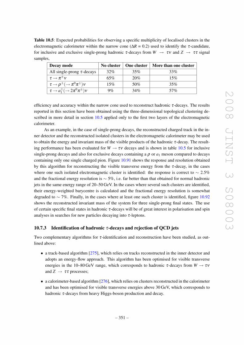
2008 JINST 3 S08003

Table 10.5: Expected probabilities for observing a specific multiplicity of localised clusters in theelectromagnetic calorimeter within the narrow cone (∆R = 0.2) used to identify the τ-candidate,for inclusive and exclusive single-prong hadronic τ-decays from W → τν and Z → ττ signalsamples,

Decay mode No cluster One cluster More than one clusterAll single-prong τ-decays 32% 35% 33%τ → π±ν 65% 20% 15%τ → ρ±(→ π0π±)ν 15% 50% 35%τ → a±1 (→ 2π0π±)ν 9% 34% 57%

efficiency and accuracy within the narrow cone used to reconstruct hadronic τ-decays. The resultsreported in this section have been obtained using the three-dimensional topological clustering de-scribed in more detail in section 10.5 applied only to the first two layers of the electromagneticcalorimeter.

As an example, in the case of single-prong decays, the reconstructed charged track in the in-ner detector and the reconstructed isolated clusters in the electromagnetic calorimeter may be usedto obtain the energy and invariant mass of the visible products of the hadronic τ-decay. The result-ing performance has been evaluated for W → τν decays and is shown in table 10.5 for inclusivesingle-prong decays and also for exclusive decays containing a ρ or a1 meson compared to decayscontaining only one single charged pion. Figure 10.91 shows the response and resolution obtainedby this algorithm for reconstructing the visible transverse energy from the τ-decay, in the caseswhere one such isolated electromagnetic cluster is identified: the response is correct to ∼ 2.5%and the fractional energy resolution is ∼ 5%, i.e. far better than that obtained for normal hadronicjets in the same energy range of 20–50 GeV. In the cases where several such clusters are identified,their energy-weighted barycentre is calculated and the fractional energy resolution is somewhatdegraded to ∼ 7%. Finally, in the cases where at least one such cluster is identified, figure 10.92shows the reconstructed invariant mass of the system for three single-prong final states. The useof certain specific final states in hadronic τ-decays will be of great interest in polarisation and spinanalyses in searches for new particles decaying into τ-leptons.

10.7.3 Identification of hadronic τ-decays and rejection of QCD jets

Two complementary algorithms for τ-identification and reconstruction have been studied, as out-lined above:

• a track-based algorithm [275], which relies on tracks reconstructed in the inner detector andadopts an energy-flow approach. This algorithm has been optimised for visible transverseenergies in the 10–80 GeV range, which corresponds to hadronic τ-decays from W → τν

and Z → ττ processes;

• a calorimeter-based algorithm [276], which relies on clusters reconstructed in the calorimeterand has been optimised for visible transverse energies above 30 GeV, which corresponds tohadronic τ-decays from heavy Higgs-boson production and decay.

– 351 –

2008 JINST 3 S08003

truth

)/Etruth

- Erec

(E-1 -0.8 -0.6 -0.4 -0.2 -0 0.2 0.4 0.6 0.8 1

Arb

itrar

y un

its

0

20

40

60

80

100

ν ρ → τ

0.2)% ± mean = - (2.4 0.2)% ± = (4.6 σ

Invariant mass (GeV)0 0.5 1 1.5 2 2.5

Arb

itrar

y un

its

0

50

100

150

200

250 ν ρ → τ

ν) π 0π 2 →(1 a→ τ ν π → τ

Figure 10.91: Energy response, expressedas the ratio (Erec − Etruth/Etruth, where Erec

(resp. Etruth) are the reconstructed (resp. true)visible energies (see text), for single-pronghadronic τ-decays from a W → τν signalsample with one reconstructed electromagneticcluster.

Figure 10.92: Distribution of reconstructedinvariant mass of visible decay products (seetext), for single-prong hadronic τ-decays froma W → τν signal sample with at least one re-constructed electromagnetic cluster.

Figures 10.93 and 10.94 show the expected performance of the two algorithms, expressedas curves describing jet rejection versus efficiency for single- and three-prong hadronic τ-decaysseparately and for different ranges of the visible transverse energy. The jet rejections are computedwith respect to truth jets reconstructed using particle four-momenta within a cone of size ∆R = 0.4.The behaviour of the respective rejection versus efficiency curves reflects the different optimisa-tions performed for the two algorithms. Whereas the track-based algorithm has been tuned topreserve similar performance for single- and three-prong decays, the calorimeter-based algorithmhas been tuned to provide the best possible rejection at medium-to-high energies and is thereforemore performant for single-prong decays than the track-based algorithm. For an overall efficiencyof 30% for single-prong decays, the rejection against jets is typically between 700 and 6000, as isillustrated more quantitatively and as a function of the visible transverse energy in table 10.6.

The track-based algorithm requires a good-quality track system, in which the leading trackhas transverse momentum above 9 GeV, as a seed for building a hadronic τ-candidate. This pro-vides already after reconstruction considerable rejection against QCD jets with high track multi-plicities. This is illustrated in figures 10.95 and 10.96, which show respectively the normalisedtrack-multiplicity spectra for hadronic τ-candidates, with visible transverse energy above 20 GeV,from Z → ττ decays and from QCD jets. The distributions are shown after the reconstruction step,after a cut-based identification algorithm and finally after applying a multi-variate discriminationtechnique using a neural network. The track multiplicity in the QCD jet sample is quite differentfrom that in the signal sample, for any of the cuts applied. At the same time, figure 10.95 shows thatthe fractions of single-prong and three-prong decays in the signal sample approach those expectedfrom an ideal signal sample: for single-prong (respectively three-prong) candidates, the fractionsof correctly assigned decays improve from 87% (respectively 74%) after reconstruction to 91%(respectively 86%) after cut-based identification and to 92% (respectively 93%) after applying theneural-network discrimination technique.

– 352 –

2008 JINST 3 S08003

Efficiency0 0.1 0.2 0.3 0.4 0.5 0.6 0.7 0.8 0.9 1

Rej

ectio

n

210

310

410

510 = 10 - 30 GeV

T 1-prong, E

= 30 - 60 GeVT

1-prong, E

= 10 - 30 GeVT

3-prong, E

= 30 - 60 GeVT

3-prong, E

Efficiency0 0.1 0.2 0.3 0.4 0.5 0.6 0.7 0.8 0.9 1

Rej

ectio

n

210

310

410

510

Efficiency0 0.1 0.2 0.3 0.4 0.5 0.6 0.7 0.8 0.9 1

Rej

ectio

n

210

310

410

510 = 60 - 100 GeV

T1-prong, E

> 100 GeVT

1-prong, E = 60 - 100 GeV

T3-prong, E

> 100 GeVT

3-prong, E

Figure 10.93: Expected rejection againsthadronic jets as a function of the efficiency forhadronic τ- decays for the track-based algo-rithm using a neural-network selection. Theresults are shown separately for single- andthree-prong decays and for two ranges of vis-ible transverse energy.

Figure 10.94: Expected rejection againsthadronic jets as a function of the efficiency forhadronic τ- decays for the calorimeter-based al-gorithm using a likelihood selection. The re-sults are shown separately for single- and three-prong decays and for two ranges of visibletransverse energy.

Track multiplicity0 1 2 3 4 5 6 7 8 9

Pro

babi

lity

0

0.1

0.2

0.3

0.4

0.5

0.6

0.7

0.8

0.9

1

Reconstruction

Identification with cuts

Identification with NN

τ τ → Z

> 20 GeV T E

Track multiplicity0 1 2 3 4 5 6 7 8 9

Pro

babi

lity

0

0.1

0.2

0.3

0.4

0.5

0.6

0.7

0.8

0.9

1

Reconstruction

Identification with cuts

Identification with NN

QCD jets

> 20 GeV T E

Figure 10.95: Track multiplicity distributionsobtained for hadronic τ-decays with visibletransverse energy above 20 GeV using thetrack-based τ-identification algorithm. Thedistributions are shown after reconstruction,after cut-based identification and finally afterapplying the neural network (NN) discrimina-tion technique for an efficiency of 30% for thesignal.

Figure 10.96: Track multiplicity distributionsobtained for the background from QCD jetswith visible transverse energy above 20 GeVusing the track-based τ-identification algo-rithm. The distributions are shown afterreconstruction, after cut-based identificationand finally after applying the neural network(NN) discrimination technique for an efficiencyof 30% for the signal.

– 353 –

2008 JINST 3 S08003

Table 10.6: Rejection of track-based and calorimeter-based τ-identification algorithms over therange of visible transverse energy in which they have been optimised. The values are given sep-arately for single- and three-prong decays and for an efficiency of 30%. The quoted errors arestatistical.

Algorithm ET = 10-30 GeV ET = 30-60 GeV ET = 60-100 GeV ET > 100 GeVTrack-based 1-prong 740±70 1030±160(neural network) 3-prong 590±50 590±70Calorimeter-based 1-prong 1130±50 2240±140 4370±280(likelihood) 3-prong 187±3 310±7 423±8

Figures 10.95 and 10.96 also show that the candidates with track multiplicity above three maybe used to normalise the QCD background. This would allow a reasonably precise calibration ofthe performance of the τ-identification algorithms using real data, provided the rejection againstQCD jets is proven to be sufficient to extract a clean signal in the single-prong and three-prongcategories. The sensitivity of such a method can be enhanced by also studying the track multi-plicity outside the narrow cone used for τ-identification and combining this information with thatpresented in figure 10.96.

10.8 Flavour tagging

The ability to tag hadronic jets arising from heavy flavours is an important asset for many physicsanalyses, such as precision measurements in the top-quark sector and searches for Higgs bosonsor other new physics signatures. This section describes the b-tagging performance which can beachieved using different methods [277]. In the results presented in this section, the impact ofpossible residual misalignements on the b-tagging performance has not been taken into account.

10.8.1 Ingredients of b-tagging algorithms

Except when explicitly stated otherwise, the results presented in this section are based on simula-tions without pile-up and with a perfect alignment of the inner detector. Jets are reconstructed inthe calorimeters using standard algorithms (see section 10.5.1) and the jets with pT > 15 GeV and|η |< 2.5 are considered for b-tagging. Only reconstructed tracks within a distance ∆R < 0.4 fromthe jet axis are used for b-tagging.

To assess quantitatively the b-tagging performance, the Monte-Carlo truth is used to deter-mine the type of parton from which a jet originates. This labelling procedure is somewhat ambigu-ous. For the results presented here, a quark-based labelling has been used: a jet is labelled as a b-jetif a b-quark with pT > 5 GeV is found in a cone of size ∆R = 0.3 around the jet direction. A jet islabelled as a c-jet (or τ-jet) if a c-quark (or τ-lepton) with pT > 5 GeV is found in the cone insteadof a b-quark. When no heavy quark nor τ-lepton satisfies these requirements, the jet is labelled asa light jet. No attempt is made to distinguish between u-, d-, s-quarks and gluons. It is importantto note that this labelling procedure defines as b-jets most gluon jets splitting to a bb pair in theparton-shower process.

– 354 –

2008 JINST 3 S08003

Signed transverse impact parameter (mm)-1 -0.8 -0.6 -0.4 -0.2 -0 0.2 0.4 0.6 0.8 1

Arb

itrar

y un

its

-410

-310

-210

-110 Tracks in b-jets

Tracks in c-jets

Tracks in light jets

Signed transverse impact parameter significance-20 -10 0 10 20 30 40

Arb

itrar

y un

its

-610

-510

-410

-310

-210

-110 Tracks in b-jets

Tracks in c-jets

Tracks in light jets

Figure 10.97: Signed transverse impact param-eter, d0, distribution for b-jets, c-jets and lightjets.

Figure 10.98: Signed transverse impact param-eter significance, d0/σd0 , distribution for b-jets,c-jets and light jets.

10.8.1.1 Track selection and track impact parameters

The track selection for b-tagging is designed to select well-measured tracks and to reject faketracks in jets and secondary tracks from K0

s , Λ and hyperon decays, as well as electrons fromphoton conversions. Only tracks with transverse momentum above 1 GeV are considered. At leastseven precision hits (pixels and strips) are required, of which at least two must be in the pixeldetector and one in the pixel vertexing layer. The transverse (d0) and longitudinal (z0) impactparameters at the point of closest approach to the vertex must fulfil respectively, |d0| < 1 mm and|z0− zv|sinθ < 1.5 mm, where zv is the reconstructed primary vertex position in z and θ is themeasured polar angle of the track. The efficiency of these cuts and the resulting fake-track rate injets are discussed in section 10.2.3 (see in particular figure 10.14).

For the b-tagging algorithms, the impact parameters of tracks are computed with respect tothe primary vertex (see section 10.2.4). The transverse impact parameter is signed using the jetdirection as measured by the calorimeters: tracks crossing the jet axis behind the primary vertexhave a negative impact parameter. The distribution of the signed transverse impact parameter, d0,is shown in figure 10.97 for tracks reconstructed in b-jets, c-jets and light jets. Figure 10.98 showsthe corresponding significance distribution, d0/σd0 , which gives more weight to precisely measuredtracks.

10.8.1.2 Secondary vertices

To further increase the discrimination between b-jets and light jets, the inclusive vertex formedby the decay products of the B-hadron, including the products of the subsequent charm hadrondecay, can be reconstructed. The search starts by combining all track pairs which form a goodvertex, using only tracks with a high impact-parameter significance in order to remove the trackswhich are compatible with the primary vertex. The invariant mass of the particles originating from

– 355 –

2008 JINST 3 S08003

Secondary vertex mass (GeV)0 1 2 3 4 5 6 7 8 9 10

Arb

itrar

y un

its

-410

-310

-210

-110 b-jets

Light jets

Secondary vertex charged energy fraction0 0.1 0.2 0.3 0.4 0.5 0.6 0.7 0.8 0.9 1

Arb

itrar

y un

its

-310

-210

b-jetsLight jets

Number of two-track vertices0 5 10 15 20 25 30

Arb

itrar

y un

its

-510

-410

-310

-210

-110

1b-jets

Light jets

Figure 10.99: Properties of secondary vertices reconstructed in b-jets and light jets: invariant massof all tracks originating from the vertex (left), the ratio of the sum of the energies of the tracksoriginating from the vertex to the sum of the energies of all tracks in the jet (middle) and numberof two-track vertices (right).

the secondary vertex candidate and the location of this vertex candidate are used to reject verticeswhich are likely to come from K0

s /Λ decays and photon conversions or from secondary interactionsin material such as the beam-pipe or the vertexing layer. All tracks from the remaining two-trackvertices are combined into a single vertex and three of its properties are exploited: the invariantmass of all the tracks originating from the vertex, the ratio of the sum of the energies of the tracksoriginating from the vertex to the sum of the energies of all tracks in the jet, and the number oftwo-track vertices. These properties are illustrated in figure 10.99 for b-jets and light jets. Thesecondary-vertex reconstruction efficiency depends quite strongly on the event topology and thetypical efficiencies achieved are higher than 60% for the tt and WH events studied here.

10.8.2 Likelihood-ratio tagging algorithms

For both the impact-parameter tagging and the secondary-vertex tagging, a likelihood-ratio methodis used: the discriminating variables are compared to pre-defined smoothed and normalised distri-butions for both the b- (signal) and light- (background) jet hypotheses. Multi-dimensional probabil-ity density functions are used as well for some b-tagging algorithms. The ratio of the probabilitiesdefines the track or vertex weight, which can be combined in a jet weight as the sum of the log-arithms of the individual weights. The distribution of such a weight is shown in figures 10.100and 10.101 for b-, c- and light jets for two different b-tagging algorithms: the first one combinesonly the transverse impact parameter significance of tracks, while the second one combines in twodimensions the transverse and longitudinal impact parameter significances of tracks as well as thethree variables from the secondary vertex search discussed above. The former algorithm is simplerand more robust than the latter which will require more time to commission. Currently, no use ismade of probability density functions for c-jets, and these are not considered when creating thereference distributions for the signal and background hypotheses.

– 356 –

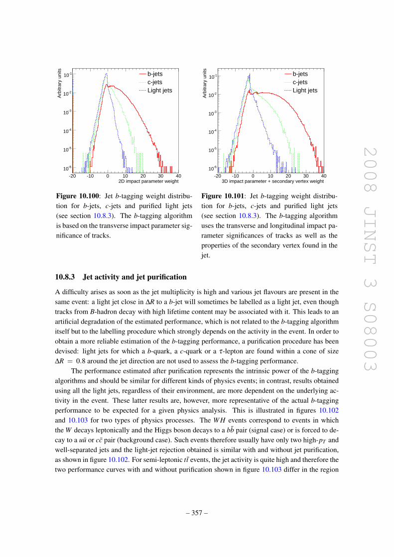
2008 JINST 3 S08003

2D impact parameter weight-20 -10 0 10 20 30 40

Arb

itrar

y un

its

-610

-510

-410

-310

-210

-110 b-jetsc-jetsLight jets

3D impact parameter + secondary vertex weight-20 -10 0 10 20 30 40

Arb

itrar

y un

its

-610

-510

-410

-310

-210

-110 b-jetsc-jetsLight jets

Figure 10.100: Jet b-tagging weight distribu-tion for b-jets, c-jets and purified light jets(see section 10.8.3). The b-tagging algorithmis based on the transverse impact parameter sig-nificance of tracks.

Figure 10.101: Jet b-tagging weight distribu-tion for b-jets, c-jets and purified light jets(see section 10.8.3). The b-tagging algorithmuses the transverse and longitudinal impact pa-rameter significances of tracks as well as theproperties of the secondary vertex found in thejet.

10.8.3 Jet activity and jet purification

A difficulty arises as soon as the jet multiplicity is high and various jet flavours are present in thesame event: a light jet close in ∆R to a b-jet will sometimes be labelled as a light jet, even thoughtracks from B-hadron decay with high lifetime content may be associated with it. This leads to anartificial degradation of the estimated performance, which is not related to the b-tagging algorithmitself but to the labelling procedure which strongly depends on the activity in the event. In order toobtain a more reliable estimation of the b-tagging performance, a purification procedure has beendevised: light jets for which a b-quark, a c-quark or a τ-lepton are found within a cone of size∆R = 0.8 around the jet direction are not used to assess the b-tagging performance.

The performance estimated after purification represents the intrinsic power of the b-taggingalgorithms and should be similar for different kinds of physics events; in contrast, results obtainedusing all the light jets, regardless of their environment, are more dependent on the underlying ac-tivity in the event. These latter results are, however, more representative of the actual b-taggingperformance to be expected for a given physics analysis. This is illustrated in figures 10.102and 10.103 for two types of physics processes. The WH events correspond to events in whichthe W decays leptonically and the Higgs boson decays to a bb pair (signal case) or is forced to de-cay to a uu or cc pair (background case). Such events therefore usually have only two high-pT andwell-separated jets and the light-jet rejection obtained is similar with and without jet purification,as shown in figure 10.102. For semi-leptonic tt events, the jet activity is quite high and therefore thetwo performance curves with and without purification shown in figure 10.103 differ in the region

– 357 –

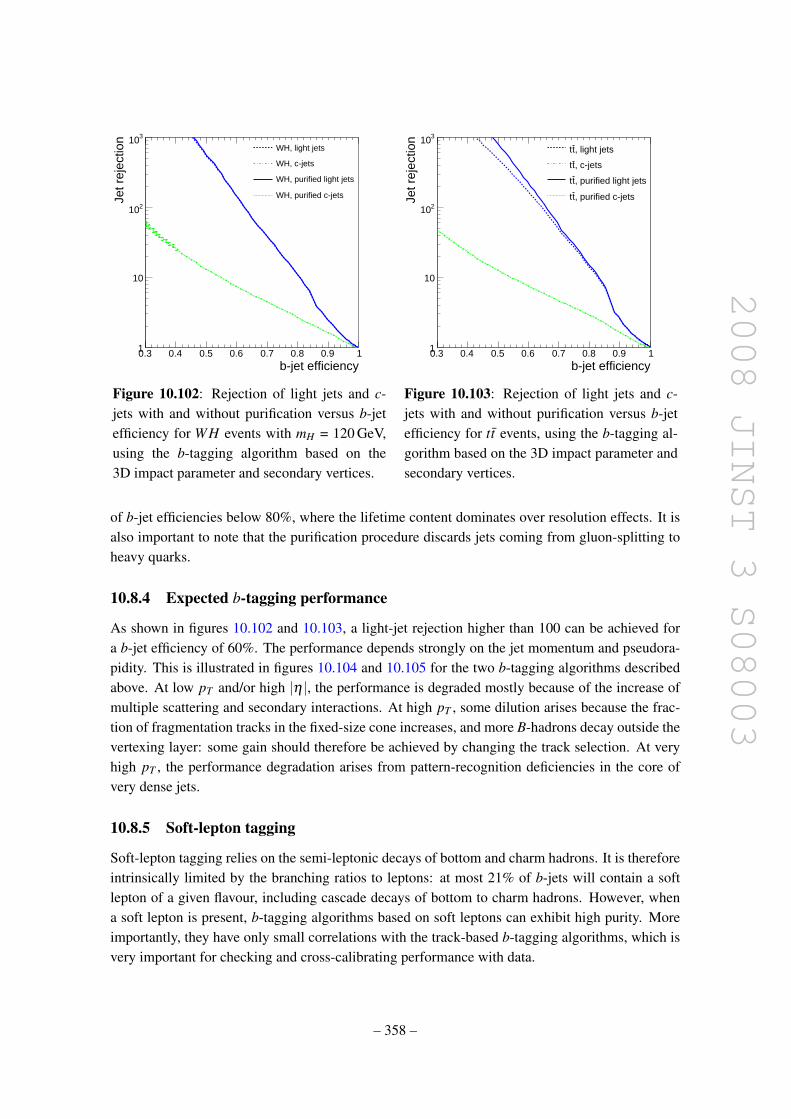
2008 JINST 3 S08003

b-jet efficiency0.3 0.4 0.5 0.6 0.7 0.8 0.9 1

Jet r

ejec

tion

1

10

210

310WH, light jets

WH, c-jets

WH, purified light jets

WH, purified c-jets

b-jet efficiency0.3 0.4 0.5 0.6 0.7 0.8 0.9 1

Jet r

ejec

tion

1

10

210

310, light jetstt

, c-jetstt

, purified light jetstt

, purified c-jetstt

Figure 10.102: Rejection of light jets and c-jets with and without purification versus b-jetefficiency for WH events with mH = 120 GeV,using the b-tagging algorithm based on the3D impact parameter and secondary vertices.

Figure 10.103: Rejection of light jets and c-jets with and without purification versus b-jetefficiency for tt events, using the b-tagging al-gorithm based on the 3D impact parameter andsecondary vertices.

of b-jet efficiencies below 80%, where the lifetime content dominates over resolution effects. It isalso important to note that the purification procedure discards jets coming from gluon-splitting toheavy quarks.

10.8.4 Expected b-tagging performance

As shown in figures 10.102 and 10.103, a light-jet rejection higher than 100 can be achieved fora b-jet efficiency of 60%. The performance depends strongly on the jet momentum and pseudora-pidity. This is illustrated in figures 10.104 and 10.105 for the two b-tagging algorithms describedabove. At low pT and/or high |η |, the performance is degraded mostly because of the increase ofmultiple scattering and secondary interactions. At high pT , some dilution arises because the frac-tion of fragmentation tracks in the fixed-size cone increases, and more B-hadrons decay outside thevertexing layer: some gain should therefore be achieved by changing the track selection. At veryhigh pT , the performance degradation arises from pattern-recognition deficiencies in the core ofvery dense jets.

10.8.5 Soft-lepton tagging

Soft-lepton tagging relies on the semi-leptonic decays of bottom and charm hadrons. It is thereforeintrinsically limited by the branching ratios to leptons: at most 21% of b-jets will contain a softlepton of a given flavour, including cascade decays of bottom to charm hadrons. However, whena soft lepton is present, b-tagging algorithms based on soft leptons can exhibit high purity. Moreimportantly, they have only small correlations with the track-based b-tagging algorithms, which isvery important for checking and cross-calibrating performance with data.

– 358 –

2008 JINST 3 S08003

(GeV)T

p0 50 100 150 200 250 300

Ligh

t-je

t rej

ectio

n

0

50

100

150

200

250

300

350

4003D impact parameter + secondary vertex

2D impact parameter

|η|0 0.5 1 1.5 2 2.5

Ligh

t-je

t rej

ectio

n

0

50

100

150

200

250

300

350

400

4503D impact parameter + secondary vertex

2D impact parameter

Figure 10.104: Rejection of purified light jetsas a function of the jet transverse momentumfor two different b-tagging algorithms operat-ing at a fixed b-tagging efficiency of 60% ineach bin.

Figure 10.105: Rejection of purified light jetsas a function of the jet pseudorapidity for twodifferent b-tagging algorithms operating at afixed b-tagging efficiency of 60% in each bin.

Soft muons are reconstructed using two complementary reconstruction algorithms (see sec-tion 10.3): combined muons, which correspond to a track fully reconstructed in the muon spec-trometer and matched with a track in the inner detector, and muons with a low momentum, typ-ically below ∼ 5 GeV, which cannot reach the muon middle and outer stations and are identi-fied by matching an inner-detector track with a segment in the muon spectrometer inner stationsonly. Muons reconstructed in this way and satisfying some basic selection criteria, pT > 4 GeVand |d0| < 4 mm, are associated to the closest jet provided their distance to the jet axis satisfies∆R < 0.5. Finally, the kinematic properties of the jet-muon system, such as the relative transversemomentum of the muon with respect to the jet axis, are used in order to reject the backgroundcaused by punch-through particles and decays in flight in light jets. As shown in figure 10.106for tt events, the soft-muon b-tagging algorithm yields an efficiency of 10% (including branchingratios and identification efficiency) and a light-jet rejection of 200 for jets with pT > 15 GeV and|η | < 2.5. The rejection against light jets decreases by approximately 30% when the expectedcontributions from pile-up and especially cavern background at 1033 cm−2 s−1 are included.

Reconstructing soft electrons in jets in the electromagnetic calorimeter is more difficult be-cause of the overlap of hadronic showers with the electron shower itself. This is achieved using thesoft-electron algorithm [266] which matches an inner-detector track to an electromagnetic cluster,as described in section 10.4.1. The performance of this algorithm is, however, highly dependenton the track density in the jets as well as on the amount of material in front of the electromagneticcalorimeter (photon conversions). As shown in figure 10.107, a light-jet rejection of 90 can beachieved for an efficiency of 7% in WH events. Currently, for a 7% (respectively 10%) b-taggingefficiency, about 75% (respectively 40%) of the surviving light jets are tagged by electrons orig-inating from photon conversions: the performance would therefore substantially improve if theseconversions could be rejected further.

– 359 –

2008 JINST 3 S08003

b-jet efficiency0.07 0.08 0.09 0.1 0.11 0.12 0.13

Ligh

t-je

t rej

ectio

n

210

310

tt

with pile-up and cavern backgroundtt

b-jet efficiency0.04 0.06 0.08 0.1 0.12 0.14

Ligh

t-je

t rej

ectio

n

210

310

Figure 10.106: Rejection of light jets versus b-tagging efficiency in tt events (branching ratiosto lepton and lepton identification efficiency in-cluded) for the soft-muon b-tagging algorithm.The results are shown without and with the pile-up and cavern background expected at a lumi-nosity of 1033 cm−2 s−1.

Figure 10.107: Rejection of light jets versusb-tagging efficiency in WH events (branchingratios to lepton and lepton identification effi-ciency included) for the soft-electron b-taggingalgorithm.

10.9 Trigger performance

10.9.1 Overview

This section gives an overview of the performance achieved on simulated raw data using the onlinephysics selection strategy of ATLAS. As already mentioned in section 8.1, components of thereconstruction and analysis software, implemented mostly in the offline environment in previousexperiments, have had to be embedded within the trigger system to achieve the required rejectionpower while retaining excellent sensitivity to the various physics signatures of interest. A greatdeal of flexibility is provided by the three-level trigger system to adapt to changes in the luminosity(from fill-to-fill and even during a single fill), to variations in the background conditions, and to newrequirements which will undoubtedly arise as the understanding of the physics, trigger performanceand detector develops.

The approach taken to guarantee good acceptance for as broad a spectrum of physics aspossible is to use mainly inclusive criteria for the online selection, i.e. signatures mostly based onsingle- and di-object high-pT triggers. The choice of the thresholds is made to have a good overlapwith the reach of the Tevatron and other colliders, and to ensure good sensitivity to new particlesover a wide range of masses and decay channels. This high-pT inclusive selection is complementedwhere necessary with more focussed signatures, such as the presence of several different physicsobjects or the use of topological criteria.

10.9.2 Selection strategy

The architecture of the trigger and data acquisition system is described in section 8.3 (see in partic-ular figure 8.1) and is based on a three-level trigger system, with a first level (L1) using hardwarebased on ASIC’s and FPGA’s, and the other two (L2 and EF or event filter, collectively also called

– 360 –

2008 JINST 3 S08003

high-level triggers or HLT) using software algorithms running on farms of commercial computers.At L2, the event selection is based on specialised algorithms, optimised for speed, whereas theEF uses more complex algorithms, basically identical to those used in the offline reconstructionsoftware.

The L2 and EF algorithms are usually "seeded", meaning that reconstruction is normallyguided by the previous trigger level to access and process data only in a "Region-of-Interest" (RoI)containing particle candidates. This significantly reduces the processing time (and also data move-ment from the holding buffers to the L2 processors), without degrading the selection performance.For the EF, and even for L2 where necessary, data can be accessed and processed from the fulldetector, within the constraints of available data-movement and processing resources. This appliesfor example to scans of the complete inner detector for low-pT tracks for the B-physics selection orto the processing of all calorimeter cells for an improved calculation of missing transverse energy.At L2, this can only be done in special cases and for a small fraction of the events due to bandwidthlimitations, whereas in the EF the full event data are available in memory. It is also possible to useso-called secondary RoI’s which did not contribute to the L1 selection, but provide the coordinatesof lower-pT objects which can be included in the L2 selection.

In the HLT, "feature-extraction" algorithms are used to identify objects (such as electrons orjets) and determine their properties or to determine global characteristics of the event. The sequenceof execution of the algorithms (e.g. ordered according to complexity) is chosen to maximise thephysics potential and retain adequate flexibility within the available data-movement and processingresources of the HLT. After each step in the sequence, hypothesis algorithms determine whethera given signature is satisfied or not. The processing of any given RoI is stopped as soon as it isclear that it cannot contribute to the selection of the event. The event itself is rejected if none of thesignatures in the trigger menu is satisfied.

The initial implementation and capabilities of the DAQ/HLT system are described in sec-tion 8.4, where it is stated that the system should handle a L1 trigger rate of ∼ 40 kHz, i.e. approx-imately 50% of the design specification. Clearly, only the availability of real data will allow thewhole strategy to be finalised. However, it is important to be able to face this initial phase with themost complete set of tools possible and with a versatile selection architecture, in order to cope withthe surprises which are likely to appear at the time of LHC start-up.

10.9.3 Trigger menus

Trigger menus are tables which specify thresholds and selection criteria at each of the three trig-ger levels to address the physics-analysis requirements of ATLAS. The process of preparing themenus takes into account an assessment of the rejection capabilities at each selection stage and foreach signature, and the rate capabilities of each level of the trigger and of the offline computingsystem. This procedure is iterative and makes use of earlier studies of the L1 trigger and HLT, asdocumented in [204, 237].

Trigger items, defined as entries in the trigger menu corresponding to selected physics ob-jects, are identified using a notation where a symbol representing a particle type is preceded bya multiplicity value and followed by a ET -threshold value, e.g. 2e5 corresponds to a requirementof two or more electrons, each with ET above 5 GeV. The threshold value quoted for L1 is the

– 361 –

2008 JINST 3 S08003

Table 10.7: Subset of items from an illustrative trigger menu at 1031 cm−2 s−1.

Signature L1 rate (Hz) HLT rate (Hz) CommentsMinimum bias Up to 10000 10 Pre-scaled trigger item

e10 5000 21 b,c→ e, W , Z, Drell-Yan, tt2e5 6500 6 Drell-Yan, J/ψ , ϒ, Zγ20 370 6 Direct photons, γ-jet balance2γ15 100 < 1 Photon pairsµ10 360 19 W , Z, tt2µ4 70 3 B-physics, Drell-Yan, J/ψ , ϒ, Z

µ4 + J/ψ(µµ) 1800 < 1 B-physicsj120 9 9 QCD and other high-pT jet final states4j23 8 5 Multi-jet final states

τ20i + xE30 5000 (see text) 10 W , ttτ20i + e10 130 1 Z→ ττ

τ20i + µ6 20 3 Z→ ττ

raw ET cut applied in the hardware, and high efficiency is only achieved for particles or jets ofsomewhat higher ET ; this differs from the definition used in previous documents [237]. For in-clusive selections, the multiplicity requirement of one is implicit. An "i" following the thresholdindicates that an isolation requirement is made in addition. For example, τ20i requires at least onehadronic τ candidate with transverse energy above 20 GeV and with a specific calorimeter isolationrequirement in addition. The term "xE" is a short form for Emiss

T .The steering and configuration of the trigger (see section 8.3.6) support the description of

both straightforward RoI-based triggers like single electrons, muons, τ-leptons and jets along withmore complex triggers like Emiss

T and triggers for B-physics. For each trigger level, items in themenu can be pre-scaled to reduce their rates, or "pass-through" flags can be raised, where eventsare accepted irrespective of the HLT selection decision for the purpose of systematic studies.

The initial start-up luminosity at the LHC is expected to be around 1031 cm−2 s−1. This pro-vides convenient conditions for commissioning the trigger and the detector sub-systems, validatingthe trigger and offline software algorithms, and ensuring that basic Standard Model signatures canbe observed. The trigger menu for this start-up scenario reflects these requirements and allows forlow pT -thresholds on final-state leptons and photons, without any pre-scaling at L1, and for higherpT -thresholds, for which most of the HLT algorithms are executed in "pass-through" mode.

Table 10.7 presents an example of a sample of the triggers which will be used at start-up. Therates shown have been estimated using non-diffractive minimum-bias events with a total assumedcross-section of 70 mb. Triggering on single and di-leptons should be possible with quite low pT -thresholds and without applying isolation or other complex criteria, which must be validated withreal data at turn-on. With the exception of the minimum-bias selection, the items indicated arethose which should be operable without pre-scaling at 1031 cm−2 s−1. The full menu contains anumber of additional components, including many pre-scaled items with lower thresholds.

– 362 –

2008 JINST 3 S08003

The rates for combined triggers which require two or more final-state leptons or photons areexpected to be low in most instances, allowing them to be run without pre-scaling with very lowthresholds. Significant bandwidth will be devoted to collecting large samples of minimum-biasdata for use in physics analysis and for detector and trigger performance studies. Multi-jet trig-gers will be run at a comparatively high rate to test b-jet tagging in the HLT which is discussedin section 10.9.6. A small amount of bandwidth is allocated for inclusive Emiss

T and scalar sum-ET triggers, as well as using the Emiss

T signature in combination with other criteria. Note that forthe item τ20i + xE30 in table 10.7, the Emiss

T selection is made only at the EF level, in case thecorresponding L1 selection takes time to commission. The rate of the τ20i item at L1 is approxi-mately 5 kHz.

The quoted trigger rates are subject to large uncertainties on the cross-sections for QCD pro-cesses in proton-proton collisions at LHC energies, and on the modelling of the performance ofthe detector. The rates indicated assume that the selection cuts will already have been reasonablywell tuned to achieve high background rejection with good signal efficiency. There is still scopeto use tighter cuts and more delicate variables such as isolation after extensive optimisation andthorough validation. Should the rates turn out to be higher than estimated, the inclusive thresholdscould be raised substantially without compromising much of the main initial physics programme,but nevertheless to the detriment of an efficient collection of large data samples required for theinitial understanding of the detector performance.

10.9.4 Examples of trigger performance

The expected trigger performance at an initial luminosity of 1031 cm−2 s−1 is illustrated in the fol-lowing with representative examples from the menu discussed above. As documented in ref. [237]and discussed briefly in section 10.9.6, the trigger also meets the physics requirements up to aluminosity of 1034 cm−2 s−1.

The performance results presented here were obtained using an exact simulation of the al-gorithms which are implemented in the L1 hardware and using the same HLT algorithms as thosewhich are run online. The full HLT chain was used to obtain the performance results. As de-scribed in section 10.1, these studies have also been made for data simulated with a misaligned andmis-calibrated detector to verify, and improve if necessary, the robustness of the selection.

10.9.4.1 Electrons and photons

The performance of the electron and photon triggers has been evaluated for a luminosityof 1031 cm−2 s−1, using simulations of single particles and selected physics channels. The trig-ger efficiencies are quoted with respect to events containing electrons and photons identified withloose offline particle identification cuts (see section 10.4). Inefficiency in the trigger selection arisesmainly from tighter selection requirements needed to reduce the background rate to an acceptablelevel. There are also small losses due to the coarser calorimeter granularity used at L1 and thesimpler (and faster) selection algorithms applied at L2 compared to the offline reconstruction.

Figure 10.108 shows the L1, L2 and EF efficiencies as a function of ET for the signature e10,the menu item selecting electrons with ET > 10 GeV, as estimated using simulations of singleelectrons. The efficiency reaches a plateau value for ET above ∼ 15 GeV and is quite uniform as afunction of |η |, except for a 10–20% dip in the transition region between the barrel and the end-cap

– 363 –

2008 JINST 3 S08003

(GeV)TE0 5 10 15 20 25 30 35 40

Trig

ger

effic

ienc

y

0

0.2

0.4

0.6

0.8

1

L1L2EF

|η|0 0.5 1 1.5 2 2.5

Nor

mal

ised

rat

e

0

0.1

0.2

0.3

0.4

0.5

0.6

0.7

L1

L2

EF

Figure 10.108: Trigger efficiencies at L1, L2and EF as a function of the true electron ET

for the e10 menu item. The efficiencies are ob-tained for single electrons and are normalisedwith respect to the medium set of offline elec-tron cuts discussed in section 10.4.

Figure 10.109: Relative rates versus |η | for jetspassing the L1, L2 and EF trigger selections forthe e10 menu item. The relative rates are shownfor each of the seven η- ranges used to opti-mise the offline selection of isolated electronsand are normalised as described in the text.

(GeV)TE0 5 10 15 20 25 30 35 40

Trig

ger

effic

ienc

y

0

0.2

0.4

0.6

0.8

1

L1L2EF

|η|0 0.5 1 1.5 2 2.5

Nor

mal

ised

rat

e

0

0.1

0.2

0.3

0.4

0.5

0.6

0.7

L1

L2

EF

Figure 10.110: Trigger efficiencies at L1, L2and EF as a function of the true photon ET forthe γ20i menu item. The efficiencies are ob-tained for single photons and normalised withrespect to loose offline photon identificationcuts.

Figure 10.111: Normalised relative rates ver-sus |η | for jets passing the L1, L2 and EF trig-ger selections for the γ20i menu item. The rela-tive rates are shown for each of the six η-rangesused to optimise the offline selection of isolatedphotons and are normalised as described in thetext. The bin corresponding to the barrel/end-cap transition region is not shown because theoffline selection excludes it.

calorimeters. Figure 10.109 shows the normalised relative rates expected from QCD jets satisfyingthe e10 signature as a function of |η | for the successive trigger levels. These relative rates arenormalised for each trigger level to the total number of events selected and then the rate in each binis rescaled to that expected for a bin of fixed size ∆η = 0.5. The rates are quite sensitive to the resultof the trigger efficiency optimisation and their non-uniformity reflects the lower efficiency in theregions where the electromagnetic calorimeter performance is not optimal, as in the barrel/end-captransition region with 1.37 < |η | < 1.52. Similar results are obtained for photons and shown forthe signature γ20i, the menu item selecting isolated photons with ET > 20 GeV, in figures 10.110and 10.111.

– 364 –

2008 JINST 3 S08003

(GeV)TTrue Visible E0 20 40 60 80 100 120

Eff

icie

ncy

0

0.2

0.4

0.6

0.8

1

L1

L2

EF

(GeV)TTrue visible E0 20 40 60 80 100 120

Eff

icie

ncy

0

0.1

0.2

0.3

0.4

0.5

0.6

0.7

0.8

0.9

20iτ25iτ

35iτ

45iτ60iτ

Figure 10.112: Trigger efficiencies at L1, L2and EF as a function of the true visible ET ofthe hadronic τ-decays for the τ20i menu item.

Figure 10.113: Efficiency after EF for τ-triggeritems with different thresholds as a function ofthe true visible ET of the hadronic τ-decay.

10.9.4.2 τ-leptons and EmissT

The performance of the trigger for selecting high-pT τ-leptons is illustrated with the τ20i sig-nature selecting hadronic τ-decays with true visible ET of the hadronic τ-decay (defined as thesummed transverse energy of all the decay products which are not neutrinos) larger than 20 GeV.Figure 10.112 shows the trigger efficiency after each trigger level, normalised to an offline selec-tion with loose requirements (see section 10.7), for hadronic τ-decays from W → τν and Z → ττ

decays. The efficiency exhibits a drop of approximately 15% after L2, mostly because of theτ-identification cuts applied. The efficiency turn-on rises more slowly than for the electron andphoton triggers, especially at L1, reflecting the poorer resolution obtained for hadronic showers.Figure 10.113 shows the efficiency turn-on curves for various τ-trigger thresholds as a functionof the true visible ET of the hadronic τ-decay. The overall efficiency with respect to the offlineselection is typically 85% on the plateau.

A somewhat special case is that of EmissT triggers which can be used either inclusively or in

combination with other objects, in particular with jets or hadronic τ-triggers. Because EmissT is a

global property of the event, the RoI-driven L2 trigger is not capable of substantially improvingthe L1 trigger. However, the Emiss

T algorithm in the EF improves substantially on L1 by accessingthe precision readout of the entire calorimeter and performing a simplified version of the offlinealgorithm.

A challenging goal of the τ-selection during the low-luminosity period is to collect a largesample of W → τν decays. This can be achieved using a τ-trigger in combination with a require-ment (potentially only at the level of the EF) of substantial Emiss

T (see table 10.7). Such events areobviously interesting for physics analyses, but are also needed to monitor the hadronic energy scaleusing single charged pions, and for other performance studies. An additional goal is to providetriggers with low pT -thresholds and loose trigger requirements, in addition to the single high-pT

electron and muon triggers, for collecting efficiently Z-bosons decaying into two τ-leptons, whereone τ-lepton decays to an electron or muon and the other to hadrons. The background rates forthese e/µ+τ triggers are estimated to be in the range of one Hz or less at the initial luminosityof 1031 cm−2 s−1, with rather loose HLT cuts applied to the trigger objects.

– 365 –

2008 JINST 3 S08003

Table 10.8: Summary of L1 single-jet and multi-jet menu items, of L1 pre-scale factors and ex-pected L1 and EF rates at a luminosity of 1031 cm−2 s−1.

Trigger item j10 j18 j23 j35 j42 j70 j120 3j10 3j18 4j10 4j18 4j23Pre-scale factor at L1 42000 6000 2000 500 100 15 1 150 1 30 1 1L1 rate (Hz) 4 1 1 1 4 4 9 40 140 40 20 8EF rate (Hz) 4 1 1 1 4 4 9 0.05 1 0.04 0.1 5

10.9.4.3 Jets

The inclusive jet trigger j120 presented in table 10.7 is complemented by a series of pre-scaleditems chosen to give an approximately uniform rate across the jet ET -spectrum. Collecting suffi-cient statistics over the entire jet ET -spectrum is important for differential cross-section measure-ments and also for the measurement of detector, trigger and physics algorithm efficiencies. The setof threshold and pre-scale combinations is expected to be stable with rising luminosity for the firstfew years of data-taking. The strategy adopted to optimise the jet trigger menu for different lumi-nosities is then primarily to modify the pre-scale factors associated with each jet-trigger threshold,rather than to change the set of thresholds on an ad-hoc basis.

Table 10.8 summarises a set of L1 jet-trigger items, L1 pre-scale factors and L1 and EF ratesfor a luminosity of 1031 cm−2 s−1. Since the jet rates cannot be reduced much by the HLT, theEF rates quoted in table 10.8 are obtained through additional pre-scale factors applied wherevernecessary. Figure 10.114 shows the corresponding reconstructed differential ET spectrum of theleading jet after the L1 trigger accept. The differential distribution thus obtained is almost uniformover the range of L1 single-jet triggers run with different pre-scale factors, yielding about 108 lead-ing jets with ET in the range between 10 and 100 GeV for an integrated luminosity of 100 pb−1.Figure 10.115 shows that over this range of jet ET , the efficiency at threshold of the various pre-scaled jet trigger menu items turns on much more slowly than the corresponding curves for leptonsbecause of the poorer resolution of the jet ET reconstructed at L1.

10.9.4.4 Muons

The geometrical coverage of the muon trigger detector system (see section 6.6 for a detailed de-scription) limits the overall acceptance for triggering on muons at L1, as illustrated in figure 10.116.The barrel trigger system covers approximately 80% of the η-φ plane (over |η | < 1.0), while theend-cap trigger extends over approximately 96% of the relevant η-φ space. The limitations of thebarrel system can be seen in figure 10.116, and are dominated by the crack at η < 0.1 (largely toaccommodate inner-detector and calorimeter services), by the regions occupied by the feet of theexperiment and by the space taken by the barrel toroid ribs. The end-cap trigger coverage is limitedonly by the detector supports and by the holes needed for the optical alignment system. Within thefiducial acceptance of the trigger detectors, the L1 trigger efficiency for muons with pT larger thanthe selection thresholds exceeds 99%. The L2 trigger then provides a first reduction of the L1 ratesby confirming the muon candidates with a more precise measurement of their momentum and bymatching them to inner-detector tracks.

– 366 –

2008 JINST 3 S08003

of leading jet (GeV)TE10 210 310

)-1

(G

eVT

dN /

dE

-110

110

210

310

410

510

610

710

810

910

1010

1110

(GeV)TTrue E0 50 100 150 200 250

Effi

cien

cy

0

0.2

0.4

0.6

0.8

1

J10

J18

J23

J35

J42

J70

J120

Figure 10.114: Expected differential spec-trum for single jets as a function of the re-constructed ET of the leading jet. The solidline shows the distribution after applying theL1 trigger thresholds and pre-scale factors pre-sented in table 10.8, while the dashed line rep-resents the distribution expected without anytrigger requirements.

Figure 10.115: Efficiency as a function ofthe true jet ET (as defined for a cone ofsize ∆R = 0.4) for each of the single-jet L1menu items shown in table 10.8.

η-2 -1 0 1 2

(ra

dian

s)ϕ

-3

-2

-1

0

1

2

3

threshold (GeV)T

Muon p3 4 5 6 7 8 9 10 20 30 40

Rat

e (H

z)

-310

-210

-110

1

10

210

310CharmBeauty/K decaysπ

WTotal

Figure 10.116: Acceptance map in η-φ spacefor the L1 muon trigger, which covers the η-range |η | < 2.4. The black points representregions not instrumented with L1 trigger detec-tors because of the presence of various supportsand services.

Figure 10.117: Estimated EF output rates formuons as a function of pT -threshold at a lumi-nosity of 1031 cm−2 s−1, integrated over the fullη-range covered by the L1 trigger, |η | < 2.4.

The rates of muons at the output of the EF have been computed at a luminosity of1031 cm−2 s−1, by summing the contributions from the barrel and end-cap regions of the muonspectrometer. As shown in figure 10.117, several physics processes contribute significantly to therate. The rates given as a function of the pT -threshold are for an inclusive muon selection, withoutapplying an isolation requirement. The largest contributions to the total rate in the pT -range from 4to 6 GeV are from charm, beauty and in-flight decays of charged pions and kaons. Isolation, as wellas refined matching requirements between the tracks in the inner detector and muon spectrometer,can be used to further reduce the rates.

– 367 –

2008 JINST 3 S08003

10.9.4.5 B-physics

The trigger for B-physics is initiated by a single- or di-muon selection at L1. At 1031 cm−2 s−1,a threshold pT > 4 GeV will be used, rising to about 6 GeV at 1033 cm−2 s−1 to match the ratecapabilities of the HLT.

Figure 10.118: Trigger efficiency forBs → D−s a+

1 events passing the offline se-lection as a function of the pT of the B-meson.The results are shown for two HLT scenarios,the most performant one, based on a full scanof the inner detector which can be used at lowluminosity, and a RoI-based scan which can beused at higher luminosities (see text).

At the initial expected luminosity of1031 cm−2 s−1, the dimuon final states are se-lected by the 2µ4 trigger which is expectedto have a rate of a few Hz. For single-muontriggers, searches can be made in the HLTfor additional features using information fromthe inner detector and calorimeters, as well asfrom the muon spectrometer. Mass cuts andsecondary-vertex reconstruction are used to se-lect the B-decay channels of interest. Channels,such as Bd → J/ψ(µµ)K0

s and Bs,d → µµ ,are triggered by requiring two muons fulfill-ing J/ψ or Bs,d invariant-mass cuts. Identi-fication of the second muon can either origi-nate from a separate L1 RoI, or from the HLTin an enlarged RoI around the first muon.For other channels containing muons, such asBd → K∗0µµ or Bs → φ µµ , inner-detectortracks are combined to first reconstruct the K∗0

or φ and then the muon tracks are added to re-construct the Bs,d .

For hadronic final states like Bs → D−s π+ and Bs → D−s a+1 , inner-detector tracks are com-

bined to reconstruct first the φ -meson from the Ds decay, then the Ds and finally the Bs. Two differ-ent strategies are used for finding the tracks, depending on luminosity. Full reconstruction over thewhole inner detector can be performed at 1031 cm−2 s−1, since the L1 muon rate is comparativelymodest, while at higher luminosities reconstruction will be limited to L1 jet RoI’s with ET > 5 GeV.This latter approach has lower efficiency for selecting the signal, as shown in figure 10.118, butrequires fewer HLT resources for a fixed L1 rate. If one combines triggers for hadronic final statesand pre-scaled single muon triggers needed for trigger efficiency measurements, the overall ratefor B-physics triggers is approximately 10 Hz at 1031 cm−2 s−1.

10.9.5 Trigger commissioning

A detailed strategy for commissioning the trigger during initial running with beam is being devel-oped. It is assumed that the luminosity will be significantly less than 1033 cm−2 s−1 during thisperiod. A first step will be to establish a time reference for bunches of protons colliding at the in-teraction point in ATLAS. Signals from passive beam pick-ups will be used to form a filled-bunchtrigger with known latency. This will be combined with the minimum-bias trigger, based on scin-tillation counters which are mounted in front of the end-cap cryostats (see section 5.5), which will

– 368 –

2008 JINST 3 S08003

be used to signal inelastic proton-proton collisions. The resulting interaction trigger will be usedin setting up the timing of the experiment for the detector readout and of the calorimeter and muonL1 trigger systems.

Once the timing-in of the detector is completed, the minimum-bias trigger will be used tocollect data for initial physics studies, in parallel with continuing work on commissioning the restof the trigger. Since the calorimeter and muon L1 trigger systems are digital, commissioningtasks such as calibration using real (minimum-bias) data can be done offline, comparing the resultsread out from the trigger systems with corresponding quantities from the detector readout. It isanticipated that the trigger system will be brought on-line progressively. A first step will be to use,in parallel with a pre-scaled minimum-bias selection, the L1 trigger with loose and simple selectioncriteria, with relaxed requirements in the muon trigger and not using calorimeter quantities suchas isolation and global energy sums, which are sensitive to low-energy detector behaviour. Tighterand more complicated selections will be brought in progressively after thorough offline validationof their performance.

Once the calorimeter and muon L1 triggers are operational, work will ramp up on commis-sioning the HLT. Many aspects can be addressed offline, using exactly the same algorithms asonline, but running on data recorded previously. Then the L2 and EF algorithms will be used on-line in passive mode, while still recording all events selected by L1. The highest-priority physicschannels will initially be covered by high-threshold L1 triggers which are passed through the HLTwithout further selection, while using the HLT actively elsewhere. Analysis of the recorded datawill provide further optimisation of the algorithms and cross-checks on the efficiency of the HLT.As the luminosity increases towards 1033 cm−2 s−1, the full power of the trigger will be requiredto limit the event rate, while retaining high efficiency for the physics channels of interest.

As an example, one can consider in more detail the commissioning of the L1 muon trigger.Given the low luminosity assumed for initial data-taking (1031 cm−2 s−1), the related low cavern-background rates expected and the large bunch spacing foreseen (75 ns or more), the configurationparameters of the muon trigger system can initially be relaxed while maintaining acceptable rates.The data collected will be used to check and complete the commissioning of the muon trigger,which has already started using cosmic-ray data. In particular, large samples of muons will beneeded to fine-tune the time calibration of the full system, with a required accuracy of about 3 ns inthe barrel system. Initial coincidence roads will have been prepared based on simulation and willbe available for several pT -thresholds from about 4 GeV to 40 GeV. Once real data are availablewith large statistics, these roads will be checked and optimised with muons reconstructed over thefull acceptance of the detector, using the pT -measurement obtained with the inner detector. Thecommissioning of the muon trigger will use data collected with wide coincidence roads and alsowith other triggers (minimum bias, jets). The information recorded from the L1 muon trigger willbe examined together with the results of the offline reconstruction, allowing measurements of thetrigger efficiency for muons as a function of pT .

In a similar way, the start-up menu for the electron and photon selection must provide datasamples needed to commission trigger and detectors, as well as for physics analyses. Relevantphysics processes include J/ψ → ee, ϒ → ee, Drell-Yan, Z → ee, W → eν and directphoton production. The menu discussed above selects such events with single electrons with ET

above ∼ 10 GeV or single photons with ET above ∼ 20 GeV, in addition to the selection withdouble-object triggers at significantly lower thresholds.

– 369 –

2008 JINST 3 S08003

Table 10.9: Subset of items from two illustrative trigger menus at L1 (left) and at the HLT (right)for a luminosity of 2× 1033 cm−2 s−1. The capital letters designate L1 trigger objects, whereas thesmall letters designate HLT trigger objects. The examples given are more to illustrate the evolutionof the rates and thresholds as a function of luminosity, when comparing to table 10.7, than toprovide accurate predictions of the expected rates.

L1 signature Rate (kHz)EM18I 12.02EM11I 4.0MU20 0.82MU6 0.2J140 0.23J60 0.24J40 0.2

J36+XE60 0.4TAU16I+XE30 2.0MU10+EM11I 0.1

Others 5.0

HLT signature Rate (Hz)e22i 402e12i < 1γ55i 25

2γ17i 2µ20i 402µ10 10j370 104j90 10

j65+xE70 20τ35i+xE45 5

2µ6 for B-physics 10

10.9.6 Evolution to higher luminosities

Building on the experience gained during the start-up phase, the trigger algorithms and parame-ters will be optimised to provide a trigger selection for use at higher luminosities. As the LHCluminosity ramps up towards its design value, tighter selections will be needed to control the rate.These will include using complex signatures involving multiple observables, higher pT -thresholds,tighter selection criteria and requiring a more precise matching between different detector systems.

The trigger reconstruction and selection software must be robust against higher detector oc-cupancies, pile-up and cavern backgrounds, which may affect the performance significantly atluminosities above 1033 cm−2 s−1. Many studies have been made to assess the performance ofthe trigger and data-acquisition system at high luminosities. Table 10.9 [237] shows an illustra-tive sample of L1 and HLT signatures, which could be used under stable operating conditions atluminosities around 2 × 1033 cm−2 s−1.

The triggers should guarantee coverage of the full physics programme, including searches fornew physics and precision measurements of Standard Model parameters. The signatures includesingle- and di-lepton, photon and jet triggers, similar to those used at 1031 cm−2 s−1, but withhigher pT -thresholds and tighter selection criteria. Requirements on lepton and photon isolation,large Emiss

T , and possibly other complex criteria such as flavour tagging, which will have beenoperated only in a passive or loose mode during the start-up phase, will surely play an importantrole to achieve a sufficient rate reduction.

As an example, one can consider the case of b-jet tagging at the HLT. The performance ofthe proposed HLT b-tagging algorithms is based on transverse and longitudinal impact parametersof charged tracks in jets. The L2 and EF b-tagging efficiencies are strongly correlated with theoffline b-tagging efficiency. To preserve full acceptance for an offline analysis with its b-tagging

– 370 –

2008 JINST 3 S08003

b-jet efficiency0.3 0.4 0.5 0.6 0.7 0.8 0.9 1

Ligh

t-je

t rej

ectio

n

1

10

210

L2

EF

(GeV)TE20 30 40 50 60 70

Rat

e re

duct

ion

1

10

210

310

410 3b(HLT)_4J(L1)2b(HLT)_3J(L1)

4b(HLT)_4J(L1)3b(HLT)_3J(L1)

Figure 10.119: Light-jet rejection factor as afunction of b-jet efficiency at L2 and EF.

Figure 10.120: Rate reduction after L2 and EFas a function of ET , using b-jet signatures withan efficiency of 70% per b-jet. Specific ex-amples are shown, e.g. 3b(HLT ) 4J(L1) whichuses the combination of four jets at L1 and ofthree b-jets at the HLT.

selection criteria set for a given offline b-jet efficiency, the L2 and EF b-tagging algorithms mustoperate at an efficiency which is higher. Since most of the offline b-tagging results are obtainedfor b-jet efficiencies of ∼ 60%, the results quoted here for b-tagging in the HLT are given for b-jet efficiencies of approximately 80% for L2 and 70% for EF. Figure 10.119 shows that light-jetrejection factors larger than ten can be achieved, both at L2 and EF for a b-jet efficiency of 70%and b-jet tagging could thus allow a more flexible operation of the L1 multi-jet trigger menus. Toillustrate this, the rate reduction which could be achieved at L2 or EF by requesting two or moreb-jets, is shown as a function of ET in figure 10.120.

Far more accurate projections of the rates given in table 10.9 will become possible once realdata from the start-up phase have been accumulated and analysed. The total output rate of thetrigger system at luminosities above 1033 cm−2 s−1 should remain fixed at approximately 200 Hz,a rate defined by the capabilities of the offline computing system.

10.9.7 Measurements of trigger efficiency from data

Since the trigger efficiency represents a basic element of any physics analysis, it is essential tohave several independent methods for estimating it. It is important to depend as little as possibleon Monte-Carlo models of LHC physics and on the detector operating conditions, particularly at thestart-up of the LHC programme, given the large extrapolation from lower-energy measurements.Techniques under study include the "tag-and-probe" method, e.g. triggering events with the electronin Z → ee decays and measuring the efficiency to trigger on the positron in addition, and the "boot-strap" method, e.g. using minimum-bias events to measure the efficiency to trigger on low-pT jets,then triggering on low-pT jets and using them to measure the efficiency to trigger on higher-pT

jets, etc. Redundant selections can also be used, in which one or more of the steps in the selectionare skipped, thereby providing the possibility of determining the corresponding contributions tothe inefficiency.

– 371 –

2008 JINST 3 S08003

(GeV)T

p15 20 25 30 35 40 45 50 55 60

Trig

ger

effic

ienc

y

0

0.2

0.4

0.6

0.8

1

L1

L1+L2

L1+L2+EF

(GeV)T

p15 20 25 30 35 40 45 50 55 60

Trig

ger

effic

ienc

y

0

0.2

0.4

0.6

0.8

1

-2 -1.5 -1 -0.5 0 0.5 1 1.5 2-0.04-0.02

00.020.04 L1

-2 -1.5 -1 -0.5 0 0.5 1 1.5 2-0.04-0.02

00.020.04 L2

η-2 -1.5 -1 -0.5 0 0.5 1 1.5 2-0.04-0.02

00.020.04 EF

Fra

ctio

nal e

ffici

ency

diff

eren

ce

Figure 10.121: Trigger efficiencies as expectedto be measured from data using the tag-and-probe method for electrons from approximately25,000 Z → ee decays corresponding to anintegrated luminosity of 100 pb−1. The effi-ciencies are normalised with respect to a ref-erence loose offline selection. The points witherror bars show the measured efficiencies af-ter L1 (full circles), L2 (open triangles) and theEF (full squares). Also shown as histograms arethe corresponding distributions obtained usingas a reference the Monte-Carlo truth informa-tion.

Figure 10.122: Difference between trigger ef-ficiency as expected to be measured from data(using the tag-and-probe method for muonsfrom Z → µµ decays) and true efficiency(obtained using as a reference the Monte-Carlotruth information) normalised to true efficiencyas a function of η . The efficiencies are nor-malised with respect to a reference loose of-fline selection. The results are shown af-ter L1 (top), L2 (middle) and EF (bottom),and correspond to a sample of approximately50,000 Z → µµ decays for an integrated lu-minosity of 100 pb−1.

As an example, studies have been made for the Z → ee tag-and-probe method, using eventssatisfying the e22i single-electron trigger selection, in which an opposite-charge electron pair hasbeen identified by the offline reconstruction with an invariant mass near the Z peak. Using the sec-ond lepton in these events as the probe which was not required to pass any trigger selection, the effi-ciency (relative to the offline selection) of a given trigger signature can be measured. Figure 10.121shows the efficiency of the e22i trigger as a function of pT of the electron, as measured without anyreference to Monte-Carlo truth information in the simulated sample of Z → ee events. The shapeof the trigger-threshold curves in figure 10.121, obtained using as a reference the Monte-Carlo truthinformation, are accurately reproduced by the tag-and-probe measurements, and the values agreeto better than 1% on the plateau for a sample of Z → ee decays corresponding to an integratedluminosity of 100 pb−1. It is estimated that with such an integrated luminosity, the e22i triggerefficiency can be evaluated with a statistical accuracy of approximately 0.2%. Obviously, moredata will be needed to study the trigger efficiency with much higher granularity, in particular as afunction of η and φ . An example of such a study is shown in figure 10.122 for a sample of recon-structed Z → µµ decays also corresponding to an integrated luminosity of 100 pb−1. The resultsare plotted as the relative difference between the trigger efficiency measured using the tag-and-probe method and the true trigger efficiency as obtained from the Monte-Carlo truth information.The statistical accuracy achieved per bin is at the percent level.

– 372 –

2008 JINST 3 S08003

A similar method can be used to measure the efficiency for triggering on hadronic τ-decays,which can be measured using Z → ττ samples collected with single electron and muon triggers(as shown in table 10.7), where one of the τ-leptons decayed leptonically. In events where thesecond τ-lepton decays to hadrons, one can measure the fraction of τ-leptons reconstructed offline,which also pass the τ-trigger. This will be done by correlating the detailed information recordedfrom the trigger with the results of the offline reconstruction and will require more integratedluminosity than in the case of the electron and muon triggers.

– 373 –

2008 JINST 3 S08003

Chapter 11

Outlook

The broad range of physics opportunities and the demanding experimental environment of high-luminosity 14 TeV proton-proton collisions have led to unprecedented performance requirementsand hence technological challenges for the general-purpose detectors at the LHC. The overall AT-LAS detector design is the result of a complex optimisation process between conflicting require-ments. These requirements can be expressed tersely as a set of four basic criteria over a largeacceptance in pseudorapidity and basically full azimuthal coverage for all of the major detectorsystems (see chapter 1 for details):

• very good electromagnetic calorimetry for electron and photon identification and measure-ments, complemented by full-coverage hadronic calorimetry for accurate jet and Emiss

T mea-surements;

• high-precision muon momentum measurements with the capability to guarantee accuratemeasurements at the highest luminosity using the muon spectrometer alone;

• efficient tracking at high luminosity for high-pT lepton momentum measurements, electronand photon identification, τ-lepton and heavy-flavour identification, and full event recon-struction capability;

• efficient triggering with low pT -thresholds on electrons, photons, muons and τ-leptons,thereby providing high data-taking efficiencies for most physics processes of interest atthe LHC.

After approximately fifteen years of detector design, construction, integration and installa-tion, the ATLAS detector is now completed and almost entirely installed in the cavern (see chap-ter 9). All detector teams, together with the ATLAS performance and physics working groups, havedeveloped detailed commissioning strategies using cosmic rays, single-beams, and initial data withcolliding beams. As more and more detector components become operational, detector calibrationsand extensive stand-alone and combined studies with cosmic-ray events are being carried out.These commissioning periods also exercise the full data acquisition chain, including the online andoffline data-quality assessment tools and the streaming of events into several physics streams based

– 374 –

2008 JINST 3 S08003

on the trigger decision. During the spring of 2008, calibration tests and cosmic-ray data-takingare ramping up, while the few remaining components of the detector are being installed andcommissioned. The ATLAS detector will be ready for the first LHC collisions in summer 2008.

11.1 Detector installation and hardware status

The status of the ATLAS detector systems at the time of final submission of this paper in April2008 is summarised below and in table 11.1.

As described in chapter 2, the superconducting magnet system comprises the central solenoid,the barrel toroid, two end-cap toroids, and their services. Both the central solenoid and the barreltoroid magnets have been successfully commissioned at full current, and their safety systems havebeen tested in situ. Their mechanical behaviour as well as the magnetic-field measurements haveconfirmed the design expectations (see section 2.2). The magnetic field in the inner-detector cavityhas been carefully mapped and the residual fractional bending-power uncertainties are well withinspecifications, i.e. below 5×10−4. In the muon spectrometer, a preliminary analysis of B-sensorreadings in a quarter of the field volume yields systematic uncertainties a few times larger than theultimate desired precision. The end-cap toroids have been tested successfully in stand-alone modeat 50% field. An extensive field-reconstruction campaign over the entire spectrometer volume willbe carried out during the full ATLAS magnet-system test which is scheduled just before the startof LHC operation.

As described in chapter 4, the inner tracking detector combines three concentric detector sys-tems, namely the pixel detector, the SCT and the TRT. Substantial parts of the integrated barreland end-cap TRT and SCT systems as well as parts of the pixel detector have been successfullyoperated on the surface in cosmic-ray tests before these systems were installed in the cavern. Thetests of the installed inner-detector components are ongoing in parallel with completing the con-nection of the inner-detector services (cables and pipes). The TRT and SCT systems are alreadyoperational in cosmic-ray runs. The completion of the pixel service connections and subsequentstand-alone and cosmic-ray testing will follow next.

As described in chapter 5, all three calorimeter cylinders, the barrel and the two end-caps,with the tile calorimeter surrounding the LAr cryostats, are installed in the cavern. The threecryostats are cold and filled with LAr. Now that all the calorimeter channels are part of the regularreadout chain, the main activities are focused on the overall system commissioning.

As described in chapter 6, the muon spectrometer is instrumented with precision chambersfor momentum measurements (MDT’s and CSC’s) and with fast chambers for triggering (RPC’sand TGC’s). The construction of the various types of chambers has been completed for the initialdetector configuration. The installation of the barrel stations and of the small and big end-capwheels has also been completed. In parallel with the completion of the installation of the end-wallchambers (MDT’s) over the next months, the commissioning with cosmic rays is ongoing for boththe barrel and end-cap regions, gradually increasing the number of sectors involved in these tests.

As described in chapter 8, the components of the L1 trigger, of the DAQ/HLT system, andof the detector control systems are in an advanced stage of installation. The L1 trigger system(with its calorimeter, muon and central trigger processor sub-systems) is in its final production andinstallation phase for both the hardware and the software. The calorimeter trigger installation is

– 375 –

2008 JINST 3 S08003

Table 11.1: Hardware status summary of the major ATLAS detector systems. Depending on theinstallation and commissioning status, the results are based on measurements on the surface priorto installation and/or measurements after installation in the main cavern, as described in the lastcolumn.

Component Operational readiness CommentsMagnets Residual RMS values be-

tween mapping and modelSolenoid and barrel toroid tested at nominalfield. End-cap toroids tested at 50% field.

- Solenoid ∼ 0.4 mT for all three fieldcomponents.

Nominal field: 2T

- Barrel toroid 1–6 mT depending on posi-tion.

Preliminary analysis in one sector. Goal is2 mT.

- End-cap toroids Analysis in progress.Inner detector Fraction of fully functional

channelsMechanical installation complete.In situ cabling almost complete.

- Pixel 99.7% After final integration of system on surface.- SCT 99.8% After integration with TRT system on surface.- TRT 98.4% Measured in situ.LAr calorimeters Fraction of fully functional

channelsInstalled and operational.Electronics tuning ongoing.

- EM barrel/end-cap 99.98% Tested cool on surface.- HEC 99.91% Tested cool on surface.- FCAL 99.77% Tested cool on surface.Tile calorimeter Fraction of fully functional

channelsInstalled and operational.Electronics/power supply tuning on-going.

- Barrel/extendedbarrel

99.2% Measured in situ for part of detector.

Muon spectrometer Fraction of fully functionalchannels

Installed except for some end-wall chambers.

- MDT 99.9% Tested on surface and partly in situ.- RPC 99.5% Tested on surface and partly in situ.- TGC 99.9% Tested on surface and partly in situ.- CSC 99.9% Tested on surface.Trigger and data ac-quisition

System used for cosmic-raytests and performance veri-fied in stand-alone and com-missioning tests.

Readout system installed and operational.Trigger processing-power limited to 40 kHzL1 rate.

completed and the central trigger processor sub-system is in place and routinely used during de-tector commissioning runs. The readout system, the event builder, and the output to mass storagehave been demonstrated in technical runs to deliver the required performance and data through-putrates. The HLT processing power, sufficient to handle a 40 kHz L1 acceptance rate, is planned tobe installed for the run in 2008. The HLT algorithms have been successfully tested with physicsevents pre-loaded in the readout system, and also with cosmic-ray muons. Besides their own com-missioning, these systems are used extensively and routinely for the commissioning of specificdetector systems and of the overall ATLAS experiment.

– 376 –

2008 JINST 3 S08003

The ATLAS control room is fully operational and heavily used. It has become the centre ofone of the most prominent activities in the collaboration over the past months, namely periods ofglobal commissioning runs during which, in particular, cosmic-ray events are recorded with thecomponents of the detector already installed and operational in the cavern.

11.2 Outlook on commissioning with data

Chapter 10 summarises the expected performance of the ATLAS experiment. Many of the resultsare supported by test-beam measurements, in particular for the single-particle response of the detec-tor elements to electrons, photons, pions and muons at various benchmark energies. Other resultson the expected performance rely solely on the simulation of the detector geometry, of the detectorresponse, and of the underlying physics processes. These include jets, Emiss

T , hadronic τ-decays,b-tagging and trigger performance. Most of these results, particularly the expected trigger rates,are subject to large uncertainties because of the hitherto unexplored energy range for QCD pro-cesses at the LHC. At the LHC design luminosity, simulation uncertainties affecting the estimateddetector performance also arise from pile-up of p-p interactions (mostly in the triggered bunch-crossing), and from background in the ATLAS cavern consisting predominantly of slow neutrons(see chapter 3).

In all detector systems, calibration runs of various types are used to map noisy and deadchannels. The tile calorimeter also performs dedicated laser and caesium-source calibration runs.These initial calibration data, combined with test-beam measurements performed over the pastyears, are critical to achieve a sufficient quality of the first collision data. The cosmic-ray data willprovide important additional information for aligning the detectors relative to each other. As anexample, these data will define an absolute geometry for most of the octants of the barrel muonspectrometer, and will be used as a reference for the alignment based on optical sensors. Thesedata will also be used to define an initial alignment of the major components of the inner detectorrelative to each other. As shown in chapter 10, cosmic-ray data are considered as an importantingredient in the overall alignment strategy of the inner detector.

The combination of the results of the detector-specific calibration and commissioning runswith those from the analysis of future large-scale cosmic-ray data will define to a large extent theexpected calibration and alignment accuracies for the major ATLAS detector components at theLHC start-up. These ATLAS start-up goals and the ultimate design goals of the experiment, interms of tracking and calorimeter performance, are summarised in table 11.2.

At the start-up of the LHC, after timing-in the detector systems with the collidingLHC bunches and the trigger signals, minimum-bias triggers from scintillator counters will pro-vide large event statistics for initial physics studies at luminosities of 1031 cm−2 s−1 or less. All thetriggered events will be used to perform a thorough shake-down of the ATLAS detector systems,thereby refining and completing the dead, noisy and faulty channel maps. The large rates of ratherhigh-pT isolated tracks (leptons or pions) will be used to refine the inner-detector alignment. High-and low-threshold transition radiation hits from isolated electron and pion tracks will be comparedto the expectations from simulation studies.

Minimum-bias events will help to monitor the azimuthal uniformity of the calorimeter re-sponse and, to a certain extent, the amount of material in the inner detector. In this initial phase,

– 377 –

2008 JINST 3 S08003

Table 11.2: Expected calibration and alignment accuracies at the LHC start-up and the ultimate de-sign goals. Examples of physics channels or measurements driving the requirements are indicatedin the last column.

Start-up of LHC Ultimate goal Physics goalsElectromagnetic energy uniformity 1–2% 0.5% H→ γγ

Electron energy scale ∼2% 0.02% W mass

Hadronic energy uniformity 2–3% < 1% EmissT

Jet energy scale < 10% 1% Top-quark mass

Inner-detector alignment 50–100 µm < 10 µm b-tagging

Muon-spectrometer alignment < 200 µm 30 µm Z′→ µµ

Muon momentum scale ∼1% 0.02% W mass

it will also be crucial to validate the ATLAS calorimeter simulation by comparing shower shapesfor isolated lepton and hadron tracks. The statistics corresponding to a few days of low-luminositydata-taking without toroid field should provide enough straight muon tracks to calibrate the muonoptical alignment system to less than 100 µm. This will be improved to 30 µm at higher luminos-ity, which is required to take full benefit from the spatial resolution of 40 µm per muon chamber.These steps are all necessary to achieve the goal of measuring 1 TeV muon tracks with approxi-mately 10% accuracy.

The commissioning of the overall trigger system will be a gradual process (see sec-tion 10.9.5). Simple inclusive L1 calorimeter and muon triggers will be included first, followedby more complex L1 triggers, involving for example Emiss

T . At the same time, the HLT system willbegin to operate, initially in pass-through mode in order to test the algorithms, and later using thefull power of the HLT. The data collected with the complete low-luminosity trigger menu will con-tain copious quantities of low-energy leptons from heavy quark decays and also from direct J/ψ

and ϒ production. The data will contain approximately 5×105 W → µν and 5×104 Z → µµ de-cays reconstructed per 100 pb−1 of integrated luminosity (the expected rates are somewhat lowerfor electrons). The low-luminosity trigger menu will also provide abundant samples of high-pT

jets, of prompt photons, mainly from γ-jet events, and of hadronic τ-decays.All these events will be crucial for an initial validation of the ATLAS performance. More

specifically, the inner-detector material can be mapped with photon conversions to an accuracyof 1% X0 with the statistics available after several months of data-taking. Inclusive electrons canbe used to test bremsstrahlung recovery in the inner detector. The inner-detector alignment is ex-pected to converge to the required accuracy of approximately 10 µm soon after the full detectorcommissioning has started, allowing the constant term in the tracking resolution to be kept be-low 20% of the overall resolution. Residual inner-detector misalignments can be studied with theuse of resonances of known mass and lifetime using their decays to lepton pairs, with E/p com-parisons for well-measured electrons in the electromagnetic calorimeter, and with high-pT muonsin combined track fits with the muon spectrometer.

– 378 –

2008 JINST 3 S08003

A preliminary electromagnetic inter-calibration can be obtained at low luminosity using theazimuthal symmetry of inclusive isolated electrons from various sources. The next phase of theelectromagnetic inter-calibration will use Z → ee events. If the inner-detector material is wellunderstood at that point, data corresponding to an integrated luminosity of 100 pb−1 would be suf-ficient to significantly improve the expected initial uniformity of 1–2% to a statistical precision ofapproximately 0.7%. Further improvements will require the use of E/p distributions from inclusiveelectrons and/or W → eν decays.

Jet calibration will use ET -balancing in di-jet, γ-jet and also Z-jet events. The latter twochannels will be important to determine the global jet-energy scale with an expected precision ofbetter than 5% after a few months of data taking. The expected number of∼ 500 fully reconstructedtt events for 100 pb−1with one W decaying hadronically and the other one leptonically, will allowa calibration of the jet-energy scale using invariant mass fits to W → j j decays.

The most widely studied method to measure with data the performance of b-tagging algo-rithms at the LHC relies on the selection of tt events. However, recent developments show that thetechniques extensively used by the Tevatron experiments, combining track-based and soft-muonb-tagging algorithms in di-jet events, could also be used at the LHC. Once large-statistics samplesof tt events become available, b-jet samples with very high purity will be extracted and used to cali-brate, for example, the b-tagging likelihoods directly, thereby reducing the reliance on Monte-Carlosimulation.

One of the most difficult detector observables to measure accurately is EmissT . Because it is

sensitive to many new physics signatures, the tails of its distribution must be precisely calibratedwith data before Emiss

T measurements can be used for discrimination and especially reconstructionpurposes. A reliable measurement of Emiss

T requires the removal from the data sample of beam-halomuons, beam-gas collisions, cavern background and cosmic rays. Moreover, all calorimeter cellsmust be calibrated (for both electromagnetic and hadronic showers), and noise levels and deficientcells must be mapped and corrected for. Initial data-driven Emiss

T studies will use minimum-biasand di-jet events, analysing the missing ET resolution as a function of the summed transverseenergy. With larger statistics, the use of W → lν decays, of mass-constrained tt events and ofZ → ττ decays should lead to a calibration of the Emiss

T -scale to about 5%.Initial physics measurements will primarily focus on Standard Model processes with high

cross-sections. The most prominent among these will be the production of hadronic jets, of Wand Z bosons, and also of bb and tt pairs. Analyses aiming at searches for new phenomena willfirst concentrate on the understanding of the detector performance and on these Standard Modelprocesses. The ATLAS performance and physics working groups will exploit to the full the richvariety of known physics processes at the LHC to calibrate the analysis tools and thus to preparefor the exciting searches for new physics, which have been the driving motivation of large numbersof physicists during the many years of work which have brought the collaboration this far.

11.3 Future changes to the ATLAS detector system

As the luminosity of the LHC machine reaches its design value of 1034 cm−2 s−1, the detector partswhich have been staged due to budgetary constraints need to be completed. The main items fallinginto this category are a significant part of the HLT processing farm, some parts of the muon spec-

– 379 –

2008 JINST 3 S08003

trometer including in particular the monitored drift-tube chambers in the transition region betweenthe barrel and end-cap toroids, and also some of the shielding elements in the forward region.During this phase, the performance of the ATLAS detector will be continuously evaluated andoptimised, in particular as physics samples are used to further study and improve the calibrationand alignment procedures. Pile-up effects will also need to be understood and dealt with as theluminosity increases.

After reaching design luminosity, the challenge will be to operate and optimise the ATLASdetector, its multi-faceted trigger system and the various physics analyses over several years ofdata-taking. The detector parts are generally designed for ten years of operation (conservativelyestimated to correspond to an integrated luminosity of up to 700 fb−1). The most critical elementis the innermost layer of the pixel detector or vertexing layer, which is located at a radial distanceof only 5 cm from the beam-pipe. This layer is designed to survive a 1 MeV neutron equivalentfluence of approximately 1015 cm−2, which corresponds to less than half the integrated luminositymentioned above. Changes in the pixel system may therefore be needed earlier than for other partsof the detector.

If the LHC luminosity were to be increased significantly beyond the current estimates, as sug-gested in some studies for the LHC machine upgrade on a time-scale not earlier than 2015, severaldetector components are likely to need substantial changes. In particular, the inner-detector systemwould need to be completely replaced, and certain calorimeter, muon and shielding elements inthe forward directions would also require significant changes and improvements. Research anddevelopment work has started in earnest within the collaboration in several of the areas mentionedabove. However, a decision about the necessity, scope and time-scale of such an upgrade can onlybe made after a few years of LHC and detector operation, considering both the physics results andthe performance of the machine and the status of the experiments at that point.

– 380 –

2008 JINST 3 S08003

Acknowledgements

We are greatly indebted to all CERN’s departments and to the LHC project for their immenseefforts not only in building the LHC, but also for their direct contributions to the constructionand installation of the ATLAS detector and its infrastructure. We acknowledge equally warmlyall our technical colleagues in the collaborating institutions without whom the ATLAS detectorcould not have been built. Furthermore we are grateful to all the funding agencies which supportedgenerously the construction and the commissioning of the ATLAS detector and also provided thecomputing infrastructure.

We acknowledge the support of ANPCyT, Argentina; Yerevan Physics Institute, Armenia;ARC and DEST, Australia; Bundesministerium für Wissenschaft und Forschung, Austria; NationalAcademy of Sciences of Azerbaijan; State Committee on Science & Technologies of the Repub-lic of Belarus; CNPq and FINEP, Brazil; NSERC, NRC, and CFI, Canada; CERN; NSFC, China;Ministry of Education, Youth and Sports of the Czech Republic, Ministry of Industry and Trade ofthe Czech Republic, and Committee for Collaboration of the Czech Republic with CERN; DanishNatural Science Research Council; IN2P3-CNRS and Dapnia-CEA, France; Georgian Academyof Sciences; BMBF, DESY, and MPG, Germany; GSRT, Greece; ISF, MINERVA, GIF, DIP, andBenoziyo Center, Israel; INFN, Italy; MEXT, Japan; JINR; CNRST, Morocco; FOM and NWO,Netherlands; The Research Council of Norway; Ministry of Science and Higher Education, Poland;GRICES and FCT, Portugal; Ministry of Education, Research and Youth, Romania; Ministry ofEducation and Science of the Russian Federation, Russian Federal Agency of Science and Inno-vations, and Russian Federal Agency of Atomic Energy; Ministry of Science, Serbia; Departmentof International Science and Technology Cooperation, Ministry of Education of the Slovak Repub-lic; Slovenian Research Agency, Ministry of Higher Education, Science and Technology, Slovenia;Ministerio de Educaciøn y Ciencia, Spain; The Swedish Research Council, The Knut and Al-ice Wallenberg Foundation, Sweden; State Secretariat for Education and Science, Swiss NationalScience Foundation, and Cantons of Bern and Geneva, Switzerland; National Science Council, Tai-wan; TUBITAK, Turkey; The Science and Technology Facilities Council, United Kingdom; DOEand NSF, United States of America.

The ATLAS detector design and construction has taken about fifteen years, and our thoughtsare with all our colleagues who sadly could not see its final realisation.

– 381 –

2008 JINST 3 S08003

Annex

We are greatly indebted to all our colleagues who, together with the authors of this paper, haveworked hard for years on the installation and we extend to all of them our heartfelt thanks for theirinvaluable contribution to this tremendous task.

A. Abbasi, A. Abdallah, J. Adamek, E. Adli, G. Adroit, D. Afanasyev, V. Afonin, M. Afzal,S. Ageev, E. Ahmad, S. Ahmad, J. Ahmed, S. Ahmed, N. Akbar, V. Akhnazarov, G. Akhper-janyan, K. Akhtar, N. Akhtar, S. Akhtar, F. Alberti, A. Alekhin, A. Ali, M. Alves, S. Ami, W. An-dreazza, M. Andrianov, P. Anisimov, A. Anisovets, N. Anokhin, D. Antonov, R. Arsenikhina,W. Arshad, D. Arutinov, A. Asarsa, N. Ashfaq, A. Astakhov, G. Avoni, N. Awan Muhammad,A. Baig, F. Bais, S. Bakatura, S. Bakov, V. Balabanov, A. Balashov, C. Baldanza, F. BaltasarDos Santos Pedrosa, H. Band, N. Baranenkov, V. Barozier, J-Ch. Barrière, D. Barzilay, C. Batailt,R. Baud, Ch. Bault, A. Bazanov, A. Bekele, N. Belikov, S. Belov, A. Belyakov, N. Belyakov, A. Be-lyushin, J. Bendotti, Ph. Benoit, E. Berbee, J. Bernaz, S. Berry, D. Bertet, E. Bertier, G. Bestiani,P. Bijoneau, V. Biryukov, H. Blampey, Z. Blaszczak, M. Blumentritt, V. Bobrovnikov, Y. Bocharov,S. Bochkov, A. Bode, N. Bogdanov, A. Boguslavskiy, O. Bohner, M. Bonnet, F. Bonthond, O. Bo-riosov, Ch. Bourgeois, N. Bourgeois, G. Braga, H. Brettel, R. Brocard, J. Brown, B. Brunel,X. Brunel, S. Buda, F. Budano, R. Buis, V. Bukhterev, K. Bulatov, A. Bulychev, J. Buskop, A. By-chkov, A Bykov, P. Bylinkin, M. Cadabeschi, D. Calabro’, T. Calderon, A. Calderone, W. Cameron,E. Capitolo, C. Capoccia, M. Capponi, G. Capradossi, V. Carmona, P. Carrie, S. Cerioni, C. Cha-gas, Th. Chaminade, P. Charra, I. Chayukov, N. Cherchimov, S. Cherkasov, D. Chernichenko,N. Cherny, V. Cherpunov, A. Chiarini, A. Chichikin, G. Chiodi, A. Chomicova, J. Chorazak,R. Chritin, I. Chubrikov, A. Chuguev, J. Cid, X. Ciodaro, G. Cipolla, V. Cmirnov, L. Colly, R. Con-sentino, F. Corbaz, J-P. Corso, K. Crum, G. Cucurru, M. Cuvara, W-D. Cwienk, B. Dabrowski,D. Damianoglou, E. Danilevich, N. Danilov, V. Danilov, E. Dantoing, I. D’Antone, A. Daragan,S. Darf, A. d’Auria, S. David, L-P. De Menezes, D. De Paoli, N. Debiee, Ch. Dechelette, M. De-combaz, D. Demin, N. Denisov, V. Dergunov, L. Deront, D. Desforges, M. Despet, S. Di Marco,L. Di Stante, P. Dias Ferrao, M. Din, A. Ditta, N. Dixon, D. Diyakov, O. Dmitriev, I. Dmitrov,E. Dobrolyubov, N. Dobrynin, M. Dogaru, M. Dubiel, J. Dubois, B. Dubou, C. Duisters, A. Dukin,V. Durastanti, M. Duret, B. Duthion, E. Dutkiewicz, V. Dyusov, F. Eduard, A. Efremov, A. Elahi,K. Elumakhov, A. Elvin, B. Erbel, A. Ershova, J. Escourrou, J. Etheridge, C. Evans, A. Evseev,E. Evseev, A. Evstifeev, F. Doherty, J. Farrel, G. Fausto, A. Fedorov, B. Fedoseev, P. Feraudet,B. Ferreira, J. Ferrer Garcia, L. Filho, Y. Filippov, B. Finegan, S. Finelli, F. Fink Grael, M. Fink,G. Fiore, I. Firsaev, A. Fischer, A. Florek, B. Florek, M. Fol, A. Folley, G. Fomichev, A. Foreste,D. Forshier, T. Franc, M. Fras, A. Freddi, A. French, A. Froton, D. Gabriele, Y. Gal, F. Gal-

– 382 –

2008 JINST 3 S08003

leazzi, P. Gallno, P. Galukh, S. Galushchak, K. Galuszka, M. Gandel, V. Gapelchenkov, A. Garanin,S. Garanin, G. Gariano, J. Garwolinski, A. Gaweda, D. Geiss, E. Gennari, I. Georgadze, F. Gher-arducci, H. Gjermansen, A. Gleyberman, F. Godin, H. Goldshtein, A. Golovin, A. Goncalvesde Oliveria, A. Gongadze, Y. Gorbunov, P. Gorelikov, A. Gorokhov, V. Gorshkov, D. Grafov,Y. Grandjean, S. Granena, Ph. Gravelle, O. Gregoryew, O. Grigoriev, Y. Grinitzki, E. Grunthalova,N. Gruzdev, S. Gruzdev, V. Gruzdev, A. Gubanov, O. Gudkov, P. Guglielmini, A. Guiga, V. Gu-liaev, A. Gulin, D. Gvozdev, J. Habring, L. Haddad, F. Hamdi, E. Hanuska, A. Haq, J. Heintz,O. Heintz, A. Hoffman, J. Homma, C. Houd, J. Hrivna, J. Huber, M. Humeau, G. Hussain, I. Hus-sain, M. Hussain, S. Hussain, T. Hussain, A. Iaciofano, A. Iacoangeli, B. Iankovski, V. Ignatyev,D. Ilin, I. Ilyashenko, H. Imran, A. Imtiaz, S. Infante, A. Innocente, A. Iqbal, Z. Iqbal, A. Isaev,G. Iuvino, N. Ivanchenko, V. Ivanov, Y. Ivanov, V. Izotov, O. Jamet, J. Janik, N. Javadov, L. Jeanty,M. Jeckel, D. John, D. Jourde, C. Jouve, J-N. Joux, G. Juban, J. Jusko, O. Jusko, B. Kachalkin,S. Kajfasz, M. Kalaev, M. Kalyamin, R. Kantor, J. Kantorski, A. Kapiehnikov, Y. Karalevich,G. Karam, V. Karnaukhov, V. Karpishin, V. Karpov, M. Kasay, I. Kashin, V. Katarushkin, O. Kehat,D. Khalin, A. Khan, F. Khan, M.I. Khan, M.R. Khan, A. Kharchenko, Y. Kharzheev, E. Khodoruk,A. Khokhlov, S. Khomayko, K. Khormovas, Y. Khromov, S. Khvorostinin, S. King, S. Kiraynov,V. Kir’ianov, V. Kirillov, E. Kiselev, V. Kladov, N. Kleinermann, A. Klementyev, P. Klemm,D. Kochev, H. Kok, A. Kolbasin, N. Kolesnikov, V. Kolgin, V. Kolomoets, V. Komissarchikov,N. Kopeykin, S. Koptelov, A. Korenchenko, V. Kormilitsyn, S. Kornishkin, A. Korobov, D. Ko-robov, A. Korotkov, A. Korporaal, I. Kostyukhina, Z. Kotek, S. Kotelnikov, Z. Kott, L-J. Kottelat,V. Koukol, A. Kovalev, B. Kovalevskiy, I. Kozhina, J. Kozien, O. Kozlova, M. Kral, S. Kramarenko,A. Kratochvil, M. Kraytor, O. Krivov, E. Kudinov, A. Kudryashov, A. Kudryavtsev, W. Kuil-man, Y. Kukovenkov, A. Kulagin, S. Kulakov, A. Kuleshov, V. Kuleshov, A. Kulikov, M. Ku-likov, V. Kulikov, P. Kulka, E. Kumakshin, A. Kursov, A. Kuznetsov, N. Kuznetsov, V. Kuznetsov,E. Kvashina, D. Kyslukha, M. Lages, P. Lancon, D. Laporte, L. Lars-Eric, H. Laskus, N. Latalin,G. Laurenti, A. Lavrentyev, D. Lawlor, I. Lax, D. Layton, A. Le Coguie, B. Lebegue, S. Leber,R. Leboeuf, Ch. Leboube, V. Ledl, R. Leguyt, A. Lekhtman, A. Leonhardt, A. Leonov, A. Lep-ikov, K. Lepo, J. Lethinen, A. Levana, K. Levterov, Ch. Li, B. Liccardi, J. Ligocki, F. Limia-Conde, M. Lippert, M. Lloreda, M. Llyas, N. Lobanov, S. Lobanov, T. Locatelli, S. Loffredo,D. Lomidze, R. Lubov, V. Luchinin, R. Lunadei, F. Lupenko, M. Lyablin, O. Lykov, V. Lysikov,A. Lyubimtsev, T. Machaidze, J. Magalhaes, W. Mahboob, K. Mahmood, J. Maillefaud, J. Majka,E. Makarov, A. Maksimov, A. Malik, F. Malik, S. Malook, I. Malyukova, A. Mapelli, F. Mar-iani, I. Mar’in, V. Maroussov, D. Martin-Gil Calderon, S. Martirosyan, A. Mashasha, A. Mas-son, M. Mathieu, Z. Matijas, M. Matin, M. Matiullah, E. Mattelon, A. Matyushin, A. Maximov,G.M.Mayers, L. Mazurin, F. McEwan, D. Mcfarlane, A. Medvedev, A. Mehmood, K. Mehmood,T. Mehmood, V. Melekhov, J.J. Melone, L. Mendel, S. Meneghini, D. Mergelkuhl, G. Merkulov,F. Merlet, J. Metselaar, A. Miccoli, R. Michinelli, V. Mikhaylov, A. Milenko, S. Mirek, Y. Misha-gin, A. Mocova, A. Moita, J. Moita, J. Molina-Perez, G. Monshi, B. Monticelli, P. Mooshofer,J-C. Moreau, N. Morozov, R. Morton, N. Mosulishvili, G. Mouquin, S. Mousatov, A. Moz-zhukhin, A. Muhammad, S. Muhmammad, B. Munneke, J-F. Muraz, G. Murino, I. Muromskiy,A. Mysnik, S. Naydenov, S. Nazarov, V. Neapolitanski, R. Necca, S. Nechaev, E. Nedza Waclaw,A. Nefedyev, V. Nekrasov, T. Nephew, A. Neverov, I. Nikitin, L. Nikitina, V. Nikitina, I. Nikitine,M. Nila, T. Niwa, J. Noels, V. Novikov, N. Novozhenin, D. Nozdrin, L. Obartuch, K. Ohanyan,

– 383 –

2008 JINST 3 S08003

G. Olesen, A. Olyunin, R. Organezov, A. Orlov, N. Orlov, A. Orsini, W. Ostrowicz, Q. Ouyang,J. Palacky, E. Pankratov, M. Papiez, E. Paramoshkina, D. Parchet, G. Paredes, A. Park, B. Pasman-tirer, E. Pastori, S. Pavis, P. Pavlicek, Y. Pavlov, D. Pchelov, G. Pellegrini, S. Pelletier, F. Pellrgrino,Y. Pénichot, V. Penna, J. Penwel, B. Peralva, G. Perez, E. Perez-Duenaz, D. Perminov, P. Pernaud,M. Perry, L. Pertov, V. Pertushin, P. Petit, V. Petrov, J. Pieron, M. Pikna, G. Pileggi, Ph. Pinget,B. Pirollet, O. Pisano, A. Pisarev, E. Pleshkov, M. Podmolik, N. Politsyn, I. Poluektov, P. Polyakov,E. Pominov, X. Pons, B. Ponzio, G. Popeneciu, A. Popov, S. Popov, I. Porizko, S. Porokhovoy,A. Potapov, N. Pravotorov, D. Prigent, S. Prodon, F. Profeti, A. Prudkoglyad, A. Prukglyad,M. Pryanichnikov, S. Pshenichnyy, A. Pushkarev, S. Pyatt, J. Quetsch, M. Qureshi, M. Rachwalik,W. Rahman, L. Raines, N. Rama, M. Rashid, J. Rasmussen, S. Ravat, L. Reed, M.B.Reilly, Y. Rein-ert, S. Ren, S. Reshetnikov, A. Revin, M. Riaz, E. Richards, K. Richards, A. Rietmeijer, M. Rizwan,D. Rizzi, Y. Robert, R. Rocco, G. Roche, V. Rodiakino, V. Rodionchikov, J. Roevekamp, J. Ro-gowski, V. Romano, B. Romdhane, A. Romero, L. Rose-Dulcina, F. Rosset, A. Rovani, P. Rozanek,T. Rudenko, A. Ruggieri, D. Ruggieri, R. Ruggiero, V. Russo, I. Ryzhov, V. Ryzhov, S. Sablyukov,R. Sadilov, Ch. Sagianos, S. Salakhutdinov, A. Samoshkin, V. Samsonov, M. Sandomirskiy, Y. San-domirskiy, L. Sargsyan, V. Satti Pervez, V. Saveliev, D. Savin, O. Savin, J. Saxon, S. Sbitnev,C. Scagliotti, Ch. Scalisi, J. Schmaler, H. Schuijlenburg, J. Sedlak, K. Sedlak, R. Sedlmeyer, E. Se-letskaia, A. Seletskiy, X. Serghi, E. Serochkin, M. Serochkin, V. Serukhin, A. Seweryn, E. Sew-eryn, K. Sexton, M. Shafiq, S. Shah, A. Shah Zaigham, M. Shahbaz, A. Shalimov, V. Sharapov,A. Sharmazanashvili, N. Sharmazanashvili, A. Shastov, A. Sheibin, N. Sherbakov, B. Shishigin,D. Shooltz, Y. Shovkun, O. Shporker, V. Shpyrkin, I. Shugaev, D. Sidorov, S. Sidorov, G. Silushin,A. Simonov, V. Sinkin, I. Siudek, E. Sizikov, F. Skzrecz, T. Slavicek, A. Smirnov, S. Smirnov,V. Smirnov, I. Smotrova, C. Snippe, R. Snopkov, A. Soares, A. Sobolev, M. Socha, S. Sokolov,N. Sokovinov, A. Solodkov, Y. Solomatin, A. Soloviev, J. Sorokina, A. Sorokovikov, M. Sowin-ski, M. Spairani, A. Starikov, J. Steffens, J. Stehlik, V. Stepanov, D. Steyaert, P. Stock, A. Stopa,A. Straczek, P. Straczek, S. Studenov, V. Sultanov, Y. Sun, A. Surenskiy, A. Surmava, V. Suslov,R. Swift, E. Syshchikov, A. Szczepanski, A. Szperlak, M. Tahir, H. Takia, O. Talamanov, N. Ta-monov, M. Tanveer-Ahmed, A. Tazzioli, A. Tchuguev, J. Tempir, N. Terekhov, V. Terekhov, Y. Ter-entyev, V. Tereshin, D. Tézier, G. Theodoropoulos, I. Thiel, Ch. Thomas, A. Tikhonov, G. Tim-okhin, I. Titenkov, E. Tkachenko, S. Tolaini, D. Topiline, E. Torki, G. Torromeo, M. Travaglini,N. Trubin, A. Trushchev, V. Tsishevskiy, V. Tsurkan, V. Tsvetkov, P. Turco, E. Tusi, A. Tveryakhin,V. Tyurin, V. Udovichenko, M. Umer, S. Unzhakov, A. Usachev, A. Ustinov, J. v. Loeben,A. Vakatov, R. Valbuena, A. Vallet, W. Van Emden, M. Van Overbeek, J. Van Santen, A. Varga,O. Vasilevskiy, L. Vasiluev, M. Vasily, L. Vasilyev, A. Vassalo, T. Vassilieva, A. Vassine, A. Vas-sioukhine, F. Vercellati, V. Vetrov, J. Vettori, A. Vinogradov, E. Viscione, K. Vlasik, J. Vodolan,S. Vogt, R. Von Boehn-Buchholz, Ch. Vottis, A. Vyakhorev, A. Vyatkin, V. Vysokov, A. Wan-Mer, A. Wasem, J. Weichert, H. Wetteskind, M. White, A. Wiart, A. Wimmer, S. Witt, T. Wojas,E. Wood, K. Wood, A. Yablokov, V. Yaichkov, A. Yakutin, A. Yandyan, I. Yanin, B. Yankovski,A. Yayech, O. Yudin, S. Yukhimchuk, A. Yurchak, A. Zabaluev, S. Zaborshchikov, R. Zajac, A. Za-man, I. Zaytsev, Y. Zhadnov, V. Zhdanov, N. Zhukov, R. Zibziner, J. Zimmer, M. Znoy, D. Zoitoiu,Y. Zolnikov, P. Zotov, V. Zubrovskiy, M. Zuffa, O. Zvadyuk, S. Zvyagintsev

– 384 –

2008 JINST 3 S08003

ATLAS acronym list

ADC Analogue-to-Digital ConverterALFA Absolute Luminosity for ATLASASD Amplifier/Shaper/DiscriminatorASDBLR Amplifier/Shaper/Discriminator/BaseLine RestorationASIC Application-Specific Integrated CircuitASM Amplification, Sampling, (digitization) and MultiplexingATLAS A Toroidal LHC ApparatuSBC Bunch CrossingBCID Bunch-Crossing IDentificationBCM Beam Conditions MonitorBC-mux Bunch-Crossing MUltipleXingBEE Barrel End-cap ExtraBIL Barrel Inner LargeBIR Barrel Inner RailBIS Barrel Inner SmallBM Barrel MiddleBML Barrel Middle LargeBMS Barrel Middle SmallBO Barrel OuterBOC Back Of CrateBOL Barrel Outer LargeBOS Barrel Outer SmallBPM BiPhase MarkBT Barrel ToroidCANbus Controller Area Network busCALbus Calibration busCDD CERN Drawing DirectoryCERN European Organization for Nuclear ResearchCFS Central File ServerCIC Common Infrastructure ControlCIS Charge Injection SystemCMA Coincidence Matrix chipCM Coincidence Matrix

– 385 –

2008 JINST 3 S08003

CMM Common Merger ModuleCMOS Complementary Metal-Oxide SemiconductorCOMbus Common Timing and Trigger BusCOOL ATLAS-wide conditions databaseCP Cluster ProcessorCPM Cluster Processor ModuleCRC Cyclic Redundancy CheckCSC Cathode Strip ChambersCS Central SolenoidCSM Chamber Service ModuleCTP Central Trigger ProcessorDAC Digital-to-Analogue ConverterDAQ Data AcQuision systemDCS Detector Control SystemDFM Data Flow ManagerDMILL Durci Mixte sur Isolant Logico-Lineaire (a radiation-hard ASIC technology)DORIC Digital Opto-Receiver Integrated CircuitDSP Digital Signal ProcessorsDSS Detector Safety SystemEB Extended BarrelEC End-CapECT End-Cap ToroidEDMS Engineering Data Management SystemEEL End-cap Extra LargeEES End-cap Extra SmallEF Event FilterEI End-cap Inner wheelEIL End-cap Inner LargeEIS End-cap Inner SmallELMB Embedded Local Monitor BoardEMB ElectroMagnetic Barrel calorimeterEMD Equipment Management DatabaseEMEC ElectroMagnetic End-cap CalorimeterEM ElectroMagneticEM End-cap Middle wheelEML End-cap Middle LargeEMS End-cap Middle SmallENC Equivalent Noise ChargeEOL End-cap Outer LargeEOS End-cap Outer SmallEST ElectroStatic TransformerFADC Flash ADCFCal Forward Calorimeter

– 386 –

2008 JINST 3 S08003

FEB Front-End BoardFECcont Front-End Crate controller boardFEC Front-End CrateFE Front-EndFIFO First-In/First-OutFI Forward Inner wheelfLVPS finger Low Voltage Power SupplyFPGA Field-Programmable Gate ArrayFPIAA Find Persons Inside ATLAS AreaGSEL Gain-SELector chipGCS Global Control StationsHAD HADron calorimeterHEC Hadronic End-cap CalorimeterHF Steel structures below access shaftsHLT High-Level TriggerHO Blue support structure on ends of ATLAS cavernHS Blue support structure on sides of ATLAS cavernHV High VoltageHVPS High Voltage Power SupplyIC Integrated CircuitID Inner DetectorIS Information ServerITC Inter TileCal scintillatorsIWV Inner Warm VesselJEM Jet/Energy ModuleJEP Jet/Energy-sum ProcessorJTAG Joint Task Action GroupL1A Level-1 AcceptL1Calo Level-1 Calorimeter triggerL1 Level-1 triggerL2 Level-2 triggerL2PU Level-2 Processing UnitL2SV Level-2 SuperVisorLAr Liquid ArgonLB Long barrelLCS Local Control StationsLFS Local File ServerLHC Large Hadron ColliderLUCID LUminosity measurement using Cerenkov Integrating DetectorLVDS Low-Voltage Differential SignallingLV Low VoltageLVPS Low Voltage Power SupplyMCC Module Control Chip

– 387 –

2008 JINST 3 S08003

MDT Monitored Drift TubesMIP Minimum Ionising ParticleMRS Message Reporting ServiceMTF Manufacturing and Test Folder databaseMUCTPI MUon-to-Central-Trigger-Processor-InterfaceNEF Neutron Equivalent FluenceNEG Non-Evaporable GetterNMR Nuclear Magnetic ResonanceNRZ Non Return to ZeroODH Oxygen Deficiency HazardOFC Optimal Filtering CoefficientsOF Optimal FilteringOHS Online Histogramming ServiceOMB Optical Multiplexer BoardOTx Optical TransmitterPEEK PolyEther-Ether-KetonePITbus Pattern In Time BusPL Pad LogicPMT PhotoMultiplier TubePP Patch PanelPPM Pre-Processor ModulePPr Pre-ProcessorPS PresamplerPST Pixel Support TubePU Processor UnitPVSS Prozessvisualisierungs und Steuerungs SystemQSP Quarter Service PanelQUAD QUADrupoleROBIN ReadOut Buffer ModuleROB ReadOut BufferROC ReadOut CrateROD ReadOut DriverRoIB Region-of-Interest BuilderRoI Region-of -InterestROL ReadOut LinkROS ReadOut SystemRPC Resistive Plate ChambersSCA Switched Capacitor ArraySCS Sub-detector Control StationsSCT SemiConductor TrackerSEU Single Event UpsetSFI Event building nodeSFO Event filter output node

– 388 –

2008 JINST 3 S08003

SIC System Interlock CardSLB SLave BoardSL Sector LogicSLC Scientific Linux CERNSPAC Serial Protocol for Atlas CalorimetersSSW Star SWitchTAN Target Absorber NeutralTAS Target Absorber SecondariesTBB Tower Builder BoardTBM Trigger and Busy ModuleTC Technical CoordinationTDAQ Trigger and Data AcQuisionTDB Tower Driver BoardTDC Time-to-Digital ConverterTDR Technical Design ReportTGC Thin Gap ChambersTileCal Tile CalorimeterTLA Three Letter AcronymTMB Technical Management BoardToT Time over ThresholdTPG Thermal Pyrolitic GraphiteTR Transition RadiationTRT Transition Radiation TrackerTTCR Trigger, Timing, and Control ReceiverTTCrx Trigger, Timing, and Control Receiver chipTTC Timing, Trigger, and ControlTTCvi Timing, Trigger, and Control VME interface moduleTVS Transient Voltage SuppressorUSA Underground Service AreaVA Vacuum Argon end-capVCEL Vertical Cavity Surface-Emitting Laser DiodeVDC VCSEL Driver ChipVI Vacuum Inner detectorVJ Vacuum forward shieldingVME Versa Module EurocardVMEbus Versa Module Euro busVT Vacuum Toroid end-capWLS WaveLength ShiftingZDC Zero Degree Calorimeter

– 389 –

2008 JINST 3 S08003

Bibliography

[1] ATLAS collaboration, Detector and physics performance technical design report,CERN/LHCC/99-014 http://cdsweb.cern.ch/record/391176, CERN/LHCC/99-015,http://cdsweb.cern.ch/record/391177.

[2] A. Yamamoto et al., The ATLAS central solenoid, Nucl. Instrum. Meth. A 584 (2008) 53.

[3] ATLAS collaboration, Magnet system technical design report, CERN-LHCC-97-018,http://cdsweb.cern.ch/record/338080.

[4] ATLAS collaboration, Barrel toroid technical design report, CERN-LHCC-97-019,http://cdsweb.cern.ch/record/331065.

[5] ATLAS collaboration, End-cap toroid technical design report, CERN-LHCC-97-020,http://cdsweb.cern.ch/record/331066.

[6] ATLAS collaboration, Central solenoid technical design report, CERN-LHCC-97-021,http://cdsweb.cern.ch/record/331067.

[7] H.H.J. ten Kate, Superconducting magnet system for the ATLAS detector at CERN, IEEETrans. Appl. Supercond. 9 (1999) 841.

[8] H.H.J. ten Kate, The ATLAS superconducting magnet system: status of construction &installation, IEEE Trans. Appl. Supercond. 16 (2006) 499.

[9] A. Yamamoto et al., Progress in ATLAS central solenoid magnet, IEEE T. Appl. Supercond.10 (2000) 353.

[10] S. Mizumaki et al., Fabrication and mechanical performance of the ATLAS centralsolenoid, IEEE T. Appl. Supercond. 12 (2002) 416.

[11] R. Ruber et al., Quench characteristics of the ATLAS central solenoid, IEEE T. Appl.Supercond. 16 (2006) 533.

[12] R. Ruber, Ultimate performance of the ATLAS superconducting solenoid, IEEE T. Appl.Supercond. 17 (2007) 1201.

[13] P. Védrine et al., Manufacturing and integration progress of the ATLAS barrel toroidmagnet at CERN, IEEE T. Appl. Supercond. 14 (2004) 491.

– 390 –

2008 JINST 3 S08003

[14] J.-M. Rey et al., Cold mass integration of the ATLAS barrel toroid magnets at CERN, IEEET. Appl. Supercond. 16 (2006) 553.

[15] P. Védrine et al., Completion of the manufacturing of the ATLAS barrel toroid magnet atCERN, IEEE T. Appl. Supercond. 16 (2006) 504.

[16] P. Miele et al., The ATLAS magnet test facility at CERN, IEEE T. Appl. Supercond. 11(2000) 1713.

[17] A. Dudarev et al., First full-size ATLAS barrel toroid coil successfully tested up to 22 kA at4T, IEEE T. Appl. Supercond. 15 (2005) 1271.

[18] A. Dudarev et al., On-surface test of the ATLAS barrel toroid coils: overview, IEEE T.Appl. Supercond. 16 (2006) 508.

[19] C. Beriaud et al., Quench behavior of the ATLAS barrel toroid, paper presented at IEEEInternational Magnet Technology Conference, Philadelphia U.S.A. (2007).

[20] J.J. Rabbers et al., Experimental and theoretical investigation of the ramp losses in theconductor and coil casing of the ATLAS barrel toroid coils, IEEE T. Appl. Supercond. 16(2006) 549.

[21] A. Foussat et al., Assembly concept and technology of the ATLAS barrel toroid, IEEE T.Appl. Supercond. 16 (2006) 565.

[22] D.E. Baynham et al., Engineering status of the end cap toroid magnets for the ATLASexperiment at LHC, IEEE T. Appl. Supercond. 10 (2000) 357.

[23] D.E. Baynham et al., ATLAS end cap toroid cold mass and cryostat integration, IEEE T.Appl. Supercond. 16 (2006) 537.

[24] D.E. Baynham et al., ATLAS end cap toroid integration and test, IEEE T. Appl. Supercond.17 (2007) 1197.

[25] P. Miele et al., ATLAS magnet common cryogenic, vacuum, electrical and control systems,IEEE T. Appl. Supercond. 14 (2004) 504.

[26] ATLAS collaboration, Muon spectrometer technical design report (section 10.1),CERN-LHCC-97-022, http://cdsweb.cern.ch/record/331068.

[27] ATLAS collaboration, Muon spectrometer technical design report (section 10.2.3),CERN-LHCC-97-022, http://cdsweb.cern.ch/record/331068.

[28] ATLAS collaboration, Muon spectrometer technical design report (section 10.2.1 and, inparticular, figures 10–15 to 10–18), CERN-LHCC-97-022,http://cdsweb.cern.ch/record/331068.

[29] T. Nikitina and F. Bergsma, A program to calculate the ATLAS magnetic field, ATLAS NoteATL-MAGNET-2001-002, http://cdsweb.cern.ch/record/684189.

– 391 –

2008 JINST 3 S08003

[30] TOSCA, program developed by Vector Fields Limited, http://www.vectorfields.com.

[31] ATLAS collaboration, ATLAS muon spectrometer technical design report (section 10.2.2),CERN-LHCC-97-022, http://cdsweb.cern.ch/record/331068.

[32] F. Bergsma, Calibration of Hall sensors in three dimensions, in Proceedings of the 13th

international magnetic measurement workshop, Stanford U.S.A. (2003),http://cdsweb.cern.ch/record/1072471.

[33] M. Aleksa et al., Measurement of the ATLAS solenoid magnetic field, 2008 JINST 3 P04003.

[34] M. Bosman et al., Estimation of radiation background, impact on detectors, activation andshielding optimization in ATLAS, ATLAS Note ATL-GEN-2005-001,http://cdsweb.cern.ch/record/814823.

[35] A. Romaniouk, TRT straw counting rate from photon background at LHC, ATLAS NoteATL-INDET-96-149, http://cdsweb.cern.ch/record/686000.

[36] S. Ahlen et al., Measurement of ATLAS MDT neutron sensitivity and development of asimulation model, ATLAS Note ATL-MUON-98-236,http://cdsweb.cern.ch/record/683627.

[37] R. Engel, J. Ranft and S. Roesler, Hard diffraction in hadron-hadron interactions and inphotoproduction, Phys. Rev. D52 (1995) 1459.

[38] R. Engel, Photoproduction within the two-component dual parton model: amplitudes andcross-sections, Z. Phys. C66 (1995) 203.

[39] R. Engel and J. Ranft, Hadronic photon-photon interactions at high energy, Phys. Rev. D54(1996) 4244.

[40] T. Sjöstrand et al., High-energy-physics event generation with Pythia 6.1, Comp. Phys.Comm. 135 (2001) 238.

[41] C. Zeitnitz and T.A. Gabriel, The GEANT-CALOR interface and benchmark calculationsfor ZEUS calorimeters, Nucl. Instrum. Meth. A 349 (1994) 106.

[42] T.A. Gabriel et al., CALOR89: a Monte Carlo program package for the design and analysisof calorimeter systems, Oak Ridge National Laboratory Note ORNL/TM-11185.

[43] R. Brun and F. Carminanti, CALOR89: a Monte Carlo program package for the design andanalysis of calorimeter systems, CERN program library long writeup W5013 (1993).

[44] A. Ferrari, P.R. Sala, A. Fasso and J. Ranft, FLUKA: a multi-particle transport code(Program version 2005), CERN report CERN-2005-010,http://cdsweb.cern.ch/record/898301.

[45] N.V. Mokhov, The MARS code system users’s guide, Fermilab-FN-628 (1995), on-line athttp://www-ap.fnal.gov/MARS/.

– 392 –

2008 JINST 3 S08003

[46] C. Cheplakov et al., Irradiation test of readout chain components of the ATLAS liquidArgon calorimeters, ATLAS Note ATL-LARG-99-018,http://cdsweb.cern.ch/record/683944.

[47] C. Leroy, Irradiation tests of ATLAS liquid Argon forward calorimeter (FCAL) electronicscomponents, ATLAS Note ATL-LARG-02-003, http://cdsweb.cern.ch/record/685389.

[48] A. Amorim et al., Study of the effect of the radiation on a TILECAL hadron calorimeterintended to be used in the ATLAS Experimental on the Barrel region, ATLAS NoteATL-TILECAL-93-021, http://cdsweb.cern.ch/record/685634.

[49] A. Karyukhin et al., Study of molded scintillator radiation hardness, ATLAS NoteATL-TILECAL-94-025, http://cdsweb.cern.ch/record/683478.

[50] M. David et al., Low dose rate effect in scintillating and WLS fibers by ionizing radiation,ATLAS Note ATL-TILECAL-96-078, http://cdsweb.cern.ch/record/683539.

[51] M. David et al., Radiation damage in WLS fibers, ATLAS Note ATL-TILECAL-98-151,http://cdsweb.cern.ch/record/683619.

[52] G. Lindstrom, Radiation damage in silicon detectors, Nucl. Instrum. Meth. A 512 (2003)30.

[53] R. Ichimyia, Radiation qualification of electronics components used for the ATLAS level-1muon endcap trigger system, ATLAS Note ATL-DAQ-CONF-2005-003,http://cdsweb.cern.ch/record/812814.

[54] V. Cindro et al., The ATLAS beam conditions monitor, 2008 JINST 3 P02004.

[55] RD42 collaboration, Development of diamond tracking detectors for high luminosityexperiments at the LHC, CERN Note CERN-DRDC-94-21,http://cdsweb.cern.ch/record/293000.

[56] Element Six Ltd., King’s Park Ride, Ascot, Berkshire SL5 8BP, U.K.

[57] H. Frais-Kolbl, E. Griesmayer, H. Kagan and H. Pernegger, A fast low-noisecharged-particle CVD diamond detector, IEEE Trans. Nucl. Sci. 51 (2004) 3833.

[58] M. Campbell et al., Measurement of spectral characteristics and composition of radiationin ATLAS by MEDIPIX2-USB devices, CERN EDMS document 815615,https://edms.cern.ch/document/815615.

[59] T. Holy et al., Proposal to measure spectral characteristics and composition of radiation inATLAS by MEDIPIX2-USB devices, CERN EDMS document 815615,https://edms.cern.ch/document/815615.

[60] ATLAS collaboration, ATLAS Inner detector: technical design report. 1,CERN-LHCC-97-016, http://cdsweb.cern.ch/record/331063; ATLAS Inner detector:technical design report. 2, CERN-LHCC-97-017, http://cdsweb.cern.ch/record/331064.

– 393 –

2008 JINST 3 S08003

[61] ATLAS collaboration, ATLAS pixel detector: technical design report,CERN-LHCC-98-013, http://cdsweb.cern.ch/record/381263.

[62] P.A. Coe, D.F. Howell and R.B. Nickerson, Frequency scanning interferometry in ATLAS:remote, multiple, simultaneous and precise distance measurements in a hostileenvironment, Meas. Sci. Technol. 15 (2004) 2175.

[63] G. Aad et al., ATLAS Pixel Detector Electronics and Sensors, 2008 JINST 3 P07007.

[64] A. Ahmad et al., The silicon microstrip sensors of the ATLAS semiconductor tracker, Nucl.Instrum. Meth. A 578 (2007) 98.

[65] M.S. Alam et al., The ATLAS silicon pixel sensors, Nucl. Instrum. Meth. A 456 (2001) 217.

[66] F. Campabadal et al., Beam tests of ATLAS SCT silicon strip detector modules, Nucl.Instrum. Meth. A 538 (2005) 384.

[67] A. Abdesselam et al., The barrel modules of the ATLAS semiconductor tracker, Nucl.Instrum. Meth. A 568 (2006) 642.

[68] A. Abdesselam et al., The ATLAS semiconductor tracker end-cap module, Nucl. Instrum.Meth. A 575 (2007) 353.

[69] E. Abat et al., The ATLAS Transition Radiation Tracker (TRT) proportional drift tube:design and performance, 2008 JINST 3 P02013.

[70] E. Abat et al., The ATLAS TRT Barrel Detector, 2008 JINST 3 P02014.

[71] E. Abat et al., The ATLAS TRT End-Cap Detectors, submitted to JINST.

[72] T. Akesson et al., Operation of the ATLAS transition radiation tracker under very highirradiation at the CERN LHC, Nucl. Instrum. Meth. A 522 (2004) 25.

[73] M. Capeans et al., Recent ageing studies for the ATLAS transition radiation detectors,IEEE Trans. Nucl. Sci. 51 (2004) 960.

[74] G. Sprachmann et al., Ageing effects in the ATLAS transition radiation tracker and gasfiltration studies, IEEE Nucl. Sci. Symp. Conf. Rec. 2 (2005) 1185.

[75] I. Gorelov et al., A measurement of Lorentz angle and spatial resolution of radiation hardsilicon pixel sensors, Nucl. Instrum. Meth. A 481 (2002) 204.

[76] F. Campabadal et al., Design and performance of the ABCD3TA ASIC for readout of siliconstrip detectors in the ATLAS semiconductor tracker, Nucl. Instrum. Meth. A 552 (2005)292.

[77] R.J. Apsimon et al., Application of advanced thermal management technologies to theATLAS SCT barrel module baseboards, Nucl. Instrum. Meth. A 565 (2006) 561.

– 394 –

2008 JINST 3 S08003

[78] Y. Unno et al., Application of Cu-polyimide flex circuit and Al-on-glass pitch adapter forthe ATLAS SCT barrel hybrid, Nucl. Instrum. Meth. A 541 (2005) 286.

[79] J. Grosse-Knetter, The ATLAS pixel detector, Nucl. Instrum. Meth. A 568 (2006) 252.

[80] I. Peric et al., The FEI3 readout chip for the ATLAS pixel detector, Nucl. Instrum. Meth. A565 (2006) 178.

[81] R. Beccherle et al., MCC: the module controller of the ATLAS pixel detector, Nucl.Instrum. Meth. A 492 (2002) 117.

[82] E. Abat et al., The ATLAS TRT Electronics, 2008 JINST 3 P06007.

[83] T. Akesson et al., Implementation of the DTMROC-S ASIC for the ATLAS TRT Detector ina 0.25µm CMOS Technology, IEEE Nucl. Sci. Symp. Conf. Rec. 1 (2002) 549.

[84] A. Abdesselam et al., The optical links of the ATLAS SemiConductor Tracker, 2007 JINST2 P09003.

[85] M.L. Chu et al., The off-detector opto-electronics for the optical links of the ATLASsemiconductor tracker and pixel detector, Nucl. Instrum. Meth. A 530 (2004) 293.

[86] K.E. Arms et al., ATLAS pixel opto-electronics, Nucl. Instrum. Meth. A 554 (2005) 458.

[87] P. Moreira et al., G-link and gigabit ethernet compliant serializer for LHC datatransmission, IEEE Nucl. Sci. Symp. Conf. Rec. 2 (2000) 9/6.

[88] A. Abdesselam et al., The data acquisition and calibration system for the ATLASsemiconductor tracker, 2008 JINST 3 P01003.

[89] H. Pernegger, Integration and test of the ATLAS semiconductor tracker, Nucl. Instrum.Meth. A 572 (2007) 108.

[90] P. Lichard et al., Evolution of the TRT backend and the new TRT-TTC board, inProceedings of the 2005 LECC, Heidelberg, CERN-LHCC-2005-038,http://cdsweb.cern.ch/record/873448, page 253.

[91] P. Phillips, The ATLAS SCT power supply system, in Proceedings of TWEEP, Prague,Czech Republic (2007).

[92] G. Aad et al., ATLAS Pixel Detector Mechanics and Services, submitted to JINST.

[93] A. Abdesselam et al., The integration and engineering of the ATLAS semiconductor trackerbarrel, submitted to JINST.

[94] A. Andreazza et al., Effect of accidental beam losses on the ATLAS pixel detector, Nucl.Instrum. Meth. A 565 (2006) 50.

[95] R. Nickerson et al., Robotic mounting of ATLAS barrel SCT modules, Nucl. Instrum. Meth.A 568 (2006) 686.

– 395 –

2008 JINST 3 S08003

[96] A. Abdesselam et al., Engineering for the ATLAS SemiConductor Tracker (SCT) end-cap,2008 JINST 3 P05002.

[97] P.W. Phillips, Functional testing of the ATLAS SCT barrels, Nucl. Instrum. Meth. A 570(2007) 230.

[98] A. Abat et al., Combined performance tests before installation of the ATLASSemiconductor and Transition Radiation Tracking Detectors, submitted to JINST.

[99] S.M. Gibson et al., Coordinate measurement in 2D and 3D geometries using frequencyscanning interferometry, Opt. Laser. Eng. 43 (2005) 813.

[100] D. Aitree et al., The evaporative cooling system for the ATLAS inner detector, submitted toJINST.

[101] C. Bayer et al., Development of fluorocarbon evaporative cooling recirculators and controlsfor the ATLAS inner silicon tracker, IEEE Nucl. Sci. Symp. Conf. Rec. 2 (2000) 10/1.

[102] V. Vacek et al., Perfluorocarbons and their use in cooling systems for semiconductorparticle detectors, Fluid Phase Equilibr. 174 (2000) 191.

[103] A. Abdesselam et al., The detector control system of the ATLAS SemiConductor Trackerduring macro-assembly and integration, 2008 JINST 3 P02007.

[104] ATLAS collaboration, Liquid argon calorimeter technical design report,CERN-LHCC-96-041, http://cdsweb.cern.ch/record/331061.

[105] ATLAS collaboration, Tile calorimeter technical design report, CERN-LHCC-96-042,http://cdsweb.cern.ch/record/331062.

[106] B. Aubert et al., Development and construction of large size signal electrodes for theATLAS electromagnetic calorimeter, Nucl. Instrum. Meth. A 539 (2005) 558.

[107] B. Aubert et al., Construction, assembly and tests of the ATLAS electromagnetic barrelcalorimeter, Nucl. Instrum. Meth. A 558 (2006) 388.

[108] M.L. Andrieux et al., Construction and test of the first two sectors of the ATLAS barrelliquid argon presampler, Nucl. Instrum. Meth. A 479 (2002) 316.

[109] M. Aleksa et al., Construction, assembly and tests of the ATLAS electromagnetic end-capcalorimeter, 2008 JINST 3 P06002.

[110] B. Aubert et al., Performance of the ATLAS electromagnetic calorimeter end-cap module 0,Nucl. Instrum. Meth. A 500 (2003) 178.

[111] B. Belhorma et al., Evaporating short-circuits in the ATLAS liquid argon barrel presampler006, ATLAS Note ATL-LARG-PUB-2005-003, http://cdsweb.cern.ch/record/893064.

– 396 –

2008 JINST 3 S08003

[112] J. Abdallah et al., Design, construction and installation of the ATLAS hadronic barrelscintillator-tile calorimeter, ATLAS Note ATL-TILECAL-PUB-20081,http://cdsweb.cern.ch/record/1071921.

[113] J. Abdallah et al., The production and qualification of scintillator tiles for the ATLAShadronic calorimeter, ATLAS Note ATL-TILECAL-PUB-2007-010,http://cdsweb.cern.ch/record/1075711.

[114] P. Adragna et al., The ATLAS hadronic tile calorimeter: from construction toward physics,IEEE Trans. Nucl. Sci. 53 (2006) 1275.

[115] M.J. Varanda, The tile hadronic calorimeter for the ATLAS experiment, IEEE Trans. Nucl.Sci. 48 (2001) 367.

[116] F. Bosi et al., A device to characterize optical fibers, Nucl. Instrum. Meth. A 485 (2002)311.

[117] J.G. Saraiva et al., The aluminization of 600 k WLS fibers for the TileCal/ATLAS/LHC,IEEE Trans. Nucl. Sci. 51 (2004) 1235.

[118] C. Cardeira et al., A robot for fibre insertion in a profile, ATLAS NoteATL-TILECAL-PUB-2005-007, http://cdsweb.cern.ch/record/840847.

[119] J. Abdallah et al., The Optical Instrumentation of the ATLAS Tile Calorimeter, ATLASNote ATL-TILECAL-PUB-2008-005, http://cdsweb.cern.ch/record/1073936.

[120] D.M. Gingrich et al., Construction, assembly and testing of the ATLAS hadronic end-capcalorimeter, 2007 JINST 2 P05005.

[121] J. Ban et al., Cold electronics for the liquid argon hadronic end-cap calorimeter of ATLAS,Nucl. Instrum. Meth. A 556 (2006) 158.

[122] A. Artamonov et al., The ATLAS forward calorimeters, 2008 JINST 3 P02010.

[123] D. Axen et al., Signal feedthroughs for the ATLAS barrel and endcap calorimeters, Rev.Sci. Instrum. 76 (2005) 063306.

[124] B. Botchev et al., The high voltage feedthroughs for the ATLAS liquid argon calorimeters,2007 JINST 2 T10002.

[125] N.J. Buchanan et al., ATLAS liquid argon calorimeter front end electronics system,submitted to JINST.

[126] A. Bazan et al., ATLAS liquid argon calorimeter back end electronics, 2007 JINST 2P06002.

[127] V. Radeka, Shielding and grounding in large detectors, in Proceedings of the fourthworkshop on electronics for LHC experiments, LEB 98, Roma Italy (1998).

– 397 –

2008 JINST 3 S08003

[128] G. Blanchot, Grounding of the ATLAS experiment, ATLAS NoteATL-ELEC-PUB-2007-002, http://cdsweb.cern.ch/record/1073170.

[129] J. Colas et al., Electronic calibration board for the ATLAS liquid argon calorimeter,submitted to Nucl. Instrum. Meth.

[130] N.J. Buchanan et al., Design and implementation of the front-end board for the readout ofthe ATLAS liquid argon calorimeters, 2008 JINST 3 P03004.

[131] P. Adragna et al., A PMT-block test bench, Nucl. Instrum. Meth. A 564 (2006) 597.

[132] M. Crouau et al., Characterization of 8-stage Hamamatsu R5900 photomultiplier for theTILE calorimeter, ATLAS Note ATL-TILECAL-97-129,http://cdsweb.cern.ch/record/683595.

[133] K. Anderson et al., Design of the front-end analog electronics for the ATLAS tilecalorimeter, Nucl. Instrum. Meth. A 551 (2005) 469.

[134] S. Berglund et al., The ATLAS tile calorimeter digitizer, 2008 JINST 3 P01004, ATLASNote ATL-TILECAL-PUB-2007-007, http://cdsweb.cern.ch/record/1071920.

[135] K. Anderson et al., ATLAS tile calorimeter interface, in Proceedings of the 8th workshop onelectronics for LHC experiments, Colmar France (2002), page 269http://cdsweb.cern.ch/record/594311.

[136] A.S. Cerqueira et al., Analog system for building the first-level triggering signal providedby the hadronic calorimeter of ATLAS detector, Nucl. Instrum. Meth. A 570 (2007) 117.

[137] E. Fullana et al., Digital signal reconstruction in the ATLAS hadronic tile calorimeter,IEEE Trans. Nucl. Sci. 53 (2006) 2139.

[138] W.E. Cleland and E.G. Stern, Signal processing considerations for liquid ionizationcalorimeters in a high rate environment, Nucl. Instrum. Meth. A 338 (1994) 467.

[139] V. González et al., Development of the optical multiplexer board prototype for dataacquisition in the TileCal system, IEEE Trans. Nucl. Sci. 53 (2006) 2131.

[140] M. Aharrouche et al., Response uniformity of the ATLAS liquid argon electromagneticcalorimeter, Nucl. Instrum. Meth. A 582 (2007) 429.

[141] J. Carvalho, Calibration and monitoring of the ATLAS tile calorimeter, in Proceedings ofthe XII international conference on calorimetry in high energy physics, Chicago U.S.A.(2006), ATL-TILECAL-PUB-2006-007, http://cdsweb.cern.ch/record/973861.

[142] E. Starchenko et al., Cesium monitoring system for ATLAS hadronic calorimeter, Nucl.Instrum. Meth. A 494 (2002) 381.

[143] G. Blanchot et al., ATLAS cooling system LCS v.2 full scale test, ATLAS project documentATC-TL-ES-0001, http://cdsweb.cern.ch/record/1072145.

– 398 –

2008 JINST 3 S08003

[144] A.M. Henriques-Correia, A. Karioukhine and G. Schlager, Further performance tests of thecooling system for the calibration of the ATLAS TileCal modules, ATLAS NoteATL-TILECAL-2002-014, http://cdsweb.cern.ch/record/685432.

[145] J. Colas et al., Position resolution and particle identification with the ATLAS EMcalorimeter, Nucl. Instrum. Meth. A 550 (2005) 96.

[146] M. Aharrouche et al., Energy linearity and resolution of the ATLAS electromagnetic barrelcalorimeter in an electron test-beam, Nucl. Instrum. Meth. A 568 (2006) 601.

[147] M. Cooke et al., In situ commissioning of the ATLAS electromagnetic calorimeter withcosmic muons, ATLAS Note ATL-LARG-PUB-2007-013,http://cdsweb.cern.ch/record/1071187.

[148] M. Aharrouche, The ATLAS liquid argon calorimeter: construction, integration,commissioning and combined test beam results, Nucl. Instrum. Meth. 581 (2007) 373

[149] M. Aharrouche et al., Electron Performance of the ATLAS Liquid argon Calorimetermeasured at the 2004 Combined Test Beam, submitted to Nucl. Instrum. Meth.

[150] B. Dowler et al., Performance of the ATLAS hadronic end-cap calorimeter in beam tests,Nucl. Instrum. Meth. A 482 (2002) 94.

[151] A.E. Kiryunin et al., GEANT4 physics evaluation with testbeam data of the ATLAShadronic end-cap calorimeter, Nucl. Instrum. Meth. A 560 (2006) 278.

[152] C. Cojocaru et al., Hadronic calibration of the ATLAS liquid argon end-cap calorimeter inthe pseudorapidity region 1.6 < |η |< 1.8 in beam tests, Nucl. Instrum. Meth. A 531(2004) 481.

[153] C. Cojocaru et al., Muon results from the EMEC/HEC combined run corresponding to theATLAS Pseudorapidity Region 1.6 <| η |< 1.8, ATLAS Note ATL-LARG-2004-006,http://cdsweb.cern.ch/record/732313.

[154] J. Pinfold et al., Hadronic calibration of the ATLAS Liquid Argon end-cap calorimeter inthe pseudorapidity region 2.5 < |η |< 4.0 in beam tests, submitted to Nucl. Instrum. Meth..

[155] J.C. Armitage et al., Electron signals in the forward calorimeter prototype for ATLAS, 2007JINST 2 P11001.

[156] J.P. Archambault et al., Energy calibration of the ATLAS liquid argon ForwardCalorimeter, 2008 JINST 3 P02002.

[157] M. Hurwitz, Module-to-module uniformity at 180 GeV in 2002–2003 tile calorimetercalibration test-beams, ATLAS Note ATL-PUB-TILE-2006-008,http://cdsweb.cern.ch/record/996185.

[158] M.P. Casado and M. Cavalli-Sforza, H1-inspired analysis of the 1994 combined test of theLiquid Argon and TileCal calorimeter prototypes, ATLAS Note ATL-TILECAL-96-075,http://cdsweb.cern.ch/record/683533.

– 399 –

2008 JINST 3 S08003

[159] S. Akhmadaliev et al., Results from a new combined test of an electromagnetic liquid argoncalorimeter with a hadronic scintillating-tile calorimeter, Nucl. Instrum. Meth. A 449(2000) 461.

[160] D. Pomarede and M. Virchaux, The Persint visualisation program for the ATLASexperiment, in Proceedings of 2003 conference for computing in high-energy and nuclearphysics (CHEP03), La Jolla U.S.A. (2003), CHEP-2003-MOLT009,http://cdsweb.cern.ch/record/851963.

[161] S. Palestini, The muon spectrometer of the ATLAS experiment, Nucl. Phys. 125 (Proc.Suppl.) (2003) 337.

[162] W. Riegler et al., Resolution limits of drift tubes, Nucl. Instrum. Meth. A 443 (2000) 156.

[163] M. Deile et al., Dependence of drift tube performance on the anode wire diameter, Nucl.Instrum. Meth. A 449 (2000) 528.

[164] W. Riegler et al., Front-end electronics for drift tubes in a high-rate environment, Nucl.Instrum. Meth. A 446 (2000) 555.

[165] C. Adorisio et al., Aging studies on ATLAS muon spectrometer drift tubes, IEEE Trans.Nucl. Sci. 52 (2005) 2971.

[166] C. Adorisio et al., Recent and ongoing ageing studies for the ATLAS muon spectrometerdrift tubes, Nucl. Instrum. Meth. A 535 (2004) 186.

[167] C. Adorisio et al., Ageing studies for the ATLAS muon spectrometer drift tubes, Nucl. Phys.150 (Proc. Suppl.) (2006) 168.

[168] G. Avolio et al., Monitored drift tubes aging under intensive gamma irradiation, Nucl.Instrum. Meth. A 568 (2006) 624.

[169] S. Ahlen et al., ATLAS MDT neutron sensitivity measurement and modeling, Nucl. Instrum.Meth. A 515 (2003) 446.

[170] M. Aleksa et al., Rate effects in high-resolution drift chambers, Nucl. Instrum. Meth. A 446(2000) 435.

[171] M. Deile et al., Performance of the ATLAS precision muon chambers under LHC operatingconditions, Nucl. Instrum. Meth. A 518 (2004) 65.

[172] M. Deile et al., Resolution and efficiency of the ATLAS muon drift-tube chambers at highbackground rates, Nucl. Instrum. Meth. A 535 (2004) 212.

[173] J. Dubbert et al., Modelling of the space-to-drift-time relationship of the ATLAS monitoreddrift-tube chambers in the presence of magnetic fields, Nucl. Instrum. Meth. A 572 (2007)50.

– 400 –

2008 JINST 3 S08003

[174] P. Bagnaia et al., Calibration model for the MDT chambers of the ATLAS MuonSpectrometer, ATLAS Note ATL-MUON-PUB-2008-004,http://cdsweb.cern.ch/record/1089868.

[175] S. Kircher et al., Influence of aqueous vapour on the drift properties of MDT gases, ATLASNote ATL-MUON-97-214, ATL-M-PN-214, http://cdsweb.cern.ch/record/685594.

[176] J. Wotschack, ATLAS Muon Chamber Construction Parameters for CSC, MDT, and RPCchambers, ATLAS Note ATL-MUON-PUB-2008-006,http://cdsweb.cern.ch/record/1099400.

[177] C. Adorisio et al., The monitored drift tube chambers for the ATLAS muon spectrometer,submitted to JINST.

[178] F. Bauer et al., Construction and test of MDT chambers for the ATLAS muon spectrometer,Nucl. Instrum. Meth. A 461 (2001) 17.

[179] F. Bauer et al., The first precision drift tube chambers for the ATLAS muon spectrometer,Nucl. Instrum. Meth. A 478 (2002) 153.

[180] F. Bauer et al., Large-scale production of monitored drift tube chambers for the ATLASmuon spectrometer, Nucl. Instrum. Meth. A 518 (2004) 69.

[181] G. Avolio et al., Test of the first BIL tracking chamber for the ATLAS muon spectrometer,Nucl. Instrum. Meth. A 523 (2004) 309.

[182] P. Bagnaia et al., Construction of the inner layer barrel drift chambers of the ATLAS muonspectrometer at the LHC, Nucl. Instrum. Meth. A 546 (2005) 481.

[183] A. Baroncelli et al., Assembly and test of the BIL tracking chambers for the ATLAS muonspectrometer, Nucl. Instrum. Meth. A 557 (2006) 421.

[184] R. Avramidou et al., The accuracy of the ATLAS muon X-ray tomograph, Nucl. Instrum.Meth. A 496 (2003) 83.

[185] S. Schuh et al., A high precision X-ray tomograph for quality control of the ATLAS muonmonitored drift tube chambers, prepared for 8th International Conference on AdvancedTechnology and Particle Physics (ICATPP 2003): Astroparticle, Particle, Space Physics,Detectors and Medical Physics Applications, Como Italy (2003).

[186] H.L. Groenstege, The RASNIK/CCD 3D alignment system, ATLAS NoteATL-MUON-94-063, http://cdsweb.cern.ch/record/686055.

[187] J. Dubbert et al., Integration, commissioning and installation of monitored drift tubechambers for the ATLAS barrel muon spectrometer, Nucl. Instrum. Meth. A 572 (2007) 53.

[188] Y. Arai et al., On-chamber readout system for the ATLAS MDT muon spectrometer, IEEETrans. Nucl. Sci. 51 (2004) 2196.

– 401 –

2008 JINST 3 S08003

[189] C. Posch, S. Ahlen, E. Hazen and J. Oliver, CMOS front-end for the MDT sub-detector inthe ATLAS muon spectrometer — Development and performance, prepared for 7th

Workshop on Electronics for LHC Experiments, Stockholm Sweden (2001).

[190] Y. Arai, Development of front-end electronics and TDC LSI for the ATLAS MDT, Nucl.Instrum. Meth. A 453 (2000) 365.

[191] P. Bagnaia et al., Charge-dependent corrections to the time response of ATLAS muonchambers, Nucl. Instrum. Meth. A 533 (2004) 344.

[192] Y. Arai et al., ATLAS Muon Drift Tube Electronics, ATLAS NoteATL-MUON-PUB-2008-008, http://cdsweb.cern.ch/record/1100199, submitted to JINST.

[193] H. Boterenbrood et al., The read-out driver for the ATLAS MDT muon precision chambers,IEEE Trans. Nucl. Sci. 53 (2006) 741.

[194] C. Adorisio et al., System Test of the ATLAS Muon Spectrometer in the H8 Beam at theCERN SPS, ATLAS Note ATL-MUON-PUB-2007-005,http://cdsweb.cern.ch/record/1056267, to be published in Nucl. Instrum. Meth..

[195] C. Adorisio et al., Study of the ATLAS MDT Spectrometer using High Energy CERNcombined Test beam Data, ATLAS Note ATL-MUON-PUB-2008-005,http://cdsweb.cern.ch/record/1072160.

[196] J. Dailing et al., Performance and radiation tolerance of the ATLAS CSC on-chamberelectronics, prepared for 6th Workshop on Electronic for LHC Experiments, Cracow Poland(2000), http://cdsweb.cern.ch/record/478868.

[197] J. Dailing et al., Off-detector electronics for a high-rate CSC detector, prepared for 6th

Workshop on Electronic for LHC Experiments, Cracow Poland (2000),http://cdsweb.cern.ch/record/479707.

[198] C. Guyot et al., The alignment of the barrel part of the ATLAS muon spectrometer, ATLASNote ATL-MUON-PUB-2008-007, http://cdsweb.cern.ch/record/1081769.

[199] C. Amelung et al., The Optical Alignment System of the ATLAS Muon SpectrometerEndcaps, ATLAS Note, ATL-MUON-PUB-2008-003,http://cdsweb.cern.ch/record/1089861.

[200] C. Amelung et al., Reference bars for the alignment of the ATLAS muon spectrometer,Nucl. Instrum. Meth. A 555 (2005) 36.

[201] H. van der Graaf et al., RASNIK technical system description for ATLAS, NIKHEF NoteETR-2000-04, http://cdsweb.cern.ch/record/1073160.

[202] G. Aielli et al., The RPC first level muon trigger in the barrel of the ATLAS experiment,Nucl. Phys. 158 (Proc. Suppl.) (2006) 11.

– 402 –

2008 JINST 3 S08003

[203] A. Aloisio et al., The trigger chambers of the ATLAS muon spectrometer: production andtests, Nucl. Instrum. Meth. A 535 (2004) 265.

[204] ATLAS collaboration, First-level trigger technical design report, CERN-LHCC-98-014,http://cdsweb.cern.ch/record/381429.

[205] G. Aielli et al., SF-6 quenched gas mixtures for streamer mode operation of RPCs at verylow voltages, Nucl. Instrum. Meth. A 493 (2002) 137.

[206] G. Aielli et al., Electrical conduction properties of phenolic-melaminic laminates, Nucl.Instrum. Meth. A 533 (2004) 86.

[207] G. Aielli et al., A high-voltage test for the ATLAS RPC qualification, Nucl. Instrum. Meth.A 533 (2004) 199.

[208] G. Aielli et al., Ageing test of the ATLAS RPCs at X5-GIF, Nucl. Instrum. Meth. A 533(2004) 98.

[209] G. Aielli et al., Further advances in aging studies for RPCs, Nucl. Instrum. Meth. A 515(2003) 335.

[210] G. Aielli et al., Test of ATLAS RPCs front-end electronics, Nucl. Instrum. Meth. A 508(2003) 189.

[211] F. Giannini, E. Limiti, G. Orengo and R. Cardarelli, An 8 channel GaAs IC front-enddiscriminator for RPC detectors, Nucl. Instrum. Meth. A 432 (1999) 440.

[212] The TGC parameter book, CERN EDMS document 906796,https://edms.cern.ch/document/906796.

[213] ATLAS collaboration, ATLAS forward detectors for measurement of elastic scattering andluminosity, CERN-LHCC-2008-004, http://cdsweb.cern.ch/record/1095847; ATLASforward detectors for luminosity measurement and monitoring, CERN-LHCC-2004-10,LHCC I-014, http://cdsweb.cern.ch/record/721908; Zero degree calorimeters for ATLAS,CERN-LHCC-2007-01, LHCC I-016, http://cdsweb.cern.ch/record/1009649.

[214] M.G. Albrow et al., FP420: an R&D proposal to Investigate the Feasibility of InstallingProton Tagging Detectors in the 420 m Region of the LHC, CERN-LHCC-2005-025,http://cdsweb.cern.ch/record/844563.

[215] C. Royon, High mass diffractive physics at the LHC, presentation at the DIS2007conference, Münich Germany (2007).

[216] T.L. Cheng and P. Teixeira-Dias, Sensitivity of ATLAS to FCNC single top quarkproduction, ATLAS Note ATL-PHYS-PUB-2006-029,http://cdsweb.cern.ch/record/976360.

[217] M. Dittmar, F. Pauss and D. Zurcher, Towards a precise parton luminosity determination atthe CERN LHC, Phys. Rev. D56 (1997) 7284.

– 403 –

2008 JINST 3 S08003

[218] A.G. Shamov and V.I. Telnov, Precision luminosity measurement at LHC using two photonproduction of µ+ µ− pairs, Nucl. Instrum. Meth. A 494 (2002) 51.

[219] D. Acosta et al., The CDF Cherenkov luminosity monitor, Nucl. Instrum. Meth. A 461(2001) 540.

[220] S. Agostinelli et al., GEANT4 — A simulation toolkit, Nucl. Instrum. Meth. A 506 (2003)250.

[221] H. Stenzel, Luminosity calibration from elastic scattering, ATLAS NoteATL-LUM-PUB-2007-001, http://cdsweb.cern.ch/record/1007180.

[222] U. Amaldi et al., The real part of the forward proton proton scattering amplitude measuredat the CERN intersecting storage rings, Phys. Lett. B 66 (1977) 390.

[223] S. Ask et al., Luminosity measurement at ATLAS — Development, construction and test ofscintillating fibre prototype detectors, Nucl. Instrum. Meth. A 568 (2006) 588.

[224] F. Anghinolfi et al., Hadron beam test of a scintillating fibre tracker system for elasticscattering and luminosity measurement in ATLAS, 2007 JINST 2 P07004.

[225] T. Sjöstrand, S. Mrenna and P. Skands, PYTHIA 6.4 physics and manual, JHEP 05 (2006)026.

[226] O. Adriani et al., LHCf experiment: technical design report, CERN-LHCC-2006-004,http://cdsweb.cern.ch/record/926196.

[227] R. Achenbach et al.,The ATLAS Level-1 calorimeter trigger, 2008 JINST 3 P03001.

[228] J. Garvey et al., Use of an FPGA to identify electromagnetic clusters and isolated hadronsin the ATLAS level-1 calorimeter trigger, Nucl. Instrum. Meth. A 512 (2003) 506.

[229] S. Ask et al., The ATLAS Central Level-1 Trigger Logic and TTC System, submitted toJINST.

[230] P. Borrego-Amaral et al., The ATLAS local trigger processor, IEEE Trans. Nucl. Sci. 52(2005) 1202.

[231] B.G. Taylor, TTC distribution for LHC detectors, IEEE Trans. Nucl. Sci. 45 (1998) 821.

[232] H. von der Schmitt et al., A configuration system for the ATLAS trigger, 2006 JINST 1P05004.

[233] H.C. van der Bij, R.A. McLaren, O. Boyle and G. Rubin, S-LINK, a data link interfacespecification for the LHC era, IEEE Trans. Nucl. Sci. 44 (1997) 398.

[234] R. Cranfield et al., The ATLAS ROBIN, 2008 JINST 3 T01002.

[235] R. Blair et al., The ATLAS high level trigger region of interest builder, 2008 JINST 3P04001.

– 404 –

2008 JINST 3 S08003

[236] H.P. Beck, Performance of the final event builder for the ATLAS experiment, ATLAS NoteATL-DAQ-CONF-2007-013, http://cdsweb.cern.ch/record/1033981.

[237] ATLAS collaboration, ATLAS high-level trigger, data acquisition and controls technicaldesign report, CERN-LHCC-2003-022, http://cdsweb.cern.ch/record/616089.

[238] A. Barriuso Poy et al., The detector control system of the ATLAS experiment, 2008 JINST 3P05006.

[239] B. Hallgren, H.Boterenbrood, H.J. Burckhart and H.Kvedalen, The embedded local monitorboard in the LHC front-end I/O control system, in Proceedings 7th workshop on electronicsfor LHC experiments, Stockholm Sweden (2001), http://cdsweb.cern.ch/record/530675.

[240] ETM professional control, online at http://www.etm.at.

[241] W. Salter, The LHC experiments’ Joint Controls Project (JCOP), in Proceedings ofcomputing in high energy physics, Beijing Beijing (2001).

[242] K. Karam Galvão, K. Pommès and J. Molina-Perez, Management of equipment databasesat CERN for the ATLAS experiment, in Proceedings of the 10th ICATPP conference, VillaOlmo, Como Italy (2007).

[243] C. Lasseur, Placement strategy and survey in ATLAS, ATLAS NoteATL-TECH-PUB-2008-001, http://cdsweb.cern.ch/record/1094576.

[244] J.-L. Baldy et al., ATLAS Infrastructure, ATLAS Note ATL-TECH-PUB-2008-002,http://cdsweb.cern.ch/record/1095699.

[245] G. Blanchot, ATLAS EMC policy, ATLAS Note ATL-ELEC-PUB-2007-003,http://cdsweb.cern.ch/record/1073938.

[246] R. Veness et al., ATLAS beam vacuum system interfaces, ATLAS NoteATL-TECH-PUB-2008-003, http://cdsweb.cern.ch/record/1095479.

[247] O. Beltramello et al., The Detector Safety System of the ATLAS Experiment, submitted toJINST.

[248] ATLAS collaboration, ATLAS detector and physics performance technical design report.Volume 1, CERN-LHCC-99-014, http://cdsweb.cern.ch/record/391176.

[249] D. Costanzo et al., ATLAS detector simulation: status and outlook, ATLAS NoteATL-SOFT-PUB-2005-004, http://cdsweb.cern.ch/record/916030.

[250] T.G. Cornelissen et al., Concepts, design and implementation of the ATLAS new tracking,ATLAS Note ATL-SOFT-PUB-2007-007, http://cdsweb.cern.ch/record/1020106.

[251] P.F. Akesson et al., ATLAS tracking event data model, ATLAS NoteATL-SOFT-PUB-2006-004, http://cdsweb.cern.ch/record/973401;T.G. Cornelissen et al., Updates of the ATLAS tracking event data model, ATLAS NoteATL-SOFT-PUB-2007-003, http://cdsweb.cern.ch/record/1038095.

– 405 –

2008 JINST 3 S08003

[252] A. Salzburger, S. Todorova and M. Wolter, The ATLAS tracking geometry description,ATLAS Note ATL-SOFT-PUB-2007-004, http://cdsweb.cern.ch/record/1038098.

[253] A.Salzburger, The ATLAS track extrapolation package, ATLAS NoteATL-SOFT-PUB-2007-005, http://cdsweb.cern.ch/record/1038100.

[254] V. Kartvelishvili, Electron bremsstrahlung recovery in ATLAS, Nucl. Phys. 172 (Proc.Suppl.) (2007) 208.

[255] R. Frühwirth, Track fitting with non-Gaussian noise, Comput. Phys. Comm. 100 (1997) 1.

[256] R. Frühwirth and A. Strandlie, Track fitting with ambiguities and noise: a study of elastictracking and nonlinear filters, Comput. Phys. Commun. 120 (1999) 197.

[257] ATLAS collaboration, ATLAS inner detector technical design report,CERN-LHCC-97-016 page 37, http://cdsweb.cern.ch/record/331063.

[258] A. Ahmad et al., Alignment of the pixel and SCT modules for the 2004 ATLAS combinedtest-beam, ATLAS Note ATL-INDET-PUB-2007-014,http://cdsweb.cern.ch/record/1074934, submitted to JINST.

[259] P. Bruckman De Renstrom, A. Hicheur and S. Haywood, Global χ2 approach to thealignment of the ATLAS silicon tracking detectors, ATLAS NoteATL-INDET-PUB-2005-002, http://cdsweb.cern.ch/record/835270.

[260] A. Bocci and W. Hulsbergen, TRT alignment for SR1 cosmics and beyond, ATLAS NoteATL-INDET-PUB-2007-009, http://cdsweb.cern.ch/record/1039585.

[261] F. Heinemann, Track-based alignment of the ATLAS silicon detectors with the robustalignment algorithm, ATLAS Note ATL-INDET-PUB-2007-011,http://cdsweb.cern.ch/record/1061129.

[262] T. Baroncelli et al., Study of MDT calibration constants using H8 testbeam data of year2004, ATLAS Note ATL-MUON-PUB-2007-004, http://cdsweb.cern.ch/record/968565.

[263] F. Bauer et al., ATLAS 2004 combined test beam results: muon chamber alignment andmuon reconstruction, ATLAS Note ATL-MUON-PUB-2007-003,http://cdsweb.cern.ch/record/942276.

[264] S. Hassani et al., A muon identification and combined reconstruction procedure for theATLAS detector at the LHC using the MUONBOY, STACO and MuTag reconstructionpackages, Nucl. Instrum. Meth. A 572 (2007) 77.

[265] ATLAS collaboration, Muon spectrometer technical design report, CERN-LHCC-97-022page 296, http://cdsweb.cern.ch/record/331068.

[266] T. Bold et al., Pile-up studies for soft electron identification and b-tagging with DC1 data,ATLAS Note ATL-PHYS-PUB-2006-001, http://cdsweb.cern.ch/record/838949.

– 406 –

2008 JINST 3 S08003

[267] F. Djama, Using Z0→ e+e− for electromagnetic calorimeter calibration, ATLAS NoteATL-LARG-2004-008, http://cdsweb.cern.ch/record/745592.

[268] F. Hubaut and P. Pralavorio, Commissioning of the ATLAS electromagnetic calorimeterwith minimum-bias events, ATLAS Note ATL-LARG-PUB-2007-007,http://cdsweb.cern.ch/record/1013620.

[269] G. Blazey et al., Run II jet physics: proceedings of the run II QCD and weak boson physicsworkshop, hep-ex/0005012v2.

[270] M. Cacciari and G. Salam, Dispelling the N3 myth for the kt jet-finder, Phys. Lett. B 641(2006) 57.

[271] B. Andrieu et al., Results from pion calibration runs for the H1 liquid Argon calorimeterand comparisons with simulations, Nucl. Instrum. Meth. A 336 (1993) 499.

[272] I. Abt et al., The tracking, calorimeter and muon detectors of the H1 experiment at HERA,Nucl. Instrum. Meth. A 386 (1997) 348.

[273] R.K. Ellis et al., Higgs decay to π+ π−: a possible signature of intermediate mass higgsbosons at the SSC, Nucl. Phys. B297 (1988) 221.

[274] L. DiLella, H→ τ+τ− detection at LHC, in Proceedings of the large collider workshop,Aachen Germany (1990), CERN 90-10/ECFA 90-133 volume 2, page 530.

[275] E. Richter-Was and T. Szymocha, Hadronic τ identification with track based approach: theZ→ ττ,W → τν and dijet events from DC1 data samples, ATLAS NoteATL-PHYS-PUB-2005-005, http://cdsweb.cern.ch/record/813002.

[276] M. Heldmann and D. Cavalli, An improved τ-identification for the ATLAS experiment,ATLAS Note ATL-PHYS-PUB-2006-008, http://cdsweb.cern.ch/record/923980.

[277] S. Corréard et al., b-tagging with DC1 data, ATLAS Note ATL-PHYS-2004-006,http://cdsweb.cern.ch/record/686346.

– 407 –