arX

iv:h

ep-t

h/97

0523

9v2

24

Sep

1997

TIFR/TH/97-19hep-th/9705239

NONRENORMALIZATION OF MASS

OF SOME NONSUPERSYMMETRIC STRING STATES

Atish Dabholkar, Gautam Mandal, and P. Ramadevi

Tata Institute of Fundamental Research

Homi Bhabha Road, Mumbai, India 400005.

ABSTRACT

It is argued that the quantum correction to the mass of some very massive, nonsuper-

symmetric states vanishes in inverse proportion to their tree-level mass to all orders in

string loops. This approximate nonrenormalization can explain the agreement between

the perturbative degeneracy of these states and the Sen entropy of the associated black

holes.

1. Introduction

Supersymmetric states, or ‘super states’ for short, are the states that belong to short

representations of the supersymmetry algebra [1]. The main significance of super states

stems from the fact that the semiclassical spectrum of these states is often not renormalized

as a consequence of supersymmetry. A super state preserves some of the supersymmetries,

and it follows from the supersymmetry algebra that it is extremal, i.e. its mass M equals

the absolute value of some charge Z. The renormalization of its mass is therefore related to

the renormalization of the charge. With enough supersymmetries, the charge is sometimes

not renormalized, which then implies that the mass is also not renormalized. Therefore,

the states that are tagged by a particular mass and charges at weak coupling continue to

have the same mass and charges even at strong coupling. Moreover, charge conservation

together with energetic considerations can usually ensure the stability of these states. One

can thus learn much about the strongly coupled regime of a theory from the spectrum of

super states computed at weak coupling.

It is interesting to know if there are any nonsupersymmetric states for which such a

nonrenormalization is possible. Such states, if they exist, can provide important additional

information about the strongly coupled dynamics that does not rely entirely on supersym-

metry. In this paper we investigate this question for a set of electrically charged, non

supersymmetric states in toroidally compactified heterotic string theory. In this theory,

which has N = 4 supersymmetry in four dimensions, the coupling constant, and conse-

quently the charges of these states are not renormalized. However, the nonsuper states

belong to long representations of the superalgebra, so there is no exact relation any more

between their mass and their charges. Therefore, a priori, one expects nonzero and typ-

ically large mass renormalization. These states are not expected to be stable either. In

fact, for a very massive state, there is a large phase space because the state can decay into

a large number of lower mass states, and the decay rate is expected to be large. For the

special states considered in this paper, we find, however, that for a large enough tree-level

mass, the mass-shift and the decay rate are both vanishingly small to all orders in string

loops.

1

To describe these states, let us consider, for definiteness, heterotic string theory com-

pactified on a six torus. The states are specified by the mass M , the charge vector (q, q)

that lives on an even, self-dual Lorentzian lattice Γ6,22, and the right-moving and the

left-moving oscillator numbers N and N respectively. For a general state, in the NSR

formalism, the Virasoro constraints can be written as

M2 = q2 + 2(N − 1) = q2 + 2(N −1

2). (1.1)

Here and in what follows, the quantities with the bar, like q, are left-moving, and the

corresponding unbarred quantities are right-moving; we have also chosen α′ = 2. There

are two special cases that are of interest:

• N = 12 , N arbitrary. These states are supersymmetric. Their mass and charge are

not renormalized [2], so the tree-level extremality relation, M = |q|, is exact.

• N = 1, N arbitrary. These states are nonsupersymmetric, but classically extremal,

i.e., M = |q| at tree level. Now, there is no supersymmetric nonrenormalization theorem

for the mass of these states. So, in general, the renormalized mass is not expected to

satisfy the tree-level extremality.

In this paper we shall be interested in the second set of states. One of our main

motivation for considering these states is their connection with black hole entropy. Let

us briefly explain why we choose these particular nonsuper states and why we expect

that their mass is not renormalized. Consider a set of states of given mass, charges, and

degeneracy at weak coupling. As one increases the strength of the coupling, the state

eventually undergoes a gravitational collapse to form a black hole. Now, if for some

reason the semiclassical spectrum of these states is not renormalized, then the degeneracy

of states is not expected to change as we vary the coupling. Therefore, the logarithm

of the number of perturbative states must agree with the Bekenstein-Hawking entropy

which counts the corresponding black-hole states. For the supersymmetric states this

is certainly true. As shown by Sen [3], the entropy given by the area of the stretched

horizon of four dimensional, supersymmetric, electrically charged, black holes does agree,

up to a proportionality constant, with the statistical entropy given by the logarithm of the

perturbative degeneracy of the super states. This works in other dimensions as well [4]. For

2

the super states, this agreement is a consequence of supersymmetric nonrenormalization

of the spectrum.

What is more surprising is that a similar agreement holds [5,6] also for the set of

nonsupersymmetric but extremal states considered above. Now, supersymmetry alone does

not protect the spectrum from getting renormalized. On the other hand, the agreement

between the perturbative degeneracy of states and the black hole entropy would not be

possible if the quantum corrections to the tree-level mass were large. We are thus led to the

expectation that perhaps the spectrum of these nonsuper states does not get renormalized

for reasons other than supersymmetry. Partial support for this expectation can be found by

looking at the classical self-energy of these states. It was argued in [7,8] that the classical

renormalization computed from the self-energy of the fields around such a state vanishes.

The perturbative quantum calculation that we describe in this paper is in a complementary

regime. The perturbative calculation is performed in the flat space background; it is valid

in the regime when the coupling constant is sufficiently small so that the gravitational

field around the state considered is small. From this point of view the calculation of the

classical field energies is nonperturbative because it takes into account the classical field

condensate formed around the state. Taken together, these two results in the two regimes

do seem to support the expectation that the mass is not renormalized, although we cannot

rule out some other nonperturbative corrections.

Even though one would like to prove the nonrenormalization for all states with N = 1

but arbitrary N , we are able to prove it only in the restricted regime 1 ≪ N ≪M2. More

precisely, the restriction on N is that under M → λM, λ → ∞, we have N → N . So the

states that we consider in this paper satisfy (1.1) together with

N = 1, 1 ≪ N ≪M2. (1.2)

It may appear that these states are ‘nearly supersymmetric,’ and therefore the mass renor-

malization should be small anyway. However, it should be remembered that a nonsuper

state belongs to a long multiplet, whereas a super state belongs to a short multiplet. So,

there is no smooth limit that takes one to the other. All that is expected from supersym-

metry is that when N = 12 the mass renormalization should vanish. So, the mass-shift is

3

expected to be proportional to N − 12 , but, it can depend, in general, on any function of

the mass M . We find a very specific dependence that the quantum correction to the mass

is bounded by a quantity inversely proportional to the tree-level mass. Thus, the mass

renormalization is vanishingly small even for the state that is in a long multiplet with N

much larger than 12, as long as the tree-level mass is sufficiently large.

This paper is organized as follows. In section 2, we give the form of a nonsupersym-

metric, highly massive vertex operator. In section 3 we review the formal definition of the

two point function in an arbitrary genus Riemann surface, mainly to set up the notations

used in the following sections. In section 4, we concentrate on the one loop two-point

function in detail. As is well-known, formal string amplitudes are typically divergent for

on-shell external momenta and are well-defined only after proper analytic continuation.

We describe the analytic continuation required for the present two-point amplitude in

detail. Using the well-defined amplitude obtained this way we study its mass (M) depen-

dence and show that it is bounded above by a finite M independent quantity. In section

5, we generalize the one loop result to higher loops. Finally, in section 6 we present the

conclusions.

2. Massive Vertex Operator

In order to calculate the mass renormalization of the states with N = n+1/2, N = 1,

we first need to find their vertex operators. For simplicity we set all Wilson lines to zero

and choose the right-moving and the left-moving charges qa, a = 4, . . .9 and qa, a = 4, ..., 9

respectively to take values in a lattice Γ6,6. We write the right-moving momentum as

k = (p, q) and the left-moving momentum as k = (p, q) where pα, α = 0, ..., 3 is the

momentum in the noncompact four dimensions. In the light cone gauge there are several

possible states. For example, for spacetime bosons we can have

αj−1ψ

i1−

12

. . . ψi2n+1

−12

|k, k〉, αj−1α

i1−1ψ

i2−

12

. . . ψi2n

−12

|k, k〉, αj−1α

i1−1 . . . α

in

−1ψin+1

−12

|k, k〉, (2.1)

and many other possibilities. To illustrate the main features of our nonrenormalization

theorem, we shall describe the calculation only for the states αj−1α

i1−1 . . . α

in

−1ψin+1

−12

|k, k〉

with totally symmetric polarization for the right-movers. We have also checked it for

4

many other states, but not for all possible states with N = n + 12 . However, the main

considerations are sufficiently generic and we believe that the results are valid for all states

subject to the constraints (1.1) and (1.2).

In covariant RNS formalism, in ghost number zero picture, the vertex operator for

this specific state is given by

V (k, ζ, ν; k, ζ, ν) =1

√

(−1)n+1 n!ζA(∂XA) exp(ik.X) ×

× ζA1A2...An+1D2XA1D2XA2 . . .D2XAnDXAn+1 exp(ik.X)

(2.2)

where D = ∂θ + θ∂ν and X(ν, θ) = X(ν) + θψ(ν). This is a physical state with M = |q|

provided ζA1A2...An+1is totally symmetric, and

ζ.k = 0 , ζA1A2...Ai...Aj ...An+1δ

Aj

Ai= 0 , ζA1A2...Ai...An+1

kAi = 0 . (2.3)

3. The Two Point Function

The mass-shift and the decay rate of a perturbative string state can be extracted

from the real and the imaginary part of the two point function of the corresponding vertex

operator. The two point function at order g is given by

A(ζi, ki, ki) =∑

(α,β)

∫

dMd2ν1d2ν2 · Z

[

α

β

]

(τ) · Z(τ)

×〈V (k1, ζ1, ν1; k1, ζ1, ν1)V (k2, ζ2, ν2; k2, ζ2, ν2)〉,

(3.1)

where dM is the measure over moduli space Mg of the genus g surface. The details of the

measure will not be important for our discussion but can be found in [9,10]. Z[

αβ

]

(τ) and

Z(τ) are the partition functions in the right and the left sector respectively with (3g − 3)

insertions of the b ghosts as well as (2g−2) insertions of picture-changing operators to soak

up all the ghost zero modes for g ≥ 2 [9,10]. For genus one, the volume of the conformal

killing vectors is factored out. We have summed over the spin structures (α, β). 〈V V 〉

denotes the correlation function of the vertex operators for a given point in the moduli

space obtained by integrating over only the matter fields.

5

The various correlators on a Riemann surface of genus g can be readily evaluated.

The fermion propagator is given by the Szego kernel

〈ψA(ν1)ψB(ν2)〉(α,β) =

ηAB

E(ν1, ν2|τ)

ϑ[

αβ

]

(z|τ)

ϑ[

αβ

]

(0|τ), (3.2)

where τ IJ is the period matrix, E(ν1, ν2|τ) is the prime form, and ϑ[

αβ

]

(z|τ)is the usual

ϑ function with characteristics (α, β) [11]. The vector z is defined by zI ≡∫ ν2

ν1ωI where

ωI(ν), I = 1, ..., g are the holomorphic abelian differentials on the genus g surface. We

note that the zI coordinatizes the Jacobian variety of the Riemann surface, ICg/(ZZ + τZZ),

so we can write zI ≡ zI1 + izI

2 = σI1 + τ IJσJ

2 , such that σI1 and σI

2 take values over the unit

interval [0, 1]. Moreover, τ IJ = τ IJ1 + iτ IJ

2 , zI2 = τ IJ

2 σJ2 . The bosonic correlators can be

read off from the correlators of exponential insertions [12,10] :

〈

n∏

i=1

eiki·X(νi) eiki·X(νi)〉 =δ(

∑

ki)δ(∑

ki)

Zcl

∏

i<j

E(νi, νj |τ)ki·kj E(νi, νj |τ)

ki·kj×

×∑

(l,l)

exp

{

iπ[

(l · τ · l) − (l · τ · l)]

+ 2πi[

(l ·∑

ki

∫ νi

ω) − (l ·∑

ki

∫ νi

ω)]

}

,

(3.3)

with Zcl =∑

exp{

iπ(l · τ · l − l · τ · l)}

. Here lAI and lA

I , I = 1, . . . , g, A, A = 0, . . . , 9

are the left and right moving momenta running through the loops:∫

bI ∂XA = lAI and

∫

bI ∂XA = l

A

I where bI are the b-cycles of the Riemann surface. The sum over (l, l) should

be understood as an integral over the noncompact momenta lαI , α = 0, . . . , 3, and a sum

over the compact momenta (laI , la

I ) which lie on a lattice Γg6,6:

∑

(l, l)

≡

∫

∏

α,I

dlαI∑

(laI , la

I )

. (3.4)

To calculate the correlators involving operators like ζA∂XA, we calculate the correlators

with exp(iζAXA), take the derivative −i∂, and keep the term linear in ζ. To simplify

this procedure it is convenient to write the polarization tensor ζA1...An+1formally as the

symmetrized product of vectors: ζ1A1ζ2A2. . . ζn+1

An+1. Moreover, we use point splitting for

composite operators. For example, we write :O1O2(σ) : as O1(σ1)O2(σ2), calculate the

6

correlators, subtract the terms singular in (σ1 − σ2) and then take the limit σ1 → σ and

σ2 → σ.

We would like to emphasize that the two point function for the nonsuper states is

nonzero even after summing over spin structures. In this respect they are very different

from super states whose two point function vanishes after summing over spin structure as

a consequence of supersymmetry. To see how it works in our case, note that the two-point

function (3.1) contains a term 〈∂ψψ(ν1)∂ψψ(ν2)〉. Using expression (3.2), the fact that

the spin-structure dependent part of the fermionic partition function is proportional to

ϑ4[

αβ

]

(0|τ), and the Riemann theta identity, we see that this term is nonzero even after

summing over spin-structures.

With these remarks we are now ready to evaluate the amplitude. For simplicity we

discuss the one-loop case first.

4. One Loop

The nonzero part of the two point function in this case can be written as

A =

∫

d2τ

τ22

d2z B(τ)∑

(s,s)

C(s,s)(τ, τ , z, z, n)∑

(l,l)

Ds(τ, k, z, l)Ds(τ , k, z, l) , (4.1)

where the sum is over s = 0, . . . , n− 1; s = 0, 1 and B(τ) = η−24(τ). The quantities C(s,s)

and Ds are given by

Cs,s =Ks Ks [∂2 logE(z, τ)]n−1−s [∂2 log E(z, τ)]1−s [E(z, τ)]−k2

[E(z, τ ]−k2

exp[π(k2 + k2)σ2 · τ2 · σ2](4.2)

where

Ks = {ζ2s+1 · ζ2s+2} . . .{ζ2n+1 · ζ2n+2},

K0 = ζ1 · ζ2 K1 = 1

and

Ds =(

l · ζ1)

. . . (l · ζ2s) exp{iπ(l · τ1 · l+ 2l · kz1)} exp{−π(l+ kσ2) · τ2 · (l+ kσ2)} , (4.3)

The equation for Ds is similar. We have carefully checked that the delta-function contact

terms coming from the contractions between holomorphic and antiholomorphic operators

vanish to give this factorized form.

7

4.1. Analytic Continuation

We note that the two-point function, as given by the integral (4.1), diverges at the

boundary of the moduli space for on-shell values of the momentum k. To obtain an

well-defined amplitude one needs to analytically continue the external momenta to an

unphysical region where all modular integrals are convergent and then analytically continue

back to the physical region. Such an analytic continuation relevant to the four point

superstring amplitude of massless states at one loop has been done in [13,14]. We describe

below the details of the analytic continuation in the present case. As mentioned in the

introduction, we will later use the well-defined amplitude obtained this way to study its

M -dependence.

It is easy to see that divergences of the above integral can only come from the boundary

of the moduli space (τ2 → ∞ ). The integrand in eqn. (4.1) at the large τ2 limit is

A∞ =

∫

d2τ

τ22

d2z exp(+2iπτ) [exp{−iπz1(k2 − k2)}]

[exp{−πσ2τ2(k2 + k2)}] exp[πτ2σ

22(k2 + k2)]Dn−1D1

(4.4)

where

Dn−1D1 =∑

l,l

(

l · ζ1 . . . l · ζ2(n−1))

(

l · ζ1 l · ζ2)

exp{iπτ1(l − l2)}

exp{2iπ(σ1 + σ2τ1)(l · k − l · k)} exp{−2πτ2 (l + kσ2)2} exp{πτ2(l

2 − l2)}

exp{2πτ2σ2(l · k − l · k)} exp{πτ2σ22(k

2 − k2)} .

(4.5)

Since the two point function (4.1) is invariant under the modular transformation τ1 → τ1+1

for all τ2, its assymptotic form as τ2 → ∞ must also be invariant under it. This implies

+2 + (l2 − l2) − σ2[ 2n+ 2(l · k − l · k) ] = 2r (4.6)

where r is an integer. Furthermore, since this relation should be valid for arbitrary σ2, the

term in square bracket has to be be zero1. Now, doing the τ1 integration in (4.4), we get

A∞ =

∫

dτ2τ22

d2z exp{ 2π τ2 σ2 (1 − σ2)(−k2) }

∑

l,l

δ(l2−l2),−2

δ(l·k−l·k),n

(

l · ζ1 . . . l · ζ2(n−1))

(

l · ζ1 l · ζ2)

exp{−2πτ2(l + kσ2)2 .}

(4.7)

1 The same conclusion can be arrived at if one performs the σ1 integration first.

8

Clearly, the integral is divergent if we impose the on-shell condition on the integrand. We

define the above integral by analytically continuing in the complex plane of s = −pµpµ.

The integral is then convergent in the region

Re(−k2) =Re(−p2 − q2) < 0 (4.8)

The result can be reevaluated at the on-shell values of the momenta and it is well-defined.

4.2. Bound on the two point function

It is easy to see from (4.1) that the quantities C(s,s) do not depend on M , but only

on n, so in the limit n ≪ M2 considered in (1.2), any mass dependence, if at all, comes

from the functions Ds and Ds. We now show that the amplitude (4.1) is actually bounded

above by an M -independent quantity.

It is convenient to divide A into two parts:

A = A1 + A2 (4.9)

where A1 and A2 correspond to replacing B(τ) in (4.1) with exp(2iπτ) and { (η(τ) )−24 −

exp(2iπτ) } respectively. A1 contains the (unphysical) tachyonic divergence, which is re-

moved by the integration over τ1. A2 does not contain any such divergence and the modulus

of the integrand in A2 is itself finite over the entire moduli space.

Now, clearly

|A| ≤ |A1| + |A2| (4.10)

We will first show that |A2| is bounded above by a finite M -independent quantity.

Using the fact that the absolute value of a sum is less than the sum of the absolute values,

we have

|A2| ≤ A′ ≡

∫

d2τ

τ22

d2z |B(τ)|∑

(s,s)

|C(n−1−s,1−s)(τ, τ , z, z, n)|∑

(l,l)

|Ds(τ, k, z, l)| |Ds(τ , k, z, l)|

(4.11)

Now, note that, because τ2 is a positive definite, A′ is finite for all values of τ2. Furthermore,

it depends on the external charges (k, k) only through the quantities (kσI2 , kσ

I2) which can

always be brought inside the unit cell by a lattice shift. In other words, (kσ2, kσ2) =

9

(L, L) + (δk, δk), where (L, L) is a lattice vector and (δk, δk) lies inside the unit cell of

the lattice. The summation variables (l, l) can be suitably shifted to replace (kσ2, kσ2)

by (δk, δk) in the exponents of |DD| in (4.11). The extra terms involving L · ζ and L · ζ

that appear in (4.11) in the process depend on (k, k). However, since k · ζ = 0 we have

the condition that L · ζ = −δk · ζ (and similarly for the barred quantities). As a result,

the entire quantity A′ depends only on (δk, δk). Now, when M → λM, λ → ∞, some of

the components of the charges (k, k) must go to infinity to satisfy the conditions (1.1) and

(1.2). However, (δk, δk) varies inside a bounded domain (the unit cell) whose limits are

independent of M , and A′ is finite for all (δk, δk). Therefore, we conclude that A′ and, in

turn |A2|, is bounded above by a finite quantity independent of M .

Now, we are left with the task of showing that |A1| is also bounded by an M inde-

pendent finite quantity. For A1, we will perform the τ1 integration so that the unphysical

tachyonic divergence is removed. Let us first consider A1∞ which includes only the leading

term in the large τ2 expansion of Cs,s (eqn. (4.2)). Doing the τ1 integration gives eqn.

(4.7). Now, since the first exponential, with the analytically continued k defined is less

than one, we have

A1∞ ≤

∫

dτ2τ22

d2z∑

l,l

δ(l2−l2),−2 δ(l·k−l·k),n

(

l · ζ1 . . . l · ζ2(n−1))

(

l · ζ1 l · ζ2)

exp{−2πτ2(l + kσ2)2 }

(4.12)

The Kroenecker delta’s restrict the lattice sum to a subset, but since the terms appear-

ing in the sum are all positive, the restricted sum is less than or equal to the unresrticted

sum, that is,

A1∞ ≤

∫

dτ2τ22

d2z∑

l,l

(

l · ζ1 . . . l · ζ2(n−1))

(

l · ζ1 l · ζ2)

exp{−2πτ2(l + kσ2)2} . (4.13)

Just as in the case of A′ (4.11), we can now shift the summation variable (l, l) of the lattice

to show that (4.13) is bounded above by a finite M independent quantity.

The above arguments can also be made for contributions to A1 coming from the

subleading terms in the large τ2 expansion of Cs,s. One can again show that the modulus

of each of these terms is bounded above by a finite M -independent quantity. Since there

10

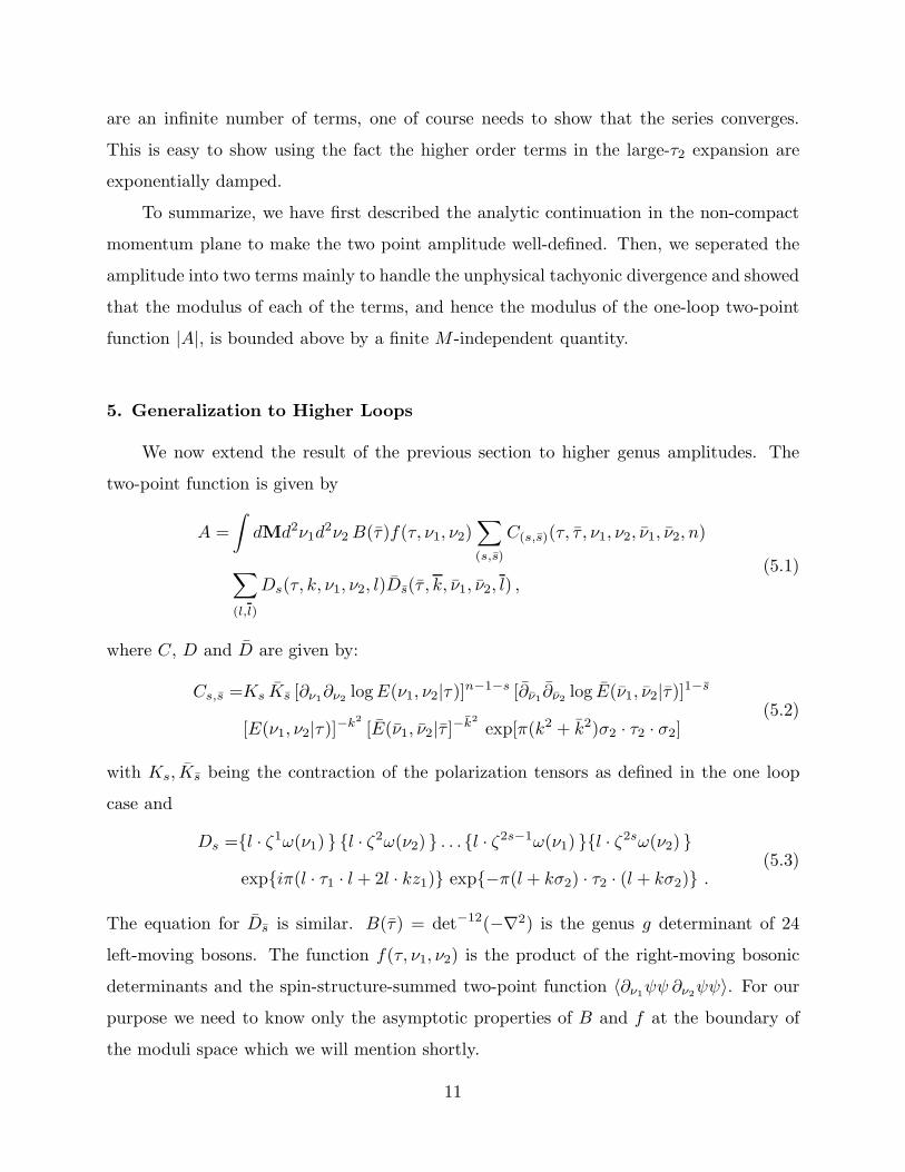
are an infinite number of terms, one of course needs to show that the series converges.

This is easy to show using the fact the higher order terms in the large-τ2 expansion are

exponentially damped.

To summarize, we have first described the analytic continuation in the non-compact

momentum plane to make the two point amplitude well-defined. Then, we seperated the

amplitude into two terms mainly to handle the unphysical tachyonic divergence and showed

that the modulus of each of the terms, and hence the modulus of the one-loop two-point

function |A|, is bounded above by a finite M -independent quantity.

5. Generalization to Higher Loops

We now extend the result of the previous section to higher genus amplitudes. The

two-point function is given by

A =

∫

dMd2ν1d2ν2B(τ)f(τ, ν1, ν2)

∑

(s,s)

C(s,s)(τ, τ , ν1, ν2, ν1, ν2, n)

∑

(l,l)

Ds(τ, k, ν1, ν2, l)Ds(τ , k, ν1, ν2, l) ,(5.1)

where C, D and D are given by:

Cs,s =Ks Ks [∂ν1∂ν2

logE(ν1, ν2|τ)]n−1−s [∂ν1

∂ν2log E(ν1, ν2|τ)]

1−s

[E(ν1, ν2|τ)]−k2

[E(ν1, ν2|τ ]−k2

exp[π(k2 + k2)σ2 · τ2 · σ2](5.2)

with Ks, Ks being the contraction of the polarization tensors as defined in the one loop

case and

Ds ={l · ζ1ω(ν1) } {l · ζ2ω(ν2) } . . .{l · ζ

2s−1ω(ν1) }{l · ζ2sω(ν2) }

exp{iπ(l · τ1 · l + 2l · kz1)} exp{−π(l + kσ2) · τ2 · (l + kσ2)} .(5.3)

The equation for Ds is similar. B(τ) = det−12(−∇2) is the genus g determinant of 24

left-moving bosons. The function f(τ, ν1, ν2) is the product of the right-moving bosonic

determinants and the spin-structure-summed two-point function 〈∂ν1ψψ ∂ν2

ψψ〉. For our

purpose we need to know only the asymptotic properties of B and f at the boundary of

the moduli space which we will mention shortly.

11

5.1. Analytic Continuation

As in the one-loop case, the integral expression (5.1) is naively divergent at the bound-

ary of the moduli space and we need to define the amplitude through analytic continuation.

For consistency, the analytic continuation employed in eq. (4.8) should work here too. To

see that it does, we need to consider in somewhat detail the boundary of the moduli space

of the higher genus Riemann surfaces. This is a rather well-studied subject [15,16,17]. For

our purposes, we can regard the boundary of the moduli space as consisting of two distinct

kind of degenerations of the Riemann surface:

1. Pinching along a homologically trivial cycle:

Under this, a genus g1 + g2 Riemann surface splits into two disjoint Riemann surfaces

(having one puncture each) of genuses g1 and g2. It is not difficult to see that such a

pinching factorizes the present two-point function in such a way that one of the factors

always equals one-point function of a tachyon at some loop. Since the latter quantity is

zero, the contribution of this kind of degeneration is zero. We shall therefore consider

degeneration along only the homologically nontrivial cycles henceforth.

2. Pinching along a homologically nontrivial cycle:

Under this kind of a degeneration a genus g + 1 surface reduces to a genus g surface

with two punctures. We need to know how the various factors in (5.1) behave under this

kind of a degeneration. The behaviour of C,D, D can be read off from the behaviour of

the period matrix τ and the abelian differentials ωI . The latter are given as follows. Let

τ IJ , I, J = 1, 2, . . . , g be the period matrix and ωI , I = 1, 2, . . . , g the abelian differentials

of the genus g Riemann surface obtained after the degeneration. Also, let a and b be the two

punctures. Then near the boundary of the moduli space corresponding to this degeneration,

the period matrix and abelian differentials of the original genus g + 1 Riemann surface is

given by

τ →

[

τIJ

∫ b

aωI

∫ b

aωJ τ00

]

,

ω0(ν1) →∂ν1log

[

E(a, ν1)

E(b, ν1)

]

.

(5.4)

where

τ00 →−i

π(log t

2− logE(a, b)) +O(t) as t→ 0.

12

Keeping in mind that there is an unphysical tachyon in the L0 = 1 spectrum of the left-

moving bosonic string (prior to the Re τ integration), we can infer the following asymptotic

form of B(τ):

B(τ) = (q0)−2B1(q0, qI) +B2(q0, qI) (5.5)

where B2 is finite over the entire moduli space and B1 is finite at the specific degeneration

of the Riemann surface under consideration. Since there is no such divergence from the

right sector, the asymptotic form of f is:

f(τ, ν1, ν2) = [1 +O(q20)]f1(qI , ν1, ν2) (5.6)

which is finite over the entire moduli space. Here qI = exp[iπτII ] and similarly for the

barred terms.

Combining all this, the asymptotic behaviour of A at this degeneration is given by

A∞ =

∫

dMd2τ00

∫

d2ν1d2ν2(q0)

−2[exp{−iπz01(k2 − k2)}]

[exp{−πσ02 Imτ00 (k2 + k2)}] exp[πσ0

2 Imτ00 σ02(k2 + k2)]Dn−1D1

(5.7)

where dM is a measure factor whose explicit form is not important for our purpose except

that it is independent of Re τ00. We have explicitly verified this fact in the two-loop

case [15]. For higher loops the measure factors in terms of the period matrix are quite

complicated for explicit verification. However, from the form of the measure in the Fenchel

Nielsen parametrization [10] we believe that it is true also at higher loops.

Going through steps similar to the ones in the one-loop case (i.e imposing modular

invariance Re τ00 → Re τ00 + 1 and then doing the Re τ00 integration), we arrive at

A∞ =

∫

dMdImτ00

∫

d2ν1d2ν2 exp{2π Imτ00 σ

02(1 − σ0

2)(−k2)}

∑

l,l

δ(l20−l2

0),−2

δ(l0·k−l0·k),n{l · ζ1ω(ν1) } {l · ζ

2ω(ν2) } . . .{l · ζ2s−1ω(ν1) }{l · ζ

2sω(ν2) }

{l · ζ1ω(ν1) } {l · ζ2ω(ν2) } . . . {l · ζ

s−1ω(ν1) } {l · ζsω(ν2) }

exp{−2πImτ00(l0 + kσ0

2)2} LgLg

(5.8)

where

Lg = exp{iπ(lI ReτIJ lJ + 2lI · kzI

1)} exp{−π(l + kσ2)I · ImτIJ · (l + kσ2)

J} . (5.9)

13

and its conjugate is Lg.

We see, therefore, that the amplitude is well-defined under the same analytic contin-

uation (4.8) as used in the one-loop case.

5.2. Bound on the two-point function

We now prove M -independence of the two-point function in higher loops.

Consider the moduli space after pinching any one non-zero homology cycle labeled by

‘0’, As in the one-loop case, we substitute (5.5) for B(τ) in (5.1), and divide A into two

parts:

A = A1 + A2, (5.10)

Here A1 and A2 correspond to the two terms (q0)−2B1(q0, qI) and B2(q0, qI) in (5.5)

respectively.

Since B2(q0, qI) is finite, the integrand of A2 is finite over the entire moduli space. We

can show that the modulus of A2 is bounded above by a finite M independent quantity

following the steps presented for one-loop.

A1 contains the unphysical tachyonic divergences. When only cycle ‘0’ is pinched and

no other then we can deal with the tachyonic divergence as in the one-loop case. At higher

loops, however, we have to take into account simultaneous pinching of more than one non-

trivial homology cycles. For example, if an additional cycle labeled by ‘1’ is pinched along

with ‘0’ then we have additional divergences. In this case B1(τ) can be written as

(q0)−2B1(τ) = (q0)

−2B(1)1 (q0, qI) + (q1)

−2B(2)1 (q0, qI) + (q0)

−2(q1)−2B

(3)1 (q0, qI), (5.11)

where the B coefficients on the right have no singularities at either of the two degenerations.

Correspondingly A1 now has three possible divergent terms

A1 = A(1)1 +A

(2)1 + A

(3)1 . (5.12)

It is now evident that A(1)1 and A

(2)1 are similar to the one loop A1 which can be

handled by integrating the real part of the appropriate period matrix element. So, these

two terms are again bounded by some finite M independent quantity.

14

The non-trivial term different from the one loop is A(3)1 . We have to integrate over the

real part of both the period matrix elements which dominate in the simultaneous pinching

of the two homologically non-zero cycles. This will lead to a restricted lattice sum which

can again be handled in exactly the same fashion as for the one loop.

It is straightforward to extend the procedure of seperating A1 (5.12) into various

terms under simultaneous pinching of arbitrary number of non-zero homology cycles at

every order in string loop and showing that each of the terms is finite and bounded above

by an M independent finite quantity.

6. Conclusions

The real part of A equals δM2 and the imaginary part equals, by the optical theorem,

ΓM , where Γ is the decay rate. Since |A| is bounded by an M independent constant, it

follows that both the mass correction δM as well as the width Γ are vanishingly small if

the tree-level mass is sufficiently large:

δM ≤ O(1/M) ; Γ ≤ O(1/M). (6.1)

One immediate consequence of our result is that it partially answers our original ques-

tion of why the degeneracy of even the nonsuper states agrees with the Sen entropy of the

associated black holes. We have proved here a perturbative nonrenormalization valid to

all loops. The agreement with the entropy suggests that it should be valid even nonper-

turbatively. There are a number of related issues that are currently under investigation.

Besides the entropy, the gyromagnetic ratios of the nonsuper states are also known to be

in agreement with those of the associated black holes [6,5]. We therefore expect a similar

nonrenormalization of the gyromagnetic ratio as well. The perturbative heterotic state

considered here, which has winding and momentum along the internal torus is dual to a

D-string in Type-I theory. It is interesting to know if a similar nonrenormalization holds

for the D-string. In particular, the large mass limit considered here appears to be related

to the large-N limit in the gauge theory on the D-string. More generally, one expects a

similar nonrenormalization for a host of magnetically charged as well as dyonic states that

are S-dual to the purely electrically charged states discussed here.

15

In this paper we have discussed black holes with zero area. For black holes with

nonzero area, both in the supersymmetric as well as nearly supersymmetric cases, there

is already an impressive agreement between the degeneracy of the string states and the

Bekenstein-Hawking entropy [18,19,20]. Furthermore, the emission and absorption proper-

ties of these black holes also match those of the corresponding string states [21,22,23,24,25].

Indeed, the entropy-matching seems to work even for a few nonsuper states [7,26,27]. It

would be interesting to see if these states satisfy mass-nonrenormalization of the kind

presented here. Previous discussions of nonrenormalization in the context of nearly super-

symmetric black holes with nonzero area can be found in [28,29].

We end with a few comments and speculations. Our results are in accord with the

general correspondence, pointed out in [30], between perturbative string states and black

holes. By this correspondence the two degeneracies match at a specific value of the coupling

where the quantum correction to the spectrum is becoming appreciable. However, if there

is no renormalization of the spectrum, as in our case, the degeneracies can be compared at

all values of the coupling. The nonrenormalization that we have found is quite surprising

because it is not a consequence of any apparent symmetry. It may be that there is a hidden

gauge symmetry of string theory that is responsible for this nonrenormalization.

Our results indicate that there is an infinite tower of very massive nonsuper states

with N = 1 and arbitrary N , which is very similar to the infinite tower of super states

with N = 12 and arbitrary N . The spectrum of super states has important application to

the dynamics of the theory. For instance, in N = 2 string theories one can construct a

generalized Kac-Moody Lie superalgebra in terms of super states which governs the form

of the perturbative superpotential [31]. It would be interesting to see if the nonsuper states

discussed here or their duals can be used to obtain additional insight into the dynamics.

Acknowledgements

We would like to thank Indranil Biswas, Pablo Gastesi, Ashoke Sen, and Lenny

Susskind for useful discussions, and the organizers of the 1996 Puri Workshop for invit-

ing us to a very stimulating meeting where this work was initiated. G.M. would like to

acknowledge the hospitality of CERN theory division where part of the work was done.

16

References

[1] E. Witten and D. Olive, Phys. Lett. B78 (1978) 97.

[2] A. Dabholkar and J. A. Harvey, Phys. Rev. Lett. 63 (1989) 478; A. Dabholkar, G.

Gibbons, J. A. Harvey, and F. R. Ruiz-Ruiz, Nucl. Phys. B340 (1990) 33.

[3] A. Sen, Mod. Phys. Lett. A10 (1995) 2081, hep-th/9504147.

[4] A. W. Peet, Nucl. Phys. B446 (1995) 211, hep-th/9504097.

[5] M. Duff, J. T. Liu, and J. Rahmfeld, Nucl. Phys. B494 (1997) 161, hep-th/9612015.

[6] M. Duff and J. Rahmfeld, Nucl. Phys. B481 (1996) 332, hep-th/9605085.

[7] A. Dabholkar, Phys. Lett. B402 (1997) 53; hep-th/9702050.

[8] A. Dabholkar, J. P. Gauntlett, J. A. Harvey, and D. Waldram,

Nucl. Phys. B474 (1996) 85, hep-th/9511053.

[9] E. Verlinde and H. Verlinde, Phys. Lett. B192 (1987) 95.

[10] E. D’Hoker and D. H. Phong, Rev. Mod. Phys. 60 (1988) 917.

[11] D. Mumford, Tata Lectures on Theta, Birkhauser (1983).

[12] R. Dijkgraaf, E. Verlinde and H. Verlinde, Comm. Math. Phys. 115 (1988) 649.

[13] E. D’Hoker and D. H. Phong, Phys. Rev. Lett. 70 (1993) 3292.

[14] J.L. Montag and W.I. Weisberger, Nucl. Phys. B363 (1991) 527 .

[15] G. Moore, Phys. Lett. B176 (1986) 369.

[16] R. Dijkgraaf, E. Verlinde and H. Verlinde, Comm. Math. Phys. 115 (1988) 649.

[17] J.D. Fay, Theta functions on Riemann surfaces, Lecture Notes in Mathematics,

Vol.352 (Springer, Berlin, 1973) .

[18] A. Strominger and C. Vafa, Phys. Lett. B379 (1996) 99, hep-th/9601029.

[19] G. Horowitz and A. Strominger, Phys. Rev. Lett. 77 (1996) 2368, hep-th/9602051.

[20] C. G. Callan and J. M. Maldacena, Nucl. Phys. B475 (1996) 645, hep-th/9602043.

[21] A. Dhar, G. Mandal and S.R. Wadia, Phys. Lett. B388 (1996) 51, hep-th/9605234.

[22] S. Das and S. Mathur, Nucl. Phys. B478 (1996) 561, hep-th/9606185; Nucl. Phys.

B482 (1996) 153, hep-th/9607149.

[23] J. Maldacena and A. Strominger, Phys. Rev. D55 (1997) 861, hep-th/9609026.

[24] S.S. Gubser and I. Klebanov, Nucl. Phys. B482 (1996) 173, hep-th/9608108.

[25] C. Callan, S.S. Gubser, I. Klebanov and A. Tseytlin, Nucl. Phys. B489 (1997) 65,

hep-th/9610172.

[26] G. Horowitz, D. Lowe, and J. Maldacena, Phys. Rev. Lett. 77 (1996) 430, hep-

th/9603195.

[27] D. M. Kaplan, D. A. Lowe, J. M. Maldacena, and A. Strominger, Phys. Rev. D55

(1997) 4898, hep-th/9609204.

[28] J. Maldacena, Phys. Rev. D55 (1997) 7645, hep-th/9611125; S.F. Hassan and S.R.

Wadia, Phys. Lett. B402 (1997) 43, hep-th/9703163.

[29] S. Das, hep-th/9703146.

[30] G. Horowitz and J. Polchinski, hep-th/9612146.

[31] J. Harvey and G. Moore, hep-th/9609017.

17