Seediscussions,stats,andauthorprofilesforthispublicationat:https://www.researchgate.net/publication/235470713

Functionalrenormalizationforquantumphasetransitionswithnonrelativisticbosons

ArticleinPhysicalReviewB·February2008

DOI:10.1103/PhysRevB.77.064504·Source:arXiv

CITATIONS

37

READS

16

1author:

ChristofWetterich

UniversitätHeidelberg

316PUBLICATIONS14,598CITATIONS

SEEPROFILE

AllcontentfollowingthispagewasuploadedbyChristofWetterichon01December2016.

Theuserhasrequestedenhancementofthedownloadedfile.Allin-textreferencesunderlinedinbluearelinkedtopublicationsonResearchGate,lettingyouaccessandreadthemimmediately.

arX

iv:0

705.

1661

v3 [

cond

-mat

.sup

r-co

n] 2

9 Fe

b 20

08

Functional renormalization for quantum phase transitions with non-relativistic bosons

C. WetterichInstitut fur Theoretische Physik

Universitat Heidelberg

Philosophenweg 16, D-69120 Heidelberg

Functional renormalization yields a simple unified description of bosons at zero temperature, inarbitrary space dimension d and for M complex fields. We concentrate on nonrelativistic bosons andan action with a linear time derivative. The ordered phase can be associated with a nonzero densityof (quasi) particles n. The behavior of observables and correlation functions in the ordered phasedepends crucially on the momentum kph, which is characteristic for a given experiment. For the

dilute regime kph & n1/d the quantum phase transition is simple, with the same “mean field” critical

exponents for all d and M . On the other hand, the dense regime kph ≪ n1/d reveals a rather rich

spectrum of features, depending on d and M . In this regime one observes for d ≤ 3 a crossover to arelativistic action with second time derivatives. This admits order for d > 1, whereas d = 1 showsa behavior similar to the low temperature phase of the classical two-dimensional O(2M)-models.

I. INTRODUCTION

The ground state of many quantum systems can undergoa second order phase transition if the density, concentra-tion, external fields or some effective coupling constants arevaried. An example is the transition from para- to ferro-magnetism for bosonic atoms with spin. Bosonic quasi-particles also describe the quantum phase transition forstrongly correlated electrons in case of anisotropic antifer-romagnetic order. We address here only systems where thelow energy excitations are bosons - they can be relevantalso for correlated electrons, if the fermionic excitationsare gapped.

An effective description accounts for a transition from an“ordered phase” with a nonzero continuously varying den-sity of bosonic excitations to a “disordered phase” wherethis density vanishes. At zero temperature the boson den-sity can often be characterized by a condensate, which isdescribed by the nonvanishing expectation value of a (com-plex) field. In a broad sense such a condensate can beassociated with order, while for the disordered phase theexpectation value vanishes. Such transitions between a dis-ordered or “symmetric” phase and an ordered phase withspontaneous symmetry breaking are therefore described byBose-Einstein condensation in a gas of interacting bosons.In this picture the parameter driving the phase transi-tion can be associated with an effective chemical poten-tial σ. Universality of the critical behavior near secondorder phase transitions implies that many key features ofquantum phase transitions are independent of the particu-lar “microscopic” physical systems. With ultracold bosonicatoms new ways of experimental investigation of such sys-tems open up.

For dilute systems, many features of quantum phasetransitions for bosons are well understood, and many de-tails of the critical behavior in various dimensions areknown. The basic aspects are visible in a mean field theoryand perturbation theory [1]. The use of several methods,including mapping to fermionic systems and bosonizationin one dimension, together with strong universality argu-ments based on the renormalization group, allows for the

computation of critical exponents and correlation functions[2]. One finds a rather simple picture with mean field crit-ical exponents. This picture is valid, however, only as longas the system is sufficiently dilute. In this paper we ex-tend the discussion to dense systems. For one- and two-dimensional systems we will find qualitative changes. Theyare induced by the fluctuations of the Goldstone boson,which is characteristic for the spontaneous breaking of acontinuous symmetry. In three dimensions, these effectsare logarithmic - still sufficient for a cure of the infraredproblems in many previous treatments [3]. This cure issimilar to other renormalization group approaches [4, 5].

In order to define the notion of dense and dilute, oneshould compare a typical physical length scale, l, withthe average distance between particles, D ∼ n−1/d. Fordense systems one has l ≫ D, whereas dilute systems obeyl ≪ D. As a first attempt one could try to use the cor-relation length ξ as physical length scale. This works wellin the disordered phase where ξ is finite away from thephase transition. In the ordered phase, however, the spon-taneous symmetry breaking of an abelian continuous sym-metry leads to superfluidity. For a nonzero condensate thesystem has always a gapless (“massless”) mode - the Gold-stone boson. The correlation length is infinite such thatthe system would appear “dense” for any nonvanishing n.

In practice, a given experiment will always involve aneffective momentum scale kph, for example the inverse ofthe wave length used to probe the system. Technically,the “physical momentum scale” kph may correspond to themomentum in some relevant Green’s functions and act asan (additional) infrared cutoff for the fluctuations. Thesmallest possible value of kph is given by the inverse size ofthe experimental probe. Instead of ξ−1 we may thereforecompare the physical momentum scale kph with the scale

kF ∼ n1/d. For kF ≪ kph the particle density only inducessmall corrections and the Bose gas is dilute. In contrast,the dense regime for kph ≪ kF corresponds to a situation

where a characteristic inter-particle distance D ∼ k−1F is

small as compared to a typical experimental length scalel ∼ k−1

ph . We use the concepts “dilute” and “dense” here ina rather general sense since we do not specify l a priori.

2

In the ordered phase the quantum fluctuations with lowmomenta, ~q2 = k2 , k ≪ kF , are dominated by the Gold-stone boson. We will call this the “Goldstone regime”. Inthree dimensions the Goldstone fluctuations play a quan-titative role, but do not change the qualitative behavior,except for the extreme infrared. (Due to a logarithmicrunning of dimensionless couplings the qualitative changesmay only occur for exponentially small momentum scales.)Typically, fluctuations on length scales larger than the scat-tering length a give only small corrections. For kph ≪ a−1

the precise value of kph becomes unimportant - the mostimportant effective infrared cutoff is set by a−1. In thiscase we may consider a system with akF ≪ 1 as dilute,independent of kph. In contrast, for d = 1, 2 the Goldstonefluctuations always play an important role for kph ≪ kF .In this case the value of kph matters and needs to be con-sidered as a separate physical scale.

The simple critical behavior of the dilute regime alwaysapplies for the disordered phase since n = 0. In contrast,the understanding of the ordered phase is more subtle, inparticular for lower dimensional systems, d = 1 or d = 2.The dilute regime kph ≫ kF remains simple, with similarproperties as for the disordered phase. As kph becomessmaller than kF we have to deal with a dense Bose gaswhere n sets a new scale. Following the scale dependence of“running” renormalized couplings one observes a crossoverto the “Goldstone regime”, with new qualitative properties.We argue that for d = 1 and d = 2 the Goldstone regime iseffectively described by a relativistic action with two timederivatives. It therefore shares common features with theclassical O(2M)-models in dimension d + 1. In particular,for d = 1 and M = 1 this implies the characteristic behav-ior of the low temperature phase in the Kosterliz-Thouless[6] phase transition.

We propose here a simple unified picture for the prop-erties of the quantum phase transition which is valid onall scales. It is based on the functional renormalizationgroup [7] for the average action [8], [9], [10]. Within a sim-ple φ4-model it describes the quantum phase transition foran arbitrary number of space dimensions d and an arbi-trary number of components M . Within the same modelwe can explore the flow in the disordered and the orderedphase. For low dimensions d = 1 or d = 2 we find severalinteresting crossover phenomena, indeed associated to thenontrivial physics of Goldstone bosons in low dimensions.This crossover persists for d = 3, but wide scale separationsoccur due to logarithmic running. The case d = 3 can beconsidered as the boundary dimension for the relevance ofthe Goldstone regime.

All of the relevant physics is non-perturbative (with afew exceptions) and involves long range excitations. Wedo not limit our investigation to small interaction strength.We therefore rely heavily on the capability of modern ap-proaches to functional renormalization where the variationof an effective infrared cutoff enables the exploration of sys-tems with massless excitations (infinite correlation length)in a nonperturbative context for arbitrary d [8, 9, 10, 11].For the regime kph ≫ kF the merits of our approach lie, forthe time being, more in the simplicity of the unified pic-

ture rather than in new quantitative results. In contrast,the flow for the dense systems, kph ≪ kF , reveals featuresthat have attracted less attention so far.

Our approach is based on a functional integral formu-lation where the bosonic excitations are associated to acomplex field χ. It is formulated in a d + 1 dimensionaleuclidean space with d space dimensions and an euclideantime τ . (For nonzero temperature T euclidean time param-eterizes a torus with circumference T−1.) The transitionfrom the Hamiltonian formulation with operators to thefunctional integral (or Lagrange formulation) with fieldsis sometimes subtle [12], [13], [2]. Two classes of systemscan be distinguished, according to the presence of a linearτ -derivative or not. In a rather general approach we mayconsider a microscopic or “classical” action

S =

∫

x

χ∗(

S∂τ − V ∂2τ − ∆

2MB− σ

)χ + Sint (1)

where∫x

=∫

dτ∫

dd~x. We will assume that Sint describes a

local interaction, involving powers of χ∗χ without deriva-tives. For arbitrary S and V the action (1) is invariantunder euclidean time reversal τ ↔ −τ , χ ↔ χ∗.

The case S = 0 is special, however. The system possessesnow an enhanced rotation symmetry SO(d + 1), mixingspace coordinates ~x and the time coordinate τ . Indeed,a simple multiplicative rescaling of time or space coordi-nates brings the derivatives to the form (∂2

τ + ∆). Therelativistic excitation spectrum can be directly seen by an-alytic continuation to “real time”, τ = it. After suitablerescalings we may set V = 1, 2MB = 1, such that eq. (1)reduces to the classical O(2M)-model in dimension d + 1,if χ has M complex components. (For M > 1 suitablesums over components are implied in eq. (1)). Functionalrenormalization has already provided a unified picture forthe phase transition in classical O(N)-models for arbitraryd [9, 10, 11], including the Kosterlitz-Thouless phase tran-sition for d + 1 = 2 and M = 1 [14]. Due to the en-hanced symmetry the vanishing of the coefficient linear in∂τ (S = 0) is stable under the renormalization flow.

In this paper we search for a similar unified picture forthe “nonrelativistic bosons” with S 6= 0. We will con-centrate on the simplest case V = 0 where by a suit-able rescaling we may choose S = 1. In Minkowskispace the microscopic action is now invariant under Galilei-transformations. We emphasize, however, that V = 0 isnot protected by a symmetry and second τ -derivatives willbe generated by the functional renormalization flow. ForT = 0 this comes together with the higher order gradientterms requested by Galilei invariance.

Even though we concentrate in this paper on the Galilei-invariant setting with V = 0, the discussion in sect. VIIIwill also cover the more general case of a microscopic ac-tion (1) with S 6= 0 , V 6= 0. We first specialize to onecomponent and extend the discussion to M -components insect. X. An overview over the different regimes for arbi-

trary d, M and S/√

V , together with our main results, canbe found in the conclusions.

3

Our paper is organized as follows. In order to specify ourmodel and to fix notations we recall the functional integralformulation and functional renormalization in sect. II. Insect. III we derive the flow equations for the renormalizedcouplings for arbitrary d (M = 1). Sect. IV gives a briefdescription of running couplings in the disordered phase.We discuss the fixed points and the associated scaling be-havior relevant for the quantum phase transition in sect.V. Sects. IV and V reproduce the known results for non-relativistic quantum phase transitions [2] within the frame-work of functional renormalization. They may be skippedby the reader familiar with the subject. In sect. VI we de-rive the flow equations for the ordered phase, first within atruncation where second τ -derivatives are neglected. Sect.VII distinguishes the “linear regime” relevant for dilutesystems from the Goldstone regime which is important fordense systems. For d < 2 our simplest truncation yields anattractive fixed point with nonzero order parameter anddensity. For d = 1 this fixed point will persist for extendedtruncations, while it turns out to be an artefact of thetruncation for d > 1.

For d ≤ 3 the large time behavior within the orderedphase is governed by a term quadratic in the τ -derivatives∼ V . We show in sect. VIII how this term is generated bythe flow, even if it vanishes for the microscopic action. Fordense systems and d < 3, the “relativistic dynamic term”∼ V will always dominate over the term linear in ∂τ . Therunning coupling S(k) vanishes with a power of k. In con-trast, for the boundary dimension d = 3 the vanishing ofS(k) is only logarithmic. The corresponding change in thepropagator induces qualitative changes for the renormaliza-tion flow and phase structure for one- and two-dimensionalsystems. They constitute the main result of the presentpaper. We find that the long distance behavior of corre-lation functions is similar as for the classical O(2)-modelsin d + 1 dimensions. In particular, for d = 1 the orderedphase of the non-relativistic model behaves similar to thelow temperature phase of the two-dimensional Kosterlitz-Thouless phase transition. We associate the Tomonaga-Luttinger liquid [15] to this phase. In sect. IX we discussthe Goldstone regime in terms of non-linear σ-models. Ourapproach permits a unified view of the linear ϕ4-modelsand non-linear σ-models. Sect. X is devoted to an exten-sion of our discussion to M complex bosonic fields. Wepresent conclusions and outlook in sect. XI.

II. FUNCTIONAL INTEGRAL AND

FUNCTIONAL RENORMALIZATION

We start with the partition for a nonrelativistic bosonicparticle for M = 1

Z =

∫Dχ exp(−S[χ]), (2)

with action S[χ] given by eq. (1), with S = 1, V = 0. Thecomplex field χ may be expressed by its Fourier modes

χ(x) = χ(τ, ~x) =

∫

~q

ei~q~xχ(τ, ~q) =

∫

q

eiqxχ(q), (3)

with

q = (q0, ~q) ,

∫

q

=

∫

~q

∫

q0

,

∫

q0

=1

2π

∞∫

−∞

dq0,

∫

~q

= (2π)−d

∫dd~q . (4)

For nonzero temperature T the Euclidean time τ parame-terizes a circle with circumference Ωτ = T−1 and the Mat-subara frequencies q0 = 2πnT , n ∈ Z, are discrete, with∫

q0= T

∑n

.

In this paper we are interested in quantum phase transi-tions for T = 0. This phase transition occurs as the param-eter σ is varied from positive to negative values. We regu-larize the theory by a momentum cutoff ~q 2 < Λ2 and takeΛ → ∞ when appropriate. Furthermore, we assume theinvariance of the classical action (2) under a global abeliansymmetry of phase rotations χ → eiϕχ, corresponding toa conserved total particle number

N =

∫

~x

n(~x) = Ωd

∫

~q

n(~q), (5)

with Ωd the volume of d-dimensional space (Ωd+1 = ΩdΩτ ).Following the Noether construction we can express n(~q) bythe two point correlation function

n(~q) =1

Ωd+1

∫

q0

〈χ∗(q0, ~q)χ(q0, ~q)〉 −1

2. (6)

We may associate σ = σ − ∆σ with a chemical potential.Here our normalization of the additive shift ∆σ [13] and ofn(~q) is such that N = 0 for σ < 0 and N 6= 0 for σ > 0.If we interprete n = N/Ωd as the number density of somebosonic quasi particle, the quantum phase transition is atransition from a state with no particles to a state withnonzero particle density.

By a suitable rescaling of units of x, τ and χ we can

replace 2MB → 1 , σ → σ = 2MBσ/k2. Here we may

use some arbitrary momentum unit k in order to make allquantities dimensionless, or we may retain dimensionful

parameters by employing k = 1. (The parameters in Sint

have to be rescaled accordingly, see Ref. [16].) In the fol-lowing we will work with a basis of real fields χ1, χ2 definedby χ(x) = 1√

2

(χ1(x) + iχ2(x)

)such that χa(−q) = χ∗

a(q).

The connected part of the two point function describes thepropagator G

〈χ∗a(q)χb(q

′)〉 = Gab(q, q′) + 〈χ∗

a(q)〉〈χb(q′)〉. (7)

For a translation invariant setting, G is diagonal in momen-tum space

Gab(q, q′) = Gab(q)δ(q − q′), (8)

4

with δ(q − q′) = (2π)d+1δ(q0 − q′0)δd(~q − ~q ′). Also, trans-

lation invariance implies for a possible order parameter〈χa(q)〉 =

√2φ0δ(q)δa1 with real φ0. Here we have cho-

sen the expectation value in the one-direction without lossof generality.

We assume a repulsive two particle interaction (λ > 0)

Sint =λ

2

∫

x

(χ∗(x)χ(x)

)2=

λ

8

∫

x

(χa(x)χa(x)

)2. (9)

After the rescaling the mass dimensions are x ∼ µ−1 , τ ∼µ−2 , ~q ∼ µ , q0 ∼ µ2 , χ ∼ µ

d2 , σ ∼ µ2 , n ∼ µd, such

that λ ∼ µ2−d. Already at this point one sees the crucialrole of the dimension d. For d = 3 the coupling λ has thedimension of a length. After a suitable renormalization itcorresponds to the scattering length a ∼ λ. In the vac-uum (T = 0 , n = 0 , σ = 0) the renormalized interactionstrength λ sets the only scale, besides the ultraviolet cut-off Λ. As a consequence, those correlation functions thatare independent of Λ can only depend on dimensionlesscombinations, as λ~q and λ2q0. For example, the two pointfunction takes the form G = A(~q2+iSq0+V q2

0)−1 with real

functions A, S, and V/λ2 depending on these dimensionlesscombinations. A nonzero density introduces an additionalscale kF . The long distance physics will now depend onthe dimensionless concentration c = akF ∼ λn1/3.

In one dimension (d = 1) the interaction strength scalesλ ∼ µ. Now a length scale is set by λ−1. For nonzero den-sity the macroscopic physics can depend on dimensionlesscombinations, as n/λ. Indeed, for λ → ∞ the repulsion be-comes infinite such that a particle can never pass anotherparticle. (This permits the mapping to a non-interactingFermi gas [2].) The combination n/λ is a measure of howmany interparticle distances a particle can travel before be-ing repulsed. It therefore defines an effective volume whereit can move.

The case d = 2 is special because λ is dimensionless.In the vacuum no length scale except the cutoff is present.The running coupling vanishes logarithmically for large dis-tances (see sect. IV), such that the long distance physicsis described by a free theory. In the two point correlationG = A(~q2 + iSq0 + V q2

0)−1 the functions S, A can only de-

pend on q0/~q2 and λ, besides cutoff effects involving ~q2/Λ2.No coupling V is allowed. A nonzero density sets again afurther scale kF ∼ n1/2. For momentum scales below kF

the running of λ gets modified and the macrophysics isno longer a free theory. In particular, the dimensionlesscombination V n will now play an important role.

We will conveniently work with the effective action Γ[φ]which generates the 1PI correlation functions. It ob-tains by introducing local linear sources j(x) for χ(x) andperforming a Legendre transform of ln Z[j], with φ(x) =〈χ(x)〉|j in the presence of sources

Γ[φ] = − lnZ[j] (10)

+

∫

q

(φ∗(q)j(q) + j∗(q)φ(q)

).

The difference between S and Γ results from quantumfluctuations. We include these fluctuation effects stepwise

by introducing first an infrared cutoff which suppresses thefluctuations with momenta ~q 2 < k2. This is done byadding to the action (2) an infrared cutoff term [8]

∆kS =

∫

q

Rk(~q)χ∗(q)χ(q). (11)

In turn, the effective action is now replaced by the averageaction Γk which depends on k [9], [10]. With Rk(~q) diverg-ing for k → ∞ all fluctuations are suppressed in this limitand one finds Γk→∞ = S. On the other hand Rk(~q) = 0for k → 0 implies Γk→0 = Γ. The average action there-fore interpolates smoothly between the classical action fork → ∞ and the effective action for k → 0. Its dependenceon k obeys an exact flow equation [9]

∂kΓk[φ] =1

2Tr∂kR(Γ

(2)k [φ] + R)−1 (12)

with R(q, q′) = Rk(~q)δ(q − q′). The second functional

derivative Γ(2)k is given by the full inverse propagator in

the presence of “background fields” φ. For a homogeneous

background field one has Γ(2)k (q, q′) = P (q)δ(q − q′) with

P a matrix in the space of fields (φ1, φ2). The trace in-volves a momentum integration and a trace over internalindices. Taking functional derivatives of eq. (12) yields theflow of all 1PI-vertices or associated Green’s functions. Eq.(12) therefore describes infinitely many running couplings.For homogeneous background fields φ eq. (12) takes theexplicit form (with tr the internal trace)

∂kΓk =Ωd+1

2tr

∫

q

∂kRk(~q)(P (q) + Rk(~q)

)−1. (13)

The precise shape of the cutoff function Rk is, in principle,arbitrary.

For ∂kRk decaying sufficiently fast for large ~q2 the ~q-integration on the r.h.s. of the flow equation (12) or (13) isultraviolet finite. Instead of an explicite ultraviolet cutofffor the momentum integration, we can therefore define ourmodel by specifying the form of Γk at some cutoff scalek = Λ. The short distance physics is now given by the“initial value” ΓΛ. For example, the bare coupling λ inthe action can be replaced by a coupling λΛ, given by thefourth derivative of ΓΛ. This definition has the advantagethat momentum integrals can always be performed over aninfinite range. The relation between the action S (withmomentum cutoff) and the microscopic effective action ΓΛ

(without momentum cutoff) can be established by a oneloop calculation. (In particular, this absorbs the shift ∆σin the chemical potential which is generated by the transi-tion from a Hamiltonian formalism to the functional inte-gral [13].)

Our task will be to follow the flow of Γk from an ini-tial value given at k = Λ towards k = 0. From Γk=0 = Γthe 1PI-correlation functions of the quantum theory can beextracted by simple functional differentiation. Despite itsconceptually simple one loop form, the exact flow equation(12) remains a complicated functional differential equation.For approximate solutions we truncate the most general

5

form of Γk. In the present investigation we will use verysimple truncations, involving only a small number of cou-plings. The minimal set involves only three k-dependentrenormalized couplings S, m2 and λ, according to the trun-cation

Γk =

∫

x

φ∗(S∂τ − ∆ + m2)φ +

λ

2(φ∗φ)2

. (14)

Nevertheless, many characteristic properties of the quan-tum phase transition in arbitrary dimension d will be ac-counted for by this truncation. This also holds away fromthe phase transition for the disordered phase and for thedilute regime of the ordered phase. For the dense regimeof the ordered phase in d = 1, 2 we should add a term con-taining a second τ derivative as in eq. (1), such that theminimal set consists of four running coupling m2, λ, S andV . The coupling V is also needed for d = 3 if one attemptsquantitative accuracy or a correct description of the longdistance asymptotics.

In this paper we mainly concentrate on non-relativisticbosons with a linear τ -derivative in the action. The initialvalue ΓΛ is then given by eq. (14), with SΛ = 1 , m2

Λ = −σand λ = λΛ. (We will only briefly comment on the moregeneral case where a second τ -derivative ∼ VΛ is added tothe microscopic action.) The microscopic average actionΓΛ defines the model, which has only two parameters inour case, namely the rescaled chemical potential σ and themicroscopic interaction strength λΛ. This should be distin-guished from the truncation of Γk for k < Λ. In principle,all couplings allowed by the symmetries will be generatedby the flow. This holds even though ΓΛ has only two pa-rameters. Restricting Γk to a finite number of couplingsdefines the approximation scheme.

In the formal setting the physical n-point functions areonly recovered for k → 0. Nevertheless, the properties ofΓk for k > 0 also admit a physical interpretation. A typi-cal experimental situation has neither infinite volume norobservation devices working at infinite wavelength. Thisinduces a characteristic experimental or “physical” momen-tum scale kph, as mentioned in the introduction. Formally,this scale appears in the form of nonvanishing “external”momenta for the Green’s functions which are relevant fora given observation. Often kph acts as an effective infraredcutoff such that the evolution of these Green’s functions(with finite momenta) stops once k becomes smaller thankph. On the other hand, for k ≫ kph the external momentaare not relevant so that one may investigate the Green’sfunctions or appropriate derivatives at zero momentum.In a simplified approach we may therefore associate theGreens-functions derived from Γk=0 at finite physical mo-mentum |~q| ≈ kph with the Greens function extracted fromΓkph

at zero external momentum. In this picture we simplyshould stop the flow of Γk at the physical scale kph ratherthan considering the limit k → 0. The experimentally rele-vant Green’s functions can then be extracted from Γkph

. Ofcourse, such a procedure gives only a rough idea. In gen-eral, the Greens-functions will depend on several momenta.Even if only one momentum ~q is involved, the precise wayhow the flow is stopped by a physical infrared cutoff in-

volves “threshold effects” [10]. As a consequence, the pro-portionality coefficient between |~q| and kph will depend onthe particular definition of the n-point function.

The average action Γk has the same symmetries as themicroscopic action, provided one chooses a cutoff Rk con-sistent with the symmetries. We sketch in appendix G theconsequences of Galilei symmetry and local U(1) symme-try for the general form of Γk at T = 0 - more details canbe found in Ref. [17].

III. FLOW EQUATIONS FOR POINTLIKE

INTERACTIONS

We first truncate the average action in the pointlikeapproximation and keep only the lowest time and spacederivatives

Γk =

∫

x

Zφφ∗∂τ φ − Aφ∗∆φ + u(Aφ∗φ)

=

∫

x

Sφ∗∂τφ − φ∗∆φ + u(φ∗φ)

. (15)

Here we have introduced S(k) = Zφ(k)/A(k) and therenormalized field

φ = A1/2φ. (16)

We use notations where quantities with a bar denote thecouplings of the “unrenormalized field” φ, whereas therenormalized couplings of the field φ have no bar. At thescale k = Λ one has A(Λ) = AΛ = 1 so that φ and φ co-incide. In general, the couplings Zφ and A are evaluatedat a nonzero value of the renormalized field φ0. As a con-sequence, they need not to be equal in the ordered phase,even in presence of Galilei symmetry for T = 0 (cf. app.G).

We choose the infrared cutoff function [18]

Rk = A(k2 − ~q 2)θ(k2 − ~q 2). (17)

This cutoff violates Galilei symmetry, but our truncationwill neglect counterterms associated to anomalous Wardidentities - they vanish for k → 0. The initial values of ΓΛ

will be taken as

Zφ,Λ = AΛ = 1 , uΛ = m2Λφ∗φ +

1

2λΛ(φ∗φ)2,

m2Λ = −σ. (18)

Besides the rescaled chemical potential σ our model de-pends on the strength of the repulsive interaction, λΛ > 0.

By a rescaling of the momentum unit k → k/α the parame-ters and fields scale as m2

Λ → α2m2Λ , λΛ → α2−dλΛ , φ →

αd2 φ. Physical results for dimensionless quantities can

therefore only depend on scaling invariant combinations

as λΛ(m2Λ)

d−2

2 , ~q 2/m2Λ, q0/m2

Λ, ~q 2/Λ2. We notice againthe special role of d = 2 where λΛ is dimensionless.

The phase is determined by the properties of the effec-tive potential u for k → 0 (or k → 1/L with L the macro-scopic size of the experimental probe). In the ordered phase

6

the minimum of u occurs for φ0(k) 6= 0 and one observesspontaneous symmetry breaking (SSB) of the global U(1)-symmetry. In contrast, the disordered or symmetric phase(SYM) has φ0 = 0. For d = 1 we will encounter the bound-ary case where φ0(k) 6= 0 for arbitrarily small k, whileφ0(k = 0) = 0. (Typically φ0(k) vanishes with some powerof k.) Since many properties of this phase are analogousto the SSB phase for d > 1 we will use the name “orderedphase” also for this case, even though long range order doesnot exist in a strict sense for the infinite volume limit.

The flow of the average potential u follows by evaluat-ing eq. (12) for space- and time-independent φ, i.e. eq.(13). We use the fact that the potential depends only onthe invariant ρ = φ∗φ and uk(ρ) = Γk(φ)/Ωd+1. In ourtruncation the flow equation reads, using t = ln(k/Λ),

∂tu|φ =1

2

∫

q

tr∂tRkG. (19)

Here the propagator is a 2 × 2 matrix G = A−1G,

G−1 =

(q2 + u′ + 2ρu′′ , −Sq0

Sq0 , q2 + u′

), (20)

with q2 = ~q 2 for ~q 2 > k2 and q2 = k2 for ~q 2 < k2.Primes denote derivatives with respect to ρ. Introducingthe anomalous dimension

η = −∂t ln A (21)

we compute in app. A the flow equation for the averagepotential (at fixed φ instead of fixed φ) as

∂tu = ηρu′ +4vd

dSkd+2

(1 − η

d + 2

)

k2 + u′ + ρu′′√

k2 + u′√

k2 + u′ + 2ρu′′, (22)

where

v−1d = 2d+1π

d2 Γ

(d

2

). (23)

Eq. (22) is a nonlinear differential equation for a functionof two variables u(ρ, k), if η(k) and S(k) are known. Onemay solve equations of this type numerically [19].

We will choose here an even more drastic truncation anduse a polynomial expansion around the minimum of u. Inthe symmetric regime the minimum of u is at ρ = 0 andwe approximate

u = m2ρ +1

2λρ2. (24)

The corresponding flow equations for m2 = u′(0) , λ =u′′(0) read

∂tm2 = ηm2, (25)

∂tλ = 2ηλ +4vd

dS

(1 − η

d + 2

)kd+2

(k2 + m2)2λ2.

Inspection of eqs. (A.3), (A.4) shows that the system (25)is closed and does not involve higher derivatives of the po-tential as u(3) and u(4). For the SSB regime, with minimumof u(ρ) at ρ0 6= 0, one expands

u =λ

2(ρ − ρ0)

2. (26)

In this case the flow equations for ρ0 and λ also involve u(3)

and u(4). Neglecting these higher order couplings in oursimplest truncation one finds, from u′(ρ0) = 0 , u′′(ρ0) =λ, the flow of the minimum

∂tρ0 = − 1

λ∂tu

′(ρ0) (27)

= −ηρ0 +2vd

dS

(1 − η

d + 2

)λρ0

kd+1

√k2 + 2λρ0

(1

k2− 3

k2 + 2λρ0

).

The flow of the quartic coupling obeys now

∂tλ = 2ηλ − 2vd

dS

(1 − η

d + 2

)λ2 kd+1

√k2 + 2λρ0

(28)

1

k2− 3

k2 + 2λρ0− 3

2λρ0

(1

k4− 9

(k2 + 2λρ0)2

).

In the symmetric regime we find a (partial) fixed pointfor m2 = 0, while in the SSB one has a fixed point forρ0 = 0. These points coincide, with a quartic potentialu = 1

2λρ2. In turn, the flow for the quartic coupling

∂tλ = 2ηλ +4vd

dS

(1 − η

d + 2

)kd−2λ2 (29)

has a fixed point for λ = 0, corresponding to a free the-ory. In order to understand the flow pattern we will need,however, the flow of appropriately rescaled dimensionlessquantities and the behavior of S and η.

For a computation of η and S we need the flow of theinverse propagator(Γ

(2)k

)

ab(q′, q′′) =

δ2Γk

δφ∗a(q′)δφb(q′′)

= Pab(q′)δ(q′ − q′′).

(30)The flow of Pab obtains by the second functional derivativeof the exact flow equation (12)

∂tPab(q) =1

2φ2

∫

q′

∂tRk(q′)(G2)cd(q′) (31)

γadeγbfcGef (q′ + q) + γbdeγafcGef (q′ − q)with

G(q′) =(P (q′) + Rk(~q ′)

)−1. (32)

We have omitted here a term ∼ Γ(4) which does not con-tribute to η or S in our truncation of momentum indepen-dent vertices. The cubic couplings φγ are specified by

δΓ(2)cd (p′, p′′)

δφ∗a(q′)

= γacdφδ(p′ − p′′ + q′),

δΓ(2)cd (p′, p′′)

δφb(q′′)= γbcdφδ(p′ − p′′ − q′′) (33)

7

and read in our truncation

γacd = γacd =√

2A2u′′(δa1δcd + δc1δbd + δd1δac)

+2ρu(3)δa1δc1δd1

. (34)

The anomalous dimension η and the flow of S are definedby

η = − 1

A

∂

(∂~q 2)∂tP22(q)|q=0 (35)

and

ηS = −∂t lnS = −η − 1

SA

∂

∂q0∂tP21(q)|q=0. (36)

Many qualitative features for arbitrary dimension d canalready be seen in the extremely simple truncation of thissection. Nevertheless, an important missing ingredient forthe dense regime is the second order τ -derivative ∼ V φ∗∂2

τφdiscussed in sect. VIII and appendix C. We will see thatthis plays a central role for the infrared behavior, and ap-propriate corrections should be included in the flow equa-tion (22). Beyond this, the extension of the truncationis more a matter of quantitative improvement. The mostgeneral pointlike interactions are accounted for by eq. (15).For example, including in u a term ∼ ρ3 describes point-like six-point vertices, as discussed in app. E. The leadingorder in a systematic derivative expansion needs, in addi-tion to V , a term − 1

4 Y ρ∆ρ− 14 Ytρ∂2

τ ρ with ρ = φ∗φ. Thiscontains momentum dependent interactions. The next toleading order in the derivative expansion has A, S, V andY , Yt depending on ρ. All these approximations have beensuccessfully implemented for “relativistic” models with sec-ond order τ -derivatives and have led to a precise picturefor O(N)-models in arbitrary d [20], [14].

IV. DISORDERED PHASE

In the next four sections we discuss the simplest trunca-tion. In the symmetric regime (φ0 = 0) the cubic couplings∼ φγ vanish. From eq. (31) we find in our truncation ofmomentum independent vertices

η = 0 , ηS = 0. (37)

In terms of the dimensionless mass term and quartic cou-pling

w = m2/k2 , λ =λkd−2

S(38)

we obtain

∂tm2 = 0 , ∂tw = −2w,

∂tλ = (d − 2)λ +4vd

d(1 + w)−2λ2. (39)

Since m2, A and S do not depend on k, the quantum prop-agator (Γ(2))−1 is given by the classical propagator (for realfrequencies ω = −iq0)

G = (−ω + ~q 2 + m2Λ)−1. (40)

The non-renormalization property of G for T = 0, m2Λ > 0

is believed to be exact since the situation describes thevacuum with zero particle number [2]. This is also thereason for the closed form of eq. (39) which does not involvehigher order n-point functions.

As long as k2 ≫ m2 (or w ≪ 1) the quartic couplingλ runs while for k2 ≪ m2(w ≫ 1) the running effectively

stops. For d < 2 and w = 0 the combination λ is attractedtowards an infrared fixed point at

λ∗ =(2 − d)d

4vd. (41)

In the vicinity of this fixed point λ decreases with k

λ ∼ λ∗k2−d (42)

and the repulsive interaction tends to be shielded by thefluctuation effects. For d > 2 there is no fixed point forλ 6= 0. Again λ decreases for k → 0. Now the running of λstops in the infrared even for w = 0.

The explicite solution of the flow equation for λ in therange w ≪ 1 reads for d 6= 2

λ(k) = λΛ

[1 +

4vdλΛ

d(d − 2)S(Λd−2 − kd−2)

]−1

. (43)

We note the different behavior for d > 2 and d < 2. Ford > 2 the fluctuation effects on λ are dominated by theshort distance physics, i.e. momenta of the order Λ (ultra-violet domination). One expects the precise value of theeffective quartic coupling to depend sensitively on the mi-croscopic details. In contrast, for d < 2 the long-distancephysics dominates (infrared domination). For systems witha characteristic physical infrared cutoff kph the value of theeffective coupling is given by λ(kph). For d < 2 the correc-tions are dominated by the fluctuation effects with infraredmomenta ~q2 ≈ k2

ph. If the microscopic coupling λΛ is large

enough, λΛ ≫ λc(kph),

λc(kph) =(2 − d)dS

4vdk2−d

ph , (44)

the value of λΛ becomes unimportant

λ(kph) ≈ λc(kph). (45)

The system has lost memory of the microscopic details ex-cept for the value of m2

Λ. For w = 0 the value λc(kph) is ac-tually an upper bound for the allowed values of λ(kph). Forkph → 0 the model becomes non-interacting, λ(kph) → 0.This “triviality property” is analogous to the relativisticmodel, as relevant for the upper bound on the Higgs massin the standard model of particle physics. For m2 > 0 oneeffectively replaces k2

ph → cm2 with c a proportionalityconstant of order one.

The boundary between the qualitatively different roleof fluctuations occurs at the “upper critical dimension”dc = 2. For d > dc the critical behavior is well approxi-mated by mean field theory, with mean field theory critical

8

exponents. For d < dc the fixed point behavior (41) influ-ences the critical physics as far as the interaction strengthis concerned. At the critical dimension d = 2 the runningof λ for w ≪ 1 becomes logarithmic

λ(k) = λΛ

[1 +

λΛ

4πSln

Λ

k

]−1

. (46)

V. SCALING SOLUTIONS AND QUANTUM

PHASE TRANSITION

It is instructive to discuss the critical behavior in terms ofthe scaling solutions. Possible scaling solutions correspondto the fixed points for w and λ, i.e. to values where both∂tw and ∂tλ vanish. For all d one has the trivial fixed point

(A) : w∗ = 0 , λ∗ = 0. (47)

Small deviations from this fixed point, with w > 0, grow fork → 0. The fixed point (A) is unstable in the w-direction,thus w (or m2) is a relevant parameter. For d > 2 fixed

point (A) is infrared stable in the λ-direction, i.e. λ is an

irrelevant coupling. However, for d < 2 λ the couplingbecomes a relevant parameter, too. Fixed point (A) has

two IR-unstable directions for d < 2. Indeed, the flow of λis attracted towards a second fixed point

(B) : w = 0 , λ = λ∗, (48)

with λ∗ given by eq. (41). Fixed point (B) has only one

relevant parameter w whereas λ becomes irrelevant. Thecritical behavior is dominated by fixed point (B), except forvery small λΛ where one observes a “crossover” of the flowfrom the vicinity of (A) towards (B). Both fixed points(A) and (B) are located exactly on the phase transitionm2 = 0.

The value of λ does not affect the flow of w or the anoma-lous dimension η or ηS . We therefore find for the symmet-ric phase a mean field critical behavior for m2

Λ → 0. Thisequally applies for both fixed points (A) and (B) which aredistinguished only by the value of λ. There is no runningof m2 and the anomalous dimension η as well as ηS vanish.The correlation length ξ = m−1(k → 0) simply obeys

ξ =1

m(k → 0)=

1

mΛ= |σ|−1/2 = |σ|−ν (49)

and the correlation time (for m2Λ > 0) is given by

τc =1

m2Λ

= |σ|−1 = ξ2 = ξz. (50)

The time averaged correlation function for m2Λ = 0 decays

according to the canonical dimension (d > 2)

〈φ∗(~r)φ(0)〉 ∼ |~r|2−d, (51)

as given by the d-dimensional Fourier-transform of eq. (40)for m2

Λ = 0, ω = 0.

The corresponding critical exponents are the mean fieldexponents [21], [2]

ν =1

2, η = 0 , z = 2. (52)

In the present case, the critical exponents follow from naivescaling arguments. More generally, the critical exponentη corresponds to the anomalous dimension for the scal-ing solution. Indeed, if we evaluate the propagator for~q 2 > 0, the external momentum acts like an infrared cut-off (|~q| ∼ kph), such that A ∼ k−η → (~q 2)−η/2. At thephase transition the static propagator (q0 = 0) behaves asG = G/A ∼ (~q 2)−1+η/2, which is precisely the definitionof the critical exponent η.

The value of ηS for the scaling solution determines thedynamical critical exponent z,

z = 2 + ηS . (53)

The dynamical critical exponent z relates the ~q2-dependence and the q0-dependence of the renormalized in-verse propagator away from the phase transition

G−1(q0 = 0, ~q) = ~q 2 + ξ−2, (54)

G−1(q0, ~q = 0) = iS(q0)q0 + ξ−2 = icq2/z0 + ξ−2.

If the zeros of G−1(q0) occur for a value of q0 with posi-tive real part, Re(q0) = τ−1

c , the correlation function forreal time t decays exponentially with a typically dissipationtime τc, implying for ~q 2 ≪ ξ−2

〈ϕ(t, ~q)ϕ∗(0, ~q)〉 ∼ exp(−t/τc). (55)

Assuming that for the zero of G−1 one has Re(q0) ∼ Im(q0)one can relate the dissipation time τc to the correlationlength ξ

(τc)2/z ∼ ξ2 , τc ∼ ξz. (56)

A nonzero external q0 will replace the infrared cutoff inthe propagator, k2 → S(q0)q0, such that

S(q0)q0 ∼ k−ηS q0 → [S(q0)q0]−ηS/2q0. (57)

The scaling

(S(q0)q0)

2+ηS2 ∼ q0 , S(q0) ∼ q

− ηS2+ηS

0 ∼ q2z−1

0 (58)

yields the relation (53) between z and ηS . A simpler ar-gument compares the scaling of a characteristic q0 withk , q0 ∼ kz, where q0 is determined such that the q0-dependent part in G−1 has the same size as the IR cutoffk2

S(k)q0 ∼ k2 ∼ k−ηS q0 , q0 ∼ k2+ηS ∼ kz. (59)

This yields, of course, the same relation (53).Obviously, the scaling arguments leading to eq. (53)

depend strongly on the absence of any other relevant cut-off. They will not be valid for dense systems where

√2λρ0

9

constitutes an important infrared cutoff for the radial fluc-tuations. For the dense systens we find for all d a smallmomentum behavior G−1 ∼ (~q2 + q2

0/v2), such that thesame type of scaling arguments yields z = 1.

For d > 2 mean field theory is expected to be a valid ap-proximation. For d < 2, however, the strong dependence ofλ on k will result in a momentum dependence of the effec-

tive vertex, with k replaced by√

~p 2, and ~p a characteristicexternal momentum of the vertex. The approximation ofa pointlike interaction becomes inaccurate and one mayquestion the validity of a mean field tretament. Neverthe-less, relations ∂tm

2 = 0, η = ηS = 0 continue to hold (cf.eq. (40)), implying the mean field critical exponents (52)for all d. Also the equation for a momentum dependentquartic coupling will remain closed. Only the value of λ∗and the precise evolution of the quartic coupling λ will bemodified for extended truncations. For d = 1 and λΛ → ∞our model corresponds to “hard core bosons”. In d = 1this is equivalent to a model of free spinless fermions andthe universality class for fixed point (B) is therefore known[2], confirming that eq. (52) is exact for d = 1.

The quantum phase transition at m2Λ = 0 is the only

phase transition that we discuss explicitely in the presentpaper. Its scaling properties in the symmetric phase arequite simple. Our functional renormalization group equa-tions account well for these scaling properties, establishingthem as a reasonable starting point for T > 0 in a straight-forward generalization where the q0-integration in the ap-pendices A and B is replaced by a Matubara sum. Thesimple features of the quantum phase transition discussedin this paper, namely the location exactly at n = 0, thenon-renormalization of m2 and the vanishing η and ηS , areall particular for the non-relativistic models with V = 0.(We will see in VIII that V = 0 is stable with respect tothe flow in the symmetric phase.) Starting with V 6= 0 willchange all these properties - for example, the relativisticmodel with V 6= 0 , S = 0 shares none of them. We also donot investigate here the possibility that a very strong repul-sion annihilates the order even for V = 0 , T = 0 , n 6= 0.(This would lead to a different type of quantum phase tran-sition at some critical value of λΛ, perhaps characterized bythe critical behavior of the relativistic O(2M)- or U(M)-models.)

We close this section by a remark that a line of fixedpoints exist for all values m2

Λ > 0. The associated scalingsolutions reflect, however, a different scaling behavior [2].Indeed, for k2 ≪ m2 we may use the variables m2 and

λ =kd+2

m4Sλ. (60)

From eq. (25) and for η = ηS = 0 we extract

∂tλ = (d + 2)λ +4vd

dλ2 (61)

and observe that an infrared stable fixed point λ = 0 existsfor all d > 0. As k2 crosses the “threshold” m2 the flow ofλ shows a crossover from fixed point (B) (or (A)) to thefixed point of eq. (61). This is, of course, a fancy way ofstating that λ stops running.

VI. ORDERED PHASE

We next turn to the ordered phase. This will be charac-terized by a richer spectrum of physical phenomena, sinceeven for T = 0 the particle density is nonvanishing. We willsee that for d < 2 the long distance physics is always char-acterized by an effective theory with strong interactions.The quantum phase transition to the disordered phase re-mains simple for d = 3 and small coupling since fluctuationeffects play a minor role. Such a simple description also ap-plies for d ≤ 2 in the dilute regime, as long as the momentaand energies of the process considered are larger than acharacteristic momentum kF or a characteristic energy ǫF

related to the density. (In our normalization ǫF = k2F .)

For smaller momenta and energies, however, the density nsets a new scale

kF =

(dn

8vd

)1/d

. (62)

(The normalization of kF ∼ n1/d is somewhat arbitrary andwe have chosen it here in analogy with a Fermi gas of par-ticles with spin 1/2.) One expects that this scale stronglyinfluences the long distance behavior. For d = 1, 2 one findsqualitatively new phenomena whenever the “physical mo-mentum” kph is smaller than kF (dense regime). For d = 3and small couplings these effects may matter only on ex-ponentially small scales, since the running of dimensionlesscouplings is logarithmic.

The new physics for non zero density is directly relatedto the possibility of a condensate. The flow equationswill be influenced by the “renormalized order parameter”ρ0(k) > 0, which denotes the value of ρ for which the av-erage potential Uk is minimal. For T = 0 the symmetriesrelate the asymptotic value ρ0 = ρ0(k = 0) to the density,cf. app. G,

n = ρ0. (63)

(For dimensionless fields this reads n = ρ0kd.) In terms of

the original fields φ the asymptotic order parameter ρ0 =ρ0(k = 0) denotes the condensate density nc

nc = ρ0, (64)

such that the condensate fraction Ωc reads

Ωc =nc

n=

ρ0

ρ0= A−1. (65)

We will encounter the notion of a “local condensate” ρ0(k),even if no long range order exists, i.e. if φ0(k → 0) = 0.In this perspective k can be associated with the inversesize of a domain and φ0(k) measures the expectation valueof the order parameter in such a domain. We refer to the“SSB-regime” of the flow whenever ρ0(k) 6= 0. The orderedphase or the phase with spontaneous symmetry breaking(synonymous) are characterized by a nonzero ρ0 at the endof the running, i.e. for k = 0 or L−1. Technically, therunning of the couplings in the SSB-regime is more involveddue to the presence of the cubic couplings for φ0 6= 0.

10

In the SSB-regime the two modes φ1 and φ2 show a dif-ferent behavior. With an expectation value φ0 in the 1-direction, φ1 denotes the radial mode (longitudinal mode)which is typically “massive” or “gapped”, with “massterm” 2λρ0. In contrast, the “Goldstone mode” (transversemode) φ2 is massless. In the SSB-regime, the relative sizeof the contributions from the Goldstone and radial modesis governed by the dimensionless ratio

w =2λρ0

k2. (66)

In eq. (27), (28) we note that for w = 2 the flow of theunrenormalized parameters ρ0 = ρ/A, λ = A2λ vanishes.For w < 2 (and η < d+2) one finds for k → 0 an increasingρ0 and increasing λ, whereas for w > 2 both quantitiesdecrease.

Within the SSB-regime we distinguish between two lim-iting cases. The “linear regime” refers to w ≪ 1 where boththe radial and Goldstone mode are equally important. Incontrast, in the “Goldstone regime” for w ≫ 1 the radialmode plays a subleading role and the dominant physics isrelated to the behavior of the Goldstone modes.

From eqs. (27), (28) we extract the flow of w

∂tw = w

−2 + η +

3vd

2d

(1 − η

d + 2

)λw√1 + w

(1 − 3

1 + w

)(1 +

3

1 + w

). (67)

In eq. (67) we encounter again the dimensionless combina-

tion λ = λkd−2/S. Its evolution obeys (η = −∂t ln A, ηS =−∂t lnS)

∂tλ = (d − 2 + 2η + ηS)λ

−2vd

d

(1 − η

d + 2

)1√

1 + w

(1 − 3

1 + w

)

1 − 2w − 34w2

1 + wλ2. (68)

The anomalous dimension η is computed in appendix Band we find in our truncation

η =2vd

dλw(1 + w)−3/2. (69)

It vanishes both for w → 0 and w → ∞. For ηS we find(app. B)

ηS = −η +vd

2d

(1 − η

d + 2

)λw

8 − 4w − 3w2

(1 + w)5/2. (70)

We note that the leading term for large w

ηS = −3vd

2d

(1 − η

d + 2

)λw1/2 (71)

cancels in the flow of λ the term ∼ λ2w1/2.We note that ηS can take large negative values. In this

context we emphasize that the relation between ηS and

the dynamical critical exponent z in eq. (53) holds only aslong as the first order τ -derivative dominates. For V 6= 0and ηS < −1 the relativistic dynamic term will domi-nate, yielding simply z = 1. Furthermore, in the orderedphase Goldstone bosons dominate the correlation functionat large distances in space or time. We will see in sect.X that the decay of the correlation function is powerlike,

G−1 ∼[~q 2 + (q0/v)2

]1−η/2, leading effectively to z = 1,

independently of all other details. We observe an apparentclash with the critical exponent z = 2 in eq. (52).

We may insert our results for η and ηS into eqs. (67),(68)

∂tw = w

−2 +

vd

2d

λw√1 + w

(3 +

4

1 + w− 27

(1 + w)2

)

− 3v2d

d2(d + 2)

λ2w2

(1 + w)2

(1 − 9

(1 + w)2

),

∂tλ = λd − 2 +

vd

dλ(2 − w)2(1 + w)−5/2

− 2v2dλ2w

d2(d + 2)

4 − 6w − w2

(1 + w)4

. (72)

These two coupled nonlinear differential equations for thetwo couplings w and λ already yield several characteristicfeatures of the ordered phase for arbitrary d. However, theunderstanding of the dense regime requires an extensionof the truncation by the “relativistic dynamic term” ∼ V .This will be necessary in order to get the correct behaviorfor w → ∞ (sect. IX).

VII. LINEAR AND GOLDSTONE REGIMES

It is instructive to consider first the linear regime in thelimit w → 0, where

∂tw = −2w

[1 +

5vd

dλw − 12v2

d

d2(d + 2)(λw)2

]+ . . . ,

∂tλ = λ

[d − 2 +

4vd

dλ − 8v2

d

d2(d + 2)λ2w

]+ . . . (73)

For k → 0 one finds that w increases. The dimensionlessinteraction strength λ decreases for d ≥ 2, while it increasesfor d < 2 and small λ. For w = 0 we recover the twofixed points (A) and (B) already found in the symmetric

phase. As before, (A) is IR-stable in the λ-direction ford > 2 and unstable for d < 2. Fixed point (B) at w∗ =

0 , λ∗ = (2 − d)d/(4vd) exists for d < 2 and is IR-stable

in the λ-direction. For both fixed points w is a relevantparameter. For fixed point (B) we find for k → 0 that2λρ0 = wk2 = W approaches a constant, as well as S andA. Since λ → Sλ∗k2−d, we find that ρ0(k) increases ford < 2 and w ≪ 1 according to

ρ0(k) =W

2Sλ∗kd−2. (74)

11

This behavior stops once w reaches a value of the orderone.

The quantum phase transition occurs for w = 0. Thecritical behavior is characterized by fixed point (A) for d >2 and (B) for d < 2. Since the fixed points are the samefor the ordered and disordered phases we also obtain thesame scaling behavior. At this point everything may lookvery simple.

A closer look at the ordered phase reveals, however, thatfixed point (A) or (B) cannot describe all aspects of thequantum phase transition. It is not clear how the expo-nents ν, η and ηS should be defined in the ordered phase.The correlation length ξ could be defined in the radial di-rection, ξR = (2λρ0)

−1/2 where λρ0 should be evaluated fork = ξ−1

R . In the Goldstone direction, however, the correla-tion length is infinite. We emphasize that the correlationfunction for the complex field φ is dominated by the prop-agator for Goldstone bosons G22 which does not exhibit afinite correlation length but rather shows a powerlike decayfor large |~x|,

〈φ∗(x)φ(0)〉 − φ20

=1

2〈φ1(x)φ1(0)〉 − φ2

0 +1

2〈φ2(x)φ2(0)〉

=1

2

(G11(x) + G22(x)

). (75)

Since G11 decays faster than G22 only the latter mattersfor |~x| → ∞.

Similarly, Goldstone bosons dominate the occupationnumber (6) for the small momentum modes

n(~q) = kd

[φ2

0δ(~q) +1

2

∫

q0

(G22(q0, ~q) + G11(q0, ~q)

)]− 1

2.

(76)We will see that the shape of G22 for small ~q 2 and q0

can become nontrivial and is no longer governed by the“quantum critical fixed point” (A) or (B).

We may also study the critical behavior of the (bare)order parameter ρ0(k → 0) ∼ σβ/2. The flow for k → 0will necessarily involve the flow in the region of large wand one may wonder if this can be described by the fixedpoints (A) or (B) anymore. We will even find that for d = 1the order vanishes in a strict sense, ρ0(k → 0) → 0. Thedefinition of β seems not to be meaningful anymore. Theseparticularities of the correlation length and the bare orderparameter cannot be explained by simple extrapolationsfrom the fixed points (A), (B) for which Goldstone bosonsplay no particular role.

What actually happens is a crossover phenomenon be-tween the scaling associated to fixed points (A) or (B) forthe quantum phase transition and the Goldstone regimewhere the gapless Goldstone mode dominates. Thiscrossover depends on the scale kph of characteristic mo-menta of an experiment. The crucial quantity is the ratio

w(kph) =2λ(kph)ρ0(kph)

k2ph

. (77)

Only for w(kph) . 1 are the scaling laws of the quantumphase transition given by the fixed points (A) or (B). In

the opposite limit one has to explore the Goldstone regimew ≫ 1. We discuss in appendix F that

√2λρ0 plays the role

of the momentum scale kF ∼ n1/d associated to the den-sity. The linear regime therefore applies for dilute systems,while the Goldstone regime is relevant for dense systems.We notice that for any small nonzero order parameter ρ0

(corresponding to a situation near the phase transition)there is always a range of very small momenta kph suchthat w(kph) ≫ 1. The extreme long range behavior is al-ways dominated by the physics of Goldstone bosons forwhich the fixed points (A), (B) are not revelant. This alsomatters in practice since the macroscopic size of an exper-iment corresponds to very small kph.

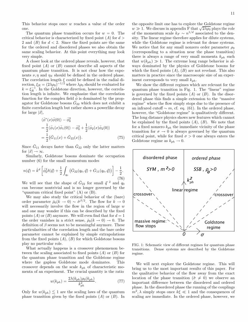
We show the different regimes which are relevant for thequantum phase transition in Fig. 1. The “linear” regimeis governed by the fixed points (A) or (B). In the disor-dered phase this finds a simple extension to the “massiveregime” where the flow simply stops due to the presence ofan infrared cutoff ∼ m, cf. eq. (61). In the ordered phase,however, the “Goldstone regime” is qualitatively different.The long distance physics shows new features which cannotbe explained by the fixed points (A), (B). We note thatfor a fixed nonzero kph the immediate vicinity of the phasetransition for σ → 0 is always governed by the quantumcritical point, while for fixed σ > 0 one always enters theGoldstone regime as kph → 0.

FIG. 1: Schematic view of different regimes for quantum phasetransitions. Dense systems are described by the Goldstoneregime.

We will next explore the Goldstone regime. This willbring us to the most important results of this paper. Forthe qualitative behavior of the flow away from the exactlocation of the phase transition (σ 6= 0) we observe animportant difference between the disordered and orderedphase. In the disordered phase the running of the couplingsm2, λ simply stops once kξ ≪ 1 and the consequences ofscaling are immediate. In the ordered phase, however, we

12

encounter the massless Goldstone fluctuations at all scales,including kξR ≪ 1. Correspondingly, the flow equations inthe regime w ≫ 1 will be nontrivial and we should exploretheir consequences.

We first work with our simplest truncation and extendit subsequently in the following sections. Within the trun-cation (15), (26) we will find a new fixed point of eq. (72)for d < 2 and a nontrivial scaling behavior for 2 < d < 3.As more couplings are included in extended truncations wefind that the fixed point persists for d = 1, while it turnsout to be an artefact of the truncation for d > 1. The pre-cise properties of the fixed point are quite sensitive to thetruncation, and the “lowest order results” of the simplesttruncation have to be interpreted with care. Indeed, for0 < d < 2 the flow equations in the ordered phase (72)exhibit an additional fixed point for w∗ 6= 0

(C) : w∗ 6= 0 , λ∗ 6= 0. (78)

The characteristic fixed point values obtained in this trun-cation by a numerical solution of eq. (72) are shown intable I. In appendix E we have performed a similar compu-tation including a local six point vertex in the truncation.Comparison of tables I and II reveals a very strong trunca-tion dependence for d near two, while the results are morerobust for d = 1.

d w∗ λ∗ η ηS t∗ d + ηS + η

1 2.257 28.3 1.73 −2.65 −8 0.08

1.9 7.33 23.8 0.335 −2.012 −80 0.23

1.99 127.3 5.85 0.021 −1.99 −500 0.021

table I: Fixed point values for (C)

Fixed point (C) is infrared attractive in all directions.Within the restricted space of couplings considered in oursimple truncation this is an example of “self-organized crit-icality”. For 0 < d < 2 the flow for any initial valuem2

Λ < 0 , λΛ > 0 will finally end in fixed point (C). In ta-ble 1 we also indicate a characteristic value of t = ln(k/Λ)

for which the fixed point is reached (for initial w and λof the order one). As d approaches two the fixed pointbehavior sets in only at extremely large distances.

Since for fixed point (C) w and λ take constant valuesone finds in the simplest truncation

ρ0(k) =w∗

2λ∗

kd

S(k), λ(k) = λ∗S(k)k2−d. (79)

With

S = S0

(k

k0

)−ηS

, A = A0

(k

k0

)−η

(80)

we infer

ρ0 ∼ kd+ηS , ρ0 ∼ kd+ηS+η,

λ ∼ k2−d−ηS , λ ∼ k2−d−ηS−2η. (81)

For ηS < −d the renormalized order parameter ρ0(k) in-creases with k, while for d + ηS + η > 0 the bare order

parameter ρ0 = A−1ρ0 vanishes for k → 0. From the val-ues of d + ηS + η in table I one would infer that no longrange order is present for d < 2. (For the one-dimensionalboson gas we find in this simple truncation that ρ0 van-ishes ∼ k0.08.) Then there is no meaningful definition ofthe critical exponent β for d = 1. Also

ξR(k) =(2λ(k)ρ0(k)

)−1/2=

1√w∗k

(82)

always diverges for k → 0, due to the existence of thefixed point for d < 2. For such a behavior there would beno meaningful definition of a correlation length even forthe radial mode, due to the strong impact of Goldstonefluctuations.

Within our simplest truncation one would conclude thatfor d = 1 a quantum phase transition exists, but the highdensity phase actually shows no long range order in a strictsense. It exhibits a powerlike decay of the correlation func-tions both for the radial and Goldstone modes. We maystill call this phase an “ordered phase” in a somewhatweaker notion: The renormalized order parameter ρ0(k)does not vanish, implying the distinction between Gold-stone and radial modes and several other features charac-teristic for an ordered phase. Also the order parameter ρ0

vanishes only asymptotically for k → 0. For a system witha characteristic infrared cutoff kph 6= 0 one can effectivelyobserve order. A similar behavior has been found [14] forclassical phase transitions, e.g. the Kosterlitz-Thouless [6]phase transition.

For d = 1 one expects for the ordered phase a behaviorsimilar to a Tomonaga-Luttinger liquid [15] with dynamicalexponent z = 1 and a correlation function

〈ϕ∗(q0, ~q)ϕ(q′0, ~q′)〉 ∼

((q0/v)2 + ~q 2

)−(1− η2 )

δ(q − q′),

〈ϕ∗(τ, ~r)ϕ(0, 0〉 ∼ (v2τ2 + ~r2)−η2 . (83)

The relativistic form of the propagator suggests that the“relativistic kinetic term” involving two ∂τ -derivativesshould not be neglected for low dimensions. We thereforewill enlarge our truncation and include the coupling V insect. VIII. This modifies the qualitative characteristics forthe flow in the Goldstone regime for d = 1, 2. For d = 2we will find that both ρ0 and ρ0 settle to constant valuesas k → 0. The fixed point (C) disappears - it is an artefactof a too simple truncation. For d = 1 we find indeed arelativistic correlation function (83) with z = 1. The flowshows again a (shifted) fixed point (C), constant w and ρ0

and λ ∼ k2 , ρ0 ∼ kη.The qualitative new features induced by the coupling

V limit the direct use of fixed point (C) in the simplesttruncation (which neglects V ). Nevertheless, the proper-ties of the flow equation (72) remain interesting in severalaspects. One concerns the “initial flow” before a substan-tial relativistic kinetic term ∼ V has been generated. Wediscuss a few details of fixed point (C) for the system (72)in appendix D.

Let us finally briefly explore the behavior of eq. (72) forlarge w - details can be found in appendix F. For d > 3

13

one finds that the flow of ρ0 and λ stops as w ∼ k−2 growsto large values for k → 0. Also the anomalous dimensionsη and ηS vanish. For d < 3 the flow of the combinationλw1/2 is attracted towards a partial fixed point. Again, theasymptotic behavior behavior for k → 0 is characterizedby constant ρ0 and A , η → 0. However, one now findsasymptotically vanishing λ ∼ S ∼ k−ηS , ηS = 2(d −3). For d < 2 an initially very large value of w decreases,consistent with the attractor property of fixed point (C).

VIII. CROSSOVER TO RELATIVISTIC MODELS

FOR LOW DIMENSIONS

For the Goldstone regime in d = 1 and d = 2 an im-portant qualitative shortcoming of our simplest truncationbecomes visible if we include the term with two time deriva-tives in an extended truncation

ΓV = −V

∫

x

φ∗∂2τφ. (84)

A nonvanishing coupling V will always be generated by theflow of Γk in the SSB regime, even if one starts with V = 0in the “classical action” at the microscopic scale Λ. Thiscontrasts with the symmetric regime, relevant for the dis-ordered phase, where an initially vanishing V remains zeroduring the flow. For d = 3 the additional coupling V in-duces quantitative changes, but for small coupling the qual-itative changes in “overall thermodynamic quantities”, likedensity, pressure, order parameter and phase diagram, aremoderate since the modifications of the infrared runningonly concern logarithms. Still, for more detailed features,like occupation numbers for small momenta, the couplingV is dominant. For the ordered phase in d = 1, 2, however,the relativistic dynamic term” (84) will dominate over theterm linear in ∂τ and radically modify basic aspects of themacroscopic properties. In the Goldstone regime the cou-pling S vanishes for k → 0 such that the flow of the effectiveaction is attracted to a (partial) fixed point with enhanced“relativistic” SO(d + 1) symmetry. This approximate rel-ativistic symmetry qualitatively changes the properties offixed point (C). For d = 1 there will be a line of fixedpoints with different ρ0, while the bare order parameter ρ0

vanishes ∼ kη. For d = 2 the fixed point (C) disappears.The flow for k → 0 will yield w → ∞ and both ρ0 and ρ0

settle at constant values, with η = 0.We emphasize that the enhanced SO(d + 1) symmetry

concerns only the leading dynamic and gradient terms forthe Goldstone mode. It is not expected to become a sym-metry of the full effective action since the Lorentz sym-metry is not compatible with Galilei symmetry for T = 0.For example, an SO(d + 1) violating term with two timederivatives for the radial mode is possible, cf. app. G.

For an initially vanishing or very small V a nonzero valueis generated by the flow equation (λ = λS−1kd−2)

∂tV = −αVS2

k2, (85)

αV =5vd

d

(1 − η

d + 2

)λw(1 +

w

2

)(1 + w)−5/2.

(Details of the computation of the flow equation for V canbe found in appendix C.) The relative importance of thekinetic terms linear or quadratic in ∂τ can be measured bythe ratio

s =S

k√

V. (86)

As long as s remains larger than one one may guess that theeffects of S could remain important. Indeed, a naive scalingcriterion for equal importance of the terms ∼ S or V isgiven by V q0 ≈ S with Sq0 ≈ k2 such that V k2 ≈ S2. Wewill argue, however, that for the Goldstone boson physicsthe relevant scale is

√2λρ0 rather than k. The effects of the

coupling V therefore become dominant for V ≫ S2/(2λρ0)or S ≪ √

w.For s → 0 the effective action shows an enhanced

SO(d + 1) symmetry, where τ ′ = τ/√

V acts like an addi-tional space coordinate. From eq. (85) it is clear that theevolution of V essentially stops for k → 0 if S decreasesfaster than k (and αV remains bounded). This will be thecase for ηS < −1, but a weaker condition will be sufficientfor an effective stop of the running of V . Indeed, from app.C we get the flow equation for s

∂ts = −(1 + ηS)s +1

2AV (s, w, λ)s3 (87)

where

lims→∞

AV = αV , lims→0 , w→∞

AV s2 ∼ λw−2. (88)

One concludes that s is driven to zero if ηS < −1. Thispresumably happens for d = 1 and d = 2. In this casethe trajectories corresponding to an enhanced SO(d + 1)-symmetry are attractive - the long distance physics be-comes effectively relativistic. For ηS > −1 large valuesof s decrease and small values increase, suggesting a par-tial fixed point s∗(λ, w). If this occurs for large s we

find s∗ ∼ λ−1/2w1/4. The relevant question for omittingthe linear dynamic term ∼ S in the Goldstone regime iss/√

w ≪ 1. This condition is reached for k → 0 if V andS/λ go to constants, while S goes to zero. Constant valuesof V and S/λ are suggested also on physical grounds sincethese quantities correspond to thermodynamic observables,see eq. (G.27) in app. G.

In this context we note that S = 0 is always a (partial)fixed point, due to an enhanced discrete symmetry τ → −τ(while keeping φ fixed). (This additional discrete symme-try is preserved by our cutoff Rk(16), even though this cut-off does not respect the SO(d + 1) symmetry - see app. Cfor a discussion on this issue.) For ηS < −1 the fixed pointat s = 0 is IR-attractive, while for ηS > −1 it becomes re-pulsive. For d = 3, where ηS > −1, the flow therefore endsfor k → 0 with nonzero s, corresponding to a violation ofSO(d + 1) symmetry in the radial sector. For d = 3 oneexpects that V stops running for k → 0 due to w → ∞.For large w one finds in eq. (85) αV = (λ/2ρ0)

1/2k2/Sand ∂tV ∼ S ∼ (ln k0/k)−1. For λ/S → const we thereforehave logarithmic behavior

λ ∼ S ∼ 1

ln(k0/k)(89)

14

and we note the difference as compared to the simplesttruncation (F.7), where λ decreases with the square ofthe inverse logarithm. This implies that s diverges ∼k−1 ln(k0/k) such that for d = 3 the large s regime ap-plies.

Also for d = 1, 2 the running of V stops, this time dueto SO(d + 1) symmetry. The running of ρ0 and λ withinthe Goldstone regime in the relativistic models has beenintensively studied by non-perturbative flow equations [22],[10]. For w → ∞ the running of ρ0 stops. On the otherhand, the fluctuations of the Goldstone modes produce afixed point for the dimensionless coupling λkd−3 for all d <3. One infers for the effective momentum dependence of thequartic coupling

λ(~q2) ∼ (~q2)3−d2 . (90)

Comparison with the simplest truncation (F.14) shows thatηS has to be replaced by d − 3 instead of 2(d − 3). Thisunderlines again the crucial importance of the relativistickinetic term for the long distance physics in all dimensiond ≤ 3.

The summary of the situation in the Goldstone regimeis rather simple. For all d the asymptotic value for Vreaches a constant as k → 0. For d = 3 also S becomes al-most constant (it vanishes only logarithmically), whereasfor d = 1 and d = 2 the flow rapidly approaches an en-hanced SO(d + 1)-symmetry due to S vanishing with apower law S ∼ k−ηS , S/k → 0. The value of the renormal-ized order parameter ρ0 approaches a constant for d ≥ 1.For d > 1 the anomalous dimension η vanishes for w → ∞and also ρ0 become constant. The renormalized quarticcoupling shows a scaling behavior according to its canoni-cal dimension in the relativistic model.

For d = 1 and d = 2 the consequences of the “relativis-tic asymptotics” are immediate - the Goldstone regime isdescribed by the classical O(2)-model in d + 1 dimensions.

With τ ′ = τ/√

V , q′0 = q0

√V the correlation function for

large distances in space and time (or small momenta ~q, q0)obey

(G = (G11 + G22)/2)

G ∼ (~q 2 + q′20 )−1 , G ∼ (~q 2 + q′20 )−1+η/2,

G ∼ (~r 2 + τ ′ 2)1−d2 , G ∼ (~r 2 + τ ′2)

1−d−η2 . (91)

(We recall that G is dominated by the Goldstone contribu-tion.) One may generalize the concept of dynamical crit-ical exponent also for situations without a finite correla-tion length. For d = 1, 2 the effective dynamical criticalexponent takes the “relativistic value” z = 1. For d = 2the Goldstone regime is described by the three-dimensionalclassical model. It is well known that ρ0 and ρ0 settle toconstants, with η(k → 0) = 0.

At this point we can already extend our discussion to anarbitrary number M of complex fields. The potential u(ρ),the gradient term and the relativistic dynamical term ∼ Vall obey an extended O(2M)-symmetry. For our trunca-tion, the asymptotic behavior for the flow equations in theSSB regime is therefore well known for d = 1 and d = 2.Since S vanishes asymptotically, and S is the only term

in our truncation that violates the O(2M) symmetry, theasymptotic behavior of the flow is given by the classicalO(2M)-models in d + 1 dimensions. (A more general dis-cussion of M -component models will be given in sect. X.)In particular, for d = 2 one finds a simple description oforder for arbitrary M in terms of the three-dimensionalclassical O(2M) models.

For d = 1 the two dimensional classical model applies.By virtue of the Mermin-Wagner theorem we know thatno long range order exists with a spontaneously brokencontinuous symmetry. Since any ρ0 6= 0 would lead tospontaneous breaking of the U(1)-symmetry we can con-clude ρ0(k → 0) = 0. The way how the Mermin-Wagnertheorem is realized depends on the number of componentsM [9]. For M > 1 both ρ0(k) and ρ0(k) reach zero at somepositive value kSR. For kph < kSR no order persists, whilefor kph > kSR the system behaves effectively as in the pres-ence of order. Typically, ordered domains exist with sizeLd . k−1

SR. Since the running of ρ0 is only logarithmic thescale kSR can be exponentially small. For an experimentalprobe with size L one has kph > L−1 so that for practicalapplications an “ordered phase” will persist. The typicalsize of ordered domains is then larger than the size of thesystem. (This issue has been discussed in detail for classicalantiferromagnetism in two dimensions [23].)

For M = 1, in contrast, ρ0 reaches a constant value fork → 0. Only the bare order parameter vanishes due toa nonvanishing anomalous dimension, ρ0 ∼ kη, such thatorder does not exist in a strict sense. In the correspond-ing classical model this situation describes the “low tem-perature phase” related to the Kosterlitz-Thouless phasetransition. For practical purposes this phase behaves likean ordered phase, with powerlike decay of the correlationfunction G (91) due to the existence of a Goldstone boson.This is also the characteristic behavior of a Tomonaga-Luttinger liquid. It is well known from the classical O(2)model in two dimensions that the low temperature phaseis characterized by a line of fixed points which may belabelled by ρ0 = ρ0(k → 0). The anomalous dimensiondepends on ρ0 [9, 14]

η =1

4π√

V ρ0

. (92)

It seems plausible that ρ0 depends on the effective chemicalpotential σ such that we predict an anomalous dimensiondepending on σ.

It is remarkable that the main qualitative features ford = 1 and k → 0, namely a nonzero ρ0, vanishing ρ0, anda positive anomalous dimension η > 0, are already visi-ble from fixed point (C) in the simple truncation of sect.VI. Not surprisingly, however, the quantitative accuracyfor the anomalous dimensions is very poor if the couplingV is omitted. We may indeed address the properties of theGoldstone regime in the perspective of the properties offixed points in presence of the coupling V . For d = 2 onehas the well known Wilson-Fisher fixed point of the threedimensional classical model. It corresponds to S = 0. Thequestion of how close trajectories approach the Wilson-Fisher fixed point depends on the microscopic parameters σ

15

and λΛ as well as on a possible microscopic coupling V (Λ).Quantum phase transitions with critical behavior differentfrom eq. (52) can be associated with the Wilson-Fisherfixed point. In this case z = 1 and the critical exponentsν and η of the three-dimensional O(2M) model apply. Ford = 2 this type of phase transition presumably becomesrelevant for large enough microscopic couplings V (Λ). ForV (Λ) = 0, as considered in this paper, the quantum criticalfixed point discussed in sect. V is relevant. For this quan-tum critical fixed point a vanishing relativistic couplingV = 0 is stable with respect to the flow. In our truncationwe infer from eq. (85) that for w = 0 one has αV = 0 andtherefore ∂tV = 0 while there is anyhow no contribution to∂tV in the disordered phase. At the quantum critical pointthe dimensionless combination V k2 therefore correspondsto an irrelevant coupling.

In order to judge the relevative importance of theWilson-Fisher (WF) and the quantum critical (QC) fixedpoints for arbitrary microscopic couplings V (Λ) one shouldconsider the critical hypersurface on which both fixedpoints lie. (Note that ρ0(Λ) varies on this hypersurface,with ρ0(Λ) = 0 for QC and ρ0(Λ) > 0 for WF. We use acommon name (QC) for fixed point (A) (d > 2) or fixedpoint (B) (d < 2)). The first question concerns the sta-bility of WF with respect to the coupling S. Taking intoaccount the scaling dimensions at WF one finds that WF isstable for ηS < −1 and unstable for ηS > −1. Here ηS hasto be evaluated for WF, which we have not done so far. ForηS > −1 one would observe a crossover from WF to QCon the critical hyperface. In contrast, for ηS < −1 bothWF and QC are stable on the critical hypersurface. Thetopology of the flow would then imply the existence of anew fixed point with finite nonzero value of S(Λ)/

√V (Λ).

For d = 1 (and M = 1) the role of the Wilson-Fisherfixed point is replaced by the Kosterlitz-Thouless fixedpoint for the two dimensional classical O(2) model. Akey new ingredient is the existence of a whole line of fixedpoints for S = 0. They can be parameterized by the renor-malized order parameter ρ0 (corresponding to κ in Ref. [14]at k = 0. These fixed points govern the Goldstone regimeof our model with V (Λ) = 0. Thus the IR attractive fixedpoint (C) in the truncation with V = 0 transforms into oneof the fixed points on the critical line. Now w is no longeran irrelevant coupling - it can be used to parameterize theline of fixed points instead of ρ0. (Indeed, w = 2(λ/k2)ρ0

and (λ/k2) approaches a fixed point value depending on ρ0

[9].) It seems natural that ρ0 depends on σ. On the otherhand, ρ0(k = 0) cannot take arbitrary small values, corre-sponding to the jump in the renormalized superfluid den-sity of the Kosterlitz-Thouless transition [24]. This raisesinteresting questions of how the chemical potential σ ismapped into an allowed range of ρ0 or w. It is likely thatthe answer is linked to the “initial flow” for small V witha possible influence of an approximate fixed point of type(C) for which V is a small perturbation.

We observe that on the line of fixed points the anomalousdimension η depends on ρ0. The maximal value η = 1/4 isreached at the Kosterlitz-Thouless transition. Our trunca-tion therefore predicts η ≤ 1/4 for eq. (91), and we infer

for d = 1 , M = 1

G ∼ (r2 + τ ′2)−η2 . (93)

However, it is known for the Tomonaga-Luttinger liquidthat the maximal value for η is 1/2. This brings us to thequestion of reliability of a truncation that only includes apotential, second order gradient terms and first and secondorder time derivatives with SO(d+1) symmetry for S = 0.For V > 0 such a truncation is not compatible with Galileiinvariance for T = 0 and ρ → 0. We conclude that thedescription in terms of a d+1-dimensional O(2) model be-comes problematic for w . 1. On the other hand we havepresented strong arguments for its validity for w ≫ 1. Weconclude that the identification of the Tomonaga-Luttingerliquid with the Kosterlitz-Thouless phase of the two di-mensional model may only be valid for large w. For w ≈ 1certain terms neglected in our tuncation and breaking ofthe SO(d + 1) symmetry can play a role. The range of ηnear 1/4 in the two-dimensional O(2) model corresponds tow ≈ 1 - this is the region of the phase transition. We con-clude that our approximation is expected to hold as longas η is small enough (large w), but may break down for ηnear 1/4, such that the upper bound η ≤ 1/4 is not robust.

We finally comment on the case d = 3 where the lin-ear τ -derivative remains important, as far as naive scalingis concerned. However, in the Goldstone regime the lin-ear τ derivative involves the radial mode ϕ1,

∫ϕ∗∂τϕ ∼∫

ϕ1∂τϕ2. If we study the long range physics the radialmode effectively decouples for distances larger than the cor-relation length and we should question the criterion s . 1that we have used for an estimate of the importance of theterm ∼ V . This criterion is valid for physics involving theradial mode, i.e. kph & ξ−1

R . We will discuss in the next

section that for kph ≪ ξ−1R the relevant dimensionless ratio

is not given by s but rather by S/√

2λρ0V . This can beseen by “integrating out” the radial mode and investigat-ing the effect of S in a nonlinear model for the Goldstoneboson.

IX. GOLDSTONE REGIME AND NON-LINEAR

σ-MODELS

In the Goldstone regime the influence of the radial modeis subdominant. We may therefore aim for a descriptiononly in terms of Goldstone bosons. This leads to the non-linear σ-models. The effective action in the nonlinear for-mulation can directly be computed from our results. Onesolves the field equation for the radial fluctuations as afunctional of the Goldstone fluctuations and reinserts thissolution into the effective action. For this purpose we pa-rameterize

φ(x) =(φ0 + R(x)

)eiθ(x) (94)

and eliminate the radial mode R(x) as a functional of theperiodic phase variable θ(x).

Within our truncation

S =

∫

x

L , L = u(φ∗φ) + Sφ∗∂τφ − φ∗(∆ + V ∂2τ )φ (95)

16

we find (for constant S, V and removing total derivativesand constants)

L = L0 + LR,

L0 = φ20~∇θ~∇θ + V ∂τθ∂τθ,

LR = u(φ20 + 2φ0R + R2) − u(φ2

0)

+(2φ0R + R2)~∇θ~∇θ + V ∂τθ∂τθ + iS∂τθ+~∇R~∇R + V ∂τR∂τR. (96)

The field equation δLR/δR = 0 can be solved iteratively

by expanding in ~∇θ~∇θ + V ∂τθ∂τθ + iS∂τθ. In lowestorder one obtains, with λ = u′′(φ2

0),

R = −φ0(2λφ20−∆−V 2∂2

τ )−1~∇θ~∇θ+V ∂τθ∂τθ+ iS∂τθ,(97)

and reinserting this solution yields (ρ0 = φ20)

LR = −ρ0iS∂τθ − V ∂τθ∂τθ − ~∇θ~∇θ (98)

(2λρ0 − ∆ − V ∂2τ )−1iS∂τθ − V ∂τθ∂τθ − ~∇θ~∇θ.

Expanding in powers of θ

LR = LR,2 + Lint,

LR,2 = ρ0S2∂τθ(2λρ0 − ∆ − V ∂2

τ )−1∂τθ (99)

and combining with L0 we obtain the effective inverse prop-agator for the Goldstone boson (∼ φ0θ)

G−1g = ~q 2 + V q2

0 +S2q2

0

2λρ0 + ~q 2 + V q20

. (100)

On the other hand, Lint contains interaction terms. Theseare purely derivative interactions, as appropriate for Gold-stone bosons. Higher orders in the iterative expansion willonly yield further interaction terms.

The inverse Goldstone propagator shows no term linearin q0, even for V = 0 , S = 1. This is a simple consequenceof the observation that a linear τ -derivative for a singlereal field is always a total derivative and can therefore beeliminated from the field equations. In lowest order in aderivative expansion (for small momenta) one has

Gg =

[~q 2 +

(V +

S2

2λρ0

)q20

]−1

(101)

such that both V and S contribute to an effectively rel-ativistic kinetic term. (In the limit of large q0 , V q2

0 ≫2λρ0 + ~q 2, the correction from LR results in an effectivemasslike term S2/V , i.e. Gg = [~q 2 + V q2

0 + S2/V ]−1.) Asmentioned at the end of the preceeding section the relevantratio for the importance of the linear dynamic term ∼ S isgiven for the Goldstone regime by S/

√2λρ0V .

We conclude that in the Goldstone regime the renormal-ized propagator always takes a relativistic form

Gg =[~q 2 + (q0/v)2

]−1. (102)

The quantity

v2 =

(V +

S2

2λρ0

)−1

(103)

can be associated with the microscopic sound velocityof the Goldstone mode. Comparing with eq. (G.23)in appendix G we see that it equals the macroscopicsound velocity, cs in accordance with Ref. [3]. Forρ0 → const, S/λ → const, S → 0, the second termin eq. (103) can be neglected. This yields a simple relationbetween the sound velocity and the coupling V = V (k → 0)

c2s = V −1. (104)

The bare propagator reads correspondingly

Gg =[~q 2 + (q0/v)2

]−(1− η2 )

(105)

where η depends on momenta according to the replacementk2 → ~q 2 + q2

0/v2. For d > 1 the anomalous dimension van-ishes asymptotically, η(k → 0) = 0. The generalization toM component fields is straightforward and will briefly beaddressed in the next section. We emphasize that for thenonlinear models the propagator shows no qualitative dif-ference between a linear dynamic term ∼ S or a relativisticdynamic term ∼ V . Nevertheless, the form of the dynamicterm becomes important for the linear model, in particularfor the flow of the order parameter ρ0(k).

X. M-COMPONENT MODELS

For models with a relativistic kinetic term the critical ex-ponents depend sensitively on the number of componentsof the field. For N real components and scalar modelswith O(N) symmetry the universality classes can be fullycharacterized by N and d. We may investigate this ques-tion also for the nonrelativistic kinetic term and investigatemodels with M complex scalar fields φm , m = 1 . . .M .In terms of renormalized fields we consider models withU(M)-symmetry and neglect first the coupling V

Γk =

∫

x

∑

m

(Sφ∗m∂τφm − φ∗

m∆φm) + u(ρ). (106)

Due to the U(M) symmetry the potential can only dependon the invariant ρ =

∑m

φ∗mφm. Since ρ is invariant with

respect to the symmetry O(2M) acting on the 2M realcomponents of the scalar field, the potential exhibits anenhanced O(2M) symmetry. This enhanced symmetry isshared by the term involving spatial gradients but violatedby the linear τ -derivative.

Within our truncation of pointlike interactions and witha linear τ -derivative, we find a very simple result: the flowequations do not depend on M , except for the flow of a fieldindependent constant in u. Neglecting the momentum de-pendence of interactions all our discussion therefore holdswithout modifications for the M -component case as well.As long as the propagator is specified by eq. (106) a de-pendence of the critical exponents on M can therefore onlyarise from the momentum dependence of the interactions.This situation is quite different in presence of a relativistickinetic term involving two τ -derivatives.

17

In order to show this result we first note that for a con-stant background field the inverse propagator is block di-agonal, G−1= diag(G−1

1 , G−12 . . . ) where G−1

m are 2 × 2matrices corresponding to a decomposition of the complexfield φm into real and imaginary parts. Without loss ofgenerality we may take a real constant background fieldin the m = 1-direction. Then G−2

1 is given by eq. (20)whereas for m > 1 one has

G−1m 6=1 =

(q2 + u′ , −Sq0

Sq0 , q2 + u′

). (107)

The resulting correction to ∂tu from the (M−1) additionalcomponents does not depend on ρ

∆∂tu|φ =4(M − 1)vd

dSkd+2

(1 − η

d + 2

). (108)

A field independent additive constant does not influenceour discussion and we recover the same flow equations forw and λ as for M = 1.

We next turn to the computation of η and ηS . We definethese quantities by the flow of the ~q 2 and q0 dependenceof the inverse propagator for the m = 1 component, ac-cording to eqs. (35), (36). We can use eqs. (30), (31) withindices a, b . . . , running now from 1 to 2M , e.g. the m = 2component corresponds to a = 3, 4 etc.. In presence of abackground field in the a = 1 direction the interaction termin the effective action for the fields φb, b 6= 1 has a discretesymmetry φb → −φb. This implies that for nonvanishingcubic couplings γacd the values of all indices must appearin pairs, except for the value one. For the anomalous di-mension η the indices a and b in eq. (31) take the valuetwo. In consequence, the index pair (d,e) can only be (1,2)or (2,1), and similar for the index pair (f, c). Therefore noindices c, d, e, f with values three or higher appear and theadditional (M − 1) complex fields do not influence η. ForηS the situation is similar if one also uses the fact that Gis block diagonal, i.e. G1,b>2 = G2,b>2 = 0. (The situa-tion can be easily depicted in terms of one-loop Feynmangraphs with two external legs.) This closes our argumentthat the flow equations are independent of the number ofcomponents M in the approximation of pointlike verticesand for V = 0.

We conclude that the symmetric phase and the quan-tum phase transition are not influenced by the presenceof additional components of the field. At the quantumcritical point one finds for all M the critical exponentsν = 1/2 , η = 0 , z = 2. In the ordered phase the numberof components will influence the flow as soon as a sizeablestrength V for the second τ -derivative is generated. In par-ticular, the flow for d = 1 and d = 2 will depend on M .The flow for k → 0 is expected to reproduce the well knownbehavior of the Goldstone boson physics in classical statis-tical systems [8, 9, 10]. Typically, the asymptotic behaviorcan be described by nonlinear σ-models on a manifold givenby the coset space U(M)/U(M − 1). For d +1 = 2 the be-havior of the abelian model for M = 1 differs substantiallyfrom the non-abelian σ-models for M > 1.

In the microscopic action only the coupling S violatesthe O(2M) symmetry. In analogy, we expect that forsmall O(2M) violating couplings, i.e. small S we canchoose a description in terms of O(2M)/O(2M−1)-models.This will contain symmetry breaking effects since theO(2M) symmetry is exact only for S = 0. Such ef-fects are proportional to the dimensionless combinationS(k)/(

√2λ(k)ρ0(k)V (k)). Since for d = 1, 2 the flow is

attracted towards S = 0 (if ηS < 0), one may suspect thatthe enhanced symmetry for S = 0, i.e. the space-time ro-tations SO(d + 1) and the internal rotations SO(2M), areapproximately realized in the Goldstone regime. The de-gree of violation of these symmetries depends on the char-acteristic momentum scale of the Green’s functions and onw−1. As before, a nonzero “external momentum” ~q maybe associated with k2

ph = ~q 2 > 0. Since S(k) vanishesonly asymptotically for k → 0 the symmetry breaking ofSO(d + 1) and SO(2M) due to S(kph) > 0 will always bepresent. Furthermore, the vanishing of S occurs for largew, while S remains important for w . 1.

The order parameter ρ0 or ρ0 is a quantity that in-volves the limit of zero momentum (or kph ≈ L−1 withL the macroscopic size of the probe). We may there-fore take the limit k → 0 , ~q 2 → 0 for the issue ofspontaneous symmetry breaking. For small momenta wemay consider a derivative expansion of the effective ac-tion (for k → 0). Let us consider up to two derivatives.For 1 < d ≤ 2 both w−1 and the ratio S(k)/k vanish fork → 0 and s can be neglected. The potential and the rela-tivistic two-derivative term −φ∗(V ∂τ2 + ∆)φ respect both

SO(d + 1) and O(2M). A term ∼ −Y ρ(V ∂τ2 + ∆)ρ vio-

lates SO(d + 1) only if V 6= V , while it preserves O(2M).On the level of two derivatives an O(2M) violation couldonly arise from a term

∫x(ϕ∗

1ϕ1∂τϕ∗2∂τϕ2 +ϕ∗

2ϕ2∂τϕ∗1∂τϕ1

−ϕ∗2ϕ1∂τϕ∗

1∂τϕ2 − ϕ∗1ϕ2∂τϕ∗

2∂τϕ1) for M = 2, or suitablegeneralizations for M > 2. (On the level of two derivativesthe invariants preserving U(M) while violating O(2M) areof the form |ǫm1...mN

φm1. . . φmN−1

∂φmN|2.)

For d = 2 we may speculate that the SO(d + 1) andO(2M) violating terms involving two derivatives vanish fork → 0. The behavior of the order parameter and the corre-lation function at small momentum are then well approxi-mated by the classical O(2M) model in three dimensions.This issue depends on whether the Lorentz symmetry vi-olating operators are irrelevant for the trajectories withw → ∞, or not. Even in presence of O(2M) violatingderivative terms one would still find 2M − 1 gapless ex-citations, due to the accidental O(2M) symmetry of thepotential.

For d = 1 the issue may be more complicated. Withinthe relativistic model w is either constant (for M = 1)or runs logarithmically towards zero (M > 1). We maytherefore encounter a region where w . 1 such that theSO(d + 1) violating terms can no longer be neglected. ForM > 1 this region becomes always relevant for k → 0.For M = 1 we expect that SO(d + 1)-symmetry becomesa good approximation for the fixed points with small η(large w), whereas it is questionable for the larger valuesof η corresponding to w ≈ 1.

18

XI. CONCLUSIONS AND OUTLOOK

The functional renormalization group yields a unifiedpicture for quantum phase transitions of bosons. It coversboth the ordered and the disordered phase, including therather complicated long range dynamics of the second. Wedescribe within the same simple truncation an arbitrarynumber of space-dimensions d and an arbitrary numberof components M (for M complex fields with symmetryU(M)). In a general setting, the properties of the phasetransition depend on the parameter sΛ which characterizesthe relative strength of the kinetic terms involving one ortwo time derivatives. More precisely, for a general micro-scopic (or classical) action (1) the dimensionless ratio sΛ isgiven by

sΛ =S

Λ

√2MB

V=

S(Λ)

Λ√

V (Λ), (109)

with Λ the ultraviolet cutoff.The characteristic features are described by two limits.

The point sΛ = 0 describes models with a “relativistickinetic” term involving two time derivatives and an en-hanced space-time symmetry SO(d + 1). For those modelsthe quantum phase transition in d dimensions is strictlyequivalent to the classical phase transition in d + 1 dimen-sions. The universal critical properties correspond to thewell studied O(2M)-models in d + 1 dimensions.

For the other limit sΛ → ∞ (i.e. V = 0) Galilei symme-try characterizes the zero temperature physics. Now thephase transition is influenced by the non-relativistic quan-tum critical point. This is the case we have mainly studiedin this paper. For intermediate values of sΛ one expectsnear the phase transition a crossover from the “classical”or “relativistic” critical point to the non-relativistic quan-tum critical point. No phase transition is expected as sΛ isvaried. However, the critical exponents and amplitudes willdepend on sΛ. They are given by the universality class ofthe d+1 dimensional relativistic O(2M) models in the limitof small sΛ - for example by the well known Wilson-Fishercritical point for d = 2. As sΛ increases towards infinitythe critical exponents smoothly change towards the meanfield values for the non-relativistic quantum critical point.We note that for sΛ 6= 0 the critical hypersurface for thephase transition typically occurs for nonzero density.

The critical behavior for the nonrelativistic “quantumcritical models”(i.e. sΛ → ∞) can be characterized by tworegimes, depending on l/D. Here l is a characteristic lengthscale of the system or experiment, and D is proportional tothe average distance between (quasi-) particles, D ∼ n−1/d.The “dilute regime” applies to the disordered phase (whereD → ∞) and to the “linear regime” in the ordered phase,as shown in fig. 1. In the dilute regime simple scaling lawsapply and the critical behavior is described by mean fieldcritical exponents for all d and M . The simplicity of itsproperties finds a simple explanation, since the disorderedphase describes the vacuum with zero particles, and for thelinear regime in the ordered phase the small density givesonly subleading corrections. In more technical terms, thisis the regime where k2

ph = l−2 ≪ 2λρ0 or w ≪ 1.

For l ≫ D the particle density matters. For this “denseregime” the particle density n sets a new relevant mo-mentum scale ∼ D−1 or energy scale (2MBD2)−1. Thelong distance physics is described by the interacting Gold-stone bosons which arise from the spontaneous breaking ofU(M)-symmetry. We therefore often call the dense regimethe “Goldstone regime”. Since Goldstone bosons must bemassless (or “gapless”) the correlation functions decay withan inverse power of distance in space or time.

The physics of interacting Goldstone bosons crucially de-pends on the number of space dimensions d. For d = 3 wefind that the “Goldstone dynamics” is influenced both byshort and long wave length fluctuations. The running ofdimensionless couplings is logarithmic. For small or mod-erate interaction strength λΛ mean field theory remains agood guide. Quantum corrections induce quantitative cor-rections but do not change the qualitative behavior, exceptfor the extreme infrared. We do not address in this paperthe possibility that large λΛ may lead to new phenomena,as the destruction of the condensate by a too large repul-sion between the bosons.

On the other hand, for d = 2 and d = 1 the Goldstone dy-namics is infrared dominated, leading to qualitatively newfeatures induced by quantum fluctuations. One expectsstrong deviations from mean field theory. We find that therenormalization flow describes a crossover to models witha relativistic kinetic term. Even for models with sΛ → ∞(i.e. V = 0) the value of s(k) decreases fast for momentumscales k ≪ Λ. The relativistic term ∼ V will be induced bythe fluctuations and dominates for k → 0. The Goldstoneregime for d = 1, 2 is therefore characterized by s = 0, bothfor sΛ → ∞ and for sΛ = 0. In other words, the flow isattracted fast towards the (partial) fixed point s = 0. (Theflow in the Goldstone regime differs from the flow on thecritical hypersurface where s presumably diverges.)

This implies for d = 1, 2 a close link between the Gold-stone regime of the quantum model in d dimensions andthe corresponding Goldstone regime of the classical modelin d + 1 dimensions. The classical Goldstone regime iswell studied. For d = 2 one expects a description of theGoldstone regime by the classical three-dimensional U(M)-model. In this case the realization of order is straightfor-ward, with both ρ0 and ρ0 approaching constants for k → 0and η tending to zero. The correlation function for largeseparations in space or time shows a simple powerlike be-havior

G(q) ∼ G(q) ∼ (~q 2 + q20/c2

s)−1,

G(x) ∼ G(x) ∼ (~r 2 + c2sτ

2)−1/2. (110)

Here we have restored dimensions, with sound velocity cs =v/(2MB).

For d = 1 the “ordered phase ” actually shows no longrange order in a strict sense. The influence of the Goldstonebosons is so strong that they destroy any long range order.This agrees with the Mermin-Wagner theorem for the clas-sical two-dimensional models with continuous global sym-metry, as applicable here. The way how this theorem isrealized depends crucially on M . For M = 1 the non-linear

19

σ-model is abelian. In the ordered phase the relevant ex-citations include vortices. Indeed, the Kosterlitz-Thoulessphase transition finds within the functional renormaliza-tion group a simple description in terms of a linear O(2)model in two dimensions [14]. As a result, the renormalizedorder parameter ρ0 reaches a constant for k → 0, while thebare order parameter ρ0 vanishes ∼ kη due to a nonvanish-ing anomalous dimension. The correlation function decaysas

G(q) ∼ (~q 2 + q20/c2

s)−(1−η

2 ),

G(x) ∼ (~r 2 + c2sτ

2)−η2 . (111)

These findings carry over to the non-relativistic model ford = 1, the Tomonaga-Luttinger liquid. In our approach thekey features of the Tomonaga-Luttinger liquid result essen-tially from the nonzero value of the renormalized order pa-rameter ρ0. This model simply describes the Goldstone bo-son associated to the “effective U(1) symmetry breaking”.The anomalous dimension depends on the density of quasi-particles, n = ρ0. For large κ =

√V n = n/v = n/(2MBcs)

one finds from eq. (92)

η =MBcs

2πn. (112)

After restoring dimensions the sound velocity cs is relatedto the coupling V by eq. (G.27)

c2s =

1

4M2BV

. (113)

For M > 1, as for example for the ferromagnetic to para-magnetic transition with M = 3, the nonlinear σ-modelsare asymptotically free and induce a nonperturbative scalekSR. Within a description by linear U(M) models one findsthat ρ0(k) and ρ0(k) both vanish for k = kSR, while be-ing finite for k > kSR. For k < kSR the flow follows thesymmetric regime with a minimum of the potential at theorigin. The situation with nonzero ρ0(k) describes localorder, with a maximal size of domains up to k−1

SR. Theorder in larger domains is destroyed by the Goldstone bo-son fluctuations. Since kSR can be exponentially small forlarge enough density (the running of ρ0(k) is only logarith-mic), there is always a critical density nc beyond which thesize of ordered domains k−1

SR grows beyond the macroscopicsize of the experimental probe L. Thus for n > nc one ob-serves effectively spontaneous symmetry breaking, despitethe Mermin-Wagner theorem.

The dynamical behavior of the quantum critical modelscan be characterized by a dynamical critical exponent z. Ingeneral terms, it describes how a characteristic time scaleτ scales with a characteristic length l, i.e. τ ∼ lz. Wehave concentrated on the non-relativistic quantum criticalmodels (sΛ → ∞). We find for all d and M that thevalue of z depends on the density of (quasi)-particles. Forthe dilute regime one has the mean field scaling z = 2,while the dense regime shows the relativistic value z = 1.Inbetween, there is an effective crossover. As far as timescales are concerned the Goldstone regime (dense regime)

applies for τ > D/cs, with D the interparticle distance∼ n−1/d and cs the sound velocity.

This paper has demonstrated that the flow of a smallset couplings, namely ρ0 (or m2), λ, S and V yields allqualitative features for the quantum phase transition forarbitrary d and M . The quantitative precision can be im-proved by extending the truncation. Straightforward stepsinclude the incorporation of a nonvanishing V in the flowequations for the effective potential u and for ηS , as wellas a differentiation between the effective renormalizationconstants for the radial and Goldstone modes via the in-clusion of a term ∼ Y ∂ρ∂ρ. Together with γ = u(3)(ρ0) weexpect that the set of couplings (ρ0, λ, γ, S, V, Y ) will yieldalready a very satisfactory quantitative accuracy. Exten-sions to include fermionic degrees of freedom are possible[25]. Furthermore, the effects of nonvanishing temperaturecan easily be incorporated in our framework - one sim-ply has to replace the q0-integration by a Matsubara sum.Close to the critical temperature of the phase transitionand away from the quantum critical point at T = 0 theflow will experience an effective dimensional reduction tothe classical d-dimensional U(M) models. High accuracyfor the functional flow equations has already been reachedfor the classical O(N) models in arbitrary dimension. In-cluding the temperature effects the flow equations shouldprovide a rather complete picture for the thermodynamicsof bosonic quantum gases.

In this paper we have concentrated on the structuralaspects. A numerical solution of the flow equations for k →0 will directly yield important thermodynamic quantitiesin the zero temperature limit. The density is given byn = ρ0 and the condensate fraction by Ωc = A−1. Thesound velocity obeys cs = 1/(2MB

√V ) for d = 1, 2, with

logarithmic corrections for d = 3 due to S ∼ 1/ ln(k0/k),cf. app. G,

c2s =

1

4M2BV

[1 − S

(1 +

∂ ln Ωc

∂ lnn

)]. (114)

The change of the condensate fraction with the densityfollows (cf. app. G)

∂ ln Ωc

∂ lnn=

2M2Bc2

sS

λn− 1 → S

2λρ0V− 1, (115)

with λ the renormalized quartic coupling.

It may be possible to measure all these quantities byinvestigating the Bose-Einstein condensate for ultracoldbosonic atoms. With suitable traps one may prepare essen-tially homogeneous systems for d = 1, 2 or 3. For a quanti-tative computation one will further need to determine λΛ

in dependence on external parameters, as a homogeneousmagnetic field. For this purpose one relates it to measur-able properties in the vacuum, like the scattering length ford = 3. The necessary computation for n = 0 correspondsprecisely to the phase transition discussed in sect. V andcan be performed in the comparatively simple disorderedphase. The prospects for experimental tests of some of thefeatures described in this paper look promising.

20

Note added:

After the first version of the paper interesting extensionsand numerical results have been obtained in Ref. [26].

Acknowledgment:

The author would like to thank S. Diehl, S. Floerchinger, H.Gies, J. Pawlowski and M. Scherrer for fruitful discussionand collaboration.

APPENDIX A: Flow equation for the effective

potential

We can write the flow at fixed renormalized field φ

∂tu = ηρu′ (A.1)

+

∫

q

[k2 − η

2(k2 − ~q 2)

]θ(k2 − ~q 2)trG

= ηρu′ + 8vd

k∫

0

dqqd−1[k2 − η

2(k2 − q2)

]g,

where v−11 = 4π, v−1

2 = 8π, v−13 = 8π2 and q = (~q 2)1/2.

The integration over q0 can be carried out easily

g =1

2

∫dq0

2πtrG

=

∫dq0

(2π)

q2 + u′ + ρu′′

S2q20 + (q2 + u′)(q2 + u′ + 2ρu′′)

=1

2S

q2 + u′ + ρu′′√

q2 + u′√

q2 + u′ + 2ρu′′. (A.2)

In the integrand we can use q2 = k2 such that the q inte-gration is trivial and yields eq. (22).

Differentiation of eq. (22) with respect to ρ yields

∂tu′ = η(u′ + ρu′′)

−2vd

dSkd+2

(1 − η

d + 2

)

1√k2 + u′

1√k2 + u′ + 2ρu′′

ρu

′′2

k2 + u′ −3ρu

′′2 + 2ρ2u′′u(3)

k2 + u′ + 2ρu′′

. (A.3)

The second derivative reads

∂tu′′ = η(2u′′ + ρu(3))

−2vd

dSkd+2

(1 − η

d + 2

)

1√k2 + u′

1√k2 + u′ + 2ρu′′

u

′′2 + 2ρu′′u(3)

k2 + u′ (A.4)

−3u′′2 + 10ρu′′u(3) + 2ρ2(u(3)2 + u′′u(4))

k2 + u′ + 2ρu′′

−3

2ρu′′

[u

′′2

(k2 + u′)2− (3u′′ + 2ρu(3))2

(k2 + u′ + 2ρu′′)2

]

while the third derivative becomes already quite lengthy

∂tu(3) = η(3u(3) + ρu(4))

−2vd

dS

(1 − η

d + 2

)kd+2

1√k2 + u′

1√k2 + u′ + 2ρu′′

R (A.5)

with

R =X1

k2 + u′ −X2

k + u′ + 2ρu′′

− Y1

(k2 + u′)2+

Y2

(k2 + u′)(k2 + u′ + 2ρu′′)

+Y3

(k2 + u′ + 2ρu′′)2

+Z1

(k2 + u′)3+

Z2

(k2 + u′)2(k2 + u′ + 2ρu′′)

− Z3

(k2 + u′)(k2 + u′ + 2ρu′′)2

− Z4

(k2 + u′ + 2ρu′′)3(A.6)

and

X1 = 4u′′u(3) + 2ρ(u(3)2 + u′′u(4)),

X2 = 16u′′u(3) + 14ρ(u(3)2 + u′′u(4))

+2ρ2(3u(3)u(4) + u′′u(5)),

Y1 = 3u′′2(u′′ +5

2ρu(3)),

Y2 = ρu′′(u′′u(3) − ρu(3)2 + ρu′′u(4))

Y3 = (3u′′ + 2ρu(3))(9u′′2 +75

2ρu′′u(3)

+6ρ2u(3)2 + 9ρ2u′′u(4)),

Z1 =15

4ρu′′4 , Z2 =

3

4ρu′′3(3u′′ + 2ρu(3)),

Z3 =3

4ρu′′2(3u′′ + 2ρu(3))2 ,

Z4 =15

4ρu′′(3u′′ + 2ρu(3))3. (A.7)

21

APPENDIX B: Computation of anomalous

dimensions

For the calculation of η and ∂t lnS we infer from eq. (31)

∂tP22(q) = ρ(u′′)2A3

∫

q′

∂tRk(q′)

(G2)11(q

′)G22(q′ + q)

+(G2)22(q′)G11(q

′ + q)

+(G2)12(q′)G12(q

′ + q) (B.1)

+(G2)21(q′)G21(q

′ + q) + (q → −q),

and

∂tP11(q) = ρ(u′′)2A3

∫

q′

∂tRk(q′)

(3 +

2ρu(3)

u′′

)2

(G2)11(q′)G11(q

′ + q)

+(G2)22(q′)G22(q

′ + q)

+

(3 +

2ρu(3)

u′′

)(G2)12(q

′)G21(q′ + q)

+

(3 +

2ρu(3)

u′′

)(G2)21(q

′)G12(q′ + q)

+(q → −q), (B.2)

∂tP12(q) = ρ(u′′)2A3

∫

q′

∂tRk(q′)

(3 +

2ρu(3)

u′′

)(G2)11(q

′)[G12(q

′ + q) + G21(q′ − q)

]

+(G2)22(q′)[G21(q

′ + q) + G12(q′ − q)

]

+(G2)12(q′)G22(q

′ + q) + (G2)21(q′)G22(q

′ − q)

+

(3 +

2ρu(3)

u′′

)[(G2)21(q

′)G11(q′ + q)

+(G2)12(q′)G11(q

′ − q)]

, (B.3)

∂tP21(q) = ρ(u′′)2A3

∫

q′

∂tRk(q′)

(3 +

2ρu(3)

u′′

)(G2)11(q

′)[G21(q

′ + q) + G12(q′ − q)

]

+(G2)22(q′)[G12(q

′ + q) + G21(q′ − q)

]

+(G2)21(q′)G22(q

′ + q) + (G2)12(q)G22(q′ − q)

+

(3 +

2ρu(3)

u′′

)[(G2)12(q

′)G11(q′ + q)

+(G2)21(q′)G11(q

′ − q)]

. (B.4)

The propagator matrix reads explicitely

G = det−1 A−1

(q2 + u′ , Sq0

−Sq0 , q2 + u′ + 2ρu′′

), (B.5)

with

G2 = det−2 A−2 (B.6)((q2 + u′)2 − S2q2

0 , 2Sq0(q2 + u′ + ρu′′)

−2Sq0(q2 + u′ + ρu′′) , (q2 + u′ + 2ρu′′)2 − S2q2

0)

),

and

det = (q2 + u′)(q2 + u′ + 2ρu′′) + S2q20 . (B.7)

For the computation of ∂tP22 we employ the fact that only~q ′2 ≤ k2 contributes in the integrands (B.4) and replace

q ′2 → k2 , (q′±q)2 → k2 + z±. (B.8)

Including terms up to second order in ~q we can expandin z±

∂tP22(~q, 0) = λ2ρ0

∫

q′0

∫

~q ′

θ(k2 − ~q ′ 2)∂t

[A(k2 − ~q ′ 2)

]

det−3k

(1 − 2z+(k2 + u′ + ρu′′) + z2

+

detk

+4z2

+(k2 + u′ + ρu′′)2

det2k

)

[(k2 + u′)2(k2 + u′ + 2ρu′′ + z+) (B.9)

+(k2 + u′ + 2ρu′′)2(k2 + u′ + z+)

+2S2q′20 (k2 + u′ + ρu′′ − z+)]

+ (z+ → z−)

with

z± =[(~q ′ ± ~q)2 − k2

]θ[(~q ′ ± ~q)2 − k2

](B.10)

and

detk = (k2 + u′)(k2 + u′ + 2ρu′′) + S2q′20 . (B.11)

Here we use the fact that z± is effectively linear in ~q for~q 2 → 0 since only momenta ~q ′2 ≈ k2 contribute for termsinvolving powers of z+ or z−. Without loss of generality wechoose ~q = (q, 0, . . . ), q > 0 and decompose ~q ′2 = q′21 + xt

(for d > 1). The combination of the θ-functions from ∂tRk

and from z+ restricts the integration range for ~q ′ to

0 < xt < k2, (B.12)

max−√

k2 − xt,√

k2 − xt − q < q′1 <√

k2 − xt.

In consequence, the term ~q ′2−k2 in z+ is effectively of theorder q. It will be convenient to split the ~q ′-integrationinto two ranges

I : 0 < xt < k2 − 1

4q2,

√k2 − xt − q < q′1 <

√k2 − xt,

II : k2 − 1

4q2 < xt < k2,

−√

k2 − xt < q′1 <√

k2 − xt. (B.13)

22

For d = 1 there is no xt-integration and the q′1 integrationcovers the range k − q < q′1 < k. Restricting the xt andq′1-integrations to this range we write

∂t∂

∂q2P22|q=0 = −2vd−1

ρ(u′′)2A

2π2

∞∫

−∞

dq′0∂

∂q2

∫dxtx

d−3

2

t

∫dq′1

[(2 − η)k2 + ηq′21 + ηxt

]det−3

k (A1z+ + A2z2+)

+(q → −q)

|q=0(B.14)

with

A1 = detk, (B.15)

A2 = −(k′ + u′ + ρu′′)

and

z+ = q′21 + xt − k2 + 2qq′1 + q2. (B.16)

For d = 1 the xt-integration and the factor 2vd−1 are ab-sent. Using α =

√k2 − xt and

α∫

α−q

dq′1[(2 − η)k2 + ηxt + ηq′21

](A1z+ + A2z

2+)

= 2k2q2√

k2 − xtA1 (B.17)

we obtain for d = 1 at the minimum ρ = ρ0, u′′(ρ0) = λ:

∂t∂

∂q2P22|q=0 = −2λ2ρ0Ak3

π2

∞∫

−∞

dq′0 det−2k . (B.18)

For d > 1 we still need to perform the xt-integration andto include the region II. We employ

k2∫

k2− 14q2

dxtF (xt) =1

4q2F (k2) (B.19)

and observe that the integration region II does not con-tribute in order q2. This yields for d > 1

∂t∂

∂q2P22|q=0 = −4vd−1σdλ

2ρ0A

π2kd+2

∫ ∞

−∞dq′o det−2

k

(B.20)with

σd =

1∫

0

dxxd−3

2

√1 − x =

2π

d

vd

vd−1(B.21)

We therefore find for the anomalous dimension

η =8vd

dπλ2ρ0k

d+2

∫ ∞

−∞dq′0 det−2

k . (B.22)

We collect the identities (n ≥ 1)

∞∫

−∞

dq′0 det−nk =

1

(n − 1)!21−n

(1 · 3 · 5 . . . 2n− 3)π

SB− 2n−1

2 , (B.23)

S2

∞∫

−∞

dq′0q′20 det

−(n+1)k =

1

2n

∞∫

−∞

dq′0 det−nk ,

with

B = (k2 + u′)(k2 + u′ + 2ρu′′) (B.24)

such that

η =4vd

dSλ2ρ0k

d+2B− 32 . (B.25)

In terms of w and λ we obtain our final result eq. (69).For the computation of ∂tS we expand in linear oder in

q0

∂tP21(~q = 0, q0) = 2ρ(u′′)2Sq0∫

~q ′

θ(k2 − ~q ′2)∂t

[A(k2 − ~q ′2)

]

∫

q′0

det−3k

(k2 + u′ + 2ρu′′)2 −

(3 +

2ρu(3)

u′′

)(k2 + u′)2

−2S2q′20

(1 +

ρu(3)

u′′

)(B.26)

We evaluate eq. (B.26) at the minimum u′ = 0, u′′ =λ, u(3) = γ. The ~q ′-integration is trivial and the q′0-integration follows from (B.23). One finds

∂tS = ηS − vd

2d

(1 − η

d + 2

)λkd−2w(1 + w)−5/2

[8 − 4w − 3w2 + (8 + w)ρ0γ/λ

]. (B.27)

APPENDIX C: Quadratic frequency dependence

In this appendix we extend our truncation by adding toeq. (15) a term quadratic in the τ -derivatives

∆Γk = −V

∫

x

φ∗∂2τφ. (C.1)

The inverse propagator matrix involves now

P = A

(~q 2 + V q2

0 + u′ + 2ρu′′ , −Sq0

Sq0 , ~q 2 + V q20 + u′

)

(C.2)and the flow equation for V is defined by

∂tV = ηV +1

2A

∂2

∂q20

∂tP22|q=0. (C.3)

23

In order to evaluate eq. (B.1) we take into account themodification of the propagator

G = A−1 det−1 (C.4)(q2 + V q2

0 + u′ , Sq0

−Sq0 , q2 + V q20 + u′ + 2ρu′′

)

with

det = (q2 +V q20 +u′)(q2 +V q2

0 +u′ +2ρu′′)+S2q20 (C.5)

and

(G2)11 = A−2 det−2[(q2 + V q2

0 + u′)2 − S2q20

], (C.6)

(G2)22 = A−2 det−2[(q2 + V q2

0 + u′ + 2ρu′′)2 − S2q20

],

(G2)12 = −(G2)21 = 2A2 det−2 Sq0(q2 + V q2

0 + u′ + ρu′′).

In the definition (C.3) the spacelike external momentumis taken at a vanishing value, ~q = 0. We can thereforereplace in all propagators in eq. (B.1) q2 → k2 and performthe ~q ′ integration

∫

~q ′

∂tRk(~q ′) =

∫

~q ′

θ(k2 − ~q ′2)∂t

[A(k2 − ~q ′2)

]

=8vd

d

(1 − η

d + 2

)Akd+2. (C.7)

Expanding eq. (B.1) to second order in q0 we find the flowequation for V

∂tV = ηV +32vd

d

(1 − η

d + 2

)ρu′′2kd+2

∫

q′0

det−3k

− V detk +4V 2q′20 (k2 + V q′20 + u′ + ρu′′)

−S2[k2 + u′ + ρu′′ − 3V q′20 ]

.

(C.8)

Here detk replaces in eq. (C.5) q2 → k2. In the disorderedphase one finds ∂tV = 0 in agreement with eq. (40).

In the ordered phase we evaluate eq. (C.8) at the mini-mum (u′ = 0, u′′ = λ) and use the integrals

∫

q′0

det−nk (V q′20 )m = V −1/2k2m−4n+1An,m(w, s) (C.9)

with

s =S

k√

V(C.10)

and

An,m(w, s) =1

2π

∞∫

−∞

dx x2m[(1+x2)(1+w+x2)+s2x2

]−n.

(C.11)

This yields

∂t lnV = η +16vd

d

(1 − η

d + 2

)wλkd−2(V k2)−1/2

− A2,0 + 4

((1 +

w

2

)A3,1 + A3,2

)

−s2[(1 +

w

2

)A3,0 − 3A3,1]

. (C.12)

The computation of η in appendix B remains essentiallyunchanged and one finds from eq. (B.22)

η =8vd

dwλkd−2(V k2)−1/2A2,0(w, s). (C.13)

It is instructive to investigate the limiting cases s → 0and s → ∞. For s = 0 the propagator (C.4) becomes di-agonal. The action has now a “relativistic” dynamic terminvolving two ∂τ -derivatives. This model is well understoodand corresponds to the classical O(2)-model in d+1 dimen-sions. The euclidean space-time symmetry SO(d + 1) ob-tains by a simple rescaling τ = V 1/2τ ′, V ∂2

τ = ∂2τ ′ . The ef-

fective action Γk→0 should respect this enhanced SO(d+1)symmetry. Also the flow equations would automatically re-spect the SO(d + 1) symmetry if we had chosen a cutofffunction Rk consistent with this symmetry. However, ourcutoff (17) violates SO(d + 1) since it only acts on d mo-menta ~q. The flow will therefore not respect SO(d + 1)and the full symmetry should only appear for k → 0 wherethe cutoff effects are absent. In particular, this impliesthat V (k) should approach a constant for k → 0. We maydiscuss this issue in some more detail.

Combining (C.14) with (C.12) yields for s = 0

∂t lnV =8vd

dwλ−(

1 +2η

d + 2

)A2,0 (C.14)

+8

(1 − η

d + 2

)((1 +

w

2

)A3,1 + A3,2

)

where we define

λ = λkd−2(V k2)−1/2. (C.15)

We note that the integrals An,m obey relations

∂

∂wAn,m = −n(An+1,m + An+1,m+1),

∂

∂s2An,m = −nAn+1,m+1. (C.16)

We also employ the integral

1

2π

∞∫

−∞

dx(x2 +α)−1(x2 +β)−1 =1

2(α√

β + β√

α)(C.17)

in order to compute

A1,0(w, 0) =1

2(1 + w +

√1 + w)−1, (C.18)

A2,0(w, 0) =1

4(1 + w +

√1 + w)−3(1 + w + 3

√1 + w),

A3,0(w, 0) =3

16(1 + w +

√1 + w)−5

5(2 + w)

√1 + w + 11 + 11w + w2

.

24

Using eq. (C.16) one then obtains

A2,1(w, 0) =1

4(1 + w +

√1 + w)−3(2 + w),

A3,1(w, 0) + A3,2(w, 0) =1

8(1 + w +

√1 + w)−4

(5 + 2w +1

2(1 + w)1/2 +

3

2(1 + w)−1/2),

A3,1(w, 0) =1

16(1 + w +

√1 + w)−5

w2 − 3w − 7 + 5(1 + w)3/2 − 9(1 + w)1/2

, (C.19)

and

8((

1 +w

2

)A3,1 + A3,2

)=

1

4(1 + w +

√1 + w)−5

w3 + 5w2 + 23w + 28 + 5(1 + w)5/2

−4(1 + w)3/2 + 27(1 + w)1/2. (C.20)

Let us consider large w where the terms ∼ η/(d+2) canbe neglected. We note that the leading term in the com-bination (C.20) ∼ 1/(4w2) cancels precisely the same term

in A2,0. While η decreases for large w as λw−1, the leading

term in ∂t lnV ∼ λw−2 is suppressed by an additional fac-tor w−1. This feature is consistent with the requirementV (k → 0) → V0. Establishing for our cutoff the asymptoticconstancy for V (k → 0) for arbitrary initial conditions withS = 0, V 6= 0 has not yet been done. We simply recall thatany valid truncation must obey this property due to theSO(d + 1) symmetry.

For large w we find for the anomalous dimension

η =2vdλkd−3

d√

V w. (C.21)

For d = 1 this yields

η =1

4π√

V ρ0

(C.22)

and we recover the well known formula for the classical twodimensional O(N) models [9, 14], with κ =

√V ρ0. This

is closely linked to the flow of the coupling g2 = 1/(2κ)in the non-abelian nonlinear σ-models [9, 14], which obeys(N = 2M)

∂tg2 = −N − 2

2πg4. (C.23)

A perturbative expansion for small g2 or small κ−1 becomespossible.

In the opposite limit s → ∞ we can neglect in eq. (C.8)

all terms involving V such that (with eq. (B.23) and λ =λkd−2/S)

∂tV = −16vd

d

(1 − η

d + 2

)wλk8S3

(1 +

w

2

)∫

q′0

det−3k

= −3vd

d

(1 − η

d + 2

)w(1 +

w

2

)(1 + w)−5/2λS2k−2.

(C.24)

The r.h.s. is negative such that V is driven to positivevalues if we start with a microscopic value V (Λ) = 0. Inthis regime we find

∂t

(V k2

S2

)= ∂ts

−2 = 2(1 + ηS)s−2 − αV , (C.25)

αV =3vd

d

(1 − η

d + 2

)w(1 +

w

2

)(1 + w)−5/2λ.

For (approximately) constant w and λ one observes twoqualitatively different behaviors. For ηS > −1 the evolu-tion of V ∼ s−2 tends towards an infrared stable partialfixed point

s−2∗ =

αV

2(1 + ηS). (C.26)

In contrast, for ηS < −1 the combination s−2 increasesfast to large values. The linear dynamic term ∼ S becomessubdominant as s approaches zero according to

∂ts = −(1 + ηS)s +1

2αV s3. (C.27)

Values ηS < −1 therefore suggest a crossover from an ini-tial evolution where the term linear in ∂τ characterizes theeffective action to a “relativistic regime” where the termquadratic in ∂τ dominates. If this happens and the flowis not stopped due to w → ∞ one expects the long dis-tance behavior to be governed by the relativistic model.For the infrared physics of the Goldstone modes the rel-ativistic regime applies for ηS ≤ 0. Our findings suggestthat this is realized for d ≤ 3.

Of course, once s is small eq. (C.27) is no longer quan-titatively correct since it was obtained in the limit s → ∞.Also the computation of ηS has now to be performed in therelativistic regime. For small s we can use (C.12)

∂ts = −(1 + ηS +1

2∂t lnV )s (C.28)

and observe that the s-independent term in ∂t lnV shouldbe small due to the relativistic SO(d + 1)-symmetry, whilethe s-dependent term is negative, reproducing qualita-tively eq. (C.27). One concludes that the criterion fors(k → 0) → 0 remains ηS < −1, whereas the criterion fora relativistic Goldstone regime s ≪ √

w applies for ηS ≤ 0.

APPENDIX D: Fixed point properties for V = 0

In this appendix we briefly address some properties ofthe possible fixed points for w 6= 0 in truncations witha linear τ -derivative, i.e. for V = 0. We start with thesimplest truncation (72). In terms of the variable

σ =vd

d

λw√1 + w

(D.1)

the condition ∂tw = 0 reads

−2 +

(3

2+

2

1 + w− 27

2(1 + w)2

)σ

− 3

(d + 2)(1 + w)

(1 − 9

(1 + w)2

)σ2 = 0. (D.2)

25

Similarly, ∂tλ = 0 requires either λ = 0 or

d − 2 +(2 − w)2

w(1 + w)2σ − 2(4 − 6w − w2)

(d + 2)w(1 + w)3σ2 = 0. (D.3)

No fixed point exists for λ = 0 , w 6= 0. One may use alinear combination of eqs. (D.2), (D.3) in order to expressσ in terms of w and then solve the remaining equation forw numerically. Alternatively, one may numerically solvethe flow equations (72) for k → 0 - an infrared stable fixedpoint can be found easily without the need of tuning initialconditions. One finds a fixed point for all d < 2, as shownin table 1.

As we have discussed in sect. VIII the properties of fixedpoint (C) are strongly affected by the inclusion of the rel-ativistic kinetic term ∼ V . It disappears for d > 1 andremains for d = 1, M = 1. Nevertheless, the truncationV = 0 may be relevant for the initial running before asizeable V is built up by the flow. It is therefore interest-ing to know to what extent the properties of fixed point(C) are robust with respect to extensions of the truncationwhich keep V = 0. For small η/(d + 2) the terms ∼ σ2

in eqs. (D.2) (D.3) are subleading. The fixed point valuew∗ is strongly influenced by the relative size of the con-tributions linear in σ in eq. (D.2). While the radial modecontributes with a negative sign, the Goldstone mode givesa positive contribution. This allows us to roughly estimatethe effects of extended truncations. Adding the couplingγ = u(3)(ρ0) will enhance the weight of the radial contribu-tion, thus disfavoring very high values of w∗. On the otherhand, a contribution ∼ Y ρ0 in the wave function renor-malization of the radial mode will diminish its weight. Wehave investigated in appendix E the role of the coupling γ.While fixed point (C) persists, its location becomes ratherunstable with respect to the order of the truncation as dapproaches two. Only for d = 1 the fixed point seems rel-atively robust.

APPENDIX E:

Extended truncation with six point vertex

The neglected third derivative of u with respect to ρcontributes to ηS (cf. eq. (B.26)) and to the running ofρ0 (cf. eq. (A.3)). In this section we will extend thetruncation by including u(3), while still neglecting u(4) andhigher ρ-derivatives. Within the approximation of pointlikeinteractions (and neglecting V), the formulae for ∂tρ0, ηand ηS are then complete, while the neglected term u(4) ismissing in ∂tλ as well as ∂tu

(3).In the symmetric phase we define γ = u(3)(ρ = 0) and

infer from eq. (A.5) the flow equation

∂tγ = 3ηγ +24vd

dS

(1 − η

d + 2

)

kd+2λ

(k2 + m2)2

(γ − 2λ2

k2 + m2

). (E.1)

In terms of the dimensionless coupling

γ =γ

S2k2(d−1) (E.2)

we obtain the scaling form of the flow

∂tγ =[2(d − 1) + 3η + 2ηS

]γ (E.3)

+24vd

d

(1 − η

d + 2

)λ

(1 + w)2

(γ − 2λ2

1 + w

).

We note that for λ 6= 0 the flow has no solution γ = 0. Forfixed point (B) for d < 2 with w∗ = 0 , λ∗ 6= 0 , η = ηS = 0one finds an IR-attractive fixed point for γ

γ∗ = 2λ2∗[2(d − 1) +

24vd

dλ∗]−1

=λ2∗

5 − 2d. (E.4)

In the SSB regime we define γ = u(3)(ρ0) and use againeq. (E.2), resulting in the flow equation

∂tγ =[2(d − 1) + 3η + 2ηS

]γ

−2vd

d

(1 − η

d + 2

)λ3

(1 + w)7/2R, (E.5)

with

R = A1 − A2γ

λ2− A3

(γ

λ2

)2

+ A4

(γ

λ2

)3

(E.6)

and

A1 = 24 − 33w − 9

2w2 +

15

4w3 +

15

8w4,

A2 = 12 − 42w +3

2w2 +

33

4w3 +

27

8w4,

A3 = 6w − 12w2 − 3

2w3 − 3

8w4

A4 =3

2w3 − 3

8w4. (E.7)

For w = 0 we recover eq. (E.3). For w → ∞ one finds forthe leading term ∼ w1/2

∂tγ = 2ηS γ − vd

4dλ3w1/2

[15 − 27

γ

λ2+ 3

(γ

λ2

)2

− 3

(γ

λ2

)3]

. (E.8)

While the anomalous dimension η is not affected by γwe find for ηS a correction (B.27)

∆ηS =vd

4d

(1 − η

d + 2

)γ

λw2(8 + w)(1 + w)−5/2. (E.9)

This contribution is positive and increases ∼ w1/2 for largew. Combining with eq. (E.8) yields for the flow of γ atlarge w

∂tγ = − vd

4dλ3w1/2

[15 − 15

γ

λ2+

(γ

λ2

)2

− 3

(γ

λ2

)3]

. (E.10)

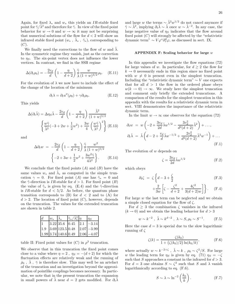
26

Again, for fixed λ∗ and w∗ this yields an IR-stable fixedpoint for γ/λ2 and therefore for γ. In view of the fixed pointbehavior for w → 0 and w → ∞ it may not be surprisingthat numerical solutions of the flow for d < 2 will show aninfrared stable fixed point (w∗ , λ∗ , γ∗), corresponding to(C).

We finally need the corrections to the flow of w and λ.In the symmetric regime they vanish, just as the correctionto ηS . The six-point vertex does not influence the lowervertices. In contrast, we find in the SSB regime

∆(∂tρ0) = −2vd

d

(1 − η

d + 2

)γ

λ

w

(1 + w)3/2ρ0. (E.11)

For the evolution of λ we now have to include the effect ofthe change of the location of the minimum

∂tλ = ∂tu′′(ρ0) + γ∂tρ0. (E.12)

This yields

∆(∂tλ) = ∆ηSλ − 2vd

d

(1 − η

d + 2

)λ2

(1 + w)5/2

wγ

λ2(−3 + 2w +

1

2w2) +

3w

4

(wγ

λ2

)2

(E.13)

and

∆∂tw = −2vd

d

(1 − η

d + 2

)γ

λ

w2

(1 + w)5/2

−2 + 3w +

1

2w2 +

3w2γ

4λ2

. (E.14)

We conclude that the fixed points (A) and (B) have the

same values w∗ and λ∗ as computed in the simple trun-cation γ = 0. For fixed point (A) one has γ∗ = 0 andthe γ-direction is IR-stable for d > 1. For fixed point (B)the value of γ∗ is given by eq. (E.4) and the γ-directionis IR-stable for d < 5/2. As before, the quantum phasetransition corresponds to (B) for d < 2 and to (A) ford > 2. The location of fixed point (C), however, dependson the truncation. The values for the extended truncationare shown in table 2.

d w∗ λ∗ γ∗/λ2∗ η ηS

1 3.22 35.6 0.45 2.1 −3.14

1.9 3.69 123.5 0.48 2.07 −3.99

1.99 3.74 140.6 0.49 2.06 −4.07

table II: Fixed point values for (C) in ρ3 truncation.

We observe that in this truncation the fixed point comesclose to a value where η = 2 , ηS = −(d + 2) for which thefluctuation effects are relatively weak and the running ofρ0 , λ , γ is therefore slow. This may well be an artefactof the truncation and an investigation beyond the approxi-mation of pointlike couplings becomes necessary. In partic-ular, we note that in the present truncation the expansionin small powers of λ near d = 2 gets modified. For ∂tλ

and large w the terms ∼ λ2w1/2 do not cancel anymore ifγ ∼ λ2, implying ∂tλ ∼ λ once w ∼ λ−2. In any case, thelarge negative value of ηS indicates that the flow aroundfixed point (C) will strongly be affected by the “relativisticdynamic term” ∼ V ϕ∗∂2

τϕ, as discussed in sect. IX.

APPENDIX F: Scaling behavior for large w

In this appendix we investigate the flow equations (72)for large values of w. In particular, for d ≥ 2 the flow fork → 0 necessarily ends in this region since no fixed pointwith w 6= 0 is present even in the simplest truncation.Including the “relativistic dynamic term” ∼ V one expectsthat for all d > 1 the flow in the ordered phase obeysw(k → 0) → ∞. We study here the simplest truncationand comment only briefly the extended truncations. Acomparison of the results for the simplest truncation in thisappendix with the results for a relativistic dynamic term insect. VIII demonstrates the importance of the relativisticdynamic term.

In the limit w → ∞ one observes for the equation (72)

∂tw = w

(−2 +

3vd

2dλw1/2 − 3v2

d

d2(d + 2)λ2

)+ . . . ,

∂tλ = λ

(d − 2 +

vd

dλw−1/2 +

2v2d

d2(d + 2)λ2w−1

)+ . . .

(F.1)

The evolution of w depends on

ζ =3vd

2dλw1/2 (F.2)

which obeys

∂tζ = ζ

d − 3 +

ζ

2(F.3)

+2

3w

[ζ − ζ2

d + 2+

4ζ2

3(d + 2)w

]. (F.4)

For large w the last term can be neglected and we obtaina simple closed equation for the flow of ζ.

For d ≥ 3 the combination ζ vanishes in the infrared(k → 0) and we obtain the leading behavior for d > 3

w ∼ k−2 , λ ∼ kd−2 , λ ∼ S, ρ0 ∼ S−1. (F.5)

Here the case d = 3 is special due to the slow logarithmicrunning of ζ

ζ(k) =ζ(k0)

1 +(ζ(k0)/2

)ln(k0/k)

, (F.6)

where actually w ∼ k−2+ζ , λ ∼ k , ρ0 ∼ ζ2/S. For largew the leading term for ηS is given by eq. (71) ηS = −ζsuch that S approaches a constant in the infrared for d > 3.For d = 3 one obtains S ∼ ζ2 such that S and λ vanishlogarithmically according to eq. (F.6).

S ∼ λ ∼ ln−2

(k0

k

). (F.7)

27

Also η vanishes for w → ∞ and the infrared behavior of theflow simply stops, with fixed ρ0 and A. For d > 3 the flowis ultraviolet dominated such that ξ−2

R = 2λ(k = 0)ρ0(k =0) ∼ λ(Λ)ρ0(Λ) = σ, corresponding to a critical exponentν = 1/2. We recall, however, that ξR only appears in theexponential decay of G11 for r → ∞, while G22 shows apowerlike decay given for η = 0 by eq. (49). For larger the correlation function 〈φ∗(~r)φ(0)〉 = 1

2 (G11 + G22) is

dominated by the “Goldstone contribution” G22.The situation is different for d < 3. Now the flow of ζ

exhibits a partial infrared fixed point

ζ∗ = 2(3 − d). (F.8)

The flow of w obeys near this fixed point (d 6= 2)

∂tw = (4 − 2d)w (F.9)

and we find the asymptotic behavior

w ∼ k4−2d , λ ∼ kd−2 , λ ∼ S,

ρ0 ∼ S−1k2(3−d). (F.10)

For d > 2 the asymptotic value of w increases and theflow always ends in the regime where w → ∞. For d < 3the infrared behavior of S depends on k and we obtain forζ = ζ∗ , w → ∞

ηS = 2(d − 3) , S ∼ k2(3−d). (F.11)

According to eq. (53) we note the modified relative scalingof time and space in the extreme infrared,

z = 2(d − 2). (F.12)

The anomalous dimension η vanishes in this limit. Weconclude that ρ0 reaches a constant value, while λ and Svanish asymptotically

λ ∼ S ∼ k2(3−d) , ρ0→ const. , A → const. (F.13)

Eq. (F.11) suggests that ηS increases monotonically withd. We may define dr such that ηS > −1 for d > dr. Eq.(F.11) would imply dr = 2.5. For d < dr the relativistickinetic term ∼ V dominates and the asymptotic equationsfor large w discussed in this appendix loose their validity.As we argue in sects. VIII, IX the linear kinetic term∼ S becomes subdominant for the infrared behavior of theGoldstone boson physics whenever S vanishes, i.e. for ηS ≤0. We conclude from eq. (F.11) that this happens for alldimensions d ≤ 3.

Even for d < dr only the infrared behavior in the denseregime is modified whereas other features continue to bereasonably represented by the simplest truncation. As anexample we may consider the correlation length for theradial mode. For the definition of the correlation lengthwe include only fluctuations with momenta ~q 2 > k2

ph =

ξ−2R , resulting in ξ−2

R = 2λ(k1)ρ(k1) with w(k1) = 1. The

behavior for w ≫ 1 corresponds to momenta ~q 2 ≪ ξ−2R

and does not affect the scaling ξR ∼ σ−1/2.

The particular scaling properties for 2 < d < 3 mainlyaffect the extreme infrared behavior of the propagator G11.For ~q 2 → 0 we may replace 2λρ0 → 2λ(~q)ρ0 with

λ(~q) = λ(k1)

(~q 2

k21

)− ηS2

. (F.14)

We expect a similar qualitative behavior even in presenceof the relativistic dynamic term. The value of ηS may bemodified, however. We argue that the infrared physics ford ≤ 3 is actually described by the d + 1-dimensional O(2)model. This suggests ηS = d − 3 instead of 2(d − 3). Thisyields the leading part of the static propagator G11

lim~q 2→0

G11 =1

2λ(k1)ρ0

(~q 2

k21

)d−3

. (F.15)

Summarizing our simplest truncation for the orderedphase, we find that for d > 2 the flow drives w alwaystowards large values and the condensate ρ0 or ρ0 settles ata constant value. For d > 3 also the interaction strengthλ and the coefficient S reach constant values, whereas for2 < d < 3 both λ and S vanish asymptotically. For d < 2,in contrast, the flow drives w towards a fixed point valuew∗. Indeed, starting with very large w eq. (F.9) impliesfor d < 2 a decrease of w. This continues until corrections∼ w−1 begin to be important.

For the upper critical dimension d = 2 the situation isspecial. The coupling λ becomes now a marginal coupling.For small enough λ the running effectively stops and we cantake a small λ as a free parameter. Expanding in powersof λ yields

∂tw = w

−2 +

λ

32π

w√1 + w

(3 +

4

1 + w− 27

(1 + w)2

),

∂tλ = (w − 2)2(1 + w)−5/2 λ2

16π. (F.16)

One finds an infrared stable (approximate) fixed point forlarge w

w∗ ≈(

64π

3λ

)2

. (F.17)

As λ moves slowly towards zero, w∗ increases to infinity.Indeed, for this fixed point the evolution of λ follows

∂t

(λ

16π

)≈ 3

4

(λ

16π

)3

(F.18)

implying a very slow running once λ(k) ≪ 16π

λ(k) = λ(k0)

1 +

3

2

(λ(k0)

16π

)2

lnk0

k

−1/2

. (F.19)

28

Here k0 denotes the scale where w ≈ w∗ becomes valid.The effective anomalous dimension is very small

η =3

2

(λ

16π

)2

. (F.20)

On the other hand, the flow equation

∂tS = 2S , ηS = −2 (F.21)

implies

S = S0k2

k20

, (F.22)

corresponding to the limit d → 2 of eq. (F.11). Similar to(F.13) we find the asymptotic behavior

λ = λS ∼ k2. (F.23)

The order parameter is approximately constant

ρ0(k) =k2

2S

(64π)2

9λ3=

(64π)2k20

18S0λ3. (F.24)

More precisely, the tiny running of ρ0 for large w∗ and d = 2may be directly inferred from eq. (27) (up to corrections∼ w−1

∗ )

∂tρ0 =λρ0

3π(1 + w∗)−3/2

= − 9λ4ρ0

(64)3π4= − ρ0

ln2 k0

k

.

(F.25)

The evolution of ρ0(k) stops for k → 0

ρ0(k) = ρ0(k0) exp

1

ln Λk0

− 1

ln Λk

. (F.26)

The flow of the bare order parameter ρ0 = ρ0/A

∂t ln ρ0 = ∂t ln ρ0 + η (F.27)

is dominated by η. For very small k < kl,

lnk0

kl≫ 2

3

(λ(k0)

16π

)−2

, (F.28)

one has

η ≈ ln−1(k0/k). (F.29)

This implies that ρ0(k) vanishes logarithmically for k → 0

ρ0(k) = ρ0(kl)ln(k0/kl)

ln(k0/k). (F.30)

We conclude that for d = 2 no long range order exists ina strict sense in this truncation. In this respect the upper

critical dimension d = 2 is similar to d < 2. In fact, wemay take the limit d → 2 of eq. (81) and observe that with

limd→2

ηS = −d (F.31)

the behavior ρ0 ∼ kη becomes essentially logarithmic as ηapproaches zero for d → 2.

Let us compare these findings with the true evolution inpresence of the relativistic kinetic term ∼ V . Without Vthe critical dimension below which order disappears wouldbe dc = 2. This is shifted to dc = 1 in presence of V .The presence of V reduces the disordering power of theGoldstone fluctuations. For a relativistic kinetic term theeffective power counting is different - the Goldstone regimecorresponds now to the classical model in dimension d + 1.

We conclude this appendix by addressing the issue of thescale kF associated to the density. We expect that for k ≫kF the density plays no role. The regime where the flow isessentially independent of the density effects correspondsto w ≪ 1. For k ≪ kF one expects a transition to a newqualitative regime where the density matters. This may beroughly associated with the Goldstone regime for w ≫ 1.

The transition between the Goldstone regime for w ≫ 1and the linear regime for w ≪ 1 typically occurs for w nearone and we may define the scale kG where w = 1 by

k2G ≈ 2λ(kG)ρ0(kG). (F.32)

The detailed relation between kF and kG may depend onthe dimension, but we expect that they are of a similarmagnitude. For a demonstration, we discuss this issue evenin our simplest truncation. Within the truncation (72) wehave found for d ≥ 2 that ρ0(k → 0) ≡ ρ0 approachesa positive constant. Since ρ0 scales proportional to thedensity we can define a dimensionless quantity

L = 2λρd−2

d

0 (F.33)

such that

w =Lρ

2d

0

k2. (F.34)

Since L is evaluated for k = kG we expect L to be a con-stant that is neither extremely small nor large. This implies

kG =√

Lρ1/d0 ∼ kF .

For d < 2 the issue is more involved. Besides w thecrossover to a relativistic kinetic term plays a role. Withinthe truncation (72) one may wonder where the scale setby the density appears in a situation for which the cou-plings w and λ flow to their fixed point values irrespectiveof their microphysical values. If all couplings are irrelevantthe information about the density would be lost in Γk→0.Expressed in terms of renormalized fields the effective ac-tion should therefore contain at least one parameter thatis not determined by the fixed point. Such a parameteris given by S and the presence of a scale can therefore beencoded in S, despite the fact that S is dimensionless. In-deed, the nontrivial scaling with ηS 6= 0 implies the genericform

S = S0

(k

k0

)−ηS

(F.35)

29

and a momentum scale appears by dimensional transmu-tation in the form of k0. Since the size of S determines thescale where V will start to dominate, it is plausible thatk0 can be related to the final value of ρ0 and therefore ton for d > 1. For d ≤ 1 the condensate contribution to thedensity ρ0 vanishes and the properties of G(~q) for ~q 6= 0play a decisive role.

We have avoided these subtle points by choosing a fixeddefinition (62) for kF . The price to pay is that the transi-tion between the qualitatively different behavior for thedense and the dilute regime occurs not necessarily forkph ≈ kF , but may involve a nontrivial proportionalityconstant.

APPENDIX G: Symmetries and thermodynamic

relations

In this appendix we summarize symmetries and Wardidentities [1], [4], [6] on the level of an appropriate trun-cation of the effective action [17]. Let us consider, forreal time (Minkowski signature), the classical action SM

in presence of local sources

SM =

∫

x

χ∗[i∂t + σ + (~∇− i ~A)2

]χ

−V (χ∗χ) + j∗χ + jχ∗

. (G.1)

Here σ(x) and ~A(x) are real source fields, while j(x) iscomplex. For a homogeneous setting the physical values

will be σ(x) = µ, ~A(x) = 0, j(x) = 0. The action is invari-ant under time- and space-translations, rotations, parityreflections xk → −xk, Ak → −Ak, as well as time reflec-tion t → −t, ϕ → ϕ∗, j → j∗. It is real and exhibits alocal U(1)-gauge symmetry associated to conserved parti-cle number

χ(x) → eiϑ(x)χ(x), j(x) → eiϑ(x)j(x),

Aµ(x) → Aµ(x) + ∂µϑ(x), (G.2)

where Aµ = (σ, ~A), ∂µ = (∂t, ~∇). For ~A = 0 the actionremains invariant under Galilei transformations

χ(t, ~x) → eifχ(t, ~x − 2 ~Pt), j(t, ~x) → eif j(t, ~x − 2 ~Pt),

f = ~P~x − ~P 2t, σ(t, ~x) → σ(t, ~x − 2 ~Pt). (G.3)

In eq. (G.1) we have scaled our units such that effectively2MB = 1, with MB the mass of the particles, such that

the velocity obeys ~v = ~P/MB=2 ~P . Thus for a plane wavewith ω = ~p2 the Galilei transformation indeed producesthe appropriate shifts in momentum and energy, ~p′ = ~p +~P , ω′ = (~p + ~P )2, i.e.

χ = ei(~p~x−ωt) → ei(~p′~x−ω′t). (G.4)

We note that Galilei transformations and ~x-dependent lo-cal U(1) transformations are not compatible. In the follow-

ing we take ~A = 0 and restrict the U(1)-transformations

to transformation parameters ϑ(t) depending on time butnot on the space coordinates.

Including the fluctuation effects yields the effective ac-tion Γ[ϕ, σ], with ϕ(x) = 〈χ(x)〉 evaluated for a corre-sponding source j(x). In absence of anomalies from thefunctional measure, and for T = 0, the effective action hasthe same symmetries as the classical action, where ϕ trans-forms in the same way as χ. This extends to the averageaction Γk if the cutoff Rk is consistent with the symme-tries. For an investigation of the long distance behaviorwe expand the effective action in the derivatives ∂t and ∆.Consistency with the symmetries requires

Γ =

∫

x

[U0(ρ) − 1

2Z(ρ)

ϕ∗[i∂t + σ + ∆

]ϕ + c.c

−1

2V (ρ)

ϕ∗[i∂t + σ + ∆

]2ϕ + c.c

+1

4Yt(ρ)ρ

∂2

t ρ − 2i∂t~∇(ϕ∗∇ϕ − ϕ~∇ϕ∗)

+2~∇(~∇ϕ∗∆ϕ + ~∇ϕ∆ϕ∗) − ∆(ϕ∗∆ϕ + ϕ∆ϕ∗)

−1

4Y (ρ)ρ∆ρ + ∆L

]. (G.5)

Here we use ρ = ϕ∗ϕ and ∆L contains further gradient

terms like (~∇ρ~∇ρ)2 or ~∇ρ~∇(ϕ∗(i∂t + σ + ∆)ϕ). In par-ticular, Galilei symmetry implies that all time derivativesappear only in the combination Dt = ∂t − iσ− i∆, and ad-ditional gradients act only on the invariants ρ and ϕ∗Dn

t ϕ.We next perform an analytic continuation to the eu-

clidean effective action by replacing −i∂t → ∂τ in eq.(G.5). (We have introduced an overall minus sign in thetransition from SM to Γ, such that the standard conven-tions for the classical action in Minkowski spacetime matchwith the standard conventions for the euclidean effectiveaction.) This allows for an extension to thermal equilib-rium with T 6= 0. For T 6= 0 additional terms can appearin the effective action. First, Galilei invariance is brokensince the heat bath singles out a particular reference frame.This permits the appearance of additional terms involvinggradients, as ϕ∗∆ϕ. Second, a continuation of the localU(1) invariance with real functions ϑ(τ) requires complexσ, transforming as σ → σ+ i∂τϑ. However, the real part ofσ is invariant under local transformations. In consequence,an arbitrary dependence of U, Z, V on σ+σ∗ becomes possi-ble. In practice, only the global U(1) symmetry is relevantfor T 6= 0, since the local transformations only constrainpossible couplings of the imaginary part of σ which playno physical role. The Ward identities related to the localU(1) symmetry and the Galilei transformations thereforeonly restrict the limiting behavior of Γ for T → 0. Weemphasize that all Ward identities are automatically im-plemented by the invariant form of Γ in eq. (G.5).

The effective potential in presence of a nonzero chemicalpotential σ reads

U(ρ, σ) = U0(ρ) − Z(ρ)ρσ − V (ρ)ρσ2. (G.6)

The order parameter is given by the condensate densitync = ρ0, which corresponds to the minimum of U at a

30

fixed value of σ

∂U

∂ρ |σ,ρ0

= 0 , ∂ρU0|ρ0= σ∂ρ(Zρ + σV ρ)|ρ0

. (G.7)

The total particle density is related to the σ-derivative ofU at ρ0

n = −∂U

∂σ(ρ0) =

[Z(ρ0) + 2σV (ρ0)

]ρ0. (G.8)

In terms of renormalized fields

φ = A1/2φ, ρ = Aρ, A = Z(ρ0) + 2σV (ρ0) (G.9)

one finds

n = ρ0. (G.10)

Thus a nonvanishing density requires for T = 0 a nonvan-ishing renormalized order parameter. (We recall that thereare ρ-independent contributions to U for T 6= 0. For exam-ple, a piece ∆U = −nT σ contributes to n a piece nT thatdoes not vanish for ρ0 = 0.) This observation is partic-ularly interesting for d = 1 where the consendate densityρ0 vanishes in the infinite volume limit. Indeed, we find adiverging A as the IR-cutoff k runs to zero.

We may also compute thermodynamic susceptibilitieslike the response of n to a change in the chemical potential

∂n

∂σ |T=0=

∂ρ0

∂σ= 2V (ρ0)ρ0 + S

∂ρ0

∂σ,

S = A

(1 +

∂ ln(Z(ρ0) + 2σV (ρ0)

)

∂ ln ρ0

). (G.11)

Differentiating the minimum condition (G.7) yields

∂ρ0

∂σ=

1

λ

∂n(ρ0, σ)

∂ρ0 |σ, λ =

∂2U(ρ, σ)

∂ρ2|σ,ρ0

, (G.12)

where

∂n

∂ρ0 |σ=

∂(Z(ρ0)ρ0

)

∂ρ0+ 2σ

∂(V (ρ0)ρ0

)

∂ρ0= S, (G.13)

and therefore

∂ρ0

∂σ=

S

λ,

∂n

∂σ |T=0=

2V (ρ0)n

A+

S2

λ. (G.14)

The pressure

p = −U(ρ0) (G.15)

is normalized such that it vanishes for T = n = 0, i.e.U0(ρ = 0) = 0. Its response to a change of the chemicalpotential obeys

∂p

∂σ |T= −∂U

∂σ |ρ0

− ∂U

∂ρ0 |σ,ρ0

∂ρ0

∂σ= n. (G.16)

In our units (2MB = 1) the energy density obeys ǫ = n/2and one obtains for the macroscopic sound velocity

c2s =

∂p

∂ǫ |T= 2

∂p

∂σ |T

(∂n

∂σ |T

)−1

. (G.17)

For T = 0 one finds

c−2s =

V (ρ0)

A+

S

2ρ0

∂ρ0

∂σ=

V (ρ0)

A+

S2

2ρ0λ. (G.18)

In presence of spontaneous symmetry breaking we areinterested in the propagator for small fluctuations aroundthe expectation value ϕ0 that we take here to be real. Wedecompose ϕ(x) = ϕ0 + 1√

2

(δϕ1(x) + iϕ2(x)

). The in-

verse propagator matrix is encoded in the part of Γ that isquadratic in δϕ1 and ϕ2. Retaining terms with up to twoderivatives one may parameterize

Γ2 =

∫

x

iS

2(δϕ1∂τϕ2 − ϕ2∂τ δϕ1)

−V

2(ϕ2∂

2τϕ2 + Brδϕ1∂

2τδϕ1) (G.19)

−1

2(ϕ2∆ϕ2 + Crδϕ1∆δϕ1) +

m2r

2δϕ2

1

.

Here we have defined the renormalized field ϕ such thatthe term ∼ ϕ2∆ϕ2 has coefficient one. For T = 0 wemay extract the different couplings by expanding eq. (G.5)(with λ = ∂2

ρU|ρ0)

Γ2 =

∫

x

i

2

[Z(ρ0) + 2σV (ρ0) + ρ0(∂ρZ + 2σ∂ρV )|ρ0

]

(δϕ1∂τ ϕ2 − ϕ2∂τ δϕ1)

−1

2V (ρ0)ϕ2∂

2τ ϕ2

−1

2

[V (ρ0) + ρ0(2 + ∂ρV + Yt + ρ∂ρYt)|ρ0

]δϕ1∂

2τ δϕ1

−1

2

[Z(ρ0) + 2σV (ρ0

]ϕ2∆ϕ2

−1

2

[Z(ρ0) + 2σV (ρ0)

+ρ0(2∂ρZ + 4σ∂ρV + Y + ρ∂ρY )|ρ0

](δϕ1∆δϕ1)

+λρ0δϕ21

. (G.20)

The renormalized field is the same as in eq. (G.9) and weidentify

S = 1 +∂ ln

(Z(ρ0) + 2σV (ρ0)

)

∂ ln ρ0=

S

A,

V =V (ρ0)

A,

Br = 1 + 2∂ ln V (ρ0)

∂ ln ρ0+

Yt(ρ0)ρ0

(V (ρ0)

(1 +

∂ ln Yt(ρ0)

∂ ln ρ0

),

Cr = 2S − 1 +Y (ρ0)ρ0

A

(1 +

∂ ln Y (ρ)

∂ ln ρ0

),

m2r = 2λρ0/A = 2λρ0 , λ =

λ

A2. (G.21)

31

We will find that S vanishes in the infinite volume limitfor d ≤ 3. The solution of eq. (G.21) implies that A(ρ)diverges for ρ → 0

A(ρ) = Z(ρ) + 2σV (ρ) → ρ0

ρ. (G.22)

For d > 1 one finds a nonzero ρ0 such that A = A(ρ0)remains finite. For d = 1, however, ρ0 → 0 and A divergesin the infinite volume limit. Since V remains finite also Vmust diverge ∼ ρ−1 in this case.

Comparing the definitions (G.11) and (G.21) one has

c−2s = V +

S2

2λρ0. (G.23)

For S → 0 this implies for the macroscopic sound velocity

c2s = V −1. (G.24)

In summary, Galilei and gauge symmetry relate forT = 0 the properties of the inverse propagator, like the mi-croscopic sound velocity v, the superfluid density nS = Aρ0

(as defined by the stiffness with respect to phase changes),

or the term linear in the frequency ∼ S, to macroscopicthermodynamic quantities. Using

∂n/∂σ = 2V n + S2/λ = 2n/c2s (G.25)

we can replace the σ-derivatives by n-derivatives or deriva-tives with respect to the volume Ωd (∂ lnn/∂ ln Ωd = −1for fixed particle number N)

∂ lnnc

∂σ=

2

c2s

∂ lnnc

∂ lnn= − 2

c2s

∂ lnnc

∂ ln Ωd. (G.26)

This gives a direct physical interpretation of the runningrenormalized couplings evaluated for k = 0

ρ0 = n = ns , ρ0 = nc , A−1 =nc

n= Ωc,

S

λ=

2n

c2s

∂ lnnc

∂ lnn,

V =1

c2s

(1 − S

∂ lnnc

∂ lnn

), cs = v. (G.27)

[1] N. Bogoliubov, J. Phys. (Moscow)11, 23 (1947);S. Beliaev, Sov. Phys. JETP 34, 289 (1958);N.Hugenholtz, D. Pines, Phys. Rev. 116, 489 (1959)

[2] S. Sachdev, Quantum Phase Transitions, Cambridge Uni-versity Press, Cambridge (1999);R. B. Laughlin, Adv. in Phys. 47, 943 (1998);D.V. Shopova, D. I. Uzunov, Phys. Rep. C379, 1 (2003);M. Vojta, cond-mat/0309604

[3] S. T. Beliaev, Sov. Phys. JETP 7, 289 (1958); 7, 299 (1958);J. Gavoret, P. Nozieres, Ann. Phys. (N. Y.) 28, 349 (1964);A. A. Nepomnyashchii, Y. A. Nepomnyashchii, JETP Lett.21, 1 (1975)

[4] P. B. Weichman, Phys. Rev. B38, 8739 (1988)[5] C. Castellani, C. Di Castro, F. Pistolesi, G. Strinati,

Phys. Rev. Lett. 78, 1612 (1997); F. Pistolesi, C. Castel-lani, C. Di Castro, G. Strinati, Phys. Rev. B69, 024513(2004)

[6] J. M. Kosterlitz, D. J. Thouless, J. Phys. C6, 1181 (1973)[7] K. G. Wilson, Phys. Rev. B4, 3174 (1971); K. G. Wil-

son, I. G. Kogut, Phys. Rep. 12, 75 (1974); F. Wegner, A.Houghton, Phys. Rev. A8, 401 (1973); J. Polchinski, Nucl.Phys. B231, 269 (1984)

[8] C. Wetterich, Nucl. Phys. B352, 529 (1991); Z. Phys. C48,693 (1990)

[9] C. Wetterich, Phys. Lett. B301, 90 (1993); Z. Phys. C57,451 (1993)

[10] J. Berges, N. Tetradis, C. Wetterich, Phys. Rept. 363, 223(2000)

[11] C. Wetterich, Int. J. Mod. Phys. A16, 1951 (2001)[12] J. Zinn-Justin, Quantum Field Theory and Critical Phe-

nomena (Oxford University Press 1989)[13] T. Gollisch, C. Wetterich, Phys. Rev. Lett. 86, 1 (2001)[14] M. Graeter, C. Wetterich, Phys. Rev. Lett. 75, 378 (1995);

G. v. Gersdorff, C. Wetterich, Phys. Rev. B64, 054513(2001)

[15] S. Tomonaga, Prog. Theor. Phys. 5, 544 (1950);J. M. Luttinger, J. Math. Phys. 4, 1154 (1963)

[16] S. Diehl, C. Wetterich, Phys. Rev. A73, 033615 (2006);Nucl. Phys. B770 [FS] 206 (2007)

[17] S. Floerchinger, C. Wetterich, to be published[18] D. Litim, Phys. Lett. B486, 92 (2000)[19] J. Adams, J. Berges, S. Bornholdt, F. Freire, N. Tetradis,

C. Wetterich, Mod. Phys. Lett. A10, 2367 (1995)[20] N. Tetradis, C. Wetterich, Nucl. Phys. B422 [FS], 451

(1994); L. Canet, B. Delamotte, D. Mouhanna, J. Vidal,Phys. Rev. B68, 064421 (2003); Phys. Rev. D67, 065004(2003); C. Bervillier, A. Juttner, D. Litim, hep-th/0701172

[21] D. I. Uzunov, Phys. Lett. A87, 11 (1981)[22] J. Berges, N. Tetradis, C. Wetterich, Phys. Rev. Lett. 77,

873 (1996)[23] T. Baier, E. Bick, C. Wetterich, Phys. Lett. B605, 144

(2005)[24] H. C. Krahl, C. Wetterich, Phys. Lett. A367, 263 (2007)[25] M. C. Birse, B. Krippa, N. R. Walet, J. A. McGovern,

Phys. Lett. B605, 287 (2005);S. Diehl, H. Gies, J. Pawlowski, C. Wetterich,cond-mat/0701198; cond-mat/0703366

[26] N. Dupuis, K. Sengupta, arXiv: 0709.0362 [cond-mat]