Quantum carpets of a slightly relativistic particle

www.fp-journal.org

Fortschritteder Physik

Progressof Physics

REPRINT

Quantum carpets of a slightly relativistic particle

Irene Marzoli1,, Alexander E. Kaplan2, Farhan Saif3, and Wolfgang P. Schleich4

1 Dipartimento di Fisica, Università di Camerino, 62032 Camerino, Italy2 Department of Electr. and Comp. Engineering, The Johns Hopkins University, Baltimore, MD 21218, USA3 Department of Electronics, Quaid-i-Azam University, Islamabad, Pakistan4 Institut für Quantenphysik, Universität Ulm, 89069 Ulm, Germany

Received 13 March 2008, accepted 13 March 2008Published online 23 May 2008

Key words Wave packets, one-dimensional box, Talbot effect, Green function.PACS 03.65.-w, 03.75.-b, 03.30.+p

We analyze the structures emerging in the spacetime representation of the probability density woven by aslightly relativistic particle caught in a one-dimensional box. In particular, we evaluate the relativistic effectson the revival time and the specific changes produced in the intermode traces, which quantum carpets consistof. Moreover, we present a detailed mathematical analysis of such quantum carpets pursuing the approach ofa kernel. Here we represent the probability distribution as a superposition of interfering Airy function-typestructures along straight world lines. We also show that this phenomenon can be enhanced by many orders ofmagnitude in semiconductors with narrow band-gap (e.g. as in InSb) and small effective mass of the electron,whereby due to the strong nonparabolicity of the semiconductor conduction band, the electron energy vsmomentum dispersion relation behaves in a pseudo-relativistic way.

Fortschr. Phys. 56, No. 10, 967 – 992 (2008) / DOI 10.1002/prop.200810535

Fortschr. Phys. 56, No. 10, 967 – 992 (2008) / DOI 10.1002/prop.200810535

Quantum carpets of a slightly relativistic particle

Irene Marzoli1,∗, Alexander E. Kaplan2, Farhan Saif3, and Wolfgang P. Schleich4

1 Dipartimento di Fisica, Universita di Camerino, 62032 Camerino, Italy2 Department of Electr. and Comp. Engineering, The Johns Hopkins University, Baltimore, MD 21218,

USA3 Department of Electronics, Quaid-i-Azam University, Islamabad, Pakistan4 Institut fur Quantenphysik, Universitat Ulm, 89069 Ulm, Germany

Received 13 March 2008, accepted 13 March 2008Published online 23 May 2008

Key words Wave packets, one-dimensional box, Talbot effect, Green function.

PACS 03.65.-w, 03.75.-b, 03.30.+p

We analyze the structures emerging in the spacetime representation of the probability density woven by aslightly relativistic particle caught in a one-dimensional box. In particular, we evaluate the relativistic effectson the revival time and the specific changes produced in the intermode traces, which quantum carpets consistof. Moreover, we present a detailed mathematical analysis of such quantum carpets pursuing the approachof a kernel. Here we represent the probability distribution as a superposition of interfering Airy function-type structures along straight world lines. We also show that this phenomenon can be enhanced by manyorders of magnitude in semiconductors with narrow band-gap (e.g. as in InSb) and small effective mass ofthe electron, whereby due to the strong nonparabolicity of the semiconductor conduction band, the electronenergy vs momentum dispersion relation behaves in a pseudo-relativistic way.

c© 2008 WILEY-VCH Verlag GmbH & Co. KGaA, Weinheim

1 Introduction

In this article we study the structures shown in Figs. 1 and 2, emerging in the spacetime representation of theprobability density of a slightly relativistic particle caught in a one-dimensional box. The first observationof these traces in a nonrelativistic box was in a computer simulation in [1]; however, no explanation of thecanals and ridges was suggested at that point. Motivated by this unusual feature in the probability densityof this most elementary quantum system we have studied these quantum carpets [2] in great detail [3–5].What we call here a “quantum carpet” is a rich and highly regular pattern in the quantum mechanical

probability density, |ψ(x, t)|2, describing the spatio-temporal evolution of wave packets [6]. So far, fourexplanations of non-relativistic quantum carpets have been put forward: (i) interference terms in the Wignerfunction [3], (ii) degeneracy of intermode traces [4], (iii) cancelation between appropriate terms in theenergy representation [7], and (iv) the kernel based on Green function [5].

In the present paper we generalize the approaches of intermode traces and Green function to the slightlyrelativistic particle. This problem is identical to the post-paraxial theory of Talbot images. Reference [8]has studied the post-paraxial propagator of the electric field or the wave function. The relevant sum involvesthe summation index in a quadratic or a quartic way. In contrast we study a kernel which is a quadraticform of the propagator. Consequently, the forth powers reduce to third powers which can be expressed interms of an Airy function.

∗ Corresponding author E-mail: [email protected], Phone: +39 0737 402534, Fax: +39 0737 402853

c© 2008 WILEY-VCH Verlag GmbH & Co. KGaA, Weinheim

968 I. Marzoli et al.: Quantum carpets of a slightly relativistic particle

7 9 11 13 150

0.4

3 5 7 9 110

0.4

11 13 15 17 190

0.4

T/2

(c)

00 L

(a) (b)

Fig. 1 (online colour at: www.fp-journal.org) Quantum carpets of a slightly relativistic particle caught in a box formedby the density plot of the probability density to find the particle at time t at position x. The initial wave functioncorresponding to three cases (a), (b), and (c) is a wave packet formed by the ground state wave function with the initialmomentum p = 7�k1 (a), p = 11�k1 (b), and p = 15�k1 (c). The grey scale ranges from white (low probability)to black (high probability). The dashed line marks the revival time T/2 of the non-relativistic particle. The upperdiagrams show the populations of the different energy levels of the box, labeled by the quantum numbers. For allcarpets we have chosen the relativistic parameter q = 10−2.

The design of a quantum carpet reflects a large-scale interference between many excited eigenmodesof the system. The key mechanisms for this pattern formation are [4] the pair interference between eigen-modes of the system, each term resulting in what we call an “intermode trace”, and the degeneracy of thesetraces. We have also demonstrated [4] that these traces exist in any anharmonic potential, although theyare most pronounced in the case of the non-relativistic box potential, since the box has the highest possibledegeneracy. This property comes from the perfectly quadratic spectrum, a characteristic common to otherrotorlike systems.

1.1 Quantum carpets in various quantum systems

Quantum carpets have become rather popular. They manifest themselves in many quantum systems wherethe energy spectrum displays an almost quadratic dependence [9]. They originate from the Talbot effect of

c© 2008 WILEY-VCH Verlag GmbH & Co. KGaA, Weinheim www.fp-journal.org

Fortschr. Phys. 56, No. 10 (2008) 969

0 5 10 15 20 25 30

0.02

0.04

0.06

0.08

0 5 10 15 20 25 30

0.025

0.05

0.075

0.1

0.125

0.15

0.175

0 L0

(a) (b)

T/2

Fig. 2 (online colour at: www.fp-journal.org) Quantum carpets of a slightly relativistic particle caught in a box whenthe initial wave function is a Gaussian wave packet located at the center of the box with a width Δx = L/20 and anaverage momentum p = 5�k1 (a) or p = 10�k1 (b). The grey scale, the marking of the non-relativistic revival timeT/2, and the population diagrams are indicated as in Fig. 1.

classical optics [10] but have also been observed experimentally in atom optics [11]. More recently theyappeared in wireless transfer between antenna arrays at the Talbot distance [12]. Moreover, wave packetsof Rydberg electrons display quantum carpets as shown in [13].

Quantum carpets are not limited to systems where the time evolution is governed by the linear Schro-dinger equation. Even a Bose-Einstein condensate (BEC) can weave [14] a quantum carpet. However, they

www.fp-journal.org c© 2008 WILEY-VCH Verlag GmbH & Co. KGaA, Weinheim


are not restricted to bosons but also appear for fermions [15]. In the case of cold atoms the confining wallsare made out of light sheets as realized experimentally in [16].

Moreover, quantum carpets can display fractal features. They manifest themselves either in the timeevolution [17] or as fractal noise in quantum ballistic and diffusive lattice systems [18]. Even a Bohmianapproach [19] towards quantum fractals based on quantum carpets has been suggested.

Quantum walks [20] have been in the center of interest in the context of quantum information. They pro-vide an enhanced diffusion compared to Brownian motion and are therefore useful for search algorithms.In this context quantum carpets have also been found [21] in continuous-time quantum walks.

We conclude by mentioning that an analysis of quantum carpets based on number and group theoreticaltools suggests possible application to integer factorization [22] by means of base-N quantum computingregisters [23].

1.2 Why relativistic corrections?

We have briefly addressed the relativistic modifications [4] of the trace trajectories as perhaps the most fun-damental yet very small factor to break the degeneracy and found relativistic corrections to the intermodetrace velocities. In particular, we have shown that the maximum relative correction is of the order

|Δ| ∼ Emax

mec2∼ β2

2, (1)

where Emax is the maximum excitation energy of the electron in the system and β ≡ vmax/c. For anexcitation energy Emax ∼ 0.5 eV we find with me = 9.1095 × 10−31 kg and c = 2.9979 × 108 m/s themaximum relative correction |Δ| ∼ 10−6.

In this paper we make a detailed exploration of the slightly relativistic corrections and observe a fewremarkable features: (i) The velocity dependence of the mass amends the “velocities” of the intermodetraces, which was natural to expect; (ii) In spite of the relativistic nonlinearity, the entire pattern still showsa strong revival (at least in the first few revival cycles), which is a less expected effect. This phenomenonis mostly due to the fact that the group of excited levels, engaged in the motion, is relatively tight and toa great extent the degeneracy is almost intact, while the entire spectrum is relativistically expanded. Weestimate the shift of the revival time, which increases with the excitation energy.

One might argue that under regular laboratory conditions, with the electron energy being of just afew eV, such small slightly relativistic corrections would be insignificant and negligible. Nevertheless,even these extremely tiny modifications of the classical trajectory can produce large nonlinear effects on asufficiently long time scale. The case of reference is the hysteretic cyclotron resonance [24, 25] of a singleelectron in a magnetic field, predicted in [24] and experimentally observed in [26]. Indeed, the excitationenergy of the electron in the experiment [26] was typically smaller than 1 eV and theoretical estimates [24]showed that it could even go lower, down to 10−3 eV.

The slight relativistic mass effect of the free electron in vacuum is the basis of the cyclotron maser, that isthe gyrotron [27]. Furthermore, since conduction electrons in narrow-gap semiconductors exhibit a pseudo-relativistic behavior [28], it was proposed to develop a solid-state cyclotron maser [29] by exploiting thepseudo-relativistic behavior of conduction electrons in semiconductors. Indeed, the dispersion relationbetween the conduction-band energy and the momentum closely resembles the expression for the energyof a relativistic particle, in which the speed of light c is replaced by a characteristic velocity v0 determinedby the energy gap and the effective mass of the conduction electron. Therefore, our considerations on thequantum carpets of a slightly relativistic particle apply to these systems as well. The pseudo-relativisticvelocity domain is easily accessible and the nonlinear mass dependence on momentum has been shown toproduce also a hysteretic bistable cyclotron resonance [30]. The enhancement of the relativistic effects innarrow-gap semiconductors is estimated as the ratio of the rest-energy of a free electron to the band-gap,and could be as large as a few orders of magnitude in comparison to the free-electron case.


Fortschr. Phys. 56, No. 10 (2008) 971

1.3 Overview

Our paper is organized as follows. In Sec. 2, we briefly review the concept of intermode traces [4] in thespatio-temporal dynamics of a wave packet in a non-relativistic multi-level quantum system prepared bya broad-band excitation and weaving quantum carpets. We then generalize in Sec. 2.2 the theory of thesetraces to the problem of a slightly relativistic electron in a box with infinitely high walls. Section 3 isdedicated to a discussion of the quantum revival. In most of the cases of interest, it remains a strongly pro-nounced effect that can be used as a “global” indicator and a measurement parameter of the phenomenon.We illustrate these new results with the quantum carpets in the simplest cases, whereby the original wave-function is either a ground state, or a very narrow wave packet with the spatial width much shorter thanthat of the box.

So far we have used qualitative arguments to explain the canals and ridges in the case of the relativisticparticle and presented numerical estimates of the size of the effects. In the remaining sections we pursuea more mathematical approach. In Sec. 4 we introduce the concept of the kernel which allows us to castthe probability densityW into a double integral of the product of the initial wave function and its complexconjugate and the kernel. The latter consists of the product of the Green function and its complex conjugate.We then derive in Appendix A an explicit expression for the kernel in terms of an infinite sum of Airyfunctions and dedicate Sec. 5 to a discussion of this formula. In Sec. 6 and Appendices B and C, weevaluate the double integral for a Gaussian initial wave packet and discuss the emerging carpets. Theprobability distribution of a non-relativistic particle is recovered in Appendix D as a limiting case of themore general expression for a slightly relativistic particle.

In Section 7, we analyze the possibility of using the pseudo-relativistic behavior of conduction elec-trons in semiconductors, and show that the sensitivity of intermode traces to the relativistic excitation canbe enhanced by many orders of magnitude. This fact suggests a very realistic way for the experimentalobservation and a possible application of quantum carpets to the characterization of semiconductors. Weconclude by summarizing our main results in Sec. 8.

2 Intermode traces

In a way of a technical introduction to quantum carpets, that is highly-organized patterns of intermodetraces, we first review in this section the formation of non-relativistic intermode traces in a one-dimensional(1D) “quantum box” [4]. A 1D square well potential with infinite walls, that is a box, is probably the bestmodel to demonstrate intermode traces, since all its eigenfunctions and eigenenergies are well-known andelementary. We then address the corresponding problem of a slightly relativistic particle. Here we deriveapproximate but analytical expressions for the relevant eigenfunctions and energies.

2.1 Non-relativistic particle

2.1.1 Wave equation

We recall that the Schrodinger equation for the wave function ψ(x, t) of a non-relativistic particle withmass M , moving along the x-axis in a box of length L with 0 ≤ x ≤ L reads

i�∂ψ

∂t− Hψ = 0, (2)

where � is Planck’s constant and

H ≡ − �2

2Md2

dx2(3)

is the non-relativistic Hamiltonian consisting only of kinetic energy.



It is worth noting that Maxwell equations of classical electrodynamics can also be approximated bythe same equation under the assumption of small diffraction and fixed polarization, that is in the so-calledparaxial approximation. In the resulting scalar equation, the wave function ψ is replaced by the field am-plitude E , the operator d2/dx2 by the “transverse” Laplacian, the time t by the longitudinal coordinate zof propagation, and � by the wavelength λ. The limits � → 0 and λ → 0 correspond to classical mechan-ics and ray optics, respectively. Thus, the basic theory of intermode traces involves either spatio-temporalpatterns in quantum mechanics with one coordinate and a time variable, or spatial patterns in optics withone transverse and one longitudinal variable. In the electromagnetic analogy, the wavefunction in a squarebox with infinite walls corresponds to an electromagnetic wave in a waveguide with ideal metallic walls.

2.1.2 Elementary intermode terms

The time evolution of a particle is described by the superposition

ψ(x, t) =∞∑

m=1

ψmum(x)e−iEmt/�, (4)

of energy eigenfunctionsum(x) with energiesEm and amplitudesψm determined by the initial conditions.For a box of width L these wave functions read

um(x) ≡{ √

2/L sin(kmx), for 0 ≤ x ≤ L,

0, otherwise.(5)

The eigenfrequencies, energies, and wave numbers

ωm ≡ m2ω1, Em ≡ �ωm, and km ≡ mk1 (6)

are in terms of the ground state frequency, energy, and wave number

ω1 ≡ �π2

2ML2, E1 ≡ �ω1, and k1 ≡ π

L. (7)

To bring out the spatio-temporal patterns of the probability density, |ψ|2, we represent it as a sum

|ψ(x, t)|2 ≡∞∑

m,n=1

μmn(x, t), (8)

of elementary intermode terms

μmn(x, t) ≡ ψ∗mψnum(x)un(x)ei(Em−En)t/�. (9)

We now break up the density Eq. (8) into the time-independent term

I0(x) ≡∑

m

μmm(x) (10)

with all the diagonal components μmm ≡ |ψm|2u2m(x), where |ψm|2 are the populations of the corre-

sponding quantum levels, and the “interference” term,

Iint(x, t) ≡∑

m �=n

μmn(x, t) (11)

which is the sum over all the non-diagonal components. Its average over a long time vanishes but it helpsus to keep a global view of the spatio-temporal evolution of |ψ|2.


Fortschr. Phys. 56, No. 10 (2008) 973

Since each of the energy eigenfunctions Eq. (5) is a superposition of plane waves, exp(±ikmx −iEmt/�), the elementary interference term μmn for m �= n consists of plane waves exp(±iζmn), withthe phase

ζmn(x, t) ≡ (km ± kn)x ± (Em − En)t/� + (Cmn)0, (12)

where (Cmn)0 are constants.Note that the two pairs of signs, ±, in front of both momentum and energy, are independent of each

other, so that in Eq. (12) we have four different phases ζmn(x, t).

2.1.3 Velocity of intermode traces

The lines of constant phase, ζmn(x, t) ≡ const, form spacetime trajectories which define the intermodetraces with their “velocities” [4]

vmn ≡(dx

dt

)

mn

= ± (Em − En)/�km ± kn

, (13)

or

vmn = ±S · vbox, S = m± n; (14)

where S is a normalized velocity and

vbox ≡ �k1

2M=cλc

4L� c, (15)

is a characteristic velocity, and λc ≡ h/(Mc) is the Compton wavelength.Since S in Eq. (14) is an integer, a trace with a certain S is attributed to all the couples of modes m

and n whose sum or difference is S. If the number of the states involved is sufficiently large, this tracedegeneracy creates multiple superimposed traces. They in turn give rise to the distinct straight canals in thetrace trajectory:

xmn = vmnt+ (xmn)0 = ±S · vboxt+ (xmn)0, (16)

where (xmn)0 is a constant.The lowest possible trace velocity, (vmn)min = vbox, or |S| = 1, corresponds to |m − n| = 1 and is

equal to the phase velocity, ω1/k1, of the ground state. In general, the traces that correspond to the “+” signin the term km ± kn in Eq. (13) and low S, have very low velocity and describe strictly quantum featuresof the motion. In contrast, if the excitation of the system is sufficiently high, i.e. the most populated energylevels are concentrated near some high quantum number m � 1, the “−” sign in the term km ± kn inEq. (13) creates the terms with high normalized velocity S ∼ 2 · m. In this case vmn is approachingthe group velocity, vgr, that corresponds to the classical motion of the particle. Indeed, an initially almostclassical motion is described by a compact group of eigenmodes near the quantum number m, with a spreadΔm of these modes satisfying the condition 1 � Δm � m. This excitation results in a strong clusteringof traces in two groups. The one with

|(Δω)mn| � ωm, and (Δk)mn � |km|, (17)

where (Δω)mn ≡ ωm − ωn, and (Δk)mn ≡ km − kn, is essentially a classical trajectory, since in such acase

(Δω)mn

(Δk)mn≈ dω

dk≡ vgr. (18)



It coincides with the classical velocity, since the intermode trace equation obtained from Eq. (14) as

dx

dt=

√2Em

M, (19)

describes the classical motion of a particle with energyEm.We conclude by noting that the other group of traces, with

vmn � vgr, and |km ± kn| ≈ |2km|, (20)

reflects the quantum behavior. The full set of velocities vmn defined by Eq. (14), ranging from groupvelocity to phase velocity at the extremes, provides a greatly useful new tool in the understanding of aquantum system.

2.2 Slightly relativistic particle

The degeneracy of some of the traces in the ideal box can be lifted either by a different form, such as theanharmonic potential [4], or by relativistic corrections. They provide the most fundamental perturbation,although in realistic settings they are very small [4]. However, in Sec. 7 we show that in semiconductorswith narrow bandgaps and a strong pseudo-relativistic dependence of energy on momentum, they maybecome sufficiently pronounced.

2.2.1 Wave equation

We start from the relativistic Hamiltonian

H ≡√

(Mc2)2 + (pc)2 −Mc2

= Mc2

[√1 +

( p

Mc

)2

− 1

](21)

of a particle of mass M and expand the square root into powers of p/(Mc) which yields

H p2

2M− 1

2Mc2

(p2

2M

)2

. (22)

The time independent Schrodinger equation for the slightly relativistic particle then reads[p2

2M− 1

2Mc2

(p2

2M

)2]um = Em um. (23)

Since the momentum operator

p ≡ �

i

∂

∂x(24)

corresponds to a differentiation Eq. (23) is a differential equation of fourth order. Here, we do not wantto go into subtle questions such as additional boundary conditions, but note that we have to maintain theboundary conditions

um(x = 0) = um(x = L) = 0 (25)

enforced by the walls at x = 0 and x = L. This feature suggests the ansatz

um(x) = sin(kmx) (26)


Fortschr. Phys. 56, No. 10 (2008) 975

with the wave number

km ≡ mπ

L. (27)

When we substitute this ansatz into the Schrodinger equation we arrive at{

(�km)2

2M− 1

2Mc2

[(�km)2

2M

]2− Em

}sin(kmx) = 0 (28)

which leads to the dispersion relation

Em =(�km)2

2M− 1

2Mc2

[(�km)2

2M

]2. (29)

The expression Eq. (27) for the wave number reduces this formula to

Em = (m2 − q2m4) �2πT

(30)

where we have introduced the ratio

q ≡(

2π�

Mc

)/4L ≡ λc

4L(31)

between the Compton wavelength λc of the particle and the length of the box.Moreover, we have expressed the energy in terms of the revival time

T ≡ 4ML2

π�(32)

of the non-relativistic particle in the box.We conclude by presenting the normalized energy eigenfunctions

um(x) =

√2L

sin(mπ

x

L

)(33)

of the slightly relativistic particle.

2.2.2 Velocity of intermode traces

The trace velocities Eq. (14) are then modified in such a way that the degeneracy is lifted(dx

dt

)

mn

= ±(n±m) · [1 − q2 · (n2 +m2)] · qc. (34)

Since the relativistic correction in Eq. (30) is presumed to be small, i.e. q2m2 � 1, and the number ofexcited levels is not too large, i.e. if |Em − E| � E, with E1 � E being a sufficiently large averageenergy of excitation, we can approximately write Eq. (30) in a more intuitive way

Em ≈ m2 ·E1

(1 − q2

E

E1

)= m2 · E1

(1 − E

2Mc2

). (35)

The average relative correction in Eq. (34) is then

Δ ≡ q2 · (n2 +m2) ≈ E/(Mc2). (36)

For the example of an electron, that is M = me we find for a 0.5 eV excitation an average relativecorrection Δ ∼ 10−6. However, we will show in Sec. 7 below that this correction can be enhanced byorders of magnitude in narrow band-gap semiconductors, where the conduction electrons, beside exhibitinga relativistic-like behavior, also have greatly reduced effective mass.



3 Quantum revival

How can we observe and measure the predicted relativistic changes in the maze of intermode traces? Ofcourse, we could isolate some individual traces and measure the change of their “velocities” vmn, Eq. (34).However, due to the finite spacing between the traces, the uncertainty of determining their velocities haveto be dealt with. Another approach, at least for proof-of-principle measurements, would be to look at theclearly visible changes in the global picture, such as the revival of the quantum packet, whose characteristictime can be measured with good precision.

But we would also expect that, because of the relativistically-induced removal of the trace velocitydegeneracy, Eq. (34), the revival would also be suppressed or spread. Surprisingly and fortunately, forall practical purposes this does not happen for most of the experimental conditions. Based on heuristicarguments we now derive the energy dependence of the revival time and then confirm these predictions bynumerical simulations presented in Figs. 1 and 2.

3.1 Energy dependence of revival time

Indeed, if we choose the initial state of the system to be simply its ground state as shown Fig. 1 and insuressufficient excitation of the system, that is 1 � n2,m2 in Eq. (34), the “spreading”, ΔT , of the revival timewill be much smaller than the relativistic change of that time, δT , the ratio of them being

ΔTδT

∼ Δmm

∼ O(1)m

∼ O(1)

√E1

E� 1. (37)

The major factor, that contributes to this “almost-conserved” revival, is the fact that if we start with theground state as the initial one, the total number of excited states remains always small and almost constant,regardless of how strong the excitation is , and whether it is relativistic or not. Indeed, the theory of δ-excitation [31] shows that if we want to account for say 95% of the total probability,

∑∞m=1 |ψm|2 = 1,

it is enough to include in this sum the most likely state with quantum number m ∼√E/E1, and no

more than a pair of adjacent states with their quantum numbers being m = m ± 1 and m = m ± 2. Thissimplification is confirmed by Fig. 1. Thus, writing the term (n2 +m2) as

n2 +m2 = (m+ Δn)2 + (m+ Δm)2, (38)

where

|Δn|, |Δm| = O(1) � m, (39)

we arrive at the formula,

n2 +m2 ≈ 2m2

[1 ± O(1)

m

], with 1/m� 1, (40)

which essentially amounts to Eq. (37). Hence, Eqs. (35) and (36) are valid with great precision.The revival time Trev is a purely quantum characteristic of the system; in our case, it is determined by

the smaller trace velocity, vq with |n−m| = 1 in Eq. (34), as

Trev

2=

L

|vq| ≈L/(qc)

1 − 2q2m2=T

2

(1 +

E

Mc2

), (41)

where T is the non-relativistic revival time defined in Eq. (32).The natural linear increase of Trev with the increased energy of excitation is consistent with our com-

puter simulations underlying Fig. 1. In fact, Eq. (41) suggests the interesting generalization

Trev = T · γ, (42)


Fortschr. Phys. 56, No. 10 (2008) 977

for a fully relativistic case of arbitrary kinetic energyE of excitation where

γ = 1 +E

Mc2(43)

is the relativistic factor. Needless to say, this conjecture requires a prove using a full scale relativisticapproach based on Dirac equation, which we plan to pursue in our future research.

3.2 Simulations

In Fig. 1 we show the traces predicted by Eq. (34). The initial wave packet here is the ground state wavefunction, u1(x) ∝ sin(πx/L). The system is hit by a δ-pulse delivering a momentum p, which we normal-ize to the ground state momentum p1 = �k1. The resulting spectrum of excitation encompasses always thesame small number of energy levels around the average state labeled by the quantum number m, shownin the top of Fig. 1. Moving from case (a) to (c) we increase the average excitation energy, in order tobetter fulfil the condition set in Eq. (37). Indeed, we confirm that the revival time increases linearly withthe average excitation energy, as predicted by Eq. (41) and that the quantum carpets are not washed out.Remarkably enough, even in case (c) the revival is still clearly present despite the relativistic correctionq2m2 to the eigenenergies is most pronounced. This is an apparently amazing result, but in light of Eq. (37)a strongly excited wave packet is more likely to revive at least once; furthermore, the traces become morepronounced and ordered, lending themselves for easier observation and measurements.

Interestingly enough, even when the initial state of the system is not a ground state, but a mixed statein which many quantum levels are engaged such as a Gaussian wave packet whose width is much smallerthan the size L of the quantum well the first revival can still be well identified, although the expected areaof revival is being spread somewhat as indicated in Fig. 2. The higher order revivals are getting spreadin a more drastic way. The amazing fact apparent from Fig. 2 is that when the energy of the excitation isincreased, the entire system of traces becomes much better organized and the individual traces, as well asthe first revival, are much more easily identified and “traceable”.

The key to this effect is the fact that for sufficiently low initial momentum delivered to the particle witha very narrow initial quantum packet (in both cases in Fig. 2, the ratio of that width to the well width, L, isabout 1/20), we have two different quantum kinetic processes going on simultaneously. One corresponds tothe almost classical bouncing of a particle between the walls due to the initial momentum p accompaniedby quantum spreading, while the other corresponds to the purely quantum spreading, symmetrical withrespect to the middle of the well, of the narrow wave package (engaging many quantum levels from thevery beginning). This feature stands out most clearly in the population diagram of the excited levels forcase (a), which consists of two sub-groups of excited levels: one of them having its maximum at theground state, with this sub-group corresponding to a pure quantum spreading, while the other one, withits maximum shifted away from the ground state, corresponds to the kinetic motion of the particle. In thatparticular case, the probabilities of the particle being engaged into one or another motion are of the sameorder of magnitude. In case (b), where the initial momentum delivered to the particle, is roughly double ofthat of case (a), and therefore the kinetic energy is expected to be four times of that of case (a), we see thatalmost all the excitation goes into kinetic (classical plus quantum) motion. The population diagram showsnow a tight group of levels, which is completely separated from the ground state. Considerations, similar tothose made for the case in which the system is initially in its ground state, indicate that the entire quantumcarpet is much more ordered and have very straight traces, than for the “mixed” dynamics of case (a).

4 Green function and kernel

So far we have used qualitative arguments to explain the canals and ridges in the spacetime representationof the probability density W (x, t) ≡ |ψ(x, t)|2 of finding a slightly relativistic particle at the position x attime t. We now study this density from a more mathematical point of view.



The most convenient way to obtain this density is to use the Green function. In the present section webriefly review the relevant ingredients.

The time dependent wave function ψ(x, t) of a particle moving in a one-dimensional potential reads

ψ(x, t) =∫ L

0

dx′G(x, t|x′)ϕ(x′). (44)

Here ϕ(x) ≡ ψ(x, t = 0) denotes the initial wave function and the Green function

G(x, t|x′) ≡∞∑

m=1

um(x)um(x′) e−iEmt/� (45)

consists of the energy eigenfunctions um(x) with energy Em.Hence, the probability density

W (x, t) ≡ |ψ(x, t)|2

=∫ L

0

dx′∫ L

0

dx′′K(x, t|x′, x′′)ϕ∗(x′)ϕ(x′′) (46)

follows from the integration of the kernel

K(x, t|x′, x′′) ≡ G∗(x, t|x′)G(x, t|x′′) (47)

and the wave functions ϕ(x′′) and ϕ∗(x′).

5 Discussion of the kernel

In Appendix A we use the energy eigenfunctions of a slightly relativistic particle derived in Sec. 2.2 toobtain the Green function, Eq. (45), and the kernel, Eq. (47), of this problem. The resulting kernel

K(x, t|x′, x′′) =1

4L2

∞∑

j,l=−∞(−1)jl |βj(t)|

×{

exp(iπj

x′ − x′′

2L

)Ai[βj(t)

(χj,l − x′ + x′′

2L

)]

+ exp(−iπj x

′ − x′′

2L

)Ai[βj(t)

(χj,l +

x′ + x′′

2L

)]

− exp(iπj

x′ + x′′

2L

)Ai[βj(t)

(χj,l − x′ − x′′

2L

)]

− exp(−iπj x

′ + x′′

2L

)Ai[βj(t)

(χj,l +

x′ − x′′

2L

)]}

(48)

contains the world lines

χj,l(x, t) ≡ x

L−(j − 1

2q2j3

)t

T/2− l (49)


Fortschr. Phys. 56, No. 10 (2008) 979

and

βj(t) ≡ sign(j)π(3πq2|j|t/T )1/3

. (50)

Here, T ≡ 4ML2/(π�) denotes the revival time of the non-relativistic particle in the box and Ai is theAiry function.

The expression Eq. (48) for the kernel together with Eqs. (49) and (50) is the key result of the presentpaper. We now discuss the main properties of K .

We first note that the kernel consists of a superposition of products of phase factors and appropriatelyscaled Airy functions. The arguments of the Airy functions contain the quantity χj,l, a scaled time variableβj(t) and the integration variables x′ and x′′. Here, an interesting factorization property comes to light.Whenever the phase factor contains the difference x′ − x′′ of the integration variables the argument ofthe Airy functions contains the sum x′ + x′′, and vice versa. This feature will become important whenwe perform the integrations over the coordinates and the initial wave packet enjoys the same factorizationproperties.

Moreover, the quantity χj,l describes straight lines in spacetime which cross the x axis at integers land whose steepness is governed by j − q2j3/2. This feature suggests that the spacetime structures inthe probability density should be also straight lines with the steepness slightly modified by the relativisticparameter q. However, Fig. 3 shows that this conjecture is not correct. The blurred spacetime structuresfollow curved world lines. This deviation from the intuition is due to the behavior of the Airy functionand the time dependence of the function βj(t) in its argument. For short times the Airy function showsa dominant maximum which is reminiscent of a localized Gaussian function. For larger times many sidemaxima emerge. This long range oscillatory tail leads to extended interference effects among several termsin the expression Eq. (48) of the kernel and results in a distortion of the original pattern of straight lines inthe probability density. The form of the initial wave packetϕ(x) determines how many of these oscillationssurvive. To bring this out more clearly we study in the next section a specific wave packet.

6 Gaussian wave packet

So far we have discussed the properties of the kernel. In the present section we analyze how they maponto the time evolution of a wave packet. Here we focus on an initial wave packet which satisfies the samefactorization condition as the kernel. For this reason, we concentrate on the case of a Gaussian initial wavepacket

ϕ(x) ≡ (√πΔx)−1/2 exp

[− 1

2

(x− x

Δx

)2]eip(x−x)/� (51)

of width Δx centered at x and moving with average momentum p ≡ j�π/(2L) > 0.When the width Δx is much smaller than the width of the box we can extend the integrations in Eq. (46)

determining the probability density to minus and plus infinity and evaluate the integrals in an exact way.According to Appendix B the probability density of a slightly relativistic particle reads

W (x, t) =√πΔx2L2

∞∑

j,l=−∞(−1)jl

×{

exp

[−(j − j

Δj

)2]Aj

(χj,l − x

L, t

)+ exp

[−(j + j

Δj

)2]Aj

(χj,l +

x

L, t

)

− 2 exp

[−(

j

Δj

)2]

exp

[−(

j

Δj

)2]

Re[eiπjx/LAj

(χj,l + i2πε2j, t

)]}. (52)



0

T/2

0

T/2

0 L

0 L

Fig. 3 Quantum carpets of a slightly relativistic particle in their dependence on the initial momentum and the relativis-tic parameter. Spacetime representation of the probability density W (x, t) for an initial Gaussian wave packet centeredat x = L/2 and width Δx = L/20. The grey scale ranges from white for the minima to black for the maxima. Theaverage momentum takes up the values p = 0 (left), p = 10�π/(2L) (center) and p = 20�π/(2L) (right). The upperdiagrams refer to cases with the relativistic parameter q2 = 10−4, while the lower ones correspond to q2 = 10−3.


Fortschr. Phys. 56, No. 10 (2008) 981

T/8

T/8

0

0

L0

L0

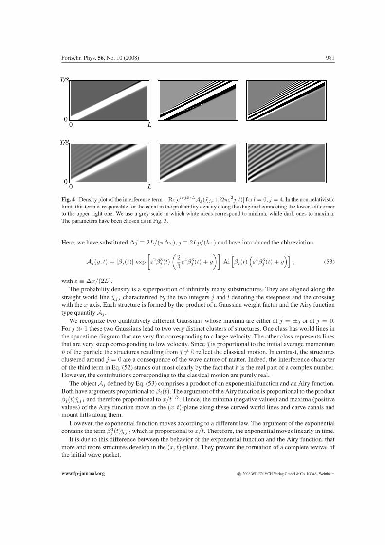
Fig. 4 Density plot of the interference term −Re[eiπjx/LAj(χj,l+i2πε2 j, t)] for l = 0, j = 4. In the non-relativisticlimit, this term is responsible for the canal in the probability density along the diagonal connecting the lower left cornerto the upper right one. We use a grey scale in which white areas correspond to minima, while dark ones to maxima.The parameters have been chosen as in Fig. 3.

Here, we have substituted Δj ≡ 2L/(πΔx), j ≡ 2Lp/(�π) and have introduced the abbreviation

Aj(y, t) ≡ |βj(t)| exp[ε2β3

j (t)(

23ε4β3

j (t) + y

)]Ai[βj(t)

(ε4β3

j (t) + y)]

, (53)

with ε ≡ Δx/(2L).The probability density is a superposition of infinitely many substructures. They are aligned along the

straight world line χj,l characterized by the two integers j and l denoting the steepness and the crossingwith the x axis. Each structure is formed by the product of a Gaussian weight factor and the Airy functiontype quantity Aj .

We recognize two qualitatively different Gaussians whose maxima are either at j = ±j or at j = 0.For j� 1 these two Gaussians lead to two very distinct clusters of structures. One class has world lines inthe spacetime diagram that are very flat corresponding to a large velocity. The other class represents linesthat are very steep corresponding to low velocity. Since j is proportional to the initial average momentump of the particle the structures resulting from j �= 0 reflect the classical motion. In contrast, the structuresclustered around j = 0 are a consequence of the wave nature of matter. Indeed, the interference characterof the third term in Eq. (52) stands out most clearly by the fact that it is the real part of a complex number.However, the contributions corresponding to the classical motion are purely real.

The object Aj defined by Eq. (53) comprises a product of an exponential function and an Airy function.Both have arguments proportional to βj(t). The argument of the Airy function is proportional to the productβj(t)χj,l and therefore proportional to x/t1/3. Hence, the minima (negative values) and maxima (positivevalues) of the Airy function move in the (x, t)-plane along these curved world lines and carve canals andmount hills along them.

However, the exponential function moves according to a different law. The argument of the exponentialcontains the term β3

j (t)χj,l which is proportional to x/t. Therefore, the exponential moves linearly in time.It is due to this difference between the behavior of the exponential function and the Airy function, that

more and more structures develop in the (x, t)-plane. They prevent the formation of a complete revival ofthe initial wave packet.



As an illustration, we depict in Fig. 4 the time evolution of the interference substructure l = 0 and j = 4.We recognize that the initially well-localized canal represented by a white line develops characteristic sideoscillations, that eventually spread over the whole box. The instances of time when these side maxima occurfor the first time shift for increasing average momentum and larger values of the relativistic parameter q2

to earlier times.We conclude this section by noting that for small values of the relativistic parameter q2 all features of

the carpets characteristic of the relativistic particle must fade away. Since this process is not obvious fromthe expressions Eqs. (52) and (53) we dedicate Appendix D to the discussion of this limit. In this way wemake contact with the non-relativistic probability distribution obtained earlier in [5].

7 Pseudo-relativistic traces

The relativistic mass-effect of an electron can result [24, 25] in a bistable behavior and large hystereticjumps of the cyclotron resonance of the electron in free space. This phenomenon originates from thedependence of the cyclotron frequency of driven oscillations in the slightly relativistic mass of the electron,and hence on its momentum or kinetic energy.

A similar effect should be expected [30] in semiconductors whose conduction electrons have a partic-ularly strong dependence of their effective mass on the excitation energy. The effect is feasible due to thenonparabolicity of the semiconductor conduction band which causes a pseudo-relativistic dependence [28]of the effective mass of conduction electrons on their momentum or energy.

The main beneficial features of narrow-band semiconductors in comparison with the free-electron caseare: (i) The nonlinearity of conduction electrons in semiconductors is many orders of magnitude larger thanthe relativistic nonlinearity of the free electron. This fact allows us to attain a fairly low initial momentumof electron or a low intensity of δ-like kick resulting in that momentum even taking into consideration thefaster relaxation processes in semiconductors. (ii) The effective mass of the electron in some semiconduc-tors such as InSb is up to two orders of magnitude smaller than that of the free electron rest mass, whichalso enhances the conditions on the initial momentum.

7.1 Electrons in a narrow-band semiconductor well

In narrow-gap semiconductors which can be described by Kane two-band model [28] with isotropic non-parabolic bands, the conduction band energy E can be written as

E(p) =√

(mev20)2 + (pv0)2, (54)

where p is the momentum of the conduction electron, me is its effective mass at the bottom of the conduc-tion band and

v0 ≡√

EG

2me≡√E0

me(55)

is some characteristic speed expressed in terms of the gap energy EG.When we recall that the energy E in Eq. (54) is measured with respect to the middle of the gap and

subtract the energy E0 the kinetic energy

T ≡ E(p) − E0 =√

(mev20)2 + (pv0)2 − mev

20 (56)

of a band electron in terms of its momentum p is very similar to the relativistic Hamiltonian Eq. (21) of aparticle of mass M with the substitutions

c→ v0 and M → me. (57)


Fortschr. Phys. 56, No. 10 (2008) 983

Likewise, the eigenfrequencies, energies, and wave numbers follow similar substitutions. These relationsclearly bring out the fact that v0 plays the role of an effective speed of light.

The pseudo-relativistic analogy in narrow-band semiconductors is completely destroyed at the energiesE ∼ Emax at which the pseudo-relativistic effective mass of the electron approaches the rest mass me ofa free electron, where

Emax ≈ E0me/me = EGme/(2me) (58)

is such that the order of magnitude of the highest pseudo-relativistic correction Δmax can be estimated as

Δmax ∼ 2Emax/EG ∼ 2E/EG ∼ me/me. (59)

For InSb, we recall the band gap energyEG = 0.24 eV and the effective mass me = 0.014me where me

is the electron rest mass in vacuum, so that v0 ∼ 1.23 × 108 cm/s. For narrow-gap semiconductors [28],such as Pb1−xSnxSe, Pb1−xSnxTe, or Cd1−xHgxTe, we find typicallyEG ∼ 0.05 eV, me ∼ 10−2me,and v0 ∼ 6.6 × 107 cm/s. As a result we arrive for InSb at the estimate Δmax � 1, which is already farbeyond the slightly-relativistic approximation. Thus, even a few mV excitation of narrow-band pseudo-freeelectrons can bring about very strong relativistic-like effects. However, as we have already noted, one canuse Eq. (42) for strongly relativistic cases.

7.2 Enhancement of the relativistic factor

From the definition Eq. (31) of the relativistic factor q we find the pseudo relativistic parameter

q → q = q · cv0

=vbox

v0; (60)

corresponding to an electron in a narrow band semiconductor. When we recall the parameters for the ratioc/v0, we find that q exceeds the “vacuum” parameter q by many orders of magnitude that is

q

q=

c

v0∼ 103. (61)

The eigenenergies (35) are also modified and the average relative correction reads

Δavr ≈ Eavr

mev20

∼ 2Eavr

EG, (62)

which constitutes a great enhancement with respect to Eq. (36).

8 Summary and outlook

In this paper, we have explored the changes of the intermode traces weaving a quantum carpet, due toslightly-relativistic perturbations in the quantum motion of a particle confined to a one-dimensional box.We have found simple formulas governing these changes in the trace velocities and have shown that themost representative global effect of the quantum motion, the quantum revival, in the most relevant casesremains intact. The revival time is rising with the increase of relativistic factor q as described by a verysimple formula, which is easily generalized to a strongly-relativistic case. Indeed, the delay of the revival isproportional to the relativistic factor, that is the full dimensionless energy of the particle. Moreover, we havealso shown that the entire phenomenon can be enhanced by many orders of magnitude in semiconductorswith narrow band-gap and small effective mass of the electron. This observation puts this effect of the delayof the revival time into the category of experimentally observable and measurable new quantum effects.



A slightly relativistic particle caught between two walls creates structures in spacetime that followcurved world lines. In the present paper, we have analyzed this phenomenon using the kernel formulation.We have shown that the kernel consists of an infinite double sum of products of phase factors and Airyfunctions. Here we have noted an interesting factorization property. This feature enhances the contrast,provided the initial wave packet also satisfies the factorization property. We have illustrated this formalismusing a Gaussian wave packet.

Our treatment includes only the quadratic corrections to the Hamiltonian. This restriction has led to theappearance of the fourth power of the quantum number. In the kernel the difference of the energies appears.Since we have introduced the sum and the difference of quantum numbers, only cubic terms arise.

We can easily take into account higher order corrections to the Hamiltonian. For example, we caninclude the next order which would bring in the sixth power of the quantum number. In the resultingintegral for the kernel this addition gives rise to the fifth power of the integration variable corresponding tothe swallow tail integral. However, this extension leads us beyond the realm of this paper.

Appendices

A Derivation of Green function and Kernel

In this appendix we calculate the Green function

G(ξ, t|ξ′) ≡∞∑

m=1

um(ξ)um(ξ′) e−iEmt/� (63)

and the kernel

K(ξ, t|ξ′, ξ′′) ≡ G∗(ξ, t|ξ′)G(ξ, t|ξ′′) (64)

of the slightly relativistic particle. In order to keep the notation simple we have introduced the abbreviationsξ ≡ x/L, ξ′ ≡ x′/L and ξ′′ ≡ x′′/L .

When we substitute the decomposition

um(ξ) ≡√

12L

1i

(eiπmξ − e−iπmξ

)(65)

of the energy eigenfunction into a right and left going wave together with the energy eigenvalues

Em ≡ (m2 − q2m4) 2π�/T (66)

into the expression, Eq. (63), for the Green function we find

G =(−1)2L

∞∑

m=1

{eiπm(ξ+ξ′) + e−iπm(ξ+ξ′) −

[eiπm(ξ−ξ′) + e−iπm(ξ−ξ′)

]}e−2πi(m2−q2m4)τ .

(67)

Here we have introduced the dimensionless time τ ≡ t/T . We combine the terms with m and −m andarrive at

G =(−1)2L

∞∑

m=−∞

[eiπm(ξ+ξ′) − eiπm(ξ−ξ′)

]exp

[−2πi(m2 − q2m4)τ], (68)


Fortschr. Phys. 56, No. 10 (2008) 985

or

G =(−1)2L

∞∑

m=−∞

(eiπmξ′ − e−iπmξ′)

exp{iπ[mξ − (m2 − q2m4)2τ

]}. (69)

We are now in the position to evaluate the kernel

K = G∗(ξ, τ |ξ′)G(ξ, τ |ξ′′), (70)

which yields

K =1

4L2

∞∑

m,n=−∞

{eiπ(mξ′−nξ′′) + e−iπ(mξ′−nξ′′) − eiπ(mξ′+nξ′′) − e−iπ(mξ′+nξ′′)

}

× exp{−iπ [(m− n)ξ − ((m2 − n2) − q2(m4 − n4)

)2τ]}

. (71)

With the help of the function

Dsr(η, ζ) ≡∞∑

m,n=−∞eiπ(mη−nζ) exp

{−iπ [(m− n)ξ − ((m2 − n2) − q2(m4 − n4))2τ]}

(72)

the kernel reads

K =1

4L2

[Dsr

(ξ′, ξ′′

)+ Dsr

(−ξ′,−ξ′′)−Dsr

(ξ′,−ξ′′)−Dsr

(−ξ′, ξ′′)] . (73)

When we make use of the summation formula

∞∑

m,n=−∞fm,n =

12

∞∑

j=−∞

∞∑

l=−∞(−1)jl

∫ ∞

−∞dρ f

[12(j + ρ),

12(j − ρ)

]eiπlρ (74)

derived in [5] and recall the relations

[12(j + ρ)

]2−[

12(j − ρ)

]2= jρ (75)

and

[12(j + ρ)

]4−[

12(j − ρ)

]4=

12(j3ρ+ jρ3), (76)

we arrive at the expression

Dsr =12

∞∑

j,l=−∞(−1)jl exp

(iπj

η − ζ

2

)∫ ∞

−∞dρ exp

[−iπρ

(χj,l − η + ζ

2

)− iπq2jτρ3

],

(77)

for the function Dsr of the slightly relativistic particle. Here, we have introduced the spacetime trajectory

χj,l ≡ ξ −(j − 1

2q2j3

)2τ − l . (78)



We identify the integral in Eq. (77) as the Airy function

Ai(z) ≡ 12π

∫ ∞

−∞dy exp

[i

(13y3 + zy

)](79)

when we define the integration variable

13y3 = sign(j)πq2|j|τ ρ3, (80)

that is,

ρ = sign(j) (3πq2|j|τ)−1/3y (81)

and find

Dsr =∞∑


(iπj

η − ζ

2

)|βj(τ)|Ai

[βj(τ)

(χj,l − η + ζ

2

)], (82)

where

βj(t) ≡ sign(j)π(3πq2|j|τ)1/3

. (83)

The explicit expressions Eqs. (82) and (83) for the functionDsr and the argument βj together with Eq. (73)determine the kernel K of the slightly non-relativistic particle.

In the limit of the non-relativistic particle, that is q = 0, the spacetime trajectory χj,l reduces to

χj,l ≡ ξ − 2jτ − l (84)

and the integral in Eq. (77) gives rise to a delta function. Hence, the function Dsr simplifies to the expres-sion

D ≡∞∑


(iπj

η − ζ

2

)δ

(χj,l − η + ζ

2

)(85)

of the non-relativistic particle in complete agreement with [5].

B Probability distribution

In this appendix we perform the two-dimensional integral

W ≡∫ ∞

−∞dx′∫ ∞

−∞dx′′K(x, t|x′, x′′) g∗(x′) g(x′′) (86)

consisting of the product of the initial Gaussian wave packet

g(x) ≡ (√πΔx)−1/2 exp

[− 1

2

(x− x

Δx

)2]eip(x−x)/�, (87)

its complex conjugate g∗(x) and the kernel, Eq. (48),

K(x, t|x′, x′′) ≡ 14L2

∞∑

j,l=−∞(−1)jl |βj(t)|


Fortschr. Phys. 56, No. 10 (2008) 987

×{

exp(iπj

x′ − x′′

2L

)Ai[βj(t)

(χj,l − x′ + x′′

2L

)]

+ exp(−iπj x

′ − x′′

2L

)Ai[βj(t)

(χj,l +

x′ + x′′

2L

)]

− exp(iπj

x′ + x′′

2L

)Ai[βj(t)

(χj,l − x′ − x′′

2L

)]

− exp(−iπj x

′ + x′′

2L

)Ai[βj(t)

(χj,l +

x′ − x′′

2L

)]}(88)

derived in Appendix A.When we note the factorization property

g∗(x′) g(x′′) = ϕ+

(x′ + x′′

2

)ϕ−

(x′ − x′′

2

)(89)

of the Gaussian g with

ϕ+(y) ≡ (√πΔx)−1/2 exp

[−(y − x

Δx

)2]

(90)

and

ϕ−(y) ≡ (√πΔx)−1/2 exp

[−( y

Δx

)2]

exp(−2ipy/�) (91)

and introduce the new integration variables

ξ+ ≡ 12L

(x′ + x′′) (92)

and

ξ− ≡ 12L

(x′ − x′′) (93)

we find

W =12

∞∑

j,l=−∞(−1)jl |βj |

∫ ∞

−∞dξ+

∫ ∞

−∞dξ− ϕ+(Lξ+)ϕ−(Lξ−)

×{eiπjξ−Ai

[βj(χj,l − ξ+)

]+ e−iπjξ−Ai

[βj(χj,l + ξ+)

]

− eiπjξ+Ai[βj(χj,l − ξ−)

]− e−iπjξ+Ai[βj(χj,l + ξ−)

]}, (94)

or

W =12

∞∑

j,l=−∞(−1)jl sign(j)

[G

(+)− A

(−)+ +G

(−)− A

(+)+ −G

(+)+ A

(−)− −G

(−)+ A

(+)−]. (95)

Here we have defined the integrals

G(±)± ≡

∫ ∞

−∞dξ± ϕ±(Lξ±) e(±)iπjξ± (96)



and

A(±)± ≡ βj

∫ ∞

−∞dξ± ϕ±(Lξ±)Ai{βj [χj,l(±)ξ±]}, (97)

and have used the relation |βj | = sign(j)βj following from Eq. (83). The superscripts (±) of the symbols

G(±)± andA(±)

± relate to the sign (±) in the parentheses of the expressions on the right hand side of Eqs. (96)and (97).

When we substitute the expressions Eqs. (90) and (91) for ϕ+ and ϕ− into the definition of G(±)± we

find immediately

G(±)+ =

(√πΔx)1/2

Lexp

[−(

j

Δj

)2]e(±)iπjx/L (98)

and

G(±)− =

(√πΔx)1/2

Lexp

[−(j(∓)jΔj

)2]

(99)

where Δj ≡ 2L/(πΔx) and j ≡ 2Lp/(�π).We now turn to the integrals A(±)

± and introduce the new integration variables

z(±) ≡ βj

[χj,l(±)ξ±

](100)

which yield

A(±)± =

∫ ∞

−∞dz(±) ϕ±

[(±)L

(z(±)

βj− χj,l

)]Ai(z(±)

). (101)

The Gaussians ϕ+ and ϕ−, Eqs. (90) and (91), finally lead to the explicit representations

A(±)+ = (

√πΔx)−1/2

∫ ∞

−∞dz exp

{−[z/βj − χj,l (∓) x/L

Δx/L

]2}Ai(z) (102)

and

A(±)− = (

√πΔx)−1/2

∫ ∞

−∞dz exp

[−(z/βj − χj,l

Δx/L

)2]

× exp[(∓)iπ j

(z

βj− χj,l

)]Ai(z). (103)

We first evaluate the integral A(±)+ and start from the form

A(±)+ = (

√πΔx)−1/2 exp

{−[χj,l (±) x/L

2ε

]2}

×∫ ∞

−∞dz exp

(− 1

4ε2β2j

z2

)exp

{1εβj

[χj,l (±) x/L

2ε

]z

}Ai(z) , (104)

where we have introduced the dimensionless width

ε ≡ Δx2L

(105)


Fortschr. Phys. 56, No. 10 (2008) 989

of the wave packet normalized to twice the length of the box.With the help of the integral relation

∫ ∞

−∞dz e−αz2

eiγz Ai(z) =√π

αexp

(− γ2

4α+

196α3

+ iγ

8α2

)Ai(

116α2

+ iγ

2α

)(106)

derived in Appendix C we arrive at

A(±)+ =

(√πΔx)1/2

Lβj exp

[ε2β3

j

(23ε4β3

j + χj,l(±)x

L

)]Ai[βj

(ε4β3

j + χj,l(±)x

L

)]. (107)

We finally turn to the integral

A(±)− = (

√πΔx)−1/2 exp

(− χj,l

2ε

)e±iπjχj,l

×∫ ∞

−∞dz exp

(− 1

4ε2β2j

z2

)exp

[1

2ε2βj

(χj,l(∓)i2πε2j

)z

]Ai(z) (108)

and find from the integral formula Eq. (106)

A(±)− =

(√πΔx)1/2

Lβj exp

[−(

j

Δj

)2]

exp[ε2β3

j

(23ε4β3

j + χj,l(∓)i2πε2j)]

× Ai[βj

(ε4β3

j + χj,l(∓)i2πε2j)]

. (109)

The probability distribution Eq. (95) follows from the expressions Eqs. (98) and (99) for the Gaussianintegrals G(±)

± and Eqs. (107) and (109) for the Airy function type integralsA(±)± .

C Gauss-Airy integral

In this appendix we evaluate the integral

I ≡∫ ∞

−∞dz e−αz2

eiγzAi(z) (110)

consisting of a shifted Gaussian and an Airy function.When we make use of the integral representation

Ai(z) =12π

∫ ∞

−∞dy exp

[i

(13y3 + zy

)](111)

of the Airy function we find

I =12π

∫ ∞

−∞dy exp

(i

3y3

)∫ ∞

−∞dz e−αz2

ei(γ+y)z, (112)

or

I =1

2√πα

∫ ∞

−∞dy exp

[i

3y3 − (γ + y)2

4α

]. (113)

In the last step we have performed the integration over the variable z, which was made possible by inter-changing the order of the integration variables y and z.



We can perform the remaining integration

I =1

2√πα

exp(− γ2

4α

) ∫ ∞

−∞dy exp

(− γ

2αy − 1

4αy2 +

i

3y3

)(114)

with the help of the relation [33]

∫ ∞

−∞dy exp

(iεy + iμy2 +

i

3y3

)= 2π exp

[i

(23μ3 − εμ

)]Ai(ε− μ2) (115)

which yields after minor algebra

I =√π

αexp(− γ2

4α+

196α3

+ iγ

8α2

)Ai(

116α2

+ iγ

2α

). (116)

We can test this rather complicated result by considering the special case α = γ = 0 which accordingto the definition, Eq. (110), yields I = 1. However, this result is not obvious from Eq. (116). In order toretrieve the result I = 1 from Eq. (116) we first note that for α → 0 the exponential tends to +∞. Incontrast, the Airy function approaches zero. When we recall the asymptotic expansion [34]

Ai(z) 12√π

1z1/4

exp(− 2

3z3/2

)(117)

valid for z → +∞, we find indeed, I = 1.

D Non-relativistic limit

The probability distribution, Eq. (52), for a slightly relativistic particle comprises terms like

Aj(y, t) ≡ |βj(t)| exp[ε2β3

j (t)(

23ε4β3

j (t) + y

)]Ai[βj(t)

(ε4β3

j (t) + y)]

, (118)

where y ≡ χj,l + i2πε2j for the interference term and y ≡ χj,l ± x/L for the classical terms.In the case q � 1, we can use the asymptotic expression, Eq. (117), for the Airy function which leads

to

Ai

[ε4β4

j

(1 +

y

ε4β3j

)]

12√π

[ε4β4

j

(1 +

y

ε4β3j

)]−1/4

exp

⎧⎨

⎩− 23

[ε4β4

j

(1 +

y

ε4β3j

)]3/2⎫⎬

⎭ . (119)

Moreover, keeping terms in the exponent up to second order yields

Ai

[ε4β4

j

(1 +

y

ε4β3j

)]=

12√π

1ε|βj | exp

[−ε2β3

j

(23ε4β3

j + y

)− y2

4ε2

](120)

and Eq. (118) reduces to

Aj(y) ∼= 12ε√π

exp[−( y

2ε

)2]. (121)


Fortschr. Phys. 56, No. 10 (2008) 991

When we substitute this expression into the probability density, Eq. (52), for a relativistic particle, we arriveat

W (x, t) =1

2L

∑

j,l

(−1)jl

{exp

[−(j − j

Δj

)2]

exp

[−(χj,l − x/L

Δx/L

)2]

+ exp

[−(j + j

Δj

)2]

exp

[−(χj,l + x/L

Δx/L

)2]

− 2 exp

[−(

j

Δj

)2]

exp

[−(

χj,l

Δx/L

)2]

cos[π

(jχj,l − j

x

L

)]}. (122)

We conclude by emphasizing that we can also apply the same asymptotic expansion for short times.Indeed, for t→ 0 the argument of the Airy function diverges and the expansion Eq. (117) is relevant. Sincein this case the Airy function object Aj can be well-approximated by a Gaussian function, the early timeevolution and the corresponding quantum carpets of a slightly relativistic particle do not differ significantlyfrom those of a non-relativistic one. It is only at later times that the oscillatory character of the Airy functionfully develops with the consequent distortion of the highly regular pattern in the probability density.

Acknowledgements We express our gratitude to P. J. Bardroff, I. Bialynicki-Birula, J. H. Eberly, M. Fontenelle, F.Großmann, M. Hall, H. J. Kimble, T. Kiss, W. E. Lamb, Jr., K. A. H. van Leeuwen, C. Leichtle, J. Marklof, M. M.Nieto, J. M. Rost, E. C. G. Sudarshan and P. Stifter for many fruitful discussions on this topic. One of us (A.E.K)thanks the Humboldt Stiftung for his support. The work by A.E.K and W.P.S was also supported by AFOSR andDFG, respectively. This work was also made possible in part by the Marie Curie Research Network Training Project,CONQUEST and grants from the Ministerium fur Wissenschaft, Forschung und Kunst, Baden-Wurttemberg and theLandesstiftung Baden-Wurttemberg in the framework of the Quantum Information Highway, A8.

References

[1] W. Kinzel, Phys. Bl. 51, 1190 (1995).[2] M. Berry, I. Marzoli, and W. P. Schleich, Phys. World 14 (6), 39 (2001).[3] P. Stifter, C. Leichtle, W. P. Schleich, and J. Marklof, Z. Naturforsch. 52, 377 (1997); I. Marzoli, O. M. Fri-

esch, and W. P. Schleich, Proc. of the 5th Wigner Symposium, edited by P. Kasperkovitz and D. Grau (WorldScientific, Singapore, 1998); O. M. Friesch, I. Marzoli, and W. P. Schleich, New J. Phys. 2, 4.1 (2000).

[4] A. E. Kaplan, P. Stifter, K. A. H. van Leeuwen, W. E. Lamb, Jr., and W. P. Schleich, Phys. Scr. T76, 93 (1998);A. E. Kaplan, I. Marzoli, W. E. Lamb Jr., and W. P. Schleich, Phys. Rev. A 61, 032101 (2000).

[5] I. Marzoli, F. Saif, I. Bialynicki-Birula, O. M. Friesch, A. E. Kaplan, and W. P. Schleich, Acta Physica Slovaca48, 323 (1998); I. Marzoli, I. Bialynicki-Birula, O. M. Friesch, A. E. Kaplan, and W. P. Schleich, NonlinearDynamics and Computational Physics, edited by V. B. Sheorey (Narosa Publishing House, New Delhi, 1999)(see also Los Alamos e-Print archive, quant-ph/9804015).

[6] For a comprehensive review of wave packet dynamics see R. W. Robinett, Phys. Rep. 392, 1 (2004).[7] M. V. Berry, J. Phys. A: Math. Gen. 29, 6617 (1996); F. Großmann, J.-M. Rost, and W. P. Schleich, J. Phys. A:

Math. Gen. 30, L277 (1997); M. J. W. Hall, M. S. Reineker, and W. P. Schleich, J. Phys. A: Math. Gen. 32, 8275(1999); M. V. Berry and E. Bodenschatz, J. Mod. Optics 46, 349 (1999).

[8] M. V. Berry and S. Klein, J. Mod. Optics 43, 2139 (1996).[9] For quantum carpets in some exactly solvable systems, see for example W. Loinaz and T. J. Newman, J. Phys.

A: Math. Gen. 32, 8889 (1999).[10] H. F. Talbot, Philos. Mag. 9, 401 (1836); Lord Rayleigh, Philos. Mag. 11, 196 (1881).[11] S. Nowak, Ch. Kurtsiefer, T. Pfau, and C. David, Opt. Lett. 22, 1430 (1997).[12] R. Sprik, Phys. Rev. E 72, 037602 (2005).[13] J. Ahn, D. N. Hutchinson, C. Rangan, and P. H. Bucksbaum, Phys. Rev. Lett. 86, 1179 (2001).



[14] S. Choi, K. Burnett, O. M. Friesch, B. Kneer, and W. P. Schleich, Phys. Rev. A 63, 065601 (2001); J. Ru-ostekoski, B. Kneer, W. P. Schleich, and G. Rempe, Phys. Rev. A 63, 043613 (2001).

[15] M. Nest, Phys. Rev. A 73, 023613 (2006).[16] T. P. Meyrath, F. Schreck, J. L. Hanssen, C.-S. Chuu, and M. G. Raizen, Phys. Rev. A 71, 041604(R) (2005).[17] D. Wojcik, I. Białynicki-Birula, and K. Zyczkowski, Phys. Rev. Lett. 85, 5022 (2000).[18] E. J. Amanatidis, D. E. Katsanos, and S. N. Evangelou, Phys. Rev. B 69, 195107 (2004).[19] A. S. Sanz, J. Phys. A: Math. Gen. 38, 6037 (2005).[20] J. Kempe, Contemp. Phys. 44, 307 (2003).[21] O. Mulken and A. Blumen, Phys. Rev. E 71, 036128 (2005).[22] J. F. Clauser and J. P. Dowling, Phys. Rev. A 53, 4587 (1996); H. Mack, M. Bienert, F. Haug, F. S. Straub,

M. Freyberger, and W. P. Schleich, in: Experimental Quantum Computation and Information, edited by F. DeMartini and C. Monroe (Elsevier, Amsterdam, 2002); H. Mack, M. Bienert, F. Haug, M. Freyberger, and W. P.Schleich, Phys. Status Solidi b 233, 408 (2002); W. Merkel, O. Crasser, F. Haug, E. Lutz, H. Mack, M. Frey-berger, W. P. Schleich, I. Averbukh, M. Bienert, B. Girard, H. Maier, and G. G. Paulus, Int. J. Mod. Phys. B 20,1893 (2006).

[23] W. G. Harter, Phys. Rev. A 64, 012312 (2001).[24] A. E. Kaplan, Phys. Rev. Lett. 48, 138 (1982).[25] A. E. Kaplan, Nature 317, 476 (1985); A. E. Kaplan, Phys. Rev. Lett. 56, 456 (1986); A. E. Kaplan, IEEE J.

Quan. Electr. QE-21, 1544 (1985); A. E. Kaplan and Y. J. Ding, ibid. 24, 1470 (1988).[26] G. Gabrielse, H. Dehmelt, and W. Kells, Phys. Rev. Lett. 54, 537 (1985).[27] J. Schneider, Phys. Rev. Lett. 2, 504 (1959); A. V. Gaponov, Sov. Phys. JETP 12, 232 (1961); J. L. Hirshfield

and J. M. Wachtel, Phys. Rev. Lett. 12, 533 (1964); V. A. Flyagin, A. V. Gaponov, M. I. Petelin, and V. K.Yulpaten, IEEE Trans. Microwave Theory Tech. 25, 514 (1977); J. L. Hirshfield and V. L. Granatstein, ibid.,522; M. Borenstain and W. E. Lamb, Jr., Phys. Rev. 5A, 1298 (1972).

[28] E. O. Kane, J. Phys. Chem. Solids 1, 249 (1957); B. Lax, in: Proc. of the 7th Intern. Conf. on the Physics ofSemiconductors, Paris, 1964 (Dunod, Paris, 1964) p. 253; A. G. Aronov, Sov. Phys. – Solid State 5, 402 (1963);H. C. Praddaude, Phys. Rev. 140A, 1292 (1965); W. Zawadzki and B. Lax, Phys. Rev. Lett. 16, 1001 (1966).

[29] A. M. Kalmykov, N. Ya. Kotsarenko, and S. V. Koshevaya, Izv. Vysh. Uchebn. Zaved. Raz. Radioelecktron. 18,93 (1975); A. K. Ganguly and K. R. Chu, Phys. Rev. 18B, 6880 (1978); also IEEE Trans. Electron. DevicesED-29, 1197 (1982).

[30] A. E. Kaplan and A. Elci, Phys. Rev. B 29, 820 (1984); A. E. Kaplan and Y. J. Ding, Opt. Lett. 12, 687 (1987).[31] P. L. Shkolnikov, A. E. Kaplan, and S. F. Straub, Phys. Rev. A 59, 490 (1999).[32] C. Kittel, Quantum Theory of Solids (Wiley and Sons, Inc., New York, 1967).[33] C. Leichtle, I. Sh. Averbukh, and W. P. Schleich, Phys. Rev. A 54, 5299 (1996).[34] M. Abramowitz and I. A. Stegun (eds.) Handbook of mathematical functions (Dover, New York, 1965).


Quantum carpets of a slightly relativistic particle

Documents

Transcript of Quantum carpets of a slightly relativistic particle