arX

iv:0

811.

0715

v1 [

hep-

th]

5 N

ov 2

008

Towards Relativistic Atomic Physics. II. Collective and Relative

Relativistic Variables for a System of Charged Particles plus the

Electro-Magnetic Field

David Alba

Dipartimento di FisicaUniversita’ di Firenze

Polo Scientifico, via Sansone 1

50019 Sesto Fiorentino, ItalyE-mail ALBA@FI.INFN.IT

Horace W. Crater

The University of Tennessee Space Institute

Tullahoma, TN 37388 USAE-mail: hcrater@utsi.edu

Luca Lusanna

Sezione INFN di Firenze

Polo ScientificoVia Sansone 1

50019 Sesto Fiorentino (FI), ItalyE-mail: lusanna@fi.infn.it

AbstractIn this second paper we complete the classical description of an isolated system of ”charged

positive-energy particles, with Grassmann-valued electric charges and mutual Coulomb interaction,

plus a transverse electro-magnetic field” in the rest-frame instant form of dynamics.

In particular we show how to determine a collective variable associated with the internal 3-

center of mass on the instantaneous 3-spaces, to be eliminated with the constraints ~K(int) ≈ 0.

Here ~K(int) is the Lorentz boost generator in the unfaithful internal realization of the Poincare’

group and its vanishing is the gauge fixing to the rest-frame conditions ~P(int) ≈ 0. We show how to

find this collective variable for the following isolated systems: a) charged particles with a Coulomb

plus Darwin mutual interaction; b) transverse radiation field; c) charged particles with a mutual

Coulomb interaction plus a transverse electro-magnetic field.

Then we define the Dixon multipolar expansion for the open particle subsystem. We also define

the relativistic electric dipole approximation of atomic physics in the rest-frame instant form and

we find the a possible relativistic generalization of the electric dipole representation.

1

February 24, 2013

2

I. INTRODUCTION

In Ref.[1] we gave the description of the isolated system ”N charged scalar positive-energy particles with Coulomb mutual interaction plus the electro-magnetic field in theradiation gauge” in the rest-frame instant form of dynamics. Grassmann-valued electriccharges were used to regularize the Coulomb self-energies. In that paper there was thedetermination of the regularized Lienard-Wiechert electro-magnetic fields in the absence ofan incoming radiation field and of the complete potential acting among Coulomb-dressedcharged particles. This effective potential turned out to be the Coulomb potential plus thefull relativistic expression of the Darwin potential, which at the lowest order in 1/c2 reducesat the known form of the Darwin potential, till now obtainable only from the Bethe-Salpeterapproach to relativistic bound states in QFT. This full Darwin plus Coulomb potential canbe regarded as the classical analogue of the complete transverse as well longitudinal effectsof the single photon exchange.

In Ref.[2], quoted as I with its formulas denoted by (I.2.5), we extended the approach ofRef.[1]. In particular in I we relaxed the assumption of no ingoing radiation field and we wereable to show that, at least at the classical level, there exists a canonical transformation froman initial situation with a free IN transverse radiation field and decoupled particles witha Coulomb plus Darwin interaction, into an interpolating non-radiation transverse electro-magnetic field interacting with charged particles having only a Coulomb mutual interaction.At later times we can again canonically transform the system to a free OUT radiation fieldplus charged particles with Coulomb plus Darwin mutual interaction.

These results can be obtained within the formalism of the rest-frame instant form ofdynamics starting from the approach based on parametrized Minkowski theories of rela-tivistic mechanics [3]. The first part of paper I contains a complete updated review of thisformalism with a resolution of all the ambiguities connected with the relativistic center-of-mass notion. As shown in paper I, in the inertial rest frame centered on the Fokker-Prycecovariant non-canonical 4-center of inertia Y µ(τ) of the isolated system, the instantaneous3-spaces are the Wigner space-like hyper-planes orthogonal to the conserved 4-momentum

P µ = Mc hµ = Mc (√

1 + ~h2;~h) of the isolated system, whose invariant mass is M . On

the Wigner hyper-plane, described by the embedding zµW (τ, ~σ) = Y µ(τ) + ǫµ

r (~h) σr 1 theparticles are identified by (Wigner spin-1) 3-vectors ~ηi(τ) determined by the intersection of

the particle world-line xµi (τ) = Y µ(τ) + ǫµ

r (~h) ηri (τ) with the Wigner hyperplane.

In the rest-frame instant form every isolated system is described as an external decou-

pled canonical non-covariant 4-center of mass xµ(τ) = (xo(τ); ~xNW − ~PP o xo(τ)) parametrized

(like also Y µ(τ)) in terms of τ and of the 6 non-evolving Jacobi data ~z, ~h 2. This decou-

pled non-covariant free ”particle” carries the internal mass M and the rest spin ~S of theisolated system. In the case of charged particles plus the electro-magnetic field they are

1 As shown in I, (τ, ~σ) are observer-dependent 4-radar coordinates with T = τ/c being the Lorentz-scalar

rest time and ǫµr (~h) = (−hr; δ

ir − hi hr

1+√

1+~h2

) are 3 space-like 4-vectors forming together with hµ = ǫµτ (~h)

the columns of the standard Wigner boost sending Pµ to its rest-frame form Mc (1;~0).2 ~xNW = ~z/Mc is the classical Newton-Wigner position of the 3-center of mass and we have xµ(τ) =(

xo(τ); ~xNW +~P

P o xo(τ)).

3

functions of the 3-coordinates ~ηi(τ), their conjugate momenta ~κi(τ) and of the transverse

electro-magnetic fields ~A⊥(τ, ~σ), ~π⊥(τ, ~σ) = ~E⊥(τ, ~σ). There is an external realization of the

Poincare’ group, whose generators depend upon ~z, ~h, M and ~S.

Inside the Wigner hyper-plane there is an internal realization of the Poincare’ group,whose generators P(int) = Mc, ~P(int), ~J(int) = ~S, ~K(int), are evaluated from the energy-momentum tensor of the isolated system obtained from the action of the parametrizedMinkowski theory describing the isolated system in arbitrary non-inertial frames. Thisrealization is unfaithful because the rest-frame instant form centered on the Fokker-Pryceinertial observer implies (see paper I) the following second class constraints

~P(int) ≈ 0, ~K(int) ≈ 0. (1.1)

While the first 3 constraints are the rest-frame conditions (each Wigner hyper-plane isa rest frame), the other 3 constraints eliminate the internal 3-center of mass avoiding adouble counting of the center of mass. Therefore Eqs.(1.1) imply that the dynamics insidethe Wigner hyper-planes depends only on relative variables satisfying Hamilton equationshaving Mc as Hamiltonian. All the interaction potentials appear only in Mc and ~K(int) and

not in ~J(int) = ~S, since we are in an instant form of dynamics.

This complete understanding of the relativistic kinematics of the rest-frame instant formof relativistic mechanics was obtained only recently in Ref.[4] and in paper I. The impor-tant point is to have a Lagrangian description of the isolated system. This will allow thedetermination of its energy-momentum tensor. Only in this way can we find the interaction-dependent internal generators Mc and ~K(int). In most of the other approaches to relativisticmechanics the Lagrangian formulation is unknown, so that we can find only Mc but not~K(int). Therefore we lack the interaction-dependent equations which eliminate the internal3-center mass, the gauge variable conjugate to the rest-frame conditions and we are able toreconstruct neither the orbits nor the particle world-lines in the rest frame.

In Ref.[4], even in absence of a Lagrangian, we were able to guess the form of ~K(int),associated with a given class of invariant masses for a two-body system, so that the internalgenerators satisfy the Poincare’ algebra in the rest frame. In terms of the 3-vectors ~ηi(τ),~κi(τ), i = 1, 2, these generators are (~ρ = ~η1 − ~η2)

3

Mc =√

m21 c2 + ~κ2

1(τ) + Φ(~ρ2(τ)) +√

m22 c2 + ~κ2

2(τ) + Φ(~ρ2(τ)),

~P(int) = ~κ1(τ) + ~κ2(τ) ≈ 0,

~J(int) = ~S = ~η1(τ) × ~κ1(τ) + ~η2(τ) × ~κ2(τ),

~K(int) = −~η1(τ)√

m21 c2 + ~κ2

1(τ) + Φ(~ρ2(τ)) − ~η2(τ)√

m22 c2 + ~κ2

2(τ) + Φ(~ρ2(τ)) ≈ 0,

(1.2)

3 Since we have ηri (τ), κjs(τ) = δij δr

s , we use the following vector notation: ~ηi(τ) =(ηr

i (τ)), ~κi(τ) =

(κir(τ) = −κr

i (τ)).

4

where Φ(~ρ2(τ)) is an arbitrary potential 4.

If ~π(τ) = 12[~κ1(τ) − ~κ2(τ)] is the momentum conjugate to ~ρ(τ), we have

Mc ≈ M(int) c =√

m21 c2 + ~π2(τ) + Φ(~ρ2(τ)) +

√m2

2 c2 + ~π2(τ) + Φ(~ρ2(τ)). (1.3)

In Ref.[4], after having solved the equations ~K(int) ≈ 0 and eliminated the internal 3-centerof mass, we obtained the following orbit and world-line reconstruction

~ηi(τ) ≈ 1

2

((−1)i+1 − m2

1 − m22

M2(int)[~ρ

2(τ), ~π2(τ)]

)~ρ(τ),

xµi (τ) ≈ Y µ(τ) +

1

2

((−1)i+1 − m2

1 − m22

M2(int)[~ρ

2(τ), ~π2(τ)]

)ǫµr (~h) ρr(τ). (1.4)

The relative variables ~ρ(τ) and ~π(τ) are to be found as solutions of the Hamilton equationswith Hamiltonian M(int) c.

In this paper we complete the classical description of the system of charged particles plusa transverse electro-magnetic field.

In Section II we define the internal collective and relative variables for the isolated sys-tem of N charged particles interacting through the Coulomb plus Darwin potential of Ref.[1].Then we will perform the elimination of the internal 3-center of mass and the orbit recon-struction in the N=2 case.

In Section III we define the internal collective and relative variables for the free radiationfield. Here we rely on the results of Refs. [5] and [6], where for the first time there wasthe study of collective and relative variables for the Klein-Gordon field in the massive andmassless cases respectively. The adaptation of this results to the rest-frame instant formis done in Appendix A. This allows one to eliminate the internal 3-center of mass of thetransverse radiation field.

Then in Section IV we will use the results of Sections II and III and the canonicaltransformation of paper I to find the collective and relative variables of the isolated system”N charged particles with mutual Coulomb interaction plus the transverse electro-magneticfield” defined in paper I and to perform the elimination of the internal 3-center of mass alsoin this case.

In Section V we review the multipolar expansion of the energy-momentum tensor of theparticle open subsystem and how to get its (non-canonical) pole-dipole approximation, inwhich the subsystem is viewed as an effective world-line (the 4-center of motion) carryingthe effective spin of the subsystem. This pole-dipole structure must not be confused with the

4 The internal boost ~K(int) satisfying P i,Kj = δij M in the case of the pure Coulomb interaction Mc =√m2

1 c2 + ~κ2+√

m22 c2 + ~κ2+ Q1Q2

4π|~η1−~η2|are not known. Only in the case of Coulomb plus Darwin potential,

see next Section, is the internal boost known.

5

pole-dipole structure carried by the non-covariant (Newton-Wigner) external center of massof the isolated system ”charged particles with mutual Coulomb interaction plus transverseelectro-magnetic field”.

While Section VI is devoted to finding the relativistic version of the electric dipole ap-proximation of atomic physics [7, 8, 9], in Section VII we face the problem of defining arelativistic extension of the electric dipole representation of the isolated system. We studyvarious point canonical transformations suggested by standard atomic physics and we findthat all of them generate singular terms when the electro-magnetic field is considered dy-namical and not an external prescribed field: they are induced by the dipole approximation.We then propose a relativistic representation in which the singular terms are replaced bycontact interactions among the particles: the price for this regularization is that in thesemi-relativistic limit it is different from the standard electric dipole representation. InAppendix B there is the identification of the generating functions of these point canonicaltransformations by the introduction of relativistic Lagrangians for the rest-frame instantform description of the isolated system.

In the final Section there are some concluding remarks and an introduction to the subse-quent paper III [10].

6

II. RELATIVISTIC MECHANICS: THE ISOLATED SYSTEM OF N CHARGED

PARTICLES INTERACTING THROUGH THE COULOMB PLUS DARWIN PO-

TENTIAL

Let us consider an isolated system of N charged positive-energy scalar particles eitherfree or interacting through the Coulomb + Darwin potential (I-4.5) (see I and Ref.[1]).

On the Wigner hyper-planes Στ each particle is described by two canonically conjugateWigner spin-1 3-vectors: the 3-position ~ηi(τ) and the 3-momentum ~κi(τ), i = 1, .., N , re-

stricted by the rest-frame conditions ~P(int) ≈ 0 (vanishing of the internal 3-momentum) andby the conditions eliminating the internal 3-center of mass (vanishing of the internal Lorentz

boosts ~K(int) ≈ 0).

Therefore we must introduce collective and relative variables on the Wigner hyper-planesand eliminate the collective ones. We consider mostly the N = 2 case, but everything iswell defined for arbitrary N. There are various possibilities and we must find the one whichallows one to make the elimination explicitly.

A. Collective and Relative Variables for N Particles

In previous papers [11] the problem of replacing the 3-coordinates ~ηi(τ), ~κi(τ) inside aWigner hyper-plane with internal collective and relative canonical variables in the rest-frameinstant form was solved in two different ways:

a) We may introduce naive collective variables ~η+ = 1N

∑1..Ni ~ηi (independent of the

particle masses), ~κ+ = ~P(int) =∑1..N

i ~κi ≈ 0 and then completing them with either naive

relative variables ~ρa =√

N∑N

i=1 γai ~ηi, ~πa = 1√N

∑Ni=1 γai ~κi, a = 1, .., N − 1, or with the

relative variables in the so-called spin bases [11, 12] 5. This naive canonical basis is obtainedwith a linear canonical transformation point both in the positions and in the momenta.

b) We may find the canonical basis whose collective variables are the internal 3-center of

mass ~q+6 and ~κ+ = ~P(int) =

∑1..Ni ~κi ≈ 0. To these collective variables are then associated

relative variables ~ρqa, ~πqa, a = 1, .., N −1. However this non-linear canonical transformationdepends upon the interactions present among the particles (through the internal Poincare’generators), so that it is known only for free particles [4, 11]: even in this case it is pointonly in the momenta. The advantage of this canonical transformation would be to allow oneto write the invariant mass in the form Mc =

√M2 c2 + ~κ2

+ ≈ M 7, explicitly showing thatin the rest-frame the internal mass depends only on relative variables.

5 Both sets can be used to find the expression of the Dixon multipoles (see Section V) for a two-particle

open subsystem in terms of canonical c.o.m and relative canonical variables.6 Due to the rest-frame condition ~P(int) ≈ 0, we have ~q+ ≈ ~R+ ≈ ~y+, where ~q+ is the internal canonical

3-center of mass (the internal Newton-Wigner position), ~y+ is the internal Fokker-Pryce 3-center of inertia

and ~R+ is the internal Møller 3-center of energy [4]. These global quantities are defined in terms of the

internal Poincare’ generators [11].

7 For two free particles we have Mc =√

m21 c2 + ~κ2

1 +√

m22 c2 + ~κ2

2 =√M2 c2 + ~κ2

+ ≈ M c =√

m21 c2 + ~π2

q +√

m22 c2 + ~π2

q .

7

Since it is more convenient to use the naive linear canonical transformation we will usethe following collective and relative variables which, written in terms of the masses of theparticles, make it easier to evaluate the non-relativistic limit (m =

∑Ni=1 mi)

~η+ =

N∑

i=1

mi

m~ηi, ~κ+ = ~P(int) =

N∑

i=1

~κi,

~ρa =√

N

N∑

i=1

γai ~ηi, ~πa =1√N

N∑

i=1

Γai ~κi, a = 1, .., N − 1,

~ηi = ~η+ +1√N

N−1∑

a−1

Γai ~ρa,

~κi =mi

m~κ+ +

√N

N−1∑

a=1

γai ~πa, (2.1)

with the following canonicity conditions 8

N∑

i=1

γai = 0,

N∑

i=1

γai γbi = δab,

N−1∑

a=1

γai γaj = δij −1

N,

Γai = γai −N∑

k=1

mk

mγak, γai = Γai −

1

N

N∑

k=1

Γak,

N∑

i=1

mi

mΓai = 0,

N∑

i=1

γai Γbi = δab,N−1∑

a=1

γai Γaj = δij −mi

m.

(2.2)

For N = 2 we have γ11 = −γ12 = 1√2, Γ11 =

√2 m2

m, Γ12 = −

√2 m1

m.

Therefore in the two-body case, by introducing the notation ~η12 = ~η+, ~κ12 = ~κ+ = ~P(int),we have the following collective and relative variables

~η12 =m1

m~η1 +

m2

m~η2, ~ρ12 = ~η1 − ~η2,

~κ12 = ~κ1 + ~κ2 ≈ 0, ~π12 =m2

m~κ1 −

m1

m~κ2,

~η1 = ~η12 +m2

m~ρ12, ~η2 = ~η12 −

m1

m~ρ12,

~κ1 =m1

m~κ12 + ~π12, ~κ2 =

m2

m~κ12 − ~π12. (2.3)

8 Eqs.(2.1) describe a family of canonical transformations, because the γai’s depend on 12 (N − 1)(N − 2)

free independent parameters.

8

We use the notation m = m1 + m2 = m1 (1 + m2

m1) , µ = m1 m2

m= m2 (1 + m2

m1)−1. For

m2 >> m1 we have ~η2 ≈ ~η12 − m1

m2~ρ12, ~η1 ≈ ~η12 + ~ρ12.

The collective variable ~η12(τ) has to be determined in terms of ~ρ12(τ) and ~π12(τ) by means

of the gauge fixings ~K(int)def= − M ~R+ ≈ 0.

B. Two Charged Particles interacting through the Coulomb plus Darwin Potential

From Ref.[1] we get the following internal Poincare’ generators for N = 2 9

E(int) = M c2 = c

2∑

i=1

√m2

i c2 + ~κ2

i +Q1 Q2

4π |~η1 − ~η2|+ VDARWIN(~η1(τ) − ~η2(τ); ~κi(τ)),

~P(int) = ~κ1 + ~κ2 ≈ 0,

~J(int) =2∑

i=1

~ηi × ~κi,

~K(int) = −~η12

[ 2∑

i=1

√m2

i c2 + ~κi

2+

+Q1 Q2

c

( ~κ1 ·[

12~∂~ρ12

K12(~κ1, ~κ2, ~ρ12) − 2 ~A⊥S2(~κ2, ~ρ12)]

2

√m2

1 c2 + ~κ1

2+

+~κ2 ·

[12~∂~ρ12

K12(~κ1, ~κ2, ~ρ12) − 2 ~A⊥S1(~κ1, ~ρ12)]

2

√m2

2 c2 + ~κ2

2

)]−

− ~ρ12

(m2

m

√m2

1 c2 + ~κ2

1 −m1

m

√m2

2 c2 + ~κ2

2 +

+Q1 Q2

c

[ m2 ~κ1 ·[

12

~∂~ρ12K12(~κ1, ~κ2, ~ρ12) − 2 ~A⊥S2(~κ2, ~ρ12)

]

2 m

√m2

1 c2 + ~κ2

1

−

−m1 ~κ2 ·

[12~∂~ρ12

K12(~κ1, ~κ2, ~ρ12) − 2 ~A⊥S1(~κ1, ~ρ12)]

2 m

√m2

2 c2 + ~κ2

2

])−

9 VDARWIN = VD(~η1 − ~η2, ~κ1, ~κ2) is given in Eq.(6.19) of Ref.[1] and in Eq.(I.4.5). ~J(int) is given in

Eq.(6.40) and ~K(int) in Eq.(6.46) of Ref.[1].

9

− 1

2 cQ1 Q2

(√m2

1 c2 + ~κ2

1~∂~κ1

+

√m2

2 c2 + ~κ2

2~∂~κ2

)K12(~κ1, ~κ2, ~ρ12) −

− Q1 Q2

4π c

∫d3σ

( ~π⊥S1(~σ − m2

m~ρ12, ~κ1)

|~σ + m1

m~ρ12|

+~π⊥S2(~σ + m1

m~ρ12, ~κ2)

|~σ − m2

m~ρ12|

)−

− Q1 Q2

c

∫d3σ ~σ

[~π⊥S1(~σ − m2

m~ρ12, ~κ1) · ~π⊥S2(~σ +

m1

m~ρ12, ~κ2) +

+ ~BS1(~σ − m2

m~ρ12, ~κ1) · ~BS2(~σ +

m1

m~ρ12, ~κ2)

]=

def= −M c ~R+ ≈ 0, (2.4)

where we have used Eqs. (2.3) in the final expression of the internal boost.

The above forms for the generators were found in Ref.[1] by first eliminating the elec-tromagnetic degrees of freedom by forcing them to coincide with the semiclassical phasespace Lienard-Wiechert solution by means of second class constraints (no ingoing radiationfield). Then having gone to Dirac brackets with respect to these constraints, we found

new (Coulomb-dressed) canonical variables ~ηi ,~κi ,for the particles leading finally to a re-duced phase space containing only particles with mutual instantaneous action-at-a-distanceinteractions.

These new canonical variables ~ηi, ~κi, given in Eqs.(5.51) of Ref.[1], have the followingexpression

~ηi(τ) = ~ηi(τ) + (−)i+1 1

2Qi

∑

j 6=i

Qj∂ K12(~κ1(τ), ~κ2(τ), ~η1(τ) − ~η2(τ))

∂ ~κj

,

~κi(τ) = ~κi(τ) − (−)i+1 1

2Qi

∑

j 6=i

Qj∂ K12(~κ1(τ), ~κ2(τ), ~η1(τ) − ~η2(τ))

∂ ~ηj,

K12(τ) = −K21(τ) =

∫d3σ [ ~A⊥S1 · ~π⊥S2 − ~π⊥S1 · ~A⊥S2](τ, ~σ). (2.5)

The a-dimensional quantity K12(τ) is given in Eq.(5.35) of Ref. [1] and in Eq.(I-3.5), while

the Lienard-Wiechert fields ~A⊥Si, ~π⊥Si are given in Eqs. (I-2.50), (I-2.51).

Therefore ~K(int) ≈ 0 can be solved to get ~η12 ≈ ~η12[~κ1, ~κ2, ~ρ12], so that, by taking into

account the rest-frame conditions ~κ12 ≈ 0, from Eq.(2.4) we get

~η1 ≈ ~η12[~ρ12, ~π12] +m2

m~ρ12, ~η2 ≈ ~η12[~ρ12, ~π12] −

m1

m~ρ12, ~κ1 ≈ −~κ2 ≈ ~π12,

(2.6)

with ~ρ12(τ) and ~π12(τ) solutions of the Hamilton equations with M c as Hamiltonian.

Then the inverse of the canonical transformation (2.5) allows one to get

10

~ηi(τ) = ~ηi(τ) − (−)i+1 1

2Qi

∑

j 6=i

Qj∂ K12(~κ1(τ), ~κ2(τ), ~η1(τ) − ~η2(τ))

∂ ~κj≈

≈ ~η12[~ρ12, ~π12] + (−)i+1 mi

m~ρ12 − (−)i 1

2Qi

∑

j 6=i

Qj∂ K12(~π12(τ),−~π12(τ), ~ρ12(τ))

∂ ~π12

,

~κi(τ) = ~κi(τ) +1

2Qi

∑

j 6=i

Qj∂K12(~κ1(τ), ~κ2(τ), ~η1(τ) − ~η2(τ))

∂ ~ρ12

, (2.7)

with K12 being the same function of its tilded arguments as K12 and its derivatives withrespect to ~π12 are taken on the first argument.

Finally, by using Eq.(I-2.4) for the embedding of the Wigner hyper-planes in Minkowski

space-time (P µ = Mc hµ = Mc (√

1 + ~h2;~h) is the total 4-momentum of the 2-body system

in an arbitrary inertial frame; hµ = ǫµτ (~h) and ǫµ

r (~h) are the columns of the standard Wignerboost sending P µ to the rest-form Mc (1; 0)), we can reconstruct the relativistic orbits andthe 4-momenta (p2

i = m2i c2) of the particles

xµi (τ) ≈ Y µ(τ) + ǫµ

r (~h)(ηr

12[~ρ12, ~π12] + (−)i+1 mi1

mρr

12 −

− (−)i 1

2Qi

∑

j 6=i

Qj∂ K12(~π12(τ),−~π12(τ), ~ρ12(τ))

∂ π12 r

),

pµi (τ) ≈

√m2

i c2 + ~π2

12(τ) hµ + (−)i+1 ǫµr (~h) πr

12(τ). (2.8)

11

III. COLLECTIVE AND RELATIVE VARIABLES FOR THE REST-FRAME DE-

SCRIPTION OF THE RADIATION FIELD IN THE RADIATION GAUGE

Let us now consider the rest-frame instant form of a radiation field in the radiationgauge, which was given in Eqs.(I-2.33)-(I-2.34) of paper I. Given the internal Poincare’generators of Eqs.(I-2.35), we must find a canonical basis spanned by collective and relativevariables allowing one to eliminate explicitly the internal 3-center of mass as required by theconstraints ~Prad ≈ 0 and ~Krad ≈ 0. An approach to the determination of such variables hasbeen done in Ref.[5] for the massive Klein-Gordon field and in Ref.[6] for massless fields. Therest-frame instant form of this approach was given in Ref.[13] for the massive Klein-Gordonfield. In Appendix A there is review and the adaptation to the rest-frame instant form ofthe results for the massless scalar field. In this Section we will use these methods for thetransverse radiation field.

A. The Radiation Field and its Internal Poincare’ Generators

As shown in I, Eqs. (I-2.33)-(I-2.34), we have the following rest-frame representation ofthe radiation field in the radiation gauge on the Wigner hyper-planes 10

~A⊥rad(τ, ~σ)=

∫dk

∑

λ=1,2

~ǫλ(~k)[aλ(~k) e−i [ω(~k) τ−~k·~σ] + a∗

λ(~k) ei [ω(~k) τ−~k·~σ]

],

~π⊥rad(τ, ~σ) = ~E⊥rad(τ, ~σ)= − ∂

∂τ~A⊥rad(τ, ~σ) =

= i

∫dk ω(~k)

∑

λ=1,2

~ǫλ(~k)[aλ(~k) e−i [ω(~k) τ−~k·~σ] − a∗

λ(~k) ei [ω(~k) τ−~k·~σ]

],

~Brad(τ, ~σ) = ~∂ × ~A⊥rad(τ, ~σ) =

= i

∫dk

∑

λ

~k ×~ǫλ(~k)[aλ(~k) e−i [ω(~k) τ−~k·~σ] − a∗

λ(~k) ei [ω(~k) τ−~k·~σ]

],

10 σA = (στ = τ ; σr); kA = (kτ = |~k| = ω(~k); kr), k2 = 0 , with ~k Wigner spin-1 3-vector and kτ Lorentz

scalar; dk = d3k

2 ω(~k) (2π)3, Ω(~k) = 2 ω(~k) (2π)3, [dk] = [l−2].

12

aλ(~k) =

∫d3σ~ǫλ(~k) ·

[ω(~k) ~A⊥rad(τ, ~σ) − i ~π⊥rad(τ, ~σ)

]e−i~k·~σ,

Ar⊥rad(τ, ~σ), πs

⊥rad(τ, ~σ1) = −c P rs⊥ (~σ) δ3(~σ − ~σ1),

aλ(~k), a∗λ′ (~k

′

) = −i 2 ω(~k) c (2π)3 δλλ′ δ3(~k − ~k′

)def= − i Ω(~k) c δλλ′ δ3(~k − ~k

′

),

aλ(k), aλ′ (k′

) = a∗λ(k), a∗

λ′ (k′

) = 0,

δij =∑

λ=1,2

ǫiλ(

~k) ǫjλ(

~k) +ki kj

|~k|2, ~k · ~ǫλ(~k) = 0,

~ǫλ(~k) · ~ǫλ′ (~k) = δλλ

′ ,~k

|~k|·[~ǫ1(~k) × ~ǫ2(~k)

]= 1, (3.1)

and the following expression for the internal Poincare’ generators of the radiation field [

PArad = (Pτ

rad = Erad/c = Mrad c; ~Prad), J urad = 1

2ǫurs J rs

rad, J rsrad = ǫrsu J u

rad]

Mrad c2 = Erad = cPτrad =

1

2

∫d3σ

[~π2⊥rad + ~B2

rad

](τ, ~σ) =

∑

λ=1,2

∫dk ω(~k) a∗

λ(~k) aλ(~k),

~Prad =1

c

∫d3σ

[~π⊥rad × ~Brad

](τ, ~σ) =

1

c

∑

λ=1,2

∫dk ~k a∗

λ(~k) aλ(~k) ≈ 0,

~Jrad = ~Srad =1

c

∫d3σ ~σ ×

(~π⊥rad × ~Brad

)(τ, ~σ) =

=i

c

∑

λ

∫dk a∗

λ(~k)~k × ∂

∂ ~kaλ(~k) +

+i

2 c

∑

λλ′

∫dk

[aλ(~k) a∗

λ′ (~k) − a∗λ(

~k) aλ′ (~k)]~ǫλ(~k) ·

(~k × ∂

∂ ~k

)~ǫλ′ (~k) −

− i

c

∑

λλ′

∫dk~ǫλ(~k) ×~ǫλ′ (~k) a∗

λ(~k) aλ′ (~k),

13

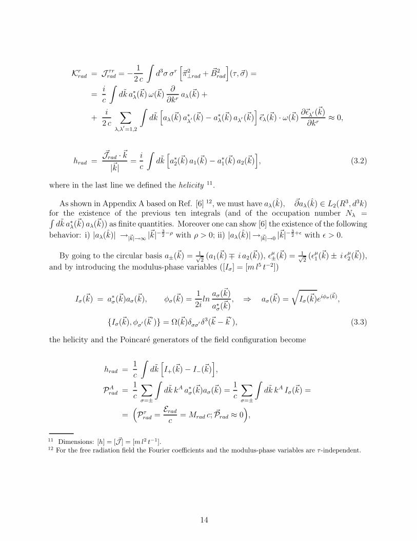
Krrad = J τr

rad = − 1

2 c

∫d3σ σr

[~π2⊥rad + ~B2

rad

](τ, ~σ) =

=i

c

∫dk a∗

λ(~k) ω(~k)

∂

∂kraλ(~k) +

+i

2 c

∑

λ,λ′=1,2

∫dk

[aλ(~k) a∗

λ′ (~k) − a∗

λ(~k) aλ′ (~k)

]~ǫλ(~k) · ω(~k)

∂~ǫλ′ (~k)

∂kr≈ 0,

hrad =~Jrad · ~k|~k|

=i

c

∫dk

[a∗

2(~k) a1(~k) − a∗

1(~k) a2(~k)

], (3.2)

where in the last line we defined the helicity 11.

As shown in Appendix A based on Ref. [6] 12, we must have aλ(k), ~∂aλ(k) ∈ L2(R3, d3k)

for the existence of the previous ten integrals (and of the occupation number Nλ =∫dk a∗

λ(~k) aλ(~k)) as finite quantities. Moreover one can show [6] the existence of the following

behavior: i) |aλ(k)| →|~k|→∞ |~k|− 32−ρ with ρ > 0; ii) |aλ(k)|→|~k|→0 |~k|−

32+ǫ with ǫ > 0.

By going to the circular basis a±(~k) = 1√2(a1(~k)∓ i a2(~k)), ǫµ

±(~k) = 1√2(ǫµ

1 (~k) ± i ǫµ2(

~k)),

and by introducing the modulus-phase variables ([Iσ] = [m l5 t−2])

Iσ(~k) = a∗σ(~k)aσ(~k), φσ(~k) =

1

2iln

aσ(~k)

a∗σ(~k)

, ⇒ aσ(~k) =

√Iσ(~k)eiφσ(~k),

Iσ(~k), φσ′ (~k′

) = Ω(~k)δσσ′ δ3(~k − ~k′

), (3.3)

the helicity and the Poincare generators of the field configuration become

hrad =1

c

∫dk

[I+(~k) − I−(~k)

],

PArad =

1

c

∑

σ=±

∫dk kA a∗

σ(~k)aσ(~k) =1

c

∑

σ=±

∫dk kA Iσ(~k) =

=(Pτ

rad =Erad

c= Mrad c; ~Prad ≈ 0

),

11 Dimensions: [h] = [ ~J ] = [m l2 t−1].12 For the free radiation field the Fourier coefficients and the modulus-phase variables are τ -independent.

14

~Jrad = −1

c

∑

σ

∫dk Iσ(~k)

(~k × ∂

∂ ~k

)φσ(~k) +

+i

2 c

∫dk

[I+(~k) − I−(~k)

][~ǫ+(~k) + ~ǫ−(~k)

]·(~k × ∂

∂ ~k

) [~ǫ−(~k) −~ǫ+(~k)

]+

+i

c

∫dk ~ǫ+(~k) ×~ǫ−(~k)

[I+(~k) − I−(~k)

],

Krrad = −1

c

∑

σ=±

∫dk Iσ(~k)ω(~k)

∂

∂krφσ(k) +

+i

2 c

∫dk

[I+(~k) − I−(~k)

][~ǫ+(~k) + ~ǫ−(~k)

]· ω(~k)

∂

∂kr

[~ǫ−(~k) −~ǫ+(~k)

]≈ 0. (3.4)

As shown in Appendix A and Ref.[6], the existence of finite values of these quantitiesrequires [6] :

i) |Iσ(~k)|→|~k|→∞ |~k|−3−δ with δ > 0; |φσ(~k)|→|~k|→∞ |~k| (this is due to the transformation

properties under Poincare transformations; φ′

σ(~k) = φσ( ~Λ−1 k) + k · a + σ θ(~k, Λ−1));

ii) |Iσ(~k)|→|~k|→0 |~k|−2+ǫ with ǫ > 0; |φσ(~k)|→|~k|→0 |~k|α with α > −δ.

Let us replace the canonical variables Iσ(~k), φσ(~k) with the following new canonical basis

Ψrad(~k), Φrad(~k), λrad(~k), ρrad(~k) 13

Ψrad(~k) =∑

σ=±Iσ(~k), Φrad(~k) =

1

2

∑

σ=±φσ(~k),

λrad(~k) = I+(~k) − I−(~k), ρrad(~k) =1

2

[φ+(~k) − φ−(~k)

],

Ψrad(~k), Φrad(~k′

) = λrad(~k), ρrad(~k′

) = Ω(~k)δ3(~k − ~k′

),

I+(~k) =1

2

(Ψrad(~k) + λrad(~k)

), I−(~k) =

1

2

(Ψrad(~k) − λrad(~k)

),

φ+(~k) = Φrad(~k) + ρrad(~k), φ−(~k) = Φrad(~k) − ρrad(~k), (3.5)

in terms of which the helicity and the Poincare generators become

13 Dimensions: [Ψrad] = [λrad] = [Iσ] = [m l5 t−2].

15

hrad =1

c

∫dk λrad(~k),

PArad =

1

c

∫dk kA Ψrad(~k) =

(Pτ

rad =Erad

c= Mrad c; ~Prad ≈ 0

),

~Jrad = −1

c

∫dk Ψrad(~k)

(~k × ∂

∂ ~k

)Φrad(~k) −

− 1

c

∫dk λrad(~k)

(~k × ∂

∂ ~k

)ρrad(~k) +

+i

2 c

∫dk λrad(~k)

[~ǫ+(~k) + ~ǫ−(~k)

]·(~k × ∂

∂ ~k

) [~ǫ−(~k) −~ǫ+(~k)

]+

+i

c

∫dk λrad(~k)

[~ǫ+(~k) ×~ǫ−(~k)

],

Krrad =

1

c

∫dk Ψrad(~k)ω(k)

∂

∂krΦrad(~k) +

1

c

∫dk λrad(~k)ω(~k)

∂

∂krρrad(~k) +

+i

2 c

∫dk λrad(~k)

[~ǫ+(~k) + ~ǫ−(~k)

]· ω(~k)

∂

∂kr

[~ǫ−(~k) −~ǫ+(~k)

]≈ 0. (3.6)

One has:

i) |Ψ(~k)|→|~k|→0 |~k|−3+ǫ with ǫ > 0; |Φ(~k)|→|~k|→0 |~k|α with α > 1− ǫ; |λrad(~k)|→|~k|→0 |~k|−2−δ

with δ > 0; |ρrad(~k)|→|~k|→0 |~k|β with β > −δ;

ii) |Ψ(~k)|→|~k|→∞ |~k|−3−γ with γ > 0; |Φ(~k)|→|~k|→∞ |~k| ; |λrad(~k)|→|~k|→∞ |~k|−2−χ with

χ > 0; |ρrad(~k)|→|~k|→∞ |~k|β with β > χ.

B. Collective and Relative Variables for the Radiation Field

We can now use the results of Appendix A to replace the canonical variables Ψrad(~k) and

Φrad(~k) with a set of collective and relative canonical variables XArad, PA

φ , Hrad(~k), Krad(~k).

To them must be added the remaining canonical variables λrad(~k) and ρrad(~k) describingthe difference of the modulus-phase variables with different circular polarization (they arealready of the type of relative variables).

By using Eqs.(A6), (A7), (A9) and the function F(~k,PBrad) of Eq.(A8) with ω(k) = k and

with the functions F τ (k), F (k) given in Eqs.(A11), the collective and relative variables are

16

XArad =

∫dk

∂ F(~k,PBφ )

∂ Pφ A

Φrad(~k),

PArad =

1

c

∫dk kA Ψrad(~k) =

∫dk kA F(~k,PB

rad),

Hrad(~k) =

∫dq G(~k, ~q)

[Ψrad(~q) − ω(q) F τ(q)

∫dq1 ω(q1) Ψrad(, ~q1) +

+ F (q) ~q ·∫

dq1 ~q1 Ψrad(~q1)],

Krad(~k) = D~k Φrad(~k),

λrad(~k), ρrad(~k),

XArad,PB

rad = −ηAB,

Hrad(~k),Krad(~k1) = (2π)3 2 ω(k) δ3(~k − ~k1),

λrad(~k), ρrad(~k1) = (2π)3 2 ω(k) δ3(~k − ~k1), (3.7)

with all the other Poisson brackets vanishing. The operator D~q and its Green function aredefined in Ref.[6] and Appendix A. By construction XA

rad is a 4-center of phase.

The helicity and Poincare generators become [Drs = kr ∂∂ks − ks ∂

∂kr , Dτr = ω(k) ∂∂kr ]

hrad =1

c

∫dk λrad(~k),

PArad =

(Pτ

rad =Erad

c= Mrad c; ~Prad ≈ 0

),

~Jrad = ~Srad = ~Xrad × ~Prad + ~Srad,

~Srad = −1

c

∫dk Hrad(~k)

(~k × ∂

∂ ~k

)Krad(~k) −

− 1

c

∫dk λrad(~k)

(~k × ∂

∂ ~k

)ρrad(~k) +

+1

c

∫dk λrad(~k)

[~ǫ−(~k) ×~ǫ+(~k) +

i

2

(~ǫ−(~k) + ~ǫ+(~k)

)· ~k × ∂

∂ ~k

(~ǫ−(~k) −~ǫ+(~k)

)],

Krrad = Xτ

rad Prrad − Xr

rad Mrad c −

− 1

c

∫dk Hrad(~k) Dτr Krad(~k) − 1

c

∫dk λrad(~k) Dτr ρrad(~k) −

− i

2 c

∫dk λrad(~k)

([~ǫ+(~k) + ~ǫ−(~k)

]· Dτr

[~ǫ−(~k) −~ǫ+(~k)

])≈ 0. (3.8)

17

The gauge fixing ~Krad ≈ 0 to the rest-frame conditions ~Prad ≈ 0 leads to the followingdetermination of the 3-center of phase ~Xrad

Xrrad ≈ − 1

Mrad c2

[ ∫dk Hrad(~k) Dτr Krad(~k) +

∫dk λrad(~k) Dτr ρrad(~k) +

+i

2

∫dk λrad(~k)

([~ǫ+(~k) + ~ǫ−(~k)

]· Dτr

[~ǫ−(~k) −~ǫ+(~k)

]) ]. (3.9)

If ~A⊥rad(τ, ~σ) satisfies∫

dk wlm(~k)[Ψrad(~k) − F(~k,PB

rad)]

= 0 for l ≥ 2 (see Ref.[6] and

Appendix A), then we have the following expression of the fields of the transverse radiationfield

~A⊥rad(τ, ~σ) =

∫dk

∑

σ=±

[~ǫσ(~k)

√1

2

(F(~k,PB

rad) + σ λrad(~k))

+ D~k Hrad(~k)

ei[kA (XArad−σA)+σ ρrad(~k)+

R

dk1 dk2 Krad(~k1)G(~k1,~k2)(~k2,~k)] + c.c.],

~π⊥rad(τ, ~σ) = i

∫dk ω(~k)

∑

σ=±

[~ǫσ(~k)

√1

2

(F(~k,PB

rad) + σ λrad(~k))

+ D~k Hrad(~k)

ei[kA (XArad−σA)+σ ρrad(~k)+

R

d k1 dk2 Krad(~k1)G(~k1,~k2)(~k2,~k)] + c.c.],

~Brad(τ, ~σ) = i

∫dk

∑

σ=±

~k ×[~ǫσ(~k)

√1

2

(F(~k,PB

rad) + σ λrad(~k))

+ D~k Hrad(~k)

ei[kA (XArad−σA)+σ ρrad(~k)+

R

d k1 dk2 Krad(~k1)G(~k1,~k2)(~k2,~k)] + c.c.], (3.10)

so that the radiation fields have the following dependence upon τ and ~σ

~A⊥rad(τ, ~σ) = ~A⊥rad(τ − Xτrad, ~σ − ~Xrad),

~π⊥rad(τ, ~σ) = ~π⊥rad(τ − Xτrad, ~σ − ~Xrad),

~Brad(τ, ~σ) = ~Brad(τ − Xτrad, ~σ − ~Xrad), (3.11)

The configurations of the radiation field admitting the collective variables XArad have a

”monopole” structure, carried by ~Xrad and ~prad ≈ 0, plus the ”multipoles” Krad(~k), Hrad(~k),

λrad(~k), ρrad(~k) (these last multipoles describe the helicity structure). Eqs.(3.9) expresses~Xrad in terms of Mrad and of the higher multipoles.

As in the Klein-Gordon case we have the extra variables Xτrad, Pτ

rad = Mrad c with asimilar interpretation (see Appendix A).

By using Eq.(I-2.25) we have the following representation of the potential of the radiation

field: Aµrad

(Y α(τ) + ǫα

r (~h) σr)

= −ǫµr (~h) Ar

⊥rad(τ, ~σ).

18

IV. N CHARGED PARTICLES PLUS THE ELECTRO-MAGNETIC FIELD

Let us now consider the problem of identifying the collective and relative variable for thesystem of two 14 positive-energy charged particles with mutual Coulomb interaction plus anarbitrary electro-magnetic field in the radiation gauge (see Ref.[1] and I). This will allow to

solve the constraints ~K(int) ≈ 0 and to eliminate the internal 3-center of mass like we madein the previous two Sections.

A. The Internal Poincare’ Generators before the Canonical Transformation

From Eq.(I-2.23) we have the following expression of the internal Poincare’ generators in

the original canonical basis ~ηi(τ), ~κi(τ), ~A⊥(τ, ~σ), ~π⊥(τ, ~σ)

E(int) = Pτ(int) c = M c2 = c

∫d3σ T ττ (τ, ~σ) =

= c

2∑

i=1

(√m2

i c2 + ~κ2i (τ) − Qi

c

~κi(τ) · ~A⊥(τ, ~ηi(τ))√m2

i c2 + ~κ2i (τ)

)+

+Q1 Q2

4π | ~η1(τ) − ~η2(τ) | + Eem,

Eem = Pτem c =

1

2

∫d3σ [~π2

⊥ + ~B2](τ, ~σ),

Pr(int) =

∫d3σ T rτ(τ, ~σ) =

2∑

i=1

κri (τ) + Pr

em ≈ 0,

~Pem =1

c

∫d3σ [~π⊥ × ~B](τ, ~σ),

J r(int) = Sr =

1

2ǫruv

∫d3σ σu T vτ (τ, ~σ) =

=2∑

i=1

(~ηi(τ) × ~κi(τ)

)r

+ J rem,

~Jem =1

c

∫d3σ(~σ ×

([~π⊥ × ~B]

)r

(τ, ~σ),

14 The case of N particles follows the same scheme.

19

Kr(int) = −

∫d3σ σr T ττ(τ, ~σ) =

= −2∑

i=1

ηri (τ)

(√m2

i c2 + ~κ2i (τ) − Qi

c

~κi(τ) · ~A⊥(τ, ~ηi(τ))√m2

i c2 + ~κ2i (τ)

)+

+Q1 Q2

4π c

[ ηr1(τ) + ηr

2(τ)

|~η1(τ) − ~η2(τ)| −

−∫

d3σ

4π

( σr − ηr2(τ)

|~σ − ~η1(τ)| |~σ − ~η2(τ)|3 +σr − ηr

1(τ)

|~σ − ~η2(τ)| |~σ − ~η1(τ)|3)]

−

−2∑

i=1

Qi

4π c

∫d3σ

πr⊥(τ, ~σ)

|~σ − ~ηi(τ)| + Krem ≈ 0,

~Kem = − 1

2c

∫d3σ σr (~π2

⊥ + ~B2)(τ, ~σ). (4.1)

For an electro-magnetic field not of the radiation type the quantities Eem, ~Pem, ~Jem, ~Kem

are not conserved and do not satisfy a Lorentz algebra.

In the canonical basis ~A⊥(τ, ~σ), ~π⊥(τ, ~σ), ~ηi(τ), ~κi(τ), it is not clear which are the col-

lective variables to be eliminated by means of the constraints ~P(int) ≈ 0 and ~K(int) ≈ 0,because we do not know how to define these variables for an electro-magnetic field not ofthe radiation type. To treat this type of field we now use results obtained in paper I.

B. The Internal Poincare’ Generators after the Canonical Transformation

After the canonical transformation defined in I, the system is described by a transverse

radiation field ~A⊥rad(τ, ~σ), ~π⊥rad(τ, ~σ), and by Coulomb-dressed particle variables ~ηi(τ),

~κi(τ), see Eqs. (I-3.6) and (I-3.10).

From Eqs.(I-4.4), (I-4.1), (I-4.2), (I-4.6) [and (I-3.9) for Ti and Kij ] we have that eachinternal Poincare’ generator becomes the direct sum of the radiation field one of Eq.(3.2)plus the particle one of Eq.(2.4) [see Eq.(6.46) of Ref.[1]]

E(int) = Pτ(int) c = M c2 = c

2∑

i=1

√m2

i c2 + ~κ2

i (τ) +Q1 Q2

4π | ~η1(τ) − ~η2(τ)|+

+ VDARWIN(~κ1(τ), ~κ2(τ), ~η1(τ) − ~η2(τ)) +

+1

2

∫d3σ

(~π2⊥rad + ~B2

rad

)(τ, ~σ) =

=(Pτ

matter + Pτrad

)c,

20

~P(int) =

2∑

i=1

~κi(τ) +1

c

∫d3σ

(~π⊥rad × ~Brad

)(τ, ~σ) =

= ~Pmatter + ~Prad ≈ 0,

~J(int) =∑

i

~ηi × ~κi +1

c

∫d3σ ~σ ×

(~π⊥rad × ~Brad

)(τ, ~σ) =

= ~Jmatter + ~Jrad,

~K(int) = −2∑

i=1

~ηi

√m2

i c2 + ~κ2

i −

− 1

2

Q1 Q2

c

[~η1

~κ1 ·(

12

∂ K12(~κ1,~κ2,~ρ12)

∂ ~ρ12

− 2 ~A⊥S2(~κ2, ~ρ12))

√m2

1 c2 + ~κ2

1

+

+ ~η2

~κ2 ·(

12

∂ K12(~κ1,~κ2,~ρ12)

∂ ~ρ12

− 2 ~A⊥S1(~κ1, ~ρ12))

√m2

2 c2 + ~κ2

2

]−

− 1

2

Q1 Q2

c

(√m2

1 c2 + ~κ2

1

∂

∂ ~κ1

+

√m2

2 c2 + ~κ2

2

∂

∂ ~κ2

)K12(~κ1, ~κ2, ~ρ12) −

− Q1 Q2

4π c

∫d3σ

( ~π⊥S1(~σ − ~η1, ~κ1)

|~σ − ~η2|+

~π⊥S2(~σ − ~η2, ~κ2)

|~σ − ~η1|

)−

− Q1 Q2

c

∫d3σ ~σ

(~π⊥S1(~σ − ~η1, ~κ1) · ~π⊥S2(~σ − ~η2, ~κ2) +

+ ~BS1(~σ − ~η1, ~κ1) · ~BS2(~σ − ~η2, ~κ2))−

− 1

2 c

∫d3σ ~σ

(~π2⊥rad + ~B2

rad

)(τ, ~σ) =

= ~Kmatter + ~Krad =

def= −1

cE(int)

~R+ = −1

c

(Ematter + Erad

)~R+ ≈ 0. (4.2)

Let us remark that in ~K(int) ≈ 0 of Eq.(4.2) all the particles terms depend on ~ρ12(τ) =

~η1(τ) − ~η2(τ) or ~σ − ~ηi(τ).

21

We also added the connection of ~K(int) with the Møller internal 3-center of energy ~R+15.

Even if all the internal generators are the direct sum of the generators of the two subsys-tems, the two subsystems are connected by the rest-frame conditions and by the vanishing ofthe internal boosts, i.e. by the necessity of eliminating the position and momentum of theinternal overall 3-center of mass.

C. Semi-Relativistic Expansions of E(int) and ~K(int) before and after the Canonical

Transformation

The semi-relativistic limit of the generators E(int) and ~K(int) of Eqs.(4.1) is

E(int) →c→∞ (2∑

i=1

mi) c2 +2∑

i=1

~κ2i (τ)

2mi

+Q1 Q2

4π | ~η1(τ) − ~η2(τ) | −

− 1

c

2∑

i=1

Qi~κi(τ)

mi· ~A⊥(τ, ~ηi(τ)) − 1

c2

2∑

i=1

~κ4i (τ)

8m3i

+

+1

c3

2∑

i=1

Qi~κ2

i (τ)

2m2i

~κi(τ)

mi· ~A⊥(τ, ~ηi(τ)) +

+ O(c−4) +1

2

∫d3σ [~π2

⊥ + ~B2](τ, ~σ),

Kr(int) →c→∞ cKr

Galilei + O(c−1) ≈ 0,

~KGalilei = −N∑

i=1

m1 ~ηi(τ) = −( N∑

i=1

mi

)~x(n) ≈ 0, (4.3)

where ~x(n) is the non-relativistic center of mass, which emerges as the limit of the Møller

internal 3-center of energy ~R+ = −c ~K(int)/E(int). See Section G of paper I for the non-relativistic limit of the relativistic variables ~ηi(τ), ~κi(τ) and of the relativistic external centerof mass.

After the canonical transformation E(int) is given by Eq.(4.2). The semi-relativistic limitof its matter part is

15 We have ~R+ ≈ ~q+ ≈ ~y+ due to the rest-frame condition ~P(int) ≈ 0, where ~q+ is the internal 3-center of

mass and ~y+ the internal Fokker-Pryce 3-center of inertia.

22

Pτmatter =

2∑

i=1

(mi c

2 +~κ

2

i (τ)

2mi

+Q1 Q2

4π |~η1(τ) − ~η2(τ)|− 1

c2

~κ4

i (τ)

8m3i

+

+Q1 Q2

m1 m2 c2

~κ2i (τ) −

[~κi(τ) · ~η1(τ)−~η2(τ)

|~η1(τ)−~η2(τ)|

]2

16π|~η1(τ) − ~η2(τ)|

)+ O(c−4). (4.4)

By using Eqs.(I-2.51) - (I-2.53) for the Lienard-Wiechert fields we get K12 = O(c−3), so

that the semi-relativistic limit of ~K(int) of Eq.(4.2) is

~K(int) = −2∑

i=1

~ηi(τ)(mi c +

~κ2

i

2mic

)+ O(c−2) −

− 1

2c

∫d3σ ~σ

(~π2⊥rad + ~B2

rad

)(τ, ~σ) =

= ~Kmatter + ~Krad = c ~KGalilei + O(1

c) ≈ 0,

~KGalilei = −(m1 + m2) ~x(n) = −2∑

i=1

mi ~ηi ≈ 0 (in the rest frame). (4.5)

D. The Collective Variables after the Canonical Transformation

The results of Section II and III allow us to find the collective and relative variablesof the matter and transverse radiation field subsystems in the canonical basis ~ηi(τ), ~κi(τ),~A⊥ rad(τ, ~σ), ~π⊥ rad(τ, ~σ).

A) The field quantities ~A⊥ rad(τ, ~σ), ~π⊥ rad(τ, ~σ) are canonically equivalent to the canonical

basis Xτrad, Pτ

rad = Mrad c = Erad

c, ~Xrad, ~Prad, λrad(~k), ρrad(~k), Hrad(~k), Krad(~k), given in

Eqs.(3.7), which contains the collective variables for the radiation field.

B) For the particle subsystem we make the canonical transformation (2.3) on theCoulomb-dressed particle variables

~η12 =m1

m~η1 +

m2

m~η2, ~ρ12 = ~η1 − ~η2,

~κ12 = ~κ1 + ~κ2 ≈ 0, ~π12 =m2

m~κ1 −

m1

m~κ2,

~η1 = ~η12 +m2

m~ρ12, ~η2 = ~η12 −

m1

m~ρ12,

~κ1 =m1

m~κ12 + ~π12, ~κ2 =

m2

m~κ12 − ~π12. (4.6)

23

Eqs.(4.2) imply ~Pmatter = ~κ12 ≈ −~Prad = −∫

d3σ (~π⊥rad × ~Brad)(τ, ~σ).

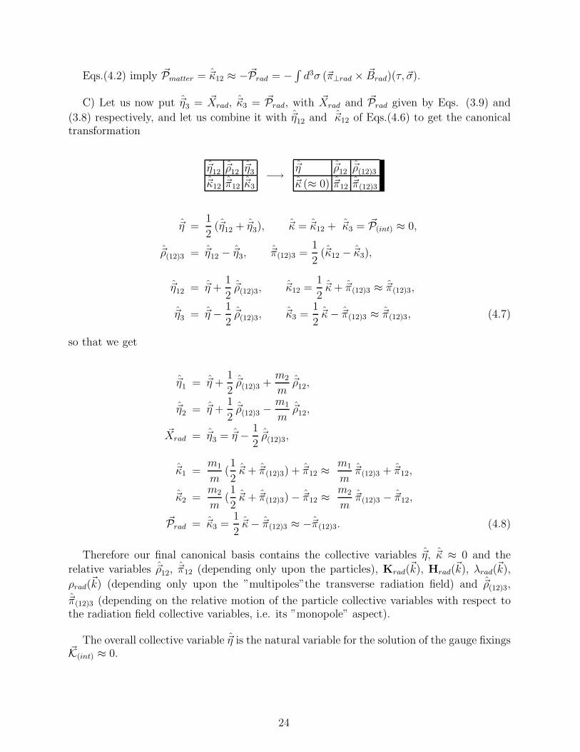
C) Let us now put ~η3 = ~Xrad, ~κ3 = ~Prad, with ~Xrad and ~Prad given by Eqs. (3.9) and

(3.8) respectively, and let us combine it with ~η12 and ~κ12 of Eqs.(4.6) to get the canonicaltransformation

~η12 ~ρ12 ~η3

~κ12 ~π12 ~κ3

−→ ~η ~ρ12 ~ρ(12)3

~κ (≈ 0) ~π12 ~π(12)3

~η =1

2(~η12 + ~η3), ~κ = ~κ12 + ~κ3 = ~P(int) ≈ 0,

~ρ(12)3 = ~η12 − ~η3, ~π(12)3 =1

2(~κ12 − ~κ3),

~η12 = ~η +1

2~ρ(12)3, ~κ12 =

1

2~κ + ~π(12)3 ≈ ~π(12)3,

~η3 = ~η − 1

2~ρ(12)3, ~κ3 =

1

2~κ − ~π(12)3 ≈ ~π(12)3, (4.7)

so that we get

~η1 = ~η +1

2~ρ(12)3 +

m2

m~ρ12,

~η2 = ~η +1

2~ρ(12)3 −

m1

m~ρ12,

~Xrad = ~η3 = ~η − 1

2~ρ(12)3,

~κ1 =m1

m(1

2~κ + ~π(12)3) + ~π12 ≈

m1

m~π(12)3 + ~π12,

~κ2 =m2

m(1

2~κ + ~π(12)3) − ~π12 ≈

m2

m~π(12)3 − ~π12,

~Prad = ~κ3 =1

2~κ − ~π(12)3 ≈ −~π(12)3. (4.8)

Therefore our final canonical basis contains the collective variables ~η, ~κ ≈ 0 and the

relative variables ~ρ12, ~π12 (depending only upon the particles), Krad(~k), Hrad(~k), λrad(~k),

ρrad(~k) (depending only upon the ”multipoles”the transverse radiation field) and ~ρ(12)3,

~π(12)3 (depending on the relative motion of the particle collective variables with respect tothe radiation field collective variables, i.e. its ”monopole” aspect).

The overall collective variable ~η is the natural variable for the solution of the gauge fixings~K(int) ≈ 0.

24

E. The Internal 3-Center of Mass ~η from the vanishing of the Internal Boosts after

the Canonical Transformation.

We have to find ~η of Eq.(4.7) from the vanishing of the internal boosts ~K(int) ≈ 0 in theform (4.2), put it into Eqs.(4.8 ) and make the inverse canonical transformation (I-3.10) tofind the original ~ηi(τ) and the particle world-lines xµ

i (τ) like we made in Eqs.(2.8).

In the boosts in the form (4.2) the first four lines of the particle terms depend on ~ρ12 =

~η1− ~η2 and ~π12 = m2

m~κ1− m1

m~κ2, but they also get a dependence on ~π(12)3 = 1

2(~κ1+~κ2− ~Prad)

through the dependence on the particle momenta. In the next two particle terms we must

shift the integration variable to reabsorb the quantity ~η + 12~ρ(12)3 present in ~σ − ~ηi.

Finally the last line of the boosts in Eqs.(4.2) is just ~Krad of Eqs.(3.8).

Therefore the internal boosts in the form (4.2) has the following form in the new canonical

basis (~κi(τ) are given by Eqs.(4.8))

~K(int) = −(~η +

1

2~ρ(12)3

)( 2∑

i=1

√m2

i c2 + ~κ2

i +1

2

Q1 Q2

c×

×[~κ1 ·

(12

∂ K12(~κ1,~κ2,~ρ12)

∂ ~ρ12

− 2 ~A⊥S2(~κ2, ~ρ12))

√m2

1 c2 + ~κ2

1

+

+~κ2 ·

(12

∂ K12(~κ1,~κ2,~ρ12)

∂ ~ρ12

− 2 ~A⊥S1(~κ1, ~ρ12))

√m2

2 c2 + ~κ2

2

])−

− ~ρ12

(m2

m

√m2

1 c2 + ~κ2

1 −m1

m

√m2

2 c2 + ~κ2

2 +

+1

2

Q1 Q2

c

[m2

m

~κ1 ·(

12

∂ K12(~κ1,~κ2,~ρ12)

∂ ~ρ12

− 2 ~A⊥S2(~κ2, ~ρ12))

√m2

1 c2 + ~κ2

1

−

25

− m1

m

~κ2 ·(

12

∂ K12(~κ1,~κ2,~ρ12)

∂ ~ρ12

− 2 ~A⊥S1(~κ1, ~ρ12))

√m2

2 c2 + ~κ2

2

])−

− 1

2

Q1 Q2

c

(√m2

1 c2 + ~κ2

1

∂

∂ ~κ1

+

√m2

2 c2 + ~κ2

2

∂

∂ ~κ2

)K12(~κ1, ~κ2, ~ρ12) −

− Q1 Q2

4π c

∫d3σ

( ~π⊥S1(~σ − m2

m~ρ12, ~κ1)

|~σ + m1

m~ρ12|

+~π⊥S2(~σ + m1

m~ρ12, ~κ2)

|~σ − m2

m~ρ12|

)−

− Q1 Q2

c

∫d3σ

[~σ + ~η +

1

2~ρ(12)3

] (~π⊥S1(~σ − m2

m~ρ12, ~κ1) · ~π⊥S2(~σ +

m1

m~ρ12, ~κ2) +

+ ~BS1(~σ − m2

m~ρ12, ~κ1) · ~BS2(~σ +

m1

m~ρ12, ~κ2)

)−

− Xτrad ~π(12)3 − Mrad c

(~η − 1

2~ρ(12)3

)+ ~D(Hrad,Krad, λrad, ρrad) ≈ 0,

(4.9)

where the term ~D(Hrad,Krad, λrad, ρrad) has the following expression

Dr(Hrad,Krad, λrad, ρrad) = −1

c

∫dk Hrad(~k) Dor Krad(~k) − 1

c

∫dk λrad(~k) Dor ρrad(~k) −

− i

2c

∫dk λrad(~k)

[~ǫ+(~k) + ~ǫ−(~k)

]· Dor

[~ǫ−(~k) −~ǫ+(~k)

]. (4.10)

The solution of Eq.(4.9) is

~η ≈ 1

A + Mrad c

(− 1

2(A− Mrad c) ~ρ(12)3 −

−[m2

m

√m2

1 c2 + (~π12 +m1

m~π(12)3)2 − m1

m

√m2

2 c2 + (~π12 −m2

m~π(12)3)2 + B

]~ρ12 − ~C +

+ Xτrad ~π(12)3 + ~D

), (4.11)

where we have introduced the following definitions (~κi(τ) are given by Eqs.(4.8))

26

A(~ρ12, ~π12, ~π(12)3) =2∑

i=1

√m2

i c2 + ~κ2

i +1

2

Q1 Q2

c×

×[~κ1 ·

(12

∂ K12(~κ1,~κ2,~ρ12)

∂ ~ρ12

− 2 ~A⊥S2(~κ2, ~ρ12))

√m2

1 c2 + ~κ2

1

+

+~κ2 ·

(12

∂ K12(~κ1,~κ2,~ρ12)

∂ ~ρ12

− 2 ~A⊥S1(~κ1, ~ρ12))

√m2

2 c2 + ~κ2

2

]−

− Q1 Q2

c

∫d3σ

(~π⊥S1(~σ − m2

m~ρ12, ~κ1) · ~π⊥S2(~σ +

m1

m~ρ12, ~κ2) +

+ ~BS1(~σ − m2

m~ρ12, ~κ1) · ~BS2(~σ +

m1

m~ρ12, ~κ2)

),

B(~ρ12, ~π12, ~π(12)3) =1

2

Q1 Q2

c

[m2

m

~κ1 ·(

12

∂ K12(~κ1,~κ2,~ρ12)

∂ ~ρ12

− 2 ~A⊥S2(~κ2, ~ρ12))

√m2

1 c2 + ~κ2

1

−

− m1

m

~κ2 ·(

12

∂ K12(~κ1,~κ2,~ρ12)

∂ ~ρ12

− 2 ~A⊥S1(~κ1, ~ρ12))

√m2

2 c2 + ~κ2

2

],

~C(~ρ12, ~π12, ~π(12)3) = −1

2

Q1 Q2

c

(√m2

1 c2 + ~κ2

1

∂

∂ ~κ1

+

√m2

2 c2 + ~κ2

2

∂

∂ ~κ2

)K12(~κ1, ~κ2, ~ρ12) −

− Q1 Q2

4π c

∫d3σ

( ~π⊥S1(~σ − m2

m~ρ12, ~κ1)

|~σ + m1

m~ρ12|

+~π⊥S2(~σ + m1

m~ρ12, ~κ2)

|~σ − m2

m~ρ12|

)−

− Q1 Q2

c

∫d3σ ~σ

(~π⊥S1(~σ − m2

m~ρ12, ~κ1) · ~π⊥S2(~σ +

m1

m~ρ12, ~κ2) +

+ ~BS1(~σ − m2

m~ρ12, ~κ1) · ~BS2(~σ +

m1

m~ρ12, ~κ2)

). (4.12)

Since, as shown in Eqs.(4.2), we have ~K(int) = c ~KGalilei + O(1c) ≈ 0 we have ~η =

~x(n) + O(c−2) ≈ 0 in the non-relativistic limit, namely we get the non-relativistic rest frame~KGalilei = −m~x(n) = −∑2

i=1 mi ~ηi ≈ 0.

By using Eqs. (4.11), (3.8), (4.8) and the rest-frame condition ~P(int) = ~κ(τ) ≈ 0, weget the following expressions of the internal invariant mass and of the internal angularmomentum in Eqs.(4.2)

27

E(int) = M c2 ≈ Mrad c2 +

+ c

√m2

1 c2 + (~π12 +m1

m~π(12)3)2 + c

√m2

2 c2 + (~π12 −m2

m~π(12)3)2 +

+Q1 Q2

4π |~ρ12|+ VDARWIN(~ρ12; ~π12 +

m1

m~π(12)3;−~π12 +

m2

m~π(12)3),

Mrad c2 =1

2

∫d3σ

[~π2⊥rad + ~B2

rad

](τ, ~σ), (4.13)

~J(int) = ~S ≈ ~ρ12 × ~π12 + ~ρ(12)3 × ~π(12)3 + ~Srad,

~Srad = −1

c

∫dk Hrad(~k)~k × ∂

∂ ~kKrad(~k) − 1

c

∫dk λrad(~k)~k × ∂

∂ ~kρrad(~k) +

+1

c

∫dk λrad(~k)

[~ǫ−(~k) ×~ǫ+(~k) +

i

2

(~ǫ−(~k) + ~ǫ+(~k)

)· ~k × ∂

∂ ~k

(~ǫ−(~k) −~ǫ+(~k)

)].

(4.14)

Eqs.(4.7), (4.8) and (4.9) imply

~η12 = ~η +1

2~ρ(12)3 ≈ 1

A + Mrad c

(Mrad c ~ρ(12)3 −

−[m2

m

√m2

1 c2 + (~π12 +m1

m~π(12)3)2 − m1

m

√m2

2 c2 + (~π12 −m2

m~π(12)3)2 + B

]~ρ12 −

− ~C + Xτrad ~π(12)3 + ~D

),

~η1 ≈ 1

A + Mrad c

(Mrad c ~ρ(12)3 +

[m2

m

(A + Mrad c −

√m2

1 c2 + (~π12 +m1

m~π(12)3)2

)+

+m1

m

√m2

2 c2 + (~π12 −m2

m~π(12)3)2 + B

]~ρ12 − ~C + Xτ

rad ~π(12)3 + ~D),

~η2 ≈ 1

A + Mrad c

(Mrad c ~ρ(12)3 −

[m2

m

√m2

1 c2 + (~π12 +m1

m~π(12)3)2 +

m1

m

(A + Mrad c −

−√

m22 c2 + (~π12 −

m2

m~π(12)3)2

)+ B

]~ρ12 − ~C + Xτ

rad ~π(12)3 + ~D).

(4.15)

These equations, together with the inverse canonical transformation (I-3.10) and by usingEqs.(I-2.51), (I-2.52), (I-3.9), (3.8) and (4.8), allow to get the original variables ~ηi(τ) andthe world-lines (I-2.18) of the particles only in terms of relative variables

28

xµ1 (τ) = Y µ(τ) + ǫµ

r (~h) ηr1,

xµ2 (τ) = Y µ(τ) + ǫµ

r (~h) ηr2,

ηr1(τ) ≈ ηr

1(τ) − Q1

c

m

m1

∂

∂ π(12)3 r

∫d3σ

[~π⊥rad

(τ − Xτ

rad, ~σ +1

2~ρ(12)3

)·

· ~A⊥S1

(~σ − 1

2~ρ(12)3 −

m2

m~ρ12,

m1

m~π(12)3 + ~π12

)−

− ~A⊥rad

(τ − Xτ

rad, ~σ +1

2~ρ(12)3

)·

·~π⊥S1

(~σ − 1

2~ρ(12)3 −

m2

m~ρ12,

m1

m~π(12)3 + ~π12

)]−

− Q1 Q2

2 c

m

m1

∂

∂ π(12)3 r

∫d3σ

[~A⊥S1

(~σ − 1

2~ρ(12)3 −

m2

m~ρ12,

m1

m~π(12)3 + ~π12

)·

·~π⊥S2

(~σ − 1

2~ρ(12)3 +

m1

m~ρ12,

m2

m~π(12)3 − ~π12

)−

− ~π⊥S1

(~σ − 1

2~ρ(12)3 −

m2

m~ρ12,

m1

m~π(12)3 + ~π12

)·

· ~A⊥S2

(~σ − 1

2~ρ(12)3 +

m1

m~ρ12,

m2

m~π(12)3 − ~π12

)],

ηr2(τ) ≈ ηr

2(τ) − Q2

c

m

m2

∂

∂ π(12)3 r

∫d3σ

[~π⊥rad

(τ − Xτ

rad, ~σ +1

2~ρ(12)3

)·

· ~A⊥S2

(~σ − 1

2~ρ(12)3 +

m1

m~ρ12,

m2

m~π(12)3 − ~π12

)−

− ~A⊥rad

(τ − Xτ

rad, ~σ +1

2~ρ(12)3

)·

·~π⊥S2

(~σ − 1

2~ρ(12)3 +

m1

m~ρ12,

m2

m~π(12)3 − ~π12

)]+

+Q1 Q2

2 c

m

m2

∂

∂ π(12)3 r

∫d3σ

[~A⊥S1

(~σ − 1

2~ρ(12)3 −

m2

m~ρ12,

m1

m~π(12)3 + ~π12

)·

·~π⊥S2

(~σ − 1

2~ρ(12)3 +

m1

m~ρ12,

m2

m~π(12)3 − ~π12

)−

− ~π⊥S1

(~σ − 1

2~ρ(12)3 −

m2

m~ρ12,

m1

m~π(12)3 + ~π12

)·

· ~A⊥S2

(~σ − 1

2~ρ(12)3 +

m1

m~ρ12,

m2

m~π(12)3 − ~π12

)],

(4.16)

F. The Final Relative Canonical Variables

The final independent canonical relative variables are

29

a) ~ρ12(τ), ~π12(τ) (relative motion of the two particles);

b) ~ρ(12)3(τ), ~π(12)3(τ) (relative motion of the ”particle system” with respect to the ”radi-ation field system”);

c) Xτrad(τ), Pτ

rad(τ) = 1cErad(τ) = Mrad(τ) c (the energy of the radiation field and its

conjugate temporal variable, the only surviving collective variables);

d) Hrad(~k), Krad(~k) (relative multipoles of the radiation field with respect to its monopole-like collective variables);

e) λrad(~k), ρrad(~k) (relative variables describing the helicity degrees of freedom of theradiation field).

These variables satisfy Hamilton equations having E(int) of Eq.(4.13) as Hamiltonian.

There are the following constants of motion:

A) The relative 3-momentum ~π(12)3 = 12

(~κ1 + ~κ2 − ~Prad

)≈ −~Prad ≈ ~κ1 + ~κ2:

~π(12)3, E(int) = 0.

The constant of the motion ~π(12)3 connects the particles and the radiation field. Itsconjugate variable satisfies the kinematical Hamilton equation

d ~ρ(12)3(τ)

d τ=

∂ E(int)

∂ ~π(12)3

= cm1

m

~π12 + m1

m~π(12)3√

m21 c2 + (~π12 + m1

m~π(12)3)2

+

+ cm2

m

~π12 − m2

m~π(12)3√

m22 c2 + (~π12 − m2

m~π(12)3)2

+

+∂ VDARWIN(~ρ12; ~π12 + m1

m~π(12)3;−~π12 + m2

m~π(12)3)

∂ ~π(12)3

. (4.17)

B) The energy of the radiation field: Pτrad, E(int) = 0. Its conjugate variable Xτ

rad(τ),Xτ

rad,Pτrad = −1, satisfies

d Xτrad

d τ= Xτ

rad, E(int) = −1. (4.18)

Like for the Klein-Gordon case of Appendix A, the two second class constraints Pτrad −

Erad ≈ 0, Xτrad − τ ≈ 0, eliminating the last two collective variables, select a symplectic

sub-manifold of the surface of constant energy Pτrad = Erad of the radiation field.

C) The multipoles Hrad(~k), Krad(~k), λrad(~k), ρrad(~k).

Therefore the two subsystems (particles and radiation field), although not coupled in theequations of motion due to E(int) = Ematter + Erad, are nevertheless effectively interactingthrough the rest-frame constraints and their gauge fixings as clear from Eq.(4.17).

30

The canonical variables ~q+, ~κ+ = ~κ12, ~ρq, ~πq, describing the canonical (Coulomb-dressed)Newton-Wigner 3-center of mass and the relative motion of the 2-particle subsystem (seeSubsection IIA), could be found by using Eqs.(4.7) and (4.8). Then we could re-express

E(int) of Eq.(4.13) and ~J(int) of Eq.(4.14) in terms of them. In particular these variableswould allow to write E(int) of Eq.(4.13) in the form

E(int) ≈ c

√M2

o c2 + ~π2

(12)3 +(function of ~ρq, ~πq, ~π(12)3....

)+ Pτ

rad,

Mo c =

√m2

1 c2 + ~π2

q +

√m2

2 c2 + ~π2

q . (4.19)

In this way the 2-particle subsystem is visualized as an effective pseudo-particle (an atom

after quantization) of mass Mo plus interactions. However a drawback of these variables

is that the Coulomb interaction depends upon ~ρ12 and not upon ~ρq, variables which do not

coincide for ~κ 6= 0.

G. Coming back with the Inverse Canonical Transformation

If we use the inverse canonical transformation (I-3.10) of I, Eqs.(4.7)-(4.8) and the con-

sequences (4.11)-(4.15) of ~K(int) ≈ 0, we can get the expression of ~Pem, ~Jem and Pτem of

Eqs.(4.1) in terms of the radiation field and of the Coulomb-dressed particles from the com-parison of the internal Poincare’ generators before and after the canonical transformation.

Eqs. (4.1) and (4.2) imply

~Pem =1

c

∫d3σ

(~π⊥ × ~B

)(τ, ~σ) ≈

≈ ~Prad −2∑

i=1

Qi

c

∂ Ti(τ)

∂ ~ηi

− 1

2

Q1 Q2

c

( ∂

∂ ~η1

− ∂

∂ ~η2

)K12(τ) =

=1

c

∫d3σ

(~π⊥rad × ~Brad

)(τ, ~σ) + O(

1

c) ≈

≈ −~π(12)3 + O(1

c),

(4.20)

31

~Jem =1

c

∫d3σ ~σ ×

(~π⊥ × ~B

)(τ, ~σ) ≈

≈ ~Srad −(~η − 1

2~ρ(12)3

)× ~π(12)3 −

−2∑

i=1

Qi

c

(~ηi ×

∂ Ti(τ)

∂ ~ηi

+ ~κi ×∂ Ti(τ)

∂ ~κi

)−

−1

2

Q1 Q2

c

2∑

i=1

(~ηi ×

∂ K12(τ)

∂ ~ηi

+ ~κi ×∂ K12(τ)

∂ ~κi

)=

= ~Srad + O(1

c), (4.21)

Pτem =

1

2 c

∫d3σ

(~π2⊥ + ~B2

)(τ, ~σ) =

= Pτrad +

2∑

i=1

(√m2

i c2 +(mi

m~π(12)3 + (−)i+1 ~π12

)2

−√

m2i c2 + ~κ2

i

)+

+Q1 Q2

4π c |~ρ12|− Q1 Q2

4π c |~ρ12|+

1

cVDarwin(~ρ12, ~π12, ~π(12)3) +

+

2∑

i=1

Qi

c

~κi · ~A⊥(τ, ~ηi(τ))√m2

i c2 + ~κ2i

=

=1

2 c

∫d3σ

(~π2⊥rad + ~B2

rad

)(τ, ~σ) + O(

1

c2). (4.22)

This is in accord with Eq.(I-2.49) whose semi-relativistic limit aem λ(τ,~k) =

aλ(~k) e−i ω(~k) τ +ω(~k)~ǫλ(~k)·∑2i=1

Qi

mi ce−i~k·~ηi(τ)

~k4~k ×

(~κi(τ) × ~k

)+O(c−3) says the Fourier coef-

ficients of the transverse electro-magnetic field differ from those of a transverse radiation fieldfor particle terms of order O(c−1). This is the error when we replace the electro-magneticfield with a radiation field, as is often done in atomic physics.

32

V. THE MULTIPOLAR EXPANSION OF THE PARTICLE ENERGY-

MOMENTUM TENSOR

As said in Section I of paper I, in the rest-frame instant form the isolated system ofcharged particles plus the transverse electro-magnetic field can be described as a decouplednon-covariant center of mass carrying the invariant mass and the spin of the isolated system,i.e. some type of pole-dipole structure. The invariant mass and the spin are evaluated bymeans of the energy-momentum tensor TAB(τ, ~σ) = TAB

matter(τ, ~σ)+TABem (τ, ~σ) determined by

using the action (I-2.1) of the parametrized Minkowski theory.

Let us now consider the open subsystem composed only by the particles, whose non-conserved energy-momentum tensor is TAB

matter(τ, ~σ). The study of its multipolar expansion(see Ref.[11]) allows one to replace the extended subsystem with its multipoles when someanalyticity conditions are satisfied and then to define a pole-dipole approximation of thesubsystem. As shown in Ref.[11], this can be done also for single strongly bound groups ofparticles, to be used to describe atoms after quantization, inside the particle subsystem byidentifying the effective energy-momentum of each group.

Till now this is the only description of a relativistic (either free or interacting with theenvironment) composite system like an atom as a collective point-like system endowed withmultipolar properties. The lowest approximation of the composite system is the pole-dipoleapproximation, in which the system is simulated with a point-like particle (monopole) ofmass Mc moving along the world-line of an effective 4-center of motion and carrying thespin dipole ~Jc (to be used for the magnetic dipole moment). In the rest-frame instant form

the 4-center of motion has the world-line wµc (τ) = Y µ(τ) + ǫµ

r (~h) ζrc (τ) and 4-momentum

P µc = hµ Mc c + ǫµ

r (~h)Prc .

Let us remark that this pole-dipole approximation is not the ”dipole approximation” ofthe semi-relativistic atomic physics, which will be studied in the next Section.

As shown in Ref.[11], given a non-isolated cluster of particles the main problem is thedetermination of an effective 4-center of motion described by 3-coordinates ζr

c (τ) and with

world-line wµc (τ) = Y µ(τ)+ǫµ

r (~h) ζrc (τ) in the rest frame of the isolated system 16. The unit 4-

velocity of this center of motion is uµc (τ) = wµ

c (τ)/

√1 − ~ζ

2

c(τ) with wµc (τ) = hµ + ǫµ

r (~h) ζrc (τ)

(from paper I we have hµ = uµ(P ) = P µ/Mc). By using δ zµ(τ, ~σ) = ǫµr (~h) (σr − ζr(τ)) we

can define the Dixon multipoles of the cluster with respect to the world-line wµc (τ)

qr1..rnABc (τ) =

∫d3σ [σr1 − ζr1

c (τ)]..[σrn − ζrnc (τ)] TAB

matter(τ, ~σ). (5.1)

The mass and momentum monopoles, and the mass, momentum and spin dipoles are,respectively

16 See Ref. [11] for a discussion of the main choices present in the literature.

33

qττc = Mc, qrτ

c = Prc ,

qrττc = −Kr

c − Mc ζrc (τ) = Mc (Rr

c(τ) − ζrc (τ)), qruτ

c = pruc (τ) − ζr

c (τ)Puc ,

pruc =

∫d3σ σr T uτ

matter(τ, ~σ) =

2∑

i=1

ηri (τ) κu

i (τ) −

−2∑

i=1

Qi

∫d3σ c(~σ − ~ηi(τ))

(∂r Au

⊥ + ∂u Ar⊥

)(τ, ~σ),

pruc + pur

c =2∑

i=1

(ηr

i (τ) κui (τ) + ηu

i (τ) κri (τ)

)−

− 22∑

i=1

Qi

∫d3σ c(~σ − ~ηi(τ))

(∂r Au

⊥ + ∂u Ar⊥

)(τ, ~σ)

pruc − pur

c

def= ǫruv J v

c ,

Sµνc = [ǫµ

r (~h) hν − ǫνr (

~h) hµ] qrττc + ǫµ

r (~h) ǫνu(

~h) (qruτc − qurτ

c ) =

= [ǫµr (~h) hν − ǫν

r (~h) hµ] Mc (Rr

c − ζrc ) +

+ ǫµr (~h) ǫν

u(~h)

[ǫruv J v

c − (ζrc Pu

c − ζuc Pr

c )],

⇒ mµc(P ) = −Sµν

c hν = −ǫµr (~h) qrττ

c , (5.2)

where ~Jc and ~Kc are the angular momentum and the boost associated with the chosendefinition of effective center of motion.

As shown in Ref.[11], it is convenient to choose the center of energy ~Rc = −~Kc/Mc c

as center of motion. ~Rc and ~Pc (momentum monopole) are the non-canonical variablesdescribing the monopole, i.e. the collective pseudo-particle of non-conserved mass Mc (massmonopole).

On the world-line of this collective pseudo-particle there is also a spin dipole (the anti-symmetric part of the momentum dipole) and the symmetric part of the momentum dipole17. See Ref.[11], Eqs. (5.23) - (5.26).

Since we are in a Hamiltonian formulation, the constitutive relation between monopole

3-velocity d ~ζc(τ)d τ

and monopole (non conserved) 3-momentum ~Pc must not be added by hand,but can be determined for each choice of collective center of motion [11].

As shown in Ref.[11], the total 4-momentum P µc = ǫµ

A(~h) qAτc = hµ Mo + ǫµ

r (~h)Prc and the

spin dipole tensor Sµνc obey the Papapetrou-Dixon-Souriau equations.

17 This symmetric part of the momentum dipole depends on the electromagnetic potential and is connected

with the electric dipole: it is directed along the associated relative momentum if one introduces a suitable

definition of a relative variable.

34

A. The Multipolar Expansion after the Canonical Transformation.

Let us consider the open subsystem formed by the particles.

From Eqs.(4.13) and (4.14) we get

Ematter(τ) = c

√m2

1 c2 + (~π12 +m1

m~π(12)3)2 + c

√m2

2 c2 + (~π12 −m2

m~π(12)3)2 +

+Q1 Q2

4π |~ρ12|+ VDARWIN(~ρ12; ~π12 +

m1

m~π(12)3;−~π12 +

m2

m~π(12)3)

= constant,

~Pmatter(τ) =

2∑

i=1

~κi(τ) ≈ ~π(12)3= constant,

~Jmatter(τ) =∑

i

~ηi(τ) × ~κi(τ) = ~ρ12 × ~π12 +(~η +

1

2~ρ(12)3

)× ~π(12)3

= constant,

(5.3)

while from Eq.(4.2) we get

~Kmatter = −2∑

i=1

~ηi

√m2

i c2 + ~κ2

i −

− 1

2

Q1 Q2

c

[~η1

~κ1 ·(

12

∂ K12(~κ1,~κ2,~ρ12)

∂ ~ρ12

− 2 ~A⊥S2(~κ2, ~ρ12))

√m2

1 c2 + ~κ2

1

+

+ ~η2

~κ2 ·(

12

∂ K12(~κ1,~κ2,~ρ12)

∂ ~ρ12

− 2 ~A⊥S1(~κ1, ~ρ12))

√m2

2 c2 + ~κ2

2

]−

− 1

2

Q1 Q2

c

(√m2

1 c2 + ~κ2

1

∂

∂ ~κ1

+

√m2

2 c2 + ~κ2

2

∂

∂ ~κ2

)K12(~κ1, ~κ2, ~ρ12) −

− Q1 Q2

4π c

∫d3σ

( ~π⊥S1(~σ − ~η1, ~κ1)

|~σ − ~η2|+

~π⊥S2(~σ − ~η2, ~κ2)

|~σ − ~η1|

)−

− Q1 Q2

c

∫d3σ ~σ

(~π⊥S1(~σ − ~η1, ~κ1) · ~π⊥S2(~σ − ~η2, ~κ2) +

+ ~BS1(~σ − ~η1, ~κ1) · ~BS2(~σ − ~η2, ~κ2))

=

def= −1

cEmatter

~Rc(τ). (5.4)

While the natural choice for the effective center of motion is center of energy ~ζc = ~Rc =

−c~Kmatter

Ematter, Eq.(5.3) suggests the other possibility ~ζmatter(τ) = ~η12 = ~η + 1

2~ρ(12)3 with ~η given

35

in Eq.(4.11): it would imply the relation ~Jmatter(τ) = ~ρ12 × ~π12 + ~ζmatter(τ) × ~π(12)3 and ,

differently from the choice ~ζc = ~Rc, ~ζmatter is a canonical variable like ~η12 (however ~π(12)3 isnot the conjugate variable).

36

VI. THE DIPOLE APPROXIMATION OF ATOMIC PHYSICS

Let us now look for the relativistic generalization of the electric dipole approximation ofsemi-relativistic atomic physics. To this end we consider a 2-particle system and we replacethe particle 3-positions ~ηi and 3-momenta ~κi, i = 1, 2, with the naive center of mass andrelative variables of Eqs. (2.3): ~η12, ~κ12, ~ρ12, ~π12.

The standard electric dipole moment is directed along the relative variable ~ρ12. Usuallyonly neutral systems with opposite charges of the particles are considered in applicationsof the dipole approximation. As a consequence it is convenient to introduce the followingnotation for the Grassmann-valued charges

Q1 = Q + Q, Q2 = −Q + Q, Q21 = Q2

2 = 0, Q1 Q2 = Q2 Q1 6= 0,

Q =1

2(Q1 − Q2), Q =

1

2(Q1 + Q2), Q2 = −Q1 Q2, Q2 = Q1 Q2 if Q 6= 0.

(6.1)

The restriction to opposite charges is done by introducing the constraint Q ≈ 0, whichimplies e = Q ≈ Q1 ≈ −Q2. This allows us to discard the terms in Q1 Q2 coming from Q2

from those coming from Q2: only these terms will produce effects of order e2 in a neutralsystem with Grassmann regularization (it eliminates the e2 terms coming from Q2

1 and Q22).

Strictly speaking it is only after the quantization of the Grassmann-valued charges Qi,sending each of them in a two-level system with charges (+e, 0) or (−e, 0), that we are reallyallowed to use e = Q1 = −Q2.

The natural definition of a Grassmann-valued electric dipole moment is

~d(τ) = Q ~ρ12(τ) =Q1 − Q2

2~ρ12(τ) →e=Q1≈−Q2 e ~ρ12(τ). (6.2)

The alternative definition

~D(τ) =2∑

i=1

Qi ~ηi(τ) = ~d(τ) + 2Q[~η12(τ) +

m2 − m1

2m~ρ12(τ)

]→Q≈0

~d(τ), (6.3)

is equivalent to Eq.(6.2) for neutral systems.

The electric dipole has not to be confused with the Dixon spin dipole, which is orientedalong the spin ~S = ~ρ12 × ~π12 and determines the direction of the magnetic dipole moment.

The length |~ρ12(τ)| is of the size of the atom, i.e. a few Bohr radii. For a monochro-

matic electromagnetic wave, i.e. for ~A⊥(τ, ~η12(τ)) ≈ ~a ei~k·~η12(τ) with |~k| = 2πλem

, we have

1

| ~A⊥(τ,~η12(τ))| |(~ρ12(τ) · ∂

∂ ~η12

)~A⊥(τ, ~η12(τ))| ≈ ~ρ12(τ) ·~k ≈ 2π size of atom

λem. This ratio is << 1 in

the long wavelength approximation λem >> size of atom (i.e. for radio-frequency, infrared,visible or ultraviolet radiation).

37

To get the dipole approximation [7] we use Eq.(2.3) and we make the following expansion(m3 ≡ m1)

~A⊥(τ, ~ηi(τ)) = ~A⊥

(τ, ~η12(τ) + (−)i+1 mi+1

m~ρ12(τ)

)=

= ~A⊥(τ, ~η12(τ)) + (−)i+1 mi+1

m

(~ρ12(τ) · ∂

∂ ~η12

)~A⊥(τ, ~η12(τ)) +

+ O([~ρ12 · ~∂~η12 ]2 ~A⊥). (6.4)

For the internal Poincare’ energy generator of Eqs.(4.1) we have (µ = m1 m2/m)

E(int) = M c2 =

= c(√

m21 c2 +

(m1

m~κ12(τ) + ~π12(τ)

)2

+

√m2

2 c2 +(m2

m~κ12(τ) − ~π12(τ)

)2)−

−( m1 Q1√

m21 c2 +

(m1

m~κ12(τ) + ~π12(τ)

)2+

m2 Q2√m2

2 c2 +(

m2

m~κ12(τ) − ~π12(τ)

)2

)

~κ12(τ)

m· ~A⊥(τ, ~η12(τ)) −

−( Q1√

m21 c2 +

(m1

m~κ12(τ) + ~π12(τ)

)2− Q2√

m22 c2 +

(m2

m~κ12(τ) − ~π12(τ)

)2

)

~π12(τ) · ~A⊥(τ, ~η12(τ)) −

− µ

m

( Q1√m2

1 c2 +(

m1

m~κ12(τ) + ~π12(τ)

)2− Q2√

m22 c2 +

(m2

m~κ12(τ) − ~π12(τ)

)2

)

~κ12 ·(~ρ12(τ) · ∂

∂ ~η12

)~A⊥(τ, ~η12(τ)) −

−( m2 Q1√

m21 c2 +

(m1

m~κ12(τ) + ~π12(τ)

)2+

m1 Q2√m2

2 c2 +(

m2

m~κ12(τ) − ~π12(τ)

)2

)

~π12(τ)

m·(~ρ12(τ) · ∂

∂ ~η12

)~A⊥(τ, ~η12(τ)) +

+Q1 Q2

4π |~ρ12(τ)| +1

2

∫d3σ [~π2

⊥ + ~B2](τ, ~σ) + O([~ρ12 · ~∂~η12 ]2 ~A⊥). (6.5)

38

Its semi-relativistic limit with the restriction e = Q1 ≈ −Q2 is

E(int) →c→∞,e=Q1≈Q2 mc2 +~κ2

12(τ)

2m+

~π212(τ)

2µ− e2

4π |~ρ12(τ)| −

− e

c

~π12(τ)

µ· ~A⊥(τ, ~η12(τ)) −

− e

c

~κ12(τ)

m·(~ρ12(τ) · ∂

∂ ~η12

)~A⊥(τ, ~η12(τ)) −

− e

c

m2 − m1

m

~π12(τ)

µ·(~ρ12(τ) · ∂

∂ ~η12

)~A⊥(τ, ~η12(τ)) +

+ O(c−2) + O([~ρ12 · ~∂~η12 ]2 ~A⊥).

(6.6)

In this way we recover a semi-classical version of Eqs.(L3), (L4) and (14.34) of Ref. [7],without the e2 terms corresponding to Q2

i = 0.

If we could evaluate the internal 3-center of mass ~q+ (see Subsection IIA) as a functionof ~η12, ~κ12 = ~κ+, ~ρ12, ~π12, then the results of Section IV would allow us to write the internalPoincare’ generators (4.1) in the following form (see Subsection IIA for the relative variables~ρq, ~πq)

E(int) = M c2 ≈ c√M2

o c2 + ~κ2+ +

(function of ~q+, ~κ+, ~ρq, ~πq

)+

+ Pτem + O(~ρ12

2),

~P(int) = ~κ+ + ~Pem ≈ 0,

J r(int) = ~η12 × ~κ12 + ~ρ12 × ~π12 + ~Jem =

= ~q+ × ~κ+ + ~ρq × ~πq + ~Jem,

~K(int) = ~K[~q+, ~κ+, ~ρq, ~πq, ~A⊥, ~π⊥] ≈ 0. (6.7)

~K(int) ≈ 0 determines ~q+ = ~η + .. as it was done in Section IV for ~η. In this way we wouldget E(int) as a function only of the relative variables ~ρq, ~πq in a form useful for the electricdipole approximation.

While the external decoupled (canonical non-covariant) 4-center of mass xµ, P µ, has an

effective mass M = E(int)/c2 and a spin ~S = ~J(int), the particle subsystem (the atom) has

the effective mass Mo of Eq.(6.7), a position ~q+, a 3-momentum ~κ+ and a spin given by

the matter part of ~J(int). These quantities replace Mc, ~ζc, ~Pc and ~Jc of the pole-dipoleapproximation to the multipolar expansion of the previous Section and give a canonicalpole-dipole description of the atom. We have the following replacements

39

~ζc(τ) 7→ ~η12(τ) or ~q+(τ),

~Pc(τ) 7→ ~κ12(τ),

Mc(τ) 7→ Mo(relative variables) + Coulomb potential + interaction with the electro −magnetic field ,

~Jc(τ) 7→ matter part of ~J(int).

The results of Section IV allow us to eliminate the overall internal center of mass andintroduce a dependence on the variables ~π(12)3

= constant of motion and ~ρ(12)3, describing

the relative motion of the atom with respect to the collective variables of the electro-magneticfield configuration.

Usually atoms are described not as the quantization of extended open subsystems with aneffective 4-center of motion as in the previous Section, but as point-like systems (monopole

approximation: Mc 7→ m, ~ζc(τ) 7→ ~η12, ~Pc(τ) 7→ ~κ12) with some additional structure(higher multipoles) describing the energy levels and the interaction with an electro-magneticfield. After quantization this point-like description of positive-energy atoms leads to theeffective Schroedinger equation of Ref.[14] used to describe the external propagation (itsde Broglie wave) in atom interferometry. Conceptually this effective Schroedinger equationshould be derived by studying the positive-energy sector of solution of some wave equationwith a fixed mass and a spin (spin dipole) 18, which couples to the magnetic field. As shownin Ref.[16], the description of charged positive-energy spinning particles in the rest-frameinstant form can be made by using Grassmann variables for the spin.

In this approximation with a fixed mass one looses all the internal structure of the atom,described by its energy levels. To remedy it one adds a finite-level structure to the pointparticle at the quantum level: this allows to consider more realistic approximations for thecoupling to electric fields in the electric dipole approximation. The simplest model is thetwo-level atom approximation [7, 17].

As it will be shown in paper III, we can define a system in the rest-frame instant form,which after quantization leads to a two-level atom whose electric dipole interacts with theelectric field after the transition to the electric dipole representation. There will be extraGrassmann degrees of freedom for the description of the two levels.

Therefore, we must now find the relativistic generalization of the electric dipole represen-tation in the limit of the dipole approximation.

18 For instance the Dirac equation is used for the coupling to external gravitational fields and the study of

gravito-inertial effects [14].

40

VII. THE RELATIVISTIC ELECTRIC DIPOLE REPRESENTATION

In atomic physics the electric dipole approximation suggested the introduction of theelectric dipole representation, where the interaction term ~A⊥ · ~κi is replaced with the inter-

action of the electric field with the electric dipole ~d of Eq.(6.2), ~d · ~π⊥. In this way thereis no explicit dependence on the transverse electro-magnetic potential: only the transverseelectric and magnetic fields appear.

This representation is a particular case of an equivalent formulation of electro-dynamics,as explained in Chapter IV of Ref[9]. Equivalent formulations are obtained

a) by a change of the gauge of the electro-magnetic field (here we are using the radiationgauge, a special case of Coulomb gauge);

b) by a unitary transformation ei S corresponding to a classical canonical transformationwhose generating function S

b1) is determined by a change of the particle Lagrangian by means of a total time deriva-tive dS

dt, with the electro-magnetic field considered as an external field with a given time

dependence; the electric dipole representation is obtained with the Gøppert-Mayer uni-tary transformation (see p.635 of the Appendix of Ref.[8] and pp. 266-275 of Chapter IVof Ref.[9]), which is useful when

∑i Qi = 0 and whose classical generating function is

So = 1c

~d(τ) · ~A⊥(τ, ~η12(τ)) with ~d(τ) of Eq.(6.2) (use is done of the dipole approximation)19 20;

b2) is not determined by a change of Lagrangian but still with the electro-magnetic fieldconsidered as an external prescribed field 21;

b3) is connected to a change of Lagrangian with a dynamical electro-magnetic field butwith the dipole approximation replaced by a description of the localized system of chargesby polarization and magnetization densities 22.

19 Strictly speaking the Appendix of Ref.[8] (see Eqs.(4) and subsequent one) makes the separation of the

matter part from the radiation field in the Coulomb gauge and in the unitary transformation uses only

the radiation electric field. Therefore our canonical transformation of I is the analogous separation in

the radiation gauge (we get Darwin as an extra bonus!). The final Hamiltonian of Eq.(4.13) has the

interaction reintroduced by the vanishing of the internal boosts (for the 1/c expansion see Eq.(4.5)). As

a consequence a canonical transformation with generating function S′

o = 1c

~d(τ) · ~A⊥rad(τ, ~η12(τ)) should

now work like it happened in the Appendix of Ref.[8].20 A generalization of the Gøppert-Mayer transformation is given in Ref.[9]. Its generating function is

SZ = 1c

~d(τ) ·∫ 1

odλ ~A⊥(τ, λ ~η1(τ) + (1 − λ) ~η2(τ)) = 1

c~d(τ) ·

∫ 1

odλ ~A⊥(τ, ~η12(τ) + λ m2−(1−λ) m1

m~ρ12(τ)) =

1c

~d(τ) ·∫ 1

odλ

[~A⊥(τ, ~η12(τ)) − (m1

m− λ)

(~ρ12(τ) · ∂

∂ ~η12

)~A⊥(τ, ~η12(τ)) + ..

], with the integral taken along

the straight-line joining the two charges. The first term is the Gøppert-Mayer generating function.21 See the Hennenberger unitary transformation, given at pp.275-279 of Ref.[9], changing the positions

instead of the momenta: the generating function is S = 1c

∑i

Qi

mi

~κi(τ) · ~Z(τ,~0) with ~Z(τ, ~η) =

−∫ τ

dτ1~Aexternal(τ1, ~η). When the electromagnetic field is dynamical and not external, it is considered

a quantized radiation field and the Hennenberg unitary transformation leads to the Pauli-Fierz-Kramers

transformation.22 See the Power-Zienau-Woolley transformation of pp. 280-297 of Ref.[9] generalizing the Gøppert-Meyer

one.

41

In Appendix L of Ref.[7], the semi-relativistic electric dipole representation is obtained bystarting from the particle Hamiltonian of a neutral 2-particle system in the dipole approxi-mation (the electro-magnetic field is considered external), by evaluating the correspondingLagrangian, by eliminating a suitable total time derivative dS

dtand by reverting to the Hamil-

tonian.

A. The Semi-Relativistic Electric Dipole Representation with Grassmann-Valued

Charges

In Subsection 1 of Appendix B the results of Ref.[7] on the electric dipole representationare revisited in the case of Grassmann-valued electric charges (Q2

i = 0, Q1 Q2 6= 0) inthe radiation gauge for the electro-magnetic field, which is treated as an external field, bystarting from the Hamiltonian (d F

dt= c d F

dτ= F, H c)

H c =2∑

i=1

(~κi(τ) − Qi

c~A⊥(τ, ~ηi(τ)))2

2mi

=2∑

i=1

~κ2i (τ)

2mi

−2∑

i=1

Qi

c

~κi(τ)

mi

· ~A⊥(τ, ~ηi(τ)), (7.1)

As shown in Appendix B, the final Hamiltonian (B6) becomes the Røntgen Hamiltonian(7.2) of the electric dipole representation, given in Eq.(14.37) of Ref.[7], for 2Q = Q1 +Q2 ≈0, e = Q1

H1 c =~κ

212(τ)

2m+

~π212(τ)

2µ+ V (~ρ12(τ)) +

+e

mc~κ12(τ) ·

[~ρ12(τ) × ~B(τ, ~η12(τ))

]+

+e

2 µ c

m2 − m1

m~π12(τ) ·

[~ρ12(τ) × ~B(τ, ~η12(τ))

]−

− e

c~ρ12(τ) · ~π⊥(τ, ~η12(τ)) − e

2c

m2 − m1

m

(~ρ12(τ) · ∂

∂ ~η12

)~ρ12(τ) · ~π⊥(τ, ~η12(τ)) −

− e2

c

3µ

4m2

[~ρ12(τ) × ~B(τ, ~η12(τ))

]2

.

(7.2)

Note that the last term has not the coefficient e2

8µ cof Eq.(15.37) or (L.14) of Ref.[7], because

in our calculation the terms Q2i = 0 are missing before imposing the condition Q1 + Q2 ≈ 0.

The resulting generating function S of Eq.(B3) is an extension to the next order of So,the generating function of the classical Gøppert-Mayer transformation.

B. A Generating Function from a Relativistic Lagrangian with External Electro-

Magnetic Field.

Let us now try to define a relativistic electric dipole representation in the framework of thedipole approximation with the same method but starting from a particle Hamiltonian given

42

by 1c

(E(int) − Eem

)in accord with Eq.(4.1). In Subsection 2 of Appendix B we determine

a relativistic Lagrangian for the particles in the dipole approximation treating the electro-magnetic field as an external one, following the same method as in semi-relativistic atomicphysics [7]. This identifies the generator of a canonical transformation, which will be usedto find an electric dipole representation.

If we use the dipole approximation for neutral systems, Q ≈ 0, the emerging total timederivative identifies the following generating function S, given in Eq.(B14) and coincidingwith S of Eq.(B3) at the lowest order, (Eqs.(2.3), (6.2) and (6.4) are used)

S|Q≈0 =Q1 − Q2

2 c~ρ12(τ) ·

[~A⊥(τ, ~η12(τ)) +

m2 − m1

2 m

∂

∂ ~η12

(~ρ12(τ) · ~A⊥(τ, ~η12(τ))

)]+

+ O([~ρ12 · ~∂~η12 ]2 ~A⊥) = S|Q≈0 + O([~ρ12 · ~∂~η12 ]

2 ~A⊥),

S|Q≈0 =1

c~d(τ) ·

[~A⊥(τ, ~η12(τ)) +

m2 − m1

2 m

∂

∂ ~η12

(~ρ12(τ) · ~A⊥(τ, ~η12(τ))

)]=

= S1 + O([~ρ12 · ~∂~η12 ]2 ~A⊥),

S1 =1

2 c~d(τ) ·

[~A⊥(τ, ~η1(τ)) + ~A⊥(τ, ~η2(τ))

]+ O([~ρ12 · ~∂~η12 ]

2 ~A⊥).

(7.3)

We also find that S|Q≈0 and S|Q≈0 differ by terms O([~ρ12 · ~∂~η12 ]2 ~A⊥) from a generating

function S1 = 12c

~d(τ) ·∑2

i=1~A⊥(τ, ~ηi(τ)), which could have been defined independently by

using the dipole approximation.

The inverse Legendre transformation from the resulting Lagrangian (B15) is the Hamil-

tonian of Eq.(B20) with the ~Ai(τ) given in Eq.(B16). If we add to it Eem, we get theHamiltonian Me.d.r.c in the dipole approximation for the electric dipole representation re-placing Pτ

(int) = M c of Eq.(4.1) of the standard representation (~κ′

i(τ) are the new momenta

of Eqs.(B17))

43

Me.d.r c =1

cEe.d.r. =

2∑

i=1

(√m2

i c2 + ~κi′ 2(τ) − ~κ

′

i(τ) · ~Ai(τ)√m2

i c2 + ~κi′ 2(τ)

)+

Q1Q2

4π c |~ρ12(τ)| −

− Q1 − Q2

2c

[~ρ12(τ) · ~π⊥(τ, ~η12(τ)) − m2 − m1

2m~ρ12(τ) ·

(~ρ12(τ) · ∂

∂ ~η12

~π⊥(τ, ~η12(τ)))]

−

− Q1 + Q2

2c

[m2 − m1

m~ρ12(τ) · ~π⊥(τ, ~η12(τ)) −

− m2 − 2m1 m2

2m2~ρ12(τ) ·

(~ρ12(τ) · ∂

∂ ~η12~π⊥(τ, ~η12(τ))

)]+

1

cEem

→Q≈0

2∑

i=1

(√m2

i c2 + ~κi′ 2(τ) − ~κ

′

i(τ) · ~Ai(τ)√m2

i c2 + ~κi′ 2(τ)

)+

Q1Q2

4π c |~ρ12(τ)| −

− Q1 − Q2

2c

[~ρ12(τ) · ~π⊥(τ, ~η12(τ)) − m2 − m1

2m~ρ12(τ) ·

(~ρ12(τ) · ∂

∂ ~η12

~π⊥(τ, ~η12(τ)))]

+

+1

cEem,

~Ai(τ) →Q≈0 −Q

2c~ρ12(τ) × ~B(τ, ~η12(τ)). (7.4)

This Hamiltonian becomes the Røntgen Hamiltonian H1 of Eq.(7.2) in the semi-relativistic limit. However it has not the form expected in the electric dipole representation.

C. The Relativistic Electric Dipole Representations Induced by the Generating

Functions S and S1.

To try to find a relativistic electric dipole representation, let us study the classicalpoint canonical transformation generated by TS = e.,S with the generating function Sof Eqs.(B3)-(7.3) (coinciding with S in the dipole approximation) 23 by considering alsothe electro-magnetic field dynamical (Eq.(7.4) was obtained by considering it as an external

field). In the canonical basis ~η12(τ), ~κ12(τ), ~ρ12(τ), ~π12(τ), ~A⊥(τ, ~σ), ~π⊥(τ, ~σ), the variables~A⊥, ~η12, ~ρ12 remain unchanged. Instead for the momenta and the internal energy of Eq.(4.1)we get

23 Since S = Q1 S1+Q2 S2 depends only on the coordinates, we get F = TS F = F +Q1 F,S1+Q2 F,S2+

Q1 Q2 [F,S1,S2 + F,S2,S1] = F + Q1 F,S1 + Q2 F,S2, since F,Sa,Sb = 0.

44

~κ12(τ)TS→ ~κ

′

12(τ) = ~κ12(τ) − Q1 − Q2

2c

∂

∂ ~η12

[~ρ12(τ) · ~A⊥(τ, ~η12(τ)) +

+m2 − m1

2m

(~ρ12(τ) · ∂

∂ ~η12

)(~ρ12(τ) · ~A⊥(τ, ~η12(τ))

)],

~π12(τ)TS→ ~π

′

12(τ) = ~π12(τ) − Q1 − Q2

2c

[~A⊥(τ, ~η12(τ)) +

+m2 − m1

2m

((~ρ12(τ) · ∂

∂ ~η12

)~A⊥(τ, ~η12(τ)) +

∂

∂ ~η12

(~ρ12(τ) · ~A⊥(τ, ~η12(τ))

))],

~κ′

i(τ) =mi

m~κ

′

12(τ) + (−)i+1 ~π′

12(τ),

πr⊥(τ, ~σ)

TS→ π′ r⊥ (τ, ~σ) = πr

⊥(τ, ~σ) +Q1 − Q2

2ρs

12(τ) P sr⊥ (~σ)

[δ3(~σ − ~η12(τ)) +

+m2 − m1

2m

(~ρ12(τ) · ∂

∂ ~η12

)δ3(~σ − ~η12(τ))

]. (7.5)

If we apply TS = e.,S to E(int) of Eq.(4.1) we get its expression in the new canonical

basis ~η12(τ), ~κ′

12(τ), ~ρ12(τ), ~π′

12(τ), ~A⊥(τ, ~σ), ~π′

⊥(τ, ~σ)

1

cE ′

(int) = M′

c =2∑

i=1

√m2

i c2 + ~κi′ 2(τ) +

Q1 Q2

4π c |~ρ12(τ)| +

+2∑

i=1

(−)i+1 Qi

c

~κ′

i(τ) ·[~Fi(τ) − (−)i+1 ~A⊥(τ, ~ηi(τ))

]

√m2

i c2 + ~κi′ 2(τ)

−

− Q1 + Q2

2c

2∑

i=1

(−)i+1 ~κ′

i(τ) · ~Fi(τ)√m2

i c2 + ~κi′ 2(τ)

−

− Q1 Q2

2c2

2∑

i=1

12

~Fi(τ) − ~A⊥(τ, ~ηi(τ))√m2

i c2 + ~κi′ 2(τ)

·[~Fi(τ) + ~κ

′

i(τ)~κ

′

i(τ) · ~Fi(τ)

m2i c2 + ~κi

′ 2(τ)

]−

− Q1 − Q2

2c

[~ρ12(τ) · ~π′

⊥(τ, ~η12(τ)) +m2 − m1

2m

(~ρ12(τ) · ∂

∂ ~η12

)(~ρ12(τ) · ~π′

⊥(τ, ~η12(τ)))]

−

− Q1 Q2

2 cI(τ) +

1

2c

∫d3σ

[~π⊥

′ 2 + ~B2](τ, ~σ)

45

~Fi(τ) =mi

m

∂

∂ ~η12

[~ρ12(τ) · ~A⊥(τ, ~η12(τ)) +

+m2 − m1

2m

(~ρ12(τ) · ∂

∂ ~η12

)(~ρ12(τ) · ~A⊥(τ, ~η12(τ))

)]+

+ (−)i+1[~A⊥(τ, ~η12(τ)) +

+m2 − m1

2m

((~ρ12(τ) · ∂

∂ ~η12

)~A⊥(τ, ~η12(τ)) +

∂

∂ ~η12

(~ρ12(τ) · ~A⊥(τ, ~η12(τ))

))],

I(τ) = lim~σ→~η12(τ) ρr12(τ) ρs

12(τ) P rs⊥ (~σ)

[δ3(~σ − ~η12(τ)) +

+m2 − m1

m

(~ρ12(τ) · ∂

∂ ~η12

)δ3(~σ − ~η12(τ)) +

+(m2 − m1

2m

)2 (~ρ12(τ) · ∂

∂ ~η12

)2

δ3(~σ − ~η12(τ))]. (7.6)

It can be checked that in the dipole approximation and in the semi-relativistic limit onerecovers the Røntgen Hamiltonian H1 (7.2) of the semi-relativistic electric dipole represen-tation: E ′

(int) = M′

c2 = m c2 + H1 + E ′

em + O(c−2).

However, at the order O(Q1 Q2

c) a singular term I(τ) appears. It comes from the ~π2

⊥(τ, ~σ)term of the original electro-magnetic energy density. Notwithstanding the Grassmann reg-ularization, we get this diverging term as a consequence of the dipole approximation: both~ηi(τ) collapse in the collective variable ~η12(τ) describing the motion of the electric dipole.Moreover the transverse vector potential is still present in Eq.(7.6) like in Eq.(7.4).

The same problem arises if we consider the point canonical transformation TS1= e.,S1

generated by the function S1 = 12c

~d(τ) ·∑

i~A⊥(τ, ~ηi(τ)) defined in Eq.(7.3) 24. Also in this

case we get expressions of type of Eq.(7.6), which we omit, with a similar singular term.

The use of S, instead of S or S1 does not change the situation. Therefore it is not clear howto define a relativistic electric dipole representation, free from singularities and connectedwith the semi-relativistic one in the dipole approximation, when the electro-magnetic fieldis dynamical as it happens in the rest-frame instant form.

D. A Relativistic Lagrangian with Dynamical Electro-Magnetic Field and the In-

duced Relativistic Electric Dipole Representation

However a relativistic representation in which the singular term is replaced by a contactinteraction at order O(c−1) can be defined by defining a Lagrangian for the isolated system”charged particles plus the electro-magnetic field” on the instantaneous Wigner 3-spaces.This is done in Subsection 3 of Appendix B. By modifying this Lagrangian with a total time

24 In this case we have S1 = (Q1 − Q2) S1 with S1 = 14c

~ρ12(τ) ·∑

i~A⊥(τ, ~ηi(τ)) depending only on the

coordinates. Therefore we get F = TS1F = F + (Q1 − Q2) F, S1 − Q1 Q2 F, S1, S1.

46

derivative, we can identify a new generating function S2 = 1c

∑2i=1 Qi ~ηi(τ) · ~A⊥(τ, ~ηi(τ)),

whose dipole approximation is given in Eq.(B28), leading to this new representation.

Again the variables ~A⊥(τ, ~σ), ~η12(τ), ~ρ12(τ) remain unchanged under the point canonicaltransformation generated by TS2 = e.,S2 with generating function S2. Instead for themomenta we get 25

κri (τ)

TS2→ κri (τ) = κr

i (τ) − Qi

c

[Ar

⊥(τ, ~ηi(τ)) + ~ηi(τ) · ∂ ~A⊥(τ, ~ηi(τ))

∂ ηri

],

πr⊥(τ, ~σ)

TS2→ πr⊥(τ, ~σ) = πr

⊥(τ, ~σ) +2∑

i=1

Qi Prs⊥ (~σ) δ3(~σ − ~ηi(τ)) ηs

i (τ),

κri (τ) − Qi

cAr

⊥(τ, ~ηi(τ))TS2→ κr

i (τ) +Qi

c~ηi(τ) · ∂ ~A⊥(τ, ~ηi(τ))

∂ ηri

,

∫d3σ ~π2

⊥(τ, ~σ)TS2→

∫d3σ ~π

2⊥(τ, ~σ) −

− 2

2∑

i=1

Qi ~ηi(τ) · ~π⊥(τ, ~ηi(τ)) + 2 Q1 Q2 ηr1(τ) ηs

2(τ) P rs⊥ (~η1(τ)) δ3(~η1(τ) − ~η2(τ)).

(7.7)

The internal energy of Eq. (4.1) is replaced by the following expression

E(int)

c= M c

TS2→

→ E(int)

c= M c =

2∑

i=1

√√√√m2i c2 +

∑

r

(κr

i (τ) +Qi

c~ηi(τ) · ∂ ~A⊥(τ, ~ηi(τ))

∂ ηri

)2

+

+Q1 Q2

4π c | ~ρ12(τ) | +1

2c

∫d3σ [~π

2⊥ + ~B2](τ, ~σ) −

−2∑

i=1

Qi ~ηi(τ) · ~π⊥(τ, ~ηi(τ)) +

+Q1 Q2

cηr

1(τ) ηs2(τ) P rs

⊥ (~η1(τ)) δ3(~η1(τ) − ~η2(τ)) =

25 We use F sr = −ǫsru Bu, κri ηs

i∂ As

⊥

∂ηr

i

= κri ηs

i

(F sr+

∂ Ar

⊥

∂ ηs

i

)= ~κ·~ηi× ~B+κr

i ηsi

∂Ar

⊥

∂ ηs

i

= −~ηi×~κi · ~B+κri ηs

i∂Ar

⊥

∂ ηs

i

.

47

=

2∑

i=1

√m2

i c2 + ~κ2i (τ) +

+

2∑

i=1

Qi

c

~ηi(τ) ·(~κi(τ) · ∂

∂ ~ηi

)~A⊥(τ, ~ηi(τ))

√m2

i c2 + ~κ2i (τ)

+

+Q1 Q2

4π c | ~ρ12(τ) | +1

2c

∫d3σ [~π

2⊥ + ~B2](τ, ~σ) −

−2∑

i=1

Qi ~ηi(τ) · ~π⊥(τ, ~ηi(τ)) +

+Q1 Q2

cηr

1(τ) ηs2(τ) P rs

⊥ (~η1(τ)) δ3(~η1(τ) − ~η2(τ)). (7.8)

The Lorentz boost ~K(int) of Eqs.(4.1) is replaced by the following expression

Kr(int)

TS2→ Kr(int) =

= −2∑

i=1

ηri (τ)

[√m2

i c2 + ~κ2i (τ) −

−2∑

i=1

Qi

c

~ηi(τ) ·(~κi(τ) · ∂

∂ ~ηi

)~A⊥(τ, ~ηi(τ))

√m2

i c2 + ~κ2i (τ)

]+

+Q1 Q2

4π c

[ ηr1(τ) + ηr

2(τ)

|~η1(τ) − ~η2(τ)| −

−∫

d3σ

4π

( σr − ηr2(τ)

|~σ − ~η1(τ)| |~σ − ~η2(τ)|3 +σr − ηr

1(τ)

|~σ − ~η2(τ)| |~σ − ~η1(τ)|3)]

+

+

2∑

i=1

Qi

4π c

∫d3σ

πr⊥(τ, ~σ)

|~σ − ~ηi(τ)| −

− Q1 Q2

4π c

∑

s

[ηs

1(τ) P sr⊥ (~η1(τ)) + ηs

2(τ) P sr⊥ (~η2(τ))

] 1

|~η1(τ) − ~η2(τ)| −

− 1

2c

∫d3σ σr (~π

2⊥ + ~B2)(τ, ~σ) −

− Q1 Q2

2 c

∑

mnu

ηm1 (τ) ηn

2 (τ)[P mu⊥ (~η1(τ))

(ηr

1(τ) P un⊥ (~η1(τ)) δ3(~η1(τ) − ~η2(τ))

)+

+ P mu⊥ (~η2(τ))

(ηr

2(τ) P un⊥ (~η2(τ)) δ3(~η1(τ) − ~η2(τ))

)]. (7.9)

The new form of ~P(int) and ~J(int) of Eq.(4.1) after the canonical transformation is

48

Pr(int) =

2∑

i=1

(κr

i (τ) +Qi

cAr

⊥(τ, ~ηi(τ)))

+1

c

∫d3σ

(~π⊥ × ~B

)r

(τ, ~σ),

~J (int) =2∑

i=1

~ηi(τ) × ~κi(τ) +1

c

∫d3σ ~σ ×

(~π⊥ × ~B

)(τ, ~σ). (7.10)

In Eqs.(7.8)-(7.10) the transverse potential ~A⊥(τ, ~σ) has to be re-expressed in terms of

the magnetic field ~B(τ, ~σ).

In Abelian electro-magnetism, where the 2-form Frs dσr dσs is closed, the vector potential~AP (τ, ~σ) of the radial (or Poincare’) gauge, satisfying ~σ · ~AP (τ, ~σ) = 0, leads to the exact

1-form ~AP (τ, ~σ) · d~σ, so that the Poincare’ lemma implies

~AP (τ, ~ηi(τ)) = −∫ 1

0

dλ λ~ηi(τ) × ~B(τ, λ ~ηi(τ)). (7.11)

The transverse potential ~A⊥(τ, ~σ) of the radiation gauge can be connected to ~AP (τ, ~σ) by

means of a gauge transformation such that ~A⊥(τ, ~σ) = ~AP (τ, ~σ)+~∂ λ(τ, ~σ) with the followingconsequence of transversality

λ(τ, ~σ) = −~∂ · ~AP (τ, ~σ) =

= −∫ 1

o

dλ λ~σ ·[~∂ × ~B(τ, λ~σ)

], (7.12)

whose solution is (we disregard solutions of the homogeneous equation)

λ(τ, ~σ) =

∫d3σ1

∫ 1

odλ λ~σ1 ·

[~∂1 × ~B(τ, λ~σ1)

]

4π |~σ − ~σ1|. (7.13)

Therefore we get

~A⊥(τ, ~σ) = −∫ 1

o

dλ λ~σ × ~B(τ, λ~σ) +

+ ~∂

∫d3σ1

∫ 1

odλ λ~σ1 ·

[~∂1 × ~B(τ, λ~σ1)

]

4π |~σ − ~σ1|. (7.14)

The term depending on ~A⊥(τ, ~σ) in the energy (7.8) and in the boost (7.9) becomes (we

use the spin notation ~Si = ~ηi × ~κi)

49

~ηi(τ) ·(~κi(τ) · ∂

∂ ~ηi

)~A⊥(τ, ~ηi(τ)) =

= −~Si(τ) ·∫ 1

o

dλ λ ~B(τ, ~ηi(τ)) +

+(~ηi(τ) · ∂

∂ ~ηi

)(~κi(τ) · ∂

∂ ~ηi

) ∫d3σ1

∫ 1

odλ λ~σ1 ·

[~∂1 × ~B(τ, λ~σ1)

]

4π |~ηi(τ) − ~σ1|. (7.15)

With this equation we can also evaluate ~κi(τ) ·(~ηi(τ) · ∂

∂ ~ηi

)~A⊥(τ, ~ηi(τ)) = ~ηi(τ) ·

(~κi(τ) ·

∂∂ ~ηi

)~A⊥(τ, ~ηi(τ)) + ~Si(τ) · ~B(τ, ~ηi(τ)).

As a consequence we get a generalized electric dipole representation: besides interactionsof the particles with the transverse electric field at their position and interactions with adelocalized magnetic field ( one of them is with the particle angular momentum), thereis a contact O(c−1) term replacing the divergent term arising from the previous canonicaltransformations.

If we make the dipole approximation and the semi-relativistic limit of E(int) we get

E(int) →c→∞ mc2 +~κ2

12(τ)

2m+

~π212(τ)

2µ−

− 1

c

[Q1 + Q2

m~η12(τ) × ~κ12(τ) +

(Q1

m1

− Q2

m2

)

(~η12(τ) × ~π12(τ) +

µ

m~ρ12(τ) × ~κ12(τ)

)+

+1

m

(m2

m1

Q1 +m1

m2

Q2

)~ρ12(τ) × ~π12(τ)

]· ~B(τ, ~η12(τ)) −

− 1

c

[ µ

m(Q1

m1

− Q2

m2

) ~η12(τ) × ~κ12(τ) +

+1

m(m2

m1Q1 +

m1

m2Q2) ~η12(τ) × ~π12(τ)

]·(~ρ12(τ) · ∂

∂ ~η12

)~B(τ, ~η12(τ)) −

− 1

c

[ µ

m2

(m2

m1Q1 +

m1

m2Q2

)~ρ12(τ) × ~κ12(τ) +

+1

m2

(m22

m1Q1 −

m21

m2Q2

)~ρ12(τ) × ~π12(τ)

]·(~ρ12(τ) · ∂

∂ ~η12

)~B(τ, ~η12(τ)) +

+1

c

[Q1 + Q2

m~κ12(τ) + (

Q1

m1

− Q2

m2

) ~π12(τ)]·(~η12(τ) · ∂

∂ ~η12

)~A⊥(τ, ~η12(τ))+

50

+1

m c

[m2 Q1 − m1 Q2

m~κ12(τ) + (

m2

m1

Q1 +m1

m2

Q2) ~π12(τ)]

(~ρ12(τ) · ∂

∂ ~η12

)~A⊥(τ, ~η12(τ)) −

−[(Q1 + Q2) ~η12(τ) +

m2 Q1 − m1 Q2

m~ρ12(τ)

]· ~π⊥(τ, ~η12(τ)) −

− m2 Q1 − m1 Q2

m~η12(τ) ·

(~ρ12(τ) · ∂

∂ ~η12

)~π⊥(τ, ~η12(τ)) −

− m22 Q1 + m2

1 Q2

m2~ρ12(τ) ·

(~ρ12(τ) · ∂

∂ ~η12

)~π⊥(τ, ~η12(τ)) +

+Q1 Q2

4π |~ρ12(τ)| +1

2

∫d3σ [~π

2⊥ + ~B2](τ, ~σ) +

+ Q1 Q2

∑

rs

ηr1(τ) ηs

2(τ) P rs⊥ (~η1(τ)) δ3(~η1(τ) − ~η2(τ)) +

+ O((~ρ12 ·

∂

∂ ~η12

)2 ~A⊥

)+ O(c−2).

(7.16)

For neutral systems, e = Q ≈ Q1 ≈ −Q2, Q ≈ 0, we get

E(int) →Q≈0 mc2 +~κ2

12(τ)

2m+

~π212(τ)

2µ−

− e

c

(1

µ~η12(τ) × ~π12(τ) +

1

m~ρ12(τ) × ~κ12(τ) +

+m2 − m1

µ m~ρ12(τ) × ~π12(τ)

)· ~B(τ, ~η12(τ)) −

− e

m c

[~η12(τ) × ~κ12(τ) +

m2 − m1

µ~η12(τ) ×

× ~π12(τ)]·(~ρ12(τ) · ∂

∂ ~η12

)~B(τ, ~η12(τ))−

51

− e

mc

[m2 − m1

m~ρ12(τ) × ~κ12(τ) +

+m3

2 − m31

m1 m2 m~ρ12(τ) × ~π12(τ)

]·(~ρ12(τ) · ∂

∂ ~η12

)~B(τ, ~η12(τ)) +

+e

µ c~π12(τ)

(~η12(τ) · ∂

∂ ~η12

)~A⊥(τ, ~η12(τ)) +

+e

m c

[~κ12(τ) +

m2 − m1

µ~π12(τ)

]

(~ρ12(τ) · ∂

∂ ~η12

)~A⊥(τ, ~η12(τ)) −

− e[~ρ12(τ) · ~π⊥(τ, ~η12(τ)) + ~η12(τ) ·

(~ρ12(τ) · ∂

∂ ~η12

)~π⊥(τ, ~η12(τ))

]−

− em2 − m1

m~ρ12(τ) ·

(~ρ12(τ) · ∂

∂ ~η12

)~π⊥(τ, ~η12(τ)) −

− e2

4π |~ρ12(τ)| +1

2

∫d3σ [~π

2⊥ + ~B2](τ, ~σ) +

+ Q1 Q2

∑

rs

ηr1(τ) ηs

2(τ) P rs⊥ (~η1(τ)) δ3(~η1(τ) − ~η2(τ)) +

+ O((~ρ12 ·

∂

∂ ~η12

)2 ~A⊥

)+ O(c−2).

(7.17)

With respect to the Røntgen Hamiltonian (7.2) there are numerical factors 12

of differenceand extra terms containing the transverse vector potential and effects due to the motion ofthe collective variable ~η12(τ).

Eq.(7.8) seems to be the simplest relativistic extension of the semi-relativistic electricdipole representation in the framework of the rest-frame instant form.

52

VIII. CONCLUSIONS

In this second paper we concluded the classical treatment of the isolated system ofcharged positive-energy scalar particles with Grassmann-valued electric charges with mu-tual Coulomb interaction plus the transverse electromagnetic field in the radiation gauge inthe rest-frame instant form of dynamics. In the first paper we showed how every isolatedsystem (particles, fields, strings, fluids) is described in the inertial frame centered on itsFokker-Planck external center of inertia: the isolated systems is replaced by a decoupledcanonical non-covariant Newton-Wigner center of mass (described by the frozen Jacobi data

~z, ~h) carrying its internal mass and spin in such a way that there is an associated externalrealization of the Poincare’ group. The dynamics inside the isolated system is defined byconstruction in the instantaneous Wigner 3-spaces and is described only by means of relativecanonical variables. This happens because the internal realization of the Poincare’ groupbuilt from the internal energy momentum tensor of the system is unfaithful: there are therest frame conditions ~P(int) ≈ 0 and its gauge fixing ~K(int) ≈ 0 (vanishing of the internalLorentz boosts), whose role is the elimination of the internal 3-center of mass and of itsthree momentum.

In this paper we have studied how to find collective variables in the instantaneous Wigner3-spaces such that it is possible to solve the equations ~K(int) ≈ 0 explicitly. While for particlesystems there are no problems, the construction of collective variables for the configurationsof massive and massless fields is nontrivial and only holds for a subset of the field config-urations with finite Poincare’ generators. We adapted to the rest-frame instant form themethods developed by Longhi and collaborators in Refs.[5, 6] and used them to find a so-

lution of the equations ~K(int) ≈ 0 for the transverse radiation field. This made possible tosolve this equation also for the isolated system of charged particles with mutual Coulombinteraction plus the transverse electro-magnetic field after the canonical transformation ofpaper I.

The final result in an arbitrary inertial frame is that inside each instantaneous Wigner3-space, with origin in the external covariant Fokker-Pryce center of inertia, the internal3-center of mass becomes a function of the relative canonical variables, so that the dynamicsis described only in terms of them.

If we consider an isolated 2-particle system (but the same conclusions hold for an arbitraryisolated system) we have the following situation on the instantaneous Wigner 3-space:

A) the particles are described by the two Wigner 3-vectors ~ηi(τ) = ~η12(τ) +

(−)i+1 mi

m~ρ12(τ) ≈ ~f(~ρ12(τ), ~π12(τ)) + (−)i+1 mi

m~ρ12(τ) with ~ρ12(τ) = ~η1(τ) − ~η2(τ);

B) as shown by Eq.(I.2.19) the external non-covariant canonical center of mass, xµ(τ) =

Y µ(τ)+ ǫµr (~h) σr, is identified by the 3-vector ~σ = − ~S×~h

Mc (1+√

1+~h2). We could then try to define

two new particle 3-vectors ~ηi(τ) = ~σ+(−)i+1 mi

m~ρ12(τ) and describe the dynamics with them

and their conjugate momenta rather than with ~z, ~h, ~ρ12, ~π12: this would be equivalent tothe non-relativistic treatment with ~x(n) i and ~p(n) i. However the obstruction to do this is

the non-covariance of the external canonical center of mass, which implies that ~σ is not aWigner spin-1 3-vector. The presence of interactions in the Lorentz boosts and the associatedNo-Interaction theorem, which imply the existence of three relativistic collective variables

53

replacing the unique non-relativistic center of mass and spanning the non-covariance Møllerworld-tube around the external Fokker-Pryce center of inertia, lead to a description in whichthe decoupled canonical center of mass breaks manifest Lorentz covariance and is a globalquantity which cannot be locally determined.

Then we clarified how to get the multipolar expansion of the energy-momentum of theparticle subsystem and its non-canonical pole-dipole approximation, not to be confused withthe canonical pole-dipole structure carried by the external Newton-Wigner center of mass.Thinking to strongly bound clusters of particles as classical atoms, it is found how to definetheir effective 4-center of motion.

Finally we have studied the relativistic electric dipole approximation. We have shown thatit is non trivial to find a relativistic generalization of the electric dipole representation usedin atomic physics. When the electro-magnetic field is dynamical, as requested by the rest-frame instant form, the point canonical transformations suggested by the semi-relativisticapproach tend to generate singular terms at the order O(c−1). They are connected to theuse of the dipole approximation. From a study of the Lagrangian on the instantaneousWigner 3-spaces it is possible to define a relativistic representation in which the singularterms are replaced by contact interactions. In this new relativistic representation, whosesemi-relativistic limit is different from the standard electric dipole representation, there areinteractions only with the transverse electric and magnetic fields, like in the semi-relativisticcase.

In the third paper we will quantize the rest-frame instant form of our formulation ofrelativistic particle mechanics. This will allow us to consider relativistic bound states ofclusters of particles as atoms. The coupling to a quantized transverse electro-magnetic fieldswill allow us to define relativistic atomic physics and relativistic generalizations of the two-level atom. Future applications will be relevant to study relativistic entanglement and atominterferometry.

54

APPENDIX A: DEFINITION OF THE COLLECTIVE VARIABLES FOR THE

MASSIVE KLEIN-GORDON FIELD.

The first formulation of collective and relative variables for a field was done in Ref.[5]for the free massive Klein-Gordon (KG) field. It was then adapted to the rest-frame instantform in Ref.[13]. Here we give the main results to introduce the methodology to be used tofind such variables for the transverse radiation field starting from Ref.[6], where the resultsof Ref.[5] were extended to a scalar massless field.

1. The Massive Scalar Field

In Ref.[13] the scalar massive field φ(x) was reformulated in the rest-frame instant form

as the field φ(τ, ~σ) = φ(zW (τ, ~σ)) on the Wigner hyper-planes zµW (τ, ~σ) = Y µ(τ) + ǫµ

r (~h) σr.Its conjugate momentum is π(τ, ~σ), φ(τ, ~σ), π(τ, ~σ1) = δ3(~σ−~σ1). A first canonical trans-

formation replaces these canonical variables with their Fourier coefficients a(τ,~k), a∗(τ,~k),

whose non-vanishing Poisson brackets are a(τ,~k), a∗(τ,~k1) = −i (2π)3 2 ω(k) δ3(~k − ~k1),

ω(k) =√

m2 c2 + ~k2, k =√

~k2 26.Then a second canonical transformation replaces the Fourier coefficients with the

modulus-phase canonical variables I(τ,~k) = a∗(τ,~k) a(τ,~k), ϕ(τ,~k) = 12 i

ln a(τ,~k)

a∗(τ,~k), whose

non-vanishing Poisson brackets are I(τ,~k), ϕ(τ,~k1) = (2π)3 2 ω(k) δ3(~k − ~k1). The final

expression of the original fields is (dk = d3k(2π)3 2 ω(k)

)

φ(τ, ~σ) =

∫dk

√I(τ,~k)

(ei ϕ(τ,~k)−i [ω(k) τ−~k·~σ] + e−i ϕ(τ,~k)+i [ω(k) τ−~k·~σ]

),

π(τ, ~σ) = −i

∫dk ω(k)

√I(τ,~k)

(ei ϕ(τ,~k)−i [ω(k) τ−~k·~σ] − e−i ϕ(τ,~k)+i [ω(k) τ−~k·~σ]

). (A1)

The internal Poincare’ generators are (we must have aλ(τ, k), ~∂aλ(τ, k) ∈ L2(R3, d3k)

for the existence of the following ten integrals )

Pτφ = Mφ c =

∫dk ω(k) I(τ,~k), ~Pφ =

∫dk ~k I(τ,~k) ≈ 0,

~Jφ = ~Sφ =

∫dk I(τ,~k)~k × ∂

∂ ~kϕ(τ,~k),

~Kφ = −~Pφ τ −∫

dk ω(k) I(τ,~k)∂

∂ ~kϕ(τ,~k) ≈ 0. (A2)

26 The quantity kA σA = ω(k) τ − ~k · ~σ is built with σA = (τ ;~σ) and kA = (kτ = ω(k);~k). It is a Lorentz

scalar because on the instantaneous Wigner 3-spaces the 3-vectors ~σ and ~k are Wigner spin-1 3-vectors

and kτ = ω(k) is a Lorentz scalar. For the free KG field the Fourier coefficients and modulus-phase

variables are τ -independent: in this Appendix we leave a formal τ -dependence, because the formalism can

be used also when interactions are present as in Ref.[13].

55

In particular we have

ϕ(τ,~k),PAφ = −kA, (A3)

where PAφ = (Pτ

φ ; ~Pφ) and kA = (ω(k);~k).

The collective canonical variables are assumed to have the form

Xτφ =

∫dk ω(k) F τ(k) ϕ(τ,~k), Pτ

φ = Mφ c,

~Xφ =

∫dk ~k F (k)ϕ(τ,~k), ~Pφ ≈ 0, (A4)

where the two Lorentz-scalar functions F τ (k), F (k) have to be determined by the canon-ical conditions Xτ

φ ,Pτφ = −1, Xr

φ,Psφ = δrs, Xτ

φ , Xrφ = Xr

φ, Xsφ = Xτ

φ ,Prφ =

Xrφ,Pτ

φ = 0. The solution of these conditions is [13]

F τ (k) =16π2 e−4π k2

m2 c2

mc k2√

m2 c2 + k2, F (k) = −48 π2

√m2 c2 + k2

mc k4e−4π k2

m2 c2 ,

⇓∫

dk ω2(k) F τ (k) = 1,

∫dk ω(k) kr F τ(k) = 0,

∫dk kr ks F (k) = −δrs,

∫dk ω(k) kr F (k) = 0. (A5)

This result implements the original construction of Ref.[5] adapted to the rest-frame in-

stant form. The basic idea is to consider a real Lorentz-scalar function F(~k,PBφ ) normalized

in the following way

∫dk kA F(~k,PB

φ ), kA =(ω(k);~k

)= PA

φ . (A6)

Then, by using Eq.(A3) and (A6), one can check that the collective variable

XAφ =

∫dk

∂ F(~k,PBφ )

∂ Pφ Aϕ(τ,~k), (A7)

satisfies XAφ , XB

φ = 0, XAφ ,PB

φ = −ηAB.

Eqs.(A5) imply that the function F(~k,PBφ ) has the form

F(~k,PBφ ) = ω(k) F τ(k)Pτ

φ − F (k)~k · ~Pφ. (A8)

56

Since the functions F τ (k) and F (k) are singular at ~k = 0, the collective variables exist

for field configurations whose phase variables satisfy ϕ(τ,~k) →k→0 kη with η > 0.

Let us remark that for field configurations φ(τ, ~σ) such that the Fourier transform

φ(τ,~k) has compact support in a sphere centered at ~k = 0 of volume V, we get Xτφ =

− 1V

∫d3kω(k)

ϕ(τ,~k), ~Xφ = 1V

∫d3k 3~k

~k2ϕ(τ,~k).

The canonical relative variables, having vanishing Poisson brackets with the collectiveones, are [5, 13]

H(τ,~k) =

∫dq G(~k, ~q)

[I(τ, ~q) − ω(q) F τ(q)

∫dq1 ω(q1) I(τ, ~q1) +

+ F (q) ~q ·∫

dq1 ~q1 I(τ, ~q1)],

K(τ,~k) = D~k ϕ(τ,~k),

H(τ,~k),K(τ,~k1) = (2π)3 2 ω(k) δ3(~k − ~k1),

H(τ,~k),H(τ,~k1) = K(τ,~k),K(τ,~k1) = 0.

(A9)

Here (see Ref.[5]) G(~q,~k) is the Green function of the operator D~q = 3 − m2c2 LB =

3 − m2c2 ~∂2~q − 2 ~q · ~∂~q − (~q · ~∂~q)

2 27: D~q G(~q,~k) = (2π)3 2 ω(k) δ3(~k − ~q).

Another needed distribution is (~k, ~q) = (2π)3 2 ω(k) δ3(~k−~q)−F τ (k) ω(k) ω(q)+F (k)~k·~qenjoying the semi-group property

∫dq(~k, ~q)(~q,~k1) = (~k,~k1).

The final expression of the original fields in terms of the collective and relative canonicalvariables is

φ(τ, ~σ) = 2

∫dk A(τ,~k) cos

(~k · ~σ + B(τ,~k)

),

π(τ, ~σ) = −2

∫dk ω(k) A(τ,~k) sin

(~k · ~σ + B(τ,~k)

),

A(τ,~k) =

√I(τ,~k) =

√F τ (k) ω(k)Pτ

φ − F (k)~k · ~Pφ + D~k H(τ,~k),

B(τ,~k) = ϕ(τ,~k) − ω(k) τ =

= −~k · ~Xφ − ω(k) (τ − Xτφ) +

∫dk1 dk2 K(τ,~k1)G(~k1, ~k2)(~k1, ~k).

(A10)

27 LB is the Laplace-Beltrami operator of the mass-shell sub-manifold H13 of the KG field. The operator

D~q is scalar, formally self-adjoint with respect to the Lorentz invariant measure for the massive case and

has kA as null eigenvectors, D~q kA = 0.

57

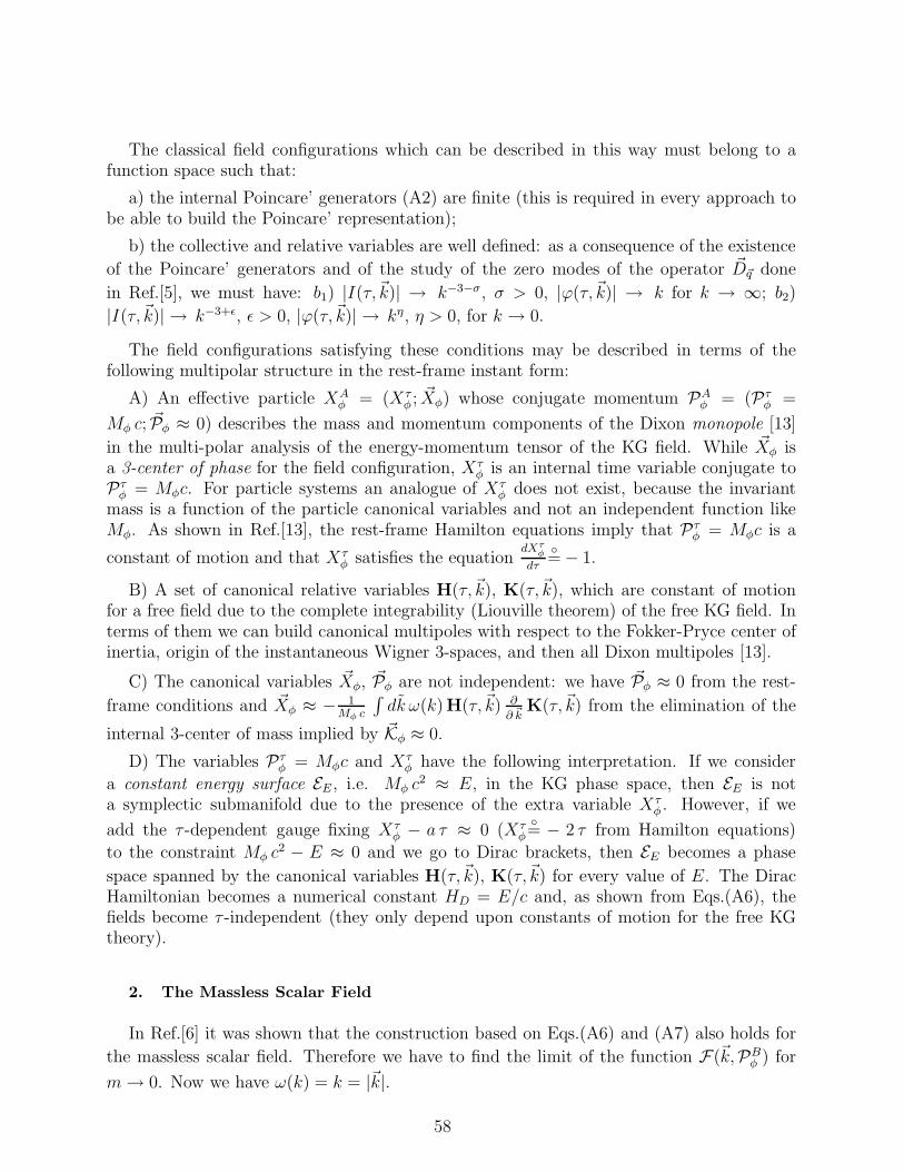
The classical field configurations which can be described in this way must belong to afunction space such that:

a) the internal Poincare’ generators (A2) are finite (this is required in every approach tobe able to build the Poincare’ representation);

b) the collective and relative variables are well defined: as a consequence of the existence

of the Poincare’ generators and of the study of the zero modes of the operator ~D~q done

in Ref.[5], we must have: b1) |I(τ,~k)| → k−3−σ, σ > 0, |ϕ(τ,~k)| → k for k → ∞; b2)

|I(τ,~k)| → k−3+ǫ, ǫ > 0, |ϕ(τ,~k)| → kη, η > 0, for k → 0.

The field configurations satisfying these conditions may be described in terms of thefollowing multipolar structure in the rest-frame instant form:

A) An effective particle XAφ = (Xτ

φ ; ~Xφ) whose conjugate momentum PAφ = (Pτ

φ =

Mφ c; ~Pφ ≈ 0) describes the mass and momentum components of the Dixon monopole [13]

in the multi-polar analysis of the energy-momentum tensor of the KG field. While ~Xφ isa 3-center of phase for the field configuration, Xτ

φ is an internal time variable conjugate toPτ

φ = Mφc. For particle systems an analogue of Xτφ does not exist, because the invariant

mass is a function of the particle canonical variables and not an independent function likeMφ. As shown in Ref.[13], the rest-frame Hamilton equations imply that Pτ

φ = Mφc is a

constant of motion and that Xτφ satisfies the equation

dXτφ

dτ

= − 1.

B) A set of canonical relative variables H(τ,~k), K(τ,~k), which are constant of motionfor a free field due to the complete integrability (Liouville theorem) of the free KG field. Interms of them we can build canonical multipoles with respect to the Fokker-Pryce center ofinertia, origin of the instantaneous Wigner 3-spaces, and then all Dixon multipoles [13].

C) The canonical variables ~Xφ, ~Pφ are not independent: we have ~Pφ ≈ 0 from the rest-

frame conditions and ~Xφ ≈ − 1Mφ c

∫dk ω(k)H(τ,~k) ∂

∂ ~kK(τ,~k) from the elimination of the

internal 3-center of mass implied by ~Kφ ≈ 0.

D) The variables Pτφ = Mφc and Xτ

φ have the following interpretation. If we consider

a constant energy surface EE , i.e. Mφ c2 ≈ E, in the KG phase space, then EE is nota symplectic submanifold due to the presence of the extra variable Xτ

φ . However, if we

add the τ -dependent gauge fixing Xτφ − a τ ≈ 0 (Xτ

φ= − 2 τ from Hamilton equations)

to the constraint Mφ c2 − E ≈ 0 and we go to Dirac brackets, then EE becomes a phase

space spanned by the canonical variables H(τ,~k), K(τ,~k) for every value of E. The DiracHamiltonian becomes a numerical constant HD = E/c and, as shown from Eqs.(A6), thefields become τ -independent (they only depend upon constants of motion for the free KGtheory).

2. The Massless Scalar Field

In Ref.[6] it was shown that the construction based on Eqs.(A6) and (A7) also holds for

the massless scalar field. Therefore we have to find the limit of the function F(~k,PBφ ) for

m → 0. Now we have ω(k) = k = |~k|.

58

By using the definition of the delta function in the form δ(x) = limǫ→0

(1√π ǫ

e−x2/ǫ)

with ǫ = m2 c2/4π → 0, we get that the functions F τ(k) and F (k) of Eqs.(A5) become thefollowing distribution in the massless limit

F τ (k) =8 π2

k3δ(k), F (k) = −24 π2

k3δ(k). (A11)

It can be checked that the conditions contained in Eqs.(A5) are still satisfied since δ(k)is an even function of k and we have

∫dk ω2(k) F τ (k) = 2

∫ ∞

0

dk δ(k) =

∫ ∞

−∞dk δ(k) = 1,

∫dk kr ks F (k) = −2 δrs

∫ ∞

0

dk δ(k) = −δrs

∫ ∞

−∞dk δ(k) = −δrs. (A12)

The collective variables (A7) are now well defined for the field configurations whose phase

variables behave as ϕ(τ,~k) →k→0 k and have the form

Xτφ =

1

2π

∫d3k

k3δ(k) ϕ(τ,~k),

~Xφ =3

2π

∫d3k

k3~k δ(k) ϕ(τ,~k). (A13)

As shown in Ref.[6] the relative canonical variables, having zero Poisson brackets with

the collective ones, are again given by Eqs.(A9), but now ω(k) = k and G(~k, ~q) is the Green

function of the operator D~q = 3 − 2 ~q · ~∂~q − (~q · ~∂~q)2 28.

Also Eqs.(A10) for the reconstruction of the massless KG fields hold.

Now, the field configurations having well defined collective and relative canonical variablesare restricted by the requirement of the existence of the Poincare’ generators. This requires

[6]: i) |I(τ,~k)| → k−3−δ, δ > 0, and |ϕ(τ,~k)| → k for k → ∞; ii) |I(τ,~k)| → k−2+ǫ,

ǫ > 0, and |ϕ(τ,~k)| → kα, α > −δ for k → 0. However an extra infinite set of integral

restrictions comes from the study of the zero modes wlm(~k) of the operator ~D~q done in

Ref.[6]. If we define the quantities Plm =∫

dk wlm(~k) I(τ,~k), then the restrictions are

Plm ≡∫

dk wlm(~k)F(~k,PBφ ) for l ≥ 2 (the Plm with l > 2 are called super-translations,

being connected with the generators of the algebra of BMS group studied in this frameworkin Ref.[15]).

28 Like in the massive case this operator is scalar, formally self-adjoint with respect the Lorentz invariant

measure for the massless case and has kA = (|~k|;~k) as null eigenvectors.

59

APPENDIX B: RELATIVISTIC LAGRANGIANS FOR THE ELECTRIC

DIPOLE APPROXIMATION

1. The Standard Electric Dipole Representation with Grassmann-valued Electric

Charges

Let us revisit the standard electric dipole representation starting from the Hamiltonian(7.1) with Grassmann-valued charges. we go to the collective and relative variables (2.3) and

we make the dipole approximation (6.2) (i.e. we neglect terms of order O((~ρ12 · ∂

∂ ~η12)2 ~A⊥

)),

we get from the Hamilton equations (µ = m1 m2/m, a = d adτ

, τ = ct,∫

dτ L(τ) =∫

dt L(t))

~κ12(τ) = mc ~η12(τ) +Q

c

(~ρ12(τ) · ∂

∂ ~η12

)~A⊥(τ, ~η12(τ)) +

+Qc

m2 − m1

m

(~ρ12(τ) · ∂

∂ ~η12

)~A⊥(τ, ~η12(τ)),

~π12(τ) = µc ~ρ12(τ) +Q

c

[~A⊥(τ, ~η12(τ)) +

m2 − m1

m

(~ρ12(τ) · ∂

∂ ~η12

)~A⊥(τ, ~η12(τ))

]+

+Qc

[m2 − m1

m~A⊥(τ, ~η12(τ)) +

m21 + m2

2

m2

(~ρ12(τ) · ∂

∂ ~η12

)~A⊥(τ, ~η12(τ))

], (B1)

where the notation of Eq.(6.1) has been used.

Then by means of the inverse Legendre transformation we get the Lagrangian

L =mc

2~η

2

12(τ) +µc

2~ρ

2

12(τ) +

+(Q

c+

Qc

m2 − m1

m

)~η12(τ) ·

(~ρ12(τ) · ∂

∂ ~η12

)~A⊥(τ, ~η12(τ)) +

+2Qc

~η12(τ) · ~A⊥(τ, ~η12(τ)) +(Q

c+

Qc

m2 − m1

m

)~ρ12(τ) · ~A⊥(τ, ~η12(τ)) +

+(Q

c

m2 − m1

m+

Qc

m21 + m2

2

m2,)

~ρ12(τ) ·(~ρ12(τ) · ∂

∂ ~η12

)~A⊥(τ, ~η12(τ)). (B2)

Let us write L = L1 + dSdτ

with the following function S

S =m2 Q1 − m1 Q2

2 m c~ρ12(τ) · ~A⊥(τ, ~η12(τ)) +

+m2

2 Q1 + m21 Q2

2m2~ρ12(τ) ·

(~ρ12(τ) · ∂

∂ ~η12

)~A⊥(τ, ~η12(τ)) =

=Q

c

[~ρ12(τ) · ~A⊥(τ, ~η12(τ)) +

m2 − m1

2m~ρ12(τ) ·

(~ρ12(τ) · ∂

∂ ~η12

)~A⊥(τ, ~η12(τ))

]+

+Qc

[m2 − m1

m~ρ12(τ) · ~A⊥(τ, ~η12(τ)) +

m21 + m2

2

2m2~ρ12(τ) ·

(~ρ12(τ) · ∂

∂ ~η12

)~A⊥(τ, ~η12(τ))

]

→Q≈0Q

c~ρ12(τ) ·

[~A⊥(τ, ~η12(τ)) +

m2 − m1

2m

(~ρ12(τ) · ∂

∂ ~η12

)~A⊥(τ, ~η12(τ))

], (B3)

60

where we used the notation of Eq.(6.1). For neutral systems, Q ≈ 0, S = So + O((~ρ12 ·

∂∂ ~η12

) ~A⊥

)is the extension to the next order of the classical counterpart So of the generator

of the Gøppert-Mayer unitary transformation.

If we use d ~A⊥(τ,~η12(τ))dτ

= −~π⊥(τ, ~η12(τ)) +(~η12(τ) · ∂

∂ ~η12

)~A⊥(τ, ~η12(τ)), L1 takes the fol-

lowing form

L1 =mc

2~η

2

12(τ) +µc

2~ρ

2

12(τ) +2Qc

~η12(τ) · ~A⊥(τ, ~η12(τ)) +

+(Q

c+

Qc

m2 − m1

m

) [~ρ12(τ) · ~π⊥(τ, ~η12(τ)) − ~η12(τ) ·

(~ρ12(τ) × ~B(τ, ~η12(τ))

)]+

+(Q

c

m2 − m1

2m+

Qc

m21 + m2

2

2m2

) [~ρ12(τ) ·

(~ρ12(τ) · ∂

∂ ~η12

)~π⊥(τ, ~η12(τ)) −

− ~ρ12(τ) ·(~ρ12(τ) × ~B(τ, ~η12(τ))

)]. (B4)

We have used ~B(τ, ~η12(τ)) = − ∂∂ ~η12

× ~A⊥(τ, ~η12(τ)), ~ρ12(τ) × ~B(τ, ~η12(τ)) =(~ρ12(τ) ·

∂∂ ~η12

)~A⊥(τ, ~η12(τ)) − ∂

∂ ~η12

(~ρ12(τ) · ~A⊥(τ, ~η12(τ))

). The new momenta are

~κ12(τ) = m c ~η12(τ) +2Qc

~A⊥(τ, ~η12(τ)) −(Q

c+

Qc

m2 − m1

m

)~ρ12(τ) × ~B(τ, ~η12(τ)),

~π12(τ) = µ c ~ρ12(τ) −(Q

c

m2 − m1

2m+

Qc

m21 + m2

2

2m2

)~ρ12(τ) × ~B(τ, ~η12(τ)). (B5)

Then by Legendre transformation we get the Hamiltonian of the electric dipole represen-tation in the dipole approximation

H1 =~κ

212(τ)

2m c+

~π212(τ)

2µ c−

(Q

c+

Qc

m2 − m1

m

)~ρ12(τ) · ~π⊥(τ, ~η12(τ)) −

−(Q

c

m2 − m1

2m+

Qc

m21 + m2

2

2m2

)~ρ12(τ) ·

(~ρ12(τ) · ∂

∂ ~η12

)~π⊥(τ, ~η12(τ)) +

+1

mc

(Q

c+

Qc

m2 − m1

m

)~κ12(τ) ·

(~ρ12(τ) × ~B(τ, ~η12(τ))

)+

+1

µ c

(Q

c

m2 − m1

2m+

Qc

m21 + m2

2

2m2

)~π12(τ) ·

(~ρ12(τ) × ~B(τ, ~η12(τ))

)−

− Q1 Q23 µ

4m2 c2

(~ρ12(τ) × ~B(τ, ~η12(τ))

)2

−

− 2Qmc2

[~κ12(τ) · ~A⊥(τ, ~η12(τ)) +

(Q + Q m2 − m1

m

)~A⊥(τ, ~η12(τ)) ·

(~ρ12(τ) × ~B(τ, ~η12(τ))

)]+

+4Q2

2 m c3~A2⊥(τ, ~η12(τ)). (B6)

For 2Q = Q1 + Q2 ≈ 0, e = Q1, we get the Røntgen Hamiltonian (7.2) of the electricdipole representation, given in Eq.(14.37) of Ref.[7].

61

2. A Lagrangian for the Internal Motion of the Particles with an External Electro-

Magnetic Field

Let us now follow the method of Appendix L of Ref.[7] of determining the Lagrangianfrom the Hamiltonian by considering the electro-magnetic field as an external field.

We begin with the internal energy 1cE(int) = Pτ

(int) = Mc of Eqs.(4.1) and we do theinverse Legendre transformation on the particle variables to find an effective Lagrangianfor the particles. After the dipole approximation and by using e = Q1 ≈ −Q2, a term inthe resulting Lagrangian will be a total time derivative identifying the generating functionS. Then we will do the Legendre transformation of the Lagrangian without the total timederivative. The semi-relativistic limit of the resulting Hamiltonian turns out to be theRøntgen Hamiltonian (7.2) of Ref.[7].

By ignoring the field energy Eem in Eq.(4.1), the inverse Legendre transformation producesthe Lagrangian

L(τ) = ~κ1 ·d~η1(τ)

dτ+ ~κ2 ·

d~η2(τ)

dτ− M c =

= −m1 c

√

1 −(

d~η1(τ)

dτ

)2

− m2 c

√

1 −(

d~η2(τ)

dτ

)2

− Q1 Q2

4π c |~η1(τ) − ~η2(τ)| +

+Q1

c~A⊥(τ, ~η1(τ)) · d~η1

dτ+

Q2

c~A⊥(τ, ~η2(τ)) · d~η2

dτ. (B7)

Switching to the center of mass and relative variables of Eqs.(2.3) (here we put ~η = ~η12

and ~ρ = ~ρ12) we obtain

L(τ) = −m1 c

√

1 −(

d~η(τ)

dτ+

m2

m

d~ρ(τ)

dτ

)2

− m2 c

√

1 −(

d~η(τ)

dτ− m1

m

d~ρ(τ)

dτ

)2

−

− Q1 Q2

4π c |~ρ(τ)| +

+Q1

c

(~A⊥(τ, ~η(τ)) +

m2

m

∂

∂ ~η~ρ(τ) · ~A⊥(τ, ~η(τ))

)·(

d~η(τ)

dτ+

m2

m

d~ρ(τ)

dτ

)+

+Q2

c( ~A⊥(τ, ~η(τ)) − m1

m

∂

∂~η~ρ(τ) · ~A⊥(τ, ~η(τ))) ·

(d~η(τ)

dτ− m1

m

d~ρ(τ)

dτ

), (B8)

in which we have expanded the vector potentials about ~η by using the dipole approximation.By using the notation Q = 1

2(Q1 −Q2), Q = 1

2(Q1 + Q2), of Eq.(6.1) after some algebra we

find 29

29 Note that we divided the d~ρ(τ)dτ

· ∂∂ ~η

(~ρ(τ) · ~A⊥(τ, ~η(τ))

)term into separate and equal parts following the

treatment of Ref.[7]: this will produce the correct 12 factors.

62

L(τ) = −m1 c

√

1 −(

d~η(τ)

dτ+

m2

m

d~ρ(τ)

dτ

)2

− m2 c

√

1 −(

d~η(τ)

dτ− m1

m

d~ρ(τ)

dτ

)2

+

+Q1 Q2

4π c |~ρ(τ)| +Q

c

(~ρ(τ) · ~π⊥(τ, ~η(τ)) +

∆m

2m~ρ(τ) · ∂

∂ ~η

(~ρ · ~π⊥(τ, ~η(τ))

)−

− d~η(τ)

dτ·[ ∂

∂ ~η

(~ρ · ~A⊥(τ, ~η(τ))

)− ~ρ(τ) · ∂

∂ ~η~A⊥(τ, ~η(τ))

]+

+∆m

2m

d~ρ(τ)

dτ·[~ρ(τ) · ∂

∂ ~η~A⊥(τ, ~η(τ)) − ∂

∂ ~η

(~ρ(τ) · ~A⊥(τ, ~η(τ))

)])+

+Qc

(~η(τ) · ~π⊥(τ, ~η(τ)) +

∆m

m~ρ(τ) · ~π⊥(τ, ~η(τ)) +

+m2 − 2µm

2m2~ρ(τ) ·

(~ρ(τ) · ∂

∂ ~η~π⊥(τ, ~η)

)+

+m2 − 2µm

2m2

d~ρ(τ)

dτ·[~ρ(τ) · ∂

∂ ~η~A⊥(τ, ~η(τ)) − ∂

∂ ~η

(~ρ(τ) · ~A⊥(τ, ~η(τ))

)]−

− ~η(τ) ·(d~η(τ)

dτ· ∂

∂ ~η

)~A⊥(τ, ~η(τ)) +

+∆m

m

d~η(τ)

dτ·[~ρ(τ) · ∂

∂ ~η~A⊥(τ, ~η(τ)) − ∂

∂ ~η

(~ρ(τ) · ~A⊥(τ, ~η(τ))

)]−

− ~η(τ) ·(d~η(τ)

dτ· ∂

∂ ~η

)~A⊥(τ, ~η(τ))

)+

dS

dτ=

def= L1(τ) +

dS

dτ. (B9)

in which we have ignored the second order spatial gradient terms of the vector potential(dipole approximation) and we have put m = m2 − m1, µ = m1 m2

m.

The total time derivative terms, not contributing to the equations of motion, identify thegenerating function S:

S =Q

c

[~ρ(τ) · ~A⊥(τ, ~η(τ)) +

∆m

2m~ρ(τ) ·

(~ρ(τ) · ∂

∂ ~η~A⊥(τ, ~η(τ))

)]+

+Qc

[~η(τ) · ~A⊥(τ, ~η(τ)) +

∆m

m~ρ(τ) · ~A⊥(τ, ~η(τ)) +

+m2 − 2µm

2m2~ρ(τ) ·

(~ρ(τ) · ∂

∂ ~η~A⊥(τ, ~η(τ))

)]. (B10)

Since we are in the radiation gauge we have ~E⊥(τ, ~η(τ)) = −∂ ~A⊥(τ,~η(τ))∂ τ

. Then by using

63

~ρ × ~B =∂

∂ ~η

(~ρ · ~A⊥(τ, ~η)

)− ~ρ · ∂

∂ ~η~A⊥(τ, ~η),

~η ·(d~η

dτ· ~∇

)~A⊥(τ, ~η) =

d~η

dτ·( ∂

∂ ~η

(~η · ~A⊥(τ, ~η)

)− ~A⊥(τ, ~η)

),

~η × ~B = ~A⊥(τ, ~η) − ∂

∂ ~η~η · ~A⊥(τ, ~η) − ~η · ∂

∂ ~η~A⊥(τ, ~η),

d~η

dτ· ~η × ~B = −~η ·

(d~η

dτ· ∂

∂ ~η

)~A⊥(τ, ~η) − d~η

dτ·(~η · ∂

∂ ~η

)~A⊥(τ, ~η)),

(B11)

we obtain

L1(τ) = −m1 c

√

1 −(

d~η(τ)

dτ+

m2

m

d~ρ(τ)

dτ

)2

− m2 c

√

1 −(

d~η(τ)

dτ− m1

m

d~ρ(τ)

dτ

)2

−

− Q1Q2

4π c |~ρ(τ)| +Q

c

(~ρ(τ)·~π⊥(τ, ~η(τ)) +

∆m

2m~ρ(τ) ·

(~ρ(τ) · ∂

∂ ~η~π⊥(τ, ~η(τ))

)−

− d~η(τ)

dτ· ~ρ(τ) × ~B(τ, ~η(τ)) − ∆m

2m

d~ρ(τ)

dτ· ~ρ(τ) × ~B(τ, ~η(τ))

)+

+Qc

(∆m

m~ρ(τ)·~π⊥(τ, ~η(τ)) +

m2 − 2µm

2m2~ρ(τ) ·

(~ρ(τ) · ∂

∂ ~η~π⊥(τ, ~η(τ))

)−

− m2 − 2µm

2m2

d~ρ(τ)

dτ· ~ρ(τ) × ~B(τ, ~η(τ)) −

− ∆m

m

d~η(τ)

dτ· ~ρ(τ) × ~B(τ, ~η(τ)) +

d~η(τ)

dτ· ~A⊥(τ, ~η(τ))

). (B12)

In the case e = Q ≈ Q1 ≈ −Q2, Q ≈ 0, this becomes

L1(τ) = −m1 c

√

1 −(

d~η(τ)

dτ+

m2

m

d~ρ(τ)

dτ

)2

− m2 c

√

1 −(

d~η(τ)

dτ− m1

m

d~ρ(τ)

dτ

)2

+

+e2

4π c |~ρ(τ)| +e

c~ρ(τ) · ~π⊥(τ, ~η(τ)) +

e

c

∆m

2m~ρ(τ) ·

(~ρ(τ) · ∂

∂ ~η~π⊥(τ, ~η(τ))

)−

− e

c

d~η(τ)

dτ· ~ρ(τ) × ~B(τ, ~η(τ)) − e

c

∆m

2m

d~ρ(τ)

dτ· ~ρ(τ) × ~B(τ, ~η(τ)). (B13)

and the generating function S reduces to

S =e

c~ρ(τ) ·

[~A⊥(τ, ~η(τ))+

∆m

2m

(~ρ(τ)· ∂

∂ ~η

)~A⊥(τ, ~η(τ)))

]. (B14)

In order to obtain the Hamiltonian from Eq.(B12) we revert from the composite variablesback to the constituent variables, which mean that we need to rewrite L in terms of theindividual velocities using ~η = ~η12 = m1 ~η1+m2 ~η2

m, ~ρ = ~ρ12 = ~η1 − ~η2.

64

We obtain

L1(τ) = −m1 c

√

1 −(

d~η1(τ)

dτ

)2

− m2 c

√

1 −(

d~η2(τ)

dτ

)2

+

+d~η1(τ)

dτ· ~A1(τ, ~η(τ)) +

d~η2(τ)

dτ· ~A2(τ, ~η(τ)) −

− Q1Q2

4π c |~ρ(τ)| +Q

c~ρ(τ)·~π⊥(τ, ~η(τ)) +

Q

c

∆m

2m~ρ(τ) ·

(~ρ(τ) · ∂

∂ ~η~π⊥(τ, ~η(τ))

)+

+Qc

∆m

m~ρ(τ)·~π⊥(τ, ~η(τ)) +

Qc

m2 − 2µm

2m2~ρ(τ) ·

(~ρ(τ) · ∂

∂ ~η~π⊥(τ, ~η(τ))

), (B15)

where

~Ai(τ) =Qmi

cm~A⊥(τ, ~η(τ)) −

−(Q mi

mc+ (−)i+1 Q

c

∆m

2m+

Qc

m2 − 2µ m

2m2+

Qc

∆m mi

m2

)~ρ(τ) × ~B(τ, ~η(τ)).

(B16)

By evaluating the new momenta

~κ′

i(τ) =∂L1(τ)

∂ d~ηi(τ)dτ

=mi c

d~ηi(τ)dτ√

1 −(

d~ηi(τ)dτ

)2+ ~Ai(τ). (B17)

we obtain after some manipulations the Hamiltonian

H1 = ~κ′

1(τ) · d~η1(τ)

dτ+ ~κ

′

2(τ) · d~η2(τ)

dτ− L1 =

=

√m2

1 c2 + (~κ′

1(τ) − ~A1(τ) )2 +

√m2

2 c2 + (~κ′

2(τ) − ~A2(τ) )2 +

+Q1Q2

4π c |~ρ(τ)| −Q

c~ρ(τ)·~π⊥(τ, ~η(τ)) − Q

c

∆m

2m~ρ(τ) ·

(~ρ(τ) · ∂

∂ ~η

)~π⊥(τ, ~η(τ)) −

− Qc

∆m

m~ρ(τ)·~π⊥(τ, ~η(τ)) − Q

c

m2 − 2µ m

2m2~ρ(τ) ·

(~ρ(τ) · ∂

∂ ~η

)~π⊥(τ, ~η(τ)).

(B18)

This can be brought to desired form using relative variables by substituting for ~κi andexpanding the vector potential from the square root by using the Grassmann property.

Consider first the non-relativistic limit (in which we keep terms of order 1/c). First weuse

√m2

i c2 + (~κ′

i(τ) − ~Ai(τ) )2 =√

m2i c2 + ~κi

′ 2(τ) − ~κ′

i(τ) · ~Ai(τ)√m2

i c2 + ~κi′ 2(τ)

. (B19)

65

Note that we cannot use the Grassmann argument to eliminate the ~A2(τ) terms since

they involve the nonzero Q2 = −2 Q1 Q2 terms even with Q ≈ 0 terms. We shall insteadignore them as being too high an order of 1/c2. So we get

H1 =√

m21 c2 + ~κ1

′ 2(τ) − ~κ′

1(τ) · ~A1(τ)√m2

1 c2 + ~κ1′ 2(τ)

+√

m22 c2 + ~κ2

′ 2(τ) − ~κ′

2(τ) · ~A2(τ)√m2

2 c2 + ~κ2′ 2(τ)

+

+Q1Q2

4π c |~ρ(τ)| −Q

c~ρ(τ) · ~π⊥(τ, ~η(τ)) − Q

c

∆m

2m~ρ(τ) ·

(~ρ(τ) · ∂

∂ ~η

)~π⊥(τ, ~η(τ)) −

− Qc

∆m

m~ρ(τ)·~π⊥(τ, ~η(τ)) − Q

c

m2 − 2µ m

2m2~ρ(τ) ·

(~ρ(τ) · ∂

∂ ~η

)~π⊥(τ, ~η(τ)). (B20)

In terms of the relative and collective variables

H1 =

√m2

1 c2 + (m1

m~κ′(τ) + ~π′(τ))2 − (m1

m~κ

′

(τ) + ~π′

(τ)) · ~A1(τ)√m2

1 c2 + (m1

m~κ′(τ) + ~π′(τ))2

+

+

√m2

2 c2 + (m2

m~κ′(τ) − ~π′(τ))2 − (m2

m~κ

′

(τ) − ~π′

(τ)) · ~A2(τ)√m2

2 c2 + (m2

m~κ′(τ) − ~π′(τ))2

+

+Q1Q2

4π c |~ρ(τ)| −Q

c~ρ(τ)·~π⊥(τ, ~η(τ)) − Q

c

∆m

2m~ρ(τ) ·

(~ρ(τ) · ∂

∂ ~η

)~π⊥(τ, ~η(τ)) −

− Qc

∆m

m~ρ(τ)·~π⊥(τ, ~η(τ)) − Q

c

m2 − 2µ m

2m2~ρ(τ) ·

(~ρ(τ) · ∂

∂ ~η

)~π⊥(τ, ~η(τ)). (B21)

Next, look at the limit as c → ∞ in which

√m2

i c2 + (mi

m~κ′(τ) + (−)i+1 ~π′(τ))2 → mi c +

(mi

m~κ

′

(τ) + (−)i+1 ~π′

(τ))2

2mi c,

1√m2

i c2 + (mi

m~κ′(τ) + (−)i+1 ~π′(τ))2

→ 1

mi c− (mi

m~κ

′

(τ) + (−)i+1 ~π′

(τ))2

2 m3i c3

, (B22)

and we keep only the terms of O(1/c) and lower obtaining

H1 c = m c2 +~κ

′ 2(τ)

2m+

~π′ 2(τ)

2µ− ~κ

′

(τ)

m·(

~A1(τ) + ~A2(τ))− ~π

′

(τ) ·( ~A1(τ)

m1−

~A2(τ)

m2

)+

+Q1 Q2

4π |~ρ(τ)| − Q ~ρ(τ)·~π⊥(τ, ~η(τ)) − Q∆m

2m~ρ(τ) ·

(~ρ(τ) · ∂

∂ ~η

)~π⊥(τ, ~η(τ)) −

− Q ∆m

m~ρ(τ)·~π⊥(τ, ~η(τ)) −Q m2 − 2µ m

2m2~ρ(τ) ·

(~ρ(τ) · ∂

∂ ~η

)~π⊥(τ, ~η(τ)).

(B23)

Now using Eq.(B16) we obtain in the non-relativistic limit

66

H1 c = m c2 +~κ

′ 2(τ)

2m+

~π′ 2(τ)

2µ+

+~κ

′

(τ)

m·[(Q

c+

Qc

∆m

m

)~ρ(τ) × ~B(τ, ~η(τ)) − Q

c~A⊥(τ, ~η(τ))

]+

+(Q

c

∆m

2m µ+

Qc

m2 − 2µ m

2m2µ

)~π

′

(τ) · ~ρ(τ) × ~B(τ, ~η(τ)) +

+Q1 Q2

4π |~ρ(τ)| − Q ~ρ(τ)·~π⊥(τ, ~η(τ)) − Q∆m

2m~ρ(τ) ·

(~ρ(τ) · ∂

∂ ~η

)~π⊥(τ, ~η(τ)) −

− Q ∆m

m~ρ(τ)·~π⊥(τ, ~η(τ)) −Q m2 − 2µ m

2m2~ρ(τ) ·

(~ρ(τ) · ∂

∂ ~η

)~π⊥(τ, ~η(τ)). (B24)

If we use Q ≈ 0, e = Q ≈ Q1 ≈ −Q2, we get

H1 c = m c2 +~κ

′ 2(τ)

2m− e2

4π |~ρ(τ)| +

+~π

′ 2(τ)

2µ+

~κ′

(τ)

m· e

c~ρ(τ) × ~B(τ, ~η(τ)) +

e

c

∆m

2mµ~π

′

(τ) · ~ρ(τ) × ~B(τ, ~η(τ)) −

− e ~ρ(τ)·~π⊥(τ, ~η(τ)) − e∆m

2m~ρ(τ) ·

(~ρ(τ) · ∂

∂ ~η

)~π⊥(τ, ~η(τ)),

(B25)

which agrees with Eq.(L.14) and (14.37) of Ref.[8] with e2 = 0 (one could also find the e2

terms of Eq.(7.2)).

3. A Lagrangian for the Internal Motion of the Particles plus the Electro-Magnetic

Field

Let us consider the isolated system ”charged particles with mutual Coulomb interactionplus the transverse electromagnetic field” inside the instantaneous Wigner 3-spaces. Itsmotion is determined by the Hamiltonian Mc = 1

cE(int) given in Eqs.(4.1) and then restricted

by the rest-frame conditions ~P(int) ≈ 0 and by their gauge fixing ~K(int) ≈ 0. Therefore wecan look for the Lagrangian corresponding to the Hamiltonian Mc.

By using the first half of the Hamilton equations with Hamiltonian Mc

67

d ~ηi(τ))

dτ= ~ηi(τ), Mc =

~κi(τ) − Qi

c~A⊥(τ, ~ηi(τ))√

m2i c2 + (~κi(τ) − Qi

c~A⊥(τ, ~ηi(τ)) )2

,

∂ ~A⊥(τ, ~σ)

∂ τ

= ~A⊥(τ, ~σ), Mc = −~π⊥(τ, ~σ),

⇓

~κi(τ)=

mi cd~ηi

dτ√1 −

(d~ηi

dτ

)2+

Qi

c~A⊥(τ, ~ηi(τ)),

⇒√

m2i c2 + (~κi(τ) − Qi

c~A⊥(τ, ~ηi(τ)) )2

=mi c√

1 − (d~ηi(τ)dτ

)2

, (B26)

the inverse Legendre transformation leads to the following Lagrangian

L(τ) =

∫d3σ

(∑

i

δ3(~σ − ~ηi(τ))[~κi(τ) · d ~ηi(τ)

dτ

]− 1

c

[~π⊥ · ∂ ~A⊥

∂ τ

](τ, ~σ)

)−

− 1

cE(int) =

=

∫d3σ

(∑

i

δ3(~σ − ~ηi(τ))[− mi c

√1 − (

d ~ηi(τ)

dτ)2 −

− Q1 Q2

8π c |~η1(τ) − ~η2(τ)| +Qi

c

d ~ηi(τ)

dτ· ~A⊥(τ, ~σ)

]+

+1

2c

[(∂ ~A⊥∂ τ

)2 − ~B2](τ, ~σ)

)=

=

∫d3σ

(∑

i

δ3(~σ − ~ηi(τ))[− mi c

√1 − (

d ~ηi(τ)

dτ)2 − Q1 Q2

8π c |~η1(τ) − ~η2(τ)| −

− Qi

c~ηi(τ) ·

(∂ ~A⊥(τ, ~σ)

∂ τ+

d ~ηi(τ)

dτ· ∂ ~A⊥(τ, ~σ)

∂ ~σ

) ])+

+1

2c

∫d3σ

[(∂ ~A⊥∂ τ

)2 − ~B2](τ, ~σ) +

d S2(τ)

dτ=

= L1(τ) +d S2(τ)

dτ. (B27)

In the last lines we have redefined the Lagrangian by isolating a total time derivative.This leads to the identification of the following generating function

68

S2 =1

c

∑

i

∫d3σ δ3(~σ − ~ηi(τ)) Qi ~ηi(τ) · ~A⊥(τ, ~σ) =

=1

c

∑

i

Qi ~ηi(τ) · ~A⊥(τ, ~ηi(τ)) =

=Q

c

[~ρ12(τ) · ~A⊥(τ, ~η12(τ) +

+m2 − m1

m~ρ12(τ) ·

(~ρ12(τ) · ∂

∂ ~η12

)~A⊥(τ, ~η12(τ)) +

+ ~η12(τ) ·(~ρ12(τ) · ∂

∂ ~η12

)~A⊥(τ, ~η12(τ))

]+

+Qc

2∑

i=1

~ηi(τ) · ~A⊥(τ, ~ηi(τ)) + O((~ρ12 ·

∂

∂ ~η12)2 ~A⊥

)

→Q≈0Q

c

[~ρ12(τ) · ~A⊥(τ, ~η12(τ)) +

+m2 − m1

m~ρ12(τ) ·

(~ρ12(τ) · ∂

∂ ~η12

)~A⊥(τ, ~η12(τ)) +

+ ~η12(τ) ·(~ρ12(τ) · ∂

∂ ~η12

)~A⊥(τ, ~η12(τ))

]+ O

((~ρ12 ·

∂

∂ ~η12

)2 ~A⊥

)=

=1

c~d(τ) ·

[~A⊥(τ, ~η12(τ)) +

m2 − m1

m

(~ρ12(τ) · ∂

∂ ~η12

)~A⊥(τ, ~η12(τ))

]+

+Q

c~η12(τ) ·

(~ρ12(τ) · ∂

∂ ~η12

)~A⊥(τ, ~η12(τ)) + O

((~ρ12 ·

∂

∂ ~η12

)2 ~A⊥

). (B28)

In Eq.(B28) we have shown the dipole approximation of S2. It contains an electric dipoleterm similar to the function S of Eqs.(B3) - (7.3) but with m2−m1

2mreplaced by m2−m1

m.

Moreover it contains an extra term connected to the motion of the collective variable ~η12(τ)of the 2-particle system.

69

[1] H.W.Crater and L.Lusanna, The Rest-Frame Darwin Potential from the Lienard-Wiechert

Solution in the Radiation Gauge, Ann.Phys. (N.Y.) 289, 87 (2001).

[2] D.Alba, H.W.Crater and L.Lusanna, Towards Relativistic Atom Physics. I. The Rest-Frame

Instant Form of Dynamics and a Canonical Transformation for a system of Charged Particles

plus the Electro-Magnetic Field (arXiv: 0806.2383).

[3] L.Lusanna, The Chrono-Geometrical Structure of Special and General Relativity: A Re-

Visitation of Canonical Geometrodynamics, lectures at 42nd Karpacz Winter School of Theo-

retical Physics: Current Mathematical Topics in Gravitation and Cosmology, Ladek, Poland,

6-11 Feb 2006, Int.J.Geom.Methods in Mod.Phys. 4, 79 (2007). (gr-qc/0604120).

[4] D.Alba, H.W.Crater and L.Lusanna, Hamiltonian Relativistic Two-Body Problem: Center of

Mass and Orbit Reconstruction, J.Phys. A40, 9585 (2007) (gr-qc/0610200).

[5] G.Longhi and M.Materassi, Collective and Relative Variables for a Classical Real Klein-

Gordon Field, Int.J.Mod.Phys. A14, 3387 (1999) (hep-th/9809024).

[6] L.Assenza and G.Longhi, Collective and Relative Variables for Massless Fields,

Int.J.Mod.Phys. A15, 4575-4601 (2000).

[7] W.P.Schleich, Quantum Optics in Phase Space (Wiley-VCH, Berlin, 2001).

[8] C.Cohen-Tannoudji, J. Dupont-Roc and G.Grynberg, Atom-Photon Interactions. Basic Pro-

cesses and Applications (Wiley, New York, 1992).

[9] C.Cohen-Tannoudji, J. Dupont-Roc and G.Grynberg, Photons and Atoms. Introduction to

Quantum Electrodynamics (Wiley, New York, 1989).

[10] D.Alba, H.W.Crater and L.Lusanna, Towards Relativistic Atom Physics. III. Clock Synchro-

nization and Quantization, in preparation.

[11] D.Alba, L.Lusanna and M.Pauri, New Directions in Non-Relativistic and Relativistic Ro-

tational and Multipole Kinematics for N-Body and Continuous Systems (2005), in Atomic

and Molecular Clusters: New Research, ed.Y.L.Ping (Nova Science, New York, 2006) (hep-

th/0505005).

D.Alba, L.Lusanna and M.Pauri, Centers of Mass and Rotational Kinematics for the Rela-

tivistic N-Body Problem in the Rest-Frame Instant Form, J.Math.Phys. 43, 1677-1727 (2002)

(hep-th/0102087).

D.Alba, L.Lusanna and M.Pauri, Multipolar Expansions for Closed and Open Systems of Rel-

ativistic Particles, J. Math.Phys. 46, 062505, 1-36 (2004) (hep-th/0402181).

[12] D.Alba, L.Lusanna and M.Pauri, Dynamical Body Frames, Orientation-Shape Variables and

Canonical Spin Bases for the Nonrelativistic N-Body Problem J.Math.Phys. 43, 373 (2002)

(hep-th/0011014).

[13] L.Lusanna and M.Materassi, A Canonical Decomposition in Collective and Relative Variables

of a Klein-Gordon Field in the Rest Frame Wigner Covariant Instant Form, Int.J.Mod.Phys.

A15, 2821-2916 (2000) (hep-th/9904202).

[14] C.J.Borde’, Quantum Theory of Atom-Wave Beam Splitters and Applications to Multidimen-

sional Atomic Gravito-Inertial Sensors, Gen.Rel.Grav. 36, 475 (2004); Atomic Clocks and

Inertial Sensors, Metrologia 39, 435 (2002).

[15] G.Longhi and M.Materassi, A Canonical Realization of the BMS Algebra, J.Math.Phys. 40,

480 (1999) (hep-th/9803128).

[16] D.Alba and L.Lusanna, Quantum Mechanics in Noninertial Frames with a Multitemporal

70

Quantization Scheme: I. Relativistic Particles, Int.J.Mod.Phys. A21, 2781 (2006) (hep-

th/0502194).

[17] J.Larson, Dynamics of the Jaynes-Cummings and Rabi models: Old Wine in New Bottles,

Phys. Scripta 76, 146 (2007).

71