
Electromagnetic compatibility and interference metrology - US ...
Upload
khangminh22Category
view
1download
0
Integrating Rotordynamic and Electromagnetic
Dynamic Models for Flexible-Rotor Electrical
Machines
Karuna Kalita, BE, MTech
GEORGE GREEN LIBRARY OFSCIENCE AND ENGINEERING
Thesis submitted to the University of Nottingham for the degree of
Doctor of Philosophy
March 2007

This thesis is dedicated to my parents, Mrs Parbati Kalita and Late Harendra Chandra
Kalita and my uncle, Late Jogendra Chandra Kalita for their countless sacrifices

Contents
Abstract
Acknowledgement
Nomenclature
List of Figures
List of Tables
1 Introduction
1.1 General. . . . . . . . . . . . . . . . . . . . . . . . . . . . . . . . . . . . . .
1.2 Eccentricity in an electrical machine .
1.3
1.4
Motivation .
Aim of the research. . . . .
2
1.5 Organisation of the thesis .
Literature Review
x
Xl
Xll
XVlll
xxv
1
1
1
3
4
4
9
2.1 Introduction. . . . . . . . . . . . . . . . . . . . . . . . . . . . . . . . . . . . . . . . . . . . 9
2.2 General observations about the origin of UMP and its effect. . . . . . 10
2.3 Airgap permeance. . . . . . . . . . . . . . . . . . . . . . . . . . . . . . . . . . . . . . . 11
2.4 Conformal transformation technique. . . . . . . . . . . . . . . . . . . . . . . . 11
2.5 Analytical methods of calculating UMP. . . . . . . . . . . . . . . . . . . . . . 12
2.6 Numerical methods for the solution of static magnetic fields. . . . . 16
2.7 Integration of electromagnetic model and mechanical model. . . . . . 20
2.8 Numerical methods for the computation of magnetically-oriented
forces .
1
24

2.8.1
2.8.2
2.8.3
Lorentz force .
Virtual work .
Maxwell stress tensor .
25
25
25
2.9 Experimental findings ofUMP. . . . . . . . . . . . . . . . . . . . . . . . . . . . . 28
2.10 Summary of the literature review. . . . . . . . . . . . . . . . . . . . . . . . . . . 29
3 2-D Finite Element Modelling of Electric Machines 35
3.1 Introduction. . . . . . . . . . . . . . . . . . . . . . . . . . . . . . . . . . . . . . . . . . . . 35
3.2 Basic equations of the electromagnetic field. . . . . . . . . . . . . . . . . . . 36
3.3 Finite element formulation. . . . . . . . . . . . . . . . . . . . . . . . . . . . . . . . . 39
3.4
3.5
3.6
3.3.1
3.3.2
3.3.3
3.3.4
Shape functions .
3.3.1.1
3.3.1.2
3.3.1.3
3.3.1.4
4-Noded quadrilateral element. .
8-Noded quadrilateral element. .
3-Noded triangular element. .
6-Noded triangular element. .
The magnetic stiffness matrix .
Conduction modelling .
Calculation of the magnetomotive forces .
3.3.4.1
3.3.4.2
MMF from current carrying coils .
Magnetomotive force of permanent magnets ..
3.3.5 Calculation of magnetic flux density .
Material properties .
Non-linear finite element analysis .
Computer code for finite element analysis of electromagnetic .
3.6.1 Pre-processor .
3.6.2 Solver .
11
40
41
41
41
42
42
45
48
48
48
49
50
50
52
53
54

3.7
3.8
3.9
3.6.3 55
55
Post-processor .
Case studies for static Unbalance Magnetic Pull (UMP) .
3.7.1 Case study I: Unbalanced magnetic pull of an induction
machine. . . . . . . . . . . . . . . . . . . . . . . . . . .. . . . . . .. . . . . 56
3.7.2 Case study II: Unbalanced magnetic pull of a high speed
permanent magnet alternator (PMA) . . . . . . . . . . . . . . . . . 57
3.7.2.1 Reduction of critical speed due to negative
stiffness. . . . . . . . . . . . . . . . . . . . . . . . . . . . . 57
3.7.3 Case study III: Investigation of tooth passing spatial
harmonics (FPF) with non-magnetic and magnetic slot
wedges .
Magnetic Pull (UMP) for overhung machine .
Summary of the chapter. .
59
60
60
83
83
85
88
4 Co-ordinate Transformations Used in the Magnetic FEA
4.1
4.2
4.3
Introduction. . . . . . . . . . .
General principles of the coordinate transformations .
Transformations of the stator currents .
4.3.1 Transformation of the full set of nodal currents in the
stator to the nodal currents corresponds to the conducting
regions in the stator (Stage I) . . . . . . . . . . . . . . . . . . . . . . 89
4.3.2 Transformation of the nodal currents corresponds to the
conducting regions to the coil side currents in the stator
(Stage II) . . . . . . . . . . . . . . . . . . . . . . . . . . . . . . . . . . . . . . 90
4.3.3 Transformation of the coil side currents to the full coil
currents in the stator (Stage III) . . . . . . . . . . . . . . . . . . . . . 92
4.3.4 Transformation of the full coil currents to the coil group
currents in the stator (Stage IV) .
Transformation of the coil group currents to the terminal
currents (Stage V) .
Transformation of the coil group currents according to
the bridge windings . 95
93
4.3.5
94
4.3.6
111

4.4 Transformations of the rotor bar currents ..................... 974.4.1 Transformation of the full set of nodal currents in the
rotor to the nodal currents corresponds to the conducting
regions (Stage I) ................................ 984.4.2 Transformation of the nodal currents corresponds to the
conducting regions in the rotor to the set of currents
based on the "modes" of conduction (Stage II) ......... 994.4.3 Transformation of the set of currents based on the
"modes" of conduction to the set of nodal currents from
the Fourier transform (stage III) .................... 1024.4.4 Transformation of the set of nodal currents from the
Fourier transform (stage IV) ....................... 1034.5 Transformations of the magnetic potentials. . . . . . . . . . . . . . . . . ... 103
4.5.1 Transformation of the set of nodal potentials in the stator
to apply that tangential-flux conditions ............... 1044.5.2 Transformation of the set of nodal potentials of a hollow
rotor to apply the equal-flux conditions ............... 1054.6 Conclusions ............................................ 105
5 Modelling of Electro-Magneto-Mechanical Devices 116
5.1 Introduction ............................................ 1165.2 Calculation of resistance matrix from finite element method ...... 1175.3 Resistance of the end-windings ............................. 1185.4 Coupled electromagnetic model for an EMM device with
changeable geometry .................................... 1215.5 Modelling of an induction machine .......................... 1255.6 Conclusions ............................................ 128
6 Time-marching Simulations of Rotating Electric Machinery 131
6.1 Introduction ............................................ 131
6.2 Accommodating movement in rotating electric machine modelling. 132
iv

6.3
6.4
6.5
6.6
6.7
Established approaches for accommodating movement in
FE models .
6.2.2 Approaches used in this thesis for accommodating
6.2.1
132
Some general features of machine modelling .
movement. . . . . . . . . . . . . . . . . . . . . . . . . . . . . . . . . . . . . . 134
6.3.1 Revisit of the electro-magneto-mechanical model. .
135
135
6.3.2 Definition and calculation of marginal inductance and its
derivative. . . . . . . . . . . . . . . . . . . . . . . . . . . . . . . . . . . . . 137
Marginal inductance and its rate of change from non-
linear finite element analysis with geometry change .....
Marginal inductance and its rate of change from linear
finite element analysis with geometry change. . . . . . . . . . 151
Airgap stitching method .
Marginal inductance and its rate of change using airgap
stitching method from non-linear FEA .
6.4.2 Marginal inductance and its rate of change using airgap
stitching method from linear FEA. .
The central circle (CC) method .
6.4.1
6.5.1
6.5.2
6.5.3
6.5.4
Formulation of the rotor .
Formulation of the stator .
Coupling the rotor and stator models .
6.5.5
Case studies .
Conclusions .
7 Methods of Calculating Steady State Solutions for Induction
Machines
7.1
7.2
7.3
Introduction .
Available approaches to calculate steady state solution .
Central circle method with non-linear model reduction .
7.3.1 Formulation for the rotor .
v
139
139
140
144
145
147
149
150
153
155
162
162
163
164
165

7.3.2
7.3.3
Formulation for the stator .
Coupling the rotor and stator models and accounting for
the non-linearity .
7.3.3.1 Method I of accounting for non-linearity .
7.3.3.2
7.3.3.3
Method I of accounting for non-linearity .....
The method of calculation of the nonlinear
167
170
172
174
175
coefficients of the power series .
7.4 Case studies. . . . . . . . . . . . . . . . . . . . . . . . . . . . . . . . . . . . . . . . . . . . 175
Case study I: Sinusoidal voltage with lower level of
saturation .
Case study II: Sinusoidal voltage with higher level of
saturation. . . . . . . . . . . . . . . . . . . . . . .
Conclusions .
7.4.1
7.4.2
7.5
8 Unified Electromagnetic Dynamic and Rotordynamics Model
177
177
178
184
8.1 Introduction. . . . . . . . . . . . . . . . . . . . . . . . . . . . . . . . . . . . . . . . . . . . 184
8.2 Electro-magneto-mechanical model. . . . . . . . . . . . . . . . . . . . . . . . . 186
8.3 Mechanical model. . . . . . . . . . . . . . . . . . . . . . . . . . . . . . . . . . . . . . . 187
8.4 Coupled linearised modeL. . . . . . . . . . . . . . . . . . . . . . . . . . . . . . . . 189
8.5 Reference electromagnetic solution. . . . . . . . . . . . . . . . . . . . . . . . . . 192
8.6 The Time period of an electrical machine. . . . . . . . . . . . . . . . . . . . . 193
8.7 Case study of the coupled electrical and mechanics dynamics of an
induction machine. . . . . . . . . . . . . . . . . . . . . . . . . . . . . . . . . . . . . . . 194
8.7.1
8.7.2
8.7.3
8.7.4
8.7.5
Finite element model of the flexible rotor .
Equalising currents for an eccentric rotor .
Minimum time period of the machine .
Preparing the state transition matrix for the coupled
model. .
Stability of the system .
VI
195
195
196
196
197

8.8
8.7.6 Energy transfer while closing the bridge .
Conclusions .
197
198
9 Method of Reducing Unbalanced Magnetic Pull 208
9.1 Introduction. . . . . . . . . . . . . . . . . . . . . . . . . . . . . . . . . . . . . . . . . . . . 208
9.2 Reduction of UMP in an induction machine using bridge windings. 209
9.3 Conclusions .
10 Experimental Validation
210
212
10.1 Introduction... . . . . . . . . . . . . . . . . . . . . . . . . . . . . . . . . . . . . . . . . . 212
10.2 Design of the test rig. . . . . . . . . . . . . . . . . . . . . . . . . . . . . . . . . . . . . 213
10.2.1 Motor electrical design. . . . . . . . . . . . . . . . . . . . . . . . . . . . 213
10.2.1.1
10.2.1.2
10.2.1.3
Winding scheme .
Full pitch and fractional pitch .
Number of turns in each coil. .
213
213
214
10.2.2 Drive system for the motor and electrical sensors. . . . . . . 215
10.2.2.1 Drive system for the motor. . . . . . . . . . . . . . . . 215
10.2.2.2 Current transducers. . . . . . . . . . . . . . . . . . . . . . 216
10.2.2.3 Voltage transducers. . . . . . . . . . . . . . . . . . . . . 216
10.2.3 Mechanical design of the system. . . . . . . . . . . . . . . . . . . . 216
10.2.4 Other transducers. . . . . . . . . . . . . . . . . . . . . . . . . . . . . . . . 217
10.2.5 Data acquisition. . . . . . . . . . . . . . . . . . . . . . . . . . . . . . . . . 218
10.3 Numerical model verification with experimental results. . . . . . . . . . 218
10.3.1
10.3.2
Mechanical model. .
Electrical model. .
10.3.2.1 No-load test. .
219
220
221
10.3.2.2 Locked-rotor test. . . . . . . . . . . . . . . . . . . . . . . 222
vu

10.4 Results for the modified motor. . . . . . . . . . . . . . . . . . . . . . . . . . . . . 222
10.4.1 Bridge currents and voltages. . . . . . . . . . . . . . . . . . . . . . . 223
10.4.2 Reduction ofUMP. . . . . . . . . . . . . . . . . . . . . . . . . . . . . . . 224
10.5 Conclusions...................... . . . . . . . . . . . . . . . . . . . . . . 225
11 Conclusions and Future Work 241
11.1 Conclusions. . . . . . . . . . . . . . . . . . . . . . . . . . . . . . . . . . . . . . . . . . . . 241
11.2 Future work. . . . . . . . . . . . . . . . . . . . . . . . . . . . . . . . . . . . . . . . . . . . 244
11.2.1 Application to other electrical machines. . . . . . . . . . . . . . 244
11.2.2 Three dimensional analysis. . . . . . . . . . . . . . . . . . . . . . . . 244
11.2.3 Detailed study of the approximate method. . . . . . . . . . . . 244
11.2.4 Optimum scaling in the approximate method. . . . . . . . . . 245
11.2.5 Extending the central circle method for accommodating
eccentricity. . . . . . . . . . . . . . . . . . . . . . . . . . . . . . . . . . . . 246
11.2.6 Automatic differentiation of the inductance with respect
to position. . . . . . . . . . . . . . . . . . . . . . . . . . . . . . . . . . . . . 246
11.2.7 Time dependent transformations. . . . . . . . . . . . . . . . . . . . 247
11.2.8 Passive components in the parallel paths. . . . . . . . . . . . . . 248
11.2.9 Inclusion of torsional dynamics in the coupled model. . . 248
11.2.10 Incorporation of the effect of base plate in the
mechanical model. . . . . . . . . . . . . . . . . . . . . . . . . . . . . . . 248
References 249
Appendix A I
Appendix B XIV
viii

Abstract
The magnetic field within electrical machines causes an interaction between the
electrical and mechanical dynamics of the system. In the simplest cases, when the
rotor mean position is central in the stator, the interaction manifests itself mainly as a
negative stiffness between the rotor and the stator. When the rotor mean position is
offset relative to the stator, then components of force arise whose frequency in the
stationary frame is twice the electrical frequency of the supply.
For induction machines in particular, both the electrical system and the mechanical
system may be quite complex dynamically in the sense that over the range of
frequencies of interest, it is necessary to consider a number of degrees of freedom in
both the electrical part of the model and the mechanical part.
This work sets out a structured and formal approach to the preparation of such
models. Each different combination of voltage and slip is examined separately. In
each case, the first step is to compute the steady-state reference solution for machine
currents as a function of time. Then, the electro-magnetic behaviour of the electrical
machine is linearised around that reference solution. The result is a linear time-
dependent model for the electromagnetic behaviour which is then easily coupled with
a linear model for the mechanical dynamics. The mechanical dynamics are usually
stationary. Floquet methods can then be applied to determine whether the system is
stable and the response of the system to mechanical or electrical perturbations can be
computed quickly.
The analysis method is applied to a particular three-phase induction machine which
has parallel paths integrated into its winding structure in the sense that each of the
phases is split into a "Wheatstone-bridge" arrangement following. Currents passing
diametrically through a phase in the vertical direction account for the main torque-
producing components of stator field. Currents passing diametrically through the
phase in the horizontal direction account for transverse forces. The parallel paths can
IX

be switched to open-circuit or closed-circuit without affecting the torque-producing
function of the machine and all of the stator conductors contribute to torque-
production. For a number of combinations of voltage and slip, the machine is stable
irrespective of whether the parallel paths are open-circuit or not but the effective
damping of the machine for synchronous vibration is shown to be much higher with
the parallel paths in closed-circuit.
x

Acknowledgements
I express my profound gratitude to my supervisor, Professor Seamus Garvey, for his
valuable help, advice, encouragement and fruitful thoughts. My special thanks are
also extended to the University of Nottingham for providing me with the financial
support.
I am thankful to all my previous teachers who have helped me at different stages of
my education. Thanks to all my colleagues and researchers who have greatly
contributed to my research, especially Dr. W. K. S. Khoo.
I wish to express my special thanks to my parents for their unwavering support
throughout my life. I would also like to thank Dr. Kamini Arandhara and Mrs.
Gabrielle Arandhara for their help and advice.
Xl

Nomenclature
{}[]A
{A}
{A}
b
{bR}
{bs}
{bJ
{bJ
B
B
Bo
{B}
{B}
Vector symbol
Matrix symbol
Magnetic vector potential which is function of spatial co-ordinates
Magnetic vector potential vector
Magnetic vector potential vector which is function of spatial co-
ordinates
Nodal potential vector of the rotor
Reduced vector of magnetic potentials
Nodal potential vector of the stator
Number of nodes in a single rotor bar
Nodal free MMF vector in the rotor
Nodal free MMF vector in the stator
Free MMF vector
Free MMF vector which is function of spatial co-ordinates
Magnetic flux density
Magnetic flux density which is function of spatial co-ordinates
Remanent flux density which is function of spatial co-ordinates
Magnetic flux density vector
Magnetic flux density vector which is function of spatial co-ordinates
xu

{Bo} Remanent flux density vector which is function of spatial co-ordinates
[D] Damping matrix
ez Unit vector along z-direction
E Electric field strength which is a function of spatial coordinates
{E} Electric field strength vector
{E} Electric field strength vector which is a function of spatial coordinates
{r] External forces
{fE} Electromagnetic force vector
{fM} Mechanical force vector
[F] Internal rotor damping matrix
[G] Gyroscopic matrix
H Field intensity which is function of spatial co-ordinates
{H} Field intensity vector
[H] Sensitivity matrix
{H} Field intensity vector which is function of spatial co-ordinates
iAlev s iB1evand Three levitation currents in the bridge
1· 1· 1· Three terminal currentsAph ? Bph' Cph
ik Nodal currents corresponding to node k
{I} Nodal current vector
{Ie} Eddy currents vector
{IER
} Full vector of currents in the end-ring links
Xlll

10
{Jo}
k
[K]
[Kmar]
[Kmech]
[KR]
[Ks]
I
[L]
m
[M]
N
{N}
p
Equivalent nodal current vector for permanent magnet
Reduced current vector corresponding to the rotor bar
Reduced current vector corresponding to the stator phase currents
Jacobian matrix
Current density
Current density vector
Number of rotor bars
Magnetic stiffness matrix
Marginal magnetic stiffness matrix
Mechanical stiffness matrix
Stiffness matrix of the rotor
Stiffness matrix of the stator
Axial length of the machine
Inductance
Mass
Mass matrix
Shape function
Shape function vector
Pole pairs
Nodal potentials
Total power dissipated over an element
Instantaneous electrical power
XIV

[p] Matrix which dictates how the individual flux quantities in {<t>} arecoupled to the current variables
{q} Displacement vector
[R] Resistance matrix
r Radius of the rotor
[RE] Diagonal matrix of the link resistances for the end-ring
[Rnc] Resistance matrix associated with the nodal currents
[RR ] Resistance matrix associated with the reduced number of rotor bar
currents
[Rs] Resistance related to the stator
s Slip
[S] Selection matrix
t Time
t1 Thickness of the end-ring
[T] Transformation matrix
Tm Mean torque
Tp Time period of the coupled system
u Horizontal position of the rotor centre
[U] Transformation matrix
v Vertical position of the rotor
WI Width of the area associated with a end-ring link
WD Work done by a current distribution
{V} Externally-applied voltages vector
xv

{x} Instantaneous geometry of the system
[Z] State transition matrix
Greek symbols
(l Relaxation factor
11 Local coordinate
8 Angle of tum of the rotor
[8(.,.)] Matrix function
/1 Permeability
/1xx Permeability along x-direction
/1yy Permeability along y-direction
~] Permeability tensor
v Susceptibility, Local coordinate
p Resistivity
o Conductivity
T Time
¢ Phase angle
{<l> } Magnetic flux vector
W Angular frequency
We Critical speed
We Electrical frequency
nmech Constant mechanical speed of the rotor
XVI

n Mean rotational speed
{9\} Residue vector
xvii

List of figures
1.1 An electrical machine. . . . . . . . . . . . . . . . . . . . . . . . . . .. . . . . . . . . . . 7
1.2 A concentric rotor ('0' is the centre of the axis of rotation). . . . . . . . 8
1.3 An eccentric rotor with static eccentricity ('P' is the centre of theaxis of rotation). . . . . . . . . . . . . . . . . . . . . . . . . . . . . . . . . . . . . . . . . . 8
2.1 UMP from static eccentricity. . . . . . . . . . . . . . . . . . . . . . . . . . . . . . . . 31
2.2 UMP from dynamic eccentricity. . . . . . . . . . . . . . . . . . . . . . . . . . . . . 31
2.3 Airgap of an electric machine with an eccentric rotor. . . . . . . . . . . . . 31
2.4 Z-plane. . . . . . . . . . . . . . . . . . . . . . . . . . . . . . . . . . . . . . . . . . . . . . . . . 32
2.5 T-plane. . . . . . . . . . . . . . . . . . . . . . . . . . . . . . . . . . . . . . . . . . . . . . . . . 32
2.6 The radial and tangential components of magnetic flux. density in theairgap (Binns and Dye, 1973). . . . . . . . . . . . . . . . . . . . . . . . . . . . . . . 32
2.7 Numerical field computation methods (Hameyer and Belmans,1999). . . . . . . . . . . . . . . . . . . . . . . . . . . . . . . . . . . . . . . . . . . . . . . . . . . 33
2.8 Fequency response functions at no load condition. In the figure thickline represents the radial and the dashed line represents thetangential components (Tenhunen, 2003). . . . . . . . . . . . . . . . . . . . . . 33
2.9 The normal and tangential components of magnetic flux. density. . . . 34
2.10 The radial strain for different supply voltages: (a) Series pattern ofstator coils, (b) Equalizing pattern of stator coils (Berman, 1993). . 34
3.1 Master element. . . . . . . . . . . . . . . . . . . . . . . . . . . . . . . . . . . . . . . . . . . 61
3.2 Isoparametric element. . . . . . . . . . . . . . . . . . . . . . . . . . . . . . . . . . . . . 61
3.3 Node point ordering ofa 4-noded quadrilateral element. . . . . . . . . . . 61
3.4 Node point ordering of a 8-noded quadrilateral element. . . . . . . . . . . 62
3.5 Node point ordering of a 3-noded triangular element. . . . . . . . . . . . . 62
XVlll

3.6 Node point ordering of a 6-noded triangular element. ............ 63
3.7 B(H) curves for some permanent magnet (Bastos and Sadowski,2003) ................................................... 63
3.8 Magnetisation curve for a permanent magnet. .................. 64
3.9 Magnetization characteristics in B(H)-form of a typical electricalsteel. ................................................... 64
3.10 Schematic representation of solution procedure of non-linear staticelectromagnetic problem ................................... 65
3.11 FE mesh of the induction motor considered for case study I. ....... 66
3.12 Contour of magnetic vector potential when a sinusoidal currentwhen 3-phase current with a peak of 200 Amps (per slot) is applied. 66
3.13 Normal component of flux density in the middle of the airgap when3-phase current with a peak of 200 Amps (per slot) is applied ...... 67
3.14 Tangential component of flux density in the middle of the airgapwhen 3-phase currents with a peak of 200 (per slot) Amps is applied 67
3.15 Normal stress at the middle of the airgap when a sinusoidal currentwhen 3-phase current with a peak of 200 Amps (per slot) is applied. 68
3.16 Shear stress at the middle of the airgap when a sinusoidal currentwhen 3-phase current with a peak of 200 Amps (per slot) is applied. 68
3.17 Horizontal and vertical force versus eccentricity for the inductionmachine considered for Case Study I when 3-phase currents with apeak of200 Amps (per slot) is applied ........................ 69
3.18 Horizontal and vertical forces for 3-phase currents with differentpeaks (per slot) in the stator for the induction motor considered forcase study I. . . . . . . . . . . . . . . .. . ........................... 69
3.19 FE mesh of permanent magnet alternator (PMA) ................ 70
3.20 Contour plot of magnetic vector potentials of the PMA consideringpermanent magnet excitation only ............................ 71
3.21 Normal component of flux density in the middle of the airgap of thePMA ................................................... 71
3.22 Tangential component of flux density in the middle of the airgap ofthe PMA (when the rotor is concentric with the stator) ............ 72
XIX

3.23 Normal stress in the middle of the airgap of the PMA(when the rotor is concentric with the stator). . . . . . . . . . . . . . . . . . . . 72
3.24 Shear stress in the middle of the airgap of the PMA(when the rotor is concentric with the stator). . . . . . . . . . . . . . . . . . . . 73
3.25 Forces on the rotor along x-direction versus eccentricity for thePMA................................................... 73
3.26 True critical speed when negative stiffness due to UMP is alsoconsidered along with mechanical stiffness versus predicted criticalspeed of the PMA. . . . . . . . . . . . . . . . . . . . . . . . . . . . . . . . . . . . . . . . . 74
3.27 Dimension of the slot. . . . . . . . . . . . . . . . . . . . . . . . . . . . . . . . . . . . . . 75
3.28 A FE mesh. . . . . . . . . . . . . . . . . . . . . . . . . . . . . . . . . . . . . . . . . . . . . . 76
3.29 A FE mesh. . . . . . . . . . . . . . . . . . . . . . . . . . . . . . . . . . . . . . . . . . . . . . 76
3.30 Flux contour with non-magnetic slot wedge with current density of15Almm2 . • . . . . • • • •• •. • .• .• • •• • • •• • •• • • • • • • • . . . •. • • . . • • 77
3.31 Flux contour with magnetic slot wedge with current density of 15Almm2.•.•.••••••..••••...•••••...••••••••••••••••.•••. 77
3.32 Normal component of flux d~nsity in the airgap with current densityof 15 Almm for non-magnetic slot wedge. . . . . . . . . . . . . . . . . . . . . 78
3.33 Normal component of flux density in the airgap with current densityof 15 Almm for magnetic slot wedge. . . . . . . . . . . . . . . . . . . . . . . . . 78
3.34 Tangential component of flux density in the airgap with currentdensity of 15 Almm2 for non-magnetic slot wedge. . . . . . . . . . . . . . . 79
3.35 Tangential component of flux density in the airgap with currentdensity of 15 Azmm" for magnetic slot wedge. . . . . . . . . . . . . . . 79
3.36 Normal stress in the airgap with current density of 15 Almm2 fornon-magnetic slot wedge. . . . . . . . . . . . . . . . . . . . . . . . . . . . . . . . . . . 80
3.37 Normal stress in the airgap with current density of 15 Almm2 formagnetic slot wedge. . . . . . . . . . . . . . . . . . . . . . . . . . . . . . . . . . . . . . . 80
3.38 Schematic view of an electrical machine with an overhung rotor. . . . 82
3.39 Equivalent system. . . . . . . . . . . . . . . . . . . . . . . . . . . . . . . . . . . . . . . . 82
4.1 An electric circuit (for illustration purpose only). . . . . . . . . . . . . . . . . 107
xx
4.2 Flow diagram showing the different transformations of statorcurrents ................................................. 108
4.3 Stator of an induction machine showing the winding connection.Red, blue and yellow colours show the three different phases ...... 109
4.4 Winding connection of a 4-pole, 3-phase Induction Motor ......... 109
4.5 Part of the stator core descretised with three 4-noded elements ..... 110
4.6 Stator slot with two sets of coil 1 and 2........................ 110
4.7 One Stator slot shown in Figure (4.6) showing the finite elementnodes when discretized with two elements ..................... 111
4.8 4-pole, 3-phase Induction Motor with a Bridge ConfiguredWindings ............................................... 111
4.9 Rotor of an induction machine with 32 bars .................... 112
4.10 Flow diagram showing the different transformation of rotor ........ 113
4.11 First three modes of conduction of a typical rotor bar ............. 114
4.12 A notional stator of an electrical machine ...................... 115
4.13 A notional rotor of an electrical machine ....................... 115
5.1 Cross section of rotor end-rings .............................. 129
5.2 Cross section of rotor end-rings with seven links (three along thecircumferential and four along the radial direction) ............... 129
5.3 Stator, rotor and airgap of an electric machine .................. 130
6.1 Rotor movement modeling by airgap stitching method ............ 157
6.2 Rotor movement modeling by central circle method .............. 157
6.3 One quarter of an electric machine discretized with 4-nodedquadrilateral and 3-noded triangular finite elements .............. 158
6.4 Rotor and stator with common central circle .................... 158
6.5 Stator currents of an induction machine by airgap stitching methodwhen slip = 10% and supply voltage = 20V ..................... 160
6.6 Rotor currents of an induction machine by airgap stitching methodwhen slip = 10% and supply voltage = 20V ..................... 160
XXI

6.7 Stator currents of an induction machine by central circle methodwhen slip = 10% and supply voltage = 20V. . . . . . . . . . . . . . . . . . . . . 161
6.8 Rotor currents of an induction machine by central circle methodwhen slip = 10% and supply voltage = 20V. . . . . . . . . . . . . . . . . . . . . 161
7.1 A simple electromagnetic device. . . . . . . . . . . . . . . . . . . . . . . . . . . . . 179
7.2 FE Mesh of the model (region A and region B). . . . . . . . . . . . . . . . . . 179
7.3 Contour plot of magnetic potentials. . . . . . . . . . . . . . . . . . . . . . . . . . . 180
7.4 Currents in the region A, t, from linear, approximateI and full non-linear methods for case study I. . . . . . . . . . . . . . . . . . . . . . . . . . . . . . . 180
7.5 Currents in the region B, ib from linear, approximateI and full non-linear methods for case study I. . . . . . . . . . . . . . . . . . . . . . . . . . . . . . . 181
7.6 Currents in the region A, ia from linear, approximate! and full non- 181linear methods for case study II. .
7.7 Currents in the region B, ib from linear, approximateI and full non-linear methods for case study II. . . . . . . . . . . . . . . . . . . . . . . . . . . . . . 182
7.8 Currents in the region A, ia from approximatel, approximatell andfull non-linear methods for case study II. . . . . . . . . . . . . . . . . . . . . . . 182
7.9 Currents in the region B, ib from approximatel, approximatell andfull non-linear methods for case study II. . . . . . . . . . . . . . . . . . . . . . . 183
8.1 Schematic diagram of an induction machine. . . . . . . . . . . . . . . . . . . . 199
8.2 Finite element model of the induction machine. . . . . . . . . . . . . . . . . . 200
8.3 Natural speed versus rotor speed. . . . . . . . . . . . . . . . . . . . . . . . . . . . . 201
8.4 First four modes of the system. . . . . . . . . . . . . . . . . . . . . . . . . . . . . . . 201
8.5 Equalising current per meter of axial length in phase A bridge for aneccentricity of 2% of the airgap and when supply frequency is 25 Hzand slip is 2%. . . . . . . . . . . . . . . . . . . . . . . . . . . . . . . . . . . . . . . . . . . . 202
8.6 Equalising current per meter of axial length in phase B bridge for aneccentricity of2% of the airgap and when supply frequency is 25 Hzand slip is 2%. . . . . . . . . . . . . . . . . . . . . . . . . . . . . . . . . . . . . . . . . . . . 202
8.7 Equalising current per meter of axial length in phase C bridge for aneccentricity of 2% of the airgap and when supply frequency is 25 Hzand slip is 2%. . . . . . . . . . . . . . . . . . . . . . . . . . . . . . . . . . . . . . . . . . . . 203
xxii

8.8
8.9
8.10
8.11
8.12
9.1
9.2
10.1
10.2
10.3
10.4
10.5
10.6
10.7
10.8
10.9a
10.9b
10.10
Equalising current per meter of axial length in phase A bridge for aneccentricity of 10% of the airgap and when supply frequency is 25Hz and slip is 2% .
Equalising current per meter of axial length in phase B bridge for aneccentricity of 10% of the airgap and when supply frequency is 25Hz and slip is 2% .
Equalising current per meter of axial length in phase C bridge for aneccentricity of 10% of the airgap and when supply frequency is 25Hz and slip is 2% .
Energy transfer to the electrical system from the mechanical motiondue to forward whirling .
Energy transfer to the electrical system from the mechanical motiondue to backward whirling .
Stator of an electrical machine showing the winding connection.Red, blue and yellow colours show the three different phases .
4-pole, 3-phase induction motor with a bridge configured windings.
Experimental setup .
MMF harmonics with fractional pitch - ~ of the stator windings ....9
A simply supported beam with a concentrated load .
Test setup of impact hammer excitation experiment. .
Experimental setup showing the stator with the strain gauges .
Output voltage of the strain gauge amplifier when the load is appliedalong x-direction .
Output voltage of the strain gauge amplifier when the load is appliedalong y-direction .
A schematic diagram of the experimental rig (all dimensions are inmm) .
Excitation points on the base of the experimental rig .
Excitation points on the shaft of the experimental rig .
Frequency responses from the strain gauge in dB 01N) for non-rotating shaft .
XXlll
203
204
204
207
207
211
211
226
227
227
228
229
229
230
230
231
231
232

10.11 Mode shape at 1.35 Hz. 'Cyan' and 'red' colours show the un-deflected and deflected rotor respectively. 'Green' and 'blue'colours show the un-deflected and deflected base respectively. . . . . . 233
10.12 Mode shape at 58.61 Hz. 'Cyan' and 'red' colours show the un-deflected and deflected rotor respectively. 'Green' and 'blue'colours show the un-deflected and deflected base respectively. . . . . . 233
10.13 Mode shape at 65.78 Hz. 'Cyan' and 'red' colours show the un-deflected and deflected rotor respectively. 'Green' and 'blue'colours show the un-deflected and deflected base respectively. . . . . . 234
10.14 Mode shape at 72.39 Hz. 'Cyan' and 'red' colours show the un-deflected and deflected rotor respectively. 'Green' and 'blue'colours show the un-deflected and deflected base respectively. . . . . . 234
10.15 Noload supply voltages from numerical model as well experimentswhen supply frequency is 20 Hz. . . . . . . . . . . . . . . . . . . . . . . . . . . . . 235
10.I6 Noload stator currents from numerical model as well experimentswhen supply frequency is 20 Hz. . . . . . . . . . . . . . . . . . . . . . . . . . . . . 235
10.17 Noload supply voltages from numerical model as well experimentswhen supply frequency is 25 Hz. . . . . . . . . . . . . . . . . . . . . . . . . . . . . 236
10.18 Noload stator currents from numerical model as well experimentswhen supply frequency is 25 Hz. . . . . . . . . . . . . . . . . . . . . . . . . . . . . 236
10.19 Supply voltages for locked rotor test from numerical model andexperiments. . . . . . . . . . . . . . . . . . . . . . . . . . . . . . . . . . . . . . . . . . . . . 237
10.20 Stator currents from numerical and experiments for locked rotor test. 237
10.21 Equalising voltages from experiments when supply frequency is 20Hz..................................................... 238
10.22 Equalising currents from experiments when supply frequency is 20Hz. . . . . . . . . . . . . . . .. .. . ... . . . . . . . . . . . . .. . . . .. . .. . . .. . . . . . 238
10.23 Equalising voltages from experiments when supply frequency is 25Hz...................................................... 239
10.24 Equalising currents from experiments when supply frequency is 25Hz..................................................... 239
10.25 Frequency response when the supply frequency is 25 Hz with OPENbridge (blue) and CLOSED bridge (red). . .. . .. .. . . . .. . . . . . . . . . 240
10.26 Rotor centre orbit with OPEN and CLOSED bridge when the supplyfrequency is 25 Hz. . . . . . . . . . . . . . . . . . . . . .. . . . . . . . . . . . . . . . . . . 240
XXIV

List of tables
3.1
3.2
3.3
3.4
6.1
8.1
8.2
8.3
8.4
8.5
8.6
10.1
Parameters of the 2 kW induction motor .
Parameters of the permanent magnet alternator .
Parameters of the 2-pole generator .
Fourier coefficients of normal stress in the airgap for differentlevels of currents in the rotor slot .
Main electromagnetic parameters of the machine .
Main electromagnetic parameters of the machine .
Coefficients of the bearing .
The minimum periods of a machine with parameters given inTable (8.1) for different slips .
Stability chart of the machine at different slips for different voltagelevels .
Time constants with the parallel paths closed for five differentslips in case of forward whirling .
Time constants with the parallel paths closed for five differentslips in case of backward whirling .
MMF harmonics with different slot combinations .
xxv
65
70
75
81
159
199
200
205
205
206
206
226

Chapter One
Introduction
1.1 General
Rotating electrical machines playa very important role in industry. Electric motors
consume something in the order of two-thirds of all electrical power used in industry.
Therefore, the efficiency of these motors is also a major environmental factor.
Besides, there is also a strong industrial demand for reliable and safe operation of
rotating machines (Devanneaux, et al., 2003).
Most of the electrical machines comprise two parts: the cylindrical rotating member
called the rotor and the annular stationary member called the stator. Figure (1.1)
shows an electrical machine showing the stator and the rotor. The rotor has an axial
shaft which is carried on bearings at each end. The rotor core and stator core are both
constructed from a stack of sheet steel laminations. The constructional and certain
other distinguishing features separate electrical machine into different categories.
Among these machines, the induction machine is by far the most common because of
its relatively simple, robust construction and low price.
1.2 Eccentricity in an electrical machine
Eccentricity refers to an offset between the centre of the rotor core and the centre of
the stator core at any given axial position along the motor length. Clearly, eccentricity
can vary along the length. In this thesis, we are concerned only with machines in
which the stator core is rigidly fixed and the rotor core is relatively short and rigid.
Such rotor cores can translate in directions normal to the axis of rotation and they can
also rotate about axes normal to the rotation axis. In this thesis, we restrict attention to
1

pure translation for reasons which are well-founded. These reasons are exposed
further in a chapter about rotordynamic modelling. Eccentricity is described as being
either static or dynamic depending on whether the offset between the core centres is
constant or whether it is moving (usually in an orbit of some description). Static
eccentricity occurs when the axis of the rotor is not being aligned with that of the
stator although it still rotates about its own axis. This can occur for example simply
due to manufacturing tolerances. Excessive static eccentricity can also occur when the
bearings are incorrectly positioned or become worn. Figures (1.2) and (1.3) show
concentric and eccentric rotor respectively. Dynamic eccentricity is caused by the
centre of rotation of the rotor not being aligned with the rotor axis. The usual causes
of dynamic eccentricity are also manufacturing tolerances, wear and incorrect
manufacture. Rotor 'whirl' near critical speed is another source of dynamic
eccentricity and is an important consideration in large, flexible-shaft machine.
One result of eccentricity is that an uneven distribution of electromagnetic field is
produced in the airgap of an electrical machine. These uneven electromagnetic fields
in the air gap gives rise to electromagnetic forces between the rotor and stator and
termed as Unbalance Magnetic Pull (UMP). The net magnetic forces may often be
significant and the direction of these net forces is often such that they tend to pull the
rotor away from the centre position. In other words the magnetic field within every
rotating electrical machine creates a coupling between the eccentricity of the rotor
relative to the stator and the net magnetic force. This "coupling" behaves like a
bearing with very complicated (speed, frequency and load dependent) properties that
is not fully understood. The effect of UMP on the dynamics of a machine is often
equivalent to a strong negative stiffness between rotor and stator. In extreme cases, if
the mechanical stiffness of the rotor and its support is not sufficiently high, the rotor
of the machine may even pull over and knock the stator when the machine is
energized. In less severe cases, the first critical speed of a motor may be reduced by a
significant amount.
To study the dynamic behaviour of an electric machine there is a need for an accurate
UMP model integrated with an accurate rotordynamic model. The UMP modifies the
dynamics of the machine by introducing additional damping and stiffuess terms into
the mechanical system equations forming a coupling between the mechanical and
2

electrical behaviour of the machine. Previous works on the study of coupled
(mechanical and electromagnetic) behaviour of electric machines have reduced either
the electrical or mechanical behaviours to a very simple form.
Understanding the characteristics of the dynamic performance of induction machines
is of fundamental importance to design engineers. The present research represents a
challenging problem to a dynamicist since a proper design involves a melding of
electromagnetic theory, electrical systems and rotordynamics. The existing literature
does not provide a general solution. A fuller discussion of the literature is given in the
next chapter.
1.3 Motivation
The objectives of this work relate centrally to the More Electric Engine movement.
Inevitably, engines will have shaft-mounted electromagnetic machines integrated into
their structure. Engine design is already critically limited by rotordynamic concerns
and the incorporation of electrical machines into engines will have very substantial
rotordynamic implications. Work to date on the modelling of UMP in machines has
been limited in two main respects:
• Attention has previously been focused almost exclusively on magnetic normal
stress at the airgaps as the primary cause of UMP in machines. This focus is now
dated - especially where permanent magnet machines are concerned since in these
machines, the magnetic normal stress at the airgap is extremely insensitive to
electrical or mechanical eccentricity (lack of symmetry) and magnetic shear
stresses can dominate the production of UMP.
• Attention has previously been focused on modelling the electromagnetic
behaviour separately from the mechanical - allowing only very simple (low-
dimensional) models for the mechanical dynamics involved. In an aero-engine
context, the mechanical dynamics are relatively high dimensional (i.e. a
significant number of resonance frequencies contribute to the relative movements
of the rotor and stator) and for this reason, it is necessary to provide for the
development of rotordynamic models without limitations on either the mechanical
or electromagnetic complexity.
3

1.4 Aim of the research
The objectives of this research can be summarized as follows
• To develop a coupled model combining the electromagnetic dynamics and
rotordynamics of an electrical machine to study the electromechanical
interaction. This model should be able to examine some low-cost passive and
semi-active provisions for the adjustment of UMP. This outcome will be very
worthwhile gains in cost effectiveness and efficiency of a number of classes of
system powered by electrical machine.
• To construct an experimental rig and demonstrate how UMP can be reduced.
The results from the coupled model will be compared with that from the
experimental rig.
1.5 Organisation of the thesisThis thesis is organised in the following chapters.
Chapter 1 introduces eccentricity and unbalanced magnetic pull of an electric
machine.
In Chapter 2 the literature review of analytical and numerical calculation of
unbalanced magnetic pull is described. Methods of reducing unbalanced magnetic pull
are also discussed in this chapter.
Chapter 3 is concerned with the development of a 2D electromagnetic finite element
modelling to analyse any electromagnetic or magnetic devices including the electrical
machines. A finite element code is developed in MATLAB environment. This FE
code comprises a pre-processor, postprocessor and a solver. The solver is capable of
solving linear as well as non-linear electromagnetic problem. The efficiency of this
code is verified with the results of commercial software developed by the Department
of Electrical Engineering of the University of Bath, UK. Some case studies have been
performed using this code, where the static eccentricity of two different electrical
4

machines is calculated and the performance of an electrical generator with and
without magnetic slot wedge in the slots is compared.
The electromagnetic finite element model developed in Chapter 3 is generic and not
restricted to electrical machines. In general electrical machines are voltage fed, so this
model needs some special treatment to handle it. Different transformation methods are
discussed in Chapter 4 with special reference to induction machines.
Chapter 5 discusses the modelling of an electro-magneto-mechanical device. The
circuit equation of an electro-magneto-mechanical device is coupled to its field
equation incorporating geometry change and magnetic non-linearity in the modelling.
Chapter 6 describes the time-marching simulations of rotating electric machinery.
This chapter also discusses two methods to accommodate the movement of the rotor
during the time domain simulation. The merits and demerits of these tow methods are
explained.
Chapter 7 describes methods for calculating steady state currents of induction
machine for a concentric as well as an eccentric rotor. This chapter also unveils a
novel method called "central circle method" for calculating steady state currents of
induction machine with a concentric rotor. One of the main attractions of "central
circle method" is the non-linear model reduction. Non-linear model reduction is
attempted for a simple static electromagnetic problem.
Chapter 8 discuss the electromagnetic dynamics and mechanical dynamics in its full
glory. An integrated model of electromagnetic dynamics and mechanical dynamics is
proposed. The stability of the coupled system is studied. A 3-phase induction motor is
chosen as an example.
Chapter 9 discusses a passive method for reducing UMP in an electrical machine and
its effectiveness is verified with an experimental setup. The working principle of this
method is explained in this chapter.
5

In Chapter 10 details about the experimental rig are described. The steady state
currents from the numerical methods are verified with experimental results. A 3
phase, 2 kW induction motor with a flexible shaft is commissioned for this purpose.
The efficiency of the proposed method for reducing UMP is examined.
Chapter 11 concludes the thesis and proposes future work to be undertaken. The
present study presents some interesting possibilities for further investigations.
Appendices A and B supplement the thesis with basic electromagnetic formulation,
additional formulae and results.
6

:------i--- Stator
:-----..;---Rotor
Figure (l.1): An electrical machine
7

Stator Core
Rotor Core!I
Figure (1.2): A concentric rotor. '0' is the centre of the axis of rotation
Stator Core
RotorCorepI
I
I
I
Airgap, (g+e)
Figure (1.3): An eccentric rotor with static eccentricity. 'P' is the centre of the axis of
rotation
8

Chapter Two
Literature Review
2.1 Introduction
This chapter presents the literature review of unbalanced magnetic pull (UMP) and its
interaction on the mechanical dynamics. The calculation of UMP in electrical
machines, the examination of practical means of reducing this pull, and its effects on
the dynamics of the machine are subjects which have received considerable attention
over the last 50 years. The unbalanced force necessitates an increase in shaft diameter
and bearings size and has the effect of reducing critical speed, and the practical
importance of its accurate prediction is beyond question (Binns and Dye, 1973). There
are noticeable differences among the published papers in the method of UMP
calculation and also in the method of integrating UMP with the mechanical dynamics
model.
In 1963 Kaehne (1963) presented a detailed literature review on UMP in electrical
machines. Two recent literature reviews in this topic are done by Tenhunen (2003)
and Dorrell (1993). It is not immediately obvious how the various published work on
UMP should be classified. Mainly based on the method of calculation the review of
the published works is classified into following five main categories and they are
discussed individually:
1. Analytical methods of calculating UMP
2. Numerical methods for the solution of static magnetic fields
3. Numerical methods for the computation of magnetic forces from fields
4. Integration of electromagnetic and mechanical model
5. Experimental findings of UMP
9

Before discussing the above points it will be wise to introduce the general
observations about the origin of UMP and its effects. A few analytical methods which
are commonly used while calculating UMP are also discussed.
2.2 General observations about the origin of UMP and its effect
An electrical machine consists of two parts: a rotating part which is called the rotor
and a stationary part called the stator. The UMP may be defined as a net force
between the rotor and the stator of an electric machine, which results from a
difference in the airgap flux densities on opposite sides of the machine. It can be said
that UMP comes to exist because of a lack of symmetry in the magnetic field linking
the rotor and the stator. This lack of symmetry can arise because of various reasons,
for example the effects of slots, non-symmetrical stator windings, saturation
phenomena and eccentric rotor in a stator bore. Although the UMP arising from all
sources is considered in this study emphases on the UMP generated from the
eccentricity of the rotor. Because of the eccentricity in the airgap of an electric
machine, in addition to the main field two additional fields also occurs i.e. p±l. Here
p is the number of pole pairs. The main field produces the torque and these two
additional fields gives rise to the UMP. A general view on this is given later in this
study. An eccentric machine having pole-pairs of higher than one will have always
these additional two fields. For a 2 pole machine only one additional field is present
since the other field changes into homopolar.
The UMP from the static eccentricity is stationary with respect to the stator frame of
reference and tends to act in the direction of the smallest airgap and the UMP from the
dynamic eccentricity has a rotating component with respect to the stator frame of
reference. Figures (2.1) and (2.2) show the static UMP and the dynamic UMP
respectively.
The UMP modifies the dynamics of the system by introducing additional terms in the
damping and stiffness matrices of the equation of motion. Apart from that the UMP
also introduces an additional forcing term in the right hand side of the equation of
motion.
10

2.3 Airgap permeance
The basic theory of the airgap permeance harmonics is more than 50 years old. The
airgap permeance is the inverse of its reluctance. Figure (2.3) shows an eccentric
rotor. If the airgap happens to be very small compared to the outer radius of the rotor
and the airgap with respect to the stator reference frame can be approximated as
8(a,/) ~ 8m [1- e cos(a - WJ - fPc)] (2.1)
with the relative eccentricity, e = .!!_. Here 8m, is average airgap length, fPc' is the8m
phase angle and lUc is the whirling frequency. In case of static eccentricity to, = O.
The airgap permeance varies inversely with its length. Inverting airgap length and
resolving into an airgap permeance Fourier series produces
(2.2)
The Fourier coefficients An are
A =n
(n = 0)(2.3)
(n>O)
2.4 Conformal transformation technique
Another analytical method called the conformal transformation technique is also used
sometimes to calculate UMP in an eccentric rotor. In the airgap permeance method
the expression for the airgap MMF is usually assumed to be sinusoidal of known
amplitude. This usual assumption of sinusoidal MMF is a poor approximation
11

especially if there are parallel stator paths with a non-uniform airgap. The conformal
transformation technique has an edge over the airgap permeance on this point and can
be used to study different combination of windings. A detailed explanation of
conformal transformation techniques is given by Dorrell and Smith (1994). This
technique transforms the machine from being magnetically asymmetric to one which
is magnetically symmetric but electrically asymmetric, i.e. to a machine which has a
uniform airgap but non-uniform winding distribution.
The conformal transformation of two eccentric circles to two concentric circles is
achieved by utilizing a simple inversion as
_ 1z=-=:
t
(2.4)
By finding a proper value of d in Z-plane and c in T-plane, the eccentric rotor
machine as represented by circles 1 and 2 shown in Figure (2.4) can be mapped on the
T-plane as two concentric circles shown in Figure (2.5). The transformation results in
an irregular slot pattern in the T-plane and hence any method based upon this
technique must be capable of accommodating general asymmetrical windings. The
flux density distribution round the stator surface is different in the Z- and T-planes but
related by a transformation matrix. The machine represented in the T-plane can be
used to find an impedance matrix linking the stator currents and the terminal voltages.
2.5 Analytical methods of calculating UMP
Until recently, the analytical methods for calculating the electromagnetic forces have
been the most widely used. Most of the early works of the unbalanced magnetic pull
is analytical and the most favourite method is the airgap permeance method.
According to Dorrell (1994) the theory of the rotating fields in the airgap i.e. airgap
permeance method is the most common analytical method to calculate the forces
acting between the rotor and the stator and is widely used in the studies of the noise
and vibrations in electrical machines. Based on the this theory, Freise and Jordan
(1962) derived the equations for the forces caused by the eccentricity of asynchronous
and synchronous machines for symmetrical winding conditions. In these equations
12

they used damping factors for taking into account the force reduction caused by the
equalizing currents. They also noticed that these currents change the direction of the
force from the direction of the shortest airgap. In addition, they discussed the effect of
eccentricity forces on the critical speed of a rotor.
Smith and Dorrell (1996) developed an analytical model for cage induction motors
considering the static eccentricity of the rotor based on the airgap permeance
approach including the stator and the rotor MMF harmonics. Unlike the method
proposed by Freise and Jordan (1962) this method can accommodate different
series/parallel winding connections and this is achieved by resolving the stator
windings into harmonic conductor density distribution. The saturation and slotting
effects are not considered in their calculation. It is also mentioned that the parallel
winding connections can lead to the localised saturation of the leakage paths around
the coils carrying the largest currents and the series winding connections can lead to
the localised saturation of the main magnetising paths around the area corresponding
to the shortest airgap. The horizontal and the vertical components of UMP by the
stator and the rotor airgap field components are given by
(2.5)
(2.6)
Here w is the machine effective stack length, d is the mean airgap diameter, lis and
BR are the amplitudes of the stator and rotor flux density, n is the stator winding
harmonics, (J) is the supply frequency, Po is the permeability of free space and *represents the complex conjugate.
It is clear from the UMP expressions that generally two force components are present,
a constant force and an oscillating component at twice the line frequency. It is also
evident that the force components are produced by the interaction of the two fields
whose pole pair differs by one Le. nand n+I or n or n-l. It is concluded from the
13

analytical study that in a series-connected winding the flux density distribution is non-
sinusoidal with the flux concentrating around the narrowest airgap, hence UMP is
significant whereas in a parallel-connected windings the flux density distribution is
much more sinusoidal and hence the UMP levels are greatly reduced. It is also shown
by Smith and Dorrell (1994) that the direction of the UMP deviates slightly from the
narrowest airgap.
Using the airgap permeance method Schuisky (1971) developed the expressions for
the UMP and studied different kinds of machine i.e. synchronous, asynchronous and
de machine under the static as well as the dynamic eccentricity. He also incorporated
the different winding connections and saturation effect in his analytical method. The
occurrence and magnitude of damping of UMP are dependent first and foremost on
the type and connections of winding. The homopolar flux is not considered in his
expression and he stated that it has no influence on the UMP. Later Belmans et al.
(1987) showed that the homopolar flux does contribute to the UMP.
The practical significance of unbalanced magnetic pull is explained in details by
Frohne (1967). He also used the airgap permeance method to calculate the UMP and
mentioned that UMP always acts in the direction of the shortest airgap. It is shown by
other researchers that there is a slight deviation from the direction of the shortest
airgap. For the static eccentricity the UMP is constant. The dynamic eccentricity gives
rise to a rotating component. The dynamic UMP exhibits effects that are similar to
mechanical unbalance. These are often referred to as magnetic unbalance. According
to him, among the practical effects of UMP, attention must be also paid to the
following:
1. The increase in the static shaft deflection.
2. The reduction of the critical speed of the rotor
He also showed that UMP is generated by the interaction of two fields with a pole-
pair difference of one. The influence of UMP on the deflection and hence the critical
speed of the shaft is demonstrated. In a simplified method in which the saturation of
the iron is ignored, a rather high value of UMP is obtained and this might lead to an
uneconomic machine design and particularly to erroneous assessment of vibrational
behaviour. He proposed one method in which the magnitude of UMP can be
calculated taking into account the saturation and damping.
14

Berman (1993) presented a detailed analytical expression of UMP incorporating the
effect of the stator winding with the equalising connections.
Belmans et al. (1987) used the airgap penneance method to calculate UMP in a two-
pole induction machine for the static eccentricity. He also established a relationship
between the UMP and the homopolar flux which is ignored by previous researchers in
their study. He also showed that the direction ofUMP differs from the direction of the
shortest airgap. According to him p+ 1 components of UMP in the case of a two-pole
machine are damped by the equalising currents but the vibratory components with
twice the supply frequency, which occur due to the homopolar flux are not influenced
by the equalising currents and therefore, do not depend upon the machine load. Here p
is the pole pair of the machine.
Freise and Jordan (1962) showed that two-pole machines are special cases where the
eccentricity of the rotor tends to cause the homopolar fluxes. This flux crosses the air
gap only once and returns via the shaft and casing. The theory of the rotating field
shows that the homopolar flux can exist in any machine but it is most likely to be
significant in two-pole machine (Kovacs, 1977).
Haase et al. (1972), Fruchtenicht et al. (1982), Holopainen et al. (2005), Guo et al.
(2002), Joksimovic (2005) are a few of the researchers who used the airgap
penneance method to calculate the UMP in the study of noise and vibration
calculation of electrical machines.
Binns and Dye (1973) determined the relationship between the UMP and the static
eccentricity of a cage rotor through measurements of the electromagnetic field at the
rotor surface, and the significance of the tangential-flux component in the machine
airgap is assessed. Figure (2.6) shows the radial and tangential components of
magnetic flux density in the airgap of an electrical machine. It is mentioned in their
work that the UMP can be related to the unbalance and slip frequency flux
components by using the surface-integral methods of force evaluation, through the
simple equation
15

(2.7)
where B; is slip-frequency component of flux density (peak), B)s unbalanced
component of flux density (peak), S is surface area of surface of integration and Po is
the permeability in free space.
According to Binns and Dye (1973), the measurement of the tangential-flux
components shows that these can be neglected in any further work on UMP.
Another method for UMP calculation is the conformal transformation technique
which is not as popular as the airgap permeance method. Swann (1963) put forwarded
a method to calculate UMP upon the conformal transformation technique because of
its capability of modelling different winding connections. Later Dorrell and Smith
(1994) developed this method and coupled to a winding impedance approach to
demonstrate the reduction of the static UMP of a typical stator winding with the
parallel paths together with the unbalanced winding currents.
Though quite a large amount of work has been done to calculate unbalanced magnetic
pull using analytical methods, many still suffer from some drawbacks. One of the
main drawbacks of the analytical methods is that the magnetic saturation of the iron is
not incorporated in the analytical formulation. Frohne (1967) and Schuisky (1971)
have incorporated the magnetic saturation in the analytical UMP calculation but these
are over simplified. Most of the induction machines are skewed but none of the
researchers has incorporated this design in their analytical model.
2.6 Numerical methods for the solution of the static magnetic field
The relationship between the magnetic field intensity, {H} and the magnetic flux
density, {B} is a property of the material in which the field exists, thus
{B}=p{H} (2.8)
16

where /1 is the permeability, {H} is determined by a combination of permanent
magnet distribution and distribution of currents. Currents are induced by changing
{B} but this issue can be considered separately. The problem of computing {B} for
given {H} is a static magnetic field problem. To solve a static magnetic field problem
numerically, an appropriate method has to be chosen. The most important methods
prescribed by Hameyer and Belmans (1999) are listed below:
1. Finite Element Method (FEM)
2. Finite Difference Method (FDM)
3. Boundary Element Method (BEM)
4. Magnetic Equivalent Circuit (MEC)
5. Point Mirroring Method (PMM).
The advantages and disadvantages of the above methods are given in Figure (2.7).
The FEM is widely used in any engineering analysis and extensively used in the
analyses of structures, solids, electromagnetics, heat transfers and fluids. The
phenomenal success of the FEM IS mostly related to the development of
computational power. The FEM is a technique for solving partial differential
equations of a continuum domain. The continuum is discretised into a finite number
of parts known as the elements, the behaviour of which is specified by approximate
functions. The solution of this discrete problem is similar to the standard discrete
problem. Details about the FEM is widely discussed by Zienkiewicz and Taylor
(1989), Bathe (1996), Sylvester and Ferrari (1996).
Nowadays the FEM is widely used for the analysis of electromagnetic field problems
because of its flexibility. Bastos and Sadowski (2003) gave a detailed explanation
about the electromagnetic modelling by the FEM in his book. Williamson et al.
(1990) described two methods for predicting the performance of cage induction
motors using the FEM. The first method was used for the steady state analysis of an
induction motor. The parameters of the equivalent circuit model were calculated using
the FEM. The second method is suitable for the transient analysis and uses a time-
stepped coupled circuit model for the machine together with the magneto-static FE
field solutions that are used to update the circuit parameters.
17

The FE analysis of induction machines needs further attention than the other electrical
machines because finite element should be capable of handling induced currents in the
rotor. The field of an induction motor must be solved with a method that takes the
time-dependence into account.
Perhaps the difficulties associated with the solution of time-dependent nonlinear fields
have hindered the progress of the numerical analysis of induction motors. The first
publication dealing with this problem appeared at the beginning of the 1980's
(Arkkio, 1987). The basic theory of the finite element method and the use of it to
analyse electrical machines is presented in details by Arkkio (1987), Hameyer and
Belmans (1999) and Silvester and Ferrari (1996).
Attention has moved towards the time-stepping finite element analysis of electrical
machines because of the rapidly developing power and speed of computers. For most
types of electrical machines the modelling is of a two-dimensional (Williamson,
1994). Williamson (1994) mentioned that although three-dimensional modelling gives
more accurate results than two-dimensional, its associated high computational cost
means it is still beyond the bounds of economic viability.
Most published finite-element based analyses of cage motors employ an eddy current
formulation for the rotor (Williamson et al., 1990), i.e., the current density in a rotor
bar is computed from the local rate of change magnetic vector potential (Arkkio,
1987), (Ho, et aI., 1999) and (Ho, et al., 2000). Effects due to the three-dimensional
nature of the rotor, such as the end-ring resistance, are taken into account by
modifying the rotor conductivity or by combining the rotor loop voltage equations
with the time stepped field equation. Such methods are both elegant and powerful but
suffer from two distinct disadvantages. Firstly, no satisfactory technique appears to
have been found for dealing with machines with skewed rotors, and secondly the
nonlinear field solution must itself be time-stepped, so a very long solution time is
required. The coupled-circuit method presented by Williamson et al. (1990) is capable
analysing the machines with skewed rotors and is believed to have features to reduce
the solution time required.
18

A suitable finite-element software package can be used to study UMP in detail taking
into account the full magnetic circuit and eccentric airgap, and the influence of
saturation. This was done by Benaragama (1982) although without the influence of
the rotor eddy currents. Here is an example mentioned in Stoll (1997): a typical 500
MW generator on open circuit with a 10% static eccentricity was found to produce a
force per unit rotor length of 23.4kN when the direct axis of the rotor is towards the
small airgap In this static finite element calculation, the damping effect of eddy
currents is excluded.
The use of the parallel windings reduces the net UMP by allowing different amplitude
currents to flow in the parallel branches. Salon et al. (1990) and DeBortoli et al.
(1993) used a time-stepping finite element method for studying the equalizing
currents setup by an eccentric rotor in the parallel circuits of the stator windings. The
FEM is used to compute the eccentricity induced harmonics of airgap flux density and
UMP acting on the rotor. Different stator winding schemes such as series,
series/parallel, and parallel were investigated.
The calculation of force using numerical methods has been a popular research topic
during the last few decades, but the numerical field computation methods have only
been rarely used for analysing eccentric rotors (Tenhunen, 2003). It is shown that
there is a significant tangential force that exists in the airgap because of the
eccentricity which was neglected in most of the analytical calculations. Figure 2.8
shows the frequency response function at no load condition showing the radial and
tangential components of the force.
Arkkio et al. (2000) presented a simple parametric force model for the
electromagnetic forces acting between the rotor and the stator when the rotor is in
whirling motion. The model parameters of an electric motor were determined by
numerical simulations including the non-linear saturation of the magnetic materials.
The numerical results were validated by extensive measurements.
Amirulddin et al. (2005) presented a simulation model capable of investigating the
effect of induction-machine design on the generation and control of the radial forces.
They investigated the radial force production in both cage and wound rotor machines,
19

and introduced a mixed field orientation method for the decoupled control of the
torque and radial forces.
From the above it has been observed that there is a strong need for a coupled
numerical model where the UMP is calculated and then combined with the
mechanical model to study the behaviours of the coupled system. To the knowledge
of the author there is no published literature available on the effect of parallel
windings on rotordynamics model.
2.7 Integration of electromagnetic model and mechanical model
If the time constants of electrical and mechanical dynamics happen to be at the same
range then the UMP may be large enough to couple both systems. The literatures that
have been reviewed in the earlier sections indicate that there has been intensive study
on the methods of calculating UMP, but due to rotor eccentricity, there are several
other aspects of the UMP which are still unclear. Many authors have tried to obtain
the analytical expression of the UMP for any pole-pair induction machine, and only a
few authors have studied the vibratory characteristics of the rotor system coupling the
UMP with the mechanical model. These are Fruchtennicht et al. (1982), Belmans et
al. (1987), Salon et al. (1999), Holopainen et al. (2002a), Guo et al. (2002) and
Pennacchi and Frosini (2005).
Fruchtennicht et al. (1982a) developed an analytic model for the electromechanical
forces between the rotor and the stator, when the rotor is in circular whirling motion.
The electromagnetic force parameters of this model are determined from the
analytical solutions. Using this model together with a simple mechanical rotor model
they studied the effects of the electromechanical interaction in a cage induction motor.
They also mentioned that total unbalanced force acting on the rotor consists of two
rectangular components:
• The first component is the well known unbalanced force which always tends
to pull the rotor in the direction of the shortest airgap length and thus being
related to the electromagnetic spring constant
20

• The second component is a force where its line of action always perpendicular
to the first component. The second force component acts like an external
mechanical damping.
The analytical formula for the stiffness coefficient derived as
(2.9)
and the formula for the damping coefficient derived as
(2.10)
where Sp±1 are the slips of the rotor with respect to the eccentricity harmonic fields,
Pp+1 is the resistance-reactance ratios of the rotor mesh, ; p±l is the winding factors of
the eccentricity harmonics, ;Schr.p±l is the skew factors of the eccentricity harmonics,
and U gRp±1 is the geometrical leakage coefficients of the eccentricity harmonics.
Using these coefficients, together with the Jeffcott rotor model including the
contributions of the external and internal damping, Friichtennicht et al. (1982b)
developed an electromechanical model to study the effects of electromechanical
interaction on the rotordynamic stability.
Belmans et al. (l987a) developed an analytical model to calculate the electro
magnetically generated forces due to the eccentric rotor of a two-pole induction motor
with a flexible shaft. They derived an analytical expression for electro magnetically
induced spring constant and also for damping coefficient. These expressions includes
the contribution from the homopolar flux exist in the machine. It is shown that due to
21

electromagnetically induced forces the critical speed of the machine is reduced. The
natural frequency of a coupled electro-mechanical model
(2.11)
where Kmech is the mechanical spring constant and Kmag is the electromagnetically
induced spring constant. The electromagnetically induced damping ratio is
(2.12)
where Cmech is the mechanical damping coefficient and Cmag is the electromagnetically
induced damping coefficients. The rotor is assumed to be a Laval rotor for the
machine considered. It is concluded that if the electro magnetically induced damping
coefficient is larger than the mechanical damping coefficient, instability will occur.
The previous research on the coupling of electromagnetic model with the mechanical
model has not been conclusive, in part because it has generally been based on the
assumption of synchronous whirling motion (Friichtennicht et al., 1982 and Belmans
et al., 1987) and in part because the effects of the saturation of magnetic materials are
not included in the analytical force models (Friichtennicht et al., 1982 and Belmans et
al.,1987).
Guo et al. (2002) studied the non-linear vibratory responses of a Jeffcott rotor excited
by the UMP and the eccentric force using a numerical method. The analytical
expression of UMP in a three-phase electric machine with any pole-pairs caused by
the static and the dynamic eccentricity is derived based on the idea of modulating the
fundamental MMF wave by airgap permeance expressed as Fourier series. The
conclusions of their study are
• The UMP includes constant and oscillatory components. The frequency of the
oscillatory component is twice the supply frequency. If the pole-pair number is
larger than three, only the constant component of unbalanced magnetic pull
22

remains. When the eccentricity is large, the magnitude of the UMP is non-
linear.
• Due to the UMP, the natural frequency of the rotor system will be reduced and
the magnitude of vibration will become larger. When the relative eccentricity
is small, the UMP is constant and the orbits of the rotor centre are
axisymmetric.
• When the relative eccentricity is large, the centre orbits are not axisymmetric
due to the non-linear UMP. If p = 1, the components of UMP aremp'
(2me - mp) and 2me'
Holopainen et al. (2002a) studied the electromechanical interaction between the rotor
and the stator and developed an analytical model to study this interaction and the
stability of the machine. A lower order linear model, developed by Arkkio (2000), is
used for the electromagnetic forces between the rotor and the stator. The parametric
force model which includes only two cage-current harmonics and one equation for the
total electromagnetic force, can be written in the rotor reference frame as
(2.13)
(2.14)
(2.15)
where C-I and I:+I are the space vectors of the harmonic components p ±1of the
cage currents, the circumflex above a symbol refers to the space-vector character, p is
the number of pole pairs, the asterix (*) denotes the complex conjugate, IDs is the
electrical supply frequency, s is the slip of the rotor with respect to the fundamental
component of the stator field, i) is the phase angle of the magnetic-flux-density
space-vector at t = 0, F: is the total electromagnetic force exerted on the rotor, and
finally ap±I' 1"p±I' Cp±1 and ke are the system parameters. These parameters are
estimated from the numerical simulations. To reveal the relation of these parameters
23

to the machine and operation characteristics, the analytical formulae can be written
using several simplifying assumptions which are given in Holopainen, et al. (2005).
k = trdJe (132 + 132) t: = Lpi!e 211 t5. ph' pi! R
1""'0 0 p±!
where 110 is the permeability in free space, d; is the outer diameter of the rotor core, Ie
is the equivalent core length, t5e is the equivalent airgap length including slotting, L is
the self-inductance of one mesh of the rotor cage, kpi! is the coupling factors due to
the leakage flux and the saturation, s,«. Rpi!' and Lpi! are the time constants, the
resistances, and the total inductances of the rotor cage determined separately for the
harmonic components p ± I respectively, Bp is the amplitude of the fundamental
component of the magnetic flux density in the air gap, and Bh is the effective
amplitude of all the high-order harmonics. In steady-state operation Bp and Bh and
thus the analytical parameters are constant.
Holopainen et al. (2002a) modelled the rotor as a Jeffcott rotor and combined this
mechanical model with above mentioned parametric force model. By applying this
model the electromechanical interaction are studied. It is concluded from the
numerical results that the electromagnetic fields and rotor vibrations may interact
strongly. If the new electromagnetic variables are interpreted as 'quasi-
displacements', the interaction turns up in the equations of motion as additional
damping, stiffness and circulatory terms. The circulatory terms, i.e. cross-coupled
stiffness terms, are a major source of instability in rotating machines.
24

2.S Numerical methods for the computation of magnetically-
oriented forces
The calculation of the electromagnetic forces has been a very popular research topic
during the recent decades. Three such methods used to calculate the forces acting
between the rotor and the stator are discussed here in separate subsections.
2.8.1 Lorentz force
A problem frequently encountered is that of a current-carrying conductor In an
external magnetic field. The differential force equation may be written:
bF = I (axE) (2.16)
where Ii is the elementary length in the direction of the current I. Equation (2.16) is
derived from the fundamental force relationship between two moving charges. It
represents the magnetic part of the Lorentz force.
If the conductor is straight and the field is constant along its length, the differential
force may be integrated. In a two dimensional magneto static finite element model, the
field components are located in the plane, where the current is oriented
perpendicularly to it. In this case Equation (2.16) can be simplified to the following
expression for the conductor length /:
F=BIl (2.17)
These equations are theoretically valid only for a conductor in a magnetic field.
However, in practice it might be used even for the calculation of force in electrical
machines with many slots containing current, provided that B is the average value of
the magnetic flux density in the airgap. This simplification already indicates a loss of
accuracy, as the local information about the field is not taken into account. This
25

approach combines the analytical and the numerical field analysis at a rather
simplified level.
2.8.2 Virtual work
Coulomb (1983) presented a method, based on the principle of virtual work for
calculating magnetically oriented forces from a finite element solution. In this
method, the force is calculated as a partial derivative of the co-energy functional with
respect to the virtual movement. The co-energy is defined by the integral
(2.18)
The component of the force F, in the direction of the displacement s is
F = oWco ~ dWcos os ds
(2.19)
where Wco is the co-energy functional. The force in the direction of s is calculated as
follows
(2.20)
where summation may be restricted to the subset of virtually distorted finite elements
(area contained between the movable and stationary parts). When applying this
method to electrical machines, the summation is over the airgap elements (Antila et
al., 1998). [J] is the Jacobian matrix, which couples the local coordinates to the global
ones.
26

2.8.3 Maxwell stress tensor
Methods based on the Maxwell stress tensor are commonly used in the calculation of
forces and torques in the finite element analysis of electric devices (Reichert, Freundl
and Vogt, 1976). Belmans et al. (1987), use this method to calculate UMP in the
airgap.
The electromagnetic force on a three-dimensional object is obtained as a surface
integral
F=fO'dss
(2.21)
(2.22)
where 0' is the Maxwell stress tensor, n is the unit normal vector of the integration
surface S and E is magnetic flux density. In a two-dimensional model, the surface
integral is reduced to a line integral along the air gap.
The normal, 0' nn and tangential, Ttt components of the Maxwell stress are
(2.23)
(2.24)
where En and Et are the normal and tangential components of flux density
respectively. If a circle of radius r is taken as the integration path as shown Figure
(2.9), the normal and tangential components of the force are
27

2tr
F, = I f{O'nn cos8 - 1'/1 sin 8) rd8o
(2.25)
2tr
F; = I f{O'nn sin 8+ 1'/1 cos8) rd8o
(2.26)
Here I is the axial length of the machine. If the solution were exact, the force would be
independent on the integration radius r when r varies within the air gap. However, the
calculated force depends greatly on the choice of the integration radius. A modified
method based on the Maxwell stress is also put forward by Arkkio (1987).
Methods based on the Maxwell's stress are commonly used on analytical studies with
some simplifications. Supposing that the permeability of the core material is infinite,
the flux lines enter and leave the stator and rotor surfaces perpendicularly. Maxwell's
stress tensor O'{x, t) is then calculated from the radial component of the flux density
distribution in the air gap B,{x, t) (Fruchtenicht et al., 1982)
(2.27)
The flux density distribution can be solved by harmonic analysis of the airgap fields
or by using the conformal transformation technique. The force is then obtained by
integrating the Maxwell's stress tensor around the rotor (Fruchtenicht et al., 1982).
2.9 Experimental findings of UMP
Not much work has been reported on the experimental findings of UMP in literature
because of the obvious difficulties. The parallel windings on either the stator or rotor
damp UMP (Dorell, 1999). Dorrell and Smith (1993) have shown that the parallel
stator windings can also be used to reduce UMP but this is not very effective for a
cage rotor since the rotor already have many more parallel paths. Dorrell and Smith
(1996a) developed an analytical model to investigate the effectiveness of series and
parallel connections of stator coils. They (Dorrell and Smith, 1996b) also verified the
28

results from this analytical model with the experimental results. They mentioned that
for a static eccentric rotor, any eccentric field component will cause vibrating UMP at
twice-supply- frequency.
Berman (1993) theoretically proved and also experimentally verified the substantial
reduction in UMP due to the parallel windings with equalizing branches. He measured
the radial forces on an experimental setup. His experimental setup consists of two
induction motors with a common shaft which capable of permitting a variety of
connection patterns for the stator coils. Forces are calculated in two mutually
perpendicular directions with the help of the strain gauges serving as branches in
differential bridges. His experimental findings confirmed that using the equalising
connections, up to 25 times reduction in UMP can be achieved. Figure (2.10) shows
the radial strain for different supply voltages with series and equalizing pattern of
stator coils.
The relationship between the UMP and the homopolar flux is derived by Belmans et
al. (Belmans et al., 1987). The stability of the radial vibration behaviour of induction
motors also depends upon the electro magnetically generated forces due to the
eccentric rotor position. The homopolar flux generated by the eccentric rotor position
clearly influences the unbalanced magnetic pull in 2-pole induction motors, not only
by altering the value of the constant component of the pull, but also generating a pull
component with a frequency double that of slip (Belmans et al., 1987).
2.10 Summary of the review
The unbalanced magnetic pull of an electric machine can be calculated analytically as
well as numerically. An electric machine is a complex electromagnetic device.
Analytical methods can calculate the electromagnetic forces between the stator and
the rotor very quickly but certain aspects of an electric machine such as magnetic
saturation, skew effect, effect of slots, uneven distribution of field is difficult to
incorporate in the model. Numerical methods can calculate UMP taking these effects
in consideration. This chapter reviewed the literature related to analytical and
numerical methods for calculating UMP in an electrical machine.
29

Clearly a substantial amount of work has already been carried out to calculate the
UMP and its effect in the stability of an electrical machine using analytical model.
There are still gaps to be filled in these analytical models. Improvements can be made
of these analytical models by incorporating magnetic saturation, effect of skew, effect
of slots, effects of uneven distribution of magnetic field into these models.
It is also found that there is a strong need for a coupled numerical model which can
integrate the electrical dynamics with a detailed mechanical dynamics. This will allow
us to investigate the electromechanical interaction in electrical machines. This is the
main aim of this study.
The results of the numerical models are incomplete without experimental
verifications. There is not much literature published on the experimental findings of
the UMP and the electromechanical interaction because of the obvious difficulty. An
attempt has been made in this thesis for experimental investigation of
electromechanical interaction in an induction machine.
30

Figure (2.1): UMP from static eccentricity
y
y'
Stator -----+/
Figure (2.2): UMP from dynamiceccentricity
x'
x
e).
Figure (2.3): Airgap of an electric machine with an eccentric rotor
31

y v Rotor
x
,,,,,,c-- ••:
~e :+-14------ d------;....: ~.:
Figure (2.4): Z-Plane Figure (2.5): T-Plane
Rotor Core
Stator Core
Axis of eccentricityFigure (2.6): The radial and tangential components of magnetic flux density in the
airgap. (Binns and Dye, 1973)
32

method principle of geometry non-linearites computational costsdr cretisation approximation
FEM extremely flexible possible high
FDM
t=h-1=i inflexible possible high
BEM extremely flex ible troublesome high
MFC specific geometries possible very low
J. , _}
PM 1 rn, "a simple geometries by constant low.- ~-....-- factors
m2 .q.
Figure (2.7): Numerical field computation methods (Hameyer and Belmans, 1999)
2~O ~ -,
,.15I
E~II!.il¥~ 0.5,.." --
i '-os
-'O~----~10--------~------~~-------~~----~'Whin no trequency [Hzl
Figure (2.8): Frequency response functions at no load condition. In the figure thick
line represents the radial and the dashed line represents the tangential components.
(Tenhunen,2003)
33

EyR2 ----.......
r ---RI ---
Ex// \/
/ \/ \/ / \ \/ / ", \ \/ / ",
", \ \/ ",
h /", B \ I~
Figure (2.9): The normal and tangential components of magnetic flux density
•• 1
i:1·..
.....•nII·101m
•J1IIIJ., 1....,·1....... ' ... ·111
(a)
.,,....------...,I.o
... III1D II1II
Ilarilllnllll ..... ·111
(b)
Figure (2.10): The radial strain for different supply voltages: (a) series pattern of
stator coils, (b) equalizing pattern of stator coils (Berman, 1993)
34

Chapter Three
2-D Finite Element Modelling of Electric Machines
3.1 Introduction
During the past few decades, the numerical computation of magnetic fields has
gradually become a standard in electrical machine design. The finite element method
(FEM) currently represents the state-of-the-art in the numerical magnetic field
computation relating to electrical machines [Bastos and Sadowski (2003), Hameyer
and Belmans (1999)].
In the scope of this thesis, a typical motor or generator can be modelled with high
accuracy by two-dimensional FEM, which is coupled with the circuit equations for the
windings. The FEM for electromagnetic analysis is well established but it will be
appropriate to introduce the procedure adopted in this study.
In this chapter, the basic equations of the electromagnetic field are presented along
with a systematic procedure of finite element formulation for electromagnetic study.
The relationships between currents and flux, and subsequently between flux and force
are described. It is assumed here that currents are known and they are calculated from
the given current densities in the current-carrying regions. The modelling of eddy-
currents additionally using magnetic vector potential is dealt with shortly. The
presence of ferromagnetic materials makes the relationship between current and flux
non-linear. At first formulations are derived for linear FE analysis and subsequently
material nonlinearity is incorporated in the model. The treatment of time-varying
geometry is deferred to Chapter 6.
35

The procedure presented here is general in nature and can be applicable to any
electrical device; but specific emphasis is placed on electrical machines. A non-linear
finite element computer code has been developed. Using the procedure developed
three electrical machines have been studied.
3.2 Basic equations of the electromagnetic field
In this section the differential equations of the magnetic vector potentials are derived
from Maxwell's equations. The aim is to give the basic field theoretical material for
the next sections that contain the discretization of the field equation by the finite
element method. Details about the field potentials and its formulations are given by
(Hameyer and Belmans, 1999)
In three-dimensional magneto-static analysis magnetic flux density is derived as the
curl of magnetic vector potential
{BXx,y,z) = V'x{AXx,y,z) (3.1)
where
{BXx, y, z) is the vector magnetic flux density
{AXX, y, z) is the vector magnetic vector potential
A static magnetic field in an electrical machine is governed by Maxwell's equations
V'X{HXx,y,z)= {J0Xx,y,z) (3.2)
where
{HXx,y,z) is the magnetic field intensity vector
{JoXx,y,z) is the current density vector
The integral of magnetic flux density over any closed surface is zero and In
differential form
36

V· {B}(x,y,z) = 0 (3.3)
Using the permeability tensor, ~] we have the material equation
{B}(x,y,z) = fl-tKH}(x,y,z) (3.4)
where ~] is a material-dependent and possibly nonlinear function of the magnetic
field. In this study, nonlinearity is dealt with using a local linearization. For an
isotropic material ~] is a scalar and is denoted by u. and if the material is not an
isotropic, tensor ~] is a 3x3 matrix, which takes into account the effect of the
magnetizing directions. The 2D field equation for an orthotropic material is shown in
Appendix A. Using the magnetic vector potential {A}(x,y,z), the system of
differential equations is reduced to
Vx(Vx{A}(x,y,z))= ~KJo}(x,y,z) (3.5)
Applying vector calculus Vx(Vx{A}(x,y,z))= V(V. {A}(x,y,z))- V2{A}(x,y,z) to
Equation (3.5) yields
(3.6)
With V.{A}=Oand by assuming a constant permeability, J1, leads to the A-
formulation of a magnetic-static field, a Poisson's equation:
V2{A}(x,y,z) = -,u{J o}(x,y,z) (3.7)
To consider quasi-stationery fields, for example necessary for eddy current
calculations, the magneto-dynamic formulation must be employed. In addition to
Ampere's law, Faraday law has to be considered to evaluate the conduction to the
field by the eddy currents:
37

a avx {EKx,y,z)= --{BKx,y,z)= --(v x {AKx,y,z))at at(3.8)
Now Ohm's law is employed to calculate the eddy currents, {IeKx,y,z)
a{JeKx,y,z)= -u-{AKx,y,z)at(3.9)
where (j is the conductivity of the material. Ampere's law can now be rewritten,
yielding the A-formulation for the quasi-stationery magnetic field in the time domain:
v x [_!_V x {AKX,y,Z)] +O'~{AKx,y,z) = {JoKx,y,z)~ at(3.10)
Substituting agam V x (V x {AKx,y,z ))= V(V. {AKx,y,z ))- V2 {AKx,y,z) and
assuming V· {AKx,y,z)= 0, results in a similar A-formulation the time domain for the
transient magnetic field:
(3.11)
Assuming sinusoidal excitation currents with an angular frequency, m and thus
substituting
~{AKx,y,z)= jm{AKx,y,z)at(3.12)
yields the A-formulation in the frequency domain to solve eddy current problem.
(3.13)
38

This equation is the A-formulation to describe time-harmonic problems. The time-
dependent components of the vector potential {A}<t)= {A}.cos(mt+~)are expressed
as
(3.14)
Employing a true eddy-current model would require that all magnetic potential
variables were state-variables which had to be integrated for applications other than
where pure sinusoidal variations were encountered. The standard magnetic FEA
packages use this procedure. The model presented in this study will represent induced
circulating currents using discrete current variables. Inductances are calculated once
these currents are known and hence the back EMFs. This is one of the reasons why we
can not use these standard packages for this study. The equations described above are
for three dimensional magneto-static problems. From this point onwards we will
confine our study on two-dimensional magneto-static analysis. The two-dimensional
model is based on the assumption that the magnetic vector potential and current
density have only z-axis components and their values are determined in the xy-plane
A
Az = A(x,y)k (3.15)
A
Jz = J(x,y)k (3.16)
where fc denotes the unit vector in the z-axis direction.
3.3 Finite element formulation
For a magnetically linear material, the electromagnetic energy inner product is
1
[AA =1,[(:)(:)] P; o1
(3.17)
39

where \}'j is the area of the jth element, A is the magnetic vector potential which is a
function of position and J.Lxx and J.Lyy are the permeabilities along x and y respectively
where these are the principle axes of the magnetic material.
3.3.1 Shape functions
To facilitate the definition of various finite elements, we introduce the idea of a
"reference" or "local" element and the reference or local system of coordinates.
Figures (3.1) and (3.2) show the node ordering chosen in the reference and actual
Cartesian coordinates. The various relations needed to define an element are
generated in the local system of coordinates because it is easier to do so. In order to
represent the magnetic field within one element using finite number of variables, we
need a coordinate transformation between a space of infinite dimension and a finite
number of coordinates. This transformation is accomplished by shape functions.
The coordinate transformation
x = X(~,17) (3.18)
And y = Y(~,17) (3.19)
represents a mapping of the points (~,17) in the ~,17-plane onto points (x, y) in the x, y
-plane. Figure (3.1) shows a rectangular element in the ~,17-plane and Figure (3.2)
shows a curved element in x, y -plane. The element in the ~, 17-plane is referred as the
master element and the element in the x, y -plane is described as an isoparametric
element. A finite element is called "isoparametric" when the same functions are used
for mapping element coordinates as are used for the shape-functions. Isoparametric
elements are the commonly used elements in FE codes. In electromagnetic finite
element analysis magnetic potentials are approximated by piecewise polynomials that
can be used for mapping one element onto another. Shape functions are derived for 4-
noded quadrilateral element, 8-noded quadrilateral element, 3-node triangular element
and 6-noded triangular element and they are explained in the following subsections.
40

3.3.1.1 4-Noded quadrilateral element
Figure (3.3) shows the node ordering chosen for the 4-noded quadrilateral element.
The four shape functions can be written as
NI(;,1]) = +(1 -;)(1-1])N2(;,1]) = +(1- ;)(1 + 1])N3 (;,1] ) = +(1+ ;)(1 + 1])N4 (;,1] ) = HI+ ;)(1 -1])
(3.20)
3.3.1.2 8-Noded quadrilateral element
Figure (3.4) shows the node ordering chosen for the 8-noded quadrilateral element.
The eight shape functions can be written as
NI (~, 1])= t (1- ~) (1-1] ) (-1 - ; -1])N 2 (~, 1])= ± (1- ~) (1+ 1])(-1 - ~ + 1])N3(~,1])=±(1 + ;)(1 + 1])(-1 + ~ + 1])N4 (~,1])= HI+ ;)(1-1])(-1 +~ -1])
N5(~,1])=Hl-;)(1-1]2)N6(~,1])=t(1- e)(1 + 1])N7 (~,1])= t(l + ;)(1-1]2)N8(~,1])=t(1-;2 )(1-1])
(3.21)
3.3.1.3 3-Noded triangular element
Figure (3.5) shows the node ordering chosen for the 3-noded traingular element. The
three shape functions can be written as
NI(;, 1])= (1-; -1])N 2 (;,1]) = 1]N3 (;, 1])=; }
(3.22)
41

3.3.1.4 6-Noded triangular element
Figure (3.6) shows the node ordering chosen for the 6-noded triangular element. The
six shape functions can be written as
NI (~,1])= 2(~ +1] -I{ ~ +1] -~)N2 (~, 1])= 1](21]-1)N3 (~,1]) = ~(2~-1)
N4 (~,1]) = -41](~ +1] -1)N,(~,1])= 4~1]
N6 (~,1]) = -4~(~+1] -I)
(3.23)
3.3.2 The magnetic stiffness matrix
We assume that the finite element approximation of the magnetic vector potential, A
over a given element with n nodes has the form
nA(x,y)= {N(~,1])y {A}=I NjAj
j=1
(3.24)
where {N(~, 1])} is an n-vector of interpolation functions (shape functions) and {A} an
n-vector of nodal magnetic vector potential. The (~, 1]) is omitted from {N(~,1])}hereafter for the sake of brevity. Moreover, the mapping of (~, 1]) onto (x, y) is given
by
n
X = IN;x; = {NY {x};=1
(3.25)
n
y = IN;y; = {NY {y};=1
(3.26)
42

in which {x} = [XI, X2, ... , xn] and {y} = [YI, Y2, ... , Yn] are n-vectors with entries equal
to the x- and Y- components, respectively, of the nodal points (Xj, Yj).
The stiffness matrix involves the partial derivatives aA/ ax and aA/ay and to find
these quantities, it is necessary to have expressions for the partial derivatives of the
shape functions with respect to x and y.
a{NVa~ =
a{NVa1]
a{N}Tax
a{NVay
a{NY= [J]-I a~
a{N}Ta1]
where [J] is called the Jacobian. Again
(3.27)
(3.28)
(3.29) and (3.30)
(3.31) and (3.32)
Now the Jacobian is calculated as
ay aN;a~ = a~ay aN;a1] a1]
ax
[J]= ~a1]
Finally for the jth element
(3.33)
43

a{NY a{NYa{:Y {AJ= [Jjl a{Jy {AJay a17
(3.34)
The differential element of an area can be shown to transform according to
(3.35)
Now we can write the expressions for the isoparametric element stiffness matrix.
Inserting Equations (3.34) and (3.35) into Equation (3.17) we obtain
(a{N}) r
[A A]. = f. {A}r a~ [J]-r J.Lyy• , jp, ' ( a~~}) 0
1(3.36)
(a{N}) r
[A A]. = r'2 f2 {A}r a~ [J]-r J.Lyy· , ~,~, ' (a~~}) 0
1
(3.37)
(3.38)
where lK j J is the stiffness matrix for the jth element. Here ~I and ~2 are the
integration limits for ~; similarly 171 and 172 are the integration limits for 17. For a
quadrilateral element ~I and ~2 are -1 and 1 respectively and 171 and 172 are also -1
and 1 respectively. The stiffness matrix for the whole domain, which is known as the
global stiffness matrix, is obtained by assembling the individual stiffness matrices.
44

3.3.3 Conduction modelling
The electrostatic constitutive relationship is
E(x, y) =p(x, y )J(x, y) (3.39)
where J(x, y), E(x, y) and p(x, y) are continuous current density, local electrical
field strength (Vim) and local resistivity respectively. Total power (per unit length)
being dissipated over a domain '¥ is
(3.40)
Now J(x,y) for a single "element" will be approximated as
"J(x,y) =L Nk (x,y v,k=l
(3.41)
where k is the index of "nodes" on the element and where Nk (x,y) is a "shape
function" which is unity at the k-th node but zero at all others. Total power being
dissipated Po over the element now
(3.42)
where {j} is the vector of nodal current density values and where
[x]= ip(x,y){N(x,y)Y {N(x,y)}d'P (3.43)
Now, each element is characterised by an equation in the form
[x]{j}= {e} (3.44)
45

where {e} is the vector of nodal electric field strength values. We assume that the
original distribution of electric field strength E(x, y) is equal to
"E(x,y)= LNk(x,y)ekk=l
(3.45)
and we obtain a definition for {e}in this case from the assumption that
1'I'I{eY{j}= lE(x,y }J(x,y)d'¥ = Power being dissipated per unit length (3.46)
Note from this that the units of field strength E(x, y) are (V1m) and that we obtain the
vector {e}from
{ }= iE{x, y ){N(x, y)}a'I'e 1'1'1
(3.47)
It is clear, now, that we can assemble a model for the entire region from individual
element models. Each element makes a contribution to both [X] and {e}.
For the purpose of coupling electrical circuit models to the magnetic model, we will
want nodal "currents" rather than "current densities". We must prepare our basic
electrical model using the "current density" as variables and then transfer it to
"currents". The transformation from current density to currents has to be done element
by element. A given current density at one node will account for n contributions to
current - one contributed from each of n elements. Each individual contribution to
current is derived using the following argument:
The work done WD by a current distribution J(x, y) on a magnetic field described by
the magnetic potential A(x,y) is given by
46

(3.48)
If, here, \f represents only a single element then our magnetic potentials, A(x, y),will have been written as
n
A(x, y) =Lu,(x,y )Akk=!
(3.49)
where Ak is the k-th nodal magnetic potential and M, (x,y) is the k-th shape function
for magnetic potentials. For a purely "magnetic FEA" perspective, the element
stiffness matrix is derived as
(3.50)
The forcing vector {Iz} then corresponds to nodal currents and the work done on the
magnetic field by the currents is given by
(3.51)
From the above we obtain the definition
{IJ= [S]{j} (3.52)
where S(i,j) = iM;(x,y )Nj (x,y)d'¥ and often M; =N; T;f i. Now the resistance
matrix [R] is calculated as
[R]= [sY[xIs] (3.53)
47

3.3.4 Calculation of the magneto motive forces
In any electrical systems magnetomotive forces (MMFs) can be contributed by current
carrying coils or permanent magnets or both. Calculations of equivalent nodal current
excitations from the both sources are discussed separately.
3.3.4.1 MMF from current carrying coils
Equivalent nodal current excitation can be calculated when MMF source is current
carrying coils. We define the term current density by dividing current by the cross-
sectional area perpendicular to its direction. For a constant current density the
excitation for jth element is calculated as
{IJ= jJo(x,y ){NJd'I''I'
(3.54)
where J 0 (x, y) is the current density and {Nj} is the shape function of jth element.
This provides a vector of nodal currents. It is assumed in this chapter that currents are
known and they are calculated from the given current densities in the current-carrying
regions. Electric machines are generally voltage fed and also it is quite common to
find electrical machines fed by static converters and the field equations need to be
written with the external electric/electronic circuits. This requires a special treatment
to calculate the currents and will be discussed in the next chapter.
3.3.4.2 Magnetomotive force of permanent magnets
Equivalent nodal current excitations can be calculated for permanent magnet regions
if the relative permeability, J1 and remanent flux density vector, {Bo} are known.
Relative permeability and remanent flux. density can be calculated from the B(H)
curve of the permanent magnets. Figure (3.7) shows B(H) curves of the four principal
permanent magnet materials available. If the remanent flux. densities with
magnetisation directions and the respective relative permeabilities are known, the
48

coercive field intensities can be calculated. The remanent flux density vector, {Bo lis
related to the coercive field intensity vector {He} by
(3.55)
Figure (3.8) shows magnetisation curve for a permanent magnet. Once the coercive
field intensities are calculated, the equivalent nodal current excitations are calculated
using Equation (3.56).
(3.56)
where M ex and Mcyare the components of {He} along the two principal directions x
andy respectively.
3.3.5 Calculation of magnetic flux density
Once the magnetic vector potential is calculated at each node the next step is to
calculate the magnetic flux density and (if relevant) the resultant magnetic forces and
moments. The magnetic potential for thejth element was stated in Equation (3.24),
A(x,y)= {NY {Aj}= INiAii=1
(3.57)
The magnetic flux density is the curl of magnetic vector potential, i.e. B = V x A . So
the magnetic flux density along x-direction is B, =: and the magnetic flux density
along y-direction is By = - ~. Both B x and By can be calculated from
49
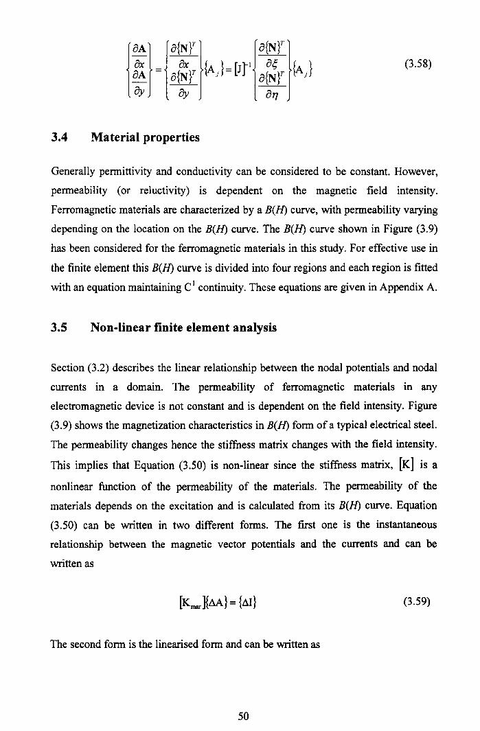
a{~}T a{~}Ta{~y {AJ= [Jjl a~y {AJ
ay aT]
(3.58)
3.4 Material properties
Generally permittivity and conductivity can be considered to be constant. However,
permeability (or reluctivity) is dependent on the magnetic field intensity.
Ferromagnetic materials are characterized by a B(ll) curve, with permeability varying
depending on the location on the B(ll) curve. The B(ll) curve shown in Figure (3.9)
has been considered for the ferromagnetic materials in this study. For effective use in
the finite element this B(ll) curve is divided into four regions and each region is fitted
with an equation maintaining Cl continuity. These equations are given in Appendix A.
3.5 Non-linear finite element analysis
Section (3.2) describes the linear relationship between the nodal potentials and nodal
currents in a domain. The permeability of ferromagnetic materials in any
electromagnetic device is not constant and is dependent on the field intensity. Figure
(3.9) shows the magnetization characteristics in B(ll) form of a typical electrical steel.
The permeability changes hence the stiffness matrix changes with the field intensity.
This implies that Equation (3.50) is non-linear since the stiffness matrix, [K] is a
nonlinear function of the permeability of the materials. The permeability of the
materials depends on the excitation and is calculated from its B(ll) curve. Equation
(3.50) can be written in two different forms. The first one is the instantaneous
relationship between the magnetic vector potentials and the currents and can be
written as
(3.59)
The second form is the linearised form and can be written as
50

(3.60)
where [Kmarl is the tangential or marginal stiffness matrix. If we know the flux
density everywhere, then we would be able to calculate the stiffness matrix [Kmar]instantly and directly. The flux densities are calculated by an iterative procedure using
a Newton-Raphson technique which is described in the next paragraph. {bJ is the
free MMF vector. For a linear case the value of the vector {bJ will be zero and then
Equation (3.60) will be similar to Equation (3.50). That is why linear problem is
treated as a special case of non-linear problem throughout this thesis. To calculate the
vector {bJ, a point PI is considered in the non-linear region on the B(1l) as shown in
Figure (3.10). If a tangent is drawn through PI as shown by a dotted line in Figure
(3.10), then there will be a negative value for field intensity. This is shown as M in the
figure. Based on the direction of the saturation there will be components of M. Once
the components of M are obtained the free MMF vector can be calculated using the
similar procedure explained in Section 3.3.4.2.
The Newton-Raphson procedure, an extension of the Newton method, is adopted
because of its quadratic convergence to solve non-linear problem in this analysis. It
works by guessing a trial solution, and then successively improving the "initial guess"
by using the slope of the B(ll) curve. Figure (3.10) shows a schematic representation
of the procedure adopted to solve the non-linear static electromagnetic problem using
the Newton-Raphson method.
The procedure starts with an initial guess of the permeability and this is shown as f.ig
in Figure (3.10). BT (x,y) and HT (x,y) are the flux density and field intensity
respectively corresponding to f.ig• M(x,y) is referred here as the free MMF which is
(3.61)
51

At each point in the domain a linear approximation is made to the magnetic
characteristics. The stiffness matrix and free MMF are calculated for this initial guess.
Once the stiffness matrix and the free MMFs are calculated, the magnetic vector
potentials are calculated using Equation (3.60). Now an excitation residue vector, {9t}is calculated using the equation
(3.62)
The nominal correction proposed by the standard Newton-Raphson procedure for
addition to the magnetic vector potential will be
(3.63)
The actual new magnetic vector potential is
(3.64)
Here a is a relaxation factor which helps to facilitate the convergence. Improvement
of convergence characteristics of Newton-Raphson method for nonlinear magnetic
field analysis by choosing the optimum relaxation factor is explained by Nakata
(1992) and Oapos and Oapos (1995). The procedure for updating the estimated vector
of potentials based on a known vector of excitation is continued until the norm of the
residue satisfies the convergence criteria.
3.6 Computer code for finite element analysis of electromagnetic
The previous sections mainly focus on the general procedure of finite element
modelling in electromagnetic field problems. A particular interest is devoted to the
modelling of magnetic material behaviour and to the coupling with the
electromagnetic field computation. The procedures described above are general in
nature and can be applied to the analysis of any electromagnetic systems.
52

Computational codes called MagFEA (Magnetic Finite Element Analysis) for two-
dimensional electromagnetic field problems have been developed in the MATLABTM
environment based on these procedures. The results are verified by a commercial
software called 'MEGATM' developed by the University of Bath, UK. The results
obtained from the MagFEA and MEGA for a simple electromagnetic device have
been presented in Appendix. Most of the numerical routines that have been used are
standard routines within MATLAB. This is the main reason for choosing MATLAB
for this study. MagFEA comprises a pre-processor where the model is built, a solver
where excitations are applied and responses are computed and a postprocessor, for
producing graphical output. The solver has the capability to solve linear as well as
nonlinear transient problem.
3.6.1 Pre-processor
In the pre-processor facilities are provided which assist the user in creating a
description of his model. The design of the pre-processor of MagFEA is generic and
can model any 2D geometry. Mesh generation is semi-automatic. At the first stage the
user has to identify the key regions of the model and then specify the discretisation
level. An isoparametric element is used to map the local element to the global
element. The procedure of mesh generation can be summarised as follows:
• User divides the meshable region into key regions (or elements).
• Generate information about the nodal coordinate of the key nodes and
connectivity of the nodes of the key region.
• Generate information about the material properties and excitation of individual
key elements.
• User decides the discretisation level depending on the requirement.
• Discretise individual key elements as per the discretisation level using
isoparametric elements.
The model comprises of seven arrays and these are KEYNODES, KEYELEMS,
KDIV, NODES, ELEMS, PERM, EXCT.
• KEYNODES comprises of three columns and stores the information about the
nodal coordinates of the key nodes of the domain to be discretised. The first
53

column stores the keynode labels, and the other two columns stores the x- and
y-coordinates respectively.
• KEYELEMS comprises of eleven columns. It stores the information about the
connectivity of the keynodes, indices for the material properties, excitation
and element types. The first eight column stores the connectivity of the
keynodes. Some of the entries of these eight columns will be zero if we use 4-
noded quadrilateral, 3-noded triangular and 6-nodes triangular elements.
• KDIV stores the information about the discretisation level and comprises two
columns. The number of rows of KDIV is equal to the number of key
elements. The first column stores the number of divisions along the local x-
axis and the second column stores the number of divisions along the local y-
axis of a particular key element.
• Similar to the KEYNODES, NODES comprises of three columns and stores
the information about the nodal coordinates of all nodes of the whole domain
once it is discretised. These columns store exactly the same information as the
columns ofKEYNODES.
• Similar to the KEYELEMS, ELEMS comprises of eleven columns and stores
the information about the connectivity of all nodes for the whole domain once
it is discretised. These columns store exactly the same information as the
columns ofKEYELEMS.
• PERM comprises of two columns and stores the information about the
material properties specified by the ninth column of ELEMS. The two
columns of a particular row represent the permeabilities along the two
orthogonal directions and they are !ixx and !iyy' In case of isotropic materials
J.lxx = J.lyy but in case of orthotropic materials !ixx *!iyy •
• EXCT stores the information about the excitation applied to the elements. The
excitations are mainly constant current density. This array is optional because
in most of the application of this study we do not have prior information about
the excitations in terms of current density.
54

3.6.2 Solver
The solver is capable of solving 2D magneto-static electromagnetic problems. An
excitation is applied as a current density. The solver is also capable of modelling
permanent magnets. To solve for the permanent magnet remanent flux, the relative
permeability and magnetization direction are provided as an input to the solver. Any
permanent magnet portions of the model are modelled using current distributions. The
solver has the following capabilities
• Linear and non-linear 2D magneto-static analysis of electromagnetic
system, electromechanical actuators, electrical machines.
• Steady state characteristics of electrical machines in general and
induction machine in particular.
• Transient solver including motion-induced eddy currents.
This solver also includes the coupling of electromagnetic equation to the mechanical
equations of motion, so that the movement of an electrical machine is accurately
simulated. The rotor and stator of an electrical machine are modelled completely
independently and combined at the middle of the airgap to take care of the rotor
movement. The solver re-meshes only the airgap regions to take care of the rotor
movement. A method where the solver does not have to be re-meshed to take care of
the movement is explained later Chapter 7.
3.6.3 Post-processor
In the post-processor the computed results from the analysis are displayed. The post-
processor has the following features
• Plot contours of the magnetic flux at any location in the finite element domain.
• Calculate and plot the flux densities along the two orthogonal directions at any
location in the finite element domain.
• Calculate and plot the magnetic stresses along the two orthogonal directions at
any location in the finite element domain.
• Calculate the forces along the two orthogonal directions.
55

3.7 Case studies for Static Unbalance Magnetic Pull (UMP)
This section presents three case studies to validate the non-linear finite element code
developed which is explained in the previous section and also to calculate static UMP.
In the following section the results from the finite-element code (MagFEA) are
presented. Static UMP is calculated for two different electrical machines. The first
one is a 2 kW, 3-phase induction motor. The configuration of the stator and
electromagnetic parameters of this motor are similar to the experimental rig discussed
in later chapters. The only difference between the two is the configuration of rotor.
Unlike the rotor in the experimental rig, the rotor in the machine studied here has non-
magnetic slot wedges. The numerical modelling code has the provision to study
machines with either magnetic or non-magnetic slot wedges.
3.7.1 Case study I: Unbalanced magnetic pull of an induction
machine
The first case study aims to calculate the static UMP of a 2 kW induction motor. The
main electromagnetic parameters of the motor are presented in Table (3.1). The stator
and rotor are modelled separately and discretised with eight noded quadrilateral
elements. These two meshes are connected at the middle of the airgap with six noded
triangular elements. Figure (3.11) shows the finite element mesh considered for this
study. Currents are applied at the stator windings which vary sinusoidally about the
machine periphery producing a four pole field in the motor. Forces are calculated
using the non-linear solver of MagFEA when 3-phase sinusoidal currents with peak
currents of 100A, 200A and 300A per slot respectively in the stator for different
eccentricities of the rotor. Induced currents in the rotor are not considered as the radial
force is calculated for the worst case of the motor. A contour plot of magnetic vector
potentials is shown in Figure (3.12) when a 3-phase current with a peak of 200A is
applied in the stator for a concentric rotor. Figures (3.13) and (3.14) show the normal
and tangential components of flux density in the middle of the airgap respectively for
the same operating current but with an eccentricity of 10% of the airgap. The
magnetic normal and shear stresses are calculated using Equations (2.23) and (2.24)
of Chapter 2 once the components of flux densities are known at the airgap. Normal
S6

and shear stresses in the airgap are shown in Figures (3.15) and (3.16) as a function of
the angular position.
The mean airgap for the above study is kept constant at 0.4 mm. Forces are calculated
by shifting the rotor from its central position along the positive x-direction as well as
along the negative x-direction. Because of the discretization there will be some
vertical force associated with this horizontal movement. Figure (3.17) shows the
horizontal and vertical forces per meter of axial length for different eccentricities
when 3-phase current with a peak of 200 A (per slot) is applied. For a 30% rotor
eccentricity a force of 1800 N per meter of axial length is generated. From Figure
(3.17) negative stiffness is calculated as 1.883 x 10⁶ (N/m) per meter of axial length.
From Figure (3.17), it is clear that force is varying quite linearly with eccentricities of
up to 30% of the airgap. Figure (3.18) shows the horizontal and vertical forces per
meter of axial length for 3-phase currents with different peaks per slot. The effect of
magnetic non-linearity in the iron is distinct from Figure (3.18). For a peak current of
300 A per slot, the force no longer varies linearly with the current. As the machine is
saturated the magnetic fluxes are distributed uniformly reducing the amount of
unbalance flux in the airgap and in turn reduces the unbalance force in the airgap.
3.7.2 Case study II: Unbalanced magnetic pull of a small high speed
permanent magnet alternator (PMA)
The second case study investigates UMP for a small high speed 14-pole permanent
magnet alternator with an overhung rotor. This case study serves as an excellent
example to demonstrate how severe the effects of UMP can be. It is found from this
small study that a significant reduction of critical speed is possible due to UMP. Thisreduction was not appreciated fully by the system designers during the mechanical
modelling of the alternator. The main parameters of the alternator are given in Table
(3.2).
The stator and rotor of the permanent magnet alternator are modelled separately using
eight-noded quadrilateral element and the two are combined by stitching the airgap
using six-noded triangular elements. Horizontal and vertical forces are calculated for
57

different eccentric position of the rotor in the same way as they were calculated for
case study I. In this case the excitation is considered from the permanent magnets on
the rotor. Stator currents are constrained to remain zero in this analysis. Figure (3.19)
shows the FE mesh considered for the analysis. The remanent flux density of the
permanent magnet material is 1.2 Tesla with and its relative permeability is taken to
be 1. Figure (3.20) shows the contour plot of the magnetic vector potential. Once the
model is solved using the non-linear solver of MagFEA the normal and tangential
components of flux density are calculated at the middle of the airgap. The airgap
radial thickness of the PMA is 0.635 mm. Figures (3.21) and (3.22) show the normal
and tangential components of flux density in the middle of the airgap of the PMA. A
normal component 0.65 Tesla can be achieved in the middle of the airgap for
remanent flux density of 1.2 Tesla of the permanent magnets. The normal and
tangential stresses at the middle of the airgap are shown in Figures (3.23) and (3.24)
respectively. Figure (3.25) shows the forces per meter of axial length along x-
direction for different eccentric positions of the rotor. The negative stiffness
calculated for the PMA is 7.276xl 05 (N/m) per meter of axial length.
3.7.2.1 Reduction of critical speed due to negative stiffness
As stated in Equation (2.11) of Chapter 2, the natural frequency of a coupled electro-
mechanical model can be calculated as
(3.65)
where Kmech is the mechanical stiffness and Kmag is negative stiffness due to UMP.
Equation (3.65) shows that due to negative stiffness the natural frequency is reduced.
True critical speed of the PMA is calculated for a wide range of mechanical stiffness
which is taken as multiples of the negative stiffness. Figure (3.26) shows the variation
of true critical speed of the PMA against the predicted critical speed only from
mechanical stiffness. Each predicted critical speed is associated with a particular
bearing deflection. Critical speed is 'zero' until the bearing stiffness is equal to the
negative stiffness. If the operating critical speed without negative stiffness is 25000
58

rpm, the reduction of critical speed is 6% if negative stiffness is considered. The
reduction of the critical speed is 20% if the operating critical speed is 15000 rpm.
3.7.3 Case study III: Investigation of tooth passing spatial
harmonics (TPSH) excitation with non-magnetic and
magnetic slot wedges
The third Case is an investigation carried out for a company considering the design of
a 2-pole generator for a defence application. The aim of this investigation is to study
the magnitude of the tooth passing spatial harmonics (TPSH) of the normal stress in
the airgap of a 2-pole generator with non-magnetic and magnetic slot wedges. The
dimensions of the slot are shown in Figure (3.27). The main parameters of the
generator are given in Table (3.3). Figure (3.28) and (3.29) show the finite element
mesh of one half of the machine. In these two figures 'cyan' colored regions represent
the slot wedge. Taking advantage of the symmetry only one half of the machine is
analyzed. The machine is solved for three levels of current density i.e. 5A1mm2,
10Almm2 and 15A1mm2 in the rotor slots for cases with non-magnetic and magnetic
slot wedge respectively. Figures (3.30) and (3.31) show the contour plots for a
machine with non-magnetic and magnetic slot wedge for a current density of 15
Almm2• Once the nodal magnetic vector potentials are known for the model, the
magnetic normal stress and shear stress are calculated from the normal and tangential
component of magnetic flux density. Figures (3.32) and (3.33) show the normal and
tangential components of magnetic flux density in the airgap with non-magnetic slot
wedge for a current density of 15 Almm2• Similarly, Figures (3.35) and (3.36) show
the normal and tangential components of magnetic flux density in the airgap with
magnetic slot wedge for a current density of 15 Almm2• Figures (3.34) and (3.37)
show the normal components of magnetic normal stress in the airgap with non-
magnetic and magnetic slot wedge respectively for a current density of 15 Almm2•
The magnetic normal stress is reduced because of the use of magnetic slot wedge and
this is clearly seen from Figure (3.37). Taking the advantage of symmetry, the
magnetic normal stress is calculated for angle 0 to 2n. The TPSH component of
magnetic normal stress is calculated by taking an FFT of the normal stress. It is found
that incorporating magnetic slot wedges in place of non-magnetic slot wedges reduces
59

the magnitude of the tooth passing spatial harmonics of the normal stress by 60%.
There is a slight loss of performance associated with the inclusion of magnetic slot
wedges since they provide a magnetic "short-circuit" around the rotor conductors.
3.8 Magnetic Pull (UMP) for overhung machine
Figure (3.38) shows a schematic view of an electrical machine with an overhung rotor
and Figure (3.39) shows the corresponding equivalent system. The extended length
and the weight of the overhung rotor cause a considerable amount of unbalanced
magnetic pull. From the Figure (3.39) the equivalent stiffness of the system is
K _ KMECH_STATOR X KUMPEQUIV - ( )
KMECH_STATOR + KUMP
(3.66)
where KMECH_STATOR is the mechanical stiffness of the stator and KUMP is the negative
stiffness because of UMP. If the mechanical stiffness of the stator, KMECH_STATOR is
large compared to the negative stiffness of the rotor, KUMP then KUMP is the
equivalent stiffness. However, if KMECH_STATOR ::::KUMP then the stiffness of the rotor
reduced significantly and there is a tendency to pull the stator towards the rotor.
3.9 Summary of the chapter
The basic procedures of finite element analysis of electromagnetic devices are
discussed. The relationship between the nodal currents and the magnetic potentials
has been established. For a given current density we can calculate the magnetic
potentials. The procedure for calculating resistance matrix of an electromagnetic
device using the finite element method is also discussed. Using these procedures a
non-linear finite element code, called MagFEA, is developed. Three case studies have
been performed using this FE code. The first two case studies investigate the static
UMP and the third case study investigates the effect of the tooth passing spatial
harmonics in case of the magnetic and the non-magnetic slot wedge.
60

(-I,I).4~ .... (1,1)..--------~--------~~~ : 3~~I1I
t :.,,1
1- - - - - - - - -1- - - - - - - --
I ~~II1I1I1
(-1, 1).4~
(1, 1).4~
IIII
i II
." III---------r--------
(0,0) : q--7IIIIII.4. .4'"~.
(-1, -1) (1, -1)
Figure (3.1): Master element
y
o x
Figure (3.2): Isoparametric element
~. (1,-1)
Figure (3.3): Node point ordering of a 4-noded quadrilateral element
61

(-1,1) (0,1 ) (1,1)
2 ,6 3,,,j',T/'
(-1,0) ,(1,0)-------~--------
5 , ;~ 7,,,,,'8 4
(-1,-1) (0,-1)(1,-1 )
Figure (3.4): Node point ordering of a 8-noded quadrilateral element
(0,1)
(1,0)(0,0)
Figure (3.5): Node point ordering of a 3-noded triangular element
62

(0,1)
(O,Y2
(0,0) (Y2,O) (1,0)
Figure (3.6): Node point ordering of a 6-noded triangular element
I-Alnico2 -Ferrite3 -Samarium-Cabalt4 - Noodymium-Iroa-Boroa
s»1.2
0.8
0.4
200 H(lcAIm)
Figure (3.7): B(H) curves for some permanent magnet (Bastos and Sadowski,2003)
63

H
Figure (3.8): Magnetisation curve for a permanent magnet
1.5r----,---,----,---,----,---r----,-----,
125 -,
- _I _
,-,----_._----
-- - - - - + - - - - - + - - - - - -! - - - - - -I - - - -,
025, , ,
- - - - - "I - - - - - "I - - - - - - - - - - - -I - - - - -
100 200 300 400 500 600~c field imemity,H(inA17m)
700 800
Figure (3.9): Magnetization characteristics in B(H)-form ofa typical electrical steel
64

H
Figure (3.10): Schematic representation of solution procedure of non-linear static
electromagnetic problem
Table (3.1): Parameters of the 2 kW induction motor
Parameters
Number of polesNumber of phase
Number of stator slotsOuter diameter of the stator [mm]Inner diameter of the stator [mm]
Number of rotor slotsOuter diameter of the rotor [mm]
Airgap [mm]Rated voltage [V]
Rated frequency [Hz]Rated power rkWl
65
Value
4336153933292.20.4415502

Figure (3.11): FE mesh of the induction motor considered for case study 1
Figure (3.12): Contour of magnetic vector potential when a sinusoidal current when 3-
phase current with a peak of 200 Amps (per slot) is applied.
66

0.5
-0.5 -
-1
1
6
o
3 4Angle (rad)
Figure (3.13): Normal component of flux density in the middle of the airgap when 3-
o I 2 5
phase current with a peak of 200 Amps (per slot) is applied.
0.4,------,------r------,------r------,------~
0.3
0.2
0.1
o ~Il
- -
1\
J _
_04L_----~----~------~-----L------L-----~. 0 1 2 3 4 5 6
Angle (rad)
- , I
-0.1
-0.2
-0.3 - -- - 1 - -
Figure (3.14): Tangential component of flux density in the middle of the airgap when
3-phase currents with a peak of 200 (per slot) Amps is applied
- -'
-- - -
67

4
ok-J-:. - -
~,~
-/'1 -- - -
rl
~ U1-.,.c-< - - - -Irv--
2 3 4 5 6Angle (rad)
o 1
Figure (3.15): Normal stress at the middle of the airgap when a sinusoidal current
when 3-phase current with a peak of 200 Amps (per slot) is applied
1.5 - - - - - -
.-Ne0.5Z
'-'I:IlI:Il 0~'"' ~....en'"'~ -0.5~..c:en
-1 _, ______ L
-1.5 _______ L __
-20 1
___ .1.. -1- -1 .-<'_ ...J _
__ 1.. ~ _..._ ~---,
I I
, -,
J .• ~.~.
J_ _
- -
- - ~-,
--
2 3 4Angle (rad)
5 6
Figure (3.16): Shear stress at the middle of the airgap when a sinusoidal current when
3-phase current with a peak of 200 Amps (per slot) is applied
68

2500.0
2000.0
1500.0
1000.0
,.-. 500.0Z'-(!) 0.0
---uCl -500.0u,
-1000.0
-1500.0
-2000.0
-2500.0-30
.---- --- .-.-
-10 o 10 20-20
Eccentricity (%age of airgap)
30
Figure (3.17): Horizontal and vertical force versus eccentricity for the induction
machine considered for Case Study I when 3-phase currents with a peak of 200 Amps
(per slot) is applied
2500.0
2000.0
,.-. 1500.0Z'-(!)o.... 1000.00u...
500.0
0.050
•100 150 200 250 300
Currents per slot (A)
r+Fxl~
350
Figure (3.18): Horizontal and vertical forces for 3-phase currents with different peaks
(per slot) in the stator for the induction motor considered for case study I
69

Table (3.2): Parameters of the permanent magnet alternator
Parameters Value143213.236.550.01.21.0
0.635
Number of polesNumber of phase
Number of stator slotsThickness of the permanent magnet [mm]
Outer diameter of the rotor [mm]Outer diameter of the stator [mm]
Remanent flux density of permanent magnet [Tesla]Relative permeability of the permanent magnet
Airgap [mm]Mass of the rotor which includes magnet, sleeve, carrier,
nut, and oil flinger [kg]Length of the rotor [mm]
Rated frequency [Hz]
0.8366750
Figure (3.19): FE mesh of permanent magnet alternator (PMA)
70

Figure (3.20): Contour plot of magnetic vector potentials of the PMA considering
permanent magnet excitation only
0.8
0.6
0.4
0.2~~rfJC) 0r-<:»
c:co-0.2
-0.4
-0.6- --
I
-0.80 2 3 4 5 6
Angle (rad)
Figure (3.21): Normal component of flux density in the middle of the airgap of the
PMA
71

0.6
0.4
~CIJ 0.2~'-'
af,
o ,} ~ -) -~ -)1 ~ } ~ )' -~ - ) -,~ _,)1 ~
-0.2IC . . ..
-04~----~----~-----L----~----~~----~. 0 1 2 3 456
Angle (rad)
Figure (3.22): Tangential component of flux density in the middle of the airgap of the
PMA (when the rotor is concentric with the stator).
5xlO2.5,-----~----~----~----~----~------~
I
2 A ~. A _ It _ '-~ It: A A __ ~ A _ ._ ~
-1 ~- - - - -
-1.5 _ - . - - - _.
-23 60 2 4 5
Angle (rad)
1.5
oc;a5 -0.5Z
1 -,
I..
I -
Figure (3.23): Normal stress in the middle of the airgap of the PMA
(when the rotor is concentric with the stator)
72

1.5
1.-"IS
0.5Z'-'CIlen 0~......
Cf.l..~ -0.5~..cCf.l
-1
-1.5
-20
- ..
,
-
. -
...
-- - - .-
5 6
Figure (3.24): Shear stress in the middle of the airgap of the PMA
(when the rotor is concentric with the stator)
1 2 3 4Angle (rad)
3000r-----~----~----~----~----~--__,
2000 - - -- -
z'-'I:.9 1000-(,)e:.a>< 001)I:o";j~ -1000e&
-2000
-300~0
,-"------------- ,,----------------
____ 1 -
,
~- -,
30-20 -10 o 10 20
Figure (3.25): Forces on the rotor along x-direction for different eccentricities in case
of PMA
Eccentricity (%age of air gap)
73

Equivalent bearing deflections
.3CXX)() 21 micron
-~.~.....·co 50002~
I_J
Figure (3.26): True critical speed when negative stiffness due to UMP is also
considered along with mechanical stiffness versus predicted critical speed of the
PMA.
1CXXXJ 15000 20000
Critical speed with only mechanical stiffness (rpm)
74
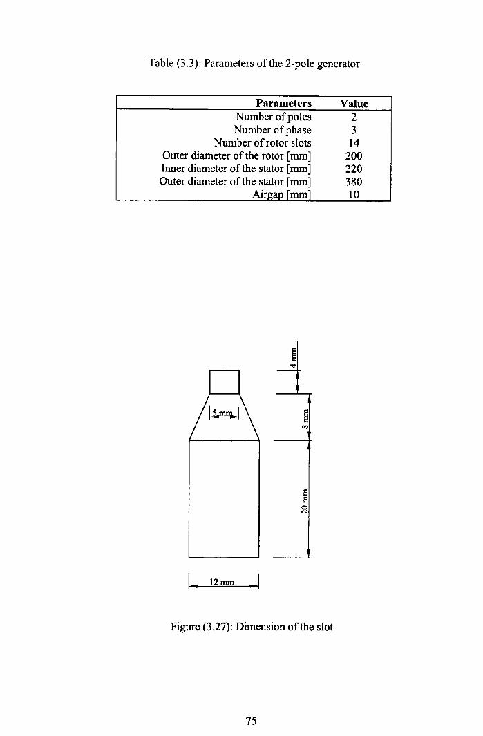
Table (3.3): Parameters of the 2-pole generator
Parameters ValueNumber of polesNumber of phase
Number of rotor slotsOuter diameter of the rotor [mm]Inner diameter of the stator [mm]Outer diameter of the stator [mm]
Airgap [mm]
I.. 12mm .1
Figure (3.27): Dimension of the slot
75
231420022038010

figure (3.28): A fE mesh
figure (3.29): A fE mesh
76

Figure (3.30): Flux contour with non-magnetic slot wedge with current density of 15
Azrnnr'
Figure (3.31): Flux contour with magnetic slot wedge with current density of 15
Azrnrn''
77

0.8
0.6
0.4
,-... 0.2cISr;;Q) 0r--.._,c
CQ -0.2
-0.4
-0.6
-0.8
-10 0.5 1.5 2 2.5 3
angles (rad)
Figure (3.32): Normal component of flux density in the airgap with current density of
15Azmm' for non-magnetic slot wedge
0.8
0.6 - .
0.4
.- 0.2cISr;;~ 0.._,c
CQ -0.2
-0.4
-0.6
-0.8 -
0
,---_--_._-- ,
,--1- ----"T ..
31.5 2angles (rad)
Figure (3.33): Normal component of flux density in the airgap with current density of
15 Almm2 for magnetic slot wedge
0.5 2.5
78

0.14
0.12
0.1
-- 0.08..:s"-l~
E-<'-"
00.- 0.06
0.04
0.02
00
)~_V _V_V V_ V_V \ ._ ~ -
0.5 2.5 31.5 2angles (rad)
Figure (3.34): Tangential component of flux density in the airgap with current density
0.07
0.06
0.05
--- 0.04.s"-l
~'-" 0.0300.-
0.02
0.01
of 15 Nmm2 for non-magnetic slot wedge
31.5 2angles (rad)
Figure (3.35): Tangential component of flux density in the airgap with current density
0.5 2.5
of 15 Almm2 for non-magnetic slot wedge
79

1.5 2angles (rad)
Figure (3.36): Normal stress in the airgap with current density of 15 Azmm' for non-
X 105
4
3.5
3,-._Ne...... 2.5Z'-'
'" 2'"Q)....-Cl)ca 1.5e....0Z
0.5 -
0
0 0.5 2.5
magnetic slot wedge
X 1053
2.5
,-._ 2NeZ'-'
'" 1.5<I"l
~-(/)cae....0Z
0.5
3
o 1.5 2angles (rad)
2.50.5 3
Figure (3.37): Normal stress in the airgap with current density of 15 Almm2 for
magnetic slot wedge
80

Table (3.4): Fourier coefficients of the normal stress in the airgap for different levels
of currents in the rotor slot
Normal stress in case of Normal stress in case of magneticnonmagnetic slot wedges at the slot wedges at the tooth tip
tooth tip
Spatial Current density in the rotor slots Current density in the rotor slotsHarmonics
5 10 15 5 10 15(Azrnrrr') (Almrn2) (Azmm'') (Azmnr') (Azmrrr') (Almrn2)
TPSH-6 7.3515E2 2.4344E3 3.8671E3 2.0870E3 3.3518E3 4.9412E3
TPSH-4 1.9142E3 4.9760E3 5.6994E3 1.2201E3 2.5845E3 3.4724E3
TPSH-2 3.6368E3 7.7403E3 9.4927E3 1.8937E2 3.7520E3 5.8764E3
TPSH 4.5649E3 1.2169E4 1.5723E4 3.9895E3 5.5286E3 5.6631E3
TPSH+2 3.1310E3 7.1593E3 8.2507E3 2.32166E 6.5880E3 8.6818E33
TPSH +4 5.6454E3 1.4287E4 1.7651E4 2.1202E3 2.4431E3 2.0911E3
TPSH+6 1.1245E3 3.0872E3 3.5190E3 1.0838E3 1.5152E3 1.5505E3
TPSH - Tooth Passing Spatial Harmonics
81

Rotor
Stator
Bearing 1 Bearing 2
Figure (3.38): Schematic view of an electrical machine with an overhung rotor
KMECH-ROTOR KUMP KMECH_STATOR
Figure (3.39): Equivalent system
82

Chapter Four
Co-ordinate Transformations Used in the Magnetic
FEA
4.1 Introduction
The 2D finite element analysis of electromagnetics explained in the previous chapter
is very general in nature. There, the view was taken that FEA would be used to create
an instantaneous relationship between nodal currents and nodal potentials. This
relationship takes the general form
{A}= f{{I}) (4.1)
where {A} = vector of magnetic potentials at nodes
{I}= vector of nodal currents
In other words the magnetic FEA that is used here is magneto-static. In the case of a
linear magnetic system
(4.2)
where [K] is the stiffness matrix
Electrical machines are electromagnetic devices with very complex geometries and
phenomena, having moving parts, magnetic saturation and induced currents. Their
simulations by finite element methods require special consideration. In the previous
chapter it was assumed that the currents were known and these were specified by
setting current densities in the domain of the analysis.
83

The FE models used throughout this work have been 2D. Each model comprises a
large number of nodes (typically 10,000) and these nodes are connected by finite
elements (often numbering around 3,000). In a fully general view of 2D magnetic
FEA, a single nodal current can be associated with every single node and also a single
magnetic potential can be associated with each. If the FEA formulation was intended
to capture eddy-currents intrinsically, each node would have had to be allowed three
components of the magnetic vector potential. Chapter 3 explained why all induced
currents were going to be modelled explicitly and why this (eddy currents)
formulation was not chosen.
This chapter addresses coordinate transformations of two basic types.
• Transformations that express the full length vector of nodal currents in terms
of a reduced length vector.
• Transformations that express the full length vector of nodal potentials in terms
of a reduced length vector.
It will be seen that the transformations are applied in stages with each stage reducing
the number independent variables (entries) in the vector of currents (potentials). Each
time that there is a reduction in the number of currents (potentials) a constraint of
some description is, in effect, applied. In some cases the constraint is known first and
the stage of the transformation is designed so as to satisfy that constraint. In other
cases, the main purpose of the stage of transformation is to reduce the computational
burden of working with the model. Then the transformation stage is designed such
that the constraints which are applied have the least impact on the fidelity of the
model.
In this chapter different transformations are used which transform the independent
terminal currents of the stator to nodal currents in the stator and also transform the
very large number of rotor nodal currents to the rotor bar currents. These
transformations are used in the subsequent chapters to calculate the steady state
currents from the electrical dynamics and also during the coupling of the
electromagnetic dynamics with the mechanical dynamics.
84

4.2 General principles of the coordinate transformations
Sometimes we use a formal method to obtain the transformation matrix and
sometimes by inspection. For both nodal currents and nodal magnetic potentials, we
will come across sets of constraints which must be applied. These are discussed
specifically in later sections but a single treatment can be outlined here. Because we
encounter the situation most commonly in connection with currents, we use that
situation here.
Let {Io} represent a "full length" vector of currents. If there are nodal currents, then
there is a corresponding vector {Ao} of magnetic potentials having the same length.
In a fully nonlinear model we have (at any instant)
{Ao}= j{{Io }) (4.3)
But it is always possible to find a linearised form to this as
[K]{Ao}= {Io}+ {bo} (4.4)
where [K] is the "tangential" or "marginal" stiffness and {bo}is the vector of free
MMF. Some constraints are known to apply to {Io}in the form
(4.5)
It is always possible to enforce these constraints by introducing the coordinate
transformation
(4.6)
where the matrix [r] must satisfy two requirements. where [r] is any matrix selected
in order that
85

• [Ej'[T]= 0
• [y][Yj' non-singular where [Y] := [E T]
There are several methods by which such transformation matrices may be found and
each of these will result in a different matrix, [T]. If any matrix [T] has been found
satisfying the above criteria, a number of alternatives [T1 may be found through
[T1= [T] [x] where [x] is any square invertible matrix of the appropriate dimension.
We now describe one method commonly used in Finite Element analysis for
developing the transformation. This method is highly efficient and it has good
properties of numerical stability. It deals with one constraint at a time and the final
transformation, [T], is developed as the product of p intermediate transformations,
ITp J where p is less than or equal to the number of constraints (columns in [E]). Each
[Ti] is effectively an identity matrix with an additional row inserted.
(4.7)
For reasons which become clear shortly, we employ a duplicate notation for [E] here
and we refer to that also as [Eo]. The number of rows in [Eo] equals the number of
degrees of freedom in the original system and is denoted no. Matrix [T1] has
dimensions (no x (no - 1)) and it is found by considering only the first column of
[Eo]. Let k be the position of the entry having the largest absolute value in this
column. [T1] can then be described entry-by entry as follows:
• [TJU, i) = 1 '<:/ 0< i < k
• [T1]U, i) = 1 '<:/ 0< i < k, i »] < no
• [1:)(k J] ~ ( - [EolCi, 1)J if 0 <j < kI' [Eo](k,I)
• [1:)(k ] ~ ( - [EolCi +1,I)J if k ~j < noI'] [Eo](k,I)
• [T1]U, i-I) = 1 '<:/ i>k
• [T1](i,j) = 0 Tt i > k, (i - 1);t j < no
86

Example (4.1): A simple example illustrates this nicely. Consider the case of a 6
degree of freedom system to which a single constraint is applied with [Eo] given by
[Eof =[2 -10 6 -4 5 20]
The sixth entry here has the largest absolute value and hence k = 6. Then
1 0 0 0 00 1 0 0 0
[Tl]=0 0 1 0 00 0 0 1 00 0 0 0 1
-0.1 0.5 -0.3 0.2 -0.25
The procedure for multiple constraints is a very small extension. Having found [Tl],
calculate [Elf = [Eof[TJ The first column of [El] contains only zeros and requires
no further work. The next step, finding [T2], proceeds precisely as the first step except
that [El] is used in place of [Eo] and its second column is considered.
Example (4.2): Consider the case of a 6 degree of freedom system to which two
constraints are applied with [Eo] given by
[2 -10 _6
2-84 5 2
00]
[Eor = 4 5 1
Proceed as in the previous example to find [Tl]. Then evaluating [ElY = [EoY [TJ
yields
87

Evidently, the first constraint requires no further attention. The second column of [El]
informs the determination of [T2] which emerges as
1 0 0 00 1 0 0
[T2Y = 0 0 1 0-0.5 -0.625 0.25 -0.1250 0 0 1
The product [T]= [TIHT2] is then determined easily. The procedure here can be
applied for any number of constraints. In some cases, the constraints are not all
independent. A particular case of this may be encountered in an electric circuit shown
in Figure (4.1) where each one of 5 different nodes produced a different constraint but
there are only 4 degrees of freedom in the original system and it transpires that only 4
of the constraint equations are independent. When the procedure described here is
applied to such cases, after [T4] and [E4] have been obtained, it is found that all
columns of [E4] are zero. The fact that its first four columns comprise zeros is not
surprising. The fact that all other columns comprise zeros points to the lack of
independence in the original constraints. In order to prevent round-off errors from
introducing spurious constraints, an account should be kept of the original magnitudes
of the columns of [Eo] and compared against the magnitudes of [E,] after the general
step i. The process is complete when all of these magnitudes are very low compared
with their original values.
4.3 Transformations of the stator currents
Most of the stators in electrical machines are powered by a three phase supply and it
is usual that only three independent currents are required to describe fully the currents
flowing in the stator. In ~-connected machines or Y-connected machines with a
floating star point only two currents are needed. Similar constraints also exist in the
case of wound rotors. Arrangements must be put in place in our stator model to
accommodate a transformation of three phase currents to the nodal currents.
88

Also, in the later part of this thesis while validating out numerical model we have
used a special kind of winding scheme, which can be used as a passive reduction of
unbalanced magnetic pull along with its torque producing capability. Unlike the usual
winding scheme this particular winding scheme has six stator currents. Amongst these
three are the phase currents and other three are so-called levitation currents. For a
concentric rotor where magnetic fields are symmetric the levitation currents are zero.
This is explained in detail in later chapters.
The full set of nodal currents in the stator is transformed to the terminal currents in
five different stages. Figure (4.2) shows a schematic of the different transformations.
The following subsections discuss each transformation separately. To illustrate the
transformations of the stator currents a 4-pole induction machine is considered. The
stator of the machine and its winding connections are shown in Figures (4.3) and
(4.4). The machine has 36 stator slots. The winding is a dual layer distributed winding
with fractional pitch coils. The pitch of each coil is (6/9) or 120 electrical degrees.
4.3.1 Transformation of the full set of nodal currents in the stator
to the nodal currents correspond to the conducting regions in
the stator (Stage I)
In the FE models every single node has an associated nodal current but many of these
are always zero. Non-zero currents are associated only with those nodes which are
either boundary or within the conducting regions of the FE model. The full set of
nodal currents in the stator is transformed to a smaller set of nodal currents
corresponding to the nodes of the conducting regions. This is accomplished by the
following transformation:
(4.8)
where {Isne} is the full set of nodal currents and {ISene} is the smaller set of nodal
currents corresponding to the nodes of the conducting regions. The number of
columns of the transformation matrix, [TS1] will be the same as the number of entries
89

of {ISene}. Most of the entries of [Ts1] will be zeros as majority of the nodes will not
carry currents.
Consider any part of the domain of a stator as shown in Figure (4.5), which has
conducting as well as non-conducting regions. This part is descretised with three 4-
noded finite elements and element 2 is the only conducting region. Suppose iI, ii. i3 ...
is are the nodal currents corresponding to nodes 1, 2, 3, ... 8 respectively, the
transformation in this case will be
il 0 0 0 0i2 0 0 0 0i3 1 0 0 0 i3i4 0 1 0 0 i, (4.9)=is 0 0 1 0 isi6 0 0 0 1 i6i7 0 0 0 0ig 0 0 0 0
4.3.2 Transformation of the nodal currents corresponds to the
conducting regions to the coil side currents in the stator (Stage
II)
In this transformation the nodal currents corresponding to the nodes of the conducting
regions, {Isene} are transformed to "coil-side" currents. A coil-side represents a
conducting region in a particular stator slot having, in effect, a constant current
density. In Figures (4.3) and (4.4), +al represents one coil side. Since the example
machine has 36 slots with dual layered windings, it will have 72 entries in the coil
side current vector. This transformation is explained with the following illustration.
Consider a stator slot with double layer windings as shown in Figure (4.6). Here the
two layers are distinguished by two different colours. Each layer is discretised with
finite elements. Figure (4.7) shows layer 1 having been discretised with two 8-noded
finite elements. Currents corresponding to layer 1 have one entry in the "coil side"
90

current vector. Suppose i}, iz. is ... i13 are the nodal currents corresponding to nodes 1,
2, 3,... 13 respectively as shown in Figure (4.7). {I;} and {In are the currents for
elements l' and 1"respectively. Assuming constant current density in the region of one
set of coil
a'il
1
AIi2
a2AI
i3ajAi
i4a'4 (4.10)AI {I; }= asis AI., a''6 6
AI., a;'7 AI., as'8 AI
and similarly
." a~
'6 A~
." a;
'7 A~." a'8's A~
i9 a9 (4.11)Ai {I~}= aioiIO Afill
ailA~
i12 ai2Af
il3 ailA~
where a;, a;, a~ are the areas associated with the nodes correspond to element l'
and a;, a;, a;3 are the areas shared by nodes correspond to element 1" and also
note that a; + a; +...+a~= A;, a; + a; + ...+ a;3= A; . Here A; and At are the areas
for elements l' and I"respectively. These areas are determined by the corresponding
shape functions. i~, i; and i~are the nodal currents of nodes 6, 7, and 8 respectively
contributed by element l' only. i:, i; , and i: are the nodal currents of nodes 6, 7, and
8 respectively contributed by element l' only. Nodes sharing more than one element
91

such as nodes 6, 7, and 8 will have contributions from the two elements. Finally these
thirteen nodal currents can be written in terms of only one slot current as
il a~
i2 a~
= {I'} (4.12)i7 (a;+a7~
il3 a~V;
Following this, the nodal current in a particular stator slot can be written in terms of
its corresponding "coil side" currents by transformation matrix, [TS2].
(4.13)
Here {ISese } is the "coil-side" current vector. Since the stator has 36 slots with dual
layer of winding, it has 72 coil sides and 72 current variables entries. The number of
columns of [TS2] is the same as the number of coil side current variables.
4.3.3 Transformation of the coil side currents to the full coil
currents in the stator (Stage III)
Every full coil current corresponds to two half-coil currents. In Figure (4.4) ar
represents one full coil. This transformation imposes a constraint that current going
down in slot -al is equal in magnitude to the current coming up in slot +al (+al is not
shown in the figure) but opposite in sign. This transformation can be written by
inspection. The transformation can be written as:
(4.14)
92

where {Isfcc}is the vector of full coil currents. For the machine considered {Isfcc}will
have 36 entries. The size of the transformation matrix [Ts3] is (72x36). We can write
the transformation for this as
i+al 1 0
t.; -1 0 ...h}i; = 0 1 (4.15)i_a2 0 -1
where i: ' i.; ' i+a2 ' i_a2 are the coils side currents of coil sides + a), - a), + a2 , and
- a2 respectively and ia1, ia2 are the full coil currents of full coils a), and a2
respectively [refer Figures (4.3) and (4.4)].
4.3.4 Transformation of the full coil currents to the coil group
currents in the stator (Stage IV)
The six full coils ai, a2, ai, aa, as, and a, together form one "coil group" and since they
are connected in series as per the winding scheme shown in Figure (4.4), they have
the same currents. This transformation transforms the coil currents within {ISfCC} to the
coil group currents. The transformation is:
(4.16)
where {Iscgc}is the vector of coil group currents. The vector {lsfcc}has 6 entries. The
size of the transformation matrix [Ts4] is (36x6).
93

ia, 1 0 0 0 0 0
0 0 0 0 0
ia6 1 0 0 0 0 0iaa, 0 1 0 0 0 0
0 0 0 0 0
iaa 0 1 0 0 0 06ib, 0 0 1 0 0 0 ia
0 0 0 0 0 iaaib6 0 0 1 0 0 0 ib
=: [Ts4 ]{IsegJ=ibb, 0 0 0 1 0 0 ibb (4.17)
0 0 0 0 0 icibb6 0 0 0 1 0 0 icct; 0 0 0 0 1 0
0 0 0 0 0
i: 0 0 0 0 I 0
ice I 0 0 0 0 0 I0 0 0 0 0
i; 0 0 0 0 0 1
In Equation (4.17) ia" "., ia6, iaa" "., iaa6 are the full coil currents of full coils aI'''''
a6, aa., ... , aa, respectively corresponding to phase A. Currents with subscripts b
and c correspond to phases Band C respectively.
4.3.5 Transformation of the coil group currents to the terminal
currents (Stage V)
This transformation converts the 6 coil group currents to 3 terminal currents. The
transformation is
(4.18)
where {Is} is the vector of terminal or phase currents. The vector {Is} has 3 entries of
the three phase currents as:
94

{iAPh}
{Is}= ~BPh'Cph
(4.19)
The size of the transformation matrix [Tss] is (6x3). If the resistance of the six coil
groups are same and also the EMFs due to changing magnetic field in the two coil
group in a particular phase are same then we can write
ia 1 0 02"iaa 1 0 02" f~}ib 0 1 0 (4.20)2"
~BPh =: [Tss HIs}=ibb 0 1 02"i, 0 0 j_ 'Cph
2
iCC 0 0 12"
where ia, iaa, ib, ibb, ie' icc are the coil group currents and iAph' iBPh' iCph are the three
terminal currents. Finally the overall transformation can be written as
(4.21)
The final transformation matrix can be written as
(4.22)
where [Ts] is the transformation matrix which determines the transformation of nodal
currents to the terminal currents.
4.3.6 Transformation of the coil group currents according to the
bridge windings
In a usual winding scheme (similar to Figure (4.4» there will be three independent
stator phase currents but in some special windings scheme such as (Khoo, 2005) there
95

can be more than three currents. Here without going about the detail of the bridge
configured winding scheme introduced by Khoo (2005), an explanation is given for
the transformation of stator slot currents to the independent stator phase currents. One
reason for choosing this winding scheme for explanation is that it is used in the
experimental rig developed to study electromechanical interaction of an induction
machine. Another reason is that it contains more than three currents. Some features of
this winding scheme are explained in Chapters 7 and 8. Figure (4.8) shows the
equivalent bridge connection for the winding connection shown in Figure (4.3). The
branch currents, phase currents and the levitation currents are shown for phase A in
the figure. Unlike the conventional winding scheme, this particular winding scheme
has one "levitation current" per phase. The usage of this levitation current will be
explained in detail in Chapter 5. A transformation matrix which transforms all the slot
currents (or branch currents as shown in Figure (4.8)) to the phase currents and
levitation currents is required. Assuming the same resistance in each branch of the
bridge the transformation matrix for the phase A is calculated as follows,
iA 1 12" 2"
iB 1 _1. fAp>} (4.23)2" 2=iC 1 1
2" -2 IAlev
iD 1. 12 2"
iA, iB, tc, and iD are the currents in four branches of the bridge for phase A. It is also
assumed here that EMFs due to changing magnetic fields are identical for each branch
of the bridge. Similar transformations shown in Equation (4.23) are also obtained for
phases B and C. These comprise a different transformation matrix [TssJ, similar to
[Tss] explained in Section (4.4.5), which transforms the stator coil group currents to
the phase currents. iA, iB, ic, and iD are the four entries of the current vector {Iscgc}.
Similar currents variables are obtained for phases B and C. Unlike the current vector,
{Is} shown in Equation (4.21), the vector {Is}there will have six entries when we use
the bridge configured windings, i.e.
96
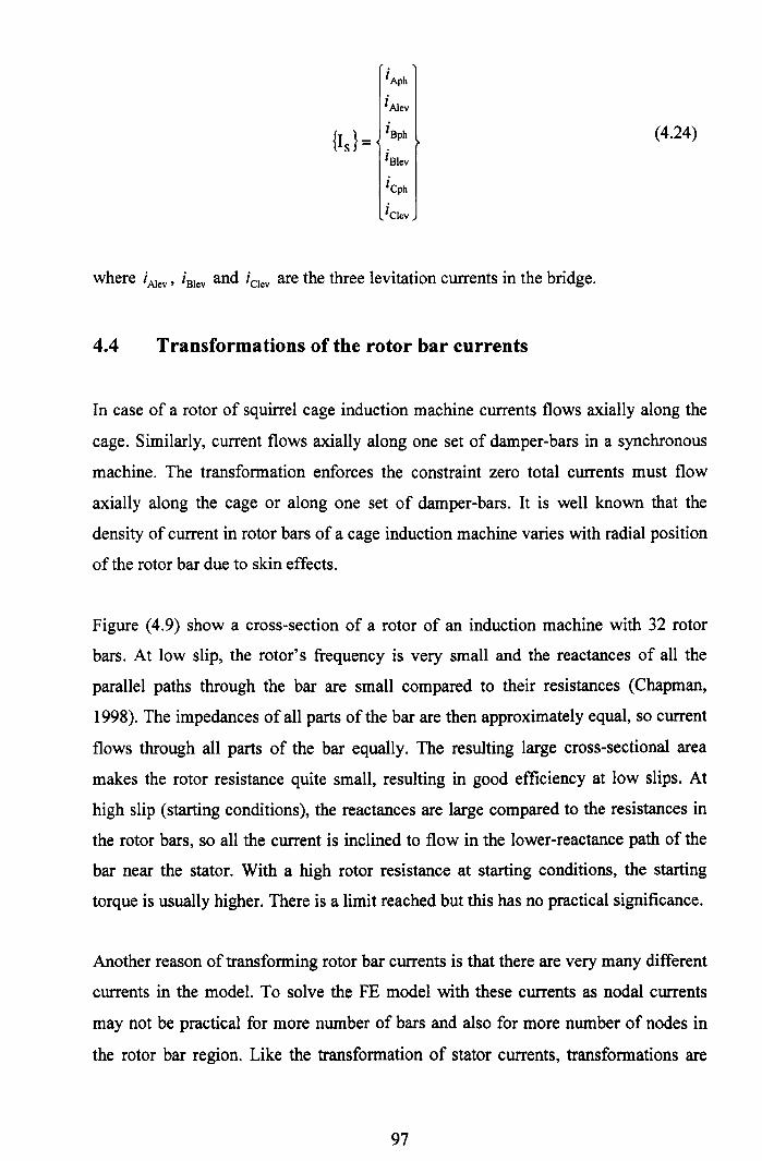
iAPhiAlev
{Is}= iSph (4.24)iSleviCphiClev
where iAlev s iSlev and iClev are the three levitation currents in the bridge.
4.4 Transformations of the rotor bar currents
In case of a rotor of squirrel cage induction machine currents flows axially along the
cage. Similarly, current flows axially along one set of damper-bars in a synchronous
machine. The transformation enforces the constraint zero total currents must flow
axially along the cage or along one set of damper-bars. It is well known that the
density of current in rotor bars of a cage induction machine varies with radial position
of the rotor bar due to skin effects.
Figure (4.9) show a cross-section of a rotor of an induction machine with 32 rotor
bars. At low slip, the rotor's frequency is very small and the reactances of all the
parallel paths through the bar are small compared to their resistances (Chapman,
1998). The impedances of all parts of the bar are then approximately equal, so current
flows through all parts of the bar equally. The resulting large cross-sectional area
makes the rotor resistance quite small, resulting in good efficiency at low slips. At
high slip (starting conditions), the reactances are large compared to the resistances in
the rotor bars, so all the current is inclined to flow in the lower-reactance path of the
bar near the stator. With a high rotor resistance at starting conditions, the starting
torque is usually higher. There is a limit reached but this has no practical significance.
Another reason of transforming rotor bar currents is that there are very many different
currents in the model. To solve the FE model with these currents as nodal currents
may not be practical for more number of bars and also for more number of nodes in
the rotor bar region. Like the transformation of stator currents, transformations are
97

needed for the rotor bar currents so that we can represent the full set of nodal currents
of the rotor with fewer current variables. If current densities were constant, we would
use only one current variable per bar. As mentioned above current density in a rotor
bar is a function of radius and radial depth of the rotor. To take care of these effects
provisions have to be made in the numerical model. The transformations from the full
set of nodal currents in the rotor to the smaller number of current variables are
achieved in four different stages. These stages are shown in Figure (4.10).
4.4.1 Transformation of the full set of nodal currents in the rotor to
the nodal currents corresponding to the conducting regions
(Stage I)
Similar to the stator (Section 4.3.1), in the FE models of rotor every single node has
an associated nodal current but many of these are always zero. Non-zero currents are
associated only with these nodes which are either boundary or within the conducting
regions of the FE model. The full set of nodal currents in the rotor is transformed to a
smaller set of nodal currents corresponding to the nodes of the conducting regions.
This is accomplished by the following transformation:
(4.25)
where {IRnc} is the full set of nodal currents of the rotor and {IRene}is the smaller set
of nodal currents corresponding to the nodes of the conducting region in rotor bars.
The number of columns of the transformation matrix, [TR1]is the same as the number
of entries of {IRene}.Most of the entries of [TR1]are zeros since the majority of the
nodes in the rotor do not carry currents. The structure of the transformation matrix
[TR1]is similar to the transformation matrix [Ts1](refer Section 4.3.1).
98

4.4.2 Transformation of the nodal currents corresponding to the
conducting regions in the rotor to the set of currents based on
the "modes" of conduction (Stage II)
After applying the transformation described in Section (4.4.1) the set of nodal currents
corresponding to the conducting regions still contains very many nodal currents and it
is still not possible to keep them as independent current variables. Since the current
density in a bar is not constant as explained, the nodal currents in a bar cannot be
transformed into one current variable. This is performed by considering a few eigen
modes of the conductance. The modes of conduction and hence the transformation
matrix for this stage is evaluated as follows.
Firstly note that the modelling we are using is 2D and "prismatic" in the sense that we
expect that the same 2D analysis applies at any cross section over the entire length of
the 3D object which we are trying to model (electrical machine in the present case).
In general, we will not have uniform continuous electrical field strength E(x, y) and
we will not have continuous uniform current density J(x, y) either. We often have
uniform continuous resistivity p(x,y) but we do not need to assume this. In-plane
currents will occur.
Define q(x,y,z) as electrical potential. In plane current densities J, and Jy occur
where
r,=-(:/p)J,=-(:/pJ
(4.26)
(4.27)
We define z = 0 to be the axial centre of a machine. In-plane currents are zero here (by
symmetry). It is convenient to define as q(x,y,z)= O. Away from z = 0
99

8q = E(x,y)-Jz(x,y)p(x,y)8z
(4.28)
From Kirchoff (in effect)
div(J) = 0 (4.29)
In our analysis, we intend to use 2D and hence the effects of in-plane currents are
ignored. We can write mean square current density and mean square current gradient
as follows
fJ2cf¥ {.}T[ZlJ·}Mean square current density := JP = J JlJitfIJ I\}II (4.30)
(4.31 )
We carry out model reduction using the logic that Jz (x, y) will have relatively low
mean square current gradients compared with the mean square current values. Hence
the conduction modes we will derive from the lowest modes of eig([Y], [Z]), where
[Z] is built up from element matrices as
z(i,j) = i(N(x,y )YN(x,y)tfIJ (4.32)
And [V] is built up from element matrices as
(4.33)
100

where N(x, y) are the shape functions. The eigenvectors corresponding to the
respective conduction modes of eig([V], [Z]) constitutes the column of the
transformation matrix. The transformation can be written as
(4.34)
where {IRmcc}is the set of nodal currents based on the "modes" of conduction of the
rotor bars. The transformation of the rotor bars having the same physical dimension
(as shown in Figure (4.9)) will have the same structure. In this case the transformation
matrix has blocks equal to the number of rotor bars.
Suppose b is the number of nodes in each bar and three eigenmodes are considered for
a rotor bar, then the nodal currents for a particular bar, {IRmeel}can be written as
{IRBAR1} = [TRlIHIRmeel} (4.35)
where [TRl!] is the transformation matrix which transforms the nodal currents to a
smaller number of currents and {IRBAR1} is the nodal currents for a particular bar and
this is a subset of nodal currents corresponds to the conducting regions of the rotor,
{IRencl.If the numbers of nodes in each bar is b then the {IRBAR!} is
ir!1
{IRBAR1} =irl2 (4.36)
ir1b
VII V2! V31
and[TRlJ=
VI2 V22 V32 (4.37)
V1b V2b V3b
101

Here [VII Vl2 • • • Vlb Y is the eigenvectors correspond to the three eigenrnodes
considered. Figures (4.11a), (4.11 b) and (4.11c) show three modes of conduction of a
typical rotor bar. Appendix A shows the effect of different number of modes in a
typical electrical machine.
{
ir!! }
{IRmcc!} = ~r2!
I r31
(4.38)
If the numbers of bars in the rotor is k, then the transformation matrix for the whole
rotor can be written as Equation (4.39).
'T' 1 1 1lR21 1 1 1- - - -1- - - - 4 - - -1- - --
: TR21: := ---~----~---~---1 I'. 11 I' 1
- - - -1- - - -., - - -1- - - -
~ ~ ~ TR2!
IRmcc I
IRmCC2 (4.39)
4.4.3 Transformation of the set of currents based on the "modes" of
conduction to the set of nodal currents from the Fourier
transform (stage III)
In this stage the reduced vector of currents calculated based on "modes of conduction"
is further reduced by considering the Fourier coefficients. The transformation can be
written as
(4.40)
where {IRfcc} is the set of currents based on the Fourier coefficients. The number of
rotor bars is k. We will typically use fewer harmonics than k (which is the2
maximum). If the number of harmonics considered is q, then the transformation
matrix, [TRJ for a 4-pole induction machine will be
102

I e~'O) I . (2~.O) (2~.O) I' e~'O)cos- sm - Icosq -k- smq-k k k
(4.41)ICOs( 2~(~-1») ISin(2~(~-1») I e~(i-l}) I' (2~(i-1»)
[TR3]= I cosq smqk k
I ICOs( 2~(~-1) ) ISine~(~-l») I (2~(k-1») I' (2~(k-1»)cosq k smqk
4.4.4 Transformation of the set of nodal currents from the Fourier
transform (stage IV)
This transformation relates to the "0" harmonics of the transformation matrix [TR3].
The sum of total currents coming out of the rotor bars should be zero. A constraint
must be applied to make sure that this condition is satisfied and this reduces the
number of current variable by one. This is the fourth transformation matrix, [TR4].
Finally the overall transformation can be written as
(4.42)
where [TR] is the transformation matrix which determines the transformation of nodal
currents in the rotor to a reduced number of current variables and
(4.43)
{IR} is the reduced current vector of the rotor only.
4.5 Transformations of the magnetic potentials
In this chapter most of the magnetic potentials in the 2D model are considered to be
independent. In a later chapter on model reduction for magnetic FEA of machines,
this situation will be changed. To enforce a tangential-jlux condition at the outside
border of a magnetic analysis, it is common to impose constraints forcing all of the
nodal potentials at this outside border to be zero. Sometimes in the case of hollow-
103

rotor machines, it is appropriate also to restrict the modelled domain using an internal
border also and in these cases, further constraints are used to ensure that all nodal
potentials at the inner border are equal. The imposition of constraints is one reason for
employing coordinate transformations and this is discussed later. In this section some
transformations applied to the magnetic potentials are discussed. These two
transformations are discussed in the following sub-sections. Further transformations
on magnetic potentials are considered in later chapters.
4.5.1 Transformation on the set of nodal potentials in the stator to
apply the tangential-flux conditions
Consider a simple cylinder shown in Figure (4.12), which represents a notional stator
of electrical machines. The stator is descretised with eight 4-noded elements.
Tangential-flux condition is applied at the outer diameter of the stator by imposing the
constraint and forcing the nodal potentials of nodes 1, 2, 3, 4 to be zero. Suppose PI,
P2, ... , Pl2 are the nodal potentials corresponding to the nodes 1, 2, 3, ... , 12
respectively. After applying the constraint we can write
PI 0 0 0 0 0 0 0 0
P2 0 0 0 0 0 0 0 0
P3 0 0 0 0 0 0 0 0 PsP4 0 0 0 0 0 0 0 0 P6Ps 1 0 0 0 0 0 0 0 P7 (4.44)P6 0 1 0 0 0 0 0 0 Ps
=P7 0 0 1 0 0 0 0 0 P9Ps 0 0 0 1 0 0 0 0 PlOP9 0 0 0 0 1 0 0 0 PllPlO 0 0 0 0 0 1 0 0 P12Pll 0 0 0 0 0 0 1 0
P12 0 0 0 0 0 0 0 1
This transformation is analogous to state I transformation of stator and rotor currents.
104

4.5.2 Transformation on the set of nodal potentials of a hollow
rotor to apply the equal-flux conditions
Consider a simple cylinder shown in Figure (4.13), which represents a notional rotor
of an electrical machine. The rotor is descretised with four 4-noded elements. A
tangential flux condition is applied at the inner diameter of the cylinder by imposing
constraints that force the nodal potentials of nodes 5, 6, 7, 8 to be equal. Suppose PI,
P2, ... , Ps are the nodal potentials corresponding to the nodes 1, 2, 3, ... , 8
respectively. After applying the constraint we can write
PI 1 0 0 0 0
P2 0 1 0 0 00 0 1 0 0 PIP30 0 0 1 0 P2P4 (4.45)= P3Ps 0 0 0 0 10 0 0 0 1 P4P60 0 0 0 1 PsP7
Ps 0 0 0 0 1
We can write the nodal potentials corresponding to the nodes 5, 6, 7, 8 in terms of one
nodal potential variable only. It is often but not always acceptable to constrain these
potentials to zero. A zero constraint here would mean that there could be zero net
circulation of flux about the machine axis.
4.6 Conclusions
Separate coordinate transformations for stator and rotor are explained for analysing
the coupled electro-mechanical model of an induction machine without compromising
the accuracy. Recall Equation (3.50),
(4.46)
105

where [K], {Az} and {Iz} represent the magnetic stiffness matrix, magnetic vector
potentials and nodal currents for stator as well rotor respectively. Most of the entries
in {IJ are 'zero' because not all the nodes carry currents. We can write nodal current
vector as
(4.47)
where [U] is a transformation matrix which transforms the rotor and stator terminal
currents to the nodal currents. Combining [TR] and [Ts], the transformation matrix for
stator and rotor, [u1 is created and {IRS}=G:}. The main coordinate transformations
are explained in this chapter. Some further transformations on magnetic potentials are
explained in later chapters.
106

Figure (4.1): An electric circuit (For illustration purpose only)
107

Full set of nodal currents in stator{Isnc}
Stage I [Ts1]
r '\Set of nodal currents in the conducting
region of the stator
"-{IScnc} ./
Stage II [Ts21
"Coil side" currents{Iscsc}
Stage III [TS3]
Full coil currents{Isfcc}
Stage IV [TS4]
,Coil group currents
{IScgc}Stage V [Tssl
rTerminal currents
{Is}
Figure (4.2): Flow diagram showing the different transformations of stator currents
108

Figure (4.3): Stator of an induction machine showing the winding connection. Red,blue and yellow colours show the three different phases.
clie,"iAph iCph
aa, bl bb, Cl
aa, b2 bb; C2
t, iaa b3ib ibb bb3 C3
t, iccaa,
aa, b4 bb4 C4
aa, bs bb, C5
aa, b6 bb, C6
I I I
CC5
Figure (4.4): Winding connection of a 4-pole, 3-phase Induction Motor
109

8
2
CD
1 5 7
Figure (4.5): Part of the stator core descretised with three 4-noded elements(For illustration purpose only)
Figure 4.6: Stator slot with two sets of coil 1 and 2
110

11 12 13
109
7--------~--------8
1 2 3
Figure 4.7: One stator slot shown in Figure (4.6) showing the finite element nodes
when discretized with two elements
Figure (4.8): 4-pole, 3-phase Induction Motor with a Bridge Configured Windings
111

Figure (4.9): Rotor of an induction machine with 32 bars
112

Full set of nodal currents in rotor{IRne}
Stage I [TRJ],
r: "'\Set of nodal currents in the conducting
region of the rotor
-, {IRene} ./
Stage II [TR2]
/ "Smaller set of currents per bar based onthe "modes" of conduction
-, {IRmcc}./
Stage III [TRJ]/ "Fourier coefficients of the currents
considering smaller numbers of
-,harmonics {IRfcc}
./
Stage IV [TR4]
"'\Set of currents after applying the
constraint that sum of total currents is
-, zero {IR} ./
Figure (4.10): Flow diagram showing the different transformation of rotor currents
113

21'---1\
o 1:_-----
-22
o 0.04
-2 0.03
Mode I(a)
2
0
-1
-22
x 10.3 0
-2 0.03
Mode II(b)
2 ~--' -----
-22
o-2 0.03
0.05
0.05
0.04
0.05
0.04
Mode III(c)
Figure (4.11): First three modes of conduction of a typical rotor bar
114

3
1
Figure (4.12): A notional stator of an electrical machine
3
2 4
1
Figure (4.13): A notional rotor of an electrical machine
115

Chapter Five
Modelling of Electro-Magneto-Mechanical (EMM)
Devices
When solving the magneto-static field equation, the excitation takes the form of
electrical currents. This has been discussed in Chapter 3. The circuit equation
provides the linkage between these currents and voltages applied to the machine.
Methods for coupling field and circuit equations are well known. Numerous
procedures for combining transient field and circuit equations are already published in
the literature such as [Williamson and Smith, (1980), Strangas, (1985), Salon et al.,
(1990), Ho et al., (2000)].
One parameter in the circuit equation yet to be discussed is the resistance matrix of an
electro-magneto-mechanical (EMM) device. In Chapter 3 an explanation is given for
how the nodal resistance matrix is calculated from 2D FEA of an EMM device. Most
2D FE models comprise a large number of nodes and one nodal current can be
associated with every single node. The model has few independent currents. As
explained in Chapter 4 the higher dimensional vector of nodal currents can be reduced
to a vector of independent currents with smaller dimensions with proper
transformations. The resistance matrix associated with these independent currents can
be calculated by post- and pre-multiplying the full-dimensional resistance matrix by a
transformation matrix and its transpose respectively. The resistance matrix associated
with the independent currents is diagonal and positive-definite.
5.1 Introduction
In the finite element modeling of EMM prismatic devices, the most profound
approximation is that the device can be modelled using a two-dimensional section
116

orthogonal to the axis of the device. We expect that the same 2D analysis applies at
any cross section over the entire length of the 3D object which we are trying to model.
The model should be capable of incorporating additional terms due to three-
dimensional effect such as stator end-winding, and rotor end-rings.
From 2D FEA we get an instantaneous relationship between nodal currents and nodal
magnetic potentials and this is already stated in the previous chapter. For a linear
system
(5.1)
where [K] is the stiffness matrix
{A}is the vector of magnetic potentials at nodes
{Iz} is the vector of nodal currents (out of plane)
If we incorporate nonlinearity in Equation (5.1) can be written as
(5.2)
where [Kmar] is the tangential or marginal stiffness matrix which is determined by
the B(ll) curves of the magnetic materials. [Kmar] is a nonlinear function of current
and geometry. With constant geometry, [Kmar] depends on current only.
This chapter describes the general procedures for modeling an EMM device and how
they can be extended to model an induction machine.
5.2 Calculation of the resistance matrix from finite element
method
This section explains how the resistance matrices for the stator and rotor are obtained.
Chapter 3 outlines how the resistance matrices can be obtained for the current-
117

carrying regions from 2D FEA. Nodes which lie on the elements corresponding to
conductors are current-carrying nodes. Nodes at the boundaries of a region of
permanent magnet material are also current-carrying nodes and the sum of these nodal
currents must be zero. Chapter 4 outlines how coordinate transformations are used for
both stator and rotor of an induction machine such that the number of independent
current degrees of freedom is much reduced. As explained in Chapter 3. using proper
transformations. the full vector of nodal currents can be transformed into a vector of
independent currents with smaller number of current variables and we can write this
transformation as
(5.3)
where {Inc}is the full set of nodal currents. {I} is the set of independent currents and
[T] is the corresponding transformation matrix. If [Rnc] is the resistance matrix
associated with the nodal currents. then the resistance matrix [RI] associated with the
set of independent currents is calculated as
(5.4)
5.3 Resistance of the end windings
The resistance matrix, [RI] discussed in the previous section does not represent
completely the resistance of the whole device because electric current (like magnetic
flux) must flow in loops, 2D magneto-static analysis is necessarily incomplete in
terms of the corresponding estimation of conductor resistance properties. The
electrical circuits must be completed by end-windings of some description outside the
plane of the analysis. The term "end-windings" is used in the generic sense as a
connection between the conductors in the prismatic section of an EMM device. The
resistance for the end-windings is explained in this section. Figure (5.1) shows a
section of an end-ring. The nodes of the end-ring can be divided into two categories.
Category A represents the nodes having zero into-plane currents and nodes 1, 2, ... , 6,
16, .... 21 fall in this category and is distinguished by green colour. Category B
118

represents the nodes having non-zero into-plane currents and nodes 7, 8, ... , 15 fall in
this category and is distinguished by red colour. In some EMM devices such as the
stator in an electrical machine, knowing the into-plane currents instantly determines
the above-plane currents. In other words, there is a unique set of above-plane currents
for a set of into-plane currents. This is not true for all EMM devices. In some EMM
devices, there is no unique set of above-plane currents for a set of into-plane currents.
In these devices the resistance of the end-windings is calculated by determining the
combination of end-winding currents which minimises the total resistive losses.
Let {Iso} represent the full vector of nodal currents of category B nodes, let {IER}
represent the full vector of currents in the end-ring links, and let [RE] be the diagonal
matrix of link resistances for the end-ring. Figure (5.2) shows part of the rotor end-
ring with seven links. Links 1-2, 3-4 and 5-6 are the links in the circumferential
direction and links 1-3,2-4, 3-5 and 4-6 are the links in the radial direction. The three
different areas associated with three circumferential links are shown by three different
dashed regions in the figure. Links 1-2 and 5-6 are associated with only one finite
element and link 3-4 is associated with two finite elements. Therefore, the area
associated with link 3-4 is more than the areas associated with the other two links in
the circumferential direction. Similarly we can calculate the area associated with a
particular link in the radial direction. If the width of the area associated with a
particular link is WI, the length of the link is 11 and the thickness of the end-ring is t1,
then the resistance of that link can be calculated as
(5.5)
where p is the resistivity of the end-ring materials. Matrix [Rs] represents the nodal
resistance matrix of category B nodes. The number of end-ring links connected to
category B nodes is smaller than the total number of end-ring links and naturally, the
number of variables of {IER} is much more than the number of variables of {Iso}. The
sum of end-ring (above-plane) currents flowing into a category B node is equal to the
119

into-plane currents associated with that node and the sum of end-ring (above-plane)
currents in a category A node is 'zero'.
We can write Kirchoff's current law in the form
(5.6)
where [Hor is some transformation matrix which relates end-ring currents to the
rotor bar currents.
The objective is to find the matrix Go such that we can write
(5.7)
If we know all of the currents in the rotor bars, there is a unique pattern of end-ring
currents.
Combining Equations (5.6) and (5.7) gives us
[HoY [G 0] = [I] (5.8)
and (5.9)
Now there are many choices of [G0] which satisfy Equation (5.8). The general case is
this
(5.10)
Note that
120
(5.11)
Here lH~ J is the left pseudo-inverse of [Ho] and lH~ J is a matrix of spanning the
space of all columns normal to [Ho]. [Fo] is arbitrary in the sense that Equation (5.8)
will be always true for all [Fo]. We apply additional reasoning to determine a unique
[Fo]. This is based on the minimization of total resistive losses. We choose [Fo] such
that \:;j vectors {Iso} the term {IsoY [GoY [RE][Go]){Iso} will be minimum.
Omitting certain tedious details, we find that
(5.12)
The detail derivation of Equation (5.12) is given in Appendix A. Then the matrix
[Go] is found from Equation (5.10) and the total resistance matrix is the combination
of the resistance matrix associated with the nodal currents and the resistance matrix of
the end-rings.
5.4 Coupled electromagnetic model for an EMM device with
changeable geometry
This section describes the coupled electromagnetic model for an EMM device with
changeable geometry. Here by changeable geometry we mean rigid body changes as
well as deformations. The magnetic field equation of the machine is solved using a
finite element procedure. A magnetic potential solution provides an instantaneous
relationship between the magnetic flux and the vector of currents, {Iz}, present in the
model. A fully-general version of the circuit equation is
(5.13)
121

where {V{t)} is the vector of externally-applied voltages (EMFs), {<I>{t)} is a vector
representing magnetic flux and [p] is a matrix dictating how the individual flux
quantities in {<I>(t)} are coupled to the current variables. Flux vector, {<I>{t)} is
calculated from solving magneto-static field equation using FE method and the
instantaneous relationship between nodal currents and nodal potentials is shown in
Equations (5.1) and (5.2). [R] is the resistance matrix of the machine including the
effect of the end-windings. The resistance matrix is symmetric and positive-definite.
With an appropriate definition for the vectors {V} and {IRs}, the instantaneous
electrical power P, being fed into the machine is.
(5.14)
The instantaneous geometry of an EMM device can be expressed using a small
number of variables which we arrange in the vector, {x}. If vector, {IJ contains one
entry for every node in the two-dimensional finite-element model and the vector {Vz }
contains a corresponding entry for the net (externally applied) voltage tending to drive
that current, then it is usual to construct a single transformation
{v}= [uf{vJ
{Izl= [UHIRS}
(5.15)
(5.16)
which allows the complete current state of the machine to be expressed concisely with
a relatively small number of independent quantities within {IRS}.
At any instant, if {IRs}and {x} are known, the state of flux of the machine can be
determined through a static relationship and Equation (5.2) can be represented in a
different form as
{<I>} = [e({IRS}'{x})][pr {IRS} (5.17)
122

where {<D} is a vector representing magnetic flux. Here, the matrix function [8(.,.)],
essentially embodies a finite-element solution for magnetic potentials given the
corresponding vector of nodal currents ([pf {IRs}). It is clear why [8(.,.)] is
dependent on geometry. Its dependence on {IRs} arises because of the nonlinear
magnetic characteristics of the iron in most machines. At low levels of flux, [8(.,.)] is
independent of {IRs}.
At any given instant, t = to, if the machine currents and geometry are known as
{IRsl= {Io} and {x}={xo} respectively, Equation (5.17) can be applied to determine
{<l>o}.Then this equation can be approximated by this following linear form for
sufficiently small perturbations
(5.18)
If the flux in the machine is low enough everywhere that there is no magnetic
saturation, then [p] [A] [pn is precisely the inductance matrix associated with the
current vector, {IRS }. Also in this case, the matrix [B] is proportional to {IRS}so that
if the currents are doubled, then [B] is also doubled. Matrices, [A] and [B] should not
be confused with {A} and {B} which are used to represent magnetic potential and
magnetic flux density respectively.
We can write Equation (5.18) in differential form as
(5.19)
Now pre-multiplying Equation (5.19) by half of the nodal currents _!_ [py d {IRS}r and2
also assuming that there is no geometry change, we will get
123

(5.20)
The right hand side of Equation (5.20) is the increment of energy invested in the
magnetic field. Comparing the left hand side with the increment in stored energy in an
inductor it can be recognised that UPY [A] [p]) is the "tangent inductance" or
"marginal inductance" matrix. This matrix is always symmetric and positive definite.
In general, matrices [A] and [B] of Equation (5.19) can be obtained by differentiation
from Equation (5.17). This differentiation can be done analytically but a numerical
approach is much more straightforward. Differentiating Equation (5.17)
d{<t>} = d[e({IRS}' {x})][pI{IRs}+e(IRs,xXP J d{IRs}
d {<!>} ~ [[e({I,,},{x})][pF +a[e~{~Sx})] [pf{I,,}} {I,,}+a[e(~r!i {x})][pf{ I,,}d {x}
(5.21)
(5.22)
Here a[e({Ir\{x})] is a 3D tensor, Plane k of this is a matrix representing thea IRS
sensitivity of [e({IRs}, {x})] to small changes in the k-th entry of d{IRs}. Similarly
a[e({~~i {x}}] is also a 3D tensor and plane k of this is a matrix representing the
sensitivity of [e({IRs}, {x})] to small changes in the k-th entry of d{x}. Comparing
Equations (5.19) and (5.22)
[A]= [[e({IRS}, {x})]+ a[e({IRS ~l;~]lpr{IRS}]
[B]= a[e({~{~{x})] [pY{IRS}
(5.23)
(5.24)
If the linearization described in Equation (5.18) has been applied at the instant t = to,
then at that instant Equation (5.13) applies with this effect
124

(5.25)
From this, the rate of change of the current vector can be determined. Through this, it
is clear that a time-stepping integration can be carried out to determine currents
provided that {v} and {x} (and its rate of change) are known at every instant.
We make one final remark in this section. Equation (5.17) implies that no flux is
present if there is no current and hence appears to exclude the analysis of machines
having permanent magnets. In fact, it is not difficult to model permanent magnet
portions arbitrarily accurately using current distributions. All that is necessary here is
the inclusion of more entries in {IRS}than there are "physical" independent currents.
We choose zero voltage, zero resistance and large inductance associated with these
currents. With proper initialisation of these currents can be kept constant during the
time stepping integration process.
5.5 Modelling of an induction machine
An induction machine is a complex EMM device and consists of mainly two parts.
One is stationary part called stator and another is rotating part called rotor. In general
(for a 3-phase machine having no parallel paths) the stator currents are represented by
three independent currents. The resistance matrix associated with the three terminal
currents is a 3x3 diagonal and positive-definite matrix. Each diagonal entry represents
the resistance associated with one terminal current. As explained in Section (4.3) of
Chapter 4, the nodal currents of a stator can be transformed into terminal currents by
the following transformation
(5.26)
where {Isnc}is the full set of nodal currents of the stator, {Is} is the vector of terminal
currents of the stator and [Is] is the corresponding transformation matrix. If [Rsnc] is
125

the resistance matrix associated with the stator nodal currents, then the resistance
matrix, [Rsl associated with the terminal currents is calculated as
(5.27)
The resistance matrix associated with the reduced vector of rotor bar currents is also a
diagonal and positive-definite matrix. The size of this matrix is determined by the
number of reduced rotor bar currents. Each diagonal entry represents the resistance
associated with one of the reduced rotor bar currents. As explained in Section (4.4) of
Chapter 4, the nodal currents of a rotor can be transformed into a reduced number of
rotor bar currents by the following transformation
(5.28)
where {IRnc} is the full set of nodal currents of the rotor, {IR} is the reduced vector
number of rotor bar currents and [TR] is the corresponding transformation matrix. If
[RRnJ is the resistance matrix associated with the rotor nodal currents, then the
resistance matrix associated with the reduced number of rotor bar currents, [RR] is
calculated as
(5.29)
The resistance matrices for the rotor and stator are calculated separately and finally
each of these becomes a diagonal block partition in the resistance matrix for stator
windings and rotor bar. The resistance matrix for the stator windings and rotor bar of
an induction machine can be written as
(5.30)
126

here [RI] is the resistance matrix for the stator windings and rotor bars.
The resistance for the end-windings of the stator can be calculated easily (see Section
5.3) and the end-winding currents can be written in terms of stator terminal currents.
This transformation can be written by inspection. The resistance matrix, [R] consists
of the resistance of the stator and rotor and also the effects of end-windings of the
stator and rotor.
For a two-dimensional analysis of an induction machine, the vector {x}describing the
instantaneous geometry usually comprise only three entries provided that neither the
rotor nor the stator can deform significantly in the plane and provided that the stator is
fixed in space. As shown in Figure (5.3) these three entries can be written as
(5.31)
where u and v are the horizontal and vertical positions of the rotor centre respectively
and 8. is the angle of turn of the rotor.
The electro-magneto-mechanical equation for an induction machine is the same as
Equation (5.25)
(5.32)
where {V} is the vector of externally-applied voltages, [R] is the resistance matrix of
the machine including the effect of the end-windings, {IRS} is the vector of
independent currents of the machine and this includes the stator and rotor independent
currents. Matrix [p] [A][py) is the tangential inductance and is a function of currents
and geometry. If there is no translation of the rotor and only rotation is considered,
127

then the geometry vector, {x} is a scalar and {x} = e. So, when we consider only
rotation Equation (5.22) can be written as
(5.33)
For a constant mechanical speed of the rotor, Omech' dB = 0mechdt and Equation
(5.13) can be written as
(5.34)
Equation (5.34) can also be written as
(5.35)
where [Lmar] is the marginal inductance.
5.6 Conclusions
This chapter focuses on the modelling of electro-magneto-mechanical devices using
2D FE model. The presented model can be applied to any EMM devices including
induction machines. The effects of end-windings are incorporated in the 2D model by
writing the end-winding currents (above-currents) in terms of rotor bar currents (into-
currents). If the current density is uniform this transformation is obvious. For variable
current densities this transformation is obtained from the minimisation of resistive
losses. An example of how the procedures can be extended to model an induction
machine has also been discussed.
128

15 14 13
Figure (5.1): Cross section of rotor end- rings
6 5
2 1 11 11 11 II 11 1I. ~I1 I, ,
Figure (5.2): Cross section of rotor end-rings with seven links (three along the
circumferential and four along the radial direction)
129

v
Rotor
Stator
u
Figure (5.3): Stator, rotor and airgap of an electric machine
130

Chapter Six
Time-marching Simulations of Rotating Electric
Machinery
6.1 Introduction
Chapters 3 to 5 of this thesis have addressed the rudiments of modelling coupled
electro-magneto-mechanical systems. Chapter 3 outlined the basics of magneto-static
FEA such as is used throughout this work. Chapter 4 explained a number of essential
transformations which are made (some relating only to the vector of currents and
others to the vector of magnetic potentials as well as to the vector of currents). In
Chapter 5, the principles of how to deal with changing geometry in an electro-
magneto-mechanical system were outlined but their implementation within an FEA
context was not explored. This chapter concentrates on precisely that implementation.
In particular, it addresses the time-domain simulation of electrical machines which are
obviously particular cases of electro-magneto-mechanical systems. In some cases, the
changes in geometry are restricted only to the rotation of the rotor relative to the
stator. In the most general case, however, the rotor is also allowed to translate relative
to the stator. Time-domain simulation is really the workhorse tool for modem
machine designers. Approximate design calculations can bring the machine designer
to the point where his design is close to optimal. It is now commonplace for machine
designers to check their final design by simulating its behaviour numerically so as to
ascertain whether the many assumptions which are common in basic machine design
programs are valid in his particular case.
The remainder of this chapter comprises four main sections. In section 6.2, we
examine the set of ways by which it is possible to accommodate the movement of the
rotor relative to the stator.
131

In section 6.3, we firstly recall the structure of the FEA model formulation. It is
obvious from this revision that certain matrix quantities will be needed at every
instant in the simulation. The remainder of section 6.3 addresses some general
principles by which these quantities can be acquired. Finally two distinct methods
which are used within this thesis for accommodating relative motion of rotor and
stator are discussed. These are: (a) the "airgap stitching" method and (b) the "central
circle" method. It will be seen that the latter has many advantages and attractions over
the former but that it suffers from the drawback that it cannot easily be used to
simulate machines where the rotor is not concentric with the stator.
At several points in this chapter, the reader will encounter some sections that look
similar because (1) arguments applied to the rotor are also applied to the stator, (2)
similarities between the two main methods explained here and (3) explanations given
for linear are extended to non-linear.
6.2 Accommodating movement in rotating electric machine
modelling
6.2.1 Established approaches for accommodating movement in FE
models
In rotating electrical machines, electromagnetic finite element modelling must be able
to account for mechanical displacements caused by the relative movement between
the stator and rotor. One simple approach is to separate the solution domain into a
stationary and a rotating part, discretise them separately so that there is a space
between them and then stitch the two parts with (largely triangular) elements in that
space. The magnetic field formulations of the stationary and the rotating parts are
each then derived in their own respective coordinate systems and constraints are
applied in the airgap to take care of the relative movement. Different methods for
modelling movement of rotors have been described by Bastos and Sadowski, (2003)
and Rodger et al. (1990). A number of different methods exist to cater for the relative
movement of two parts linked by a magnetic field. The available methods can be
broadly categorized as
132

Boundary element modelling is used for the airgap and integrated with the FE
models for the rotor and stator. This is a hybrid method combining both BE
and FE methods. Klimke (2004) in his article described a hybrid magnetic
field solver based on this concept. The disadvantage with this method is that
the magnetic stiffness matrix is no longer sparse and can increase the
computational time. A positive attribute is that this method can be used to take
care of the movement of an eccentric rotor.
2 In an alternative set of methods the rotating and stationary parts are modelled
separately and then connected at the airgap. Re-meshing is required to take
care of the relative movement between the stator and rotor. Arkkio (1987)
gave a detailed review of this method.
3 In a third class of methods rotor movement is accommodated by airgap
element. The airgap element is an macroelement originally proposed by
Abdel-Razek et al. (1982) for modelling annular airgap in electrical machine.
The finite elements in the airgap are replaced by a single element
macroelement. This macroelement is based on the analytical solution of the
magnetic field of the airgap. The advantages of using an airgap element are
that it avoids the re-meshing the airgap and since an analytical solution is used
the results are more accurate. Later Wang et al. (2002) developed airgap
element method to use in some special machines such as the linear machine or
the disc-type rotating machine. The disadvantage of this method is the
substantial increase of the computational time caused by the insertion of dense
matrix blocks into the sparse FE matrices [Gersem and Weiland, 2005].
4 Another method exists for a class of problem where rotating and stationary
parts are modelled separately with non-coinciding nodes from both the stator
and rotor sides being present at the same sliding interface. This subdivides
further into (4a) constraints being applied to reduce the number of independent
potentials again and (4b) introduction of Lagrangian multipliers. In the
Lagrange multiplier method the rotating and stationary parts are modelled
completely independently and Lagrange multipliers are used to couple these
independent meshes at a suitable interface. Rodger et al. (1990) used the
Lagrange multiplier method to account for the relative movement between a
stationary part and a rotating part in 2D. Later Lai et al. (1992) extended this
method for 3D problems. Moving surface technique is implemented in a
133

commercial package called Maxwell 2D™ to handle the rotational movement.
Both the stationary and moving parts are meshed separately. Finite element
shape functions are then used to couple these two independent meshes at the
moving surface. Fu et al. (2005) used a similar method using sliding surface.
6.2.2 Approaches used in this thesis for accommodating movement
In the analyses reported in this thesis, the rotor movement is modelled in two different
ways. One of them is called the airgap stitching method and another is called the
central circle method. In the first method the rotor and stator are modelled using
completely separate FEA models - each including some fraction of the airgap. The
two subsystem models are combined by stitching the outer diameter of the rotor and
the inner diameter of the stator in the airgap. During the simulation, at least some of
the airgap has to be re-meshed to account for the rotor movement. This means that the
element matrices for (some of) the airgap must be derived at every time step during
the simulation even if the magnetic saturation is not considered. At the very least, one
whole radial layer of airgap elements will have to derived afresh. This method falls on
the second category described above where the rotor and stator are modelled
separately connected at the airgap using finite elements. Figure (6.1) shows where the
relative movement of the stationary and the rotating part of a typical rotating electrical
machine is taken care by airgap stitching method. The airgap stitching method has
two main disadvantages:
(a) In reality, it is obvious that the machine inductance matrix should be a
continuous function of rotor angle. With the stitching method, at instants
where the connectivity of rotor and stator nodes has to be changed,
discontinuities will appear in the inductance.
(b) Even for analyses which are magnetically linear, the element matrices must
be derived afresh for the stitching elements at each instant in time.
A strong advantage of this method is that it can cope with the case of eccentric rotor
and stator provided that the eccentricity is smaller than the thickness of the stitched
band.
134

In the second method employed in this work, the FE models for the rotor and stator
have coincident circular boundaries (usually in mid-airgap). Initially, the magnetic
potentials at these two boundaries are completely independent but constraint
equations are applied to ensure that flux traversing the common boundary is
conserved. This method falls on the category where non-coincident rotor nodes and
stator nodes are both present at the same sliding interface and constraints are applied
to reduce the number of independent potentials. Figure (6.2) shows a stator, a rotor
and the central circle in the middle of the airgap of a typical rotating electrical
machine. This method has two disadvantages:
(a) When constraints are applied the sparsity of the stiffness matrix is reduced.
(b) It can not cope with the case of eccentric rotor and stator.
6.3 Some general features of machine modelling
In this section the first of the two subsections describe the model that is solved in this
chapter. The second section describes some general notes on inductance matrix and its
derivatives.
6.3.1 Revisit of the electro-magneto-mechaaieal model
From the 2D FEA proposed and used in this work, we get an instantaneous
relationship between nodal currents and nodal potentials and this is already stated in
the Chapter 3. The full nodal vector of currents can be reduced to a smaller number of
independent currents variables by imposing constraints. Recalling the transformations
discussed in Chapter 4, for a magnetically linear rotating electromagnetic machine we
can write
(6.1)
where [K] is the stiffness matrix, {A} is the vector of magnetic potentials at nodes,
[U] is the transformation matrix and {IRS} is the reduced vector of independent
currents of the machine. The current vector {IRS} comprises two partitions. The first
135

partition is the terminal or phase currents of the stator and the second partition is the
reduced number of rotor bar currents. If we incorporate nonlinearity in Equation (6.1)
we can write
(6.2)
where [Kmar] is the tangential or marginal stiffness matrix and [Kmar] is a nonlinear
function of current and instantaneous geometry. It is already discussed how [Kmar]can be found out from B(ll) curve. Equation (6.2) can also be written in the form
(6.3)
where {bz} can be described as a vector of free MMF . The coupled electro-magneto-
mechanical model has already been described in Chapter 5. The linearised coupled
equation of this electro-magneto-mechanical model of an electrical machine with
constant mechanical speed, nmcch is
(6.4)
where {V} is the vector of externally-applied voltages, [R] is the resistance matrix of
the machine including the effect of the end-windings, {IRS} is the vector of
independent currents and [Lmar] is the marginal inductance matrix and is a function of
the independent current vector, {IRS}and the rotor position (}. To calculate the
current vector {IRS}'Equation (6.4) is integrated in time domain. Two methods are
employed to calculate the marginal inductance and its rate of change. These two
methods are airgap stitching method and central circle method and these two methods
are discussed in the subsequent sections.
136

6.3.2 Definition and calculation of marginal inductance and its
derivative
The marginal inductance [Lmar] mentioned in Equation (6.4) is calculated from the
instantaneous relationship between the magnetic nodal potentials and nodal currents.
The increment in stored energy in a magnetically coupled circuit can be written as
(6.5)
Using Equation (6.2) we can write the increment of stored energy of this as
(6.6)
The stored energy of an inductor, Es is
(6.7)
Comparing Equation (6.6) and (6.7) the marginal inductance [L] of the machine can
be written as
(6.8)
For a magnetically linear system {Mzl= {Azl and [Kmar] =[K]. It is noted that [U]
has fewer columns than rows and also most of the entries of [U] are zeros. The non-
zero entries correspond to the current carrying nodes. From Equation (6.8) it is seen
that only the components corresponding to the current carrying nodes are used to
calculate the inductance matrix. Therefore, we can reduce the stiffness matrix further
and in turn reduce the computational time. This feature is used in the calculation of
steady state currents and is discussed in the next Chapter. A detailed explanation is
given in Appendix A.
137

The rate of change of inductance i.e. d[L] can be calculated either by a directdt
analytical differentiation (which would involve determining the sensitivity of each
element stiffness matrix to the position of its nodes) or by a numerical differentiation.
The latter is preferred here and a central difference method is employed whereby
perturbing the model by a small angle. For a particular mechanical speed the rate of
change of inductance is d[L] = nmcch
d[L]. From Equation (6.8)dt dB
d[L] = [uy d[Krl [u]dB dB
(6.9)
But we know that
(6.10)
So,
(6.11)
Therefore, to calculate d[L] we need to calculate d[K] and d[K] is calculated usingse so dB
the central difference as
(6.12)
For linear case, since we have already calculated the term QKt[U]) while calculating
the inductance [Equation (6.8)], we can save a substantial amount of time by using
Equation (6.12). In this work the value of /j.(} used for numerical differentiation was
1% of 1°.
138

If no geometry change occurs in the machine, the above prescribed method can be
used directly to calculate inductance and its rate of change. If there is geometry
change some additional modifications can be incorporated to speed up the calculation
of inductance and its derivative. The following sections discuss how the inductance
and its derivative are calculated using airgap stitching method and central circle
method.
6.4 Airgap stitching method
Figure (6.1) shows a simple machine whose airgap is divided into three bands. The
inner most band which is nearest to the outer diameter of the rotor is stitched with
triangular elements. In terms of computational effort linear and non-linear FEA can be
very different and so they have to be handled separately. Therefore, this section is
divided into two main sub-sections
•
Calculation of marginal inductance and its rate of change usmg airgap
stitching method from non-linear FEA
Calculation of marginal inductance and its rate of change using airgap
stitching method from linear FEA
•
6.4.1 Marginal inductance and its rate of change using airgap
stitching method from non-linear FEA
As stated in Chapter 3 for higher currents the relationship between nodal currents and
nodal potentials is no longer linear. If nonlinearity is incorporated in the instantaneous
relationship between nodal currents and nodal potentials, Equation (6.1) can be
written as
(6.13)
Since there is geometry change here, [Kmar] will be functions of current and geometry
change. The stiffness matrix, [Kmar], has to be derived at every time step. The element
matrices for non-ferromagnetic materials need be derived only once - except for those
139

air gap elements which change with the motion of the rotor. Similar to Section (6.3)
we can write the inductance as
(6.14)
The inductance matrix computation in Equation (6.14) is performed after convergence
of the nonlinear magnetic field problem has been achieved for the machine currents
i.e. stator phase currents and the rotor bar currents. Rate of change of inductance is
calculated using the procedure described in Equation (6.11).
6.4.2 Marginal inductance and its rate of change using airgap
stitching method from linear FEA
If the geometry change is not considered the calculation of the marginal inductance
from linear FEA is quite simple because it has to be calculated only once. If the
geometry change is considered in the calculation of marginal inductance from linear
FEA the element matrices also need to be derived only once except for those airgap
elements which change with the motion of the rotor. In an electric machine, geometry
changes occur mainly due to the rotor movement. While modelling the movement of
the rotor in the time domain simulation, the stiffness matrix [K] has to be derived at
every time step. This process can be computationally very expensive. To avoid that
the full magnetic vector potential vector {Az} is written in terms of airgap potentials
when modelling the rotor movement since the changes occur only in the airgap if the
magnetic saturation is neglected. Thus, only the element stiffness matrices of the
airgap elements need to be derived at every time step to take care of the rotor
movement. The vector of nodal currents {Iz} is divided into five different partitions
as
140

I) V)12 V2
{Iz} = 13 = V3 {IRs} (6.15)14 U4Is Us
Correspondingly, magnetic potentials are also divided into five regions as
A)A2
{Az}= A3 (6.16)A4As
Here, {A)} contains magnetic vector potentials at stator nodes excluding those stator
nodes bordering the airgap, {A2} contains magnetic vector potentials at nodes on the
stator-airgap boundary, {A3} contains magnetic vector potentials at air gap nodes not
common to either stator or rotor, {A4} contains magnetic vector potentials at nodes
on the rotor-airgap boundary, {As} contains magnetic vector potentials at nodes
excluding those rotor nodes bordering the airgap. Figure (6.3) shows a quarter of an
electrical machine model discretized with 8-noded quadrilateral and 6-noded
triangular finite elements. For this example we can write {AI}' {A2}, {A3}, {A4},
and {As} as
a6 a)
a7 a2
a13 as a4 a3 a8
{A)}= a)4 . {A2}=a12 . {A3}=
a)) . {A4}=alO . {As}=
a9 (6.17)a20 a19 a)8 a17 a)S
a21 a26 a2S a24 a)6
a27 a22
a28 a23
141

where aI, ai, a3, ... , a28 are the nodal magnetic vector potentials of nodes 1, 2, 3, ... ,
28 respectively. Arranging [K] matrix according to the order mentioned in Equation
(6.15) we can write Equation (6.1) as
KlI : K12 0 0: 0 AI V I---~-------------~----K21 : K22 K23 0: 0 A2 V 2
I I
o : K32 K33 K34: 0 A3 = V3 {IRs} (6.18)I I
o : 0 K 43 K 44 : K 45 A4 V 4---~-------------~----o ! 0 0 K54 ! K 55 A 5 V 5
From Equation (6.18) we can write the following Equations from (6.19) to (6.22)
[KII HAI}+ [K12HA2} = [VI HIRs}
{AI} = [KII ]-1aV IHIRs} - [K12HA2})
[KS4HA4}+ {K5SHAs} = [v 5 HIRs}
{As} = [KS4]-1 aV sHIRs}- [KS4HA4})
(6.19)
(6.20)
(6.21)
(6.22)
For the linear case we can write the full vector of magnetic potential in terms of the
airgap potentials as
AI -K~IIKI2 0 0 K~:UI-------------------
{~}-----.
A2 I 0 0 0
A3 = 0 I 0 0 {IRS } (6.23)A4 0 0 I 0--- ------------------- ----_.As 0 0 - K;~KS4 K;~Us
or {AJ= [TJAred}+ [T2HIRs} (6.24)
where the definitions of the quantities in Equation (6.24) are obvious from Equation
(6.23). Substituting {Azl of Equation (6.24) to Equation (6.18) and pre-multiplying
by [TIr,we obtain
142

r(K22 -K2IK~IIKI2) K23
K32 K33
o K43(6.25)
(6.26)
{Ared } is the reduced vector of magnetic potentials consisting only the nodes
corresponding to the outer diameter of the rotor, inner diameter of the stator and the
air gap nodes. The energy stored in a magnetically coupled circuit is given by
(6.27)
Inserting the expressions of {Ared } from Equation (6.26) in Equation (6.27) and
simplification leads to
(6.28)
where E is the total energy stored in the machine. Comparing Equation (6.28) to the
stored energy of an inductor, as Equation (6.11) we obtain the inductance of the
machine as
T1 T2 T3 (6.29)
As shown in the above equation the inductance matrix consists of three terms. The
first term, T1, corresponds to the stator nodes excluding those stator nodes bordering
the airgap. The element matrix for this region does not depend on the movement of
the rotor so for a linear case it is calculated only once. The second part, 12,
corresponds to the nodes on the stator-airgap boundary where the air gap nodes are
not common to either the stator or rotor and nodes on the rotor-airgap boundary. The
element matrix for this region depends on the movement of the rotor and has to be
calculated at every time step. The third part, Ts, corresponds to the rotor nodes
143

excluding those rotor nodes bordering the airgap. The element matrix for this region
does not depend on the movement of the rotor so for a linear case it is calculated only
once.
The rate of change of inductance i.e. d[L] can be calculated using the similardt
procedure prescribed in Equation (6.11).
6.S The central circle (CC) method
In this section we present a method for calculating steady state solution of an
induction machine and we call this method the 'central circle method'. This method
has significant advantages over the airgap stitching method described above. In this
method the rotor and stator are modelled separately which share a common circle
named as 'central circle' at the middle of the airgap. Figure (6.4) shows the rotor and
stator along with the common central circle. Nodes corresponding to one half of the
airgap form an integral part of the rotor model and nodes corresponding to another
half form an integral part of the stator model. Nodes of the stator model at the central
circle are not required to coincide with nodes of the rotor side. This particular
characteristic makes this method different from the other method. Another feature of
this method is that the rotor and stator are analysed completely independently. The
effects of the stator on the rotor flux are represented to the rotor by a set of fictitious
currents acting at the "central circle". This set of currents is denoted by {IRc}·
Similarly the effects of the rotor on the stator flux are represented to the stator by a set
of fictitious currents acting at the "central circle". This set of currents is denoted by
{Isc}.
The nodal potentials of rotor at the central circle are approximated by a Fourier series.
Similarly the nodal potentials of stator at the central circle are also approximated by a
Fourier series. A constraint is imposed on these two sets of potentials to take care of
the relative movement between the rotor and the stator. As the rotor and stator nodes
are concerned; both side see same pattern of potentials but shifted. These steps are
explained in the following subsections.
144

6.5.1 Formulation for the rotor
Figure (6.4) shows a notional electric machine separated into halves, i.e. stator and
rotor, by the central circle at the middle of the airgap. The instantaneous relationship
between the nodal potentials and the nodal currents for the rotor can be written as
(6.30)
where [KR] is the stiffness matrix of the rotor, {AR} is the nodal potential vector of
the rotor, {IRN} is the nodal current vector of the rotor and {bR} is the nodal free
MMF vector in the rotor. {AR} is divided into two parts as
{AR}={ARM }ARCN
(6.31)
Here {ARM} contains potentials at rotor nodes excluding those rotor nodes on the
central circle and {ARcN} contains potentials at nodes on the central circle in the rotor.
The nodal magnetic vector potentials at the central circle in the rotor are approximated
using a Fourier series. We can write this transformation as
(6.32)
where {ARc} is the Fourier components of the potential on the central circle in the
rotor and [TRCN] is the transformation matrix. If the number of nodes on the central
circle in the rotor is n and if the number of harmonics considered is p, Equation (6.32)
can be written as
COSO'OI sin 0'01 cOSpO'OI sin pO,OIarcl
a,ol arsl
{ARCN l= a,02 cos 0ro2 sin 0ro2 cos pOro2 sin pOro2=: [TRCNHARe}=
(6.33)
a ran COSO,OII sin 0ran cos pOran sin pOranarcpartp
145

where aro}, ar02, . '" aron are the nodal potentials on the central circle in the rotor, ~01,
Br02, "., Bron, are the angular positions of the nodes 1, 2, "., n respectively with
respect to the rotor reference frame and arc), ars2, "., arcp, Grsp are the Fourier
components of the potential on the central circle in the rotor. So Equation (6.30) can
be written as
(6.34)
Now, not every node in the rotor can carry current. In fact, the space of possible
vectors, {IRM}, is substantially smaller than the dimension of this vector. There is
some transformation, [TR], such that
(6.35)
The method to form [TR] has already been explained in Chapter 4. Thus, Equation
(6.34) can be written as
(6.36)
Writing {ARcN}in terms of {ARc} and from Equations (6.33) and (6.36) we obtain
(6.37)
{T~cNIRCN}is the vector of Fourier components of the fictitious currents at nodes on
the central circle in the rotor. Replacing {r~CNIRCN}with {IRC}we can write Equation
(6.37) as
[KRMMT~CNKRCM
(6.38)
146
6.5.2 Formulation for the stator
We can write the formulation for the stator similarly to that of the rotor. The
instantaneous relationship between nodal potentials and nodal currents for the stator
can be written as
(6.39)
where [Ks] is the stiffness matrix of the stator, {As} is the nodal potential vector of
the stator, {IsN} is the nodal current vector of the stator and {bs} is the free MMF
vector. {As} is divided into two parts as
(6.40)
Here {AsM} contains potentials at stator nodes excluding those stator nodes on the
central circle in the stator and {AscN} contains potentials at nodes on the central circle
in the stator. The nodal magnetic vector potentials on the central circle in the stator
are approximated using a Fourier series. We can write this transformation as
(6.41)
where {Asc} is the Fourier components of the potentials on the central circle in the
stator and [TSCN] is the transformation matrix. If the number of nodes on the central
circle in the stator is q and if the number of harmonics considered is p, Equation
(6.41) can be written as
COSOsil sinOsil COSpOsil sin pO'ilascI
asilCOSOsi2 sin 0si2 cos pOsi2 sin pO'i2
aliI
{ASCN }=asi2 =: [TSCN HAsc}= (6.42)asiq cosO.iq sin B.iq cos pB.iq sin pBsiq
ascpasap
147

where asil, asi2, ... , asin are the nodal potentials on the central circle in the stator, Bsi"
Bsi2, ... , Bsin, are the angular positions of the nodes 1, 2, ... , n respectively with respect
to the stator reference frame and ascI. ass2, ... , ascp. assp are the Fourier components of
the potentials on the central circle in the stator. Therefore, Equation (6.39) can be
written as
(6.43)
Now, not every point in the stator can carry current. In fact, the space of possible
vectors, {ISM}' is substantially smaller than the dimension of this vector. There is
some transformation, [Ts], such that
(6.44)
The method to form [Tsl has already been explained in Chapter 4. Thus, Equation
(6.43) can be written as
(6.45)
Writing {ASCN}in terms of {Asc} and from Equations (6.43) and (6.45) we get
(6.46)
{r[CNISCN}is the vector Fourier components of the nodal fictitious currents on the
central circle in the stator. Replacing {r[CNISCN}with {Isc}, we can write Equation
(6.46) as
148

(6.47)
6.5.3 Coupling the rotor and stator models
The stator and rotor reference frames are shown in Figure (6.4). If the angular position
of the rotor is ¢ with respect to the stator reference frame, then with the appropriate
transformations applied to take account of the effect of the rotation of the rotor
relative to the stator,
(6.48)
And the compatibility of the magnetic potential dictates that
(6.49)
where [T(¢)] is a simple rotation matrix comprising block 2x2 rotation matrices on its
diagonal. We can write
asci cos(¢) -sin(¢) 0 0 arc!
ass! sin(t/J) cos(t/J) 0 0 ars!= =: [T(t/J)MARc} (6.50)
«; 0 0 cos(pt/J) -sin(pt/J) arcpasS{} 0 0 sin(pt/J) cos(pt/J) arsp
Combining Equations (6.38) and (6.47)
149

Now (6.52)
{ARC}is the distribution of magnetic potential on the central circle in the rotor and is
considered at the rotor fixed frame of reference and [p(;)] takes care of the rotation.
Applying Equations (6.51) and (6.52) and pre-multiplying by [p(;)Y, we obtain
Simplifying Equation (6.53)
(6.54)
(6.55)
where the definitions of the partitions in Equation (6.54) are evident from Equation
(6.53). We now proceed to show how this formulation of the machine can be used in
simulation.
6.5.4 Marginal inductance and its rate of change from non-linear
finite element analysis with geometry change
Since there is geometry change here, [KM] will be a function of current and geometry
change. The stiffness matrix, [KM], has to be derived at every time step. The element
matrices for non-ferromagnetic materials need be derived only once except for those
airgap elements which change with the motion of the rotor. Similar to Section (6.3)
we can write the inductance as
150

(6.56)
The inductance matrix computation in Equation (6.56) is performed after convergence
of the nonlinear magnetic field problem has been achieved, for the machine currents
i.e. stator phase currents and the rotor bar currents.
Rate of change of inductance is calculated using the procedure described in Equation
(6.11).
6.5.5 Marginal inductance and its rate of change from linear finite
element analysis with changeable geometry
When material non-linearity is not considered, Equation (6.54) can be written as
(6.57)
From Equation (6.57) we can write the rotor and stator magnetic potentials in terms
central circle magnetic potentials as
{ARM}= -[KRMMJ1[KRMCHARC}+ [KRMMJ1[TRHIRs} (6.58)
{AsM}= -[KSMMJ1[KsMC1HARC}+ [KsMMJ1[TsHIRs} (6.59)
Finally,
(6.60)
(6.61)
151

From Equations (6.57) and (6.61) we can write
(6.62)
where
[KD2] = [Kcc]-[KRCMJKRMMtl[KRMC1]- [KSCMtlKSMMtl [KSMC1]) (6.63)
[UD2] = -[KRCMtlKRMMt1[TR]+[KsCMtlKSMMt1[Ts] (6.64)
The energy stored in a magnetically coupled circuit is given by
E = .!_{AzlY[KMHAzl}2
= .!_[[T3]{ARc}+ [T4HIRs}Y[KM][T3HARc}+ [T4HIRsn]2
(6.65)
(6.66)
After simplification we can write Equation (6.66) as
Equation (6.67) can be compared to the stored energy of an inductor as shown in
Equation (6.7). Thus, the inductance is
Tt T2 T3 (6.68)
[K02] and [UD2] in Equations (6.63) and (6.64) respectively can be expanded as
[TRCNr [KRccITRCN][K
D2]= + [T(<6)rQTsCNr[KsccI~sCN])r(,)
-[TRCNf[KRcMIKRMMt [KRMcITRCNl (6.69)
- T(;l[TsCNY[KsCMIKsMMtl[KsMcITsCNjr(;)
152

The first, T1 and third, 13, terms of Equation (6.68) are independent of rotor position,
so they are calculated only once. The second term, 12 depends on the rotor position.
Therefore, only the rotation matrix, [T(¢)] is derived at every time step of the
simulation. Unlike the airgap stitching method the element matrices do not need to be
derived at every time step. For the linear analysis the rate of change of inductance i.e.
d[L] is calculated simply by differentiating Equation (6.68). From Equation (6.68)dt
d[L] = [U ]T d[K02 jl [U ]dt 02 dt 02
(6.71)
But
d[K02jl = -[K 1-1 d[K02][K 1-1dt O2J dt O2J
(6.72)
So,
d[L] = _IrK ]-1 [U ]f d[K02] IrK ]-1 [U ])dt \J. 02 02 dt \J. 02 02
(6.73)
From Equation (6.69) d[K02] can be easily calculated. As already we have calculateddt
the term QK02jl[U02]) while calculating the inductance, using Equation (6.72) we can
save substantial amount of time.
6.6 Case studies
The case study described here presents the steady state currents for a typical electrical
machine from the methods discussed in Sections (6.4) and (6.5). The case study is to
compare the steady state currents of a typical electrical machine from the airgap
153

stitching and the central circle method. The main parameters of the induction machine
are given in Table 6.1.
The machine considered is a 4-pole, 3-phase induction motor wound with double
layered windings. The stator of this machine has three independent currents. The
number of rotor bars is 32. If five modes of conductance are considered for the rotor
bar and the number of harmonics for the Fourier approximation of the rotor bar is also
five, the transformations in Chapter 4 leads to a total of 44 independent rotor currents.
The stator and rotor currents can be written as
1Rotor currents Rotor currents Rotor currents Rotor currents Rotor currents )
Stator currents (DC components) (1stharmonics. cos) (1stharmonics. sin) (2nd harmonics, cos) (2nd harmonics, sin)~~~~~~
{IRs}= i1 ••• i3 i4 ••• i7 ig ... i12 i]3 ... i17 i18 ... i23 i23 ... i27 .. ·i47
(6.74)
here it, ..., is are the three stator currents, u, ..., ;, are the DC components of the rotor
currents, ie, ... , i12 are the cosine components of the first harmonics of the rotor
currents and so on. For the airgap stitching method the airgap is divided into three
bands and two bands are attached to the stator. The stator and rotor of the machine are
modelled separately with 8-noded quadrilateral finite elements. Outer band of the
rotor is combined with the inner band of the stator by stitching using triangular
element airgap elements to take care of the relative movement between the stator and
rotor. Figure (6.3) shows one quarter of a machine cross-section where the stator and
rotor are discretized with 4-noded quadrilateral finite elements and airgap is stitched
with triangular elements. For the central circle method the airgap is divided into two
parts by a central circle passing through the middle of the airgap. One half of the
airgap is attached to the rotor and the other half of the airgap is attached to the stator.
The stator and rotor of the machine are modelled separately with 8-noded
quadrilateral finite elements. The stator and rotor are combined at the central circle to
take care of the relative movement between these two by applying constraints.
154

Figure (6.5) shows the three stator currents from the linear and non-linear FEA by
airgap stitching method for the case where the slip is 10% and supply voltage is 20 V.
Figure (6.6) shows the two rotor currents (shown as i18 and i23 in Equation (6.74))
from the linear and non-linear FEA by airgap stitching method. The steady state
currents are calculated using the linear FEA from time 0 to 0.2 sec. Considering these
currents as initial guess the steady state currents are calculated from the non-linear
FEA from time 0.2 to 0.3 sec.
Figure (6.7) shows the three stator currents computed from the linear and non-linear
FEA by central circle method for the same slip (10%) and same supply voltage (20
V). Figure (6.8) shows the two rotor currents (shown as i18 and i23 in Equation (6.74))
from the linear and non-linear FEA by central circle method. From time 0 to 0.2 sec
the currents calculated from linear FEA. Similar to the airgap stitching method, the
steady state currents are calculated using the linear FEA from time 0 to 0.2 sec.
Considering these currents as initial guess the steady state currents are calculated from
the non-linear FEA from time 0.2 to 0.3 sec. For the results presented in Figures from
(6.5) to (6.8), it is seen that the results of airgap stitching method and central circle
method match very well with each other.
For the linear FEA case the central circle method is computationally more efficient
than airgap stitching method because in case of central circle method no element
derivation is required during the simulation.
For the non-linear FEA element matrices are required to be derived at every time step
of the simulation. The airgap stitching method is computationally more effective than
central circle method because sparsity is reduced in case if central circle method.
6.7 Conclusions
Two general methods for calculating steady state currents of an induction motor are
discussed in this chapter. One case study is presented where the steady state currents
are calculated using these two methods. It makes a huge difference in terms of
155

computational time if non-linearity due to magnetic saturation of the iron cores is
considered in the calculations.
156

Rotor outerI~----
diameter
Figure (6.1): Rotor movement modeling by the airgap stitching method
Figure (6.2): Rotor movement modeling by the central circle method
157

28---
Rotor outer 15diameter /
Rotor innerdiameter
Stator outerdiameter
Stator innerdiameter
2 4 5 6 7
Figure (6.3): One quarter of an electric machine discretized with 4-noded quadrilateraland 3-noded triangular finite elements
Statorreference frame
Figure (6.4): Rotor and stator with common central circle
158

Table (6.1): Main electromagnetic parameters of the machine
Parameters ValueNumber of polesNumber of phase
Number of stator slotsOuter diameter of the stator [mm]Inner diameter of the stator [mm]
Number of rotor slotsOuter diameter of the rotor [mm]
Air gap radial thickness [mm]Length of the rotor [mm]
Rated voltage [V]Rated frequency [Hz]
Rated power [kW]
4336152903289.20.4123415502
159

200~----~----,------'-----'------~-----
150 ---------------------------------------------------.---
VJ.......I:'l)..........::l
:::-50-o.......roVS -100
o
-150, ,, , ,
- - - -~- - - - - - -} - - - - - - - - - - - -- -; - - - - - - - - - - - - - -} - - - - -
-2500
~II
-200
0.05 0.1 0.15Time (S)
0.2 0.25 0.3
Figure (6.5): Stator currents of an induction machine by the airgap stitching methodwhen slip = 10% and supply voltage = 20Y
200~----,-----~-----'-----'------~----'
150 - , ,- - - - - - - - - - -,- - - - - - - - - - - - - - r - - - - - - - - - - - - - ~ - - - - - - - - - - - - - • - - - - - - - -
-100
~<...._, 50VJ
~'l)..... 0 .-.....::lU.....0.......
~
-150 , ,____________ '- '- l ,, > _
, .
_200u_----l-----~-----L----~----~----~o 0.05 0.1 0.15
Time CS)0.2 0.25 0.3
Figure (6.6): Rotor currents of an induction machine by the airgap stitching methodwhen slip = 10% and supply voltage = 20Y
160

200~----~----~----~----~------~-----
~50<t:
'-"
~c 0~...::lu
i3ro...VJ
150
1
-150
-200 ____________ L L , _
, ,
_250~----~-----L------L-----~-----L------o 0.05 0.1 0.15
Time (S)0.2 0.25 0.3
Figure (6.7): Stator currents of an induction machine by the central circle methodwhen slip = 10% and supply voltage = 20V
200~----~----~----~------,-----~-----.
;1:.118.
/
123
,,
100~-c'-" 50(/,...C~... 0...::lU...0 -50 .....0~
-100 -- --
-ISO
-2000
L L _, ,, ,
0.05 0.1 0.15Time (S)
0.2 0.25 0.3
Figure (6.8): Rotor currents of an induction machine by the central circle methodwhen slip = 10% and supply voltage = 20V
161

Chapter Seven
Method of Calculating Steady State Solutions for
Induction Machines
7.1 Introduction
Any induction machine fed from a balanced sinusoidal supply with known voltage
and frequency and constrained such that the rotor rotates at a constant speed about the
geometric centre will develop periodic machine currents in both the rotor and stator
and a fairly steady airgap torque. The machine will also attain an equilibrium thermal
state and equilibrium torque losses from friction and windage. The determination of
these machine states (currents, torques and temperature-rises above ambient) is an
important capability in the design of the machine. Knowing the rotational speed and
the net torque (airgap torque less the sum of friction and windage loss torques), the
output mechanical power can be calculated. Knowing the periodic machine currents,
the machine designer can also calculate the net real input power, the harmonic
distortion fed into the supply and the reactive power. The net machine efficiency
follows.
This chapter addresses the computation of the steady-state behaviour of an induction
machine. The importance of this calculation extends beyond the determination of
machine efficiency, power-factor and temperature-rise etc. The entire approach
advocated in this thesis for the rotordynamic analysis of induction machines (and
indeed for any rotating electrical machine) is based on linearisation of the machine
dynamics around the steady-state solution. The steady-state currents of the machine
are the quantities of interest for this purpose. If we have knowledge of these for every
instant, then we can perform a magneto-static 20 FE computation to determine the
complete state of flux within the machine.
162

At first sight, it appears (at least conceptually) straightforward to determine the
steady-state of a machine by doing a time-marching simulation and simply continuing
this until all transient effects have died down. Three distinct difficulties arise in this.
The first difficulty is that the motion of the rotor relative to the stator must be
captured. The second difficulty is that all practical (iron-bearing) machine designs
operate with at least some of the iron being partially saturated magnetically. The third
difficulty is that the equations may be mathematically stiff with the result that the
computational time taken to carry out the simulation can be very long.
In this chapter one very novel method of calculating steady state solution of an
induction machine is explained. The newly proposed method calculates the stator and
rotor currents of an induction machine taking the material nonlinearity into account
but without requiring that the complete set of element matrices be calculated each
time step. In other methods the element matrices for all saturable elements in the in
the model are calculated.
7.2 Available approaches to calculate steady state solution
There are many ways to calculate the steady state currents of an induction machine.
One option is to perform the full non-linear time domain simulation using the
methods prescribed in Chapter 6. These methods are computationally very expensive.
Another option is to solve the linear problem in time domain to steady state. Examine
one period of the steady state. Modify the permeability at every Gauss point in the
element based on the rms flux density at that point. Then solve linear problem again.
This process can be solved iteratively until a converged result is reached. One main
disadvantage of this method is that the final solution has constant permeability.
Despite many recent advances, electrical machine modelling using finite element can
be computationally very expensive (Rodger et. al., 2004). Several techniques are put
forwarded by Rodger et. al (2004). One of their techniques is to use the previous
answer as starting points. A torque speed curve is generated for the higher speeds first
and used the results as the initial guess for the lower speeds. They have observed that
this method is four times faster than a conventional method. Another method for
163

speeding up the calculation of torque speed curve by shaping the applied voltage
waveform in order to reduce the initial transient effects of switching the excitation on.
7.3 Central circle method with non-linear model reduction
Section (6.5) of Chapter 6 discusses the general features of central circle method and
outlined its advantages over the airgap stitching method. One of the main features of
the central circle method is that while analyzing electric machines the relative
movement between the rotor and stator can be modelled very efficiently using the
central circle method. Other features includes the calculation of inductance matrix
considering no geometry change as well as geometry change from linear FEA and the
calculation of inductance matrix considering no geometry change as well as geometry
change from non-linear FEA. These features are similar to the airgap stitching method
and discussed in detail in Section (6.4). One disadvantage of central circle, which
might occur in calculation of inductance matrix from non-linear FEA, is that it may
reduce the sparsity of the stiffness matrix if the number of harmonics is large.
This section discusses another feature of central circle method. Section (6.5) discusses
the calculation of inductance matrix from nonlinear FEA using airgap stitching
method and central circle method. During the process of simulation to calculate the
steady state currents of an induction machine this inductance matrix and its rate of
change also, if there is geometry change, have to be calculated several times at every
time step. To solve the differential equation [Equation (6.4)] an ode45 routine of
MATLAB™ is used. The ode45 routine integrates a system of ordinary differential
equations using the 4th and 5th order embedded formulas from Dormand and Prince
or Fehlberg. This requires 6 function evaluations per integration step. The element
matrices for the ferromagnetic materials need to be derived afresh few times at each
of this function evaluation to calculate the conversed values of permeabilities from the
B(ll) curve. This process is very time consuming as permeability of each node
depends on its nodal excitation. The method presented here overcomes this by
reducing the dependency for non-linearity. The stiffness matrices for the stator and
rotor are derived separately and the stiffness for the stator and rotor is derived as a
nonlinear function of the magnetic potentials at the central circle.
164

7.3.1 Formulation of the rotor
Applying Equation (3.59) to the specific case of the rotor we can write
(7.1)
where [KR] is the stiffness matrix in the rotor, {AR} is the nodal potential vector in
the rotor, {IRN} is the nodal current vector in the rotor and {bR} is the nodal free
MMF vector in the rotor. Vectors {AR} and {IRN} are divided into two parts as
(7.2)
Here {ARM}contains potentials at rotor nodes excluding those rotor nodes at the
central circle, {ARCN} contains potentials at nodes on the central circle in the rotor,
{IRM}contains currents at rotor nodes excluding those rotor nodes on the central circle
in the rotor, {IRCN} contains currents at nodes on the central circle in the rotor Using
Equation (7.2) we can write Equation (7.1) as
(7.3)
Here {bRM}contains free MMF at rotor nodes excluding those rotor nodes on the
central circle in the rotor and {bRC} contains free MMF at nodes on the central circle
in the rotor.
The nodal magnetic vector potentials at the central circle in the rotor are approximated
using a Fourier series. We can write this transformation as
(7.4)
165

where {ARc} is the Fourier components of the potential on the central circle in the
rotor and [TRCN] is the transformation matrix. Section (6.5.1) explains how [TRCN] is
constructed.
Not every point in the rotor can carry current. In fact, the space of possible current
vectors, {IRM}, is substantially smaller than the dimension of this vector. There is
some transformation matrix, [TR], such that
(7.5)
where {IR} is the reduced vector of rotor bar currents [refer Section 4.4] . We are
interested in the calculation of the marginal inductance from the solution of the
magnetic field. Now the combinations of nodal potentials in the rotor which are
orthogonal to [TR] are of no direct significance to us. It will be convenient to write
(7.6)
where [VR] is a matrix spanning the space orthogonal to [TR]. {ARB} contains
magnetic potentials at current carrying nodes excluding nodes on the central circle,
{ARO} contains potentials at rotor nodes, which do not carry currents, excluding nodes
on the central circle. Using Equations (7.3) and (7.6) and pre-multiplying by [XR f weobtain
TiKRMMVR
ViKRMMVR
TicNKRCM VR
(7.7)
Writing Equation (7.7) in simple form and replacing [TRCN HIRCN} with {IRC}
166

(7.8)
where the definitions of the partitions are obvious from comparing Equations (7.7)
and (7.8). From Equation (7.8) the potentials at rotor nodes can be written in terms of
the potentials at current carrying rotor nodes as
(7.9)
Equation (7.9) can be simplified to
(7.10)
where the definitions of partitions in Equation (7.10) are clear from Equations (7.9)
and (7.10).
7.3.2 Formulation of the stator
Similar to the rotor Equation (3.59) can be written for the stator as
(7.11)
where [Ks] is the stiffness matrix in the stator, {As} is the nodal potential vector in
the stator, {IsN} is the nodal current vector in the stator and {bs} is the nodal free
MMF vector in the stator. Vectors {As} and {IsN} is divided into two parts as
167

(7.12)
Here {AsM} contains potentials at stator nodes excluding those stator nodes at the
central circle, {AscN} contains potentials at nodes on the central circle in the stator,
{IsM} contains currents at stator nodes excluding those stator nodes on the central
circle in the stator and {ISCN}contains currents at nodes on the central circle in the
stator. Using Equation (7.12) we can write Equation (7.11) as
[KSMM
KSCM
(7.13)
Here {bsM} contains free MMF at stator nodes excluding those stator nodes on the
central circle in the stator and {bsc} contains free MMF at nodes on the central circle
in the stator. The nodal magnetic vector potentials at the central circle in the stator are
approximated using a Fourier series. We can write this transformation as
(7.14)
where {Asc} is the vector of Fourier components of the potential on the central circle
in the stator and [TscN] is the transformation matrix. Section (6.5.2) explains how
[TscN] is constructed.
Similar to the rotor, not every point in the stator can carry current. In fact, the space of
possible current vectors, {ISM}' is substantially smaller than the dimension of this
vector. There is some transformation matrix, [Tsl, such that
(7.15)
168

where {Is} is the reduced vector of stator phase currents [refer Section (4.3)]. We are
interested in the calculation of marginal inductance from the solution of magnetic
field. Now the combinations of nodal potentials in the stator which are orthogonal to
[Tsl are of no direct significance to us. It will be convenient to write
{ASM} =[TsASCN 0
(7.16)
where [vsl is a matrix spanrung the space orthogonal to [Tsl. {Ass} contains
magnetic potentials at current carrying nodes excluding nodes on the central circle,
{Aso} contains potentials at stator nodes, which do not carry currents, excluding
nodes on the central circle. Using Equations (7.13) and (7.16) and pre-multiplying by
[XsY we obtain
T[KsMMVSV[KSMMVST[CNKSCMVS
(7.17)
Writing Equation (7.17) in simple form and replacing [TSCNY {ISCN} with {Ise}
(7.18)
where the definitions of the partitions are obvious from comparing Equations (7.17)
and (7.18).
From Equation (7.18) the potentials at stator nodes can be written in terms of the
potentials at current carrying stator nodes as
169

(7.19)
Equation (7.19) can be simplified to
(7.20)
where the definitions of partitions in Equation (7.20) are clear from companng
Equations (7.19) and (7.20).
7.3.3 Coupling the rotor and stator models and accounting for the
non-linearity
Combining Equations (7.10) and (7.20) we can write
[KRUU . KRUC: a . a l{ARB} [T~TR. a: a · al{ IR} [bRBl••.•••••••• , .........••. ~ .••.•••••.• ,........ . • • .•• . .. . •..•••..•. ; 1 .•...••.... ,. .. .. • .. . . . '" .KRCU : KRCC: a ~ a ARC a ~ I: a : a Illc bllc-----~----~-----~---- ---. = -----~--r----~-- --- + ---.~ ~..+~:~.~..,.~:~:·1::~····~·1!.bTs,.~'i:::: (7.21)
Now
(7.22)
where [ARc] is the distribution of magnetic potential on the central circle in the rotor
and considered at the rotor fixed frame of reference and [p(;)] takes care of the
rotation. Applying Equations (7.21) and (7.22) and pre-multiplying by [p(;)Y, we
obtain
170

(7.23)
or (7.24)
where [Kx] is the reduced stiffness matrix of the rotor and stator and is a function of
the nodal potentials, {Ax} is the vector of potentials at current carrying nodes in the
rotor and stator and Fourier components of potentials on the central circle in the rotor,
{IRS} is the reduced stator and rotor bar currents and Fourier components of currents
on the central circle in the rotor and {bx} is the vector of reduced free MMFs at the
rotor and stator nodes and Fourier components of free MMFs on the central circle in
the rotor. Differentiating the above
(7.25)
The term, [~Kx] consists of two parts Le. one from the change of the machine
geometry and the other from the change of material permeability because of magnetic
saturation. We can write [~x1 as
(7.26)
where [~Xrp] and [~KXnI] correspond to the changes of [Kx] from the machine
geometry and from the non-linearity respectively. From Equations (7.25) and (7.26)
we can write as
(7.27)
The terms [~XnIHAx} and {~bx} are equivalent by definition. The above equation
simplifies to
171

(7.28)
There are two discrete regions in the model namely the rotor and the stator. The finite
element representations of these two regions are derived separately. These
representations of the rotor and stator are combined to take care of the rotation by
applying the transformation matrix [T(¢)]. which depends on the rotor and stator
relative positions. In the time domain Equation (7.28) becomes
(7.29)
Along with Equation (6.4), Equation (7.29) is also integrated at every time step to
calculate {Ax}. The next subsection shows how we can find the nonlinear stiffness
matrix if the Fourier coefficients of the potentials on the central circle are known.
The full nonlinear stiffness matrix, [KJ in Equation (7.29), is function of the nodal
magnetic vector potentials and the nodal vector potentials varies with the slip
frequency in the rotor and with the supply frequency in the stator. The saturation
modulates the rotor stiffness matrix at twice the slip frequency and modulates the
stator stiffness matrix at twice the supply frequency. This is because the modulation is
dependent on the absolute value of the flux density.
The reduced stiffness matrices for the rotor and the stator [refer to Equations (7.10)
and (7 .20) respectively] are approximated as functions of magnetic vector potentials
in the central circle. Once the nonlinear stiffness matrices are approximated the
inductance matrix can be calculated as explained in the previous sections. More
details about this are explained with examples in the next sections.
7.3.3.1 Method I of accounting for non-linearity
In method I it is assumed that the reduced stiffness matrices for the rotor and the
stator are functions of the radial component of magnetic vector potentials in the
172

central circle only. The Fourier coefficients of the radial component of magnetic flux
density in the central circle from the rotor side, {BRC} can be calculated from
{B l= 1 a{ARC}RC r aB
(7.30)
Here 'r' is the radius of the central circle. Similarly the Fourier coefficients of the
radial component of magnetic flux density in the central circle from the stator side,
which is denoted by {Bsc}can also be calculated.
The reduced nonlinear stiffness matrix for the rotor in Equation (7.13) can be
approximated as the power series
(7.31)
[MR_i] are the nonlinear coefficients of the power series for calculating the non-
linear approximate [KR] matrix and {BRc} is the radial component of the magnetic
flux density vector in the central circle. [KRXO) is the stiffness matrix for the linear
case.
Similarly, the reduced stiffness matrix for the stator in Equation (7.20) can be
approximated as the power series
(7.32)
[MS_i] are the nonlinear coefficients of the power series for calculating the non-
linear approximate [Ks] matrix and {Bsc} is the radial component of the magnetic
flux density vector in the central circle. [Kslo) is the stiffness matrix in the linear
173

case. The reference magnetic flux density, {Brcf} is the key parameter, which will
determine the accuracy of the approximation of the power series.
7.3.3.2 Method II of accounting for non-linearity
A series of numerical study show that the dependency of stiffness matrix of the rotor
with the radial component of the magnetic flux density in the central circle is not
enough to represent fully the nonlinear characteristics of the stiffness matrix. In
method II it is overcome by extending the dependency to radial as well as tangential
magnetic flux at the central circle by incorporating rotor bar currents in addition with
the magnetic flux density vector in the power series. It is observed that value of the
stiffness matrix increases with the increase of the rotor bar currents to produce the
same reference flux density in the corresponding position in the Fourier coefficients
of the central circle magnetic vector potentials. A series of numerical study by the
author revealed that the cosine and sine terms of a particular rotor bar current
harmonics have effect on the cosine and sine terms of the magnetic vector potentials
of the same harmonics i.e. two pole cosine rotor bar currents have effect on the two
pole cosine terms of the magnetic vector potentials, similarly two pole sine bar
currents have effect on the two pole sine terms of the magnetic vector potentials.
The reduced nonlinear stiffness matrix for the rotor In Equation (7.10) can be
approximated as the power series
(7.33)
where a is reference parameter and a = Bref , IRreristhe reference value of the rotorIRref
bar currents. The reduced stiffness matrix for the stator in Equation (7.20) is
approximated as Equation (7.32). Inmethod II the two main key parameters are {Brcf}
and a.
174

7.3.2.3 The method of calculation of the nonlinear coefficients of the
power series
To calculate the nonlinear coefficients of the power series in Equations (7.31) and
(7.32), we solve inverse nonlinear problems equal to the number of harmonics
considered in the central circle. For an example to calculate the term lMR_3j, we
solve an inverse problem to calculate the pattern of currents in the central circle,
which will produce an flux density equal to the reference flux density in the cosine
term of second harmonics in the central circle.
7.4 Case studies
This section presents two case studies to validate the non-linear model reduction
proposed in Section (7.3) using a simple electromagnetic device in static condition.
The situation is chosen here is similar to that of the locked-rotor condition of an
induction machine. This electromagnetic device with the dimensions is shown in
Figure (7.1). To represent the central circle a line is drawn in the middle of the airgap
as shown in the figure and this line is referred here as central circle. The model is
divided into two halves, region A and region B, in the central. The region below the
central circle is referred as region A and represents the rotor of an induction machine.
As shown in the figure region A contains a thin layer of current conducting sheet. In
these case studies voltages are applied to generate current. The region above the
central circle is referred as region B and represents the stator of an induction machine.
Region B has two current carrying slots and a single tum conductor is used. Voltage is
supplied to the coil in region B. The two currents in region B are constrained and
represented by only one current, ib as follows
(7.34)
where ib+ and ib. are the two slot currents for the slots b+ and b- respectively. The
airgap is shown exaggerated in Figure (7.1).
175

The magnetisation characterisation of the iron is assumed as the B(H) curve shown in
Figure (3.9). Two regions are discretised completely independently by 8-noded
quadrilateral element. Both regions are coupled at the central circle by imposing the
constraint that the magnetic potentials at the central circle from region A must be
equal to the magnetic potential at the central circle from region B. Tangential
boundary conditions are applied on the sides AB, BC, CD and DA. Figure (7.2) and
(7.3) show the FE mesh of the model and a snapshot of the magnetic potentials
contour when two arbitrary currents are applied to region A and region B respectively.
Approximate functions are derived separately for the rotor and the stator as a function
of the sine component of the first harmonics of the magnetic potentials in the central
circle. The reference value of the magnetic potential is chosen the threshold value of
the sine component of the first harmonics of the magnetic potentials in the central
circle above which value the machine will saturate. To calculate the coefficients of the
approximate functions we solve a series of full non-linear FE problems with different
level of current density in region A and region B allowing the machine to be
saturated. We store the marginal inductances for region A and region B separately for
each case. We also store the sine component of the magnetic potentials in the central
circle. Then, the following inverse problem is solved to calculate the coefficients of
the region A.
1 aA1 Kl (7.35)
1 aA2 [~:J=K2
1 aAII Kn
where n is the number of full nonlinear FE problem solved, aAI. a-s. ... , aAn are the
sine components of the magnetic potentials in the central circle for cases 1, 2, ... , n
respectively, [K1], [K2], ••• , [K,.] are the marginal stiffness matrices for cases 1,2,
... , n respectively and [KA1] and [KA2] are the two coefficients for the approximate
function. Similarly, we can find the coefficients for the region B.
176

The two currents are calculated by integrating Equation (6.4) in time domain until
they reach the steady state. The first of the two case studies solves the two currents
with a low level of saturation when the voltages are applied at both region A and
region B. The supply voltage is chosen such that the machine is saturated. The second
case study solves the currents with a high level of saturation when the voltages are
applied at both region A and region B.
7.4.1 Case study I: Sinusoidal voltage with a low level of saturation
The first case study presents the results for a low level of saturation of the device. The
following sinusoidal voltages are applied in the two regions.
VA =lsin(ax)
VB = 5sin(ax)
where VA and VB are the voltages applied to the region A and region B respectively.
While applying these voltages it is ensured that the machine will have a low level of
saturation.
Figure (7.4) shows currents t, from linear, approximate method I and complete non-
linear methods. Figure (7.5) shows the currents ib from linear, approximate method I
and complete non-linear. It has been observed that the results from the approximate
method agree very well the results from the full non-linear FE solution.
7.4.2 Case study II: Sinusoidal voltage with a high level of saturation
The second case study presents the results for a high level of saturation. The
following sinusoidal voltages are applied in the two regions.
VA = 1.5 sin (ax)VB = 7.5 sin(ax )
177

where VA and VB are the voltages applied to the region A and region B respectively.
The device is highly saturated when the above voltages are applied in the two regions.
Figure (7.6) shows currents ia from linear, approximate method I and complete non-
linear. Figure (7.7) shows the currents ib from linear, approximate method I and
complete non-linear method. It has been observed that when the level of saturation is
high the results from the approximate method do not agree very well the results from
the full non-linear FE solution. Approximation of the stiffness matrix can be
improved by using method II. Figures (7.8) and (7.9) show the improved results using
the approximate method II.
7.5 Conclusions
Efficient ways for calculating steady state currents of a rotating electric machine are
presented here. If the magnetic saturation is not considered a substantial amount of
computation time can be saved using these methods. These methods are used to
calculate the steady state currents in an induction machine and some of the results are
presented in Chapter 8. Next chapter presents a coupled model combining the
electrical and mechanical dynamics. In the next chapter it will be clear about the need
of an efficient method to calculate steady state currents. Two approximate methods
for non-linear model reduction are also presented and verified using a simple
electromagnetic problem. For low level of saturation the results from the first
approximate method agree very well with the results of complete non-linear FE
solution. For higher level of saturation the results from the first approximate method
do not agree very well with the results of complete non-linear FE solution. There is a
limit of the level of saturation beyond which the results will be less accurate.
Accuracy can be improved by performing more number of numerical experiments
while calculating the coefficients of the approximate function. This method can be
used in rotating electric machines when the machine is not highly saturated.
178

20
.1°11
11
• 10 .... 10 .---2-. 10 10. -----'--'-'--___.
Airgap
Iron
65
All dimensions are in mm
Figure (7.1): A simple electromagnetic device
A B~ -
II II I I -~- I
I I I
I --I I I I - ~- - - jI I I I
I I----- ~ -
IJ I I I -.--~ - - .I I I I I J-~. -r 1
, ~ - . . -I I ~ t ._t- ~ .-~ ~
I I I!
I I I I +-r + ~ . . --I
I-j + -~ - -
I I
- ~T=r ~='~- f , ;T • ~ TI I I I
-~ -- ---- . ~ - ~I I I
I I i I i I I I -~ - - ~: I I I I I I I
" - - -I : I I I I
I I _---'f"-_ - - .- - -I I I
I I
I - -D c
Figure (7.2): FE Mesh of the model (region A and region B)
179

4
3
Figure (7.3): Contour plot of magnetic potentials
5000~-----,------,-----~============~
4000
Linear
~~~~~~~~~~~~~:~~~~~~~~~~----------~:-------~~--~--------_-- ApproximateI 1_1 Full non-linear ;
I
3000 ----~--- J:?<:»
._'" 2000 -~~~~~----~-~-----~-~-~-------~~~---~~:-~~--~~~~~~--~~~-~-~~:~~~-~-~~~~~-~r/J,_..::::!l);....;....8 1000
-1000
o
o 0.10.02 0.04 0.06 0.08Time (sec)
Figure (7.4) Currents in the region A, ia from linear, approximateI and full non-linear
methods for case study I
180

4xl0
2.5
2
l.5~<<;»
. ...Pu1'"""'=:::(j)
0.5........::lU
0
-0.5
-10 0.02
Linear~:-- Approximate! I ~
Full non-linear
~I
0.04 0.06 0.08 0.1Time (sec)
Figure (7.5) Currents in the region B, ib from linear, approximateI and full non-linear
methods for case study I
Linear8000 - - . - -----.- ------------"------------------, -- ApproximateI I
I Full non-linear I I6000 ----- -----------.------------------.--------------------. --~
rJJ
'"""'c(j)........;::IU o
;\_ .J\
I \
4000
2000 -----r--I--
-4000
\rr--\ I,
--\- -V
------"\r--
-- -d-v:
-2000
-60000 0.02 0.04 0.06 0.08 0.1
Time (sec)
Figure (7.6) Currents in the region A, ia from linear, approximateI and full non-linear
methods for case study II
181

4xl05~----,------,------~====~
1
Linear'I -- Approximate!,I Full non-linear
4
3
2. ...P
o
-1
-2
_3L_---~----L_---_L----~---~o 0.02 0.04 0.06 0.08 0.1
Time (sec)
Figure (7.7) Currents in the region B, ib from linear, approximate! and full non-linear
methods for case study II
60001l~---'------~----~============~· -- AppromixateI I
---J~>------l-- ApproximateII II ~
1 Full non-linear 'I
v
4000
~ 0t::C),_,_;::l
u -2000
-4000 -----------------------------------------------------1-j~ ------ ----- ',-r--V
-60000 0.02 0.04 0.06 0.08 0.1
Time (sec)
Figure (7.8) Currents in the region A, ia from approximatel, approximatell and full
non-linear methods for case study II
182
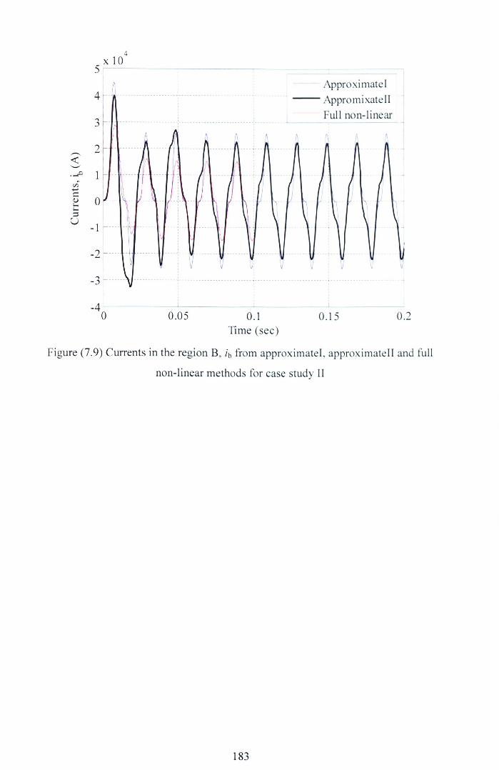
4xlO
5~-----:------~----- _ _L
4 - --------------------------------------- -- ------Approximatel
- -, -- AppromixateIIFull non-linear
_I __,,..,_) - - - -- --- - - -- - ---- - - - - - - - - - - -- -- -- - -- --- - - - - - - -,- - - - ----
- - -- ,:\ '\"
0.05_4L_----~-------------L----o 0.15 0.20.1
Time (sec)
Figure (7.9) Currents in the region B, ib from approximateI, approximateII and full
non-linear methods for case study II
183

Chapter Eight
Unified Electromagnetic Dynamic and
Rotordynamics Model
8.1 Introduction
Procedures for using finite element analysis to approximate magnetic field quantities
in an electrical device are well known ([Arkkio, (1987), Hameyer and Belmans,
(1999), Bastos and Sadowski, (2003)]. To study the mechanical dynamic behaviour of
an electrical machine there is a need for an accurate UMP model (incorporating a
number of current degrees of freedom) and for a high-dimensional rotor dynamics
model. Previous work on the study of coupled (mechanical and electromagnetic)
behaviour of electrical machines have either reduced the electrical behaviour to static
(or very low-dimensional dynamic behaviour) and then focused on the mechanics or
else they have taken very simplistic models of the mechanical behaviour and viewed
the system from the standpoint of the electrical system.
Previous chapters describe how the electromagnetic field equation of an electrical
machine is solved at every time step of the simulation in order to calculate the
inductance matrix of an electrical machine incorporating the material non-linearity. It
also describes how the electromagnetic field equation can be coupled to the circuit
equation to form the electro-magneto-mechanical model. In this chapter a detailed
mechanical model is presented and this detailed model is coupled with a high
dimensional electromagnetic model to study the behaviour of the coupled system.
The combined model coupling electrical and mechanical dynamics facilitates the
following
184

• Voltage is applied to the terminals of the machine and mechanical
speed is taken to be a known input quantity to specify the electrical
problem, and the internal currents are calculated as unknowns.
Parameters of the coupled dynamics are calculated for this set of
internal currents.
• Equations for mechanical motion are coupled to the electrical
dynamics.
The numerical model developed here to study the coupled dynamics of electrical and
mechanical dynamics is generic. In the first application of the model, only cage
induction motors without parallel paths in the stator windings are studied, in the
second application of the model, the effect of parallel winding paths in the system is
incorporated. These parallel paths tend to reduce the net unbalanced magnetic pull by
allowing different amplitude of current to flow in the parallel branches similar to the
effect of rotor cage currents. This model is also used to calculate the equalising
currents in parallel paths.
The chapter is divided mainly into two sections. The first section describes the
proposed combined model coupling electrical and mechanical dynamics. The
electrical dynamics is described by an electro-magneto-mechanical model and this has
already been explained in Chapter 4. A mechanical model of an electric machine is
developed to describe the mechanical dynamics. A coupled model is developed to
describe the combined electrical and mechanical dynamics of an electrical machine.
The second section describes a case study which solves this coupled problem. A 4-
pole three phase induction machine is considered for this study. The machine is
wound in a special way known as the bridge configured windings as described in
Section (4.36) of Chapter 4. Chapter 10 describes the fundamental properties of this
machine presenting the no-load and locked-rotor conditions. The machine has parallel
paths in its stator windings which facilitate to study the effect of the parallel paths in
the machine dynamics. To the knowledge of the author there is as yet no literature
available to include the parallel paths into a rotor dynamic model. One of the
additional features of this coupled model is that it can be easily extended to include
185

the effects of parallel paths. In this section the additional damping offered by the
parallel windings is calculated in terms of energy dissipated in the windings.
8.2 Electro-magneto-mechanical model
The coupled electro-magneto-mechanical model has already been described in
Chapter 5. The linearised coupled equation of this electro-magneto-mechanical model
of an electrical machine is
(8.1)
where {V} is the vector of externally-applied voltages, [R] is the resistance matrix of
the machine including the effect of the end-windings, {IRS } is the vector of
independent currents and {x} is the vector which describe the instantaneous geometry
of the machine. For a two-dimensional analysis {x} comprises only three entries
assuming that neither the rotor nor the stator can deform significantly in the plane and
provided that the stator is fixed in space. The vector, {x} can be written as
(8.2)
where u and v are the horizontal and vertical positions of the rotor centre respectively
and e. is the angle of turn of the rotor. Matrices [A] and [B] are calculated by
differentiating Equation (5.17) and is already explained in Section (5.4) of Chapter 5
how these two matrices can be obtained. For relatively smaller currents, the machine
is not saturated and the matrix [B] is proportional to {IRS}and [pUAHpY) is the
"tangent inductance" or "marginal inductance" matrix. Matrices [B] and [p] [A][pr)are calculated from the magneto-static field equation using 2D FE method.
186

8.3 Mechanical model
The development of mechanical models for rotor-stator-bearing systems is well-
established (Lalanne and Ferraris, 1990) and these models commonly emerge in the
natural second-order form
[MHq} + aD] + n[G ]){q}+ aKmech]+ n[F ]){q}= {f} (8.3)
where [M],[D],[Kmechll denote mass, damping and stiffness matrices of the
mechanical system. Very often, these are all symmetric and positive (semi-jdefinite,
Matrices [F] and [G] are both skew-symmetric and they represent force contributions
from gyroscopic effects and from internal rotor damping respectively. Vectors {q}
and {f} represent the displacements and (externally-applied) forces respectively. With
appropriate definitions for these vectors, {qY{f}represents the instantaneous power
flowing into the mechanical system from the externally applied forces. In fact, the
observations about the symmetry in the matrices above depend fundamentally on this
convention. The mean rotational speed of the rotor is denoted by n in Equation (8.3).
In order to couple the mechanical model to the electromagnetic one, it is necessary to
express the relevant geometry variables of {x} from the previous section in terms of
the displacements in {q}.
{x}= [sf {q}+ [l]"" {x,}+ [l]{x}= [s]' {4}+m=: {x.}+ [~]
(8.4)
(8.5)
where [8] is a selection matrix having three columns. The first two columns of [8]pick out which (linear combinations) of the displacements within {q} constitute the
horizontal and vertical motions of the rotor centre (u and v) respectively. If the
187

mechanical model includes entries in {q} representing rotor twist relative to a frame
of reference rotating at constant speed n, then the third column of [S] contains some
non-zero coefficients. Otherwise, this column contains only zeros. The total force
acting, {f} in Equation (8.3) on the mechanical system is the sum of those
components due to mechanical causes and those due to the electro-magnetic effects
(8.6)
The mechanical force vector, {fM}, is presumed to be known at any instant in time
and it is arises from unbalance and other known sources. In the simulations of interest
here, this vector is zero. In most other cases, it would be a sinusoidal forcing
associated with imbalance and/or bend on the rotor. In the 2D electromagnetic
modelling case where {x} is defined according to Equation (8.2), the electromagnetic
force vector {fE} can have only three independent components - net horizontal force,
U, net vertical force, V, and net (oscillatory component of) torque, Tm and {fE} may
always be written as
{fEl= [S{T~Tm]=:[S{{Xl- [J.]J (8.7)
involving the same matrix [S] that appeared in Equation (8.4) and using Tm to
represent the mean torque exerted by some mechanical load. The product (nTm) is the
useful mechanical power being delivered to that load. The vector {X} is part of the
electromagnetic force vector and contains U and V. This can be obtained in several
different ways. The method favoured here is to draw a closed curve around the rotor
(usually a circle dividing the air gap into a rotor side and a stator side of similar radial
depths) and to integrate force and torque contributions due to Maxwell stresses
(magnetic stresses) around that circle. The method of calculating the force and torque
using Maxwell stresses is explained in Chapter 3. Given the ability to compute {fE}
188

and {fM} at every instant, it is clear that we do have the wherewithal to perform time-
domain simulation of the mechanical system also.
If the magnetic field has been computed at a given instant, t = to, then it is
straightforward to do the integration of Maxwell stresses numerically to obtain
{X}= {Xo}. For small excursions, {xto} from the reference-geometry at this instant,
the time-dependent forcing vector {X} can be approximated well by the linear
expression:
(8.8)
where [KUMP] is usually positive-definite and (because of our definition for {X} as a
force exerted Qy the system rather than on the system) this matrix has a de-stabilising
effect. [KUMP] may be determined by straightforward numerical differentiation in the
magnetic finite-element model at any instant. The matrix [C] represents the influence
of small changes in machine currents on the mechanical system. The quantity
({xtoY[CI{I}-{Io}}) represents the instantaneous marginal power being drawn from
the electrical circuits into the oscillatory mechanical motions. By conservation of
energy, this must be identical to (({I}- {Io}YQP][B]){xto }). It can be concluded that
(8.9)
8.4 Coupled linearised model
In Chapter 5, we outlined the development and format of the electromagnetic model.
This model included the effects of geometry changes and the linearised version of this
model was presented as Equation (8.1) for any instant t= to. Accepting that we have a
reference solution for the machine, it is clear that this linearization of the
electromagnetics is applicable at all times. The linearization includes the effects of
small geometry changes from the expected machine geometry (Le. the reference
solution does recognise the fact that the rotor is rotating).
189

In Section (8.3), the development and format of the mechanical model is outlined. The
purely mechanical aspects of this model were assumed to be linear. The model
included the effects of magnetic forces and the linearization of these forces around the
reference solution was presented as Equation (8.3) for any instant t= to. Note that
{q}=Ofor all times in the reference solution. However since {I} is certainly not zero
in the reference solution, it is convenient for us to define
(8.10)
We deliberately use a vector of charge displacements in place of currents as the basic
time-dependent electrical quantity because of the pleasing structure that it creates in
the time-dependent matrices later. Thus we define
t
{Q~Kt)= f{I~}(T}dT ,o
t
{Qref}(t) = J{Iref KT }dT ,o
t
{Q}(t)= f{I}(T}dTo
(8.11)
Now, this time-dependent linearization of the coupled machine model can be put
together as
The forcing terms on the right hand side of the equation include the mechanical forces
(usually originating from imbalance, rotor bend/misalignment) and slight differences
from the reference voltage. All terms in Equation (8.12) have been defined before
now with the exception of [H]. This matrix represents the sensitivity of the third
column of UpIBD to {I~} and it arises because the vector {x} contains the non-
infinitesimal entry, Cl (c.f. Equations (8.4) and (8.5)). In Equation (8.12), the matrices
which depend on time are [A], [B], [H] and [KUMP].
If the actual coupled response of the machine is of interest, then Equation (8.12)
provides an extremely effective way to obtain that. We caution, however, that as this
190

is a linearised model, it is accurate only for small perturbations from the reference
solution. Transverse deflections at the centre of the rotor should be substantially less
than the radial thickness of the airgap for this analysis to be valid.
Our purposes for the linearised coupled model are two-fold. One interest is the time-
domain response to (small) applied excitation. The other is to do with stability. If the
forcing terms on the right hand side of Equation (8.12) are zero, then Equation (8.12)
represents a homogeneous periodic time-varying linear system.
The period, Tp of any periodic system is defined as the time required repeating the
state of the system. The method of calculating the period of an induction machine is
given later in this chapter. For machines other than induction machines, the period is
much more easily obtained. At any instant, this system has a state which is
characterised by the state-vector
{QJ
{} {q}Y := {Od}
{q}
(8.13)
If there are 2n entries in {y}, then we can discover a (2n x 2n) State-Transition
matrix, [Z] which relates the state at the end of a period, {y}(Tp), to the state at the
start of the period, {yKo), according to
(8.14)
Following the ideas developed by Floquet, the eigenvalues of [Z] show whether the
system is stable. If all eigenvalues are less than 1 in magnitude, the system is stable.
Recall that in the reference solution apIBD is proportional to the magnitude of the
applied voltage - at least for low values of the magnitude of the applied voltage,
{vref }. The negative magnetic stiffness, [KUMP] is proportional to the square of this
applied voltage and the matrix [H] is independent of this applied voltage. At very low
191

levels of applied voltage, the electrical and mechanical dynamics are completely
independent and any instability which might occur will either be purely electrical in
nature (which can occur since many eigenvalues of [H] are negative) or purely
mechanical in nature (which can also occur as a result of internal damping effects
represented by [F]). Other sources of mechanical instability also exist but are not
discussed here.
We study one particular 3-phase induction machine operating in 25 different
conditions - 5 values of slip and 5 different voltage magnitudes.
8.5 The reference electromagnetic solution
Chapter 6 and 7 describe different methods for calculation of the steady state solution
for induction machines. If the rotor is constrained to move concentrically within the
stator and if it is required to rotate at constant mechanical speed n while a fixed-
frequency balanced sinusoidal voltage is applied to the stator windings, then a time-
stepping simulation can be carried out to establish the steady-state machine currents
as a function of time. At this condition if the simulation is carried out by integrating
Equation (8.1) without the final term on the right-hand side the steady state machine
currents is called the reference currents.
For induction machines, this solution depends on both the magnitude of the applied
voltage and its frequency. For reasons that will become clear later, we will invariably
restrict our reference solutions to conditions where the machine rotor has rotated an
integer number of slot-pitches after some periodic time Tp which is also an integer
multiple of the periodic time for the applied voltage waveform. Obtaining this
solution for anyone machine condition can be relatively intensive in computation
time - not least because transients must be allowed to die away before one period of
reference solution is captured and Chapter 7 addresses means for finding this solution.
We have studied the coupled dynamics of the machine for different levels of applied
voltage. A reference solution for a very low applied voltage (say 1V) can obtained
accurately and relatively quickly because the iron behaves linearly and so the element
192

matrices for each finite-element in the model need to be derived only once (in contrast
to the nonlinear case where the matrices must be derived afresh for all ferromagnetic
elements several times per time-step). With magnetic linearity assumed, the reference
currents for an applied voltage of higher magnitude can be scaled - i.e. the reference
solution for 2V is exactly twice the reference solution for 1V. Based on a single
reference solution at low voltage, therefore, we can estimate with confidence at what
voltage it will be necessary to allow for magnetic nonlinearity and moreover, we can
start the simulation for this (slightly non-linear) reference solution with an initial
estimate which will be close to the converged answer. We accept from this point
forward that a reference solution can be obtained for any desired voltage level and any
combination of supply frequency and shaft-speed, n.
8.6 The time period of an electrical machine
For an induction machine with p pole-pairs supplied by electrical frequency, CUe
(rad/s), the so-called "synchronous speed", no (rad/s), is given by
n _CUe0-
p
(8.15)
Synchronous speed is a speed at which the machine develops zero airgap torque. The
time taken for the stator MMF to repeat itself is given by
T = 21rm
(8.16)
If the number of bars in the rotor is k and if the motor is running with a slip of s, thenthe time taken for the rotor to slip one rotor bar is
(8.17)
193

The machine will have perfectly-periodic behaviour if the slip, s, is a rational number,
s = a , {a,b} EN. Then the period, Tp, is given byb
(8.18)
where c is the highest common factor of (Pb) and (lea). For machines other than
induction machines, the period is much more easily obtained.
8.7 Case study of the coupled electrical and mechanics dynamics
of an induction machine
This case study is about the electromechanical interactions of a 2kW induction motor
having flexible rotor. The main electromagnetic parameters of the motor are presented
in Table (8.1). This 4-pole, 3-phase induction motor is wound with a fractional pitch,
double layered bridge configured windings. The stator of an induction machine with
its windings connections and the bridge configured winding scheme are shown in
Figures (4.3) and (4.8) of Section 4 respectively. As mentioned in Chapter 4, bridge
configured windings have six independent currents. Three of them are phase or
terminal currents, denoted by iAph» iBph and iCph, and the other currents are the bridge
or equalising currents, denoted by iAlev, iBlev and iClev, There will be no current flowing
across the bridge for a concentric rotor when the flux field is uniformly distributed.
Any unbalance of field due to eccentricity will induce an EMF tending to drive
currents in the closed circuit such that a MMF comes to exist opposing the rate of
change of this field. Chapters 6 and 7 describe various methods for calculation of
steady state currents of an induction machine for a concentric rotor. To calculate the
equalising currents, which exist because of the rotor eccentricity, the electro-magneto-
mechanical equation is solved by displacing the rotor by a known amount of
eccentricity. The results are presented later in this chapter.
A schematic diagram of the motor is shown in Figure (8.1). The mechanical model of
the motor is developed using mechanical FE software developed by Professor M I
Friswell of the University of Bristol, UK. The rotor and the shaft are modelled using
1D beam elements. The laminations of the rotor are modelled using disc elements.
194

8.7.1 Finite element model of the flexible rotor
Typically the rotor is modelled using around 60 Timoshenko beam elements with four
degrees of freedom per node to represent shaft stiffness and using rigid disc elements
fixed at the appropriate shaft-stations to represent the additional mass of blade-stages
(in the case of turbo-machines) or (in the case of electrical machines) the laminated
core of the rotor. Each node of the model has two translational degrees of freedom
and two rotational degrees of freedom. In some cases, (Garvey, et al., 2004), it is
critical to take account of the stiffening effects of the laminated rotor core on the
shaft. Figure (8.2) shows a typical finite element model of an induction machine
where the shaft is supported by two preloaded angular contact ball bearings at each
end. The bearings are assumed to be isotropic and they are represented using
equivalent stiffness and damping properties. The equivalent stiffness and damping
properties of the bearings are shown in Table (8.2). Figures (8.3) and (8.4) show the
system Campbell diagram and the mode-shapes associated with the first four
(forward-whirling) critical speeds. These forward critical speeds occur at 3843, 8939,
15000 and 20040 rpm
8.7.2 Equalising currents for an eccentric rotor
An eccentric rotor creates an asymmetric flux distribution that causes the radial
forces. The asymmetric field may induce circulating currents in the rotor cage and
parallel paths of the stator winding. These currents tend to equalise the flux
distribution and they may significantly reduce the amplitudes of these radial forces.
Therefore, from the electrical dynamics alone we can measure the equalising currents
for an eccentric rotor. In other words, these equalising currents are the measures of
eccentricity of a particular machine at its operating conditions.
Numerical tests (linear) are carried out at 20V supply voltage with varying degree of
static eccentricity. Figures (8.5), (8.6) and (8.7) show the levitation currents in the
three bridges because of the static eccentricity of 2% of the air gap, which are
otherwise 'zero' for a concentric rotor. Similarly, Figures (8.8), (8.9) and (8.10) show
the levitation or equalising currents in the three bridges based on the 10% static
195

eccentricity in the airgap. The magnitudes of the equalising currents are 4% of the
phase currents when the static eccentricity is 2% of the airgap. It can be seen from
these figures that the equalising currents vary linearly with the eccentricity.
8.7.3 Minimum time period of the machine
The minimum time period of the induction machine is calculated using Equation
(8.18) For example, if the supply frequency if> is 25 Hz, the number of rotor bars (k)
is 32 of a 4-pole induction machine, then the minimum time period is calculated as
follows:
The time taken for the stator MMF to repeat itself, Tm = _!_ = 0.04 secf
For a slip of 2.5% the time taken for the rotor to slip one rotor bar, Thar =]!_ Tm = 0.1ks
sec. For slip 2.5%, a = 25 and b = 1000. The highest common factor, c of (Ph) and
(lea) in this case is 400 and the period of the machine is
Tp = ph Tm = 5 x 0.04 = 0.2 secc
8.7.4 Preparing the state transition matrix for the coupled model
To determine the system characteristics, we are interested in solutions for Equation
(8.12) where forcing term, {f}, is zero for all time. We can write Equation (8.12) as
[M'(t)] {q'(t)} + [D'(t)] {q'(t)} + [K'(t)] {q'(t)} = 0 (8.19)
We can write Equation (8.19) in state-space form
[\(t) -~'(t)I::~:lJ+[~Y~M~(tl::~:lJ= [~]
=: [A{t )Hx{t )}+ [B{t )Hx{t )}
(8.20)
196

The time-varying coefficient matrices of the linearised coupled dynamic equation are
periodic. The Floquet method is used to analyse the stability of this linear time
varying periodic system. The state vector, {x{t)}, has 2n entries in it. Given any initial
vector, {x{O)}, it is straightforward to integrate Equation (8.20) numerically through
one time-period, Tsys, to develop {x{I:ys)}. In fact, the fastest method for achieving this
would take account of the second-order nature of the system. We apply Newmark-
Beta (Newmark, 1959) algorithm for numerical integration. By generating 2n linearly-
independent initial state vectors {x(O)} and integrating each one through one complete
period, we can develop a so-called State Transition Matrix (STM), [Z], such that
given any arbitrary initial state vector, {x{O)}, the state-vector at the end of the period
is given by
{x{TsyJ}= [Z]{x{O)} (8.21)
8.7.5 Stability of the system
The stability of the linear system with time varying coefficients is analysed using the
Floquet method. The eigenvalues of the STM are calculated for different slip
conditions and different voltages at the end of one period and that determines the
stability of the system. Table (8.4) shows the stability condition of the system for
different slips and supply voltages. It is found that the system is stable for all slip
conditions at 22.5 V and unstable for 51 V or above. At 25.5 V the system is stable at
2% of slip or less and unstable beyond 2%. At 34 V the system is stable at 0.5% of
slip or less and unstable beyond 0.5%. It is also possible to draw a stability chart with
slip versus the supplied voltage.
8.7.6 Energy transfer while closing the bridge
The one of the main points of interest of this study is the effective mechanical
damping provided by the closure of the parallel-path circuits in the three different
phases. The parallel paths do not stabilise any of the unstable conditions (which
197

appear to be dominated by negative magnetic stiffness) but they do reduce the real
parts of eigenvalues in all cases. Effective electrical damping has been assessed by
forcing the rotor centre to take a positive circular synchronous orbit of 1% of the air-
gap and examining the energy transferred into the electrical circuits from the
mechanical motion over the period of time, Tp. Tables (8.5) and (8.6) summarise the
findings at 17V for each of the five conditions of slip with the parallel paths closed for
forward whirling and backward whirling of the rotor respectively. These results are
presented as time-constants (the mean total mechanical energy in the rotor divided by
the mean power-loss into the electrical system).
Energy transferred to the electrical system from the mechanical system because of the
displacement of the rotor from the central position as a function of time is shown in
Figures (8.11) and (8.12) for forward and backward whirl respectively. As expected
the energy transfer is greater when the rotor is in forward whirl than it is in backward
whirl.
8.8 Conclusions
A coupled model combining the electrical and mechanical dynamics is proposed. The
results of this coupled model are verified by experimental results and this is explained
later in Chapter 10. The coupled system is a time varying linear system with periodic
coefficients. A method for analysing stability of time varying periodic system is also
described.
198

Rotor Shaft
Figure (8.1): Schematic diagram of an induction machine
----------------------------------~~
Bearing 2
~
Table (8.1): Main electromagnetic parameters of the machine
Parameters ValueNumber of polesNumber of phase
Number of stator slotsOuter diameter of the stator [mm]Inner diameter of the stator [mm]
Number of rotor slotsOuter diameter of the rotor [mm]
Air gap radial thickness [mm]Length of the rotor [mm]
Rated voltage [V]Rated frequency [Hz]
Rated power rkW]
4336153933292.20.4123415502
199

Figure (8.2): Finite element model of the induction machine
Table (8.2): Coefficients of the bearing
Stiffness (in N/mL) Damping (in N/mL)
kxx kxy kyy kyx Cxx cxy Cyy cyx
Brg.#l 5.0 e7 0.0 5.0 e7 0.0 0.0 0.0 0.0 0.0
Brg. #2 5.0 e7 0.0 5.0 e7 0.0 0.0 0.0 0.0 0.0
200

350~------~----~------~------~~-~------------~==========~----~~-~
>. Is»
~ 200~<l)....~
0.5 1 1.5 2Rotor Speed (rpm)
Figure (8.3): Natural speed versus rotor speed
4xlO
First Critical Second Critical
Third Critical Fourth Critical
Figure (8.4): First four modes of the system
201

6~----~------~--~--~----~-------:1
:1- -- --~-- -- -- - -- ---
~ --- -----
4 --------------- ----- ------ ,---
2 --------- -- --- -~--- +~--- ----- ----- - ---- - -----
$ 0 ---~~---- -- --- -- --- ------J --_If - l~------------ If
j ::"•••.~•••....••.~...~.•••••••••••••-6 -----------------~-----------------~-------------
_sL_----~------~------L-----~------~o 0.2 0.4 0.6 O.STIme (sec)
Figure (8.5): Equalising current per meter of axial length in phase A bridge for an
eccentricity of 2% of the air gap and when supply frequency is 25 Hz and slip is 2%
6~----~------~----~:------~:----~
2 e f f·.· ~Ii ~.. .:2 0 ·····lJ··" LIH~\' . . .i .2' .., ~.,L t ,.~.II.l~.8 :: ••·~l~·.1.·.··•••1.1.
\ : :. , ., , , ,-s - ------------c- --- ----- -- -- ----r------- --- ------ -,-------- -- -- ----- r- --------------i :-10~----~------~------L-----~----~o 0.2 0.4 0.6 O.S
----- --. ------4~---------------+---------------
TIme (sec)
Figure (8.6): Equalising current per meter of axial length in phase B bridge for an
eccentricity of 2% of the air gap and when supply frequency is 25 Hz and slip is 2%
202

:~ l .4 : .
_8L-----_L------J_------L_----~------~o 0.2 0.4 0.6 0.8TIme (sec)
Figure (8.7): Equalising current per meter of axial length in phase C bridge for an
eccentricity of 2% of the air gap and when supply frequency is 25 Hz and slip is 2%
30~----~------~------~----~------~
20 > •••••••••••••
10 . . . "1 .~ 0 ..~.. .. .\/l ji'l .e ~ 1\ II8 -Io~l···· . , ~ .-20 ..---: H··· .. ..
, ,-30 ~·· ·· ..r·· · ~·· ··.... .. ; -
, ,
_40L-----_L------J_------L_----~------~o 0.2 0.4 0.6 0.8
TIme (sec)
Figure (8.8): Equalising current per meter of axial length in phase A bridge for an
eccentricity of 10% of the air gap and when supply frequency is 25 Hz and slip is 2%
203
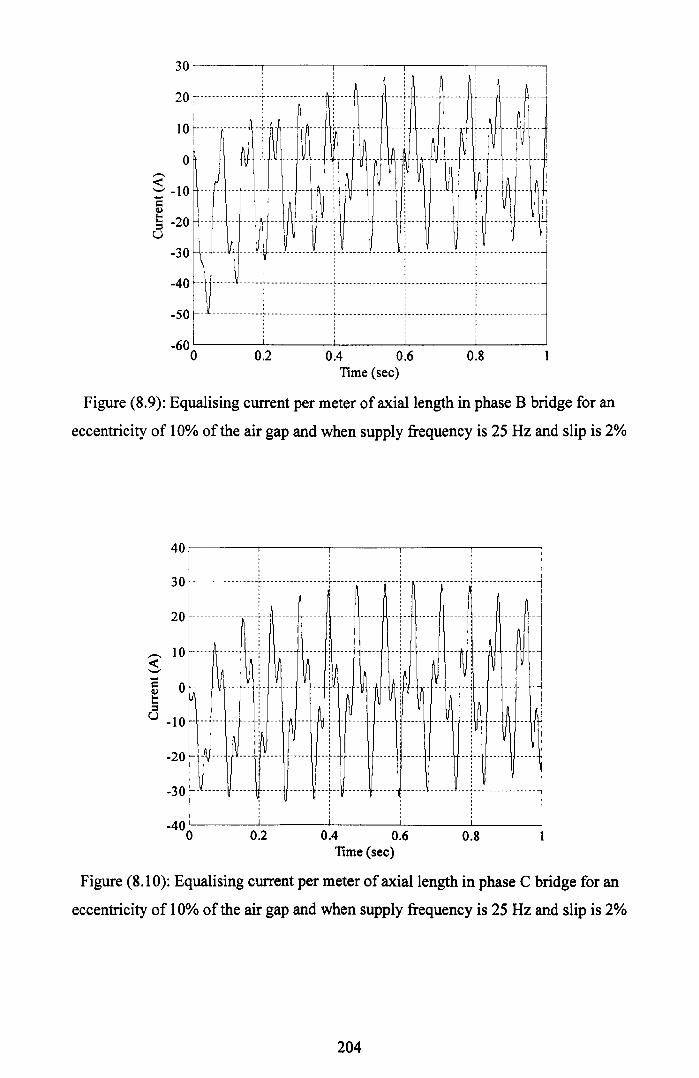
30~--~----~-----:~--~-----'20 -----------------~---------------
lO ············'~llli.....LN I 1\+_ 0 ---N -J~---_V_ ----~' --- (f- -l :-tr-~- --- -- --- -- --- --i-IOJ ...··f ...~.....~ltll iJ' ·l·11 ...~8 ::: ••·.••.~·.•••~..••....•••..•••L· •••..•••••.r••..••••..••..:•.•.••••..•••••.
-40~- ------------t-----------------t-----------------i-----------------i----------------, , ,
-50 r-- -------------t-----------------(--------------f-----------------i-----------------, ,
Time (sec)
-60~----~------~------~----~------~o 0.2 0.4 0.6 0.8
Figure (8.9): Equalising current per meter of axial length in phase B bridge for an
eccentricity of 10% of the air gap and when supply frequency is 25 Hz and slip is 2%
40~----~------~------~----~------~
30 ----------------~-----------------~-------------
20 ----------------+-- ------ ------ ----- ------
$ 10 . VC ( ;.. . :~··I\·! o,~ .. >.-J~ --- ~~-,ii,;-u -10 --~, '--n - M --.------ -__LjU' ---~ -..
-20 Nt :'--.--.-L-- - '-,- -.--'-30 - ------ ------ ----- ------ ---"-- ------ ----- ------ ------ ---.----------------
_40L-----~------~------~----~------~o 02 OA O~Time (sec)
0.8
Figure (8.10): Equalising current per meter of axial length in phase C bridge for an
eccentricity of 10% of the air gap and when supply frequency is 25 Hz and slip is 2%
204

Table (8.3): The minimum periods of a machine with parameters given in Table (8.1)
for different slips
Slip(%) Period of the system (s)
0.5 1.00
1.0 1.00
1.5 1.00
2.0 1.00
2.5 0.20
3.0 1.00
4.0 1.00
5.0 0.20
Table (8.4): Stability chart of the machine at different slips for different voltage levels
Supply Stability of the machine at different slips for different voltage levels
Voltage Slip = Slip= 0.5% Slip = 1% Slip= 2 % Slip =2.5% Slip = 5.0%
(V) 0 Period = Is Period = Period = Period = Period =
Is Is 0.2s 0.2s
17.0 ...j ...j ...j ...j ...j ...j
20.4 ...j ...j ...j ...j ...j ...j
22.1 ...j ...j ...j ...j ...j ...j
25.5 ...j ...j ...j ...j X X
34.0 ...j ...j X X X X
51.0 X X X X X X
205

Table (8.5): Time constants with the parallel paths closed for five different slips in
case of forward whirling
Supply Time constants (s)
Voltage Slip = 0 Slip = 0.5% Slip = 1% Slip = 2 % Slip = 5%
(period= 1s) (period= 1s) (Period= 1s) (Period= 1s)
17V 0.00187160 0.00173507 0.00146956 0.00117471 0.00157921
34V 4.6790e- 4.3377e-004 3.673ge-004 2.9368e-004 3.9480e-004
004
Table (8.6): Time constants with the parallel paths closed for five different slips in
case of backward whirling
Supply Time constants (s)
Voltage Slip = 0 Slip =0.5% Slip = 1% Slip =2 % Slip = 5%
(period= 1s) (period= 1s) (period= 1s) (period= 1s)
17V 0.39781394 0.37390752 0.29176840 0.20925626 0.15278131
34V 0.09945348 0.09347688 0.07294210 0.05231406 0.03819532
206

-6 c ---- -------------
-1 -
-2 c~-.'-'....Q)~ -3 ------------------,------------------!.------c 'C'O....;:0 -4 -------------------- -- 0.000....~ -- 0.005t.D
-5 ----- --------- --0.010
--0.020
-- 0025
-- 0_050-7~~~~~~~~~~~~~~~~~~~~~2.5 3 3.5 4 4.5 5
Time (sec)
Figure (8.11): Energy transfer to the electrical system from the mechanical motion
due to forward whirling for different slips
-0.045 L
, ,- - - - - - - - - - ... - - - - - - - - - - - - - - - - -~- - - - - - - - - - - - - - --, ,-0.005 -
-001 ~-------
I2 -0.0151-------------:-----
,2 -0.02 ~--------------:------~ I I~ -0;::r .•......... I=O~OO ...~ -0 035 ~ -- 0.005 --------------_
. -- 0.010
-0_04 ~--------------- -- 0_020
4 4.5 5Time (sec)
Figure (8.12): Energy transfer to the electrical system from the mechanical motion
due to backward whirling for different slips
207

Chapter Nine
Methods for Reducing Unbalanced Magnetic Pull
9.1 Introduction
Several people have studied UMP due to eccentricity and most notably Belmans et al.
(1984), Kovacs (1977) and Frunchtenicht (1982) but very few people has
recommended methods for reducing UMP. Among these are Bradford (1968), Krondl
(1956) and Dorrell and Smith (1994). Bradford's (1968) experimental machine
consists of a 6-pole series connected type which could be used in conjunction with a
blank, wound and a cage rotor. He concluded that because of its parallel paths cage
rotor damped the UMP much higher degree than blank and wound rotors. Krondl
(1956) and Dorrell and Smith (1994) concluded that parallel stator windings damp
UMP which in turn reduces the motor noise and vibrations.
A generic method for reducing UMP using secondary windings in the stator of an
electrical machine was put forward by Kozisek (1935), Garvey and Watson (2004).
One drawback of these methods is that it occupies some space in the stator slots which
otherwise could have been used for torque production. The effectiveness can be
increased by increasing the total cross sectional area of the secondary coils but at a
sacrifice of main windings.
One passive method for reducing the UMP in an electrical machine is discussed here
and its effectiveness is verified with an experimental setup in Chapter 10. The method
uses the main torque producing winding to suppress the UMP due to eccentricity. In
this chapter the working principles of this method is discussed.
208

9.2 Reduction of UMP in an induction machine using bridge
windings
The bridge configured windings, first introduced by Khoo (2005), overcomes the
drawback of secondary windings proposed by Garvey and Watson (2004). This
unique scheme has three-phase terminals for torque production and additional
terminals for active or passive magnetic bearing action control. Active control can be
deployed by connecting the terminals devoted to lateral forces to closed-loop
controllable current or voltage sources. Passive control of UMP can be accomplished
by short circuiting the additional pairs of terminals or "closing the bridge". In this
work only the passive control of UMP feature of this bridge winding is introduced.
Both torque-producing and induced currents flow in the same set of conductors in the
bridge configured winding scheme. A detailed explanation about the bridge
configured winding can be found in (Khoo, 2005).
Figure (9.1) depicts a three-phase induction motor having distributed coils wound on a
36-tooth stator. Coil groups "ai-as-a," and "aa-a--a," are wound and aligned at the
same axis of symmetry. Likewise, coil group "aaj-aai-aa," and "aaa-aae-aa," are
wound at the diametrically opposite tooth and their terminals are connected to coil
group "al-a2-a3" and "aa-ae-a," to form a bridge. Coils in phases "B" and "C" are
connected in a similar manner.
No current will flow across the bridge if the rotor is concentric and the stator MMF is
symmetric (flux field is uniformly distributed) i.e. bridges iAlev, iBlev and iClev are zero.
Any unbalance of field due to eccentricity will induce an EMF tending to drive
currents in the closed circuit such that a MMF comes to exist opposing the rate of
change of this field. The currents flowing across the bridge are known as equalising
currents. The feature which makes the bridge winding different from the other passive
methods for reducing UMP is its provision for active control. When the bridge is
connected to a controllable power supply with feedback control, the rotordynamic
behaviour of the machine can be controlled. Additional currents required to bring the
rotor to the centre will be provided by the controllable power supply. With proper
control strategy the response of a flexible system at critical speeds can be subdued
209

dramatically by using this controlled UMP within the electrical machine (Khoo, et al.,
2004).
9.3 Conclusions
One method of passive control of UMP of an electrical machine is discussed. Though
only the passive feature of bridge configured winding is studied in this study, the
machine with the bridge configured windings can be used for active control of UMP.
The bridge configured winding possess many interesting features which are beyond
the scope of this study. Some of them are explained in (Khoo, et al., 2004) and (Khoo,
et al., 2005). For secondary windings to be effective in reducing the UMP one must
increase the number of turns of the secondary windings and this call for extra space in
the stator slot. For the same performance the machine with the bridge configured
windings will be smaller in size and weight than those with secondary windings.
210

Figure (9.1): Stator of an electrical machine showing the winding connection. Red,
blue and yellow colours show the three different phases.
aa,
iCph
Figure (9.2): 4-pole, 3-phase induction motor with a bridge configured windings
211

Chapter Ten
Experimental Validation
Chapter 5 describes the modelling of an electro-magneto-mechanical device and
describes the coupling of circuit equation and field equation of an electrical machine.
Chapter 6 describes different methods of calculating steady state characteristics of an
induction machine using linear as well non-linear FEA. Chapter 7 describes a
numerical model which unifies electromagnetic and mechanical dynamics. Using this
numerical model Chapter 8 also analyses the stability of a 4-pole, 3 phase 2 kW
induction motor. Chapter 9 describes the method of reducing UMP using equalising
connections.
10.1 Introduction
Often experiments are required for accurate determination of machine parameters.
Some physical phenomena are difficult to model accurately and experiments are also
required for clear understanding of these phenomena. An experimental setup has been
commissioned to investigate the electromechanical interactions of an induction
machine. The parameters of the machine are chosen to be the same as the machine for
the case study in Chapter 8. The motor is wound as a 3 phase, 4-pole bridge
configured windings, which as explained in Chapter 9. The aims of this experimental
study can be summarised as follows:
• Verify the results of the coupled model (numerical) combining the electrical
and mechanical dynamics proposed in Chapter 8.
• Investigate the effectiveness of the bridge configured windings as a passive
method for reducing UMP.
In this chapter, the experimental procedures to investigate the electromechanical
interaction of an induction machine are described. Experimental results are presented
212

and compared with the numerical results. The effects of equalising connections
produced by bridge configured windings in reducing UMP are clearly demonstrated.
10.2 Design of the test rig
The design of the test rig is divided into two categories: electrical and mechanical
design. They are discussed in the following sections.
10.2.1 Motor electrical design
The electrical motor is a 4-pole induction motor with 2 kW capacity. The main
electromagnetic parameters of the machine are given in Table (8.1) of Chapter 8.
10.2.1.1 Winding scheme
The main torque-producing stator winding is connected according to the bridge
configured winding scheme [Khoo, et al. (2002). Khoo, et al. (2005)], forming a four-
pole motor configuration. The bridge configured winding is a unique scheme and it
has three-phase terminals for torque production and additional terminals for active or
passive bearing action control. The winding scheme of the machine in the
experimental rig is a 4-pole, 3-phase double layered fractional pitch windings. Figure
(8.1) depicts a three-phase induction motor having distributed coils wound on a 36-
tooth stator. Coil group "ai-aj-a," are connected in series with coil group "Wi4-aa5-a~"
and this coil group in turn is connected in parallel with series group "aai-aar-aa," and
"~-a5-~". Coils in phases "B" and "C" are connected in a similar manner. Details
about the passive control of UMP using this winding scheme can be found in Chapter
9.
10.2.1.2 Full pitch and fractional pitch
The pole pitch is the angular distance between two adjacent poles on a machine. The
pole pitch of a machine in mechanical degrees is
213

(10.1)
where Pp is the pole pitch in mechanical degrees and p is the number of pole pairs of
the machine. Regardless of the number of poles on the machine, one pole pitch is
always 180 electrical degrees. If the stator coil stretches across the same angle as the
pole pitch, it is called a full-pitch coil. If the stator coil stretches across an angle
smaller than a pole pitch, it is called a fractional-pitch coil. The pitch of a fractional-
pitch coil is expressed as a fraction indicating the portion of the pole pitch it spans.
There are good reasons for using fractional-pitch windings (Chapman, 1998). These
concern the effect of the non-sinusoidal flux density distribution in real machines. The
MMF produced by the coils is not sinusoidal and it contains many harmonics. When
the voltage waveform is symmetric about the centre, no even harmonics are present in
the phase voltage. However, all the odd harmonics (third, fifth, seventh, ninth, etc) are
present in the phase voltage to some extent and need to be dealt with the machines.
Table (10.1) shows the harmonics for full pitch and fractional pitch of the voltage
waveform. In the test rig we have chosen the fractional-~ because amongst the cases9
shown in the table it has the lowest proportion of the third harmonic. The fractional-
pitch reduces the magnitude of the output voltage slightly, but at the same time
attenuates the harmonics components. Figure (10.2) shows the MMF harmonics with
fractional pitch - ~ of the stator windings.9
10.2.1.3 Number of turns in each coil
In this subsection the calculation used in designing the machine winding is described.
The number of turns per coil is calculated for the winding scheme proposed in the
experimental rig based on the total flux density of 1 Tesla in the airgap. We assume
that the MMF distribution is sinusoidal. First the individual fluxes for the three coils
ai, a2 and a3 are calculated.
+(7~6)Coil ai has flux, <1>1 = rlBmax J cos{2B}dB = rlBmax Wb
_(11~6)
214

where I is the axial length of the machine, r is radius of the rotor and Bmax is the
maximum flux density.
+(%)Coil a2 has flux, <1>2= rlBmax J cos{2ti)do = 0.939 rlBmax Wh
-(%)
+(11Y3'6)Coil a, has flux, <1>3=rlBmax J cos(20)do = 0.939 rlBmax Wh
_(7Y3'6)
Total flux, <I> = 2.878 rlBmax Wb. For a rotor of length, l= 123 mm and radius, r = 46
mm and Bmax~ 1.0 Tesla, the total flux, <I> is 16 x 10-3Wb.
In the case of bridge configured windings three full coils, ai, a2, and a3 together forms
a coil group as shown in Figure (8.2) of Chapter 8. There are four coil groups per
phase. Since there are four coil groups per phase and the total voltage, Emaxin one
phase in which the coils each carry N turns is
Emax = 4<l>{2tif)N (10.2)
where/is the supply frequency. From Equation (10.2) we get
N- Emax- 4<l>{2tif)
(10.3)
Using the above calculated values for <I> and considering the values for Emu and
supply frequency is 415 V and 50 Hz respectively, the value of N is found to be 17.
10.2.2 Drive system for the motor and electrical sensors
10.2.2.1 Drive system for the motor
A frequency converter is the best way to control the speed of an induction machine.
The most common frequency converter type is the voltage-source converter with
pulse width modulation (PWM). The frequency converter used to control the
215

induction used is manufactured by ABB (ACS140) and has a power ratings of up to
2.2 kW. The motor voltage consists of rectangular pulses with a switching frequency
as high as (3-20 kHz). The currents are nearly sinusoidal since the motor is inductive
and the very high frequency components associated with carrier frequency and
multiples of that are fairly effectively filtered out.
10.2.2.2 Current transducers
Hall effect closed loop (compensated) multi-range current transducers (LTS 15NP)
are used to measure the currents. These current transducers can measure DC, AC,
pulsed currents and equipped with a galvanic isolation between the primary circuit
(high power) and the secondary circuit (electronic circuit). Because of its compact
design it can be easily mounted on a PCB. This current transducer has an extended
measuring range. In the present case, we set the range at -15 to +15A. The measuring
currents have a linear relation with the output voltage with linearity < 0.1%. The
current transducers were calibrated to measure between -5.5 to +5.5 A. The output
voltage is fed to a data acquisition system for further processing.
10.2.2.3 Voltage transducers
Hall effect Closed loop (compensated) voltage transducers (L V 25NP) are used to
measure the voltages. This voltage transducer can measure DC, AC, pulsed voltages
and equipped with a galvanic isolation between the primary circuit (high power) and
the secondary circuit (electronic circuit). The measuring range is configurable. We
have set the range at -100 to +100 V. The measured voltage has a linear relation with
the output voltage with linearity < 0.2%. The voltage transducers were calibrated to
measure between -74 to +74 V. The output voltage is fed to a data acquisition for
further processing.
10.2.3 Mechanical design of the system
For an eccentric rotor a significant UMP force is produced in the airgap usually
tending to pull the rotor even further away from the concentric position. Thus for a
216

stable operation the mechanical stiffness of the shaft must be greater than the negative
stiffness introduced by the UMP.
The mean airgap for the induction machine used in this experimental rig is 0.4 mm.
The negative stiffness is the slope of the curve of magnetic force in the airgap versus
displacement of the rotor. Magnetic forces are calculated by solving the magnetic
field when the rotor is shifted from centre along positive x-direction as well as
negative x-direction. Figure (3.17) of Chapter 3 shows the magnetic forces per unit of
axial length versus eccentricity of the rotor when 3-phase currents with a peak of 200
A (per slot) is applied. The slope of this curve is 2x 10⁶ N/m per meter of the axial
length. From this negative stiffness the total load is calculated for a travel of the
airgap and this is ~ 800 N. The shaft is designed for up to a loading capacity of 1000
N. This force is regarded as a concentrated load on a simply supported beam. The
diameter of the shaft is calculated based on the assumption that the deflection of the
beam in the motor position is 30% of the airgap. Figure (l0.3) shows a simply
supported beam with a concentrated load. The deflection of the beam under the load is
8 =Wa2(I-aYw 3EIl
(10.4)
where W is the concentrated load, RI and R2 are the reaction forces, a is the distance
ofW from reaction force, RI, I is the length of the beam. In our case: W= 1000N, a =156.5mm, and I = 1020 mm. It is found that for a 50 mm diameter shaft the deflection
under the load is nearly equal to 25% of the airgap. Thus a shaft with diameter of 50
mm is chosen for the rig.
10.2.4 Other transducers
The impact hammer method is a convenient and economical excitation method for
injecting known inputs into a vibrating system. The impact hammer consists of a
hammer with a piezoelectric force transducer at its tip. The impact hammer is highly
portable for fieldwork and provides no unwanted mass loading to the structure under
test. The impact hammer produces an impulse force at one hit, which excites the
217

structure with a constant force over a frequency range of interest. The waveform
produced by an impact hammer is an impulse. The test setup for impact hammer
excitation experimental is shown in Figure (l0.4). An impact hammer with an output
ofO.01 Volts/g is used to supply an impulse force signal. A signal conditioner is used
for conditioning the input force signal. The input signal is measured using a multi-
channel signal analyser.
Aluminium foil strain gauges are mounted in the bearing housing at one end of the
shaft. Figure (lO.S) shows the strain gauges along with the bearing in the rig. Figures
(10.6) and (10.7) show the strain gauge calibration curves for forces along x and y
directions. The test setup is shown in Figure (10.1). Horizontal and vertical forces are
measured separately and fed into the oscilloscope. The vertical force signal is
measured using a multi-channel signal analyser.
10.2.5 Data acquisition
The sensor or transducer signals are often incompatible with the data acquisition
interface and these signals must be conditioned before they are fed to a data
acquisition interface. The analog signals are converted to digital signals via the analog
to digital converter of the data acquisition interface. The data acquisition card used is
a dSPACE DS1104 R&D Controller Board. The whole unit is used in conjunction
with Matlab, Simulink and Real time workshop software package. The data
acquisition card has 8-channels where 4 multiplexed channels equipped with one
sample and hold AID converters, another 4 parallel channels each equipped with one
sample and hold converters.
10.3 Numerical model verification with experimental results
Figure (10.8) shows a schematic diagram of the experimental rig. The rig consists ofa
4-pole 2 kW induction motor with a long and flexible shaft. This motor is wound with
fractional pitch double-layered bridge-configured windings. The stator of the machine
with the winding connections and the bridge configured winding scheme are shown in
Figures (4.2) and (4.7) of Section 4 respectively. The shaft is supported by preloaded
218

angular contact ball bearings at each end. This whole assembly is fixed on the top of a
steel plate. Strain gauges are mounted in the bearing #1 which is situated in the left
hand side of the shaft. The right end of the shaft is attached to another shaft via a
flexible bellows coupling and this second shaft is coupled to another induction motor
via a belt drive. The second induction motor is used as a brake by applying DC
currents across the terminals (plug braking). This section compares the results from
the numerical model with that of experiments.
10.3.1 Mechanical model
The development of the mechanical model can be found in Section (7.3) of Chapter 7.
We can write the equation of motion of the mechanical model as
(10.5)
where UM], [D],[Kn denote mass, damping and stiffness matrices. The mean
rotational speed of the rotor is denoted by n.
In Chapter 8 we have solved the mechanical model numerically using FEM without
considering the effect of the base plate.
Tests using an impact hammer test are used to investigate the mode shapes of the rig.
The experimental setup for the impact hammer test is shown in Figure (10.8). The
hammer produces an impulse force at a single hit and this excites the structure with a
fairly flat force spectrum over a given range of frequency. The response signals are
captured with the strain gauges and these signals are amplified and conveyed to a
signal analyser. We have chosen 12 locations for excitation on the rig i.e. 5 points on
the shaft and 7 points on the base plate. The frequency range is selected as 0-160 Hz.
Frequency response functions were obtained taking 16 averages at each location in
order to reduce the effects of the noise. The shaft was rotating while the FRFs were
being obtained. We get a total of 12 FRFs. Figure (10.10) shows a FRF at when the
impulse is applied at point 3 on the shaft. Mode shapes can be calculated once the
FRF at 12points is obtained by solving the following equation
219

(10.6)
where htj (m) is one entry of the frequency response matrix, Akk is the k-th eigenvalue,
m is the excitation frequency, 'L,ik represents the amount by which one unit of
excitation at input degree of freedom #j excites mode #k and 'R ik: represents the
amount of output at output degree of freedom #i is contributed by each mode #k. The
derivation of frequency response matrix for a second order system is explained in
Appendix B.
Figures (10.11), (10.12), (10.13) and (10.14) show the modes shapes of the rig at 1.35
Hz, 58.61 Hz, 65.78 Hz and 72.39 Hz respectively. The deflected and un-deflected
rotor and base are shown separately and they are distinguished by different colours.
Mode shapes obtained from the numerical model are shown in Chapter 8. Since the
effect of the base plate is not considered in the numerical model explained in Chapter
8, therefore there is a slight difference in the results. The numerical model can be
improved by incorporating the effect of the base plate.
10.3.2 Electrical model
The development of electrical dynamics coupling circuit equation with the field
equation is explained in Chapter 5. For a constant mechanical speed, nmech the
electro-magneto-mechanical equation can be written as
(10.7)
where {V} is the vector of externally-applied voltages, [R] is the resistance matrix of
the machine including the effects of the end-windings, {IRS} is the vector of
independent machine currents, 0 is the angular position of the rotor and
[Lmar{{IRs},B)] is the marginal inductance matrix which is a function of machine
220

currents and angular position of the rotor. Chapter 6 discusses different methods of
calculating marginal inductance of an induction machine. The results of this
numerical model are compared with the experimental results of a rig with the same
parameters.
To solve the numerical model, the circuit equation [Equation (l0.7)] is solved for no-
load and locked-rotor conditions using ode45 integration routine of MATLAB.
Marginal inductance [Lmar({IRs},B)]is calculated by solving the field equation using
MagFEA, the 2D FEA code developed in the MATLAB environment. Material non-
linearity is not considered for this calculation. End winding effects are also not
included in the resistance and inductance matrix. The applied voltages at the stator
windings terminals are:
V A = Vmcos(rot)
VB =Vmco{ mt_2;)
Vc = VmCOs( rot _ 4;)(10.8)
The stator and rotor currents are obtained for no-load and locked-rotor conditions for
Vm= 1 V. These numerical results are compared with the experimental results by
scaling the stator and rotor currents according to the voltage obtained from
experiments.
The supply voltage and stator terminal currents of the experimental rig are measured
using voltage transducers and current transducers respectively for no-load and locked-
rotor conditions. The following section compares the experimental results with the
numerical results.
10.3.2.1 No-load test
The no-load test of an induction motor measures the rotational losses of the motor and
provides information about its magnetization current. The only load on the motor is
221

the friction and windage losses. Experiments are carried out for the noload test by
spinning the rotor at synchronous speed for different supply frequencies. The supply
frequencies are chosen as 20, 25, 30, 35, 40, 45, and 50 Hz. Figures (10.15) and
(10.16) show the no-load supply voltages and stator phase currents from numerical
model as well as from the experiments when the supply frequency is 20 Hz. The
experimental results show a very good agreement with the numerical results. Figures
(10.17) and (10.18) show the no-load supply voltages and stator phase currents from
both numerical model and experiments when supply frequency is 25 Hz.
10.3.2.2 Locked rotor test
When voltage is applied to the stator windings of an induction motor, EMFs are
induced in the rotor circuits of the machine. Generally, the greater the relative motion
between the rotor and the stator magnetic fields, the greater the resulting rotor EMFs
and rotor frequency. The largest relative motion occurs when the rotor is stationary
and this situation is called the locked-rotor or blocked rotor condition, so the largest
voltage and rotor frequency are induced in the rotor at that condition. A voltage is
then applied to the motor and the resulting voltages and currents are measured with
the help of voltage and current transducers respectively. Figures (10.19) and (10.20)
show the locked-rotor supply voltages and stator phase currents from numerical model
as well as from the experiments. The machine is saturated in the locked-rotor test. As
mentioned earlier magnetic saturation is not considered in the numerical model,
therefore currents from the experiments are higher than the numerical one.
10.4 Results for the modified motor
As mentioned in Section (10.2.1.1), the induction machine under test is wound with
bridge configured windings. This unique winding scheme can be used for torque
generation as well as for passive or active modification of UMP. The arrangement of
the bridge configured windings shown in Figure (9.2) has two parallel paths with one
equalising connection in each phase. Because of the inevitable manufacturing and
assembling tolerances, there will be always, to some degree, a non-uniform airgap in
an electrical machine. This problem is particularly significant for small and medium
222

sized induction machines with a nominal airgap of a fraction of 1 mm (Ellison et al.,
1971). We expect some degree of non-uniform airgap in our machine.
If the rotor happens to be concentric and if the stator is electromagnetically
symmetric, there will be no equalising currents even if the equalising links are short
circuited. In case of an eccentric rotor obviously there will be no net equalising
currents flowing when the equalising links are not short circuited. Once the equalising
links have been short circuited, any unbalance of field present will induce an EMF
tending to drive currents in the closed circuit such that a MMF comes to exist
opposing the rate of change of this field. Hereafter the short circuited and open
circuited links are known as CLOSED bridge and OPEN bridge respectively. This
section presents a comparison between measured induced voltages and equalising
currents in the bridge and the results obtained experimentally.
10.4.1 Bridge currents and voltages
The induced voltages and currents in the three bridges are measured for CLOSED
bridge using voltage and current transducers respectively. Figures (10.21) and (10.22)
show the measured equalising voltages and currents respectively for a supply voltage
of 20 Hz. Figures (10.23) and (10.24) show the measured equalising voltages and
currents respectively for a supply frequency of 25 Hz. An average voltage of 1V is
induced in the bridge. The main frequency components of equalising currents are
tis, Is and tis, where Is is the frequency of the supply voltage. Appendix B
provides more results of measured equalising voltages and currents for different
supply frequencies.
Section (8.7) of Chapter 8 presents a case study of an induction machine. The
electromagnetic parameters of the machine used for this numerical study are the same
as the machine used in the experimental rig. The rotor of the machine is shifted from
the centre by a known percentage of airgap thickness along x-direction. The
eccentricity obtained in this way static. This eccentricity produces harmonics into the
airgap field and these harmonics induces currents in the rotor cage as well as in the
equalising connections in the bridge configured windings. The steady state currents
223

are calculated by solving the electro-magneto-mechanical equation of the machine at
this eccentric position. As explained in Chapter 4, there are six terminal currents
associated with the bridge configured windings. Three of these six currents are the
phase currents and the other three currents are bridge currents. The bridge currents are
also referred to as equalising currents in this thesis.
Since we do not have knowledge about the eccentricity of the machine in the
experimental rig, we can not compare these experimental results with the numerical
results presents in Chapter 8 [refer Figures (8.5) to (8.10)]. However, it is noted that
the patterns of the equalising currents from experiments are similar to the pattern of
equalising currents from numerical simulations. It can be concluded that the
magnitude of the equalising currents are a measure of eccentricity present in the
machine.
Ellison and Yang (1971) investigated noise reduction using similar types of winding
with 2 parallel paths and one equaliser in case of a cage induction motor. They also
found that equalising currents vary linearly with the relative eccentricity of the
machine.
10.4.2 Reduction of UMP
When we short-circuit the bridge we create paths for equalising currents. The forces
on the bearings are calculated for OPEN and CLOSED bridges using strain gauges.
The forces acting along horizontal and vertical directions are plotted and the reduction
of UMP is investigated for OPEN and CLOSED bridges. Figures (10.25) and (10.26)
show the frequency response function and force orbit when the supply frequency is 25
Hz for OPEN and CLOSED bridge. From Figure (10.26) it is seen that by closing the
bridge we can reduce UMP by about 75%.
Similar results of reducing UMP using parallel connections are reported by Berman
(1993). His experimental fmdings have shown that using equalising connections in the
stator the UMP of an induction machine can be reduced by 25 times.
224

10.5 Conclusions
An experimental setup has been commissioned to investigate the electromechanical
interaction of an induction machine. The design procedure for the electrical and
mechanical system is described. The bench mark results of the electrical model as
well as the mechanical model of this experiment have been presented. These results
are used to verify the coupled model (numerical) described in Chapter 7. The bench
mark results of the mechanical model give good agreement. The bench mark results of
the electrical model also give good agreement except the locked rotor test. There is
some difference in the case of the locked-rotor test of the machine. The effectiveness
of bridge configured windings to reduce UMP is clearly demonstrated.
225

Figure (10.1): Experimental setup
Table (10.1): MMF harmonics with different slot combinations
Harmo Full pitchFractional -! Fractional - 7... Fractional - inics 9 9 9
0 0.001953125000 0 0.001953125000 01 3.668218869325 3.609653303498 3.447480634178 3.1725908764572 0.001953125000 0 0.001953125000 0,., 0.854074066085 0.733379054737 0.428913563056 0.002599583840.)
4 0.001953125000 0 0.001953125000 05 0.172187715542 0.105528021612 0.026702945104 0.1428858320076 0.001953125000 0 0.001953125000 07 0.092907467687 0.033265064671 0.073962024974 0.0844336092038 0.001953125000 0 0.001953125000 09 0.141491198647 0.000434065909 0.141464569607 0.001302181386
226

c: 1
~151ii(Q
j"":E: !!!!!~-"-r]TrT! --
-2
J
-
CI-Trrlr-iT-30 10 20 30 40 50 60 70 80 90 100 110 120 130 140 150 160 170 180
Angles in Degrees
Figure (10.2): MMF harmonics with fractional pitch - ~ of the stator windings9
w
I
Figure (10.3): A simply supported beam with a concentrated load
227

Signal generator
Computer
Oscilloscope
SGA
SGA
a, b, c, and d are the strain gauges
SGA - Strain Gauge Amplifier
Figure (10.4): Test setup of impact hammer excitation experiment
228

Straingauge
Straingauge
Figure (10.5): Experimental setup showing the stator with the strain gauges
.... ··2·.0·
1.0
1.5
0.5
.!i"0> -11 -10 -9 -8 -7 -6 -5 -4 -3 3 4 5 6 7 8 9 10
-0.5
-1.0
-1.5
.. ·-2·.0· .
Load (kg)
Figure (10.6): Output voltage of the strain gauge amplifier when the load is appliedalong x-direction
229

;------------------------------------------2_0
1_5
1_0
-it,IIcs, -11 -10 -9
0_5
1 2 3 4 5 6 7 8 9 10
-1_0
-1.5
:- - -- - - - - - - - - ---- - - - -- - - - ---- - -- - - --- -------2:0- -- - - --- - -- - --- - ----- - - -- - -- - ---- --- - - - - - - - -:
Load (kg)
Figure (10.7): Output voltage of the strain gauge amplifier when the load is appliedalong y-direction
Bearing #1Shaft
Bearing #2Motor
cl~ 1 5
~ --- " ~~- -- -- ----------------- -
~~--- ~7~~123 Base plate
•125 75
12201400
Figure (10.8): A schematic diagram of the experimental rig (all dimensions are in
mm)
230

@ @Jjl
@ ® 450
-l, ® (j) ®,~
.. --..1400
Figure (10.9a): Excitation points on the base of the experimental rig
125 123 751220
(All dimensions are in mm)
Figure (10.9b): Excitation points on the shaft of the experimental rig
231

410 ~c~~====~··=·=··=·=···=···=··=··=··=··~==~··=··=···=··=··.=.=...=..=...=..=...=.======~
.······'············F·T.E~, ,
- - - - - - - - ~ - - r - - - - - - - - - - - r - - - - - - - - - - - - - , - - - - - - - - - - - - - ., - - - - - - - - - - - - -,- - - - - - ,_ _ _ _ _ _ _ _ _ _ ,... _, , ,
-----------:--------------:--------------:-------------
310
~>--->'-'eo 10C':
~CO"0
" I,-----------r-------------r-------------r--------------,------ ----.--------- ----,--------------,--------------r-------------r---------------------------,--------- ----,----------- , ---------r-------------r-------------r--------------,--------------,--- ----------,------ , _• I , , , I-----------r-------------r-------------r---------- -----------------,--------------,--------------,-------------
, ,------------------------r-------------T ----,-- -----------,-- -----------,------- ------,-------------
--------------- -- ------!.-------------i"--------------:--------------:--------- ----:--------------:-------------, ,
----- -----------------,------------ '--------------:--------------:--------------:--------------,-, , ,, , ,, , ,
I;...... ,..... . ... .1;
1 I I ,
1
0 ~;!!!!!T+l. I: I.. I : CO ': : : Icl.. . ~ ··········,···rr:r·······,···························,············l
: co~' I I : : I100 :.-conl n2 Ii I I+!con4
20 40 60 80 100 120 140 160
-----,--------------,--------------,-------------, , ,------------,--------------,--------------,--------------------------,--------------,---, ,
, ,------------,--------------,-----------
oFrequency (Hz)
Figure (10.10): Frequency responses from the strain gauge in dB CVN) for non-
rotating shaft.
232

300<,
1500
2520_-- ----
15
10
o400
100 0Distance along y (mm) Distance along x (mm)
Figure (10.11): Mode shape at 1.35 Hz. 'Cyan' and 'red' colours show the un-
deflected and deflected rotor respectively. 'Green' and 'blue' colours show the un-
deflected and deflected base respectively.
, "'-
300 1500
20 I15 ~.----- :-. ....'.5r----0'"---------
-5 1---------------:--:-:::--400
<,Distance along y (mm) 100 0
500Distance along x (mm)
Figure (10.12): Mode shape at 58.61 Hz. 'Cyan' and 'red' colours show the un-
deflected and deflected rotor respectively. 'Green' and 'blue' colours show the un-
deflected and deflected base respectively.
233

lOy'
1500
40
30
20
-10400
<,Distance along y (mm)
200 5001000
~100 0Distance along x (mm)
Figure (10.13): Mode shape at 65.78 Hz. 'Cyan' and 'red' colours show the un-
deflected and deflected rotor respectively. 'Green' and 'blue' colours show the un-
deflected and deflected base respectively.
>-_, '_
__ ,,
10-',,'
-10400
300 .>: 1500, 200 500
1000____.
100 0Distance along y (mm) Distance along x (mm)
Figure (10.14): Mode shape at 72.39 Hz. 'Cyan' and 'red' colours show the un-
deflected and deflected rotor respectively. 'Green' and 'blue' colours show the un-
deflected and deflected base respectively.
234

Numerical results Experimental results
30 -------
20
-301------'---3.62 3.64 3.66 3.68 3.7
Time (sec)3.72 3.74 3.76 3.783.6
Figure (10.15): Noload supply voltages from numerical model as well experiments
when supply frequency is 20 Hz
Numerical results Experimental results
3.62 3.64 3.66 3.68 3.7
Time (sec)3.72 3.74 3.76 3.78
Figure (10.16): Noload stator currents from numerical model as well experimentswhen supply frequency is 20 Hz
235

Numerical results
20
-20
3.6 3.62 3.64 3.66 3.68 3.7 3.72 3.74 3.76 3.78
Time (sec)Figure (10.17): Noload supply voltages from numerical model as well experiments
when supply frequency is 25 Hz
Experimental results
4
_6~ __ ~ ~ ~ ~ __ -LL___~~ __-l JL__~
3.6 3.62 3.64 3.66 3.68 3.7
Time (sec)3.72 3.74 3.76 3.78
Figure (10.18): Noload stator currents from numerical model as well experimentswhen supply frequency is 25 Hz
236

Numerical resultsExperimental results
o>>.
5:: -10::lo:
4.2 4.22 4.24 4.26 4.28 4.3 4.32 4.34 4.36 4.38 4.4
Time (sec)
Figure (10.19): Supply voltages for locked rotor test from numerical model and
experiments
Experimental results
_20L_--_L----L_--~--~----~--~----~--~----~--~4.2 4.22 4.24 4.26 4.28 4.3 4.32 4.34 4.36 4.38 4.4
Time (sec)
Figure (10.20): Stator currents from numerical and experiments for locked rotor test
237

,"- -~- - - - - - -Ir
--;1---------
-5L1
__ ~l_ ~ __ ~ _L ~ __ ~ ~ L_ __ ~
3 3.1 3.2 3.3 3.4 3.5 3.6
Time (sec)3.7 3.8 3.9 4
Figure (10.21): Equalising voltages from experiments when supply frequency is 20Hz
~ 1.5~---,----,----'----'----''----'----~--~----~---''-"'VJ......c::~ 0.5....=U 0Of)
.S -0.5VJ
- -, -- -I j--,
c; -1=0"~ _1.5L_ __ ~ __ _J ~ __ _l L_ __ ~ __ ~ ~ __ ~ __
2 2.2 2.4 2.6 2.8 3 3.2 3.4 3.6 3.8 4
Time (sec)
Figure (10.22): Equalising currents from experiments when supply frequency is 20Hz
- - - - - - - - - - - - - - - - - - - - - - - -~- - - - - - - - - - -: - - - - - - - - - -~- - - - - - - - - -,- - - - -
238

5 ----~----~---,----~~--~--~----~--------~-----
o>
I : I
3.1 3.2 3.3 3.4 3.5 3.6
Time (sec)3.7 3.8 3.9 4
Figure (10.23): Equalising voltages from experiments when supply frequency is 25Hz
t::.-o:~ -1~0'"~ _1.5L_--_L ~ __ _J _L L_ l_ __ ~ ~ __
3 3.1 3.2 3.3 3.4 3.5 3.6 3.7 3.8 3.9 4
Time (sec)
- - - - - - - - -~- - - - - - - - - - ' - - - - - - - - - - ,- - - - - - - - - - -, - - - - - - - - - - ,- - - - - - - - - - - - - - - - - - - - - - - - - - - - - - - - - - - - - - - - - - -, - - - - - - - - - -
Figure (10.24): Equalising currents from experiments when supply frequency is 25 Hz
239

10
110
:::::::::: -- OPEN bridge-- CLOSED bridge -
~>:> . .
ilO" !liL~!!'i; .•..•••••...•......10-
1f~~d~~:<~~~~~:~~~~~~~:~i~::::J::::::U :~~~~::::~:0:: :~~~~H~:::::r::: ::: ::: i::::::::::f: : : :: :: : :~:::: :: :: :: ~:::::::::::~:::::: :: :i::::::::::f:::: :::::
10' :",',F1o 20 40 60 80 100 120 140 160Frequency (Hz)
Figure (10.25): Frequency response when the supply frequency is 25 Hz with OPENbridge (blue) and CLOSED bridge (red)
2.5
2
1.5
~>'-'
'"u, 0.5'l.)s»...0u,
-0.5
-1
-1.5-3 -2 -1 0
Force, Fx (V)2 3
Figure (10.26): Rotor centre orbit with OPEN and CLOSED bridge when the supplyfrequency is 25 Hz
240

Chapter Eleven
Conclusions and Future work
11.1 Conclusions
The objectives of this thesis can be divided into two, (1) development of a unified
model combining electrical dynamics and mechanical dynamics (2) commissioning an
experimental setup to investigate the electromechanical interactions in an electrical
machine and also to investigate the effectiveness of the bridge configured windings as
a passive method of reducing UMP.
This study starts with the development of 2D finite element models of a prismatic
electromagnetic device. A single representation is applied to every cross section over
the entire length of the 3D object which is the actual model. The three dimensional
effects such as stator end-windings and rotor end-rings are added separately. Initially
the formulation is developed for linear problems and subsequently extended to non-
linear problems. The 2D finite element model represents the instantaneous
relationship between the nodal magnetic potentials and the nodal currents starting
from the Maxwell's equation. The excitations are given in terms of current density
and permanent magnet regions. The idea is that, if the excitations are known, the
magnetic potentials can be calculated from the relation between the magnetic
potentials and the currents through a magneto-static analysis. The procedures for
developing this 2D FE model are described in Chapter 3 in a systematic way. In fact
Chapter 3 is the back-bone of the thesis.
A generic 2D Finite element (FE) code has been developed in MATLABTM using
these procedures. This general procedure is called MagFEA and this code is
thoroughly validated. This code has a linear solver as well as a non-linear solver and
can solve any electromagnetic device including rotating electrical machines. Using
241

this code three electrical machines have been investigated. It is shown that overhung
machines are more prone to unbalanced magnetic pull and that the actual critical
speed can be very different from the critical speed computed without including UMP.
Another investigation has revealed that magnetic slot wedges in an electrical machine
reduce the tooth passing frequency component of the magnetic normal stress in the
airgap.
The FE model of an electromagnetic device has a few independent currents. There can
be two sets of nodes in the model based on the conducting and non-conducting
regions. Only those nodes correspond to the conducting regions can carry currents and
those nodes are called current carrying nodes. These currents are also not independent
because constraint exists on these currents as a result of the way that the machine is
wound. Chapter 4 discusses different transformations employed to reduce the vector
of nodal currents to a smaller number of independent currents. It is well known that
the density of current in the rotor bars of a cage induction machine and also in damper
bars in a synchronous machine varies with the radial position in the bar due to skin
effect. Transformations are also developed to reduce this vector of nodal currents to a
lower-dimensional vector. If we know the independent currents for the stator as well
as for the rotor we can calculate the full set of nodal currents and hence we can
calculate the magnetic potentials. Transformations are also applied to the magnetic
potentials. In an electric machine model we usually enforce a tangential-flux
condition at the outside diameter of the stator and this is achieved by imposing
constraints. Chapter 4 discusses all transformations applied to the currents as well as
magnetic potentials.
Most of the electromagnetic devices can be considered to be voltage-driven. The
circuit equation has to be coupled with field equation. A model for electro-magneto-
mechanical device has been developed. The presented model can be applied to any
EMM devices including induction machines. The effects of end-windings are
incorporated in the 2D model by writing the end-winding currents in terms of rotor
bar currents. For variable current densities this transformation is obtained from the
minimisation of resistive losses.
The steady state characteristic is one of the most fundamental requirements in the
design of electrical machines. There is a requirement for these steady state currents in
242

the proposed coupled dynamic model. General methods for calculating steady state
currents are discussed. The airgap stitching method and the central circle method are
discussed in detail. A main advantage of the airgap stitching method is that it can cope
with the case of an eccentric rotor. It suffers from two disadvantages - (1) in reality, it
is obvious that the machine inductance matrix should be a continuous function of
rotor angle. With the airgap stitching method, at instants where the connectivity of
rotor and stator nodes has to be changed, discontinuities will appear in the inductance,
(2) even for analyses which are magnetically linear, the element matrices must be
derived afresh for the stitching elements at each instant in time. The central circle
method overcomes these two disadvantages. It has also two major disadvantages (1)
when constraints are applied the sparsity of the stiffness matrix is reduced, (2) it can
not cope with the case of an eccentric rotor and stator. Different variants of the central
circle method are exploited. One of the interesting outcomes is that the stiffness
matrix which is used to calculate the inductance matrix can be approximated using a
non-linear function.
Once the steady state currents of the electrical machine are known, a unified model is
developed combining the electrical dynamics and the mechanical dynamics. The
variables are electric charge and point displacements. The coupled system is a time-
varying linear system with periodic coefficient matrices. One of the main points of
interest of this study is the effective mechanical damping provided by the closure of
the parallel-path circuits in the three different phases. The parallel paths do not
stabilise any of the unstable conditions (which appear to be dominated by negative
magnetic stiffness) but they do reduce the real parts of eigenvalues in all cases.
Effective electrical damping has been assessed by forcing the rotor centre to take a
positive circular synchronous orbit of 1% of the air-gap and examining the energy
transferred into the electrical circuits from the mechanical motion over the period of
time.
An experimental rig has been commissioned for two distinct reasons; (1) to verify the
results of the coupled model (numerical) combining the electrical and the mechanical
dynamics as proposed, (2) to investigate the effectiveness of the bridge configured
windings as a passive method for reducing UMP. The numerical results of mechanical
and electrical model are separately verified using the experimental results. The
243

parallel paths in the stator windings can reduce the UMP. This has been clearly
demonstrated by experimental results. It is seen that by employing bridge configured
winding the UMP can be reduced by about 75%.
11.2 Future work
The present study presents some interesting possibilities for further investigations.
Some recommendations for future work are presented here
11.2.1 Application to other electrical machine
The models developed in this study have been applied to only on a particular class of
machine. These models can be applied to other electrical machines such as axial flux
machines, linear induction machines and cylindrical machines with double airgap.
11.2.2 Three dimensional analysis
The models developed in this study are two dimensional. Three dimensional effects
are either ignored or approximated in this study. For example, inductances due to end-
windings are ignored and resistances of the end-windings of stator coils and the
resistances of the end-rings of the rotor bars are approximated. It will be interesting to
see the effect of these parameters by developing a complete three-dimensional model.
11.2.3 Detailed study of the approximate method
Chapter 6 discusses different methods by which we can calculate steady state
characteristics of an induction machine. These methods can easily be used to calculate
the steady state characteristics of other electrical machines such as synchronous
machines. Separate methods are discussed for different conditions of a particular
machine which include geometry change and magnetic saturation. When magnetic
saturation of the iron cores is not considered in the calculation then there is no issue
with the computational time. When material non-linearity is incorporated in the
calculation, a full FE solution demands substantial computational time. This work has
244

proposed a new and interesting idea whereby instead of regarding the materials as
having a separate permeability at every Gauss point dependent on the flux density
there, we approximate the complete inductance matrix of the device as a continuous
function of a small number of variables. The method is applied to a simple
electromagnetic problem in which there are only two independent current variables.
Electric machines are complex devices where, in addition to magnetic non-linearity,
there is also relative movement between the stationary and rotating parts. There is
scope to adapt this method for use in electrical machines.
A feature of this method which is proposed in this work is that separate
approximations are created for both rotor and the stator and the problem of
accommodating movement is removed.
11.2.4 Optimum scaling in the approximate function
For the approximate method, the ultimate measure of success is how closely the
steady state currents can be found from the approximate method which will match that
of full non-linear solution. Recalling the approximate functions for the rotor and the
stator mentioned in Equations (7.32) and (7.32) respectively
(10.1)
where a is reference parameter and a = Bref , IRreris the reference value of the rotorIRref
bar currents.
(10.2)
245

The parameters which determine this measure are the Fourier coefficients of the
magnetic potentials in the central circle ({ARc land {Asc}), the rotor bar currents {IR},
the reference values of the Fourier coefficients of the magnetic potentials Brefand the
reference values of the rotor bar currents IRref.
In is possible to investigate the optimum number of harmonics of the magnetic
potentials and the optimum number of independent currents per rotor bar.
Investigation can also be extended to find a better way to choose the optimum value
of these reference parameters.
11.2.5 Extending the central circle method so that it can
accommodate eccentricity
Our approximate method is used only to find the reference solution when rotor
remains concentric. It is possible to accommodate some small displacement from the
central circle by incorporating additional parameters in the approximate function.
11.2.6 Automatic differentiation of the stiffness matrix with respect
to position
In this study two methods are introduced for accommodating the relative movement
between the stationary and the rotating parts. These two methods are (1) the airgap
stitching method and (2) the central circle method. In the central circle method, there
is no element derivation is required while accommodating the relative movement. In
this method the differentiation of the stiffness matrix with respect to angular position
(8) is achieved analytically. In the airgap stitching method the layer (band) combining
the outer diameter of the rotor and the inner diameter of the stator has to be derived
afresh. In case of the airgap stitching method the rates of change of stiffness with
respect to the geometry (x, y position and 8) are calculated separately using the central
difference method. It is possible to calculate these rates of change during the element
derivation of the layer whose elements have to be derived afresh to accommodate the
relative movement ..
246

11.2.7 Time dependent transformations
The analysis of time-dependent linear second-order systems is of high genenc
interest. A time-dependent linear second-order system is shown in Equation (7.12) of
Chapter 7. Equation (7.12) can be written as
[M'(t )Hq'(t)}+ [D'(t )Hq'(t)}+ [K'{t )Hq'(t)} = 0 (10.3)
where [M'(t)], [D'(t)] and [K'(t)] are the time-dependent mass, damping and stiffness
matrices respectively and {q'(t)} is the vector of generalised displacements. There are
several possible approaches to dealing with the time-dependency of this system. One
approach would be to employ time-dependent transformation matrices [TL (t)] and
[TAt)] to Equation (10.3) starting with
{q'{t)} = [TR (t )HP'(t)} (10.4)
where {P'(t)} is a new vector representation of the generalized deflections of the
system. The first and second derivatives of {q'(t)} are then
(10.5)
(10.6)
Making the obvious substitutions into Equation (10.3) and pre-multiplying the result
by the transpose of [TL (t)] leads to a new equation. With appropriate choice of [TL (t )]and [TR (t)] it is evident that at least two out of the three system matrices can be made
constant. In essence, the analytical approaches to UMP modeling do precisely this. In
the fully general case, all three matrices cannot be made constant using this limited
transformation. Further investigations can be made for a general class of
transformations where the system matrices will be constant with respect to time.
247

11.2.8 Passive components in the parallel paths
It is possible to include additional components such as capacitance, inductances and
resistances. By adjusting the values of these components, the mechanical dynamics of
the machine can be modified. Note that with no capacitances or inductances present,
the MMF resulting in the parallel paths from induced currents caused by changing
flux imbalance in the machine will lag behind the original flux imbalance by 90%.
Introducing capacitance will obviously increase the impedance of the circuit but will
also reduce the lag at any given frequency. Inductances will do the opposite.
Considerable "tuning" of the mechanical dynamics is possible by using different
combinations of capacitances and inductance.
11.2.9 Inclusion of torsional dynamics in the coupled model
In our proposed coupled model lateral dynamics is considered to investigate the
electromechanical interactions. In the present model the displacement vector contains
electrical charge and point lateral displacements (x, y). The torsional dynamics can be
included in our mechanical model by introducing more degrees of freedom. This
model will facilitate to investigate the coupling between the torsional and lateral
dynamics through the electrical interactions.
11.2.10 Incorporation of the effect of base plate in the mechanical
model
The dynamic modes of the rig obtained from experiments are slightly different from
the results obtained from numerical model. One reason for this difference is that the
effects of the base plate of the rig are ignored in the mechanical model. In the future
study on the electromechanical interaction of a real machine the effects of the base
plate should be incorporated.
248
References
1 Abdel-Razek, A.A., Coulmn, 1. L., Feliachi, M., and Sabonnadiere, J. C.,
Conception of an air-gap element for the dynamic analysis of the
electromagnetic field in electric machines. IEEE Transactions on Magnetics,
1982. 18(2): p. 655-659.
2 Amirulddin, U.A.U., Asher, G. M., Sewell, P., and Bradley, K. J., Dynamic
field modelling of torque and radial forces in vector-controlled induction
machines with bearing relief lEE Proceedings on Electric Power
Applications,2005. 152(4): p. 894-904.
3 Antila, M., Lantto, E., and Arkkio, A., Determination of forces and linearized
parameters of radial active magnetic bearings by finite element technique.
IEEE Transactions on Magnetics, 1998. 34(3): p. 684-694.
4 Arkkio, A., Analysis of induction motors based on the numerical solution of
the magnetic field and circuit equations, in Department of Electrical and
Communication Engineering. 1987, Helsinki University of Technology:
Helsinki. p. 97.
5 Arkkio, A., Antila, M., Pokki, K., Simon, A., and Lantto, E., Electromagnetic
force on a whirling cage rotor. lEE Proceedings of Electric Power
Application,2000. 147(5): p. 353-360.
6 Bangura, J.F., Isaac. F. N., Demerdash, N. A., and Arkadan, A. A., A time-
stepping coupled finite element-state space model for induction motor drives -
Part 2: machine performance computation and verification. IEEE
Transactions on Energy Conversion, 1999. 14(4): p. 1472-1478.
7 Bastos, J.P.A., and Sadowski, N, Electromagnetic modelling by finite element
249

methods. Founding ed. 2003, New York, USA: Marcel Dekker, Inc. 490.
8 Bathe, K., Finite element procedures. Vol. 1037. 1996: Prentice-Hall, Inc.
9 Belahcen, A., Magnetoelastic coupling in rotating electrical machines. IEEE
Transactions on Magnetics, 2005. 41(5): p. 1624-1627.
10 Belkhayat, D., Romary, R., Adnani, M. El., Corton, R., and Brudny, J. F.,
Fault diagnosis in induction motors using radial magnetic field measurement
with an antenna. Measurement Science and Technology, Institute of Physics,
2003.14:p.1695-1700.
11 Belmans, R, Geysen, W, Jordan. H. and Vendenput, A., Unbalanced magnetic
pull in three phase two pole induction motors with eccentric rotors. lEE
Conference Publication, 1982: p. 65-69.
12 Belmans, R, Heylen, W., Vendenput, A. and Geysen, W., Influence ofrotor-
bar stiffness on the critical speed of an induction motor with an aluminium
cage. IEE Proceedings, 1984. 131B(5): p. 203-208.
13 Belmans, R, Vendenput, A., and Geysen, W., Calculation of the flux density
and the unbalanced pull in two pole induction machines. Archives of
Electrotechnik, 1987. 70: p. 151-161.
14 Belmans, R., Vendenput, A. and Geysen, W., Influence of unbalanced
magnetic pull on the radial stability of flexible-shaft induction machines. lEE
Proceedings, 1987. 134B(2): p. 101-109.
15 Benaragama, D.S., Ward, D. M. and Tavner, P. J. Unbalanced magnetic pull
on the eccentric rotor of a turbo-generator; International conference on
Electrical Machines. 1982. Hungary.
16 Berman, M. On the reduction of magnetic pull in induction motors with off-
centre. in Industry Applications SOCietyAnnual Meeting, 1993., Conference
250

Record of the 1993 IEEE 1993. Toronto, Ontario.
17 Binns, KJ., and Dye, M., Identification of principal factors causing.unbalanced magnetic pull in cage induction motors. Proceedings of the lEE,
1973. 120(3): p. 349-354.
18 Bottauscio, 0., Chiampi, M., and Manzin, A., Different finite-element
approaches for electromechanical dynamics. IEEE Transactions on
Magnetics, 2004. 40(2): p. 541-544.
19 Boualem, B., and Piriou, F., Numerical models for cage induction machines
using finite element method. IEEE Transactions on Magnetics, 1998. 34(5): p.
3202-3205.
20 Bradford, M., Unbalanced magnetic pull in a 6-pole, 10 kW, induction motors
with a series-connected stator windings, in The Electrical Research
Association. 1968.
21 Chapman, SJ., Electric machinery fundamentals. Third ed. McGraw-Hill
series in electrical and computer engineering. 1998, Singapore: McGraw-Hill.
22 Coulomb, J.L., A methodology for the determination of global
electromechanical quantities from afinite element analysis and its application
to the evaluation of magnetic forces, torques and stiffness. IEEE Transactions
on Magnetics, 1983.19(6): p. 2514-2519.
23 Cundev, D., and Petkovska, L., Computation of electromechanical
characteristic of salient poles synchronous motor with damper based on FEM
Journal of Materials Processing Technology, 2005. 161: p. 241-246.
24 Cunha, C.C.M., Lyra, Renato O. C., and Filho, Braz cardoso, Simulation and
analysis of induction machines with rotor asymmetries. IEEE Transactions on
Industry Applications, 2005. 41(1): p. 18-24.
251

25 D'Angelo, H., Linear time-varying systems: analysis and synthesis. Allyn and
Bacon Series in Electrical Engineering, ed. S.U. Norman Balabanian. 1970.
346.
26 DeBortoli, MJ., Salon, S. J., Burow, D. W. and Slavik, C. L, Effects of rotor
eccentricity and parallel windings on induction machine behaviour: A study
using finite element analysis. IEEE Transactions on Magnetics, 1993.29(2): p.
1676-1682.
27 Demerdash, N.A., and Nehl, T. W., Electric machinery parameters and
torques by current and energy perturbations from field computations - part I:
theory and formulations. IEEE Transactions on Energy Conversion, 1999.
14(4): p. 1507-1513.
28 Devanneaux, V., Dagues, B., Faucher, J. and Barakat, G., An accurate model
of squirrel cage induction machines under stator faults. Mathematics and
Computers in Simulation, 2003. 63: p. 377-391.
29 Dorell, D.G., Smith, A. C., Calculation of UMP in induction motors with
series or parallel winding connections. IEEE Transactions on Energy
Conversion, 1994.9(2): p. 304-310.
30 Dorell, D.G., Calculation of unbalanced magnetic pull in small cage induction
motors with skewed rotors and dynamic rotor eccentricity. IEEE Transactions
on Energy Conversion, 1996. 11(3): p. 483-488.
31 Dorell, D.G., Experimental behavior of unbalanced magnetic pull in 3-phase
induction motors with eccentric rotors and the relationship with tooth
saturation. IEEE Transactions on Energy Conversion, 1999. 14(3): p. 304-
309.
32 Dorrell, D.G., Thomson, W. T., and Roach, S., Analysis of airgap flux,
current, and vibration signals as a function of the combination of static and
dynamic airgap eccentricity in 3-phase induction motors. IEEE Transactions
252

on Industry Applications, 1997.33(1): p. 24-34.
33 Ellison, AJ., and Yang, S. 1. , Effects of rotor eccentricity on acoustic noise
from induction machines. Proceeding ofIEE, 1971. 118(1): p. 174-184.
34 Faiz, J., Tabatabaei, I., and Sherifi-Ghazvini, E., A precise electromagnetic
modeling and performance analysis of a three-phase squirrel-cage induction
motor under mixed eccentricity condition. Electromagnetic, 2004. 24: p. 471-
489.
35 Fitzgerald, A.E., Kingsley, Charles Jr., and Umans, S. D. , Electric
machinery. 1992, Singapore: McGraw-Hill
36 Freise, W., and Jordan, H., Unbalanced magnetic pull in 3 Phase a. c.
machines. ETZ, 1962. A83(9): p. 299-303.
37 Frohne, M., The practical importance of unbalanced magnetic pull,
possibilities of calculating and damping it. Conti Electro Brichte, 1967. 13: p.
81-92.
38 Fruchtenicht, J., Jordan, H. and Seinsch, H. 0., Running instability of cage
induction motors caused by harmonic fields due to eccentricity. part 1:
electromagnetic spring constant and electromagnetic damping coefficient,
part 2: self excited transverse vibration of rotors. Archives of Electrotech,
1982.65: p. 271-292.
39 Fu, W.N., Zheng Zhang, Zhou, P., Lin, D., Stanton, S., and Cendes, Z.1.
Curvilinear finite elements for modeling the sliding surface in rotating
electrical machines and its applications. in IEEE International Conference on
Electric Machines and Drives. 2005.
40 Garvey, S.D., Penny, J. E., Friswell, M. I., and Lees, A. W. . The stiffening
effect of laminated cores on the rotors of electrical machines. in IMechE. 8th
International Conference on Vibrations of Rotating Machines. 2004. Swansea.
253

41 Garvey, S.D., and Watson, J., Improvements in UMPperformance 0.0 rotatory
electrical machine. 2004.
42 Gersem, H.D., Vandewalle, S., Clemens, M. and Weiland, T. Interface
preconditioners for splitting interface conditions in air gaps of electrical
machine models. in Fourteen International Conference on Domain
Decomposition Methods. 2003.
43 Gersem, H.D., and Weiland, T., A computationally efficient air-gap element
for 2-D FE machine tools. IEEE Transactions on Magnetics, 2005. 41(5): p.
1844-1847.
44 Guo, D., Chu, F. and Chen, D., The unbalanced magnetic pull and its effects
on vibration in a three-phase generator with eccentric rotor. Journal of Sound
and Vibration, 2002. 254(2): p. 297-312.
45 Haase, H., Jordan, H. and Kovacs, K. P., Vibratoryforces as a result of shaft
fluxes with two pole induction machines. Electrotech (ETZ), 1972. 93(485-
486).
46 Hameyer, K., and Belmans, R., Numerical modeling and design of electrical
machines and devices. 1999, Southampton, UK: WIT Press.
47 Ho, S.L., Li, H. L., Fu, W. N., and Wong, H. C., A novel approach to circuit-
field-torque coupled time stepping finite element modeling of electric
machines. IEEE Transactions on Magnetics. Vol. 36. 2000. 1886-1889.
48 Holopainen, T., Tenhunen, A. and Arkkio, A. Electromechanical interaction
in rotor vibrations of electric machines. in Fifth World Congress on
Computational Mechanics (WCCM V). 2002. Vienna, Austria: Vienna
University of Technology, Austria.
49 Holopainen, T., Tenhunen, A., Lantto, E. and Arkkio, A., Numerical
254

identification of electromagnetic force parameters for linearized rotordynamic
model of cage induction motors. Transaction of ASME: Journal of Vibration
and Acoustics, 2004. 126(3): p. 384-390.
50 Holopainen, T., Tenhunen, A. and Arkkio, A., Electromechanical interaction
in rotordynamics of cage induction motors. Journal of Sound and Vibration,
2005.284: p. 733-755.
51 Holopainen, T., Tenhunen, A., Lantto, E. and Arkkio, A., Unbalanced
magnetic pull induced by arbitrary eccentric motion of cage rotor in transient
operation. Part 1: analytical model. Electrical Engineering, 2005. 88(1): p.
12-24.
52 Holopainen, T., Tenhunen, A., Lantto, E. and Arkkio, A., Unbalanced
magnetic pull induced by arbitrary eccentric motion of cage rotor in transient
operation. Part 2: Verification and numerical parameter estimation. Electrical
Engineering, 2005. 88(1): p. 25-34.
53 Holopainen, T.P., Tenhunen, A., and Arkkio, A. Electromagnetic circulatory
forces and rotordynamic instability in electrical machines. in IFToMM
Conference on Rotordynamics. 2002. Sydney, Australia.
54 Holopainen, T.P., Tenhunen, A., Lantto, E., and Arkkio, A. Numerical
identification of electromagnetic force parameters for linearized rotordynamic
model of cage induction motors. in Proceedings of ASME International 19th
Biennial Conference on Mechanical Vibration and Noise. 2003. Chicago,
Illionis, USA: ASME.
55 Ishibashi, F., Noda, S., and Mochizuki, M., Numerical simulation of
electromagnetic vibration of small induction motors. IEE Proceedings of
Electric Power Application, 2000. 145(6): p. 528-534.
56 Joksimovic, G.M., Durovic, Momir D., Penman, 1., and Arthur, N., Dynamic
simulation of dynamic eccentricity in induction machines - winding function
approach. IEEE Transactions on Energy Conversion, 2000. 15(2): p. 143-148.
255
57 Joksimovic, G.M., Dynamic simulation of cage induction machine with air
gap eccentricity. IEE Proceedings of Electric Power Applications, 2005.
152(4): p. 803-811.
58 Jordan, H., Roder, G. and Weis, M, Under what circumstances may
mechanical vibrations of the stator core be expected at supply frequency in
four pole three phase asynchronous machines? Electrie, 1967.21(3): p. 91-95.
59 Jordan, H., Schroder, R. D., and Seinsch, H. 0., Zur Berechnung einseitigmagnetischer Zugkrafte in Drehfeld-Maschinen. Archives of Electrotech,
1981.63:p.117-124.
60 Kanerva, S., Seman, S., and Akrrio A., Inductance model for coupling finite
element analysis with circuit simulation. IEEE Transactions on Magnetics
2005. 41(5): p. 1620-1623.
61 Kasmieh, T., Lefevre, Y. Roboam, X., and Faucher, J., Establishment of a two-
phase non-linear simulation model of the dynamic operation of the induction
machine. The European Physical Journal Applied Physics, 1998.
62 Kasmieh, T., Lefevre, Y., and J. C. Hapiot, Modelling and experimental
characterization of saturation effect of an induction machine. The European
Physical Journal Applied Physics, 2000. 10: p. 123 -130.
63 Khoo, W.K.S., Fittro, R. L., and Garvey, S. D. AC polyphase self-bearing
motors with a bridge configured winding. in Proc. 8th Int. Symp Magnetic
Bearings. 2002. Mito, Japan.
64 Khoo, W.K.S., Garvey, S. D., Kalita, K., and Houlston, P. R. Vibration
control with lateral force produced in electrical machines. in IMechE
Proceedings of 8th International Conference Vibrations in Rotating
Machinery. 2004. Swansea, UK.
256

65 Khoo, W.K.S., Bridge configured winding for polyphase self-bearing
machines. IEEE Transactions on Magnetics, 2005. 41(4): p. 1289-1295.
66 Khoo, W.K.S., Garvey, S.D., and Kalita, K. Controlled UMP in electrical
machines can stabilize otherwise unstable machines. in ISCORMA-3. 2005.
Cleveland, Ohio, USA.
67 Kovacs, K.P., Two-pole induction motor vibrations caused by homopolar
alternating fluxes. IEEE Transactions on Power Apparatus and Systems, 1977.
PAS-96(4): p. 1105-1108.
68 Kozisek, D.-I.J., Elektrische Maschine mit Kommutatortrommelwicklung, S.
AG, Editor. 1935.
69 Lai, H.C., Rodger, D., and Leonard, P. 1., Coupling meshes in 3D problems
involving movements. IEEE Transactions on Magnetics, 1994. 28(2): p. 1732-
1734.
70 Lalanne, M., and Ferraris, G., Rotordynamics predictions in engineering.
1990, Chichester, England: John Wiley & Sons Ltd.
71 Lemaire-Semail, B., Louis, J. P., and Bouillault, F., Computation of induction
machine inductances for extended analytical modeling accounting for
saturation. The European Physical Journal Applied Physics, 1999. 5: p. 257-
267.
72 Leplat, P.M., Lemaire-Semail, B., Clenet, S. and Piriou, F., Comparison
between finite element method and magnetic equivalent scheme to model an
induction machine. COMPEL-The International Journal for Computation and
Mathematics for Electrical and Electronic Engineering, 1996. 15(4): p. 82-87.
73 Marghitu, D.B., Quantitative measure of vehicle stability. Comput. Model.
Simul. Eng., 1997.2(2): p. pp. 163-176.
257

74 McDennott., T.E., Zhou., P. and Gilmore, 1., Electromechanical system
simulation with models generated from finite element solutions. IEEE
Transactions on Magnetics, 1997.33(2): p. 1682-1685.
75 Melgoza, E., Guwardado, J. L. and Venegas, V. A method for coupling
electromagnetic transients programs with finite element magnetic field
solvers. in International Conference on Power Systems Transients (IPST, 05).
2005. Montreal, Canada.
76 Moreira, J.C., and Lipo, T., Modeling of saturated ac machines including air
gap flux harmonic components. IEEE Transactions on Industry Applications,
1992.28(2): p. 343-349.
77 Mori, D., and Ishikawa, T., Force and vibration analysis of induction motors.
IEEE Transactions on Magnetics, 2005. 41(5): p. 1948-1951.
78 Nakata, T., Takahashi, N., Fujiwara, K., Okamoto, Muramatsu, K.,
Improvements of convergence characteristics of Newton-Raphson method for
nonlinear magnetic field analysis. IEEE Transactions on Magnetics, 1992.
28(2): p. 1048-1051.
79 Nandi, S., A detailed model of induction machines with saturation extendable
for fault analysis. IEEE Transactions on Industry Applications, 2004.40(5): p.
1302-1309.
80 Neves, C.G.C., Carlson, R., Sadowski, N., and Bastos, J. P. A., Experimental
and numerical analysis of induction motor vibrations. IEEE Transactions on
Magnetics, 1999. 35(3): p. 1314-1317.
81 Newmark, N., A method of computation for structural dynamics. Journal of
Engineering and Mechanical Division of American Society of Civil Engineers,
1959.85: p. 67-94.
82 Oapos, D., J., and Oapos, D., T., Choosing the relaxation parameter for the
258

solution of nonlinear magnetic field problems by the Newton-Raphson method.
IEEE Transactions on Magnetics, 1995.31(3): p. 1484-1487.
83 Okoro, 0.1., Computer simulation of a squirrel-cage induction machine with
non-linear effects. The Greenwich Journal of Science and Technology (GJST),
2003.4(1): p. 56-64.
84 Pennacchi, P., and Frosini, L, Dynamical behaviour of a three-phase
generator due to unbalanced magnetic pull. lEE Proceedings of Electric
Power Applications, 2005.152(6): p. 1389-1400.
85 Pham, T.H., Wendling, P. F., Salon, S. J., and Acikgoz, H., Transient finite
element analysis of an induction motor with external circuit connections and
electromechanical coupling. IEEE Transactions on Energy Conversion, 1999.
14(4): p. 1407-1412.
86 Piriou, F., and Razek, A., Finite element analysis in electromagnetic systems
accounting for electric circuits. IEEE Transactions on Magnetics, 1993.29(2):
p. 1669-1675.
87 Rodger, D., Lai, H. C., and Leonard, P. 1., Coupled elements for problem
involving movement. IEEE Transactions on Magnetics, 1990. 27(5): p. 3955-
3957.
88 Rodger, D., Lai, H. C., Hill-Cottingham, R. J., and Coles, P. C., Some tricks
for modelling rotating electrical machines using finite elements. IEEETransactions on Magnetics, 2004. 40(2): p. 802-805.
89 Salon, S.J., DeBortoli, M. 1. and Palma, R, Coupling of transient fields,
circuits and motion using finite element analysis. Journal of Electromagnetic
Waves and Applications, 1990.4(11): p. 1077-1106.
90 Salon, S.1., Burow, D. W., Ashley III, R. E., Ovacik, L. and DeBortoli, M. J.,
Finite element analysis of induction machines in the frequency domain. IEEETransactions on Magnetics, 1993.29(2): p. 1438-1441.
259

91 Schuisky, V.W., Magnetic pull in electrical machines due to eccentricity of the
rotor. Electrotech Masch.ball, 1971. 88: p. 391-399.
92 Schweitzer, G., Bleuler, H., and Traxler, A., Active magnetic bearings: basics,
properties and applications of active magnetic bearings. 2003: Mechatronics
Consulting Inc., Lindenbergstr. 18A. 244.
93 Silvester, P.P., and Ferrari, R. L., Finite elements for electrical engineers.
Third ed. 1996: University Press, Cambridge. 494.
94 Sinha, S.C., Pandiyan, R., and Bibb, J. S., Liapunov-Floquet transformation:
computation and application to periodic systems. Transaction of ASME:
Journal of Vibration and Acoustics 1996. 118: p. 209-219.
95 Smith, A.C., and Dorell D. G., Calculation and measurement of unbalanced
magnetic pull in cage induction motors with eccentric rotors. Part 1:Analytic
model. lEE Proc.-Electric Power Application, 1996. 143(3): p. 193-201.
96 Smith, A.C., and Dorell, D. G., Calculation and measurement of unbalanced
magnetic pull in cage induction motors with eccentric rotors. Part 2:
Experimental Investigation. lEE Proceedings of Electric Power Application,
1996.143(3): p. 202-210.
97 Sprysl, H., Vogele, H., and Ebi, G. The influence of magnetic forces on the
stability behaviour of large electrical machines. 2004 [cited; Available from:
www.sensoplan.comidownloadipublicationlVDI-Nr1285-eng.
98 Stoll, R.L., Simple computational model for calculating the unbalanced
magnetic pull on a two-pole turbogenerator rotor due to eccentricity. lEE
Proceedings of Electric Power Application, 1997. 144(4): p. 263-270.
99 Strangas, E.G., Coupling the circuit equations to the non-linear time
dependent field solution in inverter driven induction motors. IEEE
260

Transactions on Magnetics, 1985.21(6): p. 2408-2411.
100 Swann, S.A., Effect of rotor eccentricity on the magnetic field in the air gap of
a non-salient pole machine. Proceeding ofIEE, 1963. 110(5): p. 903-915.
101 Sylvester, P.P., and Ferrari, R. L., Finite elements for electrical engineers, ed.
3rd. 1996: Cambridge University Press.
102 Tenhunen, A., and Arkkio, A., Modelling of induction machines with skewed
rotor slots. lEE Proceedings - Electric Power Application, 2001. 148(1): p. 45-
50.
103 Tenhunen, A., Electromagnetic forces acting between the stator and eccentric
cage rotor, in Laboratory of Electromechanics, Department of Electrical and
Communication Engineering. 2003, Helsinki University of Technology:
Helsinki.
104 Tenhunen, A., Holopainen T. P. and Arkkio, A., Impulse method to calculate
the frequency response of the electromagnetic forces on whirling cage rotors.
lEE Proceedings - Electric Power Application, 2003. 150(6): p. 752-756.
105 Tenhunen, A., Holopainen, T. P. and Arkkio, A. Effects of equalizing currents
on electromagnetic forces of whirling cage rotor. in Proceedings of
IEMDC'03. 2003. Madison, WI, USA.
106 Tenhunen, A., Holopainen, T. P. and Arkkio, A. Effects of saturation on the
forces in induction motors with whirling cage rotor. in Proceedings of
Compumag'03. 2003. Saratoga Springs, NY, USA.
107 Toliyat, H.A., and Lipo, T. A., Transient analysis of cage induction machines
under stator, rotorbar and end ring faults. IEEE Transactions on Energy
Conversion, 1995.10(2): p. 241-247.
108 von Kaene, P., Unbalanced magnetic pull in rotating electric machines:
261

Survey of published work. 1963, ERA Ref No. Z1T142. p. 30.
109 Wang, R., Mohellebi, H., Flack, T. J., Kamper, M. J., Buys, J. D., and
Feliachi, M., Two-dimensional cartesian air-gap element (CAGE)for dynamic
finite-element modeling of electrical machines with a flat air gap. IEEE
Transactions on Magnetics, 2002. 38(2): p. 1357-1359.
110 Williamson, S., and Smith, A. C., Field analysis for rotating induction
machines and its relationship to the equivalent-circuit method. IEE
Proceedings, 1980. 127B(2): p. 83-90.
111 Williamson, S., and Smith, A. C., Steady-state analysis of 3-phase cage
motors with rotor-bar and end-rings faults. lEE Proceedings, 1982. 129B(3):
p.93-100.
112 Williamson, S., Lim, L. H., and Robinson, M., Finite-element models for cage
induction motor analysis. IEEE Transactions on Industry Applications, 1990.
26(6): p. 1007-1017.
113 Williamson, S. Induction motor modelling using finite elements. In
Proceedings of ICEM. 1994. Paris.
114 Williamson, S., Healey, R. C., Lloyd, J. D., and Tevaarwerk, J. L., Rotor cage
anomalies and unbalanced magnetic pull in single-phase induction motors.
IEEE Transactions on Industry Applications, 1997.33(6): p. 1553-1562.
115 Wonk, V., Machinery vibration: measurement and analysis. 1991: McGraW-
Hill, Inc.
116 Yan, D., and Hu, M. Thefinite element method of computing exact inductance
in squirrel cage induction motor. in ICEM 2000. 2000. Helsinki University of
Technology, Espoo, Finland.
117 Yang, B.S., Kim, Y. H., Son, B. G., Instability and imbalance response of
262

large induction motor by unbalanced magnetic pull. Journal of Vibration and
Control, 2004. 10(3): p. 447-560.
118 Zadrozny., J., Wiak., S., Zadrozny., J. Or) and Welfle., H. Field/inductanc
computation by means of FEM of induction motor dynamic states (for
parametric resonance condition). in ICEM 2000.2000. Helsinki University of
Technology, Espoo, Finland.
119 Zaim, M.E., Non-linear models for the design of solid rotor induction
machines. IEEE Transactions on Magnetics, 1999.35(3): p. 1310-1313.
120 Zhou, P., Fu, W. N., Lin, D., Stanton, S., and Cendes, Z. J., Numerical
modeling of magnetic devices. IEEE Transactions on Magnetics, 2004.40(4).
121 Zienkiewicz, O.C., and Taylor, R. L., The finite element method volume 1:
basic formulation and linear problems. Vol. 1. 1989: McGraw-Hill Book
Company.
263

APPENDIX A
A.I Formulation for directional permeability for two dimensional
magneto-static problem
The magnetic flux density is derived as the curl of another vector field:
B(x,y)= V x A(x,y) (A.I)
A static magnetic problem is described by
(A.2)
V .B(x,y)= 0 (A.3)
And also
H(x,y)=v B(x,y) (A.4)
(A.S)
where [v ] is the inverse of permeability and can be written for an orthotropic material
as
I
[v]= Pxxo
oI
(A.6)
I

where jJ.:cc *" jJ.yy
Equation (A.4) can be written as
v x [v] (V x A(x,y))= Jo(x,y) (A.7)
VXA(X,y)=[axO: "o~ ~ 1= 8A(x,y)i_ 8A(x,y) j
A(x,y) ay ax(A.8)
[v](v x A(x, y)) = (_1 J 8A(x, y) i - (_1 J 8A(x, y) jjJ.:cc ay jJ. yy ax
(A.9)
i j kiJ iJ iJ =Jo(x,y)ax iJy iJz (A.IO)
1 8A(x,y) 1 8A(x,y)0
jJ.:cc ay jJ.yy ax
(A.II)
II
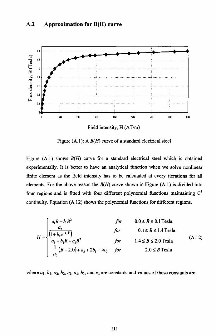
A.2 Approximation for B(H) curve
1.4
a:li 0.8.<;J~ 0.6"e~ 0.4
Ei:0.2
o __ ----~----~----~----~----~----~----~----~o lOO 200 300 400 500 600 700 800
Field intensity, H (AT/m)
Figure (A.l): A B(ll) curve ofa standard electrical steel
Figure (A. I ) shows B(ll) curve for a standard electrical steel which is obtained
experimentally. It is better to have an analytical function when we solve nonlinear
finite element as the field intensity has to be calculated at every iterations for all
elements. For the above reason the B(ll) curve shown in Figure (A.1) is divided into
four regions and is fitted with four different polynomial functions maintaining Cl
continuity. Equation (A.12) shows the polynomial functions for different regions.
a1B-b1B2 for 0.0 s B s 0.1 Tesla
a2 for 0.1 s B s 1.4 Tesla(I + b.e -C2B)H= (A.12)
a3 + b3B + c3B2 for 1.4 s B s 2.0TeslaI-(B - 2.0)+ a3 + 2b3 + 4c3 for 2.0 sBTeslaPo
where a .. b.. az, bi, C2, a3, bs, and C3 are constants and values of these constants are
III

al 69.80926049616697
b1 291.2027377442727
a2 -179.599730
b2 -59.6075740
C2 2.7802181
a3 1.261085222177513 x 10⁶
b3 -1.813387839003966 x lOb
C3 6.522906386158606e X 105
A.3 Approximating the stiffness matrix: what is important and
what is not
Equation (3.59) in Chapter 3 appears as
(A.13)
where [U] is the transformation matrix which determines the transformation of nodal
currents to the terminal currents. Generally [U] is a tall thin matrix.
Assert that [K] can be written in the following way
(A.14)
where
(A.IS)
i.e. [Hu] spans the same space as [U].
Also,
IV

(A.I6)
And further more
[Hy Y[U]= [Hy Y[Hu]= 0 (A.l7)
To find [Hu] the procedure is adopted. It is speculated that
[Hu]= [U][X] (A.I8)
[xl can be calculated as
(A.19)
(A.20)
The Cholesky decomposition can be used to evaluate the matrix [X]. The matrix [X]
can also be calculated by solving the eigenvalue problem. Once [Hu] is calculated
[Hy] is calculated as
(A.21)
Again assert that
(A.22)
The following procedure is adopted to calculate [Xu] and [x.].
(A.23)
v

Pre-multiplying by [n,Y and post-multiplying by [Hu] we can write Equation
(A.24) as
Similarly [Xv] can be calculated as
(A.27)
The main purpose of the calculation of [K]-1 is to evaluate inductance matrix, [L],
which is calculated using the formula
(A.28)
It is clear from Equation (A.28) that not all the entries of [K]-1 are relevant while
calculating the inductance matrix.
VI

A.4 Lagrange's equation of motion for coupled electrical and
mechanical dynamics
In this coupled system a mechanical process and an electromagnetic process are
coupled. The mechanical system is described by a generalised displacement vector,
{q} and electrical dynamics part of a R-L system is described by generalised
electrical quantity (charge), {Q}.
The Magnetic Field Energy, MFE can be written
MFE = _!_{QY [Lo(q,e)]{Q}2
(A.29)
Here {Q} is the electric current and [Lo(q,9)] is the inductance of the system which is
a function of displacement and rotational position of the rotor.
Similarly, the Kinetic Energy, KE of the system can be written as
KE = _!_ {qY [MHq}2
(A.30)
where [M] and {q} are the mass matrix and generalised velocity respectively.
Potential energy of the system, PE is
(A.31)
Here [K] and {q} are the stiffness matrix and generalised displacement vector
respectively. Dissipation function, F* is expressed as
(A.32)
VII

Here [R] is the resistance and [e] is the damping of the system. In the mechanical
dynamics {q} is the displacement vector and in electrical dynamics {Q} is the electric
charge vector. The Lagrangian of the electrical and mechanical coupled system is
L = KE{{q}, {q})+ MFE{{q}, {Q})- PE{{q}) (A.33)
Motion of the system is governed by the Lagrange equation
(A.34)
and
!!_ ( oL J - oL + of - Fdt d{q} d{q} d{q} - { 2}
(A.35)
where {F)} and {F2} are vectors the generalised forces. For the electrical system {F)}
is the vector generalised electric potentials and for the mechanical system {F2} is the
vector generalised mechanical forces.
Again from Equation (A.34) we get
(A.36)
(A.37)
(A.38)
From Equation (A.35) we get
VIn

Combining Equations (A.38) and (A.40)
IX
(A.39)
(A.40)
(A.41)

A.S Calculation of [Fo]based on the minimization of total resistive
losses
_[d ]{IsoY ~GoY [RE][Go]){Iso}=0dFo
d~o] {IsoY ([H~ I+ [H; HFo]T[RE][H~I+ [H; HFo])) {Iso}= 0
d~ol{I.or ([H;l+IFor[H~ r r [RE1[H;r + [HdIFol)){I.oH
_c!_{I y[[H~][RE1H~Y +[H;][REIH~HFo] I{I }=Od[Fo] BO +[Fof[H; Y[REIH; Y + [Fof[H; Y[REIH~][Fo]) so
2lH; j[REIH; J + 2[FoY[H; Y[REIH;] = 0
[Fo]=-[H; Y[RE1H; D1 QH;][RE1H~D
x
(A.42)
(A.43)
(A.44)
(A.45)
(A.46)
(A.47)

A.6 Effects of different number of modes of conductance in a
rotor bar
The machine considered is a 4-pole, 3-phase induction motor wound with double
layered windings. The stator of this machine has three independent currents. The
number of rotor bars is 32. This study provides the effects of different number of
modes of conductance in a rotor bar.
If two modes of conductance are considered for the rotor bar and the number of
harmonics for the Fourier approximation of the rotor bar is also five, the
transformations in Chapter 4 leads to a total of 20 independent rotor currents. The
stator and rotor currents can be written as
{
Rotor currentsStator currents (DC components),.---A----.. ....
{IRS2} = i1 ... i3 t.
Rotor currents Rotor currents Rotor currents Rotor currents } T(1st harmonics, cos) (1st harmonics, sin) (2nd harmonics, cos) (2nd harmonics, sin)~ ~ r-"----, ~
is . .. i6 i7 . .. i8 i9 . . . ilO ill . .. i12' .. i20
(A.48)
here i}, ... , ts are the three stator currents, i4 is the DC components of the rotor
currents, is, ... , i6 are the cosine components of the first harmonics of the rotor
currents and so on.
Similarly the stator and rotor currents for three, four and five modes of conductance
can be written as Equations (A.49), (A.50) and (A.51) respectively.
{
Rotor currentsStator currents (DC components)~ ,....--A--,
{IRS3} = i1 ••• i3 i4 is
Rotor currents Rotor currents Rotor currents Rotor currents } T(1st harmonics, cos) (1st harmonics, sin) (2nd harmonics, cos) (2nd harmonics, sin)
~ ~i6 . . . is i9 . .. ill i12 . . . i14 its ... i17' .. i29
(A.49)
XI

1Rotor currents Rotor currents Rotor currents Rotor currents Rotor currents } T
Stator currents (DC components) (Ist harmonics, cos) (Ist harmonics, sin) (2nd harmonics, cos) (2nd harmonics, sin)r--A----. ~ ~,..----A--....,..----A--.... ~
{IRs4} = i1 ••• i3 i, ... i6 i, ... ilO ill ... i14 i15 ... ilS i19 ... i22'" i3S
(A.SO)
{
Rotor currents Rotor currents Rotor currents Rotor currents Rotor currents } TStator currents (DC components) (1stharmonics, cos) (1stharmonics, sin) (2nd bannonics, cos) (2nd bannonics, sin)~ ~ ~ ~~,----J'---.
{IRs5} = i1 ... i3 i4 ... i7 is ... i12 i13 ... i17 ilS ... i23 i23 ... i27'" i47
(A.Sl)
Figure (A.2) shows the rotor currents for different modes of conductance corresponds
to the first modes of the cosine component of the 2nd harmonics and Figure (A.3)
shows the rotor currents for different modes of conductance corresponds to the first
modes of the sine component of the 2nd harmonics. It can be concluded that four
modes of conductance are enough to represent the currents in a rotor bar for this
machine.
XII

10~----,-----,-----,-----,-----,-----,-----,-----,
5~-----------;----
IIo
-5 --"------- -----,----------
-10~~2modes~~ 3modes~~4modes~~ 5modes
-15L_----~----~----~----~----~----~------~-----o 0_5 1_5 2 2.5 3 3.5 4
Time (sec)
Figure (A.2) shows the rotor currents for different modes of conductance corresponds
to the first modes of the cosine component of the 2nd harmonics
12
10
8
,..--._6<r:
<;»
til,_.4s::
Cl)..........:l 2u.....~...0 0.....0,_.0 -2~
-4
-6
-80 0.5
~~2modes-- 3modes-~~4modes
. ,- - - - - - -'_ - - - - - - - - - - - - ~ - - - - - - - - -- - - _j_-, , ,
, , ,-----------,----------- -,--------------,-------------,----- . ,----1-------------,------------
1.5 2Time (sec)
2.5 3 4
Figure (A.3) shows the rotor currents for different modes of conductance corresponds
to the first modes of the cosine component of the 2nd harmonics
XIII

APPENDIXB
B.1 Frequency response matrix
Consider a second-order system described by the three equations:
(B.I)
(B.2)
{y}= [SRY {q} (B.3)
If this system is classically-damped, then it is possible to define a coordinate
transformation in the form
(B.4)
with the effect that the equations of motion can be written as
(B.S)
(B.6)
(B.7)
with matrices [A], [r]and [I] all diagonal. It is obvious from Equations (B.!), (B.2),
(B.3) and (B.4) that
XN

[<I>LY =[TLY[SJ, [<I>RY =[TRY[SR] (B.8)
[AY = [TLY[KrnechITR], [rY = [TLY[DITR] and [IY = [TLY[MITR]
All of the matrices here are real-valued. The frequency-response matrix, [H{w)], is (no
x ni) where no represents the number of outputs (the dimension of {y}) and where n,
represents the number of inputs (the dimension of {u}). [H{w)] can be expressed in
terms of either the original representation of Equations (B.I), (B.2) and (B.3) or the
transformed (modal) representation of Equations (B.5), (B.6) and (B.7) thus
[H{w)] = [SRY[Krnech]+ jW[D]- w2 [M]f' [SL]= [<I>RJIA]+ jw[r]-w2[I]f'[<I>LY
(B.9)
A single entry of the frequency response matrix can be constructed as:
(B.10)
where 'L,jk represents the amount by which one unit of excitation at input degree of
freedom #j excites mode #k and 'R,ik represents the amount of output at output degree
of freedom #i is contributed by each mode #k.
xv

B.2 Supply Voltages and Stator Currents for No-Load conditions
from experimental rig
3.6 3.62 3.64 3.66 3.68 3.7
Time (sec)3.72 3.74 3.78
3.62 3.64 3.66 3.68 3.7 3.72 3.74 3.76 3.78
Time (sec)
Figure (B.2): Supply voltages and stator currents at no load condition for supply
frequency of 30 Hz
>''-.../
V 20OIl(':l....o>>-.0.. -200.::lo:
3.62 3.64 3.66 3.68 3.7 3.72 3.74 3.78
Time (sec)
6,---~---r---'----~--~--~--~~--'---~~ 4'-.../
~ 2t:V........::lU
3.62 3.64 3.66 3.68 3.7 3.72 3.74 3.76 3.78
Time (sec)
Figure (B.3): Supply voltages and stator currents at no load condition for supply
frequency of 35 Hz
XVI

3.6 3.62 3.64 3.66 3.68 3.7 3.72 3.74 3.76 3.78
Time (sec)
6'---~---'----r---~---o----~--~,,-.-- __:< 4'-'
~c::Q),_,_:::lU,_oro...VJ
3.62 3.64 3.66 3.68 3.7 3.72 3.74 3.76 3.78
Time (sec)
Figure (B.4): Supply voltages and stator currents at no load condition for supply
frequency of 40 Hz
3.62 3.64 3.66 3.68 3.7 3.72 3.74 3.76 3.78
Time (sec)
6c---~--~---.r---'-'-~----T<--~-'-'--~:< 4'-'
~cQ)
t::::lU,_oro...VJ
3.62 3.64 3.66 3.68 3.7 3.72 3.74 3.76 3.78
Time (sec)
Figure (B.S): Supply voltages and stator currents at no load condition for supply
frequency of 45 Hz
XVII

_50~ __ ~--~----L---~--~----~--_L--_J--~
3.6 3.62 3.64 3.66 3.68 3.7 3.72 3.74 3.76 3.78
Time (sec)
3.6 3.62 3.64 3.66 3.68 3.7 3.72 3.74 3.76 3.78
Time (sec)
Figure (B.6): Supply voltages and stator currents at no load condition for supply
frequency of 50 Hz
B.3 Equalizing Voltages and Currents for No-Load conditions
from experimental rig
,-.._ 5>'-'II)OJ)
~0>OJ)
_5L-~l- __ J_--_L--~--_J----~--~--J_--_L--~
3 3.1 3.2 3.3 3.4 3.5 3.6 37 3.8 3.9
Time (sec)
4
<: 1. 5 ,--- __ ~---.----,------r----r-----.----.----.-----.-----,'-'Vl
CII)......:JUOJ)
.:: -05Vl
~ -1 ----:J$ -1.5 L- __ l---J_--~--~--__L--__l----l.----..l---J____--_j
2 2.2 2.4 2.63.4 3.6 3.8 4
2.8 3 3.2
Time (sec)
Figure (B.7): Equalizing voltages and currents at no load condition for supply
frequency of 20 Hz
XVIII

~ 5>'-'II)01) 2.5E0>01)CN
til::lCTW.l
3.1 3.2 3.3 3.4 3.5 3.6 3.7 3.8 3.9 4
Time (sec)
til -1 - -- --- --r - - -- - - -- _- - - - -- - -- ---- _- -- - - - --,-- - ----,--- ----- -,- - - - - -- - -r-- - - - ---r -- ---
::l :: :
$ -1.5 '---_.L_____--'----_--'--_---'--_----'-_----'-' --'-----'-' -----'-'-----'
3 3.1 3.2 3.3 3.4 3.5 3.6 3.7 3.8 3.9
Time (sec)4
Figure CB.8): Equalizing voltages and currents at no load condition for supply
frequency of 25 Hz
> 5,--~-~-~-~-~--,r_-,_-,_-~-~'-'II)01)
Eo>01)c'N:.= -2.5 -til::l
$3.1 3.2 3.3 3.4 3.5 3.6 3.7 3.8 3.9 4
Time (sec)
~ 1.5 ,---r--~--,-----,------.----,--,___-_,__-,___-,'-'Vl.....CII).......::lU
, , I , , ,---.,---------,--------.,---------,-----·---,.--------r-------
I I I , , ,
I "' I
3.1 3.2 3.3 3.4 3.5 3.6 3.7 3.8 3.9 4
Time (sec)
Figure CB.9): Equalizing voltages and currents at no load condition for supply
frequency of 30 Hz
XIX

,-._ 5>'-'C)bl) 2.5~......0>bl)::::
3.1 3.2 3.3 3.4 3.5 3.6Time (sec)
3.7 3.8 3.9 4
~ 1.5~--~----~----~--~----~----~--~----~----~--~'-'rfJ......C~ 0.5;....;:lU 0bl)
c -0.5sr:
__ ~ L : ~ : ~ ~ _ _ _ _ _ .' _ _ _ _ _ _ _ _ __ ~ : _
~ -1;:l0"'~ -1.5L_--_L----~--~----~--~----~----~--~----~--~
3 3.1 3.2 3.3 3.4 3.5 3.6 3.7 3.8 3.9 4Time (sec)
, ,------, ----------,-----------,------- , ,----;-----------,--------
Figure (B.I 0): Equalizing voltages and currents at no load condition for supply
frequency of 35 Hz
> 5 ~--~--~--~--~~~----r_--,_--,_--_,--_,'-'(!)
~ 2.5.....o> °01):::
~ -2.5o:l::sCT~ _5L_--L---~ __ ~ __ _L~~ L_ __ ~ __ ~ __ ~ __ ~
3 3.1 3.2 3,3 3,4 3,5 3,6 3,7 3,8 3,9Time (sec)
4
~ 1,5<'-'<Jl....:::(!) 0,5,_,_::sU °01)
.::-0,5o:
o:l -1 - ---::s$ -1,5'---__ _j__ __ -'-- __ _j_ __ _L __ ___L __ -----' j___ __ i.-- __ -'-- __ __j
3 3,1
" "------.,---------,--------.,---------,---------r-
3,2 3,3 3,4 3,5 3,6 3,7 3,8 3,9Time (sec)
4
Figure (B. II ): Equalizing voltages and currents at no load condition for supply
frequency of 40 Hz
xx

,.-._ 5> I'-" I<l)OJ)
_g0>OJ)
3.1 3.2 3.3 3.4 3.5 3.6 3.7 3.8 3.9 4
Time (sec)
~ 1.5 r--,------,------,----,--------,--~--,_____-_._-__,__-~'-"VJ......::~ 0.5 1.....::::lU 0,OJ)
.:: -0.5 -IVJ
c<:l -1::l3 -1. 5 '--_.L_ _ _j__ _ _[___ _j__ _ __[__ ___J. __ L___-'---_--'--_~
3 3.1 3.2 3.3 3.4 3.5 3.6 3.7 3.8 3.9 4
Time (sec)
Figure (B.12): Equalizing voltages and currents at no load condition for supply
frequency of 45 Hz
~>'-'vbi)~.:::!o>bi)
.5N
o
3.1 3.2 3.3 3.4 3.5 3.6TIme (sec)
3.7 4
~ 1.5r--~--,----_____,_--__,__-~--___,__--,_____-~--,_-_,<;»
2 1I::v:...:...::lU
._-~ -1::l0"'~ -1. 5 '- _ _L__~ __ _L__~'_ _ _L__~ __ -'----_~ __ _L__~
3 3.1 3.2 3.3 3.4 3.5 3.6 3.7 3.8 3.9 4Time (sec)
Figure (B.13): Equalizing voltages and currents at no load condition for supply
frequency of 50 Hz
- - - - - - - - -~- - - - - - - - - - -'-, , - - - - - - - - - -: - - - - - - - - - - - ~ - - - - - - - - - + - - - - - - - - - - -: - - - - - - - - - - - ~ - - - - - - - - - - -: - -
XXI

C.I Comparison of results from MagFEA and MEGA
.. 10 ~ .. 10 ~.-2- .. 10 .... 10 ~.
20
....10I1
Airgap
-1+---- Central circle
Currentsheet
Iron
65
All dimensions are in mm
Figure (C.l): A simple electromagnetic device
A Bi : I I i I I
I . i I I I II I
i ! [I : I
It: iI
II
I, I
: I I! I II I
II
I I i I I
I I I' ! I
I I I
!I I
,I,
I I I '
=- -r- z. -t -r---r-----r- ~r-f-I
cD
Figure (C.2): FE mesh of the model
XXII

0151
i i
I I --Linear
0.1 ~ UUUUU muuUu. uuuu. m m u mm uumJ -- Non-linear I
I= 0.05i············j············· , , - : .
I-oo:tv~-~._········t· _.......................•••••~=
-0.1, ,
____________ J L J J , _
, " "
-0.15 , ,~- - - - - - - - - - - - - - - - - - - - - - - - - - -~- - - - - - - - - - - - - - - - - - - - - - - - --
0.03 0.04
Time (sec)Figure (C.3): x-component of the flux density for linear and non-linear case from
MagFEA in the middle of the airgap when Cl = 5 Azrnm'' and C2 = 0
0.01 0.02 0.05 0.06 0.07
0.1
0.08
0.06
0.04f='<;»
CO" 0.02;;.......c/l:::<!)
u><:=u..
-- Linear.................. -- Non-linear
____________ t- ., _
, ,, ,, ,
0.01 0.02 0.03 0.04
Time (sec)0.05 0.06 0.07
Figure (C.4): x-component of the flux density for linear and non-linear case from
MEGA in the middle of the airgap when Cl = 5 Azmm ' and C2 = 0
XXIII

o.5 ,--------~-_______:--____:_/:::;:________:-___;:::=c:=====:::c==~I ~
OAr Cl·II
••••••••••••••••••••••ol
--Linear I
-- Non-linear I. . I
....:..............•.............J
o
-0.1
-0.2L_--~--~--~--~--~--~--~o 0.01 0.02 0.03 0.04 0.05 0.06 0.07
Time (sec)Figure (C.S): y-component of the flux density for linear and non-linear case from
MagFEA in the middle of the airgap when Cl = 5 A'mm ' and C2 = 0
c5 r------:-----:--~:::::::::;_-__:_--~====~==~
OA ___ ~ L... _ _ _ _ _ _ _ _ _ _ _ _ _ _ _. .
--Linear
-0.1
. .-------------,--------------.--------------
t='<;»
co>'>......r./ls::<l) 0.1-0><:::su...
. .---- ---------,- ---- ---------r-
-0.2 L__ __l__ __ ___L __ ___L __ _I L._ __
o 0.01 0.02 0.03 0.04 0.05 0.06 0.07
Time (sec)
Figure (C.6): y-component of the flux density for linear and non-linear case from
MEGA in the middle of the airgap when Cl = S Azrnrrr' and C2 = 0
XXIV

0.3
0.2
0.1,--._,E--<;»COX
0:>.....u:s:::::Il)
-0.1'"0><:..2~
-0.2
-0.3
-0.40
--Linear
0.01 0.02 0.03 0.04 0.05 0.06 0.07Time (sec)
Figure (C.7): x-component of the flux density for linear and non-linear case from
MagFEA in the middle of the airgap when Cl = 10 Azrnm' and C2 = 0
0°1: I mmmm mummuuu\uuumm I;=~:~=:nearIj----- --- -- --~ ----- --- ---- --"----- ---------"--- ---- -------1
o
~ _. L L ...J _
, , ,
0.1
0.05
, ,_______________________ ...J _
, ,
-0_1 , ,- - - - - - - - - - - .... - - - -- - - - - - - - - .... - - - - - - - - - - - - - - .... - - - - - - - - - - - - - - ~- - - - - - - - - - - - --
----- .... --------------_ ... _------------_ ... --------------, , ,
-0_05
-0.15 ______________ .... L L _
, ,
-0.2 L-- __ ---'- L-- __ ---'- L-- __ _L_ __ ---' -"
o 0.01 0.02 0.03 0.04 0_05 0.06 0.07
Time (sec)
Figure (C.8): x-component of the flux density for linear and non-linear case from
MEGA in the middle of the airgap when Cl = 10 A/mm2 and C2 = 0
xxv

o
--Linear
0.8
0.6
0.4
0.2
-0.2
-0.4~--~--~--~--~--~--~--~o 0.01 0.02 0.03 0.04 0.05 0.06
Time (sec)0.07
Figure (C.9): y-component of the flux density for linear and non-linear case from
MagFEA in the middle of the airgap when Cl = 10 Azmm ' and C2 = 0
0.8
0.6~f--<'--'CO»;>......._(/J
::::::v 0.2"'Cl~:=r:i:
0
--Linear
0.01 0.02 0.03 0.04
Time (sec)0.05 0.06 0.07
Figure (C.lO): y-component of the flux density for linear and non-linear case from
MEGA in the middle of the airgap when Cl = 10 Azrnm' and C2 = 0
XXVI

0.4
0.3
0.2,-._,E-<<;» 0.1c:oX~.......- 0(/J
t::O..l'"0~ -0.1::s~
-0.2
-0.3
-0.40
--Linear-- Non-linear
0.03 0.04Time (sec)
Figure (C.ll): x-component of the flux density for linear and non-linear case from
MagFEA in the middle of the airgap when Cl = 15 A/mm 2 and C2 = 0
0.01 0.02 0.05 0.06 0.07
0.25~----~------~----~----~,-----~-----,------~
0.2
0.15:,:1
~ ;- _ - - - - - - - - -"1 __ ' l_ - - - - - - - - - - - - -;...- - - - - - - - - - - - - -,- - - - - - - - - - - - - - - "' - - -
--Linear---- Non-linear-- - - -- - .... - - - - - - - - - - - - - -- - - - - - - - - - - - - --,- - - - - - - -- - - - - - -~ -- - - - - - -- -- --
o
0.1 . .-------,----------------,--------------
:oX 0.05~......
-0.05 - - ------,--------------- .. --------------, ,, ,
-0.1 - - - - - - - - - - - - - -~ - - - - I -
, ,------------------,--------- ------,------
-0.15 _____________ ,_______, I
--------,----------------,--- , ,------,----------------,----------------,---------
O~2:c_-_- -_- -_- - -_- -_- -_l__-_- -_--_---_- -_--_J- -"c_- -_- _- -_- - -_- -_- ---'-'~L__- -_- -_- '. -_j- -"L__- -_- -_- -_- - _- - -_- -~- -_- - -_-_- -_- - _- - -_- -_l- ~_- - -_- -_- __ __j
o 0.01 0.02 0.03 0.04 0.05 0.06 0.07Time (sec)
Figure (C.12): x-component of the flux density for linear and non-linear case from
MEGA in the middle of the airgap when Cl = 15 Azrnm' and C2 = 0
XXVII

--f--.'-'~>.
;>-.~.- 0.5rFJ:::v"0~:J~
-- Linear-- Non-linear
o
-0.5~----~----~----~----~----~----~----~o 0.01 0.02 0.03 0.04 0.05 0.06 0.07Time (sec)
Figure (C.13): y-component of the flux density for linear and non-linear case from
MagFEA in the middle of the airgap when Cl = 15 Azmm' and C2 = 01.5 r-----:----:---:----~--i======c====::::;!
1 .----------
---- Linear-- Non-linear
0.5 --------------'----------------'-------------
o
0.01 0.02 0.03 0.04
Time (sec)0.05 0.06 0.07
Figure (C.14): y-component of the flux density for linear and non-linear case from
MEGA in the middle of the airgap when Cl = 15 Azrnm'' and C2 = 0
XXVIII
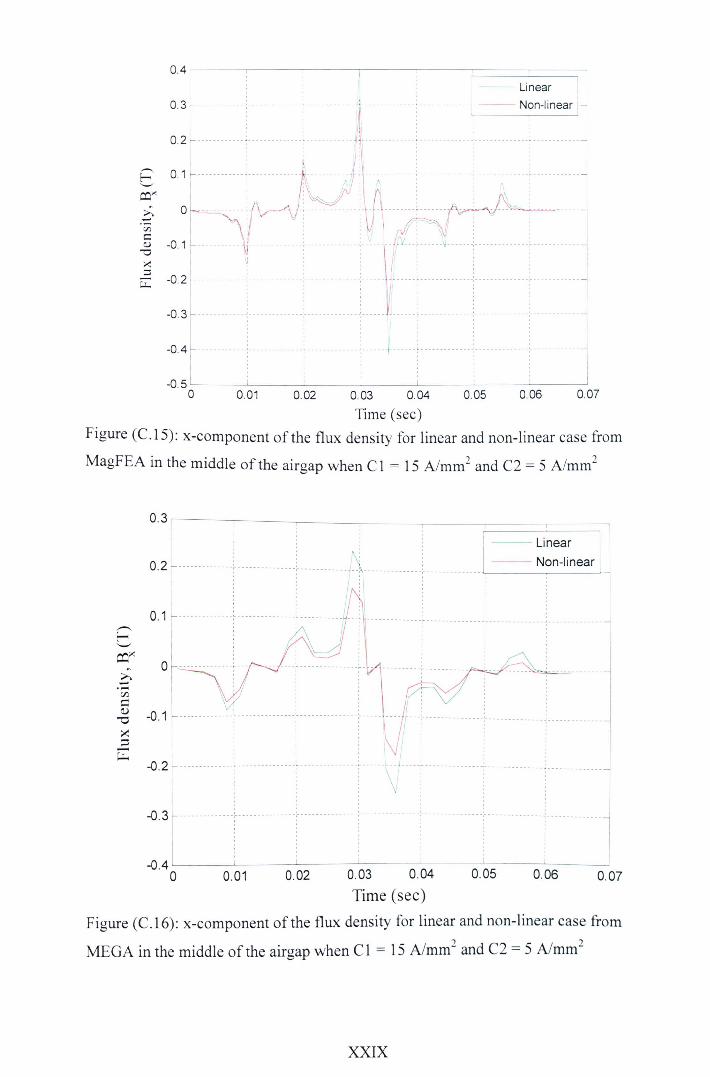
0.4
1
03,
02r-
E='I
0.1'-'
CO">. 0.....VJs::Il)
-0><::JCL.
i i
'I______________________________________ u _
!--Linear------------- -- Non-linearI
-0. 5 L__ __ _j__ __ __J__ __ ____j_ _l__ __ --'- __ -----'-__ ~
o 0.01 0.02 0.03 0.04 0.05 0.06 0.07
Time (sec)Figure (C.lS): x-component of the flux density for linear and non-linear case from
MagFEA in the middle of the airgap when Cl = 15 A/mm2 and C2 = 5 Azrnm''
-0.3 f- ---- ----- --- ;-- -- -- -- --- -- -~-- - - --- -- --- -~------, , ,
-0.4
0.3
0.2
0.1,--__t-<<;»COx
0:>......_C/Js:::0 -0.1~~~-~
-0.2
-0.3
-OA0
--Linear-- Non-linear
- ---,----- ----------,------------ --.,--------------
0.03 0.04
Time (sec)
Figure (C.16): x-component of the flux density for linear and non-linear case from
MEGA in the middle of the airgap when Cl = 15 Azrnm' and C2 = 5 Azmm'
0.01 0.02 0.05 0.06 0.07
XXIX

1.5
o ~["!!01··········· ...
-0.5
0.03 0.04
Time (sec)Figure (C.17): y-component of the flux density for linear and non-linear case from
MagFEA in the middle of the airgap when C2 = 15 A/mm2 and C2 = 5 Azmnr'
_1L_ ~ _J ~ _L L_ ~ ~
o 0.01 0.02 0.05 0.06 0.07
p<;»
co>' 0.5>.....VJCI!)
"0:><::Ju...
-- Linear
-- Non-linear
~ _ ~ .J ,__
, ,
------------""--------------,-----, ,
0.03 0.04
Time (sec)
Figure (C.l8): y-component of the flux density for linear and non-linear case from
MEGA in the middle of the airgap when C2 = 15 Azmnr' and C2 = 5 Azmm'
xxx
Copyright © 2022 FDOKUMEN