arX

iv:h

ep-p

h/01

0332

0v2

14

May

200

1

SUSX-TH/01-016

EDM Constraints in Supersymmetric Theories

S. Abel1,2, S. Khalil1,3, and O. Lebedev1

1Centre for Theoretical Physics, University of Sussex, Brighton BN1 9QJ, U. K.

2IPPP, University of Durham, South Rd., Durham DH1 3LE , U. K.

3Ain Shams University, Faculty of Science, Cairo, 11566, Egypt.

Abstract

We systematically analyze constraints on supersymmetric theories imposed bythe experimental bounds on the electron, neutron, and mercury electric dipolemoments. We critically reappraise the known mechanisms to suppress theEDMs and conclude that only the scenarios with approximate CP-symmetryor flavour-off-diagonal CP violation remain attractive after the addition of themercury EDM constraint.

1 Introduction

There are a number of reasons to suspect that there are additional sources of CP viola-tion beyond those of the Standard Model (given by θ and δKM). The most compellingone is that the SM is unable to explain the cosmological baryon asymmetry of our uni-verse. Also, the Standard Model is very unlikely to be the “ultimate” theory of nature.Most extensions of the SM bring in new sources of CP-violation. In particular, themost attractive one – the Minimal Supersymmetric Standard Model (MSSM) allowsfor new sources of CP violation in both supersymmetry-breaking and supersymmetry-conserving sectors, and there are no compelling arguments for them to be zero. Inaddition, the improving precision in the measurements of the CP-observables such asACP (B → ψKs) [1] may soon reveal deviations from the SM predictions.

The most stringent constraints on models with additional sources of CP violationcome from continued efforts to measure the electric dipole moments (EDM) of theneutron [2], electron [3], and mercury atom [4]

dn < 6.3 × 10−26 e cm (90%CL),

de < 4.3 × 10−27 e cm ,

dHg < 2.1 × 10−28 e cm . (1)

1

With the expected improvements in experimental precision, the EDM is likely to beone of the most important tests for physics beyond the Standard Model for some timeto come, and EDMs will remain a difficult hurdle for supersymmetric theories if theyare to allow sufficient baryogenesis. Indeed it is remarkable that the SM contribution tothe EDM of the neutron is of order 10−30 e cm, whereas the “generic” supersymmetricvalue is 10−22e cm.

In this paper we analyze neutron, electron, and mercury EDMs in the context ofR-parity conserving supersymmetric theories. In particular, we reconsider the knownmechanisms to suppress EDMs in light of the recently reported bound on the mercuryEDM [4]. These include SUSY models with small CP phases, models with heavysfermions, the cancellation scenario, and models with flavour off-diagonal CP violation.We also study to what extent different scenarios rely on assumptions about the neutronstructure, i.e. chiral quark model vs parton model.

The paper is organized as follows. In section 2 we present general formulae for theEDMs and discuss their model-dependence. In section 3 we define our supersymmetricframework and present all relevant supersymmetric contributions to the EDMs. Inparticular, we analyze the importance of the two-loop Barr-Zee and Weinberg typeEDM contributions. Section 4 is devoted to the study of the EDM suppression mecha-nisms. First we consider in detail the “canonical” scenarios: suppression due to smallCP phases or heavy sfermions. Second, in the context of the cancellation scenario, weanalyze the possibility of the EDM cancellations in two classes of models: mSUGRA-like models with nontrivial gaugino phases and D-brane models. Finally, we discussthe EDM suppression in models with flavour-off-diagonal CP violation. In addition,we present new model-independent bounds on the sfermion mass insertions imposed bythe electron, neutron, and mercury electric dipole moments. In section 5 we overviewand discuss our results.

2 Electron, neutron, and mercury electric dipole

moments

Let us first summarize the contributions to the three most significant EDMs, beginningwith the most reliable, the electron EDM.

2.1 Electron EDM

The electron EDM is defined by the effective CP-violating interaction

L = − i

2deeσµνγ5e F

µν , (2)

where F µν is the electromagnetic field strength. The experimental bound on the elec-tron EDM is derived from the electric dipole moment of the thallium atom and is givenby [3]

de < 4 × 10−27e cm . (3)

2

In supersymmetric models, the electron EDM arises due to CP-violating 1-loop dia-grams with the chargino and neutralino exchange:

de = dχ+

e + dχ0

e . (4)

Since the EEDM calculation involves little uncertainty it allows to extract reliablebounds on the CP-violating SUSY phases.

2.2 Neutron EDM

The neutron EDM has contributions from a number of CP-violating operators involv-ing quarks, gluons, and photons. The most important ones include the electric andchromoelectric dipole operators, and the Weinberg three-gluon operator:

L = − i

2dE

q qσµνγ5q Fµν − i

2dC

q qσµνγ5Taq Gaµν

− 1

6dGfabcGaµρG

ρbνGcλσǫ

µνλσ , (5)

where Gaµν is the gluon field strength, T a and fabc are the SU(3) generators and groupstructure coefficients, respectively. Given these operators, it is however a nontrivial taskto evaluate the neutron EDM since assumptions about the neutron internal structureare necessary. In what follows we will study two models, namely the quark chiral modeland the quark parton model. Neither of these models is sufficiently reliable by itself [5],however a power of the combined analysis should provide an insight into implications ofthe bound on the neutron EDM and in particular comparing them gives some indicationof the importance of these systematic errors in, for example, cancellations. A betterjustified approach to the neutron EDM based on the QCD sum rules has appeared in[8] and earlier work [9], [13]. We note that in any case the NEDM calculations involveuncertain hadronic parameters such as the quark masses and thus these calculationshave a status of estimates. The major conclusions of the present work are independentof the specifics of the neutron model.

i. Chiral quark model. This is a nonrelativistic model which relates the neutronEDM to the EDMs of the valence quarks with the help of the SU(6) coefficients:

dn =4

3dd −

1

3du . (6)

The quark EDMs can be estimated via Naive Dimensional Analysis [6] as

dq = ηEdEq + ηC e

4πdC

q + ηG eΛ

4πdG , (7)

where the QCD correction factors are given by ηE = 1.53, ηC ≃ ηG ≃ 3.4, andΛ ≃ 1.19 GeV is the chiral symmetry breaking scale. We use the numerical values forthese coefficients as given in [7]. The parameters ηC,G involve considerable uncertainties

3

steming from the fact that the strong coupling constant at low energies is unknown.Another weak side of the model is that it neglects the sea quark contributions whichplay an important role in the nucleon spin structure.

The supersymmetric contributions to the dipole moments of the individual quarksresult from the 1-loop gluino, chargino, neutralino exchange diagrams

dE,Cq = dg (E,C)

q + dχ+ (E,C)q + dχ0 (E,C)

q , (8)

and from the 2-loop gluino-quark-squark diagrams which generate dG.

ii. Parton quark model. This model is based on the isospin symmetry andknown contributions of different quarks to the spin of the proton [10]. The quantities∆q defined as 〈n|1

2qγµγ5q|n〉 = ∆q Sµ, where Sµ is the neutron spin, are related by

the isospin symmetry to the quantities (∆q)p which are measured in the deep inelasticscattering (and other) experiments, i.e. ∆u = (∆d)p, ∆d = (∆u)p, and ∆s = (∆s)p. Tobe exact, the neutron EDM depends on the (yet unknown) tensor charges rather thanthese axial charges. The main assumption of the model is that the quark contributionsto the NEDM are weighted by the same factors ∆i, i.e. [10]

dn = ηE(∆ddEd + ∆ud

Eu + ∆sd

Es ) . (9)

In our numerical analysis we use the following values for these quantities ∆d = 0.746,∆u = −0.508, and ∆s = −0.226 as they appear in the analysis of Ref.[11]. As before,we have

dEq = dg (E)

q + dχ+ (E)q + dχ0 (E)

q . (10)

The major difference from the chiral quark model is a large strange quark contribution(which is likely to be an overestimate [5]). In particular, due to the large strangeand charm quark masses, the strange quark contribution dominates in most regionsof the parameter space. This leads to considerable numerical differences between thepredictions of the two models.

The current experimental limit on the neutron EDM is [2]

dn < 6.3 × 10−26e cm . (11)

2.3 Mercury EDM

The EDM of the mercury atom results mostly from T-odd nuclear forces in the mercurynucleus [12], which induce the effective interaction of the type (I · ∇)δ(r) between theelectron and the nucleus of spin I [5]. In turn, the T-odd nuclear forces arise due to theeffective 4-fermion interaction ppniγ5n. It has been argued [5] that the mercury EDMis primarily sensitive to the chromoelectric dipole moments of the quarks and the limit[4]

dHg < 2.1 × 10−28e cm (12)

can be translated into

|dCd − dC

u − 0.012dCs |/gs < 7 × 10−27cm , (13)

4

where gs is the strong coupling constant. As in the parton neutron model, thereis a considerable strange quark contribution. The relative coefficients of the quarkcontributions in (13) are known better than those for the neutron, however the overallnormalization is still not free of uncertainties [13].

3 The EDMs in SUSY models

We will study supersymmetric models with the following high energy scale soft breakingpotential

VSB = m20αφ

∗αφα − (BµH1H2 + h.c.) + (AlY

lij H1lLie

∗Rj + AdY

dij H1qLid

∗Rj

− AuYuij H2qLiu

∗Rj + h.c.) +

1

2(m3gg +m2W aW a +m1BB) , (14)

where φα denotes all the scalars of the theory. We generally allow for Al 6= Au 6= Ad

as well as nonuniversal gaugino and scalar masses, which is important for the analysisof D-brane models. The µ, B, Aα, and mi parameters can be complex, however twoof their phases can be eliminated by the U(1)R and U(1)PQ transformations underwhich these parameters behave as spurions. The Peccei-Quinn transformation actson the Higgs doublets and the “right-handed” superfields in such a way that all theinteractions but those which mix the two doublets are invariant. The Peccei-Quinncharges are QPQ(µ) = QPQ(Bµ), QPQ(A) = QPQ(mi) = 0. The U(1)R transformsthe Grassmann variable θ → θeiα and the fields in such a way that the integral of thesuperpotential over the Grassmann variables is invariant, i.e. the U(1)R charge of thesuperpotential is 2. As a result, QR(Bµ) = QR(µ) − 2, QR(A) = QR(mi) = −2. Thesix physical CP-phases of the theory are invariant under both U(1)R and U(1)PQ, andcan be chosen as

Arg(A∗dmi) , Arg((Bµ)∗µAα) , (15)

where i = 1, 2, 3 and α = d, u, l. All other CP-phases can be expressed as theirlinear combinations. If the A-terms are universal, there are four physical phasesArg(A∗mi) , Arg((Bµ)∗µA).

It is customary to choose the phase convention in which the Higgs potential param-eter Bµ is real. In this case, the physical phases become Arg(A∗

dmi) and Arg(µAα). Ifuniversality is assumed, the number of physical phases reduces to two. In what followswe will set m2 to be real by a U(1)R rotation.

Nonuniversality will play a crucial role in the D-brane and flavour models’ analysis,but otherwise does not lead to different conclusions for the models we study. Thus wewill assume universal A-terms and gaugino masses unless otherwise specified.

In what follows we use tan β, m0, A, mi as input parameters and obtain low energyquantities via the MSSM renormalization group equations (RGE). We also assumeradiative electroweak symmetry breaking, i.e. that the magnitude of the µ parameteris given (at tree level) by

|µ|2 =m2

H1−m2

H2tan2 β

tan2 β − 1− 1

2m2

Z . (16)

5

The phase of µ is an input parameter and is RG-invariant. Our numerical results aresensitive to the quark masses which we fix at theMZ scale to be: mui

= (0.005, 1.40, 165)GeV and mdi

= (0.010, 0.194, 3.54) GeV. The light quark masses are poorly determined(in fact mu = 0 is not excluded) which results in the uncertainties of the EDM nor-malization; for definiteness, we have chosen the light quark masses as they appear in[7]. The GUT scale is assumed to be 2 × 1016 GeV.

It is well known that O(1) supersymmetric CP phases generally lead to unaccept-ably large electric dipole moments which constitutes the SUSY CP problem. In thispaper we consider different mechanisms for suppressing EDMs and analyze them indetail.

3.1 Leading SUSY contributions to the EDMs

In this subsection we list formulae for individual supersymmetric contributions to theEDMs due to the Feynman diagrams in Fig.1. In our presentation we follow the workof Ibrahim and Nath [7].

∼g , ∼χ0∼χ+ ,

∼ g

γ

f

f fL R

∼g ∼ qq

Figure 1: Leading SUSY contributions to the EDMs. The photon and gluon lines areto be attached to the loop in all possible ways.

Neglecting the flavour mixing, the electromagnetic contributions to the fermionEDMs are given by [7]:

dg (E)q /e =

−2αs

3π

2∑

k=1

Im(Γ1kq )

mg

M2qk

Qq B( m2

g

M2qk

)

,

dχ+ (E)u /e =

−αem

4π sin2 θW

2∑

k=1

2∑

i=1

Im(Γuik)mχ+

i

M2dk

[

Qd B(m2

χ+

i

M2dk

)

+ (Qu −Qd) A(m2

χ+

i

M2dk

)]

,

dχ+ (E)d /e =

−αem

4π sin2 θW

2∑

k=1

2∑

i=1

Im(Γdik)mχ+

i

M2uk

[

Qu B(m2

χ+

i

M2uk

)

+ (Qd −Qu) A(m2

χ+

i

M2uk

)]

,

dχ+

e /e =αem

4π sin2 θW

2∑

i=1

mχ+

i

m2ν

Im(Γei) A(m2

χ+

i

m2ν

)

,

6

dχ0 (E)f /e =

αem

4π sin2 θW

2∑

k=1

4∑

i=1

Im(ηfik)mχ0

i

M2fk

Qf B(m2

χ0i

M2fk

)

. (17)

HereΓ1k

q = e−iφ3Dq2kD∗q1k , (18)

with φ3 being the gluino phase and Dq defined by D†qM

2qDq = diag(M2

q1,M2

q2). The

sfermion mass matrix M2f

is given by

M2f

=(

ML2 +mf

2 +M2z (1

2−Qf sin2 θW ) cos 2β mf(A

∗f − µRf )

mf (Af − µ∗Rf ) M2R +mf

2 +M2zQf sin2 θW cos 2β

)

,

where Rf = cot β (tanβ) for I3 = 1/2 (−1/2). The chargino vertex Γfik is defined as

Γuik = κuV∗i2Dd1k(U

∗i1D

∗d1k − κdU

∗i2D

∗d2k) ,

Γdik = κdU∗i2Du1k(V

∗i1D

∗u1k − κuV

∗i2D

∗u2k) (19)

and analogously for the electron; here U and V are the unitary matrices diagonalizingthe chargino mass matrix: U∗Mχ+V −1 = diag(mχ+

1, mχ+

2). The quantities κf are the

Yukawa couplings

κu =mu√

2mW sin β, κd,e =

md,e√2mW cosβ

. (20)

The neutralino vertex ηfik is given by

ηfik =[

−√

2{tan θW (Qf − I3f)X1i + I3f

X2i}D∗f1k − κfXbiD

∗f2k

]

×[√

2 tan θWQfX1iDf2k − κfXbiDf1k

]

, (21)

where I3 is the third component of the isospin, b = 3 (4) for I3 = −1/2 (1/2),and X is the unitary matrix diagonalizing the neutralino mass matrix: XTMχ0X =diag(mχ0

1, mχ0

2, mχ0

3, mχ0

4). In our convention the mass matrix eigenvalues are positive

and ordered as mχ01> mχ0

2> ... (this holds for all mass matrices in the paper). The

loop functions A(r), B(r), and C(r) are defined by

A(r) =1

2(1 − r)2

(

3 − r +2 ln r

1 − r

)

,

B(r) =1

2(r − 1)2

(

1 + r +2r ln r

1 − r

)

,

C(r) =1

6(r − 1)2

(

10r − 26 +2r ln r

1 − r− 18 ln r

1 − r

)

. (22)

The chromoelectric contributions to the quark EDMs are given by

dg (C)q =

gsαs

4π

2∑

k=1

Im(Γ1kq )

mg

M2qk

C( m2

g

M2qk

)

,

dχ+ (C)q =

−g2gs

16π2

2∑

k=1

2∑

i=1

Im(Γqik)mχ+

i

M2qk

B(m2

χ+

i

M2qk

)

,

dχ0 (C)q =

gsg2

16π2

2∑

k=1

4∑

i=1

Im(ηqik)mχ0

i

M2qk

B(m2

χ0i

M2qk

)

. (23)

7

Finally, the contribution to the Weinberg operator [14] from the two-loop gluino-top-stop and gluino-bottom-sbottom diagrams reads

dG = −3αsmt

(

gs

4π

)3

Im(Γ12t )

z1 − z2m3

g

H(z1, z2, zt) + (t→ b) , (24)

where zi =(

Mti

mg

)2

, zt =(

mt

mg

)2

. The two-loop function H(z1, z2, zt) is given by [15]

H(z1, z2, zt) =1

2

∫ 1

0dx∫ 1

0du∫ 1

0dy x(1 − x)u

N1N2

D4, (25)

where

N1 = u(1 − x) + ztx(1 − x)(1 − u) − 2ux[z1y + z2(1 − y)] ,

N2 = (1 − x)2(1 − u)2 + u2 − 1

9x2(1 − u)2 ,

D = u(1 − x) + ztx(1 − x)(1 − u) + ux[z1y + z2(1 − y)] . (26)

The numerical behaviour of this function was studied in [15]. We emphasize that theb-quark contribution is significant and often exceeds the top one.

Before we proceed to the discussion of the EDM suppression mechanisms, let usconsider the effect of other potentially nonnegligible two-loop contributions.

3.2 Barr-Zee type EDM contributions

In view of considerable recent interest in the subject we will consider the two-loopBarr-Zee type contributions separately. We will follow the work of Chang, Keung, andPilaftsis [16].

gγ,

∼q

gγ,

f f fL R R

a gγ,

gγ,∼

a

q

f f fL R R

Figure 2: Barr-Zee type contributions to the EDMs.

In Ref.[17] Barr and Zee have presented two-loop Higgs-mediated EDM contribu-tions which can be competetive with the Weinberg three-gluon operator. A supersym-metric version of the Barr-Zee graphs (Fig.2) was studied in [16]. In what follows we

8

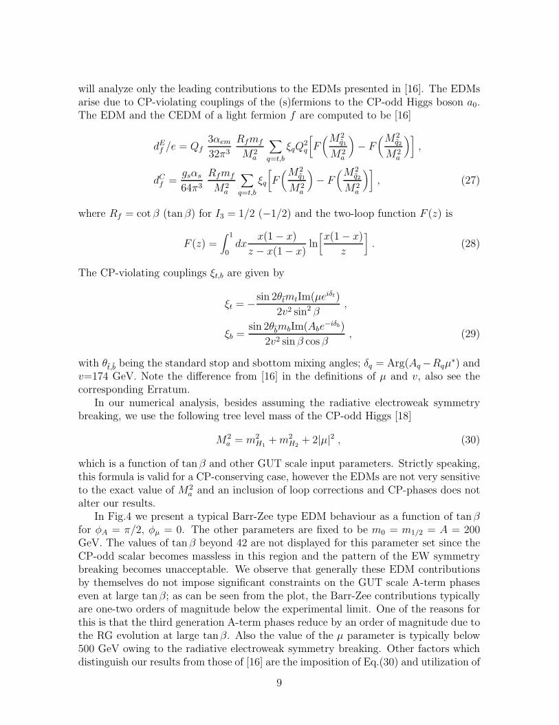
will analyze only the leading contributions to the EDMs presented in [16]. The EDMsarise due to CP-violating couplings of the (s)fermions to the CP-odd Higgs boson a0.The EDM and the CEDM of a light fermion f are computed to be [16]

dEf /e = Qf

3αem

32π3

Rfmf

M2a

∑

q=t,b

ξqQ2q

[

F(M2

q1

M2a

)

− F(M2

q2

M2a

)]

,

dCf =

gsαs

64π3

Rfmf

M2a

∑

q=t,b

ξq

[

F(M2

q1

M2a

)

− F(M2

q2

M2a

)]

, (27)

where Rf = cot β (tanβ) for I3 = 1/2 (−1/2) and the two-loop function F (z) is

F (z) =∫ 1

0dx

x(1 − x)

z − x(1 − x)ln[

x(1 − x)

z

]

. (28)

The CP-violating couplings ξt,b are given by

ξt = −sin 2θtmtIm(µeiδt)

2v2 sin2 β,

ξb =sin 2θbmbIm(Abe

−iδb)

2v2 sin β cos β, (29)

with θt,b being the standard stop and sbottom mixing angles; δq = Arg(Aq −Rqµ∗) and

v=174 GeV. Note the difference from [16] in the definitions of µ and v, also see thecorresponding Erratum.

In our numerical analysis, besides assuming the radiative electroweak symmetrybreaking, we use the following tree level mass of the CP-odd Higgs [18]

M2a = m2

H1+m2

H2+ 2|µ|2 , (30)

which is a function of tan β and other GUT scale input parameters. Strictly speaking,this formula is valid for a CP-conserving case, however the EDMs are not very sensitiveto the exact value of M2

a and an inclusion of loop corrections and CP-phases does notalter our results.

In Fig.4 we present a typical Barr-Zee type EDM behaviour as a function of tanβfor φA = π/2, φµ = 0. The other parameters are fixed to be m0 = m1/2 = A = 200GeV. The values of tan β beyond 42 are not displayed for this parameter set since theCP-odd scalar becomes massless in this region and the pattern of the EW symmetrybreaking becomes unacceptable. We observe that generally these EDM contributionsby themselves do not impose significant constraints on the GUT scale A-term phaseseven at large tanβ; as can be seen from the plot, the Barr-Zee contributions typicallyare one-two orders of magnitude below the experimental limit. One of the reasons forthis is that the third generation A-term phases reduce by an order of magnitude due tothe RG evolution at large tanβ. Also the value of the µ parameter is typically below500 GeV owing to the radiative electroweak symmetry breaking. Other factors whichdistinguish our results from those of [16] are the imposition of Eq.(30) and utilization of

9

the chiral quark neutron model1. For comparison, in Fig.4 we provide the contributionof the Weinberg operator which also arises at the two-loop level.

The constraints become more restrictive for larger A-terms (∼ 3m0) and largerm0/m3 ratios. In Fig.5 we set m0 = 500 GeV, m1/2 = 200 GeV, and A = 600 GeV. Inthis case the A-term phase is not “diluted” as much as before and for some parametersthe Barr-Zee EDMs can be close to the experimental limit. A similar effect can beachieved in models with non-universal gaugino masses by introducing a O(1) gluinophase. With the parameter set of Fig.5 the CP-odd Higgs becomes unacceptably lightaround tanβ ≃ 36.

¿From the point of view of low energy theory, the Barr-Zee type contributionscan provide useful constraints on the phases of the third generation A-terms [16],[19].One can imagine a situation in which the first two generation CP-violating effects aresuppressed (as in the decoupling scenario), then the EDMs would constrain the thirdgeneration phases. We find however that typically the Weinberg three-gluon operatoris considerably more sensitive to such phases and provides more severe constraints evenat large tan β2. For example, for the parameters of Figs.4 and 5 the contribution ofthe Weinberg operator exceeds that of the Barr-Zee type graphs by one-two orders ofmagnitude.

Finally, the Z- and W-mediated Barr-Zee type graphs have been analyzed in [20]and found to be significantly smaller than those considered above. A number of othersubleading two loop contributions such as the gluino CEDM-induced quark EDMs, etc.have been studied in [21].

Although taken into account, this entire class of diagrams is numerically unimpor-tant in our analysis.

4 Suppression of the EDMs in SUSY models

4.1 Small CP-phases

For a light (below 1 TeV) supersymmetric spectrum, the SUSY CP phases have tobe small in order to satisfy the experimental EDM bounds (unless EDM cancellationsoccur). In Figs.6-8 we illustrate the EDMs behaviour as a function of the CP-phasesin the mSUGRA-type models, where we have set m0 = m1/2 = A = 200 GeV. At lowtan β, the EDM constraints impose the following bounds (at the GUT scale):

φA ≤ 10−2 − 10−1 ,

φµ ≤ 10−3 − 10−2 ,

φgaug. ≤ 10−2 . (31)

For tan β > 3, these bounds become even stricter (for φµ and φgaug. the bounds areroughly inversely proportional to tanβ). We note that φA is less constrained than φµ

1 We observe similar behaviour in the parton quark model.2The Weinberg operator contribution can be suppressed by increasing the gluino mass. However, in

mSUGRA the Barr-Zee type contributions will also get a suppression factor due to the RG “dilution”of the phases of the third generation A-terms.

10

and φgaug.. There are two reasons for that: first, φA is reduced by the RG running fromthe GUT scale down to the electroweak scale and, second, the phase of the (δd

11)LR

mass insertion which gives the dominant contribution to the EDMs is more sensitiveto φµ and φgaug. due to |A| < µ tanβ.

SUSY models with small CP-phases can be motivated by the approximate CPsymmetry [22]. The well established experimental results exhibit small degree of CPviolation. Thus it is conceivable that all existing CP-phases are small, including theCKM phase. The smallness of CP violation can be explained, for example, by a smallratio of the scale at which the CP symmetry gets broken spontaneously and the scaleat which it is communicated to the observable sector.

Currently the CKM phase is consistent with zero and it could be supersymmetrythat is responsible for the observed values of ε and ε′. This does not require largesupersymmetric phases. In fact in models with non-universal A-terms ε and ε′ caneven be saturated with O(10−2) phase of the mass insertion (δd

12)LR [23]. In this case,|(δd

12)LR| is required to be O(10−3) which naturally appears in models with matrix-factorizable A-terms of the form B · Yα · C, where B and C are flavour matrices. TheEDM bounds serve to constrain the flavour structure of B and C. Another possibilityto produce the desired (δd

12)LR is to use asymmetric A-term textures in string-motivatedmodels (where the standard supergravity relation Aij = AijYij is assumed).

Encouragingly, the phase of the µ-term of order 10−2 may be sufficient to producethe observed baryon asymmetry [24], which is in marginal agreement with the EDMbounds. The hypothesis of the approximate CP symmetry is currently being tested inthe B physics experiments where the Standard Model predicts large CP-asymmetries.It is noteworthy that the smallness of the CP-phases in this picture does not constitutefine-tuning according to the t’Hooft’s criterion [25] since setting them to zero wouldincrease the symmetry of the theory.

We remark that small CP-phases may also arise due to the dynamics of the system.For instance, in weakly coupled heterotic string models, small soft and CKM phasesarise when the T-moduli get VEV’s close to the edge of the fundamental domainwhich is often the case [26]. This mechanism however relies on the assumption thatthe dilaton has a real VEV, so this model as it stands does not solve the SUSY CPproblem. Nevertheless, it may serve as a step toward a consistent string model withnaturally small CP phases.

Note that EDMs constrain only the physical phases (15). One can imagine asituation when the individual phases are O(1) whereas the physical ones are small. Thisoccurs for example in gauge mediated SUSY breaking models, see [22] and referencestherein.

4.2 Heavy SUSY scalars

This possibility is based on the decoupling of heavy supersymmetric particles. Even ifone allows O(1) CP violating phases, their effect will be negligible if the SUSY spectrumis sufficiently heavy [27]. Generally, SUSY fermions are required to be lighter than theSUSY scalars by, for example, cosmological considerations. So the decoupling scenario

11

can be implemented with heavy sfermions only. Here the SUSY contributions to theEDMs are suppressed even with maximal SUSY phases because the squarks in the loopare very heavy and the mixing angles are small.

In Fig.9 we display the EDMs as functions of the universal scalar mass parameterm0

for the mSUGRA model with maximal CP-phases φµ = φA = π/2 and m1/2 = A = 200GeV. We observe that all EDM constraints except for that of the electron require m0

to be around 5 TeV or more. The mercury constraint is the strongest one and requires

(m0)decoupl. ≃ 10 TeV . (32)

This leads to a serious fine-tuning problem. Recall that one of the primary motivationsfor supersymmetry was a solution to the naturalness problem. Certainly this motivationwill be entirely lost if a SUSY model reintroduces the same problem in a different sector,i.e. for example a large hierarchy between the scalar mass and the electroweak scale.

The degree of fine-tuning can be quantified as follows. The Z boson mass is deter-mined at tree level by

1

2m2

Z =m2

H1−m2

H2tan2 β

tan2 β − 1− µ2 . (33)

One can define the sensitivity coefficients [28],[29]

ci ≡∣

∣

∣

∣

∂ lnm2Z

∂ ln a2i

∣

∣

∣

∣

, (34)

where ai are the high energy scale input parameters such as m1/2, m0, etc. Note thatµ is treated here as an independent input parameter. A value of ci much greater thanone would indicate a large degree of fine-tuning. The Higgs mass parameters are quitesensitive to m0, so for m0=10 TeV we find

cm0∼ 5000 (35)

for the parameters of Fig.9. For the universal scalar mass of 5 (3) TeV the sensitivitycoefficient reduces to 1300 (500). This clearly indicates an unacceptable degree offine-tuning.

This problem can be mitigated in models with focus point supersymmetry, i.e. whenmH2

is insensitive to m0 [29]. However, this mechanism works for m0 no greater than2-3 TeV which is not sufficient to suppress the EDMs. Another interesting possibility ispresented by models with a radiatively driven inverted mass hierarchy, i.e. the modelsin which a large hierarchy between the Higgs and the first two generations scalar massesis created radiatively [30]. However, a successful implementation of this idea is far fromtrivial [31]. One can also break the scalar mass universality at the high energy scale[32]. In this case, either a mass hierarchy appears already in the soft breaking termsor certain relations among the soft parameters must be imposed (for a review see [33]).These significant complications disfavour the decoupling scenario as a way to solve theSUSY CP problem, yet it remains a possibility.

Note that the decoupling scenario rules out supersymmetry as a possible explana-tion of the recently observed 2.6 σ deviation in the muon g−2 from the SM prediction

12

[34]. This scenario may also lead to cosmological difficulties, in particular with therelic abundance of the LSPs since the LSP annihilation cross section falls rapidly asmsfermion increases. Concerning the other phenomenological consequences, we remarkthat the SUSY contributions to the CP-observables involving the first two generations(such as ε, ε′) are negligible, although those involving the third generation may beconsiderable. The corresponding CP-phases are constrained through the Weinberg op-erator contribution to the neutron EDM, which typically prohibits the maximal phaseφAt,b

∣

∣

∣

GUT= π/2 while still allowing for smaller O(1) phases (Fig.4).

4.3 EDM cancellations

The cancellation scenario is based on the fact that large cancellations among differ-ent contributions to the EDMs are possible in certain regions of the parameter space[7],[36],[37],[11] which allow for O(1) flavour− independent CP phases. Although notparticularly well motivated, this possibility is interesting since, when supplementedwith a real non-trivial flavour structure, it allows for significant supersymmetric con-tributions to CP observables including those in the B system. In this case, the SMpredictions can be significantly altered leading for instance to a nonclosure of the uni-tarity triangle (see M. Brhlik et al. in [23]). Given the appropriate A-terms’ flavourstructures, the parameters ε and ε′ can be of completely supersymmetric nature [23].Large flavour-independent SUSY phases may also be responsible for electroweak baryo-genesis [35]. Thus the cancellation scenario presents a interesting alternative to thedecoupling and approximate CP solutions.

For the case of the electron, the EDM cancellations occur between the charginoand the neutralino contributions. For the case of the neutron and mercury, there arecancellations between the gluino and the chargino contributions as well as cancellationsamong contributions of different quarks to the total EDM. A number of approximateformulae quantifying the cancellations are presented in Refs.[7],[36].

In what follows we examine the cancellation scenario in the universal and nonuni-versal cases, with the latter being motivated by Type I string models. We note thatthe CP phases are to be understood modulo π.

4.3.1 EDM cancellations in mSUGRA-type models.

These are mSUGRA-type models allowing different phases for different gaugino masseswhile keeping their magnitudes the same. As we will see, mSUGRA models with zerogaugino phases can realize the cancellation scenario. An introduction of the gauginophases makes the cancellations much harder to achieve (if possible at all) and leads toa much higher degree of fine-tuning. The parameters allowing the EDM cancellationsstrongly depend on the neutron model. For example, in the parton model, it is moredifficult to achieve these cancellations due to the large strange quark contribution.Therefore, one cannot restrict the parameter space in a model-independent way andcaution is needed when dealing with the parameters allowed by the cancellations.

In mSUGRA, the EDM cancellations can occur simultaneously for the electron,

13

neutron, and mercury along a band in the (φA, φµ) plane (Figs.10 and 11). However, inthis case the mercury constraint requires the µ phase to be O(10−2) and the magnitudeof the A-terms to be suppressed (∼ 0.1m0) which results in only a small effect of theA-terms on the phase of the corresponding mass insertion. This is to be contrastedwith simultaneous EEDM/NEDM cancellations which allow for φµ ∼ O(10−1) andA ∼ m0 [11],[36]. In that case the individual contributions to the EDMs exceeded theexperimental limit by an order of magnitude (or more). Owing to the addition of themercury constraint, the EDM cancellations become much milder as illustrated in Fig.12.For example, without these cancellations the EDMs would exceed the experimentallimit only by a factor of a few. Obviously, the border between the cancellation and thesmall phases scenarios becomes blurred. This is even more so at larger tan β (Fig.13),in which case the cancellation band becomes narrower and the limits on φµ becometighter. We note that there could exist some points which allow for φµ ∼ O(10−1) [38],however these are rare exceptions and such points do not form a band.

As noted in Ref.[11], in the case of zero gaugino phases, the band in the (φA, φµ)plane where the cancellations occur can approximately be described by a relation

φµ ≃ −a sinφA , (36)

where a is a constant depending on the parameters of the model which representsthe maximal allowed phase φµ. For example, for the chiral quark neutron model andtan β = 3, m0 = m1/2 = 200 GeV, and |A| = 40 GeV (parameters of Fig.10), a = 0.017.Of course, the value of a depends on the input parameters such as the quark masses,the GUT scale, the SUSY scale, etc. and also involves numerical uncertainties, socaution is needed when treating this number. The maximal allowed φµ is roughlyinversely proportional to tanβ, e.g. for tan β = 10 we have a = 0.005 (Fig.13). Inthe case of the parton model, the cancellations occur, for example, with a = 0.006 andtan β = 3, m0 = m1/2 = 200 GeV, and |A| = 20 GeV (Fig.11). As mentioned earlier,the cancellations are harder to achieve in the parton model, which results in tighterlimits on φµ (∼ O(10−3)). In both cases φµ is restricted to be of order 10−3 − 10−2,whereas φA can be arbitrary (however physical effects due to φA will be suppressedbecause of the small magnitude of A). The GUT parameters given above imply thatthe squark masses at low energies are about 500 GeV, so these bounds can be relaxedonly if the squark masses are over 1 TeV.

If the gluino phase is turned on, simultaneous EEDM, NEDM, and mercury EDMcancellations are not possible. The gluino phase affects the NEDM cancellation bandby altering the relation (36):

φµ ≃ −a sin(φA + α) − c , (37)

while leaving the EEDM cancellation band almost intact (Fig.14). An introductionof the bino phase φ1 qualitatively has the same “off-setting” effect on the EEDMcancellation band as the gluino phase does on that of the NEDM (Fig.15). Note thatthe bino phase has no significant effect on the neutron and mercury cancellation bandssince the neutralino contribution in both cases is small. When both the gluino and

14

bino phases are present (and fixed), simultaneous electron, neutron, and mercury EDMscancellations do not appear to be possible along a band. The reason is that the mercuryEDM depends on φ3 more strongly than the NEDM does, so that an introduction ofthe gluino phase splits the bands where the mercury and neutron EDM cancellationsoccur as illustrated in Figs.14 and 15. Thus we see that zero gaugino phases are muchmore preferred by the cancellation scenario.

The cancellation scenario involves a significant fine-tuning. Indeed, restricting thephases to the band where the cancellations occur does not increase the symmetry of themodel and thus is unnatural according to the t’Hooft’s criterion [25]. It is a non-trivialtask to quantify the degree of fine-tuning in this case. One possibility is to define anEDM sensitivity coefficient with respect to the CP-phases, in analogy with Eq.34. Wetypically find it to be between 30 and 100 on the cancellation band. This howeverrepresents only a local behaviour of the EDMs. In other words it shows how easy it isto spoil the cancellations without a reference to how improbable it is to achieve suchcancellations in the first place. An alternative way to quantify the degree of fine-tuningis simply to estimate the probability that a random small area in the (φµ, φA) plane willsafisfy the cancellation condition. Since any point is not prefered over any other pointby the underlying theory, this should give a fairly good idea of the minimal degree offine-tuning needed. From Fig.10 we obtain

fine − tuning ∼ (probability)−1 >∼ 102 . (38)

Note that this estimate does not take into account the fine-tuning of the other softbreaking parameters which is necessary to allow for simultaneous EEDM, NEDM, andmercury EDM cancellations. Other estimates give a similar number for the universalcase, whereas for the nonuniversal case the degree of fine-tuning drastically increases:only one out of 105 random points in the parameter space satisfies the cancellationcondition [38].

4.3.2 EDM cancellations in D-brane models.

Let us first briefly review basic ideas of D-brane models (see also Refs.[39] and [40]).Recent studies of type I strings have shown that it is possible to construct a numberof models with non–universal soft SUSY breaking terms which are phenomenologicallyinteresting. Type I models can contain 9-branes, 5i-branes, 7i-branes, and 3-braneswhere the index i = 1, 2, 3 denotes the complex compact coordinate which is includedin the 5-brane world volume or which is orthogonal to the 7-brane world volume.However, to preserve N = 1 supersymmetry in D = 4 not all of these branes can bepresent simultaneously and we can have (at most) either D9-branes with D5i-branesor D3-branes with D7i-branes.

Gauge symmetry groups are associated with stacks of branes located “on top ofeach other”. A stack of N branes corresponds to the group U(N). The matter fieldsare associated with open strings which start and end on the branes. These stringsmay be attached to either the same stack of branes or two different sets of braneswhich have overlapping world volumes. The ends of the string carry quantum numbers

15

associated with the symmetry groups of the branes. For example, the quark fields haveto be attached to the U(3) set of branes, while the quark doublet fields also have to beattached to the U(2) set of branes. Given a brane configuration, the Standard Modelfields are constructed according to their quantum numbers.

The SM gauge group can be obtained in the context of D-brane scenarios fromU(3) × U(2) × U(1), where the U(3) arises from three coincident branes, U(2) arisesfrom two coincident D-branes and U(1) from one D-brane. As explained in detail inRef.[40], there are different possibilities for embedding the SM gauge groups withinthese D-branes. It was shown that if the SM gauge groups come from the same setof D-branes, one cannot produce the correct values for the gauge couplings αj(MZ)and the presence of additional matter (doublets and triplets) is necessary to obtainthe experimental values of the couplings [41]. On the other hand, the assumption thatthe SM gauge groups originate from different sets of D-branes leads in a natural wayto intermediate values for the string scale MS ≃ 1010−12 GeV [40]. In this case, theanalysis of the soft terms has been done under the assumption that only the dilatonand moduli fields contribute to supersymmetry breaking and it has been found thatthese soft terms are generically non–universal. The MSSM fields arising from openstrings are shown in Fig.3. For example, the up quark singlets uc are states of the typeC953 , the quark doublets are C951 , etc. The presence of extra (Dq) branes which arenot associated with the SM gauge groups is often necessary to reproduce the correcthypercharge and to cancel non-vanishing tadpoles.

wb

g

ce

Q

L,

U(1)U(3) U(2) Lc

u

cd

eH1

H2

uc

D53D51

D52

D9

Figure 3: Embedding the SM gauge group within different sets of D-branes. The extraDq brane (52) is marked by a cross.

Recently there has been a considerable interest in supersymmetric models derivedfrom D-branes [42],[43]. In a toy model of Ref.[42], the gauge group SU(3)c × U(1)Y

16

was associated with 51 branes and SU(2)L was associated with 52 branes. It wasshown that in this model the gaugino masses are non–universal (M1 = M3 6= M2) sothat the physical CP phases are φ1 = φ3, φA and φµ. Non-universality of the gauginomasses allowed to enlarge the regions of the parameter space where the NEDM/EEDMcancellations occured. However, such a model is oversimplified and the relation φ1 =φ3 6= φ2 does not appear to hold in more realistic models [44]. In what follows we willconsider the EDM cancellations in this and a more realistic D-brane models.

The model in which U(3), U(2), and U(1) originate from different sets of branesis phenomenologically interesting. In this case one naturally obtains an intermediatestring scale (1010 − 1012 GeV), although higher values up to 1016 GeV are still al-lowed. Both the up and the down type Yukawa interactions are allowed, while thatfor the leptons typically vanishes (depending on further details of the model) [40].The (anomaly-free) hypercharge is expressed in terms of the U(1) charges Q1,2,3 of theU(1)1,2,3 groups:

Y = −1

3Q3 −

1

2Q2 +Q1 , (39)

with the following (Q3, Q2, Q1) charge assignment:

q = (1,−1, 0) , uc = (−1, 0,−1) , dc = (−1, 0, 0) , (40)

l = (0, 1, 0) , ec = (0, 0, 1) ,

H2 = (0, 1, 1) , H1 = (0, 1, 0) .

The gaugino masses in this model are given by

M3 =√

3m3/2 sin θ e−iαs , (41)

M2 =√

3m3/2 Θ1 cos θ e−iα1 ,

MY =√

3m3/2 αY (MS)

×(

2

α1(MS)Θ3 cos θe−iα3 +

1

α2(MS)Θ1 cos θe−iα1 +

2

3α3(MS)sin θe−iαs

)

,

where1

αY (MS)=

2

α1(MS)+

1

α2(MS)+

2

3α3(MS). (42)

Here αk correspond to the gauge couplings of the U(k) branes. As shown in Ref.[40],α1(MS) ≃ 0.1 leads to the string scale MS ≈ 1012 GeV. The parameters θ and Θi

parameterize supersymmetry breaking in the usual way [39]:

F S =√

3(S + S∗)m3/2 sin θ e−iαs ,

F i =√

3(Ti + T ∗i )m3/2 cos θ Θie

−iαi , (43)

and i = 1, 2, 3 labels the three complex compact dimensions.The soft scalar masses are given by

m2q = m2

3/2

[

1 − 3

2

(

1 − Θ21

)

cos2 θ]

,

17

m2dc = m2

3/2

[

1 − 3

2

(

1 − Θ22

)

cos2 θ]

,

m2uc = m2

3/2

[

1 − 3

2

(

1 − Θ23

)

cos2 θ]

,

m2ec = m2

3/2

[

1 − 3

2

(

sin2 θ + Θ21 cos2 θ

)

]

,

m2l = m2

3/2

[

1 − 3

2

(

sin2 θ + Θ23 cos2 θ

)

]

,

m2H2

= m23/2

[

1 − 3

2

(

sin2 θ + Θ22 cos2 θ

)

]

,

m2H1

= m2l , (44)

and the trilinear parameters are

Au =

√3

2m3/2

[(

Θ2e−iα2 − Θ1e

−iα1 − Θ3e−iα3

)

cos θ − sin θ e−iαs

]

, (45)

Ad =

√3

2m3/2

[(

Θ3e−iα3 − Θ1e

−iα1 − Θ2e−iα2

)

cos θ − sin θ e−iαs

]

, (46)

Ae = 0 . (47)

We observe that the angles Θi and θ are quite constrained if we are to avoid negativemass-squared’s for squarks and sleptons. In what follows we set Θ3 = 0 and α1 = α2;then the soft terms are parameterized in terms of the phase φ ≡ α1 − αs.

In Fig.16 we display the bands allowed by the electron (red), neutron (green),and mercury (blue) EDMs. In this figure, we set m3/2 = 150 GeV, tan β = 3,Θ2

1 = Θ22 = 1/2, cos2 θ = 2 sin2 θ = 2/3, and α1(MS) ∼ 1 with MS being the GUT

scale. For the plot to be more illustrative, we do not impose any additional constraintsbesides the EDM ones (i.e. bounds on the chargino and slepton masses, etc.). It isclear that even though simultaneous EEDM/NEDM cancellations allow the phase φto be O(1), an addition of the mercury constraint requires all phases to be very small(modulo π) and thus practically rules out the cancellation scenario in this context.The situation becomes even worse in the case of an intermediate string scale ∼ 1012

GeV (i.e. α1(MS) ∼ 0.1), see Fig.17. We find it quite generic that the mercury EDMbehaviour in D-brane models is very different from that of the electron and neutronand thus is crucial in constraining the parameter space. The major difference fromthe mSUGRA-type models with fixed φY and φ3 is that the phase of the A-terms iscorrelated with the gaugino phases resulting in the cancellation bands which are notdescribed by a simple relation φµ ≃ −a sin(φA + α) − c.

Next we consider the model of Ref.[42]. The (corrected) soft terms for this modelread (for Θ3 = 0)

MY = M3 = −A =√

3m3/2 cos θ Θ1e−iα1 ,

M2 =√

3m3/2 cos θ Θ2e−iα2 ,

m2L = m2

3/2(1 − 3

2sin2 θ);

m2R = m2

3/2(1 − 3 cos2 θ Θ22) . (48)

18

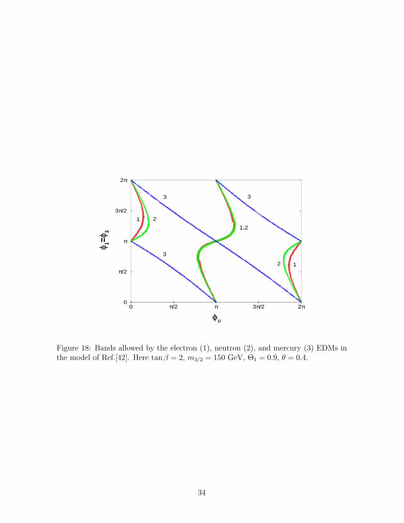
To illustrate the EDM constraints, we choose the parameters which allow for simulta-neous EEDM/NEDM cancellations, namely m3/2 = 150 GeV, tanβ = 2, Θ1 = 0.9, andθ = 0.4 as given in Ref.[42]. Fig.18 shows that the mercury constraint has the samebehaviour as in the model considered above and rules out large CP-phases.

We see that the cancellation scenario in simple models faces a number of difficulties.Presently available string-motivated models with non-universal gaugino masses cannotaccommodate simultaneous electron, neutron, and mercury EDM cancellations. In themSUGRA, such cancellations are possible but require a significant fine-tuning. Theaddition of the mercury EDM bound restricts the phase of the µ term to be O(10−2) ifwe are to achieve the EDM cancellations along a band in the (φA, φµ) plane. Withoutan additional SUSY flavour structure, the CP-phases allowed by the cancellations willhave very small observable effects. Even in a more general situation (unconstrainedMSSM), the phases allowed by the EDM cancellations typically lead to small CP-asymmetries ( <∼ 1%) in collider experiments [38]. Testing the cancellation scenarioexperimentally may prove to be a challenge.

4.4 Flavour-off-diagonal CP violation

This is one of the more attractive possibilities to avoid overproduction of EDMs inSUSY models. Nonobservation of EDMs may imply that CP-violation has a flavour-off-diagonal character just like in the Standard Model. The origin of CP-violationin this case is closely related to the origin of the flavour structures rather than theorigin of supersymmetry breaking. While models with flavour-off-diagonal CP violationnaturally avoid the EDM problem, they have testable effects in K and B physics.

This class of models requires hermitian Yukawa matrices and A-terms, which forcesthe flavour-diagonal phases to vanish (up to small RG corrections) in any basis. Theflavour-independent quantities such as the µ-term, gaugino masses, etc. are real. This isnaturally implemented in left-right symmetric models [45] and models with a horizontalflavour symmetry [47].

In the left-right models, the hermiticity of the Yukawas and A-terms as well as thereality of the µ-term is forced by the left-right symmetry. The SU(2)L gaugino massis in general complex, so in order to suppress the EDMs the additional assumptionof its reality is needed. The phenomenology of such models in the context of up-down unification has been studied in [46]. The left-right symmetry appears to be toorestrictive in this case to satisfy all of the phenomenological constraints; however thedecisive test will be undertaken at the B factories.

Another possibility is based on a horizontal U(3)H symmetry [47]. HermitianYukawa matrices may appear due to a (gauged) horizontal symmetry U(3)H which getsbroken spontaneously by the VEVs of the real adjoint fields T a

α (a = 1..9; α = u, d, l, ..)[48]. Some of these real VEV’s also break CP since some of the components of T a

α areCP-odd. As a result, CP violation appears in the superpotential through complexYukawa couplings, whereas the µ-term is real since it arises from a U(3)H invariantcombination of the type T a

αTaβ . An effective U(3)H-invariant superpotential of the type

W = gH

MH1Qi(T

ad λ

a)ijDj produces the Yukawa matrix (Y d)ij = gH

M〈T a

d 〉(λa)ij , where

19

λ0 is proportional to the unit matrix and λ1−8 are the Gell-Mann matrices. Note thatthe real fields T a

α may only come from a non-supersymmetric (anti-brane) sector. IfT a

α are the scalar components of chiral multiplets, they are intrinsically complex andhermitian Yukawas in this case arise only if the VEVs of T a

α are real.The gaugino masses in this model are not forced to be real by symmetry. One has

to make an additional assumption that either the gaugino masses are universal andthe corresponding phase can be rotated away or that the SUSY breaking dynamicsconserve CP which seems natural if CP breaking is associated with the origin of flavourstructures. In other words, the SUSY breaking auxiliary fields get real VEVs as a resultof the underlying dynamics such as the dilaton stabilization in Type I string models[49] or the effective potential minimization in heterotic string models [50]. Further,if the Kahler potential is either generation independent or left-right symmetric, theA-terms are hermitian [47]. This leads to very small phases in the flavour-diagonalmass insertions which are responsible for generating EDMs and the EDM bounds areeasily satisfied.

Both the left-right model and the model with a horizontal symmetry mitigate thestrong CP-problem (under the additional assumptions given above). The θ parametervanishes at both the tree and the leading log one-loop levels. However neither of thesemodels solves the problem completely due to the significant one loop finite correctionswhich appear mostly due to a non-degeneracy of the squark masses and a misalignmentbetween the Yukawas and the A-terms [51].

In this class of models we have the following setting at the high energy scale:

Yα = Y †α , Aα = A†

α ,

Arg(Mk) = Arg(µ) = 0 . (49)

Generally, the off-diagonal elements of the A-terms can have O(1) phases withoutviolating the EDM constraints. Due to the RG effects, large phases in the soft trilinearcouplings involving the third generation generate small phases in the flavour-diagonalmass insertions for the light generations, and thus induce the EDMs. For example, theA-terms of the form3

Ad = Au = m0

1 a12 a13

a∗12 1 a23

a∗13 a∗23 a33

(50)

and the following GUT-scale hermitian Yukawa matrices

Y u =

4.1 × 10−4 6.9 × 10−4 i −1.4 × 10−2

−6.9 × 10−4 i 3.5 × 10−3 −1.4 × 10−5 i−1.4 × 10−2 1.4 × 10−5 i 6.9 × 10−1

,

Y d =

1.3 × 10−4 2.0 × 10−4 + 1.8 × 10−4 i −4.4 × 10−4

2.0 × 10−4 − 1.8 × 10−4 i 9.3 × 10−4 7.0 × 10−4 i−4.4 × 10−4 −7.0 × 10−4 i 1.9 × 10−2

.

3The standard supergravity relation (Aα)ij = (Aα)ij(Yα)ij for the trilinear soft couplings is as-sumed.

20

typically induce the mercury EDM of the order of the experimental limit if a33 is oforder 1, whereas the induced NEDM is 1-2 orders of magnitude below the experimentallimit. If one uses Yukawa textures with smaller Y α

13, this RG effect will be suppressedrendering the induced mercury EDM far below the experimental limit.

The supersymmetric contribution to the ε′ parameter is suppressed in models withhermitian flavour structures4 [47]. This occurs due to severe cancellations betweenthe contributions involving (δd

12)LR and (δd12)RL mass insertions (we use the standard

definitions of [53]). Due to the hermiticity (δd12)LR ≃ (δd

12)RL, whereas they contribute

to ε′ with opposite signs. Typically we find∣

∣

∣Im[

(δd12)LR − (δd

12)RL

]∣

∣

∣ < 10−6 which

produces ε′ an order of magnitude below the experimental limit [53]. On the otherhand, similar cancellations do not occur for the ε parameter and the SUSY contributionto ε can be even dominant. The value of (δd

12)LR which saturates the observed |ε| ≃2.26× 10−3 is given by

√

|Im(δd12)

2LR| ≃ 3.5× 10−4 for the gluino and squark masses of

500 GeV [53].For completeness, we provide the bounds on the imaginary parts of the mass inser-

tions

(δd(u)ii )LR =

1

m2((A

d(u)†SCKM)iiv1(2) − Y

d(u)i µv2(1)) (51)

derived from the leading gluino contributions to the electromagnetic (NEDM) operatorand the bino contribution to the electron EDM. We update the bounds of Ref.[53] andalso include the QCD correction factor. The advantage of the mass insertion approachis that it allows to obtain model independent bounds and thus is quite useful whendealing with complicated flavour structures. For comparison we present the bounds forthe chiral (Table 1) and the parton (Table 2) neutron models.

A drastic improvement of the bounds comes from the addition of the mercuryEDM constraint. Using the expressions for the chromomagnetic moments of Ref.[37],in Table 3 we present the bounds on the mass insertions from the gluino contributions tothe mercury EDM. For |Im(δd

11)LR)| and |Im(δu11)LR)| these bounds turn out to be very

strict, more than an order of magnitude stricter than those imposed by the NEDM. Thisseverely restricts the CP-asymmetry ACP (b → sγ) in models with hermitian flavourstructures. The reason is that in order to obtain a large (∼ 10%) SUSY contributionto this observable, the elements of the A-terms involving the third generation have tobe larger than 1. This induces via the RG running a considerable |Im(δd,u

11 )LR)|, oftenin conflict with the bounds of Table 3. We find that with the above Yukawa texturesACP (b → sγ) is allowed to be no more than 2-3%. One can relax this constraint byusing different hermitian textures, especially with suppressed Y α

13. In this case theCP-asymmetry can be as large as 6-7%.

To conclude this section, we remark that the problem of baryogenesis in this classof models requires careful investigation and at the moment it is unclear whether or notlarge flavour off-diagonal SUSY phases can produce sufficient baryon asymmetry of theuniverse.

4For phenomenology of models with non-universal (but non-hermitian) A-terms see also [52].

21

5 Discussion and conclusions

We have systematically analyzed constraints on supersymmetric models imposed by theexperimental bounds on the electron, neutron, and mercury electric dipole moments.We find that the EDMs can be suppressed in SUSY models with

1) small SUSY CP-phases ( <∼ 10−2). This possibility can be motivated by theapproximate CP-symmetry which also implies that the CKM phase is small. Thisprovides testable signatures for B-factories’ experiments.

2) heavy SUSY scalars, msfermion ∼ 10 TeV. In this class of models there is a largehierarchy between the SUSY and electroweak scales, which is hard to realize withoutan extreme fine-tuning.

3) EDM cancellations. We have analyzed the possibility of such cancellations inD-brane and mSUGRA-like models with nontrivial gaugino phases. We find that, withthe addition of the mercury EDM constraint, only the EDM cancellations in mSUGRA(φ1 ≃ φ3 ≃ 0) survive in any considerable part of the parameter space. Even in this casethe cancellations require small φµ ∼ 10−2 and suppressed |A| (∼ 0.1m0). As a result,the border between the small phases and the cancellation scenarios fades away. Inaddition to the finetuning problem, models with the EDM cancellations lack predictivepower as it is unclear whether the allowed CP-phases can have observable effects.

4) flavour-off-diagonal CP violation. This can occur in models with CP-conservingSUSY breaking dynamics and hermitian flavour structures. Such models allow for O(1)flavour off-diagonal phases which can have significant effects in K and B physics.

It is also possible to combine different mechanisms to suppress the EDMs. Forexample, a “hybrid” of the decoupling and the cancellation scenarios was consideredin Ref.[54]. Such models seem to share shortcomings of both “parents” without anapparent advantage over either of them.

There is also a rather radical proposal that all gaugino masses and the A-terms arevanishingly small [55]. Clearly this eliminates all of the physical phases in Eq.(15) andthus produces no CP violation. Such a strong assumption requires a firm motivationsuch as the continuous R-symmetry. However, by the same token, the R-symmetryeliminates the Bµ term thereby leading to a very light CP-odd Higgs boson. Such ascenario faces a number of difficulties with experimental results.

To summarize, we have studied the supersymmetric CP problem taking into ac-count all of the current EDM constraints. Our conclusion is that there remain twoattractive ways to avoid overproduction of the EDMs in SUSY models. The first pos-sibility is that CP is an approximate symmetry of nature and the second one is thatCP violation has a flavour off-diagonal character just as in the Standard Model.

Acknowledgements. S.A. and O.L. were supported by the PPARC Opportunitygrant, S.K. was supported by the PPARC SPG. The authors are grateful to D. Bailin,M. Brhlik, T. Ibrahim, C. Munoz, and M. Pospelov for useful discussions, and to M.Gomez and D. Cerdeno for their help in the computing aspects of this work.

22

References

[1] T. Affolder et al., CDF collaboration, Phys. Rev. D61 (2000), 072005; B. Aubert et

al., BaBar collaboration, hep-ex/0102030 ; A. Abashian et al., Belle collaboration,hep-ex/0102018.

[2] P.G. Harris et al., Phys. Rev. Lett. 82 (1999), 904; see also the discussion in S.K.Lamoreaux and R. Golub, Phys. Rev. D61 (2000), 051301.

[3] E.D. Commins et al., Phys. Rev. A50 (1994), 2960.

[4] M.V. Romalis, W.C. Griffith, and E.N. Fortson, Phys. Rev. Lett. 86, 2505 (2001);J.P. Jacobs et al., Phys. Rev. Lett. 71 (1993), 3782.

[5] T. Falk, K.A. Olive, M. Pospelov, R. Roiban, Nucl. Phys. B560 (1999), 3.

[6] H. Georgi and A. Manohar, Nucl. Phys. B234, 189 (1984); R. Arnowitt, J.L.Lopez and D.V. Nanopoulos, Phys. Rev. D42 (1990), 2423; R. Arnowitt, M.J.Duff and K.S. Stelle, Phys. Rev. D43 (1991), 3085.

[7] T. Ibrahim and P. Nath, Phys. Rev. D57 (1998), 478; Errata-ibid. D58, 019901(1998); ibid. D60, 019901 (1999); Phys. Lett. B418, 98 (1998); Phys. Rev. D58,111301 (1998); Erratum-ibid. D60, 099902 (1999).

[8] M. Pospelov and A. Ritz, Phys. Rev. D 63, 073015 (2001).

[9] V.M. Khatsimovsky, I.B. Khriplovich and A.R. Zhitnitsky, Z. Phys. C36 (1987),455; V.M. Khatsimovsky, I.B. Khriplovich and A.S. Yelkhovsky, Annals Phys. 186

(1988), 1; V.M. Khatsimovsky and I.B. Khriplovich, Phys. Lett. B296 (1992), 219.

[10] J. Ellis, R. Flores, Phys. Lett. B377 (1996), 83.

[11] A. Bartl, T. Gajdosik, W. Porod, P. Stockinger, and H. Stremnitzer, Phys. Rev.D60 (1999), 073003.

[12] W. Fischler, S. Paban and S. Thomas, Phys. Lett. B 289, 373 (1992).

[13] I.B. Khriplovich and S.K. Lamoreaux, “CP Violation Without Strangeness”,Springer, 1997.

[14] S. Weinberg, Phys. Rev. Lett. 63, 2333 (1989); E. Braaten, C. Li and T. Yuan,Phys. Rev. Lett. 64, 1709 (1990).

[15] J. Dai, H. Dykstra, R. G. Leigh, S. Paban and D. Dicus, Phys. Lett. B237, 216(1990).

[16] D. Chang, W. Keung and A. Pilaftsis, Phys. Rev. Lett. 82, 900 (1999); Erratum-ibid. 83, 3972 (1999).

[17] S. M. Barr and A. Zee, Phys. Rev. Lett. 65, 21 (1990).

23

[18] J. F. Gunion and H. E. Haber, Nucl. Phys. B272, 1 (1986).

[19] S. Baek and P. Ko, Phys. Rev. Lett. 83, 488 (1999).

[20] D. Chang, W. Chang and W. Keung, Phys. Lett. B478, 239 (2000); A. Pilaftsis,Phys. Lett. B471, 174 (1999).

[21] A. Pilaftsis, Phys. Rev. D 62, 016007 (2000).

[22] M. Dine, E. Kramer, Y. Nir, Y. Shadmi, hep-ph/0101092; G. Eyal and Y. Nir,Nucl. Phys. B528 (1998), 21; and references therein.

[23] A. Masiero and H. Murayama, Phys. Rev. Lett. 83 (1999), 907; S. Khalil andT. Kobayashi, Phys. Lett. B 460, 341 (1999); M. Brhlik, L. Everett, G. L. Kane,S. F. King and O. Lebedev, Phys. Rev. Lett. 84 (2000), 3041.

[24] M. Carena, M. Quiros, A. Riotto, I. Vilja and C. E. Wagner, Nucl. Phys. B 503,387 (1997).

[25] G. ’t Hooft, in Recent Advances in Gauge Theories, Proceedings of the CargeseSummer Institute, Cargese, France, 1979, edited by G. t’ Hooft et al., NATOAdvanced Study Institute Series B; Physics Vol.59 (Plenum, New York, 1980).

[26] D. Bailin, G. V. Kraniotis and A. Love, Nucl. Phys. B 518, 92 (1998); J. Giedt,Nucl. Phys. B 595, 3 (2001); T. Dent, hep-th/0011294.

[27] P. Nath, Phys. Rev. Lett. 66 (1991), 2565; Y. Kizukuri and N. Oshimo, Phys.Rev. D46 (1992) 3025.

[28] R. Barbieri and G.F. Giudice, Nucl. Phys. B306 (1988), 63; J. Ellis, K. Enqvist,D.V. Nanopoulos, F. Zwirner, Mod. Phys. Lett. A1 (1986), 57; G.G. Ross andR.G. Roberts, Nucl. Phys. B377 (1992), 571.

[29] J.L. Feng, K.T. Matchev, and T. Moroi, Phys. Rev. D61 (2000), 075005; Phys.Rev. Lett. 84 (2000), 2322.

[30] J. L. Feng, C. Kolda and N. Polonsky, Nucl. Phys. B 546, 3 (1999).

[31] H. Baer, C. Balazs, M. Brhlik, P. Mercadante, X. Tata, Y. Wang, hep-ph/0102156.

[32] S. Dimopoulos and G. F. Giudice, Phys. Lett. B357 (1995), 573.

[33] H. Baer, M. A. Diaz, P. Quintana and X. Tata, JHEP0004, 016 (2000).

[34] L. Everett, G.L. Kane, S. Rigolin, L.-T. Wang, hep-ph/0102145; J.L. Feng andK.T. Matchev, hep-ph/0102146; E.A. Baltz and P. Gondolo, hep-ph/0102147; U.Chattopadhyay and P. Nath, hep-ph/0102157.

[35] M. Brhlik, G. J. Good and G. L. Kane, Phys. Rev. D 63, 035002 (2001).

24

[36] T. Falk and K.A. Olive, Phys. Lett. B 375, 196 (1996); Phys. Lett. B 439, 71(1998); M. Brhlik, G.J. Good and G.L. Kane, Phys. Rev. D 59, 115004 (1999).

[37] S. Pokorski, J. Rosiek and C.A. Savoy, Nucl. Phys. B 570, 81 (2000).

[38] V. Barger, T. Falk, T. Han, J. Jiang, T. Li, and T. Plehn, hep-ph/0101106.

[39] L. E. Ibanez, C. Munoz and S. Rigolin, Nucl. Phys. B 553, 43 (1999); A. Brignole,L. E. Ibanez, and C. Munoz, Nucl. Phys. B 422, 125 (1994).

[40] D.G. Cerdeno, E. Gabrielli, S. Khalil, C. Munoz, E. Torrente-Lujan, hep-ph/0102270, to appear in Nucl. Phys. B.

[41] G. Aldazabal, L. E. Ibanez, F. Quevedo and A. M. Uranga, JHEP0008, 002(2000); D. Bailin, G. V. Kraniotis and A. Love, hep-th/0011289.

[42] M. Brhlik, L. Everett, G.L. Kane and J. Lykken, Phys. Rev. Lett. 83, 2124 (1999);M. Brhlik, L. Everett, G. L. Kane and J. Lykken, Phys. Rev. D 62, 035005 (2000).

[43] E. Accomando, R. Arnowitt and B. Dutta, Phys. Rev. D 61, 075010 (2000);T. Ibrahim and P. Nath, Phys. Rev. D 61, 093004 (2000).

[44] S. Abel, S. Khalil, and O. Lebedev, hep-ph/0103031.

[45] R. N. Mohapatra and G. Senjanovic, Phys. Lett. B79, 283 (1978); R. N. Moha-patra and A. Rasin, Phys. Rev. Lett. 76, 3490 (1996); Phys. Rev. D 54, 5835(1996).

[46] K. S. Babu, B. Dutta and R. N. Mohapatra, Phys. Rev. D 61, 091701 (2000).

[47] S. Abel, D. Bailin, S. Khalil and O. Lebedev, hep-ph/0012145, to appear in Phys.Lett. B.

[48] A. Masiero and T. Yanagida, hep-ph/9812225.

[49] S. A. Abel and G. Servant, Nucl. Phys. B 597, 3 (2001); S. A. Abel and G. Servant,in preparation.

[50] D. Bailin, G. V. Kraniotis and A. Love, Phys. Lett. B 432, 343 (1998).

[51] M. Dine, R. G. Leigh and A. Kagan, Phys. Rev. D 48, 2214 (1993).

[52] S.A. Abel and J.-M. Frere, Phys. Rev. D 55, 1623 (1997); S. Khalil, T. Kobayashiand A. Masiero, Phys. Rev. D 60, 075003 (1999); S. Khalil, T. Kobayashi and O.Vives, Nucl. Phys. B 580, 275 (2000).

[53] F. Gabbiani, E. Gabrielli, A. Masiero and L. Silvestrini, Nucl. Phys. B 477, 321(1996).

[54] U. Chattopadhyay, T. Ibrahim and D. P. Roy, hep-ph/0012337.

[55] L. Clavelli, T. Gajdosik and W. Majerotto, Phys. Lett. B494, 287 (2000).

25

x |Im(δd11)LR)| |Im(δu

11)LR)| |Im(δl11)LR)|

0.1 1.0 × 10−6 2.0 × 10−6 1.4 × 10−7

0.3 9.2 × 10−7 1.8 × 10−6 1.3 × 10−7

1 1.1 × 10−6 2.2 × 10−6 1.6 × 10−7

3 1.8 × 10−6 3.6 × 10−6 2.6 × 10−7

5 2.4 × 10−6 4.9 × 10−6 3.5 × 10−7

10 4.1 × 10−6 8.2 × 10−6 5.9 × 10−7

Table 1: Bounds on the imaginary parts of the mass insertions. The chiral quarkmodel for the neutron is assumed. Here x = m2

g/m2q = m2

B/m2

l, mq = 500 GeV,ml =

100 GeV . For different squark/slepton masses the bounds are to be multiplied bymq/500 GeV or ml/100 GeV .

x |Im(δd11)LR)| |Im(δu

11)LR)| |Im(δd22)LR)|

0.1 1.8 × 10−6 1.3 × 10−6 5.9 × 10−6

0.3 1.6 × 10−6 1.2 × 10−6 5.4 × 10−6

1 1.9 × 10−6 1.5 × 10−6 6.6 × 10−6

3 3.2 × 10−6 2.3 × 10−6 1.1 × 10−5

5 4.4 × 10−6 3.2 × 10−6 1.4 × 10−5

10 7.3 × 10−6 5.4 × 10−6 2.4 × 10−5

Table 2: Bounds on the imaginary parts of the mass insertions for the parton neutronmodel. For the squark masses different from 500 GeV, the bounds are to be multipliedby mq/500 GeV .

x |Im(δd11)LR)| |Im(δu

11)LR)| |Im(δd22)LR)|

0.1 2.6 × 10−8 2.6 × 10−8 2.2 × 10−6

0.3 3.6 × 10−8 3.6 × 10−8 3.0 × 10−6

1 6.7 × 10−8 6.7 × 10−8 5.6 × 10−6

3 1.5 × 10−7 1.5 × 10−7 1.3 × 10−5

5 2.5 × 10−7 2.5 × 10−7 2.1 × 10−5

10 5.3 × 10−7 5.3 × 10−7 4.4 × 10−5

Table 3: Bounds on the imaginary parts of the mass insertions imposed by the mercuryEDM. For the squark masses different from 500 GeV, the bounds are to be multipliedby mq/500 GeV .

26

3 8 13 18 23 28 33 38

tanβ

−2.5

−2

−1.5

−1

−0.5

0

0.5

1

Log 10

[ED

M /

EDM

exp]

2

1

3

Figure 4: Barr-Zee and Weinberg operator induced EDMs as a function of tan β. 1– electron Barr-Zee EDM, 2 – neutron Barr-Zee EDM, 3 – neutron EDM due to theWeinberg operator. Here m0 = m1/2 = A = 200 GeV, φµ = 0, φA = π/2.

3 8 13 18 23 28 33

tanβ

−1.5

−1

−0.5

0

0.5

1

1.5

2

Log 10

[ED

M /

EDM

exp]

1

2

3

Figure 5: Barr-Zee and Weinberg operator induced EDMs as a function of tan β. 1– electron Barr-Zee EDM, 2 – neutron Barr-Zee EDM, 3 – neutron EDM due to theWeinberg operator. Here m0 = 500 GeV, m1/2 = 200 GeV, A = 600 GeV, φµ = 0,φA = π/2.

27

0 0.1 0.2

ϕA

0

1

2

3

4

5

EDM

/ ED

M e

xp

1

2

3

4

Figure 6: EDMs as a function of φA. 1 – electron, 2 – neutron (chiral model), 3 –neutron (parton model), 4 – mercury. The experimental limit is given by the horizontalline. Here tanβ = 3, m0 = m1/2 = A = 200 GeV.

0 0.005 0.01

ϕµ

0

1

2

3

4

5

EDM

/ ED

Mex

p

1

2

3

4

Figure 7: EDMs as a function of φµ. 1 – electron, 2 – neutron (chiral model), 3 –mercury, 4 – neutron (parton model). The experimental limit is given by the horizontalline. Here tanβ = 3, m0 = m1/2 = A = 200 GeV.

28

0 0.025 0.05 0.075 0.1

ϕ3

0

2

4

6

8

10

EDM

/ ED

Mex

p

1

2

3

4

Figure 8: EDMs as a function of the gluino phase φ3. 1 – electron, 2 – neutron (chiralmodel), 3 – neutron (parton model), 4 – mercury. The experimental limit is given bythe horizontal line. Here tanβ = 3, m0 = m1/2 = A = 200 GeV.

0 2000 4000 6000 8000 10000

m0

0

5

10

15

20

EDM

/ ED

Mex

p

1 2 34

Figure 9: EDMs as a function of the universal mass parameter m0. 1 – electron, 2 –neutron (chiral model), 3 – neutron (parton model), 4 – mercury. The experimentallimit is given by the horizontal line. Here tanβ = 3, m1/2 = A = 200 GeV, φµ = φA =π/2.

29

0−π/10 π/10

ϕµ

0

π/2

π

3π/2

2π

ϕA

Figure 10: Phases allowed by simultaneous electron, neutron, and mercury EDM can-cellations in mSUGRA. The chiral quark neutron model is assumed. Here tanβ = 3,m0 = m1/2 = 200 GeV, A = 40 GeV.

0 π/10−π/10

ϕµ

0

π/2

π

3π/2

2π

ϕA

Figure 11: Phases allowed by simultaneous electron, neutron, and mercury EDM can-cellations in mSUGRA. The parton quark neutron model is assumed. Here tanβ = 3,m0 = m1/2 = 200 GeV, A = 20 GeV.

30

0 π/2 π 3π/2 2π

ϕΑ

−2

−1.5

−1

−0.5

0

0.5

1

1.5

2

EDM

/ ED

Mex

p

3

1

2

Figure 12: Chargino - neutralino cancellations for the EEDM. 1 – neutralino, 2 –chargino, 3 – total EDM. The SUSY parameters are the same as for Fig.10, whichallow for simultaneous electron, neutron, and mercury EDM cancellations.

0−π/10 π/10

ϕµ

0

π/2

π

3π/2

2π

ϕΑ

Figure 13: Phases allowed by simultaneous electron, neutron (chiral model), andmercury EDM cancellations in mSUGRA at larger tanβ. Here tanβ = 10, m0 =m1/2 = 200 GeV, A = 40 GeV.

31

0−π/10 π/10

ϕµ

0

π

π/2

3π/2

2π

ϕΑ

3 2 1

Figure 14: Bands allowed by the electron (1), neutron (2), and mercury (3) EDMscancellations in the mSUGRA-type model with a nonzero gluino phase. Here tanβ = 3,m0 = m1/2 = 200 GeV, A = 40 GeV, φ3 = π/10.

0−π/10 π/10

ϕµ

0

π/2

π

3π/2

2π

ϕA

3 2 1

Figure 15: Bands allowed by the electron (1), neutron (2), and mercury (3) EDMscancellations in the mSUGRA-type model with nonzero gluino and bino phases. Heretan β = 3, m0 = m1/2 = 200 GeV, A = 40 GeV, φ1 = φ3 = π/10.

32

0 π/2 π 3π/2 2π

ϕµ

0

π/2

π

3π/2

2π

ϕ

2

1

2 3

3

3

2 1

1

Figure 16: Bands allowed by the electron (1), neutron (2), and mercury (3) EDMsin the D-brane model. Here tan β = 3, m3/2 = 150 GeV, Θ2

1 = Θ22 = 1/2, cos2 θ =

2 sin2 θ = 2/3, and MS ∼ 1016 GeV.

0 π/2 π 3π/2 2π

ϕµ

0

π/2

π

3π/2

2π

ϕ

1 2

3

3

3

1 2

2 1

Figure 17: Bands allowed by the electron (1), neutron (2), and mercury (3) EDMsin the D-brane model with an intermediate scale. Here tan β = 3, m3/2 = 150 GeV,Θ2

1 = Θ22 = 1/2, cos2 θ = 2 sin2 θ = 2/3, and MS ∼ 1012 GeV.

33

0 π/2 π 3π/2 2π

ϕµ

0

π/2

π

3π/2

2π

ϕ 1=ϕ 3

1 2

3

3

3

1,2

12

Figure 18: Bands allowed by the electron (1), neutron (2), and mercury (3) EDMs inthe model of Ref.[42]. Here tanβ = 2, m3/2 = 150 GeV, Θ1 = 0.9, θ = 0.4.

34