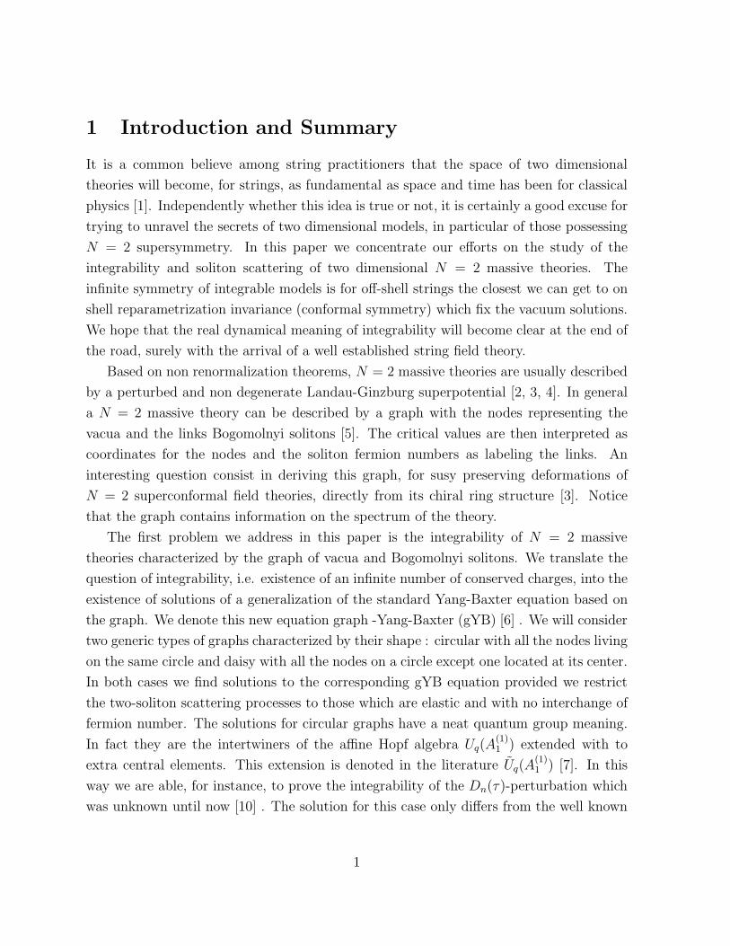
arX

iv:h

ep-t

h/93

1203

2v2

9 D

ec 1

993

On the integrability of N = 2 supersymmetric massive

theories

Cesar Gomez and German Sierra

Instituto de Matematicas y Fısica Fundamental

CSIC, Serrano 123, E–28006 Spain.

December 1993

Abstract

In this paper we propose a criteria to establish the integrability of N = 2 super-

symmetric massive theories. The basic data required are the vacua and the spectrum

of Bogomolnyi solitons, which can be neatly encoded in a graph (nodes=vacua and

links= Bogomolnyi solitons). Integrability is then equivalent to the existence of

solutions of a generalized Yang-Baxter equation which is built up from the graph

( graph-Yang-Baxter equation). We solve this equation for two general types of

graphs: circular and daisy, proving, in particular, the integrability of the follow-

ing Landau-Ginzburg superpotentials: An(t1), An(t2), Dn(τ), E6(t7), and E8(t16).

For circular graphs the solution are intertwiners of the affine Hopf algebra Uq(A(1)1 ),

while for daisy graphs the solution corresponds to a susy generalization of the Boltz-

mann weights of the chiral Potts model in the trigonometric regime. A chiral Potts

like solution is conjectured for the more tricky case Dn(t2). The scattering theory of

circular models, for instance An(t1) or Dn(τ), is Toda like. The physical spectrum

of daisy models, as An(t2), E6(t7) or E8(t16), is given by confined states of radial

solitons. The scattering theory of the confined states is again Toda like. Bootstrap

factors for the confined solitons are given by fusing the susy chiral Potts S−matrices

of the elementary constituents; i.e the radial solitons of the daisy graph.

0

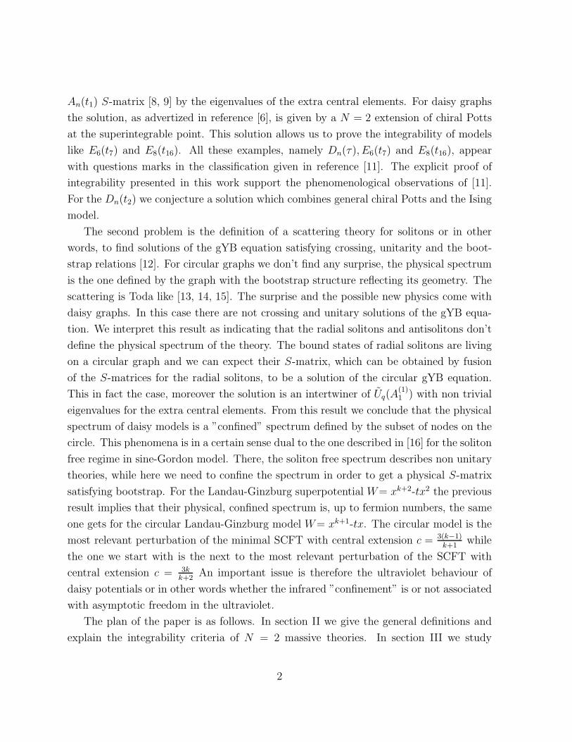
1 Introduction and Summary

It is a common believe among string practitioners that the space of two dimensional

theories will become, for strings, as fundamental as space and time has been for classical

physics [1]. Independently whether this idea is true or not, it is certainly a good excuse for

trying to unravel the secrets of two dimensional models, in particular of those possessing

N = 2 supersymmetry. In this paper we concentrate our efforts on the study of the

integrability and soliton scattering of two dimensional N = 2 massive theories. The

infinite symmetry of integrable models is for off-shell strings the closest we can get to on

shell reparametrization invariance (conformal symmetry) which fix the vacuum solutions.

We hope that the real dynamical meaning of integrability will become clear at the end of

the road, surely with the arrival of a well established string field theory.

Based on non renormalization theorems, N = 2 massive theories are usually described

by a perturbed and non degenerate Landau-Ginzburg superpotential [2, 3, 4]. In general

a N = 2 massive theory can be described by a graph with the nodes representing the

vacua and the links Bogomolnyi solitons [5]. The critical values are then interpreted as

coordinates for the nodes and the soliton fermion numbers as labeling the links. An

interesting question consist in deriving this graph, for susy preserving deformations of

N = 2 superconformal field theories, directly from its chiral ring structure [3]. Notice

that the graph contains information on the spectrum of the theory.

The first problem we address in this paper is the integrability of N = 2 massive

theories characterized by the graph of vacua and Bogomolnyi solitons. We translate the

question of integrability, i.e. existence of an infinite number of conserved charges, into the

existence of solutions of a generalization of the standard Yang-Baxter equation based on

the graph. We denote this new equation graph -Yang-Baxter (gYB) [6] . We will consider

two generic types of graphs characterized by their shape : circular with all the nodes living

on the same circle and daisy with all the nodes on a circle except one located at its center.

In both cases we find solutions to the corresponding gYB equation provided we restrict

the two-soliton scattering processes to those which are elastic and with no interchange of

fermion number. The solutions for circular graphs have a neat quantum group meaning.

In fact they are the intertwiners of the affine Hopf algebra Uq(A(1)1 ) extended with to

extra central elements. This extension is denoted in the literature Uq(A(1)1 ) [7]. In this

way we are able, for instance, to prove the integrability of the Dn(τ)-perturbation which

was unknown until now [10] . The solution for this case only differs from the well known

1

An(t1) S-matrix [8, 9] by the eigenvalues of the extra central elements. For daisy graphs

the solution, as advertized in reference [6], is given by a N = 2 extension of chiral Potts

at the superintegrable point. This solution allows us to prove the integrability of models

like E6(t7) and E8(t16). All these examples, namely Dn(τ), E6(t7) and E8(t16), appear

with questions marks in the classification given in reference [11]. The explicit proof of

integrability presented in this work support the phenomenological observations of [11].

For the Dn(t2) we conjecture a solution which combines general chiral Potts and the Ising

model.

The second problem is the definition of a scattering theory for solitons or in other

words, to find solutions of the gYB equation satisfying crossing, unitarity and the boot-

strap relations [12]. For circular graphs we don’t find any surprise, the physical spectrum

is the one defined by the graph with the bootstrap structure reflecting its geometry. The

scattering is Toda like [13, 14, 15]. The surprise and the possible new physics come with

daisy graphs. In this case there are not crossing and unitary solutions of the gYB equa-

tion. We interpret this result as indicating that the radial solitons and antisolitons don’t

define the physical spectrum of the theory. The bound states of radial solitons are living

on a circular graph and we can expect their S-matrix, which can be obtained by fusion

of the S-matrices for the radial solitons, to be a solution of the circular gYB equation.

This in fact the case, moreover the solution is an intertwiner of Uq(A(1)1 ) with non trivial

eigenvalues for the extra central elements. From this result we conclude that the physical

spectrum of daisy models is a ”confined” spectrum defined by the subset of nodes on the

circle. This phenomena is in a certain sense dual to the one described in [16] for the soliton

free regime in sine-Gordon model. There, the soliton free spectrum describes non unitary

theories, while here we need to confine the spectrum in order to get a physical S-matrix

satisfying bootstrap. For the Landau-Ginzburg superpotential W= xk+2-tx2 the previous

result implies that their physical, confined spectrum is, up to fermion numbers, the same

one gets for the circular Landau-Ginzburg model W= xk+1-tx. The circular model is the

most relevant perturbation of the minimal SCFT with central extension c = 3(k−1)k+1

while

the one we start with is the next to the most relevant perturbation of the SCFT with

central extension c = 3kk+2

An important issue is therefore the ultraviolet behaviour of

daisy potentials or in other words whether the infrared ”confinement” is or not associated

with asymptotic freedom in the ultraviolet.

The plan of the paper is as follows. In section II we give the general definitions and

explain the integrability criteria of N = 2 massive theories. In section III we study

2

circular and daisy graphs proving their integrability and aplying the results to some

Landau-Ginzburg models whose integrability was unclear. In section IV we consider the

scattering theory and discuss the confined spectrum for daisy graphs.

2 N=2 massive theories

2.1 Definitions

Let us denote by A the N = 2 algebra:

(Q±)2 = (Q±)2 = {Q+, Q−} = {Q−, Q+} = 0 ,

{Q+, Q−} = P, {Q+, Q−} = P , (1)

{Q+, Q+} = W, {Q−, Q−} = W ,[

F , Q±]

= ±Q±,[

F , Q±]

= ∓Q±

where Q±,Q± are the susy generators, W the topological central term [17] and F the

fermion number. The N = 2 algebra is equipped with a coalgebra structure defined by

the following comultiplication rules:

∆Q± = Q± ⊗ 1 + e±iπF ⊗Q±

∆Q± = Q± ⊗ 1 + e∓iπF ⊗ Q± (2)

∆W = W ⊗ 1 + 1 ⊗W

∆P = P ⊗ 1 + 1 ⊗ P

By a massive theory we mean one with a mass gap and non degenerate vacua. Given a

couple of ordered vacua (i, j) a soliton si,j is a field configuration satisfying the equation of

motion and which connects the vacua i at x = −∞ with the vacua j at x = ∞. Following

the spirit of reference [5] we define a massive N = 2 theory by the following set of data:

D1) A graph G characterized by a set of nodes i, j, .. and positive integer numbers µi,j

which counts the number of links between the nodes i and j.

D2) Complex coordinates wi for the nodes and real numbers fi,j associated with each

ordered couple of connected nodes.

3

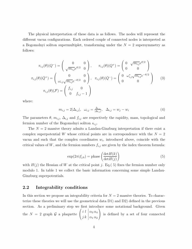
The physical interpretation of these data is as follows. The nodes will represent the

different vacua configurations. Each ordered couple of connected nodes is interpreted as

a Bogomolnyi soliton supermultiplet, transforming under the N = 2 supersymmetry as

follows:

πi,j(θ)(Q−) =

0 0√mi,je

θ/2 0

, πi,j(θ)(Q+) =

0√mi,je

θ/2

0 0

πi,j(θ)(Q+) =

0 0

ωi,j√mi,je

−θ/2 0

, πi,j(θ)(Q−) =

0 ω∗i,j√mi,je

−θ/2

0 0

(3)

πi,j(θ)(F) =

fi,j 0

0 fi,j − 1

where:

mi,j = 2|∆i,j|, ωi,j =∆i,j

|∆i,j |, ∆i,j = wj − wi (4)

The parameters θ, mi,j , ∆i,j and fi,j are respectively the rapidity, mass, topological and

fermion number of the Bogomolnyi soliton si,j.

The N = 2 massive theory admits a Landau-Ginzburg interpretation if there exist a

complex superpotential W whose critical points are in correspondence with the N = 2

vacua and such that the complex coordinates wi, introduced above, coincide with the

critical values of W , and the fermion numbers fi,j are given by the index theorem formula:

exp(2πifj,k) = phase

(

detH(k)

detH(j)

)

(5)

with H(j) the Hessian of W at the critical point j. Eq.( 5) fixes the fermion number only

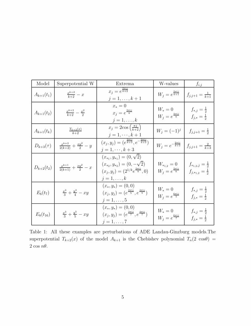
modulo 1. In table 1 we collect the basic information concerning some simple Landau-

Ginzburg superpotentials.

2.2 Integrability conditions

In this section we propose an integrability criteria for N = 2 massive theories. To charac-

terize these theories we will use the geometrical data D1) and D2) defined in the previous

section. As a preliminary step we first introduce some notational background. Given

the N = 2 graph G a plaquette

i l

j k

∣

∣

∣

∣

∣

∣

α3 α4

α1 α2

is defined by a set of four connected

4

Model Superpotential W Extrema W-values fi,j

Ak+1(t1)xk+2

k+2− x

xj = e2πijk+2

j = 1, . . . , k + 1Wj = e

2πijk+1 fj,j+1 = 1

k+1

Ak+1(t2)xk+2

k+2− x2

2

x∗ = 0

xj = e2πijk

j = 1, . . . , k

W∗ = 0

Wj = e4πijk

f∗,j = 12

fj,∗ = 12

Ak+1(tk)Tk+2(x)k+2

xj = 2cos(

πjk+2

)

j = 1, · · · , k + 1Wj = (−1)j fj,j+1 = 1

2

Dk+3(τ)xk+2

2(k+2)+ xy2

2− y

(xj , yj) = (e2πijk+3 , e−

2πijk+3 )

j = 1, · · · , k + 3Wj = e−

2πijk+3 fj,j+1 = 2

k+3

Dk+2(t2)xk+1

2(k+1)+ xy2

2− x

(x∗1, y∗1

) = (0,√

2)

(x∗2, y∗2

) = (0,−√

2)

(xj , yj) = (21/ke2πijk , 0)

j = 1, . . . , k

W∗1,2 = 0

Wj = e2πijk

f∗1,2,j = 12

fj,∗1,2 = 12

E6(t7)x3

3+ y4

4− xy

(x∗, y∗) = (0, 0)

(xj , yj) = (e2πij

5 , e4πij

5 )

j = 1, . . . , 5

W∗ = 0

Wj = e6πij

5

f∗,j = 12

fj,∗ = 12

E8(t16)x3

3+ y5

5− xy

(x∗, y∗) = (0, 0)

(xj , yj) = (e2πij

7 , e4πij

7 )

j = 1, . . . , 7

W∗ = 0

Wj = e6πij

7

f∗,j = 12

fj,∗ = 12

Table 1: All these examples are perturbations of ADE Landau-Ginzburg models.The

superpotential Tk+2(x) of the model Ak+1 is the Chebishev polynomial Tn(2 cosθ) =

2 cos nθ.

5

✉

✉ ✉

✉

i

j k

l

α1

α2

α3

α4

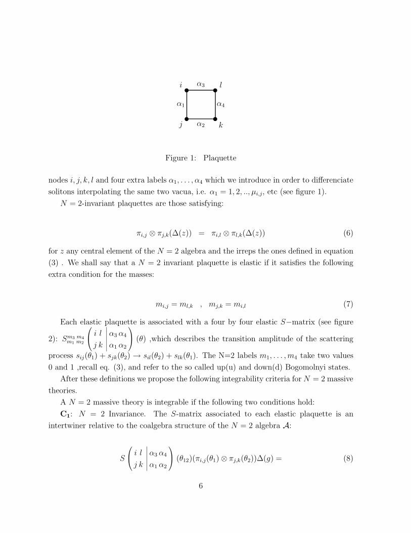
Figure 1: Plaquette

nodes i, j, k, l and four extra labels α1, . . . , α4 which we introduce in order to differenciate

solitons interpolating the same two vacua, i.e. α1 = 1, 2, .., µi,j, etc (see figure 1).

N = 2-invariant plaquettes are those satisfying:

πi,j ⊗ πj,k(∆(z)) = πi,l ⊗ πl,k(∆(z)) (6)

for z any central element of the N = 2 algebra and the irreps the ones defined in equation

(3) . We shall say that a N = 2 invariant plaquette is elastic if it satisfies the following

extra condition for the masses:

mi,j = ml,k , mj,k = mi,l (7)

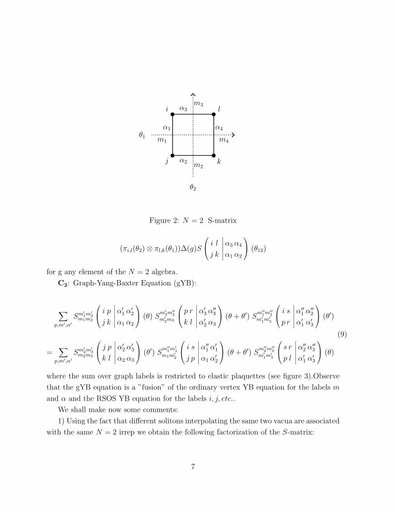
Each elastic plaquette is associated with a four by four elastic S−matrix (see figure

2): Sm3 m4

m1 m2

i l

j k

∣

∣

∣

∣

∣

∣

α3 α4

α1 α2

(θ) ,which describes the transition amplitude of the scattering

process sij(θ1) + sjk(θ2) → sil(θ2) + slk(θ1). The N=2 labels m1, . . . , m4 take two values

0 and 1 ,recall eq. (3), and refer to the so called up(u) and down(d) Bogomolnyi states.

After these definitions we propose the following integrability criteria forN = 2 massive

theories.

A N = 2 massive theory is integrable if the following two conditions hold:

C1: N = 2 Invariance. The S-matrix associated to each elastic plaquette is an

intertwiner relative to the coalgebra structure of the N = 2 algebra A:

S

i l

j k

∣

∣

∣

∣

∣

∣

α3 α4

α1 α2

(θ12)(πi,j(θ1) ⊗ πj,k(θ2))∆(g) = (8)

6

✉ ✉

✉✉i

j k

l

α1

α2

α3

α4

θ1

θ2

m1 m4

m2

m3

Figure 2: N = 2 S-matrix

(πi,l(θ2) ⊗ πl,k(θ1))∆(g)S

i l

j k

∣

∣

∣

∣

∣

∣

α3 α4

α1 α2

(θ12)

for g any element of the N = 2 algebra.

C2: Graph-Yang-Baxter Equation (gYB):

∑

p,m′,α′

Sm′

1m′

2m1m2

i p

j k

∣

∣

∣

∣

∣

∣

α′1 α

′2

α1 α2

(θ) Sm′

3m′′

3

m′

2m3

p r

k l

∣

∣

∣

∣

∣

∣

α′3 α

′′3

α′2 α3

(θ + θ′) Sm′′

1m′′

2

m′

1m′

3

i s

p r

∣

∣

∣

∣

∣

∣

α′′1 α

′′2

α′1 α

′3

(θ′)

(9)

=∑

p,m′,α′

Sm′

2m′

3m2m3

j p

k l

∣

∣

∣

∣

∣

∣

α′2 α

′3

α2 α3

(θ′) Sm′′

1m′

1

m1m′

2

i s

j p

∣

∣

∣

∣

∣

∣

α′′1 α

′1

α1 α′2

(θ + θ′) Sm′′

2m′′

3

m′

1m′

3

s r

p l

∣

∣

∣

∣

∣

∣

α′′2 α

′′3

α′1 α

′3

(θ)

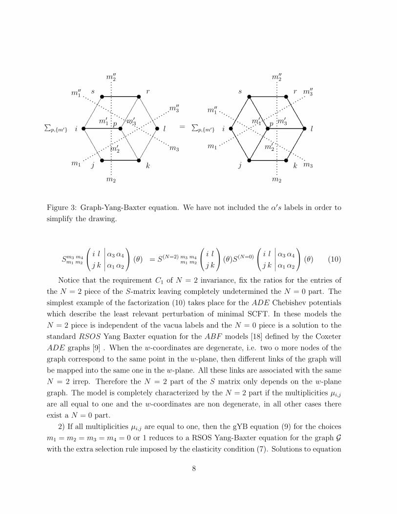
where the sum over graph labels is restricted to elastic plaquettes (see figure 3).Observe

that the gYB equation is a ”fusion” of the ordinary vertex YB equation for the labels m

and α and the RSOS YB equation for the labels i, j, etc..

We shall make now some comments:

1) Using the fact that different solitons interpolating the same two vacua are associated

with the same N = 2 irrep we obtain the following factorization of the S-matrix:

7

✔✔✔✔✔✔

✔✔

✔✔

❚❚❚❚❚❚

❚❚

❚❚

❚❚❚❚❚✔

✔✔

✔✔

✉

✉✉

✉

✉ ✉

✉ ❚❚

❚❚

❚❚❚❚❚❚✔

✔✔

✔✔ ✔

✔✔✔✔

✔✔

✔✔

✔❚❚❚❚❚

✉ ✉

✉✉

✉

✉ ✉

i i

j j

s s

p

k k

l l

r r

p=∑

p,{m′}

∑

p,{m′}

m1

m2

m3

m′′3

m′′2

m′′1

m′1

m′2

m′3

m1

m2

m3

m′′1

m′′2

m′′3

m′1

m′2

m′3

Figure 3: Graph-Yang-Baxter equation. We have not included the α′s labels in order to

simplify the drawing.

Sm3 m4

m1 m2

i l

j k

∣

∣

∣

∣

∣

∣

α3 α4

α1 α2

(θ) = S(N=2) m3 m4

m1 m2

i l

j k

(θ)S(N=0)

i l

j k

∣

∣

∣

∣

∣

∣

α3 α4

α1 α2

(θ) (10)

Notice that the requirement C1 of N = 2 invariance, fix the ratios for the entries of

the N = 2 piece of the S-matrix leaving completely undetermined the N = 0 part. The

simplest example of the factorization (10) takes place for the ADE Chebishev potentials

which describe the least relevant perturbation of minimal SCFT. In these models the

N = 2 piece is independent of the vacua labels and the N = 0 piece is a solution to the

standard RSOS Yang Baxter equation for the ABF models [18] defined by the Coxeter

ADE graphs [9] . When the w-coordinates are degenerate, i.e. two o more nodes of the

graph correspond to the same point in the w-plane, then different links of the graph will

be mapped into the same one in the w-plane. All these links are associated with the same

N = 2 irrep. Therefore the N = 2 part of the S matrix only depends on the w-plane

graph. The model is completely characterized by the N = 2 part if the multiplicities µi,j

are all equal to one and the w-coordinates are non degenerate, in all other cases there

exist a N = 0 part.

2) If all multiplicities µi,j are equal to one, then the gYB equation (9) for the choices

m1 = m2 = m3 = m4 = 0 or 1 reduces to a RSOS Yang-Baxter equation for the graph Gwith the extra selection rule imposed by the elasticity condition (7). Solutions to equation

8

(8) and to the full fledged gYB equation (9) would be equivalent, in these cases, to the

existence of a N = 2 supersymmetric extension of the corresponding RSOS statistical

model.

3) The N = 2 massive theories can possess, in some particular cases, extra N = 0

symmetries that would impose additional restrictions on the N = 0 part of the S-matrix.

The N = 0 symmetry, if present, will act on the multiplicity labels (α) fixing the ratios for

the different entries of the N = 0 S-matrix. This N = 0 symmetry can be associated with

a classical or a quantum algebra and in all cases commute with the N = 2 supersymmetry.

CP n sigma models and affine perturbations of Kazama-Suzuki cosets are good examples

of N = 2 massive theories with N = 0 symmetries.

4) Extra integrability symmetries. A possible scenario we will often find is that of

N = 2 massive theories where the gYB equation has not solution, unless we restrict the

set of elastic plaquettes. Of course this restriction should not imply the restriction of the

graph, i.e. the physical decoupling of any vacua. If this is the case we would conclude that

the theory is integrable and that the extra selection rule is an integrability symmetry. In

all the integrable N = 2 massive theories we have studied, integrability is obtained after

reducing the elastic plaquettes to those with equal fermion numbers for opposite sides and

therefore the fermion number appears as an ”individual” conserved quantity. In principle,

this extra selection rule is independent of the general Z-invariance [19] which underlines

integrability.

5) The integrability of the N = 2 massive theories, characterized by conditions C1

and C2 should not be confussed with the existence of a well defined scattering theory. As

we will discuss in section IV in order to define a scattering theory we need to impose the

additional physical requirements of unitarity, crossing and bootstrap.

6) The geometrical data D1 and D2 we have used to define a massive N = 2 theory,

together with the conditions C1 and C2 in terms of which we characterize its integrability,

can be interpreted from a mathematical point of view, as a way to define a new math-

ematical structure which generalizes that of quantum groups. This new mathematical

object or, graph quantum group, would be defined by a Hopf algebra A, a graph, and a

map from links of the graph into irreps of the Hopf algebra in such a way that for any

plaquette of the graph there exist an intertwiner satisfying conditions C1 and C2. The

main difference with respect to ordinary quantum groups is that now the intertwiner sta-

blish an equivalence between irreps which are not necessarily related by a permutation.

Therefore these intertwiners cannot follow from a universal R-matrix.

9

✜✜

✜✜

❊❊❊❊❊❍❍❍❍❍

✟✟✟✟✟☎☎☎☎☎

❭❭

❭❭

① ①

①

①

①

①

①①

❈❈❈

❅❅

❳❳❳✘✘✘�

�✄✄✄❈❈❈❅❅❳❳❳✘✘✘�

�✄✄✄①

①

①①

①

①

①

①

①①

①

①

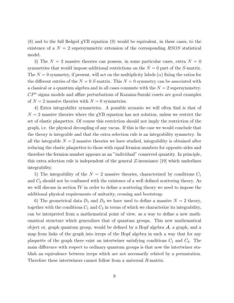
Figure 4: Circular and daisy graphs

3 Partial Classification of Integrable N = 2 Massive

Theories

In this section we present a partial classification of integrable N = 2 theories, mostly

based on the geometry of the graph. We consider two basic types of geometries, which

seem to be the basic building blocks of most of the known soliton polytopes [15] , namely

circular graphs with all the nodes on the same circle and daisy graphs with all nodes on

the same circle except one which is located at the center (see fig. 4).

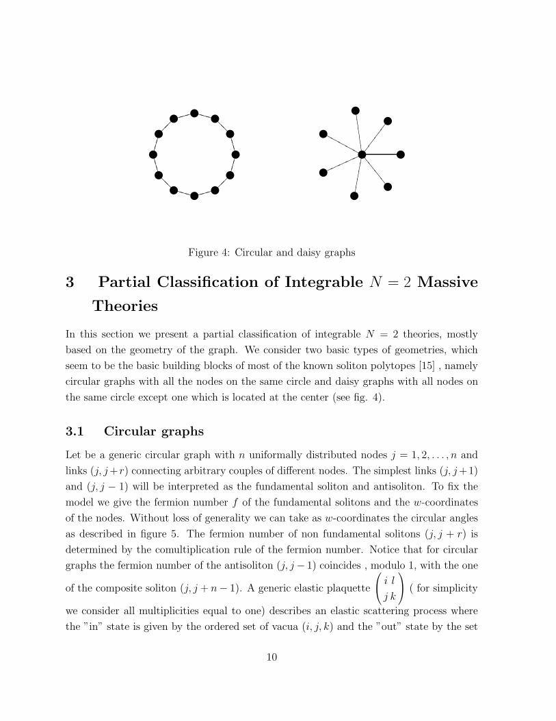
3.1 Circular graphs

Let be a generic circular graph with n uniformally distributed nodes j = 1, 2, . . . , n and

links (j, j+r) connecting arbitrary couples of different nodes. The simplest links (j, j+1)

and (j, j − 1) will be interpreted as the fundamental soliton and antisoliton. To fix the

model we give the fermion number f of the fundamental solitons and the w-coordinates

of the nodes. Without loss of generality we can take as w-coordinates the circular angles

as described in figure 5. The fermion number of non fundamental solitons (j, j + r) is

determined by the comultiplication rule of the fermion number. Notice that for circular

graphs the fermion number of the antisoliton (j, j− 1) coincides , modulo 1, with the one

of the composite soliton (j, j + n− 1). A generic elastic plaquette

i l

j k

( for simplicity

we consider all multiplicities equal to one) describes an elastic scattering process where

the ”in” state is given by the ordered set of vacua (i, j, k) and the ”out” state by the set

10

❅❅

❅✏✏✏✏✏✏✏✏✏ PPPPPPPPP��

�→2ψ1

2ψ2 2ψ12ψ2①

①

① ①

①

①wi wi

wj wl

wk wk

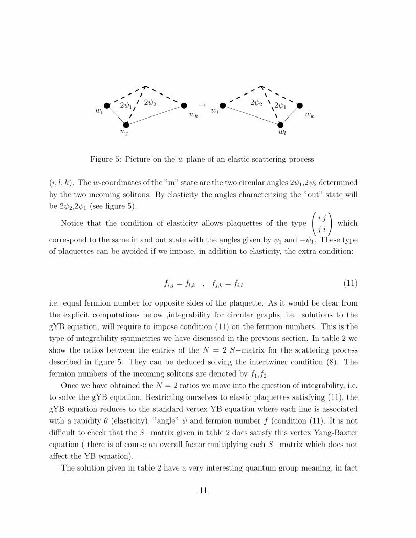
Figure 5: Picture on the w plane of an elastic scattering process

(i, l, k). The w-coordinates of the ”in” state are the two circular angles 2ψ1,2ψ2 determined

by the two incoming solitons. By elasticity the angles characterizing the ”out” state will

be 2ψ2,2ψ1 (see figure 5).

Notice that the condition of elasticity allows plaquettes of the type

i j

j i

which

correspond to the same in and out state with the angles given by ψ1 and −ψ1. These type

of plaquettes can be avoided if we impose, in addition to elasticity, the extra condition:

fi,j = fl,k , fj,k = fi,l (11)

i.e. equal fermion number for opposite sides of the plaquette. As it would be clear from

the explicit computations below ,integrability for circular graphs, i.e. solutions to the

gYB equation, will require to impose condition (11) on the fermion numbers. This is the

type of integrability symmetries we have discussed in the previous section. In table 2 we

show the ratios between the entries of the N = 2 S−matrix for the scattering process

described in figure 5. They can be deduced solving the intertwiner condition (8). The

fermion numbers of the incoming solitons are denoted by f1,f2.

Once we have obtained the N = 2 ratios we move into the question of integrability, i.e.

to solve the gYB equation. Restricting ourselves to elastic plaquettes satisfying (11), the

gYB equation reduces to the standard vertex YB equation where each line is associated

with a rapidity θ (elasticity), ”angle” ψ and fermion number f (condition (11). It is not

difficult to check that the S−matrix given in table 2 does satisfy this vertex Yang-Baxter

equation ( there is of course an overall factor multiplying each S−matrix which does not

affect the YB equation).

The solution given in table 2 have a very interesting quantum group meaning, in fact

11

m3 m4

m1 m2

Sm3 m4

m1 m2(ψ1, ψ2)/S

0 00 0(ψ1, ψ2)

1 1

1 1−eiπ(f1−f2)ei(ψ2−ψ1) sinh( θ

2−i

ψ1+ψ22

)

sinh( θ2+i

ψ1+ψ22

)

1 0

0 1eiπf1e−iψ1

sinh( θ2−i

ψ1−ψ22

)

sinh( θ2+i

ψ1+ψ22

)

0 1

1 0e−iπf2eiψ2

sinh( θ2+i

ψ1−ψ22

)

sinh( θ2+i

ψ1+ψ22

)

0 1

0 1ieiπ(f1−f2)e−i

ψ1−ψ22

(sinψ1sinψ2)1/2

sinh( θ2+i

ψ1+ψ22

)

1 0

1 0ie−i

ψ1−ψ22

(sinψ1sinψ2)1/2

sinh( θ2+i

ψ1+ψ22

)

Table 2: Relations imposed by the N=2 intertwiner condition on ”circular” S−matrices.

it is the quantum R-matrix intertwiner for the Hopf algebra Uq(A(1)1 ) with deformation

parameter q4 = 1. This Hopf algebra, which was introduced in reference [7], is very

close to the Hopf algebra Uq(A(1)1 ). The only changes are the addition of two new central

elements Zi(i = 0, 1) which modify the usual comultiplication rules of the rest of the

elements of Uq(A(1)1 ) as follows :

∆Ei = Ei ⊗ 1 + Zi Ki ⊗ Ei

∆Fi = Fi ⊗K−1i + Z−1

i ⊗ Fi (12)

∆Ki = Ki ⊗Ki

∆Zi = Zi ⊗ Zi

We shall be interested in the so called nilpotent representations [20] of the Uq(A(1)1 )

algebra which are labelled, in addition to the rapidity θ, by a pair ξ = (λ, z) of non zero

complex numbers. They are given by:

πλ,z(θ)(E0) = d(λ)

0 0

eθ/2 0

, πλ,z(θ)(E1) = d(λ)

0 eθ/2

0 0

12

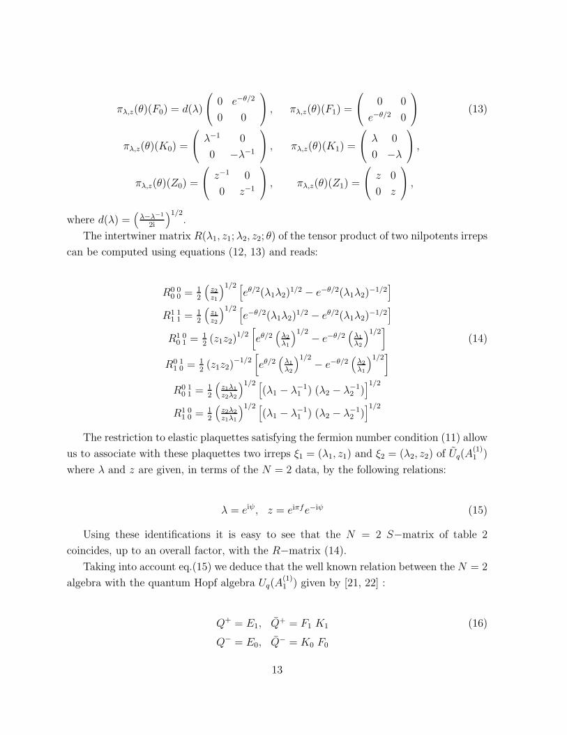
πλ,z(θ)(F0) = d(λ)

0 e−θ/2

0 0

, πλ,z(θ)(F1) =

0 0

e−θ/2 0

(13)

πλ,z(θ)(K0) =

λ−1 0

0 −λ−1

, πλ,z(θ)(K1) =

λ 0

0 −λ

,

πλ,z(θ)(Z0) =

z−1 0

0 z−1

, πλ,z(θ)(Z1) =

z 0

0 z

,

where d(λ) =(

λ−λ−1

2i

)1/2.

The intertwiner matrix R(λ1, z1;λ2, z2; θ) of the tensor product of two nilpotents irreps

can be computed using equations (12, 13) and reads:

R0 00 0 = 1

2

(

z2z1

)1/2 [

eθ/2(λ1λ2)1/2 − e−θ/2(λ1λ2)

−1/2]

R1 11 1 = 1

2

(

z1z2

)1/2 [

e−θ/2(λ1λ2)1/2 − eθ/2(λ1λ2)

−1/2]

R1 00 1 = 1

2(z1z2)

1/2[

eθ/2(

λ2

λ1

)1/2 − e−θ/2(

λ1

λ2

)1/2]

(14)

R0 11 0 = 1

2(z1z2)

−1/2[

eθ/2(

λ1

λ2

)1/2 − e−θ/2(

λ2

λ1

)1/2]

R0 10 1 = 1

2

(

z1λ1

z2λ2

)1/2 [

(λ1 − λ−11 ) (λ2 − λ−1

2 )]1/2

R1 01 0 = 1

2

(

z2λ2

z1λ1

)1/2 [

(λ1 − λ−11 ) (λ2 − λ−1

2 )]1/2

The restriction to elastic plaquettes satisfying the fermion number condition (11) allow

us to associate with these plaquettes two irreps ξ1 = (λ1, z1) and ξ2 = (λ2, z2) of Uq(A(1)1 )

where λ and z are given, in terms of the N = 2 data, by the following relations:

λ = eiψ, z = eiπfe−iψ (15)

Using these identifications it is easy to see that the N = 2 S−matrix of table 2

coincides, up to an overall factor, with the R−matrix (14).

Taking into account eq.(15) we deduce that the well known relation between the N = 2

algebra with the quantum Hopf algebra Uq(A(1)1 ) given by [21, 22] :

Q+ = E1, Q+ = F1 K1 (16)

Q− = E0, Q− = K0 F0

13

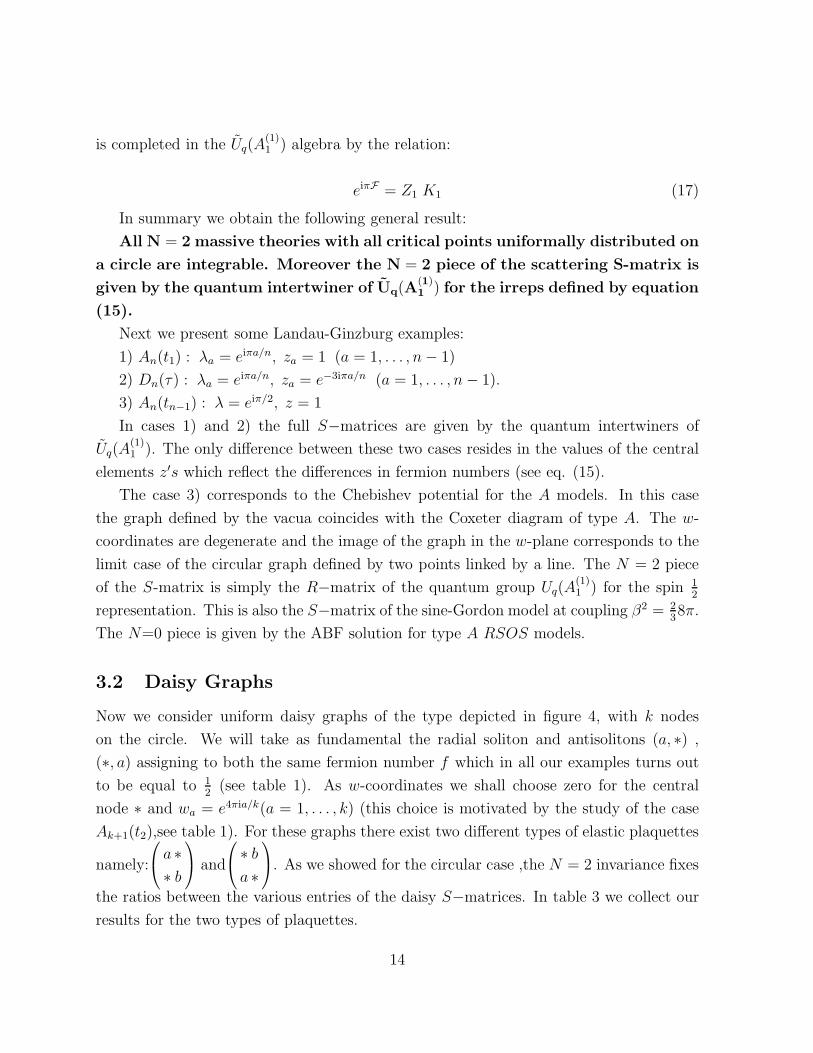
is completed in the Uq(A(1)1 ) algebra by the relation:

eiπF = Z1 K1 (17)

In summary we obtain the following general result:

All N = 2 massive theories with all critical points uniformally distributed on

a circle are integrable. Moreover the N = 2 piece of the scattering S-matrix is

given by the quantum intertwiner of Uq(A(1)1 ) for the irreps defined by equation

(15).

Next we present some Landau-Ginzburg examples:

1) An(t1) : λa = eiπa/n, za = 1 (a = 1, . . . , n− 1)

2) Dn(τ) : λa = eiπa/n, za = e−3iπa/n (a = 1, . . . , n− 1).

3) An(tn−1) : λ = eiπ/2, z = 1

In cases 1) and 2) the full S−matrices are given by the quantum intertwiners of

Uq(A(1)1 ). The only difference between these two cases resides in the values of the central

elements z′s which reflect the differences in fermion numbers (see eq. (15).

The case 3) corresponds to the Chebishev potential for the A models. In this case

the graph defined by the vacua coincides with the Coxeter diagram of type A. The w-

coordinates are degenerate and the image of the graph in the w-plane corresponds to the

limit case of the circular graph defined by two points linked by a line. The N = 2 piece

of the S-matrix is simply the R−matrix of the quantum group Uq(A(1)1 ) for the spin 1

2

representation. This is also the S−matrix of the sine-Gordon model at coupling β2 = 238π.

The N=0 piece is given by the ABF solution for type A RSOS models.

3.2 Daisy Graphs

Now we consider uniform daisy graphs of the type depicted in figure 4, with k nodes

on the circle. We will take as fundamental the radial soliton and antisolitons (a, ∗) ,

(∗, a) assigning to both the same fermion number f which in all our examples turns out

to be equal to 12

(see table 1). As w-coordinates we shall choose zero for the central

node ∗ and wa = e4πia/k(a = 1, . . . , k) (this choice is motivated by the study of the case

Ak+1(t2),see table 1). For these graphs there exist two different types of elastic plaquettes

namely:

a ∗∗ b

and

∗ ba ∗

. As we showed for the circular case ,the N = 2 invariance fixes

the ratios between the various entries of the daisy S−matrices. In table 3 we collect our

results for the two types of plaquettes.

14

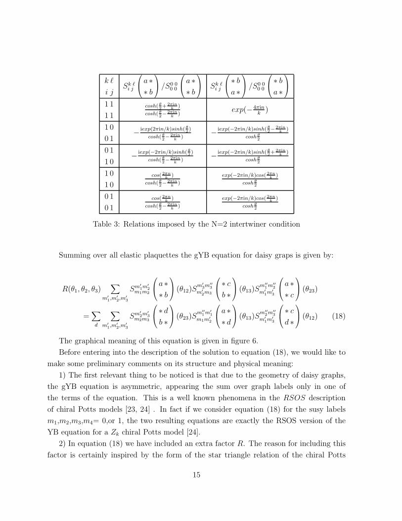
k ℓ

i jSk ℓi j

a ∗∗ b

/S0 00 0

a ∗∗ b

Sk ℓi j

∗ ba ∗

/S0 00 0

∗ ba ∗

1 1

1 1

cosh( θ2+ 2πin

k)

cosh( θ2− 2πin

k)

exp(−4πink

)

1 0

0 1− iexp(2πin/k)sinh( θ

2)

cosh( θ2− 2πin

k)

− iexp(−2πin/k)sinh( θ2− 2πin

k)

cosh θ2

0 1

1 0− iexp(−2πin/k)sinh( θ

2)

cosh( θ2− 2πin

k)

− iexp(−2πin/k)sinh( θ2+ 2πin

k)

cosh θ2

1 0

1 0

cos( 2πnk

)

cosh( θ2− 2πin

k)

exp(−2πin/k)cos( 2πnk

)

cosh θ2

0 1

0 1

cos( 2πnk

)

cosh( θ2− 2πin

k)

exp(−2πin/k)cos( 2πnk

)

cosh θ2

Table 3: Relations imposed by the N=2 intertwiner condition

Summing over all elastic plaquettes the gYB equation for daisy graps is given by:

R(θ1, θ2, θ3)∑

m′

1,m′

2,m′

3

Sm′

1m′

2m1m2

a ∗∗ b

(θ12)Sm′

3m′′

3

m′

2m3

∗ cb ∗

(θ13)Sm′′

1m′′

2

m′

1m′

3

a ∗∗ c

(θ23)

=∑

d

∑

m′

1,m′

2,m′

3

Sm′

2m′

3m2m3

∗ db ∗

(θ23)Sm′′

1m′

1

m1m′

2

a ∗∗ d

(θ13)Sm′′

2m′′

3

m′

1m′

3

∗ cd ∗

(θ12) (18)

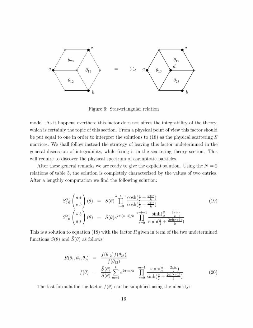
The graphical meaning of this equation is given in figure 6.

Before entering into the description of the solution to equation (18), we would like to

make some preliminary comments on its structure and physical meaning:

1) The first relevant thing to be noticed is that due to the geometry of daisy graphs,

the gYB equation is asymmetric, appearing the sum over graph labels only in one of

the terms of the equation. This is a well known phenomena in the RSOS description

of chiral Potts models [23, 24] . In fact if we consider equation (18) for the susy labels

m1,m2,m3,m4= 0,or 1, the two resulting equations are exactly the RSOS version of the

YB equation for a Zk chiral Potts model [24].

2) In equation (18) we have included an extra factor R. The reason for including this

factor is certainly inspired by the form of the star triangle relation of the chiral Potts

15

✔✔✔✔✔✔

✔✔

✔✔

❚❚❚❚❚❚

❚❚

❚❚

❚❚❚❚❚✔

✔✔

✔✔

θ12

θ23

θ13 θ13

θ23

θ12

∗

✉∗

✉

∗ ✉

∗ ❚❚

❚❚

❚❚❚❚❚❚✔

✔✔

✔✔ ✔

✔✔✔✔

✔✔

✔✔

✔❚❚❚❚❚

✉ ∗

✉∗

✉

∗ ✉

a a

b b

c c

d=∑

d

Figure 6: Star-triangular relation

model. As it happens overthere this factor does not affect the integrability of the theory,

which is certainly the topic of this section. From a physical point of view this factor should

be put equal to one in order to interpret the solutions to (18) as the physical scattering S

matrices. We shall follow instead the strategy of leaving this factor undetermined in the

general discussion of integrability, while fixing it in the scattering theory section. This

will require to discover the physical spectrum of asymptotic particles.

After these general remarks we are ready to give the explicit solution. Using the N = 2

relations of table 3, the solution is completely characterized by the values of two entries.

After a lengthly computation we find the following solution:

S0 00 0

a ∗∗ b

(θ) = S(θ)a−b−1∏

r=0

cosh( θ2

+ 2πirk

)

cosh( θ2− 2πir

k)

(19)

S0 00 0

∗ ba ∗

(θ) = S(θ)e2πi(a−b)/ka−b−1∏

r=0

sinh( θ2− 2πir

k)

sinh( θ2

+ 2πi(r+1)k

)

This is a solution to equation (18) with the factor R given in term of the two undetermined

functions S(θ) and S(θ) as follows:

R(θ1, θ2, θ3) =f(θ12)f(θ23)

f(θ13)

f(θ) =S(θ)

S(θ)

k∑

m=1

e2πim/km−1∏

r=0

sinh( θ2− 2πir

k)

sinh( θ2

+ 2πi(r+1)k

)(20)

The last formula for the factor f(θ) can be simplified using the identity:

16

k∑

m=1

e2πim/km−1∏

r=0

sinh( θ2− 2πir

k)

sinh( θ2

+ 2πi(r+1)k

)=

√ke3πi(k−1)/4

(k−1)/2∏

j=1

cosh(

θ2− 2πij

k

)

sinh(

θ2

+ 2πijk

) (21)

The previous solution (19) have an intrinsic meaning from the point of view of chiral

Potts. In fact the entries S0 00 0 and S11

11 are two different trigonometric solution of the

chiral Potts model characterized by a parameter ω = e4πi/k , ”moduli” k′ = 1 and ”chiral

angles”:

φ =π

2(k ∓ 2), φ =

π

2(k ± 2) for S00

00 (S1111) (22)

Eq (22) suggest some kind of relation with the so called superintegrable chiral Potts

model which corresponds to the values φ = φ = π2

[25]. This model has received much

attention in the past due to its peculiar properties which singularize it among the more

general class of chiral Potts models [26]. The general daisy graph solution we have de-

scribed above can be used to analize the integrability of some Landau-Ginzburg potentials.

Next we describe five different models all of them associated with daisy graphs ( see table

1 for notations).

1) Ak+1(t2), k=odd. This model corresponds exactly to the solution we have just

described.

2) Ak+1(t2), k=even. In this case we find the phenomena of degenerate w−coordinates

as can be seen from the fact that the k critical points xj = e2πij/k(j = 1, . . . , k) are mapped

onto k/2 distinct points Wj = e4πij/k in the w−plane. We can differenciate two different

subcases depending on the parity of k/2. If k/2 is even there are three collinear points in

the w-plane, while if k/2 is odd this situation does not occur. In the later case the N = 2

part of the S−matrices is again given by eqs.(19), which must be supplemented with a

N = 0 piece to take care of the double degeneracy of the vacua in the w−plane. The

case of collinear vacua is more subtle since, as can be seen from table 3, one gets singular

values for some entries of the S−matrices. These singularities are due to the fact that

whenever we have three collinear points a two soliton state is undistinguishable from a

single soliton state (see reference [5]).

3) E6(t7). The solution of this model is the same as the one for A6(t2).

4) E8(t16).The solution of this model is the same as the one for A8(t2).

5) Dk+2(t2). For simplicity we consider the k= odd case. From table 1 we observe

that the graph is actually three dimensional with k nodes on the x plane, all on the same

17

circle and two extra nodes (∗α, α = 1, 2) on the y line. Inspired by the solution to the

daisy models we can conjecture the following factorization of the S-matrices:

Sm3m4

m1m2

a ∗β∗α b

(θ) = Sm3m4

m1m2

a ∗∗ b

(θ) S

⋄ βα ⋄

(θ) (23)

and similarly for the other type of plaquettes. In this factorization the N = 2 part is the

solution for the daisy graph obtained by proyecting on the w-plane. The N = 0 part is

the standard solution for the Ising model at criticality where now the lattice variables are

identified with the labels α, β = 1, 2.

4 Scattering Theory

The question of integrability of a massive N = 2 theory and its reduction to a scattering

theory satisfying bootstrap and factorization are two different but related questions. In

the study of integrability we start with a graph and formally assume that all links of the

graph correspond to real asymptotic particles. In the spirit of this assumption we solve

the gYB equation and interpret the solutions as scattering S matrices. To promote these

solutions, whose existence already implies an infinite number of conserved charges, to a

real scattering S matrix, requires to impose unitarity, crossing and bootstrap. Only after

fulfilling these physical requirements we can be sure that the N = 2 massive theory is

equivalent to a scattering theory satisfying Zamolodchikov’s axiomatics [12] and that the

links of the graph actually represent the real asymptotic particles.

In this section we will define a closed, in the bootstrap sense, scattering theory for

the two general types of N = 2 massive theories we have described until now, namely

those associated with circular and daisy graphs. The results we find are the following. For

circular graphs the scattering theory is obtained by solving bootstrap equations which are

analogous to the ones describing Toda type theories [13, 14, 15] . The case of daisy graphs

is physically more interesting, as can be already expected from the chiral Potts solution.

A consistent scattering theory can be defined only after reducing the physical spectrum

to composite solitons obtained as soliton-antisoliton bound states. The scattering of these

composite solitons is derived from the chiral Potts solution for radial soliton- antisoliton

scattering by a ”fusion” procedure. The resulting scattering theory is again Toda like

of the same type that for the Dn(τ) model, in the sense that the central elements Z1 of

18

Uq(A(1)1 ) take non trivial values. After these introductory remarks we pass to present our

results.

4.1 Circular Scattering: Toda like spectrum

In the circular case the S−matrix is given by the R−matrix (14) up to an overall factor

Z which depends on the irreps λ1, λ2 which one fixes imposing unitarity, crossing and

bootstrap [9]. Let us suposse that there are n vacua equally space on the same circle

j = 1, . . . , n. The value of λ for the soliton (j, j + r) is given by λ = eiπr/n, while we shall

leave the value of z undetermined. Then the S−matrix describing the scattering of the

soliton (j, j + r1) with rapidity θ1 and the soliton (j + r1, j + r1 + r2) with rapidity θ2 is

given by:

S

j j + r2

j + r1 j + r1 + r2

(θ12) =

Zr1, r2(θ12) R(λ1 = eiπr1/n, zr1 ;λ2 = eiπr2/n, zr2 , θ12) (24)

Unitarity implies the equation:

S

j j + r2

j + r1 j + r1 + r2

(θ) S

j j + r1

j + r2 j + r1 + r2

(−θ) = 1 (25)

and crossing:

Zr1, r2(θ) = Zn−r2, r1(iπ − θ) (26)

The analysis of the bootstrap properties of this model leads finally to the following

expresion of Z1,1 ( see reference [9] for details):

Z1,1(θ) = 1

sinh( θ2−iπn )∏∞j=1

Γ2(−θ/2πi+j)Γ(θ/2πi+j+1/n)Γ(θ/2πi+j−1/n)Γ2(θ/2πi+j)Γ(−θ/2πi+j+1/n)Γ(−θ/2πi+j−1/n)

(27)

= 1

sinh( θ2−iπn )exp

(

2i∫∞0

dttsintθ sinh2πt/n

sinh2πt

)

We shall return to this factor in the next subsection.

19

4.2 Daisy Scattering: Confinement like spectrum

The solution (19) to the gYB equation for daisy graphs was fixed up to two undetermined

functions S(θ) and S(θ). We can use this freedom in order to define an unitary and crossing

symmetric S-matrix satisfying at the same time the gYB equation (18) with the factor R

set equal to one. It is easy to check that there is not solution to all these conditions. Let

us show why this happens in more detail. Crossing symmetry is guaranteed if:

Sm3 m4

m1 m2

∗ ba ∗

(θ) = Sm1 m3

m2 m4

a ∗∗ b

(iπ − θ) (28)

where m = 1, 0 for m = 0, 1. This implies in turn the following relation between S(θ) and

S(θ):

S(θ) = i cotanh(θ

2) S(iπ − θ) (29)

Introducing eq.(29) into (20) and using the relation (21) one deduces:

f(θ) f(iπ − θ) = k (30)

which already implies that the factor R cannot be set equal to one in the gYB equation.

Moreover, the unitarity conditions:

S

a ∗∗ b

(θ)S

a ∗∗ b

(−θ) = 1 (31)

∑

b

S

∗ ab ∗

(θ)S

∗ bc ∗

(−θ) = δa,c 1

are incompatible with crossing. The best that can be done is to find solutions which

satisfy unitarity, but violate crossing by a constant and satisfy the gYB equation with

the factor R also a constant. Notice that the violation of crossing and the existence

of the anomalous factor R in the factorization equations, are two related problems. In

fact by crossing we relate the two types of elastic plaquettes, and the missmatch in the

crossing relation show up in the factor R. The physical origin of these problems can be

partially understood as a consequence of the special symmetry properties of the chiral

Potts Boltzmann weights. In fact the solution (19) is neither P nor T invariant, however

it satisfies the most general requirement of PCT invariance:

20

a− b 0 1 2

S0 00 0

a ∗∗ b

S(θ) S(θ) S(θ)cosh( θ2+ 2πi

3 )cosh( θ2−

2πi

3 )

S1 11 1

a ∗∗ b

S(θ) S(θ)cosh( θ2+ 2πi

3 )cosh( θ2−

2πi

3 )S(θ)

S0 00 0

∗ ba ∗

S(θ) S(θ)e2πi/3sinh θ

2

sinh( θ2+ 2πi

3 )S(θ)

e−2πi/3sinh θ2

sinh( θ2+ 2πi

3 )

S1 11 1

∗ ba ∗

S(θ) S(θ)e−2πi/3sinh θ

2

sinh( θ2+ 2πi

3 )S(θ)

e2πi/3sinh θ2

sinh( θ2+ 2πi

3 )

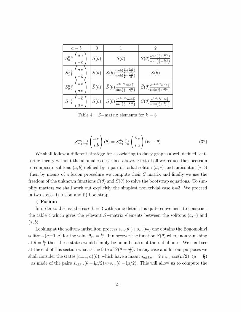
Table 4: S−matrix elements for k = 3

Sm3 m4

m1 m2

a ∗∗ b

(θ) = Sm2 m1

m4 m3

b ∗∗ a

(iπ − θ) (32)

We shall follow a different strategy for associating to daisy graphs a well defined scat-

tering theory without the anomalies described above. First of all we reduce the spectrum

to composite solitons (a, b) defined by a pair of radial soliton (a, ∗) and antisoliton (∗, b),then by means of a fusion procedure we compute their S matrix and finally we use the

freedom of the unknown functions S(θ) and S(θ) to solve the bootstrap equations. To sim-

plify matters we shall work out explicitly the simplest non trivial case k=3. We proceed

in two steps: i) fusion and ii) bootstrap.

i) Fusion:

In order to discuss the case k = 3 with some detail it is quite convenient to construct

the table 4 which gives the relevant S−matrix elements between the solitons (a, ∗) and

(∗, b).Looking at the soliton-antisoliton process sa,∗(θ1)+s∗,b(θ2) one obtains the Bogomolnyi

solitons (a±1, a) for the value θ12 = iπ3. If moreover the function S(θ) where non vanishing

at θ = iπ3

then these states would simply be bound states of the radial ones. We shall see

at the end of this section what is the fate of S(θ = iπ3). In any case and for our purposes we

shall consider the states (a±1, a)(θ), which have a massma±1,a = 2 m∗,a cos(µ/2) (µ = π3)

, as made of the pairs sa±1,∗(θ+ iµ/2)⊗ s∗,a(θ− iµ/2). This will allow us to compute the

21

① ①

①①

θ

θ

θ

θ + iµ

θ − iµ

=∑

b ∗ ∗

∗

∗

a± 1 a

a a∓ 1

a± 1 a

a a∓ 1

b

① ①

①①

①

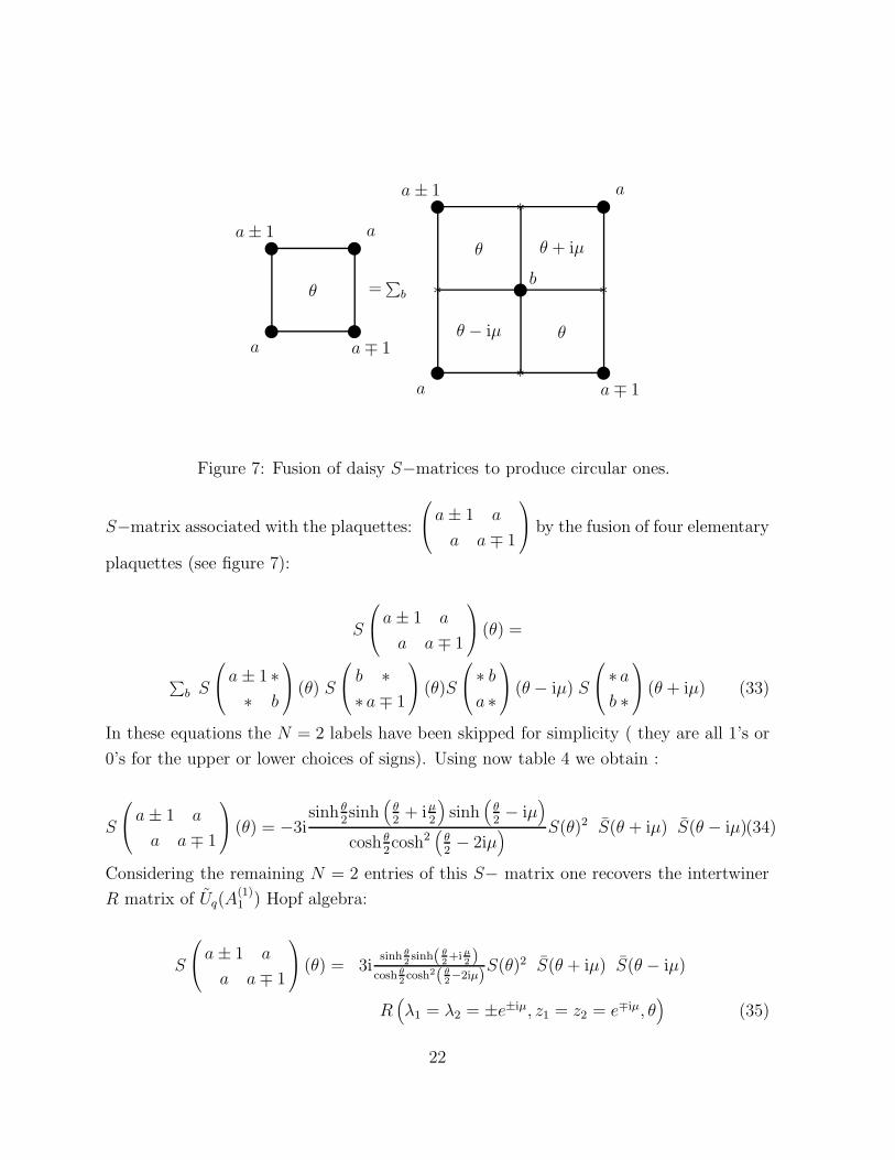
Figure 7: Fusion of daisy S−matrices to produce circular ones.

S−matrix associated with the plaquettes:

a± 1 a

a a∓ 1

by the fusion of four elementary

plaquettes (see figure 7):

S

a± 1 a

a a∓ 1

(θ) =

∑

b S

a± 1 ∗∗ b

(θ) S

b ∗∗ a∓ 1

(θ)S

∗ ba ∗

(θ − iµ) S

∗ ab ∗

(θ + iµ) (33)

In these equations the N = 2 labels have been skipped for simplicity ( they are all 1’s or

0’s for the upper or lower choices of signs). Using now table 4 we obtain :

S

a± 1 a

a a∓ 1

(θ) = −3isinh θ

2sinh

(

θ2

+ iµ2

)

sinh(

θ2− iµ

)

cosh θ2cosh2

(

θ2− 2iµ

) S(θ)2 S(θ + iµ) S(θ − iµ)(34)

Considering the remaining N = 2 entries of this S− matrix one recovers the intertwiner

R matrix of Uq(A(1)1 ) Hopf algebra:

S

a± 1 a

a a∓ 1

(θ) = 3isinh θ

2sinh( θ2+iµ

2 )cosh θ

2cosh2( θ2−2iµ)

S(θ)2 S(θ + iµ) S(θ − iµ)

R(

λ1 = λ2 = ±e±iµ, z1 = z2 = e∓iµ, θ)

(35)

22

The overall factor which depends on S(θ) and S(θ) will be fix by bootstrap. The fused

S matrix satisfies the gYB equation for the circular graph defined by the subset of nodes,

of the daisy graph, in this particular case three, living on the circle. The fusion procedure

we have used able us to get rid of the unpleasent R factors which obscure the physics of

the model.

ii) Bootstrap

Our next step will be to fix the overall factors by imposing crossing, unitarity and

bootstrap on the fused scattering S− matrix. The geometry of the graph and the depen-

dence of this overall factor on the undetermined functions S(θ) and S(θ) suggest already

the answer, namely the bootstrap factors of circular graphs. It is rather amusing and

interesting to observe that the structure of the bootstrap factors Z1,1 = Z2,2 for circular

graphs (27) agrees with the one obtained in (35) by fusion, provided we make the following

identification:

Z1,1(θ) = −3isinh θ

2cosh

(

θ2

+ iπ6

)

cosh(

θ2− iπ

6

)

cosh θ2cosh2

(

θ2− 2πi

3

)

sinh(

θ2− iπ

6

)S(θ)2 S(2πi

3− θ) S(

4πi

3− θ) (36)

From the equation (27) we finally get the following expresion of S(θ):

S(θ) = Ccosh

(

θ2− 2πi

3

)

(

sinh 3θ2

)1/2

∞∏

j=1

Γ(

θ2πi

+ j + 13

)

Γ(

θ2πi

+ j − 13

)

Γ(

− θ2πi

+ j + 13

)

Γ(

− θ2πi

+ j − 13

) (37)

where C is some constant. Strictely speaking eq.(37) is formal since the infinite produc-

torium is actually divergent!. This divergency actually cancells out in equation (36) when

reproducing Z1,1 from S(θ). All these considerations provide a certain amount of evidence

for interpreting the radial solitons as elementary constituents and the physical particles

of daisy graph models as composite solitons. With respect to this second point we should

make the following remark. From relations (37) we get the explicit value of the function

S(θ) , this function have a zero at the value θ = iπ3

(not taking into account the diver-

gence mention above) and therefore the composite state (a±1, a) cannot be taken ”sensu

stricto” as a bound state of two radial solitons. This can be interpreted as reflecting some

kind of confinement of the radial solitons i.e. that they cannot appear as real asymptotic

particles.

To finish this section we would like to make a comment on the possible scattering

theory for the Dk+2(t2) model. Fusing the tentative solution conjectured in equation

23

(23) we can obtain the scattering matrices for a confined spectrum containing now two

different types of composite solitons namely (a, ∗α, b) for α = 1, 2. These S matrices are

the product of a N = 0 part obtained by fusing the Ising components and the same N = 2

part that for the Ak+1(t2).

The physical picture that emerges from the previous analysis of the daisy graph scat-

tering is quite intriging and certainly deserves a deeper study.

Acknowledgements: This work has been supported by the spanish grant n PB92-

1092.

24

References

[1] A.B.Zamolodchikov, JETP Lett. 46 (1987) 160.

V.A.Fateev and A.B.Zamolodchikov, in ”Physics and Mathematics of strings”, World

Scientific (1990) p.245.

[2] C.Vafa and N.P.Warner, Phys.Lett.B218 (1989) 51.

E.Martinec,Phys.Lett.B217 (1989) 431.

[3] W.Lerche,C.Vafa and N.P.Warner,Nucl.Phys.B324 (1989) 427.

[4] N. Warner, Proc.1992 Trieste Summer School.

[5] S.Cecotti and C.Vafa, Nucl.Phys. B367 (1991) 359, ”On the classification of N=2

SUSY theories”, Harvard preprint HUPT-92/A064,SISSA-203/92/EP.

[6] C.Gomez and G.Sierra, CERN-TH.6963/93;UGVA 07/622/93 to appear in

Phys.Lett.

[7] E.Date, M.Jimbo, M.Miki and T.Miwa:”New R-matrices associated with cyclic rep-

resentations of Uq(A(2)2 ) ”, RIMS 706 (1990).

[8] P.Fendley,S.D.Mathur,C.Vafa and N.P.Warner, Phys.Lett. B243 (1990) 257.

[9] P.Fendley and K.Intriligator, Nucl.Phys. B372 (1992) 533; B380 (1992) 265.

[10] A.LeClair, D.Nemeschansky and N.Warner, Nucl.Phys. B390 (1993) 653.

[11] P.DiFrancesco, F.Lesage and J.B.Zuber, Saclay preprint SPhT 93/057;hep-

th/9306018.

[12] A.B.Zamolodchikov and Al.B.Zamolodchikov, Ann.Phys. 120 (1979) 235.

[13] H.Braden, E.Corrigan, T.Dorey, R.Sasaki, Phys. lett.B227 (1989) 411;

Nucl.Phys.B338 (1990) 689.

[14] P.Fendley, W.Lerche,S.D.Mathur and N.P.Warner, Nucl.Phys. B348 (1991) 66.

T.Hollowood, Princeton preprint PUPT-1286,HEPTH-911001.

[15] W.Lerche and N.P.Warner, Nucl.Phys. B358 (1991) 571.

25

[16] F.Smirnov, Nucl.Phys.B337 (1990) 156.

[17] E.Witten and D.Olive, Phys.Lett.B78 (1978) 97.

[18] G.E.Andrews, R.J.Baxter and P.J.Forrester, J.Stat.Phys. 35 (1984) 193.

[19] R.J.Baxter,Proc.R.Soc.Lond. A 404 (1986) 1.

[20] C.Gomez and G.Sierra, Phys. Lett.B285 (1992) 126.

[21] A.LeClair, C.Vafa, Nucl.Phys.B401 (1993) 413.

[22] D.Bernard and A. LeClair, Phys.Lett. B247 (1990) 309.

[23] H.Au-Yang,B.M.McCoy,J.H.H.Perk,S.Tang and M.L.Yau, Phys.Lett. A123 (1987)

219.

[24] R.J.Baxter, J.H.H.Perk and H.Au-Yang, Phys.Lett. A128 (1988) 138.

[25] G.von Gehlen and V.Rittenberg, Nucl.Phys. B257 [FS14] (1985) 351.

[26] B.M.McCoy,”The chiral Potts model:from the Physics to Mathematics and

back”,ITP-SB 90-79.

26