Highly Scalable Parallel Algorithms for Sparse Matrix Factorization
Upload
khangminh22Category
view
0download
0
Purdue University Purdue University
Purdue e-Pubs Purdue e-Pubs
Computer Graphics Technology Faculty Publications Department of Computer Graphics Technology
2016
Sparse Non-negative Matrix Factorization for Mesh Segmentation Sparse Non-negative Matrix Factorization for Mesh Segmentation
Tim McGraw
Jisun Kang
Donald Herring
Follow this and additional works at: https://docs.lib.purdue.edu/cgtpubs
This document has been made available through Purdue e-Pubs, a service of the Purdue University Libraries. Please contact [email protected] for additional information.
November 4, 2015 10:9 WSPC/INSTRUCTION FILE nmf˙seg˙ijig˙v2
International Journal of Image and Graphicsc© World Scientific Publishing Company
Sparse Non-negative Matrix Factorization for Mesh Segmentation
Tim McGraw
Purdue University, Computer Graphics Technology Department, Knoy Hall
West Lafayette, Indiana 47906, USA
Jisun Kang
Purdue University, Computer Graphics Technology Department, Knoy Hall
West Lafayette, Indiana 47906, USA
Donald Herring
Purdue University, Computer Graphics Technology Department, Knoy Hall
West Lafayette, Indiana 47906, USA
Received (Day Month Year)
Revised (Day Month Year)Accepted (Day Month Year)
We present a method for 3D mesh segmentation based on sparse non-negative matrixfactorization (NMF). Image analysis techniques based on NMF have been shown todecompose images into semantically meaningful local features. Since the features and
coefficients are represented in terms of non-negative values, the features contribute to theresulting images in an intuitive, additive fashion. Like spectral mesh segmentation, ourmethod relies on the construction of an affinity matrix which depends on the geometricproperties of the mesh. We show that segmentation based on the NMF is simpler to
implement, and can result in more meaningful segmentation results than spectral meshsegmentation.
Keywords: segmentation; clustering; mesh processing; sparse approximation; non-negative matrix factorization
1. Introduction
Mesh segmentation is the process of partitioning a mesh into smaller submeshes.
Applications include object recognition by parts1, mesh parameterization and tex-
ture mapping2, bounding volume computation3, skeleton extraction for rigging and
animation4;5, shape matching6, morphing and mesh editing7;8. The ideal segmen-
tation results for a given mesh depends on the problem being solved, but 2 main
classes have been proposed in the literature: segmentation into surface patches and
segmentation into semantically meaningful parts. Tasks such as parameterization
1

November 4, 2015 10:9 WSPC/INSTRUCTION FILE nmf˙seg˙ijig˙v2
2 McGraw, Kang, Herring
and texture mapping typically use segmentation into patches where the patches are
constrained to be nearly planar, or some other shape that can be easily parameter-
ized. Segmentation into parts is critical for animation and recognition tasks. The
set of parts desired from an animated character are usually anatomically meaning-
ful (e.g. arms, legs, torso). The segmentation results can help define the anatomical
regions which are independently transformed when animating a character. In CAD
applications, such as reverse engineering, the decomposition may be hierarchical
so that an assembly can be broken into subassemblies, and subassemblies can be
broken into individual components.
Spectral mesh clustering techniques are heavily influenced by research into graph
partitioning and clustering problems. The observation that eigenvectors of graph
adjacency matrices can give insights into the clusters formed by graph vertices9
has also led to the development of many new image segmentation10 and point
clustering techniques. The eigenvalue decomposition of mesh affinity and Laplacian
matrices can reveal useful topological mesh features, such as symmetry and number
of connected components, as well as identifying clusters of similar faces. However,
we will make use of a different matrix factorization for formulating a new mesh
segmentation algorithm.
Non-negative matrix factorization is a process for finding a low-rank approxi-
mation to a matrix, L = WH, such that W,H, and L have no negative elements.
If L is an m × n matrix then W is m × k and H is k × n, where the value of k
depends on the problem being solved, but is generally much less than m or n. Ap-
plications of NMF include unsupervised clustering11, dimensionality reduction12,
machine learning of statistical models13, medical image analysis14 and computer
vision15. In clustering and image analysis applications the NMF is often used to
find basis functions which correspond to the “building blocks” which describe the
data. We will show that this is also the case when applying the NMF to mesh
segmentation.
1.1. Contributions of our method
The proposed method is a new application of NMF to the mesh segmentation
problem. The contributions of the method are:
• Simplicity: Unlike the spectral segmentation approach, our method does
not require eigenvector computation, sorting, normalization or k-means
clustering steps. The NMF can be computed using non-negative least
squares.
• Flexibility: Our method is based on construction of distance and affinity
matrices. Similarity measures based on geometric features can be incorpo-
rated into these matrices, permitting these features to influence the seg-
mentation results. Hierarchical segmentation results can be produced by
changing the rank of the NMF.
• Salience: The NMF naturally produces parts-based decompositions due to

November 4, 2015 10:9 WSPC/INSTRUCTION FILE nmf˙seg˙ijig˙v2
Sparse Non-negative Matrix Factorization for Mesh Segmentation 3
the locality of the NMF basis functions, and the addition of a sparsity con-
straint improves the distinctness of features and the consistency of results.
2. Related work
The problem of mesh segmentation has been solved using many approaches, starting
with the region growing approach proposed by Faugeras and Hebert16. The input
to a mesh segmentation algorithm is a set of vertices, V = {v1, v2, ...vn}, a set of
edges , E = {eij} where vi and vj are adjacent vertices forming the edge eij , and
a set of faces, F , in the mesh. Depending on the specific algorithm the mesh may
be constrained to be 2-manifold (each edge is shared by exactly 2 faces). The out-
put of the segmentation is a set of disjoint submeshes. These submeshes represent
groups of faces, vertices, or edges of the input mesh that are considered homoge-
neous according to some criterion. Most often mesh faces are grouped together, but
occasionally vertices and rarely edges.
General approaches to mesh segmentation include hierarchical clustering, iter-
ative clustering, spectral methods and implicit methods. Our discussion will con-
centrate on spectral methods, since they are most closely related to our technique.
For an overview of the other approaches see the survey papers by Shamir17 and
Theologou et al.18.
2.1. Spectral methods
The spectral clustering approach to mesh segmentation is a product of the active
research areas of spectral mesh processing19 and spectral graph theory (especially
clustering20). Spectral methods, in general, involve analysis of the eigenvalues and
eigenvectors of appropriately defined matrices. In computer graphics spectral meth-
ods have been found to have a wide variety of applications. Vallet and Levy21
presented a spectral method to convert a mesh into the frequency domain for the
purposes of mesh smoothing. The eigenfunctions of the Laplace-Beltrami operator
are used to define Fourier-like basis functions called manifold harmonics. Mesh pro-
cessing can then proceed in a manner similar to signal processing. For example,
high-frequency noise and other small details can be removed by low-pass filtering.
Other computer graphics applications of spectral methods include mesh parame-
terization, symmetry detection, surface reconstruction, remeshing, and mesh com-
pression. See Zhang et al.19 for a complete survey of spectral methods in computer
graphics.
Spectral mesh segmentation can be seen as the use of spectral graph clustering
on the graph formed by vertices and edges in a mesh, or the dual graph of faces
and edges in a mesh. The algorithm requires the computation of an affinity matrix,
A, from which a mesh or graph Laplacian matrix, L, may (optionally) be com-
puted. Various approaches have introduced different formulations for the affinity
and Laplacian matrix, and the subsequent processing of the eigenvectors. Liu and
Zhang22 first applied spectral clustering to three dimensional meshes by computing
November 4, 2015 10:9 WSPC/INSTRUCTION FILE nmf˙seg˙ijig˙v2
4 McGraw, Kang, Herring
eigenvectors of a distance-based affinity matrix. To segment a mesh into k sub-
meshes the eigenvectors corresponding to the k largest eigenvalues of a normalized
affinity matrix A are computed. The final step is to cluster faces by their eigenvec-
tor components, usually using an efficient k-means technique23. Later, Zhang and
Liu24 described a mesh segmentation algorithm based on recursive spectral two-
way cut and Nystrom approximation which only requires construction of a partial
affinity matrix.
2.2. Affinity and Laplacian matrices
The elements, Aij , of the affinity matrix are measures of the likelihood that faces
(or vertices) i and j are in the same region of the segmentation. An example of
a simple affinity matrix used often in spectral graph analysis is the combinatorial
affinity matrix which is equivalent to the mesh adjacency matrix. This affinity
matrix, however only takes vertex connectivity into account, not mesh geometry.
Mesh affinity matrices are based on distance metrics that do take geometry into
into account. Affinity matrices can be computed from distance matrices by using
the fact that affinity and distance have an inverse relation.
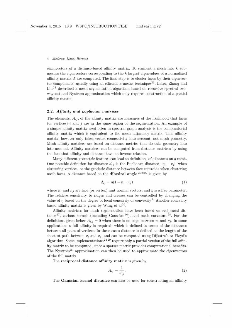
Many different geometric features can lead to definitions of distances on a mesh.
One possible definition for distance dij is the Euclidean distance ||vi − vj || whenclustering vertices, or the geodesic distance between face centroids when clustering
mesh faces. A distance based on the dihedral angle25;4;22 is given by
dij = η(1− ni · nj) (1)
where ni and nj are face (or vertex) unit normal vectors, and η is a free parameter.
The relative sensitivity to ridges and creases can be controlled by changing the
value of η based on the degree of local concavity or convexity4. Another concavity
based affinity matrix is given by Wang et al26.
Affinity matrices for mesh segmentation have been based on reciprocal dis-
tance27, various kernels (including Gaussian10), and mesh curvature28. For the
definitions given below Ai,j = 0 when there is no edge between vi and vj . In some
applications a full affinity is required, which is defined in terms of the distances
between all pairs of vertices. In these cases distance is defined as the length of the
shortest path between vi and vj , and can be computed using Dijkstra’s or Floyd’s
algorithm. Some implementations24 29 require only a partial version of the full affin-
ity matrix to be computed, since a sparser matrix provides computational benefits.
The Nystrom30 approximation can then be used to approximate the eigenvectors
of the full matrix.
The reciprocal distance affinity matrix is given by
Aij =1
dij. (2)
The Gaussian kernel distance can also be used for constructing an affinity

November 4, 2015 10:9 WSPC/INSTRUCTION FILE nmf˙seg˙ijig˙v2
Sparse Non-negative Matrix Factorization for Mesh Segmentation 5
matrix,
Aij = e−d(vi,vj)
2
2σ2 (3)
where σ is a tunable parameter that influences the size of the clusters, and d may
be Euclidean distance or some other measure. Liu and Zhang22 use a function, d
based on face centroid geodesic distance and face dihedral angle. They also suggest
a method for automatically computing σ.
Early graph partitioning9 and image segmentation10 methods were based on the
eigenvectors of the affinity matrix. Later methods operated instead on the Laplacian
matrix, which is computed from the affinity matrix, but can be defined in many
ways. The study of eigenvalues of the Laplacian matrix has connections to harmonic
analysis where basis functions on various domains (e.g. DCT, Fourier basis, spher-
ical harmonics) can be formulated as eigenfunctions of Laplacian operators defined
on those domains. Other mesh segmentation techniques based on this eigenfunction
concept include5;31;25;32. Methods based on eigenfunctions of the Laplace-Beltrami
operator include diffusion distance and heat kernel signature18.
Most Laplacian formulations are defined in terms of the diagonal matrix D,
where Dii =∑
j Aij . In the case of the combinatorial affinity matrix D repre-
sents the degree of each vertex. Variations on spectral clustering can be created by
changing the definition of the affinity matrix and mesh Laplacian.
The symmetric Laplacian, (or graph Laplacian)
L = D −A (4)
was used for mesh segmentation by Liu and Zhang28 and for mesh segmentation
by Zhang et al.25. The normalized Laplacian is given by
L = I −D−1A, (5)
where I is the identity matrix and D−1A is the (row) normalized affinity matrix.
If the eigenvalues of a normalized affinity matrix are λi then the eigenvalues
of the corresponding Laplacian matrix are 1 − λi and the eigenvectors are the
same. The clustering information is contained in the eigenvectors corresponding
to the largest eigenvalues of the affinity matrix, or the smallest eigenvalues of
the Laplacian matrix. Since some popular iterative eigenvalue solvers (e.g. Arnoldi
Iteration) produce the largest magnitude eigenvalues first it can be more efficient
to work in terms of the affinity matrix. Von Luxburg33 gives a thorough overview
of Laplacian matrices used in spectral mesh clustering, and their properties.
Once the desired matrix, M , (affinity matrix, normalized affinity matrix or
Laplacian matrix) is computed, the next step of spectral segmentation is to compute
the eigenvalue decomposition M = XΛX−1 where Λ is a diagonal matrix. The
eigenvectors xi are the columns of X, and the eigenvalues λi = Λii are assumed to
sorted. Segmentation into k regions requires the k eigenvectors which correspond
to the k smallest or largest eigenvalues. The eigenvectors are assembled into U =
[x1, x2, ..., xk]. Finally k-means clustering on the rows of U is performed to find

November 4, 2015 10:9 WSPC/INSTRUCTION FILE nmf˙seg˙ijig˙v2
6 McGraw, Kang, Herring
the segmentation result. It is also possible to automatically estimate the number of
regions from Λ by using the eigengap heuristic maxk = λk+1 − λk. An overview of
spectral mesh segmentation is given in Algorithm (1).
Like spectral methods, our segmentation algorithm also requires computation of
an affinity matrix. In place of the eigenvalue decomposition we compute the sparse
rank-k NMF. Since the Laplacian matrix can have negative values it cannot be
decomposed by the NMF. Instead we compute the NMF of a normalized affinity
matrix, M = D−1A. The segmentation results are directly extracted from the
NMF, M = WH, by finding the column of H which has maximum value. Due to
the clustering properties of NMF we don’t need to perform any additional clustering
on the results.
Algorithm 1 Spectral mesh segmentation
1: procedure Spectral mesh segmentation(V, F, k)
2: Compute the dual graph V ′, F ′. Use the dual graph in the following computa-
tions where vertices correspond to faces of the original mesh.
3: Compute the distance matrix d
4: Estimate σ for the Gaussian kernel affinity matrix.
5: Compute an affinity matrix, A from the distance matrix, d and σ.
6: Compute the full affinity matrix for all vertex pairs (e.g. using Floyd-Warshall
or Dijkstra)
7: From A compute a normalized affinity matrix.
8: Compute the eigenvalue decomposition S = V ΛV −1 and sort the eigenvalues
(diagonal elements of Λ) and the corresponding eigenvectors.
9: Extract the last k columns of V into V .
10: Normalize the rows of V , as done by20.
11: Compute k-means on the rows of V . The clustering assignment of each vertex
gives segmentation results
12: end procedure
Decomposition of a normalized affinity matrix has previously been used to per-
form clustering in the context of stochastic processes. Meila and Shi34 perform
clustering by analyzing the row normalized matrix M = D−1A. This matrix can be
interpreted as a stochastic matrix where Mij is the probability of a random walk
moving from vertex i to j in one step. Eigenanalysis of this matrix can reveal the
regions that random walks remain in for large amounts of time.
3. Sparse non-negative matrix factorization
Non-negative matrix factorization is used by many unsupervised learning algo-
rithms that yield a parts-based representation of data. The non-negativity of the
resulting matrices means that the data can be expressed as a strictly additive com-

November 4, 2015 10:9 WSPC/INSTRUCTION FILE nmf˙seg˙ijig˙v2
Sparse Non-negative Matrix Factorization for Mesh Segmentation 7
Fig. 1. Local basis functions computed from 1500 face images (left), sample 19× 19 face image
bination of parts. As a result, NMF usually results in an intuitive decomposition
of the data since additional terms cannot subtract already existing features in the
data. For example, NMF is an integral part of algorithms for blind source separa-
tion of audio signals, such as music. A musical score may be decomposed into the
individual instrument tracks35. NMF analysis of stochastic matrices can be used to
learn statistical models of random processes13.
The problem of finding the NMF can be written as the optimization problem
minW,H
||L−WH||2F s.t. W ≥ 0 and H ≥ 0 (6)
where || · ||F denotes the matrix Frobenius norm.
3.1. Parts-based decomposition and clustering with NMF
To demonstrate NMF with a sample image processing application, we replicated
the experiments of Lee and Seung15 by applying NMF to a facial image database36
of 1500 images. Each 19× 19 pixel image was reformatted to 1D, and was set as a
column of L. The NMF (rank = 49) of L was computed, and the facial features were
extracted from the columns of W . Computing the NMF of the 361 × 1500 matrix
took 0.25 seconds in Matlab. Unlike the eigenface approach, where the eigenvalue
decomposition of a covariance matrix is computed, the NMF features are local.
The 49 features shown in Figure (1) often correspond to recognizable features such
as eyes, nose and lips. Since the coefficient matrix is positive, the features can be
added together in an intuitive way to form the image of face.
The fact that symmetric NMF can be shown to be equivalent to kernel k-means
clustering37 suggests the usefulness of NMF as a segmentation tool. The equiva-
lence can be seen by using the fact that the kernel k-means objective function can
be written in terms of matrix trace maximization38. The trace maximization prob-
lem maxH tr(HTLH) can be shown to be equivalent to the minimization problem
minH ||L−HHT || which defines the symmetric NMF problem L = HHT .

November 4, 2015 10:9 WSPC/INSTRUCTION FILE nmf˙seg˙ijig˙v2
8 McGraw, Kang, Herring
3.2. Sparsity
Many recently developed solutions to image processing problems are formulated
by transforming the problem into a domain in which the data are sparse. Sparsity
means that a signal can expressed as linear combination of basis functions using few
terms. This has obvious implications for data compression39. Other image analysis
applications are image reconstruction40, and denoising41. Though the NMF often
results in sparse basis functions, by imposing a sparseness constraint the degree of
sparseness can be controlled42.
Sparseness can be quantified using the l0 norm which counts the number of
nonzero elements in a vector. Equation (7) shows the constrained optimization
problem that solves the linear system x = Dy while imposing sparseness on the
solution y.
miny
1
2||x−Dy||22 + λ||y||0 (7)
However, solution of Equation 7 is NP-hard. In many cases43 the convex re-
laxation of Equation 7 formed by replacing the l0 norm with the l1 norm induces
sparsity in y and can be solved much more efficiently.
Imposing a sparseness constraint on either, or both of the the factors W and H
has several benefits. In general the NMF does not have a unique solution, but by
imposing some constraints it can be made unique. Sparsity, unfortunately, is not one
of those constraints. But the computation of the sparse NMF does have a smaller
solution space and has been shown to lead to better and more consistent clustering
results44. Increasing sparsity has also been observed to improve the separation of
features35 in the resulting basis vectors.
Incorporating sparseness on H into the NMF decomposition results in the op-
timization problem
minW,H
1
2||L−WH||2F +
µ
2||W ||2F +
λ
2
∑
i
||hi||21 s.t. W ≥ 0 and H ≥ 0
where hi are columns of H. The Frobenius norm term controlled by parameter µ
adds another side constraint that keeps W from becoming too large which would
in turn cause H to become very small.
The sparse NMF problem can be solved by initializing H to non-negative ran-
dom values, then solving alternating non-negative least squares (NNLS) problems.
When solving for H by NNLS, W is held constant
minH>0
∣
∣
∣
∣
∣
∣
∣
∣
(
W√λe1×k
)
H −(
L
01×n
)∣
∣
∣
∣
∣
∣
∣
∣
2
F
, (8)
where e1×k is a row of zeros, and 01×n is a column of all zeros. Likewise, H is held
constant when solving for W by
minW>0
∣
∣
∣
∣
∣
∣
∣
∣
(
HT
õIk
)
WT −(
L
0k×m
)∣
∣
∣
∣
∣
∣
∣
∣
2
F
, (9)

November 4, 2015 10:9 WSPC/INSTRUCTION FILE nmf˙seg˙ijig˙v2
Sparse Non-negative Matrix Factorization for Mesh Segmentation 9
where Ik is a k × k identity matrix, and 0k×m is a k × m matrix of all zeroes.
Alternation continues until an iteration threshold has been passed or the fitting
residual falls below some threshold. See Li and Ngom45 for a full description of this
and other NMF decomposition algorithms and source code.
4. Methods
Algorithm 2 NMF segmentation
1: procedure NMF mesh segmentation(V, F, n, k)
2: Compute the dual graph of the mesh to obtain V ′, F ′.
3: Compute the same distance matrix, d, as Katz4 and Liu and Zhang22 which is
based on a combination of geodesic distance and dihedral angle (Equation (1)).
4: Compute the distance-based affinity matrix, A, from d using Equation(2).
5: From A, compute T , the all pairs shortest path matrix22.
6: Compute S = D−1T , the normalized affinity matrix, by normalizing the rows
of T to sum to 1. S can be seen as a Markov transition matrix describing a
random walk on the mesh. Each element, Ti,j , represents the probability of a
random walk going from face i to face j.
7: Compute the rank-k sparse NMF of S to obtain W and H, where k is the
number of desired regions.
8: Normalize W and H.
9: Compute the label for each face, i by finding maxjHi,j
10: end procedure
We solve the mesh segmentation problem using the steps described in Algo-
rithm (2). In comparing this implementation to other clustering and segmentation
approaches, note that
• We have found that the same parameter ranges used by Liu and Zhang22
in computing distances (δ ∈ [0.01, 0.05] and η ∈ [0.1, 0.2]) perform well, so
we use the same range.
• We decompose an asymmetric normalized affinity matrix rather than a
symmetric normalized affinity or Laplacian matrix.
• We don’t need to estimate a variance for the kernel-based affinity (Equation
3).
• We don’t compute eigenvalues, so we don’t need to sort eigenvalues or row
normalize eigenvectors
• We don’t need a separate k-means clustering step since the nature of NMF
produces clusters in the matrix of basis functions, H.
To demonstrate the parts based decomposition found by the NMF we show
the basis functions H:,j for several meshes in Figures (2, 4, and 5). The rank, k,

November 4, 2015 10:9 WSPC/INSTRUCTION FILE nmf˙seg˙ijig˙v2
10 McGraw, Kang, Herring
of the decomposition is set to the number of desired regions. Note that the basis
functions computed for the head mesh, like the image decomposition results in
Figure (1), highlight local anatomical features like the eyes, ears and nose. This is
not the case for other basis functions, such as the diffusion wavelet basis46 or the
eigenfunctions of the Laplace-Beltrami operator shown in Figure (3). The superior
locality of the NMF basis is due to several factors: (1) the affinity matrix takes
geodesic distance between faces into account resulting in surface clustering, (2) the
NMF generates an additive decomposition of the mesh into local parts, and (3) the
sparseness constraint drives low values in the NMF basis functions to zero, resulting
in a sharper delineation of features.
Fig. 2. NMF basis functions (k = 12) for the head mesh plotted with a heat map color palette.
White denotes high values, and black denotes low values. Features such as eyes, ears and nose areclearly visible.
Fig. 3. Other comparable basis functions. Diffusion wavelet basis functions (top) and eigenfunctionsof the Laplace-Beltrami operator (bottom) are not a local nor as feature specific as the NMF basis
functions.
For segmentation, sparsity is enforced on the columns of H, which is the clus-
ter indicator function. Sparsity on H encourages locality of the clusters. Figure 6

November 4, 2015 10:9 WSPC/INSTRUCTION FILE nmf˙seg˙ijig˙v2
Sparse Non-negative Matrix Factorization for Mesh Segmentation 11
Fig. 4. NMF basis functions (k = 5) for the table mesh. The table top and each leg are isolatedin different functions.
Fig. 5. NMF basis functions (k = 6) for the hand mesh. Each finger is strongly associated with adifferent function.
demonstrates the effect of sparsity on theH and the segmentation results. In the top
row the basis functions without sparsity do not reflect a clear distinction between
the three regions in the mesh. In the bottom row the sparse basis functions show a
clear separation of regions which permits us to use a simple columnwise maximum
operation to assign clusters to faces. The segmentation results are clearly improved
with the sparsity constraint as the helmet, face and base are assigned to different
regions.
Fig. 6. Basis functions (left) and segmentation results (right) computed without (top) and with(bottom) sparseness constraints (k = 3).
5. Results
In this section we present our experimental results and demonstrate the perfor-
mance of our algorithm compared to spectral approaches. We tested the NMF
segmentation approach on meshes from the Princeton Shape Benchmark, McGill
3D shape benchmark, and AIM@SHAPE-VISIONAIR repositories. For all results
we have used parameter values δ ∈ [0.01, 0.05], η ∈ [0.1, 0.2], n = 10. The value of
k is noted in the figure captions.

November 4, 2015 10:9 WSPC/INSTRUCTION FILE nmf˙seg˙ijig˙v2
12 McGraw, Kang, Herring
Fig. 7. Segmentation results on flamingo (k=4), dragon (k=6), armadillo (k=6), skeleton (k=7),pawn (k=4), hand (k=6), Lucy (k=10) and happy Buddha (k=6) and meshes.
Figure (7) shows successful results of our method on flamingo, skeleton, pawn
and hand meshes. The flamingo was segmented into four regions which correspond
to the body, two legs and the neck and head together in a single region. The NMF
method combined with the choice of affinity matrix handles narrow extremities
very well due to the inclusion of a dihedral distance term. The skeleton result is
particularly impressive since there are many small bones and concave features that
could have confounded the segmentation process. The pawn doesn’t have any long
protrusions, like the other meshes, but small concave valleys between the parts lead
to a good result.
One case in which our method performed better than spectral segmentation is
the octopus mesh shown in Figure 8. Note that our method has placed all of the
Fig. 8. Segmentation results on octopus (k=9) using our method (left) and spectral mesh segmen-
tation (right).
legs of the octopus into different regions while spectral segmentation produced a
segmentation where two legs were in the same region (colored cyan), and a separate
region appears near the base of the yellow leg.
Successful segmentations of animals in anatomical regions are shown in

November 4, 2015 10:9 WSPC/INSTRUCTION FILE nmf˙seg˙ijig˙v2
Sparse Non-negative Matrix Factorization for Mesh Segmentation 13
Figure(9). On the horse and camel we are able to split the animals into leg, head
and body regions. On the bunny mesh the head, ears, feet and tail are separate
from the chest, back and thigh.
Fig. 9. Animal segmentation results. Camel (k=6), horse (k=6) and bunny (k=8).
Figure 10 shows a mesh for which NMF did not produce a good result. A
semantic segmentation would have a region representing the hub at the center of
the rocker arm and regions for the adjusting screw and nut at the top. Our method
was able to segment the screw and nut, but not the hub. Spectral segmentation did
a better job, but not ideal. That method was able to segment the hub and one end
of the screw. These results are probably due to the relative flatness and smoothness
of the mesh. Both methods would likely perform better by changing the affinity
matrix to weight angular distance more or take some other geometric features into
account.
Fig. 10. Segmentation of rocker arm (k=4) with NMF method (left) and spectral method (right).Both methods fail to produce a meaningful result.
Meshes that consist of multiple connected components (such as the handle,
spout, lid and body of the teapot) and non-watertight meshes such as the teapot can
be segmented. The hand mesh shown on the right side of Figure (11) demonstrates
that NMF mesh segmentation can produce meaningful results in the presence of
additive noise. In this experiment the input mesh had its vertices displaced in
the normal direction by a random distance (zero-mean Gaussian with standard
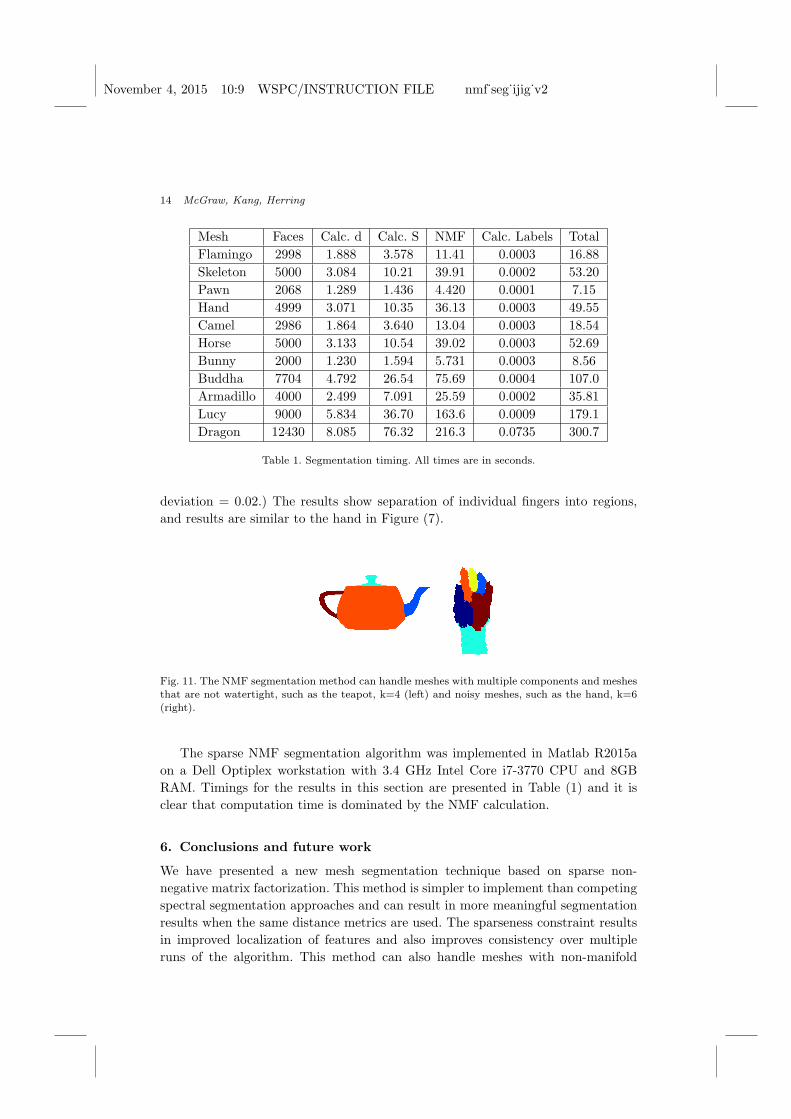
November 4, 2015 10:9 WSPC/INSTRUCTION FILE nmf˙seg˙ijig˙v2
14 McGraw, Kang, Herring
Mesh Faces Calc. d Calc. S NMF Calc. Labels Total
Flamingo 2998 1.888 3.578 11.41 0.0003 16.88
Skeleton 5000 3.084 10.21 39.91 0.0002 53.20
Pawn 2068 1.289 1.436 4.420 0.0001 7.15
Hand 4999 3.071 10.35 36.13 0.0003 49.55
Camel 2986 1.864 3.640 13.04 0.0003 18.54
Horse 5000 3.133 10.54 39.02 0.0003 52.69
Bunny 2000 1.230 1.594 5.731 0.0003 8.56
Buddha 7704 4.792 26.54 75.69 0.0004 107.0
Armadillo 4000 2.499 7.091 25.59 0.0002 35.81
Lucy 9000 5.834 36.70 163.6 0.0009 179.1
Dragon 12430 8.085 76.32 216.3 0.0735 300.7
Table 1. Segmentation timing. All times are in seconds.
deviation = 0.02.) The results show separation of individual fingers into regions,
and results are similar to the hand in Figure (7).
Fig. 11. The NMF segmentation method can handle meshes with multiple components and meshesthat are not watertight, such as the teapot, k=4 (left) and noisy meshes, such as the hand, k=6(right).
The sparse NMF segmentation algorithm was implemented in Matlab R2015a
on a Dell Optiplex workstation with 3.4 GHz Intel Core i7-3770 CPU and 8GB
RAM. Timings for the results in this section are presented in Table (1) and it is
clear that computation time is dominated by the NMF calculation.
6. Conclusions and future work
We have presented a new mesh segmentation technique based on sparse non-
negative matrix factorization. This method is simpler to implement than competing
spectral segmentation approaches and can result in more meaningful segmentation
results when the same distance metrics are used. The sparseness constraint results
in improved localization of features and also improves consistency over multiple
runs of the algorithm. This method can also handle meshes with non-manifold

November 4, 2015 10:9 WSPC/INSTRUCTION FILE nmf˙seg˙ijig˙v2
REFERENCES 15
edges that are not watertight and consist of multiple connected components.
6.1. Limitations
Mesh size and region count are limited by system memory. We have run out of
memory on a 64-bit system with 8GB of RAM while segmenting a mesh with 50000
faces. This is because the matrix, S, assembled in algorithm 2 is a full matrix with
size |F | × |F | where |F | is the number of faces in the mesh. Likewise, spectral
mesh clustering22, requires construction of a dense pairwise face distance matrix.
But the memory requirements of our implementation of the NMF are greater than
the eigenvalue decomposition. We are investigating patch-based and multiresolution
approaches to segmenting large meshes and more memory efficient implementations
of NMF.
We have observed that NMF segmentation results depend on triangle quality.
The same is noted for spectral segmentation. Using an area weighting when com-
puting the affinity matrix, as is done in the conformal Laplacian, may help reduce
the impact of triangle quality.
Sometimes computing segmentation labels with the max operation results in
disconnected regions having the same label. This can be fixed by splitting discon-
nected regions into multiple labels, resulting in a segmentation with more than k
regions.
6.2. Improvements
There are several areas of improvement to the proposed algorithm. The row maxi-
mum operation for assigning clusters to faces is a simple and obvious approach, but
replacing it with a more sophisticated process may improve the quality of clusters
and result in smoother boundaries. Another approach to smoothing the segmenta-
tion boundaries may be to directly filter the basis functions. To compare our results
with spectral mesh clustering22 we used the same distance matrix, but more exper-
iments are needed to see if the NMF approach can be improved by using a different
distance metric.
6.3. Applications
The parts-based local basis functions computed by the sparse NMF may be useful
for other applications, such as automatically computed bone weights for skeletal
animation. We will also explore the use of these basis functions for feature detection
in applications such as shape matching and mesh retrieval.
Bibliography
References
1. J. Shotton, T. Sharp, A. Kipman, A. Fitzgibbon, M. Finocchio, A. Blake,
M. Cook, and R. Moore, “Real-time human pose recognition in parts from sin-

November 4, 2015 10:9 WSPC/INSTRUCTION FILE nmf˙seg˙ijig˙v2
16 REFERENCES
gle depth images,” Communications of the ACM, vol. 56, no. 1, pp. 116–124,
2013.
2. A. Sheffer, E. Praun, and K. Rose, “Mesh parameterization methods and
their applications,” Foundations and Trends in Computer Graphics and Vi-
sion, vol. 2, no. 2, pp. 105–171, 2006.
3. X. Li, T. W. Woon, T. S. Tan, and Z. Huang, “Decomposing polygon meshes for
interactive applications,” in Proceedings of the 2001 symposium on Interactive
3D graphics, pp. 35–42, ACM, 2001.
4. S. Katz and A. Tal, Hierarchical mesh decomposition using fuzzy clustering and
cuts, vol. 22. ACM, 2003.
5. F. De Goes, S. Goldenstein, and L. Velho, “A hierarchical segmentation of
articulated bodies,” in Computer Graphics Forum, vol. 27, pp. 1349–1356, 2008.
6. S. Biasotti, S. Marini, M. Mortara, G. Patane, M. Spagnuolo, and B. Falcidieno,
“3d shape matching through topological structures,” in Discrete Geometry for
Computer Imagery, pp. 194–203, Springer, 2003.
7. T. Funkhouser, M. Kazhdan, P. Shilane, P. Min, W. Kiefer, A. Tal,
S. Rusinkiewicz, and D. Dobkin, “Modeling by example,” in ACM Transac-
tions on Graphics (TOG), vol. 23, pp. 652–663, ACM, 2004.
8. S. Shlafman, A. Tal, and S. Katz, “Metamorphosis of polyhedral surfaces using
decomposition,” in Computer Graphics Forum, vol. 21, pp. 219–228, 2002.
9. W. E. Donath and A. J. Hoffman, “Lower bounds for the partitioning of
graphs,” IBM Journal of Research and Development, vol. 17, no. 5, pp. 420–425,
1973.
10. Y. Weiss, “Segmentation using eigenvectors: a unifying view,” in IEEE Inter-
national Conference on Computer Vision, vol. 2, pp. 975–982, IEEE, 1999.
11. W. Xu, X. Liu, and Y. Gong, “Document clustering based on non-negative ma-
trix factorization,” in Proceedings of the 26th annual international ACM SIGIR
conference on Research and development in informaion retrieval, pp. 267–273,
ACM, 2003.
12. Z. Li, J. Liu, and H. Lu, “Structure preserving non-negative matrix factoriza-
tion for dimensionality reduction,” Computer Vision and Image Understanding,
vol. 117, no. 9, pp. 1175–1189, 2013.
13. G. Cybenko and V. Crespi, “Learning hidden Markov models using nonnega-
tive matrix factorization,” Information Theory, IEEE Transactions on, vol. 57,
no. 6, pp. 3963–3970, 2011.
14. Y. Xie, J. Ho, and B. C. Vemuri, “Nonnegative factorization of diffusion tensor
images and its applications,” in Information Processing in Medical Imaging,
pp. 550–561, Springer, 2011.
15. D. D. Lee and H. S. Seung, “Learning the parts of objects by non-negative
matrix factorization,” Nature, vol. 401, no. 6755, pp. 788–791, 1999.
16. O. D. Faugeras and M. Hebert, “The representation, recognition, and locating
of 3-d objects,” The International Journal of Robotics Research, vol. 5, no. 3,
pp. 27–52, 1986.

November 4, 2015 10:9 WSPC/INSTRUCTION FILE nmf˙seg˙ijig˙v2
REFERENCES 17
17. A. Shamir, “A survey on mesh segmentation techniques,” in Computer Graphics
Forum, vol. 27, pp. 1539–1556, 2008.
18. P. Theologou, I. Pratikakis, and T. Theoharis, “A comprehensive overview of
methodologies and performance evaluation frameworks in 3d mesh segmenta-
tion,” Computer Vision and Image Understanding, 2015.
19. H. Zhang, O. Van Kaick, and R. Dyer, “Spectral mesh processing,” in Computer
Graphics Forum, vol. 29, pp. 1865–1894, 2010.
20. A. Y. Ng, M. I. Jordan, Y. Weiss, et al., “On spectral clustering: Analysis
and an algorithm,” Advances in Neural Information Processing Systems, vol. 2,
pp. 849–856, 2002.
21. B. Vallet and B. Levy, “Spectral geometry processing with manifold harmon-
ics,” in Computer Graphics Forum, vol. 27, pp. 251–260, 2008.
22. R. Liu and H. Zhang, “Segmentation of 3d meshes through spectral clustering,”
in Computer Graphics and Applications, 2004. PG 2004. Proceedings. 12th Pa-
cific Conference on, pp. 298–305, IEEE, 2004.
23. J. A. Hartigan and M. A. Wong, “Algorithm as 136: A k-means clustering
algorithm,” Applied statistics, pp. 100–108, 1979.
24. H. Zhang and R. Liu, “Mesh segmentation via recursive and visually salient
spectral cuts,” in Proc. of vision, modeling, and visualization, pp. 429–436,
2005.
25. J. Zhang, J. Zheng, C. Wu, and J. Cai, “Variational mesh decomposition,”
ACM Transactions on Graphics (TOG), vol. 31, no. 3, p. 21, 2012.
26. H. Wang, T. Lu, O. K.-C. Au, and C.-L. Tai, “Spectral 3d mesh segmentation
with a novel single segmentation field,”Graphical Models, vol. 76, no. 5, pp. 440–
456, 2014.
27. K. C. Das, “Maximum eigenvalue of the reciprocal distance matrix,” J Math
Chem, vol. 47, pp. 21–28, 2010.
28. R. Liu and H. Zhang, “Mesh segmentation via spectral embedding and contour
analysis,” in Computer Graphics Forum, vol. 26, pp. 385–394, 2007.
29. C. Fowlkes, S. Belongie, F. Chung, and J. Malik, “Spectral grouping using the
nystrom method,” Pattern Analysis and Machine Intelligence, IEEE Transac-
tions on, vol. 26, no. 2, pp. 214–225, 2004.
30. E. J. Nystrom, “Uber die praktische auflosung von integralgleichungen mit an-
wendungen auf randwertaufgaben,” Acta Mathematica, vol. 54, no. 1, pp. 185–
204, 1930.
31. Y. Fang, M. Sun, M. Kim, and K. Ramani, “Heat-mapping: A robust approach
toward perceptually consistent mesh segmentation,” in Computer Vision and
Pattern Recognition (CVPR), 2011 IEEE Conference on, pp. 2145–2152, IEEE,
2011.
32. M. Reuter, “Hierarchical shape segmentation and registration via topological
features of Laplace-Beltrami eigenfunctions,” International Journal of Com-
puter Vision, vol. 89, no. 2-3, pp. 287–308, 2010.
33. U. Von Luxburg, “A tutorial on spectral clustering,” Statistics and computing,

November 4, 2015 10:9 WSPC/INSTRUCTION FILE nmf˙seg˙ijig˙v2
18 REFERENCES
vol. 17, no. 4, pp. 395–416, 2007.
34. M. Meila and J. Shi, “A random walks view of spectral segmentation,” Inter-
national Workshop on AI and Statistics, 2001.
35. T. Virtanen, “Monaural sound source separation by nonnegative matrix fac-
torization with temporal continuity and sparseness criteria,” Audio, Speech,
and Language Processing, IEEE Transactions on, vol. 15, no. 3, pp. 1066–1074,
2007.
36. K.-K. Sung, Learning and Example Selection for Object and Pattern Recog-
nition. PhD thesis, MIT, Artificial Intelligence Laboratory and Center for
Biological and Computational Learning, Cambridge, MA, 1996.
37. C. H. Ding, X. He, and H. D. Simon, “On the equivalence of nonnegative matrix
factorization and spectral clustering.,” in SDM, vol. 5, pp. 606–610, SIAM, 2005.
38. I. S. Dhillon, Y. Guan, and B. Kulis, “Kernel k-means: spectral clustering
and normalized cuts,” in Proceedings of the tenth ACM SIGKDD international
conference on Knowledge discovery and data mining, pp. 551–556, ACM, 2004.
39. S. G. Chang, B. Yu, and M. Vetterli, “Adaptive wavelet thresholding for image
denoising and compression,” Image Processing, IEEE Transactions on, vol. 9,
no. 9, pp. 1532–1546, 2000.
40. M. Lustig, D. Donoho, and J. M. Pauly, “Sparse MRI: The application of
compressed sensing for rapid MR imaging,” Magnetic resonance in medicine,
vol. 58, no. 6, pp. 1182–1195, 2007.
41. M. Elad and M. Aharon, “Image denoising via sparse and redundant represen-
tations over learned dictionaries,” Image Processing, IEEE Transactions on,
vol. 15, no. 12, pp. 3736–3745, 2006.
42. P. O. Hoyer, “Non-negative matrix factorization with sparseness constraints,”
The Journal of Machine Learning Research, vol. 5, pp. 1457–1469, 2004.
43. D. L. Donoho, “For most large underdetermined systems of linear equations
the minimal 1-norm solution is also the sparsest solution,” Communications on
pure and applied mathematics, vol. 59, no. 6, pp. 797–829, 2006.
44. J. Kim and H. Park, “Sparse nonnegative matrix factorization for clustering,”
Technical Report, 2008.
45. Y. Li and A. Ngom, “The non-negative matrix factorization toolbox for biolog-
ical data mining,” Source code for biology and medicine, vol. 8, no. 1, pp. 1–15,
2013.
46. R. R. Coifman and M. Maggioni, “Diffusion wavelets,” Applied and Computa-
tional Harmonic Analysis, vol. 21, no. 1, pp. 53–94, 2006.

November 4, 2015 10:9 WSPC/INSTRUCTION FILE nmf˙seg˙ijig˙v2
REFERENCES 19
Photo and Biography
Tim McGraw received the Ph.D. degree in Computer and In-
formation Science and Engineering from University of Florida,
Gainesville, Florida, in 2005.
He has been an Assistant Professor of Computer Graphics
Technology at Purdue University since 2013. His research in-
terests are medical image analysis, scientific visualization and
real-time graphics.
Jisun Kang is an MS student of Computer Graphics Tech-
nology at Purdue University. Her research interests are medical
image processing and visualization.
Donald Herring is an MS student of Computer Graphics Tech-
nology at Purdue University. His research interests are real-time
graphics, game development and non-photorealistic rendering.
Copyright © 2022 FDOKUMEN