Designing Structured Sparse Dictionaries for

Sparse Representation Modeling

G. Tessitore, R. Prevete

Department of Physical Sciences, University of Naples Federico II, Naples, Italyprevete@na.infn.it, tessitore@na.infn.it

Summary. Linear approaches to the problem of unsupervised data dimensionalityreduction consist in finding a suitable set of factors, which is usually called dictio-

nary, on the basis of which data can be represented as a linear combination of thedictionary elements. In recent years there have been relevant efforts for searchingdata representation which are based on sparse dictionary elements or a sparse lin-ear combination of the dictionary elements. Here we investigate the possibility tocombine the advantages of both sparse dictionary elements and sparse linear combi-nation. Notably, we also impose a structure on the dictionary elements. We compareour algorithm with two other different approaches presented in literature whichimpose either sparse structured dictionary elements or sparse linear combination.These (preliminary) results suggests that our approach presents some promising ad-vantages, in particular a greater possibility of interpreting the data representation.

1 Introduction

Unsupervised dimensionality reduction seems to bring relevant benefits inmany contexts which include classification, regression and control problems[12, 13]. Among linear techniques for dimensional reduction Principal Com-ponent Analysis (PCA) [7] is widely used. The PCA approach enables oneto approximate signals as a linear combination of a restricted number of or-thogonal factors that most efficiently explain the data variance. Accordinglya signal composed of a large number of variables can be represented as a smallnumber of coefficients of the linear combination of the factors. The orthogo-nal factors typically involve all original variables. This aspect can cause somedifficulties, notably for the interpretation of the signals expressed as linearcombination of the orthogonal factors. For example, in the context of the re-search on human actions [12] can be useful to determine which “pieces” of theaction are more relevant than others in classifying or controlling the actionitself. In recent years, there has been a growing interest for identifying alter-natives to PCA which find interpretable and more powerful representationsof the signals. In these approaches the factors or the coefficients of the linear

2 G. Tessitore, R. Prevete

combination are obtained using prior information represented by penalizationterms or constraints in a minimization problem. One can isolate two differenttypes of approaches: a) Sparse factors. In this case each factor involves justa small number of the original variables (for example see Sparse-PCA [14]and Structured-Sparse-PCA [9]). b) Sparse linear combination of the factors.Here an overcomplete set of factors is chosen in advance or learned from thedata, but the approximation of each signal involves only a restricted numberof factors. Hence, the signals are represented by sparse linear combinations ofthe factors (for example see K-SVD [1] and MOD [6]). In both approaches, theorthogonality constraint on the factors is usually violated, the set of factorsis called dictionary, and each factor is called dictionary element or atom.

Here we investigate the possibility of combining the advantages of bothapproaches simultaneously finding sparse dictionary elements and sparse lin-ear combination of the dictionary elements. Importantly, in addition to sparsedictionary elements we also impose a structure on the atoms [9]. To this aim,we propose a method for Sparse Representation with Structured Sparse Dic-tionary (SR-SSD). Our approach is tested by using both synthetic and realdatasets. The rest of the paper is organized as follows: In Section 2, we givethe theoretical formulation of the problem. The description of our algorithmand its relation to previously proposed method is presented in Section 3. Theresults of our algorithm on synthetic and real data, compared with the re-sults of other two standard algorithms, are presented in Section 4. Finally, inSection 5 we discuss the results obtained and draw our main conclusions.

Notations: Bold uppercase letters refer to matrices, e.g., X,V, and boldlowercase letters designate vectors, e.g., x,v. We denote by Xi and Xj the i-throw and the j-th column of a matrix X, respectively. While we use the notationxi and vij to refer to the i-th element of the vector x and the element in thei-th row and the j-th column of the matrix V, respectively. Given x ∈ R

p

and q ∈ [1,∞), we use the notation ‖x‖q to refer to its lq-norm definedas ‖x‖q = (

∑pi=1 |xi|

q)1/q. Given two vectors x and y in Rp, we denote by

x y = (x1y1, x2y2, ..., xpyp)T ∈ Rp the element-wise product of x and y.

2 Problem statement

Let us define a matrix X ∈ Rn×p of n rows in R

p, each one correspondingto an experimental observation, the learning problem we are addressing canbe solved by finding a matrix V ∈ R

p×r such that each row of X can beapproximated by a linear combination of the r columns of V. V is the dictio-nary, and the r columns Vk of V are the dictionary elements or atoms. Letus call U ∈ R

n×r the matrix of the linear combination coefficients, i.e., thei-th row of U corresponds to the r coefficients of the linear combination ofthe r columns of V in order to approximate the i-th row of X. Consequently,UVT is an approximation of X. The learning problem can be expressed as:

Structured Sparse Dictionaries for Sparse Representation 3

minU,V

1

2np‖X−UVT ‖2F + λ

r∑

k=1

Ωv(Vk) s.t. ∀j,Ωu(Uj) < T0 (1)

where Ωv(Vk) and Ωu(Uj) are some norms or quasi-norms that constrain

or regularize the solutions of the minimization problem, and λ ≥ 0 and T0 >

0 are parameters that controls to which extension the dictionary and thecoefficients are regularized. If one assumes that both regularizations Ωu andΩv are convex, for V fixed the problem (1) is convex w.r.t. U and vice versa.

As we want to induce a sparsity for the linear combination of the dictionaryelements, we can choose either ℓ0 or ℓ1 norm for the coefficients. These normspenalize linear combinations containing many coefficients different from zero.If not specified differently, we make the following choice: Ωu(Uh) = ‖Uh‖0.

Following [9] the structured sparsity of the dictionary elements can beimposed by choosing

Ωv(Vk) =

s∑

i=1

‖ di Vk ‖α2

1

α

(2)

where α ∈ (0, 1), and each di is a p-dimensional vector satisfying thecondition dij ≥ 0, with i = 1, 2, ..., s. The s vectors di allow to define the

structure of the dictionary elements. More specifically each di individuates agroup of variables corresponding to the set Gi =

j ∈ 1, . . . , p : dij = 0

.

The norm ‖ di Vk ‖α2 penalizes the variables for which dij > 0 and therefore

induces non zero values for variables vjk with j ∈ Gi. The resulting set ofselected variables depends on the contribution of each di as described in [8].For example, if the vectors di induce a partition on the set 1, . . . , p, thenthe penalization term (2) favours the formation of dictionary elements Vk

composed of non-zero variables belonging to just one part of the partition.From [9], who in turn follows [10], the problem (1) considering (2) can bereformulated as follows:

minU,V,H

1

2np‖X−UVT ‖2F +

λ

2

r∑

k=1

[

(Vk)TDiag(Zk)−1Vk) + ‖Hk‖β

]

s.t. ∀j,‖Uj‖0 ≤ T0

(3)

where H ∈ Rr×s+ is a matrix satisfying the condition hki ≥ 0, and β = α

2−α .

The matrix Z ∈ Rp×r is defined as zjk =

∑si=1

(

dij)2

(hki)−1

−1

. Notice that

minimizer of 3 for fixed both U and V is given in a closed form, and it is equalto hki = hki = |y

ki |

2−α‖yk‖α−1α , for k = 1, 2, ..., r and i = 1, 2, ..., s, where each

yk ∈ R1×s is the vector yk = (‖d1 Vk‖2, ‖d

2 Vk‖2, . . . , ‖ds Vk‖2).

In order to solve the problem (3), we follow the usual approach of findingthe minimum by alternating optimizations with respect to the values H, tothe coefficients U and to the dictionary V. Most methods are based on thisalternating scheme of optimization [2].

4 G. Tessitore, R. Prevete

3 SR-SSD Algorithm

SR-SSD algorithm proposed here is composed of three alternate stages: Up-date of the matrix H , Sparse Coding Stage, and Structured Dictionary Stage.Notice that the problem 3 is convex in U for fixed V and vice versa.

Update of matrix H. In this stage, we assume that both U and V

are fixed and update the H’s values. As said above, one can update H by astraightforward equation hki = hki = |yki |

2−α‖yk‖α−1α , however in order to

avoid numerical instability near zero a smoothed update is used as follows:Hk ← maxHk, ǫ with ǫ≪ 1.

Sparse Coding Stage . The second stage of the algorithm proposed hereconsists in updating the U’s values in such a way to obtain a sparse repre-sentation of the signals X, for fixed both V and H . Note that the equation(3) is composed of two terms to be minimized, and the second term does notdepend on U. Therefore, the optimization problem posed in (3) can be, in thisstage, reformulated as follows: minU ‖X−UVT ‖2F s.t. ∀j, ‖Uj‖0 ≤ T0. Thereare a number of well-known “pursuit algorithms” which finds an approximatesolution for this type of problem (see for example Basis Pursuit (BP) [4] andOrtoghonal Matching Pursuit (OMP) [11]). In our approach we use OMP inexperiments in Section 4.1 whereas Iterative Soft-Thresholding (IST) algo-rithm [3] for experiments described in Section 4.2 where we replaced the ℓ0with the ℓ1 norm.

Structured Dictionary Element Stage . The update of the dictionaryV is performed in this stage, and, more importantly, following the approachsuggested by [9] a structured sparse representation for the atoms is found.Fixed both U and H the problem (3) can be reformulated as follows

minV

1

2‖X−UVT ‖2F +

λnp

2

r∑

k=1

(Vk)TDiag(Zk)−1Vk) (4)

Although in this case both the two terms of the problem 4 are convex anddifferentiable with respect to V, for fixed both U and H, leading to a closedform solution for each row of V, in order to avoid p matrix inversions, weconsider a proximal method to update V:

Vk ← Diag(Zk)Diag(‖Uk‖22Zk+npλI)−1(XTUk−VUTUk+‖Uk‖22V

k) (5)

where the update rule is obtained by composing a forward gradient descentstep on the first term with the proximity operator of the second term of (4).

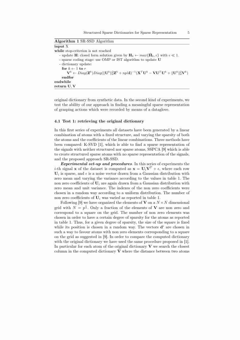
A description of our method is given in Algorithm 1.

4 Experiments

Two different kinds of experiments were conducted: the first series of experi-ments is aimed at testing the ability of the proposed method in retrieving the

Structured Sparse Dictionaries for Sparse Representation 5

Algorithm 1 SR-SSD Algorithm

input Xwhile stop-criterion is not reached

- update H: closed form solution given by Hk ← maxHk, ǫ with ǫ≪ 1.- sparse coding stage: use OMP or IST algorithm to update U

- dictionary update:for k ← 1 to r

Vk ← Diag(Zk)Diag(‖Uk‖22Zk + npλI)−1(XTUk −VUTUk + ‖Uk‖22V

k)endfor

endwhile

return U,V

original dictionary from synthetic data. In the second kind of experiments, wetest the ability of our approach in finding a meaningful sparse representationof grasping actions which were recorded by means of a dataglove.

4.1 Test 1: retrieving the original dictionary

In this first series of experiments all datasets have been generated by a linearcombination of atoms with a fixed structure, and varying the sparsity of boththe atoms and the coefficients of the linear combinations. Three methods havebeen compared: K-SVD [1], which is able to find a sparse representation ofthe signals with neither structured nor sparse atoms, SSPCA [9] which is ableto create structured sparse atoms with no sparse representation of the signals,and the proposed approach SR-SSD.

Experimental set-up and procedures. In this series of experiments thei-th signal x of the dataset is computed as x = UiV

T + ǫ, where each rowUi is sparse, and ǫ is a noise vector drawn from a Gaussian distribution withzero mean and varying the variance according to the values in table 1. Thenon zero coefficients of Ui are again drawn from a Gaussian distribution withzero mean and unit variance. The indexes of the non zero coefficients werechosen in a random way according to a uniform distribution. The number ofnon zero coefficients of Ui was varied as reported in table 1.

Following [9] we have organized the elements of V on a N×N dimensional

grid with N = p1

2 . Only a fraction of the elements of V are non zero andcorrespond to a square on the grid. The number of non zero elements waschosen in order to have a certain degree of sparsity for the atoms as reportedin table 1. Thus, for a given degree of sparsity, the size of the square is fixedwhile its position is chosen in a random way. The vectors d

i are chosen insuch a way to favour atoms with non zero elements corresponding to a squareon the grid as suggested in [9]. In order to compare the computed dictionarywith the original dictionary we have used the same procedure proposed in [1].In particular for each atom of the original dictionary V we search the closestcolumn in the computed dictionary V where the distance between two atoms

6 G. Tessitore, R. Prevete

(r) num. atoms 50(p) dim. signals 400(L) num. atoms for each signals (SR-SSD, K-SVD) 2, 8, 16(ǫ) noise std σ 0, 0.025, 0.05, 0.075, 0.125(n) number of signals 250percentage of zero elements of the atoms 75%, 90%, 99%log2(λ) is searched in the range [−11,−19] at step −1

Table 1. Parameters used for Test 1.

Vj and Vk is defined as 1−|

(

Vj)T

Vk|. A distance less than 0.01 is considered

a success. For both SSPCA and SR-SSD methods the regularization parameterλ has been chosen by a 5-fold cross validation on the representation error. Forall methods the number of atoms to retrieve has been set to the number r ofatoms composing the original dictionary.

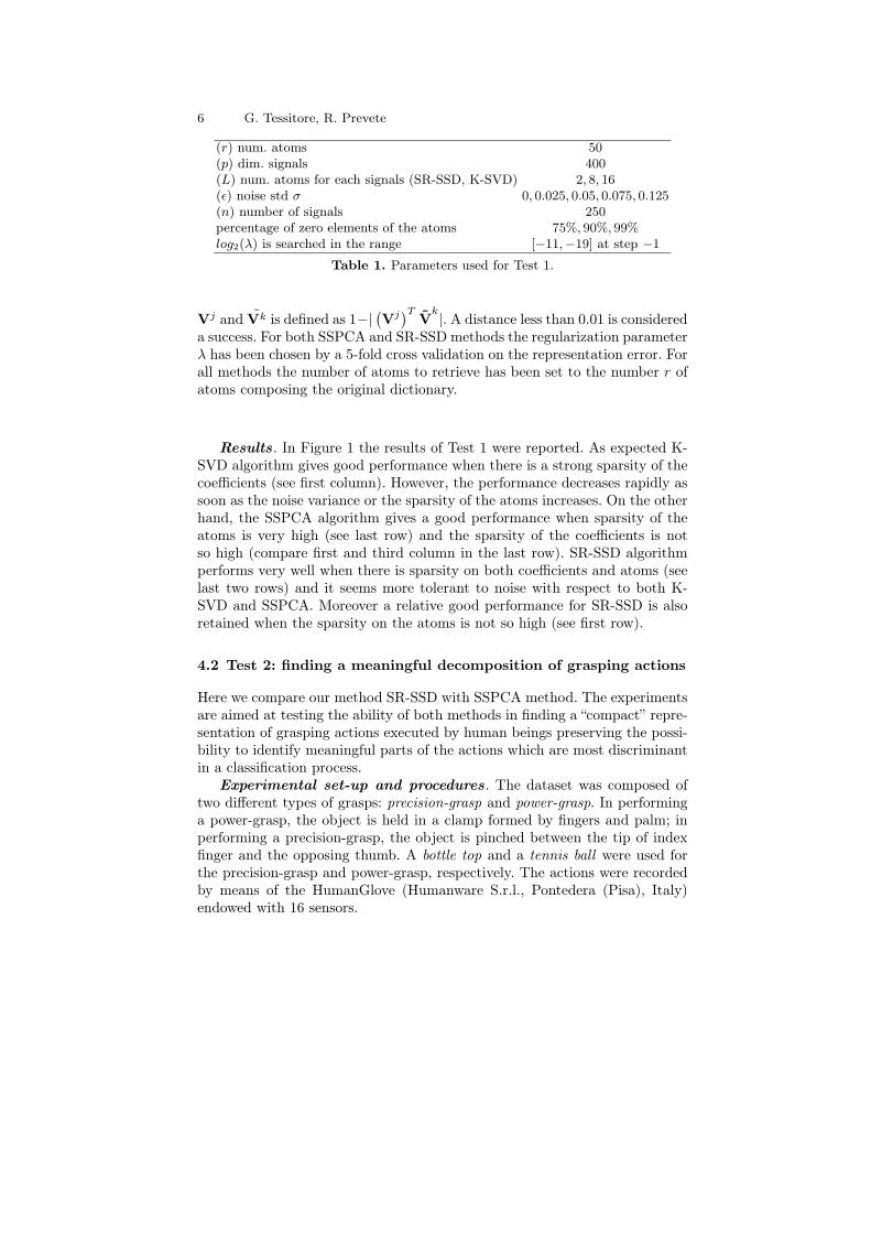
Results. In Figure 1 the results of Test 1 were reported. As expected K-SVD algorithm gives good performance when there is a strong sparsity of thecoefficients (see first column). However, the performance decreases rapidly assoon as the noise variance or the sparsity of the atoms increases. On the otherhand, the SSPCA algorithm gives a good performance when sparsity of theatoms is very high (see last row) and the sparsity of the coefficients is notso high (compare first and third column in the last row). SR-SSD algorithmperforms very well when there is sparsity on both coefficients and atoms (seelast two rows) and it seems more tolerant to noise with respect to both K-SVD and SSPCA. Moreover a relative good performance for SR-SSD is alsoretained when the sparsity on the atoms is not so high (see first row).

4.2 Test 2: finding a meaningful decomposition of grasping actions

Here we compare our method SR-SSD with SSPCA method. The experimentsare aimed at testing the ability of both methods in finding a “compact” repre-sentation of grasping actions executed by human beings preserving the possi-bility to identify meaningful parts of the actions which are most discriminantin a classification process.

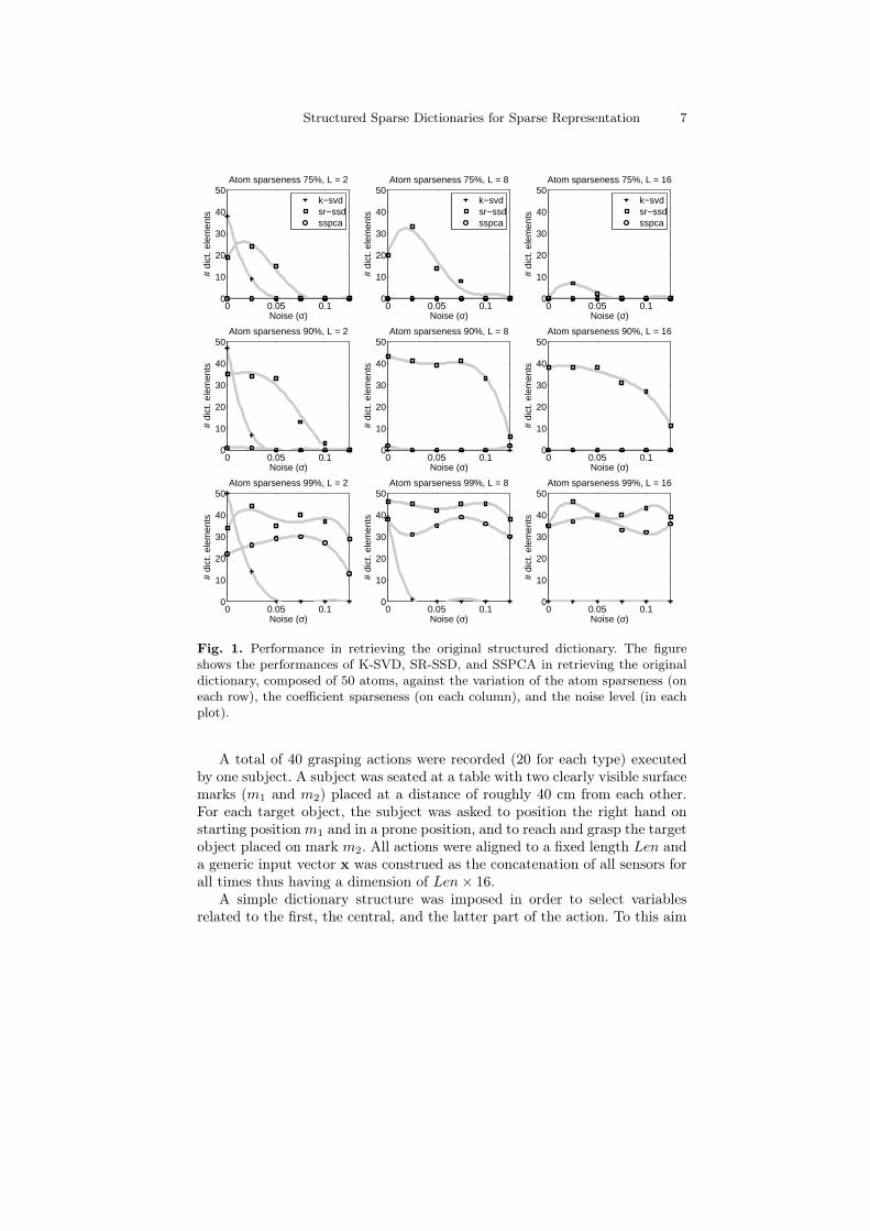
Experimental set-up and procedures. The dataset was composed oftwo different types of grasps: precision-grasp and power-grasp. In performinga power-grasp, the object is held in a clamp formed by fingers and palm; inperforming a precision-grasp, the object is pinched between the tip of indexfinger and the opposing thumb. A bottle top and a tennis ball were used forthe precision-grasp and power-grasp, respectively. The actions were recordedby means of the HumanGlove (Humanware S.r.l., Pontedera (Pisa), Italy)endowed with 16 sensors.

Structured Sparse Dictionaries for Sparse Representation 7

0 0.05 0.10

10

20

30

40

50

Noise (σ)

# di

ct. e

lem

ents

Atom sparseness 75%, L = 2

k−svdsr−ssdsspca

0 0.05 0.10

10

20

30

40

50

Noise (σ)

# di

ct. e

lem

ents

Atom sparseness 75%, L = 8

k−svdsr−ssdsspca

0 0.05 0.10

10

20

30

40

50

Noise (σ)

# di

ct. e

lem

ents

Atom sparseness 75%, L = 16

k−svdsr−ssdsspca

0 0.05 0.10

10

20

30

40

50

Noise (σ)

# di

ct. e

lem

ents

Atom sparseness 90%, L = 2

0 0.05 0.10

10

20

30

40

50

Noise (σ)

# di

ct. e

lem

ents

Atom sparseness 90%, L = 8

0 0.05 0.10

10

20

30

40

50

Noise (σ)

# di

ct. e

lem

ents

Atom sparseness 90%, L = 16

0 0.05 0.10

10

20

30

40

50

Noise (σ)

# di

ct. e

lem

ents

Atom sparseness 99%, L = 2

0 0.05 0.10

10

20

30

40

50

Noise (σ)

# di

ct. e

lem

ents

Atom sparseness 99%, L = 8

0 0.05 0.10

10

20

30

40

50

Noise (σ)

# di

ct. e

lem

ents

Atom sparseness 99%, L = 16

Fig. 1. Performance in retrieving the original structured dictionary. The figureshows the performances of K-SVD, SR-SSD, and SSPCA in retrieving the originaldictionary, composed of 50 atoms, against the variation of the atom sparseness (oneach row), the coefficient sparseness (on each column), and the noise level (in eachplot).

A total of 40 grasping actions were recorded (20 for each type) executedby one subject. A subject was seated at a table with two clearly visible surfacemarks (m1 and m2) placed at a distance of roughly 40 cm from each other.For each target object, the subject was asked to position the right hand onstarting position m1 and in a prone position, and to reach and grasp the targetobject placed on mark m2. All actions were aligned to a fixed length Len anda generic input vector x was construed as the concatenation of all sensors forall times thus having a dimension of Len× 16.

A simple dictionary structure was imposed in order to select variablesrelated to the first, the central, and the latter part of the action. To this aim

8 G. Tessitore, R. Prevete

0 0.1 0.2 0.3 0.4 0.5 0.6 0.7 0.8 0.9 1−10

0

10

20

30

40

50

60

70

80

90

normalized time

join

t ang

les

(deg

rees

)

POWER−GRASP

0 0.1 0.2 0.3 0.4 0.5 0.6 0.7 0.8 0.9 1−10

0

10

20

30

40

50

60

70

80

90

normalized time

join

t ang

les

(deg

rees

)

PRECISION−GRASP

Fig. 2. Example of (left) precision-grasp and (right) power-grasp action recordedby means of the dataglove. Each graph shows the temporal profile of the 16 handjoint angles.

three vectors di were used with elements dij = 1 if (i−1)∗Len

3 + 1 ≤ j ≤ i∗Len3

otherwise dij = 0. For both methods six atoms suffice to have a reconstructionerror of the data ≤ 0.3. As for test 1, cross validation was used to find thepenalization parameters λ for both methods. For SR-SSD since we do notwant to impose a fixed number of coefficients for each signal we prefer towork with an ℓ1 IST algorithm [5].

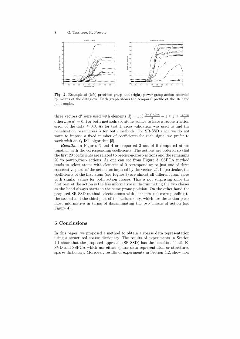
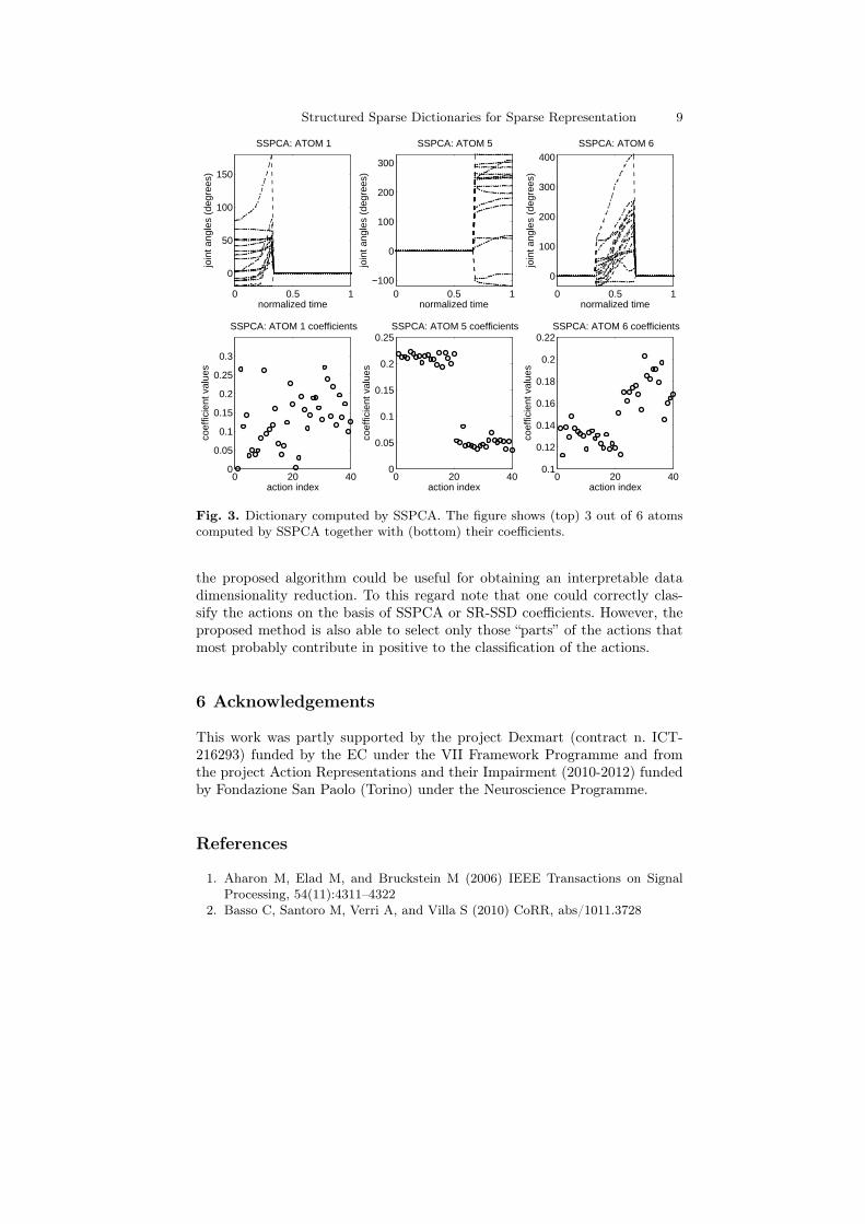
Results. In Figures 3 and 4 are reported 3 out of 6 computed atomstogether with the corresponding coefficients. The actions are ordered so thatthe first 20 coefficients are related to precision-grasp actions and the remaining20 to power-grasp actions. As one can see from Figure 3, SSPCA methodtends to select atoms with elements 6= 0 corresponding to just one of threeconsecutive parts of the actions as imposed by the vectors di. In particular, thecoefficients of the first atom (see Figure 3) are almost all different from zeroswith similar values for both action classes. This is not surprising since thefirst part of the action is the less informative in discriminating the two classesas the hand always starts in the same prone position. On the other hand theproposed SR-SSD method selects atoms with elements > 0 corresponding tothe second and the third part of the actions only, which are the action partsmost informative in terms of discriminating the two classes of action (seeFigure 4).

5 Conclusions

In this paper, we proposed a method to obtain a sparse data representationusing a structured sparse dictionary. The results of experiments in Section4.1 show that the proposed approach (SR-SSD) has the benefits of both K-SVD and SSPCA which use either sparse data representation or structuredsparse dictionary. Moreover, results of experiments in Section 4.2, show how

Structured Sparse Dictionaries for Sparse Representation 9

0 0.5 1

0

50

100

150

normalized time

join

t ang

les

(deg

rees

)

SSPCA: ATOM 1

0 0.5 1−100

0

100

200

300

normalized time

join

t ang

les

(deg

rees

)

SSPCA: ATOM 5

0 0.5 1

0

100

200

300

400

normalized time

join

t ang

les

(deg

rees

)

SSPCA: ATOM 6

0 20 400

0.05

0.1

0.15

0.2

0.25

0.3

action index

coef

ficie

nt v

alue

s

SSPCA: ATOM 1 coefficients

0 20 400

0.05

0.1

0.15

0.2

0.25

action index

coef

ficie

nt v

alue

s

SSPCA: ATOM 5 coefficients

0 20 400.1

0.12

0.14

0.16

0.18

0.2

0.22

action index

coef

ficie

nt v

alue

s

SSPCA: ATOM 6 coefficients

Fig. 3. Dictionary computed by SSPCA. The figure shows (top) 3 out of 6 atomscomputed by SSPCA together with (bottom) their coefficients.

the proposed algorithm could be useful for obtaining an interpretable datadimensionality reduction. To this regard note that one could correctly clas-sify the actions on the basis of SSPCA or SR-SSD coefficients. However, theproposed method is also able to select only those “parts” of the actions thatmost probably contribute in positive to the classification of the actions.

6 Acknowledgements

This work was partly supported by the project Dexmart (contract n. ICT-216293) funded by the EC under the VII Framework Programme and fromthe project Action Representations and their Impairment (2010-2012) fundedby Fondazione San Paolo (Torino) under the Neuroscience Programme.

References

1. Aharon M, Elad M, and Bruckstein M (2006) IEEE Transactions on SignalProcessing, 54(11):4311–4322

2. Basso C, Santoro M, Verri A, and Villa S (2010) CoRR, abs/1011.3728

10 G. Tessitore, R. Prevete

0 0.5 1

−300

−200

−100

0

normalized time

join

t ang

les

(deg

rees

)

SR−SSD: ATOM 1

0 0.5 1

0

100

200

300

400

500

normalized time

join

t ang

les

(deg

rees

)

SR−SSD: ATOM 5

0 0.5 10

50

100

150

200

normalized time

join

t ang

les

(deg

rees

)

SR−SSD: ATOM 6

0 20 40−0.12

−0.1

−0.08

−0.06

−0.04

−0.02

0

action index

coef

ficie

nt v

alue

s

SR−SSD: ATOM 1 coefficients

0 20 400

0.05

0.1

0.15

0.2

action index

coef

ficie

nt v

alue

s

SR−SSD: ATOM 5 coefficients

0 20 400

0.1

0.2

0.3

0.4

0.5

action index

coef

ficie

nt v

alue

s

SR−SSD: ATOM 6 coefficients

Fig. 4. Dictionary computed by SR-SSD. The figure shows (top) 3 out of 6 atomscomputed by SR-SSD together with (bottom) their coefficients.

3. Bredies K and Lorenz D (2008) J Fourier Anal Appl, 14(5-6):813–8374. Chen SS, Donoho DL, and Saunders MA (1998) SIAM Journal on Scientific

Computing, 20(1):33–615. Daubechies I, Defrise M, and De Mol C (2004) Communications on Pure and

Applied Mathematics, 57(11):1413–14576. Engan K, Aase SO, and Husoy JH (1999) In Proc. of ICASSP ’99, 5:2443–2446.

IEEE Computer Society7. Hastie T, Tibshirani R, and Friedman JH (2001) The Elements of Statistical

Learning: Data Mining, Inference, and Prediction. Springer8. Jenatton R, Audibert JY, and Bach F (2009) Structured variable selection with

sparsity-inducing norms. Technical report, arXiv:0904.35239. Jenatton R, Obozinski G, and Bach F (2010) Structured sparse principal com-

ponent analysis. International Conference on AISTATS

10. Micchelli CA and Pontil M (2005) Journal of Machine Learning Research,6:1099–1125

11. Tropp JA (2004) IEEE Trans. Inform. Theory, 50:2231–224212. Vinjamuri R, Lee HN, and Mao ZH (2010) IEEE Trans Biomed Eng, 57(2):284–

29513. Wright J, Ma Y, Mairal J, Sapiro G, Huang TS, and Yan S (2010) Proceedings

of the IEEE, 98(6):1031–104414. Zou H, Hastie T, and Tibshirani R (2004) Sparse Principal Component Anal-

ysis. Journal of Computational and Graphical Statistics, 15