
Spatially Structured Recurrent Modules - arXiv
22
Spatially Structured Recurrent Modules Nasim Rahaman 12 Anirudh Goyal 2 Muhammad Waleed Gondal 1 Manuel Wuthrich 1 Stefan Bauer 1 Yash Sharma 3 Yoshua Bengio 2 Bernhard Sch¨ olkopf 1 Abstract Capturing the structure of a data-generating pro- cess by means of appropriate inductive biases can help in learning models that generalize well and are robust to changes in the input distribution. While methods that harness spatial and tempo- ral structures find broad application, recent work (Goyal et al., 2019) has demonstrated the poten- tial of models that leverage sparse and modular structure using an ensemble of sparingly interact- ing modules. In this work, we take a step towards dynamic models that are capable of simultane- ously exploiting both modular and spatiotemporal structures. We accomplish this by abstracting the modeled dynamical system as a collection of au- tonomous but sparsely interacting sub-systems. The sub-systems interact according to a topol- ogy that is learned, but also informed by the spa- tial structure of the underlying real-world system. This results in a class of models that are well suited for modeling the dynamics of systems that only offer local views into their state, along with corresponding spatial locations of those views. On the tasks of video prediction from cropped frames and multi-agent world modeling from par- tial observations in the challenging Starcraft2 do- main, we find our models to be more robust to the number of available views and better capable of generalization to novel tasks without additional training, even when compared against strong base- lines that perform equally well or better on the training distribution. 1. Introduction Many spatiotemporal complex systems can be abstracted as a collection of autonomous but sparsely interacting sub- * Equal contribution 1 Max Planck Institute for Intelli- gent Systems, T ¨ ubingen 2 Mila, Qu ´ ebec 3 Bethgelab, Univer- sity of T ¨ ubingen. Correspondence to: Nasim Rahaman <[email protected]>. Preprint, work in progress. systems, where sub-systems tend to interact if they are in each others’ local vicinity in some sense. As an illustrative example, consider a grid of traffic intersections, wherein traffic flows from a given intersection to the adjacent ones, and the actions taken by some “agent”, say an autonomous vehicle, may at first only affect its immediate surroundings. Now suppose we want to forecast the future state of the traffic grid (say for the purpose of avoiding traffic jams). There is a spectrum of possible strategies to model the sys- tem at hand. On one end of it lies the most general strategy: namely, one that calls for considering the entirety of all intersections simultaneously to predict the next state of the grid (Figure 1c). The resulting model class can in principle account for interactions between any two intersections, irre- spective of their spatial distance. However, the number of interactions such models must consider does not scale well with the size of the grid, and the strategy might be rendered infeasible for large grids with hundreds of intersections. On the other end of the spectrum is a specialized strategy that involves abstracting the dynamics of each intersection as an autonomous sub-system, and having each sub-system interact only with other sub-systems associated with the four (or more) neighboring intersections (Figure 1c). The interactions may manifest as messages that one sub-system passes to another and possibly contain information about how many vehicles are headed towards which direction, resulting in a collection of message passing entities (i.e., sub- systems) that collectively model the entire grid. By adopting this strategy, one assumes that the immediate future of any given intersection is affected only by the present states of the neighboring intersections, and not some intersection at the opposite end of the grid. The resulting class of models scales well with the size of the grid, but is possibly unable to model certain long-range interactions that could be leveraged to efficiently distribute traffic flow. The spectrum above parameterizes the extent to which the spatial structure of the underlying system being modeled is incorporated into the design of the model. The former extreme ignores spatial structure altogether, resulting in a class of models that can be expressive but whose sample and computational complexity do not scale well with the size of the system. The latter extreme results in a class of arXiv:2007.06533v1 [cs.LG] 13 Jul 2020
-
Upload
khangminh22 -
Category
Documents
-
view
4 -
download
0
Transcript of Spatially Structured Recurrent Modules - arXiv
Spatially Structured Recurrent Modules
Nasim Rahaman 1 2 Anirudh Goyal 2 Muhammad Waleed Gondal 1 Manuel Wuthrich 1 Stefan Bauer 1
Yash Sharma 3 Yoshua Bengio 2 Bernhard Scholkopf 1
Abstract
Capturing the structure of a data-generating pro-cess by means of appropriate inductive biases canhelp in learning models that generalize well andare robust to changes in the input distribution.While methods that harness spatial and tempo-ral structures find broad application, recent work(Goyal et al., 2019) has demonstrated the poten-tial of models that leverage sparse and modularstructure using an ensemble of sparingly interact-ing modules. In this work, we take a step towardsdynamic models that are capable of simultane-ously exploiting both modular and spatiotemporalstructures. We accomplish this by abstracting themodeled dynamical system as a collection of au-tonomous but sparsely interacting sub-systems.The sub-systems interact according to a topol-ogy that is learned, but also informed by the spa-tial structure of the underlying real-world system.This results in a class of models that are wellsuited for modeling the dynamics of systems thatonly offer local views into their state, along withcorresponding spatial locations of those views.On the tasks of video prediction from croppedframes and multi-agent world modeling from par-tial observations in the challenging Starcraft2 do-main, we find our models to be more robust to thenumber of available views and better capable ofgeneralization to novel tasks without additionaltraining, even when compared against strong base-lines that perform equally well or better on thetraining distribution.
1. IntroductionMany spatiotemporal complex systems can be abstractedas a collection of autonomous but sparsely interacting sub-
*Equal contribution 1Max Planck Institute for Intelli-gent Systems, Tubingen 2Mila, Quebec 3Bethgelab, Univer-sity of Tubingen. Correspondence to: Nasim Rahaman<[email protected]>.
Preprint, work in progress.
systems, where sub-systems tend to interact if they are ineach others’ local vicinity in some sense. As an illustrativeexample, consider a grid of traffic intersections, whereintraffic flows from a given intersection to the adjacent ones,and the actions taken by some “agent”, say an autonomousvehicle, may at first only affect its immediate surroundings.Now suppose we want to forecast the future state of thetraffic grid (say for the purpose of avoiding traffic jams).
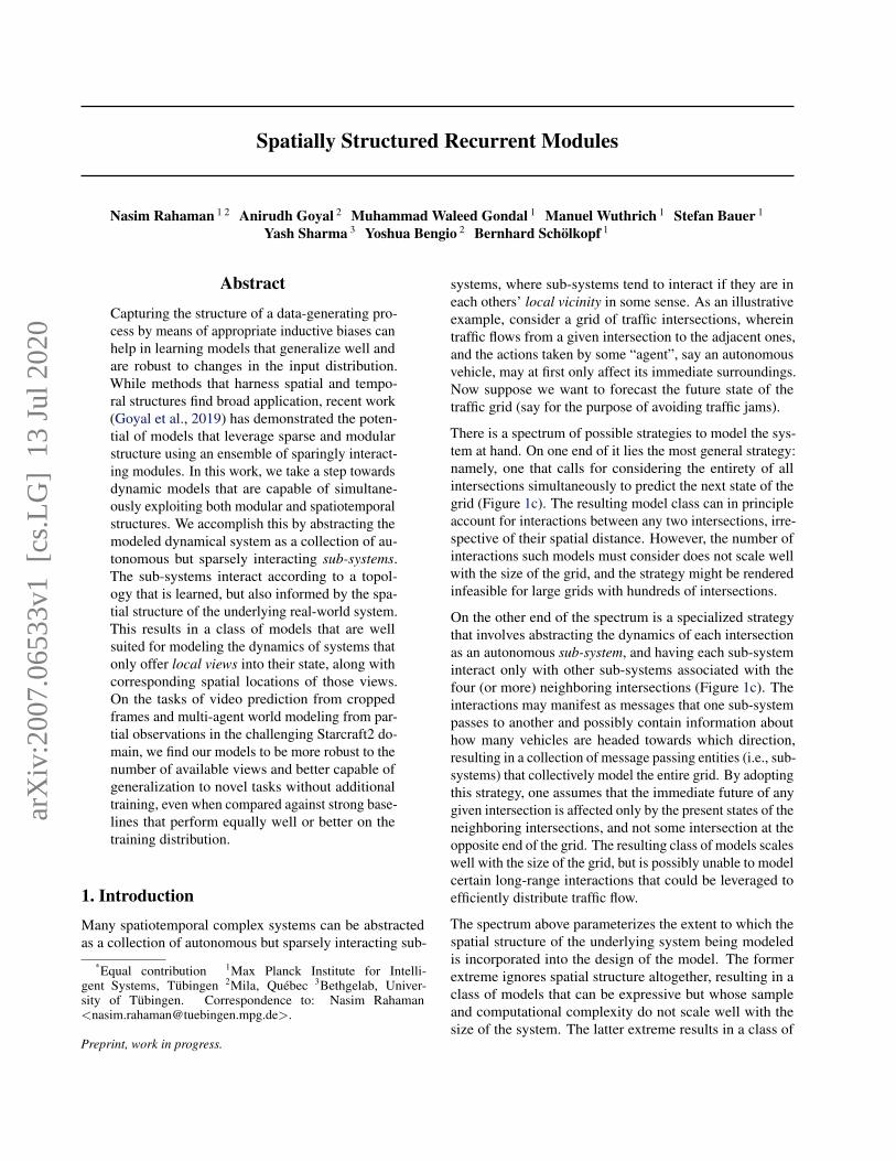
There is a spectrum of possible strategies to model the sys-tem at hand. On one end of it lies the most general strategy:namely, one that calls for considering the entirety of allintersections simultaneously to predict the next state of thegrid (Figure 1c). The resulting model class can in principleaccount for interactions between any two intersections, irre-spective of their spatial distance. However, the number ofinteractions such models must consider does not scale wellwith the size of the grid, and the strategy might be renderedinfeasible for large grids with hundreds of intersections.
On the other end of the spectrum is a specialized strategythat involves abstracting the dynamics of each intersectionas an autonomous sub-system, and having each sub-systeminteract only with other sub-systems associated with thefour (or more) neighboring intersections (Figure 1c). Theinteractions may manifest as messages that one sub-systempasses to another and possibly contain information abouthow many vehicles are headed towards which direction,resulting in a collection of message passing entities (i.e., sub-systems) that collectively model the entire grid. By adoptingthis strategy, one assumes that the immediate future of anygiven intersection is affected only by the present states of theneighboring intersections, and not some intersection at theopposite end of the grid. The resulting class of models scaleswell with the size of the grid, but is possibly unable to modelcertain long-range interactions that could be leveraged toefficiently distribute traffic flow.
The spectrum above parameterizes the extent to which thespatial structure of the underlying system being modeledis incorporated into the design of the model. The formerextreme ignores spatial structure altogether, resulting in aclass of models that can be expressive but whose sampleand computational complexity do not scale well with thesize of the system. The latter extreme results in a class of
arX
iv:2
007.
0653
3v1
[cs
.LG
] 1
3 Ju
l 202
0
S2RM: Spatially Structured Recurrent Modules
(a) Fully localized sub-systems. (b) Middle ground. (c) Single, monolithic system.
Figure 1. A schematic representation of the spectrum of modeling strategies. Solid arrows with speech bubbles denote (dynamic) messagesbeing passed between sub-systems (dotted arrows denote the lack thereof). Gist: on the one end of the spectrum, (Figure 1a), we have thestrategy of abstracting each intersection as a sub-system that interact with neighboring sub-systems. On the other end of the spectrum(Figure 1c) we have the strategy of modeling the entire grid with one monolithic system. The middle ground (Figure 1b) we exploreinvolves letting the model develop a notion of locality by (say) abstracting entire avenues with a single sub-system.
models that can scale well, but its adequacy (in terms ofexpressivity) is contingent on a predefined notion of locality(in the example above: the immediate four-neighborhood ofan intersection). In this work, we aim to explore a middle-ground between the two extremes: namely, by proposinga class of models that does leverage the spatial structure,but by developing a notion of locality instead of relyingon a predefined one (Figure 1b). Reconsidering the trafficgrid example: the proposed strategy results in a model thatcan potentially learn to abstract (say) entire avenues with asingle sub-system. The interactions between intersectionsare therefore replaced by those between avenues, resultingin a scheme where a single sub-system might account forevents that are spatially distant (such as those in the oppositeends of an avenue), but two events that are spatially closertogether (such as those on two adjacent avenues of the samestreet, where streets run perpendicular to avenues) might beaccounted for by different sub-systems.
To implement this scheme, we will model the sub-systemsas independent recurrent neural networks (RNNs) that in-teract sparsely via a bottleneck of attention (Goyal et al.,2019), but extend this idea along two salient dimensions.First, we relax the assumption that the interaction topol-ogy between sub-systems (i.e., RNNs) is all-to-all, in thesense that all sub-systems are allowed to interact with allother sub-systems. We achieve this by learning to embedeach sub-system in an embedding space endowed with ametric, and attenuate the interaction between two given sub-systems by their distance in this space (i.e., sub-systemstoo far away from each other in this space are not allowedto interact). Second, instead of assuming that the entiresystem is perceived simultaneously, we only assume accessto local (partial) observations alongside with the associatedspatial locations, resulting in a setting that partially resem-bles that of Eslami et al. (2018). Expressed in the languageof the example above: we do not expect a birds eye viewof the traffic grid, but only (say) LIDAR observations from
autonomous vehicles at known GPS coordinates, or videostreams from traffic cameras at known locations. The spatiallocation associated with an observation plays a crucial rolein the proposed architecture in that we map it to the embed-ding space of sub-systems and address the correspondingobservation only to sub-systems whose embeddings lie inclose vicinity. Likewise, to predict future observations ata queried spatial location, we again map said location tothe embedding space and poll the states of sub-systems sit-uated nearby. The result is a model that can learn whichspatial locations are to be associated with each other and beaccounted for by the same sub-system. As an added plus,the parameterization we obtain is not only agnostic to thenumber of available observations and query locations, butalso to the number of sub-systems.
To evaluate the proposed model, we choose a problem set-ting where (a) the task is composed of different sub-systemsor processes that locally interact both spatially and tempo-rally, and (b) the environment offers local views into itsstate paired with their corresponding spatial locations. Thechallenge here lies in building and maintaining a consistentrepresentation of the global state of the system given only aset of partial observations. To succeed, a model must learnto efficiently capture the available observations and placethem in appropriate spatial context. The first problem weconsider is that of video prediction from crops, analogousto that faced by visual systems of many animals: givena set of small crops of the video frames centered aroundstochastically sampled pixels (corresponding to where thefovea is focused), the task is to predict the content of a croparound any queried pixel position at a future time. Thesecond problem is that of multi-agent world modeling frompartial observations in spatial domains, such as the chal-lenging Starcraft2 domain (Samvelyan et al., 2019; Vinyalset al., 2017). The task here is to model the dynamics ofthe global state of the environment given local observationsmade by cooperating agents and their corresponding actions.
S2RM: Spatially Structured Recurrent Modules
Importantly and unlike prior work (Sun et al., 2019), ourparameterization is agnostic to the number of agents in theenvironment, which can be flexibly adjusted on the fly asnew agents become available or existing agents retire. Thisis beneficial for generalization in settings where the numberof agents during training and testing are different.
Contributions. (a) We propose a new class of models,which we call Spatially Structured Recurrent Modules orS2RMs, which perform attention-driven spatially local mod-ular computations. (b) We evaluate S2RMs (along with sev-eral strong baselines) on a selection of challenging problemsto find that S2RMs are robust to the number of availableobservations and can generalize to novel tasks.
2. Problem StatementIn this section, we build on the intuition from the previoussection to formally specify the problem we aim to approachwith the methods described in the later sections.
Let X be a metric space, O some set of possible observa-tions, and OX a set of mappings X → O. Now, considerthe evolution function of a discrete-time dynamical system:
φ : Z×OX → OX satisfying (1)φ(0, o) = o where o ∈ OX andφ(t2, φ(t1, o)) = φ(t1 + t2, o) for t1, t2 ∈ Z
Informally, o can be interpreted as the world state of thesystem; together with a spatial location x ∈ X , it gives thelocal observation O = o(x) ∈ O. Given an initial worldstate o, the mapping φ(t, o) yields the world state at some(future) time t, thereby characterizing the dynamics of thesystem (which might be stochastic).
While the above class of dynamical systems is fairly general,we now place a crucial restriction: namely, that for any pairof space-time events (t1,x1) ∈ (Z × X ) and (t2,x2) andgiven any initial state o0 ∈ OX , there exists a finite C > 0such that the observation φ(t1, o0)(x1) can influence theobservation φ(t2, o0)(x2) only if t2 ≥ t1 and dX (x1,x2) ≤C · (t2− t1), where dX is the metric on X . This assumptioninduces a notion of spatio-temporal locality by imposingthat the effect of any given event can only propagate at afinite speed, where the latter is upper bounded by C.
In this work, we are concerned with modelling systems thatare subject to the above restriction. Assuming the systemsatisfies said restriction, we have the following
Problem: At every time step t = 0, ..., T , we are given a setof positions {xa
t }Aa=1 and the corresponding observations{Oa
t }Aa=1, where Oat := φ(t, o0)(xa) for some initial world
state o0. The task is to infer the world state φ(t′, o0) at somefuture time-step t′ > T .
In the traffic grid example of Section 1, one could imagine
a as indexing traffic cameras or autonomous vehicles (i.e.,observers), xa
t as the GPS coordinates of observer a, and Oat
as the corresponding sensor feed (e.g. LIDAR observationsor video streams from vehicles or traffic cameras).
3. Modelling AssumptionsGiven the problem in Section 2, we now constrain it byplacing certain structural assumptions. These assumptionswill ultimately inform the inductive biases we select forthe model (proposed in Section 4); nevertheless, we remarkbeforehand that as with any inductive bias, their applicabilityis subject to the properties of the system being modeled andthe objectives1 being optimized.
Recurrent Dynamics Modeling. While there exist multi-ple ways of modeling dynamical systems, we shall focus onrecurrent neural networks (RNNs). Typically, RNN-baseddynamics models are expressed as functions of the form:
ht+1 = F (Ot,ht) Ot = D(ht) (2)
where Ot is the observation at time t ∈ Z, and ht+1 isthe hidden state of the model. F can be thought of asthe parameterized forward-evolution function the hiddenstate h conditioned on the observation O, whereas D is adecoder that maps the hidden state to observations. Here,the evolution function of the modelled dynamical system(as defined in Equation 1) can be obtained by rolling out theforward-evolution function in time.
Decomposition into Sub-systems. Without loss of gener-ality, one may assume that the dynamical system φ definedin Equation 1 can be decomposed into constituent systems(φ1, φ2, ..., φM ), such that the interaction between all pairsof sub-systems (φi, φj) satisfy some criterion. Now, thestrength of this assumed criterion lies on a spectrum. Onone end of the spectrum is the case where such a criterion isnon-existent, i.e., no such decomposition is assumed and fullgenerality is restored; this is the modeling assumption madewhen using conventional recurrent models like GRUs (Choet al., 2014), LSTMs (Hochreiter & Schmidhuber, 1997)and vanilla RNNs. On the other end of the spectrum lies asetting where the decomposition is required to be such thatsub-systems do not interact, i.e., φi and φj have independentdynamics (Li et al., 2018). Goyal et al. (2019) explore amiddle ground, where the interaction between sub-systems(φi, φj) are possible but constrained. In particular, theyinvestigate a setting where the sub-systems are assumedto interact sparsely, and the interaction pattern (i.e., whichsub-systems interact with which others) is dynamic and maydepend on the world state o. In this work, we adopt theassumption of sparsely interacting sub-systems, but subjectthe interaction pattern to an additional spatial constraint.
1E.g. generalization, sample complexity, robustness, etc.
S2RM: Spatially Structured Recurrent Modules
Encoder Decoder
Input Attention
Output Attention
Positional Embedding
Positional Embedding
Observation Location
Observation at Location
Query Location
Predicted Observation at Queried Location
Set of Interacting RNNs
F1
F2
F3
F4
Figure 2. Schematic representation of the proposed architecture.
Local Interactions Between Sub-systems. In addition toassuming dynamic sparse interactions between sub-systems,we also assume that a given sub-system φj may preferen-tially interact with another given sub-system φi. Intuitively,one may think of φj as lying in vicinity of φi. This naturallyleads us to a notion of topology over sub-systems, one wheresub-systems situated in each other’s local neighborhood areless constrained in their interactions. In the next section,we will discuss how we model this topology by associatingeach sub-system φi with a learned embedding pi in an ex-isting metric space, which we will call S . Subsequently, theaffinity of sub-system φi to interact with another sub-systemφj will be quantified by a similarity measure Z, such thatZ(pi,pj) is large if φi and φj prefer to interact.
Locality of Observations. Recall from Section 2 that theobservations available to the model respect a notion ofspatio-temporal locality. However, this notion of localityis distinct from the one between sub-systems (induced viaZ), and one important modeling decision is how the twoshould interact. We propose to embed the position x ∈ Xassociated with an observation O to the metric space ofsub-systems S via a continuous and one-to-one mappingP : X → S , which allows us to match the observation O toall sub-systems φm in the vicinity of P (x) ∈ S , i.e., whereZ(P (x),pm) is sufficiently large. Likewise, the same sub-systems φm are polled if the model is queried for a predic-tion at x. On a high level, this results in a scheme whereeach subsystem φm can account for observations made ata set of positions Xm ⊂ X , which we call its enclave. Inparticular, the enclaves Xi and Xj corresponding to sub-systems φi and φj may overlap, and we do not constrain thedistance between two given points in Xm to be small.
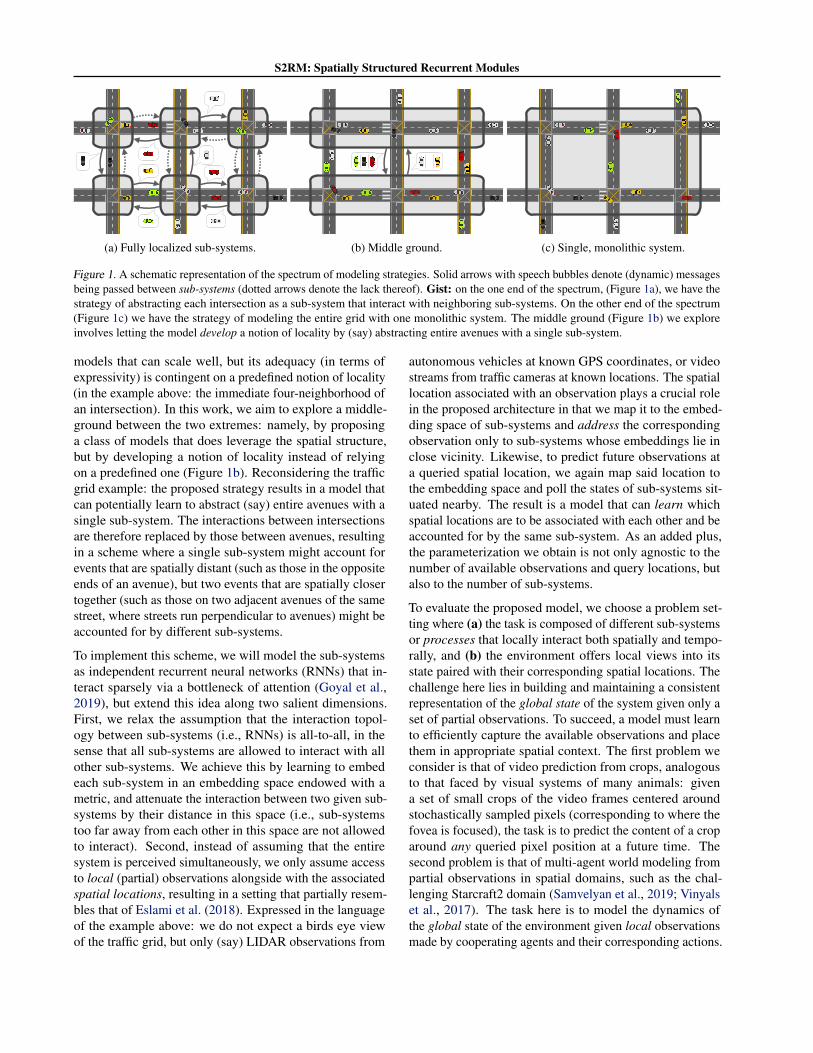
4. Proposed ModelInformed2 by the model assumptions detailed in the previoussection, we now proceed to describe the proposed model –Spatially Structured Recurrent Modules or S2RM – whichcomprise the following components (Figure 2):
Model Inputs. Recall from Section 2 that we have for ev-ery time step t = 0, ..., T a set of tuples of positions and
2In doing so, we use the assumptions merely as guiding princi-ples; we do not claim that we infer e.g. the true decomposition ofthe ground-truth system, even if all assumptions are satisfied.
observations {(xat ,O
at )}Aa=1 where xa
t ∈ X and Oat ∈ O
for all t and a. To simplify, we assume that X ⊂ Rn, anddenote by xi the i-th component of the vector x ∈ X . En-coder. The encoder E is a parameterized function mappingobservations O to a corresponding vector representatione = E(O). Here, E processes all observations in parallelacross t and a to yield representations eat .
Positional Embedding. The positional embedding P is afixed mapping from X to S. We choose S to be the unitsphere in d-dimensions, d being a multiple of 2n, and thepositional encoder as the following function:
P (x) = s/‖s‖ ∈ S where (3)s2i+m = sin (xm/10000i) s2i+1+m = cos (xm/10000i) (4)
with m = 1, ..., n and i = 1, ..., d/2n. While the abovefunction is commonly used (Vaswani et al., 2017), otherchoices might also be viable. Accommodating a slight abuseof notation, we will refer to P (x) as s and P (xa
t ) as sat .
Set of Interacting RNNs. To model the dynamics of theworld state, we use a set of M independent RNN modules(like in Goyal et al. (2019)), which we denote as {Fm}Mm=1.To each Fm, we associate an embedding vector pm ∈ S,where all {pm}Mm=1 are learnable parameters. On a highlevel, RNNs Fm interact with each other via an inter-cellattention, and with the input representations eat via inputattention. More precisely, at a given time step t, each Fm
expects an input umt , together with an aggregated hidden
state hmt and optionally a memory state cmt to yield the
hidden and memory states at the next time step:
(hmt+1, c
mt+1) = Fm(um
t , hmt , c
mt ) (5)
where the input umt results from the input attention and
hmt from the inter-cell attention (both described below). If
available, the memory state cmt resembles the cell state inan LSTM (Hochreiter & Schmidhuber, 1997).
Input Attention. Similar to MHDPA (multi-head dot-product attention, Vaswani et al. (2017)), the input atten-tion mechanism is a mapping between sets: namely, fromthat of observation encodings {eat }Aa=1 to that of RNN in-puts {um
t }Mm=1. In what follows, we use the einsum nota-tion3 to succintly describe the exact mechanism. But be-fore that, we define the truncated spherical Gaussian kernel(Fasshauer, 2011) to quantify the similarity between twopoints p, s ∈ S:
Z(p, s) =
{exp [−2ε(1− p · s)], if p · s ≥ τ0, otherwise
(6)
where ε ∈ R+ and τ ∈ [−1, 1) are hyper-parameters (kernelbandwidth and truncation parameter, respectively), and
3Indices not appearing on both sides of an equation are summedover; this is implemented as einsum in most DL frameworks.
S2RM: Spatially Structured Recurrent Modules
0 ≤ Z ≤ 1 since p and s are unit vectors. Now, we usek to index the attention heads, d to index the dimensionof the key and query vectors, and denote with eai the i-thcomponent of eat and with hmj the j-th component of hm
t .Given learnable parameters Θ(K), Θ(Q), Θ(V ), we obtain:
Qakd = eaiΘ(Q)ikd Kmkd = hmjΘ
(K)jkd (7)
Vakv = eaiΘ(V )ikv Wmak = QakdKmkd (8)
Wmak = sma(Wmak) W (L)ma = Z(pm, sa) (9)
Wmak = W (L)ma Wmak um(kv) = WmakVakv (10)
where: sma denotes softmax along the a-dimension, W (L)
is what we will call the local weights, we omit the time sub-script in sa for notational clarity, and um(kv) is the (kv)-thcomponent of a vector um. Finally, we obtain the compo-nents umi of RNN inputs um
t via a gating operation:
umi = G(inp)m · bmi + (1−G(inp)
m ) · umi (11)
where the gating weight G(inp)m ∈ (0, 1) is obtained by pass-
ing umi and bmi = W(L)ma eai through a two-layer MLP with
sigmoidal output (in parallel across m). Now, observe thatby weighting the MHDPA attention outputs (W in Equa-tion 10) by the kernel Z (via W (L)), we construct a schemewhere the interaction between input Oa
t and RNN Fm isallowed only if the embedding sat of the corresponding po-sition xa
t has a large enough cosine similarity (≥ τ ) tothe embedding pm of Fm. This partially implements theassumption of Locality of Observation detailed in Section 3.
Inter-cell Attention. The inter-cell attention maps the hid-den states of each RNN {hm
t }Mm=1 to the set of aggregatedhidden states {hm
t }Mm=1, thereby enabling interaction be-tween the RNNs Fm. While its mechanism is identicalto that of the input attention, we formulate it below forcompleteness. To proceed, we denote with hli the i-th com-ponent of hl
t (in addition to the notation introduced beforeEquation 7), and take Φ(Q), Φ(K) and Φ(V ) to be learnableparameters. We have:
Qmkd = hmjΦ(Q)jkd Klkd = hliΦ
(K)ikd (12)
Vlkv = hliΦ(V )ikv Wmlk = QmkdKlkd (13)
Wmlk = sml(Wmlk) W(L)ml = Z(pm,pl) (14)
Wmlk = WmlkW(L)ml hm(kv) = WmlkVlkv (15)
where hm(kv) is the (kv)-th component of a vector hm.Finally, the j-th component hmj of the aggregated hiddenstate hm
t in Equation 5 is given by a gating operation:
hmj = G(ic)m · cmj + (1−G(ic)
m ) · hmj (16)
where the gating weight G(ic)m ∈ (0, 1) is obtained by pass-
ing hmj and cmj = W(L)ml hlj through a two-layer MLP
with sigmoid output (in parallel across m). The weightingby Z (in Equation 15, left) ensures that the interaction isconstrained to be only between RNNs whose embeddings inS are similar enough, thereby implementing the assumptionof Local Interactions between Sub-systems in Section 3.
Output Attention. The output attention mechanism to-gether with the decoder (described below) serve as an ap-paratus to evaluate the world state modeled (implicitly) bythe set of RNNs ({Fm}Mm=1) at time t + 1 (for one-stepforward models). Given a query location xq ∈ X and itscorresponding embedding sq = P (xq) ∈ S, the output at-tention mechanism polls the RNNs Fm whose embeddingspm are similar enough to sq, as measured by the kernel Z.Denoting hmj the j-th component of hm
t+1, we have:
dqj = Z(sq,pm)hmj (17)
where dqj can be interpreted as the j-th component of thevector dq
t+1 associated with the query location xq .
Decoder. The decoder D is a parameterized function thatpredicts the observation Oq
t+1 ∈ O at xq given the repre-sentation dq
t+1 from the output attention.
This concludes the description of the generic architecture,which allows for flexibility in the choice of the RNN archi-tecture (i.e., the internal architecture of Fm). In practice,we find Gated Recurrent Units (GRUs) (Cho et al., 2014)to work well, and call the resulting model Spatially Struc-tured GRU or S2GRU. Moreover, Relational Memory Cores(RMCs) (Santoro et al., 2018) also profit from our architec-ture (with a minor modification detailed in Appendix B.3),and we refer to the resulting model as S2RMC.
5. Related WorkProblem Setting. Recall that the problem setting we con-sider is one where the environment offers local (partial)views into its global state paired with the correspondingspatial locations. With Generative Query Networks (GQNs),Eslami et al. (2018) investigate a similar setting where the2D images of 3D scenes are paired with the correspondingviewpoint (camera position, yaw, pitch and roll). Given thatGQNs are feedforward models, they do not consider thedynamics of the underyling scene and as such cannot beexpected to be consistent over time (Kumar et al., 2018).Singh et al. (2019) and Kumar et al. (2018) propose variantsthat are temporally consistent, but unlike us, they do notfocus on the problem of modeling the forward dynamics.
Modularity. Modularity has been a recurring topic in thecontext of meta-learning (Alet et al., 2018; Bengio et al.,2019; Ke et al., 2019), sequence modeling (Henaff et al.,2016; Goyal et al., 2019; Li et al., 2018) and beyond (Jacobset al., 1991; Shazeer et al., 2017; Parascandolo et al., 2017).However, unlike prior work, we integrate modularity and
S2RM: Spatially Structured Recurrent Modules
spatio-temporal structure in a unified framework.
Spatial Attention. Mechanisms for spatial attention havebeen well studied (Jaderberg et al., 2015; Wang et al., 2017;Zhang et al., 2018; Parmar et al., 2018), but they typicallyoperate on image pixels. Our setting is more general in thesense that we do not necessarily require that the world stateof the underlying system be represented by images.
Attention Mechanisms and Information Flow. Attentionmechanisms have been used to attenuate the flow of infor-mation between components of the network, e.g. in NTMs(Graves et al., 2014), DNCs (Graves et al., 2016), RMCs(Santoro et al., 2018), SAB (Ke et al., 2018) and GraphAttention Networks (Velickovic et al., 2017; Battaglia et al.,2018). Our work contributes to this body of literature.
6. ExperimentsIn this section, we present a selection of experiments toempirically evaluate S2RMs and gauge their performanceagainst strong baselines on two data domains. We proceedas follows: in Section 6.1 we introduce the baselines, fol-lowed by experimental results on a video prediction task(Section 6.2) and on the multi-agent world modeling task inthe challenging Starcraft2 domain (Section 6.3). Additionalresults and supporting plots can be found in Appendix C.
6.1. Baseline Methods
To draw fair comparisons, we require a baseline architec-ture that is agnostic to the number of observations A, isinvariant to the ordering of {(xa
t ,Oat )}Aa with respect to a
and features a querying mechanism to extract a predictedobservation Oq
t′ at a given query location xq in a futuretime-step t′ > t. Fortunately, it is possible to obtain aperformant class of models fulfilling our requirements byextending prior work on Generative Query Networks orGQNs (Eslami et al., 2018). The resulting model has threecomponents:
Encoder. At a given timestep t, the encoder E jointly mapsthe embedding sat ∈ S of the position xa
t ∈ X and thecorresponding observations Oa
t to encodings eat , which arethen summed over a to obtain an aggregated representation:
rt =
A∑a=1
E(Oat , s
at ) (18)
The additive aggregation scheme we use is well knownfrom prior work (Santoro et al., 2017; Eslami et al., 2018;Garnelo et al., 2018) and makes the model agnostic to Aand to permutations of (xa
t ,Oat ) over a. The encoder E is
a seven-layer CNN with residual layers, and the positionalembedding sat is injected after the second convolutionallayer via concatenation with the feature tensor. The exact
architectures can be found in Appendices B.1 and B.2.
RNN. The aggregated representation rt is used as an inputto a RNN model F as following:
ht+1, ct+1 = F (rt,ht, ct) (19)
where ht and ct are hidden and memory states of the RNNF respectively. We experiment with various RNN mod-els, including LSTMs (Hochreiter & Schmidhuber, 1997),RMCs (Santoro et al., 2018) and Recurrent IndependentMechanisms (RIMs) (Goyal et al., 2019).
As a sanity check, we also show results with a Time Trav-elling Oracle (TTO), which has access to rt+1 (but at timestep t), and produces ht+1 = FTTO(rt+1) with a two layerMLP FTTO. TTO therefore does not model the dynamics,but merely verifies that the additive aggregation scheme(Equation 18) and the querying mechanism (Equation 20)are sufficient for the task at hand.
Decoder. Given the embedding sq of the query position xq ,the decoderD predicts the corresponding observation Oq
t+1:
Oqt+1 = D(ht+1, s
q) (20)
We parameterize D with a deconvolutional network withresidual layers, and inject the positional embedding of thequery sq after a single convolutional layer by concatenatingwith the layer features (see Appendices B.1 and B.2).
The architecture described above therefore extends theframework of GQNs by predicting the forward dynamicsof the aggregated representation; nevertheless, we do notconsider it a novel contribution of this work.
6.2. Video Prediction from Crops
Task Description. We consider the problem of predictingthe future frames of simulated videos of balls bouncing ina closed box (Miladinovic et al., 2019), given only cropsfrom the past video frames which are centered at knownpixel positions. Using the notation introduced in Section 2:at every time step t, we sample A = 10 pixel positions{xa
t }10a=1 from the t-th full video frame ot of size 48× 48.Around the sampled central pixel positions xa
t , we extract11× 11 crops, which we use as the local observations Oa
t .The task now is to predict 11× 11 crops Oq
t′ correspondingto query central pixel positions xq
t′ at a future time-stept′ > t. Observe that at any given time-step t, the model hasaccess to at most 52% of the global video frame assumingthat the crops never overlap (which is rather unlikely).
Dataset. We train all models on a training dataset of 20Kvideo sequences with 100 frames of 3 balls bouncing in anarena of size 48× 48. We also include an additional fixedball in the center to make the task more challenging. We useanother 1K video sequences of the same length and the same
S2RM: Spatially Structured Recurrent Modules
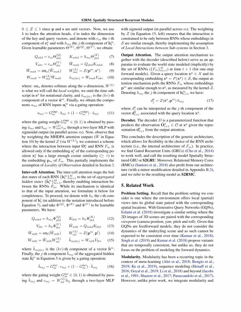
Figure 3. Rollouts (OOD) with 5 bouncing balls, from top to bottom: ground-truth, S2GRU, RIMs, RMC, LSTM. Note that all modelswere trained on sequences with 3 bouncing balls, and the global state was reconstructed by stitching together 11× 11 patches from themodels (queried on a 4× 4 grid). Gist: S2GRU succeeds at keeping track of all bouncing balls over long rollout horizons (25 frames).
1 2 3 4 5 6Number of Bouncing Balls
0.70
0.75
0.80
0.85
0.90
0.95
1.00
Bina
ry F
1-Sc
ore
Training Distr.S2GRU*TTORMCLSTMRIMS
1 2 3 4 5 6Number of Bouncing Balls
0.75
0.80
0.85
0.90
0.95
1.00
Bala
nced
Acc
urac
y
Training Distr.S2GRU*TTORMCLSTMRIMS
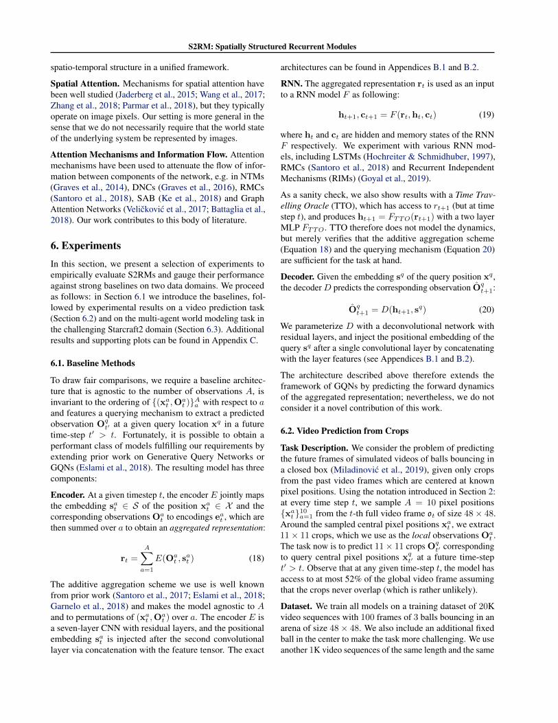
Figure 4. Performance metrics on OOD one-step forward predic-tion task. Gist: S2GRU outperforms all RNN baselines OOD.
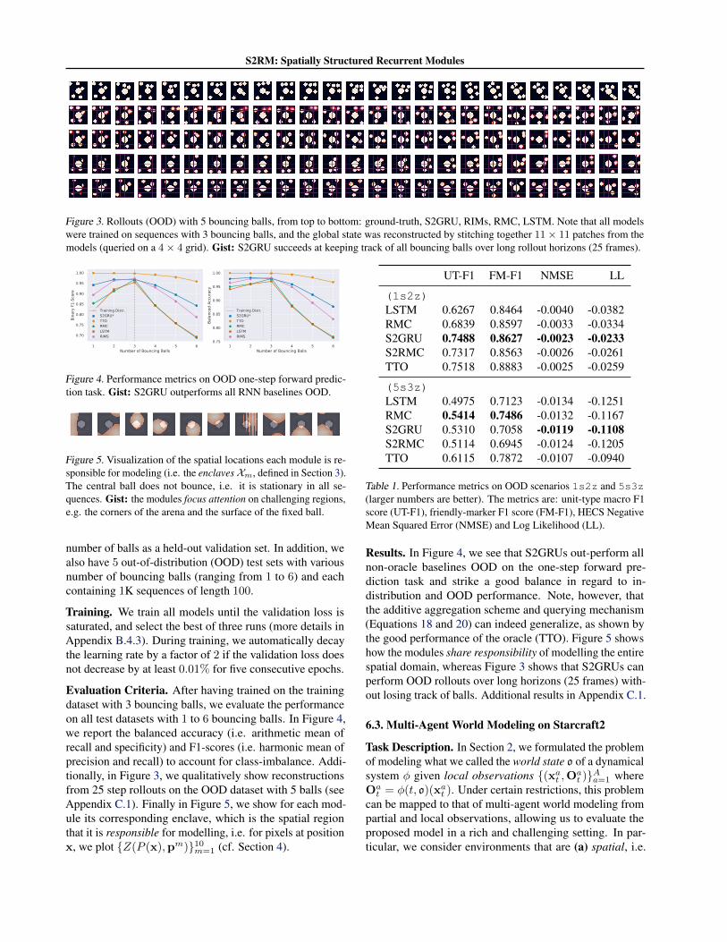
Figure 5. Visualization of the spatial locations each module is re-sponsible for modeling (i.e. the enclavesXm, defined in Section 3).The central ball does not bounce, i.e. it is stationary in all se-quences. Gist: the modules focus attention on challenging regions,e.g. the corners of the arena and the surface of the fixed ball.
number of balls as a held-out validation set. In addition, wealso have 5 out-of-distribution (OOD) test sets with variousnumber of bouncing balls (ranging from 1 to 6) and eachcontaining 1K sequences of length 100.
Training. We train all models until the validation loss issaturated, and select the best of three runs (more details inAppendix B.4.3). During training, we automatically decaythe learning rate by a factor of 2 if the validation loss doesnot decrease by at least 0.01% for five consecutive epochs.
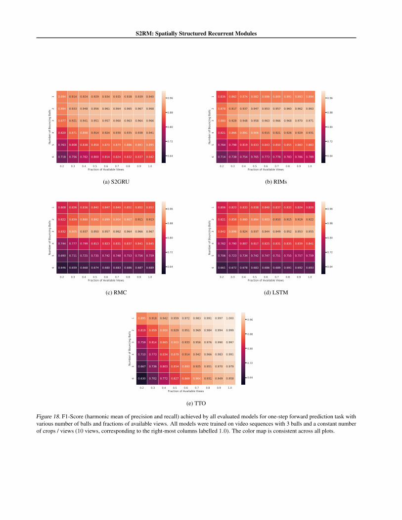
Evaluation Criteria. After having trained on the trainingdataset with 3 bouncing balls, we evaluate the performanceon all test datasets with 1 to 6 bouncing balls. In Figure 4,we report the balanced accuracy (i.e. arithmetic mean ofrecall and specificity) and F1-scores (i.e. harmonic mean ofprecision and recall) to account for class-imbalance. Addi-tionally, in Figure 3, we qualitatively show reconstructionsfrom 25 step rollouts on the OOD dataset with 5 balls (seeAppendix C.1). Finally in Figure 5, we show for each mod-ule its corresponding enclave, which is the spatial regionthat it is responsible for modelling, i.e. for pixels at positionx, we plot {Z(P (x),pm)}10m=1 (cf. Section 4).
UT-F1 FM-F1 NMSE LL
(1s2z)LSTM 0.6267 0.8464 -0.0040 -0.0382RMC 0.6839 0.8597 -0.0033 -0.0334S2GRU 0.7488 0.8627 -0.0023 -0.0233S2RMC 0.7317 0.8563 -0.0026 -0.0261TTO 0.7518 0.8883 -0.0025 -0.0259
(5s3z)LSTM 0.4975 0.7123 -0.0134 -0.1251RMC 0.5414 0.7486 -0.0132 -0.1167S2GRU 0.5310 0.7058 -0.0119 -0.1108S2RMC 0.5114 0.6945 -0.0124 -0.1205TTO 0.6115 0.7872 -0.0107 -0.0940
Table 1. Performance metrics on OOD scenarios 1s2z and 5s3z(larger numbers are better). The metrics are: unit-type macro F1score (UT-F1), friendly-marker F1 score (FM-F1), HECS NegativeMean Squared Error (NMSE) and Log Likelihood (LL).
Results. In Figure 4, we see that S2GRUs out-perform allnon-oracle baselines OOD on the one-step forward pre-diction task and strike a good balance in regard to in-distribution and OOD performance. Note, however, thatthe additive aggregation scheme and querying mechanism(Equations 18 and 20) can indeed generalize, as shown bythe good performance of the oracle (TTO). Figure 5 showshow the modules share responsibility of modelling the entirespatial domain, whereas Figure 3 shows that S2GRUs canperform OOD rollouts over long horizons (25 frames) with-out losing track of balls. Additional results in Appendix C.1.
6.3. Multi-Agent World Modeling on Starcraft2
Task Description. In Section 2, we formulated the problemof modeling what we called the world state o of a dynamicalsystem φ given local observations {(xa
t ,Oat )}Aa=1 where
Oat = φ(t, o)(xa
t ). Under certain restrictions, this problemcan be mapped to that of multi-agent world modeling frompartial and local observations, allowing us to evaluate theproposed model in a rich and challenging setting. In par-ticular, we consider environments that are (a) spatial, i.e.
S2RM: Spatially Structured Recurrent Modules
0.0 0.2 0.4 0.6 0.8Agent Drop Probability
0.3
0.4
0.5
0.6
0.7
Unit
Type
(Mac
ro) F
1-Sc
ore
S2GRU*S2RMC*TTORMCLSTM
0.0 0.2 0.4 0.6 0.8Agent Drop Probability
0.55
0.60
0.65
0.70
0.75
0.80
Frie
ndly
Mar
ker F
1-Sc
ore
S2GRU*S2RMC*TTORMCLSTM
0.0 0.2 0.4 0.6 0.8Agent Drop Probability
0.016
0.014
0.012
0.010
0.008
0.006
HECS
Neg
ativ
e M
SE
S2GRU*S2RMC*TTORMCLSTM
0.0 0.2 0.4 0.6 0.8Agent Drop Probability
0.45
0.40
0.35
0.30
0.25
0.20
0.15
0.10
0.05
Log
Likel
ihoo
d
S2GRU*S2RMC*TTORMCLSTM
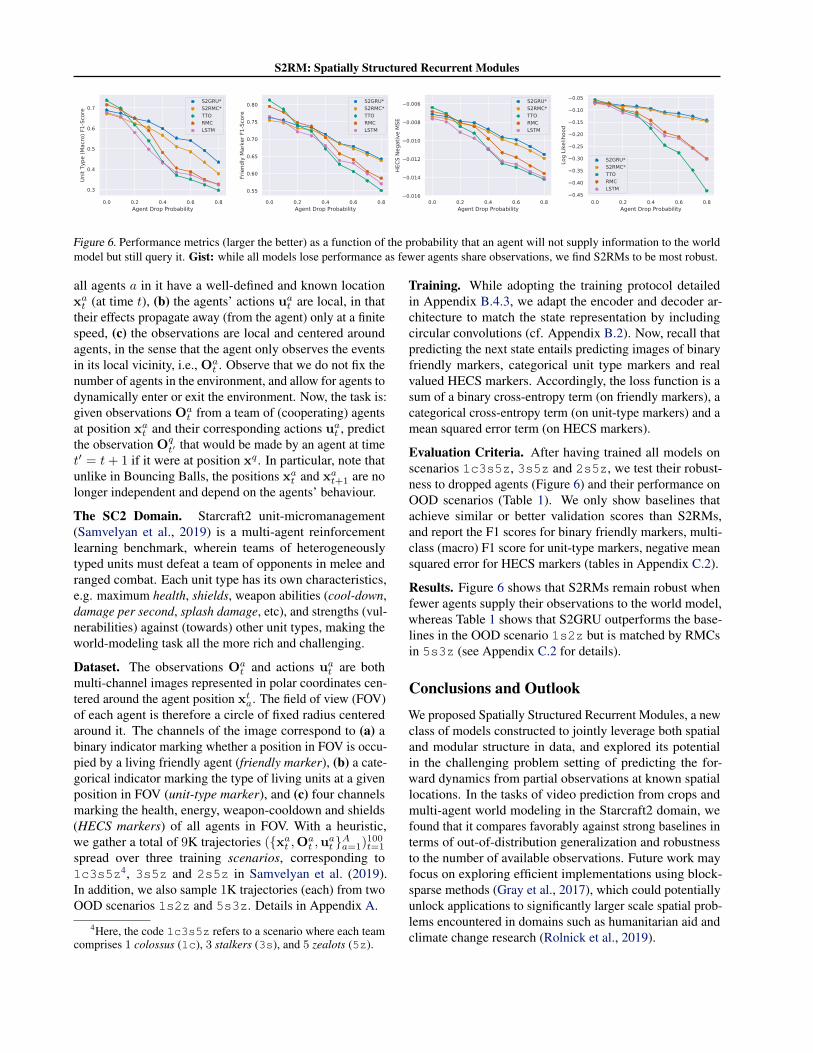
Figure 6. Performance metrics (larger the better) as a function of the probability that an agent will not supply information to the worldmodel but still query it. Gist: while all models lose performance as fewer agents share observations, we find S2RMs to be most robust.
all agents a in it have a well-defined and known locationxat (at time t), (b) the agents’ actions ua
t are local, in thattheir effects propagate away (from the agent) only at a finitespeed, (c) the observations are local and centered aroundagents, in the sense that the agent only observes the eventsin its local vicinity, i.e., Oa
t . Observe that we do not fix thenumber of agents in the environment, and allow for agents todynamically enter or exit the environment. Now, the task is:given observations Oa
t from a team of (cooperating) agentsat position xa
t and their corresponding actions uat , predict
the observation Oqt′ that would be made by an agent at time
t′ = t+ 1 if it were at position xq. In particular, note thatunlike in Bouncing Balls, the positions xa
t and xat+1 are no
longer independent and depend on the agents’ behaviour.
The SC2 Domain. Starcraft2 unit-micromanagement(Samvelyan et al., 2019) is a multi-agent reinforcementlearning benchmark, wherein teams of heterogeneouslytyped units must defeat a team of opponents in melee andranged combat. Each unit type has its own characteristics,e.g. maximum health, shields, weapon abilities (cool-down,damage per second, splash damage, etc), and strengths (vul-nerabilities) against (towards) other unit types, making theworld-modeling task all the more rich and challenging.
Dataset. The observations Oat and actions ua
t are bothmulti-channel images represented in polar coordinates cen-tered around the agent position xt
a. The field of view (FOV)of each agent is therefore a circle of fixed radius centeredaround it. The channels of the image correspond to (a) abinary indicator marking whether a position in FOV is occu-pied by a living friendly agent (friendly marker), (b) a cate-gorical indicator marking the type of living units at a givenposition in FOV (unit-type marker), and (c) four channelsmarking the health, energy, weapon-cooldown and shields(HECS markers) of all agents in FOV. With a heuristic,we gather a total of 9K trajectories ({xa
t ,Oat ,u
at }Aa=1)100t=1
spread over three training scenarios, corresponding to1c3s5z4, 3s5z and 2s5z in Samvelyan et al. (2019).In addition, we also sample 1K trajectories (each) from twoOOD scenarios 1s2z and 5s3z. Details in Appendix A.
4Here, the code 1c3s5z refers to a scenario where each teamcomprises 1 colossus (1c), 3 stalkers (3s), and 5 zealots (5z).
Training. While adopting the training protocol detailedin Appendix B.4.3, we adapt the encoder and decoder ar-chitecture to match the state representation by includingcircular convolutions (cf. Appendix B.2). Now, recall thatpredicting the next state entails predicting images of binaryfriendly markers, categorical unit type markers and realvalued HECS markers. Accordingly, the loss function is asum of a binary cross-entropy term (on friendly markers), acategorical cross-entropy term (on unit-type markers) and amean squared error term (on HECS markers).
Evaluation Criteria. After having trained all models onscenarios 1c3s5z, 3s5z and 2s5z, we test their robust-ness to dropped agents (Figure 6) and their performance onOOD scenarios (Table 1). We only show baselines thatachieve similar or better validation scores than S2RMs,and report the F1 scores for binary friendly markers, multi-class (macro) F1 score for unit-type markers, negative meansquared error for HECS markers (tables in Appendix C.2).
Results. Figure 6 shows that S2RMs remain robust whenfewer agents supply their observations to the world model,whereas Table 1 shows that S2GRU outperforms the base-lines in the OOD scenario 1s2z but is matched by RMCsin 5s3z (see Appendix C.2 for details).
Conclusions and OutlookWe proposed Spatially Structured Recurrent Modules, a newclass of models constructed to jointly leverage both spatialand modular structure in data, and explored its potentialin the challenging problem setting of predicting the for-ward dynamics from partial observations at known spatiallocations. In the tasks of video prediction from crops andmulti-agent world modeling in the Starcraft2 domain, wefound that it compares favorably against strong baselines interms of out-of-distribution generalization and robustnessto the number of available observations. Future work mayfocus on exploring efficient implementations using block-sparse methods (Gray et al., 2017), which could potentiallyunlock applications to significantly larger scale spatial prob-lems encountered in domains such as humanitarian aid andclimate change research (Rolnick et al., 2019).
S2RM: Spatially Structured Recurrent Modules
AcknowledgementsThe authors would like to thank Georgios Arvanitidis, LuigiGresele for their feedback on the paper, and Murray Shana-han for the discussions. The authors also acknowledge theimportant role played by their colleagues at the Empiri-cal Inference Department of MPI-IS Tubingen and Milathroughout the duration of this work.
ReferencesAlet, F., Lozano-Perez, T., and Kaelbling, L. P. Modular
meta-learning. arXiv preprint arXiv:1806.10166, 2018.
Battaglia, P. W., Hamrick, J. B., Bapst, V., Sanchez-Gonzalez, A., Zambaldi, V., Malinowski, M., Tacchetti,A., Raposo, D., Santoro, A., Faulkner, R., et al. Rela-tional inductive biases, deep learning, and graph networks.arXiv preprint arXiv:1806.01261, 2018.
Bengio, Y., Deleu, T., Rahaman, N., Ke, R., Lachapelle,S., Bilaniuk, O., Goyal, A., and Pal, C. A meta-transferobjective for learning to disentangle causal mechanisms.arXiv preprint arXiv:1901.10912, 2019.
Cho, K., Van Merrienboer, B., Gulcehre, C., Bahdanau,D., Bougares, F., Schwenk, H., and Bengio, Y. Learn-ing phrase representations using rnn encoder-decoderfor statistical machine translation. arXiv preprintarXiv:1406.1078, 2014.
Eslami, S. A., Rezende, D. J., Besse, F., Viola, F., Morcos,A. S., Garnelo, M., Ruderman, A., Rusu, A. A., Dani-helka, I., Gregor, K., et al. Neural scene representationand rendering. Science, 360(6394):1204–1210, 2018.
Fasshauer, G. E. Positive definite kernels: past, present andfuture. 2011.
Garnelo, M., Schwarz, J., Rosenbaum, D., Viola, F.,Rezende, D. J., Eslami, S., and Teh, Y. W. Neural pro-cesses. arXiv preprint arXiv:1807.01622, 2018.
Goyal, A., Lamb, A., Hoffmann, J., Sodhani, S., Levine,S., Bengio, Y., and Scholkopf, B. Recurrent independentmechanisms. arXiv preprint arXiv:1909.10893, 2019.
Graves, A., Wayne, G., and Danihelka, I. Neural turingmachines. arXiv preprint arXiv:1410.5401, 2014.
Graves, A., Wayne, G., Reynolds, M., Harley, T., Dani-helka, I., Grabska-Barwinska, A., Colmenarejo, S. G.,Grefenstette, E., Ramalho, T., Agapiou, J., et al. Hybridcomputing using a neural network with dynamic externalmemory. Nature, 538(7626):471–476, 2016.
Gray, S., Radford, A., and Kingma, D. P. Gpu kernels forblock-sparse weights. arXiv preprint arXiv:1711.09224,3, 2017.
Henaff, M., Weston, J., Szlam, A., Bordes, A., and LeCun,Y. Tracking the world state with recurrent entity networks,2016.
Hochreiter, S. and Schmidhuber, J. Long short-term memory.Neural computation, 9(8):1735–1780, 1997.
Jacobs, R. A., Jordan, M. I., Nowlan, S. J., and Hinton, G. E.Adaptive mixtures of local experts. Neural computation,3(1):79–87, 1991.
Jaderberg, M., Simonyan, K., Zisserman, A., andKavukcuoglu, K. Spatial transformer networks, 2015.
Ke, N. R., GOYAL, A. G. A. P., Bilaniuk, O., Binas, J.,Mozer, M. C., Pal, C., and Bengio, Y. Sparse attentivebacktracking: Temporal credit assignment through re-minding. In Advances in neural information processingsystems, pp. 7640–7651, 2018.
Ke, N. R., Bilaniuk, O., Goyal, A., Bauer, S., Larochelle,H., Pal, C., and Bengio, Y. Learning neural causalmodels from unknown interventions. arXiv preprintarXiv:1910.01075, 2019.
Kingma, D. P. and Ba, J. Adam: A method for stochasticoptimization. arXiv preprint arXiv:1412.6980, 2014.
Kumar, A., Eslami, S., Rezende, D. J., Garnelo, M., Viola,F., Lockhart, E., and Shanahan, M. Consistent generativequery networks. arXiv preprint arXiv:1807.02033, 2018.
Li, S., Li, W., Cook, C., Zhu, C., and Gao, Y. Indepen-dently recurrent neural network (indrnn): Building alonger and deeper rnn. In Proceedings of the IEEE Con-ference on Computer Vision and Pattern Recognition, pp.5457–5466, 2018.
Miladinovic, D., Gondal, M. W., Scholkopf, B., Buhmann,J. M., and Bauer, S. Disentangled state space representa-tions. arXiv preprint arXiv:1906.03255, 2019.
Parascandolo, G., Kilbertus, N., Rojas-Carulla, M., andScholkopf, B. Learning independent causal mechanisms.arXiv preprint arXiv:1712.00961, 2017.
Parmar, N., Vaswani, A., Uszkoreit, J., ukasz Kaiser,Shazeer, N., Ku, A., and Tran, D. Image transformer,2018.
Paszke, A., Gross, S., Massa, F., Lerer, A., Bradbury, J.,Chanan, G., Killeen, T., Lin, Z., Gimelshein, N., Antiga,L., Desmaison, A., Kopf, A., Yang, E., DeVito, Z., Rai-son, M., Tejani, A., Chilamkurthy, S., Steiner, B., Fang,L., Bai, J., and Chintala, S. Pytorch: An imperativestyle, high-performance deep learning library. In Wal-lach, H., Larochelle, H., Beygelzimer, A., d’ Alche-Buc,F., Fox, E., and Garnett, R. (eds.), Advances in Neural In-formation Processing Systems 32, pp. 8024–8035. CurranAssociates, Inc., 2019.
S2RM: Spatially Structured Recurrent Modules
Rolnick, D., Donti, P. L., Kaack, L. H., Kochanski, K.,Lacoste, A., Sankaran, K., Ross, A. S., Milojevic-Dupont,N., Jaques, N., Waldman-Brown, A., et al. Tacklingclimate change with machine learning. arXiv preprintarXiv:1906.05433, 2019.
Samvelyan, M., Rashid, T., de Witt, C. S., Farquhar, G.,Nardelli, N., Rudner, T. G. J., Hung, C.-M., Torr, P. H. S.,Foerster, J., and Whiteson, S. The starcraft multi-agentchallenge, 2019.
Santoro, A., Raposo, D., Barrett, D. G., Malinowski, M.,Pascanu, R., Battaglia, P., and Lillicrap, T. A simple neu-ral network module for relational reasoning. In Advancesin neural information processing systems, pp. 4967–4976,2017.
Santoro, A., Faulkner, R., Raposo, D., Rae, J., Chrzanowski,M., Weber, T., Wierstra, D., Vinyals, O., Pascanu, R., andLillicrap, T. Relational recurrent neural networks. InAdvances in Neural Information Processing Systems, pp.7299–7310, 2018.
Shazeer, N., Mirhoseini, A., Maziarz, K., Davis, A., Le,Q., Hinton, G., and Dean, J. Outrageously large neuralnetworks: The sparsely-gated mixture-of-experts layer.arXiv preprint arXiv:1701.06538, 2017.
Singh, G., Yoon, J., Son, Y., and Ahn, S. Sequential neuralprocesses, 2019.
Sun, C., Karlsson, P., Wu, J., Tenenbaum, J. B., and Mur-phy, K. Predicting the present and future states of multi-agent systems from partially-observed visual data. InInternational Conference on Learning Representations,2019. URL https://openreview.net/forum?id=r1xdH3CcKX.
Vaswani, A., Shazeer, N., Parmar, N., Uszkoreit, J., Jones,L., Gomez, A. N., Kaiser, Ł., and Polosukhin, I. Atten-tion is all you need. In Advances in neural informationprocessing systems, pp. 5998–6008, 2017.
Velickovic, P., Cucurull, G., Casanova, A., Romero, A.,Lio, P., and Bengio, Y. Graph attention networks. arXivpreprint arXiv:1710.10903, 2017.
Vinyals, O., Ewalds, T., Bartunov, S., Georgiev, P., Vezhn-evets, A. S., Yeo, M., Makhzani, A., Kuttler, H., Agapiou,J., Schrittwieser, J., et al. Starcraft ii: A new challenge forreinforcement learning. arXiv preprint arXiv:1708.04782,2017.
Wang, X., Girshick, R., Gupta, A., and He, K. Non-localneural networks, 2017.
Zhang, H., Goodfellow, I., Metaxas, D., and Odena, A. Self-attention generative adversarial networks. arXiv preprintarXiv:1805.08318, 2018.
S2RM: Spatially Structured Recurrent Modules
A. Starcraft2The Starcraft2 Environment we use is a modified versionof the SMAC-Env proposed in Samvelyan et al. (2019) andbuilt on PySC2 wrapper around Blizzard SC2 API (Vinyalset al., 2017). Starcraft2 is a real-time-strategy (RTS) gamewhere players are tasked with manufacturing and controllingarmies of units (airborne or land-based) to defeat the oppo-nent’s army (where the opponent can be an AI or anotherhuman). The players must choose their alien race5 beforestarting the game; available options are Protoss, Terranand Zerg. All unit types (of all races) have their strengthsand weaknesses against other unit types, be it in terms ofmaximum health, shields (Protoss), energy (Terran), DPS(damage per second, related to weapon cooldown), splashdamage, or manufacturing costs (measured in minerals andvespene gas, which must be mined).
The key engineering contribution of Samvelyan et al. (2019)is to repurpose the RTS game as a multi-agent environment,where the individual units in the army become individualagents6. The result is a rich and challenging environmentwhere heterogeneous teams of agents must defeat each otherin melee and ranged combat. The composition of teamsvary between scenarios, of which Samvelyan et al. (2019)provide a selection. Further, new scenarios can be easilycreated with the SC2MapEditor, which allows for practicallyendlessly many possibilities.
We build on Samvelyan et al. (2019) by modifying their envi-ronment to better expose the transfer and out-of-distributionaspects of the domain by (a) standardizing the state andaction space across a large class of scenarios and (b) stan-dardizing the unit stats to better reflect the game-definednotion of hit-points.
A.1. Standardized State Space for All Scenarios
In the environment provided by Samvelyan et al. (2019),the dimensionality of the vector state space varies with thenumber of friendly and enemy agents, which in turn varieswith the scenario. While this is not an issue in the typicaluse case of training MARL agents in a fixed scenario, it isnot convenient for designing models that seamlessly handlemultiple scenarios. In the following, we propose an alternatestate representation that preserves the spatial structure andis consistent across multiple scenarios.
Instead of representing the state of an agent a with a vectorof variable dimension, we represent it with a multi-channelpolar image Ia of shape C × I × J , where C is the numberof channels and (I, J) is the image size. Given the radial
5Please note that this is a game-specific notion.6Note that this is rather unconventional, since each player usu-
ally controls entire armies and must switch between macro- andmicro-management of units or unit-groups.
and angular resolutions ρ and ϕ (respectively), the pixelcoordinate i = 0, ..., I − 1, j = 0, ..., J − 1 corresponds tocoordinates (i · ρ, j · ϕ) with respect to a polar coordinatesystem centered on the agent a, where the positive x-axis(j = 0) points towards the east. Further, the field of view(FOV) of an agent is characterized by a circle of radiusI · ρ centered on the agent at 2D game-coordinates xa =(xa1 , x
a2), to which the Starcraft2 API (Vinyals et al., 2017)
provides raw access.
The polar image Ia therefore provides an agent-centric viewof the environment, where pixel coordinates i, j in Ia canbe mapped to global game coordinates x = (x1, x2) in FOVvia:
x1 = i · ρ cos [j · ϕ] + xa1 (21)x2 = i · ρ sin [j · ϕ] + xa2 (22)
In what follows, we denote this transformation with Ta, asin Ta(i, j) = (x1, x2).
Now, the channels in the polar image can encode variousaspects of the observation; in our case: friendly markers(one channel), unit-type markers (nine channels, one-hot),health-energy-cooldown-shields (HECS, four channels) andterrain height (one channel). As an example, let us considerthe friendly markers, which is a binary indicator markingunits that are friendly. If we have an agent at game position(x1, x2) that is friendly to agent a, then we would expect thepixel coordinate (i, j) = T−1a (x1, x2) of the correspondingchannel in the polar image Ia to be 1, but 0 otherwise. Like-wise, the value of I at the channels corresponding to HECSat pixel position i, j gives the HECS of the correspondingunit7 at Ta(i, j). This representation has the following ad-vantages: (a) it does not depend on the number of units inthe field of view, (b) it exposes the spatial structure in thearrangement of units which can naturally processed by con-volutional neural networks (e.g. with circular convolutions).
Nevertheless, it has the disadvantage that the positions arequantized to pixels, but the euclidean distance between thelocations represented by pixels (i, j) and (i, j+1) increaseswith increasing i. Consequently, this representation may notremain suitable for larger FOVs.
Further, this representation is also appropriate for the actionspace. Given an agent, we represent the one-hot categoricalactions of all friendly agents in FOV as a multi-channel polarimage. In this representation, the pixel position i, j gives theaction taken by an agent at at position Ta(i, j). Unfriendlyagents get assigned an ”unknown action”, whereas positionsnot occupied by a living agent are assigned a ”no-op” action.
7If health drops to zero, the unit is considered dead and therepresentation does not differentiate between dead and absent units.

S2RM: Spatially Structured Recurrent Modules
(a) 1s2z (1 Stalker and 2 Zealots per team). (b) 5s3z (5 Stalkers and 3 Zealots per team).
(c) 2s3z (2 Stalkers and 3 Zealots per team). (d) 3s5z (3 Stalkers and 5 Zealots per team).
(e) 1c3s5z (1 Colossus, 3 Stalkers and 5 Zealots per team).
Figure 7. Human readable illustrations of the Starcraft2 (SMAC) scenarios we consider in this work. Figures 7a and 7b show the OODscenarios, whereas Figures 7c, 7d and 7e show the training scenarios (provided by Samvelyan et al. (2019)).
A.2. Standardized Unit Stats
At any given point in time, an active unit in Starcraft2 hascertain stats, e.g. its health, energy (Terran), shields (Pro-toss) and weapon-cooldown (for armed units). A large andexpensive unit-type like the Colossus has more max-health(hit-points) than smaller units like Stalkers and Marines8.Likewise, unit-types differ in the rate at which they dealdamage (measured in damage-per-second or DPS, exclud-ing splash damage), which in turn depends on the cooldownduration of the active weapon.
Now, the environment provided by Samvelyan et al. (2019)normalizes the stats by their respective maximum value,resulting in values between 0 and 1. However, given thatdifferent units may have different normalization, the statsare rendered incomparable between unit types (without addi-tionally accounting the unit-type). We address this by stan-
8These stats may change with game-versions, and are cata-logued here: https://liquipedia.net/starcraft2/Units_(StarCraft).
dardizing stats (instead of normalizing) by dividing themby a fixed value. In this scheme, the stats are scaled uni-formly across all unit-types, enabling models to directlyrely on them instead of having to account for the respectiveunit-types.
B. Hyperparameters and ArchitecturesB.1. Encoder and Decoder for Bouncing Balls
The architectures of image encoder and decoder was fixedfor all models after initial experimentation. We convergedto the following architectures.
B.1.1. S2RMS
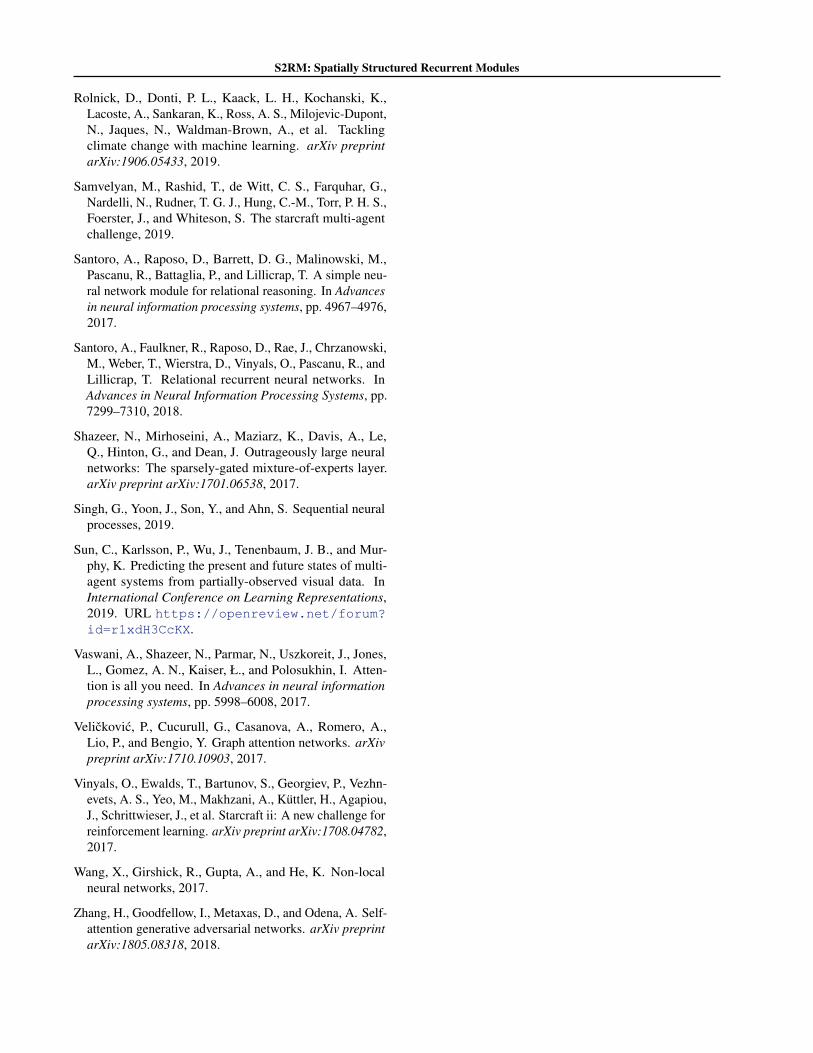
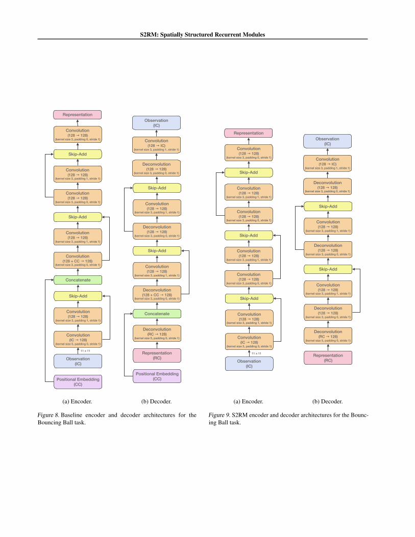
The encoder (decoder) is a (de)convolutional network withresidual connections (Figure 9).
S2RM: Spatially Structured Recurrent Modules
Convolution (IC → 128)
(kernel size 5, padding 0, stride 1)
Convolution (128 → 128)
(kernel size 3, padding 1, stride 1)
Convolution (128 + CC → 128)
(kernel size 3, padding 0, stride 1)
Concatenate
Convolution (128 → 128)
(kernel size 3, padding 1, stride 1)
Convolution (128 → 128)
(kernel size 3, padding 0, stride 1)
Convolution (128 → 128)
(kernel size 3, padding 1, stride 1)
Convolution (128 → 128)
(kernel size 3, padding 0, stride 1)
Observation (IC)
Representation
Skip-Add
Skip-Add
Positional Embedding (CC)
Skip-Add
11 x 11
(a) Encoder.
Deconvolution (RC → 128)
(kernel size 5, padding 0, stride 1)
Representation (RC)
Positional Embedding (CC)
Concatenate
Deconvolution (128 + CC → 128)
(kernel size 3, padding 0, stride 1)
Convolution (128 → 128)
(kernel size 3, padding 1, stride 1)
Skip-Add
Deconvolution (128 → 128)
(kernel size 3, padding 0, stride 1)
Convolution (128 → 128)
(kernel size 3, padding 1, stride 1)
Skip-Add
Deconvolution (128 → 128)
(kernel size 3, padding 0, stride 1)
Convolution (128 → IC)
(kernel size 3, padding 1, stride 1)
Observation (IC)
(b) Decoder.
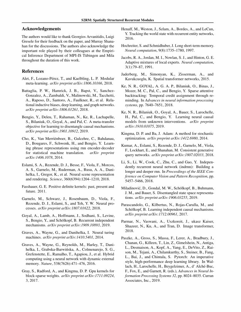
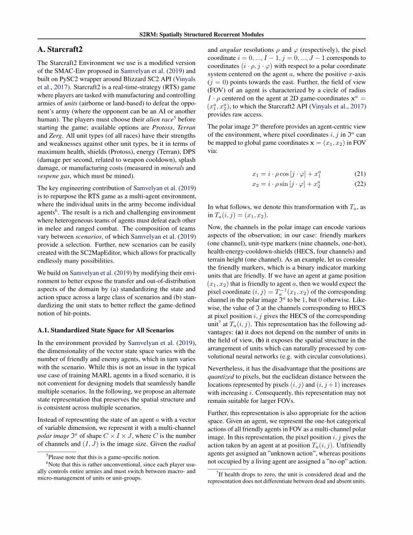
Figure 8. Baseline encoder and decoder architectures for theBouncing Ball task.
Convolution (IC → 128)
(kernel size 5, padding 0, stride 1)
Convolution (128 → 128)
(kernel size 3, padding 1, stride 1)
Convolution (128 → 128)
(kernel size 3, padding 0, stride 1)
Convolution (128 → 128)
(kernel size 3, padding 1, stride 1)
Convolution (128 → 128)
(kernel size 3, padding 0, stride 1)
Convolution (128 → 128)
(kernel size 3, padding 1, stride 1)
Convolution (128 → 128)
(kernel size 3, padding 0, stride 1)
Observation (IC)
Representation
Skip-Add
Skip-Add
Skip-Add
11 x 11
(a) Encoder.
Deconvolution (RC → 128)
(kernel size 5, padding 0, stride 1)
Representation (RC)
Deconvolution (128 → 128)
(kernel size 3, padding 0, stride 1)
Convolution (128 → 128)
(kernel size 3, padding 1, stride 1)
Skip-Add
Deconvolution (128 → 128)
(kernel size 3, padding 0, stride 1)
Convolution (128 → 128)
(kernel size 3, padding 1, stride 1)
Skip-Add
Deconvolution (128 → 128)
(kernel size 3, padding 0, stride 1)
Convolution (128 → IC)
(kernel size 3, padding 1, stride 1)
Observation (IC)
(b) Decoder.
Figure 9. S2RM encoder and decoder architectures for the Bounc-ing Ball task.
S2RM: Spatially Structured Recurrent Modules
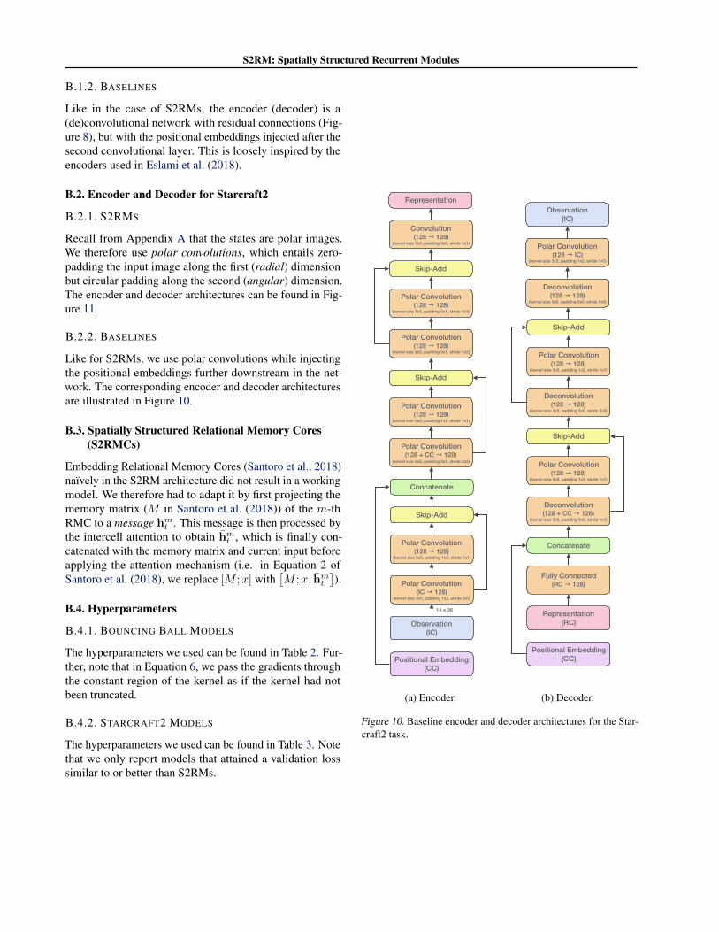
B.1.2. BASELINES
Like in the case of S2RMs, the encoder (decoder) is a(de)convolutional network with residual connections (Fig-ure 8), but with the positional embeddings injected after thesecond convolutional layer. This is loosely inspired by theencoders used in Eslami et al. (2018).
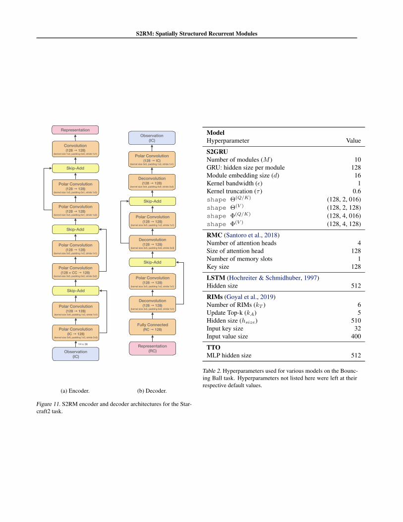
B.2. Encoder and Decoder for Starcraft2
B.2.1. S2RMS
Recall from Appendix A that the states are polar images.We therefore use polar convolutions, which entails zero-padding the input image along the first (radial) dimensionbut circular padding along the second (angular) dimension.The encoder and decoder architectures can be found in Fig-ure 11.
B.2.2. BASELINES
Like for S2RMs, we use polar convolutions while injectingthe positional embeddings further downstream in the net-work. The corresponding encoder and decoder architecturesare illustrated in Figure 10.
B.3. Spatially Structured Relational Memory Cores(S2RMCs)
Embedding Relational Memory Cores (Santoro et al., 2018)naıvely in the S2RM architecture did not result in a workingmodel. We therefore had to adapt it by first projecting thememory matrix (M in Santoro et al. (2018)) of the m-thRMC to a message hm
t . This message is then processed bythe intercell attention to obtain hm
t , which is finally con-catenated with the memory matrix and current input beforeapplying the attention mechanism (i.e. in Equation 2 ofSantoro et al. (2018), we replace [M ;x] with
[M ;x, hm
t
]).
B.4. Hyperparameters
B.4.1. BOUNCING BALL MODELS
The hyperparameters we used can be found in Table 2. Fur-ther, note that in Equation 6, we pass the gradients throughthe constant region of the kernel as if the kernel had notbeen truncated.
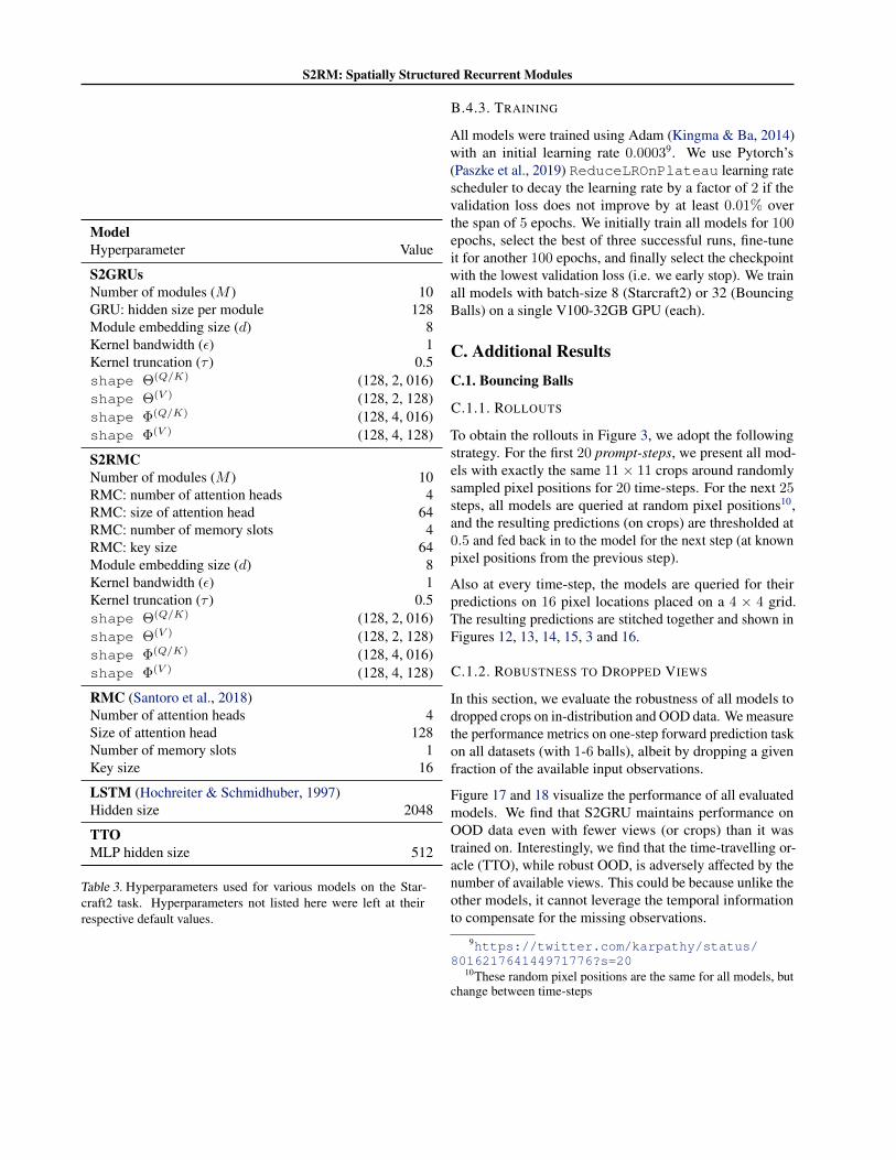
B.4.2. STARCRAFT2 MODELS
The hyperparameters we used can be found in Table 3. Notethat we only report models that attained a validation losssimilar to or better than S2RMs.
Polar Convolution (IC → 128)
(kernel size 3x5, padding 1x2, stride 2x3)
Polar Convolution (128 → 128)
(kernel size 3x5, padding 1x2, stride 1x1)
Polar Convolution (128 + CC → 128)
(kernel size 3x5, padding 0x2, stride 2x2)
Concatenate
Polar Convolution (128 → 128)
(kernel size 3x5, padding 1x2, stride 1x1)
Polar Convolution (128 → 128)
(kernel size 3x3, padding 0x1, stride 1x2)
Polar Convolution (128 → 128)
(kernel size 1x3, padding 0x1, stride 1x1)
Convolution (128 → 128)
(kernel size 1x3, padding 0x0, stride 1x1)
Observation (IC)
Representation
Skip-Add
Skip-Add
Positional Embedding (CC)
Skip-Add
14 x 36
(a) Encoder.
Deconvolution (128 + CC → 128)
(kernel size 3x5, padding 0x0, stride 1x1)
Polar Convolution (128 → 128)
(kernel size 3x5, padding 1x2, stride 1x1)
Skip-Add
Deconvolution (128 → 128)
(kernel size 3x5, padding 0x0, stride 2x3)
Polar Convolution (128 → 128)
(kernel size 3x5, padding 1x2, stride 1x1)
Skip-Add
Deconvolution (128 → 128)
(kernel size 3x5, padding 0x0, stride 2x2)
Polar Convolution (128 → IC)
(kernel size 3x5, padding 1x2, stride 1x1)
Observation (IC)
Fully Connected (RC → 128)
Representation (RC)
Positional Embedding (CC)
Concatenate
(b) Decoder.
Figure 10. Baseline encoder and decoder architectures for the Star-craft2 task.
S2RM: Spatially Structured Recurrent Modules
Polar Convolution (IC → 128)
(kernel size 3x5, padding 1x2, stride 2x3)
Polar Convolution (128 → 128)
(kernel size 3x5, padding 1x2, stride 1x1)
Polar Convolution (128 + CC → 128)
(kernel size 3x5, padding 0x2, stride 2x2)
Polar Convolution (128 → 128)
(kernel size 3x5, padding 1x2, stride 1x1)
Polar Convolution (128 → 128)
(kernel size 3x3, padding 0x1, stride 1x2)
Polar Convolution (128 → 128)
(kernel size 1x3, padding 0x1, stride 1x3)
Convolution (128 → 128)
(kernel size 1x3, padding 0x0, stride 1x1)
Observation (IC)
Representation
Skip-Add
Skip-Add
Skip-Add
14 x 36
(a) Encoder.
Fully Connected (RC → 128)
Representation (RC)
Deconvolution (128 → 128)
(kernel size 3x5, padding 0x0, stride 1x1)
Polar Convolution (128 → 128)
(kernel size 3x5, padding 1x2, stride 1x1)
Skip-Add
Deconvolution (128 → 128)
(kernel size 3x5, padding 0x0, stride 2x3)
Polar Convolution (128 → 128)
(kernel size 3x5, padding 1x2, stride 1x1)
Skip-Add
Deconvolution (128 → 128)
(kernel size 3x5, padding 0x0, stride 2x2)
Polar Convolution (128 → IC)
(kernel size 3x5, padding 1x2, stride 1x1)
Observation (IC)
(b) Decoder.
Figure 11. S2RM encoder and decoder architectures for the Star-craft2 task.
ModelHyperparameter Value
S2GRUNumber of modules (M ) 10GRU: hidden size per module 128Module embedding size (d) 16Kernel bandwidth (ε) 1Kernel truncation (τ ) 0.6shape Θ(Q/K) (128, 2, 016)shape Θ(V ) (128, 2, 128)shape Φ(Q/K) (128, 4, 016)shape Φ(V ) (128, 4, 128)
RMC (Santoro et al., 2018)Number of attention heads 4Size of attention head 128Number of memory slots 1Key size 128
LSTM (Hochreiter & Schmidhuber, 1997)Hidden size 512
RIMs (Goyal et al., 2019)Number of RIMs (kT ) 6Update Top-k (kA) 5Hidden size (hsize) 510Input key size 32Input value size 400
TTOMLP hidden size 512
Table 2. Hyperparameters used for various models on the Bounc-ing Ball task. Hyperparameters not listed here were left at theirrespective default values.
S2RM: Spatially Structured Recurrent Modules
ModelHyperparameter Value
S2GRUsNumber of modules (M ) 10GRU: hidden size per module 128Module embedding size (d) 8Kernel bandwidth (ε) 1Kernel truncation (τ ) 0.5shape Θ(Q/K) (128, 2, 016)shape Θ(V ) (128, 2, 128)shape Φ(Q/K) (128, 4, 016)shape Φ(V ) (128, 4, 128)
S2RMCNumber of modules (M ) 10RMC: number of attention heads 4RMC: size of attention head 64RMC: number of memory slots 4RMC: key size 64Module embedding size (d) 8Kernel bandwidth (ε) 1Kernel truncation (τ ) 0.5shape Θ(Q/K) (128, 2, 016)shape Θ(V ) (128, 2, 128)shape Φ(Q/K) (128, 4, 016)shape Φ(V ) (128, 4, 128)
RMC (Santoro et al., 2018)Number of attention heads 4Size of attention head 128Number of memory slots 1Key size 16
LSTM (Hochreiter & Schmidhuber, 1997)Hidden size 2048
TTOMLP hidden size 512
Table 3. Hyperparameters used for various models on the Star-craft2 task. Hyperparameters not listed here were left at theirrespective default values.
B.4.3. TRAINING
All models were trained using Adam (Kingma & Ba, 2014)with an initial learning rate 0.00039. We use Pytorch’s(Paszke et al., 2019) ReduceLROnPlateau learning ratescheduler to decay the learning rate by a factor of 2 if thevalidation loss does not improve by at least 0.01% overthe span of 5 epochs. We initially train all models for 100epochs, select the best of three successful runs, fine-tuneit for another 100 epochs, and finally select the checkpointwith the lowest validation loss (i.e. we early stop). We trainall models with batch-size 8 (Starcraft2) or 32 (BouncingBalls) on a single V100-32GB GPU (each).
C. Additional ResultsC.1. Bouncing Balls
C.1.1. ROLLOUTS
To obtain the rollouts in Figure 3, we adopt the followingstrategy. For the first 20 prompt-steps, we present all mod-els with exactly the same 11× 11 crops around randomlysampled pixel positions for 20 time-steps. For the next 25steps, all models are queried at random pixel positions10,and the resulting predictions (on crops) are thresholded at0.5 and fed back in to the model for the next step (at knownpixel positions from the previous step).
Also at every time-step, the models are queried for theirpredictions on 16 pixel locations placed on a 4 × 4 grid.The resulting predictions are stitched together and shown inFigures 12, 13, 14, 15, 3 and 16.
C.1.2. ROBUSTNESS TO DROPPED VIEWS
In this section, we evaluate the robustness of all models todropped crops on in-distribution and OOD data. We measurethe performance metrics on one-step forward prediction taskon all datasets (with 1-6 balls), albeit by dropping a givenfraction of the available input observations.
Figure 17 and 18 visualize the performance of all evaluatedmodels. We find that S2GRU maintains performance onOOD data even with fewer views (or crops) than it wastrained on. Interestingly, we find that the time-travelling or-acle (TTO), while robust OOD, is adversely affected by thenumber of available views. This could be because unlike theother models, it cannot leverage the temporal informationto compensate for the missing observations.
9https://twitter.com/karpathy/status/801621764144971776?s=20
10These random pixel positions are the same for all models, butchange between time-steps
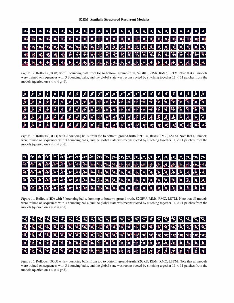
S2RM: Spatially Structured Recurrent Modules
Figure 12. Rollouts (OOD) with 1 bouncing ball, from top to bottom: ground-truth, S2GRU, RIMs, RMC, LSTM. Note that all modelswere trained on sequences with 3 bouncing balls, and the global state was reconstructed by stitching together 11× 11 patches from themodels (queried on a 4× 4 grid).
Figure 13. Rollouts (OOD) with 2 bouncing balls, from top to bottom: ground-truth, S2GRU, RIMs, RMC, LSTM. Note that all modelswere trained on sequences with 3 bouncing balls, and the global state was reconstructed by stitching together 11× 11 patches from themodels (queried on a 4× 4 grid).
Figure 14. Rollouts (ID) with 3 bouncing balls, from top to bottom: ground-truth, S2GRU, RIMs, RMC, LSTM. Note that all modelswere trained on sequences with 3 bouncing balls, and the global state was reconstructed by stitching together 11× 11 patches from themodels (queried on a 4× 4 grid).
Figure 15. Rollouts (OOD) with 4 bouncing balls, from top to bottom: ground-truth, S2GRU, RIMs, RMC, LSTM. Note that all modelswere trained on sequences with 3 bouncing balls, and the global state was reconstructed by stitching together 11× 11 patches from themodels (queried on a 4× 4 grid).

S2RM: Spatially Structured Recurrent Modules
Figure 16. Rollouts (OOD) with 6 bouncing balls, from top to bottom: ground-truth, S2GRU, RIMs, RMC, LSTM. Note that all modelswere trained on sequences with 3 bouncing balls, and the global state was reconstructed by stitching together 11× 11 patches from themodels (queried on a 4× 4 grid).
C.2. Starcraft2
C.2.1. TABULAR RESULTS
The results used to plot Figure 6 can be found tabulated inTables 4, 5, 6 and 7.

S2RM: Spatially Structured Recurrent Modules
0.2 0.3 0.4 0.5 0.6 0.7 0.8 0.9 1.0Fraction of Available Views
12
34
56
Num
ber o
f Bou
ncin
g Ba
lls
0.949 0.961 0.968 0.971 0.974 0.975 0.976 0.977 0.978
0.933 0.959 0.969 0.974 0.977 0.979 0.980 0.981 0.982
0.915 0.946 0.960 0.967 0.971 0.974 0.975 0.977 0.978
0.869 0.907 0.927 0.939 0.946 0.950 0.954 0.956 0.958
0.823 0.856 0.879 0.893 0.902 0.909 0.915 0.918 0.921
0.785 0.812 0.832 0.845 0.856 0.863 0.869 0.873 0.877 0.72
0.78
0.84
0.90
0.96
(a) S2GRU
0.2 0.3 0.4 0.5 0.6 0.7 0.8 0.9 1.0Fraction of Available Views
12
34
56
Num
ber o
f Bou
ncin
g Ba
lls
0.933 0.948 0.954 0.958 0.960 0.962 0.963 0.964 0.964
0.926 0.950 0.962 0.968 0.972 0.974 0.976 0.977 0.977
0.916 0.950 0.964 0.971 0.975 0.977 0.979 0.980 0.981
0.866 0.900 0.918 0.930 0.937 0.941 0.945 0.947 0.949
0.819 0.844 0.859 0.869 0.877 0.882 0.886 0.889 0.891
0.781 0.797 0.808 0.815 0.821 0.825 0.828 0.830 0.832 0.72
0.78
0.84
0.90
0.96
(b) RIMs
0.2 0.3 0.4 0.5 0.6 0.7 0.8 0.9 1.0Fraction of Available Views
12
34
56
Num
ber o
f Bou
ncin
g Ba
lls
0.917 0.929 0.936 0.941 0.944 0.947 0.948 0.949 0.950
0.897 0.923 0.937 0.945 0.950 0.953 0.956 0.958 0.959
0.885 0.935 0.957 0.966 0.971 0.974 0.976 0.977 0.978
0.814 0.835 0.850 0.859 0.866 0.871 0.875 0.878 0.881
0.770 0.783 0.792 0.799 0.804 0.807 0.810 0.812 0.814
0.738 0.746 0.751 0.755 0.759 0.761 0.762 0.763 0.764 0.72
0.78
0.84
0.90
0.96
(c) RMC
0.2 0.3 0.4 0.5 0.6 0.7 0.8 0.9 1.0Fraction of Available Views
12
34
56
Num
ber o
f Bou
ncin
g Ba
lls0.916 0.928 0.935 0.940 0.942 0.943 0.943 0.942 0.941
0.896 0.920 0.934 0.943 0.949 0.952 0.955 0.958 0.960
0.893 0.931 0.948 0.957 0.962 0.965 0.967 0.969 0.970
0.825 0.843 0.854 0.861 0.867 0.871 0.874 0.876 0.878
0.780 0.791 0.798 0.803 0.806 0.808 0.811 0.812 0.814
0.747 0.753 0.758 0.761 0.763 0.764 0.765 0.766 0.766 0.72
0.78
0.84
0.90
0.96
(d) LSTM
0.2 0.3 0.4 0.5 0.6 0.7 0.8 0.9 1.0Fraction of Available Views
12
34
56
Num
ber o
f Bou
ncin
g Ba
lls
0.909 0.929 0.949 0.965 0.977 0.986 0.993 0.997 1.000
0.850 0.880 0.913 0.939 0.960 0.975 0.987 0.995 0.999
0.808 0.846 0.885 0.918 0.944 0.964 0.980 0.992 0.998
0.776 0.817 0.861 0.898 0.927 0.951 0.971 0.986 0.994
0.750 0.793 0.838 0.877 0.909 0.936 0.958 0.975 0.984
0.729 0.771 0.816 0.856 0.889 0.917 0.941 0.957 0.967 0.72
0.78
0.84
0.90
0.96
(e) TTO
Figure 17. Balanced accuracy (arithmetic mean of recall and specificity) achieved by all evaluated models for one-step forward predictiontask with various number of balls and fractions of available views. All models were trained on video sequences with 3 balls and a constantnumber of crops / views (10 views, corresponding to the right-most columns labelled 1.0). The color map is consistent across all plots.
S2RM: Spatially Structured Recurrent Modules
0.2 0.3 0.4 0.5 0.6 0.7 0.8 0.9 1.0Fraction of Available Views
12
34
56
Num
ber o
f Bou
ncin
g Ba
lls
0.894 0.914 0.924 0.929 0.934 0.935 0.938 0.939 0.940
0.894 0.933 0.948 0.956 0.961 0.964 0.965 0.967 0.968
0.877 0.921 0.941 0.951 0.957 0.960 0.963 0.964 0.966
0.820 0.871 0.898 0.914 0.924 0.930 0.935 0.938 0.941
0.763 0.808 0.838 0.858 0.870 0.879 0.886 0.891 0.895
0.718 0.756 0.782 0.800 0.814 0.824 0.832 0.837 0.842 0.64
0.72
0.80
0.88
0.96
(a) S2GRU
0.2 0.3 0.4 0.5 0.6 0.7 0.8 0.9 1.0Fraction of Available Views
12
34
56
Num
ber o
f Bou
ncin
g Ba
lls
0.836 0.862 0.874 0.882 0.886 0.889 0.891 0.893 0.894
0.878 0.917 0.937 0.947 0.953 0.957 0.960 0.962 0.963
0.880 0.928 0.948 0.958 0.963 0.966 0.968 0.970 0.971
0.821 0.866 0.891 0.906 0.915 0.921 0.926 0.929 0.931
0.764 0.798 0.819 0.833 0.843 0.850 0.855 0.860 0.863
0.714 0.738 0.754 0.765 0.773 0.778 0.783 0.786 0.789 0.64
0.72
0.80
0.88
0.96
(b) RIMs
0.2 0.3 0.4 0.5 0.6 0.7 0.8 0.9 1.0Fraction of Available Views
12
34
56
Num
ber o
f Bou
ncin
g Ba
lls
0.808 0.826 0.836 0.842 0.847 0.849 0.851 0.852 0.852
0.822 0.859 0.880 0.892 0.899 0.904 0.907 0.911 0.913
0.832 0.905 0.937 0.950 0.957 0.962 0.964 0.966 0.967
0.744 0.777 0.799 0.813 0.823 0.831 0.837 0.841 0.845
0.690 0.711 0.725 0.735 0.742 0.748 0.753 0.756 0.759
0.646 0.659 0.668 0.674 0.680 0.683 0.686 0.687 0.689 0.64
0.72
0.80
0.88
0.96
(c) RMC
0.2 0.3 0.4 0.5 0.6 0.7 0.8 0.9 1.0Fraction of Available Views
12
34
56
Num
ber o
f Bou
ncin
g Ba
lls0.806 0.823 0.833 0.838 0.840 0.837 0.832 0.824 0.820
0.821 0.858 0.880 0.894 0.903 0.910 0.915 0.919 0.922
0.842 0.898 0.924 0.937 0.944 0.949 0.952 0.953 0.955
0.762 0.790 0.807 0.817 0.825 0.831 0.835 0.839 0.841
0.706 0.723 0.734 0.742 0.747 0.751 0.755 0.757 0.759
0.661 0.672 0.678 0.683 0.686 0.689 0.691 0.692 0.693 0.64
0.72
0.80
0.88
0.96
(d) LSTM
0.2 0.3 0.4 0.5 0.6 0.7 0.8 0.9 1.0Fraction of Available Views
12
34
56
Num
ber o
f Bou
ncin
g Ba
lls
0.895 0.918 0.942 0.959 0.972 0.983 0.991 0.997 1.000
0.819 0.859 0.900 0.929 0.951 0.969 0.984 0.994 0.999
0.759 0.814 0.865 0.903 0.933 0.956 0.976 0.990 0.997
0.710 0.773 0.834 0.879 0.914 0.942 0.966 0.983 0.991
0.667 0.736 0.803 0.854 0.893 0.925 0.951 0.970 0.979
0.630 0.702 0.772 0.827 0.869 0.904 0.931 0.949 0.958 0.64
0.72
0.80
0.88
0.96
(e) TTO
Figure 18. F1-Score (harmonic mean of precision and recall) achieved by all evaluated models for one-step forward prediction task withvarious number of balls and fractions of available views. All models were trained on video sequences with 3 balls and a constant numberof crops / views (10 views, corresponding to the right-most columns labelled 1.0). The color map is consistent across all plots.
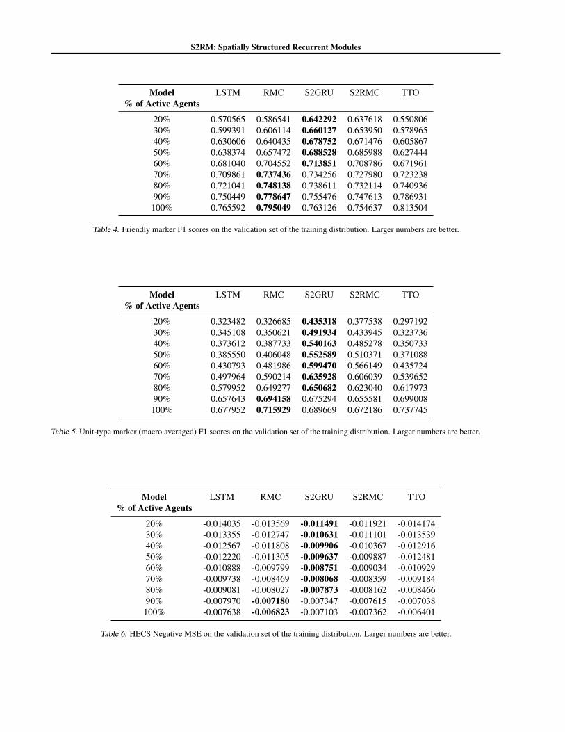
S2RM: Spatially Structured Recurrent Modules
Model LSTM RMC S2GRU S2RMC TTO% of Active Agents
20% 0.570565 0.586541 0.642292 0.637618 0.55080630% 0.599391 0.606114 0.660127 0.653950 0.57896540% 0.630606 0.640435 0.678752 0.671476 0.60586750% 0.638374 0.657472 0.688528 0.685988 0.62744460% 0.681040 0.704552 0.713851 0.708786 0.67196170% 0.709861 0.737436 0.734256 0.727980 0.72323880% 0.721041 0.748138 0.738611 0.732114 0.74093690% 0.750449 0.778647 0.755476 0.747613 0.786931
100% 0.765592 0.795049 0.763126 0.754637 0.813504
Table 4. Friendly marker F1 scores on the validation set of the training distribution. Larger numbers are better.
Model LSTM RMC S2GRU S2RMC TTO% of Active Agents
20% 0.323482 0.326685 0.435318 0.377538 0.29719230% 0.345108 0.350621 0.491934 0.433945 0.32373640% 0.373612 0.387733 0.540163 0.485278 0.35073350% 0.385550 0.406048 0.552589 0.510371 0.37108860% 0.430793 0.481986 0.599470 0.566149 0.43572470% 0.497964 0.590214 0.635928 0.606039 0.53965280% 0.579952 0.649277 0.650682 0.623040 0.61797390% 0.657643 0.694158 0.675294 0.655581 0.699008
100% 0.677952 0.715929 0.689669 0.672186 0.737745
Table 5. Unit-type marker (macro averaged) F1 scores on the validation set of the training distribution. Larger numbers are better.
Model LSTM RMC S2GRU S2RMC TTO% of Active Agents
20% -0.014035 -0.013569 -0.011491 -0.011921 -0.01417430% -0.013355 -0.012747 -0.010631 -0.011101 -0.01353940% -0.012567 -0.011808 -0.009906 -0.010367 -0.01291650% -0.012220 -0.011305 -0.009637 -0.009887 -0.01248160% -0.010888 -0.009799 -0.008751 -0.009034 -0.01092970% -0.009738 -0.008469 -0.008068 -0.008359 -0.00918480% -0.009081 -0.008027 -0.007873 -0.008162 -0.00846690% -0.007970 -0.007180 -0.007347 -0.007615 -0.007038
100% -0.007638 -0.006823 -0.007103 -0.007362 -0.006401
Table 6. HECS Negative MSE on the validation set of the training distribution. Larger numbers are better.
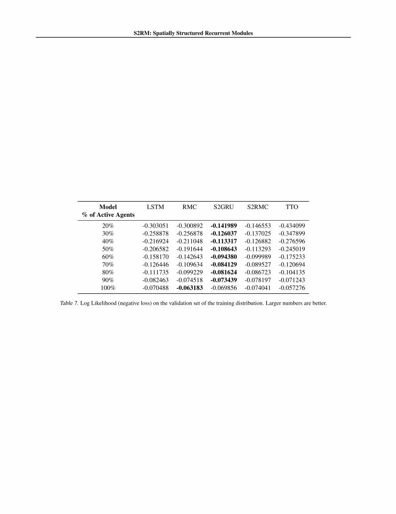
S2RM: Spatially Structured Recurrent Modules
Model LSTM RMC S2GRU S2RMC TTO% of Active Agents
20% -0.303051 -0.300892 -0.141989 -0.146553 -0.43409930% -0.258878 -0.256878 -0.126037 -0.137025 -0.34789940% -0.216924 -0.211048 -0.113317 -0.126882 -0.27659650% -0.206582 -0.191644 -0.108643 -0.113293 -0.24501960% -0.158170 -0.142643 -0.094380 -0.099989 -0.17523370% -0.126446 -0.109634 -0.084129 -0.089527 -0.12069480% -0.111735 -0.099229 -0.081624 -0.086723 -0.10413590% -0.082463 -0.074518 -0.073439 -0.078197 -0.071243
100% -0.070488 -0.063183 -0.069856 -0.074041 -0.057276
Table 7. Log Likelihood (negative loss) on the validation set of the training distribution. Larger numbers are better.