
Spatially variant morphological restoration and skeleton representation
Upload
khangminh22Category
view
3download
0
Modelling, Distributed Identification and Control
of Spatially-Distributed Systems
with Application to an Actuated Beam
Vom Promotionsausschuss derTechnischen Universitat Hamburg-Harburgzur Erlangung des akademischen Grades
Doktor-Ingenieuringenehmigte Dissertation
von
Qin Liu
aus Suining, Sichuan, China
2015

i
1. Gutachter:Prof. Dr. Herbert Werner
2. Gutachter:Prof. Dr.-Ing. Uwe Weltin
Vorsitzende des Promotionsverfahrens:Prof. Dr. sc. techn. Christian Schuster
Tag der mundlichen Prufung: 08.06.2015
urn:nbn:de:gbv:830-88213106

TO MY FAMILY
Contents
Abstract vii
Acknowledgement ix
1 Introduction 1
1.1 Spatially-Distributed Systems . . . . . . . . . . . . . . . . . . . . . . . . . 1
1.1.1 Control Architectures . . . . . . . . . . . . . . . . . . . . . . . . . . 2
1.1.2 Construction of a Distributed System . . . . . . . . . . . . . . . . . 3
1.1.3 Linear Parameter-Varying in Distributed Systems . . . . . . . . . . 4
1.2 Relevant Work in the Field . . . . . . . . . . . . . . . . . . . . . . . . . . . 6
1.2.1 Modelling/Identification . . . . . . . . . . . . . . . . . . . . . . . . 6
1.2.2 Distributed Control . . . . . . . . . . . . . . . . . . . . . . . . . . . 7
1.2.3 Anti-Windup Compensator . . . . . . . . . . . . . . . . . . . . . . 8
1.3 Scope and Main Contributions of this Thesis . . . . . . . . . . . . . . . . . 8
1.4 Thesis Outline . . . . . . . . . . . . . . . . . . . . . . . . . . . . . . . . . . 9
2 Spatially-Interconnected Systems 12
2.1 Introduction . . . . . . . . . . . . . . . . . . . . . . . . . . . . . . . . . . . 12
2.2 Relevant Definitions . . . . . . . . . . . . . . . . . . . . . . . . . . . . . . 12
2.3 Interconnected Systems . . . . . . . . . . . . . . . . . . . . . . . . . . . . . 14
2.3.1 LTSI Systems . . . . . . . . . . . . . . . . . . . . . . . . . . . . . . 15
2.3.2 LTSV Systems . . . . . . . . . . . . . . . . . . . . . . . . . . . . . 16
2.4 Controller Structure . . . . . . . . . . . . . . . . . . . . . . . . . . . . . . 18
2.4.1 LTSI Systems . . . . . . . . . . . . . . . . . . . . . . . . . . . . . . 18
2.4.2 LTSV Systems . . . . . . . . . . . . . . . . . . . . . . . . . . . . . 19
2.5 Well-Posedness, Stability and Performance . . . . . . . . . . . . . . . . . . 21
2.5.1 Well-Posedness . . . . . . . . . . . . . . . . . . . . . . . . . . . . . 21
iii
CONTENTS iv
2.5.2 Exponential Stability and Quadratic Performance . . . . . . . . . . 22
2.6 Summary . . . . . . . . . . . . . . . . . . . . . . . . . . . . . . . . . . . . 24
3 Physical Modelling 25
3.1 Introduction . . . . . . . . . . . . . . . . . . . . . . . . . . . . . . . . . . . 25
3.2 Piezoelectric Effect . . . . . . . . . . . . . . . . . . . . . . . . . . . . . . . 26
3.3 Piezoelectric Actuators/Sensors . . . . . . . . . . . . . . . . . . . . . . . . 27
3.3.1 Piezoelectric Patch Profile . . . . . . . . . . . . . . . . . . . . . . . 27
3.3.2 Functionality as Actuator . . . . . . . . . . . . . . . . . . . . . . . 28
3.3.3 Functionality as Sensor . . . . . . . . . . . . . . . . . . . . . . . . . 28
3.4 Piezoelectric Finite Element Modelling . . . . . . . . . . . . . . . . . . . . 30
3.4.1 FE Discretization . . . . . . . . . . . . . . . . . . . . . . . . . . . . 30
3.4.2 Modelling Based on Euler-Bernoulli Beam Theory . . . . . . . . . . 31
3.5 Updating the FE Model Using the Experimental Modal Analysis . . . . . . 35
3.5.1 Performing Experiments to Obtain FRFs . . . . . . . . . . . . . . . 36
3.5.2 Updating the Mass and Stiffness Matrices . . . . . . . . . . . . . . 38
3.5.3 Updating the Damping Matrix . . . . . . . . . . . . . . . . . . . . . 39
3.5.4 Compensation of the Direct Feed-Through Effect . . . . . . . . . . 41
3.6 Summary . . . . . . . . . . . . . . . . . . . . . . . . . . . . . . . . . . . . 43
4 Local LPV Identification of an FRF Matrix 46
4.1 Introdution . . . . . . . . . . . . . . . . . . . . . . . . . . . . . . . . . . . 46
4.2 Preliminaries . . . . . . . . . . . . . . . . . . . . . . . . . . . . . . . . . . 47
4.2.1 Least-Squares Based Identification . . . . . . . . . . . . . . . . . . 47
4.2.2 LPV Input/Output Identification . . . . . . . . . . . . . . . . . . . 49
4.3 Problem Statement . . . . . . . . . . . . . . . . . . . . . . . . . . . . . . . 51
4.4 LPV Identification of an FRF Matrix . . . . . . . . . . . . . . . . . . . . . 53
4.4.1 Spatially-Varying Characteristics of FRFs . . . . . . . . . . . . . . 53
4.4.2 A Spatial LPV Representation . . . . . . . . . . . . . . . . . . . . . 57
4.5 Experimental Results . . . . . . . . . . . . . . . . . . . . . . . . . . . . . . 61
4.5.1 Ideal Case . . . . . . . . . . . . . . . . . . . . . . . . . . . . . . . . 62
4.5.2 Non-ideal Case . . . . . . . . . . . . . . . . . . . . . . . . . . . . . 63
4.6 Summary . . . . . . . . . . . . . . . . . . . . . . . . . . . . . . . . . . . . 63
5 Distributed Identification 65
CONTENTS v
5.1 Introduction . . . . . . . . . . . . . . . . . . . . . . . . . . . . . . . . . . . 65
5.2 Mathematical Model for Identification . . . . . . . . . . . . . . . . . . . . 66
5.2.1 FD Method to Solve PDEs . . . . . . . . . . . . . . . . . . . . . . . 66
5.2.2 Two-Dimensional Input/Output Model Structure . . . . . . . . . . 69
5.3 Black-Box Identification . . . . . . . . . . . . . . . . . . . . . . . . . . . . 70
5.3.1 Identification of LTSI Models . . . . . . . . . . . . . . . . . . . . . 71
5.3.2 Reasons to Use Spatial LPV Models . . . . . . . . . . . . . . . . . 72
5.3.3 Identification of Spatial LPV Models . . . . . . . . . . . . . . . . . 72
5.3.4 Experimental Identification . . . . . . . . . . . . . . . . . . . . . . 74
5.4 Identification based on the FE Modelling Results . . . . . . . . . . . . . . 75
5.4.1 PDE-Based Selection of Masks . . . . . . . . . . . . . . . . . . . . . 78
5.4.2 Identification of LTSI Models . . . . . . . . . . . . . . . . . . . . . 80
5.4.3 Identification of Spatial LPV Models . . . . . . . . . . . . . . . . . 83
5.5 Summary . . . . . . . . . . . . . . . . . . . . . . . . . . . . . . . . . . . . 86
6 Distributed Controller Design 87
6.1 Introduction . . . . . . . . . . . . . . . . . . . . . . . . . . . . . . . . . . . 87
6.2 Multidimensional State Space Realization . . . . . . . . . . . . . . . . . . . 88
6.2.1 LTSI Models . . . . . . . . . . . . . . . . . . . . . . . . . . . . . . 89
6.2.2 Spatial LPV Models . . . . . . . . . . . . . . . . . . . . . . . . . . 90
6.3 Construction of a Generalized Plant . . . . . . . . . . . . . . . . . . . . . . 93
6.4 Controller Synthesis for LTSI Models . . . . . . . . . . . . . . . . . . . . . 95
6.4.1 Analysis and Synthesis Conditions . . . . . . . . . . . . . . . . . . 95
6.4.2 Decentralized Controller Design . . . . . . . . . . . . . . . . . . . . 99
6.4.3 Experimental Results . . . . . . . . . . . . . . . . . . . . . . . . . . 99
6.5 Controller Synthesis for Temporal/Spatial LPV Models . . . . . . . . . . . 102
6.5.1 Analysis and Synthesis Conditions Using CLFs . . . . . . . . . . . 103
6.5.2 Synthesis Conditions Using PDLFs . . . . . . . . . . . . . . . . . . 107
6.5.3 Experimental Results . . . . . . . . . . . . . . . . . . . . . . . . . . 111
6.6 Summary . . . . . . . . . . . . . . . . . . . . . . . . . . . . . . . . . . . . 111
7 Distributed Anti-Windup Compensator Design 114
7.1 Introduction . . . . . . . . . . . . . . . . . . . . . . . . . . . . . . . . . . . 114
7.2 Preliminary . . . . . . . . . . . . . . . . . . . . . . . . . . . . . . . . . . . 115

7.2.1 AW Scheme for Lumped Systems . . . . . . . . . . . . . . . . . . . 115
7.2.2 Robust Analysis Using IQCs . . . . . . . . . . . . . . . . . . . . . . 116
7.3 Distributed AW Compensator Scheme . . . . . . . . . . . . . . . . . . . . 119
7.3.1 Analysis Conditions . . . . . . . . . . . . . . . . . . . . . . . . . . . 122
7.3.2 Synthesis Conditions . . . . . . . . . . . . . . . . . . . . . . . . . . 123
7.4 Decentralized AW Compensator Design . . . . . . . . . . . . . . . . . . . . 125
7.5 Simulation Results . . . . . . . . . . . . . . . . . . . . . . . . . . . . . . . 125
7.6 Summary . . . . . . . . . . . . . . . . . . . . . . . . . . . . . . . . . . . . 129
8 Conclusions and Outlook 132
A State Space Realization of Identified Models 136
A.1 LTSI Models . . . . . . . . . . . . . . . . . . . . . . . . . . . . . . . . . . . 136
A.2 Spatial LPV Models . . . . . . . . . . . . . . . . . . . . . . . . . . . . . . 137
B Proof of Theorem 6.8 139
C Auxiliary Technical Material 143
C.1 Hardware and Software Description . . . . . . . . . . . . . . . . . . . . . . 143
C.2 Upper and Lower LFT . . . . . . . . . . . . . . . . . . . . . . . . . . . . . 143
C.3 Bilinear Transformation . . . . . . . . . . . . . . . . . . . . . . . . . . . . 143
C.4 Elimination Lemma . . . . . . . . . . . . . . . . . . . . . . . . . . . . . . . 144
C.5 KYP Lemma . . . . . . . . . . . . . . . . . . . . . . . . . . . . . . . . . . 145
Bibliography 146
List of Notations, Symbols and Abbreviations 154
List of Publications 159

Abstract
This thesis studies the modelling, distributed identification and control of spatially-distributed systems. The development of light-weight piezoelectric materials enablessensing and actuating distributed systems without significantly changing the dynamicsof the original system. In this work, a flexible structure – a 4.8 m long aluminiumbeam equipped with 16 pairs of collocated piezo actuators and sensors – is constructedfor experimental study. The piezoelectric finite element method that accounts for boththe flexible structure and the distributed piezo pairs is applied to physically model thecoupled electric and elastic dynamics. As an alternative to exploring the physical prop-erties of the actuated structure, a local linear parameter-varying (LPV) identificationapproach is extended from lumped to spatio-temporal systems to identify the frequencyresponse function (FRF) matrix (or the transfer function matrix) by directly modellingits input/output behaviour.
It is well-known that spatially-distributed systems are typically governed by partial dif-ferential equations (PDEs). After spatially discretizing the governing PDE, the systemcan be considered as the interconnection of subsystems, each interacting with its near-est neighbours and equipped with actuating and sensing capabilities. A two-dimensionalinput/output model, which defines the system dynamics on a single subsystem of smallorder, is employed as the mathematical model for the distributed identification of both theparameter-invariant and parameter-varying systems, where the dynamics of the parameter-varying systems can be captured by temporal/spatial LPV models.
To apply the well-developed state-space based synthesis conditions, the experimentallyidentified input/output models are converted into their multidimensional state space rep-resentations that lead to an efficient, linear matrix inequality (LMI)-based synthesis ofdistributed controllers. It is desired that the controller inherits the interconnected struc-ture of the plant. Therefore, a linear time- and space-invariant distributed controller anda temporal/spatial LPV controller are used to control the parameter-invariant and theparameter-varying systems, respectively. To reduce the conservatism caused by the use ofconstant Lyapunov functions in the LPV controller design, analysis and synthesis condi-tions using parameter-dependent Lyapunov functions are proposed by extending previousresults on lumped systems. The designed controllers are tested experimentally in termsof suppressing the disturbances injected to the actuated beam.
Actuator saturation is usually not taken into account when solving the controller syn-thesis problem. To overcome the performance degradation caused by the constrainedactuator capacity, a distributed anti-windup scheme is proposed. The nonlinear satura-
vii

Chapter 0. Abstract viii
tion/deadzone operator is characterized in terms of LMIs using integral quadratic con-straints (IQCs) with a suitable choice of multiplier. The performance of the distributedanti-windup scheme is compared with that of a decentralized anti-windup scheme.

Acknowledgement
This thesis is the conclusion of my four years of research work at the Institute of ControlSystems (ICS), Hamburg University of Technology (TUHH) from 11.2010 to 10.2014. Iwould like to thank those people without whose contributions and support this workwould not have been possible.
I would like to express my sincere gratitude to my supervisor Prof. Herbert Werner, whogave me the chance to start this journey at the first place and guided me through itwith his rich knowledge, vision and patience. Prof. Werner impacted me deeply with hisrigorous research attitude and critical thinking, which have helped me to shape my ownunderstanding of conducting research.
I am also grateful to Prof. Uwe Weltin for his willingness to be the second examiner aswell as his suggestions which helped to broaden this work, and to Prof. Christian Schusteras the president of the doctoral committee.
I would also like to thank all my colleagues at the ICS for the wonderful teamwork andfriendship throughout the years. It was a great experience to work hard together on papersand share the joy after the acceptance. In particular, I am grateful to Annika Eichler,Christian Hoffmann, Antonio Mendez, Dr. Sven Pfeiffer, Simon Wollnack, Fatimah Al-Taie and Dr. Ahsan Ali. The cooperation work and fruitful discussions with them inspiredme and improved my work. Many thanks go to my former colleague Mahdi Hashemi, whowas also the supervisor of my project work and master thesis. Working together with himreinforced my interest in control engineering. I would also like to thank Herwig Meyerfor constructing test-beds for my work and always being helpful when I approached himwith various problems, and Klaus Baumgart and Uwe Jahns for their technical support.Our former secretary Mrs. von Dewitz, and current secretaries Bettina Schrieber andChristine Kopf, who have always been great help, are thankfully acknowledged.
In addition to the aforementioned colleagues, I would like to express my gratitude toDr. Joseph Gross from the Institute for Reliability Engineering, for helping me to learnstructural dynamics and answering my questions with enormous patience.
My warmest thanks go to my parents, who have been encouraging me to build and pursuemy dreams since I was a kid, even if those dreams take me further and further away fromthem. It is their unconditional support and love that make everything possible at all. Iwould like to thank my parents-in-law and brothers-in-law, who care about me like theirown daughter / sister. Last and foremost, I would like to thank my beloved husbandSebastian, who is always there for me. His belief in me gave me the strength and courage
ix

Chapter 0. Acknowledgement x
to accomplish this journey. What this thesis recorded are not only the research resultsthat I have achieved, but also a great time and memory that I will cherish forever.
Chapter 1
Introduction
Spatially-distributed systems, a class of distributed-parameter systems as opposed tolumped parameter systems, arise in various engineering problems. Examples include ve-hicular platoons [1], modern paper-making machines [2], the distribution of heat or fluidin a given region [3], smart materials and structures [4], etc. Variables in lumped systemsare functions of time alone, whereas a common feature of distributed-parameter systemsis their underlying independent temporal and spatial dynamics, i.e. all involved signalsare functions of time and space. Thus, this class of systems is often addressed in theframework of spatio-temporal systems.
The modelling, analysis and control of one typical spatially-distributed system – flexiblestructures – have been extensively studied in structural engineering since decades. Thisthesis addresses these issues in a newly developed framework developing theoretical meth-ods, as well as evaluating them experimentally. This introduction should motivate theproblems to be considered in this work. Main contributions and an outline of this thesisare provided at the end of this chapter.
1.1 Spatially-Distributed Systems
Flexible structures are spatially-continuous systems whose mass and stiffness are functionsof spatial variables. The distributed nature of these systems can be captured using partialdifferential equations (PDEs). Due to the spatial continuum, this class of systems is oftenreferred to as infinite-dimensional systems, indicating the infinite dimension of the statespace. The well-developed semigroup theory [5] has been widely employed for a precisemathematical treatment of the internal dynamics of an infinite-dimensional system, whichis significantly more difficult than the finite-dimensional theory [6].
The active vibration control of flexible structures often involves a large number of spatially-distributed actuators and sensors. Instead of preserving the continuous nature in space,the attachment of actuators and sensors induces a spatial discretization, so that the overallstructure can be treated as a physical interaction between spatially-discretized subsystemson one or multidimensional discrete lattices. A one-dimensional flexible structure after
1

Chapter 1. Introduction 2
the spatial discretization is shown in Fig. 1.1. The dynamics of the spatially-discretizedsubsystems can be modelled by a finite number of coupled ordinary differential equations(ODEs) [7]. Assumed here are the convergence of finite-dimensional approximation, andsensing and actuating capabilities on each subsystem.
Figure 1.1: Subsystems on one-dimensional lattices after the spatial discretization
The fast development of the microelectromechanical system (MEMS) and light-weightpiezoelectric materials makes the manufacturing of large arrays of actuators and sensorsfeasible and economical. Meanwhile, attaching or embedding microscopic devices on thestructural surface enables the spatially-discretized subsystems being equipped with actu-ating, sensing, and even computing and telecommunication capabilities, without changingits nominal dynamics significantly.
1.1.1 Control Architectures
When it comes to the control of these large-scale systems, the choice of the control architec-ture determines the involved computation effort, as well as the closed-loop performance; itthus plays a crucial role. With each subsystem equipped with collocated or non-collocatedactuators and sensors, three prevalent architectures are the centralized, the decentralized,and the localized or so-called distributed control schemes, as shown in Fig. 1.2.
flexible structure
flexible structure
flexible structure
(a)
(b)
(c)
computation unit actuator/sensor
Figure 1.2: Three control architectures for a large-scale system: (a) centralized scheme;(b) decentralized scheme; (c) distributed scheme. Red arrows denote the information flowbetween actuators/sensors and computation units; blue arrows denote the informationflow between computation units.

Chapter 1. Introduction 3
• Centralized scheme: A centralized control scheme, as shown in Fig. 1.2 (a), treatsthe distributed system as a lumped system with multiple-input and multiple-output(MIMO). The computation unit – often a central computer – requires the connectionwith all sensors and actuators. A centralized controller normally possesses a largesystem order. In many cases it fails to realize an effective control due to a high levelof connectivity and computational burden. It is more sensitive to actuator/sensorfailures and transmission errors.
• Decentralized scheme: Instead of communicating with a central computer, eachsubsystem in a decentralized control scheme as shown in Fig. 1.2 (b) is equipped withan independent computation unit executing controller algorithms. It receives thesensing information from its located subsystem, and actuates at the same location.The controller of a decentralized scheme handles the dynamics of a single subsystemof a significantly smaller order compared to that of a centralized system.
• Distributed (localized) scheme: It has been shown in [6], that a spatially-distributedsystem exhibits some degrees of localization. A distributed control scheme inheritsthe spatial structure of the plant, where the computation units interact with nearestneighbours as shown in Fig. 1.2 (c). It is different from the decentralized scheme inthe sense that the distributed controller exchanges information with the subsystemwhere it locates, as well as with neighbouring subsystems. In both decentralizedand distributed schemes, none of the controller subsystems has the information ofthe complete system, whereas the communication among subsystems in Fig. 1.2 (c)enables an improved overall performance compared to Fig. 1.2 (b). Thus, the dis-tributed scheme is considered superior to the other two architectures.
1.1.2 Construction of a Distributed System
Inspired by the works [6] [8], an actuated flexible structure as shown in Fig. 1.3 hasbeen constructed to study the behaviour of a spatially-distributed system. The flexiblestructure—an aluminium beam measuring 4.8 m in length, 4 cm in width, and 3 mm inthickness, is equipped with 16 paris of piezoelectric actuators and sensors in collocatedpattern. A zoomed-in collocated piezo pair is shown in Fig. 1.4, where the piezo patch onthe top functions as actuator, the one at the bottom as sensor.
In order to approximate a free-body suspension condition, where the resonant frequenciesof the rigid body modes are at least half of that of the first bending mode [9], 17 softsprings are used to suspend the structure in parallel. A schematic drawing of the test bedis shown in Fig. 1.5.
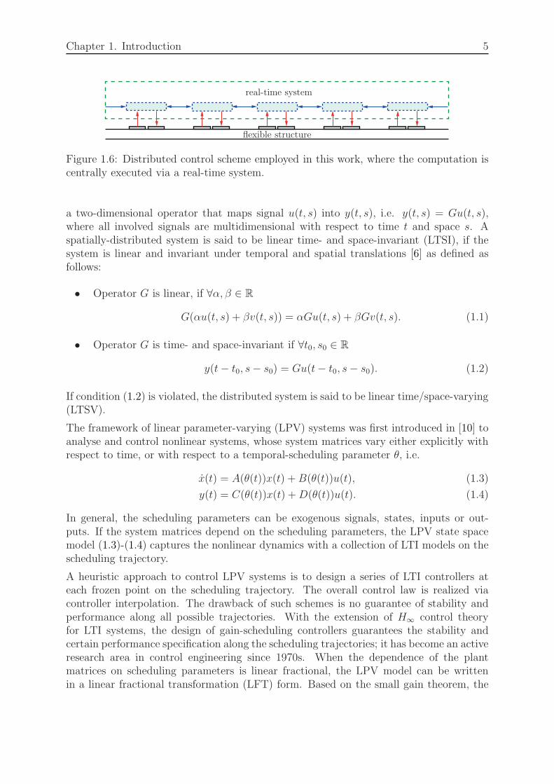
The attachment of distributed actuators and sensors virtually divides the structure into16 spatially-interconnected subsystems, each equipped with actuating and sensing capa-bilities. This thesis is meant to experimentally test the distributed control scheme inFig. 1.2 (c) due to its superiority. However, constructing 16 physically parallel computa-tion units requires a large amount of expense and effort. Instead, a much cheaper solutionas shown in Fig. 1.6 has been employed by using a centralized real-time system to real-

Chapter 1. Introduction 4
(a) (b)
Figure 1.3: The experimental setup: (a) downward view of 16 actuators; (b) upward viewof 16 sensors
Figure 1.4: One collocated piezo actuator/sensor pair
Figure 1.5: A schematic drawing of the experimental setup
ize the computation tasks of 16 parallel units, with the distributed nature of controllersstill preserved. The main hardware and software components are listed in Table C.1 (seeAppendix C).
1.1.3 Linear Parameter-Varying in Distributed Systems
After the spatial discretization, the resulting subsystems may exhibit identical or varyingdynamics. Analogous to the definition of linear time-invariant (LTI) systems, let G be
Chapter 1. Introduction 5
flexible structure
real-time system
Figure 1.6: Distributed control scheme employed in this work, where the computation iscentrally executed via a real-time system.
a two-dimensional operator that maps signal u(t, s) into y(t, s), i.e. y(t, s) = Gu(t, s),where all involved signals are multidimensional with respect to time t and space s. Aspatially-distributed system is said to be linear time- and space-invariant (LTSI), if thesystem is linear and invariant under temporal and spatial translations [6] as defined asfollows:
• Operator G is linear, if ∀α, β ∈ R
G(αu(t, s) + βv(t, s)) = αGu(t, s) + βGv(t, s). (1.1)
• Operator G is time- and space-invariant if ∀t0, s0 ∈ R
y(t− t0, s− s0) = Gu(t− t0, s− s0). (1.2)
If condition (1.2) is violated, the distributed system is said to be linear time/space-varying(LTSV).
The framework of linear parameter-varying (LPV) systems was first introduced in [10] toanalyse and control nonlinear systems, whose system matrices vary either explicitly withrespect to time, or with respect to a temporal-scheduling parameter θ, i.e.
x(t) = A(θ(t))x(t) +B(θ(t))u(t), (1.3)
y(t) = C(θ(t))x(t) +D(θ(t))u(t). (1.4)
In general, the scheduling parameters can be exogenous signals, states, inputs or out-puts. If the system matrices depend on the scheduling parameters, the LPV state spacemodel (1.3)-(1.4) captures the nonlinear dynamics with a collection of LTI models on thescheduling trajectory.
A heuristic approach to control LPV systems is to design a series of LTI controllers ateach frozen point on the scheduling trajectory. The overall control law is realized viacontroller interpolation. The drawback of such schemes is no guarantee of stability andperformance along all possible trajectories. With the extension of H∞ control theoryfor LTI systems, the design of gain-scheduling controllers guarantees the stability andcertain performance specification along the scheduling trajectories; it has become an activeresearch area in control engineering since 1970s. When the dependence of the plantmatrices on scheduling parameters is linear fractional, the LPV model can be writtenin a linear fractional transformation (LFT) form. Based on the small gain theorem, the

Chapter 1. Introduction 6
existence of a gain-scheduled controller is fully characterized in terms of linear matrixinequalities (LMIs) [11] [12], via searching for Lyapunov functions that establish stabilityand performance of the closed-loop system. The use of constant Lyapunov functions(CLFs) allows for arbitrarily fast parameter variations, thus resulting conservatism inthe case of slowly varying parameters. To reduce the conservatism caused by the use ofCLFs, an improvement can be expected by exploiting the concept of parameter-dependentLyapunov functions (PDLFs), which allows to incorporate the knowledge on the rate ofparameter variations in the derivation of analysis and synthesis conditions [13] [14] [15].A more detailed overview regarding LPV systems and LPV controller design can be foundin [16] [17] [18] [19] [20].
Although the LPV framework was first introduced to deal with time-varying systems,it can be extended in a straightforward way to solve analogous problems in distributedsystems with varying parameters. If the system matrices can be parametrized as functionsof temporal- and/or spatial-scheduling parameters, a temporal/spatial LPV model can beused to capture the structural dynamics over the multidimensional variation range. Thecontroller design techniques developed for temporal LPV models can be extended andapplied to LTSV models [21].
1.2 Relevant Work in the Field
Theoretical approaches for the modelling, analysis and control of spatially-distributedsystems have been developed in numerous works. This section reviews some of themwhich are relevant to the topics concerned in this thesis, and motivates problems to beaddressed.
1.2.1 Modelling/Identification
Modelling of continuous structures has been a routine topic of research in structural en-gineering for decades. The finite element (FE) method [22], as a numerical modellingapproach, has been employed extensively in the theoretical analysis of structural be-haviour in aeronautics, civil and building structures, biomechanical problems, automotiveapplications and so on. The standard FE method accounts only for the mechanical energydissipation, not taking the bonded piezo actuators/sensors – parts of the experimentalsetup in Section 1.1.2 – into consideration. The piezoelectric effect was first incorporatedinto the FE modelling in [23] and [24]. The derived piezoelectric FE approach takes careof coupled piezoelectric and elastic effect, and has been widely applied to the modellingof intelligent structures in [25] [26], etc.
Modelling using the FE method helps to understand the physical behaviour of the struc-ture, taking safety and reliability issues into consideration. However, with the increase ofstructural complexity, the FE modelling can become expensive and involves large compu-tation effort. Meanwhile, the obtained FE model treats the structure as a lumped MIMO

Chapter 1. Introduction 7
system; the resulting large system order makes it unfavourable for further controller de-sign.
In contrast, black-box identification out of experimental measurements does not requirea prior knowledge on the principle laws of physics; it thus serves as a fast and efficientsolution. It is well-known, that the dynamics of continuous structures are typically gov-erned by PDEs. The temporal and spatial discretization of a governing PDE leads to atwo-dimensional input/output model, which could be used as the mathematical model forblack-box identification. Based on the least-squares estimation, a black-box identificationapproach for LTSI systems has been developed in [27]. The identified model defines thedynamics of a single subsystem interacting with its neighbouring subsystems, with thelocalized nature of the plant preserved. In the presence of temporal/spatial variations, thetemporal LPV input/output identification techniques proposed in [28] have been extendedin [29] for the identification of temporal/spatial LPV models.
1.2.2 Distributed Control
Since last few decades, the design of distributed controllers that preserve the distributedstructure of the plant as shown in Fig. 1.7 has received extensive attentions. Severalframeworks have been proposed to address this issue from different perspectives [8] [30][31] [32], etc. Two common features of these approaches are: 1. the overall system istreated as the interconnection of small-order subsystems; 2. the controller inherits thecommunication topology of the plant.
GGGGGG
KKKKKK
Figure 1.7: Distributed controller designed for a distributed plant
Among them, [8] introduced a novel multidimensional state space model to representthe interconnected dynamics of an LTSI system. Analysis and synthesis conditions areformulated in terms of LMIs, using the induced L2 norm as the performance criterion.To investigate the effectiveness of the framework proposed in [8], a simulation case studyon the distributed control of a flexible beam has been performed in [33]. Accounting forthe boundary conditions, non-uniform physical characteristics of the structure, etc., toolshave been developed in [21] [34] to solve the control problem when the underlying systemdynamics are not invariant with respect to temporal or spatial variables.
The distributed control scheme has been perceived as an effective and computationallyattractive solution to tackle large-scale distributed systems. Among the various developedapproaches, very few of them have been validated experimentally. This thesis is meant to
Chapter 1. Introduction 8
fill in this gap by exploring the experimental implementation of the framework proposedin [8] on the constructed test structure.
1.2.3 Anti-Windup Compensator
In all physical systems, actuator capacities are limited by the inherent physical constraintsand limitations of the actuators. In the presence of actuator saturation, any controllerwith slow or unstable dynamics exhibits a windup effect [35]: the established closed-loopperformance suffers from deterioration, or even instability. The design of an effectiveanti-windup (AW) compensator for lumped systems has been an active field of researchsince 1970s. Only in the last decade, a more formal way with stability and performancespecifications incorporated in the AW design has been established using H∞ optimalcontrol [36]. In recent years, LMIs are employed as a tool to impose constraints on thedesign of an AW compensator [37] [38] [39], which significantly simplifies the computationof the global optimal solution into a convex optimization problem.
The windup effect can arise in distributed systems as well. Saturation on one actua-tor could easily lead to saturation on an array of interconnected actuators. Until now,very few works have addressed this issue thoroughly [40] [41]. Taking the inherent dis-tributed dynamics of the plant and the controller into consideration, an appropriate AWscheme could effectively alleviate the degradation of the closed-loop performance causedby actuator saturation, thus being worth further research.
1.3 Scope and Main Contributions of this Thesis
This thesis focuses on the modelling, distributed identification and control of spatially-interconnected systems, with an application to an aluminium beam equipped with an arrayof collocated piezo actuator and sensor pairs. For a better understanding of the underlyingphysical laws of the test structure, it is meaningful to start with the physical modellingbased on the knowledge of its properties and functionalities. Furthermore, the distributedframework proposed in [8] is employed in this thesis for the system analysis and distributedcontroller design. In order to apply the well-developed analysis and synthesis conditionsdeveloped in [8], a distributed model in multidimensional state space form needs to beidentified first. Considered in this thesis are both the LTSI and LTSV systems. By slightlymodifying the hardware, the test structure can realize the configurations required for boththe LTSI and LTSV models. It is desired, that the controller inherits the interconnectedstructure of the plant as shown in Fig. 1.7. The distributed control problem of boththe identified LTSI and LTSV models are addressed, and implemented experimentally.Keeping the physical limitations of the distributed actuators in mind, an appropriateAW scheme that accounts for the distributed nature of the plant and the controller, caneffectively counteract the windup effect with a bound on the closed-loop performanceguaranteed in the presence of actuator saturation.
Chapter 1. Introduction 9
The main contributions of this thesis are summarized as follows:
• The piezoelectric FE modelling approach is applied to model the coupled piezo-electric and mechanical behaviour of the piezo-actuated beam structure. With thecombined implementation of the experimental modal analysis, an FE model thatcaptures the structural dynamics of the real plant to a satisfactory degree is ob-tained.
• Frequency response function (FRF) is a mathematical representation of the rela-tionship from an excitation at one location to the vibration response at the same oranother location. It is demonstrated, that FRFs of even a homogeneous structureexhibit spatially-varying characteristics. A local LPV input/output identificationtechnique for temporal systems is extended to spatio-temporal systems to model theFRF matrix as a spatial LPV model based on black-box identification.
• The multidimensional black-box identification techniques developed in [27] for LTSImodels and [29] for spatial LPV models are for the first time implemented exper-imentally. Although the identified models capture the structural behaviour to acertain extent, dynamics at resonances are hardly identified. A new identificationprocedure is proposed to extract a distributed input/output model from the ob-tained FE model, yielding improved identification results.
• Distributed LTSI and LPV controllers for the LTSI and for the LTSV systems aredesigned, respectively, and experimentally implemented to suppress the vibratorymotion of the actuated beam caused by the disturbance injection. To reduce the con-servatism with the use of CLFs, the LPV controller design technique using PDLFsis extended from lumped systems to spatially-distributed systems with varying pa-rameters. The performance of the designed controllers is evaluated experimentally.
• To alleviate the windup effect due to actuator saturation, a distributed AW scheme,that inherits the distributed pattern of the controlled system is proposed. Thedesigned AW compensator can be implemented on top of an existing closed-loopsystem, with the global stability and a bound on L2 performance of the constrainedsystem guaranteed.
1.4 Thesis Outline
This thesis consists of eight chapters. A brief overview of the content in each chapter isgiven below:
Chapter 2 reviews the framework of spatially-interconnected systems. Definitions onthe multidimensional signal and system norms are given as a preliminary. The multidi-mensional state space representations, that are employed throughout the work, proposedin [8] for LTSI systems, in [21] for LTSV systems, as well as their correspondent con-trollers, which inherit the distributed nature of the plant, are presented. The definitionsof the well-posedness, exponential stability, and quadratic performance in the context

Chapter 1. Introduction 10
of distributed systems are discussed. The analysis conditions for an LTSI system to bewell-posed, exponentially stable, and with the imposed performance criteria satisfied areprovided for both continuous and discrete systems.
Chapter 3 takes physical aspects of the experimental structure into consideration, re-viewing the functionality of piezoelectric patches as actuator and sensor, respectively.Linear constitutive equations are applied to analyse the linear dynamics of both the piezoactuators and sensors. The application of a piezoelectric FE modelling approach yieldsa theoretical FE model characterized in terms of mass and stiffness matrices, based onknown and assumed knowledge on the physical properties of the actuated beam. Toreduce the deviation between the theoretical FE model and test structure, experimen-tal modal analysis is performed to update the mass and stiffness matrices at first, thenthe proportional-assumed damping matrix. Meanwhile, a direct feed-through effect isobserved from actuators to collocated sensors.
Instead of exploring the inherent physics of a flexible structure using the FE mod-elling, Chapter 4 identifies a structure through identifying its FRF matrix from theinput/output measurements. It is demonstrated step by step, that even for a structurecomprised of identical subsystems, its FRF matrix exhibits spatially-varying character-istics. A local LPV identification technique for temporal systems is extended to spatio-temporal systems to capture the spatially-varying properties of FRFs. Actuating andsensing at selected locations results in a set of measured FRFs, each being estimated asan LTI model using a least-squares-based identification technique. The application of theextended local LPV approach parametrizes the set of estimated LTI models as a spa-tial LPV model by defining the spatial coordinates of actuating and sensing locations asspatial scheduling parameters. The proposed approach allows to perform identification ex-periments at a small number of selected actuating and sensing locations, and parametrizea spatial LPV model. Then unknown FRFs at other locations can be easily approximatedthrough interpolation. The proposed approach is tested experimentally.
Both the obtained FE model in Chapter 3 and the identified FRF matrix in spatial LPVrepresentation in Chapter 4 treat the plant as a MIMO lumped system. Chapter 5 dealswith the identification problem in the context of spatially-distributed systems. A two-dimensional input/output model induced by the temporal and spatial discretization ofgoverning PDEs is considered as the mathematical model for identification. It describesthe dynamics of a spatially-discrete subsystem interacting with nearby subsystems. Black-box identification techniques for the identification of LTSI and LTSV models are brieflyreviewed, and experimentally implemented. To improve the model accuracy, especially atresonant peaks, a new identification procedure which makes use of the FE model obtainedin Chapter 3 is proposed. Both the identified LTSI and spatial LPV models preserve thetwo-dimensional input/output structure, and suggest a better representation of the plantdynamics than black-box identification.
Based on the input/output models identified in Chapter 5, Chapter 6 solves the con-troller design problem for both the LTSI and LTSV systems. In order to employ thewell-developed state-space based analysis and synthesis conditions, the experimentallyidentified input/output models are first converted into their multidimensional state space
Chapter 1. Introduction 11
realizations. The construction of a multidimensional generalized plant for shaping themixed sensitivity of the closed-loop system is discussed. The synthesis conditions of adistributed LTSI controller are briefly reviewed. Both a distributed and a decentralizedcontroller are designed and implemented, with their performance compared experimen-tally. The synthesis conditions of temporal/spatial LPV controllers for LTSV systems arederived with the application of the full block S-procedure (FBSP), using both the CLFsand PDLFs. The experimental results demonstrate a superior performance of the LPVcontroller designed using PDLFs.
Chapter 7 addresses a two-step distributed AW compensator design in the presence ofactuator saturation in physical systems. A lumped AW scheme is first revisited. Thedefinition of a mathematical tool – integral quadratic constraints (IQCs) [42] – and itsapplication to the robust analysis of an LFT model with a nonlinear uncertainty is shortlyrecapped. Inspired by the lumped setup, a distributed AW scheme, which preserves thedistributed nature of the plant and the controller, is proposed. The stability of theclosed-loop subsystem in LFT form, with the nonlinear deadzone operator as uncertainty,is analysed using IQCs. The synthesis conditions are derived after applying the elimina-tion lemma. The performance of the distributed AW compensator is illustrated using asimulation example, in comparison with a decentralized AW scheme.
In Chapter 8, conclusions to this thesis are drawn; and an outlook for future research isgiven.
Chapter 2
Spatially-Interconnected Systems
2.1 Introduction
In this chapter, relevant preliminary materials regarding spatially-interconnected systemsare briefly reviewed. In Section 2.2, signal and system norms and shift operators in thecontext of spatially-interconnected systems are extended from their lumped counterparts.Instead of considering the distributed-parameter system as a large-scale lumped MIMOsystem, the distributed framework proposed in [8], where a spatially-distributed systemcan be seen as an array of interconnected subsystems, is presented in Section 2.3. Thesystem dynamics are defined at the subsystem level using a multidimensional state spacerepresentation. Depending on the physical properties of subsystems, such a system canbe either LTSI or LTSV, where subsystems in an LTSI system share identical dynamics,whereas the varying dynamics of an LTSV system can be captured using temporal/spatial-LPV models. It is desired that the controller inherits the distributed feature of the plant.The controller structures for both parameter-invariant and parameter-varying systemsare given in Section 2.4. In Section 2.5, the well-posedness, exponential stability andquadratic performance are defined for spatially-interconnected systems, respectively. Theanalysis conditions that establish well-posedness, stability and performance specificationsare stated in terms of LMIs.
2.2 Relevant Definitions
Unlike lumped systems, whose signals are functions of time only, spatially-distributedsystems are multidimensional systems. For systems in L spatial dimensions, involvedsignals are indexed by L + 1 independent variables, e.g. signal u(k, s1, s2, . . . , sL) withrespect to discrete temporal variable k, and discrete spatial variables s1, s2, . . . , sL, wheresi indexes the i-th spatial dimension. This work focuses on distributed systems of onespatial dimension, i.e. u(k, s).
Signal norms for lumped systems measure the size of a signal over time, whereas systemnorms measure the gain of a system. These measures apply to multidimensional systems
12
Chapter 2. Spatially-Interconnected Systems 13
as well. The normed spaces, the signal and space norms, as well as the shift operators,have been extended to spatially-distributed systems in [8], accounting for both temporaland spatial variables.
Definition 2.1 (Inner Product Space [5]) An inner product on a linear vector spaceV defined over complex or real filed F is a map
< ·, · >: V × V → F . (2.1)
Definition 2.2 (Hilbert Space [5]) A Hilbert space is an inner product space that iscomplete as a normed linear space under the induced norm.
The spaces l2 and L2 are Hilbert spaces under inner products. Provided x(k, s)—a func-tion of discrete time k and discrete space s, the spaces l2 and L2 are defined by separatingthe spatial and temporal parts of the signal as follows:
Definition 2.3 (Space l2 [8]) The space l2 is the set of functions that the followingquantity with fixed temporal variable k = k0
∞∑
s=−∞
xT (k0, s)x(k0, s) (2.2)
is bounded.
The corresponding l2 norm is defined as
‖ x(k0, s) ‖2l2 :=∞∑
s=−∞
xT (k0, s)x(k0, s). (2.3)
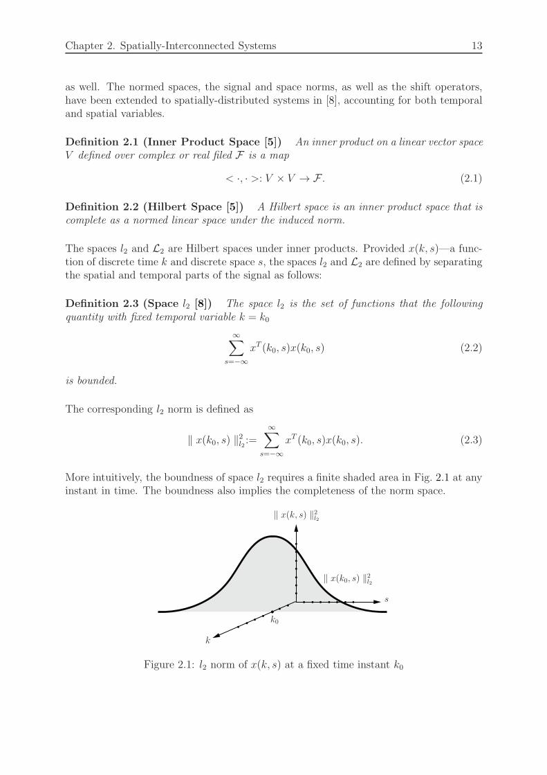
More intuitively, the boundness of space l2 requires a finite shaded area in Fig. 2.1 at anyinstant in time. The boundness also implies the completeness of the norm space.
k
s
‖ x(k, s) ‖2l2
k0
‖ x(k0, s) ‖2l2
Figure 2.1: l2 norm of x(k, s) at a fixed time instant k0
Chapter 2. Spatially-Interconnected Systems 14
Provided that x(k, s) is in l2, the space L2 assesses the boundness of x(k, s) over the wholepositive time.
Definition 2.4 (Space L2 [8]) The space L2 is defined as the set of functions forwhich the following quantity
∞∑
k=1
∞∑
s=−∞
xT (k, s)x(k, s) (2.4)
is bounded.
The corresponding L2 norm is defined as
‖ x(k, s) ‖2L2:=
∞∑
k=1
∞∑
s=−∞
xT (k, s)x(k, s). (2.5)
Analogous to lumped systems, the induced L2 norm of a multidimensional system mea-sures the system gain - the maximum ratio from the L2 norm of the output signal to theL2 norm of the input signal.
Definition 2.5 (System Norm [8]) The induced L2 norm of an operator G is definedas
‖ G ‖L2:= sup
x 6=0,x∈L2
‖ Gx ‖L2
‖ x ‖L2
. (2.6)
The operator G is said to be bounded on L2 if ‖ G ‖L2< ∞ holds.
Definition 2.6 (Shift Operators [8]) The temporal forward shift operator T is de-fined as
Tx(k, s) = x(k + 1, s), (2.7)
whereas the spatial forward and backward shift operators S and S−1 act on signals in onespatial dimension as
Sx(k, s) = x(k, s+ 1), S−1x(k, s) = x(k, s− 1). (2.8)
2.3 Interconnected Systems
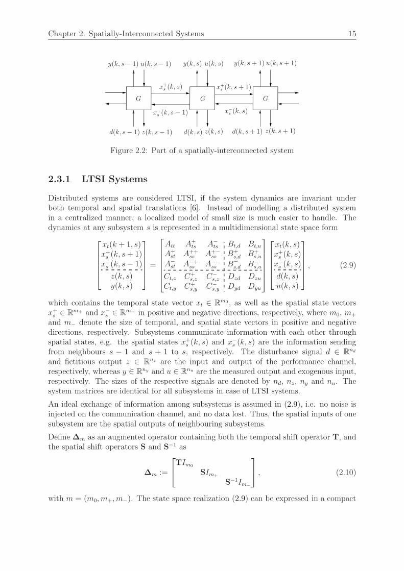
According to the framework proposed in [8], a spatially-distributed system is comprised ofa number of interconnected subsystems exchanging information with their nearest neigh-bours as depicted in Fig. 2.2. The subsystems can either be identical or exhibit differentdynamics, due to the physical properties, boundary conditions of the distributed system,etc. In this section, the multidimensional state space models that describe the dynamicsof both the parameter-invariant and -varying systems are established.
Chapter 2. Spatially-Interconnected Systems 15
G GG
x+s (k, s) x+
s (k, s+ 1)
x−s (k, s− 1) x−
s (k, s)
y(k, s− 1) u(k, s− 1) y(k, s) u(k, s) y(k, s+ 1) u(k, s+ 1)
d(k, s− 1) z(k, s− 1) d(k, s) z(k, s) d(k, s+ 1) z(k, s + 1)
Figure 2.2: Part of a spatially-interconnected system
2.3.1 LTSI Systems
Distributed systems are considered LTSI, if the system dynamics are invariant underboth temporal and spatial translations [6]. Instead of modelling a distributed systemin a centralized manner, a localized model of small size is much easier to handle. Thedynamics at any subsystem s is represented in a multidimensional state space form
xt(k + 1, s)x+s (k, s+ 1)
x−s (k, s− 1)
z(k, s)y(k, s)
=
Att A+ts A−
ts Bt,d Bt,u
A+st A++
ss A+−ss B+
s,d B+s,u
A−st A−+
ss A−−ss B−
s,d B−s,u
Ct,z C+s,z C−
s,z Dzd Dzu
Ct,y C+s,y C−
s,y Dyd Dyu
xt(k, s)x+s (k, s)
x−s (k, s)
d(k, s)u(k, s)
, (2.9)
which contains the temporal state vector xt ∈ Rm0 , as well as the spatial state vectors
x+s ∈ Rm+ and x−
s ∈ Rm− in positive and negative directions, respectively, where m0, m+
and m− denote the size of temporal, and spatial state vectors in positive and negativedirections, respectively. Subsystems communicate information with each other throughspatial states, e.g. the spatial states x+
s (k, s) and x−s (k, s) are the information sending
from neighbours s − 1 and s + 1 to s, respectively. The disturbance signal d ∈ Rnd
and fictitious output z ∈ Rnz are the input and output of the performance channel,respectively, whereas y ∈ Rny and u ∈ Rnu are the measured output and exogenous input,respectively. The sizes of the respective signals are denoted by nd, nz, ny and nu. Thesystem matrices are identical for all subsystems in case of LTSI systems.
An ideal exchange of information among subsystems is assumed in (2.9), i.e. no noise isinjected on the communication channel, and no data lost. Thus, the spatial inputs of onesubsystem are the spatial outputs of neighbouring subsystems.
Define ∆m as an augmented operator containing both the temporal shift operator T, andthe spatial shift operators S and S−1 as
∆m :=
TIm0
SIm+
S−1Im−
, (2.10)
with m = (m0, m+, m−). The state space realization (2.9) can be expressed in a compact
Chapter 2. Spatially-Interconnected Systems 16
way as
(∆Gmx
G)(k, s)
z(k, s)y(k, s)
=
AG BGd BG
u
CGz DG
zd DGzu
CGy DG
yd DGyu
xG(k, s)
d(k, s)u(k, s)
. (2.11)
The superscript G specifies the plant model. This manner of representing referred systemswill be applied throughout the work.
2.3.2 LTSV Systems
The assumptions of an LTSI system are often violated in real applications. Dynamicsdefined on subsystems could vary with respect to time, space, or both. The extendeddefinition of LPV system provides a powerful framework for the modelling of time/space-varying systems, with the linear relationship between the inputs and the outputs stillpreserved. The multidimensional state space model (2.9), first developed for LTSI systems,is adapted to time/space-varying systems in [21] by allowing variations of the systemmatrices.
Let the temporal scheduling parameters be θt := [θt1 , θt2 , . . . , θtnt], and the spatial schedul-
ing parameters θs := [θs1 , θs2 , . . . , θsns], where nt and ns are the numbers of temporal and
spatial scheduling parameters, respectively; both are assumed to be measurable in realtime. Assume a functional dependence of the system matrices on bounded θt and θs.The state space representation G at subsystem s, that depends explicitly on θt and θs, iswritten as
xt(k + 1, s)x+s (k, s+ 1)
x−s (k, s− 1)
z(k, s)y(k, s)
=
Att(θt, θs) A+ts(θt, θs) A−
ts(θt, θs) Bt,d(θt, θs) Bt,u(θt, θs)A+
st(θt, θs) A++ss (θt, θs) A+−
ss (θt, θs) B+s,d(θt, θs) B+
s,u(θt, θs)
A−st(θt, θs) A−+
ss (θt, θs) A−−ss (θt, θs) B−
s,d(θt, θs) B−s,u(θt, θs)
Ct,z(θt, θs) C+s,z(θt, θs) C−
s,z(θt, θs) Dzd(θt, θs) Dzu(θt, θs)Ct,y(θt, θs) C+
s,y(θt, θs) C−s,y(θt, θs) Dyd(θt, θs) Dyu(θt, θs)
xt(k, s)x+s (k, s)
x−s (k, s)
d(k, s)u(k, s)
.
(2.12)
Further assume that the functional dependence of the system matrices on schedulingparameters is rational, and that the temporal and spatial variations are decoupled, i.e.spatial properties of subsystems do not change in time. By pulling out the temporal andspatial uncertainties, the LPV system (2.12) can be written in an LFT representation
xt(k + 1, s)x+s (k, s+ 1)
x−s (k, s− 1)
qt(k, s)qs(k, s)
z(k, s)y(k, s)
=
Att A+ts A−
ts Bt,pt Bt,ps Bt,d Bt,u
A+st A++
ss A+−ss B+
s,ptB+
s,ps B+s,d B+
s,u
A−st A−+
ss A−−ss B−
s,ptB−
s,ps B−s,d B−
s,u
Ct,qt C+s,qt
C−s,qt
Dqtpt 0 Dqtd Dqtu
Ct,qs C+s,qs C−
s,qs 0 Dqsps Dqsd Dqsu
Ct,z C+s,z C−
s,z Dzpt Dzps Dzd Dzu
Ct,y C+s,y C−
s,y Dypt Dyps Dyd Dyu
xt(k, s)x+s (k, s)
x−s (k, s)
pt(k, s)ps(k, s)
d(k, s)u(k, s)
, (2.13)

Chapter 2. Spatially-Interconnected Systems 17
and [pt(k, s)ps(k, s)
]
=
[Θt
Θs
] [qt(k, s)qs(k, s)
]
:= ΥG
[qt(k, s)qs(k, s)
]
, (2.14)
with pt and qt ∈ RnΘt , ps and qs ∈ R
nΘs , Θt ∈ Θt and Θs ∈ Θs, where pt and ps,qt and qs are the inputs and outputs of the temporal and spatial uncertainty channels,respectively. The decoupled temporal and spatial variations imply zero matrices Dqtps
and Dqspt. Θt and Θs are the structured temporal and spatial uncertainties of sizes nΘt
and nΘsrespectively. Θt and Θs are two compact sets with the uncertainties structured
in diagonal matrices form, i.e.
Θt = Θt : diagθt1Irθt1 , . . . , θtntIrθtnt
, |θti | < 1, i = 1, . . . , ntΘs = Θs : diagθs1Irθs1 , . . . , θsns
Irθsns, |θsi| < 1, i = 1, . . . , ns,
(2.15)
where rθti and rθsi denote the multiplicity of scheduling parameters θti and θsi , respectively.
A schematic LFT representation of the time/space-varying distributed system is shownin Fig. 2.3, where each subsystem can be seen as the interconnection of an LTSI model Gaugmented by local feedback with its own temporal and spatial uncertainties.
GG G
Θt
Θs−1
Θt
Θs
Θt
Θs+1
pt(k, s−1) qt(k, s−1)
ps(k, s−1) qs(k, s−1)
pt(k, s) qt(k, s)
ps(k, s) qs(k, s)
pt(k, s+1) qt(k, s+1)
ps(k, s+1) qs(k, s+1)
Figure 2.3: Distributed system with time/space-variations in LFT representation
The upper LFT description (2.13) and (2.14) in a compact form writes
(∆Gmx
G)(k, s)
qG(k, s)
z(k, s)y(k, s)
=
AG BGp BG
d BGu
CGq DG
qp DGqd DG
qu
CGz DG
zp DGzd DG
zu
CGy DG
yp DGyd DG
yu
xG(k, s)
pG(k, s)
d(k, s)u(k, s)
, (2.16)
withpG(k, s) = ΥGqG(k, s). (2.17)
Assume well-posedness of the interconnection between the LTSI model and uncertainties[43]. The explicit LPV form of (2.16) and (2.17) takes the form
(∆Gmx
G)(k, s)
z(k, s)y(k, s)
=
AG(Θt,Θs) BGd (Θt,Θs) BG
u (Θt,Θs)
CGz (Θt,Θs) DG
zd(Θt,Θs) DGzu(Θt,Θs)
CGy (Θt,Θs) DG
yd(Θt,Θs) DGyu(Θt,Θs)
xG(k, s)
d(k, s)u(k, s)
. (2.18)
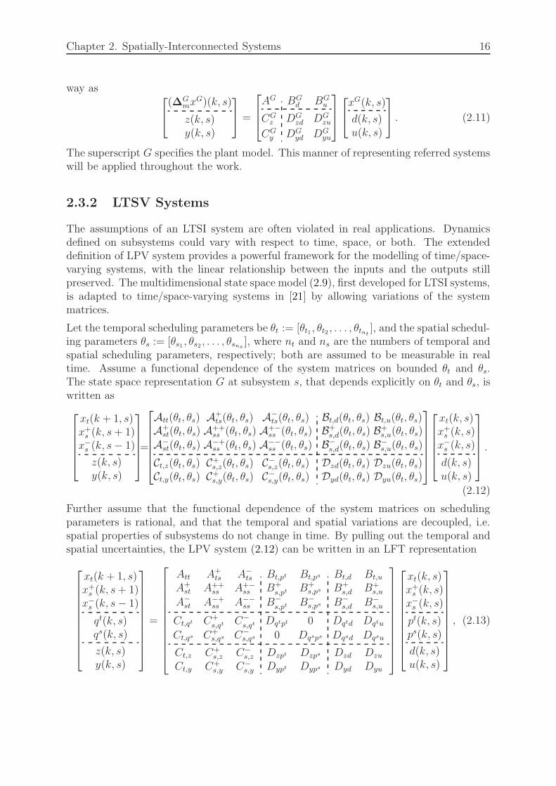
Chapter 2. Spatially-Interconnected Systems 18
It can be recovered from (2.16) and (2.17) by applying the upper LFT definition (seeAppendix C.1)
AG(Θt,Θs) BGd (Θt,Θs) BG
u (Θt,Θs)
CGz (Θt,Θs) DG
zd(Θt,Θs) DGzu(Θt,Θs)
CGy (Θt,Θs) DG
yd(Θt,Θs) DGyu(Θt,Θs)
=
AG BGd BG
u
CGz DG
zd DGzu
CGy DG
yd DGyu
+
BGp
DGzp
DGyp
ΥG(I −DG
qpΥG)[CG
q DGqd DG
qu
]. (2.19)
2.4 Controller Structure
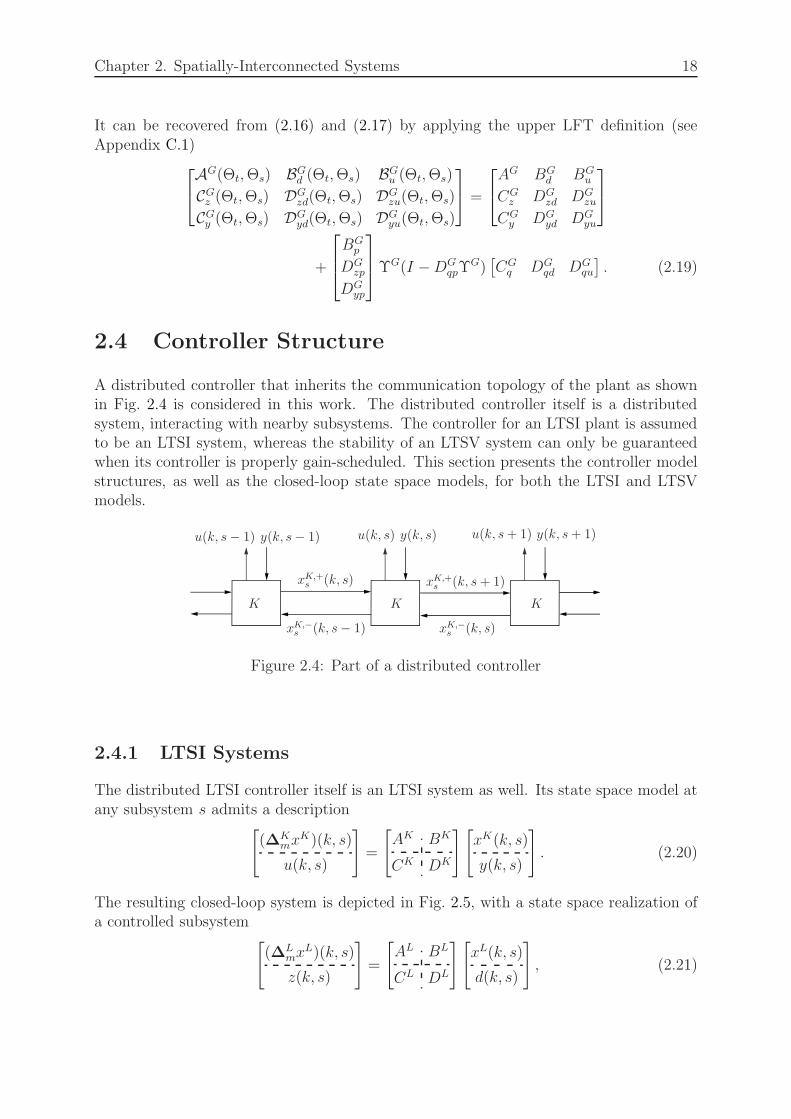
A distributed controller that inherits the communication topology of the plant as shownin Fig. 2.4 is considered in this work. The distributed controller itself is a distributedsystem, interacting with nearby subsystems. The controller for an LTSI plant is assumedto be an LTSI system, whereas the stability of an LTSV system can only be guaranteedwhen its controller is properly gain-scheduled. This section presents the controller modelstructures, as well as the closed-loop state space models, for both the LTSI and LTSVmodels.
K KK
xK,+s (k, s) xK,+
s (k, s+ 1)
xK,−s (k, s− 1) xK,−
s (k, s)
u(k, s− 1) y(k, s− 1) u(k, s) y(k, s) u(k, s+ 1) y(k, s+ 1)
Figure 2.4: Part of a distributed controller
2.4.1 LTSI Systems
The distributed LTSI controller itself is an LTSI system as well. Its state space model atany subsystem s admits a description
[
(∆Kmx
K)(k, s)
u(k, s)
]
=
[
AK BK
CK DK
][
xK(k, s)
y(k, s)
]
. (2.20)
The resulting closed-loop system is depicted in Fig. 2.5, with a state space realization ofa controlled subsystem
[
(∆Lmx
L)(k, s)
z(k, s)
]
=
[
AL BL
CL DL
][
xL(k, s)
d(k, s)
]
, (2.21)
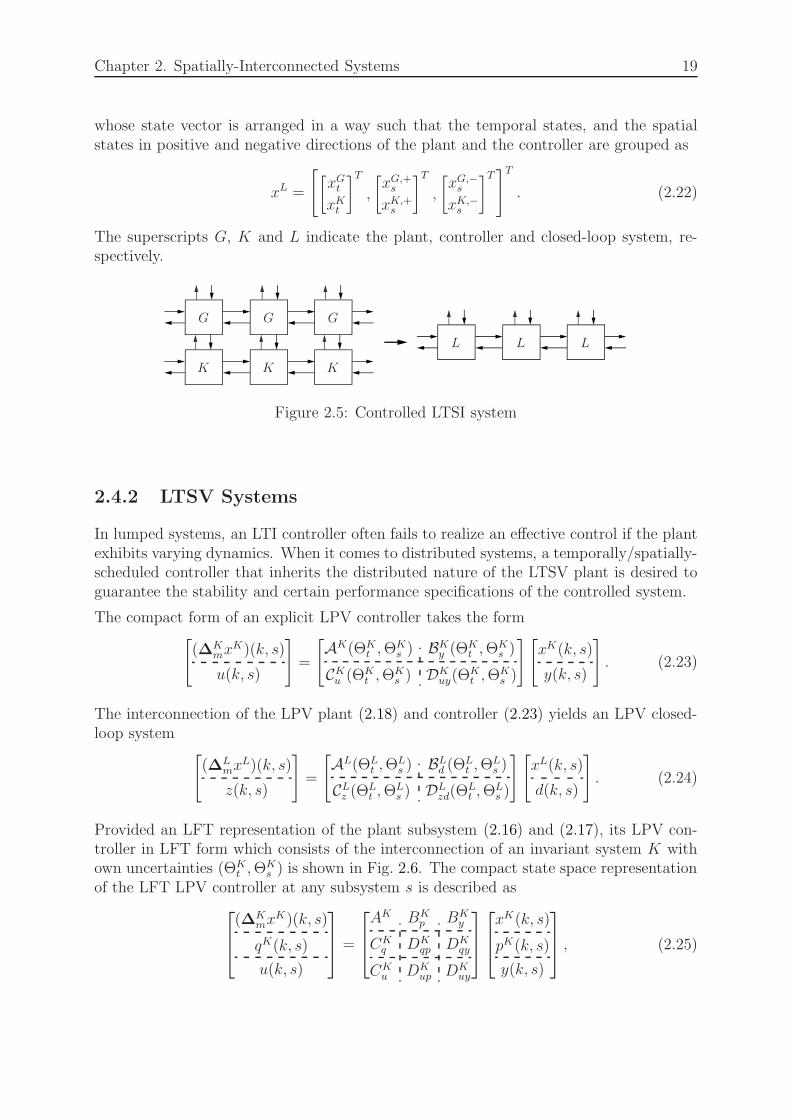
Chapter 2. Spatially-Interconnected Systems 19
whose state vector is arranged in a way such that the temporal states, and the spatialstates in positive and negative directions of the plant and the controller are grouped as
xL =
[[xGt
xKt
]T
,
[xG,+s
xK,+s
]T
,
[xG,−s
xK,−s
]T]T
. (2.22)
The superscripts G, K and L indicate the plant, controller and closed-loop system, re-spectively.
GGG
KKK
LLL
Figure 2.5: Controlled LTSI system
2.4.2 LTSV Systems
In lumped systems, an LTI controller often fails to realize an effective control if the plantexhibits varying dynamics. When it comes to distributed systems, a temporally/spatially-scheduled controller that inherits the distributed nature of the LTSV plant is desired toguarantee the stability and certain performance specifications of the controlled system.
The compact form of an explicit LPV controller takes the form[
(∆Kmx
K)(k, s)
u(k, s)
]
=
[
AK(ΘKt ,Θ
Ks ) BK
y (ΘKt ,Θ
Ks )
CKu (ΘK
t ,ΘKs ) DK
uy(ΘKt ,Θ
Ks )
][
xK(k, s)
y(k, s)
]
. (2.23)
The interconnection of the LPV plant (2.18) and controller (2.23) yields an LPV closed-loop system
[
(∆Lmx
L)(k, s)
z(k, s)
]
=
[
AL(ΘLt ,Θ
Ls ) BL
d (ΘLt ,Θ
Ls )
CLz (Θ
Lt ,Θ
Ls ) DL
zd(ΘLt ,Θ
Ls )
][
xL(k, s)
d(k, s)
]
. (2.24)
Provided an LFT representation of the plant subsystem (2.16) and (2.17), its LPV con-troller in LFT form which consists of the interconnection of an invariant system K withown uncertainties (ΘK
t ,ΘKs ) is shown in Fig. 2.6. The compact state space representation
of the LFT LPV controller at any subsystem s is described as
(∆Kmx
K)(k, s)
qK(k, s)
u(k, s)
=
AK BKp BK
y
CKq DK
qp DKqy
CKu DK
up DKuy
xK(k, s)
pK(k, s)
y(k, s)
, (2.25)

Chapter 2. Spatially-Interconnected Systems 20
whose uncertainty channel pK(k, s) =
[pt,K(k, s)ps,K(k, s)
]
, qK(k, s) =
[qt,K(k, s)qs,K(k, s)
]
, and
pK =
[ΘK
t
ΘKs
]
qK := ΥKqK . (2.26)
GGG
KKK
Θt
Θs−1
Θt
Θs
Θt
Θs+1
ΘKs−1 ΘK
s ΘKs+1
ΘKtΘK
tΘKt
Figure 2.6: Interconnection between LFT plant subsystems and LFT controller subsys-tems
The interconnection between the plant subsystem (2.16) and (2.17), and the controllersubsystem (2.25) and (2.26), leads to a closed-loop distributed system in LFT form asshown in Fig. 2.7 with augmented plant and controller uncertainties, where the dynamicsof each controlled subsystem are governed by
(∆Lmx
L)(k, s)
qL(k, s)
z(k, s)
=
AL BLp BL
d
CLq DL
qp DLqd
CLz DL
zp DLzd
xL(k, s)
pL(k, s)
d(k, s)
, (2.27)
with
pL(k, s) =
[pL,t(k, s)pL,s(k, s)
]
=
pG,t(k, s)pK,t(k, s)
pG,s(k, s)pK,s(k, s)
=
Θt
ΘKt
Θs
ΘKs
qG,t(k, s)qK,t(k, s)
qG,s(k, s)qK,s(k, s)
:=
[ΘL
t
ΘLs
] [qL,t(k, s)qL,s(k, s)
]
:= ΥLqL(k, s). (2.28)
Remark :
• Under certain assumptions, the controller uncertainty can be determined as a copyof the plant uncertainty, i.e. ΥK = ΥG, at the price of conservatism. The controllerscheduling policy will be discussed in Chapter 6.

Chapter 2. Spatially-Interconnected Systems 21
LLL
Θt
ΘKt
Θs−1
ΘKs−1
Θt
ΘKt
Θs
ΘKs
Θt
ΘKt
Θs+1
ΘKs+1
Figure 2.7: Controlled LTSV distributed system in LFT representation
2.5 Well-Posedness, Stability and Performance
Well-posedness, stability and performance are three major issues addressed in systemanalysis, which apply to spatially-interconnected systems as well. In [8], the three aspectsare well defined for LTSI systems with continuous temporal and continuous spatial vari-ables. Nevertheless, the experimentally identified plant models are normally discrete inboth time and space. Meanwhile, most controllers can only be implemented digitally inpractice. Thus, provided the state space realizations in Section 2.3 and 2.4 with discretetime and space, the bilinear transformation C.3 (see Appendix C) has to be performed toconvert a discrete distributed system to its continuous counterpart, such that the analysisconditions developed in [8] can be applied. The continuous closed-loop matrices after con-version are denoted as (AL, BL, CL, DL). From here on, the overhead bars above systemmatrices indicate a continuous system; otherwise discrete.
In this section, definitions of well-posedness, exponential stability and quadratic perfor-mance in the context of spatially-distributed systems are discussed. Analysis conditionsfor an LTSI system to be exponentially stable and satisfy the desired quadratic perfor-mance are provided. Conditions for LTSV systems will be discussed in Chapter 6 whenit comes to the LPV controller design.
2.5.1 Well-Posedness
Definition 2.7 (Well-Posedness [44]) A feedback system is considered to be well-posed if all closed-loop transfer matrices are well-defined and proper. It is equivalent to:there exist unique and bounded solutions to the system equations when signals are injectedanywhere.
Well-posedness in a spatially-interconnected system implies the existence of bounded out-puts at all subsystems, given any bounded noise n+ in positive direction, n− in negativedirection and disturbance d injected in the loop as shown in Fig. 2.8.
Theorem 2.1 ([8]) A distributed system in the form of (2.21) is well-posed, if and only

Chapter 2. Spatially-Interconnected Systems 22
z(k, s− 1) d(k, s− 1) z(k, s) d(k, s) z(k, s+ 1) d(k, s+ 1)n+(k, s− 1) n+(k, s)
n−(k, s) n−(k, s+ 1)
LLL
Figure 2.8: Distributed system with noise and disturbance injected
if (∆Ls,m − AL
ss) is invertible on space l2, where ∆Ls,m and AL
ss are defined as
∆Ls,m :=
[
SImL+
S−1ImL−
]
, ALss :=
[AL,++
ss AL,+−ss
AL,−+ss AL,−−
ss
]
, (2.29)
respectively.
2.5.2 Exponential Stability and Quadratic Performance
Consider again the controlled system (2.21). Definitions of exponential stability, quadraticperformance and structured Lyapunov functions in the context of distributed systems,as well as conditions for an LTSI system to be exponential stable and fulfil quadraticperformance, are given below.
Definition 2.8 (Exponential Stability) The discrete system (2.21) is said to be ex-ponentially stable if there exist positive α and β such that
‖ An ‖l2≤ αe−βn, (2.30)
where the operator A is defined [8] as A := ALtt +
[
AL,+ts AL,−
ts
](∆L
s,m − ALss)
−1
[
AL,+st
AL,−st
]
;
n is a positive integer.
Readers are referred to [8] regarding the stability condition for continuous systems. Con-dition (2.30) for discrete systems follows immediately.
Definition 2.9 (Quadratic Performance) A stable closed-loop system (2.21) is saidto have quadratic performance γ, if the induced L2 norm that maps d ∈ L2 to z ∈ L2 isbounded by γ > 0, i.e. ‖ z ‖L2
< γ ‖ d ‖L2, which can be expressed in an integral quadratic
form∞∑
k=1
∞∑
s=−∞
[∗]T[−γI 0
0 1γI
] [d(k, s)z(k, s)
]T
≤ 0. (2.31)
When γ < 1, the system is said to be contractive.
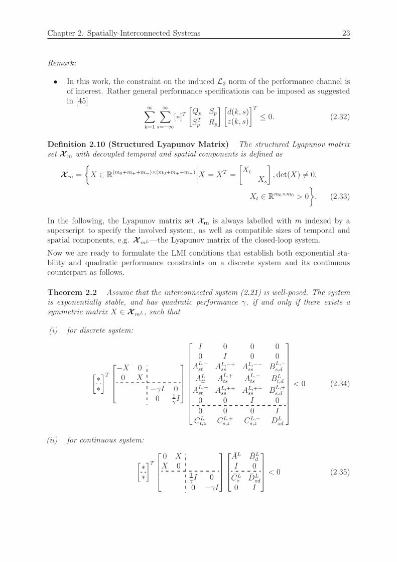
Chapter 2. Spatially-Interconnected Systems 23
Remark :
• In this work, the constraint on the induced L2 norm of the performance channel isof interest. Rather general performance specifications can be imposed as suggestedin [45]
∞∑
k=1
∞∑
s=−∞
[∗]T[Qp Sp
STp Rp
] [d(k, s)z(k, s)
]T
≤ 0. (2.32)
Definition 2.10 (Structured Lyapunov Matrix) The structured Lyapunov matrixset Xm with decoupled temporal and spatial components is defined as
Xm =
X ∈ R(m0+m++m−)×(m0+m++m−)
∣∣∣∣X = XT =
[Xt
Xs
]
, det(X) 6= 0,
Xt ∈ Rm0×m0 > 0
. (2.33)
In the following, the Lyapunov matrix set Xm is always labelled with m indexed by asuperscript to specify the involved system, as well as compatible sizes of temporal andspatial components, e.g. XmL—the Lyapunov matrix of the closed-loop system.
Now we are ready to formulate the LMI conditions that establish both exponential sta-bility and quadratic performance constraints on a discrete system and its continuouscounterpart as follows.
Theorem 2.2 Assume that the interconnected system (2.21) is well-posed. The systemis exponentially stable, and has quadratic performance γ, if and only if there exists asymmetric matrix X ∈ XmL, such that
(i) for discrete system:
[∗∗
]T
−X 00 X
−γI 00 1
γI
I 0 0 00 I 0 0
AL,−st AL,−+
ss AL,−−ss BL,−
s,d
ALtt AL,+
ts AL,−ts BL
t,d
AL,+st AL,++
ss AL,+−ss BL,+
s,d
0 0 I 0
0 0 0 ICL
t,z CL,+s,z CL,−
s,z DLzd
< 0 (2.34)
(ii) for continuous system:
[∗∗
]T
0 XX 0
1γI 0
0 −γI
AL BLd
I 0
CLz DL
zd
0 I
< 0 (2.35)
Chapter 2. Spatially-Interconnected Systems 24
Proof The proof of condition (2.34) is a simplified version of the one in [21], where an LMIcondition that establishes exponential stability and quadratic performance of an LTSVsystem is derived. The proof of (2.35) is provided in [8].
2.6 Summary
This introductory chapter has summarized some important definitions and results in theanalysis of spatially-distributed systems. Definitions of signal and system norms in thecontext of multidimensional systems have been presented. An interconnected-systemframework considered throughout this thesis has been introduced, where the distributedsystem is treated as the interconnection of an array of virtually-divided subsystems. Amultidimensional state space model that defines the dynamics on subsystems has beenprovided both for parameter-invariant and -varying models. It is desired in a distributedcontrol system, that the controller inherits the spatial structure of the plant. The dis-tributed controllers for both LTSI and LTSV plants have been discussed. Definitionsof well-posedness, stability and performance for spatially-distributed systems have beengiven, as well as the LMI conditions that establish the exponential stability and quadraticperformance of an LTSI system.
Chapter 3
Physical Modelling
3.1 Introduction
Experimental structures similar to the one constructed – a long beam equipped witha large array of distributed actuators and sensors – to the best of the author’s knowl-edge, have not been reported yet. Due to the lack of prior knowledge and experience,understanding the physical laws of both the flexible beam structure and attached actua-tor/sensor pairs individually and altogether provides important insights into the systembehaviour. This chapter deals with the physical modelling of the 4.8 m long actuatedaluminium beam.
Dynamics of multidimensional systems are often governed by PDEs—functions of multi-variables and their partial derivatives. The governing PDEs of many continuum physicsare available, e.g. the heat equation for the distribution of heat, Euler-Bernoulli equationfor the vibration of beam-like structures, etc. Exact analytic solutions to complex PDEsmay be difficult or even not possible to obtain. For this reason, numerical approachesare often applied to calculate approximated solutions. Three conventional techniquesfor solving PDEs numerically are: the finite difference (FD) method, the finite volumemethod and the FE method. One common feature of the three techniques is that PDEsare solved at discretized spatial locations—a finite approximation to the set of infinitecontinuous solutions. The approximated solution converges to the exact solution of aPDE, as the number of elements is increased.
Without prior knowledge of the governing PDE of the experimental structure, a piezo-electric FE approach that accounts for the distributed piezoelectric sensors and actuatorsis applied in this chapter to model the coupled electric and elastic behaviour, with boththe aluminium beam and the attached piezo patches modelled based on one-dimensionEuler-Bernoulli beam theory. The theoretical FE model is first obtained from known andassumed physical properties, yet it does not suffice for an accurate representation of thetest structure, owing to the complexity of the structure. An essential step is to apply theexperimental modal analysis to update the FE model using measurements, such that thediscrepancy between the test structure and the obtained FE model is minimized.
25

Chapter 3. Physical Modelling 26
The remainder of this chapter is organized as follows: Section 3.2 gives a short intro-duction to the direct and inverse piezoelectric effect, as well as the linear constitutiveequations when a piezo patch functions as actuator and as sensor, respectively. Section3.3 presents first the physical profiles of the piezo patches employed in this work. UnderEuler-Bernoulli beam theory, the linear dynamics of a piezo patch as actuator and assensor are illustrated in Section 3.3.2 and Section 3.3.3, respectively. In Section 3.4, apiezoelectric FE modelling approach [23] is applied to model the test structure in termsof its mass and stiffness matrices, based on given or assumed physical parameters. Theobtained theoretical FE model is updated with the implementation of the experimentalmodal analysis in Section 3.5.
3.2 Piezoelectric Effect
Piezoelectric material possesses the ability to convert between mechanical and electricalenergies. The conversion is a reversible process in materials that exhibit both the directpiezoelectric effect and the inverse piezoelectric effect. The direct piezoelectric effect– a phenomenon that certain crystalline materials generate an electric charge when anexternal force is applied – was first demonstrated by the brothers Pierre Curie and JacquesCurie in 1880 [46]. The inverse piezoelectric effect induces a deformation of the materialwith the application of an electric field parallel to the direction of polarization.
The most commonly used piezoelectric materials are Lead Zirconate Titanate (PZT) andPolyvinylidene Difluorid (PVDF) [47]. PZT is a ceramic material, composed of negativeand positive ions. Each pair of positive and negative ions can be visualized as an electricdipole. Before poling, the dipoles are oriented randomly with the crystal exhibiting nopiezoelectric effect. During poling, a strong electric field is applied to the material to forceall dipoles to line up in nearly the same direction. After removing the electric field, thepolarisation remains in the material, giving rise to the piezoelectricity. PZT materials arewidely used as both actuators and sensors. Unlike the crystal structure of PZT, the othercommonly used material PVDF is a polymer of molecule chains CH2−CF2. Depending onthe poled direction, the positive hydrogen atoms are attracted to the negative side of theelectric field, whereas the negative fluorine atoms are attracted to the positive side. PVDFis mainly used as sensor due to its high piezo-, pyro-, and ferroelectric properties [48]. Inthis work, piezoelectric components made of PZT materials are exclusively employed.
Constitutive Equations
Due to the presence of ferro-electricity, pyroelectricity or aging, piezoelectric materialsmay exhibit strong nonlinearities and hysteresis effect. Despite of that, the linear theoryis commonly used to determine the piezoelectric properties of the poled ceramic materialunder certain conditions. The notations as in the IEEE standard on piezoelectricity [49]are used here to establish the coupled electrical and mechanical constitutive equations
S = sET + dE (3.1)
D = dT + ǫTE, (3.2)
Chapter 3. Physical Modelling 27
where D denotes the electric displacement (electric charge per unit area, Coulomb/m2),E the electric field (V/m), S the strain and T the stress (N/m2). Under the linearpiezoelectricity theory, all coefficients are treated as constants: the piezoelectric constantd in (3.1) relates the electric field to the strain without the presence of mechanical stress,whereas sE denotes the compliance when the electric field is constant; ǫT in (3.2) refersto the relative permittivity of the material when constant stress is applied. Note that thesuperscripts E and T in the context of IEEE standard on piezoelectricity denote that theapplied electric field and stress are constant, respectively.
3.3 Piezoelectric Actuators/Sensors
This section introduces the physical profiles and linear dynamics of the piezo patchesused as actuators and sensors, respectively. The governing equations are derived from theconstitutive equations (3.1) and (3.2) according to the Euler-Bernoulli assumption.
3.3.1 Piezoelectric Patch Profile
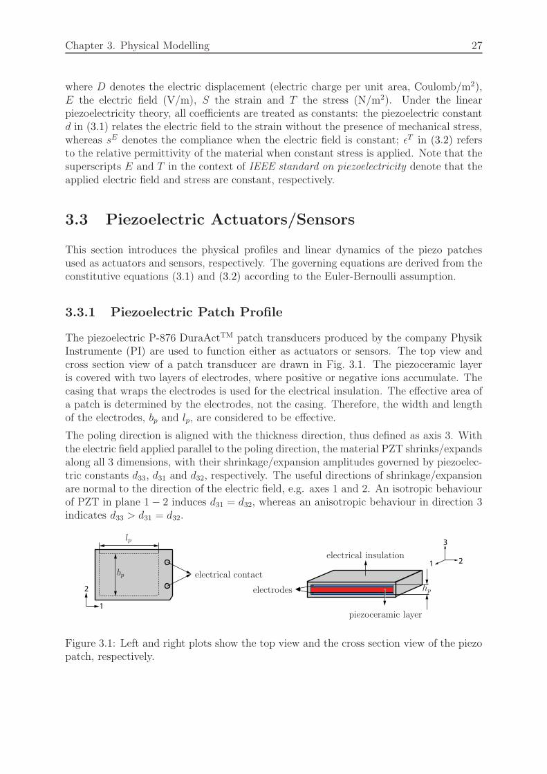
The piezoelectric P-876 DuraActTM patch transducers produced by the company PhysikInstrumente (PI) are used to function either as actuators or sensors. The top view andcross section view of a patch transducer are drawn in Fig. 3.1. The piezoceramic layeris covered with two layers of electrodes, where positive or negative ions accumulate. Thecasing that wraps the electrodes is used for the electrical insulation. The effective area ofa patch is determined by the electrodes, not the casing. Therefore, the width and lengthof the electrodes, bp and lp, are considered to be effective.
The poling direction is aligned with the thickness direction, thus defined as axis 3. Withthe electric field applied parallel to the poling direction, the material PZT shrinks/expandsalong all 3 dimensions, with their shrinkage/expansion amplitudes governed by piezoelec-tric constants d33, d31 and d32, respectively. The useful directions of shrinkage/expansionare normal to the direction of the electric field, e.g. axes 1 and 2. An isotropic behaviourof PZT in plane 1− 2 induces d31 = d32, whereas an anisotropic behaviour in direction 3indicates d33 > d31 = d32.
1
2
3
1 2
electrodes
piezoceramic layer
electrical insulation
bp
lp
electrical contact
hp
Figure 3.1: Left and right plots show the top view and the cross section view of the piezopatch, respectively.
Chapter 3. Physical Modelling 28
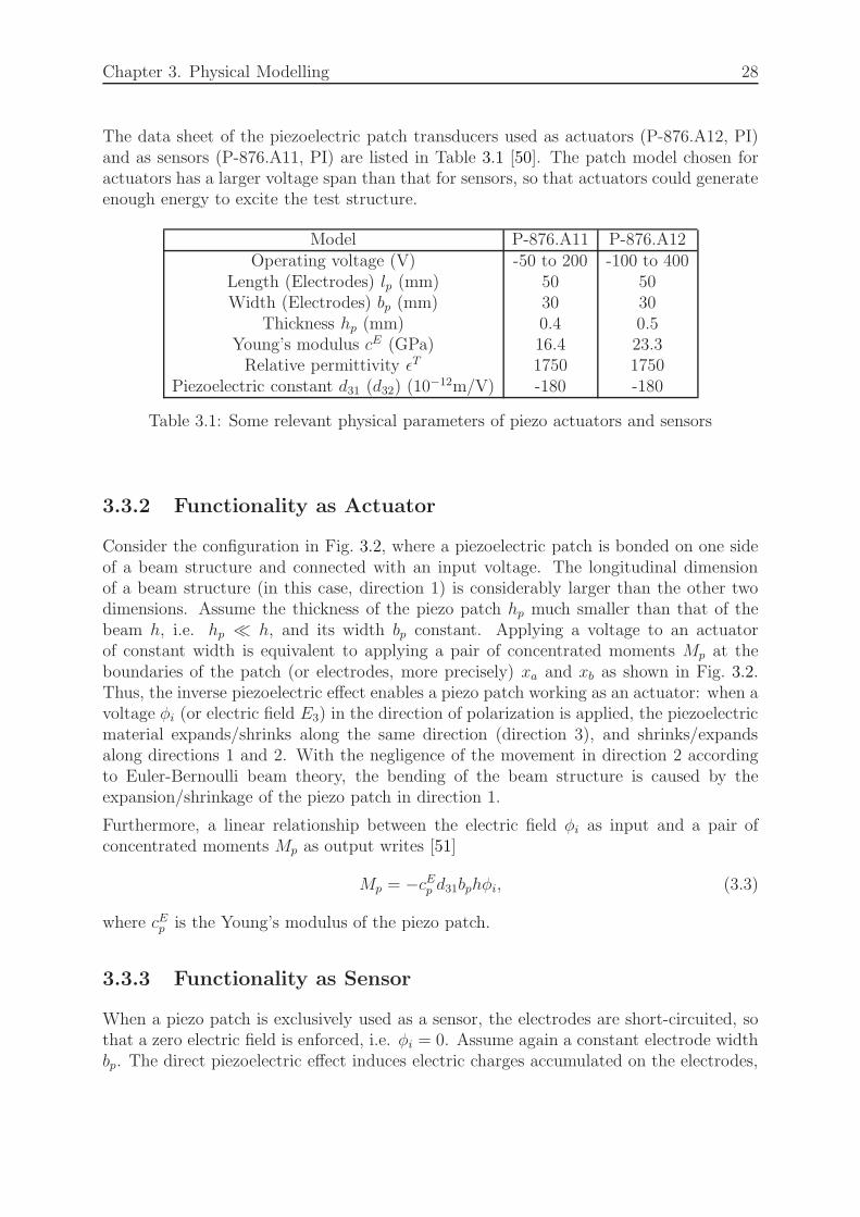
The data sheet of the piezoelectric patch transducers used as actuators (P-876.A12, PI)and as sensors (P-876.A11, PI) are listed in Table 3.1 [50]. The patch model chosen foractuators has a larger voltage span than that for sensors, so that actuators could generateenough energy to excite the test structure.
Model P-876.A11 P-876.A12Operating voltage (V) -50 to 200 -100 to 400
Length (Electrodes) lp (mm) 50 50Width (Electrodes) bp (mm) 30 30
Thickness hp (mm) 0.4 0.5Young’s modulus cE (GPa) 16.4 23.3Relative permittivity ǫT 1750 1750
Piezoelectric constant d31 (d32) (10−12m/V) -180 -180
Table 3.1: Some relevant physical parameters of piezo actuators and sensors
3.3.2 Functionality as Actuator
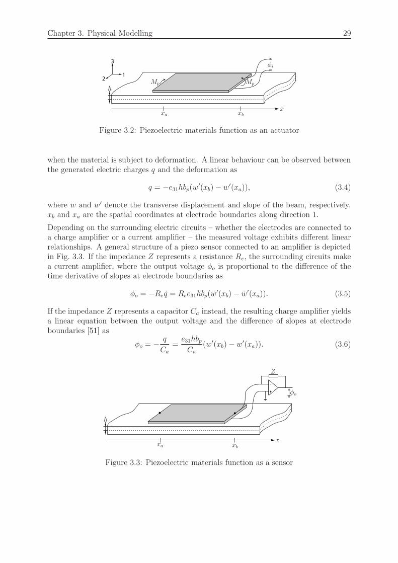
Consider the configuration in Fig. 3.2, where a piezoelectric patch is bonded on one sideof a beam structure and connected with an input voltage. The longitudinal dimensionof a beam structure (in this case, direction 1) is considerably larger than the other twodimensions. Assume the thickness of the piezo patch hp much smaller than that of thebeam h, i.e. hp ≪ h, and its width bp constant. Applying a voltage to an actuatorof constant width is equivalent to applying a pair of concentrated moments Mp at theboundaries of the patch (or electrodes, more precisely) xa and xb as shown in Fig. 3.2.Thus, the inverse piezoelectric effect enables a piezo patch working as an actuator: when avoltage φi (or electric field E3) in the direction of polarization is applied, the piezoelectricmaterial expands/shrinks along the same direction (direction 3), and shrinks/expandsalong directions 1 and 2. With the negligence of the movement in direction 2 accordingto Euler-Bernoulli beam theory, the bending of the beam structure is caused by theexpansion/shrinkage of the piezo patch in direction 1.
Furthermore, a linear relationship between the electric field φi as input and a pair ofconcentrated moments Mp as output writes [51]
Mp = −cEp d31bphφi, (3.3)
where cEp is the Young’s modulus of the piezo patch.
3.3.3 Functionality as Sensor
When a piezo patch is exclusively used as a sensor, the electrodes are short-circuited, sothat a zero electric field is enforced, i.e. φi = 0. Assume again a constant electrode widthbp. The direct piezoelectric effect induces electric charges accumulated on the electrodes,
Chapter 3. Physical Modelling 29
3
21
MpMp
h
φi
xa xbx
Figure 3.2: Piezoelectric materials function as an actuator
when the material is subject to deformation. A linear behaviour can be observed betweenthe generated electric charges q and the deformation as
q = −e31hbp(w′(xb)− w′(xa)), (3.4)
where w and w′ denote the transverse displacement and slope of the beam, respectively.xb and xa are the spatial coordinates at electrode boundaries along direction 1.
Depending on the surrounding electric circuits – whether the electrodes are connected toa charge amplifier or a current amplifier – the measured voltage exhibits different linearrelationships. A general structure of a piezo sensor connected to an amplifier is depictedin Fig. 3.3. If the impedance Z represents a resistance Re, the surrounding circuits makea current amplifier, where the output voltage φo is proportional to the difference of thetime derivative of slopes at electrode boundaries as
φo = −Req = Ree31hbp(w′(xb)− w′(xa)). (3.5)
If the impedance Z represents a capacitor Ca instead, the resulting charge amplifier yieldsa linear equation between the output voltage and the difference of slopes at electrodeboundaries [51] as
φo = − q
Ca
=e31hbpCa
(w′(xb)− w′(xa)). (3.6)
h
Z
φo
xa xb
x
Figure 3.3: Piezoelectric materials function as a sensor
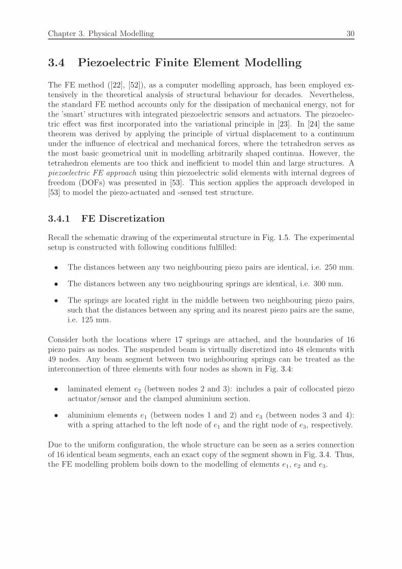
Chapter 3. Physical Modelling 30
3.4 Piezoelectric Finite Element Modelling
The FE method ([22], [52]), as a computer modelling approach, has been employed ex-tensively in the theoretical analysis of structural behaviour for decades. Nevertheless,the standard FE method accounts only for the dissipation of mechanical energy, not forthe ’smart’ structures with integrated piezoelectric sensors and actuators. The piezoelec-tric effect was first incorporated into the variational principle in [23]. In [24] the sametheorem was derived by applying the principle of virtual displacement to a continuumunder the influence of electrical and mechanical forces, where the tetrahedron serves asthe most basic geometrical unit in modelling arbitrarily shaped continua. However, thetetrahedron elements are too thick and inefficient to model thin and large structures. Apiezoelectric FE approach using thin piezoelectric solid elements with internal degrees offreedom (DOFs) was presented in [53]. This section applies the approach developed in[53] to model the piezo-actuated and -sensed test structure.
3.4.1 FE Discretization
Recall the schematic drawing of the experimental structure in Fig. 1.5. The experimentalsetup is constructed with following conditions fulfilled:
• The distances between any two neighbouring piezo pairs are identical, i.e. 250 mm.
• The distances between any two neighbouring springs are identical, i.e. 300 mm.
• The springs are located right in the middle between two neighbouring piezo pairs,such that the distances between any spring and its nearest piezo pairs are the same,i.e. 125 mm.
Consider both the locations where 17 springs are attached, and the boundaries of 16piezo pairs as nodes. The suspended beam is virtually discretized into 48 elements with49 nodes. Any beam segment between two neighbouring springs can be treated as theinterconnection of three elements with four nodes as shown in Fig. 3.4:
• laminated element e2 (between nodes 2 and 3): includes a pair of collocated piezoactuator/sensor and the clamped aluminium section.
• aluminium elements e1 (between nodes 1 and 2) and e3 (between nodes 3 and 4):with a spring attached to the left node of e1 and the right node of e3, respectively.
Due to the uniform configuration, the whole structure can be seen as a series connectionof 16 identical beam segments, each an exact copy of the segment shown in Fig. 3.4. Thus,the FE modelling problem boils down to the modelling of elements e1, e2 and e3.

Chapter 3. Physical Modelling 31
e1 e2 e3
1 2 3 4
x1 x2 x3 x4
Figure 3.4: Beam segment between two neighbouring springs comprised of three elements
3.4.2 Modelling Based on Euler-Bernoulli Beam Theory
It has been suggested in [54] that beam theory is not accurate enough to model systemswith collocated actuators and sensors due to the fact that the one-dimensional beamtheory considers only the bending moment at elemental nodes, and neglects the torsionalmovement. Instead, shell theory has been proven to be a more suitable technique to modelsuch a system. Nevertheless, recall the physical parameters of the structure: the lengthof the beam (4.8 m) is significantly larger than its width (40 mm) and thickness (3 mm);that implies a representative beam structure, whose transverse displacements dominatethe vibratory dynamics. Thus, the one-dimensional beam theory could be appropriate forthe FE modelling of the concerned structure here. Its validity will be examined in Section3.5.
The simplest Euler-Bernoulli beam theory [55] assumes two DOFs at each node: thetransverse displacement w and its slope w′ = dw
dx, where axis x is along the longitudinal
direction. An element of two nodes has four DOFs as shown in Fig. 3.5 (a). A vector ue
that collects the nodal displacements at nodes 1 and 2 is denoted as
ue =[w1 w′
1 w2 w′2
]T. (3.7)
Meanwhile, external loads could act on nodes in form of transverse force f and bendingmoment M as shown in Fig. 3.5 (b), denoted as
pe =[f1 M1 f2 M2
]T. (3.8)
M1
f2f1
M2
w1 w2
w′1 w′
2
11 22
(a) (b)
Figure 3.5: Under Euler-Bernoulli beam theory, each node has 2 DOFs: transverse dis-placement and slope (a); external loads act on each node in two forms: transverse forceand moment (b).

Chapter 3. Physical Modelling 32
The FE modelling of the given structure is realized in the following three steps.
Elemental Formulation of Elements e1 and e3
The FE formulations of elements e1 and e3 follow the classical FE modelling routine [22]that accounts for only the mechanical energy. Provided the nodal displacements ue (inthis case, ue1 and ue3), the transverse displacement at any continuous location over theelement, w(x), with x1 ≤ x ≤ x2 for element e1, and x3 ≤ x ≤ x4 for element e3, can bedetermined through interpolation using a set of pre-chosen shape functions as
w(x) = Nu(x)ue =
[
Nw1u N
w′
1u Nw2
u Nw′
2u
]
w1
w′1
w2
w′2
(3.9)
where Nu(x), or Nu for notational simplicity, denotes the shape functions, and meets theC1 continuity requirement. The C1 continuity is required, because both the transversedisplacement w and its spatial derivative w′ need to be continuous over the element.The shape functions often employed for the modelling of a beam element in terms of thedimensionless coordinate ξ (−1 ≤ ξ ≤ 1) are
Nw1
u =1
4(1− ξ)2(2 + ξ) (3.10)
Nw′
1u =
1
8le(1− ξ)2(1 + ξ) (3.11)
Nw2
u =1
4(1 + ξ)2(2− ξ) (3.12)
Nw′
2u = −1
8le(1 + ξ)2(1− ξ), (3.13)
where le denotes the length of the beam element. The four shape functions are shown inFig. 3.6.
The FE modelling treats each element as a spring-mass-damper system. The governingequation of element e1 or e3 takes the form
Meue + Ceue +Keuuu
e = pe, (3.14)
where e = e1 or e = e3. The elemental displacements ue and external loads pe are definedin the same way as (3.7) and (3.8), respectively. The elemental mass matrix Me andstiffness matrix Ke
uu are derived from the variational principle [52] as:
Me =
∫
V eb
ρbNTu NudV
eb (3.15)
Keuu =
∫
V eb
BTu c
Eb BudV
eb , (3.16)
where Bu is the spatial derivative of shape functions Nu, i.e.
Bu = N ′u.

Chapter 3. Physical Modelling 33
0
0.5
1
0
0.02
0.04
−1 −0.5 0 0.5 10
0.5
1
−1 −0.5 0 0.5 1
−0.04
−0.02
0
Nw
1u
Nw
′ 1u
Nw
2u
Nw
′ 2u
ξξ
Figure 3.6: Shape functions used for the modelling of a beam element
The density, Young’s modulus under constant electric field and volume of the aluminiumbeam element e1 or e3 are denoted by ρb, c
Eb , and V e
b , respectively. Assume the identicalspring stiffness ks at both elements. The stiffness matrix Ke
uu computed in (3.16) ismodified for e1 and e3 as
Ke1uu(1, 1) = Ke1
uu(1, 1) + ks (3.17)
Ke3uu(3, 3) = Ke1
uu(3, 3) + ks, (3.18)
respectively, due to the fact that the left node of e1 and the right node of e3 are attachedto springs. The modelling of the damping matrix Ce will be elaborately discussed inSection 3.5.
Elemental Formulation of Element e2
The modelling of element e2 involves the mechanical and piezoelectric energy transfor-mation. As discussed in Section 3.3.2, the application of an input voltage φe
i to a piezoactuator is equivalent to the application of a pair of concentrated torques at the electrodeboundaries. Thus both the external loads pe and the actuator can generate a mechanicalmotion of the element e2. Skipping the derivation procedures [53], the governing equationthat accounts for the conversion from electrical to mechanical energy at element e2 writes
Meue + Ceue +Keuuu
e = pe −Keuφφ
ei , (3.19)
where the coupling stiffness matrix Keuφ relates the mechanical and electrical variables in
piezo actuators.
On the other side, due to the direct piezoelectric effect, the mechanical deformation ue
induces electrical charges qe on the electrodes of piezo sensors. The linear dynamicspresented in Section 3.3.3 yields the sensor equation
qe = Keφuu
e, (3.20)

Chapter 3. Physical Modelling 34
where the coupling stiffness matrix Keφu relates the mechanical and electrical variables in
piezo sensors.
Under the assumption that the electric potential is constant over a piezo patch, only oneelectrical DOF per patch is defined. More intuitively, φe
i and qe ∈ R at any element. Acharge amplifier is connected to the sensor electrodes to convert the generated electricalcharges to voltage as (3.6). The output equation (3.20) is modified to
φeo = −
Keφu
Ca
ue. (3.21)
The elemental mass matrix Me and stiffness matrix Keuu are constructed accounting for
the collective contributions from the actuator, the sensor and the clamped aluminiumbeam section as
Me =
∫
Va
ρaNTu NudVa +
∫
Vs
ρsNTu NudVs +
∫
V eb
ρbNTu NudV
eb (3.22)
Keuu =
∫
Va
BTu c
Ea BudVa +
∫
Vs
BTu c
Es BudVs +
∫
V eb
BTu c
Eb BudV
eb . (3.23)
The shape functions and their derivatives Nu and Bu are defined in the same way as theFE modelling of elements e1 and e3. The density, Young’s modulus under constant electricfield and volume of the actuator and the sensor are denoted by ρa, ρs, c
Ea , c
Es , Va and Vs,
respectively, where the subscript a indicates the actuator, s the sensor parameters.
Consider (3.19) as the actuator equation, and (3.21) as the sensor equation. The elementalcoupling matrices Ke
uφ and Keφu are computed as
Keuφ =
∫
Va
BTu e
TaBφadVa (3.24)
Keφu =
∫
Vs
BTφse
Ts BudVs. (3.25)
The piezoelectric coupling coefficients eTa and eTs under constant stress are related to theYoung’s modulus under constant electric field by eTa = d31c
Ea and eTs = d31c
Es , respectively.
It has been justified in [54] that, the constant electric potential over element e2 yieldsBφa = 1/hpa and Bφs = 1/hps, where hpa and hps are the thicknesses of the piezo actuatorand sensor, respectively.
Globalization
After the elemental formulation of the three fundamental elements in Fig. 3.4, the globalFE model can be subsequently constructed by assembling the contribution from eachelement. The resulting global actuator and sensor equations are given by
MU + CU +KUUU = P −KUΦΦi (3.26)
Φo = −KΦUU
Ca
, (3.27)

Chapter 3. Physical Modelling 35
where U ∈ R98, Φi ∈ R16 and Φo ∈ R16 are the global mechanical variables, input andoutput voltage, respectively. Matrices M, KUU , KUΦ, KΦU and C are the global versionsof their elemental counterparts.
Consider now a self-actuating and -sensing ’smart’ system, i.e. P = 0. The actuatorequation (3.26) is rewritten as
MU + CU +KUUU = −KUΦΦi. (3.28)
Remarks :
Recall the single actuator equation (3.3) and sensor equation (3.6). To relate (3.3) to(3.28), and (3.6) to (3.27), the 3-element beam segment in Fig. 3.4 is taken as an exampleto avoid the demonstration of vectors of large sizes.
• With the application of an input voltage φe2i to the actuator of element e2, a pair
of moments Me2p are generated at nodes 2 and 3. The linear dynamics (3.3) can be
rewritten for simplicity as Me2p = gaφ
e2i , where ga is the simplified actuator constant.
The computation of the coupling matrix KUΦ in (3.28) requires the computationof the actuator constant ga, and mapping the generated moments to the correctpositions in vector KUΦΦ, i.e.
−KUΦΦ =
[. . . 0 0
︸︷︷︸
node 1
0 gaφe2i
︸ ︷︷ ︸
node 2
0 −gaφe2i
︸ ︷︷ ︸
node 3
0 0︸︷︷︸
node 4
. . .]T
(3.29)
=
[. . . 0 0
︸︷︷︸
node 1
0 Me2p
︸ ︷︷ ︸
node 2
0 −Me2p
︸ ︷︷ ︸
node 3
0 0︸︷︷︸
node 4
. . .]
.T (3.30)
Note that according to beam theory, nodes are in general subject to external loadsin the form of transverse force and bending moment. On nodes 1 and 4 there areno external loads applied, whereas the piezo actuator induces zero transverse forceand non-zero bending moments on nodes 2 and 3.
• Accoring to (3.6), output voltage φe2o is proportional to the slope difference at two
electrode boundaries. i.e. φe2o = gs(w
′(3)− w′(2)), where gs is the simplified sensorconstant. Analogously, the term KΦU
Cain (3.27) picks the slopes at nodes 2 and 3
from the mechanical variable U , computing their difference as
Φo =
[. . . gs(w
′(3)− w′(2))︸ ︷︷ ︸
sensor e2
. . .]T
=
[. . . φe2
o︸︷︷︸
sensor e2
. . .]T
. (3.31)
3.5 Updating the FE Model Using the Experimental
Modal Analysis
Although the FE model – in form of mass matrix, stiffness matrix, and two electrome-chanical coupling matrices – has been constructed based on given or assumed physical
Chapter 3. Physical Modelling 36
properties, it is unrealistic to expect that such a theoretical model accurately representsthe dynamic behaviour of the test structure, owing to the presence of damping and uncer-tain nonlinearity of the structure. To reduce the discrepancy in between, experiments needto be designed and performed to extract modal information out of measurements. Thisprocess is called experimental modal analysis, which normally consists of three phases:test preparation, frequency response measurements, and modal parameter identification[56]. To measure a frequency response, an excitation is performed at one location onthe structure, while the vibration response is measured at the same or another location.The dynamic relationship from excitation to response in frequency domain is known asFRF. A set of FRFs at all possible excitation and response locations constitutes an FRFmatrix. As an example, 16 piezo actuators and 16 piezo sensors yield an FRF matrix ofsize 16× 16.
Another important characteristic to describe the inherent structural dynamics are modes.Modes are a set of harmonic motions, and appear in an FRF as resonant peaks. Theoreti-cally, the vibratory motion of an LTI structure can be expressed as the linear combinationof an infinite number of modes. Each mode is characterized in terms of its natural fre-quency, damping factor and mode shape. Mode shapes are the displacement patternswhen the structure vibrates at its natural frequencies. The three elements together – thenatural frequency, damping factor and mode shape – are referred to as modal parametersor modal data that need to be extracted out of measured FRFs at each mode.
Updating the theoretical FE model based on identified modal parameters leads to a moreaccurate and reliable mathematical model. The updating process is realized in the fol-lowing steps.
3.5.1 Performing Experiments to Obtain FRFs
The time domain data of FRFs is usually obtained by measuring the response to a hammerimpulse or to certain excitation signals. In this work, two of the most common excitationtools - a hammer and an electromagnetic shaker - are used to produce excitation forces.The hammer produces an excitation force pulse at one selected location on the structure.A force transducer attached to the hammer tip feeds the force back to be measured. Thevibratory responses of the structure are measured by 16 attached piezo sensors simultane-ously. Instead of a wide range of frequencies, the structural behaviour at low frequenciesis of more importance in this case, since the dominant modes of the test structure aremainly located at low frequencies. Therefore, a hammer tip made of rubber is used, sothat the test structure is fully actuated at the low frequency range.
On the other hand, the electromagnetic shaker enables the excitation with various signals.The shaker is glued at one boundary (or tip) of the structure through a plastic stinger,with the applied force measured by a force transducer as shown in Fig. 3.7.
One common property using hammer or shaker excitation is the single-input and multiple-output configuration. With the actuating point fixed - either the hammer striking at oneselected location on the surface, or the shaker exciting the tip of the beam, its vibratorymotion is measured simultaneously by 16 piezo sensors. The resulting 16 measured FRFs
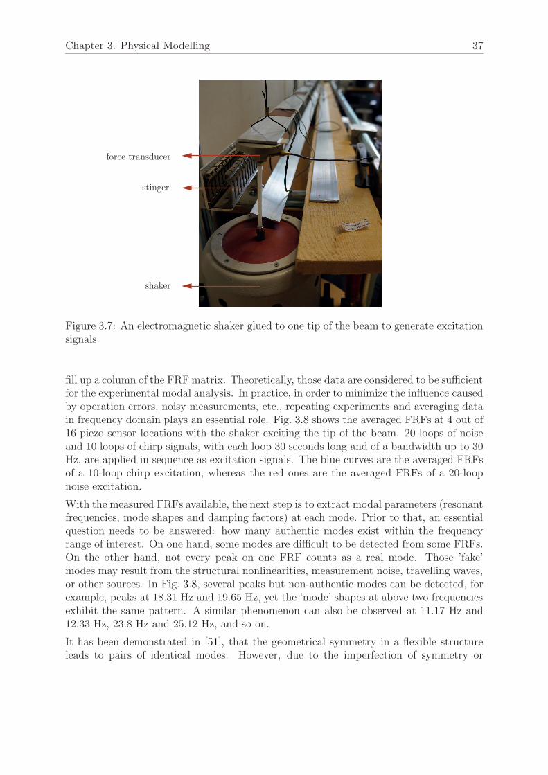
Chapter 3. Physical Modelling 37
force transducer
stinger
shaker
Figure 3.7: An electromagnetic shaker glued to one tip of the beam to generate excitationsignals
fill up a column of the FRFmatrix. Theoretically, those data are considered to be sufficientfor the experimental modal analysis. In practice, in order to minimize the influence causedby operation errors, noisy measurements, etc., repeating experiments and averaging datain frequency domain plays an essential role. Fig. 3.8 shows the averaged FRFs at 4 out of16 piezo sensor locations with the shaker exciting the tip of the beam. 20 loops of noiseand 10 loops of chirp signals, with each loop 30 seconds long and of a bandwidth up to 30Hz, are applied in sequence as excitation signals. The blue curves are the averaged FRFsof a 10-loop chirp excitation, whereas the red ones are the averaged FRFs of a 20-loopnoise excitation.
With the measured FRFs available, the next step is to extract modal parameters (resonantfrequencies, mode shapes and damping factors) at each mode. Prior to that, an essentialquestion needs to be answered: how many authentic modes exist within the frequencyrange of interest. On one hand, some modes are difficult to be detected from some FRFs.On the other hand, not every peak on one FRF counts as a real mode. Those ’fake’modes may result from the structural nonlinearities, measurement noise, travelling waves,or other sources. In Fig. 3.8, several peaks but non-authentic modes can be detected, forexample, peaks at 18.31 Hz and 19.65 Hz, yet the ’mode’ shapes at above two frequenciesexhibit the same pattern. A similar phenomenon can also be observed at 11.17 Hz and12.33 Hz, 23.8 Hz and 25.12 Hz, and so on.
It has been demonstrated in [51], that the geometrical symmetry in a flexible structureleads to pairs of identical modes. However, due to the imperfection of symmetry or

Chapter 3. Physical Modelling 38
104
0 5 10 15 20 25 30
100
102
104
100
102
104
100
102
104
100
102
frequency (Hz)
magnitude
sensor 1
sensor 5
sensor 8
sensor 16
Figure 3.8: Measured FRFs from a shaker excitation at the tip of the beam to responses at4 selected sensor locations. The blue curves are the averaged FRFs given a 10-loop chirpexcitation, whereas the red ones are the averaged FRFs given a 20-loop noise excitation.
measurement errors, those pairs of identical modes become pairs of close modes, and canbe counted only as one mode.
Taking these aspects into consideration, after the analysis of FRFs at various exciting andsensing locations, the first 10 modes below 30 Hz are finally determined, whose resonantfrequencies are
ωm = [1.221, 1.968, 3.357, 5.249, 8.362, 11.29, 15.37, 19.78, 24.17, 29.95]Hz. (3.32)
3.5.2 Updating the Mass and Stiffness Matrices
Provided known or assumed knowledge of physical properties of the structure, the FEmodel is characterised in terms of the mass and stiffness matrices as presented in Section3.4.2. Consider that the solution of the governing equation (3.28) consists of a linearcombination of mode shapes Ω, i.e. U(t) = Ωx(t), where the vector x(t) weights thecontribution of modes at time t. The characteristic equation of (3.28)
(KUU − ω2M)Ω = 0 (3.33)
1Due to the measurement noises at low frequencies, the first mode is difficult to be identified accurately.

Chapter 3. Physical Modelling 39
solves its eigenvalue problem: natural frequencies ω and mode shapes Ω. The purposeof updating the mass matrix M and the stiffness matrix KUU is formulated as: after theupdate, the computed ω and Ω from (3.33) approximate the measured natural frequenciesωm and mode shapes Ωm.
In past decades, various techniques have been developed in the structural engineeringcommunity to derive modal parameters from measured FRFs, e.g. peak picking, circlefit, global singular value decomposition (SVD) [57], and so on. The natural frequencies ofthe first 10 modes ωm (3.32) have been determined by applying the simplest peak pickingmethod, which is suitable for lightly damped systems with well-separated modes. Themode shapes Ωm are the normalized displacement of 16 sensing locations at each pickednatural frequency.
According to (3.22) and (3.23), the knowledge of structural properties determines theexactness of the computed mass and stiffness matrices. Although its geometrical dimen-sions (e.g. length, width, and thickness) are well-measurable, certain properties, like theYoung’s modulus of the beam cEb , the actuator cEa , and the sensor cEs , their densities ρb,ρa, and ρs, and the stiffness of the springs ks, though provided by the manufacturer, arehardly known accurately. This constitutes the reason for the update.
Let cEb , cEa , c
Es , ρb, ρa, ρs and ks be the parameters to be updated, and arranged as a
vector θ. The cost function is defined as
V (θ) =1
2N
∑
eT (θ)e(θ), (3.34)
withe(θ) = [ω(2)− ωm(2), ω(3)− ωm(3), . . . , ω(10)− ωm(10)]
T , (3.35)
where N is the number of selected modes, i.e. N = 9. The error vector e consists ofthe deviation between the measured natural frequencies and the ones calculated by (3.33)from 2nd to 10th modes. Note that the eigenvalue ω computed from (3.33) contains thenatural frequencies of resonant modes, as well as the frequencies of rigid body modes.The correspondence between ωm and ω in (3.35) can be detected by comparing the shapesimilarities between the computed eigenvectors Ω and measured mode shapes Ωm.
After the application of the standard Levenberg-Marquardt algorithm [58] to update theunknown parameter vector θ by minimizing the cost function (3.34), the comparisonbetween the measured and updated natural frequencies is shown in Fig. 3.9. The com-parison of mode shapes is shown in 3.10. The updated FE model demonstrates a goodapproximation to the dynamic characteristics of the test structure.
3.5.3 Updating the Damping Matrix
Unlike the mass and stiffness matrices, modelling of the damping matrix is challengingbecause the real damping model is not fully understood in the current state of the art [56][57]. However, the characterization of damping is important in terms of making accuratepredictions both in time and frequency domains. Proportional damping is a convenient
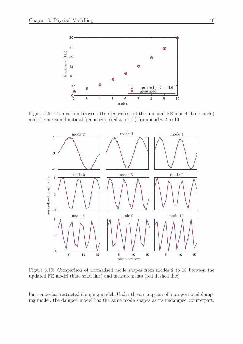
Chapter 3. Physical Modelling 40
2 3 4 5 6 7 8 9 100
5
10
15
20
25
30
updated FE modelmeasured
modes
frequency
(Hz)
Figure 3.9: Comparison between the eigenvalues of the updated FE model (blue circle)and the measured natural frequencies (red asterisk) from modes 2 to 10
−1
0
1
−1
0
1
−1
0
1
5 10 15 5 10 15 5 10 15
mode 2 mode 3 mode 4
mode 5 mode 6 mode 7
mode 8 mode 9 mode 10normalized
amplitude
piezo sensors
Figure 3.10: Comparison of normalized mode shapes from modes 2 to 10 between theupdated FE model (blue solid line) and measurements (red dashed line)
but somewhat restricted damping model. Under the assumption of a proportional damp-ing model, the damped model has the same mode shapes as its undamped counterpart,

Chapter 3. Physical Modelling 41
whereas the damped natural frequencies slightly deviate from the undamped ones whenthe structure is lightly damped. For a broader view regarding the damping identificationprocedure, readers are referred to [59] and [57]. For simplicity, a proportional viscousdamping in the form of
C = αM+ βKUU (3.36)
is assumed here, where the coefficients α and β are to be estimated after updating themass and stiffness matrices.
The Levenberg-Marquardt technique is applied again to estimate the unknown parametersα and β, such that the simulated damped FRFs approximate the measured ones. Fig. 3.11shows the comparison of the measured and simulated damped FRFs at 4 out of 16 piezosensors, with 10 loops of chirp excitations generated by the 8th piezo actuator. It can beseen that the main structural dynamics up to 30 Hz are well captured by the updatedFE model, both at resonances and anti-resonances. It can also be observed that multiplepeaks are measured at the frequencies where the FE model indicates only a single mode,e.g. near 20 and 25 Hz. It has been discussed in Section 3.5.1, that it may result from thestructural nonlinearities, imperfect geometric symmetry, interference of travelling waves,etc. To explore the physical causes of this phenomenon is out the scope of this thesis.Nevertheless, possible sources that may result in the structural asymmetry are analysedas following:
• The piezo actuator/sensor pairs may be glued in an imperfect collocated pattern.
• The springs may not be centered exactly between two neighbouring piezo pairs.
Incorporating these subtle aspects into the FE modelling would make the modelling pro-cess cumbersome and tedious. The FE model after updating is considered to representthe test structure to a satisfactory degree.
3.5.4 Compensation of the Direct Feed-Through Effect
The FRF comparisons made in Fig. 3.11 are from the excitation at the 8th actuator toresponses at non-collocated sensors. Now take a close look at the FRF from the 8thactuator to the 8th sensor as shown in Fig. 3.12 (a). It can be observed that a big gapexists between the measured and simulated FRFs over the whole frequency range, whichmay appear as a constant gain at the first sight. Actually, this discrepancy is the resultof the direct feed-through effect (or fast dynamics) from actuators to their collocatedsensors. After compensating the measurements at the 8th sensor with the fed-throughinput from its collocated actuator, i.e. y(k, 8) = y(k, 8)+ b0 ·u(k, 8), where b0 denotes thefeed-through constant, the simulation of the FE model is significantly improved as shownin Fig. 3.12 (b).
Although the existence of the direct feed-through effect within collocated piezo pairs hasbeen detected, it remains still unknown whether the feed-through constants are identicalat all 16 pairs. For this purpose, an experiment has been performed, where the 16 ac-tuators are simultaneously actuated by an identical chirp signal up to 20 Hz. Then the
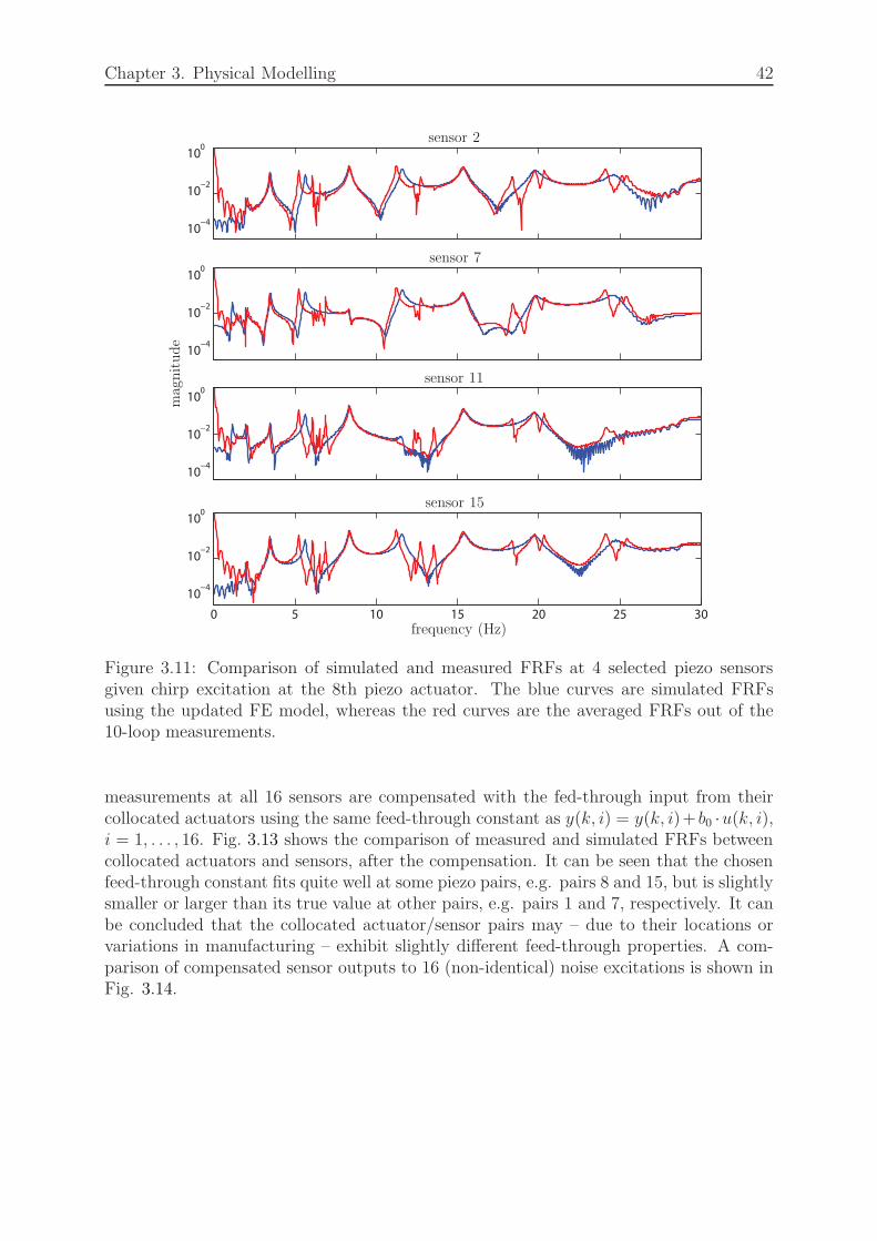
Chapter 3. Physical Modelling 42
10−4
10−2
100
10−4
10−2
100
10−4
10−2
100
0 5 10 15 20 25 30
10−4
10−2
100
sensor 2
sensor 7
sensor 11
sensor 15
frequency (Hz)
magnitude
Figure 3.11: Comparison of simulated and measured FRFs at 4 selected piezo sensorsgiven chirp excitation at the 8th piezo actuator. The blue curves are simulated FRFsusing the updated FE model, whereas the red curves are the averaged FRFs out of the10-loop measurements.
measurements at all 16 sensors are compensated with the fed-through input from theircollocated actuators using the same feed-through constant as y(k, i) = y(k, i)+ b0 ·u(k, i),i = 1, . . . , 16. Fig. 3.13 shows the comparison of measured and simulated FRFs betweencollocated actuators and sensors, after the compensation. It can be seen that the chosenfeed-through constant fits quite well at some piezo pairs, e.g. pairs 8 and 15, but is slightlysmaller or larger than its true value at other pairs, e.g. pairs 1 and 7, respectively. It canbe concluded that the collocated actuator/sensor pairs may – due to their locations orvariations in manufacturing – exhibit slightly different feed-through properties. A com-parison of compensated sensor outputs to 16 (non-identical) noise excitations is shown inFig. 3.14.
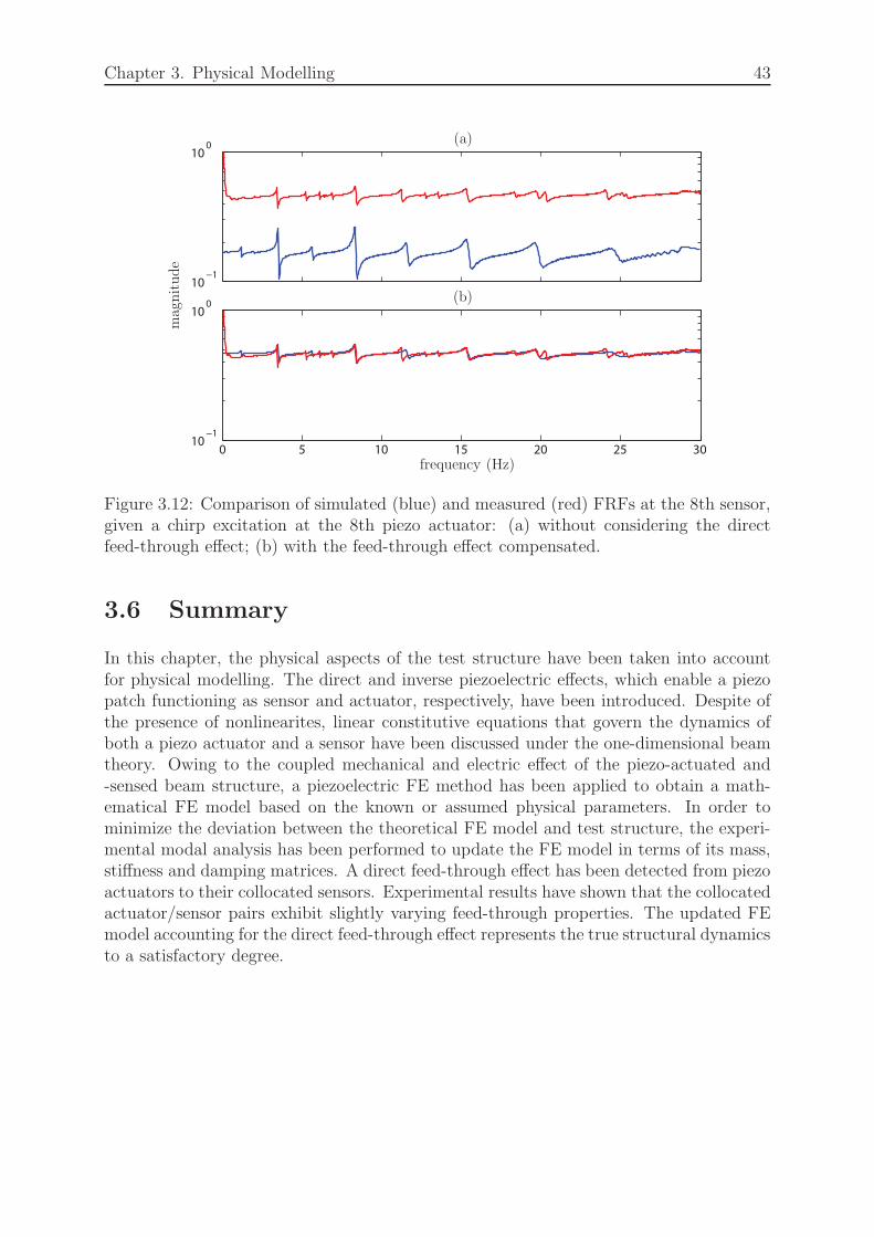
Chapter 3. Physical Modelling 43
10−1
100
0 5 10 15 20 25 3010
−1
100
(a)
(b)
frequency (Hz)
magnitude
Figure 3.12: Comparison of simulated (blue) and measured (red) FRFs at the 8th sensor,given a chirp excitation at the 8th piezo actuator: (a) without considering the directfeed-through effect; (b) with the feed-through effect compensated.
3.6 Summary
In this chapter, the physical aspects of the test structure have been taken into accountfor physical modelling. The direct and inverse piezoelectric effects, which enable a piezopatch functioning as sensor and actuator, respectively, have been introduced. Despite ofthe presence of nonlinearites, linear constitutive equations that govern the dynamics ofboth a piezo actuator and a sensor have been discussed under the one-dimensional beamtheory. Owing to the coupled mechanical and electric effect of the piezo-actuated and-sensed beam structure, a piezoelectric FE method has been applied to obtain a math-ematical FE model based on the known or assumed physical parameters. In order tominimize the deviation between the theoretical FE model and test structure, the experi-mental modal analysis has been performed to update the FE model in terms of its mass,stiffness and damping matrices. A direct feed-through effect has been detected from piezoactuators to their collocated sensors. Experimental results have shown that the collocatedactuator/sensor pairs exhibit slightly varying feed-through properties. The updated FEmodel accounting for the direct feed-through effect represents the true structural dynamicsto a satisfactory degree.
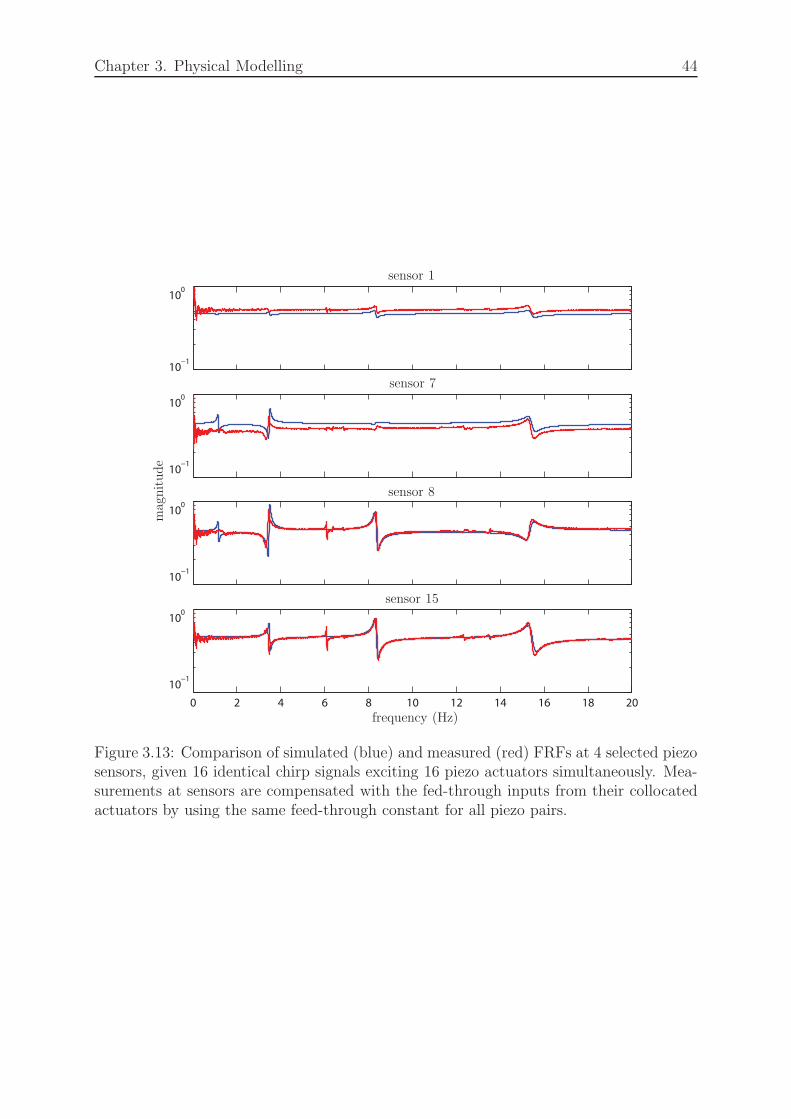
Chapter 3. Physical Modelling 44
10−1
100
10−1
100
10−1
100
0 2 4 6 8 10 12 14 16 18 20
10−1
100
sensor 1
sensor 7
sensor 8
sensor 15
frequency (Hz)
magnitude
Figure 3.13: Comparison of simulated (blue) and measured (red) FRFs at 4 selected piezosensors, given 16 identical chirp signals exciting 16 piezo actuators simultaneously. Mea-surements at sensors are compensated with the fed-through inputs from their collocatedactuators by using the same feed-through constant for all piezo pairs.

Chapter 3. Physical Modelling 45
−1
0
1
−1
0
1
−1
0
1
30 30.5 31 31.5 32 32.5 33 33.5 34
−1
0
1
sensor 1
sensor 7
sensor 8
sensor 15
time (s)
outputvoltage(V
)
Figure 3.14: Comparison of simulated (blue) and measured (red) output voltages at 4selected piezo sensors, given 16 noise signals exciting 16 piezo actuators simultaneously.The feed-through constants employed in the FE model are identical for all piezo pairs.

Chapter 4
Local LPV Identification of an FRFMatrix
4.1 Introdution
In Chapter 3, an FE-based modelling approach for the actuated structure accounting forthe coupled mechanical and piezoelectricity effect has been presented. However, from apractical point of view, this approach can involve tremendous experimental work, par-ticularly when a complex or a large-scale structure is encountered, where experimentsat a large number of actuating and sensing locations need to be performed to capturethe structural dynamics thoroughly. On the other hand, the lumped structure of the FEmodel is generally not suitable for a model-based controller design, due to its large systemorder.
Considering the combined FE method and experimental modal analysis as a white-boxidentification, this chapter addresses the above two issues of physical modelling, treat-ing the structure as a black box and identifying its FRF matrix by directly modellingits input/output behaviour, without exploring the physical insights into the structuraldynamics. It will be demonstrated that the FRF matrix of a structure even comprisedof physically identical subsystems exhibits spatially-varying characteristics. A local LPVidentification technique is extended from lumped systems to spatially-interconnected sys-tems. The FRFs at selected actuating and sensing locations are first identified as a setof LTI models, then parametrized as a spatial LPV model with the application of the ex-tended local approach. The FRFs at other locations can then be approximated throughinterpolation. In comparison to the physical modelling, the proposed approach facilitatesthe experimental work, at the price of a slightly deteriorated accuracy.
This chapter takes over results presented in [60], and is structured as follows: Section4.2 recaps the black-box identification techniques for both LTI and LPV lumped systems,whose signals are functions of time. The local approach for a temporal LPV modelidentification is extended later in this chapter to spatially-distributed systems. Section 4.3reviews the problems of current identification techniques and motivates the development ofa new approach. Taking a simple five-spring-mass-damper system as an example, Section
46
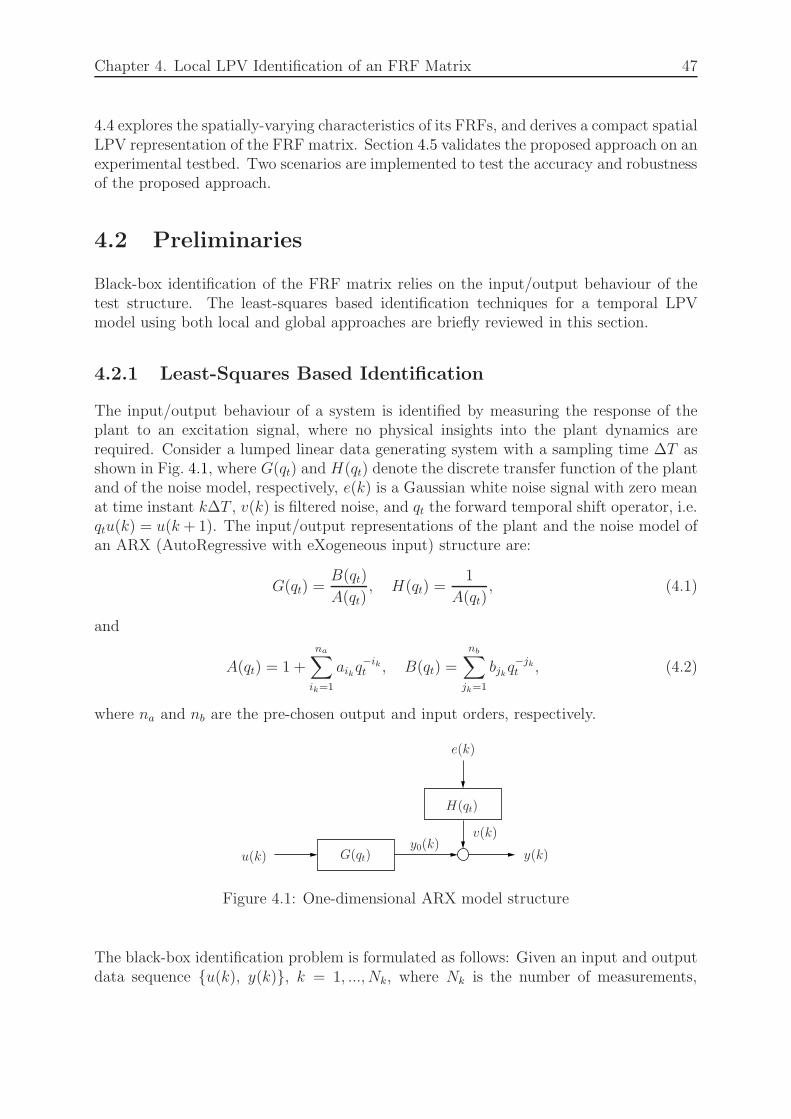
Chapter 4. Local LPV Identification of an FRF Matrix 47
4.4 explores the spatially-varying characteristics of its FRFs, and derives a compact spatialLPV representation of the FRF matrix. Section 4.5 validates the proposed approach on anexperimental testbed. Two scenarios are implemented to test the accuracy and robustnessof the proposed approach.
4.2 Preliminaries
Black-box identification of the FRF matrix relies on the input/output behaviour of thetest structure. The least-squares based identification techniques for a temporal LPVmodel using both local and global approaches are briefly reviewed in this section.
4.2.1 Least-Squares Based Identification
The input/output behaviour of a system is identified by measuring the response of theplant to an excitation signal, where no physical insights into the plant dynamics arerequired. Consider a lumped linear data generating system with a sampling time ∆T asshown in Fig. 4.1, where G(qt) and H(qt) denote the discrete transfer function of the plantand of the noise model, respectively, e(k) is a Gaussian white noise signal with zero meanat time instant k∆T , v(k) is filtered noise, and qt the forward temporal shift operator, i.e.qtu(k) = u(k + 1). The input/output representations of the plant and the noise model ofan ARX (AutoRegressive with eXogeneous input) structure are:
G(qt) =B(qt)
A(qt), H(qt) =
1
A(qt), (4.1)
and
A(qt) = 1 +
na∑
ik=1
aikq−ikt , B(qt) =
nb∑
jk=1
bjkq−jkt , (4.2)
where na and nb are the pre-chosen output and input orders, respectively.
u(k) G(qt)y0(k)
e(k)
H(qt)
v(k)
y(k)
Figure 4.1: One-dimensional ARX model structure
The black-box identification problem is formulated as follows: Given an input and outputdata sequence u(k), y(k), k = 1, ..., Nk, where Nk is the number of measurements,

Chapter 4. Local LPV Identification of an FRF Matrix 48
coefficients aik and bjk in G(qt) are to be estimated with the input and output orders na
and nb determined by trial and error, such that the cost function
J =
Nk∑
k=1
(y(k)− y(k))2 (4.3)
is minimized. The measured output is denoted as y(k), and the estimated output y(k) iscomputed by
y(k) = −na∑
ik=1
aiky(k − ik) +
nb∑
jk=1
bjku(k − jk). (4.4)
Restructure the difference equation (4.4) into regressor form
y(k) = φT (k)p, (4.5)
with a regressor vector
φ(k) =
[ [catik − y(k − ik)
]
ik=1:na[catjku(k − jk)
]
jk=1:nb
]
, (4.6)
and a parameter vector
p =
[ [catikaik
]
ik=1:na[catjkbjk
]
jk=1:nb
]
, (4.7)
where catik and catjk denote the concatenation of the coefficients in A(qt) and B(qt),respectively. For example, a system of an input order 2 and an output order 1, i.e. na = 2and nb = 1, gives rise to a parameter vector p = [a1, a2, b1]
T .
After constructing the data matrix Φ by augmenting the past inputs and outputs as
Φ = [φ(1), φ(2), · · · , φ(Nk)]T
and the output vectorY = [y(1), y(2), · · · , y(Nk)]
T ,
where Φ ∈ RNk×(na+nb), Y ∈ RNk , the least squares approach solves the estimation prob-lem by minimizing the cost function (4.3) with
p = (ΦTΦ)−1ΦTY, (4.8)
if Φ has full column rank.
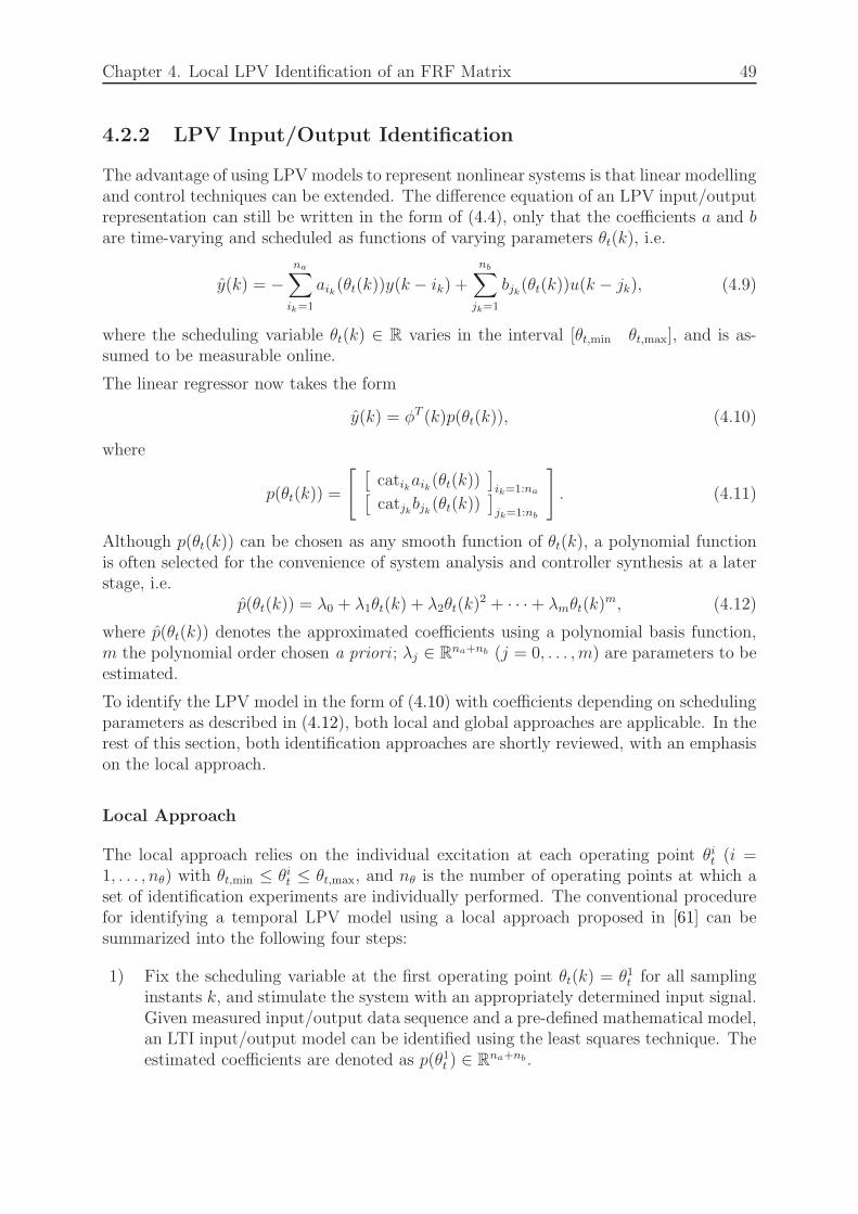
Chapter 4. Local LPV Identification of an FRF Matrix 49
4.2.2 LPV Input/Output Identification
The advantage of using LPVmodels to represent nonlinear systems is that linear modellingand control techniques can be extended. The difference equation of an LPV input/outputrepresentation can still be written in the form of (4.4), only that the coefficients a and bare time-varying and scheduled as functions of varying parameters θt(k), i.e.
y(k) = −na∑
ik=1
aik(θt(k))y(k − ik) +
nb∑
jk=1
bjk(θt(k))u(k − jk), (4.9)
where the scheduling variable θt(k) ∈ R varies in the interval [θt,min θt,max], and is as-sumed to be measurable online.
The linear regressor now takes the form
y(k) = φT (k)p(θt(k)), (4.10)
where
p(θt(k)) =
[ [catikaik(θt(k))
]
ik=1:na[catjkbjk(θt(k))
]
jk=1:nb
]
. (4.11)
Although p(θt(k)) can be chosen as any smooth function of θt(k), a polynomial functionis often selected for the convenience of system analysis and controller synthesis at a laterstage, i.e.
p(θt(k)) = λ0 + λ1θt(k) + λ2θt(k)2 + · · ·+ λmθt(k)
m, (4.12)
where p(θt(k)) denotes the approximated coefficients using a polynomial basis function,m the polynomial order chosen a priori ; λj ∈ Rna+nb (j = 0, . . . , m) are parameters to beestimated.
To identify the LPV model in the form of (4.10) with coefficients depending on schedulingparameters as described in (4.12), both local and global approaches are applicable. In therest of this section, both identification approaches are shortly reviewed, with an emphasison the local approach.
Local Approach
The local approach relies on the individual excitation at each operating point θit (i =1, . . . , nθ) with θt,min ≤ θit ≤ θt,max, and nθ is the number of operating points at which aset of identification experiments are individually performed. The conventional procedurefor identifying a temporal LPV model using a local approach proposed in [61] can besummarized into the following four steps:
1) Fix the scheduling variable at the first operating point θt(k) = θ1t for all samplinginstants k, and stimulate the system with an appropriately determined input signal.Given measured input/output data sequence and a pre-defined mathematical model,an LTI input/output model can be identified using the least squares technique. Theestimated coefficients are denoted as p(θ1t ) ∈ R
na+nb.
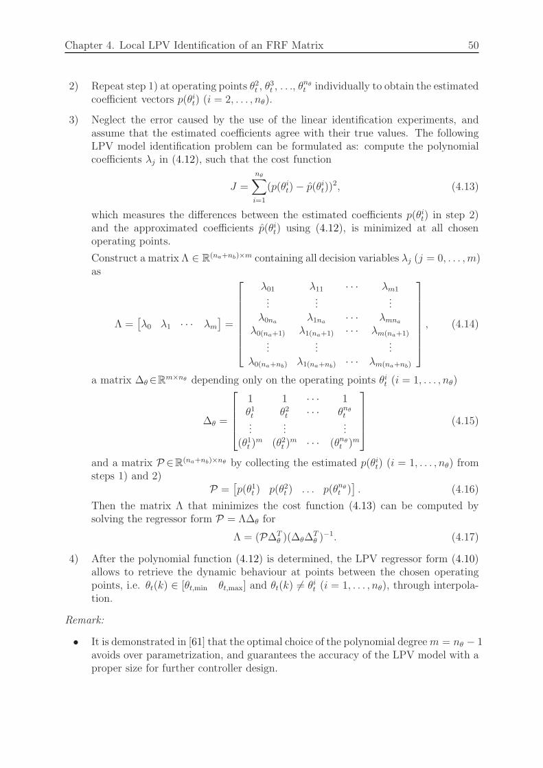
Chapter 4. Local LPV Identification of an FRF Matrix 50
2) Repeat step 1) at operating points θ2t , θ3t , . . ., θ
nθ
t individually to obtain the estimatedcoefficient vectors p(θit) (i = 2, . . . , nθ).
3) Neglect the error caused by the use of the linear identification experiments, andassume that the estimated coefficients agree with their true values. The followingLPV model identification problem can be formulated as: compute the polynomialcoefficients λj in (4.12), such that the cost function
J =
nθ∑
i=1
(p(θit)− p(θit))2, (4.13)
which measures the differences between the estimated coefficients p(θit) in step 2)and the approximated coefficients p(θit) using (4.12), is minimized at all chosenoperating points.
Construct a matrix Λ ∈ R(na+nb)×m containing all decision variables λj (j = 0, . . . , m)as
Λ =[λ0 λ1 · · · λm
]=
λ01 λ11 · · · λm1...
......
λ0naλ1na
· · · λmna
λ0(na+1) λ1(na+1) · · · λm(na+1)...
......
λ0(na+nb) λ1(na+nb) · · · λm(na+nb)
, (4.14)
a matrix ∆θ∈Rm×nθ depending only on the operating points θit (i = 1, . . . , nθ)
∆θ =
1 1 · · · 1θ1t θ2t · · · θnθ
t...
......
(θ1t )m (θ2t )
m · · · (θnθ
t )m
(4.15)
and a matrix P ∈R(na+nb)×nθ by collecting the estimated p(θit) (i = 1, . . . , nθ) fromsteps 1) and 2)
P =[p(θ1t ) p(θ2t ) . . . p(θnθ
t )]. (4.16)
Then the matrix Λ that minimizes the cost function (4.13) can be computed bysolving the regressor form P = Λ∆θ for
Λ = (P∆Tθ )(∆θ∆
Tθ )
−1. (4.17)
4) After the polynomial function (4.12) is determined, the LPV regressor form (4.10)allows to retrieve the dynamic behaviour at points between the chosen operatingpoints, i.e. θt(k) ∈ [θt,min θt,max] and θt(k) 6= θit (i = 1, . . . , nθ), through interpola-tion.
Remark:
• It is demonstrated in [61] that the optimal choice of the polynomial degreem = nθ − 1avoids over parametrization, and guarantees the accuracy of the LPV model with aproper size for further controller design.

Chapter 4. Local LPV Identification of an FRF Matrix 51
Global Approach
Instead of identifying the system dynamics at a set of fixed scheduling parameters usingthe local approach, the global approach allows to stimulate the system via one singleexperiment with a large number of operating points excited to determine the functionaldependence ([62], [63]). In case of a polynomial dependence, conditions on persistency ofexcitation in terms of inputs and trajectories of scheduling parameters are discussed in [28],where the estimation problem is solved through the recursive least squares algorithms. InChapter 5, the global approach will be applied for the identification of a two-dimensionalLPV input/output model.
4.3 Problem Statement
It has been illustrated in Chapter 3 that the FE modelling discretizes a continuous struc-ture into an array of interconnected subsystems, with the dynamics of each subsystemcaptured by a spring-mass-damper system. Consider a system as shown in Fig. 4.2. Itconsists of 5 spring-mass-damper systems, each governed by the equation of motion
f = my + cy + ky, (4.18)
where m, k, and c are the elemental (in this case, scalar) mass, stiffness and damping,respectively, f is the exogenous force, and y the mass deflection. The viscous damping crepresents the energy dissipation mechanisms, and it is typically not known exactly. Forsimplicity, a proportional damping
c = αm+ βk (4.19)
is assumed, where α and β are tunable coefficients. Let the global mass, stiffness anddamping matrices be denoted as M, K, and C, respectively. The global dynamics of theinterconnected spring-mass-damper system are governed by
F = MY + CY +KY, (4.20)
where F and Y are the input force vector and the output deflection vector, respectively,i.e. F = [f1, f2, f3, f4, f5]
T and Y = [y1, y2, y3, y4, y5]T . A free-free boundary condition is
fulfilled, as no restriction is applied to the boundary subsystems. It is obvious that eachsubsystem is capable of actuating and sensing.
f1 y1 f2y2 f3
y3 f4y4 f5
y5
k kkkmmmmm
c ccc
Figure 4.2: Interconnected spring-mass-damper system consisting of 5 subsystems

Chapter 4. Local LPV Identification of an FRF Matrix 52
Assume that the mass, the stiffness, and the damping are identical for all subsystems.Let the values be m = 1 kg, k = 10 N/m, α = 10−3 and β = 10−4. The global mass andstiffness matrices are
M =
1 0 0 0 00 1 0 0 00 0 1 0 00 0 0 1 00 0 0 0 1
K =
10 −10 0 0 0−10 20 −10 0 00 −10 20 −10 00 0 −10 20 −100 0 0 −10 10
, (4.21)
respectively. The appication of the Laplace transform to (4.20) results in
G(s) = [Ms2 + Cs +K]−1, (4.22)
where G(s) is the continuous MIMO transfer function matrix from F to Y , or the so-called FRF matrix in the field of structural engineering. Its dimension is determined bythe number of inputs and outputs, or in this context the number of spatially discretizedsubsystems.
The symmetric mass, damping and stiffness matrices imply a symmetric transfer functionmatrix G(s), and further the structural reciprocity ([56], [64]) of a linear system: thetransfer function from a single input at coordinate i to the output at j is the same as thetransfer function from an input at j to output at i. After the temporal discretization, thecontinuous and symmetric G(s) is converted into
G(qt) =
G11(qt) G12(qt) G13(qt) G14(qt) G15(qt)G22(qt) G23(qt) G24(qt) G25(qt)
G33(qt) G34(qt) G35(qt)sym G44(qt) G45(qt)
G55(qt)
, (4.23)
where the operator Gij(qt) denotes the transfer function, or FRF, from the excitation atj to response at i (i, j = 1, . . . , 5), ’sym’ the symmetric components in a matrix. Whenthe coordinates of i and j coincide, i.e. i = j, the FRF is referred to as a point FRF,otherwise a transfer FRF. In the rest of this chapter, G and Gij are used to denote theFRF matrix G(qt) and the operator Gij(qt), respectively, for notational simplicity.
Both (4.20) and (4.23) describe the global dynamics of the system in Fig. 4.2. Now supposethat the elemental m, k, and c are not known accurately, and need to be estimated. Themodelling of (4.20) relies on the knowledge of system physics in terms of its mass, stiffnessand damping matrices, and falls into the FE modelling that has been extensively discussedin Chapter 3. The obtained FE model is generally not suitable for a model-based controllersynthesis, due to its generally high system order.
The conventional black-box identification of (4.23) relies on the input/output behaviourof the system. Each operator Gij is treated as an LTI system, and identified individually:given the single-input and single-output (SISO) data set (uj, yi), Gij is identified byapplying the least-squares method discussed in Section 4.2.1, where na and nb determiningthe model structure are chosen a priori. Experiments and identification procedures are

Chapter 4. Local LPV Identification of an FRF Matrix 53
then repeatedly performed, until all upper triangular operators in (4.23) are estimated.Despite of its simplicity, the conventional black-box identification of (4.23) fails to be aneffective approach due to the following two reasons:
1) The identification of any operator Gij in the FRF matrix requires the single exci-tation at subsystem j and measured response of subsystem i. When a large-scalestructure that consists of a large number of inputs and outputs is encountered,the experimental data acquisition process may become tremendous and tedious, interms of repeating the experiments. The same is true for the estimation process.
2) For control engineers, system identification is performed to obtain an accurate math-ematical model, whose structure is suitable for an effective controller design. It isdesired in control of distributed parameter systems that the controller inherits thedistributed structure of the plant, i.e.
K =
K11 K12 K13 K14 K15
K22 K23 K24 K25
K33 K34 K35
sym K44 K45
K55
. (4.24)
Given the fact that each operator Gij in (4.23) is determined individually, so isthe controller operator Kij in (4.24). The involved work makes the plant structureunfavourable from a practical point of view.
Driven by the above two drawbacks of the conventional black-box identification technique,a novel identification approach is needed. The identified model should preserve the accu-racy achieved by the conventional technique to a certain extent. In addition, the resultingplant structure should lead to an efficient system identification and controller synthesisprocess, which involves a reasonable amount of effort, even when dealing with a complexor large-scale system.
4.4 LPV Identification of an FRF Matrix
To address the two issues related to the individual identification of the FRFs in (4.23),a spatial LPV model is proposed to capture the spatially-varying characteristics of theFRF matrix. To justify this approach, the system in Fig. 4.2 is taken as an example todemonstrate the varying properties of the FRFs, and how this variation leads to a spatialLPV representation.
4.4.1 Spatially-Varying Characteristics of FRFs
Due to the interconnection between subsystems through springs and dampers, the dynam-ics of the 5 subsystems in Fig. 4.2 are clearly not decoupled, but interacting with nearest
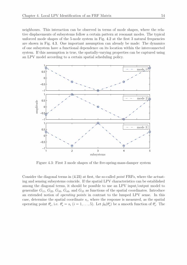
Chapter 4. Local LPV Identification of an FRF Matrix 54
neighbours. This interaction can be observed in terms of mode shapes, where the rela-tive displacements of subsystems follow a certain pattern at resonant modes. The typicalunforced mode shapes of the 5-node system in Fig. 4.2 at the first 3 natural frequenciesare shown in Fig. 4.3. One important assumption can already be made: The dynamicsof one subsystem have a functional dependence on its location within the interconnectedsystem. If this assumption is true, the spatially-varying properties can be captured usingan LPV model according to a certain spatial scheduling policy.
−1
−0.5
0
0.5
1
−1
−0.5
0
0.5
1
1 2 3 4 5−1
−0.5
0
0.5
1
mode 1
mode 2
mode 3
amplitude
subsystems
Figure 4.3: First 3 mode shapes of the five-spring-mass-damper system
Consider the diagonal terms in (4.23) at first, the so-called point FRFs, where the actuat-ing and sensing subsystems coincide. If the spatial LPV characteristics can be establishedamong the diagonal terms, it should be possible to use an LPV input/output model togeneralize G11, G22, G33, G44, and G55 as functions of the spatial coordinates. Introducean extended notion of operating points in contrast to the lumped LPV sense. In thiscase, determine the spatial coordinate si, where the response is measured, as the spatialoperating point θis, i.e. θ
is = si (i = 1, . . . , 5). Let p0(θ
is) be a smooth function of θis. The

Chapter 4. Local LPV Identification of an FRF Matrix 55
diagonal terms can be represented in LPV form as
G =
G(p0(θ1s)) G12 G13 G14 G15
G(p0(θ2s)) G23 G24 G25
G(p0(θ3s)) G34 G35
sym G(p0(θ4s)) G45
G(p0(θ5s))
. (4.25)
The spatial LPVmodelG(p0(θis)) differs from (4.9) in terms of the scheduling parameters—
time-varying in a lumped system, time/space-varying in a spatially-distributed system.The subscript 0 indicates the diagonal terms.
The true values of p0(θis) can be first estimated by applying the conventional black-box
identification technique to individually identify the LTI operators Gii (i = 1, . . . , 5) asdescribed in steps 1) and 2) in Section 4.2.2, except that the fixed operating points arespatial variables here. Approximate p0(θ
is) with a polynomial function p0(θ
is) of θis. An
LPV representation of the 5 diagonal terms in (4.25) can then be easily derived followingstep 3) in Section 4.2.2. It is evident that if a solution to (4.17) exists, the approximatedpolynomial coefficients p0(θ
is) agree with the true values p0(θ
is) (i = 1, . . . , 5).
To explore the advantages of using an LPV model to generalize the diagonal terms (4.25),now assume that identification experiments can not be implemented at all operating pointsdue to certain constraints. For example, the LTI operators G11, G33, G44 and G55 can beexperimentally identified, whereas it is not possible to perform actuating and/or sensingat subsystem 2, so that G22 needs to be determined without performing an experiment.This problem can be solved by first constructing an LPV model G(p0(θ
is)) based on the
information at operating points θ1s , θ3s , θ
4s and θ5s , then interpolating θ2s in G(p0(θ
is)) to
obtain G22. Fig. 4.4 shows a comparison between two FRFs of G22: one is its true value;the other one is simulated from G(p0(θ
2s)). Although the interpolated operator is lightly
damped at the 2nd mode, the resonant peaks at other modes are well preserved. Themain dynamics are captured in spite of a degraded accuracy. The modelling error maybe attributed to a functional dependence of p0(θ
is) on θis of a higher complexity than the
simple polynomial function assumed here.
The 1st off-diagonal terms are the transfer FRFs from the single excitation at subsystemj = i+1 to measured response at subsystem i (i = 1, . . . , 4). Applying similar proceduresas above to identify operators Gi(i+1) (i = 1, . . . , 4) results in another set of LPV modelsG(p1(θ
is)) (i = 1, . . . , 4)
G =
G11 G(p1(θ1s)) G13 G14 G15
G22 G(p1(θ2s)) G24 G25
G33 G(p1(θ3s)) G35
sym G44 G(p1(θ4s))
G55
, (4.26)
where the same scheduling policy as for the diagonal terms is employed, i.e., the spatialoperating points are the spatial coordinates where the responses are measured.
The identified spatial LPV model also allows the interpolation of operating points wherethe identification experiments are not performed. Suppose that the response at subsystem 1
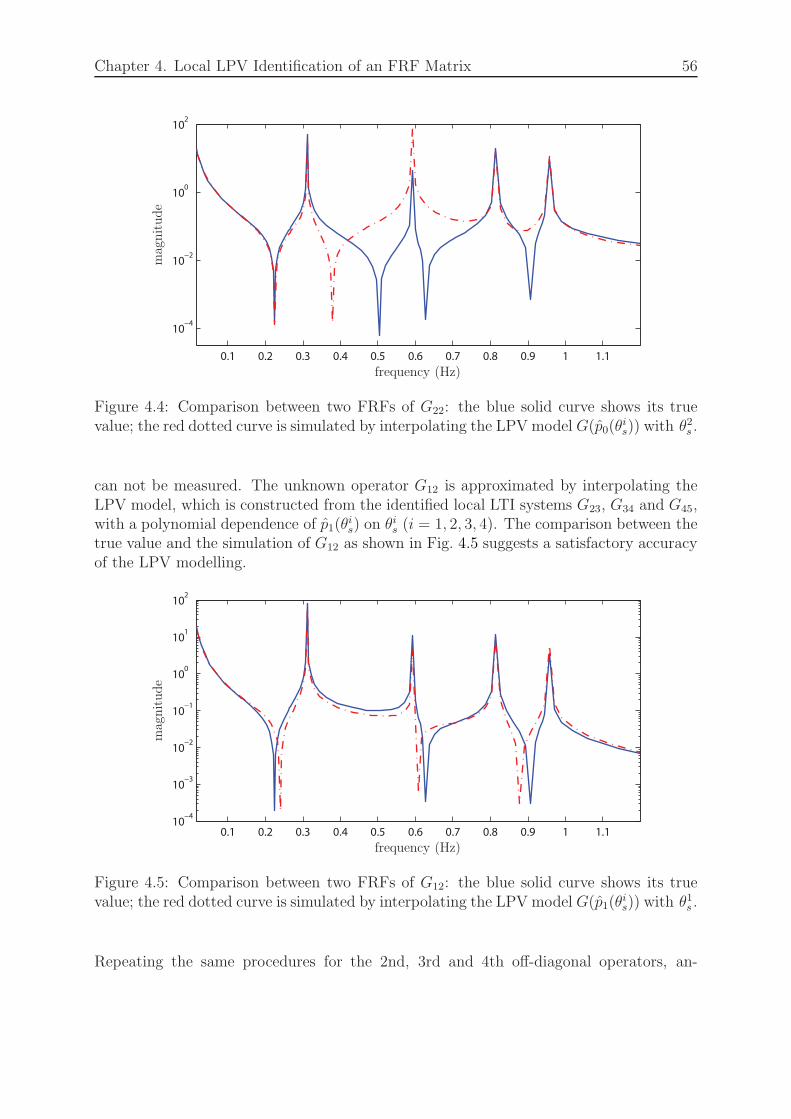
Chapter 4. Local LPV Identification of an FRF Matrix 56
0.1 0.2 0.3 0.4 0.5 0.6 0.7 0.8 0.9 1 1.1
10−4
10−2
100
102
frequency (Hz)
magnitude
Figure 4.4: Comparison between two FRFs of G22: the blue solid curve shows its truevalue; the red dotted curve is simulated by interpolating the LPV model G(p0(θ
is)) with θ2s .
can not be measured. The unknown operator G12 is approximated by interpolating theLPV model, which is constructed from the identified local LTI systems G23, G34 and G45,with a polynomial dependence of p1(θ
is) on θis (i = 1, 2, 3, 4). The comparison between the
true value and the simulation of G12 as shown in Fig. 4.5 suggests a satisfactory accuracyof the LPV modelling.
0.1 0.2 0.3 0.4 0.5 0.6 0.7 0.8 0.9 1 1.110
−4
10−3
10−2
10−1
100
101
102
frequency (Hz)
magnitude
Figure 4.5: Comparison between two FRFs of G12: the blue solid curve shows its truevalue; the red dotted curve is simulated by interpolating the LPV model G(p1(θ
is)) with θ1s .
Repeating the same procedures for the 2nd, 3rd and 4th off-diagonal operators, an-
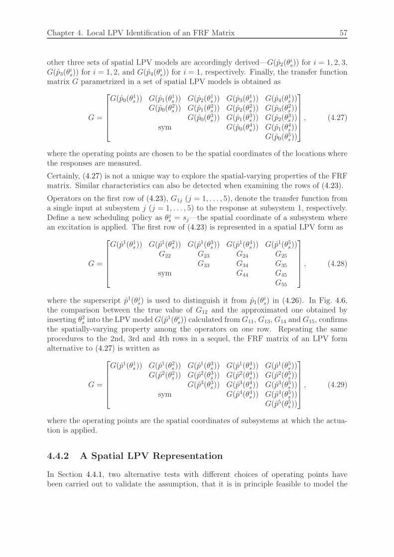
Chapter 4. Local LPV Identification of an FRF Matrix 57
other three sets of spatial LPV models are accordingly derived—G(p2(θis)) for i = 1, 2, 3,
G(p3(θis)) for i = 1, 2, and G(p4(θ
is)) for i = 1, respectively. Finally, the transfer function
matrix G parametrized in a set of spatial LPV models is obtained as
G =
G(p0(θ1s)) G(p1(θ
1s)) G(p2(θ
1s)) G(p3(θ
1s)) G(p4(θ
1s))
G(p0(θ2s)) G(p1(θ
2s)) G(p2(θ
2s)) G(p3(θ
2s))
G(p0(θ3s)) G(p1(θ
3s)) G(p2(θ
3s))
sym G(p0(θ4s)) G(p1(θ
4s))
G(p0(θ5s))
, (4.27)
where the operating points are chosen to be the spatial coordinates of the locations wherethe responses are measured.
Certainly, (4.27) is not a unique way to explore the spatial-varying properties of the FRFmatrix. Similar characteristics can also be detected when examining the rows of (4.23).
Operators on the first row of (4.23), G1j (j = 1, . . . , 5), denote the transfer function froma single input at subsystem j (j = 1, . . . , 5) to the response at subsystem 1, respectively.Define a new scheduling policy as θjs = sj—the spatial coordinate of a subsystem wherean excitation is applied. The first row of (4.23) is represented in a spatial LPV form as
G =
G(p1(θ1s)) G(p1(θ2s)) G(p1(θ3s)) G(p1(θ4s)) G(p1(θ5s))G22 G23 G24 G25
G33 G34 G35
sym G44 G45
G55
, (4.28)
where the superscript p1(θjs) is used to distinguish it from p1(θis) in (4.26). In Fig. 4.6,
the comparison between the true value of G12 and the approximated one obtained byinserting θ2s into the LPV model G(p1(θis)) calculated fromG11, G13, G14 and G15, confirmsthe spatially-varying property among the operators on one row. Repeating the sameprocedures to the 2nd, 3rd and 4th rows in a sequel, the FRF matrix of an LPV formalternative to (4.27) is written as
G =
G(p1(θ1s)) G(p1(θ2s)) G(p1(θ3s)) G(p1(θ4s)) G(p1(θ5s))G(p2(θ2s)) G(p2(θ3s)) G(p2(θ4s)) G(p2(θ5s))
G(p3(θ3s)) G(p3(θ4s)) G(p3(θ5s))sym G(p4(θ4s)) G(p4(θ5s))
G(p5(θ5s))
, (4.29)
where the operating points are the spatial coordinates of subsystems at which the actua-tion is applied.
4.4.2 A Spatial LPV Representation
In Section 4.4.1, two alternative tests with different choices of operating points havebeen carried out to validate the assumption, that it is in principle feasible to model the
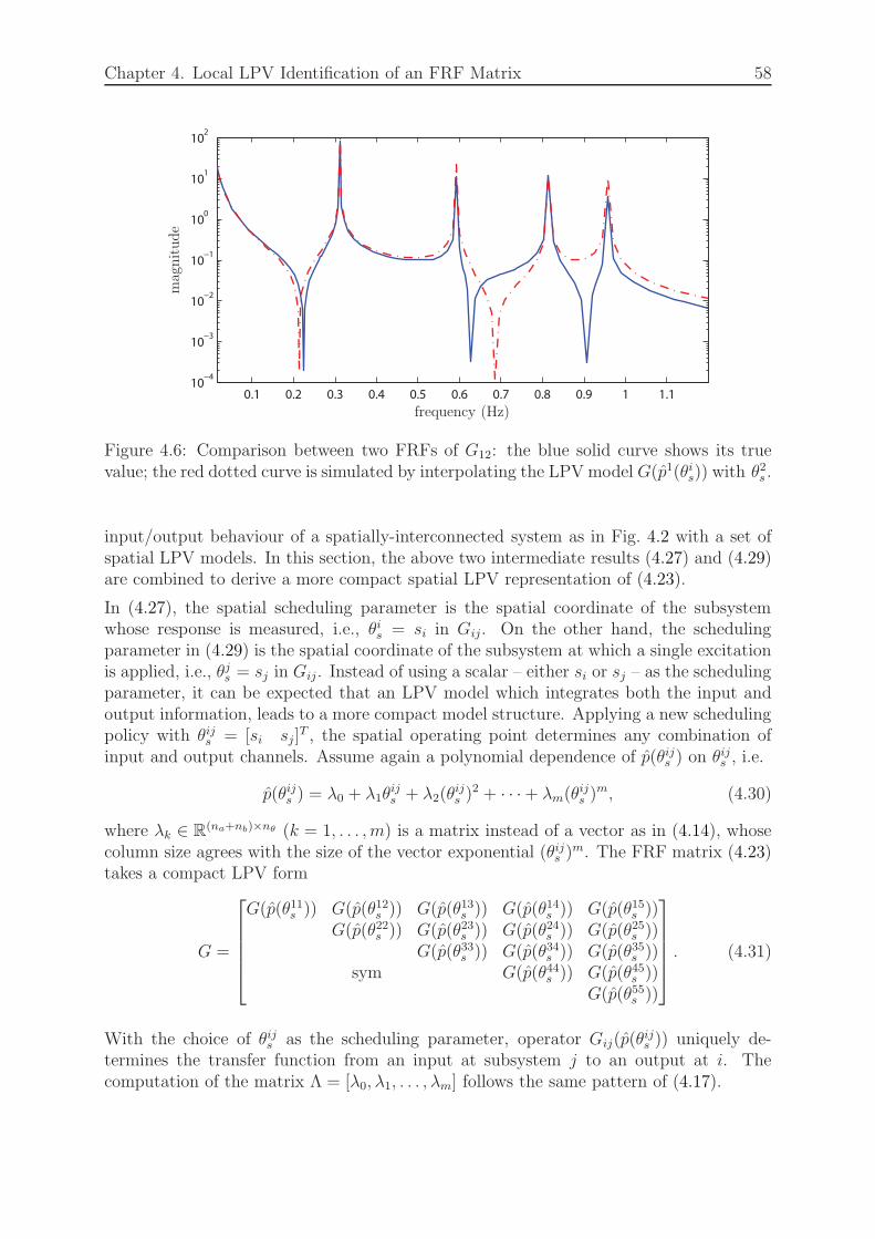
Chapter 4. Local LPV Identification of an FRF Matrix 58
0.1 0.2 0.3 0.4 0.5 0.6 0.7 0.8 0.9 1 1.110
−4
10−3
10−2
10−1
100
101
102
frequency (Hz)
magnitude
Figure 4.6: Comparison between two FRFs of G12: the blue solid curve shows its truevalue; the red dotted curve is simulated by interpolating the LPV model G(p1(θis)) with θ2s .
input/output behaviour of a spatially-interconnected system as in Fig. 4.2 with a set ofspatial LPV models. In this section, the above two intermediate results (4.27) and (4.29)are combined to derive a more compact spatial LPV representation of (4.23).
In (4.27), the spatial scheduling parameter is the spatial coordinate of the subsystemwhose response is measured, i.e., θis = si in Gij. On the other hand, the schedulingparameter in (4.29) is the spatial coordinate of the subsystem at which a single excitationis applied, i.e., θjs = sj in Gij. Instead of using a scalar – either si or sj – as the schedulingparameter, it can be expected that an LPV model which integrates both the input andoutput information, leads to a more compact model structure. Applying a new schedulingpolicy with θijs = [si sj]
T , the spatial operating point determines any combination ofinput and output channels. Assume again a polynomial dependence of p(θijs ) on θijs , i.e.
p(θijs ) = λ0 + λ1θijs + λ2(θ
ijs )
2 + · · ·+ λm(θijs )
m, (4.30)
where λk ∈ R(na+nb)×nθ (k = 1, . . . , m) is a matrix instead of a vector as in (4.14), whosecolumn size agrees with the size of the vector exponential (θijs )
m. The FRF matrix (4.23)takes a compact LPV form
G =
G(p(θ11s )) G(p(θ12s )) G(p(θ13s )) G(p(θ14s )) G(p(θ15s ))G(p(θ22s )) G(p(θ23s )) G(p(θ24s )) G(p(θ25s ))
G(p(θ33s )) G(p(θ34s )) G(p(θ35s ))sym G(p(θ44s )) G(p(θ45s ))
G(p(θ55s ))
. (4.31)
With the choice of θijs as the scheduling parameter, operator Gij(p(θijs )) uniquely de-
termines the transfer function from an input at subsystem j to an output at i. Thecomputation of the matrix Λ = [λ0, λ1, . . . , λm] follows the same pattern of (4.17).
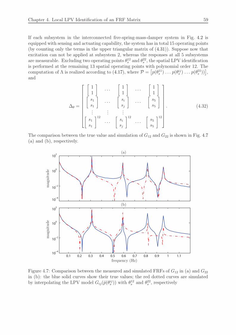
Chapter 4. Local LPV Identification of an FRF Matrix 59
If each subsystem in the interconnected five-spring-mass-damper system in Fig. 4.2 isequipped with sensing and actuating capability, the system has in total 15 operating points(by counting only the terms in the upper triangular matrix of (4.31)). Suppose now thatexcitation can not be applied at subsystem 2, whereas the responses at all 5 subsystemsare measurable. Excluding two operating points θ12s and θ22s , the spatial LPV identificationis performed at the remaining 13 spatial operating points with polynomial order 12. Thecomputation of Λ is realized according to (4.17), where P =
[p(θ11s ) . . . p(θijs ) . . . p(θ
55s ))],
and
∆θ =
[11
]
· · ·[11
]
· · ·[11
]
[s1s1
]
· · ·[sisj
]
· · ·[s5s5
]
......
...[s1s1
]12
· · ·[sisj
]12
· · ·[s5s5
]12
. (4.32)
The comparison between the true value and simulation of G12 and G22 is shown in Fig. 4.7(a) and (b), respectively.
10−4
10−2
100
102
0.1 0.2 0.3 0.4 0.5 0.6 0.7 0.8 0.9 1 1.110
−4
10−2
100
102
frequency (Hz)
magnitude
magnitude
(a)
(b)
Figure 4.7: Comparison between the measured and simulated FRFs of G12 in (a) and G22
in (b): the blue solid curves show their true values; the red dotted curves are simulatedby interpolating the LPV model Gij(p(θ
ijs )) with θ12s and θ22s , respectively
Chapter 4. Local LPV Identification of an FRF Matrix 60
Remarks:
• The benefits of using a spatial LPV model to parametrize the FRF matrix becomemore obvious when a large-scale system needs to be identified. Instead of performingthe identification experiments at each spatial operating point, the spatial LPV struc-ture allows to select some crucial points to perform the identification experiments,whereas the FRFs at other locations can be estimated through LPV interpolation.
• The spatial LPV plant model (4.31) leads to an efficient controller design process,where the controller inherits the spatial LPV structure as
K =
K(p(θ11s )) K(p(θ12s )) K(p(θ13s )) K(p(θ14s )) K(p(θ15s ))K(p(θ22s )) K(p(θ23s )) K(p(θ24s )) K(p(θ25s ))
K(p(θ33s )) K(p(θ34s )) K(p(θ35s ))sym K(p(θ44s )) K(p(θ45s ))
K(p(θ55s ))
. (4.33)
• Since a vector exponential involves cross product terms, e.g. (θijs )2 = [s2i , s
2j , sisj ]
T ,it may significantly increase the size of (4.32) and thus the computational burdenof the optimization problem (4.17). Nevertheless, experience shows that even withan elementwise vector exponential, the identified LPV model demonstrates a satis-factory accuracy.
• It has been explained in [6] that the interaction between subsystems shows an expo-nential decay in space: the larger the distance between two subsystems, the smallerthe impact. The implementation of spatial truncation leads to a ’localized’ struc-ture whose dynamics are close to the original system, but only influenced by theneighbouring subsystems. Therefore, when dealing with a system that consists of alarge number of subsystems, instead of a full transfer function matrix G, a bandedmatrix
G′ =
∗ · · · ∗∗ · · · ∗ 0
∗ · · · ∗0 ∗ · · · ∗
∗ · · · ∗
(4.34)
appears to be a more attractive structure from a practical point of view, afterspatially truncating the operators Gij when |sj − si| > γ, where γ is the maximumallowable distance from input to output. The truncated FRF matrix coincides withthe structure of a distributed system, in the sense that the response of one subsystemis determined by itself and its nearest neighbours.
• Increasing the number of the operating points at which the identification experi-ments are performed leads to a higher accuracy of the identified model at the costof increased computational complexity. A compromise between the model accuracyand complexity needs to be achieved according to the requirements. On the otherhand, given a fixed number of operating points, the optimization of their locationsto achieve a maximum accuracy is discussed in [61] .
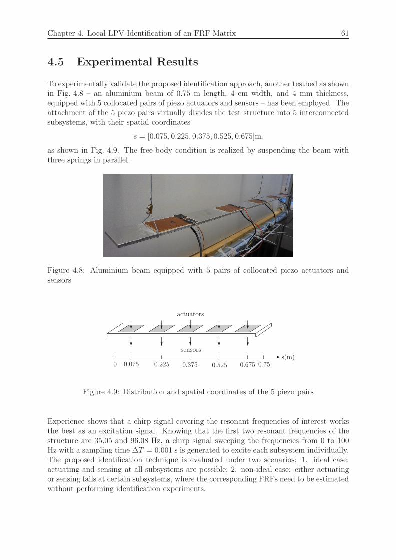
Chapter 4. Local LPV Identification of an FRF Matrix 61
4.5 Experimental Results
To experimentally validate the proposed identification approach, another testbed as shownin Fig. 4.8 – an aluminium beam of 0.75 m length, 4 cm width, and 4 mm thickness,equipped with 5 collocated pairs of piezo actuators and sensors – has been employed. Theattachment of the 5 piezo pairs virtually divides the test structure into 5 interconnectedsubsystems, with their spatial coordinates
s = [0.075, 0.225, 0.375, 0.525, 0.675]m,
as shown in Fig. 4.9. The free-body condition is realized by suspending the beam withthree springs in parallel.
Figure 4.8: Aluminium beam equipped with 5 pairs of collocated piezo actuators andsensors
actuators
sensors
0 0.075 0.225 0.375 0.525 0.675 0.75s(m)
Figure 4.9: Distribution and spatial coordinates of the 5 piezo pairs
Experience shows that a chirp signal covering the resonant frequencies of interest worksthe best as an excitation signal. Knowing that the first two resonant frequencies of thestructure are 35.05 and 96.08 Hz, a chirp signal sweeping the frequencies from 0 to 100Hz with a sampling time ∆T = 0.001 s is generated to excite each subsystem individually.The proposed identification technique is evaluated under two scenarios: 1. ideal case:actuating and sensing at all subsystems are possible; 2. non-ideal case: either actuatingor sensing fails at certain subsystems, where the corresponding FRFs need to be estimatedwithout performing identification experiments.
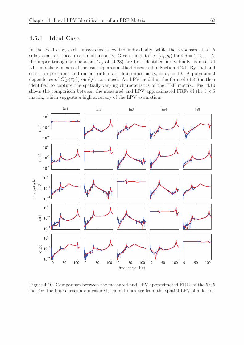
Chapter 4. Local LPV Identification of an FRF Matrix 62
4.5.1 Ideal Case
In the ideal case, each subsystems is excited individually, while the responses at all 5subsystems are measured simultaneously. Given the data set (uj, yi) for i, j = 1, 2, . . . , 5,the upper triangular operators Gij of (4.23) are first identified individually as a set ofLTI models by means of the least-squares method discussed in Section 4.2.1. By trial anderror, proper input and output orders are determined as na = nb = 10. A polynomialdependence of G(p(θijs )) on θijs is assumed. An LPV model in the form of (4.31) is thenidentified to capture the spatially-varying characteristics of the FRF matrix. Fig. 4.10shows the comparison between the measured and LPV approximated FRFs of the 5 × 5matrix, which suggests a high accuracy of the LPV estimation.
10−4
10−2
100
10−4
10−2
100
10−4
10−2
100
10−4
10−2
100
0 50 100
10−4
10−2
100
0 50 100 0 50 100 0 50 100 0 50 100
in1 in2 in3 in4 in5
out1
out2
out3
out4
out5
magnitude
frequency (Hz)
Figure 4.10: Comparison between the measured and LPV approximated FRFs of the 5×5matrix: the blue curves are measured; the red ones are from the spatial LPV simulation.

Chapter 4. Local LPV Identification of an FRF Matrix 63
4.5.2 Non-ideal Case
The non-ideal scenario is meant to test the reliability of the local LPV identificationtechnique, when performing identification experiments at certain operating points is notpossible.
Assume that the 3rd actuator is defect, i.e. the operators G13, G23 and G33 in (4.23) cannot be identified experimentally, but can be approximated, after a spatial LPV modelG(p(θijs )) is constructed based on the information at available operating points. Fig. 4.11shows the comparison between the measured and simulated FRFs of G13 in (a), G23 in(b) and G33 in (c). Though some discrepancies exist, the structural dynamics at the firsttwo modes are relatively well preserved.
10−5
100
10−5
100
0 10 20 30 40 50 60 70 80 90 100 110
10−1
100
frequency (Hz)
magnitude
(a)
(b)
(c)
Figure 4.11: Comparison of the measured and simulated FRFs ofG13 in (a), G23 in (b) andG33 in (c): the blue curves are measured; the red curves are from interpolating the LPVmodel G(p(θijs )) with θ13s , θ23s , and θ33s , respectively, assumed that the 3rd actuator fails.
4.6 Summary
This chapter has proposed a novel approach to identify the FRF matrix directly fromthe input/output behaviour of a test structure, to address two issues that arise from
Chapter 4. Local LPV Identification of an FRF Matrix 64
implementing the conventional black-box identification: 1. the individual identificationof the FRFs in an FRF matrix requires performing identification experiments at a largenumber of actuating and sensing locations, when dealing with a large-scale or complexstructure; 2. the structure of the identified FRF matrix is generally not suitable forcontroller design. It has been demonstrated step by step that the FRFs in an FRF matrixexhibit spatially-varying characteristics. A local LPV identification approach has beenextended from lumped systems to spatially-distributed systems. The FRF matrix canthen be parametrized as a spatial LPV model, which allows to approximate the FRFs atnon-actuated/non-sensed locations through LPV interpolation. The proposed approachfacilitates the experimental work by allowing to perform experiments at a relatively smallnumber of selected actuating and sensing locations. Meanwhile, the LPV representationof the FRF matrix enables an efficient LPV controller design, if a controller that inheritsthe plant structure is required. The performance of the proposed approach has beenexperimentally demonstrated on an actuated beam. When actuating and/or sensing atcertain locations is not possible, FRFs approximated through the LPV interpolation stillpreserve the main dynamics of the test structure.

Chapter 5
Distributed Identification
5.1 Introduction
Although Chapter 3 and Chapter 4 have dealt with the physical modelling and lumpedidentification of given test structures, respectively, the obtained models do not allow towork in the framework developed in Chapter 2. Thus a mathematical model that capturesthe distributed nature of a structure is needed, such that system analysis and controllersynthesis conditions first developed in [8] can be applied.
It is well-known that the mechanical behaviour of structures is typically governed byPDEs. The FE method presented in Chapter 3 is one technique to solve for the ap-proximated solutions to PDEs. In this chapter, an alternative numerical technique –the finite difference (FD) method – is discussed. The application of the FD methodleads to a two-dimensional input/output model structure, which spatially discretizes thedistributed-parameter system into interconnected subsystems, and defines the system dy-namics on an individual subsystem of a small order. The resulting input/output modelcan then be converted into the state space form that lends itself to efficient, LMI-basedsynthesis of distributed control; it is thus used as the mathematical model for a distributedidentification.
This chapter considers the distributed identification of both parameter-invariant andparameter-varying models. The input/output identification techniques developed in [27]for LTSI models and in [29] for spatial LPV models are implemented experimentally.A new identification approach that exploits the physical modelling results obtained inChapter 3 is proposed here to improve the identification accuracy, with the desired math-ematical model still preserved.
This chapter includes results reported in [65] and [66]. It is organized as follows: Section5.2 derives the mathematical model for distributed identification by solving PDEs usingthe FD method. Section 5.3 briefly reviews the input/output identification techniques forboth LTSI and spatial LPV models developed in [27] and [29], respectively, and tests themon the test structure. Section 5.4 develops an alternative identification procedure, which
65

Chapter 5. Distributed Identification 66
accounts for the physical properties of the test structure and experimentally demonstratesa better performance compared to black-box identification.
5.2 Mathematical Model for Identification
This section discusses the implementation of the FD method to solve for approximatesolutions to the governing PDE of a beam structure. The resulting two-dimensionalinput/output model structure captures the dynamics of spatially-discrete subsystems in-teracting with nearest neighbours.
5.2.1 FD Method to Solve PDEs
The idea of the FD method is to replace the partial derivatives with approximationsobtained by Taylor expansions around interest points. For example, the Taylor series ofa function u(x), that is infinitely differentiable at point xi, is the power series
u(xi+1) = u(xi) +∆x
1!u′(xi) +
(∆x)2
2!u′′(xi) + . . .+
(∆x)n
n!u(n)(xi) + . . . , (5.1)
where ∆x = xi+1 − xi. Its first derivative can be expressed using the forward difference
u′(xi) =u(xi+1)− u(xi)
∆x+O(∆x), (5.2)
the backward difference
u′(xi) =u(xi)− u(xi−1)
∆x+O(∆x), (5.3)
the central difference
u′(xi) =u(xi+1)− u(xi−1)
2∆x+O((∆x)2), (5.4)
or the combination of the backward and forward difference methods—Crank-Nicolsonscheme [67]. The truncation error – the difference between the numerical approximationand its exact value – is denoted by O(·).PDEs of one spatial dimension include the partial derivatives of signals – e.g. u(t, x) –with respect to continuous time t and space x. Replacing both the temporal and spatialderivatives with difference approximations results in a difference equation with respectto discrete time k and discrete space s. Various combinations of the difference methodscan be applied to replace the temporal and spatial derivatives, for example, forward-timeforward-space (FTFS), backward-time central-space (BTCS), etc. Depending on howthe solution u(k, s) is calculated, the approximation can be categorized either as explicitscheme or implicit scheme.
An FD scheme is said to be explicit, if values at time instant k depend only on valuesfrom the past. If the unknown values at k are functions of both known quantities at k−1,

Chapter 5. Distributed Identification 67
k − 2, . . ., and unknown quantities at k, the scheme is implicit. The implementation ofdifferent schemes may yield different results. One reason is that the round-off error thatarises during calculation may lead to a blow up of the solution. A scheme is consideredconvergent, if its solution approximates the solution of the PDE, and the approximationimproves as the sampling time and sampling space tend to zero.
Each scheme has its own benefits and drawbacks. A comparison can be carried out interms of the following three aspects:
• Numerical stability: The implicit scheme is unconditionally stable, whereas theexplicit scheme is stable only if a certain condition is fulfilled.
• Computation effort: The explicit scheme is easy to be implemented, and requiresthe least computation time, whereas the implicit scheme involves an intensive com-putational effort at each time step.
• Truncation error: The Crank-Nicolson scheme is most accurate for a small samplingtime. The truncation error of the first-order derivative is quadratic over the samplingtime/space in a Crank-Nicolson scheme, i.e. O((∆T )2), O((∆X)2), yet linear in anexplicit scheme, i.e. O(∆T ), O(∆X).
In this work, the explicit scheme is employed, accounting for its easy computation andreal-time feasibility. Since the explicit scheme is only stable under certain conditions,the test of its numerical stability is required. Two mathematical tools – the Courant-Friedrichs-Lewy (CFL) condition and the von Neumann analysis – are available for thispurpose.
The CFL condition developed by Courant, Friedrichs and Lewy [68], states a necessary(not sufficient) condition for an explicit FD scheme to be a stable approximation to aparabolic PDE by imposing a constraint on the Courant number. On the other hand,based on the Fourier decomposition of the round-off error, the von Neumann analysisresults in necessary and sufficient conditions for the stability of an explicit FD scheme byimposing constraints on the temporal and spatial step sizes [69].
To illustrate the implementation of the explicit FD scheme to solve for approximatedsolutions to PDEs, as well as the numerical stability test, a PDE that governs the vibratorymotion of a beam structure – the Euler-Bernoulli equation – is used as an example. Theresulting difference equation after applying the FD method motivates the mathematicalmodel for the distributed identification.
Example 5.1 (Solving the Euler-Bernoulli Equation Using the FD Method)The Euler-Bernoulli equation
EI∂4w(t, x)
∂x4+ ρAo
∂2w(t, x)
∂t2= f(t, x) (5.5)
describes the dynamic relationship between the external force f(t, x) and the transversedeflection w(t, x), under the Euler-Bernoulli beam theory, where E, I, ρ, and Ao denotethe Young’s modulus, second moment of area, density, and cross-section area, respectively.
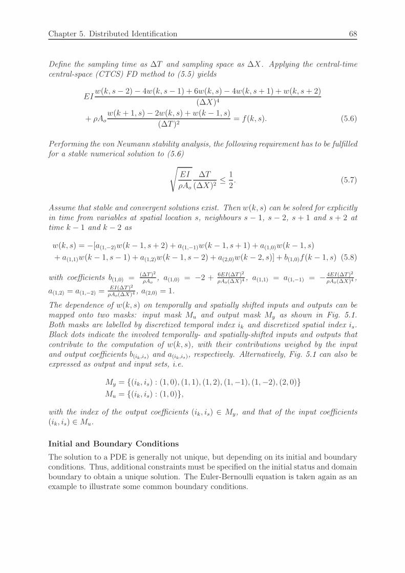
Chapter 5. Distributed Identification 68
Define the sampling time as ∆T and sampling space as ∆X. Applying the central-timecentral-space (CTCS) FD method to (5.5) yields
EIw(k, s− 2)− 4w(k, s− 1) + 6w(k, s)− 4w(k, s+ 1) + w(k, s+ 2)
(∆X)4
+ ρAo
w(k + 1, s)− 2w(k, s) + w(k − 1, s)
(∆T )2= f(k, s). (5.6)
Performing the von Neumann stability analysis, the following requirement has to be fulfilledfor a stable numerical solution to (5.6)
√
EI
ρAo
∆T
(∆X)2≤ 1
2. (5.7)
Assume that stable and convergent solutions exist. Then w(k, s) can be solved for explicitlyin time from variables at spatial location s, neighbours s − 1, s − 2, s + 1 and s + 2 attime k − 1 and k − 2 as
w(k, s) = −[a(1,−2)w(k − 1, s+ 2) + a(1,−1)w(k − 1, s+ 1) + a(1,0)w(k − 1, s)
+ a(1,1)w(k − 1, s− 1) + a(1,2)w(k − 1, s− 2) + a(2,0)w(k − 2, s)] + b(1,0)f(k − 1, s) (5.8)
with coefficients b(1,0) = (∆T )2
ρAo, a(1,0) = −2 + 6EI(∆T )2
ρAo(∆X)4, a(1,1) = a(1,−1) = − 4EI(∆T )2
ρAo(∆X)4,
a(1,2) = a(1,−2) =EI(∆T )2
ρAo(∆X)4, a(2,0) = 1.
The dependence of w(k, s) on temporally and spatially shifted inputs and outputs can bemapped onto two masks: input mask Mu and output mask My as shown in Fig. 5.1.Both masks are labelled by discretized temporal index ik and discretized spatial index is.Black dots indicate the involved temporally- and spatially-shifted inputs and outputs thatcontribute to the computation of w(k, s), with their contributions weighed by the inputand output coefficients b(ik ,is) and a(ik ,is), respectively. Alternatively, Fig. 5.1 can also beexpressed as output and input sets, i.e.
My = (ik, is) : (1, 0), (1, 1), (1, 2), (1,−1), (1,−2), (2, 0)Mu = (ik, is) : (1, 0),
with the index of the output coefficients (ik, is) ∈ My, and that of the input coefficients(ik, is) ∈ Mu.
Initial and Boundary Conditions
The solution to a PDE is generally not unique, but depending on its initial and boundaryconditions. Thus, additional constraints must be specified on the initial status and domainboundary to obtain a unique solution. The Euler-Bernoulli equation is taken again as anexample to illustrate some common boundary conditions.

Chapter 5. Distributed Identification 69
Mu isis
ikik
My
Figure 5.1: Input and output masks resulted from applying the CTCS FD method tosolve the Euler-Bernoulli equation
Example 5.2 (Common Boundary Conditions for the Euler-Bernoulli Equation)Denote the beam length as l. The boundary conditions for a free-free beam, where no re-striction is applied to the boundary subsystems, and for a beam with one clamped end aredefined as following:
• Free-free boundary condition at boundaries x = 0, l
EI∂2w(t, x)
∂x2|(x=0,l) = 0, EI
∂3w(t, x)
∂x3|(x=0,l) = 0. (5.9)
• Clamped at one end, e.g. x = 0
w(t, x)|(x=0) = 0,∂w(t, x)
∂x|(x=0) = 0. (5.10)
5.2.2 Two-Dimensional Input/Output Model Structure
Motivated by the two-dimensional difference equation (5.8), the lumped linear ARX model(4.4) has been extended to represent multidimensional systems in [27].
Define u(k, s) as the discrete input signal applied to a two-dimensional discrete SISOdata-generating system as shown in Fig. 5.2. The input/output dynamics of the plantmodel and the noise model take the form
A(qt, qs)y0(k, s) = B(qt, qs)u(k, s) (5.11)
A(qt, qs)v(k, s) = e(k, s), (5.12)
where e(k, s) represents a two-dimensional Gaussian white noise signal with zero mean,and v(k, s) the filtered noise.
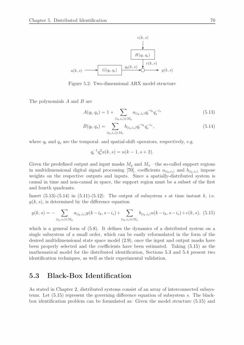
Chapter 5. Distributed Identification 70
u(k, s) G(qt, qs)y0(k, s)
e(k, s)
H(qt, qs)
v(k, s)
y(k, s)
Figure 5.2: Two-dimensional ARX model structure
The polynomials A and B are
A(qt, qs) = 1 +∑
(ik,is)∈My
a(ik ,is)q−ikt q−is
s (5.13)
B(qt, qs) =∑
(ik,is)∈Mu
b(ik ,is)q−ikt q−is
s , (5.14)
where qt and qs are the temporal- and spatial-shift operators, respectively, e.g.
q−1t q2su(k, s) = u(k − 1, s+ 2).
Given the predefined output and input masks My and Mu—the so-called support regionsin multidimensional digital signal processing [70], coefficients a(ik ,is) and b(ik ,is) imposeweights on the respective outputs and inputs. Since a spatially-distributed system iscausal in time and non-causal in space, the support region must be a subset of the firstand fourth quadrants.
Insert (5.13)-(5.14) in (5.11)-(5.12). The output of subsystem s at time instant k, i.e.y(k, s), is determined by the difference equation
y(k, s) = −∑
(ik ,is)∈My
a(ik ,is)y(k−ik, s−is)+∑
(ik ,is)∈Mu
b(ik ,is)u(k−ik, s−is)+e(k, s), (5.15)
which is a general form of (5.8). It defines the dynamics of a distributed system on asingle subsystem of a small order, which can be easily reformulated in the form of thedesired multidimensional state space model (2.9), once the input and output masks havebeen properly selected and the coefficients have been estimated. Taking (5.15) as themathematical model for the distributed identification, Sections 5.3 and 5.4 present twoidentification techniques, as well as their experimental validation.
5.3 Black-Box Identification
As stated in Chapter 2, distributed systems consist of an array of interconnected subsys-tems. Let (5.15) represent the governing difference equation of subsystem s. The black-box identification problem can be formulated as: Given the model structure (5.15) and

Chapter 5. Distributed Identification 71
measured input and output data sequences u(k, s), y(k, s), k = 1, . . . , Nk, s = 1, . . . , Ns,where Nk and Ns are the sizes of temporal and spatial measurements, respectively, find theproper input and output masks Mu and My, and estimate their corresponding coefficientsb(ik ,is) and a(ik ,is), such that the cost function
J =Ns∑
s=1
Nk∑
k=1
(y(k, s)− y(k, s))2 (5.16)
is minimized, where y(k, s) denotes the estimated output.
This section considers not only the identification of LTSI models, but also spatial LPVmodels for systems with spatially-varying features. In [27], the simplest least-squaresmethod is employed to identify a parametric model of an LTSI system. The identificationof a spatial LPV model is presented in [29] by extending the input/output identificationtechniques for temporal LPV systems. Accounting for the precence of colored noise,techniques for improved identification are developed in [71], [72] and [73]. This sectionfocuses on the application of the simplest least-squares based techniques developed in [27]and [29] for the identification of LTSI and spatial LPV models, respectively.
5.3.1 Identification of LTSI Models
LTSI models are used to represent distributed systems comprised of a number of identicalsubsystems, thus having identical coefficients a(ik ,is) and b(ik ,is) in (5.15) for all subsystems.
The input and output masks Mu and My are often unknown before the identificationprocedure is complete; they need to be updated by comparing various configurations.Provided an initial choice of the masks, the output can be estimated by rewriting thedifference equation (5.15) into regressor form as
y(k, s) = φT (k, s)p, (5.17)
where the parameter vector
p =
[[catikcatisa(ik,is)
]
(ik,is)∈My[catikcatisb(ik ,is)
]
(ik ,is)∈Mu
]
∈ Rnp (5.18)
contains unknown coefficients. The symbol catikcatis means the concatenation of coeffi-cients a(ik ,is) and b(ik ,is) with respect to ik and is as a vector, with (ik, is) subject to setsMy and Mu, respectively. In the Euler-Bernoulli equation example, we have
p = [a(1,−2), a(1,−1), a(1,0), a(1,1), a(1,2), a(2,0), b(1,0)]T . (5.19)
The data vector
φ(k, s) =
[[−catikcatisy(k − ik, s− is)
]
(ik,is)∈My[catikcatisu(k − ik, s− is)
]
(ik,is)∈Mu
]
∈ Rnφ (5.20)
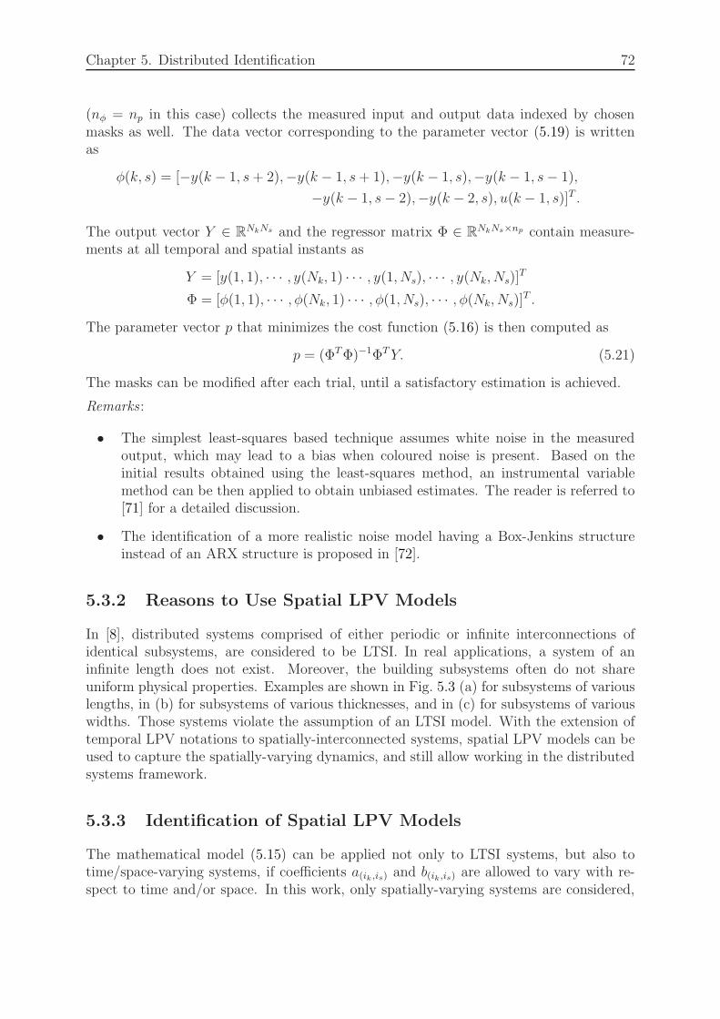
Chapter 5. Distributed Identification 72
(nφ = np in this case) collects the measured input and output data indexed by chosenmasks as well. The data vector corresponding to the parameter vector (5.19) is writtenas
φ(k, s) = [−y(k − 1, s+ 2),−y(k − 1, s+ 1),−y(k − 1, s),−y(k − 1, s− 1),
−y(k − 1, s− 2),−y(k − 2, s), u(k − 1, s)]T .
The output vector Y ∈ RNkNs and the regressor matrix Φ ∈ RNkNs×np contain measure-ments at all temporal and spatial instants as
Y = [y(1, 1), · · · , y(Nk, 1) · · · , y(1, Ns), · · · , y(Nk, Ns)]T
Φ = [φ(1, 1), · · · , φ(Nk, 1) · · · , φ(1, Ns), · · · , φ(Nk, Ns)]T .
The parameter vector p that minimizes the cost function (5.16) is then computed as
p = (ΦTΦ)−1ΦTY. (5.21)
The masks can be modified after each trial, until a satisfactory estimation is achieved.
Remarks :
• The simplest least-squares based technique assumes white noise in the measuredoutput, which may lead to a bias when coloured noise is present. Based on theinitial results obtained using the least-squares method, an instrumental variablemethod can be then applied to obtain unbiased estimates. The reader is referred to[71] for a detailed discussion.
• The identification of a more realistic noise model having a Box-Jenkins structureinstead of an ARX structure is proposed in [72].
5.3.2 Reasons to Use Spatial LPV Models
In [8], distributed systems comprised of either periodic or infinite interconnections ofidentical subsystems, are considered to be LTSI. In real applications, a system of aninfinite length does not exist. Moreover, the building subsystems often do not shareuniform physical properties. Examples are shown in Fig. 5.3 (a) for subsystems of variouslengths, in (b) for subsystems of various thicknesses, and in (c) for subsystems of variouswidths. Those systems violate the assumption of an LTSI model. With the extension oftemporal LPV notations to spatially-interconnected systems, spatial LPV models can beused to capture the spatially-varying dynamics, and still allow working in the distributedsystems framework.
5.3.3 Identification of Spatial LPV Models
The mathematical model (5.15) can be applied not only to LTSI systems, but also totime/space-varying systems, if coefficients a(ik ,is) and b(ik ,is) are allowed to vary with re-spect to time and/or space. In this work, only spatially-varying systems are considered,
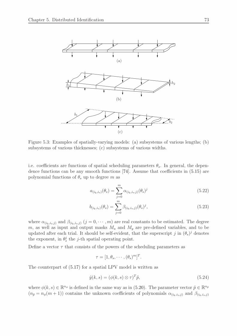
Chapter 5. Distributed Identification 73
h1h2
b1
b2
(a)
(b)
(c)
Figure 5.3: Examples of spatially-varying models: (a) subsystems of various lengths; (b)subsystems of various thicknesses; (c) subsystems of various widths.
i.e. coefficients are functions of spatial scheduling parameters θs. In general, the depen-dence functions can be any smooth functions [74]. Assume that coefficients in (5.15) arepolynomial functions of θs up to degree m as
a(ik,is)(θs) =m∑
j=0
α(ik,is,j)(θs)j (5.22)
b(ik ,is)(θs) =
m∑
j=0
β(ik,is,j)(θs)j, (5.23)
where α(ik ,is,j) and β(ik ,is,j) (j = 0, · · · , m) are real constants to be estimated. The degreem, as well as input and output masks Mu and My are pre-defined variables, and to beupdated after each trial. It should be self-evident, that the superscript j in (θs)
j denotesthe exponent, in θjs the j-th spatial operating point.
Define a vector τ that consists of the powers of the scheduling parameters as
τ = [1, θs, · · · , (θs)m]T .
The counterpart of (5.17) for a spatial LPV model is written as
y(k, s) = (φ(k, s)⊗ τ)T p, (5.24)
where φ(k, s) ∈ Rnφ is defined in the same way as in (5.20). The parameter vector p ∈ Rnp
(np = nφ(m+ 1)) contains the unknown coefficients of polynomials α(ik ,is,j) and β(ik ,is,j)
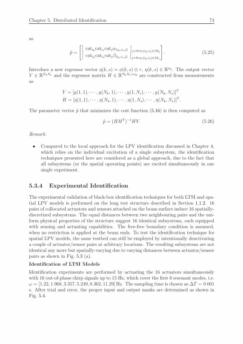
Chapter 5. Distributed Identification 74
as
p =
[[catikcatiscatjα(ik ,is,j)
]
j=0:m,(ik,is)∈My[catikcatiscatjβ(ik ,is,j)
]
j=0:m,(ik,is)∈Mu
]
. (5.25)
Introduce a new regressor vector η(k, s) = φ(k, s)⊗ τ , η(k, s) ∈ Rnp. The output vectorY ∈ RNkNs and the regressor matrix H ∈ RNkNs×np are constructed from measurementsas
Y = [y(1, 1), · · · , y(Nk, 1), · · · , y(1, Ns), · · · , y(Nk, Ns)]T
H = [η(1, 1), · · · , η(Nk, 1), · · · , η(1, Ns), · · · , η(Nk, Ns)]T .
The parameter vector p that minimizes the cost function (5.16) is then computed as
p = (HHT )−1HY. (5.26)
Remark:
• Compared to the local approach for the LPV identification discussed in Chapter 4,which relies on the individual excitation of a single subsystem, the identificationtechniques presented here are considered as a global approach, due to the fact thatall subsystems (or the spatial operating points) are excited simultaneously in onesingle experiment.
5.3.4 Experimental Identification
The experimental validation of black-box identification techniques for both LTSI and spa-tial LPV models is performed on the long test structure described in Section 1.1.2. 16pairs of collocated actuators and sensors attached on the beam surface induce 16 spatially-discretized subsystems. The equal distances between two neighbouring pairs and the uni-form physical properties of the structure suggest 16 identical subsystems, each equippedwith sensing and actuating capabilities. The free-free boundary condition is assumed,when no restriction is applied at the beam ends. To test the identification technique forspatial LPV models, the same testbed can still be employed by intentionally deactivatinga couple of actuator/sensor pairs at arbitrary locations. The resulting subsystems are notidentical any more but spatially-varying due to varying distances between actuator/sensorpairs as shown in Fig. 5.3 (a).
Identification of LTSI Models
Identification experiments are performed by actuating the 16 actuators simultaneouslywith 16 out-of-phase chirp signals up to 15 Hz, which cover the first 6 resonant modes, i.e.ω = [1.22, 1.968, 3.357, 5.249, 8.362, 11.29] Hz. The sampling time is chosen as ∆T = 0.001s. After trial and error, the proper input and output masks are determined as shown inFig. 5.4.
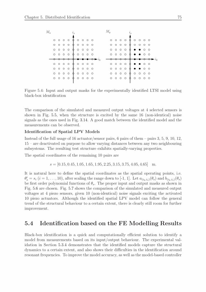
Chapter 5. Distributed Identification 75
Mu isis
ikik
My
Figure 5.4: Input and output masks for the experimentally identified LTSI model usingblack-box identification
The comparison of the simulated and measured output voltages at 4 selected sensors isshown in Fig. 5.5, when the structure is excited by the same 16 (non-identical) noisesignals as the ones used in Fig. 3.14. A good match between the identified model and themeasurements can be observed.
Identification of Spatial LPV Models
Instead of the full usage of 16 actuator/sensor pairs, 6 pairs of them – pairs 3, 5, 9, 10, 12,15 – are deactivated on purpose to allow varying distances between any two neighbouringsubsystems. The resulting test structure exhibits spatially-varying properties.
The spatial coordinates of the remaining 10 pairs are
s = [0.15, 0.45, 1.05, 1.65, 1.95, 2.25, 3.15, 3.75, 4.05, 4.65] m.
It is natural here to define the spatial coordinates as the spatial operating points, i.e.θis = si (i = 1, . . . , 10), after scaling the range down to [-1, 1]. Let a(ik,is)(θs) and b(ik ,is)(θs)be first order polynomial functions of θs. The proper input and output masks as shown inFig. 5.6 are chosen. Fig. 5.7 shows the comparison of the simulated and measured outputvoltages at 4 piezo sensors, given 10 (non-identical) noise signals exciting the activated10 piezo actuators. Although the identified spatial LPV model can follow the generaltrend of the structural behaviour to a certain extent, there is clearly still room for furtherimprovement.
5.4 Identification based on the FE Modelling Results
Black-box identification is a quick and computationally efficient solution to identify amodel from measurements based on its input/output behaviour. The experimental val-idation in Section 5.3.4 demonstrates that the identified models capture the structuraldynamics to a certain extent, and also shows their difficulties in the identification aroundresonant frequencies. To improve the model accuracy, as well as the model-based controller

Chapter 5. Distributed Identification 76
−1
0
1
−1
0
1
−1
0
1
30 30.5 31 31.5 32 32.5 33 33.5 34
−1
0
1
time (s)
outputvoltage(V
)
sensor 1
sensor 7
sensor 8
sensor 15
Figure 5.5: Comparison of the black-box simulated (blue) and measured (red) outputvoltages at 4 selected piezo sensors, given 16 (non-identical) noise signals exciting 16piezo actuators simultaneously.
Mu isis
ikik
My
Figure 5.6: Input and output masks for the experimentally identified spatial LPV modelusing black-box identification
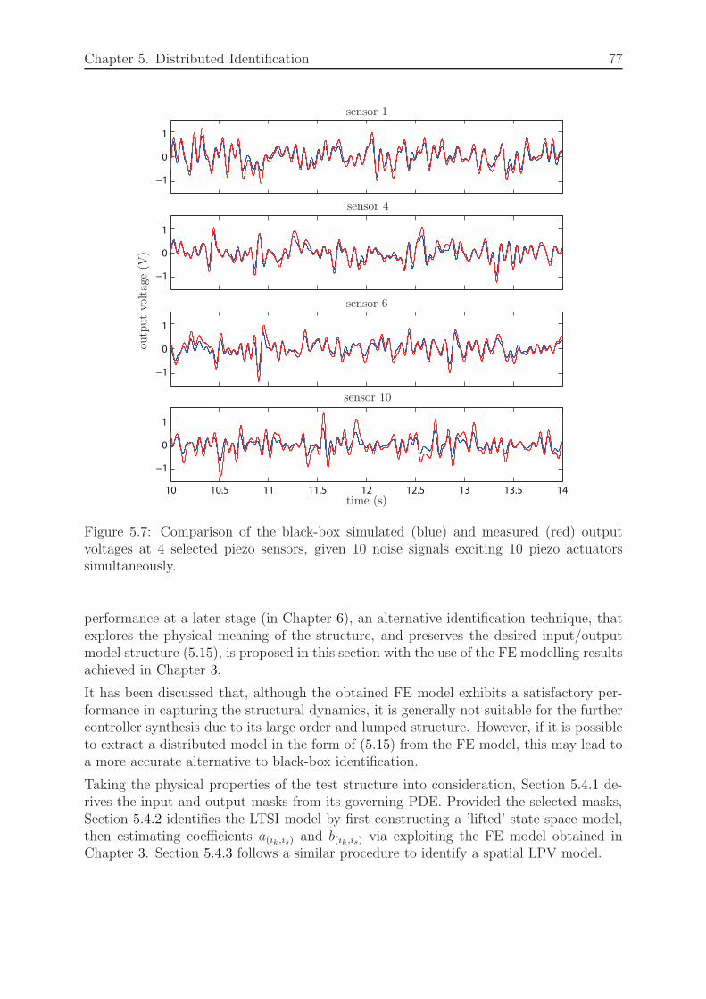
Chapter 5. Distributed Identification 77
−1
0
1
−1
0
1
−1
0
1
10 10.5 11 11.5 12 12.5 13 13.5 14
−1
0
1
time (s)
outputvoltage(V
)
sensor 1
sensor 4
sensor 6
sensor 10
Figure 5.7: Comparison of the black-box simulated (blue) and measured (red) outputvoltages at 4 selected piezo sensors, given 10 noise signals exciting 10 piezo actuatorssimultaneously.
performance at a later stage (in Chapter 6), an alternative identification technique, thatexplores the physical meaning of the structure, and preserves the desired input/outputmodel structure (5.15), is proposed in this section with the use of the FE modelling resultsachieved in Chapter 3.
It has been discussed that, although the obtained FE model exhibits a satisfactory per-formance in capturing the structural dynamics, it is generally not suitable for the furthercontroller synthesis due to its large order and lumped structure. However, if it is possibleto extract a distributed model in the form of (5.15) from the FE model, this may lead toa more accurate alternative to black-box identification.
Taking the physical properties of the test structure into consideration, Section 5.4.1 de-rives the input and output masks from its governing PDE. Provided the selected masks,Section 5.4.2 identifies the LTSI model by first constructing a ’lifted’ state space model,then estimating coefficients a(ik ,is) and b(ik ,is) via exploiting the FE model obtained inChapter 3. Section 5.4.3 follows a similar procedure to identify a spatial LPV model.

Chapter 5. Distributed Identification 78
5.4.1 PDE-Based Selection of Masks
The Euler-Bernoulli equation (5.5) establishes the linear relationship between externalforces and transverse displacements under Euler-Bernoulli beam theory. Recall the func-tionality of piezo patches as actuator and sensor described in Chapter 3: when the patchis used as an actuator, the input voltage is proportional to a pair of concentrated torquesapplied at the two electrode ends; as a sensor, the output voltage is proportional to thedifference of the slopes at the two electrode ends. Thus (5.5) can not be taken directly asthe governing PDE of the test structure. Nevertheless, it is possible to bring (5.5) into ashape that approximates this specific application.
First of all, the external force f(k, s) can be approximated by f ≈ M ′′p to bring the torque
into the PDE as
EI∂4w(t, x)
∂x4+ ρA
∂2w(t, x)
∂t2=
∂2Mp(t, x)
∂x2. (5.27)
Differentiating both sides of (5.27) twice with respect to x yields
EI∂4
∂x4(∂2w(t, x)
∂x2) + ρA
∂2
∂t2(∂2w(t, x)
∂x2) =
∂4Mp(t, x)
∂x4. (5.28)
Knowing that the second local derivative of the transverse displacement approximatesthe curvature κ, i.e. κ ≈ w′′, (5.28) can then be expressed with respect to torque andcurvature as
EI∂4κ(t, x)
∂x4+ ρA
∂2κ(t, x)
∂t2=
∂4Mp(t, x)
∂x4. (5.29)
Assume that the curvature κ approximates the difference of the slopes, when the distancebetween two electrode ends – in other words, the length of a piezo patch – is small
enough, i.e. κ ≈ w′′ ≈ w′
a−w′
b
xa−xb, where xa and xb are the x coordinates of the two electrode
boundaries a and b, respectively. Given the linear relationship between the output voltageφo and the difference of the slopes at the two electrode ends, i.e. φo = gs(w
′a − w′
b), φo isapproximately proportional to the curvature κ as well. Hence, a piezo pair of originallytwo nodes can be treated as a single node as shown in Fig. 5.8, where the input voltage φi
is proportional to the applied torque Mp, while the output voltage φo approximates thecurvature at the center of the electrodes.
M −M
w′a
w′b
φi
φo
Figure 5.8: Two electrode nodes are approximated by one node with a single input (inputvoltage) and single output (output voltage) at the center of the electrodes
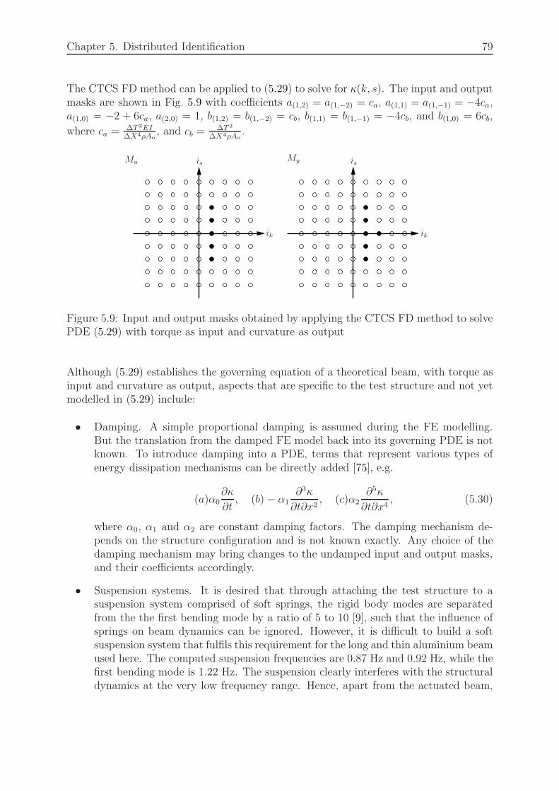
Chapter 5. Distributed Identification 79
The CTCS FD method can be applied to (5.29) to solve for κ(k, s). The input and outputmasks are shown in Fig. 5.9 with coefficients a(1,2) = a(1,−2) = ca, a(1,1) = a(1,−1) = −4ca,a(1,0) = −2 + 6ca, a(2,0) = 1, b(1,2) = b(1,−2) = cb, b(1,1) = b(1,−1) = −4cb, and b(1,0) = 6cb,
where ca =∆T 2EI∆X4ρAo
, and cb =∆T 2
∆X4ρAo.
Mu isis
ikik
My
Figure 5.9: Input and output masks obtained by applying the CTCS FD method to solvePDE (5.29) with torque as input and curvature as output
Although (5.29) establishes the governing equation of a theoretical beam, with torque asinput and curvature as output, aspects that are specific to the test structure and not yetmodelled in (5.29) include:
• Damping. A simple proportional damping is assumed during the FE modelling.But the translation from the damped FE model back into its governing PDE is notknown. To introduce damping into a PDE, terms that represent various types ofenergy dissipation mechanisms can be directly added [75], e.g.
(a)α0∂κ
∂t, (b)− α1
∂3κ
∂t∂x2, (c)α2
∂5κ
∂t∂x4, (5.30)
where α0, α1 and α2 are constant damping factors. The damping mechanism de-pends on the structure configuration and is not known exactly. Any choice of thedamping mechanism may bring changes to the undamped input and output masks,and their coefficients accordingly.
• Suspension systems. It is desired that through attaching the test structure to asuspension system comprised of soft springs, the rigid body modes are separatedfrom the the first bending mode by a ratio of 5 to 10 [9], such that the influence ofsprings on beam dynamics can be ignored. However, it is difficult to build a softsuspension system that fulfils this requirement for the long and thin aluminium beamused here. The computed suspension frequencies are 0.87 Hz and 0.92 Hz, while thefirst bending mode is 1.22 Hz. The suspension clearly interferes with the structuraldynamics at the very low frequency range. Hence, apart from the actuated beam,

Chapter 5. Distributed Identification 80
the suspension system becomes part of the structure to be modelled, which is notincluded in the theoretical PDE.
To account for the unaddressed issues, an enlarged output mask as shown in Fig. 5.10suggests a more complex model structure than Fig. 5.9. Both choices of masks in Fig. 5.9and Fig. 5.10 will be tested and compared for both the LTSI model and the spatial LPVmodel identification.
Mu isis
ikik
My
Figure 5.10: Input and (enlarged) output masks for the experimental identification
5.4.2 Identification of LTSI Models
With the input and output masks determined, coefficients a(ik ,is) and b(ik ,is) are constantsand identical for all subsystems just like black-box identification. Consider first the masksin Fig. 5.9 and assume a symmetric contribution from the left and the right neighbouringsubsystems, i.e. a1 = a(1,−2) = a(1,2), a2 = a(1,−1) = a(1,1), a3 = a(1,0), a4 = a(2,0),b1 = b(1,−2) = b(1,2), b2 = b(1,−1) = b(1,1), and b3 = b(1,0), where a1, a2, a3, a4, b1, b2, and b3are coefficients to be estimated. The difference equation in the form of (5.15) is expandedas
y(k, s) =− a1[y(k − 1, s− 2) + y(k − 1, s+ 2)]− a2[y(k − 1, s− 1) + y(k − 1, s+ 1)]
− a4[y(k − 2, s− 2) + y(k − 2, s+ 2)]− a5[y(k − 2, s− 1) + y(k − 2, s+ 1)]
+ b1[u(k − 1, s− 2) + u(k − 1, s+ 2)] + b2[u(k − 1, s− 1) + u(k − 1, s+ 1)]
− a3y(k − 1, s)− a6y(k − 2, s) + b3u(k − 1, s). (5.31)
To estimate the unknown coefficients, the FE model obtained in Chapter 3 is involved inthe identification procedure as follows:
1. Construct a ’lifted’ system. Given the difference equation (5.31), a state space model
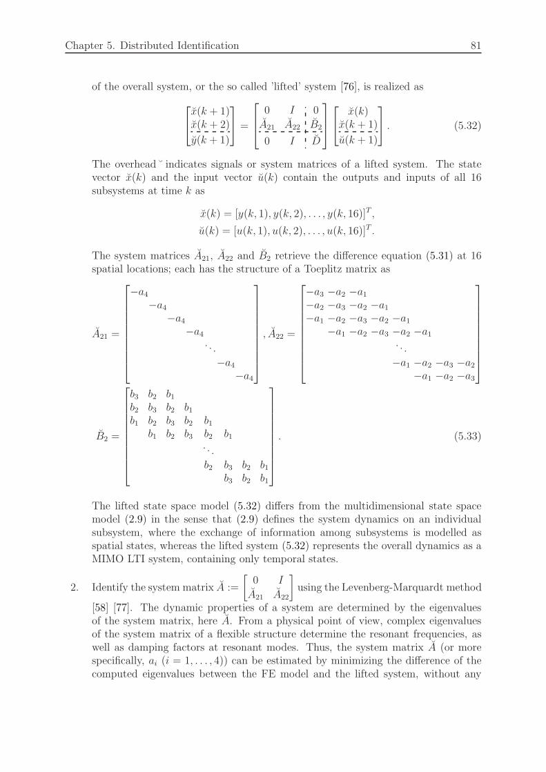
Chapter 5. Distributed Identification 81
of the overall system, or the so called ’lifted’ system [76], is realized as
x(k + 1)x(k + 2)
y(k + 1)
=
0 I 0
A21 A22 B2
0 I D
x(k)x(k + 1)
u(k + 1)
. (5.32)
The overhead ˘ indicates signals or system matrices of a lifted system. The statevector x(k) and the input vector u(k) contain the outputs and inputs of all 16subsystems at time k as
x(k) = [y(k, 1), y(k, 2), . . . , y(k, 16)]T ,
u(k) = [u(k, 1), u(k, 2), . . . , u(k, 16)]T .
The system matrices A21, A22 and B2 retrieve the difference equation (5.31) at 16spatial locations; each has the structure of a Toeplitz matrix as
A21 =
−a4−a4
−a4−a4
. . .
−a4−a4
, A22 =
−a3 −a2 −a1−a2 −a3 −a2 −a1−a1 −a2 −a3 −a2 −a1
−a1 −a2 −a3 −a2 −a1. . .
−a1 −a2 −a3 −a2−a1 −a2 −a3
B2 =
b3 b2 b1b2 b3 b2 b1b1 b2 b3 b2 b1
b1 b2 b3 b2 b1. . .
b2 b3 b2 b1b3 b2 b1
. (5.33)
The lifted state space model (5.32) differs from the multidimensional state spacemodel (2.9) in the sense that (2.9) defines the system dynamics on an individualsubsystem, where the exchange of information among subsystems is modelled asspatial states, whereas the lifted system (5.32) represents the overall dynamics as aMIMO LTI system, containing only temporal states.
2. Identify the system matrix A :=
[0 I
A21 A22
]
using the Levenberg-Marquardt method
[58] [77]. The dynamic properties of a system are determined by the eigenvaluesof the system matrix, here A. From a physical point of view, complex eigenvaluesof the system matrix of a flexible structure determine the resonant frequencies, aswell as damping factors at resonant modes. Thus, the system matrix A (or morespecifically, ai (i = 1, . . . , 4)) can be estimated by minimizing the difference of thecomputed eigenvalues between the FE model and the lifted system, without any
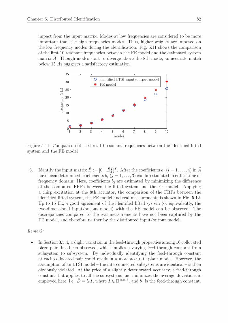
Chapter 5. Distributed Identification 82
impact from the input matrix. Modes at low frequencies are considered to be moreimportant than the high frequencies modes. Thus, higher weights are imposed onthe low frequency modes during the identification. Fig. 5.11 shows the comparisonof the first 10 resonant frequencies between the FE model and the estimated systemmatrix A. Though modes start to diverge above the 8th mode, an accurate matchbelow 15 Hz suggests a satisfactory estimation.
1 2 3 4 5 6 7 8 9 100
5
10
15
20
25
30
35
modes
frequency
(Hz)
identified LTSI input/output model
FE model
Figure 5.11: Comparison of the first 10 resonant frequencies between the identified liftedsystem and the FE model
3. Identify the input matrix B := [0 BT2 ]
T . After the coefficients ai (i = 1, . . . , 4) in Ahave been determined, coefficients bj (j = 1, . . . , 3) can be estimated in either time orfrequency domain. Here, coefficients bj are estimated by minimizing the differenceof the computed FRFs between the lifted system and the FE model. Applyinga chirp excitation at the 8th actuator, the comparison of the FRFs between theidentified lifted system, the FE model and real measurements is shown in Fig. 5.12.Up to 15 Hz, a good agreement of the identified lifted system (or equivalently, thetwo-dimensional input/output model) with the FE model can be observed. Thediscrepancies compared to the real measurements have not been captured by theFE model, and therefore neither by the distributed input/output model.
Remark:
• In Section 3.5.4, a slight variation in the feed-through properties among 16 collocatedpiezo pairs has been observed, which implies a varying feed-through constant fromsubsystem to subsystem. By individually identifying the feed-through constantat each collocated pair could result in a more accurate plant model. However, theassumption of an LTSI model – the interconnected subsystems are identical – is thenobviously violated. At the price of a slightly deteriorated accuracy, a feed-throughconstant that applies to all the subsystems and minimizes the average deviations isemployed here, i.e. D = b0I, where I ∈ R16×16, and b0 is the feed-through constant.
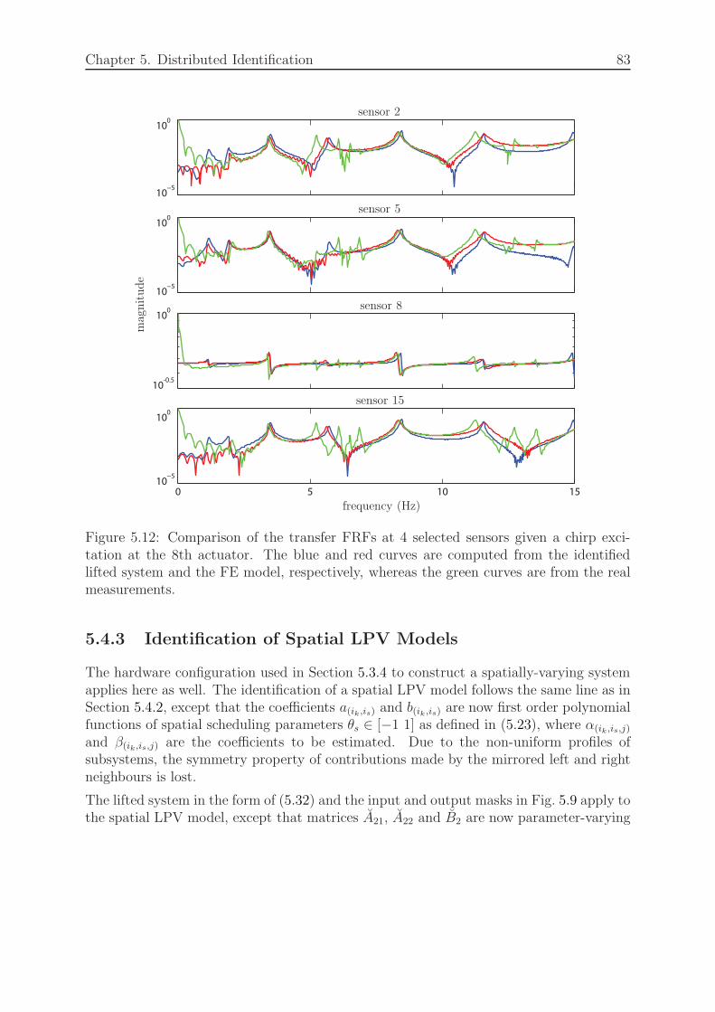
Chapter 5. Distributed Identification 83
10−5
100
10−5
100
100
0 5 10 15
10−5
100
10-0.5
frequency (Hz)
magnitude
sensor 2
sensor 5
sensor 8
sensor 15
Figure 5.12: Comparison of the transfer FRFs at 4 selected sensors given a chirp exci-tation at the 8th actuator. The blue and red curves are computed from the identifiedlifted system and the FE model, respectively, whereas the green curves are from the realmeasurements.
5.4.3 Identification of Spatial LPV Models
The hardware configuration used in Section 5.3.4 to construct a spatially-varying systemapplies here as well. The identification of a spatial LPV model follows the same line as inSection 5.4.2, except that the coefficients a(ik ,is) and b(ik ,is) are now first order polynomialfunctions of spatial scheduling parameters θs ∈ [−1 1] as defined in (5.23), where α(ik ,is,j)
and β(ik,is,j) are the coefficients to be estimated. Due to the non-uniform profiles ofsubsystems, the symmetry property of contributions made by the mirrored left and rightneighbours is lost.
The lifted system in the form of (5.32) and the input and output masks in Fig. 5.9 apply tothe spatial LPV model, except that matrices A21, A22 and B2 are now parameter-varying

Chapter 5. Distributed Identification 84
and constructed as
A21(θs) =
−a(2,0)(θ1s)−a(2,0)(θ
2s)−a(2,0)(θ
3s). . .
−a(2,0)(θ10s )
A22(θs) =
−a(1,0)(θ1s) −a(1,−1)(θ
1s) −a(1,−2)(θ
1s)
−a(1,1)(θ2s) −a(1,0)(θ
2s) −a(1,−1)(θ
2s) −a(1,−2)(θ
2s)
−a(1,2)(θ3s) −a(1,1)(θ
3s) −a(1,0)(θ
3s) −a(1,−1)(θ
3s) −a(1,−2)(θ
3s)
. . .
−a(1,2)(θ10s ) −a(1,1)(θ
10s ) −a(1,0)(θ
10s )
B2(θs) =
b(1,0)(θ1s) b(1,−1)(θ
1s) b(1,−2)(θ
1s)
b(1,1)(θ2s) b(1,0)(θ
2s) b(1,−1)(θ
2s) b(1,−2)(θ
2s)
b(1,2)(θ3s) b(1,1)(θ
3s) b(1,0)(θ
3s) b(1,−1)(θ
3s) b(1,−2)(θ
3s)
. . .
b(1,2)(θ10s ) b(1,1)(θ
10s ) b(1,0)(θ
10s )
.
Although the hardware is reconfigured compared to the LTSI model—10 instead of 16actuator/sensor pairs are actually activated, the test structure itself – the aluminiumbeam – remain unchanged, and so do the eigenvalues. The system matrix A can still beestimated by minimizing the difference of computed eigenvalues between the identifiedlifted system and the FE model.
Fig. 5.13 shows the comparison of the computed resonant frequencies between the identi-fied LPV model and the FE model. An even better match than in Fig. 5.11 for an LTSImodel identification has been achieved. This may be due to the fact that the introductionof more decision variables provides extra degrees of freedom in the estimation. After theB matrix being estimated, Fig. 5.14 is generated in the same way as Fig. 5.7. It canbe easily seen, that the discrepancies between the simulated and measured subsystemresponses in Fig. 5.14 are considerably reduced compared to Fig. 5.7.
Remarks:
• Similar procedures have been applied to identify more complex LTSI and spatialLPV models, by employing the enlarged masks in Fig. 5.10. The identificationresults do not show a significant improvement compared to the identified modelsusing the masks in Fig. 5.9. Keep in mind that the identified models will be usedfor model-based controller design. Models of smaller sizes are therefore preferred.
• Under the assumption that the governing PDE of a spatially-distributed system isnot known accurately, yet its FE model is available (which is realistic, because FEmodelling has become a routine process in structural engineering for the analysisof test structures for decades), the proposed identification procedures fill the gap

Chapter 5. Distributed Identification 85
1 2 3 4 5 6 7 8 9 100
5
10
15
20
25
30
35
modes
frequency
(Hz)
identified LPV input/output model
FE model
Figure 5.13: Comparison of the first 10 resonant frequencies between the identified LPVmodel and the FE model
−1
0
1
−1
0
1
−1
0
1
10 10.5 11 11.5 12 12.5 13 13.5 14
−1
0
1
time (s)
outputvoltage(V
)
sensor 1
sensor 4
sensor 6
sensor 10
Figure 5.14: Comparison of the FE-based simulated (blue) and measured (red) outputvoltages at 4 selected piezo sensors, given 10 noise signals exciting 10 piezo actuatorssimultaneously.

Chapter 5. Distributed Identification 86
between the FE modelling and distributed identification by extracting distributedmodels from the FE model.
• The identified input/output models are subject to the accuracy of the FE model.Structural dynamics which are not captured by the FE modelling can not be takencare of by the input/output model either.
5.5 Summary
This chapter has dealt with the distributed identification of both LTSI and spatial LPVmodels. A two-dimensional input/output model derived by applying the FD method tothe governing PDE of a beam structure – the Euler-Bernoulli equation – defines the struc-tural dynamics on spatially-discretized subsystems, and preserves the distributed natureof the flexible structure. Its general form is determined as the mathematical model for thedistributed identification. The two-dimensional black-box identification techniques havebeen briefly reviewed and implemented on the test structure. The experimental validationdemonstrated that the identified models represent the structural dynamics to a certainextent, but also display their difficulties in capturing the dynamics around resonant fre-quencies. For this reason, alternative identification procedures have been proposed byextracting distributed models from the FE model, with the desired model structure stillmaintained. Using the proposed procedures, a considerably improved agreement betweenmeasurements and identified models has been achieved in the experimental implementa-tion.

Chapter 6
Distributed Controller Design
6.1 Introduction
This chapter deals with the controller design for both parameter-invariant and parameter-varying distributed systems. In many cases, a centralized controller fails to efficientlycontrol a distributed system due to a high level of connectivity and computational bur-den caused by a large number of inputs and outputs. By inheriting the interconnectedstructure of the plant, distributed controller design at the subsystem level is much easierto handle.
In the last decade, distributed controller design has been studied by various researchersfrom different perspectives. A novel multidimensional state space framework, that ad-dresses the system analysis and controller synthesis problem based on a single subsystem,has been proposed in [8]. Employing the state space model developed in [8], [30] takes adifferent path by solving the controller design problem of a ’lifted’ system, which describesthe overall dynamics by augmenting subsystems, using a sequentially semi-separable ap-proach. Iterative algorithms are employed for a sub-optimal controller synthesis. Adecomposition approach is proposed in [31] for interconnected systems, if the system ma-trices of these systems satisfy a certain structural property. Then it is possible to designa distributed controller which has the same interconnected pattern as the plant. Basedon two-dimensional loop shaping concepts, [32] solves the controller design problem ofa typical industrial spatially-distributed system – the papermaking machine – throughdecoupling the large-scale multi-variable system into a family of SISO design problems,one at each spatial frequency. In [78], an efficient and computationally tractable de-sign method to optimize the design parameters of both the plant and the controller in acollocated structural system has been proposed using a norm upper bound approach.
In this work, the controller design problem is addressed in the framework developed in[8]. Given the experimentally identified input/output models in Chapter 5, their multidi-mensional state space representations are realized first. Analysis and synthesis conditionsfor the design of both distributed and decentralized controllers for LTSI systems are pro-vided. The LPV control technique for lumped systems has been extended to addressspatio-temporal systems in [21] using CLFs, under the assumption of an LFT-based de-
87
Chapter 6. Distributed Controller Design 88
pendence of the state space model on scheduling parameters. To reduce the conservatismincurred by the use of CLFs for parameter-varying systems with bounded variation rates,analysis and synthesis conditions using PDLFs for lumped systems are extended hereto parameter-varying distributed systems. Experimental results validate the controllerperformance in terms of output disturbance rejection.
This chapter includes results reported in [79] and [80]. It is organized as follows: Section6.2 converts the identified LTSI and spatial LPV input/output models into their statespace representations. Section 6.3 presents a procedure for the construction of multidi-mensional generalized plants. Synthesis conditions for LTSI distributed controllers devel-oped in [8] are recapped in Section 6.4, whereas conditions for decentralized controllerdesign are provided in Section 6.4.2, with their performance evaluated experimentally inSection 6.4.3. The LPV controller design for time/space-varying systems is discussed inSection 6.5. Conditions for distributed LPV controller design using CLFs – less conser-vative than [21] – are given in Section 6.5.1. To further reduce the conservatism whenan upper bound on the variation rate of scheduling parameters is known, the LPV con-trol technique using PDLFs is extended from lumped systems to distributed systems inSection 6.5.2. Experimental results of closed-loop systems with controllers designed usingboth CLFs and PDLFs are demonstrated in Section 6.5.3.
6.2 Multidimensional State Space Realization
It has been justified in Chapter 5, that the test structure considered in this work canbe described using a two-dimensional input/output model. A model-based controller caneither be designed in input/output form of a fixed structure ([81], [82]), or in a state spaceframework. In this work, system analysis and controller synthesis are realized in statespace framework. In order to apply the state-space based synthesis tools developed in[8], the realization of the identified input/output models into their multidimensional statespace representations in the form of (2.9) is first required. The simple Euler-Bernoulliequation in Example 5.1 is used as an example here to illustrate the general proceduresin multidimensional state space realization.
Example 6.1 (State Space Realization of the Euler-Bernoulli Equation) Afterapplying the FD method, the solution of the PDE (5.5) can be approximated by the dif-ference equation (5.6). It states that the output of subsystem s at time k – y(k, s) – isdetermined by the outputs of itself at time k − 1 and k − 2, the outputs of its neighbourss− 2, s− 1, s+ 1 and s+ 2 at time k − 1, and its own input at k − 1.
Follow the routines of constructing a lumped state space model in controller canonicalform. Define the transverse displacement as output y(k, s) = w(k, s), and the appliedforce as input u(k, s) = f(k, s). The difference equation implies its transfer functionmodel
Y
U=B(qt, qs)
A(qt, qs)=
b(1,0)qt
q2t + a(1,−2)qtq2s + a(1,−1)qtqs + a(1,0)qt + a(1,1)qtq−1s + a(1,2)qtq−2
s + a(2,0).
(6.1)

Chapter 6. Distributed Controller Design 89
Define a new variable V (qt, qs), such that
U = AV, Y = BV, (6.2)
where U = AV yields the input equation
v(k + 2, s) =− a(1,−2)v(k + 1, s+ 2)− a(1,−1)v(k + 1, s+ 1)− a(1,0)v(k + 1, s)
− a(1,1)v(k + 1, s− 1)− a(1,2)v(k + 1, s− 2)− a(2,0)v(k, s) + u(k, s),
and Y = BV the output equation
y(k, s) = b(1,0)v(k + 1, s).
Let the temporal state, and the positive and negative spatial state vectors be selected as
xt =
[v(k, s)
v(k + 1, s)
]
x+s =
[v(k + 1, s− 2)v(k + 1, s− 1)
]
x−s =
[v(k + 1, s+ 2)v(k + 1, s+ 1)
]
, (6.3)
respectively. The multidimensional state space model in controller canonical form is real-ized as
xt(k + 1, s)x+s (k, s+ 1)
x−s (k, s− 1)
y(k, s)
=
0 1 0 0 0 0 0−a(2,0) −a(1,0) −a(1,2) −a(1,1) −a(1,−2) −a(1,−1) 1
0 0 0 1 0 0 00 1 0 0 0 0 00 0 0 0 0 1 00 1 0 0 0 0 0
0 b(1,0) 0 0 0 0 0
xt(k, s)x+s (k, s)
x−s (k, s)
u(k, s)
. (6.4)
Although the experimentally identified input/output models exhibit more complex dy-namics than the simple Euler-Bernoulli equation, the realization of their state space mod-els follows the similar line. The rest of this section converts the identified LTSI andspatial LPV models into their state space representations, considering models obtainedusing both black-box identification and the FE modelling results.
6.2.1 LTSI Models
The experimentally identified black-box LTSI model has the input and output masksshown in Fig. 5.4. Compared to the Euler-Bernoulli equation, the output of subsystems at time k, y(k, s), additionally depends on the outputs of its neighbours at k − 2 andits own input at k − 2 and k − 3. Thus define the temporal state, positive and negativespatial state vector as
xt =
v(k, s)v(k + 1, s)v(k + 2, s)
x+s =
v(k + 1, s− 2)v(k + 1, s− 1)v(k + 2, s− 2)v(k + 2, s− 1)
x−s =
v(k + 1, s+ 2)v(k + 1, s+ 1)v(k + 2, s+ 2)v(k + 2, s+ 1)
, (6.5)
Chapter 6. Distributed Controller Design 90
respectively. A state space realization of the LTSI model takes the form
xt(k + 1, s)x+s (k, s+ 1)
x−s (k, s− 1)
y(k, s)
=
[
AG BG
CG DG
]
xt(k, s)x+s (k, s)
x−s (k, s)
u(k, s)
, (6.6)
with the system matrices given in Appendix (A.2) which are identical for all subsystems.
On the other hand, the FE-based LTSI model identified in Section 5.4 is endowed withphysical meanings, and governed by the input and output masks shown in Fig. 5.9, wherethe output y(k, s) depends on the past inputs applied on s, as well as on its neighbourss− 2, s− 1, s+ 1 and s+ 2. More intuitively, the black-box identified subsystem modelinteracts with nearby subsystems only through outputs, yet the FE-based model throughboth outputs and inputs. Thus the temporal state, positive and negative spatial statevectors are defined as
xt =
[v(k, s)
v(k + 1, s)
]
x+s =
v(k + 1, s− 2)v(k + 1, s− 1)u(k + 1, s− 2)u(k + 1, s− 1)
x−s =
v(k + 1, s+ 2)v(k + 1, s+ 1)u(k + 1, s+ 2)u(k + 1, s+ 1)
, (6.7)
respectively. Its state space realization takes the form of (6.6), with the system matricesexpressed in Appendix (A.3).
6.2.2 Spatial LPV Models
Consider first the black-box identified spatial LPV model. Provided the input and outputmasks shown in Fig. 5.6, the application of the multidimensional Z-transformation to theLPV difference equation yields
Y
U=B(θs, qt, qs)
A(θs, qt, qs)=
b(1,0)(θs)qt + b(2,0)(θs)
q2t + a(1,−2)(θs)qtq2s + a(1,−1)(θs)qtqs + a(1,0)(θs)qt + . . .+ a(2,2)(θs)q−2s
.
(6.8)Compared to (6.1), the coefficients in (6.8) are not identical for all subsystems any more;instead they are varying from subsystem to subsystem. Black-box identification performedin Section 5.3.3 suggests that all coefficients in (6.8) are first order polynomials of thespatial scheduling parameter θs ∈ R.
Again introduce a new variable V such that U = AV and Y = BV hold. The differenceequation of U = AV takes the form
v(k + 2, s) =− a(1,−2)(θs)v(k + 1, s+ 2)− a(1,−1)(θs)v(k + 1, s+ 1)− a(1,0)(θs)v(k + 1, s)
− a(1,1)(θs)v(k + 1, s− 1)− . . .− a(2,2)(θs)v(k, s− 2) + u(k, s)
=−(α(1,−2,0)+α(1,−2,1)θs)v(k + 1, s+ 2)−(α(1,−1,0)+α(1,−1,1)θs)v(k + 1, s+ 1)
− (α(1,0,0) + α(1,0,1)θs)v(k + 1, s)− (α(1,1,0) + α(1,1,1)θs)v(k + 1, s− 1)
− (α(2,2,0) + α(2,2,1)θs)v(k, s− 2) + u(k, s). (6.9)
Chapter 6. Distributed Controller Design 91
Rearrange (6.9) by grouping all parameter-dependent terms together
v(k + 2, s) = −α(1,−2,0)v(k + 1, s+ 2)− α(1,−1,0)v(k + 1, s+ 1)− α(1,0,0)v(k + 1, s)
−α(1,1,0)v(k + 1, s− 1)− . . .− α(2,2,0)v(k, s− 2) + u(k, s) + ps1(k, s),
where
ps1(k, s) = θs[−α(1,−2,0)v(k + 1, s+ 2)− α(1,−1,0)v(k + 1, s+ 1)− α(1,0,0)v(k + 1, s)
− α(1,1,0)v(k + 1, s− 1)− . . .− α(2,2,0)v(k, s− 2)]
= θsqs1(k, s). (6.10)
Likewise, the difference equation of the output equation Y = BV is written as
y(k, s) = β(1,0,0)v(k + 1, s) + β(2,0,0)v(k, s) + ps2(k, s), (6.11)
where
ps2(k, s) = θs[β(1,0,1)v(k + 1, s) + β(2,0,1)v(k, s)]
= θsqs2(k, s). (6.12)
By pulling out the spatial uncertainties, the spatial LPV model can be represented inLFT form as shown in Fig. 6.1, which is a special case of the time/space-varying systemshown in Fig. 2.3. Its LFT LPV state space model is given by
xt(k + 1, s)x+s (k, s+ 1)
x−s (k, s− 1)
qs(k, s)
y(k, s)
=
AG BGp BG
u
CGq DG
qp DGqu
CGy DG
yp DGyu
xt(k, s)x+s (k, s)
x−s (k, s)
ps(k, s)
u(k, s)
, (6.13)
with the choices of vectors
xt =
[v(k, s)
v(k + 1, s)
]
x+s =
v(k, s− 2)v(k, s− 1)
v(k + 1, s− 2)v(k + 1, s− 1)
x−s =
v(k, s+ 2)v(k, s+ 1)
v(k + 1, s+ 2)v(k + 1, s+ 1)
, (6.14)
and the performance channel ps(k, s) =
[ps1(k, s)ps2(k, s)
]
, qs(k, s) =
[qs1(k, s)qs2(k, s)
]
, with
ps(k, s) =
[θs
θs
]
qs(k, s) = Θsqs(k, s). (6.15)
The system matrices of (6.13) can be found in Appendix (A.6).
The explicit LPV form of the LFT LPV model (6.13) and (6.15) can be written as
xt(k + 1, s)x+s (k, s+ 1)
x−s (k, s− 1)
y(k, s)
=
[
AG(Θs) BGu (Θs)
CGy (Θs) DG
yu(Θs)
]
xt(k, s)x+s (k, s)
x−s (k, s)
u(k, s)
, (6.16)

Chapter 6. Distributed Controller Design 92
GG G
Θs−1 Θs Θs+1
ps(k, s−1) qs(k, s−1) ps(k, s) qs(k, s) ps(k, s+1) qs(k, s+1)
Figure 6.1: Spatially-varying distributed system in LFT representation
where the system matrices are scheduled by the structured spatial uncertainty Θs ∈ R2×2,and can be recovered from (6.13) and (6.15) as
[AG(Θs) BGu (Θs)
CGy (Θs) DG
yu(Θs)
]
=
[AG BG
u
CGy DG
yu
]
+
[BG
p
DGyp
]
Θs(I −DGqpΘs)
[CG
q DGqu
]. (6.17)
Analogous to the state space realization of the black-box identified spatial LPV model, theFE-based spatial LPV model identified in Section 5.4.3 has a state space representationgiven in Appendix (A.7) with the same choice of the states as in (6.7).
Remarks :
• It is demonstrated in [83] that, when converting a lumped LPV input/output modelinto a state space representation, the phenomenon of dynamic dependence arises: theresulting state space model depends on time-shifted versions of scheduling parame-ters. This phenomenon may also occur when converting a spatial LPV input/outputmodel into state space form, where the resulting state space model depends on space-shifted scheduling parameters. To explore the property of dynamic dependence ina distributed LPV model, consider the observer canonical form of (6.16), whoseoutput equation is expressed as y(k, s) = xt(k, s), and
y(k, s) = AGtt(Θs)xt(k − 1, s) +AG,+
ts (Θs)x+s (k − 1, s) +AG,−
ts (Θs)xG,−s (k − 1, s)
+ BGt,u(Θs)u(k, s). (6.18)
Replace x+s (k − 1, s) and x−
s (k − 1, s) in (6.18) with
x+s (k − 1, s) = AG,+
st (Θs−1)xt(k − 1, s− 1) +AG,++ss (Θs−1)x
+s (k − 1, s− 1)
+AG,+−ss (Θs−1)x
−s (k − 1, s− 1) + BG,+
s,u (Θs)u(k − 1, s)
x−s (k − 1, s) = AG,−
st (Θs+1)xt(k − 1, s+ 1) +AG,−+ss (Θs+1)x
+s (k − 1, s+ 1)
+AG,−−ss (Θs+1)x
−s (k − 1, s+ 1) + BG,−
s,u (Θs)u(k − 1, s).
The computation of y(k, s) depends on the scheduling parameter at s, i.e. Θs, aswell as on the space-shifted scheduling parameters at s− 1 and s+1, i.e. Θs−1 and

Chapter 6. Distributed Controller Design 93
Θs+1. That is the so-called dynamic dependence. However, this issue arises onlywhen the block matrix
[
AG,+st (Θs) AG,++
ss (Θs) AG,+−ss (Θs) BG,+
s,u (Θs)
AG,−st (Θs) AG,−+
ss (Θs) AG,−−ss (Θs) BG,−
s,u (Θs)
]
(6.19)
is gain-scheduled.
Recall the state space realization (6.4) of an LTSI model. An explicit LPV form ofthe spatial LPV model (6.16) can be constructed following the same pattern, whereparameter-dependent coefficients a(ik ,is)(θs) and b(ik ,is)(θs) appear only in block ma-
trices
[
AGtt(Θs) AG,+
ts (Θs) AG,−ts (Θs) BG
t,u(Θs)
CG,t,y(Θs) CG,+
s,y (Θs) CG,−s,y (Θs) DG
yu(Θs)
]
, leaving the block matrix (6.19) in
(6.16) consisting of static terms—0 and 1, which indicate the signal flow betweensubsystems. Therefore, the phenomenon of dynamic dependence is not an issue inthis specific application. The equivalence between the input/output LPV modeland the converted state space model is not affected.
• The equivalence between the identified input/output model and the transformedmultidimensional state space model has been validated by comparing their open-loop responses.
6.3 Construction of a Generalized Plant
The goal of designing a controller is to exponentially stabilize the controlled system andto impose a performance specification from the generalized disturbance w, which couldbe a combination of an input disturbance d, output noise n and reference input r, to thefictitious controlled variable z, which measures the controller satisfying certain properties,e.g. with regard to the control error e, and the control effort u [84]. The construction of ageneralized plant for distributed systems does not differ much from lumped systems, ex-cept that the performance weightings can be either defined as multidimensional, involvingboth temporal and spatial dynamics, or purely temporal.
Note that a multidimensional weighting filter itself is a spatially-interconnected system.Although the two-dimensional loop shaping problem has been considered in [85] for acirculant system, how to construct and parametrize a multidimensional filter to specifycertain performance requirements on a controlled distributed system is not known. Thus,one-dimensional temporal weighting filters are tuned and incorporated here in the spatio-temporal generalized plant.
Let the disturbance d(k, s) be injected into the output of subsystem s as shown in Fig. 6.2.Considered here is a controller design by shaping the mixed sensitivities: sensitivity tosuppress the output disturbance, and control sensitivity to impose an upper bound on thecontrol effort. The weighting filter WK used to shape the control sensitivity has a state
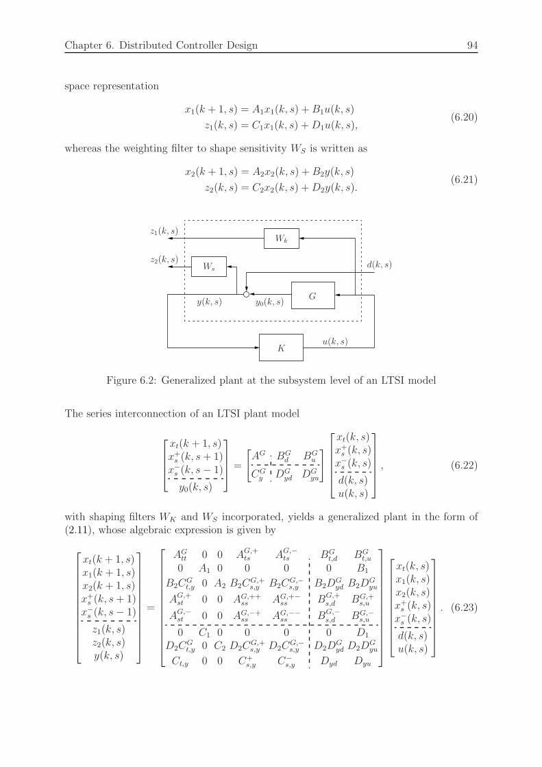
Chapter 6. Distributed Controller Design 94
space representation
x1(k + 1, s) = A1x1(k, s) +B1u(k, s)
z1(k, s) = C1x1(k, s) +D1u(k, s),(6.20)
whereas the weighting filter to shape sensitivity WS is written as
x2(k + 1, s) = A2x2(k, s) +B2y(k, s)
z2(k, s) = C2x2(k, s) +D2y(k, s).(6.21)
G
K
Wk
Wsd(k, s)
z1(k, s)
z2(k, s)
u(k, s)
y0(k, s)y(k, s)
Figure 6.2: Generalized plant at the subsystem level of an LTSI model
The series interconnection of an LTSI plant model
xt(k + 1, s)x+s (k, s+ 1)
x−s (k, s− 1)
y0(k, s)
=
[
AG BGd BG
u
CGy DG
yd DGyu
]
xt(k, s)x+s (k, s)
x−s (k, s)
d(k, s)u(k, s)
, (6.22)
with shaping filters WK and WS incorporated, yields a generalized plant in the form of(2.11), whose algebraic expression is given by
xt(k + 1, s)x1(k + 1, s)x2(k + 1, s)x+s (k, s+ 1)
x−s (k, s− 1)
z1(k, s)z2(k, s)y(k, s)
=
AGtt 0 0 AG,+
ts AG,−ts BG
t,d BGt,u
0 A1 0 0 0 0 B1
B2CGt,y 0 A2 B2C
G,+s,y B2C
G,−s,y B2D
Gyd B2D
Gyu
AG,+st 0 0 AG,++
ss AG,+−ss BG,+
s,d BG,+s,u
AG,−st 0 0 AG,−+
ss AG,−−ss BG,−
s,d BG,−s,u
0 C1 0 0 0 0 D1
D2CGt,y 0 C2 D2C
G,+s,y D2C
G,−s,y D2D
Gyd D2D
Gyu
Ct,y 0 0 C+s,y C−
s,y Dyd Dyu
xt(k, s)x1(k, s)x2(k, s)x+s (k, s)
x−s (k, s)
d(k, s)u(k, s)
. (6.23)
Chapter 6. Distributed Controller Design 95
Likewise, the generalized plant for the spatial LPV model shaped by LTI weighting filtershas the form
xt(k + 1, s)x1(k + 1, s)x2(k + 1, s)x+s (k, s+ 1)
x−s (k, s− 1)
qs(k, s)
z1(k, s)z2(k, s)y(k, s)
=
AGtt 0 0 AG,+
ts AG,−ts BG
t,ps BGt,d BG
t,u
0 A1 0 0 0 0 0 B1
B2CGt,y 0 A2 B2C
G,+s,y B2C
G,−s,y B2D
Gyps B2D
Gyd B2D
Gyu
AG,+st 0 0 AG,++
ss AG,+−ss BG,+
s,ps BG,+s,d BG,+
s,u
AG,−st 0 0 AG,−+
ss AG,−−ss BG,−
s,ps BG,−s,d BG,−
s,u
Ct,qs 0 0 C+s,qs C−
s,qs Dqsps Dqsd Dqsu
0 C1 0 0 0 0 0 D1
D2CGt,y 0 C2 D2C
G,+s,y D2C
G,−s,y D2D
Gyps D2D
Gyd D2D
Gyu
Ct,y 0 0 C+s,y C−
s,y Dyps Dyd Dyu
xt(k, s)x1(k, s)x2(k, s)x+s (k, s)
x−s (k, s)
ps(k, s)
d(k, s)u(k, s)
,
with ps = Θsqs.
6.4 Controller Synthesis for LTSI Models
It is desired that the controller shares the interconnected structure of the plant. Thecontrol design objective for an LTSI model (2.11) is to find a controller in the formof (2.20), such that the closed-loop system (2.21) is well-posed, exponentially stable andsatisfies a given quadratic performance condition as defined in Section 2.5. In this chapter,synthesis conditions for continuous systems developed in [8] are revisited. Conditionsfor discrete systems can be easily derived from [21]. Given the generalized plant (6.23)discrete in time and space, a bilinear transformation has to be applied to convert thediscrete system to its continuous equivalence.
The following assumptions are made for controller design:
(i) (AG, BGu , C
Gy ) is stabilizable and detectable.
(ii) DGyu = 0.
In this specific application, the second assumption is obviously violated due to the directfeed-through effect within the collocated piezo pairs. Nevertheless, the non-zero DG
yu canbe absorbed in BG
u through postfiltering, such that assumption (ii) holds. Alternatively,the controller can be first designed under this assumption, then mapped via loop shiftingto account for a non-zero DG
yu. Section 6.4.1 addresses this issue in detail. Consequently,the assumption DG
yu = 0 can be made without loss of generality.
6.4.1 Analysis and Synthesis Conditions
The analysis condition for continuous systems – Theorem 2.2 (ii) – involves the realizationof the closed-loop system L whose state vector is partitioned into temporal, positive and
Chapter 6. Distributed Controller Design 96
negative spatial state vectors as shown in (2.22), leading to the system matrices of acontrolled system constructed from the plant and controller matrices as
[
AL BL
CL DL
]
=
AGtt 0 AG,+
ts 0 AG,−ts 0 BG
t,d
0 0 0 0 0 0 0
AG,+st 0 AG,++
ss 0 AG,+−ss 0 BG,+
s,d
0 0 0 0 0 0 0
AG,−st 0 AG,−+
ss 0 AG,−−ss 0 BG,−
s,d
0 0 0 0 0 0 0
CGt,z 0 CG,+
s,z 0 CG,−s,z 0 DG
zd
+
0 0 0 BGt,u
I 0 0 00 0 0 BG,+
s,u
0 I 0 00 0 0 BG,−
s,u
0 0 I 0
0 0 0 DLzu
[
AK BK
CK DK
]
×
0 I 0 0 0 0 00 0 0 I 0 0 00 0 0 0 0 I 0
CGt,y 0 CG,+
s,y 0 CG,−s,y 0 DG
yd
. (6.24)
However, the partition of positive and negative spatial state vectors of the controllerremains unknown until the synthesis is complete. Therefore, the closed-loop system needsto be restructured such that the state vectors of the plant and the controller are groupedseparately, i.e.
xL(k, s) =
[xG(k, s)xK(k, s)
]
, (6.25)
where the subscript L indicates a permuted closed-loop system. The resulting systemmatrices in contrast to (6.24) are given by
[
AL BL
C L DL
]
=
AG 0 BGd
0 0 0
CGz 0 DG
zd
+
0 BGu
I 0
0 DGzu
[
AK BK
CK DK
] [0 I 0CG
y 0 DGyd
]
. (6.26)
The closed-loop Lyapunov matrix that accounts for the permutation of the closed-loopsystem (6.26) is rearranged from XL ∈ XmL to X L [8], where
XL =
[
XLt
XLs
]
=
XGt XGK
t
(XGKt )T XK
t
XGs XGK
s
(XGKs )T XK
s
, (6.27)
X L =
XGt XGK
t
XGs XGK
s
(XGKt )T XK
t
(XGKs )T XK
s
. (6.28)
The analysis condition Theorem 2.2 (ii) is equivalent to the condition in the followingtheorem.
Chapter 6. Distributed Controller Design 97
Theorem 6.1 ([8]) Assume that the interconnected system (2.21) is well-posed. Thesystem is exponentially stable, and has quadratic performance γ, if and only if there existsa symmetric matrix X L, such that
[∗∗
]T
0 X L
X L 01γI 0
0 −γI
AL BLd
I 0
C Lz DL
zd
0 I
< 0. (6.29)
Applying the elimination lemma (see Appendix C.1) to (6.29) yields corresponding syn-thesis conditions.
Theorem 6.2 There exists a distributed controller in the form of (2.20) that guaranteesexponential stability and a quadratic performance γ of the closed-loop system (2.21), ifand only if there exist symmetric matrices R, S ∈ XmG, such that
NTR
[∗∗
]T
0 RR 0
1γI 0
0 −γI
(AG)T (CGz )
T
I 0
(BGd )
T (DGzd)
T
0 I
NR < 0 (6.30)
NTS
[∗∗
]T
0 SS 0
1γI 0
0 −γI
AG BGd
I 0
CGz DG
zd
0 I
NS < 0 (6.31)
[Rt II St
]
≥ 0, (6.32)
where NR = ker[(BGu )
T (DGzu)
T ], NS = ker[CGy DG
yd].
Controller Construction
After LMIs (6.30)-(6.32) have been solved for matrices R and S, the temporal and spatialcomponents of the Lyapunov matrix can be constructed via performing an SVD of I−RS,i.e.
MtNTt = I − RtSt, MsN
Ts = I −RsSs, (6.33)
then
XLt =
[St INT
t 0
]−1 [I Rt
0 MTt
]
XLs =
[Ss INT
s 0
]−1 [I Rs
0 MTs
]
XL =
[XL
t
XLs
]
. (6.34)
Restructure the Lyapunov matrix XL in the form of X L in (6.28). Given the systemmatrices of the permuted closed-loop system (6.26), the LMI condition (6.29) dependsnow on the unknown controller matrices in an affine way. The controller is obtained by
solving (6.29) for the controller matrices
[
AK BK
CK DK
]
.

Chapter 6. Distributed Controller Design 98
Note that the designed controller is still continuous both in time and space. To implementit digitally, the bilinear transformation C.3 (see Appendix C) needs to be performed toconvert it back to its discrete counterpart.
Addressing a Non-Zero DGyu
The controller is designed under the assumption DGyu = 0. To take care of non-zero DG
yu,two possible ways are provided here:
• Loop shifting [8]: after the controller matrices are computed from (6.29), the non-zero DG
yu is taken care of by applying the following transformation:[
AK BK
CK DK
]
→[
AK − BKDGyu(I + DKDG
yu)−1CK BK(I + DG
yuDK)−1
(I + DKDGyu)
−1CK (I + DKDGyu)
−1DK
]
. (6.35)
• Postfiltering: add a postfilter Wf to the plant output as shown in Fig. 6.3.
G
Wk
Ws
Wf
K
d(k, s)
z1(k, s)
z2(k, s)
u(k, s)
y(k, s)y(k, s) y0(k, s)
Figure 6.3: Generalized plant at the subsystem level after incorporating a postfilter
Let a realization of the postfilter be described as
xf (k + 1, s) = Afxf (k, s) +Bfy0(k, s) (6.36)
y(k, s) = Cfxf (k, s), (6.37)
which is chosen as a low-pass filter with cut-off frequency well beyond the bandwidthof the controlled system. The plant model (6.6) with a postfilter incorporated takesthe form
xt(k + 1, s)xf (k + 1, s)x+s (k, s+ 1)
x−s (k, s− 1)
y(k, s)
=
AGtt 0 AG,+
ts AG,−ts BG
t,u
BfCGt,y Af BfC
G,+s,y BfC
−s,y BfD
Gyu
AG,+st 0 AG,++
ss AG,+−ss BG,+
s,u
AG,−st 0 AG,−+
ss AG,−−ss BG,−
s,u
0 Cf 0 0 0
xt(k, s)xf(k, s)x+s (k, s)
x−s (k, s)
u(k, s)
, (6.38)
where assumption (ii) (DGyu = 0) is fulfilled.

Chapter 6. Distributed Controller Design 99
6.4.2 Decentralized Controller Design
Decentralized controllers differ from distributed controllers in the sense that no informa-tion exchange takes place between controller subsystems, as shown in Fig. 6.4. Decentral-ized controllers thus exhibit only temporal dynamics.
G GG
K KK
Figure 6.4: Part of a decentralized system
Consider the structure of a decentralized controller on subsystem s
[
xK(k + 1, s)
u(k, s)
]
=
[
AK BK
CK DK
][
xK(k, s)
y(k, s)
]
. (6.39)
Synthesis conditions (6.30)-(6.32) for distributed controller design apply to the design ofdecentralized controllers, except for the Lyapunov matrix X ∈ Xm, where
Xm =
X ∈ R(m0+m++m−)×(m0+m++m−)
∣∣∣∣X = XT =
[Xt
0
]
, Xt ∈ Rm0×m0 > 0
. (6.40)
By imposing the condition that spatial Lyapunov matrices are zero, the resulting controllerrealizes a decentralized control scheme.
6.4.3 Experimental Results
To test the controller performance, 16 identical chirp signals of amplitude 4 V and band-width up to 20 Hz are injected into the loop as output disturbances as shown in Fig. 6.2.Without any feedback control, the open-loop output is the injected disturbances, i.e.y(k, s) = d(k, s).
Both a distributed and a decentralized controller have been designed for performancecomparison. The controller design is realized by modifying the Multidimensional Toolbox[86] to meet the specific requirements. Provided the black-box identified LTSI model,the designed distributed controller is of temporal order mK
0 = 6, and of spatial ordermK
+ = mK− = 4, whereas the decentralized controller is of order mK
0 = 5.
Fig. 6.5 shows the comparison of measured outputs over time at two selected sensors be-tween open-loop response, the closed-loop response with a distributed controller, and the
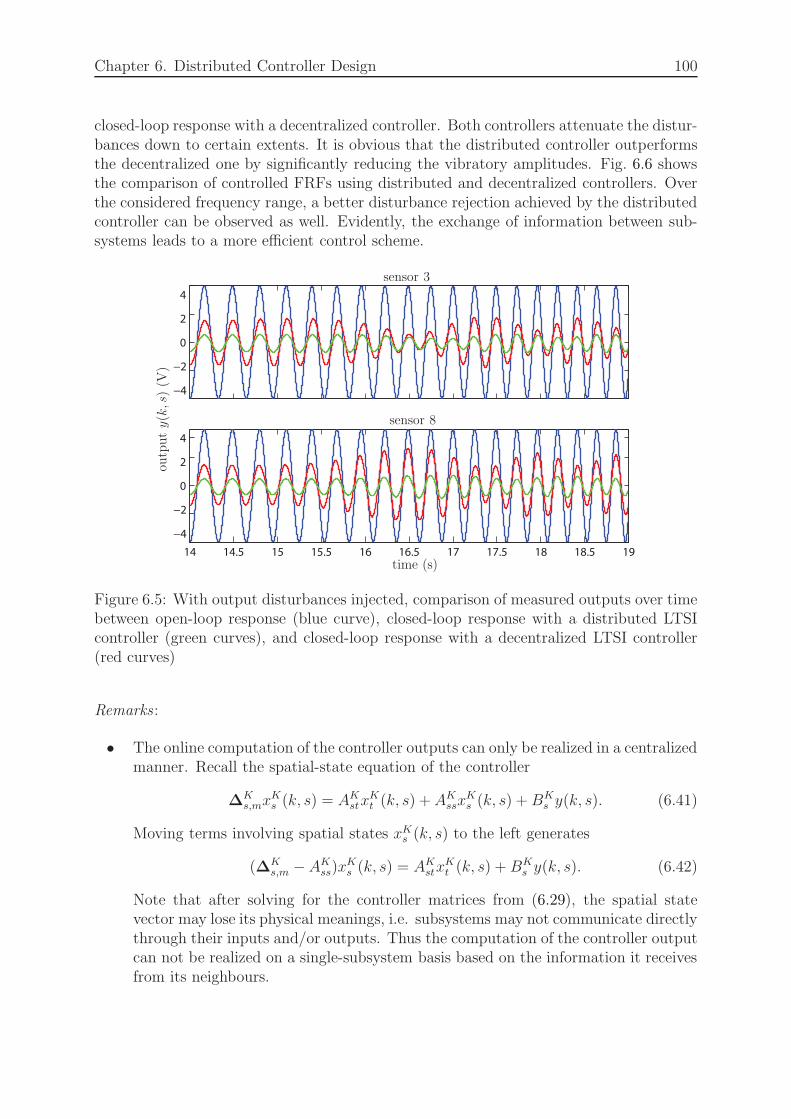
Chapter 6. Distributed Controller Design 100
closed-loop response with a decentralized controller. Both controllers attenuate the distur-bances down to certain extents. It is obvious that the distributed controller outperformsthe decentralized one by significantly reducing the vibratory amplitudes. Fig. 6.6 showsthe comparison of controlled FRFs using distributed and decentralized controllers. Overthe considered frequency range, a better disturbance rejection achieved by the distributedcontroller can be observed as well. Evidently, the exchange of information between sub-systems leads to a more efficient control scheme.
−4
−2
0
2
4
14 14.5 15 15.5 16 16.5 17 17.5 18 18.5 19
−4
−2
0
2
4
time (s)
outputy(k,s)(V
)
sensor 3
sensor 8
Figure 6.5: With output disturbances injected, comparison of measured outputs over timebetween open-loop response (blue curve), closed-loop response with a distributed LTSIcontroller (green curves), and closed-loop response with a decentralized LTSI controller(red curves)
Remarks :
• The online computation of the controller outputs can only be realized in a centralizedmanner. Recall the spatial-state equation of the controller
∆Ks,mx
Ks (k, s) = AK
stxKt (k, s) + AK
ssxKs (k, s) +BK
s y(k, s). (6.41)
Moving terms involving spatial states xKs (k, s) to the left generates
(∆Ks,m −AK
ss)xKs (k, s) = AK
stxKt (k, s) +BK
s y(k, s). (6.42)
Note that after solving for the controller matrices from (6.29), the spatial statevector may lose its physical meanings, i.e. subsystems may not communicate directlythrough their inputs and/or outputs. Thus the computation of the controller outputcan not be realized on a single-subsystem basis based on the information it receivesfrom its neighbours.
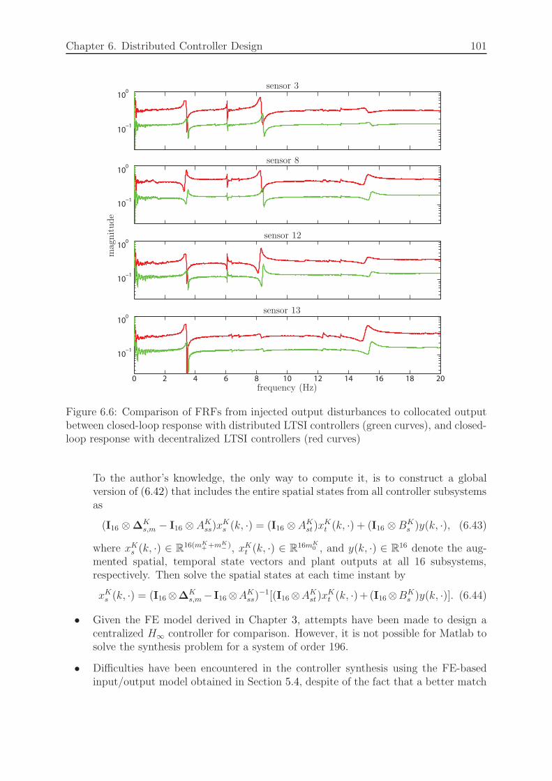
Chapter 6. Distributed Controller Design 101
10−1
100
10−1
100
10−1
100
0 2 4 6 8 10 12 14 16 18 20
10−1
100
frequency (Hz)
magnitude
sensor 3
sensor 8
sensor 12
sensor 13
Figure 6.6: Comparison of FRFs from injected output disturbances to collocated outputbetween closed-loop response with distributed LTSI controllers (green curves), and closed-loop response with decentralized LTSI controllers (red curves)
To the author’s knowledge, the only way to compute it, is to construct a globalversion of (6.42) that includes the entire spatial states from all controller subsystemsas
(I16 ⊗∆Ks,m − I16 ⊗AK
ss)xKs (k, ·) = (I16 ⊗AK
st)xKt (k, ·) + (I16 ⊗BK
s )y(k, ·), (6.43)
where xKs (k, ·) ∈ R
16(mK++mK
−), xK
t (k, ·) ∈ R16mK0 , and y(k, ·) ∈ R16 denote the aug-
mented spatial, temporal state vectors and plant outputs at all 16 subsystems,respectively. Then solve the spatial states at each time instant by
xKs (k, ·) = (I16⊗∆K
s,m− I16⊗AKss)
−1[(I16⊗AKst)x
Kt (k, ·)+ (I16⊗BK
s )y(k, ·)]. (6.44)
• Given the FE model derived in Chapter 3, attempts have been made to design acentralized H∞ controller for comparison. However, it is not possible for Matlab tosolve the synthesis problem for a system of order 196.
• Difficulties have been encountered in the controller synthesis using the FE-basedinput/output model obtained in Section 5.4, despite of the fact that a better match
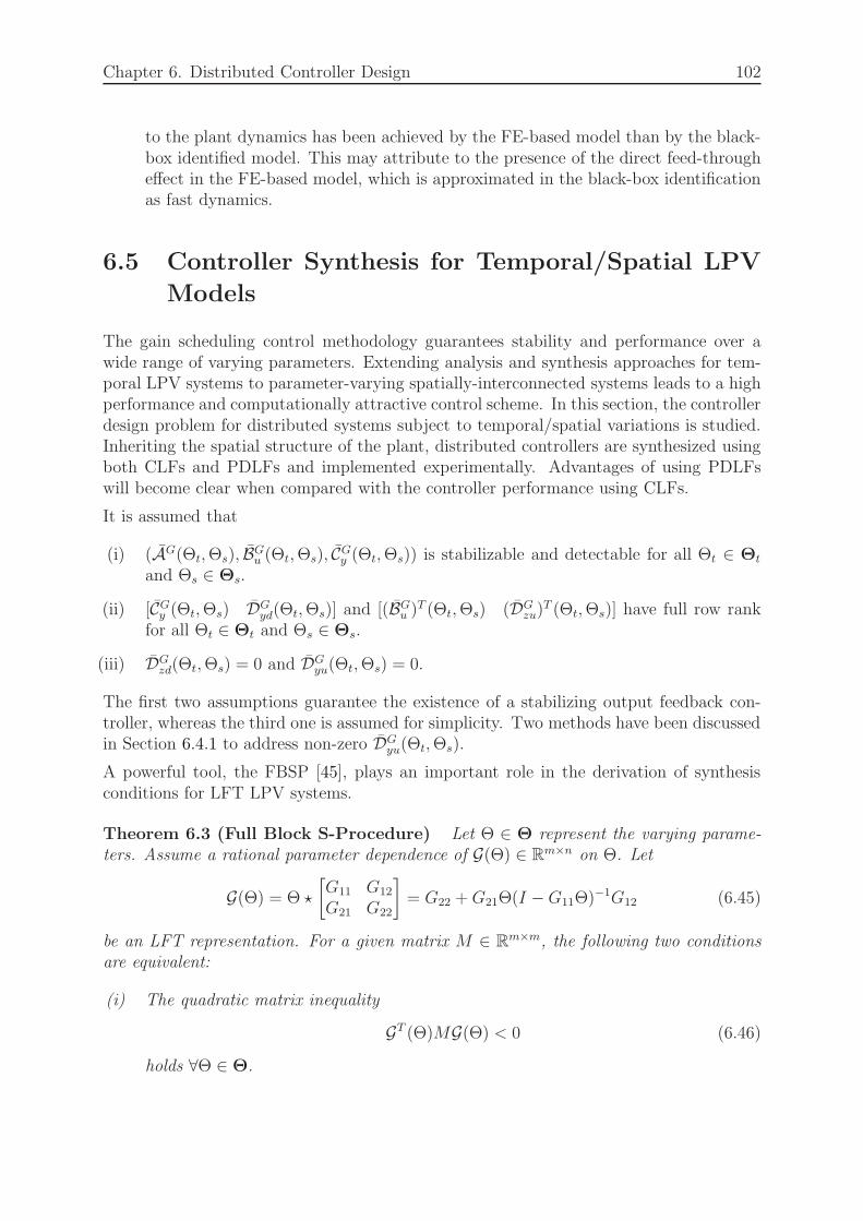
Chapter 6. Distributed Controller Design 102
to the plant dynamics has been achieved by the FE-based model than by the black-box identified model. This may attribute to the presence of the direct feed-througheffect in the FE-based model, which is approximated in the black-box identificationas fast dynamics.
6.5 Controller Synthesis for Temporal/Spatial LPV
Models
The gain scheduling control methodology guarantees stability and performance over awide range of varying parameters. Extending analysis and synthesis approaches for tem-poral LPV systems to parameter-varying spatially-interconnected systems leads to a highperformance and computationally attractive control scheme. In this section, the controllerdesign problem for distributed systems subject to temporal/spatial variations is studied.Inheriting the spatial structure of the plant, distributed controllers are synthesized usingboth CLFs and PDLFs and implemented experimentally. Advantages of using PDLFswill become clear when compared with the controller performance using CLFs.
It is assumed that
(i) (AG(Θt,Θs), BGu (Θt,Θs), CG
y (Θt,Θs)) is stabilizable and detectable for all Θt ∈ Θt
and Θs ∈ Θs.
(ii) [CGy (Θt,Θs) DG
yd(Θt,Θs)] and [(BGu )
T (Θt,Θs) (DGzu)
T (Θt,Θs)] have full row rankfor all Θt ∈ Θt and Θs ∈ Θs.
(iii) DGzd(Θt,Θs) = 0 and DG
yu(Θt,Θs) = 0.
The first two assumptions guarantee the existence of a stabilizing output feedback con-troller, whereas the third one is assumed for simplicity. Two methods have been discussedin Section 6.4.1 to address non-zero DG
yu(Θt,Θs).
A powerful tool, the FBSP [45], plays an important role in the derivation of synthesisconditions for LFT LPV systems.
Theorem 6.3 (Full Block S-Procedure) Let Θ ∈ Θ represent the varying parame-ters. Assume a rational parameter dependence of G(Θ) ∈ Rm×n on Θ. Let
G(Θ) = Θ ⋆
[G11 G12
G21 G22
]
= G22 +G21Θ(I −G11Θ)−1G12 (6.45)
be an LFT representation. For a given matrix M ∈ Rm×m, the following two conditions
are equivalent:
(i) The quadratic matrix inequality
GT (Θ)MG(Θ) < 0 (6.46)
holds ∀Θ ∈ Θ.
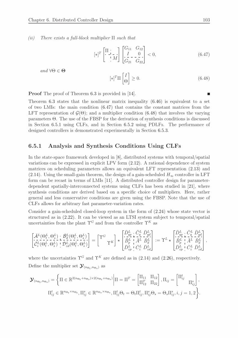
Chapter 6. Distributed Controller Design 103
(ii) There exists a full-block multiplier Π such that
[∗]T[
Π
M
]
G11 G12
I 0
G21 G22
< 0, (6.47)
and ∀Θ ∈ Θ
[∗]TΠ[IΘ
]
≥ 0. (6.48)
Proof The proof of Theorem 6.3 is provided in [14].
Theorem 6.3 states that the nonlinear matrix inequality (6.46) is equivalent to a setof two LMIs: the main condition (6.47) that contains the constant matrices from theLFT representation of G(Θ); and a multiplier condition (6.48) that involves the varyingparameters Θ. The use of the FBSP for the derivation of synthesis conditions is discussedin Section 6.5.1 using CLFs, and in Section 6.5.2 using PDLFs. The performance ofdesigned controllers is demonstrated experimentally in Section 6.5.3.
6.5.1 Analysis and Synthesis Conditions Using CLFs
In the state-space framework developed in [8], distributed systems with temporal/spatialvariations can be expressed in explicit LPV form (2.12). A rational dependence of systemmatrices on scheduling parameters allows an equivalent LFT representation (2.13) and(2.14). Using the small-gain theorem, the design of a gain-scheduled H∞ controller in LFTform can be recast in terms of LMIs [11]. A distributed controller design for parameter-dependent spatially-interconnected systems using CLFs has been studied in [21], wheresynthesis conditions are derived based on a specific choice of multipliers. Here, rathergeneral and less conservative conditions are given using the FBSP. Note that the use ofCLFs allows for arbitrary fast parameter-variation rates.
Consider a gain-scheduled closed-loop system in the form of (2.24) whose state vector isstructured as in (2.22). It can be viewed as an LTSI system subject to temporal/spatialuncertainties from the plant ΥG and from the controller ΥK as
[
AL(ΘLt ,Θ
Ls ) BL
d (ΘLt ,Θ
Ls )
CLz (Θ
Lt ,Θ
Ls ) DL
zd(ΘLt ,Θ
Ls )
]
=
[ΥG
ΥK
]
⋆
DLqp CL
q DLqd
BLp AL BL
d
DLzp CL
z DLzd
:= ΥL ⋆
DLqp CL
q DLqd
BLp AL BL
d
DLzp CL
z DLzd
,
where the uncertainties ΥG and ΥK are defined as in (2.14) and (2.26), respectively.
Define the multiplier set Y (nΘt,nΘs)
as
Y (nΘt,nΘs)
=
Π ∈ R2(nΘt
+nΘs)×2(nΘt+nΘs)
∣∣∣∣Π = ΠT =
[Π11 Π12
ΠT12 Π22
]
,Πij =
[Πt
ij
Πsij
]
,
Πtij ∈ R
nΘt×nΘt ,Πs
ij ∈ RnΘs×nΘs ,Πt
ijΘt = ΘtΠtij,Π
sijΘs = ΘsΠ
sij , i, j = 1, 2
.

Chapter 6. Distributed Controller Design 104
The analysis condition – Theorem 2.2 (ii) – for LTSI systems is extended to distributedLPV systems in the following result.
Theorem 6.4 Assume that the controlled system (2.27) and (2.28) is well-posed. Thesystem is exponentially stable and has quadratic performance γ, for any (ΘL
t ,ΘLs ) ∈
(ΘLt ,Θ
Lt ), if one of following two conditions is satisfied:
(i) There exists a symmetric matrix XL ∈ XmL, such that
[∗∗
]T
0 XL
XL 01γI 0
0 −γI
AL(ΘLt ,Θ
Ls ) BL
d (ΘLt ,Θ
Ls )
I 0
CLz (Θ
Lt ,Θ
Ls ) DL
zd(ΘLt ,Θ
Ls )
0 I
< 0. (6.49)
(ii) There exists a symmetric matrix XL ∈ XmL and a symmetric multiplier ΠL ∈Y (n
ΘLt,n
ΘLs), such that
∗∗∗
T
0 XL
XL 0
ΠL
1γI 0
0 −γI
AL BLp BG
d
I 0 0
CLq DL
qp DLqd
0 I 0
CLz DL
zp DLzd
0 0 I
< 0, (6.50)
and[∗∗
]T
ΠL
[
I
ΥL
]
> 0, (6.51)
where nΘLtand nΘL
sdenote the sizes of temporal and spatial uncertainties of the
closed-loop system, respectively.
Condition (ii) is the result after applying the FBSP to (6.49) with extra constraintsimposed on the multiplier structure, in addition to the symmetry required by the FBSP.
Just like the derivation of synthesis conditions for LTSI systems, the elimination lemmacan not be directly applied to conditions (6.50) and (6.51), due to the unknown partition
of the controller spatial state vector. The restructured state vector xL = [(xG)T (xK)T ]T
requires the permutation of the system matrices, Lyapunov matrices, as well as the mul-tiplier ΠL. The permuted multiplier ΠL has the form
ΠL=
ΠG,t11 ΠGK,t
11
ΠG,s11 ΠGK,s
11
(ΠGK,t11 )T ΠK,t
11
(ΠGK,s11 )T ΠK,s
11
ΠG,t12 ΠGK,t
12
ΠG,s12 ΠGK,s
12
ΠKG,t12 ΠK,t
12
ΠKG,s12 ΠK,s
12
sym
ΠG,t22 ΠGK,t
22
ΠG,s22 ΠGK,s
22
(ΠGK,t22 )T ΠK,t
22
(ΠGK,s22 )T ΠK,s
22
. (6.52)

Chapter 6. Distributed Controller Design 105
Theorem 6.4 (ii) is equivalent to the following results.
Theorem 6.5 The controlled system (2.27) and (2.28) is well-posed, exponentially sta-
ble and has quadratic performance γ if there exists X L in the form of (6.28), and a
multiplier ΠL in the form of (6.52), such that
∗∗∗
T
0 X L
X L 0
ΠL
1γI 0
0 −γI
AL BLp BG
d
I 0 0
C Lq DL
qp DLqd
0 I 0
C Lz DL
zp DLzd
0 0 I
< 0 (6.53)
[∗∗
]T
ΠL
II
ΥG
ΥK
> 0. (6.54)
Controller synthesis conditions can then be further developed by applying the eliminationlemma to (6.53) and (6.54).
Theorem 6.6 Consider a distributed system in LFT form as in (2.16) and (2.17).There exists a distributed controller in the form of (2.25) and (2.26), that guaranteeswell-posedness, exponential stability and quadratic performance γ of the closed-loop sys-tems (2.27) and (2.28), if there exist symmetric matrices R, S ∈ XmG, and symmetricmultipliers ΠR, ΠS ∈ Y (n
ΘGt,n
ΘGs), that satisfy
NTR
∗∗∗
T
0 RR 0
ΠR
1γI 0
0 −γI
(AG)T (CGq )
T (CGz )
T
I 0 0
(BGp )
T (DGqp)
T (DGzp)
T
0 I 0
(BGd )
T (DGqd)
T (DGzd)
T
0 0 I
NR < 0 (6.55)
NTS
∗∗∗
T
0 SS 0
ΠS
1γI 0
0 −γI
AG BGp BG
d
I 0 0
CGq DG
qp DGqd
0 I 0
CGz DG
zp DGzd
0 0 I
NS < 0 (6.56)
[Rt II St
]
≥ 0, (6.57)
and for any Θt ∈ Θt, Θs ∈ Θs
[∗]T
ΠR
[IΥG
]
≥ 0[∗]T
ΠS
[IΥG
]
≥ 0, (6.58)
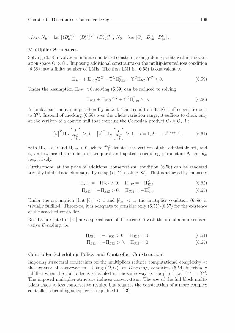
Chapter 6. Distributed Controller Design 106
where NR = ker[(BG
u )T (DG
qu)T (DG
zu)T], NS = ker
[Cy DG
yp DGyd
].
Multiplier Structures
Solving (6.58) involves an infinite number of constraints on gridding points within the vari-ation space Θt×Θs. Imposing additional constraints on the multipliers reduces condition(6.58) into a finite number of LMIs. The first LMI in (6.58) is equivalent to
ΠR11 +ΠR12ΥG +ΥGΠT
R12 +ΥGΠR22ΥG ≥ 0. (6.59)
Under the assumption ΠR22 < 0, solving (6.59) can be reduced to solving
ΠR11 +ΠR12ΥG +ΥGΠT
R12 ≥ 0. (6.60)
A similar constraint is imposed on ΠS as well. Then condition (6.58) is affine with respectto ΥG. Instead of checking (6.58) over the whole variation range, it suffices to check onlyat the vertices of a convex hull that contains the Cartesian product Θt ×Θs, i.e.
[∗]T
ΠR
[I
ΥGi
]
≥ 0,[∗]T
ΠS
[I
ΥGi
]
≥ 0, i = 1, 2, . . . , 22(nt+ns), (6.61)
with ΠR22 < 0 and ΠS22 < 0, where ΥGi denotes the vertices of the admissible set, and
nt and ns are the numbers of temporal and spatial scheduling parameters θt and θs,respectively.
Furthermore, at the price of additional conservatism, condition (6.58) can be renderedtrivially fulfilled and eliminated by using (D,G)-scaling [87]. That is achieved by imposing
ΠR11 = −ΠR22 > 0, ΠR12 = −ΠTR12; (6.62)
ΠS11 = −ΠS22 > 0, ΠS12 = −ΠTS12. (6.63)
Under the assumption that |θti | < 1 and |θsi| < 1, the multiplier condition (6.58) istrivially fulfilled. Therefore, it is adequate to consider only (6.55)-(6.57) for the existenceof the searched controller.
Results presented in [21] are a special case of Theorem 6.6 with the use of a more conser-vative D-scaling, i.e.
ΠR11 = −ΠR22 > 0, ΠR12 = 0; (6.64)
ΠS11 = −ΠS22 > 0, ΠS12 = 0. (6.65)
Controller Scheduling Policy and Controller Construction
Imposing structural constraints on the multipliers reduces computational complexity atthe expense of conservatism. Using (D,G)- or D-scaling, condition (6.54) is triviallyfulfilled when the controller is scheduled in the same way as the plant, i.e. ΥK = ΥG.The imposed multiplier structure induces conservatism. The use of the full block multi-pliers leads to less conservative results, but requires the construction of a more complexcontroller scheduling subspace as explained in [43].
Chapter 6. Distributed Controller Design 107
After Lyapunov matrices R and S, multipliers ΠR and ΠS have been computed, thecontroller can either be constructed using closed-loop formulas, see [21] and [14], orsolved from the analysis conditions (6.53) and (6.54). The closed-loop Lyapunov func-
tion X L is computed in the same way as in the LTSI case (6.33) and (6.34). A gen-eral procedure of constructing the closed-loop multiplier ΠL is provided in [43]. Nev-ertheless, when D-scaling is imposed on the multipliers ΠR and ΠS for simplicity, i.e.ΠR = diagΠR11,−ΠR11 and ΠS = diagΠS11,−ΠS11, the closed-loop multiplier ΠL canbe constructed in the same way as the closed-loop Lyapunov matrix [11], i.e.
PtQTt = I − Πt
R11ΠtS11, PsQ
Ts = I − Πs
R11ΠsS11, (6.66)
then
ΠL,t =
[Πt
S11 I
QTt 0
]−1 [I Πt
R11
0 P Tt
]
, ΠL,s =
[Πs
S11 I
QTs 0
]−1 [I Πs
R11
0 P Ts
]
. (6.67)
The resulting closed-loop multiplier ΠL inherits the structure of D-scaling, i.e.
ΠL =
ΠL,t 00 ΠL,s
−ΠL,t 00 −ΠL,s
. (6.68)
The permuted multiplier ΠL takes the form of (6.52), with ΠL12 = ΠL
21 = 0. The unknownand constant controller matrices in LFT representation in the form of (2.25) can then beeasily solved from (6.53).
6.5.2 Synthesis Conditions Using PDLFs
The use of CLFs to design LPV controllers allows an infinite rate of parameter variationsand results in conservatism, when an upper bound on the variation rate exists. Thesmaller the bounds, the more conservative is the use of CLFs. This section extends thecontroller design approach in [14] for temporal LFT systems to distributed LFT LPVsystems using PDLFs.
Define ∂X (Θt,Θs) as the variation rate of a Lyapunov function X (Θt,Θs) ∈ Xm. Assumethat the varying dynamics of the temporal and spatial variables are decoupled, then
∂X (Θt,Θs) =
[∂tXt(Θt)
∂sXs(Θs)
]
, (6.69)
where ∂t and ∂s denote the derivatives with respect to time and space, respectively. Letthe set of temporal and spatial variation rates of uncertainties be denoted by (Ξt,Ξs),such that (Θt,Θs) ∈ (Θt,Θs), and (∂tΘt, ∂sΘs) ∈ (Ξt,Ξs).
After incorporating the parameter-dependent Lyapunov functions, the system analysisconditions are formulated as follows.

Chapter 6. Distributed Controller Design 108
Theorem 6.7 Assume that the controlled system (2.27) and (2.28) is well-posed. Thesystem is exponentially stable and has quadratic performance γ, if one of following twoconditions is satisfied:
(i) There exists a Lyapunov matrix X L(ΘLt ,Θ
Ls ) in the form of (6.28) with respect to per-
muted closed-loop uncertainties (ΘLt ,Θ
Ls ), such that for any (ΘL
t ,ΘLs ) ∈ (ΘL
t ,ΘLs ),
(∂tΘLt , ∂sΘ
Ls ) ∈ (ΞL
t ,ΞLs )
[∗∗
]T
0 X L(ΘLt ,Θ
Ls )
X L(ΘLt ,Θ
Ls ) −∂X L(ΘL
t ,ΘLs )
1γI 0
0 −γI
AL(ΘLt ,Θ
Ls ) BL
d (ΘLt ,Θ
Ls )
I 0
CLz (Θ
Lt ,Θ
Ls ) DL
zd(ΘLt ,Θ
Ls )
0 I
< 0,
(6.70)
where (ΘLt ,Θ
Ls ) are the sets of permuted closed-loop uncertainties.
(ii) There exist Lyapunov matrices R(Θt,Θs), S(Θt,Θs) ∈ XmG, such that for any(Θt,Θs) ∈ (Θt,Θs), (∂tΘt, ∂sΘs) ∈ (Ξt,Ξs)
[∗]T[∗∗
]T
0 R(Θt,Θs)R(Θt,Θs) −∂R(Θt,Θs)
1γI 0
0 −γI
(AG)T (Θt,Θs) (CGz )
T (Θt,Θs)I 0
(BGd )
T (Θt,Θs) (DGzd)
T (Θt,Θs)0 I
×NR(Θt,Θs) < 0, (6.71)
[∗]T[∗∗
]T
0 S(Θt,Θs)S(Θt,Θs) ∂S(Θt,Θs)
1γI 0
0 −γI
AG(Θt,Θs) BGd (Θt,Θs)
I 0
CGz (Θt,Θs) DG
zd(Θt,Θs)0 I
×NS(Θt,Θs) < 0, (6.72)
[Rt(Θt) I
I St(Θt)
]
≥ 0, (6.73)
where
NR(Θt,Θs) = ker[(BG
u )T (Θt,Θs) (DG
zu)T (Θt,Θs)
], (6.74)
NS(Θt,Θs) = ker[CGy (Θt,Θs) DG
yd(Θt,Θs)]. (6.75)
Condition (ii) is the result of applying the elimination lemma to (6.70).
To solve the infinite set of LMIs (6.71)-(6.73), two commonly used approaches are
1. gridding [18], where inequalities are solved at grid points that cover the range ofparameter variation and rates (Θt,Θs)× (Ξt,Ξs);
Chapter 6. Distributed Controller Design 109
2. LFT LPV synthesis, which relies on the application of S-procedure [88], or theextended version - FBSP.
Considered here is LFT LPV controller synthesis. Assume a quadratic form of the Lya-punov matrices R(Θt,Θs) and S(Θt,Θs), and bring the parameter-varying system ma-trices and null spaces in their LFT representations, respectively. After performing themultiplications of LFT systems, conditions (6.71)-(6.73) can be rewritten as
[∗]T
0 PP 0
1γI 0
0 −γI
(
Ω ⋆
[GP11 GP12
GP21 GP22
])
< 0 (6.76)
[∗]T
0 QQ 0
1γI 0
0 −γI
(
Ω ⋆
[GQ11 GQ12
GQ21 GQ22
])
< 0 (6.77)
[∗]T
Pt 00 Qt
0 II 0
([Θt
Θt
]
⋆
[G11 G12
G21 G22
])
≥ 0, (6.78)
where P , Q ∈ XmG ; the augmented plant uncertainty Ω arises from the LFT multi-plication in (6.71) and (6.72), and is defined as Ω = diag∂ΥG,ΥG,ΥG,ΥG,ΥG. Thederivation from (6.71)-(6.73) to (6.76)-(6.78), and the algebraic expressions of the con-stant matrices in (6.76)-(6.78) can be found in Appendix B. It is easy to see that thequadratic matrix inequalities (6.76)-(6.78) are now in the form of (6.46). Applying theFBSP to each of them results in the following synthesis conditions.
Theorem 6.8 Consider an LTSV system (2.16) and (2.17) with its parameter variationand rate sets (Θt,Θs) and (Ξt,Ξs), respectively. There exists a distributed LPV controllerin the form of (2.23), that guarantees well-posedness, exponential stability and quadraticperformance γ of the closed-loop system (2.24), if there exist matrices P , Q ∈ XmG,multipliers ΠP , ΠQ ∈ Y (5n
ΘGt,5n
ΘGs) and Π ∈ Y (2n
ΘGt,2n
ΘGt), that satisfy
[∗∗
]T
ΠP
0 PP 0
1γI 0
0 −γI
GP11 GP12
I 0
GP21 GP22
< 0, (6.79)
[∗∗
]T
ΠQ
0 QQ 0
1γI 0
0 −γI
GQ11 GQ12
I 0
GQ21 GQ22
< 0, (6.80)

Chapter 6. Distributed Controller Design 110
[∗∗
]T
−Π
Pt 00 Qt
0 II 0
G11 G12
I 0
G21 G22
≥ 0, (6.81)
and ∀(Θt,Θs) ∈ (Θt,Θs), (∂tΘt, ∂sΘs) ∈ (Ξt,Ξs)
[∗]TΠP
[IΩ
]
≥ 0, (6.82)
[∗]TΠQ
[IΩ
]
≥ 0, (6.83)
[∗∗
]T
Π
II
Θt
Θt
> 0. (6.84)
Proof The proof of Theorem 6.8 can be found in Appendix B.
Controller Construction
Discussions on the multiplier structures in Section 6.5.1 for the controller design usingCLFs apply when PDLFs are used. If the quadratic LFT matrix functions R(Θt,Θs) andS(Θt,Θs) have been found after solving (6.79)–(6.84), to the author’s knowledge, the LPVcontroller can only be constructed using explicit formulas, see [14] and [18]. Nevertheless,due to the use of gain-scheduled Lyapunov functions, the implementation of the designedcontroller in the form of (2.23) requires the real-time measurement of the parametervariation rates. Under the assumption of decoupled temporal and spatial variations, thederivatives of spatial parameters can be measured off-line and remain unchanged on-line.However, it is often difficult to estimate the temporal variation rate. Thus, in order toremove the controller dependence on ∂tΘt, only one of the Lyapunov matrices R(Θt,Θs)or S(Θt,Θs) is defined as parameter-varying [13], e.g. let R be constant and S(Θt,Θs)be parameter-dependent. For the sake of brevity, the argument (Θt,Θs) of a parameter-dependent matrix is left out in the following equations, e.g. a calligraphic A is short forA(Θt,Θs), whereas R stands for a constant matrix. The continuous LPV controller isobtained as
N = I − SR,
F =− [(DGzu)
T DGzu]
−1 × [γ(BGu )
TR−1 + (DGzu)
T CGz ],
L =− [γS−1(CGy )
T + Bd(DGyd)
T ]× [DGyd(DG
yd)T ]−1,
AK =−N−1((AG)T + S[AG + BG
u F + LCGy ]R + γ−1S[BG
d + LDGyd](BG
d )T
+ γ−1(CGz )
T [CGz + DG
zuF ]R),
BK = N−1SL,CK = FR,
DK = 0.
Chapter 6. Distributed Controller Design 111
6.5.3 Experimental Results
The experimental setup is modified as a spatially-varying system by deactivating sixactuator/sensor pairs just as for the LPV model identification in Chapter 5. The controlobjective is defined in the same way as in the LTSI case in Section 6.4.3—suppressingparallel injected output disturbances. Based on the black-box identified spatial LPVmodel, distributed controllers using both CLFs and PDLFs have been designed by shapingmixed sensitivities, and have been validated experimentally.
• Distributed controller using CLFs: Multipliers with D-scalings are used. The re-sulting controller is of temporal order mK
0 = 5, and of spatial order mK+ = mK
− = 4.
• Distributed controller using PDLFs: Multipliers with D-scalings are used. Due tothe spatial variation of the subsystem, the parameter-dependent Lyapunov matrixis a function of spatial uncertainties. A quadratic Lyapunov matrix can be writtenin LFT form as
R(Θs) =
[Rt
Rs(Θs)
]
= T TR (Θs)PTR(Θs) = [∗]T
[
Pt
Ps
] [I
TRs(Θs)
]
= [∗]T[
Pt
Ps
]
I
Θs ⋆
[TRs11 TRs12
TRs21 TRs22
]
=[∗]T[
Pt
Ps
]
Θs ⋆
TRs11 0 TRs12
0 I 0TRs21 0 TRs22
.
(6.85)
Let Rs(Θs) be a first order polynomial in Θs, i.e. Rs(Θs) = P0+P1Θs, which yieldsthe following selection
Ps =
[0 P1/2
P1/2 P0
]
,
[TRs11 TRs12
TRs21 TRs22
]
=
0 I
I 00 I
. (6.86)
The obtained controller is of temporal order mK0 = 4, and of spatial order mK
+ =mK
− = 4.
Fig. 6.7 shows the comparison of the experimental responses in time domain betweenopen loop and closed-loop system with controllers designed using both PDLFs and CLFs.Fig. 6.8 shows the comparison in frequency domain—FRFs from injected output distur-bance to collocated output. The distributed controller designed using PDLFs improvesthe closed-loop performance significantly at most of the subsystems, especially in the lowfrequency range. Provided the knowledge of the upper bound on the spatial variationrate, the conservatism caused by the use of CLFs is largely reduced by the use of PDLFs.The improved experimental results confirm the benefits of using PDLFs.
6.6 Summary
This chapter has addressed the distributed controller design problem for both LTSI andLTSV systems, where a controller inheriting the distributed nature of the plant is desired.
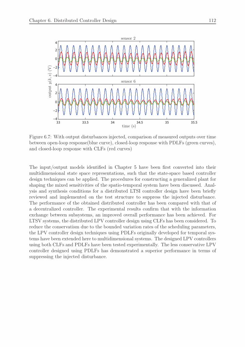
Chapter 6. Distributed Controller Design 112
−4
−2
0
2
4
33 33.5 34 34.5 35 35.5
−4
−2
0
2
4
time (s)
outputy(k,s)(V
)
sensor 2
sensor 6
Figure 6.7: With output disturbances injected, comparison of measured outputs over timebetween open-loop response(blue curve), closed-loop response with PDLFs (green curves),and closed-loop response with CLFs (red curves)
The input/output models identified in Chapter 5 have been first converted into theirmultidimensional state space representations, such that the state-space based controllerdesign techniques can be applied. The procedures for constructing a generalized plant forshaping the mixed sensitivities of the spatio-temporal system have been discussed. Anal-ysis and synthesis conditions for a distributed LTSI controller design have been brieflyreviewed and implemented on the test structure to suppress the injected disturbance.The performance of the obtained distributed controller has been compared with that ofa decentralized controller. The experimental results confirm that with the informationexchange between subsystems, an improved overall performance has been achieved. ForLTSV systems, the distributed LPV controller design using CLFs has been considered. Toreduce the conservatism due to the bounded variation rates of the scheduling parameters,the LPV controller design techniques using PDLFs originally developed for temporal sys-tems have been extended here to multidimensional systems. The designed LPV controllersusing both CLFs and PDLFs have been tested experimentally. The less conservative LPVcontroller designed using PDLFs has demonstrated a superior performance in terms ofsuppressing the injected disturbance.
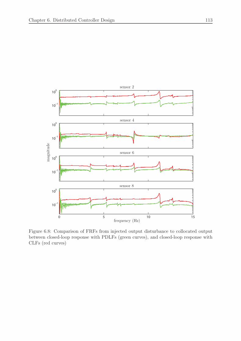
Chapter 6. Distributed Controller Design 113
10−1
100
10−1
100
10−1
100
0 5 10 15
10−1
100
frequency (Hz)
magnitude
sensor 2
sensor 4
sensor 6
sensor 8
Figure 6.8: Comparison of FRFs from injected output disturbance to collocated outputbetween closed-loop response with PDLFs (green curves), and closed-loop response withCLFs (red curves)

Chapter 7
Distributed Anti-WindupCompensator Design
7.1 Introduction
Actuator saturation often occurs in physical systems. The constrained control behaviour isusually not captured when solving the controller design problem as described in Chapter 6.In the presence of limitations on the actuator capacity, the established closed-loop perfor-mance suffers from deterioration, or even instability. For this reason, anti-windup (AW)compensators are often considered in real applications to counteract the effects of actuatorsaturation.
Over the last decades, AW compensator design has been addressed in numerous works byapplying various approaches. A linear conditioning scheme that augments a system witha linear transfer function as the AW compensator, which results from the right coprimefactorisation of the plant, is proposed in [36], aiming at driving the saturated system backto the intended linear behaviour as quickly as possible. In [39], provided that stabilityis guaranteed for a constrained system, performance can be tuned by minimizing the L2
gain using a static compensator. This approach is further developed in [37] [89] witha compensator of order greater than or equal to that of the plant. AW compensatorsthat handle the controller saturation as well as plant uncertainties are considered in[38]. In [42], a more general and potentially less conservative framework for the robustanalysis of nonlinearities is developed, which is applied to solve the AW compensatordesign problem in [90] and [91]. The common feature of the aforementioned works isa two-step approach, where the synthesis problems are solved separately, one after theother, for the controller and the AW compensator. Different from the conventional two-step approach, [92] computes the controller and the AW compensator in one step with onegoal, where the gridding method is employed to solve the resulting nonlinear inequalities.
Among the existing works, very few deal with the saturation problem of distributed pa-rameter systems. In [40], a robust AW compensator for the reaction-diffusion equation ispresented. The centralized scheme may encounter difficulties when applied to a large scalesystem. Instead of a large model describing the system dynamics in a centralized manner,
114

Chapter 7. Distributed Anti-Windup Compensator Design 115
a localized model of smaller size is much easier to handle. Working in the distributedsystem framework developed in [8], [41] proposes a distributed AW compensator for anopen-water channel control system, which boils down to the search for a static gain valuethat guarantees Lyapunov stability.
Inspired by the work in [41], [89] and [37], this chapter proposes an AW compensatordesign using a two-step approach for LTSI systems. The designed AW compensator canbe implemented on top of an existing closed-loop system, with global stability and abound on L2 performance of the augmented system guaranteed. The tool developed in[42] – the IQC approach – is employed to impose constraints on the nonlinear saturationoperator, such that the analysis and synthesis conditions can be formulated in terms ofLMIs.
This chapter includes results reported in [93]. The rest of this chapter is organized asfollows: Section 7.2 recaps a lumped AW architecture, and the framework of IQCs, withan emphasis on its application to the saturation/deadzone operator, and robust analysis.Section 7.3 extends the AW scheme for lumped systems to spatially-interconnected sys-tems. In Section 7.3.1, stability analysis via IQCs is applied to constrained distributedsystems. Synthesis conditions for an AW compensator are derived in Section 7.3.2. Adecentralized AW scheme is designed for comparison in Section 7.4. Simulation resultsobtained on an actuated Euler-Bernoulli beam demonstrate the performance of both thedistributed and the decentralized AW schemes in Section 7.5.
7.2 Preliminary
This section recaps the working principle of a lumped AW scheme with full-order dynam-ics. A mathematical tool – IQCs – that is often used to analyse the robust stability of afeedback system with nonlinear uncertainties is reviewed here, and will be employed laterfor the derivation of system analysis conditions.
7.2.1 AW Scheme for Lumped Systems
The two-step AW design, also referred to as control of constrained systems [94], consistsof two steps:
1. Design a linear controller K, such that when |u| ≤ u, where u is the maximumcapacity of the physical actuators, stability and a performance bound are guaranteedon the closed-loop system.
2. Design a linear AW compensator Ψ, such that when |u| > u, the achieved stabilityand performance from step 1 are preserved to a certain extent.
The AW framework for lumped systems proposed in [89] is shown in Fig. 7.1. Whenactuator saturation does not occur, u = u0 holds; otherwise, the AW compensator Ψ isactivated and generates two compensation signals: v1 ∈ R
nu is added to the controller

Chapter 7. Distributed Anti-Windup Compensator Design 116
output, while v2 ∈ Rny enters the controller as part of the controlled input, i.e., y = y0+v2.The state space realization of the AW compensator suggested in [89]
xΨ(k + 1)[v1(k)v2(k)
]
=
[
AΨ BΨ
CΨ DΨ
][
xΨ(k)
e(k)
]
, (7.1)
where e = u− u, possesses full-order dynamics, and allows more degrees of freedom thana static compensator. The saturation operator is defined as
u = sat(u0 + v1) = sat(u), (7.2)
where sat(u) = sign(u) ∗minu, |u|.
GK
Ψ
y u0 u u
d
z
y0
ev2
v1
Figure 7.1: AW scheme proposed for lumped systems in [89]
7.2.2 Robust Analysis Using IQCs
IQCs [42] can be used to analyse systems with various types of uncertainties. It describesthe behaviour of a system in the frequency domain in terms of an integral constraint onthe Fourier transformations of the input/output signals [95].
Let RH∞ be the set of proper, stable and rational functions with real coefficients, Ll2(0,∞)
be the space of square integrable signals, i.e., a signal f(t) ∈ Ll2(0,∞), if its energy
‖ f(t) ‖2=∫ ∞
0
‖ f(τ) ‖2 dτ (7.3)
is bounded. The definition of IQCs is given as follows.
Definition 7.1 (IQC [42]) Two signals w ∈ Lm2 (0,∞) and v ∈ Ll
2(0,∞) are said tosatisfy the IQC defined by a Hermitian-valued function Π, where Π : jR → C(l+m)×(l+m),if
∫ ∞
−∞
[v(jw)w(jw)
]∗
Π(jw)
[v(jw)w(jw)
]
dw ≥ 0, (7.4)
where v(jw) and w(jw) are the Fourier transformations of v and w, respectively.

Chapter 7. Distributed Anti-Windup Compensator Design 117
Provided a proper choice of the multiplier Π, IQCs can be used to describe relations be-
tween signals. For example, with the multiplier Π =
[I 00 −I
]
, (7.4) defines ‖ w ‖2≤‖ v ‖2.
Multiplier for Saturation/Deadzone Operator
With the definition of the saturation operator given, the deadzone operator is defined ase = dz(u) = u − sat(u); both of them are nonlinear operators. By allowing additionalconservatism, the saturation and deadzone operators can be over-bounded by a linearoperator – sector [0 1] – as shown in Fig. 7.2.
e
uu
u
uu
−u−u
(a) (b)
Figure 7.2: Sector [0 1] bounds a saturation operator (a) and a deadzone operator (b)
Consider now only the deadzone function. The fact that the deadzone operator is boundedby a sector [0 1] implies that for any positive definite symmetric matrix W ∈ Rnu×nu , thecondition
eT W (u− e) ≥ 0 (7.5)
holds, which can be reformulated as a quadratic matrix inequality as
2eT W u− 2eT W e ≥ 0, (7.6)
eT W u+ uTW e− 2eT W e ≥ 0, (7.7)
[∗]T[−2W W
W 0
] [eu
]
≥ 0. (7.8)
Therefore a static multiplier Π :=
[−2W W
W 0
]
can be used to cast the nonlinear deadzone
function into a quadratic constraint.
Stability Analysis
The characterization of a nonlinear operator in terms of (7.4) makes sense only whenthe involved signals are bounded, such that their square integral exists. Thus, stabilityanalysis on the feedback loop as shown in Fig. 7.3 is required.
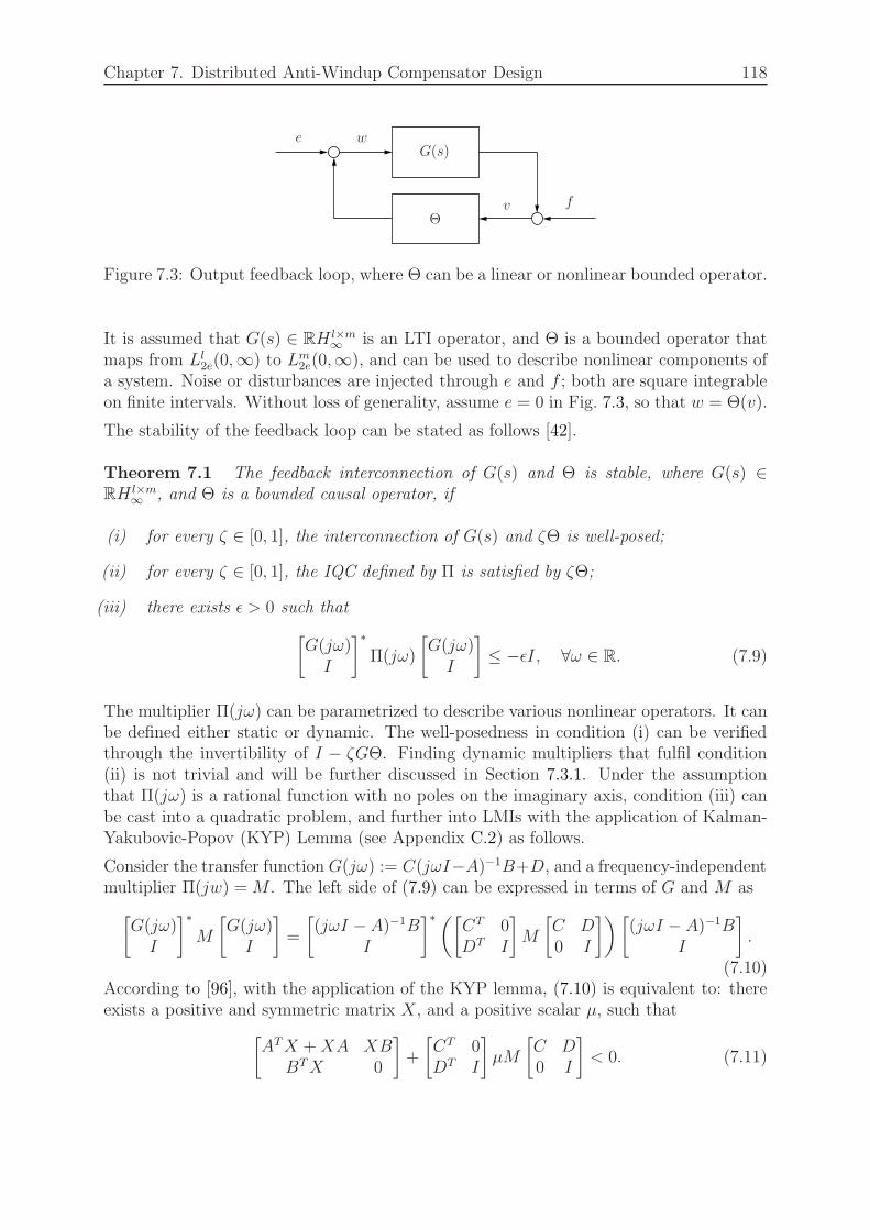
Chapter 7. Distributed Anti-Windup Compensator Design 118
G(s)
Θ
e w
v f
Figure 7.3: Output feedback loop, where Θ can be a linear or nonlinear bounded operator.
It is assumed that G(s) ∈ RH l×m∞ is an LTI operator, and Θ is a bounded operator that
maps from Ll2e(0,∞) to Lm
2e(0,∞), and can be used to describe nonlinear components ofa system. Noise or disturbances are injected through e and f ; both are square integrableon finite intervals. Without loss of generality, assume e = 0 in Fig. 7.3, so that w = Θ(v).
The stability of the feedback loop can be stated as follows [42].
Theorem 7.1 The feedback interconnection of G(s) and Θ is stable, where G(s) ∈RH l×m
∞ , and Θ is a bounded causal operator, if
(i) for every ζ ∈ [0, 1], the interconnection of G(s) and ζΘ is well-posed;
(ii) for every ζ ∈ [0, 1], the IQC defined by Π is satisfied by ζΘ;
(iii) there exists ǫ > 0 such that
[G(jω)
I
]∗
Π(jω)
[G(jω)
I
]
≤ −ǫI, ∀ω ∈ R. (7.9)
The multiplier Π(jω) can be parametrized to describe various nonlinear operators. It canbe defined either static or dynamic. The well-posedness in condition (i) can be verifiedthrough the invertibility of I − ζGΘ. Finding dynamic multipliers that fulfil condition(ii) is not trivial and will be further discussed in Section 7.3.1. Under the assumptionthat Π(jω) is a rational function with no poles on the imaginary axis, condition (iii) canbe cast into a quadratic problem, and further into LMIs with the application of Kalman-Yakubovic-Popov (KYP) Lemma (see Appendix C.2) as follows.
Consider the transfer function G(jω) := C(jωI−A)−1B+D, and a frequency-independentmultiplier Π(jw) = M . The left side of (7.9) can be expressed in terms of G and M as
[G(jω)
I
]∗
M
[G(jω)
I
]
=
[(jωI −A)−1B
I
]∗([CT 0DT I
]
M
[C D0 I
])[(jωI − A)−1B
I
]
.
(7.10)According to [96], with the application of the KYP lemma, (7.10) is equivalent to: thereexists a positive and symmetric matrix X , and a positive scalar µ, such that
[ATX +XA XB
BTX 0
]
+
[CT 0DT I
]
µM
[C D0 I
]
< 0. (7.11)
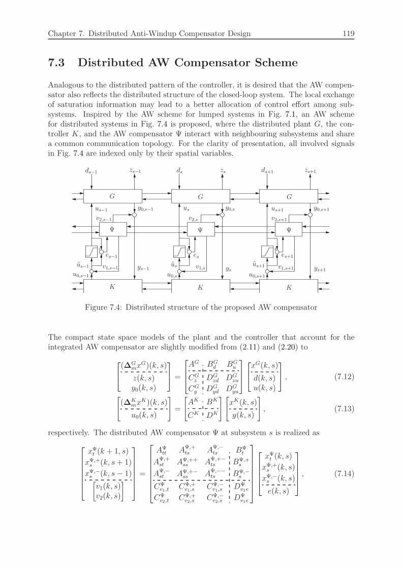
Chapter 7. Distributed Anti-Windup Compensator Design 119
7.3 Distributed AW Compensator Scheme
Analogous to the distributed pattern of the controller, it is desired that the AW compen-sator also reflects the distributed structure of the closed-loop system. The local exchangeof saturation information may lead to a better allocation of control effort among sub-systems. Inspired by the AW scheme for lumped systems in Fig. 7.1, an AW schemefor distributed systems in Fig. 7.4 is proposed, where the distributed plant G, the con-troller K, and the AW compensator Ψ interact with neighbouring subsystems and sharea common communication topology. For the clarity of presentation, all involved signalsin Fig. 7.4 are indexed only by their spatial variables.
GGG
KKK
ΨΨΨ
ds−1 zs−1 ds zs ds+1 zs+1
us−1 y0,s−1
v2,s−1
es−1
us−1 v1,s−1
u0,s−1
ys−1
us y0,s
v2,s
esus v1,s
u0,s
ys
us+1 y0,s+1
v2,s+1
es+1
us+1 v1,s+1
u0,s+1
ys+1
Figure 7.4: Distributed structure of the proposed AW compensator
The compact state space models of the plant and the controller that account for theintegrated AW compensator are slightly modified from (2.11) and (2.20) to
(∆Gmx
G)(k, s)
z(k, s)y0(k, s)
=
AG BGd BG
u
CGz DG
zd DGzu
CGy DG
yd DGyu
xG(k, s)
d(k, s)u(k, s)
, (7.12)
[
(∆Kmx
K)(k, s)
u0(k, s)
]
=
[
AK BK
CK DK
][
xK(k, s)
y(k, s)
]
, (7.13)
respectively. The distributed AW compensator Ψ at subsystem s is realized as
xΨt (k + 1, s)
xΨ,+s (k, s+ 1)
xΨ,−s (k, s− 1)[v1(k, s)v2(k, s)
]
=
AΨtt AΨ,+
ts AΨ,−ts BΨ
t
AΨ,+st AΨ,++
ss AΨ,+−ts BΨ,+
s
AΨ,−st AΨ,+−
ss AΨ,−−ts BΨ,−
s
CΨv1,t
CΨ,+v1,s
CΨ,−v1,s
DΨv1e
CΨv2,t
CΨ,+v2,s
CΨ,−v2,s
DΨv1e
xΨt (k, s)
xΨ,+s (k, s)
xΨ,−s (k, s)
e(k, s)
, (7.14)
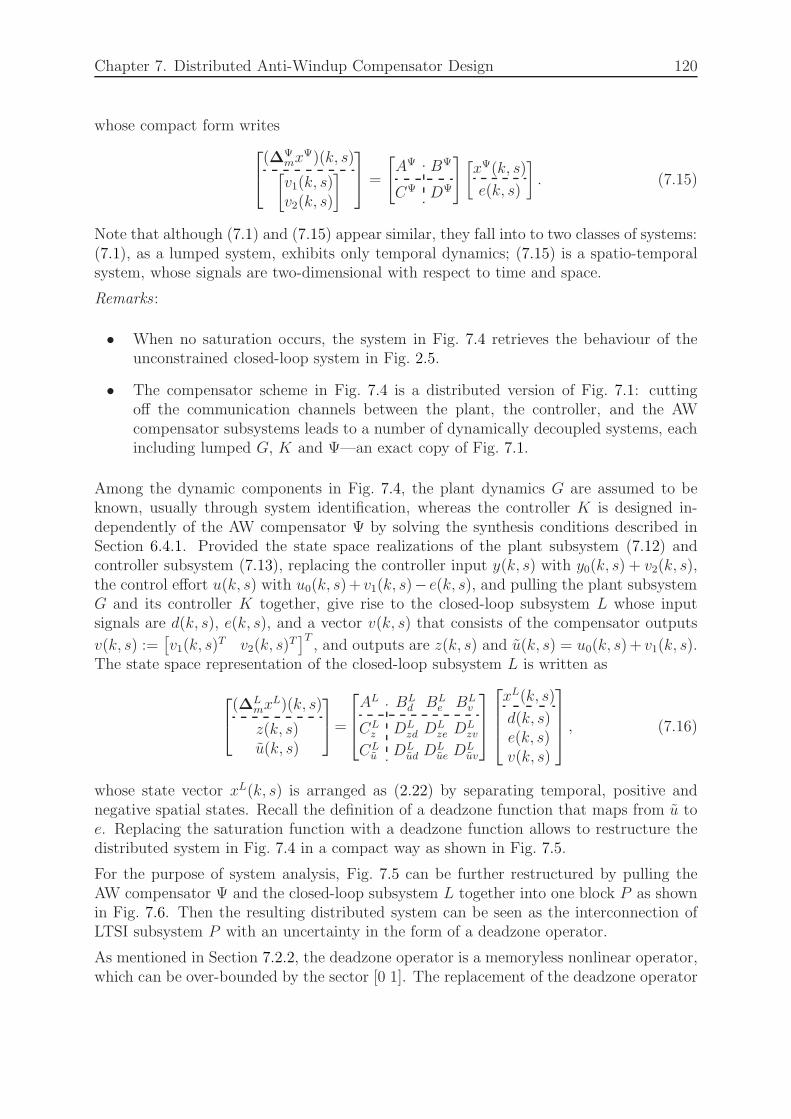
Chapter 7. Distributed Anti-Windup Compensator Design 120
whose compact form writes
(∆Ψmx
Ψ)(k, s)[v1(k, s)v2(k, s)
]
=
[
AΨ BΨ
CΨ DΨ
][xΨ(k, s)
e(k, s)
]
. (7.15)
Note that although (7.1) and (7.15) appear similar, they fall into to two classes of systems:(7.1), as a lumped system, exhibits only temporal dynamics; (7.15) is a spatio-temporalsystem, whose signals are two-dimensional with respect to time and space.
Remarks :
• When no saturation occurs, the system in Fig. 7.4 retrieves the behaviour of theunconstrained closed-loop system in Fig. 2.5.
• The compensator scheme in Fig. 7.4 is a distributed version of Fig. 7.1: cuttingoff the communication channels between the plant, the controller, and the AWcompensator subsystems leads to a number of dynamically decoupled systems, eachincluding lumped G, K and Ψ—an exact copy of Fig. 7.1.
Among the dynamic components in Fig. 7.4, the plant dynamics G are assumed to beknown, usually through system identification, whereas the controller K is designed in-dependently of the AW compensator Ψ by solving the synthesis conditions described inSection 6.4.1. Provided the state space realizations of the plant subsystem (7.12) andcontroller subsystem (7.13), replacing the controller input y(k, s) with y0(k, s) + v2(k, s),the control effort u(k, s) with u0(k, s)+ v1(k, s)− e(k, s), and pulling the plant subsystemG and its controller K together, give rise to the closed-loop subsystem L whose inputsignals are d(k, s), e(k, s), and a vector v(k, s) that consists of the compensator outputs
v(k, s) :=[v1(k, s)
T v2(k, s)T]T, and outputs are z(k, s) and u(k, s) = u0(k, s)+ v1(k, s).
The state space representation of the closed-loop subsystem L is written as
(∆Lmx
L)(k, s)
z(k, s)u(k, s)
=
AL BLd BL
e BLv
CLz DL
zd DLze D
Lzv
CLu DL
ud DLue D
Luv
xL(k, s)
d(k, s)e(k, s)v(k, s)
, (7.16)
whose state vector xL(k, s) is arranged as (2.22) by separating temporal, positive andnegative spatial states. Recall the definition of a deadzone function that maps from u toe. Replacing the saturation function with a deadzone function allows to restructure thedistributed system in Fig. 7.4 in a compact way as shown in Fig. 7.5.
For the purpose of system analysis, Fig. 7.5 can be further restructured by pulling theAW compensator Ψ and the closed-loop subsystem L together into one block P as shownin Fig. 7.6. Then the resulting distributed system can be seen as the interconnection ofLTSI subsystem P with an uncertainty in the form of a deadzone operator.
As mentioned in Section 7.2.2, the deadzone operator is a memoryless nonlinear operator,which can be over-bounded by the sector [0 1]. The replacement of the deadzone operator
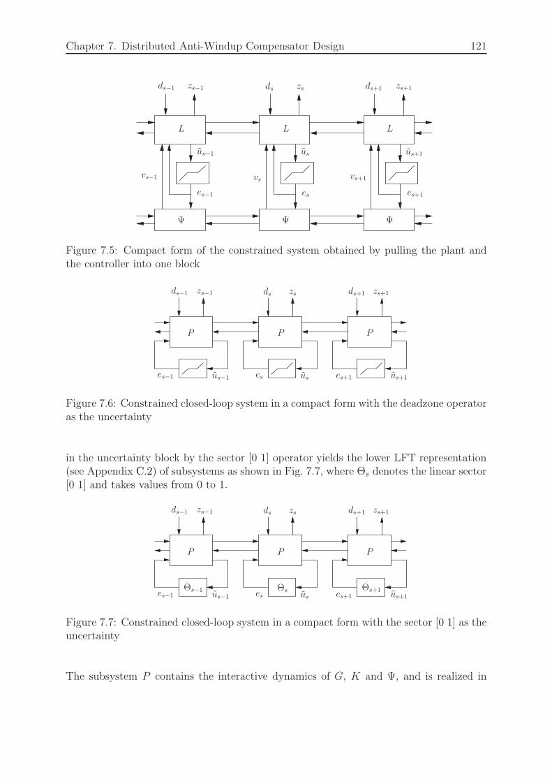
Chapter 7. Distributed Anti-Windup Compensator Design 121
LLL
Ψ Ψ Ψ
ds−1 zs−1 ds zs ds+1 zs+1
us−1
vs−1
es−1
us
vs
es
us+1
vs+1
es+1
Figure 7.5: Compact form of the constrained system obtained by pulling the plant andthe controller into one block
PPP
ds−1 zs−1 ds zs ds+1 zs+1
es−1 us−1 es us es+1 us+1
Figure 7.6: Constrained closed-loop system in a compact form with the deadzone operatoras the uncertainty
in the uncertainty block by the sector [0 1] operator yields the lower LFT representation(see Appendix C.2) of subsystems as shown in Fig. 7.7, where Θs denotes the linear sector[0 1] and takes values from 0 to 1.
PPP
ds−1 zs−1 ds zs ds+1 zs+1
es−1 us−1 es us es+1 us+1
Θs−1 Θs Θs+1
Figure 7.7: Constrained closed-loop system in a compact form with the sector [0 1] as theuncertainty
The subsystem P contains the interactive dynamics of G, K and Ψ, and is realized in

Chapter 7. Distributed Anti-Windup Compensator Design 122
LFT form as
(∆Pmx
P )(k, s)
z(k, s)u(k, s)
=
AP BPd BP
e
CPz DP
zd DPze
CPu DP
ud DPue
xP (k, s)
d(k, s)e(k, s)
(7.17)
e(k, s) = Θsu(k, s), (7.18)
whose state vector is grouped as
xP =
[[xLt
xΨt
]T
,
[xLs+
xΨs+
]T
,
[xLs−
xΨs−
]T]T
. (7.19)
With the matrices of subsystem L known, after grouping the unknown AW parameterstogether, the system matrices of subsystem P can be decomposed as
ALtt 0 AL,+
ts 0 AL,−ts 0 BL
t,d BLt,e
0 0 0 0 0 0 0 0
AL,+st 0 AL,++
ss 0 AL,+−ss 0 BL,+
s,d BL,+s,e
0 0 0 0 0 0 0 0
AL,−st 0 AL,−+
ss 0 AL,−−ss 0 BL,−
s,d BL,−s,e
0 0 0 0 0 0 0 0
CLt,z 0 CL,+
s,z 0 CL,−s,z 0 DL
zd DLze
CLt,u 0 CL,+
s,u 0 CL,−s,u 0 DL
ud DLue
+
0 0 0 BLt,v
I 0 0 00 0 0 BL,+
s,v
0 I 0 00 0 0 BL,−
s,v
0 0 I 0
0 0 0 DLzv
0 0 0 DLuv
[
AΨ BΨ
CΨ DΨ
]
0 I 0 0 0 0 0 00 0 0 I 0 0 0 00 0 0 0 0 I 0 00 0 0 0 0 0 0 I
.
(7.20)
7.3.1 Analysis Conditions
Theorem 7.1 states conditions for a lumped feedback loop in Fig. 7.3 to be stable. Replacethe LTI operator G(s) in Fig. 7.3 with the LTSI subsystem P in Fig. 7.6, the uncertaintyblock Θ with Θs. The stability theorem 7.1 can be extended to spatially distributedsystems as follows.
Theorem 7.2 Assume that the distributed plant G in (7.12), the distributed controllerK in (7.13) and the distributed AW compensator Ψ in (7.15) are given. The intercon-nected system (7.17) and (7.18) is well-posed, exponentially stable and satisfies quadraticperformance γ, if there exists a symmetric positive definite matrix W ∈ Rnu×nu and a realmatrix XP ∈ XmP , such that
∗∗∗
T
0 XP
XP 0
−γI 00 1
γI
−2W WW 0
I 0 0AP BP
d BPe
0 I 0CP
z DPzd DP
ze
0 0 ICP
u DPud DP
ue
< 0 (7.21)
holds.

Chapter 7. Distributed Anti-Windup Compensator Design 123
Proof Consider now the state space realization (7.17) of subsystem P . Impose a worst-case gain γ on the performance channel d → z. After applying the KYP lemma C.2 (seeAppendix C), condition (iii) in Theorem 7.1 is equivalent to the existence of a Lyapunovmatrix XP ∈ XmP , and a positive scalar µ ([42] [97]), such that
(AP )TXP +XP AP XP BPd XP BP
e
(BPd )
TXP 0 0
(BPe )
TXP 0 −I
+1
γ2
(CPz )
T
(DPzd)
T
(DPze)
T
[CP
z DPzd DP
ze
]
+
(CPu )
T 0
(DPud)
T 0
(DPue)
T I
µM
[CP
u DPud DP
ue
0 0 I
]
< 0, (7.22)
where the static multiplier that characterizes the sector [0 1] operator is selected as
M =
[0 W
W −2W
]
. (7.23)
Provided that the upper left term in the chosen multiplier is positive semi-definite, con-dition (ii) in Theorem 7.1 is always fulfilled for ζ = 0. Meanwhile, the negative semi-definiteness of the lower right terms turns (7.4) into a convex problem. Therefore, itsuffices to check condition (ii) only at ζ = 1 [42], which is trivially fulfilled. Thus, stabil-ity of the well-posed interconnected system between subsystem P and a deadzone operatorΨ has been established.
Finally, with the change of variable W = µW , (7.22) can be written in a quadraticinequality form as (7.21).
Remarks :
• According to the sector condition, (7.5) should hold for any positive symmetricmatrices W (or W ). Defining W as a variable in (7.21) allows extra degrees offreedom in the minimization of γ.
• Despite the conservatism of a sector-based boundary [98], sector [0 1] is widelyapplied in control engineering to impose constraints on a deadzone/saturation op-erator. The conservatism could be reduced with the use of dynamic (frequency-dependent) multipliers [99] [100].
7.3.2 Synthesis Conditions
With the analysis conditions developed in Theorem 7.2, synthesis conditions for a dis-tributed AW compensator Ψ can be easily obtained by applying the elimination lemmanot to (7.21) directly, but to the permuted version of (7.21), due to the same argumentas made during the derivation of the controller synthesis conditions in Chapter 6, i.e.,the sizes of positive and negative spatial states of the compensator remain unknown until

Chapter 7. Distributed Anti-Windup Compensator Design 124
the synthesis is complete. Instead of a closed-loop realization as in (7.20), a restructured
state space model with the state vector defined as xP (k, s) =
[xL(k, s)xΨ(k, s)
]
is given by
AP BPd BP
e
C Pz DP
zd DPze
C Pu DP
ud DPue
=
AL 0 BLd BL
e
0 0 0 0
CLz 0 DL
zd DLze
CLu 0 DL
ud DLue
+
0 BLv
I 0
0 DLzv
0 DLuv
[
AΨ BΨ
CΨ DΨ
] [0 I 0 00 0 0 I
]
︸ ︷︷ ︸
Q
. (7.24)
The Lyapunov matrix XP ∈ XmP is accordingly permuted in the same way as in (6.28),i.e.
X P =
XLt XLΨ
t
XLs XLΨ
s
(XLΨt )T XΨ
t
(XLΨs )T XΨ
s
. (7.25)
Theorem 7.2 is equivalent to: The interconnected system (7.17) and (7.18) is well-posed,exponentially stable and satisfies quadratic performance γ, if there exists a symmetricpositive definite matrix W ∈ Rnu×nu and a real matrix X P in the form of (7.25), suchthat
∗∗∗
T
0 X P
X P 0
−γI 00 1
γI
−2W WW 0
I 0 0
AP BPd BP
e
0 I 0
CPz DP
zd DPze
0 0 I
CPu DP
ud DPue
< 0. (7.26)
Inheriting the distributed fashion of the controller design, a local AW compensator is tobe designed based on a single subsystem, and copied to all other subsystems in case of anLTSI system. Conditions for the design of a distributed AW compensator can be derivedas follows.
Theorem 7.3 There exists a distributed AW compensator Ψ in (7.15), that guaranteeswell-posedness, exponential stability and quadratic performance γ of the constrained closed-loop system (7.17) and (7.18), if there exist a symmetric positive definite matrix W ∈Rnu×nu and R, S ∈ XmL, that satisfy
[∗∗
]T
0 SS 0
−γI 00 1
γI
I 0AL BL
d
0 ICL
z DLzd
< 0, (7.27)
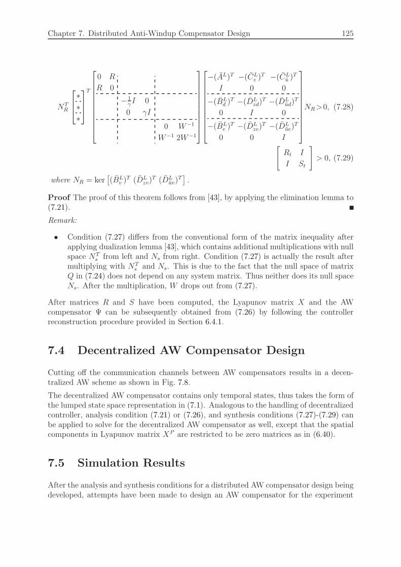
Chapter 7. Distributed Anti-Windup Compensator Design 125
NTR
∗∗∗
T
0 R
R 0
− 1γI 0
0 γI
0 W−1
W−1 2W−1
−(AL)T −(CLz )
T −(CLu )
T
I 0 0
−(BLd )
T −(DLzd)
T −(DLud)
T
0 I 0
−(BLe )
T −(DLze)
T −(DLue)
T
0 0 I
NR>0, (7.28)
[
Rt I
I St
]
> 0, (7.29)
where NR = ker[(BL
v )T (DL
zv)T (DL
uv)T].
Proof The proof of this theorem follows from [43], by applying the elimination lemma to(7.21).
Remark:
• Condition (7.27) differs from the conventional form of the matrix inequality afterapplying dualization lemma [43], which contains additional multiplications with nullspace NT
s from left and Ns from right. Condition (7.27) is actually the result aftermultiplying with NT
s and Ns. This is due to the fact that the null space of matrixQ in (7.24) does not depend on any system matrix. Thus neither does its null spaceNs. After the multiplication, W drops out from (7.27).
After matrices R and S have been computed, the Lyapunov matrix X and the AWcompensator Ψ can be subsequently obtained from (7.26) by following the controllerreconstruction procedure provided in Section 6.4.1.
7.4 Decentralized AW Compensator Design
Cutting off the communication channels between AW compensators results in a decen-tralized AW scheme as shown in Fig. 7.8.
The decentralized AW compensator contains only temporal states, thus takes the form ofthe lumped state space representation in (7.1). Analogous to the handling of decentralizedcontroller, analysis condition (7.21) or (7.26), and synthesis conditions (7.27)-(7.29) canbe applied to solve for the decentralized AW compensator as well, except that the spatialcomponents in Lyapunov matrix XP are restricted to be zero matrices as in (6.40).
7.5 Simulation Results
After the analysis and synthesis conditions for a distributed AW compensator design beingdeveloped, attempts have been made to design an AW compensator for the experiment
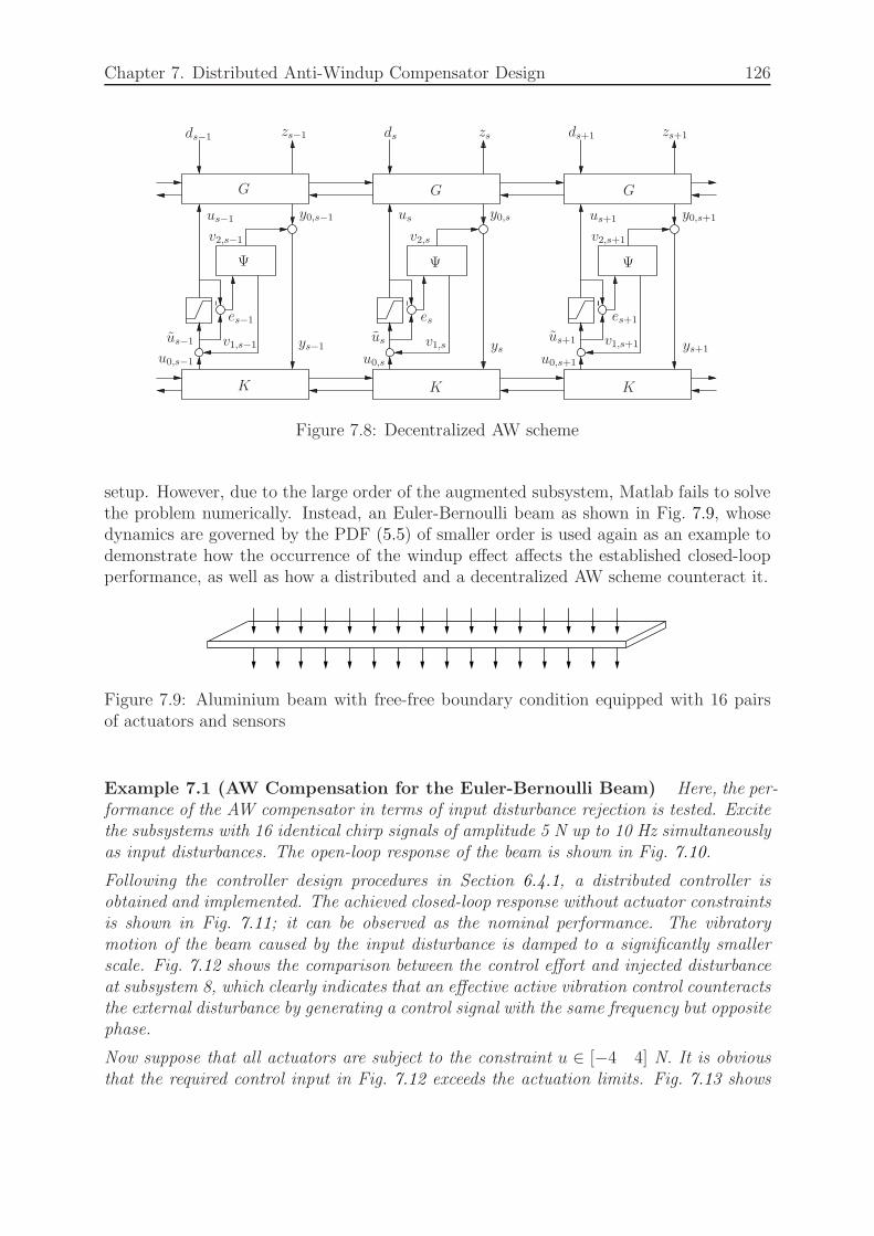
Chapter 7. Distributed Anti-Windup Compensator Design 126
GGG
KKK
ΨΨΨ
ds−1 zs−1 ds zs ds+1 zs+1
us−1 y0,s−1
v2,s−1
es−1
us−1 v1,s−1
u0,s−1
ys−1
us y0,s
v2,s
esus v1,s
u0,s
ys
us+1 y0,s+1
v2,s+1
es+1
us+1 v1,s+1
u0,s+1
ys+1
Figure 7.8: Decentralized AW scheme
setup. However, due to the large order of the augmented subsystem, Matlab fails to solvethe problem numerically. Instead, an Euler-Bernoulli beam as shown in Fig. 7.9, whosedynamics are governed by the PDF (5.5) of smaller order is used again as an example todemonstrate how the occurrence of the windup effect affects the established closed-loopperformance, as well as how a distributed and a decentralized AW scheme counteract it.
Figure 7.9: Aluminium beam with free-free boundary condition equipped with 16 pairsof actuators and sensors
Example 7.1 (AW Compensation for the Euler-Bernoulli Beam) Here, the per-formance of the AW compensator in terms of input disturbance rejection is tested. Excitethe subsystems with 16 identical chirp signals of amplitude 5 N up to 10 Hz simultaneouslyas input disturbances. The open-loop response of the beam is shown in Fig. 7.10.
Following the controller design procedures in Section 6.4.1, a distributed controller isobtained and implemented. The achieved closed-loop response without actuator constraintsis shown in Fig. 7.11; it can be observed as the nominal performance. The vibratorymotion of the beam caused by the input disturbance is damped to a significantly smallerscale. Fig. 7.12 shows the comparison between the control effort and injected disturbanceat subsystem 8, which clearly indicates that an effective active vibration control counteractsthe external disturbance by generating a control signal with the same frequency but oppositephase.
Now suppose that all actuators are subject to the constraint u ∈ [−4 4] N. It is obviousthat the required control input in Fig. 7.12 exceeds the actuation limits. Fig. 7.13 shows

Chapter 7. Distributed Anti-Windup Compensator Design 127
00.2
0.40.6
0.81
0
1
2
3
4
5
0
0.2
0.4
0.6
time (s)beam coordinate (m)
displacement(m
)
Figure 7.10: Open-loop response to 16 parallel chirp signals up to 10 Hz as input distur-bances
00.2
0.40.6
0.81
0
1
2
3
4
5
−0.0002
−0.0001
0
0.0001
0.0002
time (s)beam coordinate (m)
displacement(m
)
Figure 7.11: Closed-loop response to 16 parallel chirp signals up to 10 Hz as input dis-turbances without actuator constraints
the closed-loop performance achieved by the same controller with actuator constraints.Although worse than Fig. 7.11, it is still better than the open-loop response. The windupeffect can be observed in Fig. 7.14, where in (a) the controller output u0(k, 8) is windedup to a considerably high level, whereas (b) shows the control signal after saturation.
Fig. 7.15 shows the closed-loop response with the distributed AW scheme, and Fig. 7.17with the decentralized AW scheme. The distributed AW compensator improves the perfor-mance, compared to Fig. 7.13, but not to the level of the nominal closed-loop performancein Fig. 7.11—in principle, any AW scheme can hardly recover the unconstrained per-

Chapter 7. Distributed Anti-Windup Compensator Design 128
0 0.1 0.2 0.3 0.4 0.5 0.6 0.7 0.8 0.9 1−6
−4
−2
0
2
4
6
time (s)
u0(k,8)vs.
d(k,8)(N
)
Figure 7.12: Control effort (blue curve) and input disturbance (red curve) at subsystem8, without actuator constraints. The required control effort exceeds the max. and min.actuation limits (green lines).
00.2
0.40.6
0.81
0
1
2
3
4
5
−0.2
−0.1
0
0.1
time (s)beam coordinate (m)
displacement(m
)
Figure 7.13: Closed-loop response to 16 parallel chirp signals up to 10 Hz as input dis-turbances with actuator constraints imposed, without AW implemented
formance. Fig. 7.16 shows how the attenuation of saturated control effort is realized bythe distributed AW scheme. The counteracting of distributed AW output v1 against theexcessive controller output u0, effectively brings the saturated system behaviour back toits linear range. With the information exchanging between subsystems, the control effortcan be better allocated to counteract the saturation effects. The decentralized compensatorin Fig. 7.17 clearly destabilizes the system. However, it should be noted that this is notthe general case. For a fair comparison in this work, the same shaping filters have beenemployed to tune the decentralized and distributed AW compensator design. It turns outthat the decentralized AW compensator destabilizes the constrained system.

Chapter 7. Distributed Anti-Windup Compensator Design 129
0
0
0
4
-4
2
-2
-2000
2000
4000
10.1 0.2 0.3 0.4 0.5 0.6 0.7 0.8 0.9
time (s)
u0(k,8)(N
)u(k,8)(N
)
(a)
(b)
Figure 7.14: Controller output u0(k, s) in (a) and saturated control effort u(k, s) in (b) atsubsystem 8 with actuator constraints imposed
00.2
0.40.6
0.81
0
1
2
3
4
5
−0.005
0
0.005
0.01
0.015
time (s)beam coordinate (m)
displacement(m
)
Figure 7.15: Closed-loop response to 16 parallel chirp signals up to 10 Hz as input dis-turbances with actuator constraints imposed, with a distributed AW compensator imple-mented
7.6 Summary
This chapter has proposed a two-step approach for the distributed AW compensatordesign to counteract the actuator saturation that often occurs in physical systems. A
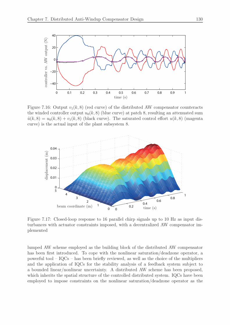
Chapter 7. Distributed Anti-Windup Compensator Design 130
0 0.1 0.2 0.3 0.4 0.5 0.6 0.7 0.8 0.9 1
−40
−20
0
20
40
time (s)
controllervs.
AW
output(N
)
Figure 7.16: Output v1(k, 8) (red curve) of the distributed AW compensator counteractsthe winded controller output u0(k, 8) (blue curve) at patch 8, resulting an attenuated sumu(k, 8) = u0(k, 8) + v1(k, 8) (black curve). The saturated control effort u(k, 8) (magentacurve) is the actual input of the plant subsystem 8.
00.2
0.40.6
0.81
0
1
2
3
4
5
0
0.01
0.02
0.03
0.04
time (s)beam coordinate (m)
displacement(m
)
Figure 7.17: Closed-loop response to 16 parallel chirp signals up to 10 Hz as input dis-turbances with actuator constraints imposed, with a decentralized AW compensator im-plemented
lumped AW scheme employed as the building block of the distributed AW compensatorhas been first introduced. To cope with the nonlinear saturation/deadzone operator, apowerful tool – IQCs – has been briefly reviewed, as well as the choice of the multipliersand the application of IQCs for the stability analysis of a feedback system subject toa bounded linear/nonlinear uncertainty. A distributed AW scheme has been proposed,which inherits the spatial structure of the controlled distributed system. IQCs have beenemployed to impose constraints on the nonlinear saturation/deadzone operator as the

Chapter 7. Distributed Anti-Windup Compensator Design 131
uncertainty, such that the compensator design problem can be cast in terms of LMIs. Theproposed distributed AW scheme has been compared with a decentralized AW scheme;both designed compensators have been tested in simulation to address the saturationproblem of a beam structure governed by the Euler-Bernoulli equation. The simulationresults demonstrated that by enforcing the communication between subsystems in thedistributed AW scheme, the control effort can be more efficiently allocated to counteractthe saturation effects than in the decentralized one.
Chapter 8
Conclusions and Outlook
This thesis has studied physical modelling, identification, controller and AW compensatordesign of spatially-distributed systems. An aluminium beam equipped with an array ofcollocated piezo actuator/sensor pairs has been constructed as a representative spatially-distributed system for experimental use. The aim is to realize an effective model-basedcontroller design to achieve given performance specifications on the closed-loop system.The state space framework developed in [8] provides the foundation of the thesis. Newmethods have been developed to address problems arising during implementation.
A physical model has been constructed in Chapter 3 using a piezoelectric FE modellingapproach, which incorporates an array of piezo actuators and sensors into the modelling.The obtained theoretical FE model has been updated by performing the experimentalmodal analysis. A good match between the updated FE model and measured structuraldynamics has been achieved. Possible reasons for unmodeled effects have been analysed.A direct feed-through phenomenon has been observed between collocated actuators andsensors.
Physical modelling by means of exploring the underlying physical laws may become diffi-cult if the plant dynamics get complex. Chapter 4 has proposed an approach to identifythe FRF matrix directly from the input/output behaviour of the plant. Provided FRFmeasurements at a small number of selected actuating and sensing locations, a local LPVidentification technique for spatio-temporal systems has been proposed to parametrizethe FRF matrix as a spatial LPV model, allowing to approximate FRFs at unmeasuredactuation or sensing locations. The proposed method thus alleviates tedious experimentalwork in case of a complex structure. Experimental results demonstrate the feasibility ofthis approach.
Considering a spatially-distributed system as the interconnection of an array of subsys-tems, Chapter 5 addressed the identification problem in a distributed framework. Thetwo-dimensional least-squares based estimation methods developed in [27] for LTSI mod-els and in [29] for LTSV models have been experimentally implemented. To improvethe identification accuracy especially at resonances, a new identification procedure hasbeen developed by making use of the FE modelling results obtained in Chapter 3. The
132
Chapter 8. Conclusions and Outlook 133
identified models provide a better representation of the real structural dynamics than theblack-box models.
Analysis and synthesis conditions for spatially-invariant systems proposed in [8] have beenimplemented experimentally in Chapter 6 for the first time to suppress the structural vi-bration of an actuated beam. The closed-loop performance of the distributed controllerhas been compared to that of a decentralized controller. The information exchange withina distributed controller allows each subsystem to obtain information about the status ofits neighbours; it helps to achieve an improved overall performance. The LPV controllerdesign technique using PDLFs has been extended from lumped systems to LTSV sys-tems. Spatial LPV controllers have been designed for the test structure which consists ofspatially-varying subsystems using both CLFs and PDLFs. The experimental comparisonconfirms that, with the reduced conservatism, an LPV controller designed using PDLFsoutperforms the corresponding one using CLFs.
Chapter 7 has dealt with the actuator saturation problem that often occurs in a physicalsystem. A distributed AW scheme has been proposed, that preserves the distributednature of the plant and the designed controller. IQCs have been applied to analysethe robust stability of the saturated system. A distributed AW compensator has beensynthesized using the Euler-Bernoulli beam as an example. Its performance has beencompared in simulation with that of a decentralized AW scheme. Due to the more efficientallocation of control effort among subsystems, the distributed AW scheme recovers theclosed-loop performance better than the decentralized one in the presence of actuatorsaturation.
Outlook
Aspects that should be taken into consideration in future research are summarized asfollows:
• The experimental identification of distributed systems often requires a large spatialorder to achieve an accurate approximation of the test structure. Experience showsthat, after the implementation of the controller synthesis procedure, the obtainedcontroller has normally the same order as the generalized plant. Furthermore, if adistributed AW scheme is built on top of them to counteract actuator saturation,the AW compensator has a size of both the plant and the controller. The largesystem order imposes numerical challenges on the search for optimal solutions whensolving synthesis LMIs: either the LMIs can not be handled by the LMI solvers;or the results are sensitive to numerical errors. Therefore, keeping the model orderas small as possible can be essential for LMI solvers to find a feasible and reliablesolution. Taking the coupled temporal and spatial dynamics into consideration,structure-preserving model reduction [101] is one interesting option to simplify amultidimensional model.
• In this work, the construction of a generalized plant for controller synthesis is basedon the use of one-dimensional shaping filters by only shaping the temporal dynam-ics of the closed-loop system. Although it has demonstrated its performance to acertain extent in terms of disturbance rejection, the power of robust controller de-
Chapter 8. Conclusions and Outlook 134
sign through shaping sensitivities has not been fully explored in multidimensionalsystems. It has been mentioned that the use of two-dimensional shaping filters maypotentially lead to an improved performance, where the filter itself is a distributedsystem. To find the appropriate parametrization of a two-dimensional shaping filterwhich imposes desired constraints on the closed-loop system is not a trivial task. Itleaves room for further research on the impact of the use of two-dimensional shapingfilters.
• Before applying the well-developed state-space based synthesis conditions in [8], theexperimentally identified input/output model needs to be realized in state spacerepresentation. Alternatively, analysis and synthesis conditions could be directlyderived and implemented in input/output form. Two main advantages of employinginput/output synthesis are:
– It has been discussed in Section 6.4.3 that after solving for the controller ma-trices, the online computation of the controller outputs can only be realizedin a centralized manner as depicted in Fig. 1.6. In contrast, a distributedcontroller in input/output form allows to implement the online computationin a ’real’ distributed architecture as shown in Fig. 1.2 (c), where subsystemscommunicate with each other through inputs and/or outputs.
– It has been mentioned in Section 6.2.2 that the equivalence between the spatialLPV input/output model and its state space representation is not influencedby the dynamic dependence on the scheduling parameters in this specific ap-plication. Nevertheless, when it is not this case, the complexity in terms ofrealizing an equivalent state space model can increase significantly. This moti-vates the development of synthesis techniques that can design temporal/spatialLPV controllers directly from the identified input/output LPV models. Rel-evant methods have been developed for lumped systems, e.g. [102], [82], etc.A distributed fixed-structure controller design approach for LTSI systems isproposed in [103].
• This thesis works on the modelling, identification and controller design of an exper-imental setup, with an array of piezo actuators and sensors attached in a collocatedpattern. It has been studied in [51], that the use of collocated actuator/sensor pairsfor a lightly damped flexible structure leads to alternating poles and zeros near theimaginary axis. This property guarantees the asymptotic stability of the controlledsystem against disturbances and uncertainties; thus it is recommended. It has beenobserved in Chapter 3, that a direct feed-through effect exists between collocatedactuators and sensors. Although the sensor measurements could be compensatedusing a feed-through constant, the presence of the direct feed-through effect causedseveral difficulties in identification and controller design.
– It has been demonstrated that the feed-through constants slightly vary frompatch to patch. The use of an identical feed-through constant for all subsystemsbrings inaccuracy into the modelling and identification. On the other hand,the use of varying feed-through constants violates the LTSI assumption.
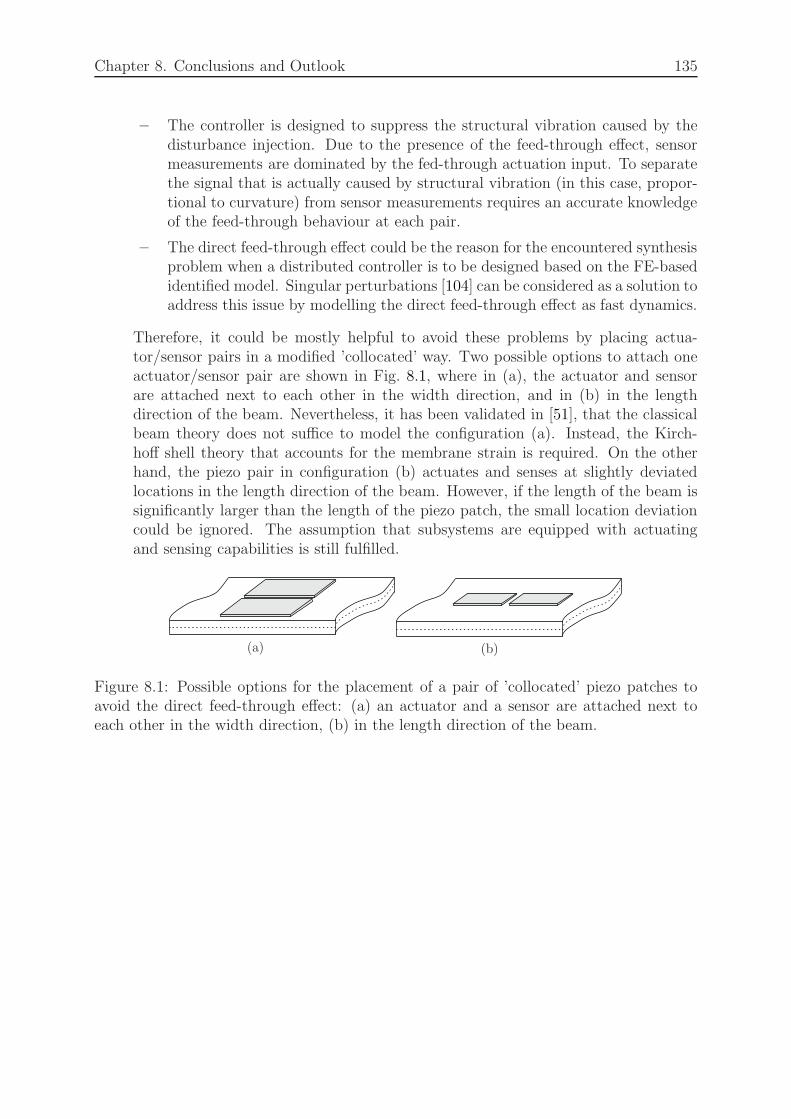
Chapter 8. Conclusions and Outlook 135
– The controller is designed to suppress the structural vibration caused by thedisturbance injection. Due to the presence of the feed-through effect, sensormeasurements are dominated by the fed-through actuation input. To separatethe signal that is actually caused by structural vibration (in this case, propor-tional to curvature) from sensor measurements requires an accurate knowledgeof the feed-through behaviour at each pair.
– The direct feed-through effect could be the reason for the encountered synthesisproblem when a distributed controller is to be designed based on the FE-basedidentified model. Singular perturbations [104] can be considered as a solution toaddress this issue by modelling the direct feed-through effect as fast dynamics.
Therefore, it could be mostly helpful to avoid these problems by placing actua-tor/sensor pairs in a modified ’collocated’ way. Two possible options to attach oneactuator/sensor pair are shown in Fig. 8.1, where in (a), the actuator and sensorare attached next to each other in the width direction, and in (b) in the lengthdirection of the beam. Nevertheless, it has been validated in [51], that the classicalbeam theory does not suffice to model the configuration (a). Instead, the Kirch-hoff shell theory that accounts for the membrane strain is required. On the otherhand, the piezo pair in configuration (b) actuates and senses at slightly deviatedlocations in the length direction of the beam. However, if the length of the beam issignificantly larger than the length of the piezo patch, the small location deviationcould be ignored. The assumption that subsystems are equipped with actuatingand sensing capabilities is still fulfilled.
(a) (b)
Figure 8.1: Possible options for the placement of a pair of ’collocated’ piezo patches toavoid the direct feed-through effect: (a) an actuator and a sensor are attached next toeach other in the width direction, (b) in the length direction of the beam.
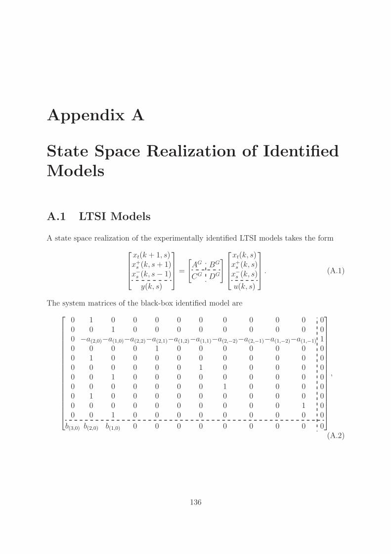
Appendix A
State Space Realization of IdentifiedModels
A.1 LTSI Models
A state space realization of the experimentally identified LTSI models takes the form
xt(k + 1, s)x+s (k, s+ 1)
x−s (k, s− 1)
y(k, s)
=
[
AG BG
CG DG
]
xt(k, s)x+s (k, s)
x−s (k, s)
u(k, s)
. (A.1)
The system matrices of the black-box identified model are
0 1 0 0 0 0 0 0 0 0 0 00 0 1 0 0 0 0 0 0 0 0 00 −a(2,0)−a(1,0)−a(2,2)−a(2,1)−a(1,2)−a(1,1)−a(2,−2)−a(2,−1)−a(1,−2)−a(1,−1) 10 0 0 0 1 0 0 0 0 0 0 00 1 0 0 0 0 0 0 0 0 0 00 0 0 0 0 0 1 0 0 0 0 00 0 1 0 0 0 0 0 0 0 0 00 0 0 0 0 0 0 1 0 0 0 00 1 0 0 0 0 0 0 0 0 0 00 0 0 0 0 0 0 0 0 0 1 00 0 1 0 0 0 0 0 0 0 0 0
b(3,0) b(2,0) b(1,0) 0 0 0 0 0 0 0 0 0
,
(A.2)
136
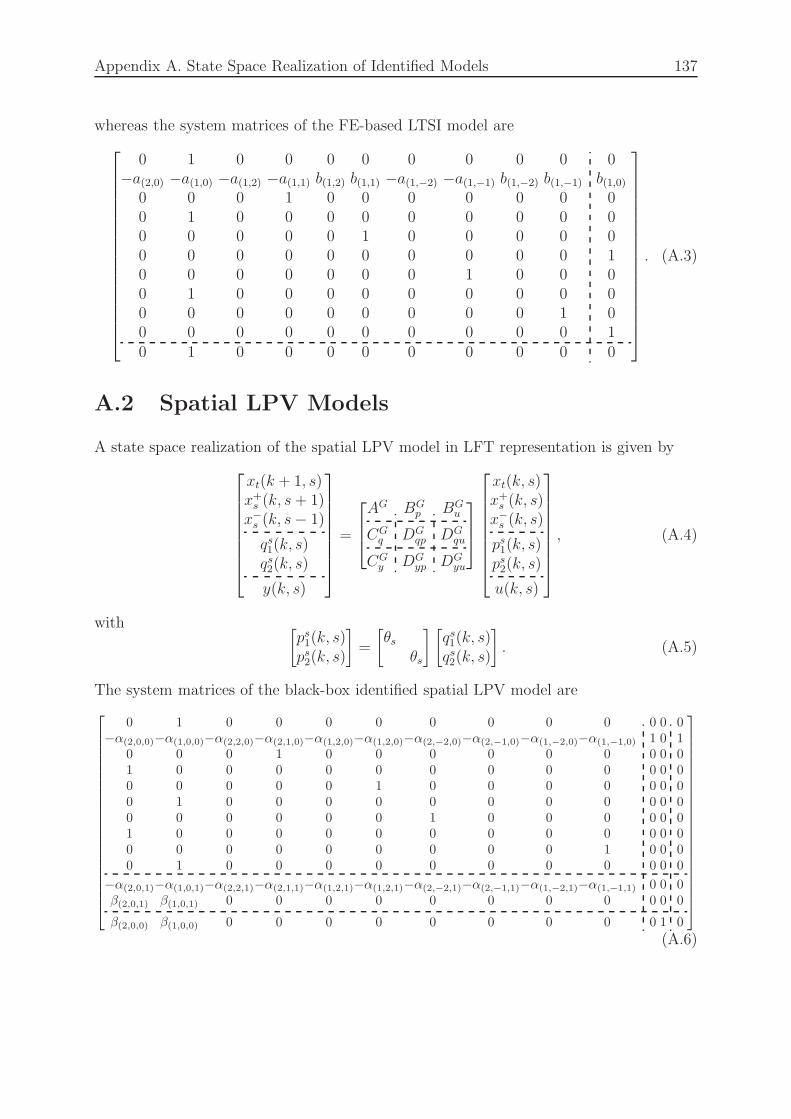
Appendix A. State Space Realization of Identified Models 137
whereas the system matrices of the FE-based LTSI model are
0 1 0 0 0 0 0 0 0 0 0−a(2,0) −a(1,0) −a(1,2) −a(1,1) b(1,2) b(1,1) −a(1,−2) −a(1,−1) b(1,−2) b(1,−1) b(1,0)
0 0 0 1 0 0 0 0 0 0 00 1 0 0 0 0 0 0 0 0 00 0 0 0 0 1 0 0 0 0 00 0 0 0 0 0 0 0 0 0 10 0 0 0 0 0 0 1 0 0 00 1 0 0 0 0 0 0 0 0 00 0 0 0 0 0 0 0 0 1 00 0 0 0 0 0 0 0 0 0 10 1 0 0 0 0 0 0 0 0 0
. (A.3)
A.2 Spatial LPV Models
A state space realization of the spatial LPV model in LFT representation is given by
xt(k + 1, s)x+s (k, s+ 1)
x−s (k, s− 1)
qs1(k, s)qs2(k, s)
y(k, s)
=
AG BGp BG
u
CGq DG
qp DGqu
CGy DG
yp DGyu
xt(k, s)x+s (k, s)
x−s (k, s)
ps1(k, s)ps2(k, s)
u(k, s)
, (A.4)
with [ps1(k, s)ps2(k, s)
]
=
[θs
θs
] [qs1(k, s)qs2(k, s)
]
. (A.5)
The system matrices of the black-box identified spatial LPV model are
0 1 0 0 0 0 0 0 0 0 0 0 0−α(2,0,0)−α(1,0,0)−α(2,2,0)−α(2,1,0)−α(1,2,0)−α(1,2,0)−α(2,−2,0)−α(2,−1,0)−α(1,−2,0)−α(1,−1,0) 1 0 1
0 0 0 1 0 0 0 0 0 0 0 0 01 0 0 0 0 0 0 0 0 0 0 0 00 0 0 0 0 1 0 0 0 0 0 0 00 1 0 0 0 0 0 0 0 0 0 0 00 0 0 0 0 0 1 0 0 0 0 0 01 0 0 0 0 0 0 0 0 0 0 0 00 0 0 0 0 0 0 0 0 1 0 0 00 1 0 0 0 0 0 0 0 0 0 0 0
−α(2,0,1)−α(1,0,1)−α(2,2,1)−α(2,1,1)−α(1,2,1)−α(1,2,1)−α(2,−2,1)−α(2,−1,1)−α(1,−2,1)−α(1,−1,1) 0 0 0β(2,0,1) β(1,0,1) 0 0 0 0 0 0 0 0 0 0 0
β(2,0,0) β(1,0,0) 0 0 0 0 0 0 0 0 0 1 0
(A.6)
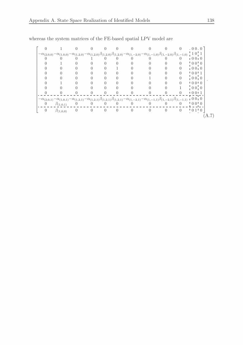
Appendix A. State Space Realization of Identified Models 138
whereas the system matrices of the FE-based spatial LPV model are
0 1 0 0 0 0 0 0 0 0 0 0 0−α(2,0,0)−α(1,0,0)−α(1,2,0)−α(1,2,0)β(1,2,0)β(1,2,0)−α(1,−2,0)−α(1,−1,0)β(1,−2,0)β(1,−1,0) 1 0 1
0 0 0 1 0 0 0 0 0 0 0 0 00 1 0 0 0 0 0 0 0 0 0 0 00 0 0 0 0 1 0 0 0 0 0 0 00 0 0 0 0 0 0 0 0 0 0 0 10 0 0 0 0 0 0 1 0 0 0 0 00 1 0 0 0 0 0 0 0 0 0 0 00 0 0 0 0 0 0 0 0 1 0 0 00 0 0 0 0 0 0 0 0 0 0 0 1
−α(2,0,1)−α(1,0,1)−α(1,2,1)−α(1,2,1)β(1,2,1)β(1,2,1)−α(1,−2,1)−α(1,−1,1)β(1,−2,1)β(1,−1,1) 0 0 00 β(1,0,1) 0 0 0 0 0 0 0 0 0 0 0
0 β(1,0,0) 0 0 0 0 0 0 0 0 0 1 0
.
(A.7)
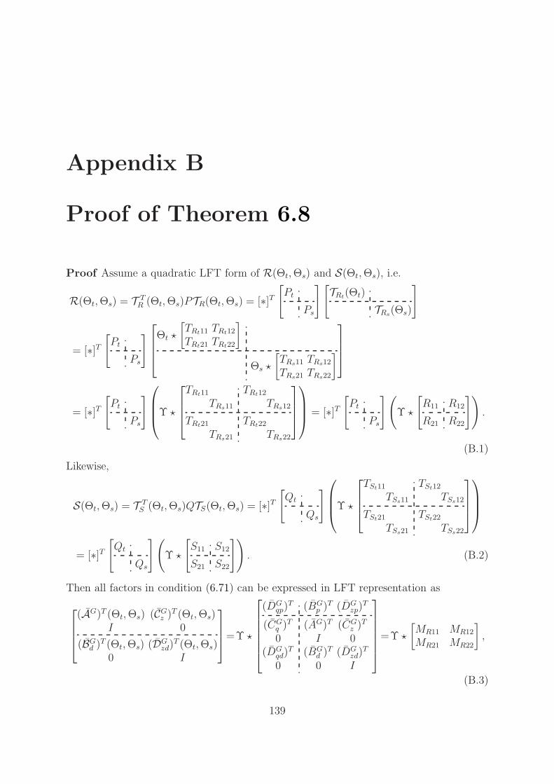
Appendix B
Proof of Theorem 6.8
Proof Assume a quadratic LFT form of R(Θt,Θs) and S(Θt,Θs), i.e.
R(Θt,Θs) = T TR (Θt,Θs)PTR(Θt,Θs) = [∗]T
[
Pt
Ps
][
TRt(Θt)
TRs(Θs)
]
= [∗]T[
Pt
Ps
]
Θt ⋆
[TRt11 TRt12
TRt21 TRt22
]
Θs ⋆
[TRs11 TRs12
TRs21 TRs22
]
= [∗]T[
Pt
Ps
]
Υ ⋆
TRt11 TRt12
TRs11 TRs12
TRt21 TRt22
TRs21 TRs22
= [∗]T[
Pt
Ps
](
Υ ⋆
[
R11 R12
R21 R22
])
.
(B.1)
Likewise,
S(Θt,Θs) = T TS (Θt,Θs)QTS(Θt,Θs) = [∗]T
[
Qt
Qs
]
Υ ⋆
TSt11 TSt12
TSs11 TSs12
TSt21 TSt22
TSs21 TSs22
= [∗]T[
Qt
Qs
](
Υ ⋆
[
S11 S12
S21 S22
])
. (B.2)
Then all factors in condition (6.71) can be expressed in LFT representation as
(AG)T (Θt,Θs) (CGz )
T (Θt,Θs)I 0
(BGd )
T (Θt,Θs) (DGzd)
T (Θt,Θs)0 I
=Υ ⋆
(DGqp)
T (BGp )
T (DGzp)
T
(CGq )
T (AG)T (CGz )
T
0 I 0(DG
qd)T (BG
d )T (DG
zd)T
0 0 I
=Υ ⋆
[MR11 MR12
MR21 MR22
]
,
(B.3)
139

Appendix B. Proof of Theorem 6.8 140
NR(Θt,Θs) = ker
(
Υ ⋆
[
(DGqp)
T (BGp )
T (DGzp)
T
(DGqu)
T (BGu )
T (DGzu)
T
])
= Υ ⋆
[NR11 NR12
NR21 NR22
]
, (B.4)
0 R(Θt,Θs) 0 0R(Θt,Θs) −∂R(Θt,Θs) 0 0
0 0 1γI 0
0 0 0 −γI
=[∗]T
0P 0 0P 0 0 00 0 1
γI 0
0 0 0 −γI
TR(Θt,Θs) −∂TR(Θt,Θs) 0 00 TR(Θt,Θs) 0 00 0 I 00 0 0 I
,
(B.5)
whose right factor is decomposed
TR(Θt,Θs) −∂TR(Θt,Θs) 0 00 TR(Θt,Θs) 0 00 0 I 00 0 0 I
=
∂ΥΥ
Υ
⋆
0 0 R11 0 R12 0 0R11 R11 0 −R12 0 0 00 0 R11 0 R12 0 0
−R21 −R21 0 R22 0 0 00 0 R21 0 R22 0 00 0 0 0 0 I 00 0 0 0 0 0 I
=
∂ΥΥ
Υ
⋆
[LR11 LR12
LR21 LR22
]
. (B.6)
Combine the LFT representations (B.3), (B.4) and (B.6). Condition (6.71) can be writtenas
[∗]T
0P 0 0P 0 0 00 0 1
γI 0
0 0 0 −γI
∂ΥΥ
Υ
⋆
[LR11 LR12
LR21 LR22
]
(
Υ ⋆
[MR11 MR12
MR21 MR22
])(
Υ ⋆
[NR11 NR12
NR21 NR22
])
< 0.
(B.7)After performing the star products, (B.7) becomes
[∗]T
0 P 0 0P 0 0 00 0 1
γI 0
0 0 0 −γI
∂ΥΥ
ΥΥ
Υ
⋆
[GP11 GP12
GP21 GP22
]
< 0, (B.8)
where
[
GP11 GP12
GP21 GP22
]
=
LR11 LR12MR21 LR12MR22NR21 LR12MR22NR22
0 MR11 MR12NR21 MR12NR22
0 0 NR11 NR12
LR21 LR22MR21 LR22MR22NR21 LR22MR22NR22
. (B.9)

Appendix B. Proof of Theorem 6.8 141
Applying similar procedures to (6.72) yields
[∗]T
0 Q 0 0Q 0 0 00 0 1
γI 0
0 0 0 −γI
∂ΥΥ
ΥΥ
Υ
⋆
[GQ11 GQ12
GQ21 GQ22
]
< 0, (B.10)
where
[
GQ11 GQ12
GQ21 GQ22
]
=
LS11 LS12MS21 LS12MS22NS21 LS12MS22NS22
0 MS11 MS12NS21 MS12NS22
0 0 NS11 NS12
LS21 LS22MS21 LS22MS22NS21 LS22MS22NS22
(B.11)
with
AG(Θt,Θs) BGd (Θt,Θs)
I 0CGz (Θt,Θs) DG
zd(Θt,Θs)0 I
= Υ ⋆
DGqp CG
q DGqd
BGp AG BG
d
0 I 0DG
zp CGz DG
zd
0 0 I
= Υ ⋆
[MS11 MS12
MS21 MS22
]
, (B.12)
NS(Θt,Θs) = ker
(
Υ ⋆
[
DGqp CG
p DGqd
DGyp CG
y DGyd
])
= Υ ⋆
[NS11 NS12
NS21 NS22
]
, (B.13)
and
0 S(Θt,Θs) 0 0S(Θt,Θs) ∂S(Θt,Θs) 0 0
0 0 1γI 0
0 0 0 −γI
=[∗]T
0 Q 0 0Q 0 0 00 0 1
γI 0
0 0 0 −γI
TS(Θt,Θs) ∂TS(Θt,Θs) 0 00 TS(Θt,Θs) 0 00 0 I 00 0 0 I
,
(B.14)
whose right factor is decomposed as
TS(Θt,Θs) ∂TS(Θt,Θs) 0 00 TS(Θt,Θs) 0 00 0 I 00 0 0 I
=
∂ΥΥ
Υ
⋆
0 0 S11 0 S12 0 0S11 S11 0 S12 0 0 00 0 S11 0 S12 0 0
S21 S21 0 S22 0 0 00 0 S21 0 S22 0 00 0 0 0 0 I 00 0 0 0 0 0 I
=
∂ΥΥ
Υ
⋆
[LS11 LS12
LS21 LS22
]
. (B.15)
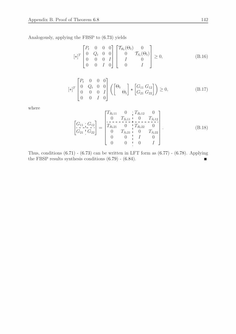
Appendix B. Proof of Theorem 6.8 142
Analogously, applying the FBSP to (6.73) yields
[∗]T
Pt 0 0 00 Qt 0 00 0 0 I0 0 I 0
TRt(Θt) 00 TSt
(Θt)I 00 I
≥ 0, (B.16)
[∗]T
Pt 0 0 00 Qt 0 00 0 0 I0 0 I 0
([Θt
Θt
]
⋆
[G11 G12
G21 G22
])
≥ 0, (B.17)
where
[
G11 G12
G21 G22
]
=
TRt11 0 TRt12 00 TSt11 0 TSt12
TRt21 0 TRt22 00 TSt21 0 TSt22
0 0 I 00 0 0 I
. (B.18)
Thus, conditions (6.71) - (6.73) can be written in LFT form as (6.77) - (6.78). Applyingthe FBSP results synthesis conditions (6.79) - (6.84).
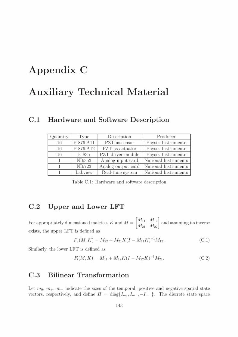
Appendix C
Auxiliary Technical Material
C.1 Hardware and Software Description
Quantity Type Description Producer16 P-876.A11 PZT as sensor Physik Instrumente16 P-876.A12 PZT as actuator Physik Instrumente16 E-835 PZT driver module Physik Instrumente1 NI6353 Analog input card National Instruments1 NI6723 Analog output card National Instruments1 Labview Real-time system National Instruments
Table C.1: Hardware and software description
C.2 Upper and Lower LFT
For appropriately dimensioned matricesK andM =
[M11 M12
M21 M22
]
and assuming its inverse
exists, the upper LFT is defined as
Fu(M,K) = M22 +M21K(I −M11K)−1M12. (C.1)
Similarly, the lower LFT is defined as
Fl(M,K) = M11 +M12K(I −M22K)−1M21. (C.2)
C.3 Bilinear Transformation
Let m0, m+, m− indicate the sizes of the temporal, positive and negative spatial statevectors, respectively, and define H = diagIm0
, Im+,−Im−
. The discrete state space
143
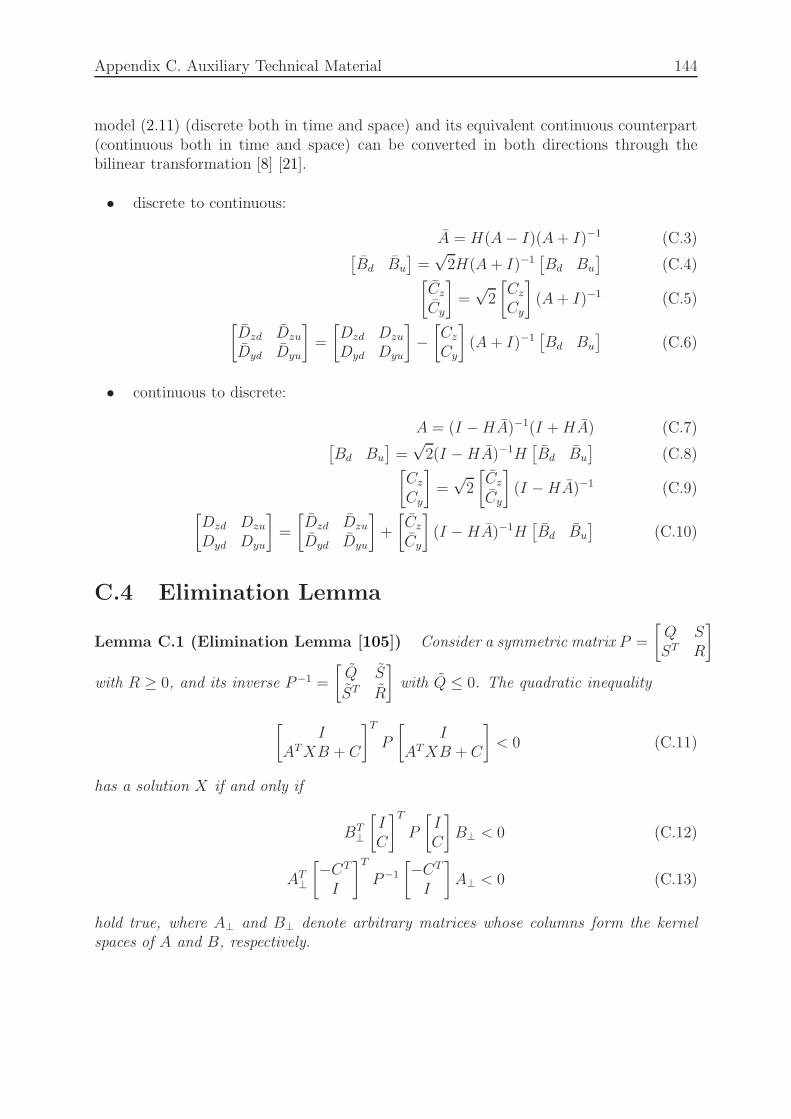
Appendix C. Auxiliary Technical Material 144
model (2.11) (discrete both in time and space) and its equivalent continuous counterpart(continuous both in time and space) can be converted in both directions through thebilinear transformation [8] [21].
• discrete to continuous:
A = H(A− I)(A+ I)−1 (C.3)[Bd Bu
]=
√2H(A+ I)−1
[Bd Bu
](C.4)
[Cz
Cy
]
=√2
[Cz
Cy
]
(A + I)−1 (C.5)
[Dzd Dzu
Dyd Dyu
]
=
[Dzd Dzu
Dyd Dyu
]
−[Cz
Cy
]
(A+ I)−1[Bd Bu
](C.6)
• continuous to discrete:
A = (I −HA)−1(I +HA) (C.7)[Bd Bu
]=
√2(I −HA)−1H
[Bd Bu
](C.8)
[Cz
Cy
]
=√2
[Cz
Cy
]
(I −HA)−1 (C.9)
[Dzd Dzu
Dyd Dyu
]
=
[Dzd Dzu
Dyd Dyu
]
+
[Cz
Cy
]
(I −HA)−1H[Bd Bu
](C.10)
C.4 Elimination Lemma
Lemma C.1 (Elimination Lemma [105]) Consider a symmetric matrix P =
[Q SST R
]
with R ≥ 0, and its inverse P−1 =
[Q S
ST R
]
with Q ≤ 0. The quadratic inequality
[I
ATXB + C
]T
P
[I
ATXB + C
]
< 0 (C.11)
has a solution X if and only if
BT⊥
[IC
]T
P
[IC
]
B⊥ < 0 (C.12)
AT⊥
[−CT
I
]T
P−1
[−CT
I
]
A⊥ < 0 (C.13)
hold true, where A⊥ and B⊥ denote arbitrary matrices whose columns form the kernelspaces of A and B, respectively.
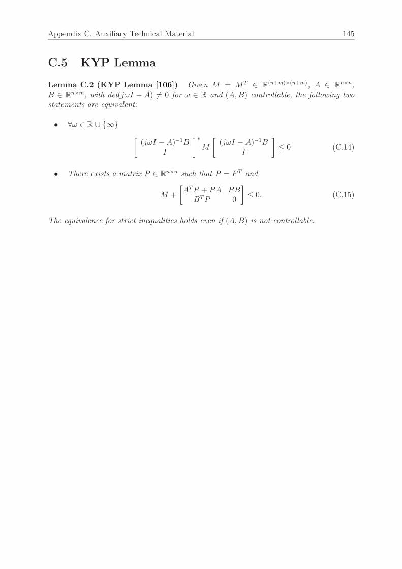
Appendix C. Auxiliary Technical Material 145
C.5 KYP Lemma
Lemma C.2 (KYP Lemma [106]) Given M = MT ∈ R(n+m)×(n+m), A ∈ Rn×n,B ∈ Rn×m, with det(jωI − A) 6= 0 for ω ∈ R and (A,B) controllable, the following twostatements are equivalent:
• ∀ω ∈ R ∪ ∞[(jωI −A)−1B
I
]∗
M
[(jωI −A)−1B
I
]
≤ 0 (C.14)
• There exists a matrix P ∈ Rn×n such that P = P T and
M +
[ATP + PA PB
BTP 0
]
≤ 0. (C.15)
The equivalence for strict inequalities holds even if (A,B) is not controllable.
Bibliography
[1] K. C. Chu, “Decentralized Control of High-Speed Vehicular Strings,” Transport.Sci., vol. 8, no. 4, pp. 361–384, 1974.
[2] G. E. Stewart, “Two-Dimensional Loop Shaping Controller Design for Paper Ma-chine Cross-directional Processes,” Dissertation, University of British Columbia,Vancouver, Canada, 2000.
[3] S. S. Chughtai and H. Werner, “Modeling and Distributed Control of Transitionin Plane Poiseuille Flow,” IEEE Trans. Contr. Syst. Technol., vol. 20, no. 3, pp.755–762, 2012.
[4] M. V. Gandhi and B. S. Thompson, Smart Materials and Structures, 1st ed.London and New York: Chapman & Hall, 1992.
[5] R. F. Curtain and H. J. Zwart, An Introduction to Infinite-Dimensional LinearSystems Theory, ser. Texts in Applied Mathematics. New York: Springer-Verlag,1995, vol. 21.
[6] B. Bamieh, F. Paganini, and M. A. Dahleh, “Distributed Control of SpatiallyInvariant Systems,” IEEE Trans. Automat. Contr., vol. 47, no. 7, pp. 1091–1107,2002.
[7] M. Jovanovic, “Modeling, Analysis, and Control of Spatially Distributed Systems,”Dissertation, University of California, Santa Barbara, CA, 2004.
[8] R. D’Andrea and G. E. Dullerud, “Distributed Control Design for Spatially Inter-connected Systems,” IEEE Trans. Automat. Contr., vol. 48, no. 9, pp. 1478–1495,2003.
[9] K. Napolitano and M. Schlosser, “Calculation of Rigid Body Mass Propertiesof Flexible Structures,” in Advanced Aerospace Applications, ser. ConferenceProceedings of the Society for Experimental Mechanics Series, T. Proulx, Ed.Springer, 2011.
[10] J. S. Shamma, “Analysis and Design of Gain Scheduled Control Systems,” Dis-sertation, Massachusetts Institute of Technology, 1988.
[11] P. Apkarian and P. Gahinet, “A Convex Characterization of Gain-Scheduled H∞Controllers,” IEEE Trans. Automat. Contr., vol. 40, no. 5, pp. 853–864, 1995.
146

BIBLIOGRAPHY 147
[12] P. Apkarian, P. Gahinet, and G. Becker, “Self-Scheduled H∞ Control of LinearParameter-varying Systems: a Design Example,” Automatica, vol. 31, no. 9, pp.1251–1261, 1995.
[13] P. Apkarian and R. J. Adams, “Advanced Gain-Scheduling Techniques for Un-certain Systems,” IEEE Trans. Contr. Syst. Technol., vol. 6, no. 1, pp. 21–32,1998.
[14] F. Wu and K. Dong, “Gain-Scheduling Control of LFT Systems Using Parameter-Dependent Lyapunov Functions,” Automatica, vol. 42, no. 1, pp. 39–50, 2006.
[15] P. Gahinet, P. Apkarian, and M. Chilali, “Affine Parameter-Dependent LyapunovFunctions and Real Parametric Uncertainty,” IEEE Trans. Automat. Contr.,vol. 41, no. 3, pp. 436–442, 1996.
[16] J. S. Shamma, “An Overview of LPV Systems,” in Control of Linear ParameterVarying Systems with Applications, J. Mohammadpour and C. W. Scherer, Eds.Springer US, 2012.
[17] C. Hoffmann and H. Werner, “A Survey of Linear Parameter-Varying Control Ap-plications Validated by Experiments or High-Fidelity Simulations,” IEEE Trans.Contr. Syst. Technol., vol. 23, no. 2, pp. 1–18, 2014.
[18] F. Wu, “Control of Linear Parameter Varying Systems,” Dissertation, Universityof Berkeley, Berkeley, CA, 1995.
[19] M. Dettori, “LMI Techniques for Control with Application to a Compact DiscPlayer Mechanism,” Dissertation, Delft University of Technology, Delft, Nether-lands, 2001.
[20] A. Helmersson, “Methods for Robust Gain-Scheduling,” Dissertation, LinkopingUniversity, Sweden, 1995.
[21] F. Wu, “Distributed Control for Interconnected Linear Parameter-Dependent Sys-tems,” IEE Proc., Control Theory Appl., vol. 150, no. 5, pp. 518–527, 2003.
[22] K.-J. Bathe, Finite Element Procedures. Upper Saddle River, NJ: Prentice Hall,1996.
[23] R. Holland and E. P. EerNisse, “Variational Evaluation of Admittances of Multi-electroded Three-Dimensional Piezoelectric Structures,” IEEE Trans. Son. Ultra-son., vol. 15, no. 2, pp. 119–131, 1968.
[24] H. Allik and Hughes, Thomas J. R., “Finite Element Method for PiezoelectricVibration,” Int. J. Numer. Meth. Engng., vol. 2, no. 2, pp. 151–157, 1970.
[25] G. L. C. M. d. Abreu, J. F. Ribeiro, and V. Steffen, Jr., “Finite Element Modelingof a Plate with Localized Piezoelectric Sensors and Actuators,” J. Braz. Soc. Mech.Sci. & Eng., vol. 26, no. 2, pp. 117–128, 2004.

BIBLIOGRAPHY 148
[26] M. Rios-Gutierrez and G. Silva-Navarro, “Finite Element and Modal Modeling ofa Cantilever Beam with Piezoelectric Patch Actuator for Vibration Absorption,”in Proc. 6th IEEE Conf. Elect. Eng., Computing Sci. and Automat. Control, 2009.
[27] M. Ali, S. S. Chughtai, and H. Werner, “Identification of Spatially InterconnectedSystems,” in Proc. 48th IEEE Conf. Decision Control, 2009.
[28] B. Bamieh and L. Giarre, “Identification of Linear Parameter Varying Models,”Int. J. Robust Nonlinear Contr., vol. 12, no. 9, pp. 841–853, 2002.
[29] M. Ali, S. S. Chughtai, and H. Werner, “Identification of LPV Models for SpatiallyVarying Interconnected Systems,” in Proc. Amer. Control Conf., 2010.
[30] J. K. Rice and M. Verhaegen, “Distributed Control: A Sequentially Semi-Separable Approach,” in Proc. 47th IEEE Conf. Decision Control, 2008.
[31] P. Massioni and M. Verhaegen, “Distributed Control for Identical DynamicallyCoupled Systems: A Decomposition Approach,” IEEE Trans. Automat. Contr.,vol. 54, no. 1, pp. 124–135, 2009.
[32] G. E. Stewart, D. M. Gorinevsky, and G. A. Dumont, “Feedback Controller Designfor a Spatially Distributed System: the Paper Machine Problem,” IEEE Trans.Contr. Syst. Technol., vol. 11, no. 5, pp. 612–628, 2003.
[33] E. Scholte and R. D’Andrea, “Active Vibro-Acoustic Control of a Flexible BeamUsing Distributed Control,” in Proc. Amer. Control Conf., 2003.
[34] G. E. Dullerud and R. D’Andrea, “Distributed Control of Heterogeneous Systems,”IEEE Trans. Automat. Contr., vol. 49, no. 12, pp. 2113–2128, 2004.
[35] J. Doyle and R. S. Smith, “Control of Plants with Input Saturation Nonlinearities,”in Proc. Amer. Control Conf. Proc. Amer. Control Conf., 1987.
[36] P. F. Weston and I. Postlethwaite, “Linear Conditioning for Systems ContainingSaturating Actuators,” Automatica, vol. 36, no. 9, pp. 1347–1354, 2000.
[37] G. Grimm, J. Hatfield, I. Postlethwaite, A. R. Teel, M. C. Turner, and L. Zaccar-ian, “Antiwindup for Stable Linear Systems with Input Saturation: An LMI-basedSynthesis,” IEEE Trans. Automat. Contr., vol. 48, no. 9, pp. 1509–1525, 2003.
[38] M. C. Turner, G. Herrmann, and I. Postlethwaite, “Incorporating RobustnessRequirements Into Antiwindup Design,” IEEE Trans. Automat. Contr., vol. 52,no. 10, pp. 1842–1855, 2007.
[39] E. F. Mulder, M. V. Kothare, and M. Morari, “Multivariable Anti-Windup Con-troller Synthesis Using Linear Matrix Inequalities,” Automatica, vol. 37, no. 9, pp.1407–1416, 2001.

BIBLIOGRAPHY 149
[40] M. Kishida and R. D. Braatz, “Robust Anti-Windup Compensation for NormalSystems with Application to the Reaction-Diffusion Equation,” in Proc. 18th IFACWorld Congr., 2011.
[41] Y. Li and M. Cantoni, “On Distributed Anti-Windup Compensation for Dis-tributed Linear Control Systems,” in Proc. 46th IEEE Conf. Decision Control,2007.
[42] A. Megretski and A. Rantzer, “System Analysis Via Integral Quadratic Con-straints,” IEEE Trans. Automat. Contr., vol. 42, no. 6, pp. 819–830, 1997.
[43] C. W. Scherer, “LPV Control and Full Block Multipliers,” Automatica, vol. 37,no. 3, pp. 361–375, 2001.
[44] K. Zhou, J. Doyle, and K. Glover, Robust and Optimal Control. Upper SaddleRiver, NJ: Prentice-Hall, 1996.
[45] C. W. Scherer, “Robust Mixed Control and LPV Control with Full Block Scal-ings.” Philadelphia, PA: SIAM.
[46] C. Galassi, Piezoelectric Materials: Advances in Science, Technology, and Ap-plications, ser. NATO science series. Series 3, High technology. Dordrecht andBoston: Kluwer Academic Publishers, 2000, vol. 76.
[47] H. Kawai, “The Piezoelectricity of Poly (vinylidene Fluoride),” Jpn. J. Appl.Phys., vol. 8, no. 7, pp. 975–976, 1969.
[48] Y. R. Wang, J. M. Zheng, G. Y. Ren, P. H. Zhang, and C. Xu, “A FlexiblePiezoelectric Force Sensor based on PVDF Fabrics,” Smart Mater. Struct., vol. 20,no. 4, p. 045009, 2011.
[49] IEEE Standard on Piezoelectricity. ANSI/IEEE Std 176-1987, 1988.
[50] PI, “P-876 Datasheet, DuraActTM Piezoelectric Patch Transducers.”
[51] A. Preumont, Vibration Control of Active Structures, An Introduction - 2nd Edi-tion, Dordrecht and Boston, 2002, vol. 96.
[52] W. B. Bickford, A First Course in the Finite Element Method, 2nd ed. BurrRidge, IL: Richard D Irwin, 1994.
[53] H. S. Tzou and C. I. Tseng, “Distributed Piezoelectric Sensor/Actuator Designfor Dynamic Measurement/Control of Distributed Parameter Systems: A Piezo-electric Finite Element Approach,” J. Sound Vib., vol. 138, no. 1, pp. 17–34, 1990.
[54] V. Piefort, “Finite Element Modelling of Piezoelectric Active Structures,” Disser-tation, Universite libre de Bruxelles, Brussel, Belgien, 2001.
[55] O. A. Bauchau and J. I. Craig, Structural analysis: With Applications to AerospaceStructures, ser. Solid Mechanics and its Applications. Dordrecht: Springer, 2009,vol. 163.

BIBLIOGRAPHY 150
[56] J. He and Z.-F. Fu,Modal Analysis. Oxford and Boston: Butterworth-Heinemann,2001.
[57] D. J. Ewins, Modal Testing: Theory, Practice, and Application, 2nd ed., ser. Me-chanical Engineering Research Studies: Engineering Dynamics Series. Baldock,Hertfordshire, England: Research Studies Press, 2000, vol. 10.
[58] D. W. Marquardt, “An Algorithm for Least-Squares Estimation of Nonlinear Pa-rameters,” SIAM J. Appl. Math., vol. 11, no. 2, pp. 431–441, 1963.
[59] D. F. Pilkey, “Computation of a Damping Matrix for Finite Element Model Up-dating,” Dissertation, Virginia Polytechnic Institute and State University, Blacks-burg, Virginia, 1998.
[60] Q. Liu, J. Gross, S. Pfeiffer, and H. Werner, “A Local Approach for the LPVIdentification of an Actuated Beam Using Piezoelectric Actuators and Sensors,”Mechatronics, vol. 24, no. 4, pp. 289–297, 2014.
[61] A. A. Khalate, X. Bombois, R. Toth, and R. Babuska, “Optimal ExperimentalDesign for LPV Identification Using a Local Approach,” in 15th IFAC Symp. Syst.Ident., 2009.
[62] M. Steinbuch, R. van de Molengraft, and A. van der Voort, “Experimental Mod-elling and LPV Control of a Motion System,” in Proc. Amer. Control Conf., 2003.
[63] R. Toth, “Modeling and Identification of Linear Parameter-Varying Systems, anOrthonormal Basis Function Approach,” Dissertation, Delft University of Tech-nology, Delft, Netherlands, 2008.
[64] H. Benaroya, Mechanical Vibration: Analysis, Uncertainties, and Control, 2nd ed.,ser. Mechanical Engineering. New York: Marcel Dekker, 2004, vol. 181.
[65] Q. Liu and H. Werner, “Experimental Identification of Spatially-InterconnectedParameter-Invariant and LPV Models for Actuated Beams,” in Proc. 52nd IEEEConf. Decision Control, 2013.
[66] Q. Liu, J. Gross, and H. Werner, “Distributed Identification of Spatially-Distributed Systems based on Finite Element Modelling,” in Proc. 54th IEEEConf. Decision Control, 2015.
[67] J. Crank and P. Nicolson, “A Practical Method for Numerical Evaluation of Solu-tions of Partial Differential Equations of the Heat-Conduction Type,” Adv ComputMath, vol. 6, no. 1, pp. 207–226, 1996.
[68] R. Courant, K. Friedrichs, and H. Lewy, “On the Partial Difference Equations ofMathematical Physics,” IBM J. Res. & Dev., vol. 11, no. 2, pp. 215–234, 1967.
[69] J. C. Strikwerda, Finite Difference Schemes and Partial Differential Equations,2nd ed. Philadelphia, PA: SIAM, 2004.
BIBLIOGRAPHY 151
[70] D. E. Dudgeon and R. M. Mersereau, Multidimensional Digital Signal Processing.Prentice-Hall Inc. USA, 1984.
[71] M. Ali, “Identification and Control of Spatially Interconnected Systems,” Disser-tation, Hamburg University of Technology, Hamburg, Germany, 2011.
[72] M. Ali, A. Ali, H. S. Abbas, and H. Werner, “Identification of Box-Jenkins Modelsfor Parameter-Varying Spatially Interconnected Systems,” in Proc. Amer. ControlConf., 2011.
[73] M. Ali, H. S. Abbas, S. S. Chughtai, and H. Werner, “Identification of Spatially In-terconnected Systems Using Neural Networks,” in Proc. 49th IEEE Conf. DecisionControl, 2010.
[74] R. Toth, P. Heuberger, and Van den Hof, P., “Asymptotically Optimal Orthonor-mal Basis Functions for LPV System Identification,” Automatica, vol. 45, no. 6,pp. 1359–1370, 2009.
[75] L. Herrmann, “Vibration of the Euler-Bernoulli Beam with Allowance for Damp-ings,” in Proc. World Congr. on Engineering, vol. 2. Newseood Ltd., InternationalAssociation of Engineers, 2008.
[76] J. K. Rice and M. Verhaegen, “Distributed Control: A Sequentially Semi-Separable Approach for Spatially Heterogeneous Linear Systems,” IEEE Trans.Automat. Contr., vol. 54, no. 6, pp. 1270–1283, 2009.
[77] M. Norgaard, O. Ravn, N. K. Poulsen, and L. K. Hansen, Neural Networks forModelling and Control of Dynamic Systems. London: Springer-Verlag, 2003.
[78] M. Meisami-Azad, J. Mohammadpour Velni, K. Hiramoto, and K. M. Grigori-adis, “Integrated Design of Large-Scale Collocated Structural System and ControlParameters Using a Norm Upper Bound Approach,” in Efficient Modeling andControl of Large-Scale Systems, J. Mohammadpour and K. M. Grigoriadis, Eds.Springer US, 2010.
[79] Q. Liu, C. Hoffmann, and H. Werner, “Distributed Control of Parameter-VaryingSpatially Interconnected Systems Using Parameter-Dependent Lyapunov Func-tions,” in Proc. Amer. Control Conf., 2013.
[80] Q. Liu, A. Mendez Gonzalez, and H. Werner, “Distributed Control of Spatially-Interconnected Parameter-Invariant and LPV Models for Actuated Beams,” inProc. Amer. Control Conf., 2014.
[81] M. Ali, H. S. Abbas, and H. Werner, “MIMO Controller Synthesis for LTI andLPV Systems Using Input-Output Models,” in Proc. 18th IFAC World Congr.,2011.
[82] S. Wollnack, H. S. Abbas, R. Toth, and H. Werner, “Fixed-Structure LPV Con-troller Synthesis Based on Implicit Input-Output Representations,” in Proc. 52ndIEEE Conf. Decision Control, 2013.

BIBLIOGRAPHY 152
[83] R. Toth, H. S. Abbas, and H. Werner, “On the State-Space Realization of LPVInput-Output Models: Practical Approaches,” IEEE Trans. Contr. Syst. Technol.,vol. 20, no. 1, pp. 139–153, 2012.
[84] C. W. Scherer, “Theory of Robust Control,” Lecture Notes, Delft University ofTechnology, Delft, Netherlands, 2001.
[85] G. E. Stewart, D. M. Gorinevsky, and G. A. Dumont, “Two-Dimensional LoopShaping,” Automatica, vol. 39, no. 5, pp. 779–792, 2003.
[86] R. D’Andrea, “Software for Modeling, Analysis, and Control Design for Multidi-mensional Systems,” in Proc. IEEE Int. Symposium Comput. Aid. Control Syst.Des., 1999.
[87] M. Dettori and C. W. Scherer, “LPV Design for a CD Player: an ExperimentalEvaluation of Performance,” in Proc. 40th IEEE Conf. Decision Control, 2001.
[88] S. P. Boyd, L. E. Ghaoui, E. Feron, and V. Balakrishnan, Linear Matrix Inequal-ities in System and Control Theory, ser. SIAM, 1994, vol. 15.
[89] G. Grimm, A. R. Teel, and L. Zaccarian, “Linear LMI-based External Anti-Windup Augmentation for Stable Linear Systems,” Automatica, vol. 40, no. 11,pp. 1987–1996, 2004.
[90] G. Li, W. P. Heath, and G. Herrmann, “Robust Anti-Windup Compensator Syn-thesis via Integral Quadratic Constraints,” in Proc. 18th IFAC World Congr.,vol. 18, 2011.
[91] R. M. Morales, G. Li, and W. P. Health, “Anti-Windup and the Preservation ofRobustness against Structured Norm-Bounded Uncertainty,” in Proc. 17th IFACWorld Congr., vol. 17, 2008.
[92] F. Wu, K. M. Grigoriadis, and A. K. Packard, “Anti-Windup Controller DesignUsing Linear Parameter-Varying Control Methods,” Int. J. Contr., vol. 73, no. 12,pp. 1104–1114, 2000.
[93] Q. Liu and H. Werner, “Distributed Antiwindup Compensation for Spatially-Interconnected Systems,” in Proc. Amer. Control Conf., 2015.
[94] M. C. Turner and D. Bates, Mathematical Methods for Robust and NonlinearControl: EPSRC Summer School, ser. Lecture Notes in Control and InformationSciences. Berlin and London: Springer, 2007.
[95] U. Jonssen, “Lecture Notes on Integral Quadratic Constraints,” Royal Instituteof Technology, Stockholm, Sweden, 2001.
[96] P. J. Seiler, A. Packard, and G. J. Balas, “A Dissipation Inequality Formulationfor Stability Analysis with Integral Quadratic Constraints,” in Proc. 49th IEEEConf. Decision Control, 2010.

BIBLIOGRAPHY 153
[97] H. Pfifer and P. J. Seiler, “Robust Analysis of Linear Parameter Varying SystemsUsing Integral Quadratic Constraints,” in Proc. Amer. Control Conf., 2014.
[98] M. C. Turner, G. Herrmann, and I. Postlethwaite, “Improving Sector-based Re-sults for Systems with Dead-Zone Nonlinearities and Constrained Control Appli-cations,” Automatica, vol. 45, no. 1, pp. 155–160, 2009.
[99] C. W. Scherer and I. E. Kose, “Robustness with Dynamic IQCs: An Exact State-Space Characterization of Nominal Stability with Applications to Robust Estima-tion,” Automatica, vol. 44, no. 7, pp. 1666–1675, 2008.
[100] C. W. Scherer, “Gain-Scheduled Synthesis with Dynamic Stable Strictly PositiveReal Multipliers: A Complete Solution,” in Proc. Europ. Control Conf., 2013.
[101] C. L. Beck, J. Doyle, and K. Glover, “Model Reduction of Multidimensional andUncertain Systems,” IEEE Trans. Automat. Contr., vol. 41, no. 10, pp. 1466–1477,1996.
[102] M. Ali, H. S. Abbas, and H. Werner, “Controller Synthesis for Input-Output LPVModels,” in Proc. Int. Conf. Control Applicat., 2010.
[103] S. Wollnack and H. Werner, “Distributed Fixed-Structure Control of SpatiallyInterconnected Systems,” in Proc. Amer. Control Conf., 2015.
[104] M. Vidyasagar, Nonlinear Systems Analysis, 2nd ed., ser. Classics in AppliedMathematics. Philadelphia, PA: SIAM, 2002.
[105] C. W. Scherer and S. Weiland, “Linear Matrix Inequalities in Control,” LectureNotes, Delft University of Technology, Delft, Netherlands, 2005.
[106] A. Rantzer, “On the Kalman–Yakubovich–Popov lemma,” Syst. Control Lett.,vol. 28, no. 1, pp. 7–10, 1996.
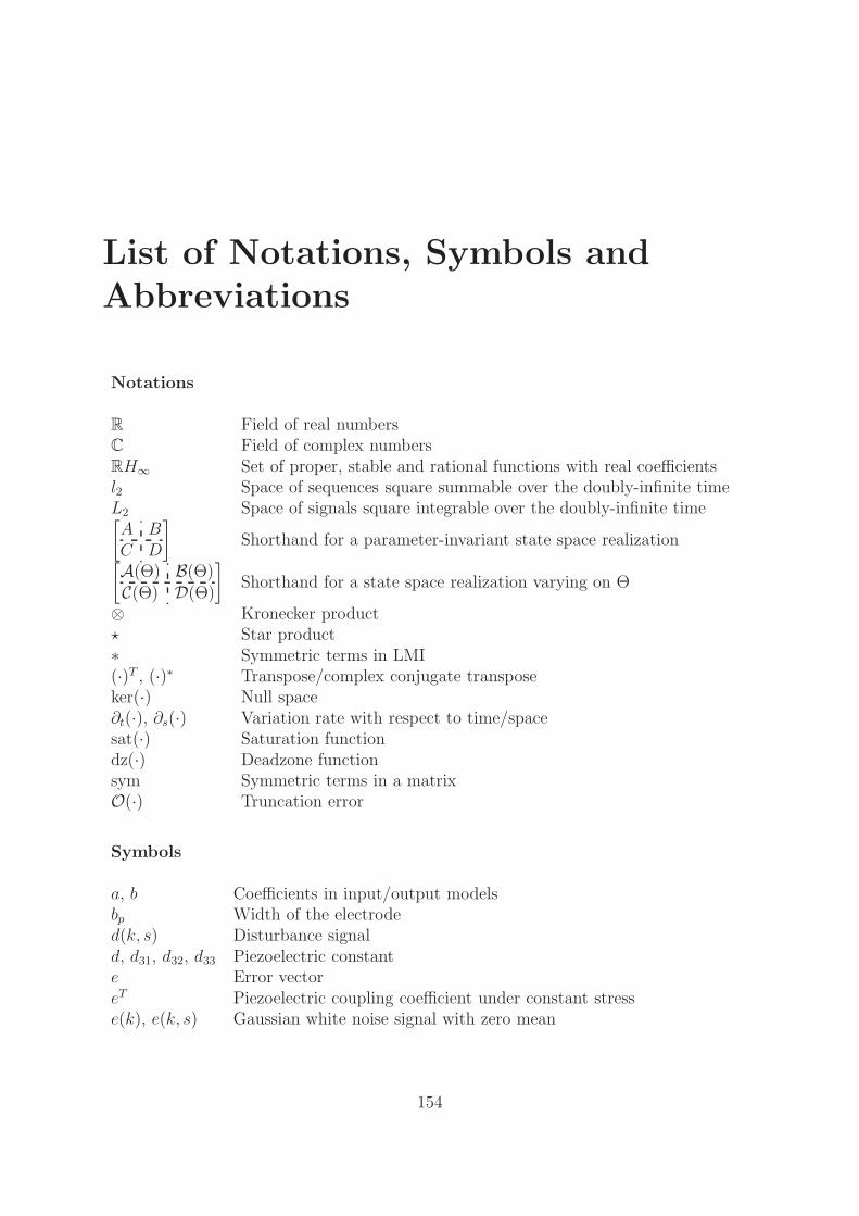
List of Notations, Symbols andAbbreviations
Notations
R Field of real numbersC Field of complex numbersRH∞ Set of proper, stable and rational functions with real coefficientsl2 Space of sequences square summable over the doubly-infinite timeL2 Space of signals square integrable over the doubly-infinite time[A BC D
]
Shorthand for a parameter-invariant state space realization[A(Θ) B(Θ)C(Θ) D(Θ)
]
Shorthand for a state space realization varying on Θ
⊗ Kronecker product⋆ Star product∗ Symmetric terms in LMI(·)T , (·)∗ Transpose/complex conjugate transposeker(·) Null space∂t(·), ∂s(·) Variation rate with respect to time/spacesat(·) Saturation functiondz(·) Deadzone functionsym Symmetric terms in a matrixO(·) Truncation error
Symbols
a, b Coefficients in input/output modelsbp Width of the electroded(k, s) Disturbance signald, d31, d32, d33 Piezoelectric constante Error vectoreT Piezoelectric coupling coefficient under constant stresse(k), e(k, s) Gaussian white noise signal with zero mean
154
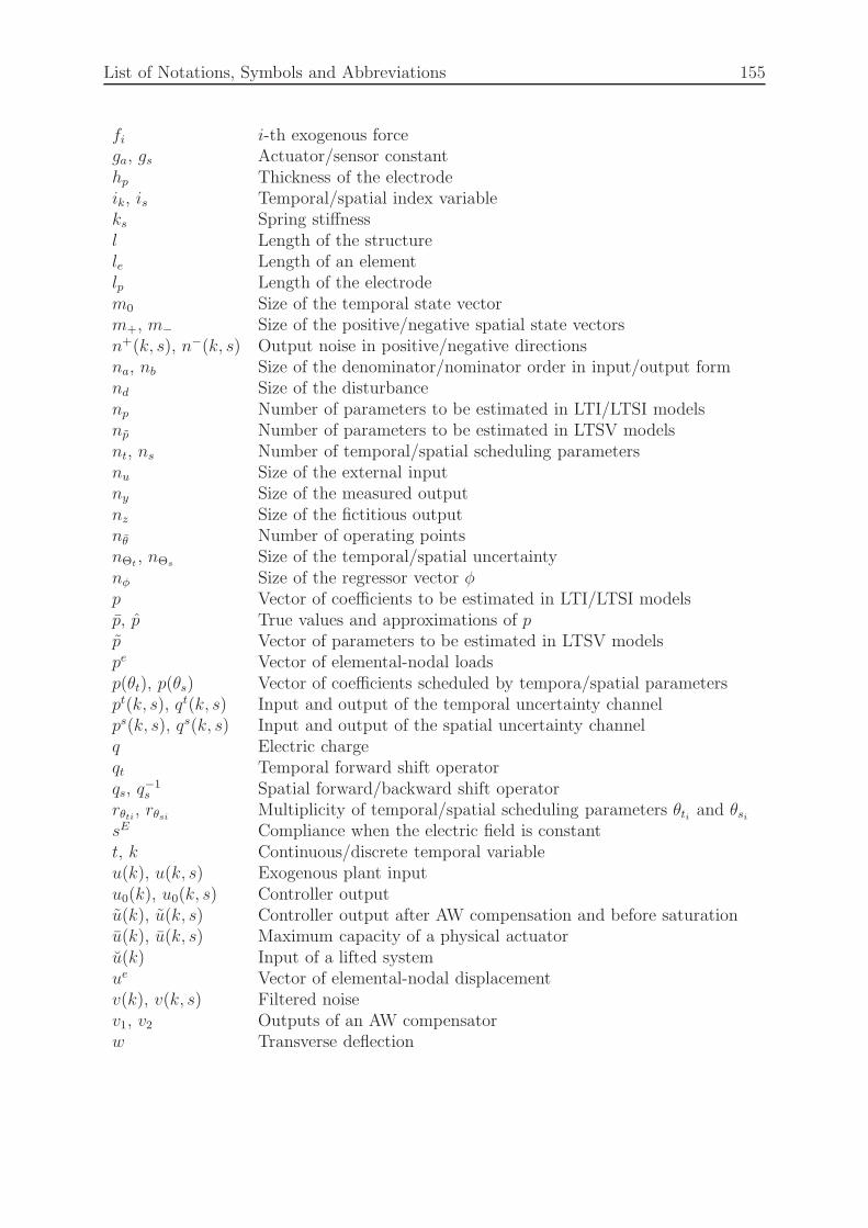
List of Notations, Symbols and Abbreviations 155
fi i-th exogenous forcega, gs Actuator/sensor constanthp Thickness of the electrodeik, is Temporal/spatial index variableks Spring stiffnessl Length of the structurele Length of an elementlp Length of the electrodem0 Size of the temporal state vectorm+, m− Size of the positive/negative spatial state vectorsn+(k, s), n−(k, s) Output noise in positive/negative directionsna, nb Size of the denominator/nominator order in input/output formnd Size of the disturbancenp Number of parameters to be estimated in LTI/LTSI modelsnp Number of parameters to be estimated in LTSV modelsnt, ns Number of temporal/spatial scheduling parametersnu Size of the external inputny Size of the measured outputnz Size of the fictitious outputnθ Number of operating pointsnΘt
, nΘsSize of the temporal/spatial uncertainty
nφ Size of the regressor vector φp Vector of coefficients to be estimated in LTI/LTSI modelsp, p True values and approximations of pp Vector of parameters to be estimated in LTSV modelspe Vector of elemental-nodal loadsp(θt), p(θs) Vector of coefficients scheduled by tempora/spatial parameterspt(k, s), qt(k, s) Input and output of the temporal uncertainty channelps(k, s), qs(k, s) Input and output of the spatial uncertainty channelq Electric chargeqt Temporal forward shift operatorqs, q
−1s Spatial forward/backward shift operator
rθti, rθsi Multiplicity of temporal/spatial scheduling parameters θti and θsisE Compliance when the electric field is constantt, k Continuous/discrete temporal variableu(k), u(k, s) Exogenous plant inputu0(k), u0(k, s) Controller outputu(k), u(k, s) Controller output after AW compensation and before saturationu(k), u(k, s) Maximum capacity of a physical actuatoru(k) Input of a lifted systemue Vector of elemental-nodal displacementv(k), v(k, s) Filtered noisev1, v2 Outputs of an AW compensatorw Transverse deflection

List of Notations, Symbols and Abbreviations 156
xt(k, s) Temporal statex+s (k, s) Spatial state in the positive direction
x−s (k, s) Spatial state in the negative direction
x(k) State of a lifted systemx, s Continuous/discrete spatial variabley(k), y(k, s) Measured output (controller input)y0(k), y0(k, s) Plant outputy(k), y(k, s) Estimated outputy(k) Output of a lifted systemz(k, s) Fictitious output
Ao Cross-section areaA(qt), A(qt, qs) Denominator polynomial of lumped or distributed modelsB(qt), B(qt, qs) Nominator polynomial of lumped or distributed modelsBu Derivative of shape function Nu
C Global damping matrixCa CapacitorCe Elemental damping matrixD Electric displacementE Young’s modulus
Electric fieldF Vector of exogenous forcesG(qt), G(qt, qs) Input/output representation of a plant modelG(s) Continuous transfer function of a plant modelH(qt), H(qt, qs) Input/output representation of a noise modelI Second moment of areaJ Cost functionK(qt) Discrete transfer function of a controllerKe
uφ, Keφu Mechanical and electrical coupled elemental stiffness matrix
Keuu Elemental mechanical-stiffness matrix
K Global stiffness matrixM Global mass matrixMe Elemental mass matrixMi i-th MomentMp Concentrated moment generated by Piezo actuatorMu, My Input/output maskNk, Ns Size of temporal/spatial measurementsNu Shape functionNR, NS Null spaceNR(·), NS(·) Parameter-varying null spaceP Global external loadP Matrix of estimated coefficients λQ Global electric chargeRe Resistance

List of Notations, Symbols and Abbreviations 157
S StrainS, S−1 Spatial forward/backward shift operatorT StressT Temporal forward shift operatorU Global mechanical variableV VolumeWf PostfilterWk Shaping filter of control sensitivityWs Shaping filter of sensitivityX Structured Lyapunov matrixXt, Xs Temporal/spatial Lyapunov matrixXm Set of structured Lyapunov matrix
Xm Set of structured Lyapunov matrix with only temporal componentsY Output vectorY Multiplier setZ Impedance
Greek Letter
α, β Parameters to be estimated in LTSV modelsγ Performance index∆m Augmented operator∆θ Matrix of exponents of operating points∆T Sampling time∆X Sampling spaceǫT Relative permittivity when the stress is constantη, H Regressor vector/matrix in LTSV model identificationθti , θsi Temporal/Spatial scheduling parameterθt, θs Vector of temporal/spatial scheduling parametersΘt, Θs Structured temporal/spatial uncertaintyΘt, Θs Compact set of structured temporal/spatial uncertaintyκ Curvatureλ Coefficients of polynomial functions on scheduling parametersΛ Matrix of polynomial coefficientsξ Dimensionless coordinateΞt, Ξs Set of the temporal/spatial variation rateΠ Multiplierρ Densityτ Vector of exponents of scheduling parametersΥ Augmented uncertainty
Υ Vertices of augmented uncertaintyφ, Φ Regressor vector/matrix in LTI or LTSI model identificationΦi, Φo Global input/output voltageφi, φo Elemental input/output voltage

List of Notations, Symbols and Abbreviations 158
ω FrequencyΩm, Ω Matrix of mode shapes
Superscript
G Plant modelK ControllerL Closed-loop system
L Permuted closed-loop system LP Closed-loop system including G, K, and Ψ
P Permuted closed-loop system PΨ AW compensator
Abbreviations
ARX AutoRegressive with eXogeneousAW AntiWindupBTCS Backward-Time Central-SpaceCFL Courant-Friedrichs-LewyCLF Constant Lyapunov FunctionCTCS Central-Time Central-SpaceDOF Degree of FreedomFBSP Full Block S-ProcedureFD Finite DifferenceFE Finite ElementFRF Frequency Response FunctionFTFS Forward-Time Forward-SpaceIQC Integral Quadratic ConstraintKYP Kalman-Yakubovic-PopovLFT Linear Fractional TransformationLMI Linear Matrix InequalityLPV Linear Parameter-VaryingLTI Linear Time-InvariantLTSI Linear Time- and Space-InvariantMEMS MicroElectroMechanical SystemMIMO Multiple-Input Multiple-OutputODE Ordinary Differential EquationPDE Partial Differential EquationPDLF Parameter-Dependent Lyapunov FunctionPI Physik InstrumentePVDF PolyVinylidene DiFluoridePZT Lead Zicronate TitanateSISO Single-Input Single-OutputSVD Singular Value Decomposition
List of Publications
Published
Q. Liu and H. Werner, Distributed Antiwindup Compensator for Spatially-InterconnectedSystems, in IEEE Proc. of American Control Conference, Chicago, USA, 2015
Q. Liu, A. Mendez, and H. Werner, Distributed Control of Spatially-InterconnectedParameter-Invariant and LPV Models for Actuated Beams, in IEEE Proc. of Ameri-can Control Conference, Portland, USA, 2014
G. Kaiser, M. Korte, Q. Liu, C. Hoffmann, and H. Werner, Torque Vectoring for a Real,Electric Car Implementing an LPV Controller, in 19th IFAC World Congress, Cape Town,South Africa, 2014
Q. Liu, J. Gross, S. Pfeiffer, and H. Werner, A Local Approach for the LPV Identificationof an Actuated Beam Using Piezoelectric Actuators and Sensors, in Mechatronics, vol.24, no. 4, pp. 289-297, Jun. 2014
Q. Liu and H. Werner, Experimental Identification of Spatially-Interconnected Parameter-Invariant and LPV Models for Actuated Beams, in 52nd IEEE Conference on Decisionand Control, Florence, Italy, 2013
Q. Liu, C. Hoffmann, and H. Werner, Distributed Control of Parameter-Varying SpatiallyInterconnected Systems Using Parameter-Dependent Lyapunov Functions, in IEEE Proc.of American Control Conference, Washington D.C., USA, 2013
M. Bartels, Q. Liu, G. Kaiser, and H. Werner, LPV Torque Vectoring for an ElectricVehicle Using Parameter-Dependent Lyapunov Functions, in IEEE Proc. of AmericanControl Conference, Washington D.C., USA, 2013
G. Kaiser, Q. Liu, and H. Werner, Torque Vectoring for an Electric Vehicle Using an LPVDrive Controller and a Torque and Slip Limiter, in 51st IEEE Conference on Decisionand Control, Hawaii, USA, 2012
159

List of Publications 160
Q. Liu, G. Kaiser, S. Boonto, H. Werner, F. Holzmann, B. Chretien and M. Korte,Two-Degree-of-Freedom LPV Control for a through-the-Road Hybrid Electric Vehicle viaTorque Vectoring, in 50th IEEE Conference on Decision and Control, Orlando, USA, 2011
Accepted
Q. Liu, J. Gross and H. Werner, Distributed Identification of Spatially-Distributed Sys-tems Based on Finite Element Modelling, in 54th IEEE Conference on Decision andControl, Osaka, Japan, 2015
Submitted
J. Gross, Q. Liu, M. Gomse and U. Weltin, Eigenpath Tracking in a Two-DimensionalNormal Modes Problem Using the Spectral Element Method and the Modal AssuranceCriterion, submitted to Journal of Sound and Vibration, 2015
Copyright © 2022 FDOKUMEN