arX

iv:p

hysi

cs/9

9110

73v2

[ph

ysic

s.op

tics]

28

Feb

2000

Polarized Electromagnetic Radiation fromSpatially Correlated Sources

Abhishek Agarwal1, Pankaj Jain2 and Jagdish Rai

Physics DepartmentIndian Institute of Technology

Kanpur, India 208016

Abstract

We consider the effect of spatial correlations on sources of polarized electromagnetic radiation. The

sources, assumed to be monochromatic, are constructed out of dipoles aligned along a line such that their

orientation is correlated with their position. In one representative example, the dipole orientations are

prescribed by a generalized form of the standard von Mises distribution for angular variables such that

the azimuthal angle of dipoles is correlated with their position. In another example the tip of the dipole

vector traces a helix around the symmetry axis of the source, thereby modelling the DNA molecule. We

study the polarization properties of the radiation emitted from such sources in the radiation zone. For

certain ranges of the parameters we find a rather striking angular dependence of polarization. This may

find useful applications in certain biological systems as well as in astrophysical sources.

1 Motivation

In a series of interesting papers Wolf [1, 2, 3] studied the spectrum of light from spatially correlated sourcesand found, remarkably, that in general the spectrum does not remain invariant under propagation eventhrough vacuum. The phenomenon was later confirmed experimentally [4, 5, 6] and has been a subject ofconsiderable interest [7]. Further investigations of the source correlation effects have been done in the timedomain theoretically [8] and experimentally [9]. Several applications of the effect have also been proposed[10, 11, 12, 13, 14]. In a related development it has been pointed out that spectral changes also arise dueto static scattering [15, 16, 17, 18, 19] and dynamic scattering [20, 21, 22, 23, 24]. In the present paper weinvestigate polarization properties of spatially correlated sources. Just as we expect spectral shifts for suchsources, we expect nontrivial polarization effects if the correlated source emits polarized light.

The basic idea can be illustrated by considering two polarized point sources P1 and P2 which are locatedalong the z-axis at a distance 2z apart, in analogy to a similar situation considered by Wolf [2] for theunpolarized case. The electric field at the point Q located at large distances R1 and R2 from these pointsources can be written as,

~E = ~e(~r1, ω)eikR1

R1+ ~e(~r2, ω)

eikR2

R2(1)

Here ~r1 and ~r2 are the position vectors of the points P1 and P2. We calculate the coherency matrix for thiselectric field at the point Q,

< E∗

i Ej > =< e∗i (~r1, ω)ej(~r1, ω) >

R21

+< e∗i (~r2, ω)ej(~r2, ω) >

R22

+

(

< e∗i (~r1, ω)ej(~r2, ω) > eik(R2−R1)

R1R2+ h.c.

)

(2)

We are interested in investigating the effect of the third term which arises due to cross correlation betweenthe sources P1 and P2. It is clear that this term will give nontrivial contribution to the polarization in the farzone. In the present paper we investigate the contribution of this term by considering only monochromaticwaves. It turns out to be useful to understand this simple idealization before treating the realistic case ofpartially polarized radiation.

In order to illustrate the contribution of the cross correlation term we consider the situation where thetwo sources are simple dipoles, ~p1 and ~p2 located at z and −z respectively and are oriented such that their

1current address: Physics Department, University of Rochester, Rochester, NY2e-mail: pkjain@iitk.ac.in

1

polar angles θ1 = θ2 = θp and the azimuthal angles φ1 = −φ2 = π/2. We assume that θp lies between 0and π/2. The strength of the dipoles is p0 and they radiate at frequency ω. We compute the electric fieldat point Q located at coordinates (R, θ, φ), as shown in Fig. 1, such that R >> z. The electric field in thefar zone is obtained by the addition of two vectors p1 · RR − p1 and p2 · RR − p2 with phase difference of2ωz cos θ/c. The vector p · RR− p at any point (R, θ, φ) is ofcourse simply the projection of the polarizationvector p on the plane perpendicular to R at that point. We keep only the leading order terms in z/R incomputing the total electric field.

The observed polarization is obtained by calculating the coherency matrix, given by

J =

( 〈EθE∗

θ 〉 〈EθE∗

φ〉〈E∗

φEθ〉 〈EφE∗

φ〉

)

(3)

The state of polarization can be uniquely specified by the Stokes’s parameters or equivalently the Poincaresphere variables [28]. The Stoke’s parameters are obtained in terms of the elements of the coherency matrixas: S0 = J11 + J22, S1 = J11 − J22, S2 = J12 + J21, S3 = i(J21 − J12). The parameter S0 is proportionalto the intensity of the beam. The Poincare sphere is charted by the angular variables 2χ, and 2ψ, which canbe expressed as:

S1 = S0 cos 2χ cos 2ψ, S2 = S0 cos 2χ sin 2ψ, S3 = S0 sin 2χ (4)

The angle χ (−π/4 ≤ χ ≤ π/4) measures of the ellipticity of the state of polarization and ψ (0 ≤ ψ < π)measures alignment of the linear polarization. For example, χ = 0 represents pure linear polarization andχ = π/4 pure right circular polarization.

The Stokes parameters at the observation point Q for the two dipole source are given by

S0 =

(

ω2p0

c2R

)2[

4 cos2(ωz cos θ/c) cos2 θp sin2 θ + 4 sin2(ωz cos θ/c) sin2 θp(cos2 θ sin2 φ+ cos2 φ)]

S1 =

(

ω2p0

c2R

)2[

4 cos2(ωz cos θ/c) cos2 θp sin2 θ + 4 sin2(ωz cos θ/c) sin2 θp(cos2 θ sin2 φ− cos2 φ)]

S2 =

(

ω2p0

c2R

)2

8 sin2(ωz cos θ/c) sin2 θp cos θ sinφ cosφ

S3 =

(

ω2p0

c2R

)2

8 cos(ωz cos θ/c) sin(ωz cos θ/c) cos θp sin θp sin θ cosφ

The resulting polarization in the far zone is quite interesting. At sinφ = 0, θ = π/2 the wave is linearlypolarized (χ = 0) with ψ = 0. As θ decreases from π/2 to 0, χ > 0 and the wave has general ellipticalpolarization with ψ = 0. At a certain value of the polar angle θ = θt the wave is purely right circularlypolarized. As θ crosses θt, the linearly polarized component jumps from 0 to π/2, i.e. 2ψ changes from 0 toπ. The value of the polar angle θt at which the transition occurs is determined by

tan(ωz cos θt/c) = ± sin θt/ tan θp (5)

From this equation we see that as z → 0, the transition angle θt is close to zero for a wide range of values ofθp. Only when θp → π/2, a solution with θt significantly different from 0 can be found. In general, however,we can find a solution with any value of θt by appropriately adjusting z and θp. For sinφ > 0, we findqualitatively similar results, except that now the linear polarization angle 2ψ increases smoothly from 0 asθ goes from π/2 to 0. Furthermore the state of polarization never becomes purely circular, i.e. the angle 2χis never equal to π/2 although it does achieve a maxima at θ close to the transition angle θt given by Eq. 5.

We therefore find that for wide range of parameters the polarization in the far field region shows anontrivial dependence on angular position which is governed by the cross correlation term. In general thisterm will give nontrivial contribution unless the two sources have identical polarizations.

2

y

z

x

O

R

Q(R,θ,φ)

p

θ

φ

Figure 1: The correlated source consisting of an array of dipoles aligned along the z axis. The observationpoint Q is at a distance R which is much larger than the spatial extent of the source.

2 A One Dimensional Spatially Correlated Source

A simple continuous model of a monochromatic spatially correlated source can be constructed by arranginga series of dipoles along a line with their orientations correlated with the position of the source. The dipoleswill be taken to be aligned along the z axis and distributed as a gaussian exp[−z2/2σ2]. The orientation ofthe dipole is characterized by the polar coordinates θp, φp, which are also assumed to be correlated with theposition z. A simple correlated ansatz is given by

exp [α cos(θp) + βz sin(φp)]

N1(α)N2(βz)(6)

where α and β are parameters, N1(α) = πI0(α) and N2(βz) = 2πI0(βz) are normalization factors andI0 is the Bessel function. The basic distribution function exp(α cos(θ − θ0)) used in the above ansatz isthe well known von Mises distribution which for circular data is in many ways the analoque of Gaussiandistribution for linear data [25, 26, 27]. For α > 0 this function peaks at θ = θ0. Making a Taylorexpansion close to its peak we find a gaussian distribution to leading power in θ − θ0. The maximumlikelihood estimators for the mean angle θ0 and the width parameter α are given by, < sin(θ− θ0) >= 0 and< cos(θ − θ0) >= d log(I0(α))/dα respectively. In prescribing the ansatz given in Eq. 6 we have assumedthat the polar angle θp of the dipole orientation is uncorrelated with z and the distribution is peaked eitherat θp = 0 (π) for α > 0 (< 0). The azimuthal angle φp is correlated with z such that for β > 0 and z > 0(< 0)the distribution peaks at φp = π/2(3π/2).

We next calculate the electric field at very large distance from such a correlated source. The observationpoint Q is located at the position (R, θ, φ) (Fig 1), measured in terms of the spherical polar coordinates, andwe assume that the spatial extent of the source σ << R. The electric field from such a correlated source atlarge distances is given by,

E = − ω2

c2Rp0e

i(−ωt+Rω/c)

∫

∞

−∞

dz exp(

−z2/2σ2)

∫ π

0

dθp

∫ 2π

0

dφp

3

× exp (α cos θp + βz sinφp)

2π2I0(α)I0(βz)exp

(

iωzR · z/c)

× (p · RR− p) (7)

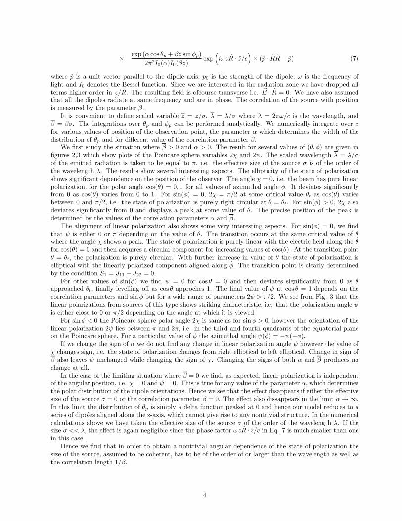
where p is a unit vector parallel to the dipole axis, p0 is the strength of the dipole, ω is the frequency oflight and I0 denotes the Bessel function. Since we are interested in the radiation zone we have dropped allterms higher order in z/R. The resulting field is ofcourse transverse i.e. ~E · R = 0. We have also assumedthat all the dipoles radiate at same frequency and are in phase. The correlation of the source with positionis measured by the parameter β.

It is convenient to define scaled variable z = z/σ, λ = λ/σ where λ = 2πω/c is the wavelength, andβ = βσ. The integrations over θp and φp can be performed analytically. We numerically integrate over zfor various values of position of the observation point, the parameter α which determines the width of thedistribution of θp and for different value of the correlation parameter β.

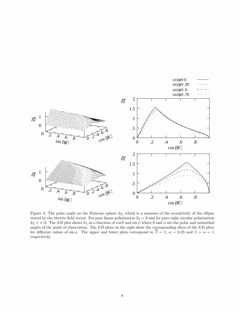
We first study the situation where β > 0 and α > 0. The result for several values of (θ, φ) are given infigures 2,3 which show plots of the Poincare sphere variables 2χ and 2ψ. The scaled wavelength λ = λ/σof the emitted radiation is taken to be equal to π, i.e. the effective size of the source σ is of the order ofthe wavelength λ. The results show several interesting aspects. The ellipticity of the state of polarizationshows significant dependence on the position of the observer. The angle χ = 0, i.e. the beam has pure linearpolarization, for the polar angle cos(θ) = 0, 1 for all values of azimuthal angle φ. It deviates significantlyfrom 0 as cos(θ) varies from 0 to 1. For sin(φ) = 0, 2χ = π/2 at some critical value θt as cos(θ) variesbetween 0 and π/2, i.e. the state of polarization is purely right circular at θ = θt. For sin(φ) > 0, 2χ alsodeviates significantly from 0 and displays a peak at some value of θ. The precise position of the peak isdetermined by the values of the correlation parameters α and β.

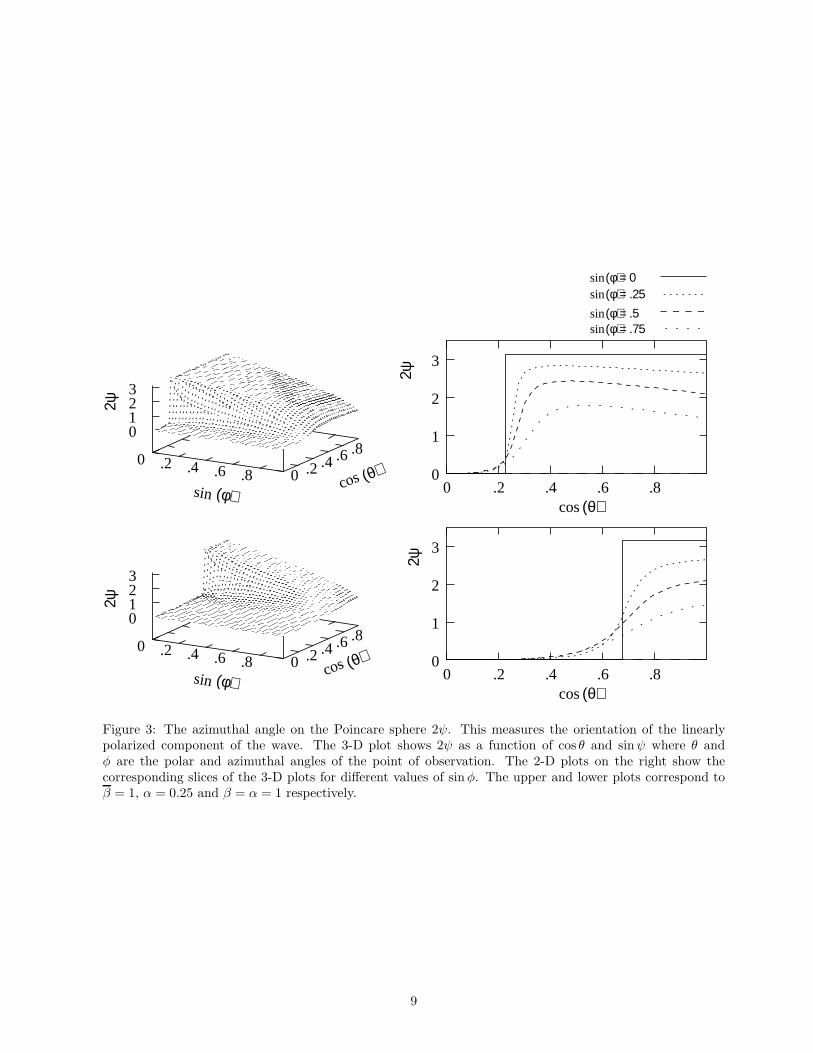
The alignment of linear polarization also shows some very interesting aspects. For sin(φ) = 0, we findthat ψ is either 0 or π depending on the value of θ. The transition occurs at the same critical value of θwhere the angle χ shows a peak. The state of polarization is purely linear with the electric field along the θfor cos(θ) = 0 and then acquires a circular component for increasing values of cos(θ). At the transition pointθ = θt, the polarization is purely circular. With further increase in value of θ the state of polarization iselliptical with the linearly polarized component aligned along φ. The transition point is clearly determinedby the condition S1 = J11 − J22 = 0.

For other values of sin(φ) we find ψ = 0 for cos θ = 0 and then deviates significantly from 0 as θapproached θt, finally levelling off as cos θ approches 1. The final value of ψ at cos θ = 1 depends on thecorrelation parameters and sinφ but for a wide range of parameters 2ψ > π/2. We see from Fig. 3 that thelinear polarizations from sources of this type shows striking characteristic, i.e. that the polarization angle ψis either close to 0 or π/2 depending on the angle at which it is viewed.

For sinφ < 0 the Poincare sphere polar angle 2χ is same as for sinφ > 0, however the orientation of thelinear polarization 2ψ lies between π and 2π, i.e. in the third and fourth quadrants of the equatorial planeon the Poincare sphere. For a particular value of φ the azimuthal angle ψ(φ) = −ψ(−φ).

If we change the sign of α we do not find any change in linear polarization angle ψ however the value ofχ changes sign, i.e. the state of polarization changes from right elliptical to left elliptical. Change in sign ofβ also leaves ψ unchanged while changing the sign of χ. Changing the signs of both α and β produces nochange at all.

In the case of the limiting situation where β = 0 we find, as expected, linear polarization is independentof the angular position, i.e. χ = 0 and ψ = 0. This is true for any value of the parameter α, which determinesthe polar distribution of the dipole orientations. Hence we see that the effect disappears if either the effectivesize of the source σ = 0 or the correlation parameter β = 0. The effect also dissappears in the limit α→ ∞.In this limit the distribution of θp is simply a delta function peaked at 0 and hence our model reduces to aseries of dipoles aligned along the z-axis, which cannot give rise to any nontrivial structure. In the numericalcalculations above we have taken the effective size of the source σ of the order of the wavelength λ. If thesize σ << λ, the effect is again negligible since the phase factor ωzR · z/c in Eq. 7 is much smaller than onein this case.

Hence we find that in order to obtain a nontrivial angular dependence of the state of polarization thesize of the source, assumed to be coherent, has to be of the order of or larger than the wavelength as well asthe correlation length 1/β.

4

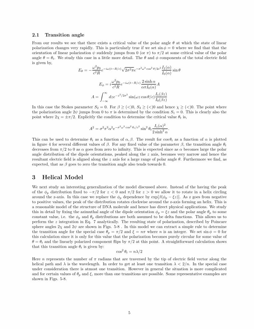
2.1 Transition angle

From our results we see that there exists a critical value of the polar angle θ at which the state of linearpolarization changes very rapidly. This is particularly true if we set sinφ = 0 where we find that that theorientation of linear polarization ψ suddenly jumps from 0 (or π) to π/2 at some critical value of the polarangle θ = θt. We study this case in a little more detail. The θ and φ components of the total electric fieldis given by,

Eθ = −ω2p0

c2Re−iω(t−R/c)

√2σ2πe−σ2ω2 cos2 θ/2c2 I1(α)

I0(α)sin θ

Eφ = iω2p0

c2Re−iω(t−R/c) 2 sinhα

απI0(α)A

A =

∫

∞

−∞

dze−z2/2σ2

sin(ωz cos θ/c)I1(βz)

I0(βz)

In this case the Stokes parameter S2 = 0. For β ≥ (<)0, S3 ≥ (<)0 and hence χ ≥ (<)0. The point wherethe polarization angle 2ψ jumps from 0 to π is determined by the condition S1 = 0. This is clearly also thepoint where 2χ = ±π/2. Explicitly the condition to determine the critical value θt is,

A2 = σ2π3α2e−σ2ω2 cos2 θt/c2

sin2 θtI1(α)2

2 sinh2 α.

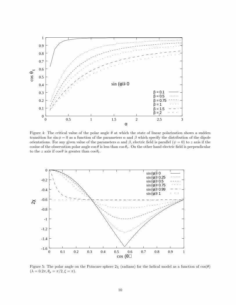
This can be used to determine θt as a function of α, β. The result for cos θt as a function of α is plottedin figure 4 for several different values of β. For any fixed value of the parameter β, the transition angle θt

decreases from π/2 to 0 as α goes from zero to infinity. This is expected since as α becomes large the polarangle distribution of the dipole orientations, peaked along the z axis, becomes very narrow and hence theresultant electric field is aligned along the z axis for a large range of polar angle θ. Furthermore we find, asexpected, that as β goes to zero the transition angle also tends towards 0.

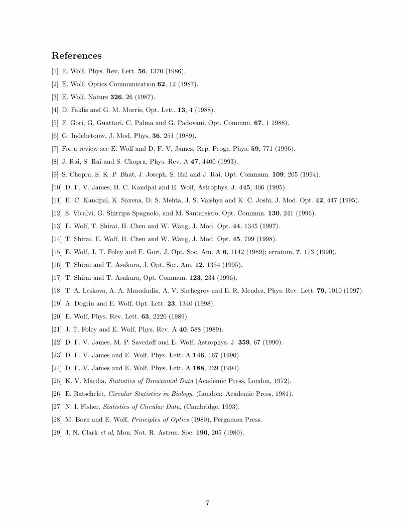
3 Helical Model

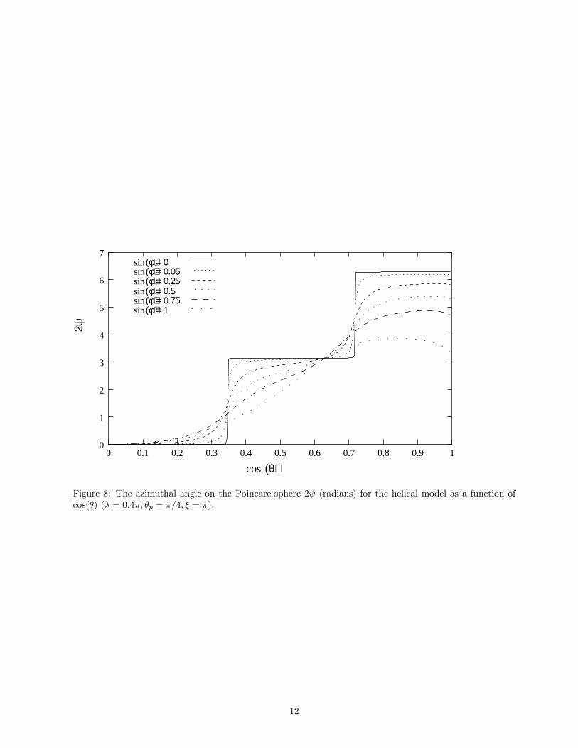
We next study an interesting generalization of the model discussed above. Instead of the having the peakof the φp distribution fixed to −π/2 for z < 0 and π/2 for z > 0 we allow it to rotate in a helix circlingaround the z-axis. In this case we replace the φp dependence by exp[β(φp − ξz)]. As z goes from negativeto positive values, the peak of the distribution rotates clockwise around the z-axis forming an helix. This isa reasonable model of the structure of DNA molecule and hence has direct physical applications. We studythis in detail by fixing the azimuthal angle of the dipole orientation φp = ξz and the polar angle θp to someconstant value, i.e. the φp and θp distributions are both assumed to be delta functions. This allows us toperform the z integration in Eq. 7 analytically. The resulting state of polarization, described by Poincaresphere angles 2χ and 2ψ are shown in Figs. 5-8 . In this model we can extract a simple rule to determinethe transition angle for the special case θp = π/2 and ξ = nπ where n is an integer. We set sinφ = 0 forthis calculation since it is only for this value that the polarization becomes purely circular for some value ofθ = θt and the linearly polarized component flips by π/2 at this point. A straightforward calculation showsthat this transition angle θt is given by:

cos2 θt = nλ/2

Here n represents the number of π radians that are traversed by the tip of electric field vector along thehelical path and λ is the wavelength. In order to get at least one transition λ < 2/n. In the special caseunder consideration there is atmost one transition. However in general the situation is more complicatedand for certain values of θp and ξ, more than one transitions are possible. Some representative examples areshown in Figs. 5-8.

5

4 Conclusions

In this paper we have considered spatially correlated monochromatic sources. We find that at large distancethe polarization of the wave shows dramatic dependence on the angular position of the observer. For certainset of parameters the linearly polarized component shows a sudden jump by π/2. If the symmetry axisof the source is taken to be the z-axis, the polarization shows a sudden transition from being parallelto perpendicular to the symmetry axis of the source, as the polar angle is changed from π/2 to 0. Thesources considered in this paper are idealized since we have assumed coherence over the entire source.For small enough sources, such as the DNA molecule, this may a reasonable approximation. In the case ofmacroscopic sources, this assumption is in general not applicable. However in certain situations some aspectsof the behavior described in this paper may survive even for these cases. For example, we may consider amacroscopic source consisting of large number of structures of the type considered in this paper. As long asthere is some correlation between the orientation of these structures over large distances we expect that someaspects of the angular dependence of the polarization of the small structures will survive, even if there doesnot exist any coherent phase relationship over large distances. Hence the ideas discussed in this paper mayalso find interesting applications to macroscopic and astrophysical sources. As an interesting example weconsider astrophysical sources of radio waves. It is well known that the polarization angle of these sources ispredominantly observed to be aligned either parallel or perpendicular to the source orientation axis [29]. Thisdifference has generally been attributed to the existence of different physical mechanism for the generation ofradio waves in these sources. Our study, however, indicates that this difference in observed polarization anglecould also arise simply due to different angles of observation. Hence orientation effects must be consideredbefore attributing different physical mechanisms for differences in observed polarizations of these sources.

Acknowledgements: We thank John Ralston for very useful comments. This work was supported in partby a research grant from the Department of Science and Technology.

6

References

[1] E. Wolf, Phys. Rev. Lett. 56, 1370 (1986).

[2] E. Wolf, Optics Communication 62, 12 (1987).

[3] E. Wolf, Nature 326, 26 (1987).

[4] D. Faklis and G. M. Morris, Opt. Lett. 13, 4 (1988).

[5] F. Gori, G. Guattari, C. Palma and G. Padovani, Opt. Commun. 67, 1 1988).

[6] G. Indebetouw, J. Mod. Phys. 36, 251 (1989).

[7] For a review see E. Wolf and D. F. V. James, Rep. Progr. Phys. 59, 771 (1996).

[8] J. Rai, S. Rai and S. Chopra, Phys. Rev. A 47, 4400 (1993).

[9] S. Chopra, S. K. P. Bhat, J. Joseph, S. Rai and J. Rai, Opt. Commum. 109, 205 (1994).

[10] D. F. V. James, H. C. Kandpal and E. Wolf, Astrophys. J. 445, 406 (1995).

[11] H. C. Kandpal, K. Saxena, D. S. Mehta, J. S. Vaishya and K. C. Joshi, J. Mod. Opt. 42, 447 (1995).

[12] S. Vicalvi, G. Shirripa Spagnolo, and M. Santarsiero, Opt. Commun. 130, 241 (1996).

[13] E. Wolf, T. Shirai, H. Chen and W. Wang, J. Mod. Opt. 44, 1345 (1997).

[14] T. Shirai, E. Wolf, H. Chen and W. Wang, J. Mod. Opt. 45, 799 (1998).

[15] E. Wolf, J. T. Foley and F. Gori, J. Opt. Soc. Am. A 6, 1142 (1989); erratum, 7, 173 (1990).

[16] T. Shirai and T. Asakura, J. Opt. Soc. Am. 12, 1354 (1995).

[17] T. Shirai and T. Asakura, Opt. Commun. 123, 234 (1996).

[18] T. A. Leskova, A. A. Maradudin, A. V. Shchegrov and E. R. Mendez, Phys. Rev. Lett. 79, 1010 (1997).

[19] A. Dogriu and E. Wolf, Opt. Lett. 23, 1340 (1998).

[20] E. Wolf, Phys. Rev. Lett. 63, 2220 (1989).

[21] J. T. Foley and E. Wolf, Phys. Rev. A 40, 588 (1989).

[22] D. F. V. James, M. P. Savedoff and E. Wolf, Astrophys. J. 359, 67 (1990).

[23] D. F. V. James and E. Wolf, Phys. Lett. A 146, 167 (1990).

[24] D. F. V. James and E. Wolf, Phys. Lett. A 188, 239 (1994).

[25] K. V. Mardia, Statistics of Directional Data (Academic Press, London, 1972).

[26] E. Batschelet, Circular Statistics in Biology, (London: Academic Press, 1981).

[27] N. I. Fisher, Statistics of Circular Data, (Cambridge, 1993).

[28] M. Born and E. Wolf, Principles of Optics (1980), Pergamon Press.

[29] J. N. Clark et al, Mon. Not. R. Astron. Soc. 190, 205 (1980).

7

cos (θ)

cos (θ)

cos (θ)

cos (θ)sin (φ)

sin (φ)

sin(φ) = .25sin(φ) = .5sin(φ) = .75

2χ2χ

2χ2χ

sin(φ) = 0

0 .2 .4 .6 .8 0 .2 .4 .6 .80

1

0 .2 .4 .6 .8 0 .2 .4 .6 .80

1

0

.5

1

1.5

2

0 .2 .4 .6 .8

0

.5

1

1.5

2

0 .2 .4 .6 .8

Figure 2: The polar angle on the Poincare sphere 2χ, which is a measure of the eccentricity of the ellipsetraced by the electric field vector. For pure linear polarization 2χ = 0 and for pure right circular polarization2χ = π/2. The 3-D plot shows 2χ as a function of cos θ and sinψ where θ and φ are the polar and azimuthalangles of the point of observation. The 2-D plots on the right show the corresponding slices of the 3-D plotsfor different values of sinφ. The upper and lower plots correspond to β = 1, α = 0.25 and β = α = 1respectively.

8

cos (θ)

cos (θ)

cos (θ)

cos (θ)

sin (φ)

sin (φ)

sin(φ) = 0sin(φ) = .25sin(φ) = .5sin(φ) = .75

2ψ

2ψ2ψ

2ψ

0 .2 .4 .6 .8 0 .2 .4 .6 .80123

0 .2 .4 .6 .8 0 .2 .4 .6 .80123

0

1

2

3

0 .2 .4 .6 .8

0

1

2

3

0 .2 .4 .6 .8

Figure 3: The azimuthal angle on the Poincare sphere 2ψ. This measures the orientation of the linearlypolarized component of the wave. The 3-D plot shows 2ψ as a function of cos θ and sinψ where θ andφ are the polar and azimuthal angles of the point of observation. The 2-D plots on the right show thecorresponding slices of the 3-D plots for different values of sinφ. The upper and lower plots correspond toβ = 1, α = 0.25 and β = α = 1 respectively.

9

α

β = 0.5

β = 1

β = 0.1

β = 0.75

β = 1.5β = 2

sin (φ) = 0

cos

θt

0

0.1

0.2

0.3

0.4

0.5

0.6

0.7

0.8

0.9

1

0 0.5 1 1.5 2 2.5 3

Figure 4: The critical value of the polar angle θ at which the state of linear polarization shows a suddentransition for sinφ = 0 as a function of the parameters α and β which specify the distribution of the dipoleorientations. For any given value of the parameters α and β, electric field is parallel (ψ = 0) to z axis if thecosine of the observation polar angle cos θ is less than cos θt. On the other hand electric field is perpendicularto the z axis if cos θ is greater than cos θt.

2χ

cos (θ)

sin (φ) = 1

sin (φ) = 0.75sin (φ) = 0.5sin (φ) = 0.25sin (φ) = 0

sin (φ) = 0.99

-1.6

-1.4

-1.2

-1

-0.8

-0.6

-0.4

-0.2

0

0 0.1 0.2 0.3 0.4 0.5 0.6 0.7 0.8 0.9 1

Figure 5: The polar angle on the Poincare sphere 2χ (radians) for the helical model as a function of cos(θ)(λ = 0.2π, θp = π/2, ξ = π).

10

cos (θ)

2ψ

(φ) = 1

sin (φ) = 0.75sin (φ) = 0.99

sin (φ) = 0.5sin (φ) = 0.25sin (φ) = 0

sin

2.5

3

3.5

4

4.5

5

5.5

6

6.5

0 0.1 0.2 0.3 0.4 0.5 0.6 0.7 0.8 0.9 1

Figure 6: The azimuthal angle on the Poincare sphere 2ψ (radians) for the helical model as a function ofcos(θ) (λ = 0.2π, θp = π/2, ξ = π).

cos (θ)

sin (φ) = 0.05

2χ

sin (φ) = 0.75sin (φ) = 1

sin (φ) = 0.5sin (φ) = 0.25

sin (φ) = 0

-2

-1.5

-1

-0.5

0

0.5

1

1.5

2

0 0.1 0.2 0.3 0.4 0.5 0.6 0.7 0.8 0.9 1

Figure 7: The polar angle on the Poincare sphere 2χ (radians) for the helical model as a function of cos(θ)(λ = 0.4π, θp = π/4, ξ = π).

11

cos (θ)

sin(φ) = 1sin(φ) = 0.75sin(φ) = 0.5sin(φ) = 0.25sin(φ) = 0.05sin(φ) = 0

2ψ

0

1

2

3

4

5

6

7

0 0.1 0.2 0.3 0.4 0.5 0.6 0.7 0.8 0.9 1

Figure 8: The azimuthal angle on the Poincare sphere 2ψ (radians) for the helical model as a function ofcos(θ) (λ = 0.4π, θp = π/4, ξ = π).

12