Spatially Tracking Wave Events in Partitioned

Numerical Wave Model Outputs

Haoyu Jiang1,2,3*

1 College of Marine Science and Technology, China University of

Geosciences, Wuhan, China

2 Laboratory for Regional Oceanography and Numerical Modeling, Qingdao

National Laboratory for Marine Science and Technology, Qingdao, China

3 Shenzhen Research Institute, China University of Geosciences, Shenzhen,

China

Corresponding Author: Haoyu Jiang (Haoyujiang@cug.edu.cn)

1

ABSTRACT

Numerical wave models can output partitioned wave parameters at each grid point

using a spectral partitioning technique. Because these wave partitions are usually organized

according to the magnitude of their wave energy without considering the coherence of

wave parameters in space, it can be difficult to observe the spatial distributions of wave

field features from these outputs. In this study, an approach for spatially tracking coherent

wave events (which means a cluster of partitions originated from the same meteorological

event) from partitioned numerical wave model outputs is presented to solve this problem.

First, an efficient traverse algorithm applicable for different types of grids, termed breadth-

first search, is employed to track wave events using the continuity of wave parameters.

Second, to reduce the impact of the garden sprinkler effect on tracking, tracked wave events

are merged if their boundary outlines and wave parameters on these boundaries are both in

good agreement. Partitioned wave information from the Integrated Ocean Waves for

Geophysical and other Applications dataset is used to test the performance of this spatial

tracking approach. The test results indicate that this approach is able to capture the primary

features of partitioned wave fields, demonstrating its potential for wave data analysis,

model verification, and data assimilation.

2

1. Introduction

The ocean wave field at a given point is usually the superposition of a local windsea

system and one or more swell systems originating from different meteorological events.

Each of these wave systems can be considered to be independent of the others. Efforts are

made to improve spectral partitioning schemes that isolate the information of different

wave systems in directional wave spectra (e.g., Gerling, 1992; Hanson and Phillips, 2001;

Portilla et al., 2009; Ailliot et al., 2013), because wave parameters integrated over the

whole spectrum (such as the overall significant wave height (SWH), mean wave period,

and mean wave direction) can be misleading in mixed seas. After years of development,

the spectral partitioning scheme is used in increasing numbers of applications (e.g., Collard

et al., 2009; Delpey et al., 2010; Jiang et al., 2016, 2017). Some numerical wave models

(NWMs) use spectral partitioning to output partitioned wave parameters, such as

partitioned SWH (PSWH), partitioned peak wave direction (PPWD), and partitioned peak

wave period (PPWP). For example, the WAVEWATCH III® (WW3) uses the method of

Hanson and Phillips (2001) to partition wave spectra into at most one windsea system and

five swell systems (Tracy et al. 2007; The WAVEWATCH III® Development Group, 2016).

A similar data product is also available from the European Centre for Medium Range

Weather Forecast ocean wave model with at most one windsea system and three swell

systems (Bidlot, 2016).

The windsea partition in NWM output is usually labeled as Partition 0, and the swell

partitions are usually sorted and labeled according to their respective SWHs. Therefore,

the coherence of the wave parameters at two points close to each in space and time cannot

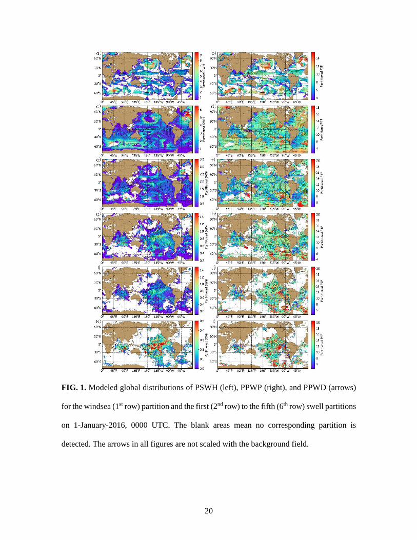
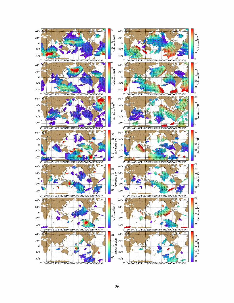
be guaranteed for the same partition label. For instance, Figure 1 shows the global

3

distributions of PSWH, PPWD, and PPWP for the windsea partition and the first five most

energetic swell partitions on 1-January-2016, 0000 UTC from a WW3 output field (the

data used here will be introduced in section 3). Discontinuity can be observed in all

partitions for all three parameters, especially in partitions with larger label numbers,

making it difficult to observe the features of wave fields in most of these plots. Meanwhile,

the continuity of these parameters might skip from one partition to another, even between

a windsea partition and a swell partition. This figure is similar to Figure 2 in Delpey et al.

(2010) where a similar problem is discussed. The time series for any given partition at any

given location may also exhibit discontinuity within the same partition label (not shown

here). To generate a coherent wave event, some spatial and temporal tracking algorithms

are developed to track waves that originate from the same meteorological event. There are

two types of wave event tracking methods. One involves back-tracking the wave based on

the linear dispersion relation to test whether a group of wave parameters corresponds to a

unique (e.g., Aarnes and Krogstad, 2001) or known (e.g., Delpey et al., 2010) source. This

type of method works only for “old” swells which have propagated into “far fields” while

it cannot apply to windseas and young swells because the non-linear wave-wave interaction

is not usually taken into consideration in backing-tracking. The other type of tracking

algorithm makes use of wave parameter continuity in space-time neighboring grid points

for the same wave event (e.g., Voorrips et al., 1997; Hanson and Phillips, 2001; Devaliere

et al., 2009). The temporal tracking scheme proposed by Hanson and Phillips (2001) is

widely used to track time series of wave events (e.g., Jiang et al., 2016), and a spatial

tracking scheme is proposed by Devaliere et al. (2009) using a “spiral searching” algorithm.

4

Both the temporal and spatial tracking schemes are implemented in WW3 (Van der

Westhuysen et al., 2013; The WAVEWATCH III® Development Group, 2016).

Temporal tracking is conducted on a one-dimensional time series so that the search

strategy can be simply searching from one time point to the next, but spatial tracking of

wave events is conducted on a two-dimensional “map” so that different search algorithms

can be applied. Devaliere et al. (2009) develop a “spiral search” algorithm to merge wave

components into wave events. However, this algorithm is designed for rectangular grids

and is not directly applicable to unstructured grids (Devaliere et al., 2009; Van der

Westhuysen et al., 2013). In addition, the “spiral search” algorithm is often influenced by

the land effect, which reduces the efficiency. The aim of this study is to present an

algorithm for spatially tracking wave events that is applicable for both structured and

unstructured grids.

2. Breadth-first tracking of wave field

The process of wave event spatial tracking involves searching for the wave

components in all neighboring grid points with a small variation of wave parameter, which

can be regarded as a process of graph traversing. A widely used traversing algorithm,

breadth-first search (BFS), should therefore be a good tool for this task. BFS starts at any

grid point in the wave field and explores all the neighboring grid points prior to moving on

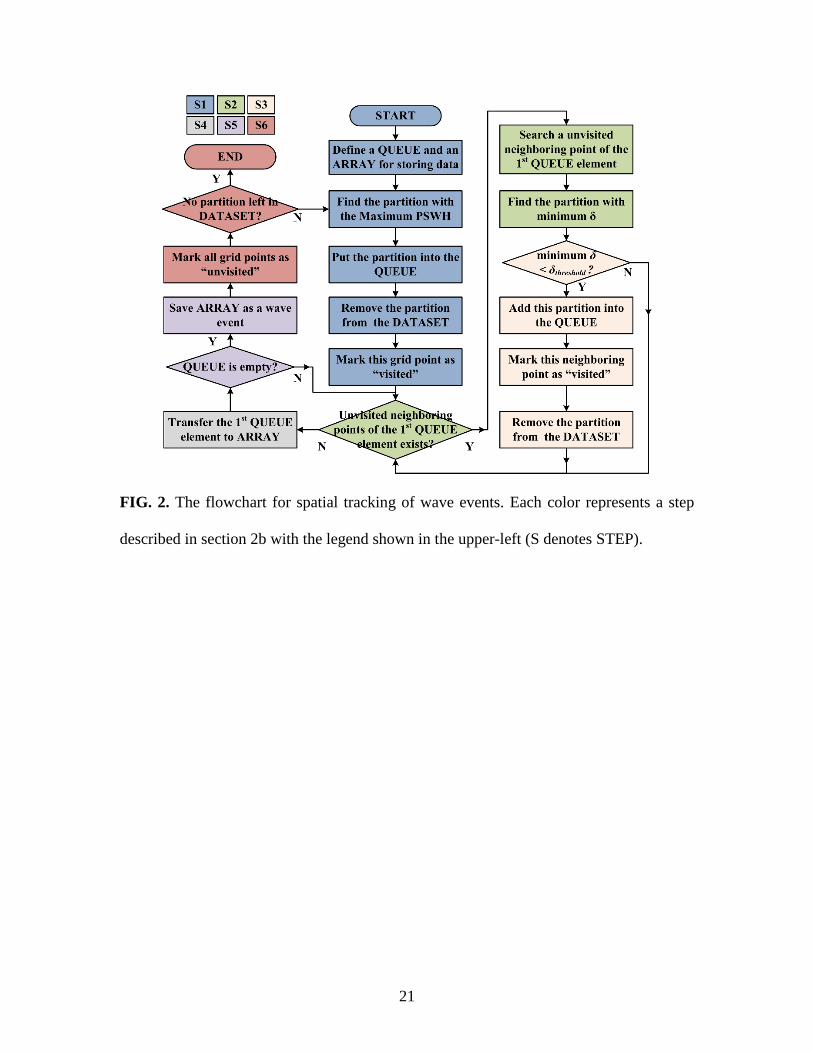
to one of them. Based on this algorithm, wave events are spatially tracked as shown in the

flowchart in Figure 2 and described below:

(1) Start the search from any partition at any grid point. Put this partition into a queue

(a first-in-first-out array), remove it from the original dataset, and mark this grid point as

5

“visited”. Here, the starting grid point and partition are specified as the grid point and

partition with the global maximum PSWH.

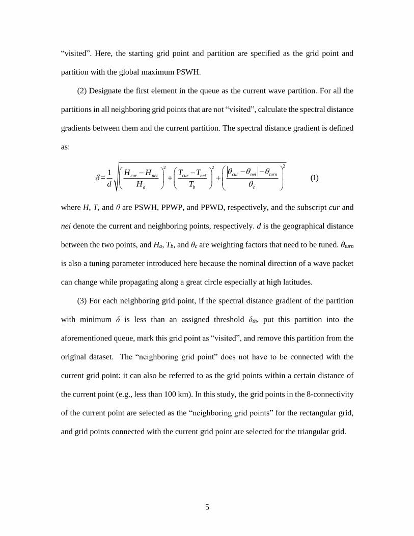
(2) Designate the first element in the queue as the current wave partition. For all the

partitions in all neighboring grid points that are not “visited”, calculate the spectral distance

gradients between them and the current partition. The spectral distance gradient is defined

as:

22 2

1= (1)

cur nei turncur nei cur nei

a b c

H H T T

d H T

where H, T, and θ are PSWH, PPWP, and PPWD, respectively, and the subscript cur and

nei denote the current and neighboring points, respectively. d is the geographical distance

between the two points, and Ha, Tb, and θc are weighting factors that need to be tuned. θturn

is also a tuning parameter introduced here because the nominal direction of a wave packet

can change while propagating along a great circle especially at high latitudes.

(3) For each neighboring grid point, if the spectral distance gradient of the partition

with minimum δ is less than an assigned threshold δth, put this partition into the

aforementioned queue, mark this grid point as “visited”, and remove this partition from the

original dataset. The “neighboring grid point” does not have to be connected with the

current grid point: it can also be referred to as the grid points within a certain distance of

the current point (e.g., less than 100 km). In this study, the grid points in the 8-connectivity

of the current point are selected as the “neighboring grid points” for the rectangular grid,

and grid points connected with the current grid point are selected for the triangular grid.

6

(4) When no partition meets the requirement of δ in any neighboring grid points of

the current partition, the current wave partition is transferred to another array that stores

the tracking results (the current wave partition is also removed from the queue).

(5) Repeat steps (2)-(4) until all the wave partitions in the queue are transferred to the

array storing the results. This result array then corresponds to a tracked wave event.

(6) Mark all grid points as “unvisited”, and then repeat from step (1) to track other

wave events until all the wave partitions are removed from the original dataset.

According to Equation 1, a small spectral distance gradient means that the PSWH,

PPWP, and PPWD are geographically changing slowly. It is noted that there is no

consensus on the definition of the spectral distance in Equation 1 (e.g., Hanson and Phillips,

2001, Delpey et al., 2009; Husson, 2012). Here, a form similar to the one given by Hanson

and Phillips (2001) is selected, but other definitions should also work. The values of the

tuning parameters, Ha, Tb, θc, and θturn, as well as the assigned threshold δth, are shown in

Table 1. During the tuning process, the value of Tb is set to 1 s, and the other parameters

are obtained through an iterative trial process. These values are with only one significant

digit because changing these values slightly have a very small impact on the tracking

results. The value of θturn is set to be proportional to the square of latitude because the

nominal direction change along a great circle is larger at high latitudes. The value of δth is

also regarded as being proportional to Hcur because newly generated waves usually have

both larger wave heights and larger gradient of wave parameters.

3. Test and improvement

Since the search process needs to compare only the wave parameters in neighboring

grid points, the tracking method presented in the above section should be applicable to any

7

partitioned NWM output in any type of grid, no matter whether it is structured or

unstructured. Because WW3 can provide standard output for partitioned wave information

in NetCDF format with one windsea system and up to five swell systems, the Integrated

Ocean Waves for Geophysical and other Applications (IOWAGA) dataset (Rascle and

Ardhuin, 2013), which is a hindcast dataset of WW3, is employed in this study to test the

algorithm. IOWAGA is an open-access dataset which contains the global information of

partitioned SWH, PWP, and PWD with a relatively high spatial-temporal resolution of

0.5°×0.5°×3h. This dataset is selected here for two primary reasons: (1) The data is

available for free from the FTP server of IFREMER where detailed information can also

be found. (2) This dataset shows good agreement with observations from buoys and

altimeters (e.g., Ardhuin et al., 2010) and is selected in some other studies of swell event

tracking (e.g., Delpey et al., 2010; Jiang et al., 2016). Figure 1 displays the information

contained in this dataset, and these data are also employed for the demonstration of the

tracking results. The dataset is organized in a structured grid. To test the performance of

the tracking method in an unstructured grid, the data is interpolated into a global triangular

grid generated by Gridgen software using the nearest neighbor approach. Other

interpolation approaches, such as linear or Kriging interpolation, are not used here due to

the discontinuity of wave parameters in the same partition label, or to say, interpolation

approaches involving more than one grid point have to be implemented after the spatial

tracking of wave events. There is almost no difference between the results for the structured

and unstructured grids.

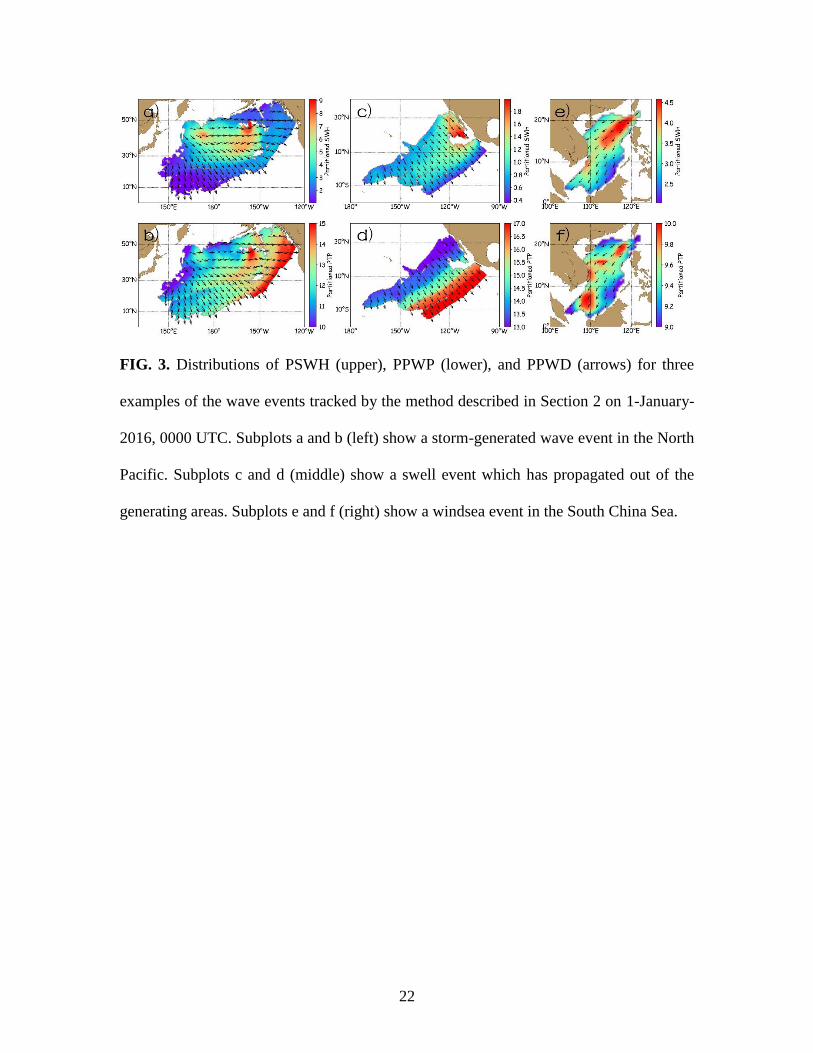
Three examples of the spatial tracking results are shown in Figure 3. The first example

is a storm-generated wave event in the North Pacific. A winter storm generates waves with

8

a PSWH of more than 6 m in the center of the wave field. The largest PPWP (~15s) is

observed in two locations: one corresponds to the largest PSWH, which is primarily due to

the strong wave-wave interaction in windseas, and the other is near the spatial boundary of

the wave event along the wave direction, which is primarily due to the frequency dispersion

of swells. Parts of this event should be regarded as windseas while parts of it should be

regarded as swells, and this event implies that there is no clear distinction between the two

types of wind-waves. The second example is a pure swell case which can be identified from

the rainbow-like pattern of PPWP: a clear PPWP gradient is observed along the

propagation direction of the wave field but the gradient is almost zero along the cross-

propagation direction. When waves propagate far away from their generating areas, the

spectra become narrow and the wave-wave interactions are negligible. The swells with

higher PPWPs travel faster than those with lower PPWPs because of the dispersion relation,

resulting in the rainbow-like period striping. The SWH distribution in the second case

shows clear anisotropy which is discussed in Delpey et al. (2010), and the highest wave

energy is found in the intermediate periods of the wave event. The third example is a typical

windsea event (as can be seen in Figure 1a and 1b) generated by the winter monsoon in the

South China Sea. Since the fetch is short in such a semi-enclosed sea, it is difficult for the

frequency dispersion to separate the energy with different periods or for the wave to reach

a fully-developed state. Therefore, the distribution of PPWP is relatively homogeneous in

this event and only varies in the range of 9~10 s.

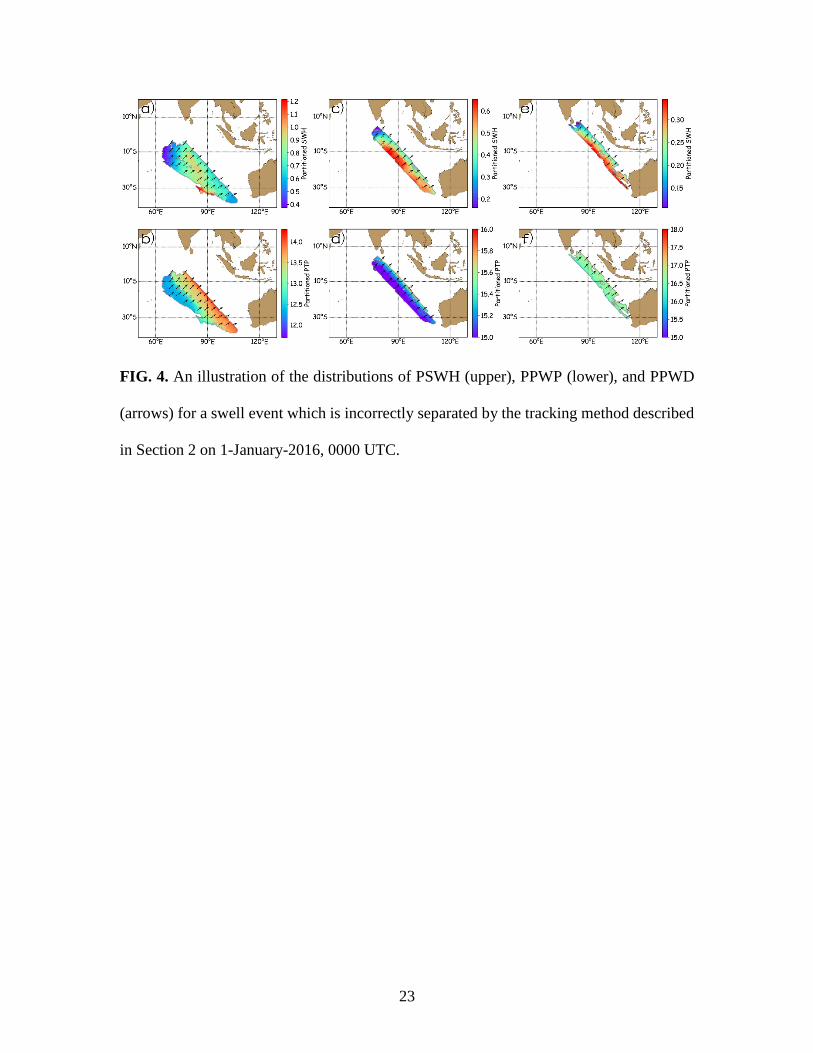
Using this method, tens of such wave events are spatially tracked at the same time.

During the test, however, it is found that the same swell event might be wrongly separated

into several fields with different PPWPs and PSWHs due to the garden sprinkler effect

9

(GSE) of frequencies along swell propagation directions (Tolman, 2002). An example is

shown in Figure 4 where the spatial boundaries of “three” wave events seem to be in good

agreement with each other. The PPWDs of them are generally the same, and the

PSWHs/PPWPs of them decrease/increase gradually along the wave propagation direction.

Clearly, they belong to the same swell event. Although the GSE can be greatly alleviated

by some numerical schemes (e.g., Tolman, 2002), it is still well-defined in the model output

especially for swells in the far field where the spectra are very narrow. In this case, the

GSE leads to a PPWP difference of ~0.5 s between adjacent grids. This difference

corresponds to a spectral distance gradient of 10-2 order of magnitude, which is much larger

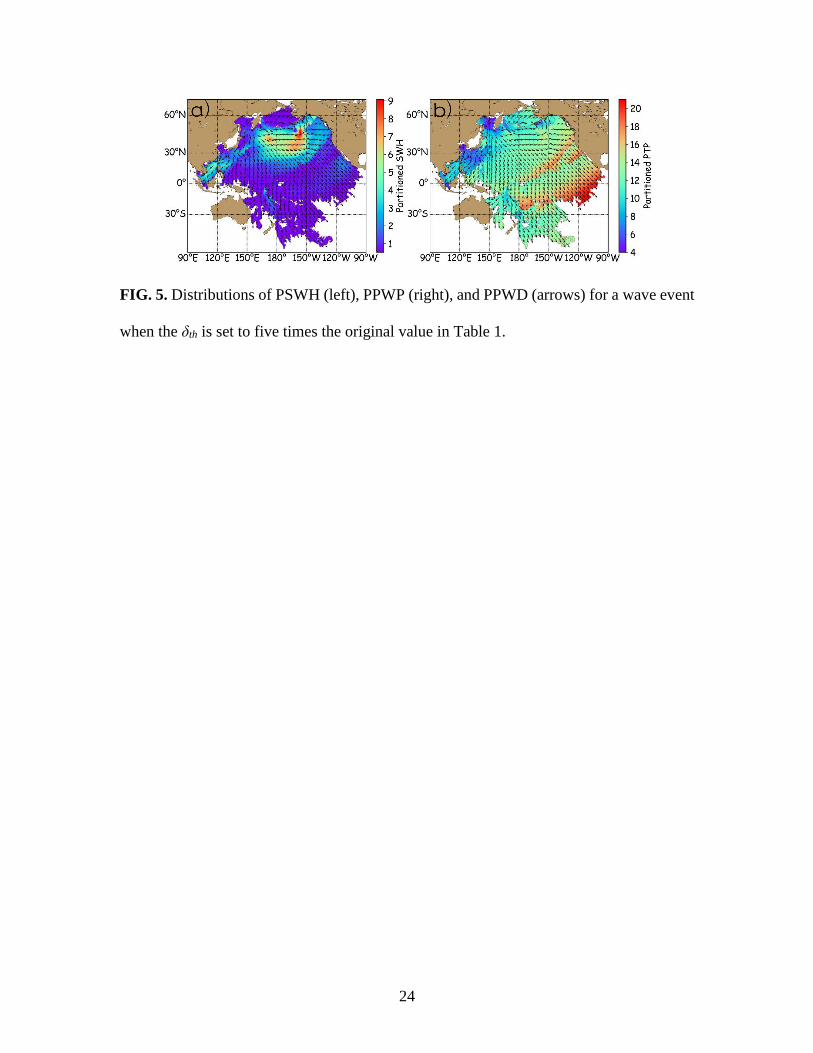
than the δth. Simply increasing the value of δth can partially solve the problem, but it will

also lead to other problems as shown in Figure 5 where the δth is set to 5×10-3 + 5×10-3Hcur

km-1, five times the original value. For visual analysis, results like Figure 5 are acceptable

as the wave parameters in Figure 5 are already much more organized and continuous

compared to Figure 1. However, distinct discontinuity of wave parameters is observed

especially in the PPWP. For instance, the forerunners of some swell events come into

contact with the lower frequency components of some other swell events. Also, it is noted

that the three wave events in Figure 3 are regarded as the same event in Figure 5 when the

δth is enlarged.

To better separate different wave events while minimizing the impact of the GSE, a

corresponding procedure termed “event merging” is applied for the wave events of which

the boundaries are in good agreement. To determine whether two tracked events can be

merged, the following criteria are used:

10

(1) Overlap Test: If the spatial extents of the two wave events have significant overlap,

they will not be regarded as being from the same wave event. In this case, the threshold

grid number of overlap is set to 1‰ of the grid number of the wave event with the lower

grid number.

(2) Boundary Test: Extend the spatial extent of one of the two events for two grid

points (i.e., dilate the boundary of one of the events by two grid points from a graphics

point of view). If the extended spatial extent does not have significant overlap with the

spatial extent of the other event (i.e., the boundaries of two tracked wave events are

inconsistent), the two events cannot be merged. Here, this threshold grid number of overlap

is simply set to 10 which works well for the test dataset.

(3) Wave Parameter Test: If the spatial distance between the two points respectively

from two to-be-merged tracked wave events which are not filtered by the above two criteria

is within 150 km, they are referred to as a point pair. If the mean spectral distance gradient

of all point pairs is within a threshold δth2, the two tracked wave events will be merged.

Here, the value of δth2 is set to 4×10-3+2×10-4 Nov (in km-1) where Nov is the number of

overlapping grid points in the above Boundary Test (2). The idea of introducing Nov is that

the possibility of the two tracked wave results being from the same events will be larger if

their boundaries are in better agreement. This value works well for this dataset, and

changing it within ±20% has almost no influence on the results due to the first two criteria.

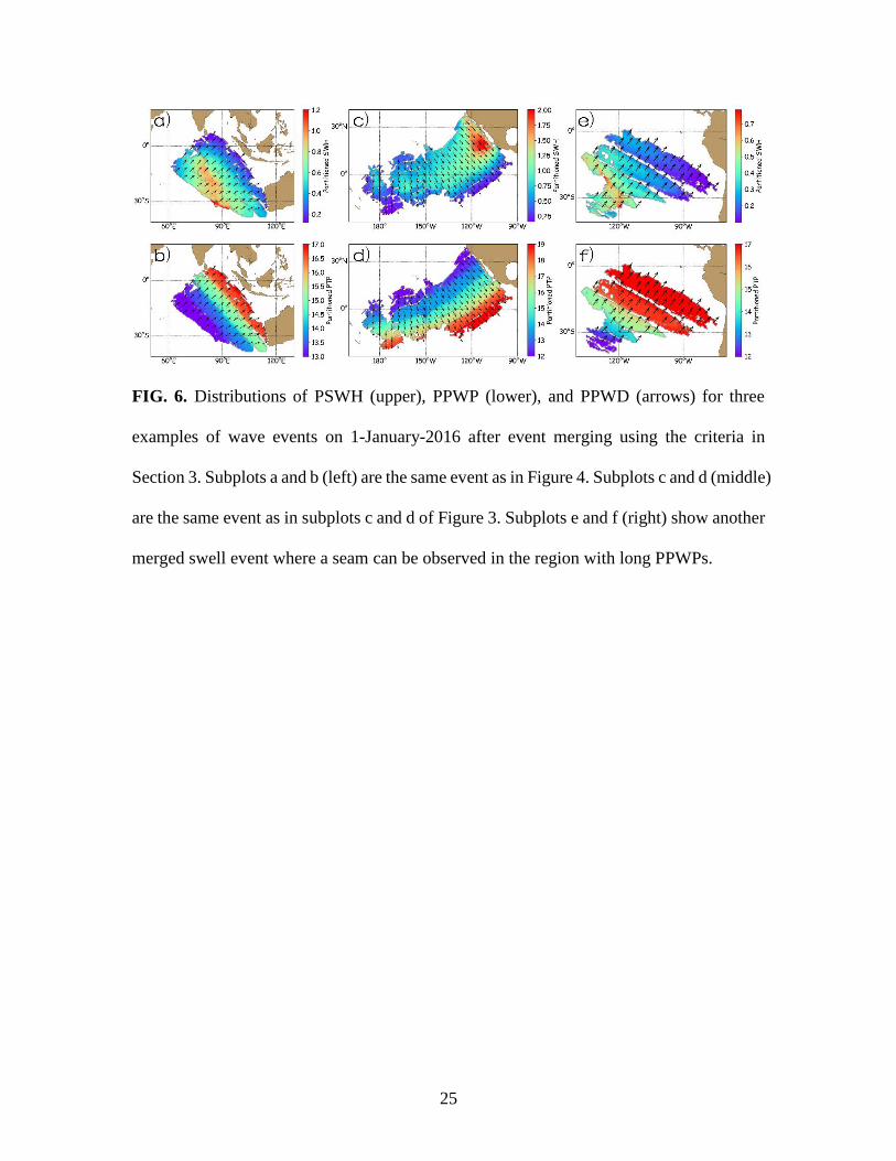
After merging, the three tracked results in Figure 4 are merged into one in Figures 6a

and 6b, showing that they are indeed the same event. Figures 6c and 6d show the same

event of the one in Figures 3c and 3d, but the spatial extent of the event appears to be larger

after merging the long-PPWP stripes, and some data gaps are filled (e.g., the region with

11

the maximum PSWH), showing the improvement of the tracking results using this merging

procedure. Figures 6e and 6f are also a case in which several tracked results are merged

into one wave event. In this case, a seam can be observed in the low-frequency (long-period)

part of the wave event. That is the reason why the spatial extent of one of the tracked events

is extended for two grid points instead of one in the above Boundary Test (2). The PSWH

near this seam is low (less than 0.2 m) so that the GSE might lead to lower wave energy in

this seam which might not be identified by the partitioning algorithm of Hanson and

Phillips (2001). These results all show that the GSE in the frequency direction has a

relatively large impact on swells with long periods in the far field. Although this effect

only has a very small impact on the simulation of overall SWHs due to the low energy

contribution of such partitions, it should be taken into account in tracking and modeling

the forerunners of ocean swells.

4. Summary and Discussion

Wave partitions in NWM output are usually organized without considering the

coherence of wave parameters in space, making it difficult to observe the features of wave

fields. In this study, an approach for spatially tracking coherent wave events using

partitioned NWM output is presented to solve this problem. This two-step method first

traverses the wave event using the continuity of wave parameters by BFS, then merges the

events of which the boundaries and the wave parameters on the boundaries are both in good

agreement. The BFS in the first step is an efficient traversal method which works for all

grid types. The second step is to reduce the impact of the GSE, which effectively improves

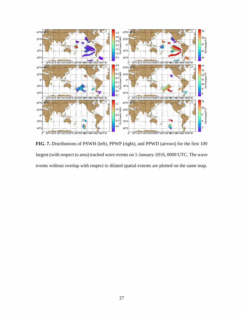
the tracking results. To have a better global view of the tested wave field, the first 100

largest (with respect to area) tracked wave events on 1-January-2016, 0000 UTC are shown

12

in Figure 7. The wave events without overlap with respect to the dilated spatial extents are

plotted on the same map. Although more than six maps are used to display the information

of the wave field (Figure 1 only uses six maps), the wave field features are much more

clearly-observed and more coherent in Figure 7 than those in Figure 1.

Although the results seem to be nice for some events, there are still two shortcomings

in this approach that the author fails to overcome at this stage. On the one hand, not all the

wave partitions are assigned to a wave event and the spatial extents of some tracked events

are small (only a few grid points, as shown in Figure 7). This is largely due to the error of

spectral partitioning algorithm itself. It is noted that the WW3 retains at most six partitions

at a given location, but sometimes more than six partitions can coexist. In addition, the

watershed-algorithm-based partitioning scheme (e.g., Hanson and Phillips, 2001) is a

purely morphological method that does not consider wave dynamics. When the energy

peak of a partition becomes smaller than the tail of a nearby partition, it might be

overwhelmed by the nearby partition, and the watershed-algorithm-based partitioning

scheme cannot identify it (Ailliot et al., 2013). Both of these might lead to discontinuity of

partitioned wave parameters in neighboring grid points and interrupt the procedure of wave

event tracking. On the other hand, only a single partition can be tracked at a given location,

because only the partition with the minimum spectral distance gradient at that point can be

included in the wave event according to this tracking method. However, this is not always

the case because the complicated space-time structure of the wind field might sometimes

lead to more than one partitions at the same location for the same event. Removing the step

of marking grid points as “visited” and including all the partitions with δ less than δth, rather

than only including the partition with minimum δ, can partially solve this problem.

13

Nevertheless, the author has not yet determined a way to visualize the results for the

condition that more than one partition is in the same grid point for the same wave event.

Despite these shortcomings, this spatial tracking method presented here can capture

the main features of partitioned wave fields from NWM output, and there are several

potential applications for it. As the visualization of the original NWM partitioned output

directly can only provide very limited information on the wave field due to the spatial

incoherence of identified partitions, the tracked results for wave events make it convenient

to have a quick view of the model output. The resulting spatially coherent wave fields can

be used to track the spatial-temporal evolution of wave events from windseas to swells,

which can be employed in the study of the space-time structure of wave fields (e.g., Delpey

et al., 2010). By comparing spatially-tracked model output with wave spectra

measurements from buoys, this approach can also be used to identify potential error sources

in wave modeling. Furthermore, this approach might serve as a potential tool for the data

assimilation of partitioned NWM output: if coherent evolution of wave events in the

NWMs can be obtained, wave data assimilation can be conducted at the “event” level by

assimilating in-situ measurements from buoys or remote sensing data from synthetic

aperture radars into the corresponding wave events. With the increasing attention being

paid to partitioned wave information in NWMs, such a spatial tracking approach could

contribute to both the scientific community and the marine industries.

Acknowledgments

The IOWAGA data are downloaded from IFREMER ftp (ftp.ifremer.fr).

REFERENCES

14

Aarnes, J. E, and H. E. Krogstad, 2001: Partitioning sequences for the dissection of

directional ocean wave spectra: A review. Tech. Rep., SINTEF Appl. Math., Oslo.

Ailliot, P., C. Maisondieu, and V. Monbet, 2013: Dynamical partitioning of directional

ocean wave spectra. Probabilist. Eng. Mech., 33, 95-102.

Ardhuin, F., et al., 2010: Semi-empirical dissipation source functions for wind-wave

models: Part I, Definition, calibration and validation. J. Phys. Oceanogr., 40, 1917-

1941.

Bidlot, J., 2016: Ocean wave model output parameters. [Available at

https://confluence.ecmwf.int/download/attachments/59774192/wave_parameters.pdf?

version=1&modificationDate=1470841648343&api=v2]

Collard, F., F. Ardhuin, and B. Chapron, 2009: Monitoring and analysis of ocean swell

fields from space: New methods for routine observations. J. Geophys. Res., 114,

doi:10.1029/2008JC005215.

Delpey, M. T., F. Ardhuin, F. Collard, and B. Chapron, 2010: Space-time structure of long

ocean swell fields. J. Geophys. Res., 115, doi:10.1029/2009JC005885.

Devaliere, E.-M., J. L. Hanson and R. Luettich, 2009: Spatial tracking of numerical wave

model output using a spiral tracking search algorithm, World Congress Comput. Sci.

Inf. Eng., Los Angeles, CA, 2, 404–408.

Gerling, T. W., 1992: Partitioning sequences and arrays of directional ocean wave spectra

into component wave systems. J. Atmos. Oceanic Technol., 9, 444-458.

Hanson, J. L., and O. M. Phillips, 2001: Automated analysis of ocean surface directional

wave spectra. J. Atmos. Oceanic Technol., 18, 277-293.

15

Husson, R., 2012: Development and validation of a global observation-based swell model

using wave mode operating Synthetic Aperture Radar, Ph.D. thesis, Dep. of Earth Sci.,

Univ. of Bretagne occidentale, Brest, France. (Available at http://tinyurl.com/kzm434f ).

Jiang, H., A. Babanin, and G. Chen, 2016: Event-Based Validation of Swell Arrival Time.

J. Phys. Oceanogr., 46, 3563-3569.

Jiang, H., A. Mouche, H. Wang, A. Babanin, B. Chapron, and G. Chen, 2017: Limitation

of SAR Quasi-Linear Inversion Data on Swell Climate: An Example of Global Crossing

Swells. Remote Sens., 9, doi:10.3390/rs9020107.

Portilla, J., F. J. Ocampo-Torres, and J. Monbaliu, 2009: Spectral Partitioning and

Identification of Wind Sea and Swell. J. Atmos. Oceanic Technol. 26, 107-122.

Rascle, N., and F. Ardhuin, 2013: A global wave parameter database for geophysical

applications. Part 2: Model validation with improved source term parameterization.

Ocean Modell., 70, 174-188.

The WAVEWATCH III® Development Group, 2016: User manual and system

documentation of WAVEWATCH III® version 5.16, Tech. Note,

NOAA/NWS/NCEP/MMAB, College Park, MD, USA. [Available at

http://polar.ncep.noaa.gov/waves/wavewatch/manual.v5.16.pdf]

Tolman, H. L., 2002: Alleviating the garden sprinkler effect in wind wave models. Ocean

Modell., 4, 269-289.

Tracy, B., E.-M. Devaliere, T. Nicolini, H. L. Tolman, and J. L. Hanson, 2007: Wind sea

and swell delineation for numerical wave modeling. Proc. 10th Int. Workshop on Wave

Hindcasting and Forecasting, Paper P12.

16

Van der Westhuysen, A., 2013: Spatial and Temporal Tracking of Ocean Wave Systems,

Mar. Model. and Anal. Branch, NOAA/NWS/NCEP/EMC. [Available at

http://polar.ncep.noaa.gov/waves/workshop/pdfs/wwws_2013_wave_tracking.pdf]

Voorrips, A. C., V. K. Makin, and S. Hasselmann, 1997: Assimilation of wave spectra from

pitch‐and‐roll buoys in a North Sea wave model. J. Geophys. Res., 102, 5829–5849

17

Figure & Table Captions

Table 1. The values of the tuning parameters.

FIG. 1. Modeled global distributions of PSWH (left), PPWP (right), and PPWD (arrows)

for the windsea (1st row) partition and the first (2nd row) to the fifth (6th row) swell partitions

on 1-January-2016, 0000 UTC. The blank areas mean no corresponding partition is

detected. The arrows in all figures are not scaled with the background field.

FIG. 2. The flowchart for spatial tracking of wave events. Each color represents a step

described in section 2b with the legend shown in the upper-left (S denotes STEP).

FIG. 3. Distributions of PSWH (upper), PPWP (lower), and PPWD (arrows) for three

examples of the wave events tracked by the method described in Section 2 on 1-January-

2016, 0000 UTC. Subplots a and b (left) show a storm-generated wave event in the North

Pacific. Subplots c and d (middle) show a swell event which has propagated out of the

generating areas. Subplots e and f (right) show a windsea event in the South China Sea.

FIG. 4. An illustration of the distributions of PSWH (upper), PPWP (lower), and PPWD

(arrows) for a swell event which is incorrectly separated by the tracking method described

in Section 2 on 1-January-2016, 0000 UTC.

18

FIG. 5. Distributions of PSWH (left), PPWP (right), and PPWD (arrows) for a wave event

when the δth is set to five times the original value in Table 1.

FIG. 6. Distributions of PSWH (upper), PPWP (lower), and PPWD (arrows) for three

examples of wave events on 1-January-2016 after event merging using the criteria in

Section 3. Subplots a and b (left) are the same event as in Figure 4. Subplots c and d (middle)

are the same event as in subplots c and d of Figure 3. Subplots e and f (right) show another

merged swell event where a seam can be observed in the region with long PPWPs.

FIG. 7. Distributions of PSWH (left), PPWP (right), and PPWD (arrows) for the first 100

largest (with respect to area) tracked wave events on 1-January-2016, 0000 UTC. The wave

events without overlap with respect to dilated spatial extents are plotted on the same map.

19

Table 1. The values of the tuning parameters.

Parameters Values (Unit)

Ha 2 (m)

Tb 1 (s)

θc 10 (°)

θturn Max [5×sin2(φ), |θcur-θnei|] (°) *

δth 10-3 + 10-3Hcur (km-1)

* φ is the latitude of the current grid point.

20

FIG. 1. Modeled global distributions of PSWH (left), PPWP (right), and PPWD (arrows)

for the windsea (1st row) partition and the first (2nd row) to the fifth (6th row) swell partitions

on 1-January-2016, 0000 UTC. The blank areas mean no corresponding partition is

detected. The arrows in all figures are not scaled with the background field.

21

FIG. 2. The flowchart for spatial tracking of wave events. Each color represents a step

described in section 2b with the legend shown in the upper-left (S denotes STEP).

22

FIG. 3. Distributions of PSWH (upper), PPWP (lower), and PPWD (arrows) for three

examples of the wave events tracked by the method described in Section 2 on 1-January-

2016, 0000 UTC. Subplots a and b (left) show a storm-generated wave event in the North

Pacific. Subplots c and d (middle) show a swell event which has propagated out of the

generating areas. Subplots e and f (right) show a windsea event in the South China Sea.

23

FIG. 4. An illustration of the distributions of PSWH (upper), PPWP (lower), and PPWD

(arrows) for a swell event which is incorrectly separated by the tracking method described

in Section 2 on 1-January-2016, 0000 UTC.

24

FIG. 5. Distributions of PSWH (left), PPWP (right), and PPWD (arrows) for a wave event

when the δth is set to five times the original value in Table 1.

25

FIG. 6. Distributions of PSWH (upper), PPWP (lower), and PPWD (arrows) for three

examples of wave events on 1-January-2016 after event merging using the criteria in

Section 3. Subplots a and b (left) are the same event as in Figure 4. Subplots c and d (middle)

are the same event as in subplots c and d of Figure 3. Subplots e and f (right) show another

merged swell event where a seam can be observed in the region with long PPWPs.

26

27

FIG. 7. Distributions of PSWH (left), PPWP (right), and PPWD (arrows) for the first 100

largest (with respect to area) tracked wave events on 1-January-2016, 0000 UTC. The wave

events without overlap with respect to dilated spatial extents are plotted on the same map.