CLOSURE METHOD FOR SPATIALLY AVERAGED DYNAMICS OF

PARTICLE CHAINS

ALEXANDER PANCHENKO, LYUDMYLA L. BARANNYK, AND ROBERT P. GILBERT

Abstract. We study the closure problem for continuum balance equations that model mesoscale dynamics

of large ODE systems. The underlying microscale model consists of classical Newton equations of particle

dynamics. As a mesoscale model we use the balance equations for spatial averages obtained earlier by anumber of authors: Murdoch and Bedeaux, Hardy, Noll and others. The momentum balance equation con-

tains a flux (stress), which is given by an exact function of particle positions and velocities. We propose amethod for approximating this function by a sequence of operators applied to average density and momen-

tum. The resulting approximate mesoscopic models are systems in closed form. The closed from property

allows one to work directly with the mesoscale equaitons without the need to calculate underlying particletrajectories, which is useful for modeling and simulation of large particle systems. The proposed closure

method utilizes the theory of ill-posed problems, in particular iterative regularization methods for solving

first order linear integral equations. The closed from approximations are obtained in two steps. First, weuse Landweber regularization to (approximately) reconstruct the interpolants of relevant microscale quanti-

tites from the average density and momentum. Second, these reconstructions are substituted into the exact

formulas for stress. The developed general theory is then applied to non-linear oscillator chains. We conducta detailed study of the simplest zero-order approximation, and show numerically that it works well as long

as fluctuations of velocity are nearly constant.

Key Words: FPU chain, particle chain, oscillator chain, upscaling, model reduction, dimension reduction,closure problem,

1. Introduction

In a series of papers, [1], [2], [3], [4], Murdoch and Bedeaux studied continuum mechanical balanceequations for mesoscopic space time averages of discrete systems. Earlier work of Irving and Kirkwood [14],Noll [16], and Hardy [13] on closely related topics should be also mentioned here. The fluxes in balanceequations (e. g. stress) are given by exact formulas as functions of particle positions and velocities. This isuseful for linking microscale dynamics with mesoscale phenomena. However, using these formulas requires acomplete knowledge of underlying particle dynamics. Since many particle systems of interest have enormoussize, direct simulation of particle trajectories may be intractable. Consequently, it makes sense to lookfor closed form approximations of fluxes in terms of other mesoscale quantities (e.g., average density andvelocity), rather than microscopic variables.

In this paper we address the above closure problem for spatially averaged mesoscale dynamics of largesize classical particle chains. The design of the method was influenced by the following considerations.

(1) The quantities of interest are space-time continuum averages, such as density, linear momentum,stress, energy and others. This choice of averages is natural because these quantities are experimen-tally measurable, and also because of their importance in coupled multiscale simulations involvingboth continuum and discrete models. In addition, by working directly with space-time averages in-stead of ensemble averages one can bypass a difficult problem of relating probabilistic and space-timeaverages.

(2) It is desirable to be able to predict behavior of averages on arbitrary time intervals, no matterhow short. This perspective comes from PDE problems, where observation time is often arbitraryand long time behavior is not of interest. When one tracks an ODE systems on an arbitrary timeinterval, transients may be all that is observed. Therefore, we do not use qualitative theory of ODEs,primarily concerned with describing long time features of dynamics. This significantly decreases therange of available tools. However, the closure problem for mesoscopic PDEs turned out to be a

2000 Mathematics Subject Classification. 82D25, 35B27, 35L75, 37Kxx, 70F10, 70Hxx, 74Q10, 82C21, 82C22.

1

arX

iv:1

010.

4832

v1 [

mat

h-ph

] 2

3 O

ct 2

010

question that can be still answered in a satisfactory way. The methods developed in this fashion canbe helpful in situations where long time features are not of interest: modeling transient and short-lived phenomena, working with metastable systems, and dealing with problems for which relaxationtimes can be hard to estimate.

(3) We consider particle systems with initial conditions that either known precisely, or ar least such thatthe possible initial positions and velocities are strongly restricted by available a priori information.This is in contrast to statistical mechanics, where uncertainty of initial conditions is a major problem.In this regard we note that our approach makes sense for discrete models of solid-fluid continuumsystems, where the smallest relevant length scale is still much larger than a typical intermoleculardistance. For other particle systems, our method can be used to run deterministic simulationsrepeatedly, in order to accumulate statistical information about the underlying probability density.

(4) Because of widespread use of computers in physical and engineering sciences, it is useful to developtheories tailored for computation, rather than ”paper and pencil” modeling. As far as the closureproblem is concerned, traditional phenomenological approach to formulating constitutive equationscan be subsumed by a more general problem of finding a computational closure method. In particular,a closure method can be realized as an iterative procedure where one inputs the values of the primaryvariables (e.g. density and velocity) computed at the previous moment of time, and the algorithmgenerates the flux (e.g. stress) at the next moment. Then primary variables are updated usingmesoscopic balance equations, and the process is repeated. In addition, focusing on computingone can obtain unconventional but useful continuum mechanical models. By replacing a simple,but possibly crude, Taylor series truncation with an algorithm we make it harder to obtain exactsolutions. Since such solutions are rarely available even for simple classical systems, (e.g. Navier-Stokes equations), this is not a serious drawback. On the positive side, computational closuregenerally contains an explicit (explicitly computable) link between micro- and mesoscale properties.

(5) An important potential application of closure is development of fast numerical methods for simulatingmeso-scopic dynamics of particle systems. Mesoscale solvers usually employ coarse meshes with meshsize much larger than a typical interparticle distance. Then the averages would be usually given bytheir coarse mesh values, while interpolants of microscale quantities are discretized on a fine scalemesh. Consequently, a closure method might consist of two generic blocks: (i) reconstruction onmesoscale mesh thereby a coarse approximations of fine scale quantities are obtained from averages;and (ii) interpolation of the obtained coarse scale discretizations to fine scale.

The closure algorithm developed in the paper is based on iterative regularization methods for solvingfirst kind integral equations. We observe that primary mesoscale averages are related to the interpolants ofmicroscale variables via a linear convolution operator. The kernel of this operator is the ”window function”used in [1] to generate averages. Such integral operators are usually compact. A compact operator may beinvertible, but the inverse operator is not continuous. Therefore, the problem of reconstructing microscalequantities from given averages is ill-posed. Such problems are well studied in the literature [12, 6, 9, 15, 18].A particular method used in the paper for inverting convolutions is Landweber iteration [5], [10]. It is knownthat if the error in the data tends to zero, the Landweber method produces successive approximationsconverging to the exact solution. For the merely bounded data error, convergence is replaced by a stoppingcriterion. This criterion provides the optimal number of iterations needed to approximate the solution withthe accuracy proportional to the error in the data. As a consequence, our method has desirable feature: onecan improve the approximation quality at the price of increasing the algorithm complexity. This means thatpredictive capability of the method can be regulated depending on available computing power.

The paper is organized as follows. In Section 2 we describe a general multi-dimensional microscopicmodel. The equations of motion are classical Newton equations. We limit ourselves to the case of shortrange interaction forces that may be either conservative or dissipative. The scaling of particle masses andforces reflects a continuum mechanical perspective, that is a family of particle systems of increasing sizeshould represent a hypothetical continuum material. As N → ∞, the total mass of the system shouldremain fixed, and the total particle energy should be either fixed, or at least bounded independent of N .Next, we recall the main points of averaging theory of Murdoch-Bedeaux and provide mesoscopic balanceequations and exact formulas for the stress from [4]. In Section 3 we develop integral approximations ofaverages, and describe the use of Landweber iterative regularization for approximate reconstruction. Section

2

4 contains the formulation of the scaled ODE equations of the so-called Fermi-Pasta-Ulam (FPU) chains.In Section 5 we derive closed form mesoscopic continuum equations of chain dynamics. The complexity ofthese continuum models increases with the order n of the iterative deconvolution approximation. Section 6is devoted to the detailed study of the simplest closed model with n = 0, which we call zero-order closure.Essentially, zero-order closure means that the microscopic quantities are replaced by their averages. Suchan approximation can work well only for systems with small fluctuations. To quantify fluctuation size weintroduce upscaling temperature and the related notion of quasi-isothermal dynamics. For such dynamics, weshow how to interpolate averages given by mesoscopic mesh values, in order to initialize approximate particlepositions and velocities. The interpolation procedure is problem-specific: it conserves microscopic energyand preserves quasi-isothermal nature of the dynamics. Section 7 contains the results of computational tests.Here we apply our zero-closure algorithm to a Hamiltonian chain with the finite range repulsive potential U ,decreasing as a power of distance. The results show good agreement of zero-order approximations with theexact stress produced by direct simulations with 10000-80000 particles, provided the initial conditions havesmall fluctuations. In our example, the initial conditions are such that the upscaling temperature is nearlyzero during the observation time. We also demonstrate that increasing fluctuations of initial velocities leadsto a considerable increase in the approximation error, indicating that higher order closure algorithms shouldbe used instead of zero-order closure. Applicability of the zero-order closure is further discussed in Section8. Finally, conclusions are provided in Section 9.

2. Microscale equations and mesoscale spatial averages

2.1. Scaled ODE problems. The starting point is the microscale ODE problem. In this paper we shallwork with classical Newton equations of point particle dynamics. The same equations may arise as dis-cretization of the momentum balance equation for continuum systems. Consider a system containing N 1identical particles, denoted by Pi. The mass of each particle is M

N , where M is the total mass of the system.

Suppose that during the observation time T , Pi remain inside a bounded domain Ω in Rd, where d is thephysical space dimension, usually 1, 2 or 3. The positions qi(t) and velocities vi(t) of particles satisfy asystem of ODEs

qi = vi,(2.1)

M

Nvi = f i + f

(ext)i ,(2.2)

subject to the initial conditions

(2.3) qi(0) = xi, vi(0) = v0i .

Here f(ext)i denotes external forces, such as gravity and confining forces. The interparticle forces f i =

∑j f ij ,

where f ij are pair interaction forces which depend on the relative positions and velocities of the respectiveparticles.

We are interested in investigating asymptotic behavior of the system as N → ∞. Thus it is convenientto introduce a small parameter

(2.4) ε = N−1/d,

characterzing a typical distance between neighboring particles. As ε approaches zero, the number of particlesgoes to infinity, and the distances between neighbors shrink. Consequently, the forces in (2.2) should beproperly scaled. The guiding principle for scaling is to make the energy of the system bounded independentof N , as N →∞. In addition, the energy of the initial conditions should be bounded uniformly in N .

As an example of scaling, consider forces generated by a finite range potential U and assume that eachparticle interacts with no more than a fixed number of neighbors (this is the case, e.g., for particle chainswith nearest neighbor interaction, where a particle always interacts with two neighbors). The fixed numberof interacting neighbors implies that there are about N interacting pairs. Assuming also that the systemis sufficiently dense, and variations of particle concentrations are not large, we can suppose that a typicaldistance between interacting particles is on the order N−1/dL = εL. The resulting scaling

(2.5) f ij = − 1

εN∇xU

(qj − qk

ε

)3

makes the potential energy of an isolated system bounded independent of N . Kinetic energy will be undercontrol provided the total energy of the initial conditions is bounded independent of N . If exterior forcesare present, they should be scaled as well.Remark. Superficially, the system (2.1), (2.2) looks similar to the parameter-dependent ODE systems studiedin numerous works on ODE time homogenization (see e g. [17] and references therein). In the problemunder study, ε depends on the system dimension N , while in the works on time-homogenization and ODEperturbation theory, the system size is usually fixed as ε→ 0.

2.2. Length scales. We introduce the following length scales:- macroscopic length scale L = diam(Ω);- microscopic length scale εL;- mesoscopic length scale ηL,where 0 < η < 1 is a parameter that characterizes spatial mesoscale resolution. This parameter is chosenbased on the desired accuracy, the computational cost requirements, available information about initialconditions and behavior of ODE trajectories etc.

The computational domain Ω is subdivided into mesoscopic cells Cβ , β = 1, 2, . . . , B, with the side lengthon the order of ηL. The centers xβ of Cβ are the nodes of the meso-mesh. The number of unknowns in themesoscopic system will be on the order of B. For computational efficiency, one should have B N . Thisdoes not mean that η is close to one. In fact, it makes sense to keep η as small as possible in order to havean additional asymptotic control over the system behavior. Decreasing η will in general make computationsmore expensive.

2.3. Averages and their evolution. To define averages we first select a fast decreasing window functionψ satisfying

∫ψ(x)dx = 1. There are many possible choices of the window function. In the paper we assume,

unless otherwise indicated, that ψ is a compactly supported, differentiable on the interior of its support, andnon-negative. Next, define

ψη(x) = η−dψ

(x

η

).

Once the window function is chosen, we can evaluate the averages of various continuum mechanicalvariables, following [1], [4]. The mesoscopic average density and momentum are given by

(2.6) ρη(t,x) =M

N

N∑i=1

ψη(x− qi(t)),

(2.7) ρηvη(t,x) =M

N

∑vi(t)ψη(x− qi(t)).

The meaning of the above definitions becomes clear if one considers ψ = (cd)−1χ(x), where χ is a charac-

teristic function of the unit ball in Rd, and cd is the volume of the unit ball. Then

ρη =1

cdηdM

N

∑χ

(x− qi(t)

η

).

The sum in the right hand side gives the number of particles located within distance η of x at time t.Multiplying by M/N we get the total mass of these particles, and dividing by cdη

d (the volume of η-ball)gives the usual particle density.

Differentiating (2.6), (2.7) in t, and using the ODEs (2.1), (2.2) one can obtain [1] exact mesoscopic

balance equations for all primary variables. For example, for an isolated system with (f(ext)i = 0), mass

conservation and momentum balance equations take the form:

(2.8) ∂tρη + div(ρηvη) = 0,

(2.9) ∂t(ρηvη) + div (ρηvη ⊗ vη)− divT η = 0.

The stress T η = T η(c) + T η

(int) [4], where

(2.10) T η(c)(t,x) = −

∑mi(vi − vη(t,x, ))⊗ (vi − vη(x, t))ψ(x− qi)

4

is the convective stress, and

(2.11) T η(t,x)(int) =∑(i,j)

f ij ⊗ (qj − qi)

∫ 1

0

ψ(s(x− qj) + (1− s)(x− qi)

)ds

is the interaction stress. The summation in (2.11) is over all pairs of particles (i, j) that interact with eachother.

Discretizing balance equations on the mesoscopic mesh yields a discrete system of equations, called themeso-system, written for mesh values of ρηβ , (ρ

ηvη)β and T ηβ . The dimension of the meso-system is much

smaller than the dimension of the original ODE problem. However, at this stage we still have no compu-tational savings, since the meso-system is not closed. This means that mesoscopic fluxes such as (2.10),(2.11) are expressed as functions of the microscopic positions and velocities. To find these positions andvelocities, one has to solve the original microscale system (2.1), (2.2). To achieve computational savings weneed to replace exact fluxes with approximations that involve only mesoscale quantities. We refer to theprocedure of generating such approximations as a closure method. This closure-based approach has muchin common with continuum mechanics. The important difference is that the focus is on computing, ratherthan continuum mechanical style modeling of constitutive equations.

3. Closure via regularized deconvolutions

3.1. Outline. Our approach is based on a simple idea: the integral approximations of primary averages(such as density and velocity) are related to the corresponding microscopic quantities via convolution withthe kernel ψη. Therefore, given primary variables we can (approximately) recover the microscopic positionsand velocities by numerically inverting convolution operators. The results are inserted into equations forsecondary averages (or fluxes), such as stress in the momentum balance. This yields closed form balanceequations that can be simulated efficiently on the mesoscopic mesh.

3.2. Integral approximation of discrete averages. To exploit the special structure of primary averages,it is convenient to approximate sums such as

(3.1) gη =1

N

N∑j=1

g(vj , qj)ψη(x− qj)

by integrals. Since particle positions qj are not periodically spaced, (3.1) is not in general a Riemann sumfor gψη(x − ·). To interpret the sum correctly, we introduce interpolants q(t,X), v(t, q) of positions andvelocities, associated with the microscopic ODE system (2.1), (2.2). At t = 0 these interpolants satisfy

q(0,Xj) = q0j , v(0, q(0,Xj)) = v0

j ,

where Xj , j = 1, 2, . . . , N are points of ε-periodic rectangular lattice in Ω. At other times,

q(t,Xj) = qj(t), v(t, q(t,Xj)) = vj(t).

Then we can rewrite (3.1) as

(3.2) gη =1

|Ω|

N∑j=1

|Ω|Ng (v (t, q(t,Xj)) , q(t,Xj)ψη(x− q(t,Xj)),

where |Ω| denotes the volume (Lebesgue measure) of Ω. Eq. (3.2) is a Riemann sum generated by partitioningΩ into N cells of volume |Ω|/N centered at Xj . This yields

(3.3) gη =1

|Ω|

∫Ω

g (v(t, q(t,X)), q(t,X))ψη(x− q(t,X))dX,

up to discretization error. Now suppose that the map q(·,X) is invertible for each t, that is X = q−1(t, q).Changing the variables in the integral y = q(t,X) we obtain a generic integral approximation

(3.4) gη =1

|Ω|

∫Ω

g (v(t,y),y)ψη(x− y)J(t,y) dy,

5

where

(3.5) J = |det∇q−1|,up to discretization error.

3.3. Regularized deconvolutions. Define an operator Rη by

Rη[f ](x) =

∫ψη(x− y)f(y)dy.

To simplify exposition, suppose that Rη is injective. For example, a Gaussian ψη produces an injectiveoperator, which is not difficult to check using Fourier transform and uniqueness of analytic continuation. If Rηis injective, then there exists the single-valued inverse operator R−1

η , that we call the deconvolution operator.

Unfortunately, this operator is unbounded, since Rη is compact in L2(Ω). This is the underlying reasonfor the popular belief that averaging destroys the high-frequency information contained in the microscopicquantities. In fact, this information is still there (the inverse operator exists), but it is difficult to recoverin a stable manner, because of unboundedness. This does not make the situation hopeless, as has beenrecognized for some time. Reconstructing f from the knowledge of Rη[f ]) is a classical example of anunstable ill-posed problem (small perturbations of the right hand side may produce large perturbations ofthe solution). The exact nature of ill-posedness and methods of regularizing the problem are well investigatedboth analytically and numerically (see, e. g. [6, 9, 15, 18, 11, 12]). Accordingly, we interpret notation R−1

η

as a suitable regularized approximation of the exact operator. Many regularizing techniques are currentlyavailable: Tikhonov regularization, iterative methods, reproducing kernel methods, the maximum entropymethod, the dynamical system approach and others. It is very fortunate that this vast array of knowledge canbe used for the ODE model reduction. On the conceptual level, our approach makes it clear that instabilityassociated with ill-posedness is a fundamental difficulty in the process of closing the continuum mechanicalequations.

A family of Landweber iterative deconvolution methods [5], [10] seems to be particularly convenient inthe present context. In the simplest version, approximations gn to the solution of the operator equation

(3.6) Rη[g] = gη

are generated by the formula

(3.7) gn =

n∑k=0

(I −Rη)ngη, g0 = gη.

The number n of iterations plays the role of regularization parameter. In (3.7), I denotes the identityoperator.

The first three low-order approximations are

g0 = gη n = 0,(3.8)

g1 = gη + (I −Rη)[gη] n = 1,(3.9)

g2 = gη + (I −Rη)[gη] + (I −Rη)2[gη] n = 2.(3.10)

4. Microscale particle chain equations

In this section, the general method outlined above is detailed in the case of one-dimensional Hamiltonianchain of oscillators that consists of N identical particles with nearest neighbor interaction. The domain Ω isan interval (0, L). Particle positions, denoted by qj = qj(t), j = 1, . . . , N , satisfy

0 < q1 < q2 < . . . < qN < L

at all times, i.e. the particles cannot occupy the same position or jump over each other. Next, define a smallparameter

ε =1

N,

and microscale step size

(4.1) h =L

N.

6

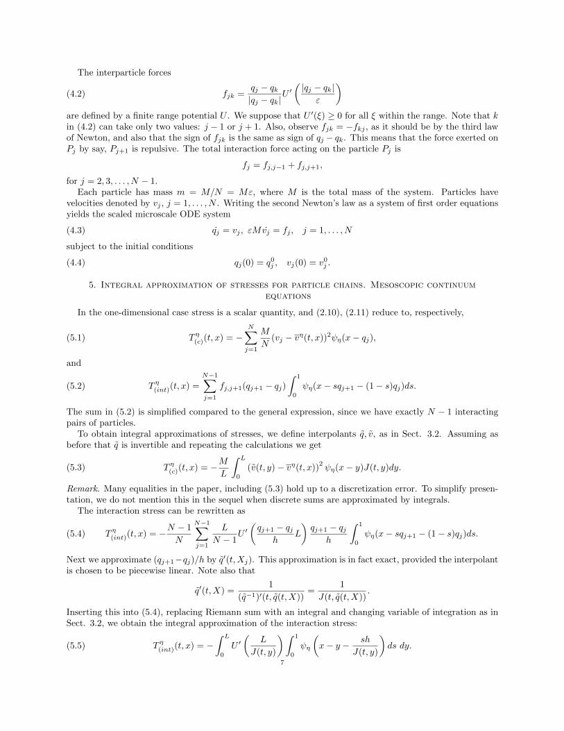
The interparticle forces

(4.2) fjk =qj − qk|qj − qk|

U ′(|qj − qk|

ε

)are defined by a finite range potential U . We suppose that U ′(ξ) ≥ 0 for all ξ within the range. Note that kin (4.2) can take only two values: j − 1 or j + 1. Also, observe fjk = −fkj , as it should be by the third lawof Newton, and also that the sign of fjk is the same as sign of qj − qk. This means that the force exerted onPj by say, Pj+1 is repulsive. The total interaction force acting on the particle Pj is

fj = fj,j−1 + fj,j+1,

for j = 2, 3, . . . , N − 1.Each particle has mass m = M/N = Mε, where M is the total mass of the system. Particles have

velocities denoted by vj , j = 1, . . . , N . Writing the second Newton’s law as a system of first order equationsyields the scaled microscale ODE system

(4.3) qj = vj , εMvj = fj , j = 1, . . . , N

subject to the initial conditions

(4.4) qj(0) = q0j , vj(0) = v0

j .

5. Integral approximation of stresses for particle chains. Mesoscopic continuumequations

In the one-dimensional case stress is a scalar quantity, and (2.10), (2.11) reduce to, respectively,

(5.1) T η(c)(t, x) = −N∑j=1

M

N(vj − vη(t, x))2ψη(x− qj),

and

(5.2) T η(int)(t, x) =

N−1∑j=1

fj,j+1(qj+1 − qj)∫ 1

0

ψη(x− sqj+1 − (1− s)qj)ds.

The sum in (5.2) is simplified compared to the general expression, since we have exactly N − 1 interactingpairs of particles.

To obtain integral approximations of stresses, we define interpolants q, v, as in Sect. 3.2. Assuming asbefore that q is invertible and repeating the calculations we get

(5.3) T η(c)(t, x) = −ML

∫ L

0

(v(t, y)− vη(t, x))2ψη(x− y)J(t, y)dy.

Remark. Many equalities in the paper, including (5.3) hold up to a discretization error. To simplify presen-tation, we do not mention this in the sequel when discrete sums are approximated by integrals.

The interaction stress can be rewritten as

(5.4) T η(int)(t, x) = −N − 1

N

N−1∑j=1

L

N − 1U ′(qj+1 − qj

hL

)qj+1 − qj

h

∫ 1

0

ψη(x− sqj+1 − (1− s)qj)ds.

Next we approximate (qj+1−qj)/h by q′(t,Xj). This approximation is in fact exact, provided the interpolantis chosen to be piecewise linear. Note also that

q′(t,X) =1

(q−1)′(t, q(t,X))=

1

J(t, q(t,X)).

Inserting this into (5.4), replacing Riemann sum with an integral and changing variable of integration as inSect. 3.2, we obtain the integral approximation of the interaction stress:

(5.5) T η(int)(t, x) = −∫ L

0

U ′(

L

J(t, y)

)∫ 1

0

ψη

(x− y − sh

J(t, y)

)ds dy.

7

Equations (5.3), (5.5) contain two microscale quantities: J and v. Approximating sums in the definitions ofthe primary averages (2.6), (2.7) by integrals we see that ρη and vη are obtained by applying the convolutionoperator Rη to, respectively J and Jv:

(5.6) ρη =M

LRη[J ], ρηvη =

M

LRη[Jv].

The discretization error in (5.6) can be made small by imposing suitable requirements on the microscopicinterpolants. Fortunately, the theory of ill-posed problems allows for errors in the right hand side of integralequations. The size of the error determines the choice of regularization parameter. In the present case,the error determines the number of iterations needed for the optimal reconstruction, according to so-calledstopping criteria. These criteria are available in the literature on ill-posed porblems (see e.g. [9]). Detailedinvestigation of these questions is left to future work.

Denote by R−1η,n the iterative Landweber regularizing operators

R−1η,n =

n∑k=0

(I −Rη)k.

Applying R−1η,n in (5.6) yields a sequence of approximations

(5.7) Jn =L

MR−1η,n[ρη], vn =

R−1η,n[ρηvη]

R−1η,n[ρη]

,

and a corresponding sequence of closed form mesoscopic continuum equations (written here for an isolatedsystem with zero exterior forces)

∂tρη + ∂x(ρηvη) = 0,(5.8)

∂t(ρηvη) + ∂x

(ρη(vη)2

)− ∂x(T η(c),n + T η(int),n) = 0,(5.9)

where T η(c),n, Tη(int),n are given by

(5.10) T η(c),n = −ML

∫ L

0

(vn(t, y)− vη(t, x))2ψη(x− y)Jn(t, y)dy,

(5.11) T η(int),n = −∫ L

0

U ′(

L

Jn(t, y)

)∫ 1

0

ψη

(x− y − sh

Jn(t, y)

)ds dy,

with Jn, vn given by (5.7).

6. Zero-order closure for particle chains

Let us consider zero-order approximations in detail. The mesoscopic mesh consists of points

xβ =

(β − 1

2

)ηL, β = 1, 2, . . . , B,

where B = 1/η, presumed to be an integer satisfying B N . Meso-cells are intervals Iβ of length

Lη = L/B = ηL,

centered at xβ .Suppose that the only primary variables of interest are density ρη and linear momentum ρηvη. These

variables will be computed by the mesoscale solver. For simplicity, suppose that the meso-solver is explicit intime. Then the average density and average velocity will be available at the previous moment of time. Ourtask is to design an update step for computing density and velocity at the next time moment. To construct aclosed form update step, we need to approximate stress T η in (2.9) in terms of ρη, ρηvη. From the knowledgeof ρη, ρηvη we can approximately recover J and Jv. The zero-order approximation (3.8) corresponds to

J(t, x) ≈ L

Mρη(t, x),(6.1)

J(t, x)v(t, x) ≈ L

Mρηvη(t, x).(6.2)

8

In other words, the microscale quantities are approximated by their averages. The corresponding closed formapproximations for stress are obtained by inserting (6.1), (6.2) into (5.10), (5.11):

(6.3) T η(c),0(t, x) = −∫ L

0

(vη(t, y)− vη(t, x))2ψη(x− y)ρη(t, y)dy,

(6.4) T η(int),0 = −∫ L

0

U ′(

M

ρη(t, y)

)∫ 1

0

ψη

(x− y − shM

Lρη(t, y)

)ds dy.

For computation, a numerical quadrature should be used. In this regard, note that all average quantities arecomputed on the mesoscale mesh, while the formulas (2.10), (2.11) are fine scale discretizations. Therefore,one might wonder if a straightforward mesoscale quadrature of (6.3), (6.4) is too crude. A better approachis to interpolate ρη, vη by prescribing approximate particle positions qj and velocities vj , j = 1, 2, . . . , N ,compatible with the given ρη, vη. Once this is done, (6.3), (6.4) can be discretized on a fine scale mesh withmesh nodes qj .

Interpolants cannot be unique. For zero-order closure, we are choosing positions and velocities that pro-duce the given average density and average velocity. Clearly, there are many different position-velocityconfigurations with the same averages. The choice made in the paper is motivated by the practical require-ment of achieving low operation count, as well as by certain expectations about the nature of dynamics.From the continuum mechanical point of view, if a system can be adequately modeled by balance equationsof mass and momentum, then it must have have a trivial energy balance. Most often this means that thedeformation is nearly isothermal. To mimic such isothermal dynamics we suppose that at each time step,there exists a positive number κ2 (it can be called ”upscaling temperature”) such that

(6.5)∑j∈Jβ

(vβj − vη(t, xβ))2ψη(xβ − qj) = κ2.

Here the summation is over all particles located in a meso-cell Iβ . The temperature κ2 is the same for allβ = 1, 2, . . . , B. We emphasize that the actual value of κ2 is not as important as the fact that its valueis the same for all meso-cells. This is because (6.5) would yield constant mesoscale mesh node values ofT η(c),0 As a result, the finite difference approximation of ∂xT

η(c),0 on the mesoscale mesh is identically zero.

We interpret this by saying that convective stress does not contribute to the mesoscopic dynamics in theisothermal case. Another observation is that κ need not be the same at different moments of time, so ourassumption is somewhat more flexible than the standard isothermal deformation approximation. Also, wenote that validity (6.5) depends on the choice of η. For bigger η, it is more likely that (6.5) holds for thesame underlying microscopic dynamics. Details on this are provided below in Section 6.2. Additionally,other features of the microscopic dynamics should be taken into account. Most importantly, interpolatedvelocities vj = vη(qj) must be such that the collection qj , vj , j = 1, 2, . . . , N conserves microscopic energy E :

(6.6) E =1

2

M

N

N∑j=1

(vj)2 + U(Q)

where U(Q) is the microscale potential energy corresponding to the positions qj .

6.1. Prescribing particle positions. The objective of this section is to assign approximate particle posi-

tions qj . We start by interpolating J . The simplest interpolant is piecewise-constant: J(t,x) ≈∑Bβ=1 J(t, xβ)χβ(x) =∑B

β=1LM ρη(t, xβ)χβ(x) where χβ is the characteristic function of the meso-cell Iβ . A simple choice of the

position map compatible with this interpolant is a piecewise linear map having the prescribed constant valueof J in each meso-cell. In practical terms, this means that in each meso-cell, particles are spaced at equalintervals from each other. The local interparticle spacing

(6.7) ∆β =M

ρη(t, xβ)N

is determined by the mesh value of the average density. To explain (6.7), note that the total mass of particlescontained in the meso-cell Iβ can be approximated by ρη(t, xβ)Lη. Dividing by the mass M/N of one particle,

9

we obtain an approximate number of particles inside Iβ :

nβ = ρη(t, xβ)LηN

M,

and thus ∆β = Lη/nβ . We emphasize that qj are chosen based only on the known mesh values of the densityρη, and that qj will be different from the actual particle positions qj .

Now we approximate the integral in (6.4) by its Riemann sum generated by the partition qj , j =1, 2, . . . , N:

T η(int),0 ≈ −N−1∑j=1

U ′ (N(qj+1 − qj)) (qj+1 − qj)∫ 1

0

ψη (x− sqj+1 − (1− s)qj) ds.(6.8)

6.2. Prescribing particle velocities. In order to approximate the convective stress in the fine scale dis-cretization of (6.3), we need to choose approximations vj of the true particle velocities vj . The choice of vjmust satisfy (6.6) and be compatible with the available average velocity at the mesoscale mesh nodes.

For each qj ∈ Iβ , we set

vj = vηβ + δvβj ,

where vηβ is the local average velocity, and δvβj is a perturbation to be defined.Next, we show that the energy-conserving collection of δvj velocity always exists, provided its upscaling

temperature is suitably prescribed. This prescription will be based only on the available mesoscale informa-tion. For definitiveness, in the rest of this section we suppose that ψη satisfies the following condition:

ψη(xβ − qj) > 0, if qj ∈ Iβ .(6.9)

To make the algebra simpler, we make another assumption: for each β = 1, 2, . . . , B,

(6.10)

N∑j=1

f(vj)ψη(xβ − qj) ≈∑j∈Jβ

f(vj)ψη(xβ − qj),

where f is either vj or (vj)2. The second summation is over all j such that qj ∈ Iβ . Assumption (6.10) holds

when ψη(xβ − y) is small outside of Iβ .Averaging of vj should produce the known average velocity vηβ . This yields an equation for δvj :

(6.11)M

N

∑j∈Jβ

vjψη(xβ − qj) = ρηβvηβ .

SinceM

N

∑j∈Jβ

vjψη(xβ − qj) = vηβM

N

∑j∈Jβ

ψη(xβ − qj) +M

N

∑j∈Jβ

δvβj ψη(xβ − qj)

= ρηβvηβ +

M

N

∑j∈Jβ

δvβj ψη(xβ − qj),

(6.11) holds provided

(6.12)M

N

∑j∈Jβ

δvβj ψη(xβ − qj) = 0.

Now we look for perturbations in the form

(6.13) δvβj =aβj

ψη(xβ − qj),

where the aβj are to be determined. Next, narrow down the choice of aβj by setting

(6.14) aβj = taβj ,

where aβj is either one or negative one. To satisfy (6.12) we need nβ to be even (one more point can be easily

inserted if the actual nβ is odd); in addition, the number of positive and negative aβj must be the same.10

To simplify further calculations, we write conservation of energy (6.6) in the form

(6.15)∑j∈Jβ

(δvβj )2 = Kβ ,

where Kβ are any numbers satisfying

(6.16) Kβ > 0,

B∑β=1

Kβ =2N

M

E − U(Q)− 1

2

M

N

B∑β=1

(vηβ)2nβ

.

Our goal now is to show that there is a choice of Kβ , κ2 and t such that δvβj defined by (6.13), (6.14)

satisfy equations (6.5), (6.15), and (6.16). Inserting (6.13) into (6.5) and (6.15) yields, respectively,

t2∑j∈Jβ

1

ψη(xβ − qj)= κ2,(6.17)

t2∑j∈Jβ

1

(ψη(xβ − qj))2= Kβ .(6.18)

Combining these equations we get

(6.19) t2 = κ2

∑j∈Jβ

1

ψη(xβ − qj)

−1

,

(6.20) κ2∑j∈Jβ

1

(ψη(xβ − qj))2

∑j∈Jβ

1

ψη(xβ − qj)

−1

= Kβ .

Substituting into (6.16) yields the choice of κ:

(6.21) κ2 =2N

M

E − U(Q)− 1

2

M

N

B∑β=1

(vηβ)2nβ

B∑β=1

∑j∈Jβ

1(ψη(xβ−qj))2∑

j∈Jβ1

ψη(xβ−qj)

−1

.

The choice of all constants now should be made as follows:1) Given E , vηβ , qj , find κ by (6.21);

2) Determine Kβ from (6.20);3) Determine t from (6.19);

4) Choose δvβj by (6.13), (6.14).Note that step 4 introduces non-uniqueness, but we are concerned only with existence of suitable velocity

perturbations. The actual choice of δvβj will not change the mesoscopic discretization of momentum balance

equation. Indeed, once qj , vj are chosen, we can approximate the integral in (6.3) (for x at the mesoscalemesh nodes) by a Riemann sum corresponding to the partition qj of (0, L):

T η(c),0(t, xα) = −B∑β=1

∑j∈Jβ

Lηnβ

(δvβj )2ψη(xα − qj)ρβ(6.22)

= −∑j∈Jα

(δvαj )2ψη(xα − qj)

= −κ2, α = 1, 2, . . . , B.

Therefore, the mesoscale mesh values of T η(c),0 are all equal. This implies that a finite difference approximation

of ∂xTη(c),0 on the mesoscale mesh vanishes. The conclusion is that for isothermal dynamics, any suitable

choice of a velocity perturbation produces a convective stress that has zero divergence on the mesoscale.11

6.3. Zero-order isothermal continuum model. Combining the approximation ∂xTη(c),0 = 0 with (6.3),

(6.4) we obtain an isothermal zero-order continuum model

∂tρη + ∂x(ρηvη) = 0,(6.23)

∂t(ρηvη) + ∂x

(ρη(vη)2

)− ∂xT η(int),0 = 0,(6.24)

where T η(int),0 is given by an integral expression (6.4) (or by a discretization (6.8)). We can interpret

interaction stress as pressure. Then (6.4) provides dependence of pressure on density, which is non-local inspace and non-linear. For small h (large N), it can be approximated by

T η(int),0 ≈ −∫ L

0

U ′(

M

ρη(t, y)

)ψη (x− y) dy,

which is still non-local. In the limiting case η → 0, observing that convolution with ψη is an approximateidentity, this equation can be reduced a local equation of state

T η(int),0 ≈ −U′(

M

ρη(t, x)

).

If ρη is nearly constant, this equation can be linearized to produce a classical gas dynamics linear equationof state. This shows that zero-order closure (6.4) generalizes several classical phenomenological equations ofstate. The connection between micro- and mesoscales is made explicit in (6.4). Using higher order closureapproximations, one can obtain other non-classical continuum models worth further investigation.

7. Computational results

In this section, the method developed in the previous sections is tested for a chain of N = 10, 000 toN = 80, 000 particles interacting with a non-linear finite rage potential

(7.1) U(ξ) =

Cr

(1

1−pξ1−px? − ξx1−p

? + pp−1x

2−p?

), if ξ ∈ (0, x?]

0, if ξ > x?

where p > 1, x? = αL, α ≈ 1 and Cr is material stiffness. This potential mimics a Hertz potential usedin modeling of granular media. Particles in this model are centers of lightly touching spherical granulesarranged in a chain, and the ODEs model acoustic wave propagation in this chain. The microscale equationsare (4.3), (4.4) with initial conditions given below. The forces include the pair interaction forces defined byU , and the exterior confining forces acting on the first and last particles. The parameters of U are chosen sothat all particles stay within the interval [0, L] for the duration of a simulation. To ensure that particles donot leave the interval [0, L], its endpoints are modeled as stationary particles that interact with the movingparticles with forces generated by the same potential U . If needed, stiffness of walls can be increased byusing a different value of Cr.

Let xβ be the centers of the mesocells Iβ , β = 1, 2, . . . , B, as defined in Section 6. Next, let a windowfunction ψ(x) be the characteristic function of the interval [− 1

2ηL,12ηL). The average density and momentum

are defined by (2.6) and (2.7), respectively, and the average velocity is

vβ(t) =

∑Nj=1 vj(t)ψ(xβ − qj(t))∑Nj=1 ψ(xβ − qj(t))

.

The average density ρη evaluated at the center xβ of a mesocell Iβ can be written as

(7.2) ρηβ(t) = ρη(t, xβ) =M

N

N∑j=1

1

ηLψ

(xβ − qj(t)

η

)=B

N

M

L

N∑j=1

ψ

(xβ − qj(t)

η

)that shows that average density is proportional to the scale separation B/N .

We solve microscopic equations (4.3), (4.4) subject to the initial positions

q0j =

(j − 1

2

)h, j = 1, 2, . . . , N, h =

L

N,

12

0 0.5 10.99

1

1.01

1.02

1.03t=0

0 0.5 10.99

1

1.01

1.02

1.03t=0 .01

0.2 0 .3 0 .4

1 .006

1.008

1.01

1.012

0 0 .5 10.99

1

1.01

1.02

1.03t=0 .03

0 0.5 10.99

1

1.01

1.02

1.03

x

t=0 .05

0 0.5 10.99

1

1.01

1.02

1.03

x

t=0 .06

0 0.5 10.99

1

1.01

1.02

1.03

x

t=0 .07

Figure 1. N = 40, 000, B = 50. Dashed line: Jacobian J(t, xβ); solid line: its mesoscale

approximation LM ρη(t, xβ), β = 1, 2, . . . , B according to (6.1). Blowup of results at t = 0.01

shows discrepancy between J(t, xβ) and LM ρη(t, xβ).

0 0.5 1

0

2

4 t=0

0 0.5 1

0

2

4 t=0 .01

0.2 0 .3 0 .41 .5

2

2.5

0 0 .5 1

0

2

4 t=0 .03

0 0.5 1

0

2

4

x

t=0 .05

0 0.5 1

0

2

4

x

t=0.06

0 0.5 1

0

2

4

x

t=0 .07

Figure 2. N = 40, 000, B = 50. Dashed line: exact interaction stress T η(int)(t, xβ); solid

line: its approximation T η(int),0(t, xβ), β = 1, 2, . . . , B, defined in (6.4). Blowup of results at

t = 0.001 shows difference between exact stress and its approximation.

and the initial velocities

v0j =

γ, if 0 ≤ q0

j ≤ L5 ,

γ(− 5Lq

0j + 2

), if L

5 ≤ q0j ≤ 2L

5 ,

0, if 2L5 ≤ q

0j ≤ L

using the Velocity Stormer-Verlet method. We use L = 1, p = 2, α = 1, γ = 0.3 and Cr = 100. This velocityprofile initiates an acoustic wave that propagates to the right. The stiffness constant Cr can be used toensure that particles have only small displacements from their equilibrium positions. Using initial velocitywith higher γ would require a higher value of Cr to enforce smallness of typical particle displacements.

With fixed N = 40, 000, B = 50, we integrate microscopic equations (4.3), (4.4) until the acoustic wavereaches the right wall, interacts with it and is about of being reflected to the left, which corresponds to

13

t = 0.07. To capture the most interesting dynamics, we present snapshots of results at times t = 0, 0.01,0.03, 0.05, 0.06 and 0.07. To test our closure method, we compute microscopic positions qj and velocitiesvj , j = 1, . . . , N , at every time step and use them to evaluate primary mesoscopic variables: average densityρηβ and average velocity vηβ , at mesocell centers xβ , β = 1, . . . , B. These mesoscopic quantities are defined

in (2.6), (2.7) (see also (5.6)). They are then employed in computing of the zero-order approximationT η(int),0(t, xβ) defined in (6.4). We compare this mesoscopic approximation with the “exact” microscopic

interaction stress T η(int)(t, xβ) defined in (5.2), and also test other approximations given by (6.1), (6.2).

Comparing vj , j = 1, . . . , N and vηβ , β = 1, 2, . . . , B (not shown here) we find that micro- and mesoscalevelocities are essentially indistinguishable during the simulation time.

0 0.5 10

0.5

1x 10

−4

t=0

0 0.5 10

0.5

1x 10

−4

t=0.01

0 0.5 10

0.5

1x 10

−4

t=0.03

0 0.5 10

0.5

1x 10

−4

x

t=0.05

0 0.5 10

0.5

1x 10

−4

x

t=0.06

0 0.5 10

0.5

1x 10

−4

x

t=0.07

Figure 3. N = 40, 000, B = 50. Convective stress T η(c)(t, xβ), β = 1, 2, . . . , B, defined in (6.3).

In Fig. 1, we analyze microscopic Jacobian J(t, xβ) together with its zero-order mesoscopic approximationLM ρη(t, xβ) obtained according to (6.1). In this and other figures, we plot “exact” microscopic quantitiesusing a dashed line while mesoscopic quantities are depicted with a solid line. Results shown in Fig. 1indicate that L

M ρη(t, xβ) exhibits some oscillations whose amplitude is about 10−3 as compared to JacobianJ(t, xβ). The oscillations are likely caused by the choice of a window function ψ. For computational testing,we chose ψ to be a characteristic function. The main reason was to try “the worst case scenario” concerningsmoothness of ψ. We expected that this window function would produce more oscillations than a smootherψ. A good agreement between our approximation and the direct simulation results strongly suggest thatthe proposed method is viable. We believe that it should perform better with a smoother choice of ψ. Theoscillations present in L

M ρη(t, xβ) are amplified in the approximated stress T η(int),0(t, xβ), due to the rather

high stiffness constant Cr = 100, as shown in Fig. 2. We also compare microscopic J(t, xβ)v(t, xβ) with

its zero-order approximation LM ρη(t, xβ)vη(t, xβ) according to (6.2). Graphs are not shown here but we find

that these quantities agree very well similar to micro- and mesoscale velocities. This is expected since theaverage density is approximately identity with small oscillations. Finally, we verify that the dynamics isquasi-isothermal by plotting the convective stress T η(c)(t, xβ) defined in (5.11) in Fig. 3. As can be seen,

fluctuations in the convective stress do not exceed 10−4 throughout computational time, therefore, the kineticenergy of velocity fluctuations is small.

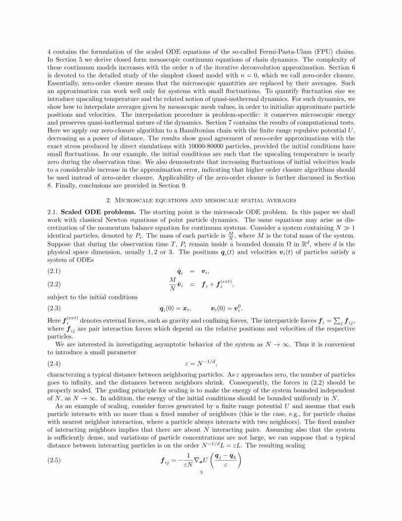
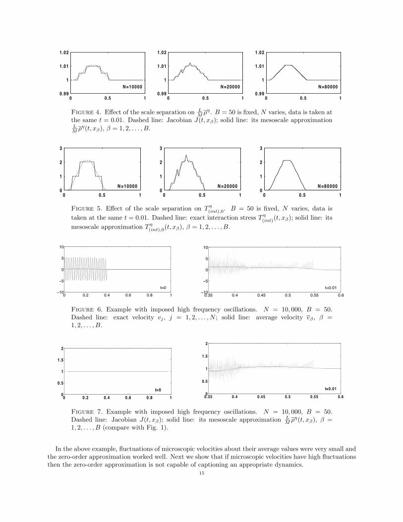
We next tested the effect of the scale separation on the quality of the zero-order approximation. Withfixed B = 50, we allowed N vary from 10, 000 to 80, 000 and followed the evolution of mesoscale quantities ofinterest: L

M ρη(t, xβ) and T η(int),0(t, xβ). Snapshots of these functions at the same representative time t = 0.01

are plotted in Figs. 4 and 5, respectively, with N = 10, 000, N = 20, 000 and N = 80, 000. The results withN = 40, 000 at the same time are given the middle top panels in Figs. 1, 2 for comparison. It is clear that asscale separation increases, oscillations in both L

M ρη(t, xβ) and T η(int),0(t, xβ) diminish and when N = 80, 000,

the exact microscopic quantities and their mesoscale approximations are almost indistinguishable.14

0 0.5 10.99

1

1.01

1.02

N=10000

0 0.5 10.99

1

1.01

1.02

N=20000

0 0.5 10.99

1

1.01

1.02

N=80000

Figure 4. Effect of the scale separation on LM ρη. B = 50 is fixed, N varies, data is taken at

the same t = 0.01. Dashed line: Jacobian J(t, xβ); solid line: its mesoscale approximationLM ρη(t, xβ), β = 1, 2, . . . , B.

0 0.5 10

1

2

3

N=10000

0 0.5 10

1

2

3

N=20000

0 0.5 10

1

2

3

N=80000

Figure 5. Effect of the scale separation on T η(int),0. B = 50 is fixed, N varies, data is

taken at the same t = 0.01. Dashed line: exact interaction stress T η(int)(t, xβ); solid line: its

mesoscale approximation T η(int),0(t, xβ), β = 1, 2, . . . , B.

0 0.2 0.4 0.6 0.8 1−10

−5

0

5

10

t=0

0.35 0.4 0.45 0.5 0.55 0.6−10

−5

0

5

10

t=0.01

Figure 6. Example with imposed high frequency oscillations. N = 10, 000, B = 50.Dashed line: exact velocity vj , j = 1, 2, . . . , N ; solid line: average velocity vβ , β =1, 2, . . . , B.

0 0.2 0 .4 0 .6 0 .8 10

0.5

1

1.5

2

t=00.35 0.4 0 .45 0.5 0 .55 0.60

0.5

1

1.5

2

t=0 .01

Figure 7. Example with imposed high frequency oscillations. N = 10, 000, B = 50.Dashed line: Jacobian J(t, xβ); solid line: its mesoscale approximation L

M ρη(t, xβ), β =1, 2, . . . , B (compare with Fig. 1).

In the above example, fluctuations of microscopic velocities about their average values were very small andthe zero-order approximation worked well. Next we show that if microscopic velocities have high fluctuationsthen the zero-order approximation is not capable of captioning an appropriate dynamics.

15

We demonstrate this by imposing high frequency k oscillations with relatively large amplitude a on thenonzero portion of the initial velocity used in the previous experiments. The initial velocity is

v0j =

γ + a sin( 5kπ

L q0j ), if 0 ≤ q0

j ≤ L5 ,

γ(− 5Lq

0j + 2

)+ a sin( 5kπ

L q0j ), if L

5 ≤ q0j ≤ 2L

5 ,

0, if 2L5 ≤ q

0j ≤ L.

and it is plotted in the left panel of Fig. 6. We use a = 5 and k = 20 that gives one period of imposedoscillations per mesocell. This microscopic initial velocity has a property that the average velocity at timet = 0 is exactly the same as in the previous example. Simulations were done with N = 10, 000 until thesame t = 0.07.

0 0.5 10

20

40

t=0

0 0.5 10

20

40

t=0.01

0 0.5 10

20

40t=0.02

0 0.5 10

20

40

x

t=0.03

0 0.5 10

20

40

x

t=0.05

0 0.5 10

20

40

x

t=0.07

Figure 8. Example with imposed high frequency oscillations. N = 10, 000, B = 50.Dashed line: exact interaction stress T η(int)(t, xβ); solid line: its mesoscale approximation

T η(int),0(t, xβ) (compare with Fig. 2).

The right panel of Fig. 6 shows a typical microscopic velocity profile together with its average velocity(taken at t = 0.01): to the left from the wave front, the microscopic velocity has large frequency oscillations(due to dispersion?) with an amplitude sometimes exceeding the initial amplitude by a factor of 1.5 and tothe right from the wave front, the microscopic velocity is zero. Clearly, the average velocity is very differentfrom the microscopic velocity.

Analysis of microscopic Jacobian J(t, xβ) and mesoscopic LM ρη(t, xβ) reveals that these functions have

qualitatively the same dynamics as micro- and mesoscale velocities, respectively, shown in Fig. 6. We plotthe former in Fig. 7 where the left panel has graphs at t = 0 while the right panel shows typical structurewith data taken at t = 0.01. It is interesting to note that the zero-order approximation T η(int),0(t, xβ) to

the interaction stress T η(int)(t, xβ) plotted in Fig. 8 does not agree in those areas that were affected by large

magnitude oscillations in microscopic velocities while agrees well in those areas to which oscillations havenot come yet. This finding suggests that indeed the zero-order approximation should not be used for largefrequency oscillations in microscopic velocities and a higher order approximation is needed.

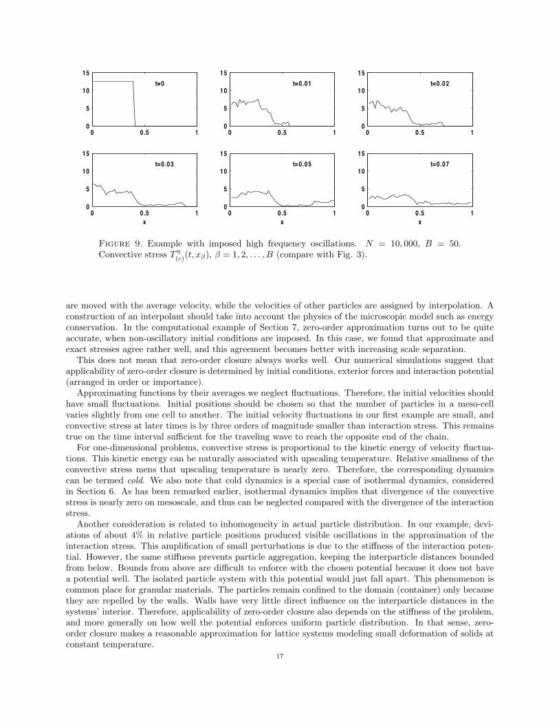
Finally, in Fig. 9 we plot the convective stress T η(c)(t, xβ) whose large values confirm that oscillations

in microscopic velocities are much bigger during the computational time than those in the first example.When the initial velocity has fluctuations with frequency higher than k = 20, discrepancy between micro-and mesoscale quantities is even more pronounced.

8. Zero-order closure: applicability

Zero-order closure is very similar to the use of the Cauchy-Born rule in quasi-continuum simulations ofsolids. Here, the nodes of the mesoscale mesh can be thought of as ”representative particles”. These particles

16

0 0.5 10

5

10

15

t=0

0 0.5 10

5

10

15

t=0.01

0 0.5 10

5

10

15

t=0.02

0 0.5 10

5

10

15

x

t=0.03

0 0.5 10

5

10

15

x

t=0.05

0 0.5 10

5

10

15

x

t=0.07

Figure 9. Example with imposed high frequency oscillations. N = 10, 000, B = 50.Convective stress T η(c)(t, xβ), β = 1, 2, . . . , B (compare with Fig. 3).

are moved with the average velocity, while the velocities of other particles are assigned by interpolation. Aconstruction of an interpolant should take into account the physics of the microscopic model such as energyconservation. In the computational example of Section 7, zero-order approximation turns out to be quiteaccurate, when non-oscillatory initial conditions are imposed. In this case, we found that approximate andexact stresses agree rather well, and this agreement becomes better with increasing scale separation.

This does not mean that zero-order closure always works well. Our numerical simulations suggest thatapplicability of zero-order closure is determined by initial conditions, exterior forces and interaction potential(arranged in order or importance).

Approximating functions by their averages we neglect fluctuations. Therefore, the initial velocities shouldhave small fluctuations. Initial positions should be chosen so that the number of particles in a meso-cellvaries slightly from one cell to another. The initial velocity fluctuations in our first example are small, andconvective stress at later times is by three orders of magnitude smaller than interaction stress. This remainstrue on the time interval sufficient for the traveling wave to reach the opposite end of the chain.

For one-dimensional problems, convective stress is proportional to the kinetic energy of velocity fluctua-tions. This kinetic energy can be naturally associated with upscaling temperature. Relative smallness of theconvective stress mens that upscaling temperature is nearly zero. Therefore, the corresponding dynamicscan be termed cold. We also note that cold dynamics is a special case of isothermal dynamics, consideredin Section 6. As has been remarked earlier, isothermal dynamics implies that divergence of the convectivestress is nearly zero on mesoscale, and thus can be neglected compared with the divergence of the interactionstress.

Another consideration is related to inhomogeneity in actual particle distribution. In our example, devi-ations of about 4% in relative particle positions produced visible oscillations in the approximation of theinteraction stress. This amplification of small perturbations is due to the stiffness of the interaction poten-tial. However, the same stiffness prevents particle aggregation, keeping the interparticle distances boundedfrom below. Bounds from above are difficult to enforce with the chosen potential because it does not havea potential well. The isolated particle system with this potential would just fall apart. This phenomenon iscommon place for granular materials. The particles remain confined to the domain (container) only becausethey are repelled by the walls. Walls have very little direct influence on the interparticle distances in thesystems’ interior. Therefore, applicability of zero-order closure also depends on the stiffness of the problem,and more generally on how well the potential enforces uniform particle distribution. In that sense, zero-order closure makes a reasonable approximation for lattice systems modeling small deformation of solids atconstant temperature.

17

To further understand limitations of zero-order closure, consider the effect of increasing the order n of theLandweber approximations (3.7). The Fourier transform the kernel of I −Rη is equal to

1− e−η2π2ξ·ξ.

It is very small for ξ close to zero, and then increases to one as |ξ| goes to infinity. Therefore, I −Rη acts asa filter damping low frequencies and thus emphasizing higher frequency content of the signal. Higher orderapproximations amount to applying convolutions

∑nk=1(I−Rη)k to mesoscale averages. As n increases, high

frequency content of the reconstruction will be increasingly amplified. This suggests that systems capableof producing large fluctuations should be handled with higher order approximations.

A related comment is that averages of fluctuations can become additional state variables in a mesoscalecontinuum model. A familiar example is the use of the averaged energy balance equation (see [1] for deriva-tion), in addition to the mass and momentum balance. The energy balance equation describes evolution ofthe density of kinetic energy of velocity fluctuations. An intriguing question here is how the model with justtwo equations of balance but high order closure approximation compares with a zero-order closure modelcontaining all three balance equations. In classical physics, additional balance equations are often introducedas a means of compensating for errors introduced by replacing state variables with their averages. Use ofhigher order closure could offer an alternative to this approach. Indeed, suppose that one is interested onlyin tracking density and velocity on mesoscale. The corresponding two balance equations contain only twomicroscale quantities: velocity field v and the Jacobian J of the inverse position map q−1. If v and J can beaccurately reconstructed from their averages, we do not need to deal with the energy balance equation. Thisobservation offers a new way of reducing computational cost. Higher order approximation are more expen-sive than zero-order, but using more balance equations also increases computational cost. We also note thatincreasing the order of closure approximations involves repeated convolutions with the window function ψη.On the other hand, simulating an energy balance involves numerical integration of an additional non-linearintegral-differential equation, a much more difficult task.

9. Conclusions

We propose a closure method that gives closed form approximations for mesoscale continuum mechanicalfluxes (such as stress) in terms of primary mesoscopic variables (such as average density and velocity). Ourclosure construction is based on iterative regularization methods for solving first kind integral equations.Such integral equations are relevant because mesoscopic density and velocity are related to the correspondingmicroscopic quantities via a linear convolution operator. The problem of inverting convolution operators isunstable (ill-posed) and requires regularization. Use of the well known Landweber iterative regularizationyields successive approximations, of orders zero, one, two and so forth, to interpolants of particle positionsand velocities in terms of available averages. Closure is achieved by inserting any of these approximationsinto the equations for fluxes instead of the actual particle positions and velocities. Low order approximationsare simpler to implement, while higher order approximations can be used to more accurately reproduce thehigh frequency content of the microscopic quantities.

The above general strategy is applied in the paper to spatially averaged dynamics of classical particlechains. We focus on the simplest zero-order approximation and show numerically that it works reasonablywell as long as initial conditions have small velocity fluctuations. The case of large fluctuations in velocitiesshould be handled by higher order approximations.

10. Acknowledgments

Work of Alexander Panchenko was supported in part by DOE grant DE-FG02-05ER25709 and by NSFgrant OISE-0438765. Work of R. P. Gilbert was supported in part by NSF grants OISE-0438765 and DMS-0920850, and by the Alexander v. Humboldt Senior Scientist Award at the Ruhr Universitat Bochum.

References

[1] Murdoch, A. I. and Bedeaux, D. Continuum equations of balance via weighted averages of microscopic quantities Proc.

Royal Soc. London A (1994), 445, 157–179.

18

[2] Murdoch, A. I. and Bedeaux, D. A microscopic perpsective on the physical foundations of continuum mechanics–Part I:macroscopic states, reproducibility, and macroscopic statistics, at presctribed scales of length and time Int. J. Engng Sci.

Vol. 34, No. 10 (1996), 1111-1129.

[3] Murdoch, A. I. and Bedeaux, D. A microscopic perpsective on the physical foundations of continuum mechanics II: aprojection operator approach to the separation of reversible and irreversible contributions to macroscopic behaviour Int. J.

Engng Sci. Vol. 35, No. 10/11 (1997), 921-949.

[4] Murdoch, A. I. A Critique of Atomistic Definitions of the Stress Tensor J Elasticity (2007), 88, 113–140.[5] Fridman V. A method of successive approximations for Fredholm integral equations of the first kind (Russian). Uspekhi

Mat. Nauk, 11 (1956), 233-234.[6] C. W. Groetsch. The Theory of Tikhonov Regularization for Fredholm Equation of the First Kind. Pitman, Boston, (1984).

[7] Hanke M. Accelerated Landweber iterations for the solution of ill-posed equations. Numer. Math. , 60, (1991), 341373.

[8] Hanke M. Regularization with differential operators: an iterative approach. Numer. Func. Anal. Optim. 13, (1992), 523540.[9] Kirsch A. An Introduction to the Mathematical Theory of Inverse Problems. Springer, New York, (1996).

[10] Landweber L. An iteration formula for Fredholm integral equations of the first kind. Am. J. Math., 73 (1951), 615-624.

[11] Engl H. W. On the choice of the regularization parameter for iterated Tikhonov regularization of ill-posed problems J.Approx. Theory. (1987), 49, 5563.

[12] Engl H. W. , Hanke M. , and Neubauer A. Regularization of Inverse Problems. Dordrecht: Kluwer Academic, (1996).

[13] Hardy, R.J. Formulas for determining local properties in molecular-dynamics simulations: shock waves. J. Chem. Phys. 76(1982), 622628.

[14] Irving J.H., and Kirkwood, J.G. The statistical theory of transport processes IV. The equations of hydrodynamics. J.

Chem. Phys. 18 (1950), 817829.[15] Morozov V. A. Methods for Solving Incorrectly Posed Problems. Springer, New York, (1984).

[16] Noll, W. Der Herleitung der Grundgleichungen der Thermomechanik der Kontinua aus der statistischen Mechanik. J.Ration. Mech. Anal. 4, (1955), 627646.

[17] G.A. Pavliotis and A. M. Stuart. Multiscale methods. Averaging and homogenization, Springer 2008.

[18] Tikhonov A. N. and Arsenin V. Y. Solutions of Ill-Posed Problems. New York: Wiley (1987).

Department of Mathematics, Washington State University, Pullman, WA 99164E-mail address: panchenko@math.wsu.edu

Department of Mathematics University of Idaho, Moscow, ID 83843E-mail address: barannyk@uidaho.edu

Department of Mathematical Sciences, University of Delaware, Newark, DE 19716

E-mail address: gilbert@math.edul.edu

19