Spatially discrete metapopulation models with directional dispersal

www.elsevier.com/locate/mbs

Mathematical Biosciences 204 (2006) 68–101

Spatially discrete metapopulation modelswith directional dispersal

Abdul-Aziz Yakubu a,*, Michael J. Fogarty b

a Department of Mathematics, Howard University, Washington, DC 20059, United Statesb National Oceanic and Atmospheric Administration, National Marine Fisheries Service,

Northeast Fisheries Science Center, Woods Hole, MA 02543, United States

Received 6 October 2005; received in revised form 1 May 2006; accepted 31 May 2006Available online 30 June 2006

Abstract

We use an age-structured discrete-time metapopulation model linking two sub-populations through lar-val transport and directed movements of adults to study the implications of linkages among subpopulationsfor the stability and resilience of exploited species. Our two-habitat model, a generalization of Fogarty’sinshore–offshore lobster population model, includes isolated habitats under compensatory (monotone)or overcompensatory (oscillatory) dynamics [M.J. Fogarty, Implications of migration and larval inter-change in American lobster (Homarus americanus) stocks: spatial structure and resilience, in: G.S. Jamie-son, A. Campbell (Eds.), Proc. of North Pacific Symposium on Invertebrate Stock Assessment andManagement, Can. Spec. Publ. Fish. Aquat. Sci. 125 (1998) 273]. Pre-migration local dynamics are selectedfrom general classes of functions that capture the effects of competition for resources via contest (compen-satory) and scramble (overcompensatory) intraspecific competitions. We explore the implications of thesemechanisms on the long-term survival of exploited species. In particular, we use threshold parameters R1

d

for Habitat 1 and R2d for Habitat 2 together with precise mathematical definitions to prove that species per-

sistence is possible at high levels of fishing in one habitat and low to moderate levels of fishing in the other.Our results support Fogarty’s conclusion that conservative management of larval source populations couldcontribute to the resilience of exploited species.� 2006 Elsevier Inc. All rights reserved.

0025-5564/$ - see front matter � 2006 Elsevier Inc. All rights reserved.doi:10.1016/j.mbs.2006.05.007

* Corresponding author. Tel.: +1 202 806 6830; fax: +1 202 806 6831.E-mail addresses: [email protected] (A.-A. Yakubu), [email protected] (M.J. Fogarty).

mailto:[email protected]

mailto:[email protected]

A.-A. Yakubu, M.J. Fogarty / Mathematical Biosciences 204 (2006) 68–101 69

Keywords: Age-structured model; Compensatory dynamics; Inshore–offshore system; Larval transport; Migration;Overcompensatory dynamics

1. Introduction

Fish populations have complex life-history dynamics, and the causes of this complexity aremany and varied. Typically, fish vital rates are density-dependent, age and size specific, andrecruitment is subject to environmental stochasticity. The populations are often subdivided inspace, spread among habitats of highly variable quality that are connected via larval transportand adult migration. These factors when coupled with exploitation via fishing activities makelong-term predictions of life-history dynamics seem intractable [14–18].

Coastal American lobster (Homarus americanus) stocks exhibit strong resilience to exploitation(resilience is defined as the capacity of the population to withstand a sustained perturbation viafishing). In 1998, Fogarty used a discrete-time inshore–offshore age-structured lobster populationmodel to study the implications of linkages between lobster groups for the stability and resilienceof exploited stocks, where larval populations are governed by the Beverton–Holt model. Fogartyfound, that the observed resilience of the American lobster may be attributable to strong compen-satory mechanisms, the effects of larval subsidies from offshore lobster groups, or a combinationof both mechanisms [16,59]. In this paper, we introduce a discrete-time age-structured metapop-ulation model linking two subpopulations through larval transport and directed movements ofadults [1,3,9–12,21–28]. In our model, larval populations are governed by either compensatory(equilibrium or monotone) or overcompensatory (oscillatory or non-monotone) dynamics [5–7,29–32,52,54,57–59]. The model, a generalization of Fogarty’s inshore–offshore lobster popula-tion model, tracks populations rather than probabilities of patch occupancy [16]. As in Fogarty’smodel, in our model dispersal arises from deterministic directed motion rather than stochasticcolonization.

Classical metapopulation theory is framed by the dynamic interplay of extinction and recolo-nization events (e.g. [43,25]). In this paper, we adopt the more general definition of a metapopu-lation as a number of populations distributed over space, linked through dispersal processes (e.g.[28,38]). Fogarty and Botsford, in [19], examined the applicability of this broader definition toempirical evidence for a number of decapod crustaceans including the American lobster.

Spatial heterogeneity is an important aspect of the biological and physical processes that gov-ern fish population dynamics. Mathematical ecologists have had great success in showing howspecific aspects of the spatial environment alters population and community environment.However, most of the existing fisheries models that are used for research and fisheries manage-ment are non-spatial [2,4,8,14–19,35,39,40,47,54]. The age-structured two-habitat model for thisstudy has a spatial structure, and the model equations capture the effects of contest and scrambleintraspecific competitions via compensatory and overcompensatory dynamics, respectively[3,7,13,29,30,34,52,54].

Cobb et al. [8], Fogarty [16], Rogers et al. [56] and others have documented the importance oflarval subsidies to heavily exploited inshore lobster groups. For example, offshore lobsters fromthe Browns Bank region serve as a source of larvae to coastal Nova Scotia stocks [14–18]. Ourtwo-habitat larval-adult model has larval transport from one habitat to the other.

70 A.-A. Yakubu, M.J. Fogarty / Mathematical Biosciences 204 (2006) 68–101

In this paper, we focus on the influence of various assumptions (such as whether the dynamicsof the isolated habitats are monotone (compensatory) or oscillatory (overcompensatory), fishinglevels, migration levels and survival rates) on the metapopulation dynamics. We derive the basicreproductive numbers (threshold parameters), R1

d on Habitat 1 and R2d on Habitat 2, and use pre-

cise mathematical definitions of compensatory and overcompensatory dynamics to make long-term predictions in the dispersal-linked two-habitat model. When the isolated (local) dynamicsare either compensatory or overcompensatory, Ri

d > 1 guarantees the successful invasion and sur-vival of Habitat i 2 {1,2} population while Ri

d < 1 guarantees the extinction of the initial popu-lation, where there is no migration between the two habitats. As observed by Fogarty [16], thespecies survives on a globally attracting fixed point when the larval populations are under com-pensatory dynamics. However, it exhibits single or multiple cyclic attractors or chaotic attractorswhen the dynamics are overcompensatory. High level of exploitation weakens the resilience ofboth subpopulations, and it is also capable of shifting the qualitative dynamics from multipleattractors to a single attractor.

Without transport of larvae between the subpopulations, we obtain that high levels of adultmigration from Habitat 1 to Habitat 2 can eventually lead to Habitat 1 population extinctionwhile the Habitat 2 population is sustained. When there is larval exchange from Habitat 2 toHabitat 1 group and all Habitat 1 adults are sedentary, then R1

d < 1 and R2d < 1 imply extinction

of the species in both habitats. However, R2d > 1 implies persistence of both Habitats 1 and 2

populations. We use numerical simulations to highlight that larval transport can shift the qual-itative dynamics of metapopulation models with directed movement of adults from multipleattractors with complex (fractal) basins of attraction to single attractors with simpler basins ofattraction.

Section 2 is on pre-migration unstructured closed population models. These models are used todescribe pre-migration local population dynamics on two (uncoupled) natal regions, Habitat 1and Habitat 2. These one-dimensional models are used to give precise definitions of compensatoryand overcompensatory dynamics in populations. In Section 3, we develop our main model, a twohabitat (Habitat 1 and Habitat 2) age-structured (larvae-adults) discrete-time system in which theHabitat 1 group receives a larval subsidy from Habitat 2. The adults from Habitat 1 undertake adirectional migration to Habitat 2. A threshold parameter, R1

d , for the persistence or extinction ofpre-migration Habitat 1 population is introduced in Section 4, where the larval population is un-der compensatory or overcompensatory dynamics.

Section 5 is on the two-habitat system with adult migration but without larval exchange.The impact of compensatory and overcompensatory dynamics on the stability and resilienceof the species in this sub-system are discussed in Section 5. We show, in Section 6, that ahigh level of fishing can shift the system dynamics from complex basin-boundary structures tosingle attractors with relatively simple basins of attraction. The role of compensatory andovercompensatory dynamics in the full model with larval transport are also explored in Section6. We show that low to moderate levels of fishing pressure in Habitat 2 coupled with low tomoderate levels of larval exchange can save Habitat 1 population from extinction. As in Section5, we demonstrate that larval transport can also shift the system dynamics from multiple attrac-tors with complex basin-boundary structures to single attractors with relatively simple basins ofattraction. Our results are summarized in Section 7, and detailed proofs are collected in theAppendix.


2. Pre-migration local habitat population dynamics

The local dynamics of the unstructured population in each Habitat i 2 {1,2} after reproductionbut before migration is modeled by the general equation

xiðtÞ ¼ fiðxiðt � 1ÞÞ ði ¼ 1; 2Þ; ð1Þ

where xi(t) denotes the population size at generation t. The pre-migration Habitat i local function,fi(xi) = xigi(xi), describes the local dynamics of the species where the per-capita growth functions,gi : [0,1)! (0,1), are assumed to be strictly decreasing, positive, smooth, gi(0) > 1, andgi(xi)! 0 as xi!1.

Each fi has a unique positive fixed point denoted by Xi. Since gi is a strictly decreasing contin-uous function then fi(xi) > xi whenever 0 < xi < X and fi(xi) < xi whenever xi > Xi. Model (1) is adiscrete-time, single-species, closed unstructured population model with two (uncoupled) natalregions. It describes the population dynamics of pioneer species (pioneer species thrive at lowpopulation densities, gi(0) > 1 [20,39,57,58]).

The following definitions will be used to study the long-term dynamics of initial populationsizes under fi iterations. We write the definitions for any continuous function

f : M ! M ;

where M is a metric space [37,39,55,59].

Definition 1. A compact invariant set I �M is called a trapping region for f whenever f(I) � int(I)[55].

Definition 2. A set K is called an attracting set (or an attractor) provided there is a trapping regionI �M such that K = \kP0fk(I) [55].

When K attracts every point in the interior of M we say it is a global attractor. By ourdefinitions,

I i ¼ fið½0;X i�Þ ð2Þ

is a global attractor. That is, eventually every initial population size in model (1) is attracted to Ii

[7,20,39,57,58].We focus on two types of local dynamics, compensatory and overcompensatory dynamics (def-

initions are given below).

Definition 3. Habitat i pre-migration local dynamics are compensatory whenever all positivepopulation sizes approach the positive equilibrium at Xi monotonically under fi iterations[7,57,58].

If fi increases monotonically from zero with the rate of increase slowing down as xi gets large,then all population sizes ‘undershoot’ the globally attracting positive equilibrium, and by Defini-tion 3 Habitat i local dynamics are compensatory. The Beverton–Holt stock recruitment modelused in Fogarty’s study [16], fiðxiÞ ¼ aixi

1þbixi, portrays compensatory dynamics in Habitat i where

the positive constant ai > 1 is the maximal per-capita intrinsic growth rate of the population


and the positive constant bi scales the carrying capacity of the population, X i ¼ ai�1bi

[3–6,24,29–31,39,48–54].

Observe that when fiðxiÞ ¼ aixi1þbixi

, then f 0i ðxiÞ > 0 and f 00i ðxiÞ < 0 for each xi 2 [0,1). We use thefollowing definition to classify natal regions under compensatory dynamics.

Definition 4. The local dynamics in Habitat i, fi is a monotone map if f 0i ðxiÞ > 0 for eachxi 2 [0,1) [7,57,58].

Since the origin is an unstable fixed point of fi ðf 0i ð0Þ > 1Þ, Habitat i pre-migration localdynamics are compensatory whenever fi is a monotone map with its unique positive fixed pointXi. The conditions in Definition 4 are sufficient but not necessary for compensatory dynamicsin the pre-migration local habitat population.

Definition 5. Habitat i pre-migration local dynamics are overcompensatory whenever somepositive population sizes ‘overshoot’ the positive equilibrium at Xi under fi iterations (that is,f 0i ðX iÞ < 0) [7,57,58].

A mechanism that can lead to overcompensatory dynamics is cannibalism of juveniles byadults. If fi is an orientation-reversing one hump map with a stable positive fixed point (respec-tively, an unstable positive fixed point), then the return to the stable fixed point takes the formof damped oscillations (respectively, the local behavior near the unstable fixed point takes theform of divergent oscillations), and by Definition 5 natal region i dynamics are overcompensatory.Also, if fi is an orientation-reversing one hump map with an unstable positive fixed point, then thelocal behavior near the unstable fixed point takes the form of divergent oscillations, and by Def-inition 5 natal region i dynamics are overcompensatory. Whenever the carrying capacity of thepopulation ri > 1 and fi is Ricker’s model, fi(xi) = xi exp(ri � xi), then the dynamics in Habitat iare overcompensatory [48–54,57–59]. In general, fi supports either an n-cycle (non-chaotic) attrac-tor with n > 1 or a chaotic (interval) attractor whenever Habitat i dynamics are overcompensatoryand the positive fixed point is unstable.

3. Two-habitat systems with a larval subsidy from Habitat 1 to 2

In 1998, Fogarty studied an age-structured, discrete-time, inshore–offshore system with a larvalsubsidy from the offshore to the inshore subpopulation where migration is unidirectional [16].Adults migrate from inshore to offshore habitat while a fraction of the larvae produced by theoffshore subpopulation are transported inshore (see Fig. 1). In Fogarty’s lobster population mod-el, the adult migration follows the period of larval release. The model assumed a time delay of fiveyears between the egg stage and recruitment to the adult population (reproductive delay). How-ever, sensitivity analysis showed that the qualitative dynamics are independent of the length of thereproductive delay [16].

To state Fogarty’s model, for each Habitat i 2 {1,2}, let xi(t) be the number of adults at time t.In the ith subpopulation, di is the proportion of non-migratory adults, ci is the proportion of pre-recruits that remain in the natal region, and qi is the adult survivorship. Fogarty’s specific modelwith a reproductive delay of two years is given by the following system of non-linear delay-differ-ence equations:

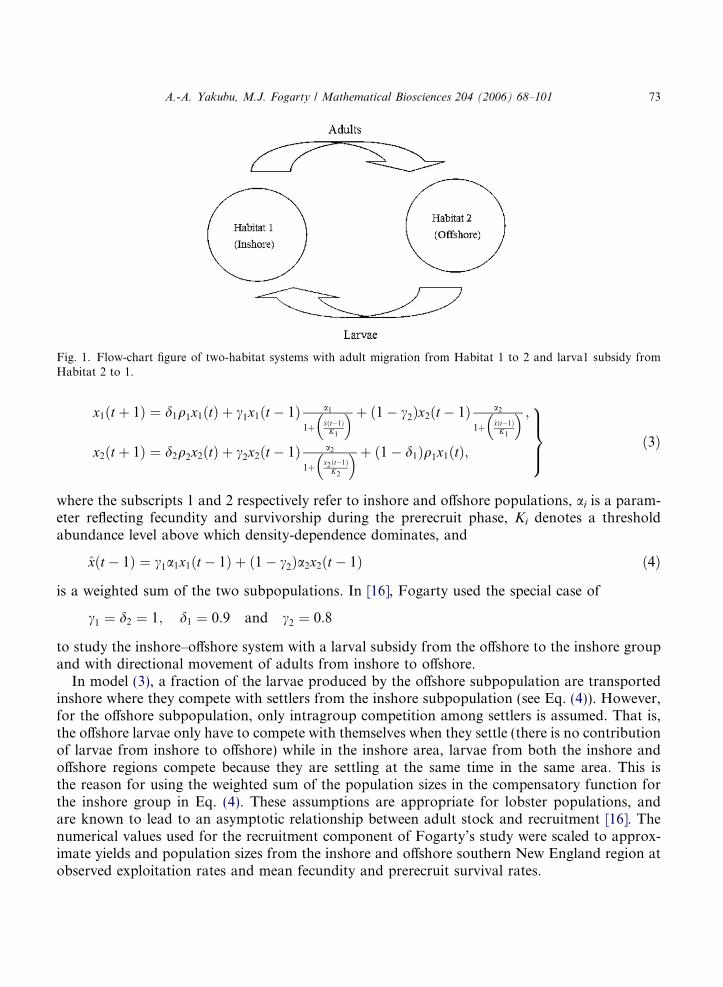
Fig. 1. Flow-chart figure of two-habitat systems with adult migration from Habitat 1 to 2 and larva1 subsidy fromHabitat 2 to 1.


x1ðt þ 1Þ ¼ d1q1x1ðtÞ þ c1x1ðt � 1Þ a1

1þ xðt�1ÞK1

� �þ ð1� c2Þx2ðt � 1Þ a2

1þ xðt�1ÞK1

� � ;x2ðt þ 1Þ ¼ d2q2x2ðtÞ þ c2x2ðt � 1Þ a2

1þ x2ðt�1ÞK2

� �þ ð1� d1Þq1x1ðtÞ;

9>>=>>; ð3Þ

where the subscripts 1 and 2 respectively refer to inshore and offshore populations, ai is a param-eter reflecting fecundity and survivorship during the prerecruit phase, Ki denotes a thresholdabundance level above which density-dependence dominates, and

xðt � 1Þ ¼ c1a1x1ðt � 1Þ þ ð1� c2Þa2x2ðt � 1Þ ð4Þ

is a weighted sum of the two subpopulations. In [16], Fogarty used the special case of

c1 ¼ d2 ¼ 1; d1 ¼ 0:9 and c2 ¼ 0:8

to study the inshore–offshore system with a larval subsidy from the offshore to the inshore groupand with directional movement of adults from inshore to offshore.

In model (3), a fraction of the larvae produced by the offshore subpopulation are transportedinshore where they compete with settlers from the inshore subpopulation (see Eq. (4)). However,for the offshore subpopulation, only intragroup competition among settlers is assumed. That is,the offshore larvae only have to compete with themselves when they settle (there is no contributionof larvae from inshore to offshore) while in the inshore area, larvae from both the inshore andoffshore regions compete because they are settling at the same time in the same area. This isthe reason for using the weighted sum of the population sizes in the compensatory function forthe inshore group in Eq. (4). These assumptions are appropriate for lobster populations, andare known to lead to an asymptotic relationship between adult stock and recruitment [16]. Thenumerical values used for the recruitment component of Fogarty’s study were scaled to approx-imate yields and population sizes from the inshore and offshore southern New England region atobserved exploitation rates and mean fecundity and prerecruit survival rates.


In Fogarty’s model (3),

TableA tab

Param

ai

di

qi

ci

Ki

ai andMi

Fi

fiðxiÞ ¼ xiai

1þ c1a1x1þð1�c2Þa2x2

Ki

� �
are the functions relating adult population size and recruitment from the different sources. In theabsence of the offshore (inshore) population, f1 (f2) reduces to the Beverton–Holt stock recruit-ment model. That is, only compensatory dynamics are considered in model (3). To study the ef-fects of both compensatory and overcompensatory mechanisms and the importance of migrationon the persistence of exploited species, we consider Fogarty’s model (3) with a more general per-capita growth rate for each ith subpopulation, gi : [0,1)! (0,1). The model for our study is
x1ðt þ 1Þ ¼ d1q1x1ðtÞ þ c1x1ðt � 1Þg1ð�xðt � 1ÞÞ þ ð1� c2Þx2ðt � 1Þg2ð�xðt � 1ÞÞ;x2ðt þ 1Þ ¼ d2q2x2ðtÞ þ c2x2ðt � 1Þg2ðc2g2ð0Þx2ðt � 1ÞÞ þ ð1� d1Þq1x1ðtÞ;

�ð5Þ

where

�xðt � 1Þ ¼ c1g1ð0Þx1ðt � 1Þ þ ð1� c2Þg2ð0Þx2ðt � 1Þ: ð6Þ
In model (5), adult survivorship
qi ¼ e�ðMiþF iÞ; ð7Þ
where Mi is the instantaneous rate of natural mortality and Fi is the fishing mortality. To study theimplications of increased probability of movement with increasing abundance, the proportion ofnon-migratory adults
di ¼ expð�ai � bixiÞ; ð8Þ
where the constants ai > 0 and bi P 0 are the instantaneous movement coefficients (see Table 1).To simplify our analysis, we assume throughout that bi = 0 so that di is constant in each Habitati 2 {1,2}. As in the previous section, the effective per-capita growth functions, gi : [0,1)! (0,1),are assumed to be strictly decreasing, positive and smooth, where gi(0) > 1, and gi(xi)! 0 asxi!1.
Model (5) reduces to Fogarty’s lobster model, model (3), whenever giðxiÞ ¼ ai1þbixi

(compensatorydynamics) [16]. However, when gi(xi) = exp(ri � xi) then the prerecruits exhibit overcompensatorydynamics via the Ricker model.

1le of parameters

eter in Habitat i Description

Maximum growth rate during the prerecruit phaseProportion of non-migratory adultsAdult survival rateProportion of prerecruits that remain in the natal Habitat i

Threshold abundance levelbi Instantaneous movement coefficients

Natural mortalityFishing mortality


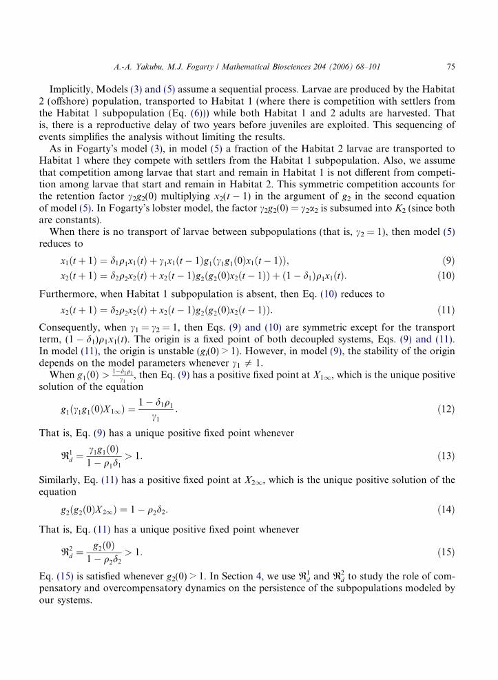
Implicitly, Models (3) and (5) assume a sequential process. Larvae are produced by the Habitat2 (offshore) population, transported to Habitat 1 (where there is competition with settlers fromthe Habitat 1 subpopulation (Eq. (6))) while both Habitat 1 and 2 adults are harvested. Thatis, there is a reproductive delay of two years before juveniles are exploited. This sequencing ofevents simplifies the analysis without limiting the results.

As in Fogarty’s model (3), in model (5) a fraction of the Habitat 2 larvae are transported toHabitat 1 where they compete with settlers from the Habitat 1 subpopulation. Also, we assumethat competition among larvae that start and remain in Habitat 1 is not different from competi-tion among larvae that start and remain in Habitat 2. This symmetric competition accounts forthe retention factor c2g2(0) multiplying x2(t � 1) in the argument of g2 in the second equationof model (5). In Fogarty’s lobster model, the factor c2g2(0) = c2a2 is subsumed into K2 (since bothare constants).

When there is no transport of larvae between subpopulations (that is, c2 = 1), then model (5)reduces to

x1ðt þ 1Þ ¼ d1q1x1ðtÞ þ c1x1ðt � 1Þg1ðc1g1ð0Þx1ðt � 1ÞÞ; ð9Þx2ðt þ 1Þ ¼ d2q2x2ðtÞ þ x2ðt � 1Þg2ðg2ð0Þx2ðt � 1ÞÞ þ ð1� d1Þq1x1ðtÞ: ð10Þ

Furthermore, when Habitat 1 subpopulation is absent, then Eq. (10) reduces to

x2ðt þ 1Þ ¼ d2q2x2ðtÞ þ x2ðt � 1Þg2ðg2ð0Þx2ðt � 1ÞÞ: ð11Þ
Consequently, when c1 = c2 = 1, then Eqs. (9) and (10) are symmetric except for the transportterm, (1 � d1)q1x1(t). The origin is a fixed point of both decoupled systems, Eqs. (9) and (11).In model (11), the origin is unstable (gi(0) > 1). However, in model (9), the stability of the origindepends on the model parameters whenever c1 5 1.
When g1ð0Þ > 1�d1q1

c1, then Eq. (9) has a positive fixed point at X11, which is the unique positive

solution of the equation

g1ðc1g1ð0ÞX 11Þ ¼1� d1q1

c1

: ð12Þ

That is, Eq. (9) has a unique positive fixed point whenever

R1d ¼

c1g1ð0Þ1� q1d1

> 1: ð13Þ

Similarly, Eq. (11) has a positive fixed point at X21, which is the unique positive solution of theequation

g2ðg2ð0ÞX 21Þ ¼ 1� q2d2: ð14Þ

That is, Eq. (11) has a unique positive fixed point whenever

R2d ¼

g2ð0Þ1� q2d2

> 1: ð15Þ

Eq. (15) is satisfied whenever g2(0) > 1. In Section 4, we use R1d and R2

d to study the role of com-pensatory and overcompensatory dynamics on the persistence of the subpopulations modeled byour systems.


We use the following auxiliary results to study long-term dynamics in Eqs. (9) and (11).

Lemma 1. For each Habitat i 2 {1,2}, let max Ii be the positive (bigger) end-point of the closedinterval Ii � fi([0,Xi]).

(a) In Eq. (9),

x1ðt þ 1Þ 6x1ðtÞ þ x1ðt � 1Þ if c1g1ð0Þx1ðt � 1Þ > max I1;

x1ðtÞ þmax I1 if c1g1ð0Þx1ðt � 1Þ 2 I1:

�
(b) In Eq. (11),
x2ðt þ 1Þ 6x2ðtÞ þ x2ðt � 1Þ if g2ð0Þx2ðt � 1Þ > max I2;

x2ðtÞ þmax I2 if g2ð0Þx2ðt � 1Þ 2 I2:

�

Proof. Recall that qidi = qi exp(�ai � bixi) < 1, Ii � fi([0,Xi]) is fi-invariant and gi(xi) < 1 when-ever xi > Xi.

(a) If c1g1(0)x1 > max I1, then g1(c1g1(0)x1) < 1 and

x1ðt þ 1Þ 6 d1q1x1ðtÞ þ c1x1ðt � 1Þ:
That is,
x1ðt þ 1Þ 6 x1ðtÞ þ x1ðt � 1Þ:
Also, if c1g1(0)x1 2 I1 then c1g1(0)x1g1(c1g1(0)x1) 2 I1 and
g1ð0Þx1ðt þ 1Þ ¼ d1q1g1ð0Þx1ðtÞ þ c1g1ð0Þx1ðt � 1Þg1ðc1g1ð0Þx1ðt � 1ÞÞ6 g1ð0Þx1ðtÞ þmax I1

6 g1ð0Þx1ðtÞ þ g1ð0Þmax I1:

The proof of (b) is similar and is omitted. h

Lemma 2. In Eq. (9) or (11), if either

xið�1Þ > 0 or xið0Þ > 0;

then

xiðtÞ > 0 for all t P 1:

The proof of Lemma 2 is straightforward and is omitted.

Compensatory dynamics in the prerecruits of the offshore population described by Eq. (11) leadto compensatory dynamics in the adult population (in isolation) [58]. We summarize these in thefollowing result:

Theorem 1. Let Habitat 2 (pre-migration) local dynamics be compensatory, where f2 is a monotonemap. Then Eq. (11) has a globally attracting positive equilibrium at

X 21 ¼g�1

2 ð1� d2q2Þg2ð0Þ

:


That is, compensatory dynamics in Habitat 2 prerecruits lead to compensatory dynamics in Habitat 2adults, and every positive initial population size in the single habitat model (in isolation) is attractedto the positive fixed point, X21.

The Proof of Theorem 1 is in the Appendix.The following example, Example 1, shows that Eqs. (9) and (11) support multiple attractors

when either the proportion of non-migratory adults is small or the fishing mortality is high andthe prerecruits exhibit overcompensatory dynamics via the Ricker model. To illustrate this, wewrite Eq. (11) as a system of two first-order equations. That is, when x2(t � 1) = y2(t) then Eq.(11) becomes

Fig. 2M2 =verticacondit

x2ðt þ 1Þ ¼ d2q2x2ðtÞ þ 1g2ð0Þ

f2ðg2ð0Þy2ðtÞÞ;y2ðt þ 1Þ ¼ x2ðtÞ:

)ð16Þ

Example 1. Consider system (16) with

f2ðy2Þ ¼ y2 expðr2 � y2Þ;
where
a2 ¼ 5:809; r2 ¼ 2:6; M2 ¼ 0:05; and F 2 ¼ 0:

In Example 1, the constant proportion of non-migratory adults is small and there is no exploi-tation (no-take areas, refuges or reserves). Fig. 2 shows that, these combined with overcompen-satory dynamics generate multiple attractors via two coexisting 8-cycle attractors atapproximately

ð0:369; 0:368Þ ! ð0:036; 0:369Þ ! ð0:035; 0:036Þ ! ð0:298; 0:035Þ ! ð0:294; 0:298Þf! ð0:073; 0:294Þ; ð0:076; 0:073Þ; ð0:368; 0:076Þg

. System (16) supports two coexisting 8-cycle attractors in the adult–juvenile plane when a2 = 5.809, r2 = 2.6,0.05, F2 = 0, and f2(y2) = y2 exp(r2 � y2) (Example 1). On the horizontal (adult) axis, 0 6 x2 6 0.5 and on thel (juvenile) axis, 0 6 y2 6 0.5. The initial condition (0.01,0.01) converges to one 8-cycle attractor while the initialion (0.01,0.3) converges to the other attractor.


and

Fig. 3fixedaxis, 0

ð0:369; 0:298Þ ! ð0:074; 0:369Þ ! ð0:035; 0:074Þ ! ð0:368; 0:035Þ ! ð0:295; 0:368Þf! ð0:036; 0:295Þ; ð0:075; 0:036Þ; ð0:298; 0:075Þg;

respectively.To illustrate the importance of migration on life-history outcomes, we keep all other parame-

ters in Example 1 fixed at their original values while we vary d2, the proportion of non-migratoryoffshore adults, between 0 and 1. Fig. 3 shows that system (16) undergoes complex bifurcationsincluding period-doubling reversals and discrete-Hopf bifurcations. High fishing pressure canhave similar impact on life-history outcomes in Eq. (9) or (11).

We use the following precise persistence definition to illustrate species persistence in ourmodels.

Definition 6. In Eq. (9) or (11), the Habitat i 2 {1,2} population in isolation is persistent if

limt!1

inf xiðtÞ > 0;

whenever either xi(�1) > 0 or xi(0) > 0.

Lemma 2 does not guarantee species persistence. In the following result, we use Lemma 2 toprove that the presence of either larvae or adult species at some (initial) generation implies thepersistence of the population in that habitat.

Lemma 3. In Eq. (11), if either

x2ð�1Þ > 0 or x2ð0Þ > 0;

then the isolated population in Habitat 2 is persistent.

The Proof of Lemma 3 is in the Appendix.

. High values of d2 force period-doubling reversals and discrete-Hopf bifurcations, where all parameters are keptin Example 1 and d2 is varied between 0 and 1. On the horizontal (d2) axis, 0 6 d2 6 1. On the vertical (juvenile)6 x2 6 0.5.


4. Habitat 1 local population dynamics

In this section, we study Habitat 1 (pre-migration) local population growth where larval pop-ulations are governed by either compensatory (Beverton–Holt model) or overcompensatory(Ricker model) mechanisms.

4.1. Compensatory dynamics

The study of the role of compensatory processes on the resilience of the Habitat 1 subpopula-tion to exploitation can be simplified via the use of a threshold parameter. The basic demographicreproductive number of the Habitat 1 population (in the absence of larvae transport) is

R1d ¼

c1g1ð0Þ1� q1d1

;

R1d , a threshold parameter, gives the pre-larvae transport average number of offsprings produced

by a typically small initial Habitat 1 population (x1(0),x1(�1)) over their lifetime in the natalregion. In the absence of larvae transport, R1

d > 1 guarantees the successful invasion and survivalof the Habitat 1 population while R1

d < 1 guarantees the extinction of the initial inshore popula-tion. We summarize these in the following result.

Theorem 2. In Eq. (9), let Habitat 1 (pre-migration) local dynamics be compensatory, where f1 is amonotone map.

(a) If

R1d < 1;

then the zero fixed point is globally asymptotically stable, and the Habitat 1 population goes extinct.(b) If

R1d > 1;

then Eq. (9), has a globally asymptotically stable positive fixed point at

X 11 ¼1

c1g1ð0Þg�1

1

g1ð0ÞR1

d

!
and the Habitat 1 population persists on the fixed point attractor X11.
The Proof of Theorem 2 is in the Appendix.Since q1 ¼ e�ðM1þF 1Þ,

R1d ¼

c1g1ð0Þ1� e�ðM1þF 1Þd1

;

R1d is an increasing function of the proportion of prerecruits c1, maximal proportion of non-

migratory adults d1 and maximal per-capita growth rate g1(0); while it is a decreasing functionof the instantaneous rates of natural M1 and fishing F1 mortality. Therefore, in the absence oflarvae subsidy from Habitat 2 to Habitat 1 subpopulations it is possible to save an endangered


Habitat 1 subpopulation from the brink of extinction by increasing c1 or d1 or g1(0). However,increasing M1 or F1 can lead to the ultimate extinction of an otherwise thriving Habitat 1subpopulation. Thus, to sustain a thriving lobster population, it is crutial that we maintain ahealthy lobster population via high quality lobster habitats (for example, without pollution) whilecontrolling fishing pressures.

In the following example, Example 2, we use compensatory dynamics via the Beverton–Holtmodel to illustrate the effects of high levels of fishing mortality and migration on the persistenceof Habitat 1 subpopulation in Eq. (9). As in Example 1, we write Eq. (9) as a system of two first-order equations. That is, when x1(t � 1) = y1(t) then Eq. (9) becomes

x1ðt þ 1Þ ¼ d1q1x1ðtÞ þ 1g1ð0Þ

f1ðc1g1ð0Þy1ðtÞÞ;y1ðt þ 1Þ ¼ x1ðtÞ:

)ð17Þ


f1ðy1Þ ¼a1y1

1þ b1y1

;

where

a1 ¼ 1:1; b1 ¼ 1; a1 ¼ � lnð0:9Þ; c1 ¼ 1; M1 ¼ 0:1; and F 1 ¼ 0:3:

With the above choice of parameter values, d1 = 0.9 and g1(0) = a1 = 1.1. These scaled param-eter values were used by Fogarty in his study of the American lobster [16]. In Example 2,R1

d ¼ 2:773 and as predicted by Theorem 2 the Habitat 1 population persists on a fixed pointattractor at (1.612,1.612). To highlight the impact of high levels of fishing mortality, we keepall other parameters in Example 2 fixed at their original values while increasing the fishing mor-tality F1 past 0.3. Fig. 4(a) shows that Habitat 1 population decreases with high levels of F1. Withhigh levels of migratory adults, high levels of fishing mortality can lead to the extinction of theHabitat 1 population (see Fig. 4(b)). However, Habitat 1 population persistence is possible underhigh levels of fishing mortality and high levels of non-migratory adults.

4.2. Overcompensatory dynamics

Dispersal-linked local populations with overcompensatory dynamics are capable of supportingcyclic attractors, chaotic attractors and multiple attractors with complex basin boundaries. How-ever, it is also known that in such metapopulation models chaotic local dynamics (without migra-tion) can be replaced by a cyclic non-chaotic attractor (with migration). That is, migration can bea stabilizing factor [1,6,7,9–12,16,19–21,23–29,34–38,51,52]. In this section, we use the classicRicker model to illustrate the impact of overcompensatory dynamics on the independent subpop-ulations where there is no larval exchange between them.

First, we show that under overcompensatory dynamics R1d > 1 guarantees the successful inva-

sion and survival of Habitat 1 population while R1d < 1 guarantees the extinction of the initial

population. Unlike the case of compensatory dynamics, the species can now persist on cyclic orchaotic attractors.

Fig. 4. (a) Habitat 1 population persistence is possible under high levels of fishing mortality and high levels of non-migratory adults. (b) High levels of migratory adults under high levels of fishing mortality lead to Habitat 1 populationextinction. On the vertical axis, 0 6 x1 6 2. On the horizontal axis, 0.3 6 F1 6 1.


Theorem 3. In Eq. (9), let Habitat 1 pre-migration local dynamics be overcompensatory.(a) If

R1d < 1;

then the zero fixed point is globally asymptotically stable, and the Habitat 1 population goes extinct.(b) If

R1d > 1;

then the zero fixed point is unstable and the Habitat 1 population persists.

The Proof of Theorem 3 is in the Appendix.In the following example, Example 3, we use overcompensatory dynamics via the Ricker model

to highlight the structures of the attractors that Habitat 1 population can live on, where there isno larvae transport from the Habitat 2 population.


f1ðy1Þ ¼ y1er1�y1 ;

where

a1 ¼ � lnð0:9Þ; r1 ¼ 2:1; c1 ¼ 1; M1 ¼ 0:1; and F 1 ¼ 0:3 ½16�:
In Example 3, R1
d ¼ 20:585 and as predicted by Theorem 3 the Habitat 1 population persists ona fixed point attractor at (0.370,0.370), where the pre-migration local dynamics are overcompen-satory (f1ðy1Þ ¼ y1e2:1�y1 supports a 2-cycle attractor). To study the impact of fishing pressure onthe resilience of the species, we keep all other parameters in Example 3 fixed at their original val-ues while increasing the Habitat 1 fishing mortality F1 past 0.3. As in Example 2 (compensatorydynamics), Fig. 5 shows that the Habitat 1 population under overcompensatory dynamics de-creases with high levels of F1.

Unlike Example 2, there is some cycling in Example 3 for F1 P 0.9. With high levels of F1, thefixed point undergoes discrete-Hopf bifurcation and the Habitat 1 population lives on a Hopfclosed curve (see Fig. 6). Thus, populations can be destabilized via high levels of fishing mortal-

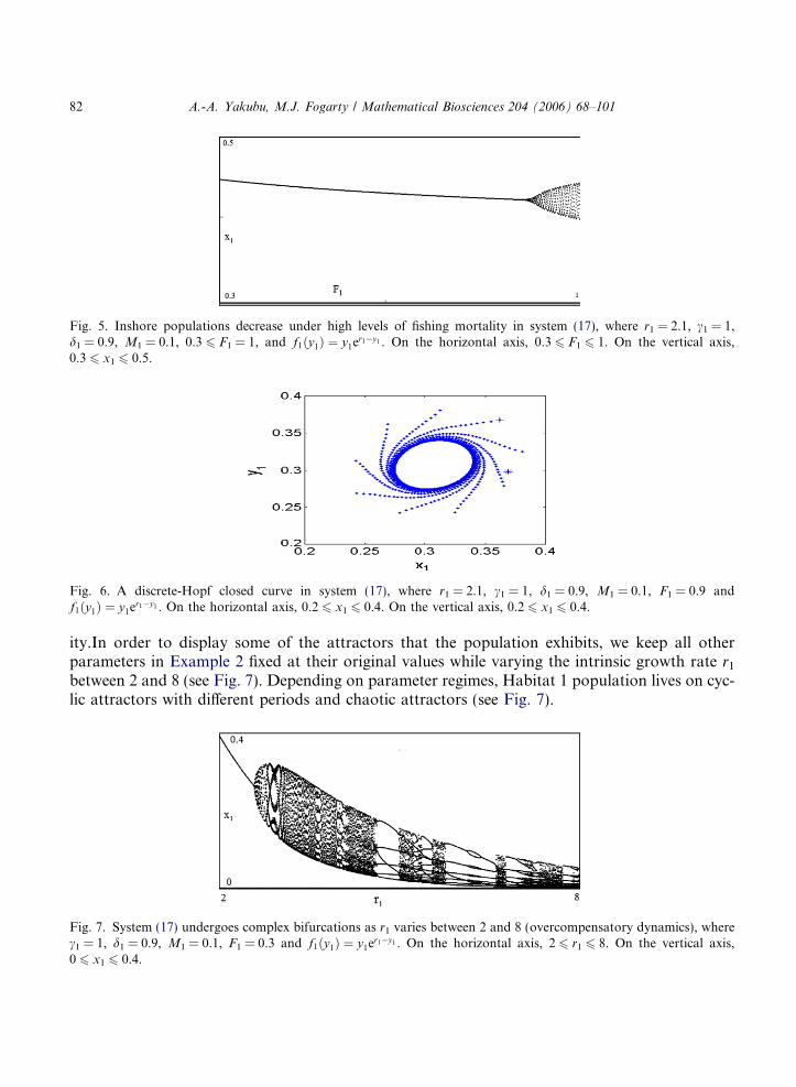
Fig. 5. Inshore populations decrease under high levels of fishing mortality in system (17), where r1 = 2.1, c1 = 1,d1 = 0.9, M1 = 0.1, 0.3 6 F1 = 1, and f1ðy1Þ ¼ y1er1�y1 . On the horizontal axis, 0.3 6 F1 6 1. On the vertical axis,0.3 6 x1 6 0.5.

Fig. 6. A discrete-Hopf closed curve in system (17), where r1 = 2.1, c1 = 1, d1 = 0.9, M1 = 0.1, F1 = 0.9 andf1ðy1Þ ¼ y1er1�y1 . On the horizontal axis, 0.2 6 x1 6 0.4. On the vertical axis, 0.2 6 x1 6 0.4.


ity.In order to display some of the attractors that the population exhibits, we keep all otherparameters in Example 2 fixed at their original values while varying the intrinsic growth rate r1

between 2 and 8 (see Fig. 7). Depending on parameter regimes, Habitat 1 population lives on cyc-lic attractors with different periods and chaotic attractors (see Fig. 7).

Fig. 7. System (17) undergoes complex bifurcations as r1 varies between 2 and 8 (overcompensatory dynamics), wherec1 = 1, d1 = 0.9, M1 = 0.1, F1 = 0.3 and f1ðy1Þ ¼ y1er1�y1 . On the horizontal axis, 2 6 r1 6 8. On the vertical axis,0 6 x1 6 0.4.


5. Two-habitat systems without larval transport

In this section, we use model (5) to study the effects of migration, compensatory and overcom-pensatory dynamics on persistence of the species in both Habitat 1 and Habitat 2 natal regions,where there is no transport of larvae between the two habitats and c2 = 1.


In the absence of Habitat 1 population, the Habitat 2 population is on a positive fixed pointattractor whenever the prerecruits are governed by compensatory dynamics. However, in the ab-sence of the Habitat 2 population, persistence of the Habitat 1 population is determined by R1

d .When all prerecruits are governed by compensatory dynamics, then R1

d < 1 implies Habitat 1population extinction while the Habitat 2 population persists. However, R1

d > 1 implies persis-tence of both Habitats 1 and 2 populations. We collect these in the following result.

Theorem 4. In model (5), for each i 2 {1,2}, let Habitat i (pre-migration) local dynamics becompensatory, where fi is a monotone map and c2 = 1.

(a) If

R1d < 1;

then every positive solution approaches

0;1

g2ð0Þg�1

2

g2ð0ÞR2

d

! !
as t!1, and the species goes extinct in Habitat 1 while it persists on a fixed point attractor inHabitat 2.
(b) If

R1d > 1;

then every positive solution approaches

1

c1g1ð0Þg�1

1

g1ð0ÞR1

d

!;X �21

!
as t!1, and the species persists on both Habitats 1 and 2, where X �21 is the unique positive solutionof the equation
d2q2xþ 1

g2ð0Þf2ðg2ð0ÞxÞ þ ð1� d1Þq1X 11 ¼ x;

and

X 11 ¼1

c1g1ð0Þg�1

1

g1ð0ÞR1

d

!:

The Proof of Theorem 4 is in the Appendix.


In the following example, Example 4, we use compensatory dynamics via the Beverton–Holtmodel to illustrate the effects of high levels of fishing mortality and migration on the persistenceof both Habitat 1 and Habitat 2 subpopulations in Eqs. (9) and (10). That is, model (5) withc2 = 1.

Example 4. Consider model (5) with

Fig. 8wherefixed.

fiðxiÞ ¼aixi

1þ bixi

for each i 2 {1,2}, where

a1 ¼ a2 ¼ � lnð0:9Þ; a1 ¼ a2 ¼ 1:1; b1 ¼ b2 ¼ c2 ¼ 1; c1 ¼ 0:6; M1 ¼ M2 ¼ 0:1;

F 1 ¼ 0:3; and F 2 ¼ 0:3:

In Example 4, R1d ¼ 1:664, and R2

d ¼ 2:773. As predicted by Theorem 4 the Habitat 1 and Hab-itat 2 populations persist on a fixed point attractor at ðX 11;X �21Þ ¼ ð1:006; 1:864Þ. To explore theeffects of migration on the persistence of both Habitat 1 and Habitat 2 populations, we keep allother parameters in Example 4 fixed at their current values while varying the proportion of migra-tory Habitat 1 adults, (1 � d1), between 0 and 1. R1

d < 1 whenever (1 � d1) is bigger than 0.493(that is, R1

d < 1 whenever d1 is smaller than 0.507). Fig. 8 shows that, resilience of the Habitat1 population is weakened with increasing levels of migration while that of Habitat 2 populationis strengthened. However, due to density-dependence, Habitat 2 population increases to a maxi-mum before declining to its carrying capacity while Habitat 1 population goes extinct.

High level of exploitation weakens the resilience of both Habitat 1 and Habitat 2 sub-popula-tions. However, high level of Habitat 1 migration with no transport of larvae between subpopu-lations eventually results in Habitat 1 population extinction while the Habitat 2 population issustained.

. In Example 4, inshore adult migration weakens inshore population while strengthening offshore population,the proportion of migratory Habitat 1 adults, (1 � d1), is varied between 0 and 1 while all other variables are keptOn the horizontal axis, 0 6 (1 � d1) 6 1. On the vertical axis, 0 6 x1,x2 6 1.



Single-species age-structured models with no migration support multiple attractors (Example1). Also, migration linked metapopulation models are capable of supporting multiple attractorswhere the independent local populations live on single attractors. For example, in a two-habitatmetapopulation model without age-structure, Hastings [31] showed that out-of-phase (asymmet-ric) initial conditions with identical local reproduction functions (f1 = f2) can support multipleattractors with fractal basin boundaries for parameter values in the chaotic regime (overcompen-satory dynamics). In this section, we study the impact of harvesting and overcompensatorydynamics on model (5), where the local reproduction functions are identical and there is no trans-port of larvae between the habitats. We focus on situations where symmetric initial populationsizes (x1 = x2) live on either a pre-selected n-cycle or a limit cycle attractor. The pre-selected sym-metric (n-cycle) attractor can coexist with a ‘new’ asymmetric attractor (multiple attractors, seeFig. 9). All positive symmetric initial conditions as well as some positive asymmetric ones areattracted to the pre-selected attractor. Lemma 4 implies that, for some survival and migrationrates, Habitats 1 and 2 population dynamics are equivalent whenever the underlying local repro-duction functions are scalar multiples of each other.

Lemma 4. In model (5), if

Fig. 9cycle

c1g1ðc1g1ð0Þx1Þ ¼ g2ðg2ð0Þx1Þ; c2 ¼ 1 and d2q2 þ ð1� 2d1Þq1 ¼ 0;

then the set of symmetric initial conditions,

D � fx ¼ ðx1; x2Þ 2 R2þjx1 ¼ x2g

is invariant and the Habitat 2 dynamics are qualitatively equivalent to the Habitat 1 dynamics.

Proof. Since c2 = 1, model (5) reduces to Eqs. (9) and (10). To establish the result, we use the twoequations to show that x1(t + 1) = x2(t + 1) whenever x1(t) = x2(t) and x1(t � 1) = x2(t � 1).Notice that c1g1(c1g1(0)x1(t � 1)) = g2(g2(0)x1(t � 1)) implies c1x1(t � 1)g1(c1g1(0)x1(t � 1)) =

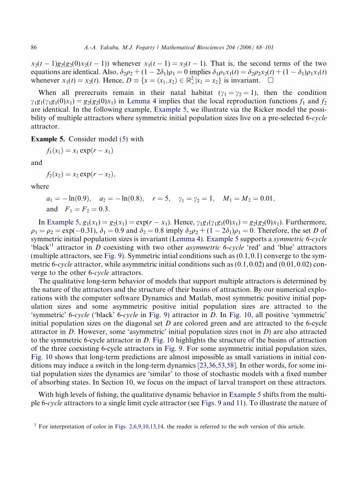
. In Example 5, a 6-cycle attractor in the set D of symmetric initial population sizes coexisting with two other 6-attractors in the set of asymmetric initial population sizes.


x2(t � 1)g2(g2(0)x2(t � 1)) whenever x1(t � 1) = x2(t � 1). That is, the second terms of the twoequations are identical. Also, d2q2 + (1 � 2d1)q1 = 0 implies d1q1x1(t) = d2q2x2(t) + (1 � d1)q1x1(t)whenever x1(t) = x2(t). Hence, D � fx ¼ ðx1; x2Þ 2 R2

þjx1 ¼ x2g is invariant. h

When all prerecruits remain in their natal habitat (c1 = c2 = 1), then the conditionc1g1(c1g1(0)x1) = g2(g2(0)x1) in Lemma 4 implies that the local reproduction functions f1 and f2

are identical. In the following example, Example 5, we illustrate via the Ricker model the possi-bility of multiple attractors where symmetric initial population sizes live on a pre-selected 6-cycleattractor.


1 Fo

f1ðx1Þ ¼ x1 expðr � x1Þ
and
f2ðx2Þ ¼ x2 expðr � x2Þ;
where
a1 ¼ � lnð0:9Þ; a2 ¼ � lnð0:8Þ; r ¼ 5; c1 ¼ c2 ¼ 1; M1 ¼ M2 ¼ 0:01;

and F 1 ¼ F 2 ¼ 0:3:

In Example 5, g1(x1) = g2(x1) = exp(r � x1). Hence, c1g1(c1g1(0)x1) = g2(g2(0)x1). Furthermore,q1 = q2 = exp(�0.31), d1 = 0.9 and d2 = 0.8 imply d2q2 + (1 � 2d1)q1 = 0. Therefore, the set D ofsymmetric initial population sizes is invariant (Lemma 4). Example 5 supports a symmetric 6-cycle‘black’1 attractor in D coexisting with two other asymmetric 6-cycle ‘red’ and ‘blue’ attractors(multiple attractors, see Fig. 9). Symmetric intial conditions such as (0.1,0.1) converge to the sym-metric 6-cycle attractor, while asymmetric initial conditions such as (0.1,0.02) and (0.01,0.02) con-verge to the other 6-cycle attractors.

The qualitative long-term behavior of models that support multiple attractors is determined bythe nature of the attractors and the structure of their basins of attraction. By our numerical explo-rations with the computer software Dynamics and Matlab, most symmetric positive initial pop-ulation sizes and some asymmetric positive initial population sizes are attracted to the‘symmetric’ 6-cycle (‘black’ 6-cycle in Fig. 9) attractor in D. In Fig. 10, all positive ‘symmetric’initial population sizes on the diagonal set D are colored green and are attracted to the 6-cycleattractor in D. However, some ‘asymmetric’ initial population sizes (not in D) are also attractedto the symmetric 6-cycle attractor in D. Fig. 10 highlights the structure of the basins of attractionof the three coexisting 6-cycle attractors in Fig. 9. For some asymmetric initial population sizes,Fig. 10 shows that long-term predictions are almost impossible as small variations in initial con-ditions may induce a switch in the long-term dynamics [23,36,53,58]. In other words, for some ini-tial population sizes the dynamics are ‘similar’ to those of stochastic models with a fixed numberof absorbing states. In Section 10, we focus on the impact of larval transport on these attractors.

With high levels of fishing, the qualitative dynamic behavior in Example 5 shifts from the multi-ple 6-cycle attractors to a single limit cycle attractor (see Figs. 9 and 11). To illustrate the nature of

r interpretation of color in Figs. 2,6,9,10,13,14, the reader is referred to the web version of this article.

Fig. 10. Basins of attraction of three 6-cycle attractors in Example 5. The region along the diagonal includes a subset ofthe basin of attraction of the attractor in the set D of symmetric initial population sizes, while the other two regionscontain the basins of attraction of the two asymmetric attractors in Fig. 9. On the horizontal axis, 0 6 x1 6 0.2. On thevertical axis, 0 6 x1 6 0.2.

Fig. 11. A limit cycle attractor in the set of asymmetric initial population sizes, where all parameters are fixed at theircurrent values in Example 5 and F1 = F2 = 0.38. On the horizontal axis, 0 6 x1 6 0.2. On the vertical axis, 0 6 x2 6 0.2.


this bifurcation and the importance of fishing on species resilience, we keep all parameters fixed attheir current values in Example 5 while the identical Habitat 1 and Habitat 2 fishing mortalities(F1 = F2) are increased past 0.3. When F1 = F2 = 0.38, the system supports a limit cycle attractorin the set of asymmetric initial conditions (see Fig. 11). Our numerical explorations show thatmost positive initial population sizes are attracted to the limit cycle attractor.

Two-habitat population models without larval exchange between the subpopulations are capa-ble of supporting multiple attractors with complicated basins of attraction, where larval popula-tions are governed by identical overcompensatory dynamics. However, fishing pressure can alter


such systems from multiple n-cycle attractors with complicated basins of attraction to single limitcycle attractors with simpler basins of attraction. In other words, high levels of fishing give rise todrastically different aggregate dynamics of the full system and these results may have seriousimplications for conservation, ecology and evolutionary biology of the species.

6. Two-habitat systems with larval transport

The qualitative dynamics of model (4) can change dramatically through larval dispersal. In thissection, we use compensatory and overcompensatory mechanisms in the model to highlight theimportance of larval subsidies to heavily exploited Habitat 1 population. In particular, we usethe threshold parameters,

R1d and R2

d

from Eqs. (13) and (15) to show that it is possible to sustain high level of fishing in the Habitat 1population if exploitation rates are low in Habitat 2 population (Example 6).


When all prerecruits are governed by compensatory dynamics and all Habitat 1 adults are sed-entary, then R1

d < 1 and R2d < 1 imply Habitat 1 and Habitat 2 population extinction where there

is larval exchange from Habitat 2 to Habitat 1 group. However, R2d > 1 implies persistence of

both Habitats 1 and 2 populations. We collect these in the following result.

Theorem 5. In model (5), for each i 2 {1,2}, let Habitat i (pre-migration) local dynamics becompensatory, where fi is a monotone map and d1 = 1.

(a) If R1d < 1 and R2

d < 1 then every solution approaches the origin as t!1, and the species goesextinct in both Habitats 1 and 2.

(b) If R1d < 1 and R2

d < 1 then every positive solution approaches

1

c1g1ð0Þg�1

1

g1ð0ÞR1

d

!; 0

!

as t!1, and the species persists in Habitat 1 while it goes extinct in Habitat 2.(c) If R2

d > 1 and c1g1((1 � c2)g2(0)X21) > 1, then the species persists in both Habitats 1 and 2where

X 21 ¼ g�12

g2ð0ÞR2

d

!:

The Proof of Theorem 5 is in the Appendix.

In the following example, Example 6, we use the Beverton–Holt model in model (4) to illustratethe qualitative differences that emerge in comparison of migration and larval transport linkedindependent Habitat 1 and Habitat 2 groups.



Fig. 1valuesF2 = 2horizo

f1ðx1Þ ¼a1x1

1þ b1x1

and

f2ðx2Þ ¼a2x2

1þ b2x2

;

where

a1 ¼ a2 ¼ 1:1; b1 ¼ b2 ¼ c2 ¼ 1; a1 ¼ F 2 ¼ 0; a2 ¼ � lnð0:9Þ;c1 ¼ 0:9; M1 ¼ M2 ¼ 0:1; and F 1 ¼ 4:7:

In Example 6, Habitat 1 is a heavily exploited region with R1d ¼ 0:998 < 1 while Habitat 2 is a

no-take region with R2d ¼ 5:925 > 1. Without larval exchange (c2 = 1), Habitat 1 population goes

extinct while Habitat 2 population persists and the system supports a stable equilibrium popula-tion at (X11,X21) = (0,4.477) (Theorem 2). That is, Example 6 is a sink-source system. With lar-val exchange and low to moderate Habitat 2 fishing, Habitat 1 population recovers fromextinction and both Habitats 1 and 2 populations persist whenever R2

d > 1 (Theorem 5).

To study the impact of different fishing pressures in Habitat 2 on the Habitat 1 population, wekeep all the parameters fixed at their current values in Example 6 while varying the proportion ofprerecruits that do not remain in Habitat 2, (1 � c2), between 0 and 1 (see Fig. 12). The five graphsin Fig. 12 show that, Habitat 1 population is largest under low to moderate fishing pressures cou-pled with low to moderate levels of larval transport from Habitat 2 to Habitat 1. In all five cases,low to moderate exploitation of Habitat 2 population coupled with low to moderate levels of lar-val transport saves Habitat 1 population from extinction (see Fig. 12). The five graphs of Fig. 12highlight the resilience of inshore lobsters under different fishing pressures on the offshore lobsterpopulation.

2. Resilience of Habitat 1 population under five different fishing mortalities in Habitat 2. Under low to moderateof larval transport, Habitat 1 population is largest when F2 = 0, followed by F2 = 0.3, F2 = 0.5, F2 = 1 and

. In all five cases, Habitat 1 population crashes when larval transport from Habitat 2 to 1 is very high. On thental axis, 0 < 1 � c2 < 1. On the vertical axis, 0 6 x1 6 0.9.



Linked subpopulations under overcompensatory mechanisms are capable of generating multi-ple attractors with complicated basins of attraction (see Example 5 and [5–7,31,58]). In this sec-tion, we use Example 5 to study the impact of larval exchange on coexisting attractors and theirbasin structures. We illustrate that larval transport can shift the qualitative behavior of systemsfrom multiple attractors with fractal basin boundaries to single attractors with simpler basinsof attraction. That is, it is possible to make accurate long-term prediction of stability and resil-ience of species in systems with larval transport where such predictions are impossible without lar-val transport.


Fig. 1transpattracdiffereaxis, 0

f1ðx1Þ ¼ x1 expðr � x1Þ
and
f2ðx2Þ ¼ x2 expðr � x2Þ;

where

a1 ¼ � lnð0:9Þ; a2 ¼ � lnð0:8Þ; r ¼ 5; c1 ¼ 1;

M1 ¼ M2 ¼ 0:01; F 1 ¼ F 2 ¼ 0:3: and vary c2 between 0 and 1:

When there is no transport of larvae between the subpopulations, c2 = 1 and Example 7reduces to Example 5 (see Figs. 9 and 10). In Example 7, we study the impact of varying c2

or (1 � c2) between 0 and 1 on the dynamics in Example 5 while keeping all the other param-eters fixed at their current values in Example 5 or 7. With low levels of larval exchange from

3. As in Example 5, Example 7 supports multiple attractors with complicated basins of attraction when larvalort is low. In particular, when (1 � c2) = 0.01, Example 7 supports a 6-cycle attractor coexisting with a limit cycletor. Most positive initial conditions are attracted to the limit cycle attractor. The different colors illustrate thent long-term outcome of the different initial conditions. On the horizontal axis, 0 6 x1 6 0.15. On the vertical6 x2 6 0.15.

Fig. 14. Example 7 only supports one limit cycle attractor when (1 � c2) = 0.3. Most positive initial conditions areattracted to the limit cycle attractor. The different colors illustrate the long-term outcome of the different initialconditions. On the horizontal axis, 0 6 x1 6 0.15. On the vertical axis, 0 6 x2 6 0.15.


Habitat 2 to Habitat 1 group, Example 7 (like Example 5) supports multiple extractors withvery thin basins of attraction. In particular, when c2 = 0.99 and (1 � c2) = 0.01 in Example 7,the system supports two coexisting attractors, a 6-cycle and a limit cycle attractors. By ournumerical explorations, the limit cycle is the long-term outcome of most initial population sizes(see Fig. 13).

By our numerical explorations, at moderate to high levels of larval exchange, Example 7 sup-ports only a single attractor with fat basin of attraction. In particular, when c2 = 0.7 and(1 � c2) = 0.3 in Example 7, the system supports only one attractor, a limit cycle (seeFig. 14). The number of attractors and structure of attractor-basins is a complicated functionof the larval exchange rate c2 and the natal region dynamics.

7. Conclusion

Doebeli, Hastings, Levin and others have studied the impact of intraspecific competition onlife-history dynamics in metapopulation models with no age-structure [10,11,31,40–42,44–46].This article focuses on using a two-habitat metapopulation model with age-structure to expandthe conclusions of Fogarty on inshore–offshore lobster systems with larval interchange and direc-ted movement of adults to include metapopulation models with isolated habitats under compen-satory (monotone) and overcompensatory (oscillatory) dynamics. We use mathematical andsimulation results to investigate the influence of various assumptions (such as whether the dynam-ics of the isolated habitats are compensatory or overcompensatory; fishing levels, migration levels,and survival rates) on the dynamics of population models linking subpopulations through larvaltransport and directed movement of adults. The results of Fogarty predict that low levels of larvalsubsidy from offshore to inshore populations could contribute strongly to the resilience of inshorepopulations to high levels of exploitation in coastal areas, where larvae populations are governedby the Beverton–Holt model [16]. Our results support this prediction in two-habitat systems with


larval transport and directed movements of adults, where larval population dynamics are eithercompensatory or overcompensatory. That is, conservative management of larval source popula-tions could contribute to the resilience of exploited species.

Using metapopulation models with no age-structure, Hastings, Levin, Yakubu and Castillo-Chavez proved that compensatory dynamics on local populations leads to a stable equilibriumat the metapopulation level [10,11,31,40]. Similarly, metapopulation models with larval transportsupport a stable equilibrium population whenever the larvae populations are under compensatorydynamics and the threshold parameters Ri

d are bigger than 1. However, the stable equilibriumpopulation decreases in size with increasing levels of fishing.

In 1999, Hastings and Botsford [33] demonstrated that for a delay-difference model with sed-entary adults and implicit dispersal of progeny, marine reserves can provide protection equivalentto other fishery management tools such as reductions in exploitation rates while providing sub-stantial resilience. These results complement the findings of our analysis.

Single patch age-structured models as well as metapopulation models with no age-struc-ture are capable of supporting multiple attractors with complex basin structures. The inter-actions of age structure, directed movements of adults, larval transport, fishing pressure andovercompensatory dynamics has helped our understanding of the role that initial populationsizes play on the life-history dynamics of a metapopulation. As the complexity of the larvaldynamics increases the overall fate of a metapopulation becomes less predictable to the pointthat it may be impossible to determine, with any degree of certainty, the fate of such meta-population. In other words, fractal basins of attraction generated by the interactionsbetween age-structure, directed movements of adults, larval transport, fishing pressure andovercompensatory dynamics bring a large degree of uncertainty to the notion of predictionin deterministic metapopulation models. Depending on model parameters, increasing larvaltransport or fishing pressure can shift the system dynamics from multiple attractors withcomplicated attractor basins (unpredictable) to a single attractor with simple attractor basin(predictable).

Acknowledgments

The authors thank the referees for useful comments, corrections and suggestions. We alsothank Dr. Ambrose Jearld for his support throughout this study. This research has been partiallysupported by the National Marine Fisheries Service, Northeast Fisheries Science Center (WoodsHole, MA 02543).

Appendix

We use the following general result of Kulenovic and Yakubu [39], Theorem A.1, to proveTheorem 1. To state the result, we first introduce the following notation. Let

h : ½0;1Þ� ½0;1Þ ! ½0;1Þ


be a continuous function, where x1 2 [0,1) is the fixed point of the difference equation

xðt þ 1Þ ¼ hðxðtÞ; xðt � 1ÞÞ; t ¼ 0; 1; 2; . . . ðA:1Þ
That is,
X1 ¼ hðX1;X1Þ:

Theorem A.1 [39]. Assume that

h : ½0;1Þ � ½0;1Þ ! ½0;1Þ
satisfies the following properties:
1. There exist two numbers L and U, 0 < L < U such that

hðL; LÞP L; hðU ;UÞ 6 U

and h(x,y) is non-decreasing in x and y in the closed interval [L,U].2. The equation

hðx; xÞ ¼ x

has a unique positive solution X1 in [L,U].

Then system (A.1) has the unique positive fixed point X1 in [L,U], and every positive initialcondition in [L,U] converges to it.

Proof of Theorem 1. The positive fixed point of Eq. (11), X21 is the solution of the equation

d2q2 þ g2ðX 21g2ð0ÞÞ ¼ 1:

That is,

1� d2q2 � g2ðX 21g2ð0ÞÞ ¼ 0;

where X 21 ¼g�1

2ð1�d2q2Þg2ð0Þ

. Let

HðxÞ ¼ 1� d2q2 � g2ðxg2ð0ÞÞ:

Since gið0Þ > 1; d2q2 < 1; g0i < 0 and limxi!1giðxiÞ ¼ 0,

Hð0Þ ¼ 1� d2q2 � g2ð0Þ < 0; limx!1

HðxÞ > 0 and H 0ðxÞ > 0 for all x P 0:

Next, we find L > 0 satisfying h(L,L) P L, where

hðx; yÞ ¼ d2q2xþ 1

g2ð0Þf2ðyg2ð0ÞÞ;

and the monotone map f2(y) = yg2(y). Notice that h(x,y) is non-decreasing in x and y.By a simple calculation, we obtain that

hðL; LÞ � L ¼ �LHðLÞ:


Consequently, h(L,L) � L > 0 if and only if H(L) < 0. That is, h(L,L) � L > 0 if and only ifL < X21. Proceeding exactly as above, we find U > X21 satisfying h(U,U) � U 6 0.

Choose arbitrary initial population sizes x2(�1) > 0 and x2(0) > 0 (Lemma 2). Now, choose Land U such that

0 < L < minfx2ð�1Þ; x2ð0Þ;X 21g and U > maxfx2ð�1Þ; x2ð0Þ;X 21g:
Then the solution {x2(t)} stays in the interval [L,U] for all t P 0, and by Theorem A.1 convergesto the unique positive fixed point. h
Proof of Lemma 3

x2ðt þ 1Þ ¼ d2q2x2ðtÞ þ x2ðt � 1Þg2ðg2ð0Þx2ðt � 1ÞÞ
implies that for each t 2 {0,1,2, . . .}
x2ðt þ 1ÞP x2ðt � 1Þg2ðg2ð0Þx2ðt � 1ÞÞ:
By the difference inequalities in [37], for each t 2 {0,1,2, . . .}
x2ðt þ 1ÞP u2ðtÞ;
where the sequence {u2(t)} satisfies the corresponding difference equation
u2ðtÞ ¼ u2ðt � 1Þg2ðg2ð0Þu2ðt � 1ÞÞ; ðA:2Þ
where u2(�1) = x2(�1). Without loss of generality, we assume that x2(�1) > 0 (Lemma 2).
The set of density sequences generated by Eq. (A.2) is equivalent to the set of iterates of themap f2ðu2Þ ¼ 1

g2ð0Þf2ðg2ð0Þu2Þ. The positive fixed point of f 2 is bX 2 ¼ X 2

g2ð0Þ, where X2 is the positive

fixed point of f2(u2) = u2g2(u2). Moreover, f 2ðu2Þ > u2 whenever 0 < u2 < bX 2 and f2(u2) < u2

whenever u2 > bX 2. Consequently, I2 ¼ f 2ð½0; bX 2�Þ is a global attractor for the continuous

function f 2. Let �I2 � f 2ð½bX 2;max I2�Þ. Then, min�I2 > 0 and the closed f 2-invariant interval½min�I2;max I2� is either a trapping region that traps all positive initial population sizes or a globalattractor in (0,1). Therefore, every solution of Eq. (A.2) satisfies

limt!1

inf u2ðtÞ > 0

whenever u2(�1) > 0. These imply that

limt!1

inf x2ðtÞ > 0

whenever x2(�1) > 0 or x2(0) > 0. h

Proof of Theorem 2

x1ðt þ 1Þ ¼ d1q1x1ðtÞ þ c1x1ðt � 1Þg1ðc1g1ð0Þx1ðt � 1ÞÞ
implies that for each t 2 {0,1,2, . . .},
x1ðt þ 1Þ 6 d1q1x1ðtÞ þ c1g1ð0Þx1ðt � 1Þ:
(a) By the difference inequalities in [37], for each t 2 {0,1,2, . . .}
x1ðtÞ 6 u1ðtÞ;



u1ðt þ 1Þ ¼ d1q1u1ðtÞ þ c1g1ð0Þu1ðt � 1Þ; ðA:3Þ
where u1(�1) = x1(�1) and u1(0) = x1(0).
R1d < 1 implies that (d1q1 + c1g1(0)) < 1, and every solution of Eq. (A.3) satisfies

limt!1

uðtÞ ¼ 0 ½37�:

These imply that

limt!1

x1ðtÞ ¼ 0

for every solution of model (7) whenever R1d < 1. Hence, the zero fixed point is globally asymp-

totically stable whenever R1d < 1.

(b) The positive fixed point of Eq. (9), X11 is the unique positive solution of the equation

d1q1 þ c1g1ðc1g1ð0ÞX 11Þ ¼ 1:

That is,

1� d1q1 � c1g1ðc1g1ð0ÞX 11Þ ¼ 0

and

X 11 ¼1

c1g1ð0Þg�1

1

1� d1q1

c1

� �¼ 1

c1g1ð0Þg�1

1

g1ð0ÞR1

d

!:

Let

HðxÞ ¼ 1� d1q1 � c1g1ðc1g1ð0ÞxÞ:
R1
d > 1 implies that d1q1 + c1g1(0) > 1,

Hð0Þ ¼ 1� d1q1 � c1g1ð0Þ < 0; limx!1

HðxÞ > 0 and H 0ðxÞ > 0 for all x P 0:



g1ð0Þf1ðc1g1ð0ÞyÞ;

and the monotone map f1(c1g1(0)y) = c1g1(0)yg1(c1g1(0)y). With our assumptions, h(x,y) is non-decreasing in x and y.

By a simple calculation, we obtain that

hðL; LÞ � L ¼ �LHðLÞ:
Consequently, h(L,L) � L > 0 if and only if H(L) < 0. That is, h(L,L) � L > 0 if and only ifL < X11. Proceeding exactly as above, we find U > X11 satisfying h(U,U) � U 6 0.
Choose arbitrary initial population sizes x1(�1) > 0 and x1(0) > 0. Now, choose L and U suchthat

0 < L < minfx1ð�1Þ; x1ð0Þ;X 11g and U > maxfx1ð�1Þ; x1ð0Þ;X 11g:
Then the solution {x1(t)} stays in the interval [L,U] for all t P 0, and by Theorem A.1 convergesto the unique positive fixed point. h


Proof of Theorem 3. (a) When R1d < 1 proceed exactly as in the Proof of Theorem 2(a) to establish

the result.(b) As shown by a standard linearization argument, R1

d > 1 implies that the origin is unstable.That is, all sufficiently small positive initial conditions go away from zero under iterations.

x1ðt þ 1Þ ¼ d1q1x1ðtÞ þ c1x1ðt � 1Þg1ðc1g1ð0Þx1ðt � 1ÞÞ

implies that for each t 2 {0,1,2, . . .}

x1ðt þ 1ÞP c1x1ðt � 1Þg1ðc1g1ð0Þx1ðt � 1ÞÞ:

By the difference inequalities in [37], for each t 2 {0,1, 2,. . .}



u1ðtÞ ¼ c1u1ðt � 1Þg1ðc1g1ð0Þu1ðt � 1ÞÞ; ðA:4Þ

where u1(�1) = x1(�1). Without loss of generality, we assume that x1(�1) > 0 (Lemma 2).The set of density sequences generated by Eq. (A.4) is equivalent to the set of iterates of the

map f 1ðu1Þ ¼ 1g1ð0Þ

f1ðc1g1ð0Þu1Þ ¼ c1u1g1ðc1g1ð0Þu1Þ. If c1g1(0) > 1, then we proceed as in the

Proof of Lemma 3. That is, the monotone map f 1 has a positive fixed point, denoted by bX 1, andthe origin is unstable. Furthermore, f 1ðu1Þ > u1 whenever 0 < u1 < bX 1 and f1(u1) < u1 whenever

u1 > bX 1. Consequently, I1 � f 1ð½0; bX 1�Þ is a global attractor for the continuous function f 1. LetJ1 � f 1ð½bX 1;max I1�Þ. Then, min I1 > 0 and the closed f 1-invariant interval ½min J1;max I1� iseither a trapping region that traps all positive initial population sizes or a global attractor in(0,1). Therefore, every solution of Eq. (A.4) satisfies

limt!1

inf u1ðtÞ > 0

whenever u1(�1) > 0. These imply that

limt!1

inf x1ðtÞ > 0

whenever x1(�1) > 0 or x1(0) > 0.By Lemma 3, x1(t) > 0 for all t P 1 whenever either x1(0) > 0 or x1(�1) > 0. Thus,

limt!1

inf x1ðtÞ > 0

whenever c1g1(0) > 1, and either x1(0) > 0 or x1(�1) > 0.Now, we consider the case c1g1(0) < 1. R1

d > 1 implies that d1q1 + c1g1(0) > 1. Now, choose0 < �, h < 1 so that d1q1 + c1 g1(c1g1(0)x1) > 1 + h whenever 0 < x1 6 �. Consequently, if x1(t) 6 �for each t 2 {0,1,2, . . .}, then

x1ðt þ 1Þ ¼ d1q1x1ðtÞ þ c1x1ðt � 1Þg1ðc1g1ð0Þx1ðt � 1ÞÞP d1q1x1ðtÞ þ ð1þ h� d1q1Þx1ðt � 1Þ:


x1ðtÞP u1ðtÞ;



u1ðt þ 1Þ ¼ d1q1u1ðtÞ þ ð1þ h� d1q1Þu1ðt � 1Þ; ðA:5Þ

where u1(�1) = x1(�1) and u1(0) = x1(0).Since d1q1 + (1 + h � d1q1) > 1, every solution of Eq. (A.5) satisfies

limt!1

inf x1ðtÞ > 0 ½37�

whenever either u1(0) > 0 or u1(�1) > 0. Thus,

limt!1

inf x1ðtÞ > 0

whenever either x1(0) > 0 or x1(�1) > 0. This completes the proof. h

The Proof of Theorem 4 uses a ‘Limiting Theorem’ from [5]. To state the result, consider thefollowing general discrete-time system:

yðt þ 1Þ ¼ F ðyðtÞÞ; yð0Þ ¼ y 2 Rmþ;

zðt þ 1Þ ¼ GðyðtÞ; zðtÞÞ; zð0Þ ¼ z 2 Rkþ;

�ðA:6Þ

where F and G are continuous functions. We make the following three assumptions in system(A.6): solutions of system (A.6) remain non-negative and are bounded if initial values are non-negative, System y(t + 1) = F(y(t)) admits a globally attracting fixed point Y1 in Rm

þ, andz(t + 1) = G(Y1,z(t)) admits a globally asymptotically stable fixed point Z1 in Rk

þ.

Theorem A.2 [5]. (Y1,Z1) is a globally attracting fixed point of system (A.6) in Rmþkþ .

Proof of Theorem 4. To apply Theorem A.2, define

F : ½0;1Þ � ½0;1Þ ! ½0;1Þ� ½0;1Þ
by
F ðx1; y1Þ ¼ ðd1q1x1 þ c1y1g1ðc1g1ð0Þy1Þ; x1Þ:
The set of iterates of F is equivalent to the set of density sequences generated by Eq. (9). By The-orem 2, F admits a globally attracting fixed point Y1 = (0,0) whenever R1
d < 1 whileY1 = (X11,X11) whenever R1

d > 1.When R1

d < 1, define

G : f0g � ½0;1Þ� f0g � 0;1½ Þ ! f0g � ½0;1Þ� f0g � ½0;1Þ
by
Gð0; x2; 0; y2Þ ¼ ð0; d2q2x2 þ y2g2ðg2ð0Þy2Þ; 0; x2Þ:
The set of iterates of G is equivalent to the set of density sequences generated by model (5) wherec2 = 1 and x1 � 0 (that is, Eq. (11)).
By Theorem 1, G(0,x2,0,y2) admits a globally attracting positive fixed point. Hence, TheoremA.2 implies that when R1

d < 1, then (0,X21, 0,X21) is a globally attracting fixed point of model (5)when c2 = 1.


When R1d > 1, define

G : ½0;1Þ � ½0;1Þ ! ½0;1Þ� ½0;1Þ
by
GðX 11; x2;X 11; y2Þ ¼ ðd2q2x2 þ y2g2ðg2ð0Þy2Þ þ ð1� d1Þq1X 11; x2Þ:
The set of iterates of G is equivalent to the set of density sequences generated by model (5)
restricted to the (x2,y2)-plane, where ðx1; y1Þ � ðX 11;X 11Þ; X 11 ¼ 1c1g1ð0Þ

g�11

g1ð0ÞR1

d

� �and c2 = 1.

The positive fixed point of G; ðX �21;X �21Þ, is the solution of

GðX 11; x2;X 11; y2Þ ¼ ðx2; y2Þ:
That is, X �21 is the unique positive solution of the equation
d2q2 þ g2ðg2ð0Þx2Þ þð1� d1Þq1X 11

x2

¼ 1:

That is,

1� d2q2 � g2ðg2ð0Þx2Þ �ð1� d1Þq1X 11

x2

¼ 0:

Let

HðxÞ ¼ 1� d2q2 � g2ðg2ð0ÞxÞ �ð1� d1Þq1X 11

x;

limx!0þ

HðxÞ < 0; limt!1

HðxÞ > 0 and H 0ðxÞ > 0 for all x > 0:



g2ð0Þf2ðg2ð0ÞyÞ þ ð1� d1Þq1X 11;

and the monotone map f2(y) = yg2(y). Notice that h(x,y) is non-decreasing in x and y.By a simple calculation, we obtain that

hðL;LÞ � L ¼ �LHðLÞ:
Consequently, h(L,L) � L > 0 if and only if H(L) < 0. That is, h(L,L) � L > 0 if and only ifL < X �21. Proceeding exactly as above, we find U > X �21 satisfying h(U,U) � U 6 0.
Choose arbitrary initial population sizes x2(�1) > 0 and x2(0) > 0 (Lemma 2). Now, choose Land U such that

0 < L < minfx2ð�1Þ; x2ð0Þ;X �21g and U > maxfx2ð�1Þ; x2ð0Þ;X �21g:
Then the solution {x2(t)} stays in the interval [L,U] for all t P 0, and by Theorem A.1 convergesto the unique positive fixed point. Hence, Theorem A.2 implies that when R1
d > 1, thenðX 11;X �21Þ is a globally attracting fixed point of model (5), where c2 = 1. h

Proof of Theorem 5. By Theorem 1, R2d < 1 and d1 = 1 imply that x2(t)! 0 as t!1. Now,

proceed as in the Proof of Theorem 4 and use the ‘limiting theorem’, Theorem A.2, to prove(a) and (b).


Again by Theorem 1, R2d > 1 and d1 = 1 imply that x2(t)! X21 as t!1. The limiting

equation for x1 is

x1ðt þ lÞ ¼ d1q1x1ðtÞ þ c1x1ðt � 1Þg1ðc1g1ð0Þx1ðt � 1Þ þ ð1� c2Þg2ð0ÞX 21Þþ ð1� c2ÞX 21g2ðc1g1ð0Þx1ðt � 1Þ þ ð1� c2Þg2ð0ÞX 21Þ:

This implies that for each t 2 {0,1,2, . . .}

x1ðt þ 1ÞP c1x1ðt � 1Þg1ðc1g1ð0Þx1ðt � 1Þ þ ð1� c2Þg2ð0ÞX 21Þ:
u1ðtÞ ¼ c1u1ðt � 1Þg1ðc1g1ð0Þu1ðt � 1Þ þ ð1� c2Þg2ð0ÞX 21Þ; ðA:7Þ
where u1(�1) = x1(�1).
As in the Proof of Theorem 3, c1g1((1 � c2)g2(0)X21) > 1 implies that every solution of Eq.(A.7) satisfies

limt!1

inf u1ðtÞ > 0 ½37�

whenever either u1(�1) > 0 or u1(0) > 0. Thus,

limt!1

inf x1ðtÞ > 0

whenever either x1(�1) > 0 or x1(0) > 0. h

References

[1] L.J. Allen, Persistence, extinction, and critical patch number for island populations, J. Math. Biol. 24 (1987) 617.[2] V.C. Anthony, Caddy J.F. (Eds.), Proc. of the Canadian–U.S. Workshop on Status of Assessment Science for

N.W. Atlantic Lobster (Homarus americanus) Stocks. St. Andrews, N.B. Can. Tech. Rep. Fish. Aquat. Sci. 932(Oct. 24–26, 1978).

[3] M. Begon, J.L. Harper, C.R. Townsend, Ecology: Individuals Populations and Communities, Blackwell Science,1996.

[4] R.J.H. Beverton, S.J. Holt, On the dynamics of exploited fish populations, Fish. Invest. Ser. II Mar. Fish. G.B.Minist. Agric. Fish Food (1957).

[5] J. Best, C. Castillo-Chavez, A.A. Yakubu, Hierarchical competition in discrete time models with dispersal, FieldsInst. Commun. 36 (2003) 59.

[6] C. Castillo-Chavez, A.A. Yakubu, Dispersal disease and life-history evolution, Math. Biosci. 173 (2001) 35.[7] C. Castillo-Chavez, A.A. Yakubu, Intraspecific competition dispersal and disease dynamics in discrete-time patchy

environments, in: Carlos Castillo-Chavez, Sally Blower, Pauline van den Driessche, Denise Kirschner, Abdul-AzizYakubu (Eds.), Mathematical Approaches For Emerging and Reemerging Infectious Diseases: An Introduction toModels, Methods and Theory, Springer, New York, 2002.

[8] J.S. Cobb, D. Wang, D.B. Campbell, P. Rooney, Speed and direction of swimming by postlarvae of the Americanlobster, Trans. Am. Fish. Soc. 118 (1989) 82.

[9] D. Cohen, S.A. Levin, The interaction between dispersal and dormancy strategies in varying and heterogeneousenvironments, in: E. Teramoto, M. Yamaguti (Eds.), Mathematical Topics in Population Biology, Morphogenesisand Neurosciences, Proc. Kyoto 1985, Springer, Berlin, 1987, p. 110.


[10] M. Doebeli, Dispersal and dynamics, Theor. Popul. Biol. 47 (1995) 82.[11] M. Doebeli, G.D. Ruxton, Evolution of dispersal rates in metapopulation model: branching and cyclic dynamics in

phenotype space, Evolution 5 (6) (1997) 1730.[12] D.J. Earn, S.A. Levin, P. Rohani, Coherence and conservation, Science 290 (November) (2000) 17.[13] P.L. Errington, Some contributions of a fifteen year local study of the northern bobwhite to a knowledge of

population phenomena, Ecol. Monogr. 15 (1945) 1.[14] M.J. Fogarty, Distribution and relative abundance of American lobster Homarus americanus larvae: a review,

NOAA Tech. Rep. SSRF 775 (1983) 3.[15] M.J. Fogarty, Fisheries, populations, and management, in: J. Factor (Ed.), The Biology of the American lobster,

Homarus americanus, Academic Press, New York, NY, 1995.[16] M.J. Fogarty, Implications of migration and larval interchange in American lobster (Homarus americanus)

stocks: spatial structure and resilience, in: G.S. Jamieson, A. Campbell (Eds.), Proc. of North PacificSymposium on Invertebrate Stock Assessment and Management, Can. Spec. Publ. Fish. Aquat. Sci. 125 (1998)273.

[17] M.J. Fogarty, J.S. Idoine, Recruitment dynamics in an American lobster (Homarus americanus) population, Can. J.Fish. Aquat. Sci. 43 (1986) 2368.

[18] M.J. Fogarty, D.V.D. Borden, H.J. Russell, Movements of tagged American lobster, Homarus americanus, offRhode Island, Fish. Bull. (US) 78 (1980) 771.

[19] M.J. Fogarty, L.W. Botsford, Metapopulation dynamics of marine decapods, in: P. Sale, J. Kritzer (Eds.), MarineMetapopulations (2006) 271.

[20] J.E. Franke, A.-A. Yakubu, Extinction and persistence of species in discrete competitive systems with a safe refuge,J. Math. Anal. Appl. 23 (1996) 746.

[21] M. Gadgil, Dispersal: population consequences and evolution, Ecology 52 (1971) 253.[22] J.L. Gonzalez-Andujar, J.N. Perry, Chaos, metapopulations and dispersal, Ecol. Model 65 (1993) 255.[23] C. Grebogi, E. Ott, J.A. Yorke, Chaos, strange attractors, and fractal basin boundaries in nonlinear dynamics,

Science 228 (1987) 632.[24] M. Gyllenberg, G. Soderbacka, S. Ericsson, Does migration stabilize local population dynamics? Analysis of a

discrete metapopulation model, Math. Biosci. 118 (1993) 25.[25] I. Hanski, Metapopulation Ecology, Oxford University, Oxford, 1999.[26] I. Hanski, Single-species metapopulation dynamics-concepts, models and observations, Biol. J. Linn. Soc. 42

(1991) 17.[27] I. Hanski, M.E. Gilpin, Metapopulation Biology: Ecology, Genetics, and Evolution, Academic Press, San Diego,

CA, 1997.[28] I. Hanski, D. Simberloff, The metapopulation approach, its history, conceptual domain and application

to conservation, in: I. Hanski, M. Gilpin (Eds.), Metapopulation Biology, Academic Press, San Diego, 1997, p. 5.[29] M.P. Hassell, The Dynamics of Competition and Predation, Studies in Biol, vol. 72, The Camelot, 1976.[30] M.P. Hassell, J.H. Lawton, R.M. May, Patterns of dynamical behavior in single species populations, J. Anim.

Ecol. 45 (1976) 471.[31] A. Hastings, Complex interactions between dispersal and dynamics: lessons from coupled logistic equations,

Ecology 75 (1993) 1362.[32] A. Hastings, Dynamics of a single species in a spatially varying environment: the stabilizing role of high dispersal

rates, J. Math. Biol. 16 (1982) 49.[33] A. Hastings, L.W. Botsford, Equivalence in yield from marine reserves and traditional fisheries management,

Science 284 (1999) 1537.[34] S.M. Henson, J.M. Gushing, Hierarchical models of intraspecific competition: scramble versus contest, J. Math.

Biol. 34 (1996) 755.[35] D.S. Holland, R.J. Brazee, Marine reserves for fisheries management, Mar. Res. Econ. 11 (1996) 157.[36] I. Kan, Open sets of diffeomorphisms having two attractors, each with an everywhere dense basin, Bull. AMS 31 (1)

(1994) 68.[37] V.L. Kocic, G. Ladas, Global Behavior of Nonlinear Difference Equations of Higher Order with Applications,

Kluwer Academic, Dordrecht, 1993.


[38] J.P. Kritzer, P.F. Sale, Metapopulation ecology in the sea: from Levin’s model to marine ecology and fisheriesscience, Fish Fisheries 5 (2004) 131.

[39] M. Kulenovic, A.-A. Yakubu, Compensatory versus overcompensatory dynamics in density-dependent Lesliemodels, J. Differ. Equat. Appl. 10 (13–15) (2004) 1251.

[40] S.A. Levin, Dispersion and population interactions, Am. Nat. 108 (1974) 207.[41] S.A. Levin, The problem of pattern and scale in ecology, Ecology 73 (1992) 1943.[42] S. Levin, R.T. Paine, Disturbance, patch formation, and community structure, Proc. Natl. Acad. Sci. USA 68

(1974) 2744.[43] R. Levins, Extinction, Lect. Notes Math. 2 (1970) 75.[44] R. Levins, Some demographic and genetic consequences of environmental heterogeneity for biological control,

Bull. Entomol. Soc. Am. 15 (1969) 237.[45] R. Levins, The effect of random variation of different types on population growth, Proc. Natl. Acad. Sci. USA 62

(1969) 1061.[46] A. Man, R. Law, N.V.C. Poulin, Role of marine reserves in recruitment to reef fisheries: a metapopulation model,

Biol. Conserv. 71 (1995) 197.[47] M. Mangel, No-take areas for sustainability of harvested species and a conservation invariant for marine reserves,

Ecol. Lett. 1 (1998) 87.[48] R.M. May, G.F. Oster, Bifurcations and dynamic complexity in simple ecological models, Am. Nat. 110 (1976)

573.[49] R.M. May, Simple mathematical models with very complicated dynamics, Nature 261 (1977) 459.[50] R.M. May, Stability and Complexity in Model Ecosystems, Princeton University, 1974.[51] R.M. May, M.P. Hassell, R.M. Anderson, D.W. Tonkyn, Density dependence in host-parasitoid models, J. Anim.

Ecol. 50 (1981) 855.[52] A.J. Nicholson, Compensatory reactions of populations to stresses, and their evolutionary significance, Aust. J.

Zool. 2 (1954) 1.[53] H.E. Nusse, J.A. Yorke, Dynamics: Numerical Explorations, Springer, New York, 1997.[54] W.E. Ricker, Stock and recruitment, J. Fish. Res. Board Canada II (5) (1954) 559.[55] C. Robinson, Dynamical Systems: Stability, Symbolic Dynamics and Chaos, CRC, 1995.[56] B.A. Rogers, J.S. Cobb, N.B. Marshall, Size comparisons of inshore and shore larvae of the lobster, Homarus

americanus, off southern New England, Proc. Natl. Shellfish Assoc. 58 (1968) 78.[57] S.A. Wiley, The impact of intraguild predation and harvesting in Georges’ bank fish community, Master Thesis,

Department of Mathematics, Howard University, 2004.[58] A. Yakubu, C. Castillo-Chavez, Interplay between local dynamics and dispersal in discrete-time metapopulation

models, J. Theor. Biol. 218 (2002) 273.[59] P. Yodzis, Introduction to Theoretical Ecology, Harper & Row, New York, 1989.

Spatially discrete metapopulation models with directional dispersal

Documents

Transcript of Spatially discrete metapopulation models with directional dispersal