Spatially and temporally explicit water footprint accounting
330
Mesfin Mergia Mekonnen Spatially and Temporally Explicit Water Footprint Accounting
Transcript of Spatially and temporally explicit water footprint accounting
Mesfin Mergia MekonnenISBN 978-90-365-3221-1
Mesfin M
ergia Mekonnen
Spatially and tem
porally explicit water footprint accounting
Spatially and Temporally Explicit Water Footprint Accounting
UniverSity of twente.

SPATIALLY AND TEMPORALLY EXPLICIT WATER
FOOTPRINT ACCOUNTING

Members of the Awarding Committee:
Prof. dr. F. Eising University of Twente, chairman and secretary
Prof. dr. ir. A. Y. Hoekstra University of Twente, promoter
Prof. dr. C. Kroeze Open Universiteit Heerlen
Prof. Junguo Liu Beijing Forestry University
Prof. ir. E. van Beek University of Twente
Prof. dr. A. van der Veen University of Twente
Cover image: Background ‘Water Texture’© Jiri Vaclavek / Dreamstime.com
Copyright © by Mesfin Mergia Mekonnen, Enschede, the Netherlands
Printed by Wöhrmann Print Service, Zutphen, the Netherlands
ISBN 978-90-365-3221-1

SPATIALLY AND TEMPORALLY EXPLICIT WATER FOOTPRINT ACCOUNTING
DISSERTATION
to obtain
the degree of doctor at the University of Twente,
on the authority of the rector magnificus,
prof.dr. H. Brinksma,
on account of the decision of the graduation committee,
to be publicly defended
on Friday 16 September at 16.45
by
Mesfin Mergia Mekonnen
born on 23 November 1966
in Addis Ababa, Ethiopia

This dissertation has been approved by:
prof. dr. ir. A.Y Hoekstra promoter
Contents
2.1 Introduction 10
2.2 Method and data 12
2.3 Result 18
2.3.1 The global picture 18
2.3.2 The water footprint of primary crops and derived crop products per ton 19
2.3.3 The water footprint of biofuels per GJ and per litre 29
2.3.4 The total water footprint of crop production at national and sub-national
level 30
2.3.5 The total water footprint of crop production at river basin level 32
2.3.6 The water footprint in irrigated versus rain-fed agriculture 34
2.4 Discussion 34
2.5 Conclusion 41
3.1 Introduction 45
3.2 Method 48
3.3 Data 54
3.4 Results 56
3.4.1 Quantity and composition of animal feed 56
3.4.2 The water footprint of live animals at the end of their lifetime and animal
products per ton 58
3.4.3 Water footprint of animal vs crop products per unit of nutritional value 64
3.4.4 The total water footprint of animal production 68
3.5 Discussion 71
3.6 Conclusion 75
Acknowledgements xi
Summary xiii
1. Introduction 1
2. The green, blue and grey water of crops and derived crop products 9
3. The green, blue and grey water footprint of farm animals and animal products 45
vi
4.1 Introduction 78
4.2 Method and data 81
4.3 Results 87
4.3.1 The water footprint of national production 87
4.3.2 International virtual water flows related to trade in agricultural and
industrial products 89
4.3.3 National water saving per country as a result of trade 93
4.3.4 Global water saving related to trade in agricultural and industrial products 94
4.3.5 The water footprint of national consumption 98
4.3.6 External water dependency of countries 101
4.3.7 Mapping the global water footprint of national consumption: an example
from the US 105
4.4 Discussion 109
4.5 Conclusion 111
5.1 Introduction 114
5.2 Method and data 117
5.3 Results 119
5.3.1 Monthly natural runoff and blue water availability 119
5.3.2 Monthly blue water footprint 120
5.3.3 Monthly blue water scarcity per river basin 120
5.3.4 Annual average monthly blue water scarcity per river basin 126
5.3.5 Global blue water scarcity 129
5.3.6 Blue water footprint vs blue water availability in selected river basins 130
5.4 Discussion and conclusion 136
Appendix 5A. Global river basin map 138
Appendix 5B. Global maps of monthly natural runoff in the world’s major river basins139
Appendix 5C. Global maps of monthly blue water availability in the world’s major river
basins 140
4. National water footprint accounts: the green, blue and grey water footprint of
production and consumption 77
5. Global water scarcity: The monthly blue water footprint compared to blue water
availability for the world’s major river basins 113
vii
Appendix 5D. Global maps of the monthly blue water footprint in the world’s major
river basins. Period 1996-2005. 141
6.1 Introduction 144
6.2 Method 146
6.3 Data 150
6.4 The water footprint of wheat from the production perspective 152
6.5 International virtual water flows related to trade in wheat products 156
6.6 The water footprint of wheat from the consumption perspective 158
6.7 Case studies 160
6.7.1 The water footprint of wheat production in the Ogallala area (USA) 160
6.7.2 The water footprint of wheat production in the Ganges and Indus river
basins 164
6.7.3 The external water footprint of wheat consumption in Italy and Japan 165
6.8 Discussion 167
6.9 Conclusion 171
7.1 Introduction 174
7.2 Method and data 176
7.3 Results: the water footprint of hydroelectricity 184
7.4 Discussion 189
7.5 Conclusion 190
8.1 Introduction 193
8.2 Method 195
8.2.1 Bottom-up approach 197
8.2.2 Top-down approach 199
8.2.3 Impact of the water footprint 202
8.2.4 Green, blue and grey water footprint 203
8.2.5 Methodological innovation 205
6. A global and high-resolution assessment of the green, blue and grey water footprint of
wheat 143
7. The water footprint of electricity from hydropower 173
8. The external water footprint of the Netherlands: geographically-explicit quantification
and impact assessment 193
viii
8.3 Results 206
8.3.1 The water footprint of Dutch consumers 206
8.3.2 The external water footprint of Dutch consumers 207
8.3.3 The total virtual-water import to the Netherlands 212
8.3.4 Hotspots 214
8.4 Conclusion 217
9.1 Introduction 220
9.2 Method and data 221
9.3 Results 223
9.3.1 Water footprint of crop production 223
9.3.2 Virtual water flow related to trade in agricultural products 225
9.3.3 The water footprint of national consumption 231
9.4 Water resource scarcity in Kenya 233
9.5 Water management in Kenya - the role of virtual water 236
9.6 Conclusion 242
10.1 Introduction 246
10.2 Method 248
10.3 Data 249
10.4 Water use within the Lake Naivasha Basin related to cut-flower production 251
10.4.1 The water footprint within the Lake Naivasha Basin related to crop
production 251
10.4.2 The water footprint per cut flower 253
10.4.3 Virtual water export from the Lake Naivasha Basin 254
10.5 Sustainability of water use in the Lake Naivasha Basin 255
10.6 Reducing the water footprint in the Lake Naivasha Basin: involving consumers,
retailers and traders along the supply chain 260
10.6.1 Current water regulations in the Lake Naivasha Basin 260
9. The relation between national water management and international trade: A case study
for Kenya 219
10. Mitigating the water footprint of export cut flowers from the lake Naivasha basin,
Kenya 245
ix
10.6.2 A sustainable-flower agreement between major agents along the cut-flower
supply-chain 262
10.7 Discussion 266
11. Discussion and conclusion 269
References 277
List of publications 307
About the author 311

Acknowledgements
Let us thank God for his priceless gift!
— 2 Corinthians 9:15
This PhD thesis is the result of four years of research at the Water Engineering and
Management group in the faculty of Engineering Technology of University of Twente. I
greatly appreciate all who have contributed directly or indirectly to the content of the thesis,
to the underlying work, and to my personal life during this period.
First and foremost, I express my gratitude to my supervisor and promoter prof.dr.ir Arjen
Y. Hoekstra who has shaped my thesis with his invaluable guidance and support throughout
the four years. I still remember my excitement when I received your email four years ago
asking if I am interested to do my PhD research with you. Arjen, thank you for giving me
the opportunity to do my PhD, for your seemingly never ending enthusiasm about our
work, creative inputs and your patients to hear me out while I was struggling to explain
myself. My work has greatly benefited from your critical comments and the discussion we
had. Thank you!
I am also indebted to Ashok Chapagain who has been my daily supervisor during my MSc
work at UNESCO-IHE, Delft and still remains a good friend. Ashok, your enthusiasm,
support and advices during my MSc work and to this date has greatly helped me. It was a
challenge to improve upon Arjen and your work but I have benefited from the clear
documentations of your works. Thank you!
I would like to thank all my current and former colleagues at the WEM department. Pieter
van Oel, it was a joyful and learning experience working with you on the Netherland’s case
study. Winnie, I have enjoyed sharing a room with you and the discussion we had from
time to time. Bert Kort, the discussion we had and your dedication during your MSc thesis
project has helped me to counter check how the crop model works. I am thankful to Anke
and Brigitte who were always cheerful when I visited them but most of all, to Joke who was
always willing to arrange whatever had to be arranged. Erica and Mehmet, thank you for

xii
accepting to be my paranymphs. I am very happy to have you beside me at my defence.
Special thanks to Maite, Blanca, Tanya, Ertug, Guoping, Michel, Ruth and many others.
Thanks also to Rene and Arthur for your technical support with ArcGIS and other computer
related problems.
Many thanks are also given to a dozen friends who are in Ethiopia or in other parts of the
world. Dr. Getahun Merga, Shiferaw Alemu, Mulugeta Asamnew, Andualem Tsegaye,
Getinet Beshah, Melis Teka, Tadesse Kifle, Solomon Teshome, Fiseha W/Gabriel, Daniel
Hailu, Yohannes Kahsay, Getachew Lemma and many others, your friendship over the
years and the occasional long distance call was source of joy and strength.
My family has always provided all the love, advice and support that I needed. I couldn’t
thank you enough. Grandma – I couldn’t formulate meaningful words to show my feelings
and thank you. You have given me everything – I wish you could have witnessed this day.
Grandma, this book is dedicated to you!
Meron, you are my source of love and strength. I couldn’t imagine how the four years
would have passed without your love, patience and full support. I couldn’t say enough to
thank you except quoting the ‘wise man’s’ words (Proverbs 31:10-11): “Who can find a
virtuous and capable wife? She is worth more than precious rubies. Her husband can trust
her, and she will greatly enrich his life”. Thank you for enriching my life!!
Mesfin M. Mekonnen
Enschede, 12 August 2011

Summary
The earth’s freshwater resources are subject to increasing pressure in the form of
consumptive water use and pollution (Postel, 2000; WWAP, 2003, 2006, 2009).
Quantitative assessment of the green, blue and grey water footprint of global production
and consumption can be regarded as a key in understanding the pressure put on the global
freshwater resources. The overall objective of this thesis is, therefore, to analyse the spatial
and temporal pattern of the water footprint of humans from both a production perspective
and a consumption perspective. The study quantifies in a spatially explicit way and with a
worldwide coverage the green, blue and grey water footprint of agricultural and industrial
production, and domestic water supply. The green, blue and grey water footprint of national
consumption is quantified and mapped for each country of the world. The study further
estimates virtual water flows and national and global water savings related to international
trade in agricultural and industrial goods. Next, the study assesses the blue water scarcity
for the major river basins of the world for the first time on a month-by-month basis, thus
providing more useful guidance on water scarcity than the usual annual estimates of water
scarcity. The study also contains five case studies: two specific product water footprint
studies, two specific country water footprint studies and one water footprint study on a
specific product from a specific region. The main findings are summarised below,
following the chapter-setup of the thesis.
Water footprint of crop production: The agricultural sector, in particular crop
production, accounts for the largest share of global freshwater consumption. This study
quantifies the green, blue and grey water footprint of crop production by using a grid-based
dynamic water balance model that takes into account local climate and soil conditions at a
high spatial resolution. The global water footprint related to crop production in the period
1996-2005 was 7404 billion cubic meters per year (78% green, 12% blue, 10% grey).
Wheat and rice have the largest blue water footprints, together accounting for 45% of the
global blue water footprint. At country level, the total water footprint was largest for India
(1047 Gm3/yr), China (967 Gm3/yr) and the USA (826 Gm3/yr). The Indus and Ganges
river basins together account for 25% of the blue water footprint related to global crop
production. Globally, rain-fed agriculture has a water footprint of 5173 Gm3/yr (91% green,
xiv
9% grey); irrigated agriculture has a water footprint of 2230 Gm3/yr (48% green, 40% blue,
12% grey).
Water footprint of farm animals: Animal production requires large volumes of water for
feed production and relatively much smaller volumes for drinking water and servicing
animals. The current study provides a comprehensive account of the global green, blue and
grey water footprints of different sorts of farm animals and animal products, distinguishing
between different production systems and considering the conditions in all countries of the
world separately. The study shows that about 29% of the total water footprint of the
agricultural sector in the world is related to the production of animal products. One third of
the global water footprint of animal production is related to beef cattle. The size and
characteristics of the water footprint vary across animal types and production systems. The
blue and grey water footprints of animal products are largest for industrial systems (with an
exception for chicken products). Per ton of product, animal products generally have a larger
water footprint than crop products. The same is true when we look at the water footprint per
calorie. The average water footprint per calorie for beef is twenty times larger than for
cereals and starchy roots. The study shows that from a freshwater resource perspective, it is
more efficient to obtain calories, protein and fat through crop products than animal
products.
National water footprint: In order to quantify and visualize the effect of global production
and consumption on freshwater resources, the study quantifies and maps the water
footprints of nations from both a production and consumption perspective. The study also
estimates virtual water flows and national and global water savings as a result of
international trade. The global water footprint in the period 1996-2005 was 9087 Gm3/yr
(74% green, 11% blue, 15% grey). Agricultural production contributes 92% to this total
footprint and about one fifth of the global water footprint relates to production for export.
The total volume of international virtual water flows related to trade in agricultural and
industrial products was 2320 Gm3/yr (68% green, 13% blue, 19% grey). The water
footprint of the global average consumer in the period 1996-2005 was 1385 m3/yr. About
92% of the water footprint is related to the consumption of agricultural products, 5% to the
consumption of industrial goods, and 4% to domestic water use. The average consumer in

xv
the US has a water footprint of 2842 m3/yr, while the average citizens in China and India
have water footprints of 1071 m3/yr and 1089 m3/yr respectively. The volume and pattern
of consumption and the water footprint per ton of product of the products consumed are the
main factors determining the water footprint of a consumer. The study illustrates the global
dimension of water consumption and pollution by showing that several countries heavily
rely on water resources elsewhere with significant impacts on water consumption and
pollution elsewhere.
Blue water scarcity: The shortcomings of conventional blue water scarcity indicators are
solved by defining blue water scarcity as the ratio of blue water footprint to blue water
availability – where the latter is taken as natural runoff minus environmental flow
requirement – and by estimating all underlying variables on a monthly basis. This study
assesses the intra-annual variability of blue water scarcity for the world’s major river basins
for the period 1996-2005. In 223 river basins (55% of the basins studied) with in total 2.72
billion inhabitants (69% of the total population living in the basins included in this study),
the blue water scarcity level exceeded one hundred per cent, which means environmental
flow requirements were violated during at least one month of the year. In 201 river basins
with 2.67 billion people there was severe water scarcity, which means that the blue water
footprint was more than twice the blue water availability during at least one month per year.
The average blue water consumer in the world experiences a water scarcity of 244%, i.e.
operates in a month in a basin in which the blue water footprint is 2.44 times the blue water
availability and in which presumptive environmental flow requirements are thus strongly
violated.
Water footprint of wheat: The global water footprint of crop production and consumption
has been elaborated in a case study for wheat with the aim to estimate the green, blue and
grey water footprint of wheat in a spatially-explicit way, both from a production and
consumption perspective. The global wheat production in the period 1996-2005 required
about 1088 billion cubic meters of water per year (70% green, 19% blue and 11% grey).
About 18% of the water footprint related to the production of wheat relates to production
for export. About 55% of the virtual water export comes from the USA, Canada and
Australia alone. A relatively large total blue water footprint as a result of wheat production
xvi
is observed in the Ganges and Indus river basins, which are known for their water stress
problems. The two basins alone account for about 47% of the blue water footprint related to
global wheat production. About 93% of the water footprint of wheat consumption in Japan
lies in other countries, particularly the USA, Australia and Canada. In Italy, with an average
wheat consumption of 150 kg/yr per person, more than two times the word average, about
44% of the total water footprint related to wheat consumption lies outside Italy. The major
part of this external water footprint of Italy lies in France and the USA.
Water footprint of hydroelectricity: The water footprint of hydroelectricity – the water
evaporated from manmade reservoirs to produce electric energy (m3/GJ) was assessed for
35 selected hydropower plants. The average water footprint of the selected hydropower
plants is 68 m3/GJ. Great differences in water footprint among hydropower plants exist, due
to differences in climate in the places where the plants are situated, but more importantly as
a result of large differences in the area flooded per unit of installed hydroelectric capacity.
Water footprint of the Netherlands: The effect of national consumption on the global
water resources is visualised in a case study for the Netherlands. The impact of the external
water footprint of the Netherlands on water resources in the exporting countries is assessed
by comparing the geographically explicit water footprint with the water scarcity in the
different parts of the world. About 67% of the total water footprint of Dutch consumption
relates to the consumption of agricultural goods, 31% to the consumption of industrial
goods, and 2% to domestic water use. About 11% of the water footprint of the Netherlands
is internal and 89% is external. About 48% of the external water footprint of the
Netherlands is located within European countries (mainly in Germany, France and
Belgium) and 20% in Latin American countries (mainly in Brazil and Argentina). For
industrial products 53% of the consumed products originate from European countries and
about 33% originates from Asian countries (mainly China, Taiwan, Hong Kong and Viet
Nam). The study shows that Dutch consumption implies the use of water resources
throughout the world, with significant impacts at specified locations.
Water footprint of Kenya: The relation between national water management and virtual
water transfer is assessed in a case study for Kenya. It is estimated that during the period

xvii
1996-2005, the water footprint of Kenya related to crop production was 18.1 Gm3/yr (97%
green, 1%blue and 2% grey). During the same period Kenya’s virtual water import and
export were 3.96 Gm3/yr and 4.1 Gm3/yr respectively. Over 78% of the virtual water export
was related to the export of coffee, tea and cotton products. The average export earning
related to trade in agricultural product was US$ 0.25 per cubic meter of water, whereas the
average cost of imported commodities per unit of virtual water imported was (0.10
US$/m3). Through its trade, Kenya has reduced the pressure on its domestic water
resources through importing water-intensive low-value products such as cereals and
exporting of high-value products such as cut flower and vegetables. This is a smart strategy
provided that exports are based on sustainable use of water resources, which can be
improved in some cases as shown in the cut-flower case study for Lake Naivasha.
Cut flowers from Lake Naivasha Basin, Kenya: The study quantifies the water footprint
within the Lake Naivasha Basin related to production of cut flowers and assesses the
potential for mitigating this footprint by involving cut-flower traders, retailers and
consumers overseas. The water footprint of one rose flower is estimated to be 7-13 litres.
The total virtual water export related to export of cut flowers from the Lake Naivasha Basin
was 16 Mm3/yr during the period 1996-2005 (22% green water; 45% blue water; 33% grey
water). Although the commercial farms around the lake have contributed to the decline in
the lake level through water abstractions, both the commercial farms and the smallholder
farms in the upper catchment are responsible for the lake pollution due to nutrient loads. In
order to address the problem of implementing full-cost water pricing under current socio-
economic and political conditions in Kenya, the study proposes a water-sustainability
agreement between major agents along the cut-flower supply chain that includes a premium
to the final product at the retailer end of the supply chain.
Conclusion: The data presented in this research are derived on the basis of a great number
of underlying statistics, maps and assumptions, so that the presented water footprint
estimates should be taken and interpreted with extreme caution, particularly when zooming
in on specific locations on a map or when focussing on specific products.
Recommendations for future research are done in the concluding chapter of the thesis.
Despite the large number of uncertainties, the result of the thesis provides a good basis for

xviii
rough comparisons and to guide further analysis. An integrated analysis of the spatial and
temporal patterns of the green, blue and grey water footprint of humanity from both a
production perspective and a consumption perspective as was done in this thesis, can
eventually help to identify hot-spots and opportunities, both globally and for individual
regions and basins.
1. Introduction
Freshwater is a renewable but finite and therefore scarce resource. Its availability and
quality show enormous temporal and spatial variations. Freshwater systems are sensitive to
human influence and environmental degradation. An increasing population coupled with
continued socio-economic development put an increasing pressure on the world’s
freshwater resources. In many parts of the world there are signs that water use exceeds a
sustainable level. The reported incidents of groundwater depletion, rivers running dry and
worsening pollution levels are signs of the growing water problem (Gleick, 1993; Postel,
2000; Shiklomanov and Rodda, 2003; Vörösmarty et al., 2010, Wada et al., 2010).
Addressing the scarcity of the world’s finite freshwater resources entails either
supply-side or demand-side management or a combination of both. Because of the limited
water availability in many areas and the high cost of increasing its supply, there is a
growing emphasis on increasing water use efficiency (Gleick, 1998; Postel, 2000; Wallace
and Gregory, 2002; Falkenmark, et al. 2007). According to Hoekstra and Hung (2005),
there are three levels at which water use efficiency can be increased. At a local level, that of
the water user, water use efficiency can be increased by charging prices based on full
marginal cost, stimulating water-saving technology, and creating awareness among the
water users on the detrimental impacts of excessive water abstractions. At the river basin
level, water use efficiency can be enhanced by reallocating water to those purposes with the
highest marginal benefits. At this level we speak of ‘water allocation efficiency’. Finally, at
the global level, water use efficiency can be increased if nations use their relative water
abundance or scarcity to either encourage or discourage the use of domestic water resources
for producing export commodities.
Much research efforts have been dedicated to study water use efficiency at the local
and river basin level. In most parts of the world, the efficiency level is low in both irrigated
and rain-fed agriculture. Postel (1993) has estimated the global average irrigation efficiency
to be only 37%. After accounting for the water lost by evaporation from the field and the
water surface where the crop is grown, Wallace (2000) estimated that globally only 13 – 18
% of the initial water resource in irrigated agriculture is transpired by the crop, i.e. used by
the crop to produce biomass. In sub-Saharan conditions, transpiration from rain-fed crops
has been estimated to be 15 – 30% of the rainfall (Wallace, 2000). Based on these analyses,

2 / Chapter 1. Introduction
Wallace and Batchelor (1997) and Wallace (2000) argue that there is plenty of scope for
improving the efficiency level in agriculture, since normally in both rain-fed and irrigated
agriculture only about one third of the available water is used to grow food.
However, other researchers argue that although the potential for water saving
through increased efficiency is large, it is not as large as may be thought (Seckler et al.
2003). The reason is that the classical definition of irrigation efficiency ignores the value of
return flows, i.e. irrigation water runoff and seepage that re-enters the water supply system
(Keller and Keller 1995; Seckler et al. 2003). When the return flow is reused, the overall
efficiency increases. Thus, while the individual systems could have a low level of
efficiency, the actual basin-wide efficiencies can be much higher. Therefore, taking steps to
increase water use efficiency at local level based on the classical efficiency calculations
will often not result in real water savings. Perry (2007) and Perry et al. (2009) also have
arrived at the conclusion that the classical definition of irrigation efficiency is wrong and
even misleading.
This limitation of the classical definition of irrigation efficiency gave rise to the
development of the ‘water productivity’ concept as a measure of performance of water use
for economic activities (Kijne et al., 2003; Zwart and Bastiaanssen, 2004). Water
productivity can have different meanings depending on the aims, stakeholders’ interest and
scale of analysis (Molden et al., 2003). In its broadest definition, increasing water
productivity means getting more value or benefit from the use of water. At the farm level, it
refers to more crop per drop of water. At the basin or national level, it refers to the
allocative efficiency, i.e. to get more value per unit of water used in all economic activities
including the environment (Molden et al., 2003). Increases in water productivity in the
agricultural sector result in higher outputs with marginal or even without additional water
requirements. Raising water productivity in agriculture will require improvements in crop
yields and a reduction in the non-productive loss of water from the plant root zone through
better matching of the pattern of water supply to the development of the crop (Rockström
2003; Passioura, 2006). The potential water saving by increasing water productivities in
regions that currently still have low water productivities is very large (Rockström et al.,
2003; Rockström et al., 2007b; Falkenmark et al., 2009).
3
Real versus virtual water transfers
In addressing water scarcity problems most governments have traditionally focused on
expanding supply through dams, reservoirs, and inter-basin transfers. Currently there are
about 155 inter-basin water transfer schemes in 26 countries with a total capacity to transfer
around 490 Gm3/yr of water. There exist plans for around 60 additional proposed schemes
with a total capacity to transfer 1150 Gm3/yr (ICID, 2006). The south to north inter-basin
transfer in China and the River Interlinking Projects in India are typical examples of large
and expensive inter-basin water transfer schemes (Liu and Zheng, 2002; Gupta and
Deshpande, 2004; Ma et al., 2006; Verma et al., 2009). As stressed by the 2006 Human
Development Report, river diversion offers a short-term solution for what is a more
fundamental long-term problem: people invest in water-intensive activities in places
without accounting for the limitations in local water availability (UNDP, 2006).
While real water transfers over long distances are generally economically infeasible,
transfers of water in the form of virtual water can offer a more efficient way of easing water
stress problems in water-scarce areas (Allan, 2003; Earle and Turton, 2003; Hoekstra and
Hung, 2005; Hoekstra and Chapagain, 2008). The idea of ‘virtual water import’ as a means
of easing the pressure on domestic water resources was introduced by Allan (1998, 2001).
Virtual water imports generate water saving for importing countries and global water
saving if water-intensive products are traded internationally from highly water productive
areas to areas where water productivity is low. Various studies have shown that large
amounts of virtual flows occur as a result of global trade in agricultural and industrial
products (Hoekstra and Hung, 2005; Zimmer and Renault, 2003; De Fraiture et al., 2004;
Oki and Kanae, 2004; Chapagain et al., 2006a; Yang et al., 2006; Hoekstra and Chapagain,
2008). These studies also show that North and South America, Australia, most of Asia and
Central Africa have net virtual water export, while Europe, Japan, North and Southern
Africa, the Middle East, Mexico and Indonesia have net virtual water import. From a water
resources point of view one may expect that all countries with net virtual water import have
purposely adopted this as a strategy to alleviate their water scarcity problem. However,
trade in agricultural goods is driven largely by factors other than water, therefore, import of
virtual water is often not related to a country’s water scarcity (Yang et al., 2003; De
Fraiture et al., 2004; Oki and Kanae, 2004; Wichelns, 2004; Chapagain and Hoekstra, 2008;
Yang and Zehnder, 2008). Besides, the water saved might not always be reallocated to
4 / Chapter 1. Introduction
other beneficial uses (De Fraiture et al. 2004). Nonetheless, it is clear from the different
studies that virtual water flows between nations could be used as a means to improve global
water use efficiency and to achieve water security in water stressed countries (Allan, 2003;
Hoekstra, 2003; Hoekstra and Chapagain, 2008; Hoekstra, 2011).
Water footprint
The recognition that freshwater resources are subject to global changes and globalization
has led many researchers to argue for the importance of putting freshwater issues in a
global context (Postel et al., 1996; Vörösmarty et al., 2000; Hoekstra and Hung, 2005;
Hoekstra and Chapagain, 2008; Hoff, 2009; Hoekstra, 2011). Since its introduction by
Hoekstra in 2002, the ‘water footprint’ concept has emphasized the global dimension of
water use and the importance of considering the water use along the supply chain
(Hoekstra, 2003).
As a result of global trade in both agricultural and industrial goods, many consumers
have no longer any idea about the natural resource use and environmental impacts
associated with the products they consume. Consumers are spatially disconnected from the
processes necessary to produce the products (Hoekstra and Chapagain, 2008; Hoekstra and
Hung, 2005; Hoekstra, 2011; Hoekstra et al., 2011). The concept of ‘water footprint’
provides a framework of analysis to study the link between the consumption of goods and
services and the use of water resources. The water footprint is an indicator of freshwater
appropriation that looks at both the direct and indirect use of water by consumers and
producers. The water footprint of a product (alternatively known as ‘virtual water content’)
expressed in water volume per unit of product (usually m3/ton) is the sum of the water
footprints of the process steps taken to produce the product. The water footprint of an
individual or community is the sum of the water footprints of the various products
consumed by the individual or community. The water footprint of a producer or a business
is equal to the sum of the water footprints of the products that the producer or business
delivers. The water footprint within a geographically delineated area (e.g. a province,
nation, catchment area or river basin) is equal to the sum of the water footprints of all
processes taking place in that area (Hoekstra et al., 2011).
The water footprint of a product, producer or consumer comprises of three colour
coded components: the green, blue and grey water footprint (Hoekstra et al., 2011). Green
5
water is the rain water temporarily stored in the unsaturated soil, on the soil or on the
vegetation. Green water is either productively used for plant transpiration or unproductively
evaporated from the soil or from vegetation canopies (Savenije, 2000; Falkenmark and
Rockström, 2004). Blue water refers to water in rivers, lakes, wetlands and aquifers, which
can be withdrawn for irrigation and other purposes. The conventional measure of water
resource availability considers only blue water as available for human use. Green water has
generally been given little attention and only just recently green water has been recognized
as an important resource that is beneficial for society. Globally, about 60% of all food is
produced from rain-fed agriculture, and hence from green water (Cosgrove and Rijsberman,
2000b; Savenije, 2000). Even on irrigated land, green water is important as blue water is
supplied only to the extent to fill the precipitation deficit for optimal plant growth. As
shown by Rockström et al. (2009) and Hoff et al. (2010), the global green water
consumption for crop production is about four to five times larger than blue water
consumption. It has also been recognized that green water sustains all terrestrial non-
agricultural ecosystems (Rockström et al. 1999; Rockström and Gordon, 2001; Rockström,
2003; Falkenmark and Rockström, 2004). The inclusion of the green water component in
water footprint analysis has been debated and it has even been suggested to speak only
about ‘net green water footprint’ to refer to the difference between the evapotranspiration
from the crop and the natural conditions (SABMiller and WWF-UK, 2009). In this
approach, green water use in itself would be ignored, but only considered insofar it would
affect blue water resources availability. Such conventional approach of considering the blue
water as the only freshwater resource upon which humans depend is ‘extremely narrow’
(Rockström, 2003). Therefore, an integrated green and blue water footprint assessment in
global food production is required.
The argument for including the grey component in water footprint accounting is that
not only water quantity but also quality plays an important role in the availability of water
for human use (UNDP, 2006). As stressed by Falkenmark and Rockström (2004), when
water use results in contamination of water, the polluted water has to be considered as
consumed water. The grey water footprint has been introduced in order to express water
pollution in terms of water volume polluted (Hoekstra and Chapagain, 2008). Water
pollution not only poses a threat to environmental sustainability and public health but also
6 / Chapter 1. Introduction
increases the competition for freshwater resources (Pimentel et al., 1997; Pimentel et al.,
2004; UNDP, 2006; UNEP GEMS/Water Programme, 2008; Vörösmarty et al., 2010).
For an improved analysis of the pressure put by both producers and consumers on
freshwater resources a clear distinction and quantitative assessment of the green, blue and
grey water footprint both from the production and consumption perspective is relevant. The
variability of water resources in space and time also requires a spatially and temporally
explicit water footprint analysis.
Water scarcity indicators
Until recently water scarcity indicators have focused on blue water resources and on annual
averages. However, as shown by Savenije (2000) the existing indicators of water scarcity
and water availability per capita are deceptive in the sense that these earlier studies fail to
incorporate the green water into the analysis and to account for temporal (both intra- and
inter-annual) variability of water availability.
The recent advances in geographic information systems (GIS) technology and
availability of global GIS data sets such as crop growing areas, soil characteristics,
irrigation coverage and climatic data have made it possible to assess the spatial and
temporal patterns of availability and consumption of green and blue water. This possibility
also offers new opportunities to take into account the heterogeneity in climate and other
parameters within a large geographic area (e.g. a country) which was not possible in the
earlier water footprint studies which used country average data (Chapagain and Hoekstra,
2004). More recently, a number of important research works have started to appear
showing both the green and blue water use in global crop production at a high spatial
resolution. Rost et al. (2008), Liu et al. (2009), Liu and Yang (2010), Hanasaki et al. (2010)
and Fader et al. (2011) have made global estimates of agricultural green and blue water
consumption with a spatial-resolution of 30 by 30 arc minute; Siebert and Döll (2010) have
done similar study but with a spatial-resolution of 5 by 5 arc minute.
Objective
The overall objective of this thesis is to analyse the spatial and temporal pattern of global
water footprint from both a production and consumption perspective. More specifically, the
study is guided with the following specific objectives: (a) quantify at high spatial resolution
7
the worldwide green, blue and grey water footprint of agricultural and industrial
production, and domestic water supply; (b) quantify the spatially explicit green, blue and
grey water footprint of national consumption for all countries of the world; (c) estimate
global virtual water flows and water savings related to international trade in agricultural
and industrial goods; (d) assess the temporal and spatial pattern of global blue water
scarcity; and (e) carry out a few case studies from either a specific product or geographic
point of view.
Structure of the thesis
The thesis consists of two parts: global studies (Chapters 2-5) and case studies (Chapters 6-
10). Chapter 2 estimates the green, blue and grey water footprint of global crop production
based on a crop water use model at high spatial resolution. The green, blue and grey water
footprint in m3/ton for over 146 primary crops and over two hundred derived crop products
is presented at sub-national and national level. The total production water footprint in
Mm3/yr is provided at national and river basin level. Chapter 3 presents a comprehensive
account of the global green, blue and grey water footprint of different sorts of farm animals
and animal products, distinguishing between different production systems and considering
the conditions in all countries of the world separately. The water footprints of the various
feed components, which form an important input into the estimation of the water footprint
of animal products, are taken from Chapter 2. Chapter 4 builds on the previous two
chapters and estimates the national green, blue and grey water footprint from both
production and consumption perspective. The national water footprint of consumption was
estimated for the first time using the bottom-up approach at a global scale. This chapter also
estimates international virtual water flows and associated national and global water savings.
In Chapter 5 the temporal pattern of global blue water scarcity is analyzed for the first time
by comparing blue water footprint and blue water availability for major river basins of the
world at monthly time step. The chapter is innovative by estimating blue water scarcity
worldwide at a monthly time step at river basin level while accounting for environmental
flow requirements.
The second part of the thesis contains two specific product water footprint studies
(for wheat and hydroelectricity), two specific geographic water footprint studies (for the
Netherlands and Kenya) and one study in which the water footprint of one specific product

8 / Chapter 1. Introduction
(flowers) from a specific region (Lake Naivasha basin, Kenya) is analysed. Chapter 6
presents the first case study on the global water footprint related to wheat production and
consumption. The chapter provides a number of case studies at country and basin level to
show the link between consumption in one place and pressure on freshwater resources in
other places through production for export. Chapter 7 presents the first detailed study on the
water footprint of electricity from hydropower. The evaporation from the reservoirs of
selected hydropower plants is estimated using the Penman-Monteith model with the
inclusion of water body heat storage. In Chapter 8 a case study on the external water
footprint of the Netherlands is presented. The study provides geographically-explicit
quantification and impact assessment of the external water footprint of the Netherlands. It
further compares the top-down and bottom-up approach in estimating national water
footprint related to consumption. This case study was carried out before the global studies
reported in the first part of the thesis. Since a number of improvements could be
implemented in the global studies, the precise figures presented in the Dutch case study are
different from the Dutch data presented in the global studies, so that as for the precise
numbers the reader is advised to use the numbers from the global studies. The Dutch case
study, however, remains very illustrative of how national water footprint assessment can
enrich the understanding of how the consumption pattern of a national community can
influence the water resources outside its own territory. In Chapter 9 the relation between
national water management and international trade is analysed for Kenya. This case study
fundamentally differs from the Dutch case study, not only because of the difference in the
climate and level of development between the two countries, but also the two studies have
an opposite perspective. While, the Dutch case study focuses on the sustainability of its
external water footprint and virtual water imports, the Kenyan case study focuses on the
sustainability of the water footprint within its own territory related to virtual water exports.
Chapter 10 offers a final case study, in which an international arrangement is proposed to
involve consumers, retailers and traders overseas to address the problem of the observed
lake level decline and pollution of Lake Naivasha in Kenya, which is related to water use
by the flower farmers around the lake. The study first quantifies the water footprint of cut
flowers from Lake Naivasha Basin and assesses its sustainability and then proposes some
mechanisms to address the problem. The last chapter concludes the thesis by putting the
main findings in the previous chapters into perspective.
2. The green, blue and grey water of crops and derived crop products1
Abstract
This study quantifies the green, blue and grey water footprint of global crop production in a
spatially-explicit way for the period 1996-2005. The assessment improves upon earlier
research by taking a high-resolution approach, estimating the water footprint of 126 crops
at a 5 by 5 arc minute grid. We have used a grid-based dynamic water balance model to
calculate crop water use over time, with a time step of one day. The model takes into
account the daily soil water balance and climatic conditions for each grid cell. In addition,
the water pollution associated with the use of nitrogen fertilizer in crop production is
estimated for each grid cell. The crop evapotranspiration of additional 20 minor crops is
calculated with the CROPWAT model. In addition, we have calculated the water footprint
of more than two hundred derived crop products, including various flours, beverages, fibres
and biofuels. We have used the water footprint assessment framework as in the guideline of
the Water Footprint Network.
Considering the water footprints of primary crops, we see that the global average
water footprint per ton of crop increases from sugar crops (roughly 200 m3/ton), vegetables
(300 m3/ton), roots and tubers (400 m3/ton), fruits (1000 m3/ton), cereals (1600 m3/ton), oil
crops (2400 m3/ton) to pulses (4000 m3/ton). The water footprint varies, however, across
different crops per crop category and per production region as well. Besides, if one
considers the water footprint per kcal, the picture changes as well. When considered per ton
of product, commodities with relatively large water footprints are: coffee, tea, cocoa,
tobacco, spices, nuts, rubber and fibres. The analysis of water footprints of different
biofuels shows that bio-ethanol has a lower water footprint (in m3/GJ) than biodiesel, which
supports earlier analyses. The crop used matters significantly as well: the global average
water footprint of bio-ethanol based on sugar beet amounts to 51 m3/GJ, while this is 121
m3/GJ for maize.
The global water footprint related to crop production in the period 1996-2005 was
7404 billion cubic meters per year (78% green, 12% blue, 10% grey). A large total water
1 Based on Mekonnen and Hoekstra (2010d, 2011a)

10 / Chapter 2. The green, blue and grey water footprint of crops
footprint was calculated for wheat (1087 Gm3/yr), rice (992 Gm3/yr) and maize (770
Gm3/yr). Wheat and rice have the largest blue water footprints, together accounting for
45% of the global blue water footprint. At country level, the total water footprint was
largest for India (1047 Gm3/yr), China (967 Gm3/yr) and the USA (826 Gm3/yr). A
relatively large total blue water footprint as a result of crop production is observed in the
Indus river basin (117 Gm3/yr) and the Ganges river basin (108 Gm3/yr). The two basins
together account for 25% of the blue water footprint related to global crop production.
Globally, rain-fed agriculture has a water footprint of 5173 Gm3/yr (91% green, 9% grey);
irrigated agriculture has a water footprint of 2230 Gm3/yr (48% green, 40% blue, 12%
grey).
2.1 Introduction
Global freshwater withdrawal has increased nearly seven-fold in the past century (Gleick,
2000). With a growing population, coupled with changing diet preferences, water
withdrawals are expected to continue to increase in the coming decades (Rosegrant and
Ringler, 2000; Liu et al., 2008). With increasing withdrawals, also consumptive water use
is likely to increase. Consumptive water use in a certain period in a certain river basin
refers to water that after use is no longer available for other purposes, because it evaporated
(Perry, 2007). Currently, the agricultural sector accounts for about 85% of global blue
water consumption (Shiklomanov, 2000).
The aim of this study is to estimate the green, blue and grey water footprint of crops
and crop products in a spatially-explicit way. We quantify the green, blue and grey water
footprint of crop production by using a grid-based dynamic water balance model that takes
into account local climate and soil conditions and nitrogen fertilizer application rates and
calculates the crop water requirements, actual crop water use and yields and finally the
green, blue and grey water footprint at grid level. The model has been applied at a spatial
resolution of 5 by 5 arc minute. The model’s conceptual framework is based on the
CROPWAT approach (Allen et al., 1998).
The concept of ‘water footprint’ introduced by Hoekstra (2003) and subsequently
elaborated by Hoekstra and Chapagain (2008) provides a framework to analyse the link
between human consumption and the appropriation of the globe’s freshwater. The water
2.1 Introduction / 11
footprint of a product (alternatively known as ‘virtual water content’) expressed in water
volume per unit of product (usually m3/ton) is the sum of the water footprints of the process
steps taken to produce the product. The water footprint within a geographically delineated
area (e.g. a province, nation, catchment area or river basin) is equal to the sum of the water
footprints of all processes taking place in that area (Hoekstra et al., 2011). The blue water
footprint refers to the volume of surface and groundwater consumed (evaporated) as a
result of the production of a good; the green water footprint refers to the rainwater
consumed. The grey water footprint of a product refers to the volume of freshwater that is
required to assimilate the load of pollutants based on existing ambient water quality
standards.
The water footprint is an indicator of direct and indirect appropriation of freshwater
resources. The term ‘freshwater appropriation’ includes both consumptive water use (the
green and blue water footprint) and the water required to assimilate pollution (the grey
water footprint). The grey water footprint, expressed as a dilution water requirement, has
been recognised earlier by for example Postel et al. (1996) and Chapagain et al. (2006b).
Including the grey water footprint is relatively new in water use studies, but justified when
considering the relevance of pollution as a driver of water scarcity. As stressed in UNDP’s
Human Development Report 2006, which was devoted to water, water consumption is not
the only factor causing water scarcity; pollution plays an important role as well (UNDP,
2006). Pollution of freshwater resources does not only pose a threat to environmental
sustainability and public health but also increases the competition for freshwater (Pimentel
et al., 1997; Pimentel et al., 2004; UNEP GEMS/Water Programme, 2008). Vörösmarty et
al. (2010) further argue that water pollution together with other factors pose a threat to
global water security and river biodiversity.
There are various previous studies on global water use for different sectors of the
economy, most of which focus on water withdrawals. Studies of global water consumption
(evaporative water use) are scarcer. There are no previous global studies on the grey water
footprint in agriculture. L’vovich et al. (1990) and Shiklomanov (1993) estimated blue
water consumption at a continental level. Postel et al. (1996) made a global estimate of
consumptive use of both blue and green water. Seckler et al. (1998) made a first global
estimate of consumptive use of blue water in agriculture at country level. Rockström et al.
(1999) and Rockström and Gordon (2001) made some first global estimates of green water
12 / Chapter 2. The green, blue and grey water footprint of crops
consumption. Shiklomanov and Rodda (2003) estimated consumptive use of blue water at
county level. Hoekstra and Hung (2002) were the first to make a global estimate of the
consumptive water use for a number of crops per country, but they did not explicitly
distinguish consumptive water use into a green and blue component. Chapagain and
Hoekstra (2004) and Hoekstra and Chapagain (2007a, 2008) improved this study in a
number of respects, but still did not explicitly distinguish between green and blue water
consumption.
All the above studies are based on coarse spatial resolutions that treat the entire
world, continents or countries as a whole. In recent years, there have been various attempts
to assess global water consumption in agriculture at high spatial resolution. The earlier
estimates focus on the estimation of blue water withdrawal (Gleick, 1993; Alcamo et al.,
2007) and irrigation water requirements (Döll and Siebert, 2002). More recently, a few
studies have separated global water consumption for crop production into green and blue
water. Rost et al. (2008) made a global estimate of agricultural green and blue water
consumption with a spatial-resolution of 30 by 30 arc minute without showing the water
use per crop, but applying 11 crop categories in the underlying model. Siebert and Döll
(2008, 2010) have estimated the global green and blue water consumption for 24 crops and
2 additional broader crop categories applying a grid-based approach with a spatial-
resolution of 5 by 5 arc minute. Liu et al. (2009) and Liu and Yang (2010) made a global
estimate of green and blue water consumption for crop production with a spatial-resolution
of 30 by 30 arc minute. Liu et al. (2009) distinguished 17 major crops, while Liu and Yang
(2010) considered 20 crops and 2 additional broader crop categories. Hanasaki et al. (2010)
present the global green and blue water consumption for all crops but assume one dominant
crop per grid cell at a 30 by 30 arc minute resolution. In a recent study, Fader et al. (2011)
made a global estimate of agricultural green and blue water consumption with a spatial-
resolution of 30 by 30 arc minute, distinguishing 11 crop functional types.
2.2 Method and data
The green, blue and grey water footprints of crop production were estimated following the
calculation framework of Hoekstra et al. (2011). The computations of crop
evapotranspiration and yield, required for the estimation of the green and blue water
2.2. Method and data / 13
footprint in crop production, have been done following the method and assumptions
provided by Allen et al. (1998) for the case of crop growth under non-optimal conditions.
The grid-based dynamic water balance model used in this study computes a daily soil water
balance and calculates crop water requirements, actual crop water use (both green and blue)
and actual yields. The model is applied at a global scale using a resolution of 5 by 5 arc
minute (Mekonnen and Hoekstra, 2010a). We estimated the water footprint of 146 primary
crops and more than two hundred derived products. The grid-based water balance model
was used to estimate the crop water use for 126 primary crops; for the other 20 crops,
which are grown in only few countries, the CROPWAT 8.0 model was used.
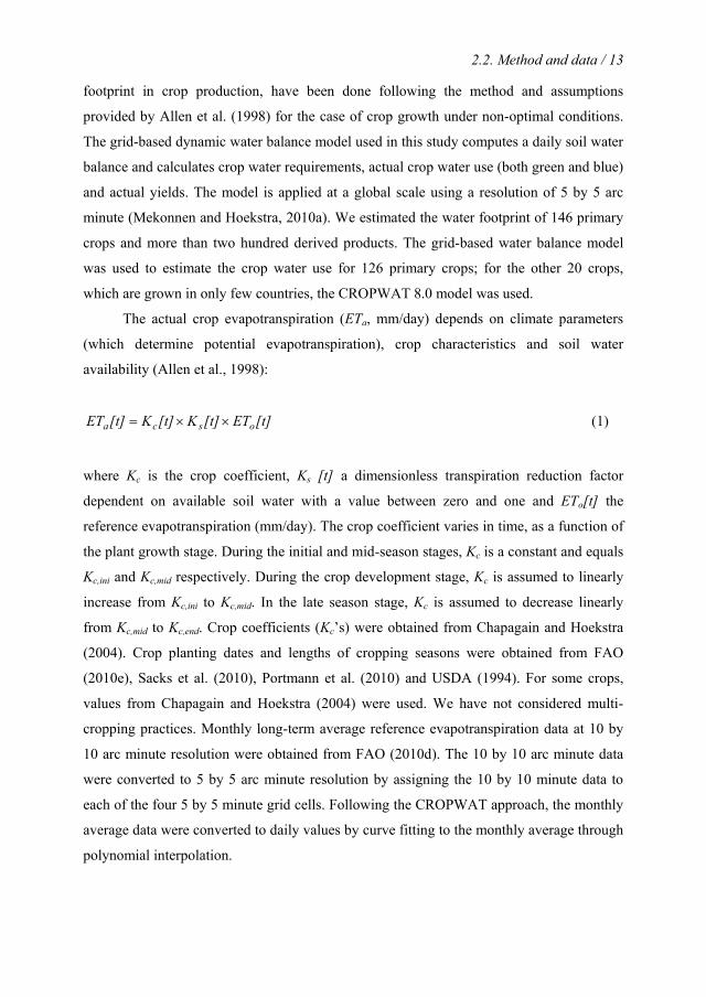
The actual crop evapotranspiration (ETa, mm/day) depends on climate parameters
(which determine potential evapotranspiration), crop characteristics and soil water
availability (Allen et al., 1998):
[t]ET[t]K[t]K[t]ET osca ××= (1)
where Kc is the crop coefficient, Ks [t] a dimensionless transpiration reduction factor
dependent on available soil water with a value between zero and one and ETo[t] the
reference evapotranspiration (mm/day). The crop coefficient varies in time, as a function of
the plant growth stage. During the initial and mid-season stages, Kc is a constant and equals
Kc,ini and Kc,mid respectively. During the crop development stage, Kc is assumed to linearly
increase from Kc,ini to Kc,mid. In the late season stage, Kc is assumed to decrease linearly
from Kc,mid to Kc,end. Crop coefficients (Kc’s) were obtained from Chapagain and Hoekstra
(2004). Crop planting dates and lengths of cropping seasons were obtained from FAO
(2010e), Sacks et al. (2010), Portmann et al. (2010) and USDA (1994). For some crops,
values from Chapagain and Hoekstra (2004) were used. We have not considered multi-
cropping practices. Monthly long-term average reference evapotranspiration data at 10 by
10 arc minute resolution were obtained from FAO (2010d). The 10 by 10 arc minute data
were converted to 5 by 5 arc minute resolution by assigning the 10 by 10 minute data to
each of the four 5 by 5 minute grid cells. Following the CROPWAT approach, the monthly
average data were converted to daily values by curve fitting to the monthly average through
polynomial interpolation.
14 / Chapter 2. The green, blue and grey water footprint of crops
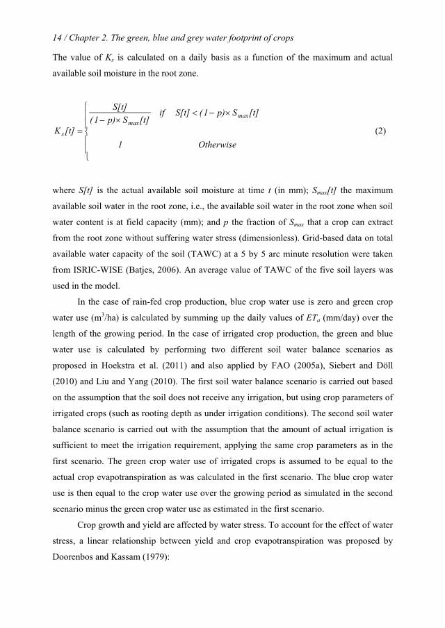
The value of Ks is calculated on a daily basis as a function of the maximum and actual
available soil moisture in the root zone.
×−<×−
=Otherwise1
[t]Sp)1(S[t]if[t]Sp)1(
S[t]
[t]K
maxmax
s (2)
where S[t] is the actual available soil moisture at time t (in mm); Smax[t] the maximum
available soil water in the root zone, i.e., the available soil water in the root zone when soil
water content is at field capacity (mm); and p the fraction of Smax that a crop can extract
from the root zone without suffering water stress (dimensionless). Grid-based data on total
available water capacity of the soil (TAWC) at a 5 by 5 arc minute resolution were taken
from ISRIC-WISE (Batjes, 2006). An average value of TAWC of the five soil layers was
used in the model.
In the case of rain-fed crop production, blue crop water use is zero and green crop
water use (m3/ha) is calculated by summing up the daily values of ETa (mm/day) over the
length of the growing period. In the case of irrigated crop production, the green and blue
water use is calculated by performing two different soil water balance scenarios as
proposed in Hoekstra et al. (2011) and also applied by FAO (2005a), Siebert and Döll
(2010) and Liu and Yang (2010). The first soil water balance scenario is carried out based
on the assumption that the soil does not receive any irrigation, but using crop parameters of
irrigated crops (such as rooting depth as under irrigation conditions). The second soil water
balance scenario is carried out with the assumption that the amount of actual irrigation is
sufficient to meet the irrigation requirement, applying the same crop parameters as in the
first scenario. The green crop water use of irrigated crops is assumed to be equal to the
actual crop evapotranspiration as was calculated in the first scenario. The blue crop water
use is then equal to the crop water use over the growing period as simulated in the second
scenario minus the green crop water use as estimated in the first scenario.
Crop growth and yield are affected by water stress. To account for the effect of water
stress, a linear relationship between yield and crop evapotranspiration was proposed by
Doorenbos and Kassam (1979):
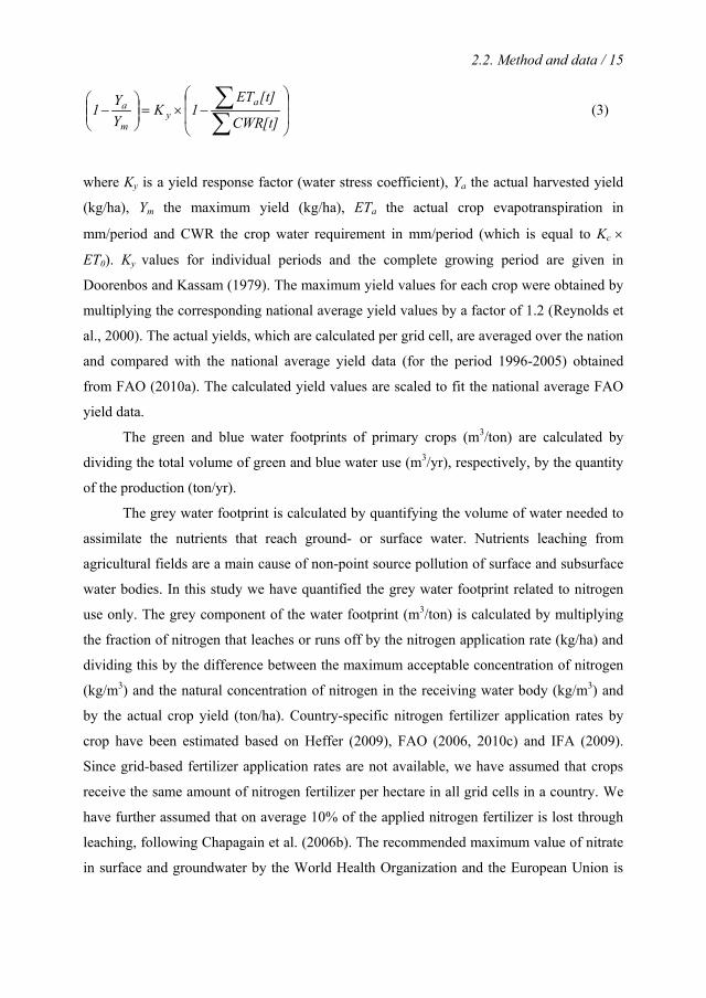
2.2. Method and data / 15
−×=
−
∑∑
[t]CWR
[t]ET1K
YY1 a
ym
a (3)
where Ky is a yield response factor (water stress coefficient), Ya the actual harvested yield
(kg/ha), Ym the maximum yield (kg/ha), ETa the actual crop evapotranspiration in
mm/period and CWR the crop water requirement in mm/period (which is equal to Kc ×
ET0). Ky values for individual periods and the complete growing period are given in
Doorenbos and Kassam (1979). The maximum yield values for each crop were obtained by
multiplying the corresponding national average yield values by a factor of 1.2 (Reynolds et
al., 2000). The actual yields, which are calculated per grid cell, are averaged over the nation
and compared with the national average yield data (for the period 1996-2005) obtained
from FAO (2010a). The calculated yield values are scaled to fit the national average FAO
yield data.
The green and blue water footprints of primary crops (m3/ton) are calculated by
dividing the total volume of green and blue water use (m3/yr), respectively, by the quantity
of the production (ton/yr).
The grey water footprint is calculated by quantifying the volume of water needed to
assimilate the nutrients that reach ground- or surface water. Nutrients leaching from
agricultural fields are a main cause of non-point source pollution of surface and subsurface
water bodies. In this study we have quantified the grey water footprint related to nitrogen
use only. The grey component of the water footprint (m3/ton) is calculated by multiplying
the fraction of nitrogen that leaches or runs off by the nitrogen application rate (kg/ha) and
dividing this by the difference between the maximum acceptable concentration of nitrogen
(kg/m3) and the natural concentration of nitrogen in the receiving water body (kg/m3) and
by the actual crop yield (ton/ha). Country-specific nitrogen fertilizer application rates by
crop have been estimated based on Heffer (2009), FAO (2006, 2010c) and IFA (2009).
Since grid-based fertilizer application rates are not available, we have assumed that crops
receive the same amount of nitrogen fertilizer per hectare in all grid cells in a country. We
have further assumed that on average 10% of the applied nitrogen fertilizer is lost through
leaching, following Chapagain et al. (2006b). The recommended maximum value of nitrate
in surface and groundwater by the World Health Organization and the European Union is

16 / Chapter 2. The green, blue and grey water footprint of crops
50 mg nitrate (NO3) per litre and the maximum value recommended by US-EPA is 10 mg
per litre measured as nitrate-nitrogen (NO3-N). In this study we have used the standard of
10 mg per litre of nitrate-nitrogen (NO3-N), following again Chapagain et al. (2006b).
Because of lack of data, the natural nitrogen concentrations were assumed to be zero.
The water footprints of crops as harvested have been used as a basis to calculate the
water footprints of derived crop products based on product and value fractions and water
footprints of processing steps following the method as in Hoekstra et al. (2011). For the
calculation of the water footprints of derived crop products we used product and value
fraction. Most of these fractions have been taken from FAO (2003) and Chapagain and
Hoekstra (2004). The product fraction of a product is defined as the quantity of output
product obtained per quantity of the primary input product. The value fraction of a product
is the ratio of the market value of the product to the aggregated market value of all the
products obtained from the input product (Hoekstra et al., 2011). Products and by-products
have both a product fraction and value fraction. On the other hand, residues (e.g. bran of
crops) have only a product fraction and we have assumed their value fraction to be close to
zero.
The water footprint per unit of energy for ethanol and biodiesel producing crops was
calculated following the method as applied in Gerbens-Leenes et al. (2009a). Data on the
dry mass of crops, the carbohydrate content of ethanol providing crops, the fat content of
biodiesel providing crops and the higher heating value of ethanol and biodiesel were taken
from Gerbens-Leenes et al. (2008a, 2008b) and summarized in Table 2.1.
Monthly values for precipitation, number of wet days and minimum and maximum
temperature for the period 1996-2002 with a spatial resolution of 30 by 30 arc minute were
obtained from CRU-TS-2.1 (Mitchell and Jones, 2005). The 30 by 30 arc minute data were
assigned to each of the thirty-six 5 by 5 arc minute grid cells contained in the 30 by 30 arc
minute grid cell. Daily precipitation values were generated from the monthly average
values using the CRU-dGen daily weather generator model (Schuol and Abbaspour, 2007).
Crop growing areas on a 5 by 5 arc minute grid cell resolution were obtained from
Monfreda et al. (2008). For countries missing grid data in Monfreda et al. (2008), the
MICRA2000 grid database as described in Portmann et al. (2010) was used to fill the gap.
The harvested crop areas as available in grid format were aggregated to a national level and
2.2. Method and data / 17
scaled to fit national average crop harvest areas for the period 1996-2005 obtained from
FAO (2010a).
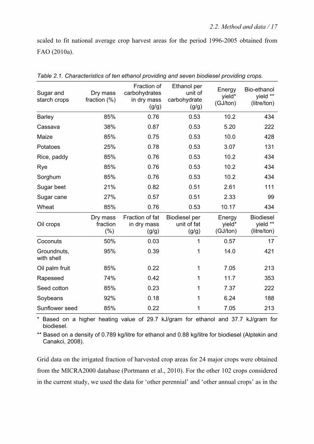
Table 2.1. Characteristics of ten ethanol providing and seven biodiesel providing crops.
Sugar and starch crops
Dry mass fraction (%)
Fraction of carbohydrates
in dry mass (g/g)
Ethanol per unit of
carbohydrate (g/g)
Energy yield*
(GJ/ton)
Bio-ethanol yield **
(litre/ton)
Barley 85% 0.76 0.53 10.2 434
Cassava 38% 0.87 0.53 5.20 222
Maize 85% 0.75 0.53 10.0 428
Potatoes 25% 0.78 0.53 3.07 131
Rice, paddy 85% 0.76 0.53 10.2 434
Rye 85% 0.76 0.53 10.2 434
Sorghum 85% 0.76 0.53 10.2 434
Sugar beet 21% 0.82 0.51 2.61 111
Sugar cane 27% 0.57 0.51 2.33 99
Wheat 85% 0.76 0.53 10.17 434
Oil crops Dry mass
fraction (%)
Fraction of fat in dry mass
(g/g)
Biodiesel per unit of fat
(g/g)
Energy yield*
(GJ/ton)
Biodiesel yield **
(litre/ton)
Coconuts 50% 0.03 1 0.57 17
Groundnuts, with shell
95% 0.39 1 14.0 421
Oil palm fruit 85% 0.22 1 7.05 213
Rapeseed 74% 0.42 1 11.7 353
Seed cotton 85% 0.23 1 7.37 222
Soybeans 92% 0.18 1 6.24 188
Sunflower seed 85% 0.22 1 7.05 213
* Based on a higher heating value of 29.7 kJ/gram for ethanol and 37.7 kJ/gram for biodiesel.
** Based on a density of 0.789 kg/litre for ethanol and 0.88 kg/litre for biodiesel (Alptekin and Canakci, 2008).
Grid data on the irrigated fraction of harvested crop areas for 24 major crops were obtained
from the MICRA2000 database (Portmann et al., 2010). For the other 102 crops considered
in the current study, we used the data for ‘other perennial’ and ‘other annual crops’ as in the
18 / Chapter 2. The green, blue and grey water footprint of crops
MICRA2000 database, depending on whether the crop is categorised under ‘perennial’ or
‘annual’ crops.
2.3 Result
2.3.1 The global picture
The global water footprint of crop production in the period 1996-2005 was 7404 Gm3/year
(78% green, 12% blue, and 10% grey). Wheat takes the largest share in this total volume; it
consumed 1087 Gm3/yr (70% green, 19% blue, 11% grey). The other crops with a large
total water footprint are rice (992 Gm3/yr) and maize (770 Gm3/yr). The contribution of the
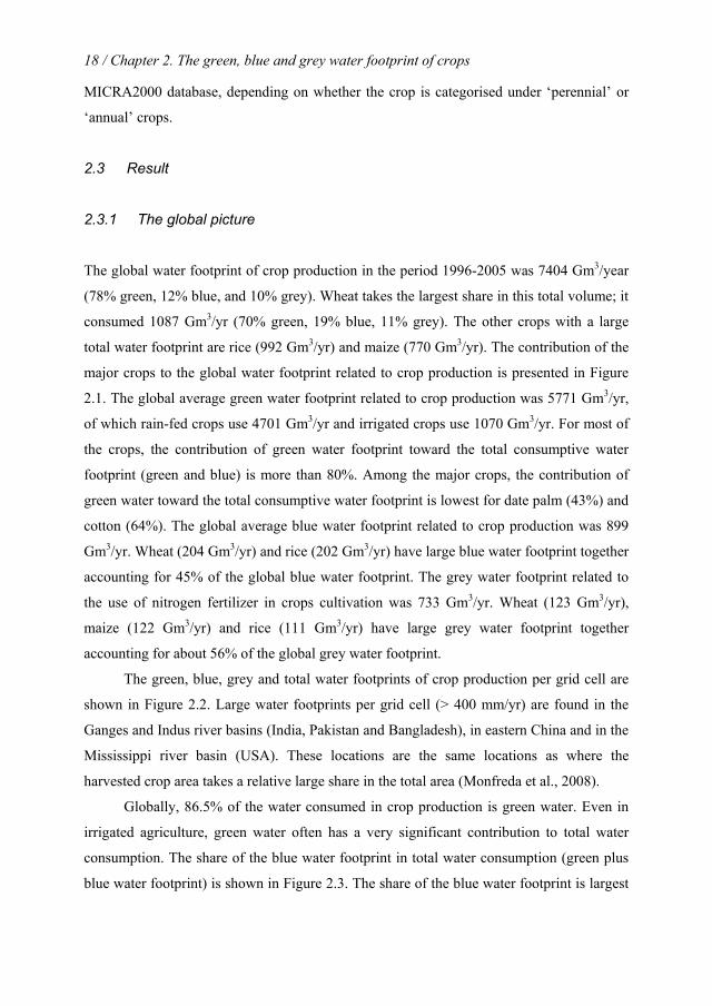
major crops to the global water footprint related to crop production is presented in Figure
2.1. The global average green water footprint related to crop production was 5771 Gm3/yr,
of which rain-fed crops use 4701 Gm3/yr and irrigated crops use 1070 Gm3/yr. For most of
the crops, the contribution of green water footprint toward the total consumptive water
footprint (green and blue) is more than 80%. Among the major crops, the contribution of
green water toward the total consumptive water footprint is lowest for date palm (43%) and
cotton (64%). The global average blue water footprint related to crop production was 899
Gm3/yr. Wheat (204 Gm3/yr) and rice (202 Gm3/yr) have large blue water footprint together
accounting for 45% of the global blue water footprint. The grey water footprint related to
the use of nitrogen fertilizer in crops cultivation was 733 Gm3/yr. Wheat (123 Gm3/yr),
maize (122 Gm3/yr) and rice (111 Gm3/yr) have large grey water footprint together
accounting for about 56% of the global grey water footprint.
The green, blue, grey and total water footprints of crop production per grid cell are
shown in Figure 2.2. Large water footprints per grid cell (> 400 mm/yr) are found in the
Ganges and Indus river basins (India, Pakistan and Bangladesh), in eastern China and in the
Mississippi river basin (USA). These locations are the same locations as where the
harvested crop area takes a relative large share in the total area (Monfreda et al., 2008).
Globally, 86.5% of the water consumed in crop production is green water. Even in
irrigated agriculture, green water often has a very significant contribution to total water
consumption. The share of the blue water footprint in total water consumption (green plus
blue water footprint) is shown in Figure 2.3. The share of the blue water footprint is largest
2.3. Results / 19
in arid and semi-arid regions. Regions with a large blue water proportion are located, for
example, in the western part of the USA, in a relatively narrow strip of land along the west
coast of South America (Peru-Chile), in southern Europe, North Africa, the Arabian
peninsula, Central Asia, Pakistan and northern India, northeast China and parts of Australia.
Wheat15%
Rice, paddy13%
Maize10%
Other28%
Coconuts2%
Oil palm2%
Sorghum2%
Barley3% Millet
2%
Coffee, green2%
Fodder crops9%
Soybeans5%
Sugar cane4%
Seed cotton3% Natural rubber
1%
Cassava1%
Groundnuts1%
Potatoes1%
Beans, dry1%
Rapeseed1%
Other crops21%
Figure 2.1. Contribution of different crops to the total water footprint of crop production. Period: 1996-2005.
2.3.2 The water footprint of primary crops and derived crop products per ton
The average water footprint per ton of primary crop differs significantly among crops and
across production regions. Crops with a high yield or large fraction of crop biomass that is
harvested generally have a smaller water footprint per ton than crops with a low yield or
small fraction of crop biomass harvested. When considered per ton of product, commodities
with relatively large water footprints are: coffee, tea, cocoa, tobacco, spices, nuts, rubber
and fibres (Table 2.2). For food crops, the global average water footprint per ton of crop
increases from sugar crops (roughly 200 m3/ton), vegetables (~300 m3/ton), roots and
tubers (~400 m3/ton), fruits (~1000 m3/ton), cereals (~1600 m3/ton), oil crops (~2400
m3/ton), pulses (~4000 m3/ton), spices (~7000 m3/ton) to nuts (~9000 m3/ton). The water
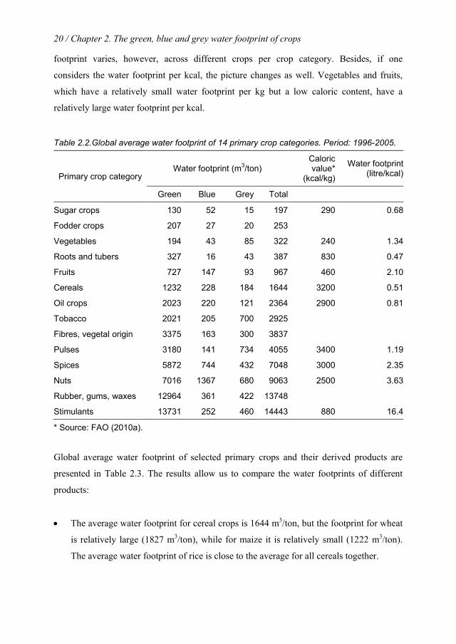
20 / Chapter 2. The green, blue and grey water footprint of crops
footprint varies, however, across different crops per crop category. Besides, if one
considers the water footprint per kcal, the picture changes as well. Vegetables and fruits,
which have a relatively small water footprint per kg but a low caloric content, have a
relatively large water footprint per kcal.
Table 2.2.Global average water footprint of 14 primary crop categories. Period: 1996-2005.
Primary crop category Water footprint (m3/ton)
Caloric value*
(kcal/kg)
Water footprint (litre/kcal)
Green Blue Grey Total
Sugar crops 130 52 15 197 290 0.68
Fodder crops 207 27 20 253
Vegetables 194 43 85 322 240 1.34
Roots and tubers 327 16 43 387 830 0.47
Fruits 727 147 93 967 460 2.10
Cereals 1232 228 184 1644 3200 0.51
Oil crops 2023 220 121 2364 2900 0.81
Tobacco 2021 205 700 2925
Fibres, vegetal origin 3375 163 300 3837
Pulses 3180 141 734 4055 3400 1.19
Spices 5872 744 432 7048 3000 2.35
Nuts 7016 1367 680 9063 2500 3.63
Rubber, gums, waxes 12964 361 422 13748
Stimulants 13731 252 460 14443 880 16.4
* Source: FAO (2010a).
Global average water footprint of selected primary crops and their derived products are
presented in Table 2.3. The results allow us to compare the water footprints of different
products:
• The average water footprint for cereal crops is 1644 m3/ton, but the footprint for wheat
is relatively large (1827 m3/ton), while for maize it is relatively small (1222 m3/ton).
The average water footprint of rice is close to the average for all cereals together.
2.3. Results / 21
• Sugar obtained from sugar beet has a smaller water footprint than sugar from sugar
cane. Besides, the blue component in the total water footprint of beet sugar (20%) is
smaller than for cane sugar (27%).
• For vegetable oils we find a large variation in water footprints: maize oil 2600 m3/ton;
cotton-seed oil 3800 m3/ton; soybean oil 4200 m3/ton; rapeseed oil 4300 m3/ton; palm
oil 5000 m3/ton; sunflower oil 6800 m3/ton; groundnut oil 7500 m3/ton; linseed oil
9400 m3/ton; olive oil 14500 m3/ton; castor oil 24700 m3/ton.
• For fruits we find a similar variation in water footprints: water melon 235 m3/ton;
pineapple 255 m3/ton; papaya 460 m3/ton; orange 560 m3/ton; banana 790 m3/ton;
apple 820 m3/ton; peach 910 m3/ton; pear 920 m3/ton; apricot 1300 m3/ton; plums 2200
m3/ton; dates 2300 m3/ton; grapes 2400 m3/ton; figs 3350 m3/ton.
• For alcoholic beverages we find: a water footprint of 300 m3/ton for beer and 870
m3/ton for wine.
• The water footprints of juices vary from tomato juice (270 m3/ton), grapefruit juice
(675 m3/ton), orange juice (1000 m3/ton) and apple juice (1100 m3/ton) to pineapple
juice (1300 m3/ton).
• The water footprint of coffee (130 litre/cup, based on use of 7 gram of roasted coffee
per cup) is much larger than the water footprint of tea (27 litre/cup, based on use of 3
gram of black tea per cup).
• The water footprint of cotton fibres is substantially larger than the water footprints of
sisal and flax fibres, which are again larger than the water footprints of jute and hemp
fibres.
One should be careful in drawing conclusions from the above product comparisons.
Although the global average water footprint of one product may be larger than the global
average water footprint of another product, the comparison may turn out quite differently
for specific regions.
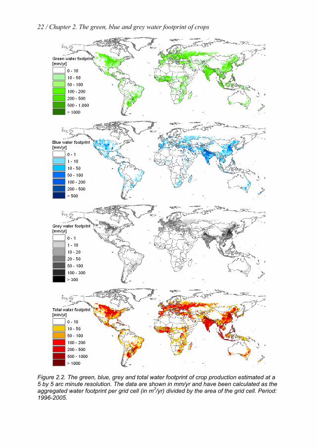
22 / Chapter 2. The green, blue and grey water footprint of crops
Figure 2.2. The green, blue, grey and total water footprint of crop production estimated at a 5 by 5 arc minute resolution. The data are shown in mm/yr and have been calculated as the aggregated water footprint per grid cell (in m3/yr) divided by the area of the grid cell. Period: 1996-2005.
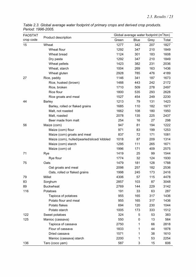
2.3. Results / 23
Table 2.3. Global average water footprint of primary crops and derived crop products. Period: 1996-2005. FAOSTAT crop code
Product description Global average water footprint (m3/ton) Green Blue Grey Total
15 Wheat 1277 342 207 1827 Wheat flour 1292 347 210 1849 Wheat bread 1124 301 183 1608 Dry pasta 1292 347 210 1849 Wheat pellets 1423 382 231 2036 Wheat, starch 1004 269 163 1436 Wheat gluten 2928 785 476 4189 27 Rice, paddy 1146 341 187 1673 Rice, husked (brown) 1488 443 242 2172 Rice, broken 1710 509 278 2497 Rice flour 1800 535 293 2628 Rice groats and meal 1527 454 249 2230 44 Barley 1213 79 131 1423 Barley, rolled or flaked grains 1685 110 182 1977 Malt, not roasted 1662 108 180 1950 Malt, roasted 2078 135 225 2437 Beer made from malt 254 16 27 298 56 Maize (corn) 947 81 194 1222 Maize (corn) flour 971 83 199 1253 Maize (corn) groats and meal 837 72 171 1081 Maize (corn), hulled/pearled/sliced/ kibbled 1018 87 209 1314 Maize (corn) starch 1295 111 265 1671 Maize (corn) oil 1996 171 409 2575 71 Rye 1419 25 99 1544 Rye flour 1774 32 124 1930 75 Oats 1479 181 128 1788 Oat groats and meal 2098 257 182 2536 Oats, rolled or flaked grains 1998 245 173 2416 79 Millet 4306 57 115 4478 83 Sorghum 2857 103 87 3048 89 Buckwheat 2769 144 229 3142 116 Potatoes 191 33 63 287 Tapioca of potatoes 955 165 317 1436 Potato flour and meal 955 165 317 1436 Potato flakes 694 120 230 1044 Potato starch 1005 173 333 1512 122 Sweet potatoes 324 5 53 383 125 Manioc (cassava) 550 0 13 564 Tapioca of cassava 2750 1 66 2818 Flour of cassava 1833 1 44 1878 Dried cassava 1571 1 38 1610 Manioc (cassava) starch 2200 1 53 2254 136 Taro (coco yam) 587 3 15 606
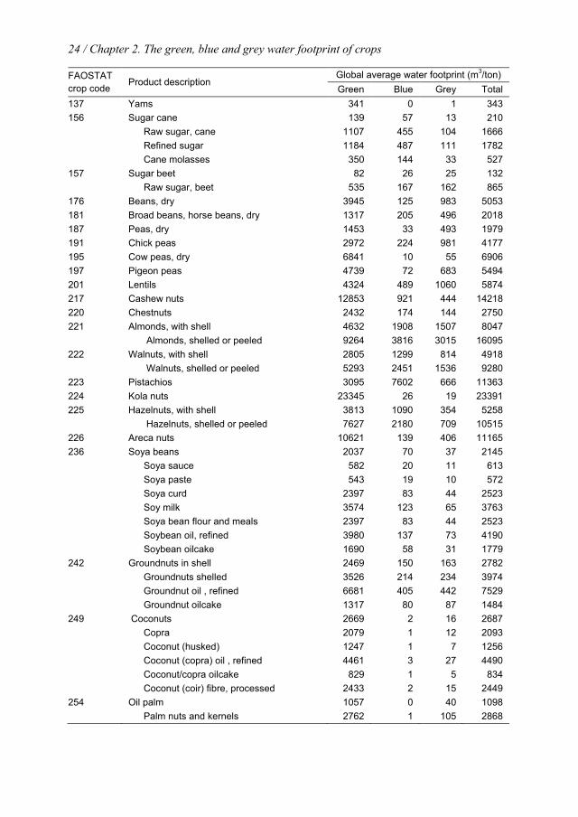
24 / Chapter 2. The green, blue and grey water footprint of crops
FAOSTAT crop code
Product description Global average water footprint (m3/ton) Green Blue Grey Total
137 Yams 341 0 1 343 156 Sugar cane 139 57 13 210 Raw sugar, cane 1107 455 104 1666 Refined sugar 1184 487 111 1782 Cane molasses 350 144 33 527 157 Sugar beet 82 26 25 132 Raw sugar, beet 535 167 162 865 176 Beans, dry 3945 125 983 5053 181 Broad beans, horse beans, dry 1317 205 496 2018 187 Peas, dry 1453 33 493 1979 191 Chick peas 2972 224 981 4177 195 Cow peas, dry 6841 10 55 6906 197 Pigeon peas 4739 72 683 5494 201 Lentils 4324 489 1060 5874 217 Cashew nuts 12853 921 444 14218 220 Chestnuts 2432 174 144 2750 221 Almonds, with shell 4632 1908 1507 8047 Almonds, shelled or peeled 9264 3816 3015 16095 222 Walnuts, with shell 2805 1299 814 4918 Walnuts, shelled or peeled 5293 2451 1536 9280 223 Pistachios 3095 7602 666 11363 224 Kola nuts 23345 26 19 23391 225 Hazelnuts, with shell 3813 1090 354 5258 Hazelnuts, shelled or peeled 7627 2180 709 10515 226 Areca nuts 10621 139 406 11165 236 Soya beans 2037 70 37 2145 Soya sauce 582 20 11 613 Soya paste 543 19 10 572 Soya curd 2397 83 44 2523 Soy milk 3574 123 65 3763 Soya bean flour and meals 2397 83 44 2523 Soybean oil, refined 3980 137 73 4190 Soybean oilcake 1690 58 31 1779 242 Groundnuts in shell 2469 150 163 2782 Groundnuts shelled 3526 214 234 3974 Groundnut oil , refined 6681 405 442 7529 Groundnut oilcake 1317 80 87 1484 249 Coconuts 2669 2 16 2687 Copra 2079 1 12 2093 Coconut (husked) 1247 1 7 1256 Coconut (copra) oil , refined 4461 3 27 4490 Coconut/copra oilcake 829 1 5 834 Coconut (coir) fibre, processed 2433 2 15 2449 254 Oil palm 1057 0 40 1098 Palm nuts and kernels 2762 1 105 2868

2.3. Results / 25
FAOSTAT crop code
Product description Global average water footprint (m3/ton) Green Blue Grey Total
Palm oil, refined 4787 1 182 4971 Palm kernel/babassu oil, refined 5202 1 198 5401 Palm nut/kernel oilcake 802 0 31 833 260 Olives 2470 499 45 3015 Olive oil, virgin 11826 2388 217 14431 Olive oil, refined 12067 2437 221 14726 265 Castor oil seeds 8423 1175 298 9896 Castor oil 21058 2938 744 24740 267 Sunflower seeds 3017 148 201 3366 Sunflower seed oil, refined 6088 299 405 6792 Sunflower seed oilcake 1215 60 81 1356 270 Rapeseed 1703 231 336 2271 Rape oil, refined 3226 438 636 4301 Rape seed oilcake 837 114 165 1115 280 Safflower seeds 6000 938 283 7221 289 Sesame seed 8460 509 403 9371 Sesame oil 19674 1183 936 21793 292 Mustard seeds 2463 1 345 2809 296 Poppy seeds 1723 0 464 2188 299 Melon seed 5087 56 41 5184 328 Seed cotton 2282 1306 440 4029 Cotton seeds 755 432 146 1332 Cotton lint 5163 2955 996 9113 Cotton linters 1474 844 284 2602 Cotton-seed oil, refined 2242 1283 432 3957 Cotton seed oilcake 487 279 94 860 Cotton, not carded or combed 5163 2955 996 9113 Cotton yarn & thread waste 950 544 183 1677 Garneted stock of cotton 1426 816 275 2517 Cotton, carded or combed 5359 3067 1034 9460 Cotton fabric, finished textile 5384 3253 1344 9982 333 Linseed 4730 268 170 5168 Linseed oil, refined 8618 488 310 9415 Linseed oilcake 2816 160 101 3077 336 Hempseed 3257 12 417 3685 358 Cabbages and other brassicas 181 26 73 280 366 Artichokes 478 242 98 818 367 Asparagus 1524 119 507 2150 372 Lettuce 133 28 77 237 373 Spinach 118 14 160 292 388 Tomatoes 108 63 43 214 Tomato juice unfermented/not spirited 135 79 53 267 Tomato juice, concentrated 539 316 213 1069 Tomato paste 431 253 171 855 Tomato ketchup 270 158 107 534

26 / Chapter 2. The green, blue and grey water footprint of crops
FAOSTAT crop code
Product description Global average water footprint (m3/ton) Green Blue Grey Total
Tomato puree 360 211 142 713 Peeled tomatoes 135 79 53 267 Tomato, dried 2157 1265 853 4276 393 Cauliflowers and broccoli 189 21 75 285 Brussels sprouts 189 21 75 285 394 Pumpkins, squash and gourds 228 24 84 336 397 Cucumbers and gherkins 206 42 105 353 399 Eggplants (aubergines) 234 33 95 362 401 Chillies and peppers, green 240 42 97 379 402 Onions (incl. shallots), green 176 44 51 272 403 Onions, dry 192 88 65 345 406 Garlic 337 81 170 589 Garlic powder 1297 313 655 2265 414 Beans, green 320 54 188 561 417 Peas, green 382 63 150 595 423 String beans 301 104 143 547 426 Carrots and turnips 106 28 61 195 430 Okra 474 36 65 576 446 Maize, green 455 157 88 700 461 Carobs 4557 334 703 5594 486 Bananas 660 97 33 790 489 Plantains 1570 27 6 1602 490 Oranges 401 110 49 560 Orange juice 729 199 90 1018 495 Tangerines, mandarins, clement 479 118 152 748 497 Lemons and limes 432 152 58 642 507 Grapefruit 367 85 54 506 515 Apples, fresh 561 133 127 822 Apples, dried 4678 1111 1058 6847 Apple juice unfermented/ not spirited 780 185 176 1141 521 Pears 645 94 183 922 526 Apricots 694 502 92 1287 530 Sour cherries 1098 213 99 1411 531 Cherries 961 531 112 1604 534 Peaches and nectarines 583 188 139 910 536 Plums and sloes 1570 188 422 2180 544 Strawberries 201 109 37 347 547 Raspberries 293 53 67 413 549 Gooseberries 487 8 31 526 550 Currants 457 19 23 499 552 Blueberries 341 334 170 845 554 Cranberries 91 108 77 276 560 Grapes 425 97 87 608 Grapes, dried 1700 386 347 2433 Grapefruit juice 490 114 71 675
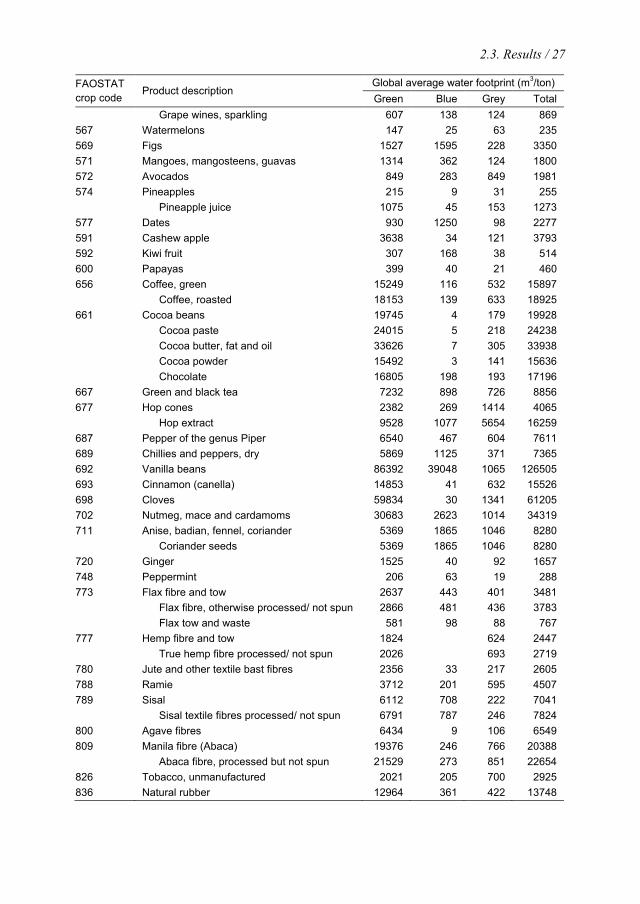
2.3. Results / 27
FAOSTAT crop code
Product description Global average water footprint (m3/ton) Green Blue Grey Total
Grape wines, sparkling 607 138 124 869 567 Watermelons 147 25 63 235 569 Figs 1527 1595 228 3350 571 Mangoes, mangosteens, guavas 1314 362 124 1800 572 Avocados 849 283 849 1981 574 Pineapples 215 9 31 255 Pineapple juice 1075 45 153 1273 577 Dates 930 1250 98 2277 591 Cashew apple 3638 34 121 3793 592 Kiwi fruit 307 168 38 514 600 Papayas 399 40 21 460 656 Coffee, green 15249 116 532 15897 Coffee, roasted 18153 139 633 18925 661 Cocoa beans 19745 4 179 19928 Cocoa paste 24015 5 218 24238 Cocoa butter, fat and oil 33626 7 305 33938 Cocoa powder 15492 3 141 15636 Chocolate 16805 198 193 17196 667 Green and black tea 7232 898 726 8856 677 Hop cones 2382 269 1414 4065 Hop extract 9528 1077 5654 16259 687 Pepper of the genus Piper 6540 467 604 7611 689 Chillies and peppers, dry 5869 1125 371 7365 692 Vanilla beans 86392 39048 1065 126505 693 Cinnamon (canella) 14853 41 632 15526 698 Cloves 59834 30 1341 61205 702 Nutmeg, mace and cardamoms 30683 2623 1014 34319 711 Anise, badian, fennel, coriander 5369 1865 1046 8280 Coriander seeds 5369 1865 1046 8280 720 Ginger 1525 40 92 1657 748 Peppermint 206 63 19 288 773 Flax fibre and tow 2637 443 401 3481 Flax fibre, otherwise processed/ not spun 2866 481 436 3783 Flax tow and waste 581 98 88 767 777 Hemp fibre and tow 1824 624 2447 True hemp fibre processed/ not spun 2026 693 2719 780 Jute and other textile bast fibres 2356 33 217 2605 788 Ramie 3712 201 595 4507 789 Sisal 6112 708 222 7041 Sisal textile fibres processed/ not spun 6791 787 246 7824 800 Agave fibres 6434 9 106 6549 809 Manila fibre (Abaca) 19376 246 766 20388 Abaca fibre, processed but not spun 21529 273 851 22654 826 Tobacco, unmanufactured 2021 205 700 2925 836 Natural rubber 12964 361 422 13748
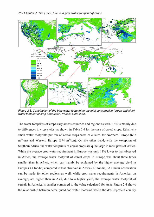
28 / Chapter 2. The green, blue and grey water footprint of crops
Figure 2.3. Contribution of the blue water footprint to the total consumptive (green and blue) water footprint of crop production. Period: 1996-2005.
The water footprints of crops vary across countries and regions as well. This is mainly due
to differences in crop yields, as shown in Table 2.4 for the case of cereal crops. Relatively
small water footprints per ton of cereal crops were calculated for Northern Europe (637
m3/ton) and Western Europe (654 m3/ton). On the other hand, with the exception of
Southern Africa, the water footprints of cereal crops are quite large in most parts of Africa.
While the average crop water requirement in Europe was only 11% lower to that observed
in Africa, the average water footprint of cereal crops in Europe was about three times
smaller than in Africa, which can mainly be explained by the higher average yield in
Europe (3.4 ton/ha) compared to that observed in Africa (1.3 ton/ha). A similar observation
can be made for other regions as well: while crop water requirements in America, on
average, are higher than in Asia, due to a higher yield, the average water footprint of
cereals in America is smaller compared to the value calculated for Asia. Figure 2.4 shows
the relationship between cereal yield and water footprint, where the dots represent country
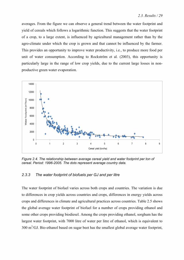
2.3. Results / 29
averages. From the figure we can observe a general trend between the water footprint and
yield of cereals which follows a logarithmic function. This suggests that the water footprint
of a crop, to a large extent, is influenced by agricultural management rather than by the
agro-climate under which the crop is grown and that cannot be influenced by the farmer.
This provides an opportunity to improve water productivity, i.e., to produce more food per
unit of water consumption. According to Rockström et al. (2003), this opportunity is
particularly large in the range of low crop yields, due to the current large losses in non-
productive green water evaporation.
0
2000
4000
6000
8000
10000
12000
14000
0 1 2 3 4 5 6 7 8 9
Wat
er f
oo
tprin
t (m
3/t
on)
Cereal yield (ton/ha)
Figure 2.4. The relationship between average cereal yield and water footprint per ton of cereal. Period: 1996-2005. The dots represent average country data.
2.3.3 The water footprint of biofuels per GJ and per litre
The water footprint of biofuel varies across both crops and countries. The variation is due
to differences in crop yields across countries and crops, differences in energy yields across
crops and differences in climate and agricultural practices across countries. Table 2.5 shows
the global average water footprint of biofuel for a number of crops providing ethanol and
some other crops providing biodiesel. Among the crops providing ethanol, sorghum has the
largest water footprint, with 7000 litre of water per litre of ethanol, which is equivalent to
300 m3/GJ. Bio-ethanol based on sugar beet has the smallest global average water footprint,
30 / Chapter 2. The green, blue and grey water footprint of crops
with 1200 litre of water per litre of ethanol, equivalent to 50 m3/GJ. In general, biodiesel
has a larger water footprint per unit of energy obtained than bio-ethanol, a finding that is
consistent with Gerbens-Leenes et al. (2009a). Among the crops studied here, biodiesel
from coconuts has the largest water footprint: 4750 m3/GJ. Biodiesels from oil palm,
rapeseed and groundnuts are more efficient, with water footprints in the range 150-200
m3/GJ. The largest blue water footprint is observed for biodiesel from cotton: 177 m3/GJ
(32% of the total water footprint).
2.3.4 The total water footprint of crop production at national and sub-national
level
At the country level, the largest total water footprints were estimated for India, China, the
USA, Brazil, Russia and Indonesia. These six countries together account for about half of
the global total water footprint related to crop production. The largest green water
footprints are also found in these six countries: India, China, the USA, Russia, Brazil and
Indonesia. Data per country are shown in Table 2.6 for the largest producers. At sub-
national level (state or province level), the largest green water footprints can be found in
Uttar Pradesh (88 Gm3/yr), Maharashtra (86 Gm3/yr), Karnataka (65 Gm3/yr), Andhra
Pradesh (61 Gm3/yr), and Madhya Pradesh (60 Gm3/yr), all in India. The largest blue water
footprints were calculated for India, China, the USA and Pakistan. These four countries
together account for 58% of the total blue water footprint related to crop production. At
sub-national level, the largest blue water footprints were found in: Uttar Pradesh (59
Gm3/yr) and Madhya Pradesh (24 Gm3/yr) in India; Punjab (50 Gm3/yr) in Pakistan; and
California (20 Gm3/yr) in the USA. Large grey water footprints were estimated for China,
the USA and India.
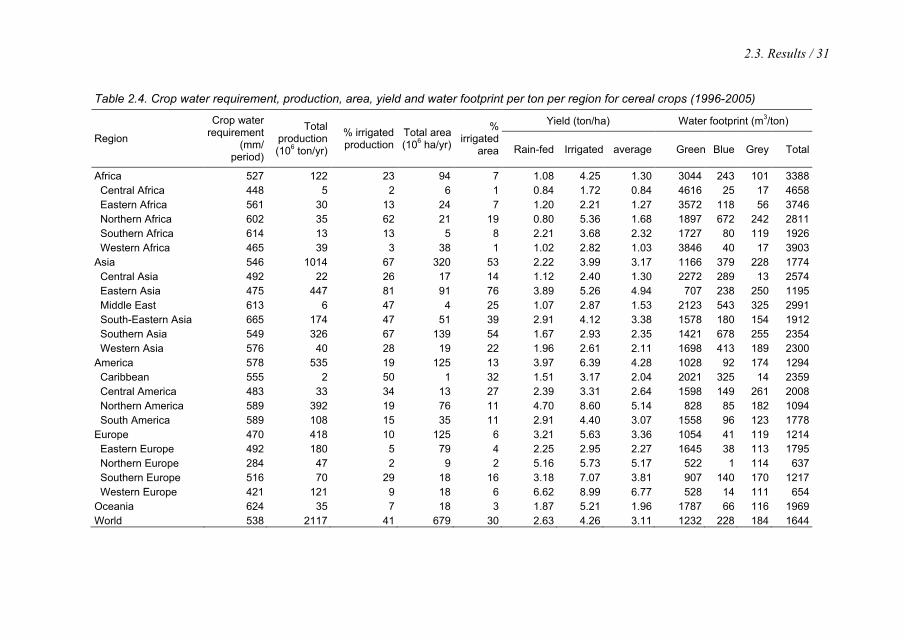
2.3. Results / 31
Table 2.4. Crop water requirement, production, area, yield and water footprint per ton per region for cereal crops (1996-2005)
Region
Crop water requirement
(mm/ period)
Total production (106 ton/yr)
% irrigated production
Total area (106 ha/yr)
% irrigated
area
Yield (ton/ha) Water footprint (m3/ton)
Rain-fed Irrigated average Green Blue Grey Total
Africa 527 122 23 94 7 1.08 4.25 1.30 3044 243 101 3388 Central Africa 448 5 2 6 1 0.84 1.72 0.84 4616 25 17 4658 Eastern Africa 561 30 13 24 7 1.20 2.21 1.27 3572 118 56 3746 Northern Africa 602 35 62 21 19 0.80 5.36 1.68 1897 672 242 2811 Southern Africa 614 13 13 5 8 2.21 3.68 2.32 1727 80 119 1926 Western Africa 465 39 3 38 1 1.02 2.82 1.03 3846 40 17 3903
Asia 546 1014 67 320 53 2.22 3.99 3.17 1166 379 228 1774 Central Asia 492 22 26 17 14 1.12 2.40 1.30 2272 289 13 2574 Eastern Asia 475 447 81 91 76 3.89 5.26 4.94 707 238 250 1195 Middle East 613 6 47 4 25 1.07 2.87 1.53 2123 543 325 2991 South-Eastern Asia 665 174 47 51 39 2.91 4.12 3.38 1578 180 154 1912 Southern Asia 549 326 67 139 54 1.67 2.93 2.35 1421 678 255 2354 Western Asia 576 40 28 19 22 1.96 2.61 2.11 1698 413 189 2300
America 578 535 19 125 13 3.97 6.39 4.28 1028 92 174 1294 Caribbean 555 2 50 1 32 1.51 3.17 2.04 2021 325 14 2359 Central America 483 33 34 13 27 2.39 3.31 2.64 1598 149 261 2008 Northern America 589 392 19 76 11 4.70 8.60 5.14 828 85 182 1094 South America 589 108 15 35 11 2.91 4.40 3.07 1558 96 123 1778
Europe 470 418 10 125 6 3.21 5.63 3.36 1054 41 119 1214 Eastern Europe 492 180 5 79 4 2.25 2.95 2.27 1645 38 113 1795 Northern Europe 284 47 2 9 2 5.16 5.73 5.17 522 1 114 637 Southern Europe 516 70 29 18 16 3.18 7.07 3.81 907 140 170 1217 Western Europe 421 121 9 18 6 6.62 8.99 6.77 528 14 111 654
Oceania 624 35 7 18 3 1.87 5.21 1.96 1787 66 116 1969 World 538 2117 41 679 30 2.63 4.26 3.11 1232 228 184 1644
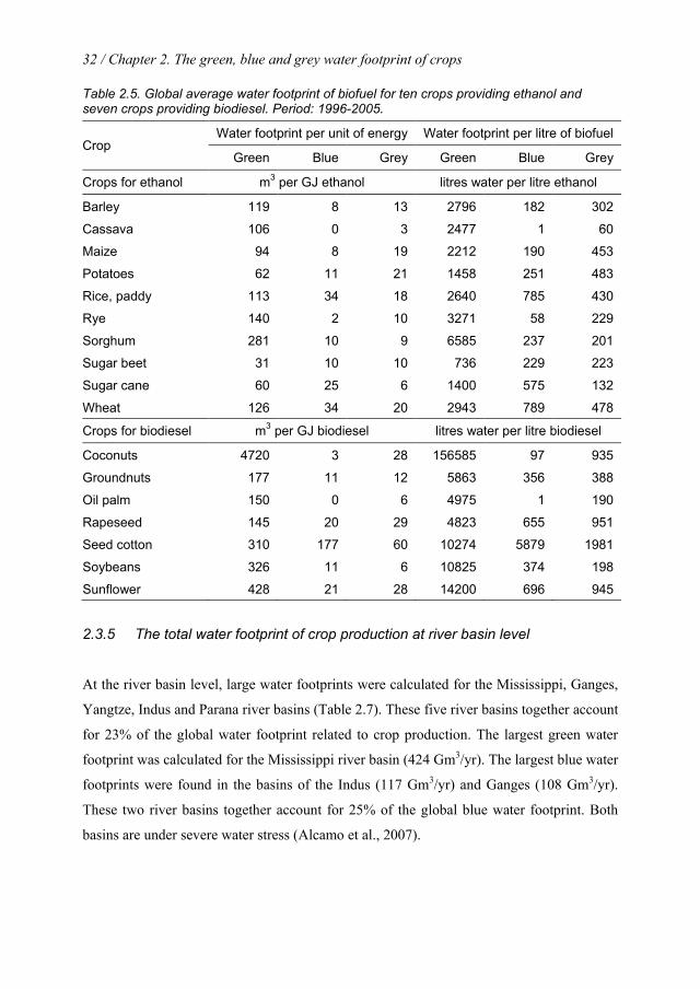
32 / Chapter 2. The green, blue and grey water footprint of crops
Table 2.5. Global average water footprint of biofuel for ten crops providing ethanol and seven crops providing biodiesel. Period: 1996-2005.
Crop Water footprint per unit of energy Water footprint per litre of biofuel
Green Blue Grey Green Blue Grey
Crops for ethanol m3 per GJ ethanol litres water per litre ethanol
Barley 119 8 13 2796 182 302
Cassava 106 0 3 2477 1 60
Maize 94 8 19 2212 190 453
Potatoes 62 11 21 1458 251 483
Rice, paddy 113 34 18 2640 785 430
Rye 140 2 10 3271 58 229
Sorghum 281 10 9 6585 237 201
Sugar beet 31 10 10 736 229 223
Sugar cane 60 25 6 1400 575 132
Wheat 126 34 20 2943 789 478
Crops for biodiesel m3 per GJ biodiesel litres water per litre biodiesel
Coconuts 4720 3 28 156585 97 935
Groundnuts 177 11 12 5863 356 388
Oil palm 150 0 6 4975 1 190
Rapeseed 145 20 29 4823 655 951
Seed cotton 310 177 60 10274 5879 1981
Soybeans 326 11 6 10825 374 198
Sunflower 428 21 28 14200 696 945
2.3.5 The total water footprint of crop production at river basin level
At the river basin level, large water footprints were calculated for the Mississippi, Ganges,
Yangtze, Indus and Parana river basins (Table 2.7). These five river basins together account
for 23% of the global water footprint related to crop production. The largest green water
footprint was calculated for the Mississippi river basin (424 Gm3/yr). The largest blue water
footprints were found in the basins of the Indus (117 Gm3/yr) and Ganges (108 Gm3/yr).
These two river basins together account for 25% of the global blue water footprint. Both
basins are under severe water stress (Alcamo et al., 2007).
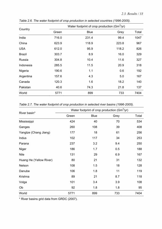
2.3. Results / 33
Table 2.6. The water footprint of crop production in selected countries (1996-2005).
Country Water footprint of crop production (Gm3/yr)
Green Blue Grey Total
India 716.0 231.4 99.4 1047
China 623.9 118.9 223.8 967
USA 612.0 95.9 118.2 826
Brazil 303.7 8.9 16.0 329
Russia 304.8 10.4 11.6 327
Indonesia 285.5 11.5 20.9 318
Nigeria 190.6 1.1 0.6 192
Argentina 157.6 4.3 5.0 167
Canada 120.3 1.6 18.2 140
Pakistan 40.6 74.3 21.8 137
World 5771 899 733 7404
Table 2.7. The water footprint of crop production in selected river basins (1996-2005).
River basin* Water footprint of crop production (Gm3/yr)
Green Blue Grey Total
Mississippi 424 40 70 534
Ganges 260 108 39 408
Yangtze (Chang Jiang) 177 18 61 256
Indus 102 117 34 253
Parana 237 3.2 9.4 250
Niger 186 1.7 0.5 188
Nile 131 29 6.9 167
Huang He (Yellow River) 80 21 31 132
Nelson 108 1.5 18 128
Danube 106 1.8 11 119
Krishna 89 21 8.7 118
Volga 101 3.4 3.9 108
Ob 92 1.8 1.8 95
World 5771 899 733 7404
* River basins grid data from GRDC (2007).
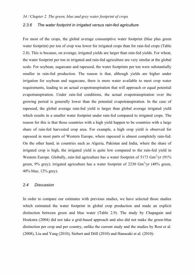
34 / Chapter 2. The green, blue and grey water footprint of crops
2.3.6 The water footprint in irrigated versus rain-fed agriculture
For most of the crops, the global average consumptive water footprint (blue plus green
water footprint) per ton of crop was lower for irrigated crops than for rain-fed crops (Table
2.8). This is because, on average, irrigated yields are larger than rain-fed yields. For wheat,
the water footprint per ton in irrigated and rain-fed agriculture are very similar at the global
scale. For soybean, sugarcane and rapeseed, the water footprints per ton were substantially
smaller in rain-fed production. The reason is that, although yields are higher under
irrigation for soybean and sugarcane, there is more water available to meet crop water
requirements, leading to an actual evapotranspiration that will approach or equal potential
evapotranspiration. Under rain-fed conditions, the actual evapotranspiration over the
growing period is generally lower than the potential evapotranspiration. In the case of
rapeseed, the global average rain-fed yield is larger than global average irrigated yield
which results in a smaller water footprint under rain-fed compared to irrigated crops. The
reason for this is that those countries with a high yield happen to be countries with a large
share of rain-fed harvested crop area. For example, a high crop yield is observed for
rapeseed in most parts of Western Europe, where rapeseed is almost completely rain-fed.
On the other hand, in countries such as Algeria, Pakistan and India, where the share of
irrigated crop is high, the irrigated yield is quite low compared to the rain-fed yield in
Western Europe. Globally, rain-fed agriculture has a water footprint of 5173 Gm3/yr (91%
green, 9% grey); irrigated agriculture has a water footprint of 2230 Gm3/yr (48% green,
40% blue, 12% grey).
2.4 Discussion
In order to compare our estimates with previous studies, we have selected those studies
which estimated the water footprint in global crop production and made an explicit
distinction between green and blue water (Table 2.9). The study by Chapagain and
Hoekstra (2004) did not take a grid-based approach and also did not make the green-blue
distinction per crop and per country, unlike the current study and the studies by Rost et al.
(2008), Liu and Yang (2010), Siebert and Döll (2010) and Hanasaki et al. (2010).

2.4. Discussion / 35
Table 2.8. The water footprint of rain-fed and irrigated agriculture for selected crops (1996-2005).
Crop
Farming system
Yield (ton/ha)
Total water footprint related to crop production (Gm3/yr)
Water footprint per ton of crop (m3/ton)
Green Blue Grey Total Green Blue Grey Rain-fed 2.48 610 0 65 676 1629 0 175 Wheat Irrigated 3.31 150 204 58 411 679 926 263 Global 2.74 760 204 123 1087 1278 342 208 Rain-fed 4.07 493 0 85 579 1082 0 187 Maize Irrigated 6.01 104 51 37 192 595 294 212 Global 4.47 597 51 122 770 947 81 194 Rain-fed 2.69 301 0 30 331 1912 0 190 Rice Irrigated 4.67 378 202 81 661 869 464 185 Global 3.90 679 202 111 992 1146 341 187 Rain-fed 8.93 24 0 6 30 717 0 167 Apples Irrigated 15.91 8 8 2 18 343 321 71 Global 10.92 33 8 7 48 561 133 127 Rain-fed 2.22 328 0 5 333 2079 0 33 Soybean Irrigated 2.48 24 12 1 37 1590 926 85 Global 2.24 351 12 6 370 2037 70 37 Rain-fed 58.70 95 0 7 102 164 0 13 Sugarcane Irrigated 71.17 85 74 10 169 120 104 14 Global 64.96 180 74 17 271 139 57 13 Rain-fed 0.68 106 0 4 110 15251 0 523 Coffee Irrigated 0.98 1 1 0 2 8668 4974 329 Global 0.69 108 1 4 112 15249 116 532 Rain-fed 1.63 62 0 12 74 1783 0 356 Rapeseed Irrigated 1.23 4 9 1 14 1062 2150 181 Global 1.57 66 9 13 88 1703 231 336 Rain-fed 1.35 90 0 13 103 3790 0 532 Cotton Irrigated 2.16 41 75 13 129 1221 2227 376 Global 1.73 132 75 25 233 2282 1306 440 Rain-fed - 4701 0 472 5173 - - - All crops Irrigated - 1070 899 261 2230 - - - Global - 5771 899 733 7404 - - -
A comparison of our estimates with earlier studies shows that the order of magnitude is
similar in all studies. The estimate of the total water footprint related to crop production by
Hanasaki et al. (2010) is 6% higher than our estimate, while the estimate of Liu and Yang
(2010) is 11% lower. Our study is at the high side regarding the estimation of the global
green water footprint and at the low side regarding the blue water footprint. Although there
are major differences in applied models and assumptions, the models agree on the dominant
role of green water in global crop production. The study by Rost et al. (2008) gives a higher
green water footprint than the other studies, but this can be explained by the fact that
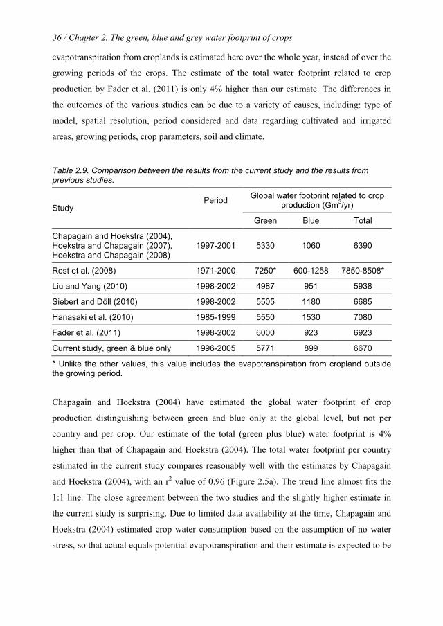
36 / Chapter 2. The green, blue and grey water footprint of crops
evapotranspiration from croplands is estimated here over the whole year, instead of over the
growing periods of the crops. The estimate of the total water footprint related to crop
production by Fader et al. (2011) is only 4% higher than our estimate. The differences in
the outcomes of the various studies can be due to a variety of causes, including: type of
model, spatial resolution, period considered and data regarding cultivated and irrigated
areas, growing periods, crop parameters, soil and climate.
Table 2.9. Comparison between the results from the current study and the results from previous studies.
Study Period Global water footprint related to crop
production (Gm3/yr)
Green Blue Total
Chapagain and Hoekstra (2004), Hoekstra and Chapagain (2007), Hoekstra and Chapagain (2008)
1997-2001 5330 1060 6390
Rost et al. (2008) 1971-2000 7250* 600-1258 7850-8508*
Liu and Yang (2010) 1998-2002 4987 951 5938
Siebert and Döll (2010) 1998-2002 5505 1180 6685
Hanasaki et al. (2010) 1985-1999 5550 1530 7080
Fader et al. (2011) 1998-2002 6000 923 6923
Current study, green & blue only 1996-2005 5771 899 6670
* Unlike the other values, this value includes the evapotranspiration from cropland outside the growing period.
Chapagain and Hoekstra (2004) have estimated the global water footprint of crop
production distinguishing between green and blue only at the global level, but not per
country and per crop. Our estimate of the total (green plus blue) water footprint is 4%
higher than that of Chapagain and Hoekstra (2004). The total water footprint per country
estimated in the current study compares reasonably well with the estimates by Chapagain
and Hoekstra (2004), with an r2 value of 0.96 (Figure 2.5a). The trend line almost fits the
1:1 line. The close agreement between the two studies and the slightly higher estimate in
the current study is surprising. Due to limited data availability at the time, Chapagain and
Hoekstra (2004) estimated crop water consumption based on the assumption of no water
stress, so that actual equals potential evapotranspiration and their estimate is expected to be
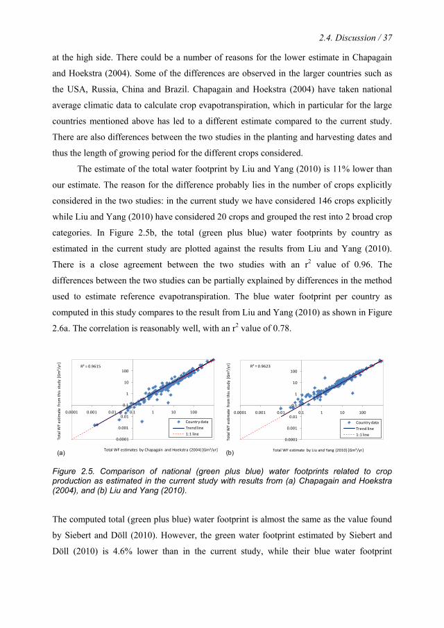
2.4. Discussion / 37
at the high side. There could be a number of reasons for the lower estimate in Chapagain
and Hoekstra (2004). Some of the differences are observed in the larger countries such as
the USA, Russia, China and Brazil. Chapagain and Hoekstra (2004) have taken national
average climatic data to calculate crop evapotranspiration, which in particular for the large
countries mentioned above has led to a different estimate compared to the current study.
There are also differences between the two studies in the planting and harvesting dates and
thus the length of growing period for the different crops considered.
The estimate of the total water footprint by Liu and Yang (2010) is 11% lower than
our estimate. The reason for the difference probably lies in the number of crops explicitly
considered in the two studies: in the current study we have considered 146 crops explicitly
while Liu and Yang (2010) have considered 20 crops and grouped the rest into 2 broad crop
categories. In Figure 2.5b, the total (green plus blue) water footprints by country as
estimated in the current study are plotted against the results from Liu and Yang (2010).
There is a close agreement between the two studies with an r2 value of 0.96. The
differences between the two studies can be partially explained by differences in the method
used to estimate reference evapotranspiration. The blue water footprint per country as
computed in this study compares to the result from Liu and Yang (2010) as shown in Figure
2.6a. The correlation is reasonably well, with an r2 value of 0.78.
R² = 0.9615
0.0001
0.001
0.01
0.1
1
10
100
0.0001 0.001 0.01 0.1 1 10 100
Tota
l WF
estim
ate
from
this
stu
dy [
Gm
3 /yr
]
Total WF estimates by Chapagain and Hoekstra (2004) [Gm3/yr]
Country dataTrend line1:1 line
R² = 0.9623
0.0001
0.001
0.01
0.1
1
10
100
0.0001 0.001 0.01 0.1 1 10 100
Tota
l WF
estim
ate
from
this
stu
dy [
Gm
3 /yr
]
Total WF estimate by Liu and Yang (2010) [Gm3/yr]
Country dataTrend line1:1 line
(a) (b)
Figure 2.5. Comparison of national (green plus blue) water footprints related to crop production as estimated in the current study with results from (a) Chapagain and Hoekstra (2004), and (b) Liu and Yang (2010).
The computed total (green plus blue) water footprint is almost the same as the value found
by Siebert and Döll (2010). However, the green water footprint estimated by Siebert and
Döll (2010) is 4.6% lower than in the current study, while their blue water footprint
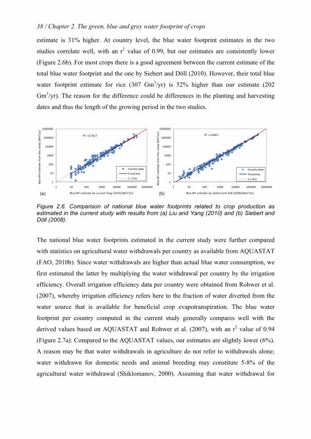
38 / Chapter 2. The green, blue and grey water footprint of crops
estimate is 31% higher. At country level, the blue water footprint estimates in the two
studies correlate well, with an r2 value of 0.99, but our estimates are consistently lower
(Figure 2.6b). For most crops there is a good agreement between the current estimate of the
total blue water footprint and the one by Siebert and Döll (2010). However, their total blue
water footprint estimate for rice (307 Gm3/yr) is 52% higher than our estimate (202
Gm3/yr). The reason for the difference could be differences in the planting and harvesting
dates and thus the length of the growing period in the two studies.
R² = 0.7827
1
10
100
1000
10000
100000
1000000
1 10 100 1000 10000 100000 1000000
Blue
WF
estim
ate
from
thi
s st
udy
[Mm
3 /yr
]
Blue WF estimate by Liu and Yang (2010) [Mm3/yr]
Country data
Trend line
1:1 line
R² = 0.9907
1
10
100
1000
10000
100000
1000000
1 10 100 1000 10000 100000 1000000
Blue
WF
estim
ate
from
thi
s st
udy
[Mm
3 /yr
]
Blue WF estimate by Siebert and Döll (2008) [Mm3/yr]
Country data
Trend line
1:1 line
(a) (b)
Figure 2.6. Comparison of national blue water footprints related to crop production as estimated in the current study with results from (a) Liu and Yang (2010) and (b) Siebert and Döll (2008).
The national blue water footprints estimated in the current study were further compared
with statistics on agricultural water withdrawals per country as available from AQUASTAT
(FAO, 2010b). Since water withdrawals are higher than actual blue water consumption, we
first estimated the latter by multiplying the water withdrawal per country by the irrigation
efficiency. Overall irrigation efficiency data per country were obtained from Rohwer et al.
(2007), whereby irrigation efficiency refers here to the fraction of water diverted from the
water source that is available for beneficial crop evapotranspiration. The blue water
footprint per country computed in the current study generally compares well with the
derived values based on AQUASTAT and Rohwer et al. (2007), with an r2 value of 0.94
(Figure 2.7a). Compared to the AQUASTAT values, our estimates are slightly lower (6%).
A reason may be that water withdrawals in agriculture do not refer to withdrawals alone;
water withdrawn for domestic needs and animal breeding may constitute 5-8% of the
agricultural water withdrawal (Shiklomanov, 2000). Assuming that water withdrawal for

2.4. Discussion / 39
irrigation equals agricultural water withdrawal may thus lead to a slight overestimation of
the blue water footprint from the statistics.
The blue water footprints estimated in the current study can also be compared with
consumptive water use in irrigation on the level of federal states in the USA. Hutson et al.
(2004) provide irrigation water withdrawal at federal state level for the year 2000.
Consumptive blue water use for the year 2000 was derived using the ratio of consumptive
water use to water withdrawal for irrigation at state level for the year 1995 (Solley et al.,
1998). Our estimated blue water footprints at federal state level correlate well with the
statistic data, at least for states with high irrigation water use. The blue water footprints at
the state level obtained in the current study, however, are generally lower than the values
obtained from the statistics (Figure 2.7b).
R² = 0.9359
1
10
100
1000
10000
100000
1000000
1 10 100 1000 10000 100000 1000000
Blue
WF
estim
ate
from
thi
s st
udy
[Mm
3 /yr
]
Blue WF estimate from AQUASTAT [Mm3/yr]
Country data
Trend line
1:1 line
R² = 0.9185
0.1
1
10
100
1000
10000
100000
0.1 1 10 100 1000 10000 100000
Blue
WF
estim
ate
from
thi
s st
udy
[Mm
3 /yr
]
Blue WF estimate from USGS [Mm3/yr]
State data
Trend line
1:1 line
(a) (b)
Figure 2.7. Comparison of blue water footprints related to crop production as estimated in the current study with results from (a) AQUASTAT (FAO, 2010b) for developing countries, and (b) USGS (Hutson et al., 2004; Solley et al., 1998) for the states in the USA.
The calculated national blue water footprints were further compared to the irrigation water
requirements for 90 developing countries as estimated by FAO (2005a) for the year 2000.
As can be seen in Figure 2.8, the calculated national blue water footprints are consistently
lower than the national irrigation requirements from FAO (2005a), which can be explained
by the use of different land use data and differences in model set-up in the two studies. In
the current study, the soil water balance was made on a daily basis while in FAO (2005a)
the soil water balance was done with a monthly time step. Besides, for rice irrigation water
requirements, FAO (2005a) added an additional 250 mm of water to flood the paddy fields.
The water footprint per ton of crop has been compared with results from Chapagain
and Hoekstra (2004) and Siebert and Döll (2010). The global average water footprint per
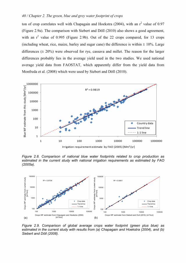
40 / Chapter 2. The green, blue and grey water footprint of crops
ton of crop correlates well with Chapagain and Hoekstra (2004), with an r2 value of 0.97
(Figure 2.9a). The comparison with Siebert and Döll (2010) also shows a good agreement,
with an r2 value of 0.995 (Figure 2.9b). Out of the 22 crops compared, for 13 crops
(including wheat, rice, maize, barley and sugar cane) the difference is within ± 10%. Large
differences (± 20%) were observed for rye, cassava and millet. The reason for the larger
differences probably lies in the average yield used in the two studies. We used national
average yield data from FAOSTAT, which apparently differ from the yield data from
Monfreda et al. (2008) which were used by Siebert and Döll (2010).
R² = 0.9819
1
10
100
1000
10000
100000
1000000
1 10 100 1000 10000 100000 1000000
Blue
WF
estim
ate
from
thi
s st
udy
[Mm
3 /yr]
Irrigation requirement estimate by FAO (2005) [Mm3/yr]
Country data
Trend line
1:1 line
Figure 2.8. Comparison of national blue water footprints related to crop production as estimated in the current study with national irrigation requirements as estimated by FAO (2005a).
R² = 0.9951
100
1000
10000
100000
100 1000 10000 100000
Cro
ps W
F es
timat
e fr
om c
urre
nt s
tudy
[m
3 /to
n]
Crops WF estimate f rom Siebert and Doll (2010) [m3/ton]
Crop dataTrend line1:1 line
R² = 0.9709
100
1000
10000
100000
100 1000 10000 100000
Cro
ps W
F es
timat
e fr
om c
urre
nt s
tudy
[m
3 /to
n]
Crops WF estimate f rom Chapagain and Hoekstra (2004) [m3/ton]
Crop dataTrend line1:1 line
(a) (b)
Figure 2.9. Comparison of global average crops water footprint (green plus blue) as estimated in the current study with results from (a) Chapagain and Hoekstra (2004), and (b) Siebert and Döll (2008).

2.5. Conclusion / 41
Since all studies depend on a large set of assumptions with respect to modelling structure,
parameter values and datasets used, as it was already pointed out by Mekonnen and
Hoekstra (2010a), it is difficult to attribute differences in estimates from the various studies
to specific factors; also it is difficult to assess the quality of our new estimates relative to
the quality of earlier estimates. The quality of data used defines the accuracy of the model
output. All studies suffer the same sorts of limitations in terms of data availability and
quality and deal with that in different ways. In future studies it would be useful to spend
more effort in studying the sensitivity of the model outcomes to assumptions and
parameters and assessing the uncertainties in the final outcome.
2.5 Conclusion
The study shows that the global water footprint of crop production for the period 1996-
2005 was 7404 Gm3/yr. The large fraction of green water (78%) confirms the importance of
green water in global food production. The fraction of blue water is smaller (12%), but as
the spatial analysis shows, the regions where blue water footprints are large are often arid
and semi-arid regions where water scarcity is high. The share of the grey water footprint is
relatively small as well (10%), but this is a conservative estimate, because we have
analysed the required assimilation volume for leached nitrogen fertilizers only, leaving out
relevant pollutants such as phosphorus and pesticides.
The finding in this study agrees with earlier studies that green water plays a
prominent role in the global crop production. As shown by Rockström et al. (2009), most
countries in theory have a green water based self-sufficiency potential and are in a position
to produce their entire food requirement locally. Rockström et al. (2003) showed that there
is great opportunity to improve water productivity through improving yield levels as much
as four folds within the available water balance in rain-fed agriculture. This offers a good
opportunity to increase food production from rain-fed agriculture by raising water
productivity without requiring additional blue water resources (Critchely and Siegert, 1991;
Rockström and Barron, 2007; Rockström et al., 2003, 2007a, 2007b). However, the
marginal benefit of additional blue water in semi-arid and arid regions is quite large in
terms of raising productivity. Globally, the current cereal production would be significantly
lower if no blue water is applied (Hoff et al., 2010; Rost et al., 2009; Siebert and Döll,
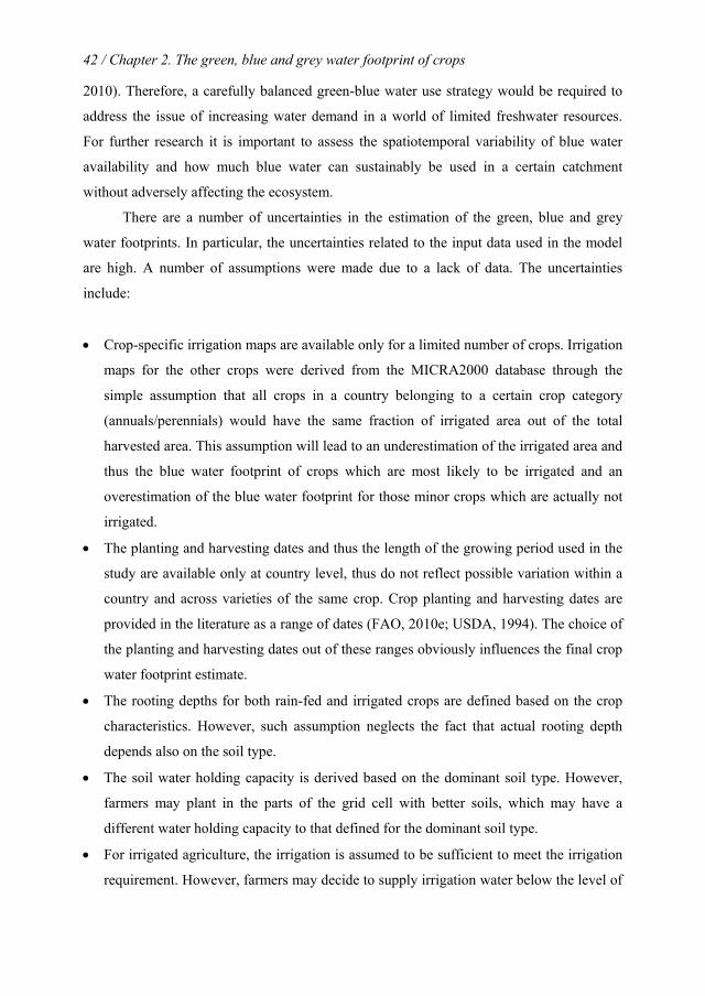
42 / Chapter 2. The green, blue and grey water footprint of crops
2010). Therefore, a carefully balanced green-blue water use strategy would be required to
address the issue of increasing water demand in a world of limited freshwater resources.
For further research it is important to assess the spatiotemporal variability of blue water
availability and how much blue water can sustainably be used in a certain catchment
without adversely affecting the ecosystem.
There are a number of uncertainties in the estimation of the green, blue and grey
water footprints. In particular, the uncertainties related to the input data used in the model
are high. A number of assumptions were made due to a lack of data. The uncertainties
include:
• Crop-specific irrigation maps are available only for a limited number of crops. Irrigation
maps for the other crops were derived from the MICRA2000 database through the
simple assumption that all crops in a country belonging to a certain crop category
(annuals/perennials) would have the same fraction of irrigated area out of the total
harvested area. This assumption will lead to an underestimation of the irrigated area and
thus the blue water footprint of crops which are most likely to be irrigated and an
overestimation of the blue water footprint for those minor crops which are actually not
irrigated.
• The planting and harvesting dates and thus the length of the growing period used in the
study are available only at country level, thus do not reflect possible variation within a
country and across varieties of the same crop. Crop planting and harvesting dates are
provided in the literature as a range of dates (FAO, 2010e; USDA, 1994). The choice of
the planting and harvesting dates out of these ranges obviously influences the final crop
water footprint estimate.
• The rooting depths for both rain-fed and irrigated crops are defined based on the crop
characteristics. However, such assumption neglects the fact that actual rooting depth
depends also on the soil type.
• The soil water holding capacity is derived based on the dominant soil type. However,
farmers may plant in the parts of the grid cell with better soils, which may have a
different water holding capacity to that defined for the dominant soil type.
• For irrigated agriculture, the irrigation is assumed to be sufficient to meet the irrigation
requirement. However, farmers may decide to supply irrigation water below the level of
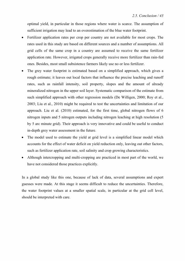
2.5. Conclusion / 43
optimal yield, in particular in those regions where water is scarce. The assumption of
sufficient irrigation may lead to an overestimation of the blue water footprint.
• Fertilizer application rates per crop per country are not available for most crops. The
rates used in this study are based on different sources and a number of assumptions. All
grid cells of the same crop in a country are assumed to receive the same fertilizer
application rate. However, irrigated crops generally receive more fertilizer than rain-fed
ones. Besides, most small subsistence farmers likely use no or less fertilizer.
• The grey water footprint is estimated based on a simplified approach, which gives a
rough estimate; it leaves out local factors that influence the precise leaching and runoff
rates, such as rainfall intensity, soil property, slopes and the amount of already
mineralized nitrogen in the upper soil layer. Systematic comparison of the estimate from
such simplified approach with other regression models (De Willigen, 2000; Roy et al.,
2003; Liu et al., 2010) might be required to test the uncertainties and limitation of our
approach. Liu et al. (2010) estimated, for the first time, global nitrogen flows of 6
nitrogen inputs and 5 nitrogen outputs including nitrogen leaching at high resolution (5
by 5 arc minute grid). Their approach is very innovative and could be useful to conduct
in-depth grey water assessment in the future.
• The model used to estimate the yield at grid level is a simplified linear model which
accounts for the effect of water deficit on yield reduction only, leaving out other factors,
such as fertilizer application rate, soil salinity and crop growing characteristics.
• Although intercropping and multi-cropping are practiced in most part of the world, we
have not considered those practices explicitly.
In a global study like this one, because of lack of data, several assumptions and expert
guesses were made. At this stage it seems difficult to reduce the uncertainties. Therefore,
the water footprint values at a smaller spatial scale, in particular at the grid cell level,
should be interpreted with care.

3. The green, blue and grey water footprint of farm animals and animal products2
Abstract The projected increase in the production and consumption of animal products is likely to
put further pressure on the globe’s freshwater resources. This paper provides a
comprehensive account of the global green, blue and grey water footprints of different sorts
of farm animals and animal products, distinguishing between different production systems
(grazing, mixed and industrial) and considering the conditions in all countries of the world
separately. The result shows that: The blue and grey water footprints of animal products are
largest for industrial systems (with an exception for chicken products). From a freshwater
perspective, animal products from grazing systems are therefore to be preferred above
products from industrial systems; The water footprint of any animal product is larger than
the water footprint of a wisely chosen crop product with equivalent nutritional value; 29%
of the total water footprint of the agricultural sector in the world is related to the production
of animal products. One third of the global water footprint of animal production is related
to beef cattle.
3.1 Introduction
The global meat production has almost doubled in the period 1980-2004 (FAO, 2005b) and
this trend is likely to continue given the projected doubling of meat production in the period
2000-2050 (Steinfeld et al., 2006). To meet this rising demand for animal products, the on-
going shift from traditional extensive and mixed farming to industrial farming systems is
likely to continue (Bouwman et al., 2005, Naylor et al., 2005, Galloway et al., 2007). There
is a rich literature on the expected environmental consequences of increased consumption
of animal products (Naylor et al., 2005; Myers and Kent, 2003; McAlpine et al., 2009;
Pelletier and Tyedmers, 2010; Sutton et al., 2011) and on the pros and cons of industrial
versus conventional farming systems (Lewis and others 1990; Capper et al., 2009). Specific
fields of interest include, amongst others, animal welfare (Fraser, 2008; Thompson, 2008),
2 Based on Mekonnen and Hoekstra (2010e)
46 / Chapter 3. The green, blue and grey water footprint of animal products
excessive use of antibiotics (Gustafson and Bowen, 1997; Witte, 1998; Smith et al., 2002;
McEwen, 2006), the demand for scarce lands to produce the required feed (Naylor et al.,
2005; Keyzer et al., 2005; Nepstad et al., 2006) and the contribution of livestock to the
emission of greenhouse gases (Pelletier and Tyedmers, 2010; Tilman et al., 2001;
Bouwman et al., 2011). Although it is known that animal products are very water intensive
(Pimentel et al., 2004; Chapagain and Hoekstra, 2003), little attention has been paid thus far
to the total impact of the livestock sector on the global demand for freshwater resources.
Because of the larger dependence on concentrate feed in industrial systems, the
intensification of animal production systems will result in increasing blue and grey water
footprints per unit of animal product. The pressure on the global freshwater resources will
thus increase both because of the increasing meat consumption and the increasing blue and
grey water footprint per unit of meat consumed.
As a result of the increasing global trade in feed crops and animal products and the
growth of meat preservation over longer periods, consumers of animal products are
spatially disconnected from the processes necessary to produce the products (Naylor et al.,
2005; Hoekstra, 2010). The concept of ‘water footprint’ provides an appropriate framework
of analysis to find the link between the consumption of animal products and the use of the
global water resources. The water footprint is defined as the total volume of freshwater that
is used to produce the goods and services consumed by an individual or community
(Hoekstra and Chapagain, 2008). The blue water footprint refers to the volume of surface
and groundwater consumed (evaporated) as a result of the production of a good; the green
water footprint refers to the rainwater consumed. The grey water footprint of a product
refers to the volume of freshwater that is required to assimilate the load of pollutants based
on existing ambient water quality standards.
There are a few earlier publications on water use in animal production. The first and
most comprehensive assessment of the water footprint of farm animals and animal products
was carried out by Chapagain and Hoekstra (2003) and later updated by the same authors in
their water footprint of nation’s publication (Chapagain and Hoekstra, 2004). A study by
FAO has quantified the global blue water use for feed production, animal drinking and
servicing (Steinfeld et al., 2006). De Fraiture et al. (2007) have estimated the global water
use for animal feed production, both green and blue but not distinguishing between the two.
Galloway et al. (2007) produced a study on the water consumption for chicken and pig for
3.1. Introduction / 47
four countries. Peden et al. (2007) made an estimate of the global water consumption for
producing the feed for farm animals. In addition to the studies mentioned there have been a
few more specific studies for the Nile River Basin (Van Breugel et al., 2010) and for the
USA (Renault and Wallender, 2000; Pimentel et al., 2004).
With the exception of Chapagain and Hoekstra (2003, 2004), none of the studies
have estimated the water footprint of animal products by product and country at a global
level. Although Chapagain and Hoekstra (2003, 2004) were able to estimate the water
footprint of farm animals and animal products per country, they have taken a very crude
assumption on the composition and amount of feed consumed by the different animals.
Besides, the water footprints of feed crops were estimated based on national average
climatic data. We have tried to improve the estimation of feed composition and feed
amount per animal category and have used better estimates for the water footprints of feed
crops:
• We have estimated the amount of feed consumed per animal category, per production
system and per country based on estimates of feed conversion efficiencies and statistics
on the annual production of animal products. Chapagain and Hoekstra (2003, 2004)
have taken rough assumptions on the quantities of feed consumed per animal category
based on incidental data.
• We reckon with the relative occurrence of the three production systems (grazing, mixed
and industrial) in each country, using the studies of Seré and Steinfeld (1996) and Wint
and Robinson (2007).
• We have estimated the green, blue and grey water footprints of the feed crops using a
spatially explicit crop water use model able to estimate actual crop water use
(Mekonnen and Hoekstra, 2010a, 2010d).
The objective of the study is to assess the water footprint of farm animals and the various
derived animal products per animal production systems for the period 1996-2005. We
consider eight animal categories: beef and dairy cattle, pig, sheep, goat, broiler and layer
chicken and horses.
48 / Chapter 3. The green, blue and grey water footprint of animal products
3.2 Method
We follow the water footprint definitions and methodology as set out in Hoekstra et al.
(2009). The blue water footprint refers to consumption of blue water resources (surface and
groundwater) along the supply chain of a product. ‘Consumption’ refers to loss of water
from the available ground-surface water body in a catchment area. Losses occur when
water evaporates, returns to another catchment area or the sea or is incorporated into a
product. The green water footprint refers to consumption of green water resources
(rainwater in so far as it does not become run-off). The grey water footprint refers to
pollution and is defined as the volume of freshwater that is required to assimilate the load
of pollutants given natural background concentrations and existing ambient water quality
standards.
We consider eight farm animal categories: beef and dairy cattle, pig, sheep, goat,
broiler and layer chicken and horses. When estimating total feed amounts and total water
footprints per category, we include ‘buffaloes’ in the category of ‘beef cattle’ and ‘asses
and mules’ in the category of ‘horses’.
The water footprint of a live animal consists of different components: the indirect
water footprint of the feed and the direct water footprint related to the drinking water and
service water consumed (Chapagain and Hoekstra, 2003, 2004). The water footprint of an
animal is expressed as:
],,[],,[],,[],,[ scaWFscaWFscaWFscaWF servdrinkfeed ++= (4)
where WFfeed[a,c,s], WFdrink[a,c,s] and WFserv[a,c,s] represent the water footprint of an
animal for animal category a in country c in production systems s related to feed, drinking
water and service water consumption, respectively. Service water refers to the water used to
clean the farmyard, wash the animal and carry out other services necessary to maintain the
environment. The water footprint of an animal and its three components can be expressed
in terms of m3/yr/animal, or, when summed over the lifetime of the animal, in terms of
m3/animal. For beef cattle, pig, sheep, goat and broiler chicken – animals that provide their
products after they have been slaughtered – it is most useful to look at the water footprint of
the animal at the end of its lifetime, because it is this total that will be allocated to the
3.2. Method / 49
various products (e.g. meat, leather). For dairy cattle and layer chicken, it is most
straightforward to look at the water footprint of the animal per year (averaged over its
lifetime), because one can easily relate this annual animal water footprint to its average
annual production (milk, eggs).
The water footprint of an animal related to the feed consumed consists of two parts:
the water footprint of the various feed ingredients and the water that is used to mix the feed:
( )],,[
],,[][],,,[
],,[ 1
scaPop
scaWFpWFpscaFeed
scaWF
n
pmixingprod
feed ∗=
∗∑ +×
= (5)
Feed[a,c,s,p] represents the annual amount of feed ingredient p consumed by animal
category a in country c and production system s (ton/yr), ]p[WFprod∗ the water footprint of
feed ingredient p (m3/ton), WFmixing[a,c,s] the volume of water consumed for mixing the
feed for animal category a in country c and production system s (m3/yr/animal) and
Pop*[a,c,s] the number of slaughtered animals per year or the number of milk or egg
producing animals in a year for animal category a in country c and production system s.
The water footprint of feed ingredients
The water footprints of the different crops, roughages and crop by-products ( ][ pWFprod∗ ,
m3/ton) that are eaten by the various farm animals have been calculated following the
methodology developed by Hoekstra and Chapagain (2008) and Hoekstra et al. (2009). The
water footprints of feed crops were estimated using a crop water use model that estimates
crop water footprints at a 5 by 5 arc minute spatial resolution globally (Mekonnen and
Hoekstra, 2010a, 2010d). Grey water footprints were estimated by looking at leaching and
runoff of nitrogen fertilisers only, following Mekonnen and Hoekstra (2010a,d). Since
animal feed in a country originates from domestic production and imported products, for
the calculation of the water footprint of animal feed in a country, we have taken a weighted
average water footprint according to the relative volumes of domestic production and
import:
50 / Chapter 3. The green, blue and grey water footprint of animal products
( )
∑∑+
×+×
=∗
e
e
nei
neprodeiprod
prod ,pnTpP
,pnWF,pnTpWFpP
pWF][][
][][][][
][ (6)
in which P[p] is the production quantity of feed product p in a country (ton/yr), Ti[ne,p] the
imported quantity of feed product p from exporting nation ne (ton/yr), WFprod[p] the water
footprint of feed product p when produced in the nation considered (m3/ton) and
WFprod[ne,p] the water footprint of feed product p as in the exporting nation ne (m3/ton). The
water footprint of crop residues such as bran, straw, chaff and leaves and tops from sugar
beet have already been accounted for in the main product, therefore their water footprint
was set equal to zero.
Volume and composition of feed
The volume and composition of the feed consumed vary depending on the type of animal,
the production system and the country. The amount of feed consumed is estimated
following the approach of Hendy et al. (1995), in which the total annual feed consumption
(including both concentrates and roughages) is calculated based on annual production of
animal products and feed conversion efficiencies. Only for horses we have used the
approach as in Chapagain and Hoekstra (2003), which means that we multiplied the
estimated feed consumption per animal by the number of animals, thus arriving at an
estimate of the total feed consumed by horses.
The total feed per production system for both ruminants and non-ruminants animals is
calculated as follows:
]s,c,a[P]s,c,a[FCE]s,c,a[Feed ×= (7)
where Feed[a,c,s] is the total amount of feed consumed by animal category a (ton/yr) in
country c and production system s, FCE[a,c,s] the feed conversion efficiency (kg dry mass
of feed / kg of product) for animal category a in country c and production system s, and

3.2. Method / 51
P[a,c,s] the total amount of product (meat, milk, or egg) produced by animal category a
(ton/yr) in country c and production system s.
Estimating feed conversion efficiencies
Feed conversion efficiency is defined as the amount of feed consumed per unit of produced
animal product (e.g. meat, milk, egg). Feed conversion efficiencies were estimated
separately for each animal category (beef cattle, dairy cattle, sheep, goat, pig, broiler
chicken and egg layer chicken), for each animal production system and per country.
Although the term used may suggest precisely the opposite, animals that have a low ‘feed
conversion efficiency’ are efficient users of feed. We use the term here as generally used in
livestock studies. The feed conversion efficiencies (FCE, kg dry mass/kg product) for non-
ruminants (pig and chicken) were adopted from Hendy et al. (1995). For ruminants (cattle,
goat, sheep), feed conversion efficiencies were estimated through dividing feed intake per
capita by annual production (of beef, milk, sheep and goat meat) per capita:
],,[],,[],,[
scaPOscaFIscaFCE = (8)
where FI[a,c,s] is the feed intake per head by ruminant animal category a in country c and
production system s (kg dry mass/yr/animal), and PO[a,c,s] the product output per head for
ruminant animal category a in country c and production system s (kg product/yr/animal).
The product output (beef, milk, sheep and goat meat) per animal for ruminants is calculated
as:
],,[],,[],,[scaPop
scaPscaPO = (9)
in which P[a,c,s] is the total annual production of beef, milk, sheep meat or goat meat in
country c in production system s (kg/yr) and Pop[a,c,s] the total population of beef cattle,
dairy cattle, sheep or goat in that country and production system.
52 / Chapter 3. The green, blue and grey water footprint of animal products
Estimating the total annual production of animal products
The meat production (Pmeat, ton/yr) per animal category a (beef cattle, pig, sheep and goat)
in country c and production system s is estimated by multiplying the carcass yield per
slaughtered animal by the annual number of animals slaughtered:
],,[],,[],,[ scaSAscaCYscaPmeat ×= (10)
The carcass yield (CY, kg/animal) for each animal category per production system was
estimated by combining country average carcass yield data from FAO (2010a) with data on
animal live weight per production system per economic region (Hendy et al. 1995) and data
on carcass weight as percentage of live weight (FAO, 2003). The obtained carcass yields
were scaled such that the total meat production per animal category equals the value
provided by FAO (2010a). The number of slaughtered animals per production system (SA,
number of animal/yr) was calculated by multiplying the total animal number by the animal
off-take rate per production system:
],,[],,[],,[ scaORscaPopscaSA ×= (11)
where Pop[a,c,s] is the population of animal category a in country c for production system
s and OR[a,c,s] the off-take rate, which is the fraction of the animal population that is taken
out in a given year for slaughter (dimensionless).
Milk and egg production per production system and country were calculated as:
],,[],,[],,[ scaDCscaMYscaPmilk ×= (12)
],[],,[],,[ caPscafscaP eggeggegg ×= (13)
where Pmilk[a,c,s] and Pegg[a,c,s] represent production of milk and egg in country c and
production system s respectively (ton/yr), MY[a,c,s] milk yield per dairy cow in country c
and production system s (ton/dairy cow), DC[a,c,s] the number of dairy cows in country c

3.2. Method / 53
and production system s, fegg[a,c,s] the fraction of egg produced in country c and production
system s and Pegg[a,c] the total amount of egg produced in country c (ton/yr).
Estimating the feed composition
Animal feeds are generally divided into ‘concentrates’ and ‘roughages’. The volume of
concentrate feed has been estimated per animal category and per production system as:
],,[],,[],,[ scafscaFeedscaeConcentrat c×= (14)
where Concentrate[a,c,s] is the volume of concentrate feed consumed by animal category a
in country c and production system s (ton/yr) and fc[a,c,s] the fraction of concentrate in the
total feed for animal category a in country c and production system s. For the latter
variable, data have been obtained from Hendy et al. (1995) and Bouwman et al. (2005).
The composition of concentrate feeds varies across animal species and regions of the world.
To our knowledge, there are no datasets with global coverage on the composition of feed
for the different animals per country. Therefore, we have made a number of assumptions
concerning the concentrate feed composition of the different animal species. According to
Hendy et al. (1995), the diets of pig and poultry include, on average, 50-60% cereals, 10-
20% oil meals and 15-25% ‘other concentrates’ (grain substitutes, milling by-products,
non-conventional concentrates). Wheeler et al. (1981) provide the feed composition in
terms of major crop categories for the different animal categories. We have used these and
other sources in combination with FAOSTAT country average concentrate feed values for
the period 1996-2003 (FAO, 2010a) to estimate the diet composition of the different animal
species. In order to estimate the feed in terms of specific crops per animal, we first
estimated the feed in terms of major crop categories following Wheeler et al. (1981). The
feed in terms of major crop categories is further distributed to each crop proportional to the
crop’s share in its crops category as obtained from FAOSTAT (FAO, 2010a). The roughage
feed is divided into fodder, grass and crop residues using the data obtained from Bouwman
et al. (2005).
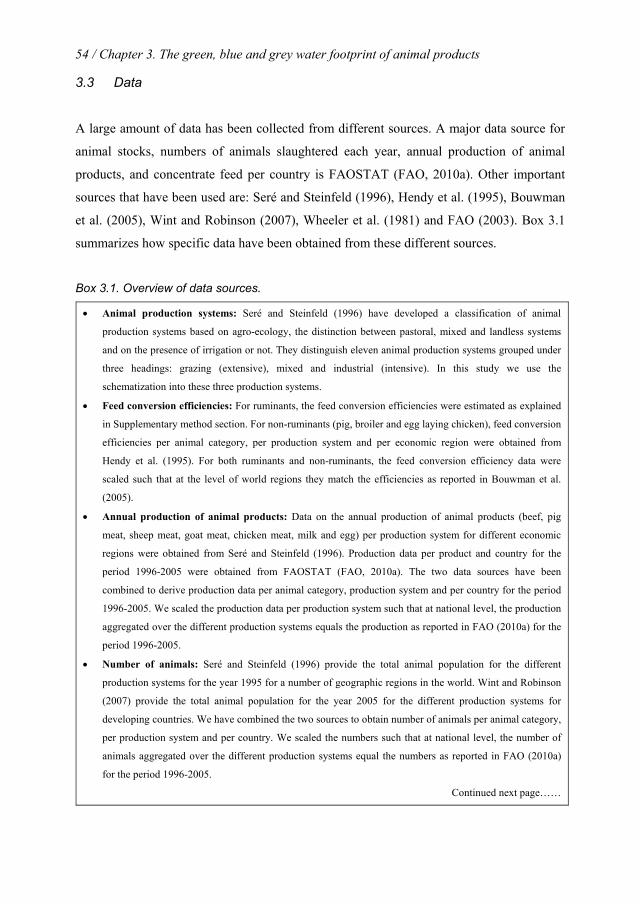
54 / Chapter 3. The green, blue and grey water footprint of animal products
3.3 Data
A large amount of data has been collected from different sources. A major data source for
animal stocks, numbers of animals slaughtered each year, annual production of animal
products, and concentrate feed per country is FAOSTAT (FAO, 2010a). Other important
sources that have been used are: Seré and Steinfeld (1996), Hendy et al. (1995), Bouwman
et al. (2005), Wint and Robinson (2007), Wheeler et al. (1981) and FAO (2003). Box 3.1
summarizes how specific data have been obtained from these different sources.
Box 3.1. Overview of data sources.
• Animal production systems: Seré and Steinfeld (1996) have developed a classification of animal
production systems based on agro-ecology, the distinction between pastoral, mixed and landless systems
and on the presence of irrigation or not. They distinguish eleven animal production systems grouped under
three headings: grazing (extensive), mixed and industrial (intensive). In this study we use the
schematization into these three production systems.
• Feed conversion efficiencies: For ruminants, the feed conversion efficiencies were estimated as explained
in Supplementary method section. For non-ruminants (pig, broiler and egg laying chicken), feed conversion
efficiencies per animal category, per production system and per economic region were obtained from
Hendy et al. (1995). For both ruminants and non-ruminants, the feed conversion efficiency data were
scaled such that at the level of world regions they match the efficiencies as reported in Bouwman et al.
(2005).
• Annual production of animal products: Data on the annual production of animal products (beef, pig
meat, sheep meat, goat meat, chicken meat, milk and egg) per production system for different economic
regions were obtained from Seré and Steinfeld (1996). Production data per product and country for the
period 1996-2005 were obtained from FAOSTAT (FAO, 2010a). The two data sources have been
combined to derive production data per animal category, production system and per country for the period
1996-2005. We scaled the production data per production system such that at national level, the production
aggregated over the different production systems equals the production as reported in FAO (2010a) for the
period 1996-2005.
• Number of animals: Seré and Steinfeld (1996) provide the total animal population for the different
production systems for the year 1995 for a number of geographic regions in the world. Wint and Robinson
(2007) provide the total animal population for the year 2005 for the different production systems for
developing countries. We have combined the two sources to obtain number of animals per animal category,
per production system and per country. We scaled the numbers such that at national level, the number of
animals aggregated over the different production systems equal the numbers as reported in FAO (2010a)
for the period 1996-2005.
Continued next page……
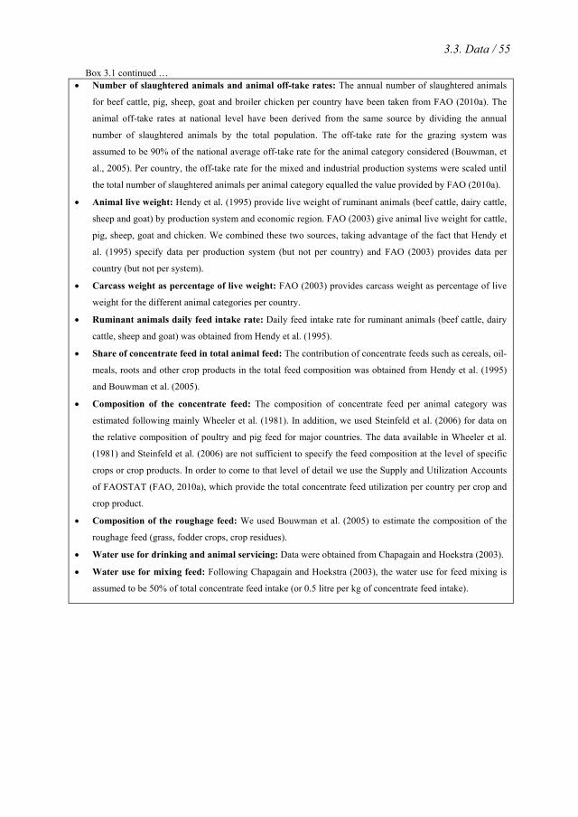
3.3. Data / 55
Box 3.1 continued … • Number of slaughtered animals and animal off-take rates: The annual number of slaughtered animals
for beef cattle, pig, sheep, goat and broiler chicken per country have been taken from FAO (2010a). The
animal off-take rates at national level have been derived from the same source by dividing the annual
number of slaughtered animals by the total population. The off-take rate for the grazing system was
assumed to be 90% of the national average off-take rate for the animal category considered (Bouwman, et
al., 2005). Per country, the off-take rate for the mixed and industrial production systems were scaled until
the total number of slaughtered animals per animal category equalled the value provided by FAO (2010a).
• Animal live weight: Hendy et al. (1995) provide live weight of ruminant animals (beef cattle, dairy cattle,
sheep and goat) by production system and economic region. FAO (2003) give animal live weight for cattle,
pig, sheep, goat and chicken. We combined these two sources, taking advantage of the fact that Hendy et
al. (1995) specify data per production system (but not per country) and FAO (2003) provides data per
country (but not per system).
• Carcass weight as percentage of live weight: FAO (2003) provides carcass weight as percentage of live
weight for the different animal categories per country.
• Ruminant animals daily feed intake rate: Daily feed intake rate for ruminant animals (beef cattle, dairy
cattle, sheep and goat) was obtained from Hendy et al. (1995).
• Share of concentrate feed in total animal feed: The contribution of concentrate feeds such as cereals, oil-
meals, roots and other crop products in the total feed composition was obtained from Hendy et al. (1995)
and Bouwman et al. (2005).
• Composition of the concentrate feed: The composition of concentrate feed per animal category was
estimated following mainly Wheeler et al. (1981). In addition, we used Steinfeld et al. (2006) for data on
the relative composition of poultry and pig feed for major countries. The data available in Wheeler et al.
(1981) and Steinfeld et al. (2006) are not sufficient to specify the feed composition at the level of specific
crops or crop products. In order to come to that level of detail we use the Supply and Utilization Accounts
of FAOSTAT (FAO, 2010a), which provide the total concentrate feed utilization per country per crop and
crop product.
• Composition of the roughage feed: We used Bouwman et al. (2005) to estimate the composition of the
roughage feed (grass, fodder crops, crop residues).
• Water use for drinking and animal servicing: Data were obtained from Chapagain and Hoekstra (2003).
• Water use for mixing feed: Following Chapagain and Hoekstra (2003), the water use for feed mixing is
assumed to be 50% of total concentrate feed intake (or 0.5 litre per kg of concentrate feed intake).

56 / Chapter 3. The green, blue and grey water footprint of animal products
3.4 Results
3.4.1 Quantity and composition of animal feed
Table 3.1 provides global average feed conversion efficiencies for different animal
categories and production systems. Ruminants (cattle, sheep, goat) are less efficient in
converting feed into meat than non-ruminants (pig, chicken), amongst other due to the
lower quality of feed they consume. Particularly meat production from cattle costs a lot of
feed per unit of product obtained. Although ruminants need more feed, their feed largely
consists of forage and other materials that humans cannot eat, while non-ruminants
consume large amounts of concentrate feed that could be used for human consumption.
Non-ruminants thus most obviously compete with humans for food, but in an indirect way
ruminants also compete for food with humans. In some cases the roughages eaten by
ruminants are produced with land and water resources that cannot alternatively be allocated
to crop production for human consumption (e.g. in the case of grazing in dry or wetlands),
but often the land and water resources used for roughages supply can alternatively be used
for crop growth for human consumption, so that ruminants compete with humans for food
also through consumption of roughages.
Table 3.1. Global average feed conversion efficiency per animal category and production system.
Animal category Feed conversion efficiency (kg dry mass feed/kg output)
Grazing Mixed Industrial Overall
Beef cattle 70.1 51.8 19.2 46.9
Dairy cattle 3.5 1.6 1.1 1.9
Broiler chicken 9.0 4.9 2.8 4.2
Layer chicken 9.3 4.4 2.3 3.1
Pig 11.3 6.5 3.9 5.8
Sheep and goat 49.6 25.8 13.3 30.2
Non-ruminants are responsible for 60% of the global consumption of concentrate feeds;
ruminants account for 40%. Figure 3.1 shows the consumption of different concentrates by
different animal categories. Chickens take the largest share in total concentrate feed
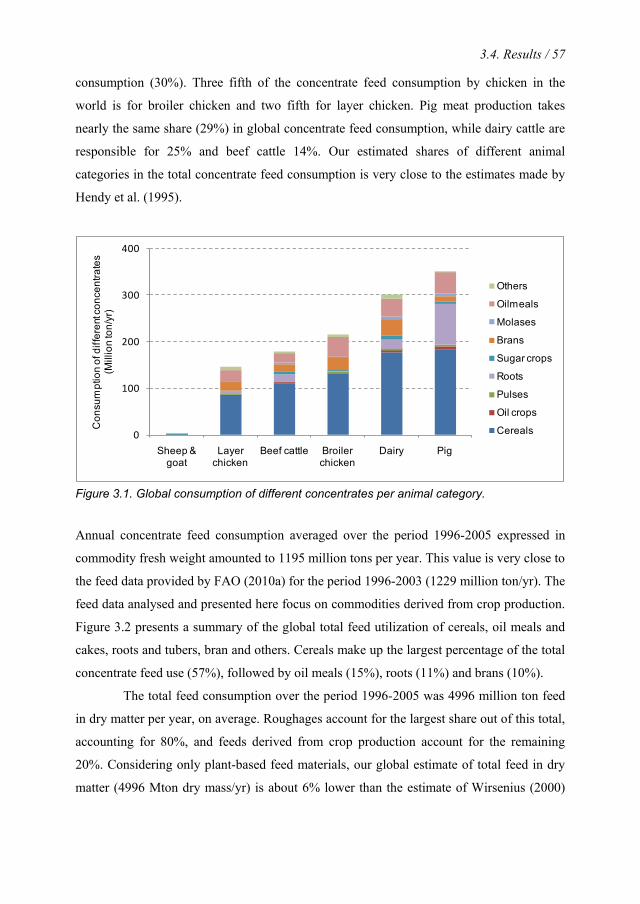
3.4. Results / 57
consumption (30%). Three fifth of the concentrate feed consumption by chicken in the
world is for broiler chicken and two fifth for layer chicken. Pig meat production takes
nearly the same share (29%) in global concentrate feed consumption, while dairy cattle are
responsible for 25% and beef cattle 14%. Our estimated shares of different animal
categories in the total concentrate feed consumption is very close to the estimates made by
Hendy et al. (1995).
0
100
200
300
400
Sheep & goat
Layer chicken
Beef cattle Broiler chicken
Dairy Pig
Con
sum
ptio
n of
diff
eren
t con
cent
rate
s (M
illio
n to
n/yr
)
Others
Oilmeals
Molases
Brans
Sugar crops
Roots
Pulses
Oil crops
Cereals
Figure 3.1. Global consumption of different concentrates per animal category.
Annual concentrate feed consumption averaged over the period 1996-2005 expressed in
commodity fresh weight amounted to 1195 million tons per year. This value is very close to
the feed data provided by FAO (2010a) for the period 1996-2003 (1229 million ton/yr). The
feed data analysed and presented here focus on commodities derived from crop production.
Figure 3.2 presents a summary of the global total feed utilization of cereals, oil meals and
cakes, roots and tubers, bran and others. Cereals make up the largest percentage of the total
concentrate feed use (57%), followed by oil meals (15%), roots (11%) and brans (10%).
The total feed consumption over the period 1996-2005 was 4996 million ton feed
in dry matter per year, on average. Roughages account for the largest share out of this total,
accounting for 80%, and feeds derived from crop production account for the remaining
20%. Considering only plant-based feed materials, our global estimate of total feed in dry
matter (4996 Mton dry mass/yr) is about 6% lower than the estimate of Wirsenius (2000)
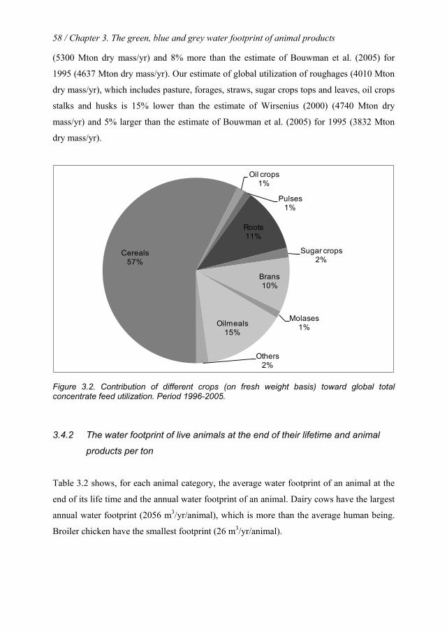
58 / Chapter 3. The green, blue and grey water footprint of animal products
(5300 Mton dry mass/yr) and 8% more than the estimate of Bouwman et al. (2005) for
1995 (4637 Mton dry mass/yr). Our estimate of global utilization of roughages (4010 Mton
dry mass/yr), which includes pasture, forages, straws, sugar crops tops and leaves, oil crops
stalks and husks is 15% lower than the estimate of Wirsenius (2000) (4740 Mton dry
mass/yr) and 5% larger than the estimate of Bouwman et al. (2005) for 1995 (3832 Mton
dry mass/yr).
Cereals57%
Oil crops1%
Pulses1%
Roots 11%
Sugar crops2%
Brans10%
Molases1%Oilmeals
15%
Others2%
Figure 3.2. Contribution of different crops (on fresh weight basis) toward global total concentrate feed utilization. Period 1996-2005.
3.4.2 The water footprint of live animals at the end of their lifetime and animal
products per ton
Table 3.2 shows, for each animal category, the average water footprint of an animal at the
end of its life time and the annual water footprint of an animal. Dairy cows have the largest
annual water footprint (2056 m3/yr/animal), which is more than the average human being.
Broiler chicken have the smallest footprint (26 m3/yr/animal).
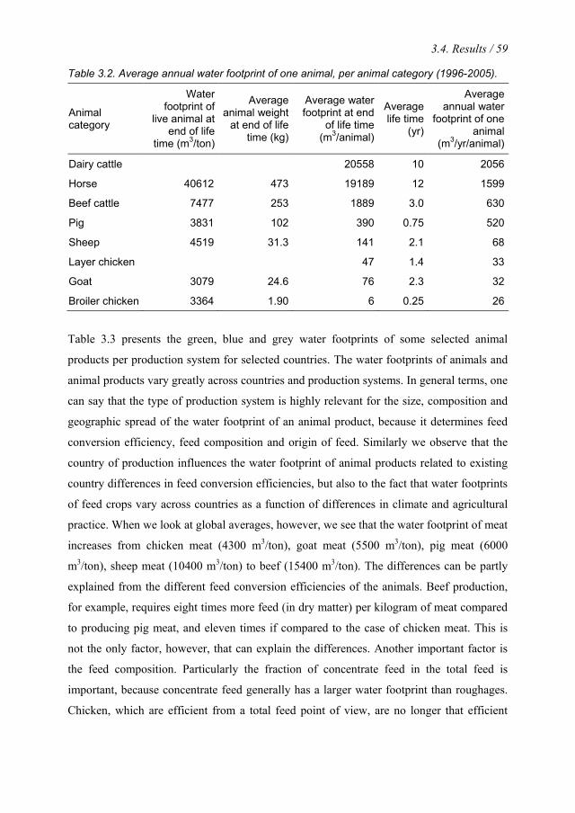
3.4. Results / 59
Table 3.2. Average annual water footprint of one animal, per animal category (1996-2005).
Animal category
Water footprint of
live animal at end of life
time (m3/ton)
Average animal weight
at end of life time (kg)
Average water footprint at end
of life time (m3/animal)
Average life time
(yr)
Average annual water
footprint of one animal
(m3/yr/animal)
Dairy cattle 20558 10 2056
Horse 40612 473 19189 12 1599
Beef cattle 7477 253 1889 3.0 630
Pig 3831 102 390 0.75 520
Sheep 4519 31.3 141 2.1 68
Layer chicken 47 1.4 33
Goat 3079 24.6 76 2.3 32
Broiler chicken 3364 1.90 6 0.25 26
Table 3.3 presents the green, blue and grey water footprints of some selected animal
products per production system for selected countries. The water footprints of animals and
animal products vary greatly across countries and production systems. In general terms, one
can say that the type of production system is highly relevant for the size, composition and
geographic spread of the water footprint of an animal product, because it determines feed
conversion efficiency, feed composition and origin of feed. Similarly we observe that the
country of production influences the water footprint of animal products related to existing
country differences in feed conversion efficiencies, but also to the fact that water footprints
of feed crops vary across countries as a function of differences in climate and agricultural
practice. When we look at global averages, however, we see that the water footprint of meat
increases from chicken meat (4300 m3/ton), goat meat (5500 m3/ton), pig meat (6000
m3/ton), sheep meat (10400 m3/ton) to beef (15400 m3/ton). The differences can be partly
explained from the different feed conversion efficiencies of the animals. Beef production,
for example, requires eight times more feed (in dry matter) per kilogram of meat compared
to producing pig meat, and eleven times if compared to the case of chicken meat. This is
not the only factor, however, that can explain the differences. Another important factor is
the feed composition. Particularly the fraction of concentrate feed in the total feed is
important, because concentrate feed generally has a larger water footprint than roughages.
Chicken, which are efficient from a total feed point of view, are no longer that efficient

60 / Chapter 3. The green, blue and grey water footprint of animal products
when we look at the fraction of concentrates in their feed. This fraction is 73% for broiler
chicken (global average), while it is only 5% for beef cattle.
Total water footprint per ton of product
For all farm animal products, except dairy products, the total water footprint per unit of
product declines from the grazing to the mixed production system and then again from the
mixed to the industrial production system. The reason is that, when moving from grazing to
industrial production systems, feed conversion efficiencies gets better. Per unit of product,
about three to four times more feed is required for grazing systems when compared to
industrial systems (see Table 3.1). More feed implies that more water is needed to produce
the feed. However, the fact that feed conversion efficiencies in grazing and industrial
production systems differ by a factor 3 to 4 does not mean that the water footprints of
animal products are 3 to 4 times larger when derived from a grazing instead of an industrial
system. This is because the feed composition of animals raised in grazing systems is
generally more favourable from a water resources point of view. For all animal categories,
the fraction of concentrate feed in the total feed is larger for industrial systems if compared
to mixed production systems and larger for mixed systems if compared to grazing systems.
The water footprint per kg of concentrate feed is generally larger than for roughages, so that
this works to the disadvantage of the total water footprint of animals raised in industrial
systems and to the advantage of the total water footprint of animals raised in grazing
systems. This effect, however, does not fully compensate for the unfavourable feed
conversion efficiencies in grazing systems. An exception is in dairy farming, where the
total water footprint per unit of product is comparable in all three production systems. For
dairy products, the water footprint happens to be smallest when they are derived from a
mixed system and a bit larger but comparable when obtained from a grazing or industrial
system.
Blue and grey water footprints per ton of product
All the above is about comparing the total water footprints of animal products. The picture
changes when we focus on the blue and grey water footprint components. With the
exception of chicken products, blue and grey water footprints always increase from grazing
to industrial production systems. Figure 3.3 illustrates this by showing the blue water
3.4. Results / 61
footprint of a number of animal products across the three productions systems. For the grey
water footprint similar pictures can be obtained. The larger blue and grey water footprints
for products obtained from industrial production systems are caused by the fact that
concentrate feed takes a larger share in the total feed in industrial systems when compared
to grazing systems. For beef cattle in grazing systems, the global average share of
concentrate feed in total feed is 2%, while in industrial systems it is 21%. Mixed systems
are generally somewhere in between. Although the feed crops that are contained in the
concentrate feed are often to a great extent based on green water, there is a blue water
footprint component as well, and the larger the consumption of feed crops compared to
roughages, the larger the total amount of blue water consumed. This explains the larger
blue water footprint per ton of product in industrial production systems for beef, milk,
cheese, and pig, sheep and goat meat. The application and leaching of fertilizers and other
agro-chemicals in feed crop production results in the fact that the grey water footprint of
animal products from industrial systems, where the dependence on feed crops is greatest, is
larger than for grazing systems. Given the fact that freshwater problems generally relate to
blue water scarcity and water pollution and to a lesser extent to competition over green
water, this means that – from a water resources point of view – grazing systems are
preferable over industrial production systems for cattle, pig, sheep and goat.
In the case of chicken products (chicken meat and egg), the industrial production
system has, on average, a smaller blue and grey water footprint per ton of product
compared to the other two production systems. The reason is that chicken strongly rely on
concentrate feed in all production systems, intensive or extensive. Broiler chickens in
extensive systems have a share of concentrate feed in total feed of 63%, while this is 81%
in intensive industrial systems. There is still a difference, but the differences in feed
composition for both broiler and layer chicken is less outspoken if compared to the other
animal categories. As a result, the relatively unfavourable feed conversion efficiency in
extensive systems is not compensated by a more favourable composition of the feed as is
the case in the other animal categories.

62 / Chapter 3. The green, blue and grey water footprint of animal products
Table 3.3. The green, blue and grey water footprint of selected animal products for selected countries (m3/ton).
Animal products Farming system
Australia Brazil China India Netherlands USA Global average
Green Blue Grey Green Blue Grey Green Blue Grey Green Blue Grey Green Blue Grey Green Blue Grey Green Blue Grey
Beef Grazing 18056 745 55 23729 150 16 16140 213 0 25913 242 0 19102 525 590 21121 465 243 Mixed 14455 623 61 20604 187 61 13227 339 103 16192 533 144 10319 761 664 12726 546 768 14803 508 401 Industrial 4730 304 96 8421 147 244 10922 933 1234 12412 1471 866 3934 349 225 2949 356 551 8849 683 712 Weighted average 14507 613 62 19228 178 82 12795 495 398 15537 722 288 5684 484 345 12933 525 733 14414 550 451
Sheep meat
Grazing 13236 438 9 19440 372 1 9606 388 0 11441 489 0 11910 312 18 15870 421 20 Mixed 6554 427 22 10649 421 9 5337 454 14 7528 582 316 8248 422 35 9842 318 74 7784 484 67 Industrial 4747 445 12 2366 451 22 4523 593 484 0 0 0 4607 800 216 Weighted average 10151 434 15 11772 421 7 5347 452 14 7416 582 314 8248 422 35 10948 315 44 9813 522 76
Goat meat Grazing 4809 245 0 15860 328 0 5073 272 0 8081 374 0 9277 285 0 Mixed 2435 233 0 8745 349 0 2765 283 0 4544 381 9 2443 453 4 4691 313 4 Industrial 3754 406 0 1187 437 0 2046 436 30 2431 413 18 Weighted average 3733 240 0 8144 372 0 2958 312 0 4194 393 13 2443 454 4 5185 330 6 Pig meat Grazing 4299 3721 247 5482 1689 318 11134 205 738 3732 391 325 4048 479 587 5118 870 890 7660 431 632 Mixed 2056 1909 118 5109 828 316 5401 356 542 4068 893 390 3653 306 451 4953 743 916 5210 435 582 Industrial 7908 651 656 8184 215 525 3477 538 925 9236 2014 1021 3776 236 427 3404 563 634 4050 487 687 Weighted average 5284 1226 414 6080 749 379 5050 405 648 5415 1191 554 3723 268 438 4102 645 761 4907 459 622 Chicken meat
Grazing 4862 276 336 6363 35 364 4695 448 1414 11993 1536 1369 2535 113 271 2836 294 497 7919 734 718 Mixed 2893 173 200 4073 32 233 3005 297 905 7676 995 876 1509 76 161 1688 183 296 4065 348 574 Industrial 2968 176 205 3723 24 213 1940 195 584 3787 496 432 1548 77 165 1731 187 303 2337 210 325 Weighted average 2962 176 205 4204 30 240 2836 281 854 6726 873 768 1545 77 165 1728 187 303 3545 313 467
Egg Grazing 2243 146 173 432 24 25 3952 375 1189 10604 1360 1176 1695 76 161 1740 183 331 6781 418 446 Mixed 1435 99 111 257 24 15 2351 230 708 6309 815 699 1085 51 103 1113 121 212 3006 312 545 Industrial 1570 107 121 3625 28 213 2086 206 628 3611 472 400 1187 55 113 1218 132 232 2298 205 369 Weighted average 1555 106 120 2737 27 161 2211 217 666 4888 635 542 1175 55 111 1206 130 230 2592 244 429 Milk Grazing 780 74 20 1046 22 7 1580 106 128 1185 105 34 572 50 32 1106 69 89 1087 56 49 Mixed 700 64 35 1254 42 36 897 147 213 863 132 65 431 40 23 582 59 88 790 90 76 Industrial 517 48 43 500 43 25 444 61 100 1027 98 82 Weighted average 704 63 33 1149 33 22 927 145 210 885 130 63 462 41 25 647 60 89 863 86 72 Butter Grazing 4246 400 107 5691 122 39 8600 577 696 6448 572 188 3111 272 176 6022 373 482 5913 305 265 Mixed 3808 347 192 6822 230 196 4880 799 1161 4697 716 352 2345 218 123 3169 321 478 4297 492 415 Industrial 2814 261 231 2720 233 136 2417 330 543 5591 532 448 Weighted average 3829 344 178 6254 179 117 5044 789 1141 4819 706 341 2513 224 134 3519 324 483 4695 465 393

3.4. Results / 63
0
200
400
600
800
1000
Grazing Mixed Industrial Weighted average
Blue
wat
er fo
otpr
int (
m3 /t
on)
Animal production systems
Sheep meat
0
100
200
300
400
500
Grazing Mixed Industrial Weighted average
Blue
wat
er fo
otpr
int (
m3 /t
on)
Animal production systems
Goat meat
0
200
400
600
800
Grazing Mixed Industrial Weighted average
Blue
wat
er fo
otpr
int (
m3 /t
on)
Animal production systems
Chicken meat
0
150
300
450
600
750
Grazing Mixed Industrial Weighted average
Blue
wat
er fo
otpr
int (
m3 /t
on)
Animal production systems
Beef
0
100
200
300
400
500
600
Grazing Mixed Industrial Weighted average
Blue
wat
er fo
otpr
int (
m3 /t
on)
Animal production systems
Pork
0
200
400
600
Grazing Mixed Industrial Weighted average
Blue
wat
er fo
otpr
int (
m3 /t
on)
Animal production systems
Egg
0
30
60
90
120
Grazing Mixed Industrial Weighted average
Blue
wat
er fo
otpr
int (
m3 /t
on)
Animal production systems
Milk
0
100
200
300
400
500
600
Grazing Mixed Industrial Weighted average
Blue
wat
er fo
otpr
int (
m3 /t
on)
Animal production systems
Cheese
Figure 3.3. Global average blue water footprint per production system for selected animal products (1996-2005).

64 / Chapter 3. The green, blue and grey water footprint of animal products
Country differences
In general terms, one can say that the type of production system is highly relevant for the
size, composition and geographic spread of the water footprint of an animal product,
because the type of production system determines feed conversion efficiency, feed
composition and origin of feed. Similarly we observe that the country of production
influences the water footprint of animal products in general terms as well. The Netherlands,
for example, shows lower total water footprints for most animal products if compared to the
USA. The USA, in turn, generally shows lower total water footprints for animal products
than India. These crude general differences between countries are related to existing
country differences in feed conversion efficiencies, but also to the fact that water footprints
of feed crops vary across countries as a function of differences in climate and agricultural
practice.
Water footprint components - example for beef
For all animal products, the water footprint related to the animal feed takes by far the
largest share in the total water footprint. Further one can say that the green water footprint
is always much larger than the blue and grey water footprints. As an example, Table 3.4
shows in detail the components of the water footprint of producing a kilogram of beef. The
water footprint is dominantly green water (94%) and the largest share comes from the feed
the cattle consume (99%). Drinking and service water contribute only 1% toward the total
water footprint, but 30% to the blue water footprint. The major fraction (83%) of the water
footprint of a beef cow is attributed to the derived beef, but smaller fractions go to the other
products: offal, leather and semen.
3.4.3 Water footprint of animal versus crop products per unit of nutritional value
As a general picture we find that animal products have a larger water footprint per ton of
product than crop products. As we see from Table 3.5, the global average water footprint
per ton of crop increases from sugar crops (roughly 200 m3/ton) and vegetables (~300
m3/ton) to pulses (~4000 m3/ton) and nuts (~9000 m3/ton). For animal products, the water
footprint increases from milk (~1000 m3/ton) and egg (~3300 m3/ton) to beef (~15400
m3/ton). Also when viewed from a caloric standpoint, the water footprint of animal
3.4. Results / 65
products is larger than for crop products. The average water footprint per calorie for beef is
twenty times larger than for cereals and starchy roots. When we look at the water
requirements for protein, we find that the water footprint per gram of protein for milk, eggs
and chicken meat is about 1.5 times larger than for pulses. For beef, the water footprint per
gram of protein is 6 times larger than for pulses. In the case of fat, we find that butter has a
relatively small water footprint per gram of fat, even lower than for oil crops. All other
animal products, however, have larger water footprints per gram of fat when compared to
oil crops. The general conclusion is that from a freshwater resource perspective, it is more
efficient to obtain calories, protein and fat through crop products than animal products. A
note should be made here, however, that types of proteins and fats differ across the
different products.
In order to reduce the pressure on the world’s water resource associated with their
consumption pattern, individuals have the option of shifting from a meat-rich to a
vegetarian diet. The water footprint of an individual consumer depends to a large extent on
the type of diet of the individual. Meat-based diets have a larger water footprint compared
to a vegetarian diet. The average USA citizen consumes almost four times the amount of
protein compared to the global average (FAO, 2010a). About 63% of the daily protein
intake comes from animal based products. This high level of consumption of animal-based
products is directly reflected in the relative large water footprint of the average American
citizen (Hoekstra and Chapagain, 2007). Replacing 50% of all animal products by an
equivalent amount of high nutritious crop products such as pulses, groundnuts and potatoes
will result a 30% reduction of the food-related water footprint. A vegetarian diet compared
with the average current per capita food intake in the USA can reduce the water footprint of
an individual by as much as 58%.
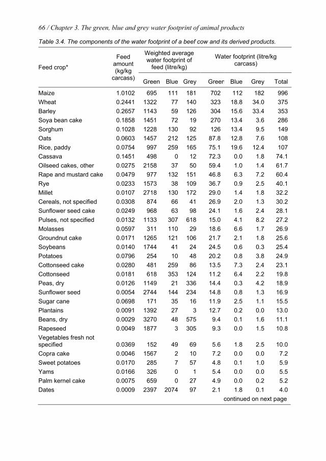
66 / Chapter 3. The green, blue and grey water footprint of animal products
Table 3.4. The components of the water footprint of a beef cow and its derived products.
Feed crop*
Feed amount (kg/kg
carcass)
Weighted average water footprint of
feed (litre/kg)
Water footprint (litre/kg carcass)
Green Blue Grey Green Blue Grey Total
Maize 1.0102 695 111 181 702 112 182 996 Wheat 0.2441 1322 77 140 323 18.8 34.0 375 Barley 0.2657 1143 59 126 304 15.6 33.4 353 Soya bean cake 0.1858 1451 72 19 270 13.4 3.6 286 Sorghum 0.1028 1228 130 92 126 13.4 9.5 149 Oats 0.0603 1457 212 125 87.8 12.8 7.6 108 Rice, paddy 0.0754 997 259 165 75.1 19.6 12.4 107 Cassava 0.1451 498 0 12 72.3 0.0 1.8 74.1 Oilseed cakes, other 0.0275 2158 37 50 59.4 1.0 1.4 61.7 Rape and mustard cake 0.0479 977 132 151 46.8 6.3 7.2 60.4 Rye 0.0233 1573 38 109 36.7 0.9 2.5 40.1 Millet 0.0107 2718 130 172 29.0 1.4 1.8 32.2 Cereals, not specified 0.0308 874 66 41 26.9 2.0 1.3 30.2 Sunflower seed cake 0.0249 968 63 98 24.1 1.6 2.4 28.1 Pulses, not specified 0.0132 1133 307 618 15.0 4.1 8.2 27.2 Molasses 0.0597 311 110 29 18.6 6.6 1.7 26.9 Groundnut cake 0.0171 1265 121 106 21.7 2.1 1.8 25.6 Soybeans 0.0140 1744 41 24 24.5 0.6 0.3 25.4 Potatoes 0.0796 254 10 48 20.2 0.8 3.8 24.9 Cottonseed cake 0.0280 481 259 86 13.5 7.3 2.4 23.1 Cottonseed 0.0181 618 353 124 11.2 6.4 2.2 19.8 Peas, dry 0.0126 1149 21 336 14.4 0.3 4.2 18.9 Sunflower seed 0.0054 2744 144 234 14.8 0.8 1.3 16.9 Sugar cane 0.0698 171 35 16 11.9 2.5 1.1 15.5 Plantains 0.0091 1392 27 3 12.7 0.2 0.0 13.0 Beans, dry 0.0029 3270 48 575 9.4 0.1 1.6 11.1 Rapeseed 0.0049 1877 3 305 9.3 0.0 1.5 10.8 Vegetables fresh not specified 0.0369 152 49 69 5.6 1.8 2.5 10.0 Copra cake 0.0046 1567 2 10 7.2 0.0 0.0 7.2 Sweet potatoes 0.0170 285 7 57 4.8 0.1 1.0 5.9 Yams 0.0166 326 0 1 5.4 0.0 0.0 5.5 Palm kernel cake 0.0075 659 0 27 4.9 0.0 0.2 5.2 Dates 0.0009 2397 2074 97 2.1 1.8 0.1 4.0
continued on next page
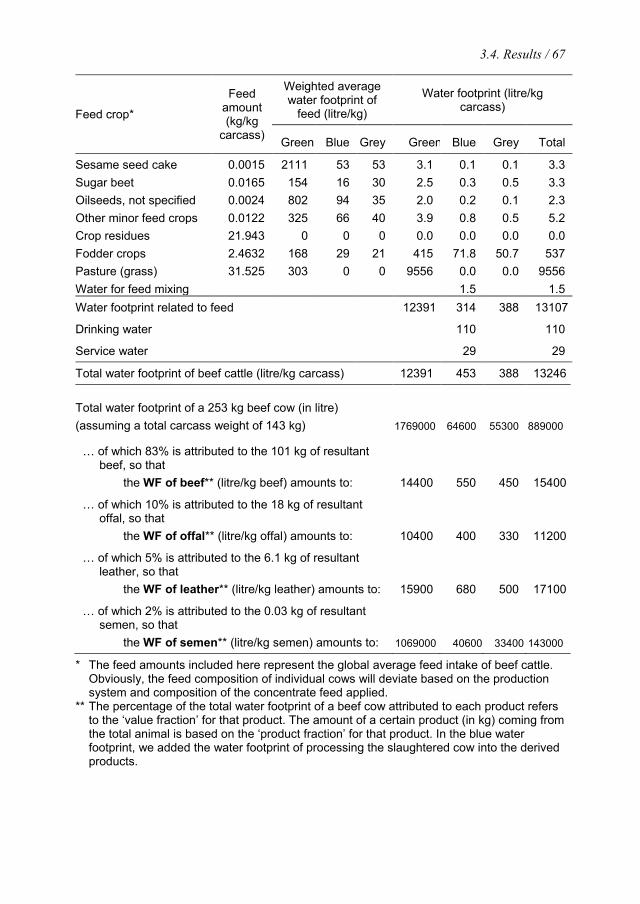
3.4. Results / 67
Feed crop*
Feed amount (kg/kg
carcass)
Weighted average water footprint of
feed (litre/kg)
Water footprint (litre/kg carcass)
Green Blue Grey Green Blue Grey Total
Sesame seed cake 0.0015 2111 53 53 3.1 0.1 0.1 3.3 Sugar beet 0.0165 154 16 30 2.5 0.3 0.5 3.3 Oilseeds, not specified 0.0024 802 94 35 2.0 0.2 0.1 2.3 Other minor feed crops 0.0122 325 66 40 3.9 0.8 0.5 5.2 Crop residues 21.943 0 0 0 0.0 0.0 0.0 0.0 Fodder crops 2.4632 168 29 21 415 71.8 50.7 537 Pasture (grass) 31.525 303 0 0 9556 0.0 0.0 9556 Water for feed mixing 1.5 1.5 Water footprint related to feed 12391 314 388 13107
Drinking water 110 110
Service water 29 29
Total water footprint of beef cattle (litre/kg carcass) 12391 453 388 13246
Total water footprint of a 253 kg beef cow (in litre) (assuming a total carcass weight of 143 kg) 1769000 64600 55300 889000
… of which 83% is attributed to the 101 kg of resultant beef, so that
the WF of beef** (litre/kg beef) amounts to: 14400 550 450 15400
… of which 10% is attributed to the 18 kg of resultant offal, so that
the WF of offal** (litre/kg offal) amounts to: 10400 400 330 11200
… of which 5% is attributed to the 6.1 kg of resultant leather, so that
the WF of leather** (litre/kg leather) amounts to: 15900 680 500 17100
… of which 2% is attributed to the 0.03 kg of resultant semen, so that
the WF of semen** (litre/kg semen) amounts to: 1069000 40600 33400 143000
* The feed amounts included here represent the global average feed intake of beef cattle. Obviously, the feed composition of individual cows will deviate based on the production system and composition of the concentrate feed applied.
** The percentage of the total water footprint of a beef cow attributed to each product refers to the ‘value fraction’ for that product. The amount of a certain product (in kg) coming from the total animal is based on the ‘product fraction’ for that product. In the blue water footprint, we added the water footprint of processing the slaughtered cow into the derived products.
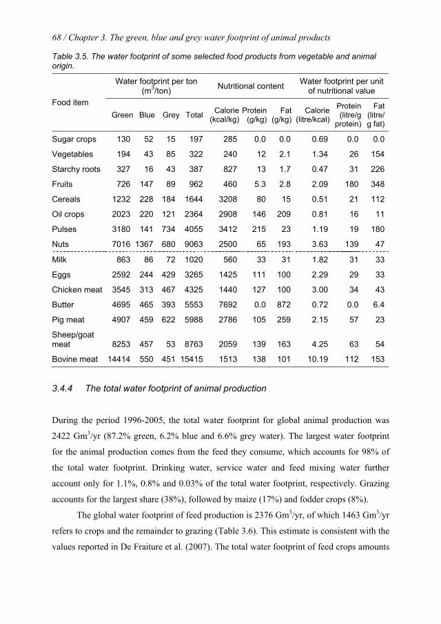
68 / Chapter 3. The green, blue and grey water footprint of animal products
Table 3.5. The water footprint of some selected food products from vegetable and animal origin.
Food item
Water footprint per ton (m3/ton) Nutritional content Water footprint per unit
of nutritional value
Green Blue Grey Total Calorie (kcal/kg)
Protein (g/kg)
Fat (g/kg)
Calorie (litre/kcal)
Protein (litre/g
protein)
Fat (litre/g fat)
Sugar crops 130 52 15 197 285 0.0 0.0 0.69 0.0 0.0
Vegetables 194 43 85 322 240 12 2.1 1.34 26 154
Starchy roots 327 16 43 387 827 13 1.7 0.47 31 226
Fruits 726 147 89 962 460 5.3 2.8 2.09 180 348
Cereals 1232 228 184 1644 3208 80 15 0.51 21 112
Oil crops 2023 220 121 2364 2908 146 209 0.81 16 11
Pulses 3180 141 734 4055 3412 215 23 1.19 19 180
Nuts 7016 1367 680 9063 2500 65 193 3.63 139 47
Milk 863 86 72 1020 560 33 31 1.82 31 33
Eggs 2592 244 429 3265 1425 111 100 2.29 29 33
Chicken meat 3545 313 467 4325 1440 127 100 3.00 34 43
Butter 4695 465 393 5553 7692 0.0 872 0.72 0.0 6.4
Pig meat 4907 459 622 5988 2786 105 259 2.15 57 23
Sheep/goat meat 8253 457 53 8763 2059 139 163 4.25 63 54
Bovine meat 14414 550 451 15415 1513 138 101 10.19 112 153
3.4.4 The total water footprint of animal production
During the period 1996-2005, the total water footprint for global animal production was
2422 Gm3/yr (87.2% green, 6.2% blue and 6.6% grey water). The largest water footprint
for the animal production comes from the feed they consume, which accounts for 98% of
the total water footprint. Drinking water, service water and feed mixing water further
account only for 1.1%, 0.8% and 0.03% of the total water footprint, respectively. Grazing
accounts for the largest share (38%), followed by maize (17%) and fodder crops (8%).
The global water footprint of feed production is 2376 Gm3/yr, of which 1463 Gm3/yr
refers to crops and the remainder to grazing (Table 3.6). This estimate is consistent with the
values reported in De Fraiture et al. (2007). The total water footprint of feed crops amounts
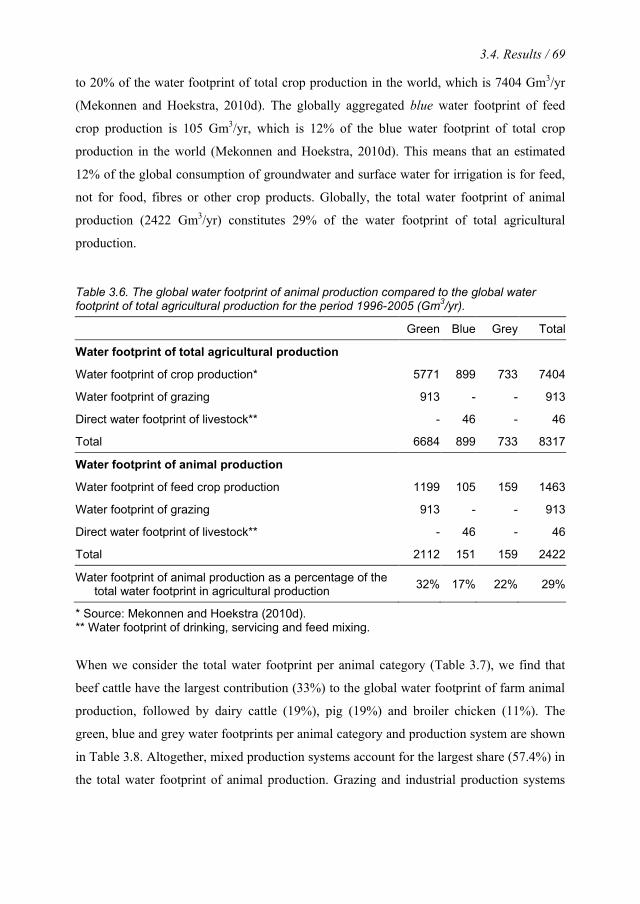
3.4. Results / 69
to 20% of the water footprint of total crop production in the world, which is 7404 Gm3/yr
(Mekonnen and Hoekstra, 2010d). The globally aggregated blue water footprint of feed
crop production is 105 Gm3/yr, which is 12% of the blue water footprint of total crop
production in the world (Mekonnen and Hoekstra, 2010d). This means that an estimated
12% of the global consumption of groundwater and surface water for irrigation is for feed,
not for food, fibres or other crop products. Globally, the total water footprint of animal
production (2422 Gm3/yr) constitutes 29% of the water footprint of total agricultural
production.
Table 3.6. The global water footprint of animal production compared to the global water footprint of total agricultural production for the period 1996-2005 (Gm3/yr).
Green Blue Grey Total
Water footprint of total agricultural production
Water footprint of crop production* 5771 899 733 7404
Water footprint of grazing 913 - - 913
Direct water footprint of livestock** - 46 - 46
Total 6684 899 733 8317
Water footprint of animal production
Water footprint of feed crop production 1199 105 159 1463
Water footprint of grazing 913 - - 913
Direct water footprint of livestock** - 46 - 46
Total 2112 151 159 2422
Water footprint of animal production as a percentage of the total water footprint in agricultural production 32% 17% 22% 29%
* Source: Mekonnen and Hoekstra (2010d). ** Water footprint of drinking, servicing and feed mixing.
When we consider the total water footprint per animal category (Table 3.7), we find that
beef cattle have the largest contribution (33%) to the global water footprint of farm animal
production, followed by dairy cattle (19%), pig (19%) and broiler chicken (11%). The
green, blue and grey water footprints per animal category and production system are shown
in Table 3.8. Altogether, mixed production systems account for the largest share (57.4%) in
the total water footprint of animal production. Grazing and industrial production systems

70 / Chapter 3. The green, blue and grey water footprint of animal products
account for 20.3% and 22.3%, respectively. In the grazing system, over 97% of the water
footprint related to feed comes from grazing and fodder crops and the water footprint is
dominantly (94%) green. In the mixed and industrial production systems, the green water
footprint forms 87% and 82% of the total footprint, respectively. The blue water footprint
in the grazing system accounts for 3.6% of the total water footprint and about 33% of this
comes from the drinking and service water use. In the industrial system, the blue water
footprint accounts for 8% of the total water footprint.
A substantial part of the water footprint of an animal product produced in one
country often resides outside that country. This is most in particular the case for products
originating from industrial production systems, because those systems use the largest
fraction of concentrate feed. Feed crops are often imported rather than produced
domestically. Soybean cake, for example, which is an important feed ingredient in
industrial livestock raising, is often imported. In the period 1996-2005, 49% of global
soybean production was exported, either in the form of soybean or in the form of soybean
cake (FAO, 2010a).
Table 3.7. The total water footprint per animal category (1996-2005).
Animal category
Global total number of
animals* (millions)
Average annual water footprint per animal**
(m3/yr per animal)
Annual water footprint of animal category (Gm3/yr)
%
Beef cattle 1267 630 798 33
Dairy cattle 228 2056 469 19
Pig 880 520 458 19
Broiler chicken 9923 26 255 11
Horse 112 1599 180 7
Layer Chicken 5046 33 167 7
Sheep 1052 68 71 3
Goat 750 32 24 1
Total 19258 2422 100
* Source: FAO (2010a). ** See Table 3.2.
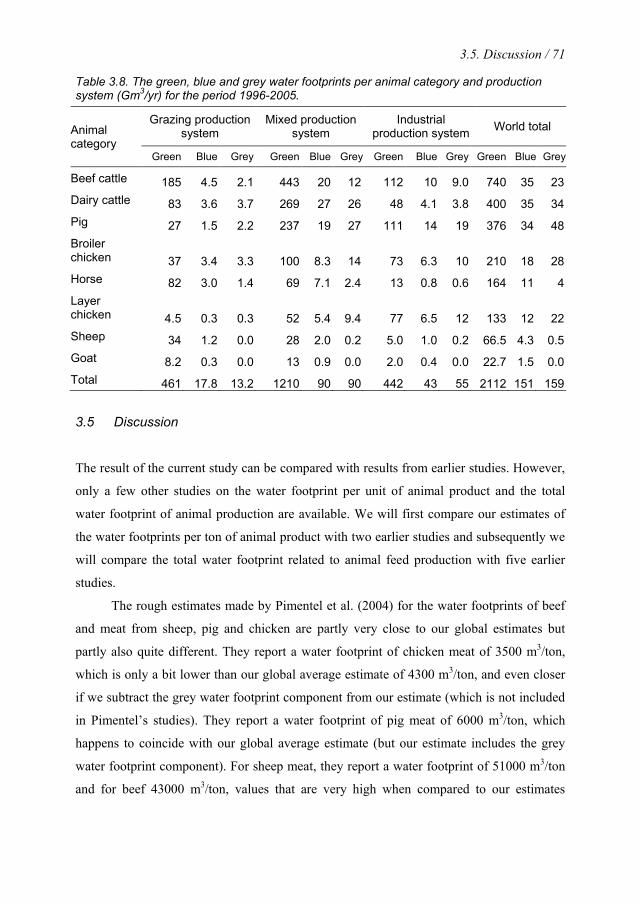
3.5. Discussion / 71
Table 3.8. The green, blue and grey water footprints per animal category and production system (Gm3/yr) for the period 1996-2005.
Animal category
Grazing production system
Mixed production system
Industrial production system World total
Green Blue Grey Green Blue Grey Green Blue Grey Green Blue Grey
Beef cattle 185 4.5 2.1 443 20 12 112 10 9.0 740 35 23 Dairy cattle 83 3.6 3.7 269 27 26 48 4.1 3.8 400 35 34 Pig 27 1.5 2.2 237 19 27 111 14 19 376 34 48 Broiler chicken 37 3.4 3.3 100 8.3 14 73 6.3 10 210 18 28 Horse 82 3.0 1.4 69 7.1 2.4 13 0.8 0.6 164 11 4 Layer chicken 4.5 0.3 0.3 52 5.4 9.4 77 6.5 12 133 12 22 Sheep 34 1.2 0.0 28 2.0 0.2 5.0 1.0 0.2 66.5 4.3 0.5 Goat 8.2 0.3 0.0 13 0.9 0.0 2.0 0.4 0.0 22.7 1.5 0.0 Total 461 17.8 13.2 1210 90 90 442 43 55 2112 151 159
3.5 Discussion
The result of the current study can be compared with results from earlier studies. However,
only a few other studies on the water footprint per unit of animal product and the total
water footprint of animal production are available. We will first compare our estimates of
the water footprints per ton of animal product with two earlier studies and subsequently we
will compare the total water footprint related to animal feed production with five earlier
studies.
The rough estimates made by Pimentel et al. (2004) for the water footprints of beef
and meat from sheep, pig and chicken are partly very close to our global estimates but
partly also quite different. They report a water footprint of chicken meat of 3500 m3/ton,
which is only a bit lower than our global average estimate of 4300 m3/ton, and even closer
if we subtract the grey water footprint component from our estimate (which is not included
in Pimentel’s studies). They report a water footprint of pig meat of 6000 m3/ton, which
happens to coincide with our global average estimate (but our estimate includes the grey
water footprint component). For sheep meat, they report a water footprint of 51000 m3/ton
and for beef 43000 m3/ton, values that are very high when compared to our estimates
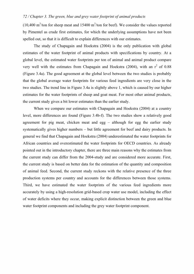
72 / Chapter 3. The green, blue and grey water footprint of animal products
(10,400 m3/ton for sheep meat and 15400 m3/ton for beef). We consider the values reported
by Pimentel as crude first estimates, for which the underlying assumptions have not been
spelled out, so that it is difficult to explain differences with our estimates.
The study of Chapagain and Hoekstra (2004) is the only publication with global
estimates of the water footprint of animal products with specifications by country. At a
global level, the estimated water footprints per ton of animal and animal product compare
very well with the estimates from Chapagain and Hoekstra (2004), with an r2 of 0.88
(Figure 3.4a). The good agreement at the global level between the two studies is probably
that the global average water footprints for various feed ingredients are very close in the
two studies. The trend line in Figure 3.4a is slightly above 1, which is caused by our higher
estimates for the water footprints of sheep and goat meat. For most other animal products,
the current study gives a bit lower estimates than the earlier study.
When we compare our estimates with Chapagain and Hoekstra (2004) at a country
level, more differences are found (Figure 3.4b-f). The two studies show a relatively good
agreement for pig meat, chicken meat and egg – although for egg the earlier study
systematically gives higher numbers – but little agreement for beef and dairy products. In
general we find that Chapagain and Hoekstra (2004) underestimated the water footprints for
African countries and overestimated the water footprints for OECD countries. As already
pointed out in the introductory chapter, there are three main reasons why the estimates from
the current study can differ from the 2004-study and are considered more accurate. First,
the current study is based on better data for the estimation of the quantity and composition
of animal feed. Second, the current study reckons with the relative presence of the three
production systems per country and accounts for the differences between those systems.
Third, we have estimated the water footprints of the various feed ingredients more
accurately by using a high-resolution grid-based crop water use model, including the effect
of water deficits where they occur, making explicit distinction between the green and blue
water footprint components and including the grey water footprint component.
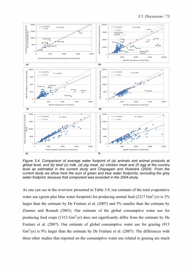
3.5. Discussion / 73
R² = 0.6972
0
5000
10000
15000
20000
0 5000 10000 15000 20000
Egg
WF
estim
ate
from
curre
nt st
udy
[m3 /t
on]
Egg WF estimate from ref. 26 [m3/ton]
trend line
1:1 lineR² = 0.8717
0
5000
10000
15000
20000
0 5000 10000 15000 20000
Chi
cken
mea
t WF
estim
ate
from
curre
nt st
udy
[m3 /t
on]
Chicken meat WF estimate from ref. 26 [m3/ton]
trend line
1:1 line
R² = 0.2649
0
25000
50000
75000
100000
0 25000 50000 75000 100000
Beef
WF
estim
ate
from
curre
nt st
udy
[m3 /t
on]
Beef WF estimate from ref. 26 [m3/ton]
trend line
1:1 line
Tunisia
Syria
Ertrea
Mexico
Cyprus
Mongolia
Bolivia
Spain
Benin
Morocco
Mostly African countries
Mostly OECD countries
(a) (b)
(c) (d)
(e) (f)
milk
goat meat
pig meat
sheep meat
beef cattle
beef
R² = 0.8773
0
5000
10000
15000
20000
0 5000 10000 15000 20000
Anim
als a
nd a
nim
al p
rodu
cts W
F es
timat
e fro
m cu
rrent
stud
y [m
3 /ton
]
Animals and animal products WF estimate from ref. 26 [m3/ton]
trend line1:1 line
R² = 0.4798
0
2500
5000
7500
10000
0 2500 5000 7500 10000
Milk
WF
estim
ate
from
curre
nt st
udy
[m3 /t
on]
Milk WF estimate from ref. 26 [m3/ton]
trend line
1:1 line
Mongolia
HungaryGeorgia
SenegalMauritania
Niger
R² = 0.7929
0
5000
10000
15000
20000
0 5000 10000 15000 20000Po
rtk W
F es
timat
e fro
m cu
rrent
stud
y [m
3 /ton
]
Pork WF estimate from ref. 26 [m3/ton]
trend line
1:1 line
Tajikstan
Figure 3.4. Comparison of average water footprint of (a) animals and animal products at global level, and (b) beef (c) milk, (d) pig meat, (e) chicken meat and (f) egg at the country level as estimated in the current study and Chapagain and Hoekstra (2004). From the current study we show here the sum of green and blue water footprints, excluding the grey water footprint, because that component was excluded in the 2004-study.
As one can see in the overview presented in Table 3.9, our estimate of the total evaporative
water use (green plus blue water footprint) for producing animal feed (2217 Gm3/yr) is 3%
larger than the estimate by De Fraiture et al. (2007) and 5% smaller than the estimate by
Zimmer and Renault (2003). Our estimate of the global consumptive water use for
producing feed crops (1312 Gm3/yr) does not significantly differ from the estimate by De
Fraiture et al. (2007). Our estimate of global consumptive water use for grazing (913
Gm3/yr) is 9% larger than the estimate by De Fraiture et al. (2007). The differences with
three other studies that reported on the consumptive water use related to grazing are much
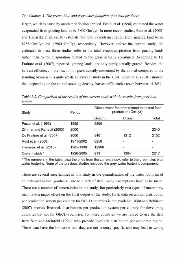
74 / Chapter 3. The green, blue and grey water footprint of animal products
larger, which is cause by another definition applied. Postel et al. (1996) estimated the water
evaporated from grazing land to be 5800 Gm3/yr. In more recent studies, Rost et al. (2008)
and Hanasaki et al. (2010) estimate the total evapotranspiration from grazing land to be
8258 Gm3/yr and 12960 Gm3/yr, respectively. However, unlike the current study, the
estimates in these three studies refer to the total evapotranspiration from grazing lands
rather than to the evaporation related to the grass actually consumed. According to De
Fraiture et al. (2007), reported ‘grazing lands’ are only partly actually grazed. Besides, the
harvest efficiency – the fraction of grass actually consumed by the animal compared to the
standing biomass – is quite small. In a recent study in the USA, Smart et al. (2010) showed
that, depending on the animal stocking density, harvest efficiencies reach between 14-38%.
Table 3.9. Comparison of the results of the current study with the results from previous studies.
Study Period Global water footprint related to animal feed
production (Gm3/yr)*
Grazing Crops Total Postel et al. (1996) 1995 5800 - -
Zimmer and Renault (2003) 2000 - - 2340
De Fraiture et al. (2007) 2000 840 1312 2152
Rost et al. (2008) 1971-2002 8258 - -
Hanasaki et al. (2010) 1985-1999 12960 - -
Current study* 1996-2005 913 1304 2217
* The numbers in the table, also the ones from the current study, refer to the green plus blue water footprint. None of the previous studies included the grey water footprint component.
There are several uncertainties in this study in the quantification of the water footprint of
animals and animal products. Due to a lack of data, many assumptions have to be made.
There are a number of uncertainties in the study, but particularly two types of uncertainty
may have a major effect on the final output of the study. First, data on animal distribution
per production system per country for OECD countries is not available. Wint and Robinson
(2007) provide livestock distributions per production system per country for developing
countries but not for OECD countries. For these countries we are forced to use the data
from Seré and Steinfeld (1996), who provide livestock distribution per economic region.
These data have the limitation that they are not country-specific and may lead to wrong
3.6. Conclusion / 75
distribution of animals into the different production system for some countries. The second
major uncertainty is related to the precise composition of feed per animal category per
country. Such data are not directly available so that we had to infer these data by combining
different data sources and a number of assumptions.
Although the scope of this study is very comprehensive, there are many issues that
have been left out. One issue is that we neglected the indirect water footprints of materials
used in feed production and animal raising. We expect that this may add at most a few per
cents to the water footprint estimates found in this study (based on Hoekstra et al., 2009). In
the grey water footprint estimations we have looked at the water pollution by nitrogen-
fertilisers only, excluding the potential pollution by other fertiliser components or by
pesticides or other agro-chemicals. Besides, we have not quantified the grey water footprint
coming from animal wastes, which is particularly relevant for industrial production
systems. Intensive animal production often generates an amount of waste that cannot be
fully recycled on the nearby land. The large amount of waste generated in a concentrated
place can seriously affect freshwater systems (FAO, 2005b; Steinfeld et al., 2006;
Galloway et al., 2007). Finally, by focusing on freshwater appropriation, the study
obviously excludes many other relevant issues in farm animal production, such as micro-
and macro-cost of production, livelihood of smallholder farmers, animal welfare, public
health and environmental issues other than freshwater.
3.6 Conclusion
The present study estimates the water footprint of farm animals and animal products per
production system and per country. The results show that:
• The blue and grey water footprints of animal products are largest for industrial systems
(with an exception for chicken products). From a freshwater perspective, animal
products from grazing systems are therefore to be preferred above products from
industrial systems.
• The water footprint of any animal product is larger than the water footprint of a wisely
chosen crop product with equivalent nutritional value.

76 / Chapter 3. The green, blue and grey water footprint of animal products
• 29% of the total water footprint of the agricultural sector in the world is related to the
production of animal products. One third of the global water footprint of animal
production is related to beef cattle.
Managing the demand for animal products by promoting a dietary shift away from a meat-
rich diet will be an inevitable component in the environmental policy of governments. In
countries where the consumption of animal products is still quickly rising, one should
critically look how this growing demand can be moderated. On the production side, it
would be wise to include freshwater implications in the development of animal farming
policies, which means that particularly feed composition, feed water requirements and feed
origin need to receive attention. Animal farming puts the lowest pressure on freshwater
systems when dominantly based on crop residues, waste and roughages. Policies aimed to
influence either the consumption or production side of farm animal products will generally
entail various sorts of socio-economic and environmental trade-offs (Herrero et al., 2009;
Pelletier and Tyedmers, 2010). Therefore, policies aimed at reducing the negative impacts
of animal production and consumption should be able to address these potential tradeoffs.
Policies should not affect the required increase in food security in less developed countries
neither the livelihood of the rural poor should be put in danger through intensification of
animal farming.
This study provides a rich data source for further studies on the factors that
determine how animal products put pressure on the global water resources. The reported
incidents of groundwater depletion, rivers running dry and increasing levels of pollution
form an indication of the growing water scarcity (UNESCO, 2009; Postel, 2000; Gleick,
1993). Since animal production and consumption play an important role in depleting and
polluting the world’s scarce freshwater resources, information on the water footprint of
animal products will help us understand how we can sustain the scarce freshwater
resources.
4. National water footprint accounts: the green, blue and grey water footprint of production and consumption3
Abstract
This study quantifies and maps the water footprints of nations from both a production and
consumption perspective and estimates international virtual water flows and national and
global water savings as a result of trade. The entire estimate includes a breakdown of water
footprints, virtual water flows and water savings into their green, blue and grey
components. The main finding of the study can be summarized as:
• The global water footprint in the period 1996-2005 was 9087 Gm3/yr (74% green, 11%
blue, 15% grey). Agricultural production contributes 92% to this total footprint.
• About one fifth of the global water footprint relates to production for export.
• The total volume of international virtual water flows related to trade in agricultural and
industrial products was 2320 Gm3/yr (68% green, 13% blue, 19% grey). Trade in crop
products contributes 76% to the total volume of international virtual water flows; trade
in animal and industrial products contribute 12% each. As a global average, the blue
and grey shares in the total water footprint of internationally traded products are
slightly larger than in the case of domestically consumed products.
• Mexico and Spain are the two countries with the largest national blue water savings as
a result of trade.
• The global water saving as a result of trade in agricultural products in the period 1996-
2005 was 369 Gm3/yr (59% green, 27% blue, 15% grey), which is equivalent to 4% of
the global water footprint related to agricultural production. The global blue water
saving is equivalent to 10% of the global blue water footprint related to agricultural
production, which indicates that virtual water importing countries generally depend
more strongly on blue water for crop production than the virtual water exporting
countries. The largest global water saving (53%) is due to trade in cereal crops,
followed by oil crops (22%) and animal products (15%).
3 Based on Mekonnen and Hoekstra (2011b)
78 / Chapter 4. National water footprint accounts
• International trade in industrial products can be associated with an increased global
water footprint that is equivalent to 4% of the global water footprint related to
industrial production.
• The water footprint of the global average consumer in the period 1996-2005 was 1385
m3/yr. About 92% of the water footprint is related to the consumption of agricultural
products, 5% to the consumption of industrial goods, and 4% to domestic water use.
• The average consumer in the US has a water footprint of 2842 m3/yr, while the average
citizens in China and India have water footprints of 1071 m3/yr and 1089 m3/yr
respectively.
• Consumption of cereal products gives the largest contribution to the water footprint of
the average consumer (27%), followed by meat (22%) and milk products (7%). The
contribution of different consumption categories to the total water footprint varies
across countries.
• The volume and pattern of consumption and the water footprint per ton of product of
the products consumed are the main factors determining the water footprint of a
consumer.
The study illustrates the global dimension of water consumption and pollution by showing
that several countries heavily rely on water resources elsewhere (for example Mexico
depending on virtual water imports from the US) and that many countries have significant
impacts on water consumption and pollution elsewhere (for example Japan and many
European countries due to their large external water footprints).
4.1 Introduction
The earth’s freshwater resources are subject to increasing pressure in the form of
consumptive water use and pollution (Postel, 2000; WWAP, 2003, 2006, 2009). Until
recently, issues of freshwater availability, use and management have been addressed at a
local, national and river basin scale. The recognition that freshwater resources are subject to
global changes and globalization have led a number of researchers to argue for the
importance of putting freshwater issues in a global context (Postel et al., 1996; Vörösmarty
et al., 2000; Hoekstra and Hung, 2005; Hoekstra and Chapagain, 2008; Hoff, 2009).

4.1. Introduction / 79
Appreciating the global dimension of freshwater resources can be regarded as a key to
solving some of today’s most urgent water problems (Hoekstra, 2011).
In formulating national water plans, governments have traditionally taken a purely
national perspective, aiming at matching national water supplies to national water demands.
Governments have looked for ways to satisfy water users without questioning the total
amount of water demands. Even though governments nowadays consider options to reduce
water demands, in addition to options to increase supplies, they generally do not consider
the global dimension of water demand patterns. All countries trade water-intensive
commodities, but few governments explicitly consider options to save water through import
of water-intensive products or to make use of relative water abundance to produce water-
intensive commodities for export. In addition, by looking at water use within only their own
country, governments do not have a comprehensive view of the sustainability of national
consumption. Many countries have significantly externalized their water footprint without
looking at whether the imported products are related to water depletion or pollution in the
producing countries. Knowledge of the dependency on water resources elsewhere is
relevant for a national government, not only when evaluating its environmental policy but
also when assessing national food security.
Understanding the water footprint of a nation is highly relevant for developing well-
informed national policy. Conventional national water use accounts are restricted to
statistics on water withdrawals within their own territory (Van der Leeden et al., 1990;
Gleick, 1993; FAO, 2010b). National water footprint accounts extend these statistics by
including data on green water use and volumes of water use for waste assimilation and by
adding data on water use in other countries for producing imported products as well as data
on water use within the country for making export products (Hoekstra et al., 2011).
Quantifying and mapping ‘national water footprints’ is an evolving field of study
since the introduction of the water footprint concept in the beginning of this century
(Hoekstra, 2003). The first global study on the water footprints of nations was carried out
by Hoekstra and Hung (2002); a second, much more comprehensive study, was done by
Hoekstra and Chapagain and reported in a number of subsequent publications: Chapagain
and Hoekstra (2004, 2008), Chapagain et al. (2006a) and Hoekstra and Chapagain (2007a,
2008). The current study is the third global assessment of national water footprints, which
80 / Chapter 4. National water footprint accounts
improves upon the previous assessments in a number of respects as will be elaborated
below.
The objective of this study is to estimate the water footprints of nations from both a
production and consumption perspective. First, the green, blue and grey water footprints
within countries associated with agricultural production, industrial production and domestic
water supply is quantified and mapped at a high spatial resolution. Second, international
virtual water flows related to trade in agricultural and industrial commodities is estimated.
Finally, the water footprint of consumption for all countries of the world distinguishing for
each country between the internal and the external water footprint of national consumption
is quantified and mapped. Throughout the study, the green, blue and grey water footprints
are explicitly distinguished.
The current study is more comprehensive and detailed than the earlier two global
water footprint studies (Hoekstra and Hung, 2002; Hoekstra and Chapagain, 2008). It is
also more comprehensive than the contemporary study by Fader et al. (2011), who estimate
the global green and blue water footprint of consumption showing the internal and external
water footprint per country. This study excludes the grey water footprint component and is
restricted to an analysis of the water footprint of consuming crop products, leaving out the
water footprints of farm animal products, industrial products and domestic water supply.
Apart from the global water footprint studies mentioned, several water footprint
studies with a focus on a specific country were published in the past few years: Vincent et
al. (2011) for Belgium; Ma et al. (2006), Liu and Savenije (2008), Hubacek et al. (2009)
and Zhao et al. (2009) for China; Sonnenberg et al. (2009) for Germany; Kampman et al.
(2008) for India; Bulsink et al. (2009) for Indonesia; Hoekstra and Chapagain (2007b) for
Morocco; Hoekstra and Chapagain (2007b) and Van Oel et al. (2009) for the Netherlands;
Aldaya et al. (2010a) and Garrido et al. (2010) for Spain; Sonnenberg et al. (2010) for
Switzerland; Chahed et al. (2008) for Tunisia; and Chapagain and Orr (2008), Yu et al.
(2010) and Feng et al. (2011) for the UK. The scope, assumptions and data sources in these
country studies vary widely, so these studies cannot be used to make comparisons between
countries.
The study improves upon the previous global water footprint study – Hoekstra and
Chapagain (2008) – in a number of respects: applied a high spatial resolution in estimating
the water footprint in crop production, industrial production and domestic water supply. In
4.2. Method and data / 81
the case of crop production, made an explicit distinction between the green, blue and grey
water footprint; used better estimates of the feed composition of farm animals and
distinguished three different animal production systems (grazing, mixed and industrial) in
each country, accounting for the relative presence of those three systems; explicitly
distinguished between the blue and grey water footprint in industrial production and
domestic water supply and account for wastewater treatment coverage per country; applied
the bottom-up approach in estimating the water footprint of national consumption of
agricultural products, which is less sensitive to trade data than the top-down approach.
The study builds on two earlier studies by the same authors. In Mekonnen and
Hoekstra (2010d, 2011a) we have reported the green, blue and grey water footprints of
crops and derived crop products. In Mekonnen and Hoekstra (2010e) we documented the
green, blue and grey water footprints of farm animals and animal products.
4.2 Method and data
Accounting framework
In this study we adopt the terminology and calculation methodology as set out in The Water
Footprint Assessment Manual, which contains the global standard for water footprint
assessment developed by the Water Footprint Network (Hoekstra et al., 2011). The ‘water
footprint’ is a measure of human’s appropriation of freshwater resources. Freshwater
appropriation is measured in terms of water volumes consumed (evaporated or incorporated
into a product) or polluted per unit of time. A water footprint has three components: green,
blue and grey. The blue water footprint refers to consumption of blue water resources
(surface and ground water). The green water footprint is the volume of green water
(rainwater) consumed, which is particularly relevant in crop production. The grey water
footprint is an indicator of the degree of freshwater pollution and is defined as the volume
of freshwater that is required to assimilate the load of pollutants based on existing ambient
water quality standards. The water footprint is a geographically explicit indicator, showing
not only volumes of water consumption and pollution, but also the locations.
The framework for national water footprint accounting is shown in Figure 4.1. One
can see that ‘the water footprint of national consumption’ is different from ‘the water
footprint within the area of the nation’. The latter is the water footprint of national
82 / Chapter 4. National water footprint accounts
production, defined as the total freshwater volume consumed or polluted within the
territory of the nation as a result of activities within the different sectors of the economy. It
can be calculated by summing the water footprints of all water consuming or polluting
processes taking place in the nation. Generally, one can distinguish three main water using
sectors: the agricultural sector, the industrial sector and the domestic water supply sector.
On the other hand, the water footprint of national consumption is defined as the total
volume of freshwater that is used to produce the goods and services consumed by the
inhabitant of the nation. It consists of two components: the internal and external water
footprint of national consumption. The internal water footprint is defined as the use of
domestic water resources to produce goods and services consumed by the nation’s
population. It is the sum of the water footprint within the nation minus the volume of
virtual-water export to other nations related to the export of products produced with
domestic water resources. The external water footprint is defined as the volume of water
resources used in other nations to produce goods and services consumed by the population
in the nation under consideration. It is equal to the virtual-water import into the nation
minus the volume of virtual-water export to other nations as a result of re-export of
imported products. The virtual-water export from a nation consists of exported water of
domestic origin and re-exported water of foreign origin. The virtual-water import into a
nation will partly be consumed, thus constituting the external water footprint of national
consumption, and may partly be re-exported. The sum of the virtual water import into a
country and the water footprint within the area of the nation is equal to the sum of the
virtual water export from the nation and the water footprint of national consumption. This
sum is called the virtual-water budget of a nation.
Water footprints of national production
The water footprints within nations related to crop production were obtained from
Mekonnen and Hoekstra (2010b, 2010d, 2011a), who estimated the global water footprint
of crop production with a crop water use model at a 5 by 5 arc minute spatial resolution.
The water footprints within nations related to water use in livestock farming, were obtained
from Mekonnen and Hoekstra (2010e). The water footprints within nations related to
industrial production and domestic water supply were estimated in this study using water
withdrawal data from the AQUASTAT database (FAO, 2010b). For some countries, water
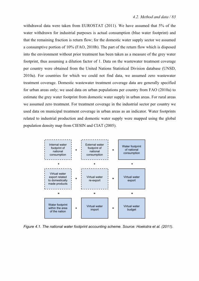
4.2. Method and data / 83
withdrawal data were taken from EUROSTAT (2011). We have assumed that 5% of the
water withdrawn for industrial purposes is actual consumption (blue water footprint) and
that the remaining fraction is return flow; for the domestic water supply sector we assumed
a consumptive portion of 10% (FAO, 2010b). The part of the return flow which is disposed
into the environment without prior treatment has been taken as a measure of the grey water
footprint, thus assuming a dilution factor of 1. Data on the wastewater treatment coverage
per country were obtained from the United Nations Statistical Division database (UNSD,
2010a). For countries for which we could not find data, we assumed zero wastewater
treatment coverage. Domestic wastewater treatment coverage data are generally specified
for urban areas only; we used data on urban populations per country from FAO (2010a) to
estimate the grey water footprint from domestic water supply in urban areas. For rural areas
we assumed zero treatment. For treatment coverage in the industrial sector per country we
used data on municipal treatment coverage in urban areas as an indicator. Water footprints
related to industrial production and domestic water supply were mapped using the global
population density map from CIESIN and CIAT (2005).
Figure 4.1. The national water footprint accounting scheme. Source: Hoekstra et al. (2011).
Internal water footprint of
national consumption
External water footprint of
national consumption
+ Water footprint
of national consumption
=
Virtual water export related to domestically made products
Virtual water re-export + Virtual water
export =
+ + +
Water footprint within the area of the nation
Virtual water import + Virtual water
budget =
= = =

84 / Chapter 4. National water footprint accounts
International virtual water flows
International virtual-water flows are calculated by multiplying, per trade commodity, the
volume of trade by the respective average water footprint per ton of product in the
exporting nation. When a product is exported from a country that does not produce the
product we have assumed the global average product water footprint for that trade flow.
Data on international trade in agricultural and industrial products have been taken from the
SITA database (Statistics for International Trade Analysis) available from the International
Trade Centre (ITC, 2007). This database covers trade data over ten years (1996-2005) from
230 reporting countries disaggregated by product and partner countries. Country-specific
estimates on the green, blue and grey water footprints of 146 crops and more than two
hundred derived crop products per ton of product were taken from Mekonnen and Hoekstra
(2010d). Estimates on the water footprints of farm animals (beef cattle, dairy cattle, pig,
sheep, goat, broiler chicken, layer chicken and horses) and animal products per ton of
product were taken from Mekonnen and Hoekstra (2010e). The national average water
footprint per dollar of industrial product was calculated per country by dividing the total
national water footprint in the industrial sector by the value added in industrial sector. The
latter was obtained from the United Nations Statistical Division database (UNSD, 2010b).
Water footprints of national consumption
The water footprint of national consumption (in m3/yr) is calculated by adding the direct
water footprint of consumers and two indirect water footprint components:
)commod.ind.(WF)commod.agri.(WFWFWF indir,consindir,consdir,conscons ++= (15)
The direct water footprint of consumers within the nation (WFcons,dir) refers to consumption
and pollution of water related to domestic water supply. The indirect water footprint of
consumers (WFcons,indir) refers to the water use by others to make the commodities
consumed, whereby we distinguish between agricultural and industrial commodities.
The water footprint of national consumption of agricultural and industrial
commodities can be calculated through either the top-down or the bottom-up approach
(Hoekstra et al., 2011). In the top-down approach, the water footprint of national
consumption is calculated as the water footprint within the nation plus the virtual-water
4.2. Method and data / 85
import minus the virtual-water export. The gross virtual-water import is calculated by
multiplying import volumes of various products by their respective product water footprint
in the nation of origin. The gross virtual-water export is found by multiplying the export
volumes of the various export products by their respective product water footprint. In the
bottom-up approach, the water footprint of national consumption is calculated by adding
the direct and indirect water footprints of consumers within the nation.
For agricultural commodities, the water footprint of national consumption is
calculated in this study based on the bottom-up approach. It is calculated by multiplying all
agricultural products consumed by the inhabitants of the nation by their respective product
water footprint:
∑ ∗×=p
prodindir,cons ]p[WF]p[C)commod.agri.(WF (16)
C[p] is consumption of agricultural product p by consumers within the nation (ton/yr) and
WF*prod[p] the water footprint of this product (m3/ton). We consider the full range of final
agricultural goods. Data on national consumption of agricultural products per country for
the period 1996-2005 were taken from the Supply and Utilization Accounts (SUA) of the
Food and Agriculture Organization of the United Nations (FAO, 2010a). For edible
products, we have taken the “food” column multiplied by a certain factor representing seed
and waste. For fibre, hide and skin products, we took the “other utilization” column, again
multiplied by a certain factor representing seed and waste. The multiplication factor was
calculated per product as the global production divided by the difference between the
global production and volume of seed and waste.
The volume of agricultural product p consumed in a nation will generally originate
in part from the nation itself and in part from other nations. The average water footprint of a
product p consumed in a nation is:
( )
∑∑+
×+×
=∗
e
e
nei
neprodeiprod
prod p,nTpP
p,nWFp,nTpWFpP
pWF][][
][][][][
][ (17)

86 / Chapter 4. National water footprint accounts
in which P[p] represents the production quantity of product p in the nation, Ti[ne,p] the
imported quantity of product p from exporting nation ne, WFprod[p] the water footprint of
product p when produced in the nation considered and WFprod[ne,p] the water footprint of
product p as in the exporting nation ne. The assumption made here is that the total
consumption volume originates from domestic production and imports according to their
relative volumes. The water footprints of agricultural products were taken from Mekonnen
and Hoekstra (2010d, 2010e).
For industrial commodities, the water footprint of national consumption is calculated
based on the top-down approach as the water footprint of industrial processes taking place
within the nation plus the virtual-water import related to import of industrial commodities
minus the virtual-water export.
The external water footprint of national consumption (WFcons,ext) is estimated based
on the relative share of the virtual water import to the total water budget:
,i
cons ext consarea i
VWF WF
WF V= ×
+ (18)
in which WFarea is the water footprint within a nation and Vi the virtual water import. We
apply this formula separately for the category of agricultural products (crop and animal
products) and for the category of the industrial products. The internal water footprint of
national consumption (WFcons,int) is calculated as:
,area
cons int consarea i
WFWF WF
WF V= ×
+ (19)
For mapping the global water footprint of the consumption of a certain country at a high
spatial resolution, we distinguish between mapping the internal and the external water
footprint. The internal water footprint is mapped by taking the shares of the water footprints
within the different grid cells in the country that contribute to the water footprint of national
consumption. Mapping the external water footprint is done in two steps. First, we quantify
the external water footprint per product category per trade partner country based on the
relative import from different trade partners. Second, within each trade partner country we
4.3. Results / 87
map the external water footprint by taking the shares of the water footprints within the
different grid cells in the trade partner country that contribute to the water footprint of
consumption in our country under consideration. We could not trace the external water
footprint of imported animal products at grid level because of data limitations.
In a case study for the US, we applied the above approach but took a more refined,
though laborious, approach by applying the whole procedure separately for each crop type
and animal type. For (domestically produced and consumed) animal products we identify
the feed volumes from the country itself and from abroad, and for each feed crop we map
the internal and external water footprints using the same approach as for food crops. The
category of the industrial products was still treated as one category. The mapping of the
external water footprint is slightly improved this way, but more importantly, it enabled us
to trace the external water footprint not only by location but also by crop.
4.3 Results
4.3.1 The water footprint of national production
Figure 4.2 shows world maps with the green, blue and grey water footprints within nations
in the period 1996-2005. China, India and the US are the countries with the largest total
water footprints within their territory, with total water footprints of 1207, 1182 and 1053
Mm3/yr, respectively. About 38% of the water footprint of global production lies within
these three countries. The next country in the ranking is Brazil, with total water footprint
within its territory of 482 Mm3/yr. India is the country with the largest blue water footprint
within its territory: 243 Mm3/yr, which is 24% of the global blue water footprint. Irrigation
of wheat is the process that takes the largest share (33%) in India’s blue water footprint,
followed by irrigation of rice (24%) and irrigation of sugarcane (16%). China is the country
with the largest grey water footprint within its borders: 360 Mm3/yr, which is 26% of the
global grey water footprint.
Figure 4.3 shows world maps with the water footprints of agricultural production,
industrial production and related to domestic water supply. In all countries of the world, the
water footprint related to agricultural production takes the largest share in the total water
footprint within the country. China and the US have the largest water footprints in their
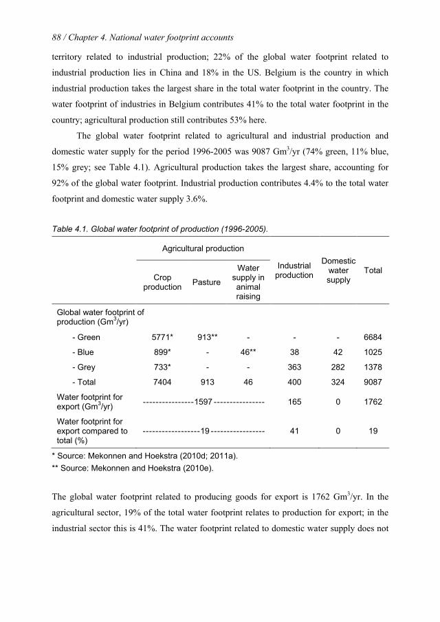
88 / Chapter 4. National water footprint accounts
territory related to industrial production; 22% of the global water footprint related to
industrial production lies in China and 18% in the US. Belgium is the country in which
industrial production takes the largest share in the total water footprint in the country. The
water footprint of industries in Belgium contributes 41% to the total water footprint in the
country; agricultural production still contributes 53% here.
The global water footprint related to agricultural and industrial production and
domestic water supply for the period 1996-2005 was 9087 Gm3/yr (74% green, 11% blue,
15% grey; see Table 4.1). Agricultural production takes the largest share, accounting for
92% of the global water footprint. Industrial production contributes 4.4% to the total water
footprint and domestic water supply 3.6%.
Table 4.1. Global water footprint of production (1996-2005).
Agricultural production
Industrial production
Domestic water supply
Total Crop
production Pasture
Water supply in animal raising
Global water footprint of production (Gm3/yr)
- Green 5771* 913** - - - 6684
- Blue 899* - 46** 38 42 1025
- Grey 733* - - 363 282 1378
- Total 7404 913 46 400 324 9087
Water footprint for export (Gm3/yr) - - - - - - - - - - - - - - - - 1597 - - - - - - - - - - - - - - - - 165 0 1762
Water footprint for export compared to total (%)
- - - - - - - - - - - - - - - - - - 19 - - - - - - - - - - - - - - - - - 41 0 19
* Source: Mekonnen and Hoekstra (2010d; 2011a). ** Source: Mekonnen and Hoekstra (2010e).
The global water footprint related to producing goods for export is 1762 Gm3/yr. In the
agricultural sector, 19% of the total water footprint relates to production for export; in the
industrial sector this is 41%. The water footprint related to domestic water supply does not
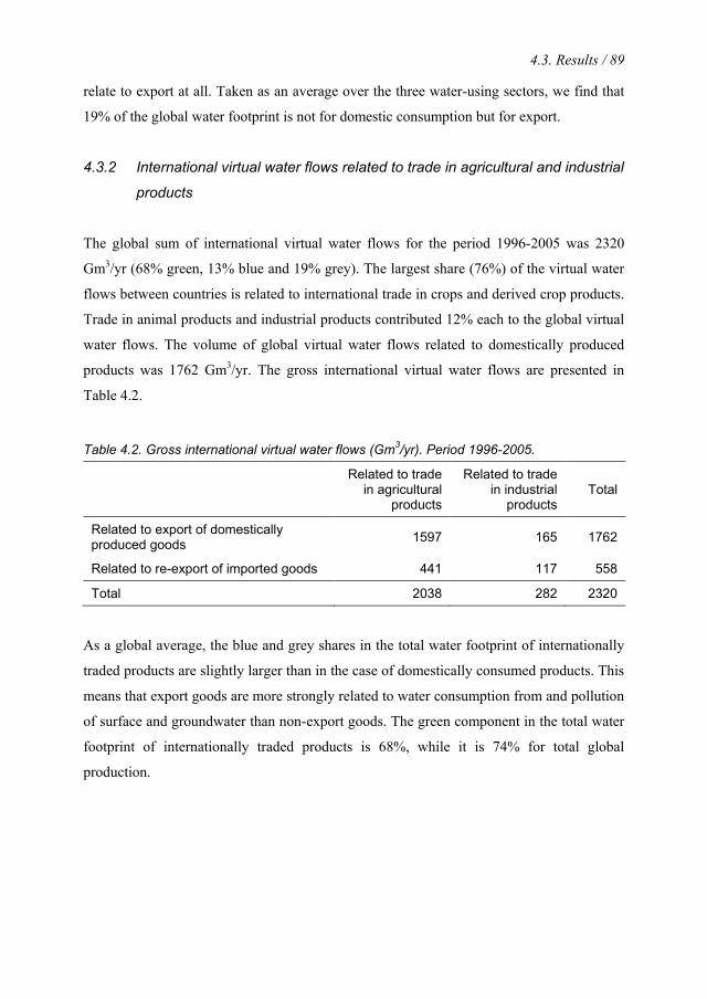
4.3. Results / 89
relate to export at all. Taken as an average over the three water-using sectors, we find that
19% of the global water footprint is not for domestic consumption but for export.
4.3.2 International virtual water flows related to trade in agricultural and industrial
products
The global sum of international virtual water flows for the period 1996-2005 was 2320
Gm3/yr (68% green, 13% blue and 19% grey). The largest share (76%) of the virtual water
flows between countries is related to international trade in crops and derived crop products.
Trade in animal products and industrial products contributed 12% each to the global virtual
water flows. The volume of global virtual water flows related to domestically produced
products was 1762 Gm3/yr. The gross international virtual water flows are presented in
Table 4.2.
Table 4.2. Gross international virtual water flows (Gm3/yr). Period 1996-2005.
Related to trade in agricultural
products
Related to trade in industrial
products Total
Related to export of domestically produced goods 1597 165 1762
Related to re-export of imported goods 441 117 558
Total 2038 282 2320
As a global average, the blue and grey shares in the total water footprint of internationally
traded products are slightly larger than in the case of domestically consumed products. This
means that export goods are more strongly related to water consumption from and pollution
of surface and groundwater than non-export goods. The green component in the total water
footprint of internationally traded products is 68%, while it is 74% for total global
production.
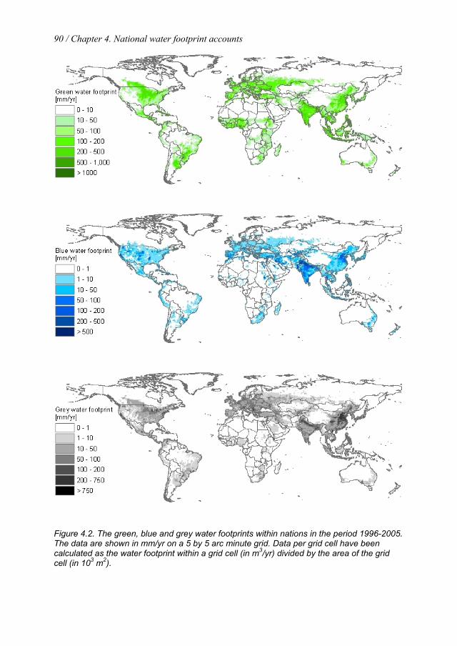
90 / Chapter 4. National water footprint accounts
Figure 4.2. The green, blue and grey water footprints within nations in the period 1996-2005. The data are shown in mm/yr on a 5 by 5 arc minute grid. Data per grid cell have been calculated as the water footprint within a grid cell (in m3/yr) divided by the area of the grid cell (in 103 m2).
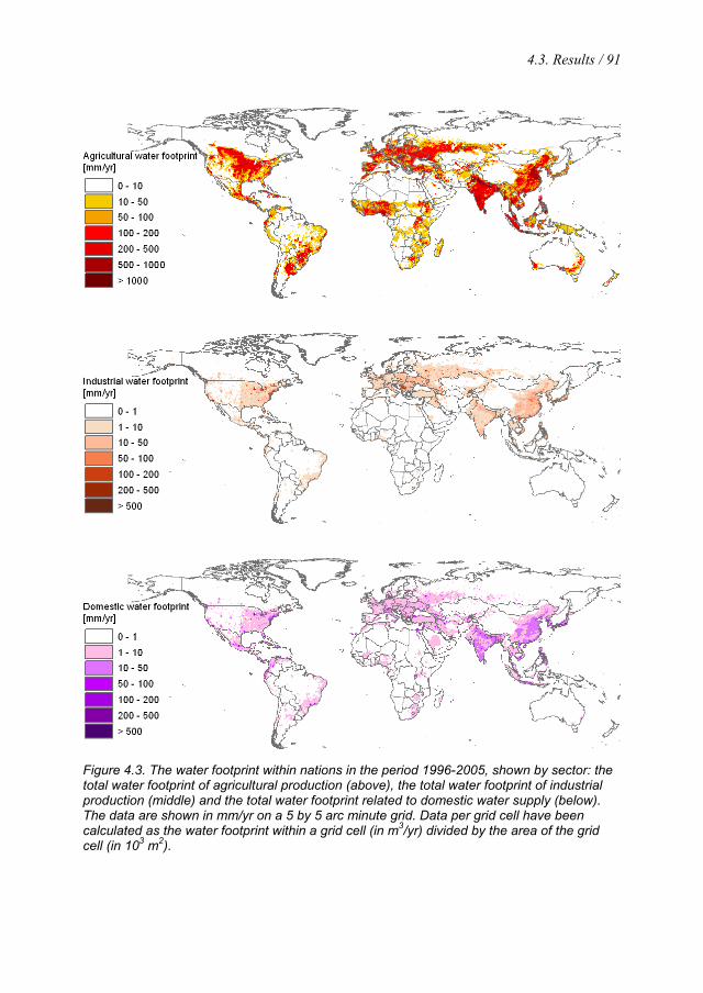
4.3. Results / 91
Figure 4.3. The water footprint within nations in the period 1996-2005, shown by sector: the total water footprint of agricultural production (above), the total water footprint of industrial production (middle) and the total water footprint related to domestic water supply (below). The data are shown in mm/yr on a 5 by 5 arc minute grid. Data per grid cell have been calculated as the water footprint within a grid cell (in m3/yr) divided by the area of the grid cell (in 103 m2).
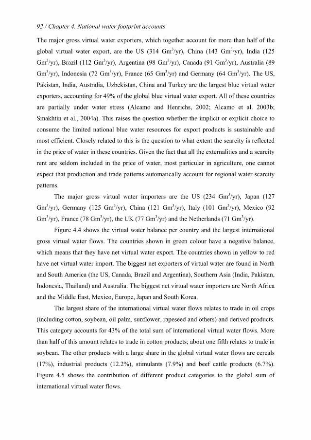
92 / Chapter 4. National water footprint accounts
The major gross virtual water exporters, which together account for more than half of the
global virtual water export, are the US (314 Gm3/yr), China (143 Gm3/yr), India (125
Gm3/yr), Brazil (112 Gm3/yr), Argentina (98 Gm3/yr), Canada (91 Gm3/yr), Australia (89
Gm3/yr), Indonesia (72 Gm3/yr), France (65 Gm3/yr) and Germany (64 Gm3/yr). The US,
Pakistan, India, Australia, Uzbekistan, China and Turkey are the largest blue virtual water
exporters, accounting for 49% of the global blue virtual water export. All of these countries
are partially under water stress (Alcamo and Henrichs, 2002; Alcamo et al. 2003b;
Smakhtin et al., 2004a). This raises the question whether the implicit or explicit choice to
consume the limited national blue water resources for export products is sustainable and
most efficient. Closely related to this is the question to what extent the scarcity is reflected
in the price of water in these countries. Given the fact that all the externalities and a scarcity
rent are seldom included in the price of water, most particular in agriculture, one cannot
expect that production and trade patterns automatically account for regional water scarcity
patterns.
The major gross virtual water importers are the US (234 Gm3/yr), Japan (127
Gm3/yr), Germany (125 Gm3/yr), China (121 Gm3/yr), Italy (101 Gm3/yr), Mexico (92
Gm3/yr), France (78 Gm3/yr), the UK (77 Gm3/yr) and the Netherlands (71 Gm3/yr).
Figure 4.4 shows the virtual water balance per country and the largest international
gross virtual water flows. The countries shown in green colour have a negative balance,
which means that they have net virtual water export. The countries shown in yellow to red
have net virtual water import. The biggest net exporters of virtual water are found in North
and South America (the US, Canada, Brazil and Argentina), Southern Asia (India, Pakistan,
Indonesia, Thailand) and Australia. The biggest net virtual water importers are North Africa
and the Middle East, Mexico, Europe, Japan and South Korea.
The largest share of the international virtual water flows relates to trade in oil crops
(including cotton, soybean, oil palm, sunflower, rapeseed and others) and derived products.
This category accounts for 43% of the total sum of international virtual water flows. More
than half of this amount relates to trade in cotton products; about one fifth relates to trade in
soybean. The other products with a large share in the global virtual water flows are cereals
(17%), industrial products (12.2%), stimulants (7.9%) and beef cattle products (6.7%).
Figure 4.5 shows the contribution of different product categories to the global sum of
international virtual water flows.

4.3. Results / 93
Figure 4.4. Virtual water balance per country and direction of gross virtual water flows related to trade in agricultural and industrial products over the period 1996-2005. Only the biggest gross flows (> 15 Gm3/yr) are shown; the fatter the arrow, the bigger the virtual water flow.
Oilcrops42.7%
Cereals17.0%
Industrial products12.2%
Stimulants7.9%
Bovine products6.7%
Sugarcrops3.5%
Fruits2.0%
Milk products1.6%
Swine products1.5%
Pulses0.8%
Poultry0.8%
Spices0.7%
Horse0.5%
Nuts0.5% Sheep
0.5%
Roots and Tubers0.3%
Tobacco0.2%
Other0.5%
Other6.4%
Figure 4.5. Contribution of different product categories to the global virtual water flows
4.3.3 National water saving per country as a result of trade
A number of countries reduce the use of their national water resources through the import
of agricultural products. Japan saves 134 Gm3/yr (80% green, 9% blue, 12% grey) of its
domestic water resources, Mexico 83 Gm3/yr (69% green, 26% blue, 6% grey), Italy 54
Gm3/yr (83% green, 10% blue, 7% grey), the UK 53 Gm3/yr (75% green, 15% blue, 9%
94 / Chapter 4. National water footprint accounts
grey) and Germany 50 Gm3/yr (83% green, 14% blue, 3% grey). In terms of blue water
saved, Mexico, Spain, Japan, the UK and a number of countries in the Middle East come on
top of the list. The figures on ‘national water saving’ presented here should be merely
understood as ‘volumes of domestic water resources not necessary to be used for
production because the commodities are imported’. The term ‘saving’ is used in a physical,
not economic sense. Besides, the ‘water saving’ does not necessarily imply that the water
saved is allocated to other beneficial uses (De Fraiture et al. 2004). In water-scarce
countries, however, ‘water saving’ is likely to have positive environmental, social and
economic implications.
From a water resources point of view, one would expect that countries facing water
stress adopt a trade strategy that alleviates their water scarcity problem. However,
international trade in agricultural goods is driven largely by factors other than water.
Therefore, import of virtual water is often unrelated to relative water scarcity in a country
(Yang et al., 2003; De Fraiture et al., 2004; Oki and Kanae, 2004; Chapagain and Hoekstra,
2008; Yang and Zehnder, 2008). As shown by Yang et al. (2003), only below a certain
threshold in water availability can a relationship be established between the country’s per
capita water availability and its cereal import. For most relatively water-scarce countries –
like in North Africa, Middle East, Southern Europe and Mexico – we find indeed net virtual
water imports and related national water savings. The national water savings found for
Northern European countries, however, cannot be understood from a water scarcity
perspective.
4.3.4 Global water saving related to trade in agricultural and industrial products
The global water saving related to trade in agricultural products in the period 1996-2005
was 369 Gm3/yr (58.7% green, 26.6% blue and 14.7% grey). This volume is equivalent to
4% of the global water footprint related to agricultural production (which is 8363 Gm3/yr,
see Table 4.1). Looking only at the blue water saving, it would have required an additional
98 Gm3/yr of blue water to produce the same amount of goods without virtual water trade.
This volume is equivalent to 10% of the global blue water footprint related to agricultural
production (which is 945 Gm3/yr, see again Table 4.1). More than a quarter (98/369=27%)
of the global water saving related to agricultural trade is blue water, which indicates that
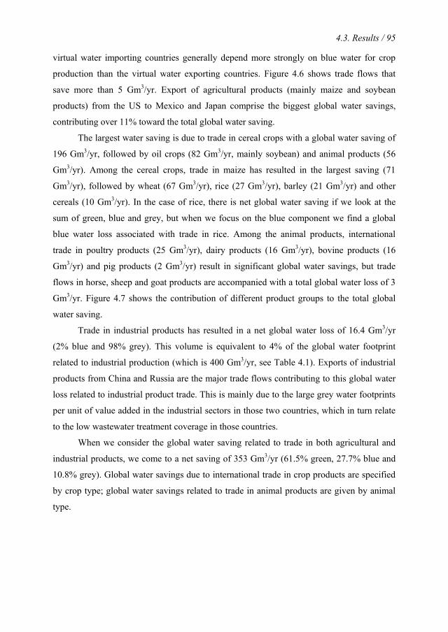
4.3. Results / 95
virtual water importing countries generally depend more strongly on blue water for crop
production than the virtual water exporting countries. Figure 4.6 shows trade flows that
save more than 5 Gm3/yr. Export of agricultural products (mainly maize and soybean
products) from the US to Mexico and Japan comprise the biggest global water savings,
contributing over 11% toward the total global water saving.
The largest water saving is due to trade in cereal crops with a global water saving of
196 Gm3/yr, followed by oil crops (82 Gm3/yr, mainly soybean) and animal products (56
Gm3/yr). Among the cereal crops, trade in maize has resulted in the largest saving (71
Gm3/yr), followed by wheat (67 Gm3/yr), rice (27 Gm3/yr), barley (21 Gm3/yr) and other
cereals (10 Gm3/yr). In the case of rice, there is net global water saving if we look at the
sum of green, blue and grey, but when we focus on the blue component we find a global
blue water loss associated with trade in rice. Among the animal products, international
trade in poultry products (25 Gm3/yr), dairy products (16 Gm3/yr), bovine products (16
Gm3/yr) and pig products (2 Gm3/yr) result in significant global water savings, but trade
flows in horse, sheep and goat products are accompanied with a total global water loss of 3
Gm3/yr. Figure 4.7 shows the contribution of different product groups to the total global
water saving.
Trade in industrial products has resulted in a net global water loss of 16.4 Gm3/yr
(2% blue and 98% grey). This volume is equivalent to 4% of the global water footprint
related to industrial production (which is 400 Gm3/yr, see Table 4.1). Exports of industrial
products from China and Russia are the major trade flows contributing to this global water
loss related to industrial product trade. This is mainly due to the large grey water footprints
per unit of value added in the industrial sectors in those two countries, which in turn relate
to the low wastewater treatment coverage in those countries.
When we consider the global water saving related to trade in both agricultural and
industrial products, we come to a net saving of 353 Gm3/yr (61.5% green, 27.7% blue and
10.8% grey). Global water savings due to international trade in crop products are specified
by crop type; global water savings related to trade in animal products are given by animal
type.
96 / Chapter 4. National water footprint accounts
7.4 Gm3/yr
7.8 Gm3/yr9.3
Gm3/yr
25 Gm3/yr
5.6 Gm3/yr5.4
Gm3/yr
12 Gm3/yr
5.0 Gm3/yr
5.7 Gm3/yr
5.1 Gm3/yr
16 Gm3/yr
5.0 Gm3/yr
89%
5% 6%
85%
14%-1%
54%
45%
1%60%
37%
-3%
77%
17%6%
40%
50%
-10%
85%
13%-2%
38%32%
-30%
21%
73%
-6%
Green
Blue
Grey
85%
- 3%-12%
71%-5%
24%
83%
8%-9%
Figure 4.6.Global water savings associated with international trade in agricultural products (1996-2005). Only the biggest water savings (> 5 Gm3/yr) are shown.

4.3. Results / 97
-50
0
50
100
150
200
250
Cereals Oilcrops Animals products Fruits Other crops
Glo
bal w
ater
savi
ng (G
m3 /y
r)
Green Blue Grey
196
82
56
13 22Industrial
-16
-10
0
10
20
30 Poultry 25
Dairy 16
Bovine 16
Others -1
-20
0
20
40
60
80Maize
71 Wheat 67
Rice 27 Barley
21Others
10
-40
-20
0
20
40
60
80 Soybeans 60
Others 21
Figure 4.7. Contribution of different product categories to the total global water saving (1996-2005).
The calculated trade-related water savings are based on the crop yields and corresponding
water footprints as they currently exist in the exporting and importing countries. One
should therefore be careful in extrapolating water savings when trade flows would
intensify. Water scarcity will stimulate countries to improve their water productivities,
particularly in countries with low yields (Appelgren and Klohn, 1999; Keller et al., 1998;
Molle, 2003; Ohlsson, 2000). Current global water savings resulting from trade in water-
intensive products from countries with high water productivity to countries with low water
productivity will diminish once the latter countries have increased their water productivity.
The presented global water saving related to international trade may seem
significant: the global water footprint of agricultural and industrial production would be 4%
higher if countries would produce all commodities within their own territory based on
existing domestic productivities instead of partially import them from other countries. The
potential of optimising international trade for further global water savings is probably small
once the most important importing countries with low water productivities increase their
productivity. The global water footprint can be reduced more significantly by achieving
high water productivities across the globe than by optimising trade from high to low
productivity regions. Supported by the assessment by Falkenmark et al. (2009), we estimate
that the potential global water saving by increasing water productivities in regions that
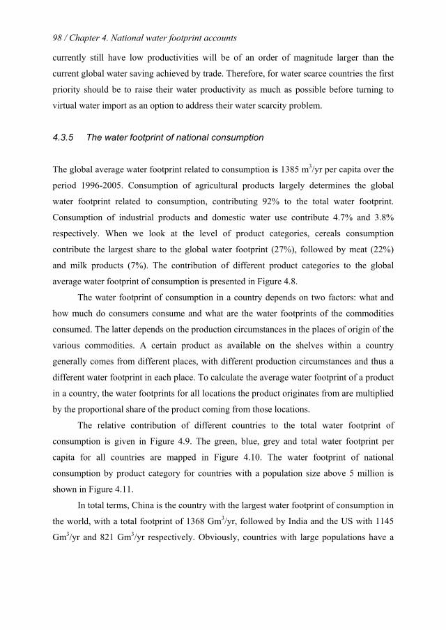
98 / Chapter 4. National water footprint accounts
currently still have low productivities will be of an order of magnitude larger than the
current global water saving achieved by trade. Therefore, for water scarce countries the first
priority should be to raise their water productivity as much as possible before turning to
virtual water import as an option to address their water scarcity problem.
4.3.5 The water footprint of national consumption
The global average water footprint related to consumption is 1385 m3/yr per capita over the
period 1996-2005. Consumption of agricultural products largely determines the global
water footprint related to consumption, contributing 92% to the total water footprint.
Consumption of industrial products and domestic water use contribute 4.7% and 3.8%
respectively. When we look at the level of product categories, cereals consumption
contribute the largest share to the global water footprint (27%), followed by meat (22%)
and milk products (7%). The contribution of different product categories to the global
average water footprint of consumption is presented in Figure 4.8.
The water footprint of consumption in a country depends on two factors: what and
how much do consumers consume and what are the water footprints of the commodities
consumed. The latter depends on the production circumstances in the places of origin of the
various commodities. A certain product as available on the shelves within a country
generally comes from different places, with different production circumstances and thus a
different water footprint in each place. To calculate the average water footprint of a product
in a country, the water footprints for all locations the product originates from are multiplied
by the proportional share of the product coming from those locations.
The relative contribution of different countries to the total water footprint of
consumption is given in Figure 4.9. The green, blue, grey and total water footprint per
capita for all countries are mapped in Figure 4.10. The water footprint of national
consumption by product category for countries with a population size above 5 million is
shown in Figure 4.11.
In total terms, China is the country with the largest water footprint of consumption in
the world, with a total footprint of 1368 Gm3/yr, followed by India and the US with 1145
Gm3/yr and 821 Gm3/yr respectively. Obviously, countries with large populations have a
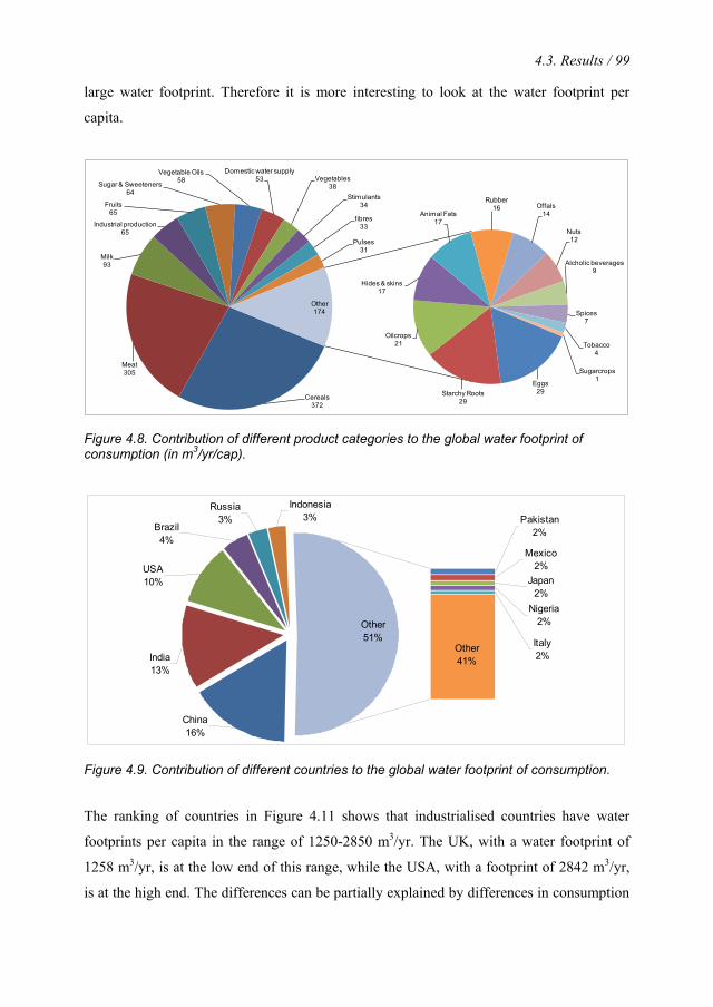
4.3. Results / 99
large water footprint. Therefore it is more interesting to look at the water footprint per
capita.
Cereals372
Meat305
Milk93
Industrial production65
Fruits 65
Sugar & Sweeteners 64
Vegetable Oils58
Domestic water supply53 Vegetables
38Stimulants
34
fibres33
Pulses31
Eggs29Starchy Roots
29
Oilcrops21
Hides & skins17
Animal Fats17
Rubber16 Offals
14
Nuts12
Alcholic beverages9
Spices 7
Tobacco4
Sugarcrops1
Other174
Figure 4.8. Contribution of different product categories to the global water footprint of consumption (in m3/yr/cap).
Other51%
China16%
India13%
USA10%
Brazil4%
Russia3%
Indonesia3% Pakistan
2%
Mexico2%
Japan2%
Nigeria2%
Italy2%
Other41%
Figure 4.9. Contribution of different countries to the global water footprint of consumption.
The ranking of countries in Figure 4.11 shows that industrialised countries have water
footprints per capita in the range of 1250-2850 m3/yr. The UK, with a water footprint of
1258 m3/yr, is at the low end of this range, while the USA, with a footprint of 2842 m3/yr,
is at the high end. The differences can be partially explained by differences in consumption

100 / Chapter 4. National water footprint accounts
pattern. In the USA, for example, average consumption of bovine meat – one of the highly
water-intensive commodities – was 43 kg/yr per capita, about 4.5 times the global average,
while in the UK this was 18 kg/yr per capita, about two times the global average. Another
factor behind the differences in the water footprints is the water consumption and pollution
per unit of product per country. In the USA, the average water footprint of one kg of
consumed bovine meat is 14500 m3/ton, while in the UK this is 9900 m3/ton.
The water footprint per capita for developing countries varies much more than for
industrialised countries. We find values in a range 550-3800 m3/yr per capita. At the low
end is the Democratic Republic of Congo, with 552 m3/yr per capita. At the high end we
find Bolivia (3468 m3/yr/cap), Niger (3519 m3/yr/cap) and Mongolia (3775 m3/yr/cap).
With the disclaimer that the extreme values can also partially relate to weak basic data on
consumption and water productivity in those countries, the differences can be traced back
to differences in consumptions patterns on the one hand and differences in the water
footprints of the products consumed on the other hand. What the ranking in Figure 4.11
shows is that in the range of relatively large water footprints per capita we find both
industrialised and developing countries. The latter are in that range generally not because of
their relatively large consumption – although relatively large meat consumption can play a
role – but because of their low water productivities, i.e. large water footprints per ton of
product consumed. In Bolivia, for example, consumption of meat is 1.3 times the global
average, but the water footprint per ton of meat is five times the global average. For Niger,
the consumption of cereals per capita is 1.4 times the global average, but the water footprint
of cereals per ton is six times the world average.
When we look at the blue water footprint per capita, countries in Central and
Southwest Asia and North Africa appear on top. Consumers in Turkmenistan have the
largest blue water footprint of all countries, namely 740 m3/yr per capita on average. Other
countries with a large blue water footprint are (in descending order): Iran (589 m3/yr/cap),
the United Arab Emirates (571), Egypt (527), Libya (511), Tajikistan (474), Saudi Arabia
(447) and Pakistan (422). The global average blue water footprint of consumption is 153
m3/yr per capita, which is 11% of the total water footprint. As can be seen in Figure 4.12,
the variation in blue water footprint per capita across countries is huge, much larger than
the variation in total water footprint per capita (Figure 4.11). Whereas the largest total
water footprint per capita (Mongolia) is about seven times the smallest total water footprint
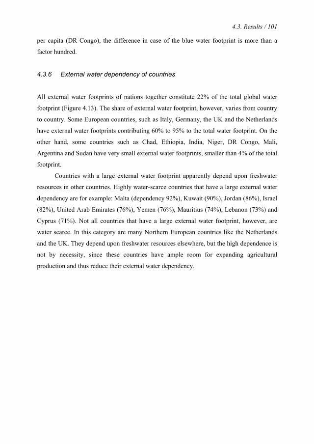
4.3. Results / 101
per capita (DR Congo), the difference in case of the blue water footprint is more than a
factor hundred.
4.3.6 External water dependency of countries
All external water footprints of nations together constitute 22% of the total global water
footprint (Figure 4.13). The share of external water footprint, however, varies from country
to country. Some European countries, such as Italy, Germany, the UK and the Netherlands
have external water footprints contributing 60% to 95% to the total water footprint. On the
other hand, some countries such as Chad, Ethiopia, India, Niger, DR Congo, Mali,
Argentina and Sudan have very small external water footprints, smaller than 4% of the total
footprint.
Countries with a large external water footprint apparently depend upon freshwater
resources in other countries. Highly water-scarce countries that have a large external water
dependency are for example: Malta (dependency 92%), Kuwait (90%), Jordan (86%), Israel
(82%), United Arab Emirates (76%), Yemen (76%), Mauritius (74%), Lebanon (73%) and
Cyprus (71%). Not all countries that have a large external water footprint, however, are
water scarce. In this category are many Northern European countries like the Netherlands
and the UK. They depend upon freshwater resources elsewhere, but the high dependence is
not by necessity, since these countries have ample room for expanding agricultural
production and thus reduce their external water dependency.
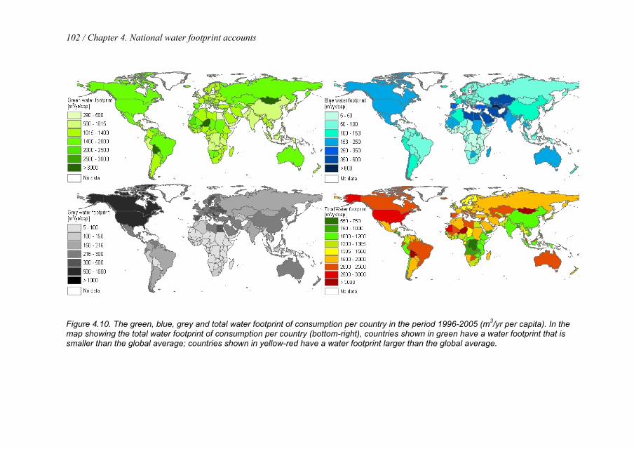
102 / Chapter 4. National water footprint accounts
Figure 4.10. The green, blue, grey and total water footprint of consumption per country in the period 1996-2005 (m3/yr per capita). In the map showing the total water footprint of consumption per country (bottom-right), countries shown in green have a water footprint that is smaller than the global average; countries shown in yellow-red have a water footprint larger than the global average.

4.3. Results / 103
0
500
1000
1500
2000
2500
3000
3500
Congo, D
RB
urundiB
angladeshR
wanda
Korea, D
PR
Yemen
Nicaragua
Zambia
Malaw
iA
ngolaG
uatemala
TogoTanzaniaH
aitiE
l Salvador
LaosV
iet Nam
China
Cam
bodiaU
gandaP
eruIndiaK
enyaM
ozambique
IndonesiaB
eninS
enegalC
hileE
thiopiaH
ondurasN
epalG
hanaZim
babwe
Myanm
arN
igeriaA
zerbaijanC
ameroon
South A
fricaS
ri LankaU
KU
zbekistanC
ôte d'IvoireP
akistanS
lovakiaE
gyptC
olombia
Philippines
JapanD
ominican R
epP
olandThailandFinlandG
ermany
Sw
edenC
hadN
etherlandsS
witzerland
Ukraine
Madagascar
Algeria
Austria
Guinea
Argentina
Korea, R
epD
enmark
TurkeyC
zech Republic
Cuba
Rom
aniaB
urkina FasoV
enezuelaB
elarusM
oroccoS
udanFranceS
audi Arabia
Russia
IranB
elgiumP
araguayM
exicoE
cuadorB
razilLibyaM
aliM
alaysiaS
yriaTunisiaB
ulgariaIsraelItalyA
ustraliaC
anadaG
reeceK
azakhstanH
ungaryTajikistanS
erbia & M
ontenegroS
painP
ortugalU
SA
Bolivia
Niger
World average
Cereals Starchy Roots Sugarcrops Sugar & Sweeteners Pulses Nuts Oilcrops Vegetable Oils
Vegetables Fruits Stimulants Spices Wine & beer fibres Tobacco Rubber
Meat Offals Animal Fats Milk Eggs Hides & skins Industrial products Domestic water supply
Figure 4.11. Water footprint of national consumption for countries with a population larger than 5 million, shown by product category (m3/yr/cap) (1996-2005).
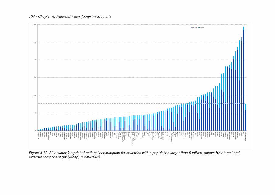
104 / Chapter 4. National water footprint accounts
0
100
200
300
400
500
600
Congo, D
RR
wanda
Uganda
Burundi
Malaw
iM
ozambique
TogoB
eninC
hadN
igeriaG
hanaE
thiopiaA
ngolaB
urkina FasoC
ameroon
Guinea
Guatem
alaK
enyaTanzaniaZam
biaM
yanmar
Côte d'Ivoire
Honduras
Nicaragua
El S
alvadorP
araguayU
kraineP
olandC
ambodia
Bolivia
Belarus
Hungary
Colom
biaZim
babwe
Brazil
LaosIndonesiaS
lovakiaH
aitiR
omania
Philippines
FinlandC
zech Republic
Bangladesh
Sw
edenB
ulgariaG
ermany
Serbia &
Montenegro
Korea, D
PR
Senegal
Niger
Venezuela
Viet N
amJapanU
KR
ussiaD
enmark
South A
fricaA
ustriaC
ubaA
rgentinaK
orea, Rep
Sw
itzerlandC
hinaN
epalN
etherlandsD
ominican R
epFranceB
elgiumA
lgeriaE
cuadorP
eruM
alaysiaC
anadaM
aliS
ri LankaM
adagascarThailandC
hileM
exicoItalyA
zerbaijanS
udanM
oroccoA
ustraliaYem
enIndiaU
SA
TurkeyIsraelTunisiaS
painG
reeceP
ortugalU
zbekistanK
azakhstanS
yriaP
akistanS
audi Arabia
TajikistanLibyaE
gyptIranW
orld averageInternal External
Figure 4.12. Blue water footprint of national consumption for countries with a population larger than 5 million, shown by internal and external component (m3/yr/cap) (1996-2005).
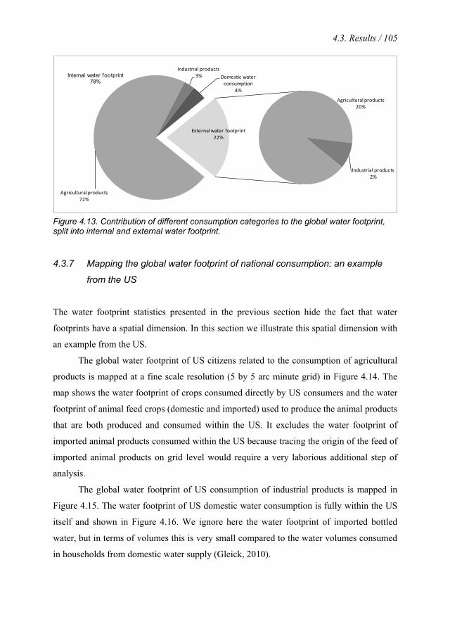
4.3. Results / 105
Agricultural products72%
Industrial products3% Domestic water
consumption4%
Agricultural products 20%
Industrial products2%
External water footprint 22%
Internal water footprint 78%
Figure 4.13. Contribution of different consumption categories to the global water footprint, split into internal and external water footprint.
4.3.7 Mapping the global water footprint of national consumption: an example
from the US
The water footprint statistics presented in the previous section hide the fact that water
footprints have a spatial dimension. In this section we illustrate this spatial dimension with
an example from the US.
The global water footprint of US citizens related to the consumption of agricultural
products is mapped at a fine scale resolution (5 by 5 arc minute grid) in Figure 4.14. The
map shows the water footprint of crops consumed directly by US consumers and the water
footprint of animal feed crops (domestic and imported) used to produce the animal products
that are both produced and consumed within the US. It excludes the water footprint of
imported animal products consumed within the US because tracing the origin of the feed of
imported animal products on grid level would require a very laborious additional step of
analysis.
The global water footprint of US consumption of industrial products is mapped in
Figure 4.15. The water footprint of US domestic water consumption is fully within the US
itself and shown in Figure 4.16. We ignore here the water footprint of imported bottled
water, but in terms of volumes this is very small compared to the water volumes consumed
in households from domestic water supply (Gleick, 2010).
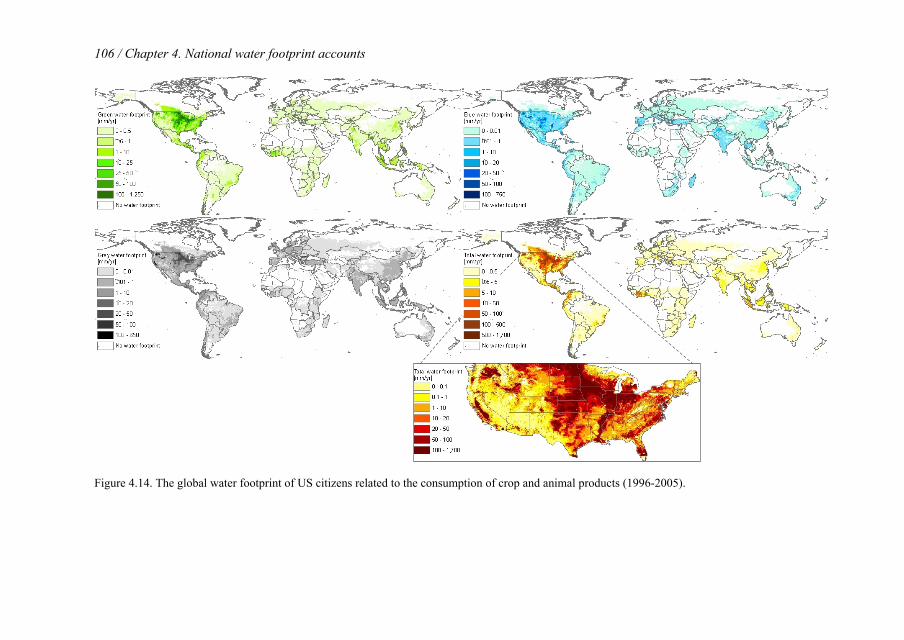
106 / Chapter 4. National water footprint accounts
Figure 4.14. The global water footprint of US citizens related to the consumption of crop and animal products (1996-2005).

4.3. Results / 107
Figure 4.15. The global water footprint of US citizens related to the consumption of industrial products (1996-2005).

108 / Chapter 4. National water footprint accounts
Figure 4.16. The water footprint of US citizens related to domestic water supply (1996-2005). The boundaries shown are river basin boundaries.
Most of the US water footprint lies within the US, mainly in the Mississippi basin (more
than 50%). About 20% of the water footprint of US citizens lies outside the US. The largest
water footprint outside the US is in the Yangtze basin (China).
4.4. Discussion / 109
4.4 Discussion
The global water footprint related to agricultural and industrial production and domestic
water supply for the period 1996-2005 was found to be 9087 Gm3/yr (Section 4.3.1). If we
calculate the global sum of estimated national water footprints of consumption (Section
4.3.5), we arrive at a 6% lower figure, namely 8525 Gm3/yr. An explanation is that the
latter figure is conservative, because in the estimation of the water footprint of national
consumption of agricultural products based on the bottom-up approach we only partially
accounted for the water footprint of waste and seeds. We multiplied all consumption figures
by a certain factor to account for waste and seeds where applicable (see method and data
section) for all crop and animal products consumed but we could not account for the water
footprint of waste and seeds in the production of animal feed. Another reason for the
difference between the two global water footprint estimates is that in the water footprint of
global production we could account for all countries, while in the estimation of the water
footprint of national consumption we had to exclude a few countries due to the absence of
consumption data (most notably Iraq and Afghanistan). Another explanation of the
difference is that in the estimation of the national water footprint related to consumption we
could not include all consumer categories (like for example some alcoholic beverages).
When it was not clear which crops underlie certain products, we could not calculate the
water footprint per ton of those products. A final explanation for differences between the
two global water footprint figures could be that stock changes reported in the Supply and
Utilization Accounts of the Food and Agriculture Organization (FAO, 2010a) create a
difference between ‘production plus imports’ and ‘utilization’ in a certain period.
This study is the first to use the bottom-up approach to estimate the water footprint
of national consumption of agricultural commodities at a global scale. As shown by Van
Oel et al. (2009), the advantage of using the bottom-up approach is that it is more stable.
The bottom-up approach depends on the quality of consumption data, while the top-down-
approach relies on the quality of production and trade data. The outcome of the top-down
approach can be vulnerable to relatively small errors in the trade data when the import and
export of a country are large relative to its domestic production. Relatively small errors in
the estimates of virtual-water import and export can then translate into a relatively large
error in the water footprint estimate. In such a case, the bottom-up approach yields a more
110 / Chapter 4. National water footprint accounts
reliable estimate than the top-down approach. Another advantage of the bottom-up
approach is that it allows for showing the composition of the water footprint by commodity
or product category in a very straightforward manner (because this is the way the overall
estimate is built up), which in the top-down approach is difficult to achieve.
A limitation in the study is that the origin of products has been traced only by one
step. If a product is imported from another country, we assume that the product has been
produced in that country and we take the water footprint of the imported product
accordingly. If the trade partner country does not produce that commodity, we do not trace
further back but assume a global average water footprint. But even if the country produces
the product, it could have been the case that the product was in part imported from
somewhere else and re-exported. Tracing of products by more than one step has been done
for example by Chapagain and Orr (2008) for the UK but this was too laborious for this
global study. Besides, such continued tracing effort is necessarily based on assumptions
because export data in trade statistics are not connected to import data, therefore the added
value of tracing can be questioned. Finally, in a global study, tracing back more than one
step would create the problem of circularity in the calculations. Common products are
traded in all directions between all countries, so that a strategy of tracing products will soon
lead to the situation in which a small fraction of a product imported to a country X is
estimated to originate, through a detour, from the same country X. This leads to a
mathematical circularity in the calculation of the average water footprint of the product in
country X – see equation (17).
The grey water footprint estimates in this study are to be considered as conservative.
In the case of agricultural production, the grey water footprint estimates are based on
leaching and runoff of nitrogen fertilisers, excluding the potential effect of other fertiliser
components and pesticides (Mekonnen and Hoekstra, 2010d, 2011a). In the cases of
industrial production and domestic water supply, a very conservative dilution factor of 1
has been applied for all untreated return flows.
While in the estimation of the water footprint of consumer products we considered a
huge amount of different agricultural commodities separately, industrial commodities were
treated as one whole category. Although in this way the study shows no detail within the
estimation of the water footprint of production and consumption of industrial products, we
4.5. Conclusion / 111
justify the choice in this global study based on the fact that most of the water footprint of
humanity is within the agricultural sector.
We have analysed a ten-year period, but we do not show annual variations or trends
in time. The reason is that the data do not allow for that. Many of the databases that we
used show data for every individual year within our ten-year period (e.g. production,
consumption, trade, rainfall and yield data), but not all global databases show year-specific
data (e.g. reference evapotranspiration, crop growing area and irrigation data). The
estimated water footprints of agricultural products are necessarily ten-year averages,
because they have been based on climate data, which are by definition multi-year averages
(Mekonnen and Hoekstra, 2010d, 2011a). Even if we would have been able to estimate
water footprints by year, a trend analysis over a ten-year period would have been difficult
due to the natural inter-annual variability of rainfall and temperature.
The data presented in this paper are derived on the basis of a great number of
underlying statistics, maps and assumptions. Since all basic sources include uncertainties
and possible errors, the presented water footprint data should be taken and interpreted with
extreme caution, particularly when zooming in on specific locations on a map or when
focussing on specific products. Basic sources of uncertainties are for example the global
precipitation, temperature, crop and irrigation maps that we have used and the yield,
production, consumption, trade and wastewater treatment statistics that we had to rely on.
Underlying assumptions refer, for example, to planting and harvesting dates per crop per
region and feed composition per farm animal type per country and production system.
Another assumption has been that water footprints of industrial production and domestic
water supply are geographically spread according to population densities. Despite the
plethora of uncertainties, we think that the current study forms a good basis for rough
comparisons and to guide further analysis.
4.5 Conclusion
The study shows that about one fifth of the global water footprint in the period 1996-2005
was not related to production for domestic consumption but for export. The global volume
of water saving from international trade in agricultural products was equivalent to 4% of
the global water footprint for agricultural production. The relatively large volume of

112 / Chapter 4. National water footprint accounts
international virtual water flows and the associated national water savings and external
water dependencies strengthen the argument to consider issues of local water scarcity in a
global context (Hoekstra and Chapagain, 2008; Hoekstra, 2011).
Two factors determine the magnitude of the water footprint of national consumption:
(1) the volume and pattern of consumption and (2) the water footprint per ton of consumed
products. The latter, in the case of agricultural products, depends on climate, irrigation and
fertilization practice and crop yield. The global average water footprint related to
consumption is 1385 m3/yr per capita over the period 1996-2005. Industrialised countries
have water footprints in the range of 1250-2850 m3/yr/cap, while developing countries
show a much larger range of 550-3800 m3/yr/cap. The low values for developing countries
relate to low consumption volumes; the large values refer to very large water footprints per
unit of consumption.
The study provides important information on the water footprints of nations,
disaggregated into the type of water footprint (green, blue or grey) and mapped at a high
spatial resolution. The paper shows how different products and national communities
contribute to water consumption and pollution in different places. The figures can thus form
an important basis for further assessment of how products and consumers contribute to the
global problem of increasing freshwater appropriation against the background of limited
supplies and to local problems of overexploitation and deterioration of freshwater bodies or
conflict over water. Once one starts overlaying localised water footprints of products or
consumers with maps that show environmental or social water conflict, a link has been
established between final products and consumers on the one hand and local water
problems on the other hand. Establishing such links can help the dialogue between
consumers, producers, intermediates (like food processors and retailers) and governments
about how to share responsibility for reducing water footprints where most necessary.
5. Global water scarcity: The monthly blue water footprint compared to blue water availability for the world’s major river basins4
Abstract
Conventional blue water scarcity indicators suffer from four weaknesses: they measure
water withdrawal instead of consumptive water use, they compare water use with actual
runoff rather than natural (undepleted) runoff, they ignore environmental flow requirements
and they evaluate scarcity on an annual rather than a monthly time scale. In the current
study, these shortcomings are solved by defining blue water scarcity as the ratio of blue
water footprint to blue water availability – where the latter is taken as natural runoff minus
environmental flow requirement – and by estimating all underlying variables on a monthly
basis.
The objective of this study is to assess the intra-annual variability of blue water
scarcity for the world’s major river basins. Monthly blue water footprints were estimated
based on Mekonnen and Hoekstra (2011b). Natural runoff per river basin was estimated by
adding estimates of actual runoff from Fekete et al. (2002) and estimates of water volumes
already consumed. Environmental flow requirements were estimated based on the
presumptive standard for environmental flow protection as proposed by Richter et al.
(2011), which can be regarded as a precautionary estimate of environmental flow
requirements.
Within the study period 1996-2005, in 223 river basins (55% of the basins studied)
with in total 2.72 billion inhabitants (69% of the total population living in the basins
included in this study), the blue water scarcity level exceeded one hundred per cent during
at least one month of the year, which means that environmental flow requirements were
violated during at least one month of the year. In 201 river basins with in total 2.67 billion
people there was severe water scarcity during at least one month per year, which means that
the blue water footprint was more than twice the blue water availability during at least one
month per year.
4 Based on Hoekstra and Mekonnen (2011)
114 / Chapter 5. Global blue water scarcity
Global average blue water scarcity – estimated by averaging the annual average monthly
blue water scarcity values per river basin weighted by basin area – is 85%. This is the
average blue water scarcity over the year within the total land area considered in this study.
When we weight the annual average monthly blue water scarcity values per river basin
according to population number per basin, global average blue water scarcity is 133%. This
is the average scarcity as experienced by the people in the world. This population-weighted
average scarcity is higher than the area-weighted scarcity because the water scarcity values
in densely populated areas – which are often higher than in sparsely populated areas – get
more weight. Yet another way of expressing water scarcity is to take the perspective of the
average water consumer. The global water consumption pattern is different from the
population density pattern, because intensive water consumption in agriculture is not
specifically related to where most people live. If we estimate global blue water scarcity by
averaging monthly blue water scarcity values per river basin weighted based on the blue
water footprint in the respective month and basin, we calculate a global blue water scarcity
at 244%. This means that the average blue water consumer in the world experiences a
water scarcity of 244%, i.e. operates in a month in a basin in which the blue water footprint
is 2.44 times the blue water availability and in which presumptive environmental flow
requirements are thus strongly violated.
5.1 Introduction
Water is a ubiquitous natural resource covering approximately three-quarters of the Earth’s
surface, but 97.5 per cent of the water on the planet is saline water (Shiklomanov and
Rodda, 2003). Only 2.5 per cent of the global water stock is fresh water, but more than two-
thirds of that is locked in the form of ice and snow in the Antarctic, Greenland, arctic
islands and mountainous regions. This leaves less than one per cent of the global water
resources as freshwater accessible for meeting human needs. Fortunately, however,
freshwater is a renewable resource, which means that it is continually replenished through
precipitation over land. Renewable, though, does not mean that supply is unlimited. The
availability of freshwater is primarily limited by the replenishment rate, not by the existing
stocks. Moreover, availability is strongly dependent upon location and time. Globally and
on an annual basis there is enough freshwater to meet human needs but the problem is that
5.1. Introduction / 115
its spatial and temporal distribution is uneven. Spatial and temporal variation of freshwater
availability is often a major determining factor for water scarcity (Postel et al., 1996;
Savenije, 2000).
There have been various studies developing water-scarcity indicators and assessing
global water scarcity. Water-scarcity indicators are always based on two basic ingredients:
a measure of water demand or use and a measure of water availability. One commonly used
indicator of water scarcity is population of an area divided by total runoff in that area,
called the water competition level (Falkenmark, 1989; Falkenmark et al., 1989) or water
dependency (Kulshreshtha, 1993). Many authors take the inverse ratio, thus getting a
measure of the per capita water availability. Falkenmark proposes to consider regions with
more than 1700 m3 per year per capita as ‘water sufficient’, which means that only general
water management problems occur. Between 1000-1700 m3/yr per capita would indicate
‘water stress’, 500-1000 m3/yr ‘chronic water scarcity’ and less than 500 m3/yr ‘absolute
water scarcity’. This classification is based on the idea that 1700 m3 of water per year per
capita is sufficient to produce the food and other goods and services consumed by one
person. This approach ignores the fact that water resources in a certain area do not
necessarily need to be sufficient to feed the people in the area, since people can also import
food (Hoekstra and Hung, 2005). Falkenmark’s water scarcity indicator is not related to the
actual consumption of the people in an area, nor to the efficiency of water use or the way in
which the people obtain their water-intensive goods (through self-production or import).
When the production of water-intensive goods for the people in a country is for a
significant part localised abroad, it may well happen that a country with much less than
1700 m3/yr per capita does not experience serious water problems. And 1700 m3/yr per
capita means much more in a country that uses it water in a highly efficient way and has
reduced demand than in an inefficient country that lacks any demand management.
Another common indicator of water scarcity is the ratio of annual water use in a
certain area to total annual runoff in that area, called variously the water utilization level
(Falkenmark, 1989; Falkenmark et al., 1989), the use-availability ratio (Kulshreshtha,
1993), withdrawal-to-availability ratio (Alcamo and Henrichs, 2002; Oki and Kanae, 2006;
Vörösmarty et al., 2000), use-to-resource ratio (Raskin et al., 1996) or criticality ratio
(Alcamo et al., 1997, 2000; Cosgrove and Rijsberman, 2000a, 200b). As a measure of water
use, the total water withdrawal is taken. There are four critiques to this approach. First,

116 / Chapter 5. Global blue water scarcity
water withdrawal is not the best indicator of water use when one is interested in the effect
of the withdrawal at the scale of the catchment as a whole, because water withdrawals
partly return to the catchment (Perry, 2007). Therefore it makes more sense to express blue
water use in terms of consumptive water use, i.e. by considering the blue water footprint
(Hoekstra et al., 2011). Second, total runoff is not the best indicator of water availability,
because it ignores the fact that part of the runoff needs to be maintained for the
environment. Therefore it is better to subtract the environmental flow requirement from
total runoff (Smakhtin et al., 2004a; Poff et al., 2010). Third, comparing water use to actual
runoff from a catchment becomes problematic when runoff has been substantially lowered
due to the water use within the catchment. It makes more sense to compare water use to
natural or undepleted runoff from the catchment, i.e. the runoff that would occur without
consumptive water use within the catchment. Finally, it is not accurate to consider water
scarcity by comparing annual values of water use and availability (Savenije, 2000). In
reality, water scarcity manifests itself at monthly rather than annual scale, due to the intra-
annual variations of both water use and availability. In the context of water footprint
studies, the ‘blue water scarcity’ in a catchment is defined such that the four weaknesses are
repaired. Blue water scarcity in a river basin is defined here as the ratio of blue water
footprint to blue water availability, whereby the latter is defined as natural runoff (through
groundwater and rivers) from the basin minus environmental flow requirements (Hoekstra
et al., 2011). The blue water scarcity indicator can be calculated over any time period, but
in order to capture variability of both the blue water footprint and blue water availability, a
time step of a month is much better than a time step of a year. The blue water scarcity as
defined here is a physical and environmental concept. It is physical because it compares
appropriated to available volumes and environmental because it accounts for environmental
flow needs. It is not an economic scarcity indicator, which would use monetary values to
express scarcity.
The objective of this study is to assess the intra-annual variability of blue water
scarcity for the world’s major river basins. We compare the monthly blue water footprint
with monthly blue water availability, where the latter is taken as natural runoff minus
environmental flow requirement. Monthly blue water footprints were estimated based on
Mekonnen and Hoekstra (2011b). Natural runoff per river basin was estimated by adding
estimates of actual runoff from Fekete et al. (2002) and estimates of water volumes already

5.2. Method and data / 117
consumed. Environmental flow requirements were estimated based on the presumptive
standard for environmental flow protection as proposed by Richter et al. (2011), which can
be regarded as a precautionary estimate of environmental flow requirements.
5.2 Method and data
Following Hoekstra et al. (2011), the blue water scarcity in a river basin in a certain period
is defined as the ratio of the total ‘blue water footprint’ in the river basin in that period to
the ‘blue water availability’ in the catchment and that period. A blue water scarcity of one
hundred per cent means that the available blue water has been fully consumed. The blue
water scarcity is time-dependent; it varies within the year and from year to year. In this
study, we calculate blue water scarcity per river basin on a monthly basis. Blue water
footprint and blue water availability are expressed in mm/month. For each month of the
year we consider the ten-year average for the period 1996-2005.
The blue water footprint per river basin for the period 1996-2005 has been obtained
from Mekonnen and Hoekstra (2011b), who estimated the global blue water footprint at a 5
by 5 arc minute spatial resolution. Their blue water footprint assessment comprises the blue
water footprint by three water-consuming sectors: agriculture, industry and domestic water
supply. The blue water footprint of crop production was calculated using a daily soil water
balance model at the mentioned resolution level as reported in Mekonnen and Hoekstra
(2010a,d, 2011a). The blue water footprints of industries and domestic water supply were
obtained by spatially distributing national data on industrial and domestic water
withdrawals from FAO (2010b) according to population densities around the world as
given by CIESIN and CIAT (2005) and by assuming that 5% of the industrial withdrawals
and 10% of the domestic withdrawals are ultimately consumed, i.e. evaporated, crude
estimates based on FAO (2010b). Due to a lack of data we have distributed the annual
water withdrawal figures equally over the twelve months of the year without accounting for
the possible monthly variation.
The monthly blue water availability in a river basin in a certain period was
calculated as the ‘natural runoff’ in the basin minus ‘environmental flow requirement’. The
natural runoff was estimated by adding the actual runoff and the total blue water footprint
within the river basin. Monthly actual runoff data at a 30 by 30 arc minute resolution were
118 / Chapter 5. Global blue water scarcity
obtained from the Composite Runoff V1.0 database (Fekete et al., 2002). These data are
based on model estimates that were calibrated against runoff measurements for different
periods, with the year 1975 as the mean central year. In order to get the natural (undepleted)
runoff, we added the aggregated blue water footprint per basin as in 1975. The latter was
estimated to be 74% of the blue water footprint per basin as was estimated by Mekonnen
and Hoekstra (2011b) for the central year 2000. The 74% refers to the ratio of global water
consumption in 1975 to the global water consumption in 2000 (Shiklomanov and Rodda,
2003).
In order to establish the environmental flow requirement we have adopted the ‘20
per cent rule’ as proposed by Richter et al. (2011) and Hoekstra et al. (2011). Under this
rule, 80 per cent of the natural run-off is allocated as ‘environmental flow requirement’ and
the remaining 20 per cent can be considered as blue water available for human use without
affecting the integrity of the water-dependent ecosystems. The 20 per cent rule is
considered as a general precautionary guideline.
Blue water scarcity values have been classified into four levels of water scarcity:
• low blue water scarcity (<100%): the blue water footprint is lower than 20% of natural
runoff and does not exceed blue water availability; river runoff is unmodified or slightly
modified; environmental flow requirements are not violated.
• moderate blue water scarcity (100-150%): the blue water footprint is between 20 and
30% of natural runoff; runoff is moderately modified; environmental flow requirements
are not met.
• significant blue water scarcity (150-200%): the blue water footprint is between 30 and
40% of natural runoff; runoff is significantly modified; environmental flow
requirements are not met.
• severe water scarcity (>200%). The monthly blue water footprint exceeds 40% of
natural runoff, so runoff is seriously modified; environmental flow requirements are not
met.
We considered 405 river basins, which together cover 66% of the global land area
(excluding Antarctica) and represent 65% of the global population in 2000 (estimate based
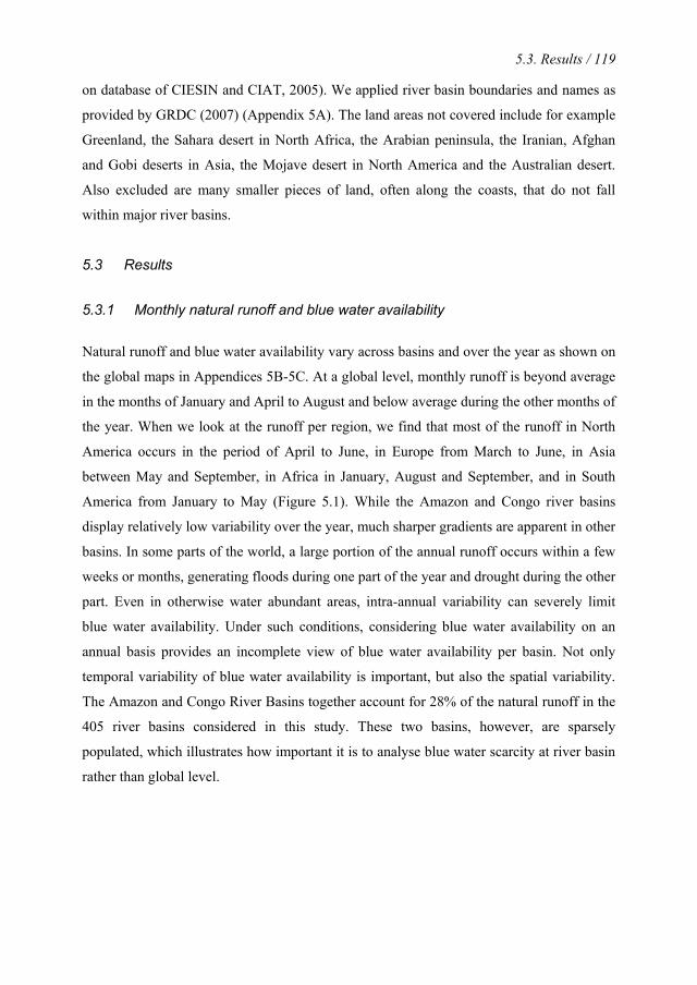
5.3. Results / 119
on database of CIESIN and CIAT, 2005). We applied river basin boundaries and names as
provided by GRDC (2007) (Appendix 5A). The land areas not covered include for example
Greenland, the Sahara desert in North Africa, the Arabian peninsula, the Iranian, Afghan
and Gobi deserts in Asia, the Mojave desert in North America and the Australian desert.
Also excluded are many smaller pieces of land, often along the coasts, that do not fall
within major river basins.
5.3 Results
5.3.1 Monthly natural runoff and blue water availability
Natural runoff and blue water availability vary across basins and over the year as shown on
the global maps in Appendices 5B-5C. At a global level, monthly runoff is beyond average
in the months of January and April to August and below average during the other months of
the year. When we look at the runoff per region, we find that most of the runoff in North
America occurs in the period of April to June, in Europe from March to June, in Asia
between May and September, in Africa in January, August and September, and in South
America from January to May (Figure 5.1). While the Amazon and Congo river basins
display relatively low variability over the year, much sharper gradients are apparent in other
basins. In some parts of the world, a large portion of the annual runoff occurs within a few
weeks or months, generating floods during one part of the year and drought during the other
part. Even in otherwise water abundant areas, intra-annual variability can severely limit
blue water availability. Under such conditions, considering blue water availability on an
annual basis provides an incomplete view of blue water availability per basin. Not only
temporal variability of blue water availability is important, but also the spatial variability.
The Amazon and Congo River Basins together account for 28% of the natural runoff in the
405 river basins considered in this study. These two basins, however, are sparsely
populated, which illustrates how important it is to analyse blue water scarcity at river basin
rather than global level.

120 / Chapter 5. Global blue water scarcity
5.3.2 Monthly blue water footprint
The current study has taken the blue water footprint (consumptive use of ground or surface
water) as a measure of freshwater use instead of water withdrawal as used in all earlier
water scarcity studies. Agriculture accounts for 92% of the global blue water footprint; the
remainder is equally shared between industrial production and domestic water supply
(Mekonnen and Hoekstra, 2011b). However, this share varies across river basins and within
the year. While the blue water footprint in agriculture varies from month to month
depending on the timing and intensity of irrigation, the domestic water supply and
industrial production were assumed to remain constant throughout the year. Therefore, for
particular months in certain basins one hundred per cent of the blue water footprint can be
attributed to industry and domestic water supply. The intra-annual variability of the total
blue water footprint for the major river basins is mapped in Appendix 5D. The values on
the maps are shown in mm per month and can thus directly be compared. A large blue
water footprint throughout the year is observed for the Indus and Ganges river basins,
because irrigation occurs here throughout the year. A large blue water footprint during part
of the year is estimated for basins such as the Tigris-Euphrates, Huang He (Yellow River),
Murray, Guadiana, Colorado (Pacific Ocean) and Krishna. When we consider Europe and
North America as a whole, we see a clear peak in the blue water footprint in the months
May to September (around the northern summer). In Australia, we see a blue water
footprint peak in the months October to March (around the southern summer). One cannot
find such profound patterns if one consider the blue water footprint throughout the year in
South America, Africa or Asia, because these continents are more heterogeneous (Figure
5.2).
5.3.3 Monthly blue water scarcity per river basin
The blue water scarcity for each of the twelve months of the year for the major river basins
in the world is presented in global maps in Figures 5.3a-5.3b. In each month that a river
basin is coloured in some shade of green, the monthly blue water scarcity is low (smaller
than 100%). The blue water footprint does not exceed blue water availability, which means
that environmental flow requirements are not violated. River runoff in that month is
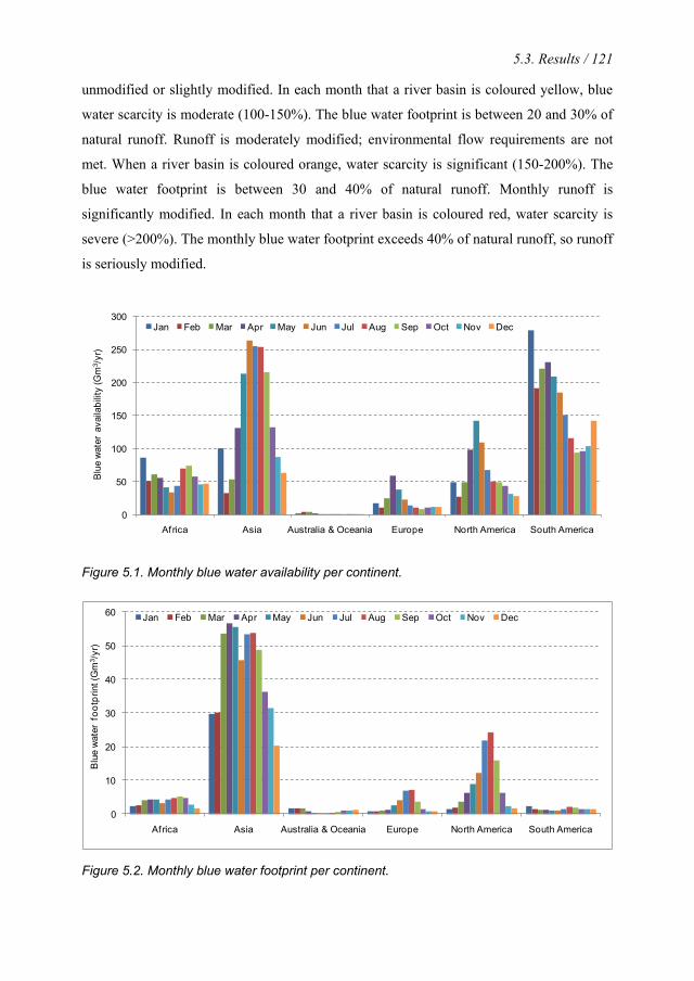
5.3. Results / 121
unmodified or slightly modified. In each month that a river basin is coloured yellow, blue
water scarcity is moderate (100-150%). The blue water footprint is between 20 and 30% of
natural runoff. Runoff is moderately modified; environmental flow requirements are not
met. When a river basin is coloured orange, water scarcity is significant (150-200%). The
blue water footprint is between 30 and 40% of natural runoff. Monthly runoff is
significantly modified. In each month that a river basin is coloured red, water scarcity is
severe (>200%). The monthly blue water footprint exceeds 40% of natural runoff, so runoff
is seriously modified.
0
50
100
150
200
250
300
Africa Asia Australia & Oceania Europe North America South America
Blu
e w
ater
ava
ilabi
lity
(Gm
3 /yr
)
Jan Feb Mar Apr May Jun Jul Aug Sep Oct Nov Dec
Figure 5.1. Monthly blue water availability per continent.
0
10
20
30
40
50
60
Africa Asia Australia & Oceania Europe North America South America
Blu
e w
ater
foo
tprin
t (G
m3 /
yr)
Jan Feb Mar Apr May Jun Jul Aug Sep Oct Nov Dec
Figure 5.2. Monthly blue water footprint per continent.

122 / Chapter 5. Global blue water scarcity
Figure 5.3a. Monthly blue water scarcity in the world’s major river basins (January-June). Period: 1996-2005.
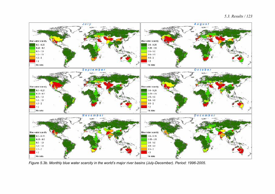
5.3. Results / 123
Figure 5.3b. Monthly blue water scarcity in the world’s major river basins (July-December). Period: 1996-2005.
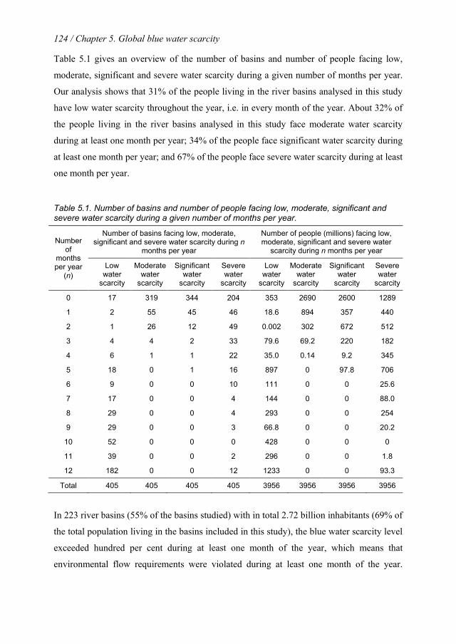
124 / Chapter 5. Global blue water scarcity
Table 5.1 gives an overview of the number of basins and number of people facing low,
moderate, significant and severe water scarcity during a given number of months per year.
Our analysis shows that 31% of the people living in the river basins analysed in this study
have low water scarcity throughout the year, i.e. in every month of the year. About 32% of
the people living in the river basins analysed in this study face moderate water scarcity
during at least one month per year; 34% of the people face significant water scarcity during
at least one month per year; and 67% of the people face severe water scarcity during at least
one month per year.
Table 5.1. Number of basins and number of people facing low, moderate, significant and severe water scarcity during a given number of months per year.
Number of
months per year
(n)
Number of basins facing low, moderate, significant and severe water scarcity during n
months per year
Number of people (millions) facing low, moderate, significant and severe water
scarcity during n months per year
Low water
scarcity
Moderate water
scarcity
Significant water
scarcity
Severe water
scarcity
Low water
scarcity
Moderate water
scarcity
Significant water
scarcity
Severe water
scarcity
0 17 319 344 204 353 2690 2600 1289
1 2 55 45 46 18.6 894 357 440
2 1 26 12 49 0.002 302 672 512
3 4 4 2 33 79.6 69.2 220 182
4 6 1 1 22 35.0 0.14 9.2 345
5 18 0 1 16 897 0 97.8 706
6 9 0 0 10 111 0 0 25.6
7 17 0 0 4 144 0 0 88.0
8 29 0 0 4 293 0 0 254
9 29 0 0 3 66.8 0 0 20.2
10 52 0 0 0 428 0 0 0
11 39 0 0 2 296 0 0 1.8
12 182 0 0 12 1233 0 0 93.3
Total 405 405 405 405 3956 3956 3956 3956
In 223 river basins (55% of the basins studied) with in total 2.72 billion inhabitants (69% of
the total population living in the basins included in this study), the blue water scarcity level
exceeded hundred per cent during at least one month of the year, which means that
environmental flow requirements were violated during at least one month of the year.
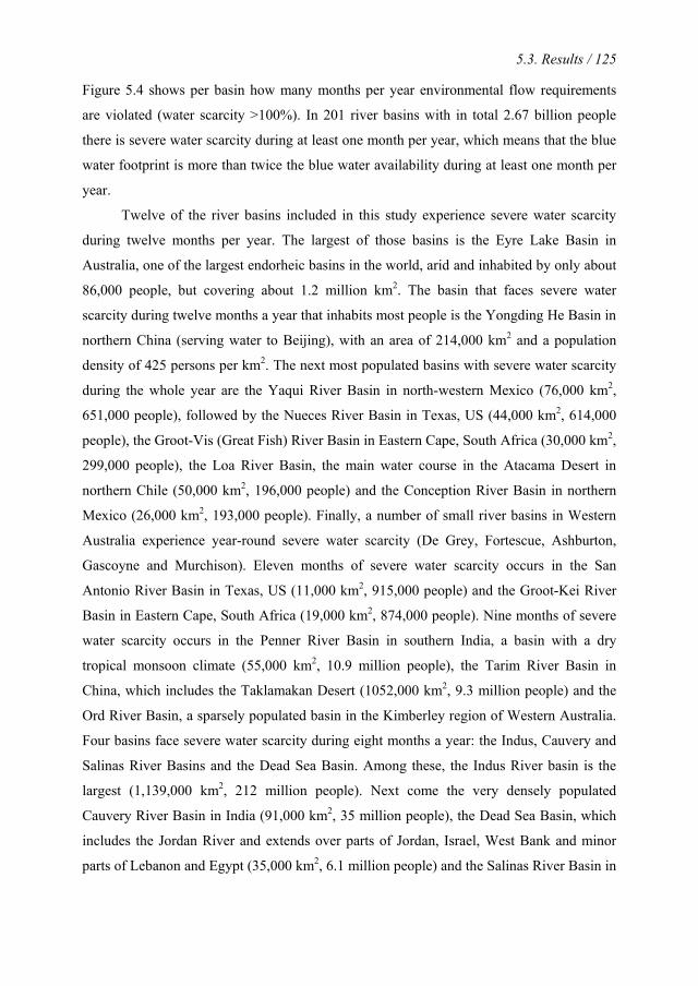
5.3. Results / 125
Figure 5.4 shows per basin how many months per year environmental flow requirements
are violated (water scarcity >100%). In 201 river basins with in total 2.67 billion people
there is severe water scarcity during at least one month per year, which means that the blue
water footprint is more than twice the blue water availability during at least one month per
year.
Twelve of the river basins included in this study experience severe water scarcity
during twelve months per year. The largest of those basins is the Eyre Lake Basin in
Australia, one of the largest endorheic basins in the world, arid and inhabited by only about
86,000 people, but covering about 1.2 million km2. The basin that faces severe water
scarcity during twelve months a year that inhabits most people is the Yongding He Basin in
northern China (serving water to Beijing), with an area of 214,000 km2 and a population
density of 425 persons per km2. The next most populated basins with severe water scarcity
during the whole year are the Yaqui River Basin in north-western Mexico (76,000 km2,
651,000 people), followed by the Nueces River Basin in Texas, US (44,000 km2, 614,000
people), the Groot-Vis (Great Fish) River Basin in Eastern Cape, South Africa (30,000 km2,
299,000 people), the Loa River Basin, the main water course in the Atacama Desert in
northern Chile (50,000 km2, 196,000 people) and the Conception River Basin in northern
Mexico (26,000 km2, 193,000 people). Finally, a number of small river basins in Western
Australia experience year-round severe water scarcity (De Grey, Fortescue, Ashburton,
Gascoyne and Murchison). Eleven months of severe water scarcity occurs in the San
Antonio River Basin in Texas, US (11,000 km2, 915,000 people) and the Groot-Kei River
Basin in Eastern Cape, South Africa (19,000 km2, 874,000 people). Nine months of severe
water scarcity occurs in the Penner River Basin in southern India, a basin with a dry
tropical monsoon climate (55,000 km2, 10.9 million people), the Tarim River Basin in
China, which includes the Taklamakan Desert (1052,000 km2, 9.3 million people) and the
Ord River Basin, a sparsely populated basin in the Kimberley region of Western Australia.
Four basins face severe water scarcity during eight months a year: the Indus, Cauvery and
Salinas River Basins and the Dead Sea Basin. Among these, the Indus River basin is the
largest (1,139,000 km2, 212 million people). Next come the very densely populated
Cauvery River Basin in India (91,000 km2, 35 million people), the Dead Sea Basin, which
includes the Jordan River and extends over parts of Jordan, Israel, West Bank and minor
parts of Lebanon and Egypt (35,000 km2, 6.1 million people) and the Salinas River Basin in
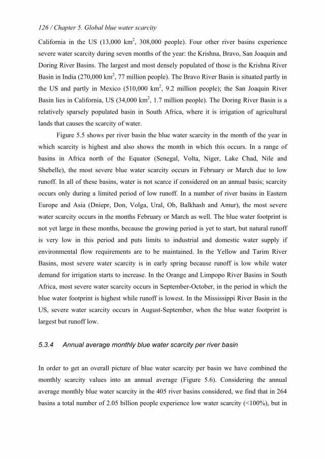
126 / Chapter 5. Global blue water scarcity
California in the US (13,000 km2, 308,000 people). Four other river basins experience
severe water scarcity during seven months of the year: the Krishna, Bravo, San Joaquin and
Doring River Basins. The largest and most densely populated of those is the Krishna River
Basin in India (270,000 km2, 77 million people). The Bravo River Basin is situated partly in
the US and partly in Mexico (510,000 km2, 9.2 million people); the San Joaquin River
Basin lies in California, US (34,000 km2, 1.7 million people). The Doring River Basin is a
relatively sparsely populated basin in South Africa, where it is irrigation of agricultural
lands that causes the scarcity of water.
Figure 5.5 shows per river basin the blue water scarcity in the month of the year in
which scarcity is highest and also shows the month in which this occurs. In a range of
basins in Africa north of the Equator (Senegal, Volta, Niger, Lake Chad, Nile and
Shebelle), the most severe blue water scarcity occurs in February or March due to low
runoff. In all of these basins, water is not scarce if considered on an annual basis; scarcity
occurs only during a limited period of low runoff. In a number of river basins in Eastern
Europe and Asia (Dniepr, Don, Volga, Ural, Ob, Balkhash and Amur), the most severe
water scarcity occurs in the months February or March as well. The blue water footprint is
not yet large in these months, because the growing period is yet to start, but natural runoff
is very low in this period and puts limits to industrial and domestic water supply if
environmental flow requirements are to be maintained. In the Yellow and Tarim River
Basins, most severe water scarcity is in early spring because runoff is low while water
demand for irrigation starts to increase. In the Orange and Limpopo River Basins in South
Africa, most severe water scarcity occurs in September-October, in the period in which the
blue water footprint is highest while runoff is lowest. In the Mississippi River Basin in the
US, severe water scarcity occurs in August-September, when the blue water footprint is
largest but runoff low.
5.3.4 Annual average monthly blue water scarcity per river basin
In order to get an overall picture of blue water scarcity per basin we have combined the
monthly scarcity values into an annual average (Figure 5.6). Considering the annual
average monthly blue water scarcity in the 405 river basins considered, we find that in 264
basins a total number of 2.05 billion people experience low water scarcity (<100%), but in
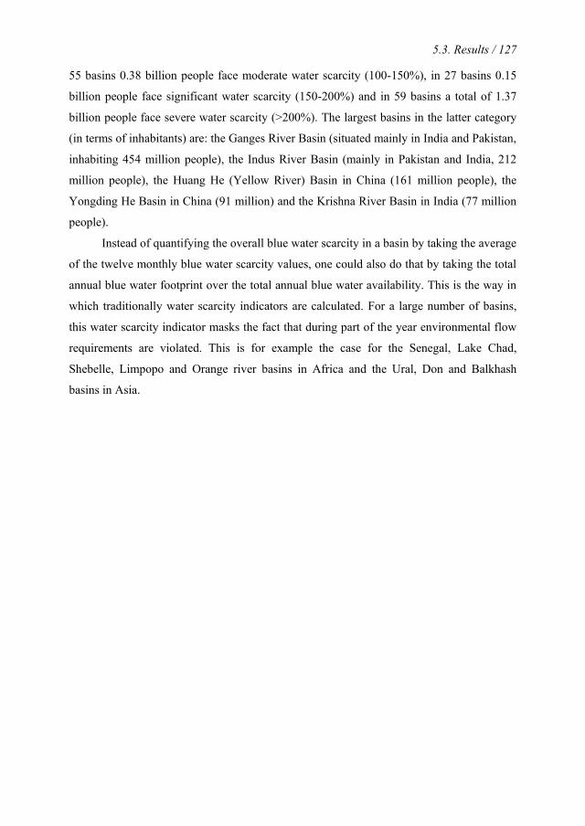
5.3. Results / 127
55 basins 0.38 billion people face moderate water scarcity (100-150%), in 27 basins 0.15
billion people face significant water scarcity (150-200%) and in 59 basins a total of 1.37
billion people face severe water scarcity (>200%). The largest basins in the latter category
(in terms of inhabitants) are: the Ganges River Basin (situated mainly in India and Pakistan,
inhabiting 454 million people), the Indus River Basin (mainly in Pakistan and India, 212
million people), the Huang He (Yellow River) Basin in China (161 million people), the
Yongding He Basin in China (91 million) and the Krishna River Basin in India (77 million
people).
Instead of quantifying the overall blue water scarcity in a basin by taking the average
of the twelve monthly blue water scarcity values, one could also do that by taking the total
annual blue water footprint over the total annual blue water availability. This is the way in
which traditionally water scarcity indicators are calculated. For a large number of basins,
this water scarcity indicator masks the fact that during part of the year environmental flow
requirements are violated. This is for example the case for the Senegal, Lake Chad,
Shebelle, Limpopo and Orange river basins in Africa and the Ural, Don and Balkhash
basins in Asia.
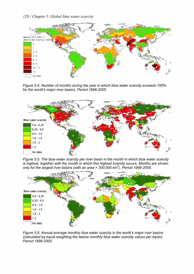
128 / Chapter 5. Global blue water scarcity
Figure 5.4. Number of months during the year in which blue water scarcity exceeds 100% for the world’s major river basins. Period 1996-2005.
Figure 5.5. The blue water scarcity per river basin in the month in which blue water scarcity is highest, together with the month in which this highest scarcity occurs. Months are shown only for the largest river basins (with an area > 300,000 km2). Period 1996-2005.
Figure 5.6. Annual average monthly blue water scarcity in the world’s major river basins (calculated by equal weighting the twelve monthly blue water scarcity values per basin). Period 1996-2005.
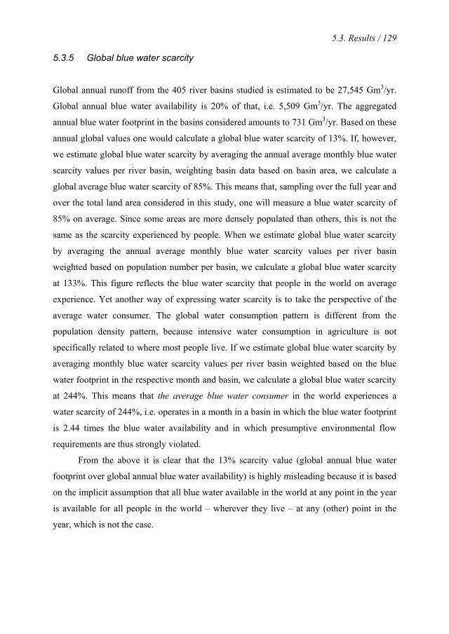
5.3. Results / 129
5.3.5 Global blue water scarcity
Global annual runoff from the 405 river basins studied is estimated to be 27,545 Gm3/yr.
Global annual blue water availability is 20% of that, i.e. 5,509 Gm3/yr. The aggregated
annual blue water footprint in the basins considered amounts to 731 Gm3/yr. Based on these
annual global values one would calculate a global blue water scarcity of 13%. If, however,
we estimate global blue water scarcity by averaging the annual average monthly blue water
scarcity values per river basin, weighting basin data based on basin area, we calculate a
global average blue water scarcity of 85%. This means that, sampling over the full year and
over the total land area considered in this study, one will measure a blue water scarcity of
85% on average. Since some areas are more densely populated than others, this is not the
same as the scarcity experienced by people. When we estimate global blue water scarcity
by averaging the annual average monthly blue water scarcity values per river basin
weighted based on population number per basin, we calculate a global blue water scarcity
at 133%. This figure reflects the blue water scarcity that people in the world on average
experience. Yet another way of expressing water scarcity is to take the perspective of the
average water consumer. The global water consumption pattern is different from the
population density pattern, because intensive water consumption in agriculture is not
specifically related to where most people live. If we estimate global blue water scarcity by
averaging monthly blue water scarcity values per river basin weighted based on the blue
water footprint in the respective month and basin, we calculate a global blue water scarcity
at 244%. This means that the average blue water consumer in the world experiences a
water scarcity of 244%, i.e. operates in a month in a basin in which the blue water footprint
is 2.44 times the blue water availability and in which presumptive environmental flow
requirements are thus strongly violated.
From the above it is clear that the 13% scarcity value (global annual blue water
footprint over global annual blue water availability) is highly misleading because it is based
on the implicit assumption that all blue water available in the world at any point in the year
is available for all people in the world – wherever they live – at any (other) point in the
year, which is not the case.
130 / Chapter 5. Global blue water scarcity
5.3.6 Blue water footprint versus blue water availability in selected river basins
Figures 5.7a-5.7c compare the blue water footprint with the blue water availability within
the course of the year for nine selected basins: the Tigris-Euphrates, Indus, Ganges, Huang
He, Tarim, Murray, Colorado, Guadiana and Limpopo. The blue water footprints refer to
the average over the period 1996-2005. The natural runoff and blue water availability refer
to climate averages. The figures show per river basin which parts of the blue water footprint
result in slight, moderate, significant and severe hydrological modification of the river. The
categories beyond slight modification mean that presumptive environmental flow
requirements are violated. Moderate hydrological modification occurs when blue water
footprint varies between 20 and 30 per cent of natural runoff; significant modification
happens when blue water footprint is 30-40 per cent of natural runoff; and severe
modification occurs when blue water footprint exceeds 40 per cent of natural runoff.
The Tigris-Euphrates River Basin extends over four countries: Turkey, Syria, Iraq
and Iran. Almost all of the runoff in the two rivers is generated in the highlands of the
northern and eastern parts of the basin in Turkey, Iraq and Iran. Precipitation in the basin is
largely confined to the winter months from October through April. The high waters occur
during the months of March through May as the snows melts on the highlands. The typical
low water season occurs from June to December. The basin faces severe water scarcity for
five months of the year (June-October). Most of the blue water footprint in the basin is due
to evaporation of irrigation water in agriculture, mostly for wheat, barley and cotton, which
together account for 52% of the total blue water footprint in the basin.
The Indus River Basin is a densely populated basin (186 persons/km2) facing severe
water scarcity almost three quarters of the year (September-April). The basin receives
around 70% of its precipitation during the months of June to October (Thenkabail et al.,
2005). The low-water period in the Indus River Basin is from November through February.
The high waters begin in June and continue through October as the snow and glaciers melt
from the Tibetan plateau. Over 93% of the blue water footprint related to crop production in
Pakistan occurs in the two major agricultural provinces of Punjab and Sindh which lie fully
(Punjab) and mostly (Sindh) in the basin. Irrigation of wheat, rice and cotton crops account
for 77% of the blue water footprint in the basin. Groundwater abstraction, mainly for
5.3. Results / 131
irrigation, goes beyond the natural recharge leading to depletion of the groundwater in the
basin (Wada et al., 2010).
The Ganges River Basin is one of the most densely populated basins in the world
(443 persons/km2). The basin is fed by two main headwaters in the Himalayas – the
Bhagirathi and Alaknanda – and many other tributaries that drain the Himalayas and the
Vindhya and Satpura ranges. The basin faces severe water scarcity for five months of the
year (January-May). Most of the blue water footprint in the basin is due to evaporation of
irrigation water in agriculture, mostly for wheat, rice and sugar cane. These three crops
together are responsible for 85% of the total blue water footprint in the basin.
Overexploitation of the aquifers for irrigation is leading to depletion of the groundwater in
the basin (Wada et al., 2010).
The Huang He (Yellow River) Basin in China faces severe water scarcity for four
months of the year (February-May). The low-water period in the Huang He River Basin is
from December through March. The river originates in the Bayankela Mountains of the
Tibetan Plateau. The high waters begin in April and continue through October. Most of the
blue water footprint in the basin is due to irrigation water use in agriculture, mostly for
wheat, maize and rice, which together account for 79% of the blue water footprint in the
basin. The dry conditions during part of the year coupled with the large water footprint
related to agricultural and industrial production and domestic water supply is leading to a
great pressure on the water resources of the basin. The Tarim River Basin faces severe water scarcity during three quarters of the year
(February-October). The low-water period in the Tarim Basin is from October through
April. The spring and summer high waters begin in May and continue through September
as the snows melts on the Tian Shan and Kunlun Shan mountains. Most of the blue water
footprint in the basin is due to evaporation of irrigation water in agriculture, mostly for
wheat, rice and maize. These three crops are responsible for 78% of the blue water footprint
in the Tarim River Basin.
The Murray River Basin, often called the Murray-Darling River Basin because of the
importance of the Darling River that joins the Murray River at Wentworth, is a very
important basin for agriculture in Australia. About 78% of the blue water footprint related
to crop production in Australia is in the Murray River Basin. Most of the blue water
footprint in the basin is due to evaporation of irrigation water in agriculture, mostly for

132 / Chapter 5. Global blue water scarcity
fodder crops, cotton and rice, which together constitute 77% of the blue water footprint
within the basin. The basin faces severe water scarcity for half of the year (November-
April).
The Colorado River Basin draining into the Pacific Ocean is a basin in the South-
western US (with a minor fraction in North-western Mexico). About 75% of the runoff in
the basin occurs during the months of April through July. During five months of year
(August-November and February) the basin faces severe water scarcity. Most of the blue
water footprint in the basin is due to evaporation of irrigation water in agriculture, mostly
for fodder crops and cotton, which make 73% of the blue water footprint in the Colorado
Basin. The Colorado River is considered the life line of the South-western US providing
water to millions of people both within and outside the basin, for irrigated land and
hydroelectricity generation (Pontius, 1997). Colorado River water is diverted for use both
in and outside of the basin. Annually, more than one third of the river’s supply is diverted
from the basin, including diversions to cities such as Denver, Colorado Springs, Salt Lake
City, Albuquerque, Los Angeles, and San Diego (Pontius, 1997). Due to its
overexploitation, little or no freshwater is discharged to the sea in dry years (Postel, 1998).
The Guadiana River Basin is shared by Spain and Portugal but mainly lies in South-
Eastern Spain. The basin faces severe water scarcity during half of the year (June-
November). The high-water period in the Guadiana Basin is from February through April.
Irrigation of maize, grapes and other perennial crops (mainly olives) account for the largest
share of the blue water footprint in the basin (55%). Overexploitation of the aquifer for
irrigation purposes is a major problem (Wada et al., 2010), occurring mainly in the upper
basin (Aldaya and Llamas, 2008).
The Limpopo River Basin faces severe water scarcity during five months of the year
(July-November). The low-water period in the Limpopo Basin is from May through
December. Most of the blue water footprint in the basin is due to evaporation of irrigation
water in agriculture, mostly for fodder crops, cotton and sugar cane, which together account
for 52% of the total blue water footprint in the basin.
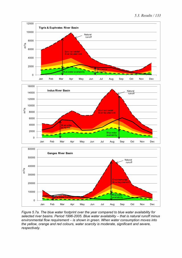
5.3. Results / 133
0
2000
4000
6000
8000
10000
12000
Jan Feb Mar Apr May Jun Jul Aug Sep Oct Nov Dec
m3 /
sTigris & Euphrates River Basin
Environmentalflow requirement
Naturalrunoff
Blue water availabilityBlue water footprint
0
2000
4000
6000
8000
10000
12000
14000
16000
Jan Feb Mar Apr May Jun Jul Aug Sep Oct Nov Dec
m3 /
s
Indus River Basin
Environmentalflow requirement
Naturalrunoff
Blue water availability
Blue water footprint
0
10000
20000
30000
40000
50000
60000
Jan Feb Mar Apr May Jun Jul Aug Sep Oct Nov Dec
m3 /
s
Ganges River Basin
Environmentalflow requirement
Naturalrunoff
Blue water availabilityBlue water footprint
Figure 5.7a. The blue water footprint over the year compared to blue water availability for selected river basins. Period 1996-2005. Blue water availability – that is natural runoff minus environmental flow requirement – is shown in green. When water consumption moves into the yellow, orange and red colours, water scarcity is moderate, significant and severe, respectively.

134 / Chapter 5. Global blue water scarcity
0
500
1000
1500
2000
2500
3000
3500
4000
4500
Jan Feb Mar Apr May Jun Jul Aug Sep Oct Nov Dec
m3 /
sHuang He (Yellow River) Basin
Environmentalflow requirement
Naturalrunoff
Blue water availability
Blue water footprint
0
200
400
600
800
1000
1200
1400
Jan Feb Mar Apr May Jun Jul Aug Sep Oct Nov Dec
m3 /
s
Tarim River Basin
Environmentalflow requirement
Naturalrunoff
Blue water availability
Blue water footprint
0
200
400
600
800
1000
1200
1400
Jan Feb Mar Apr May Jun Jul Aug Sep Oct Nov Dec
m3 /
s
Murray River Basin
Environmentalflow requirement
Naturalrunoff
Blue water availability
Blue water footprint
Figure 5.7b. The blue water footprint over the year compared to blue water availability for selected river basins. Period 1996-2005. Blue water availability – that is natural runoff minus environmental flow requirement – is shown in green. When water consumption moves into the yellow, orange and red colours, water scarcity is moderate, significant and severe, respectively.
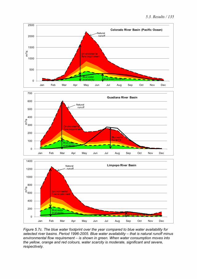
5.3. Results / 135
0
500
1000
1500
2000
2500
Jan Feb Mar Apr May Jun Jul Aug Sep Oct Nov Dec
m3 /
sColorado River Basin (Pacific Ocean)
Environmentalflow requirement
Naturalrunoff
Blue water availability Blue water footprint
0
100
200
300
400
500
600
700
Jan Feb Mar Apr May Jun Jul Aug Sep Oct Nov Dec
m3 /
s
Guadiana River Basin
Environmentalflow requirement
Naturalrunoff
Blue water availability
Blue water footprint
0
200
400
600
800
1000
1200
1400
Jan Feb Mar Apr May Jun Jul Aug Sep Oct Nov Dec
m3 /
s
Limpopo River Basin
Environmentalflow requirement
Naturalrunoff
Blue water availability
Blue water footprint
Figure 5.7c. The blue water footprint over the year compared to blue water availability for selected river basins. Period 1996-2005. Blue water availability – that is natural runoff minus environmental flow requirement – is shown in green. When water consumption moves into the yellow, orange and red colours, water scarcity is moderate, significant and severe, respectively.

136 / Chapter 5. Global blue water scarcity
5.4 Discussion and conclusion
The blue water scarcity estimates presented include uncertainties that reflect the
uncertainties in input data used and the assumptions that were made. The data on actual
runoff used are model-based estimates calibrated against long-term runoff measurements
(Fekete et al., 2002); the model outcomes include an error of 5% at the scale of large river
basins or beyond for smaller river basins. The runoff measurements against which the
model is calibrated include uncertainties as well; discharge measurements have an accuracy
on the order of ±10-20 per cent (Fekete et al., 2002). Estimates used for the blue water
footprints can easily contain an uncertainty of ±20% (Hoff et al., 2010; Mekonnen and
Hoekstra, 2010a,d); uncertainties for relatively small river basins are generally bigger than
for large river basins. An important assumption in the study is the presumptive standard on
environmental flow requirements based on Richter et al. (2011). Obviously, different
estimates of environmental flow requirements will affect the estimates of blue water
availability and thus scarcity.
In order to estimate natural runoff in each river basin, we have added the estimated
blue water footprint (from Mekonnen and Hoekstra, 2011b) to the estimated actual runoff
(from Fekete et al., 2002). In doing so, we overestimate natural runoff in those months in
which the blue water footprint (partially) originates from depleting the total water stock in
the basin rather than from runoff depletion. At the same time we underestimate the natural
runoff in the months in which water is being stored for later consumption. Further, as a
result of our approach we overestimate natural runoff in those months and basins in which
the blue water footprint (partially) originates from fossil (non-renewable) groundwater,
because that part should not be added to actual runoff to get natural runoff. However, data
on consumption of renewable versus fossil groundwater are hard to obtain at a global scale.
Given the uncertainties and the sensitivity of the outcomes of this study to the
assumptions made, the quantitative results presented in this study should be taken with
caution. However, the spatial and temporal water scarcity patterns and the order of
magnitudes of the results presented in this paper give a good indication of when and where
blue water scarcity is relatively low or high.
The calculated blue water scarcity values per river basin and month are conservative
estimates of actual scarcity for two reasons. First, by evaluating water scarcity at the level

5.4. Discussion and Conclusion / 137
of whole river basins, we do not capture spatial variations within the basins, so that the blue
water footprint may match blue water availability at the basin level while it does not at sub-
catchment level. Second, we consider an average year regarding both blue water
availability and footprint, while in many basins inter-annual variations can be substantial,
aggravating the scarcity problem in the dryer years.
The water scarcity values presented refer to the period 1996-2005. Continued growth
of the water footprint due to growing populations, changing food patterns (for instance in
the direction of more meat) and increasing demand for biomass for bio-energy combined
with the effects of climate change, are likely to result in growing blue water scarcity in the
future (Vörösmarty et al., 2000).
This study has quantified freshwater scarcity only in terms of blue water. For a
complete picture of the extent of freshwater scarcity one should also consider the use and
availability of green water and water pollution (Savenije, 2000; Rijsberman, 2006;
Rockstrom et al., 2009; Hoekstra et al., 2011). Therefore, future research should focus on
the development of a complete picture of water scarcity, including green water scarcity and
water pollution levels over time.
The current study provides the first global assessment of blue water scarcity in a
spatially and temporally explicit way. Water scarcity analysis at a monthly time step
provides insight into the real degree of water scarcity that is not revealed in existing annual
water scarcity indicators like those employed by for example Vörösmarty et al. (2000),
Alcamo and Henrichs (2002), Smakthin et al. (2004) and Oki and Kanae (2006). Ignoring
temporal variability in estimating blue water scarcity obscures the fact that scarcity occurs
in certain periods of the year and not in others. A similar problem occurs if one would
compare the global blue water footprint with global blue water availability. In this case one
obscures the fact that scarcity happens in certain basins, generally where most people live,
and not equally throughout the world.
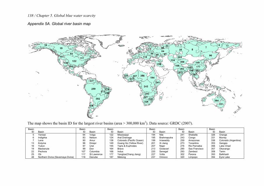
138 / Chapter 5. Global blue water scarcity
Appendix 5A. Global river basin map
The map shows the basin ID for the largest river basins (area > 300,000 km2). Data source: GRDC (2007). Basin
ID Basin Basin
ID Basin Basin
ID Basin Basin
ID Basin Basin
ID Basin Basin
ID Basin 5 Yenisei 64 Volga 122 Mississippi 194 Nile 241 Shebelle 326 Orange 6 Indigirka 83 Nelson 124 Aral Drainage 195 Brahmaputra 243 Congo 331 Murray 7 Lena 90 Amur 138 Colorado (Pacific Ocean) 199 Irrawaddy 259 Amazonas 336 Colorado (Argentina)
13 Kolyma 96 Dniepr 149 Huang He (Yellow River) 201 Xi Jiang 273 Tocantins 353 Ganges 16 Yukon 97 Ural 155 Tigris & Euphrates 207 Niger 276 Rio Parnaiba 356 Lake Chad 19 Mackenzie 99 Don 164 Bravo 213 Godavari 290 Sao Francisco 357 Okavango 22 Pechora 107 Columbia 168 Indus 220 Senegal 293 Zambezi 358 Tarim 25 Ob 117 St.Lawrence 177 Yangtze(Chang Jiang) 227 Volta 302 Parana 393 Balkhash 48 Northern Dvina (Severnaya Dvina) 118 Danube 187 Mekong 237 Orinoco 320 Limpopo 394 Eyre Lake
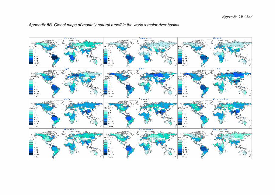
Appendix 5B / 139
Appendix 5B. Global maps of monthly natural runoff in the world’s major river basins
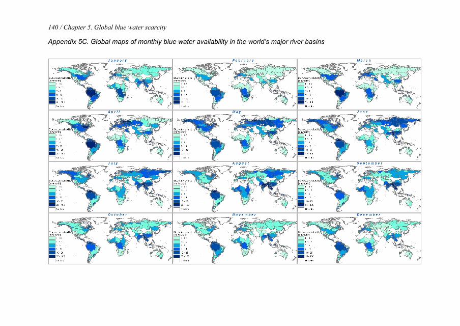
140 / Chapter 5. Global blue water scarcity
Appendix 5C. Global maps of monthly blue water availability in the world’s major river basins

Appendix 5D / 141
Appendix 5D. Global maps of the monthly blue water footprint in the world’s major river basins. Period 1996-2005.


6. A global and high-resolution assessment of the green, blue and grey water footprint of wheat5
Abstract
The aim of this study is to estimate the green, blue and grey water footprint of wheat in a
spatially-explicit way, both from a production and consumption perspective. The
assessment is global and improves upon earlier research by taking a high-resolution
approach, estimating the water footprint of the crop at a 5 by 5 arc minute grid. We have
used a grid-based dynamic water balance model to calculate crop water use over time, with
a time step of one day. The model takes into account the daily soil water balance and
climatic conditions for each grid cell. In addition, the water pollution associated with the
use of nitrogen fertilizer in wheat production is estimated for each grid cell. We have used
the water footprint and virtual water flow assessment framework as in the guideline of the
Water Footprint Network.
The global wheat production in the period 1996-2005 required about 1088 billion
cubic meters of water per year. The major portion of this water (70%) comes from green
water, about 19% comes from blue water, and the remaining 11% is grey water. The global
average water footprint of wheat per ton of crop was 1830 m3/ton. About 18% of the water
footprint related to the production of wheat is meant not for domestic consumption but for
export. About 55% of the virtual water export comes from the USA, Canada and Australia
alone. For the period 1996-2005, the global average water saving from international trade
in wheat products was 65 Gm3/yr.
A relatively large total blue water footprint as a result of wheat production is
observed in the Ganges and Indus river basins, which are known for their water stress
problems. The two basins alone account for about 47% of the blue water footprint related to
global wheat production. About 93% of the water footprint of wheat consumption in Japan
lies in other countries, particularly the USA, Australia and Canada. In Italy, with an average
wheat consumption of 150 kg/yr per person, more than two times the word average, about
5 Based on Mekonnen and Hoekstra (2010a,b)
144 / Chapter 6. A global assessment of water footprint of wheat
44% of the total water footprint related to this wheat consumption lies outside Italy. The
major part of this external water footprint of Italy lies in France and the USA.
6.1 Introduction
Fresh water is a renewable but finite resource. Both freshwater availability and quality vary
enormously in time and space. Growing populations coupled with continued socio-
economic developments put pressure on the globe’s scarce water resources. In many parts
of the world, there are signs that water consumption and pollution exceed a sustainable
level. The reported incidents of groundwater depletion, rivers running dry and worsening
pollution levels form an indication of the growing water scarcity (Gleick, 1993; Postel,
2000; WWAP, 2009). Molden (2007) argues that to meet the acute freshwater challenges
facing humankind over the coming fifty years requires substantial reduction of water use in
agriculture.
The concept of ‘water footprint’ introduced by Hoekstra (2003) and subsequently
elaborated by Hoekstra and Chapagain (2008) provides a framework to analyse the link
between human consumption and the appropriation of the globe’s freshwater. The water
footprint of a product is defined as the total volume of freshwater that is used to produce
the product (Hoekstra et al., 2009). The blue water footprint refers to the volume of surface
and groundwater consumed (evaporated) as a result of the production of a good; the green
water footprint refers to the rainwater consumed. The grey water footprint of a product
refers to the volume of freshwater that is required to assimilate the load of pollutants based
on existing ambient water quality standards. The water footprint of national consumption is
defined as the total amount of freshwater that is used to produce the goods consumed by the
inhabitants of the nation. The water footprint of national consumption always has two
components: the internal and the external footprint. The latter refers to the appropriation of
water resources in other nations for the production of goods and services that are imported
into and consumed within the nation considered. Externalising the water footprint reduces
the pressure on domestic water resources, but increases the pressure on the water resources
in other countries. Virtual water transfer in the form of international trade in agricultural
goods is increasingly recognized as a mechanism to save domestic water resources and
achieve national water security (Allan, 2003; Hoekstra, 2003; De Fraiture et al., 2004; Liu
6.1. Introduction / 145
et al., 2007; Oki and Kanae, 2004; Chapagain et al., 2006a; Yang et al., 2006; Hoekstra and
Chapagain, 2008). Virtual water import is an instrument that enables nations to save scarce
domestic water resources by importing water-intensive products and exporting
commodities that require less water. On the other hand, water-abundant countries can profit
by exporting water-intensive commodities.
In this paper, we focus on the water footprint of wheat, which is one of the most
widely cultivated cereal grains globally. It is grown on more land area than any other
commercial crop and is the second most produced cereal crop after maize and a little above
rice. It is believed to originate in Southwest Asia and the most likely site of its first
domestication is near Diyarbakir in Turkey (Dubcovsky and Dvorak, 2007). About 90 to 95
percent of the wheat produced is the common wheat or bread wheat followed by durum
wheat which accounts less than 5% of world wheat production (Pena, 2002; Ekboir, 2002).
Based on the growing period, wheat can be subdivided into spring and winter wheat. The
difference between spring and winter wheat is accounted for by taking specific crop
parameters, rooting depth and growing period.
A number of previous studies on global water use for wheat are already available.
Hoekstra and Hung (2002, 2005) were the first to make a global estimate of the water use in
wheat production. They analysed the period 1995-99 and looked at total evapotranspiration,
not distinguishing between green and blue water consumption. Hoekstra and Chapagain
(2007a, 2008) improved this first study in a number of respects and studied the period
1997-2001. Still, no distinction between green and blue water consumption was made. Liu
et al. (2007) made a global estimate of water consumption in wheat production for the
period 1998-2002 without making the green-blue water distinction, but for the first time
grid-based. Liu et al. (2009) and Liu and Yang (2010) present similar results, but now they
show the green-blue water distinction. Siebert and Döll (2008, 2010) have estimated the
global water consumption for wheat production for the same period as Liu et al. (2007,
2009), showing the green-blue water distinction and applying a grid-based approach as
well. Gerbens et al. (2009a) estimated the green and blue water footprint for wheat in the 25
largest producing countries. Aldaya et al. (2010b) have calculated the green and blue water
components for wheat in four major producing countries and also estimate international
virtual water flows related to wheat trade. Aldaya and Hoekstra (2010) made an assessment
146 / Chapter 6. A global assessment of water footprint of wheat
of the water footprint of wheat in different regions of Italy, for the first time specifying not
only the green and blue, but the grey water footprint as well.
The aim of this study is to estimate the green, blue and grey water footprint of wheat
in a spatially-explicit way, both from a production and consumption perspective. We
quantify the green, blue and grey water footprint of wheat production by using a grid-based
dynamic water balance model that takes into account local climate and soil conditions and
nitrogen fertilizer application rates and calculates the crop water requirements, actual crop
water use and yields and finally the green, blue and grey water footprint at grid level. The
model has been applied at a spatial resolution of 5 arc minutes by 5 arc minutes. The
model’s conceptual framework is based on the FAO CROPWAT approach (Doorenbos and
Pruitt, 1977; Doorenbos and Kassam, 1979; Allen et al., 1998). The water footprint of
wheat consumption per country is estimated by tracing the different sources of wheat
consumed in a country and considering the specific water footprints of wheat production in
the producing regions.
6.2 Method
In this study the global green, blue and grey water footprint of wheat production and
consumption and the international virtual water flows related to wheat trade were estimated
following the calculation framework of Hoekstra and Chapagain (2008) and Hoekstra et al.
(2009). The computations of crop evapotranspiration and yield, required for the estimation
of the green and blue water footprint in wheat production, have been done following the
method and assumptions provided by Allen et al. (1998) for the case of crop growth under
non-optimal conditions (Chapter 8). The grid-based dynamic water balance model
developed in this study for estimating the crop evapotranspiration and yield computes a
daily soil water balance and calculates crop water requirements, actual crop water use (both
green and blue) and actual yields. The model is applied at a global scale using a resolution
level of 5 by 5 arc minute grid size (about 10 km by 10 km around the Equator). The water
balance model is largely written in Python language and embedded in a computational
framework where input and output data are in grid-format. The input data available in grid-
format (like precipitation, reference evapotranspiration, soil, crop parameters) are converted
6.2. Method / 147
to text-format to feed the Python code. Output data from the Python code are converted
back to grid-format.
The actual crop evapotranspiration (ETa, mm/day) depends on climate parameters
(which determine potential evapotranspiration), crop characteristics and soil water
availability (Allen et al., 1998):
[ ] [ ] [ ] [ ]a c s oET t K t K t ET t= × × (20)
where Kc is the crop coefficient, Ks [t] a dimensionless transpiration reduction factor
dependent on available soil water and ETo[t] the reference evapotranspiration (mm/day).
The crop coefficient varies in time, as a function of the plant growth stage. During the
initial and mid-season stages of the crop development, Kc is a constant and equals Kc,ini and
Kc,mid respectively. During the crop development and late season stages, Kc varies linearly
and linear interpolation is applied for days within the development and late growing
seasons. The value of Ks is calculated on a daily basis as a function of the maximum and
actual available soil moisture in the root zone.
Following the approach as in the HBV model (Bergström, 1995; Lidén and Harlin,
2000) the amount of rainfall lost through runoff is computed as:
( ) [ ][ ]max
1[ ] [ ] [ ]
1S t
RO t P t I tS t
γ −
= + × − (21)
in which RO[t] is runoff on day t [mm]; P[t] precipitation on day t [mm]; I[t] the net
irrigation depth on day t that infiltrates the soil [mm]. The value of the parameter γ is
adopted from Siebert and Döll (2010) and was set to 3 for irrigated land and to 2 for rain-
fed areas.
The irrigation requirement is determined based on the root zone depletion. The
actual irrigation I[t] depends on the extent to which the irrigation requirement is met:
]t[IRα]t[I ×= (22)
148 / Chapter 6. A global assessment of water footprint of wheat
where α is the fraction of the irrigation requirement that is actually met. Following the
method as proposed in Hoekstra et al. (2009) and also applied by Siebert and Döll (2010),
we run two scenarios, one with α = 0 (no application of irrigation, i.e. rain-fed conditions)
and the other with α = 1 (full irrigation). In the second scenario we have assumed that the
amount of actual irrigation is sufficient to meet the irrigation requirement. In the case of
rain-fed wheat production, blue crop water use is zero and green crop water use (m3/ha) is
calculated by summing up the daily values of ETa (mm/day) over the length of the growing
period. In the case of irrigated wheat production, the green crop water use is assumed to be
equal to the green crop water use as was calculated for the rain-fed case. The blue crop
water use is then equal to the total ETa over the growing period as simulated under the case
α = 1 (full irrigation) minus the green crop water use.
The crop growth and yield are affected by the water stress. To account for the effect
of water stress, a linear relationship between yield and crop evapotranspiration was
proposed by Doorenbos and Kassam (1979):
−=
−
∑∑
][
][11
tCWR
tETK
YY a
ym
a (23)
where Ky is a yield response factor (water stress coefficient), Ya the actual harvested yield
[kg/ha], Ym the maximum yield [kg/ha], ETa the actual crop evapotranspiration in
mm/period and CWR the crop water requirement in mm/period (which is equal to Kc × ET0).
Ky values for individual periods and the complete growing period are given in Doorenbos
and Kassam (1979). The Ky values for the total growing period for winter wheat and spring
wheat are 1.0 and 1.15 respectively. The maximum yield value for a number of countries is
obtained from Ekboir (2002) and Pingali (1999). For countries with no such data the
regional average value is taken. The actual yields which are calculated per grid cell are
averaged over the nation and compared with the national average yield data (for the period
1996-2005) obtained from FAO (2010a). The calculated yield values are scaled to fit the
national average FAO yield data.
The green and blue water footprints (m3/ton) are calculated by dividing the green and
blue crop water use (m3/ha), respectively, by the actual crop yield (ton/ha). Both the total
6.2. Method / 149
green and the total blue water footprint in each grid cell are calculated as the weighted
average of the (green, respectively blue) water footprints under the two scenarios:
)0()1()1( =×−+=×= αβαβ WFWFWF (24)
where β refers to the fraction of wheat area in the grid cell that is irrigated.
The grey water footprint of wheat production is calculated by quantifying the volume of
water needed to assimilate the fertilisers that reach ground- or surface water. Nutrients
leaching or running off from agricultural fields are the main cause of non-point source
pollution of surface and subsurface water bodies. In this study we have quantified the grey
water footprint related to nitrogen use only. The grey component of the water footprint of
wheat (WFgy, m3/ton) is calculated by multiplying the leaching-runoff fraction (δ, %) by the
nitrogen application rate (AR, kg/ha) and dividing this by the difference between the
maximum acceptable concentration of nitrogen (cmax, kg/m3) and the natural concentration
of nitrogen in the receiving water body (cnat, kg/m3) and by the actual wheat yield (Ya,
ton/ha):
max
1gy
nat a
ARWFc c Yδ ×
= × − (25)
The average green, blue and grey water footprints of wheat in a whole nation or river basin
were estimated by taking the area-weighted average of the water footprint (m3/ton) over the
relevant grid cells.
The water footprints of wheat as harvested (unmilled wheat) have been used as a
basis to calculate the water footprints of derived wheat products (wheat flour, wheat groats
and meal, wheat starch and gluten) based on product and value fractions following the
method as in Hoekstra et al. (2009).
International virtual water flows (m3/yr) related to trade in wheat products were
calculated by multiplying the trade volumes (tons/yr) by their respective water footprint
(m3/ton). The global water saving (m3/yr) through international trade in wheat products is

150 / Chapter 6. A global assessment of water footprint of wheat
calculated by multiplying the volume of trade (ton/yr) between two countries by the
difference between the water footprint of the traded product in the importing country and
the water footprint of the product in the exporting country.
The water footprint of national wheat consumption can be distinguished into an
internal and external component. The internal water footprint is defined as the use of
domestic water resources to produce goods and services consumed by inhabitants of the
country. It is the water footprint related to production within the country minus the volume
of virtual water export to other countries insofar as related to export of domestically
produced products. The external water footprint is the part of the water footprint of national
consumption that falls outside the nation considered. It refers to the appropriation of water
resources in other nations for the production of goods and services that are imported into
and consumed within the nation considered
6.3 Data
Average monthly reference evapotranspiration data at 10 arc minute resolution were
obtained from FAO (2010d). The 10 minute data were converted to 5 arc minute resolution
by assigning the 10 minute data to each of the four 5 minute grid cells. Following the
CROPWAT approach, the monthly average data were converted to daily values by curve
fitting to the monthly average through polynomial interpolation.
Monthly values for precipitation, wet days and minimum and maximum temperature
with a spatial resolution of 30 arc minute were obtained from CRU-TS-2.1 (Mitchell and
Jones, 2005). The 30 arc minute data were assigned to each of the thirty-six 5 arc minute
grid cells contained in the 30 arc minute grid cell. Daily precipitation values were generated
from these monthly average values using the CRU-dGen daily weather generator model
(Schuol and Abbaspour, 2007).
Wheat growing areas on a 5 arc minute grid cell resolution were obtained from
Monfreda et al. (2008). For countries missing grid data in Monfreda et al. (2008) the
MICRA grid database as described in Portmann et al. (2010) was used to fill the gap. The
harvested wheat areas as available in grid format were aggregated to a national level and
scaled to fit national average wheat harvest areas for the period 1996-2005 obtained from
6.3. Data / 151
FAO (2010a). Grid data on irrigated wheat area per country were obtained from Portmann
et al. (2010).
Crop coefficients (Kc’s) for wheat were obtained from Chapagain and Hoekstra
(2004). Wheat planting dates and lengths of cropping seasons for most wheat producing
countries and regions were obtained from Sacks et al. (2010) and Portmann et al. (2010).
For some countries, values from Chapagain and Hoekstra (2004) were used. We have not
considered multi-cropping practices.
Grid based data on total available water capacity of the soil (TAWC) at a 5 arc
minute resolution were taken from ISRIC-WISE (Batjes, 2006). An average value of
TAWC of the five soil layers was used in the model.
Country-specific nitrogen fertilizer application rates for wheat have been based on
Heffer (2009), FAO (2006, 2010c) and IFA (2009). Globally, wheat accounts for about
17% of total fertilizer use and 19% of the total nitrogen fertilizer consumption. A number
of authors show that about 45-85% of the applied nitrogen fertilizer is recovered by the
plant (Addiscot, 1996, King et al., 2001, Ma et al., 2009, Noulas et al., 2004). On average,
about 16% of the applied nitrogen is presumed to be lost either by denitrification or
leaching (Addiscot, 1996). The reported value of nitrogen leaching varies between 2-13%
(Addiscot, 1996, Goulding et al., 2000, Riley et al., 2001, Webster et al., 1999). In this
study we have assumed that on average 10% of the applied nitrogen fertilizer is lost
through leaching or runoff, following Chapagain et al. (2006b). The recommended standard
value of nitrate in surface and groundwater by the World Health Organization and the
European Union is 50 mg nitrate (NO3) per litre and the standard recommended by US-
EPA is 10 mg per litre measured as nitrate-nitrogen (NO3-N). In this study we have used
the standard of 10 mg/litre of nitrate-nitrogen (NO3-N), following again Chapagain et al.
(2006b). Because of a lack of data, the natural nitrogen concentrations were assumed to be
zero.
Data on international trade in wheat products have been taken from the SITA
database (Statistics for International Trade Analysis) available from the International Trade
Centre (ITC, 2007). This database covers trade data over ten years (1996-2005) from 230
reporting countries disaggregated by product and partner countries. We have taken the
average for the period 1996-2005 in wheat products trade.
152 / Chapter 6. A global assessment of water footprint of wheat
6.4 The water footprint of wheat from the production perspective
The global water footprint of wheat production for the period 1996-2005 is 1088 Gm3/year
(70% green, 19% blue, and 11% grey). Data per country are shown in Table 6.1 for the
largest producers. The global green water footprint related to wheat production was 760
Gm3/yr. At a country level, large green water footprints can be found in the USA (112
Gm3/yr), China (83 Gm3/yr), Russia (91 Gm3/yr), Australia (44 Gm3/yr), and India (44
Gm3/yr). About 49% of the global green water footprint related to wheat production is in
these five countries. At sub-national level (state or province level), the largest green water
footprints can be found in Kansas in the USA (21 Gm3/yr), Saskatchewan in Canada (18
Gm3/yr), Western Australia (15 Gm3/yr), and North Dakota in the USA (15 Gm3/yr). The
global blue water footprint was estimated to be 204 Gm3/yr. The largest blue water
footprints were calculated for India (81 Gm3/yr), China (47 Gm3/yr), Pakistan (28 Gm3/yr),
Iran (11 Gm3/yr), Egypt (5.9 Gm3/yr) and the USA (5.5 Gm3/yr). These six countries
together account for 88% of the total blue water footprint related to wheat production. At
sub-national level, the largest blue water footprints can be found in Uttar Pradesh (24
Gm3/yr) and Madhya Pradesh (21 Gm3/yr) in the India and Punjab in Pakistan (20 Gm3/yr).
These three states in the two countries alone account about 32% of the global blue water
footprint related to wheat production. The grey water footprint related to the use of nitrogen
fertilizer in wheat cultivation was 124 Gm3/yr. The largest grey water footprint was
observed for China (32 Gm3/yr), India (20 Gm3/yr) the USA (14 Gm3/yr) and Pakistan (8
Gm3/yr).
The calculated global average water footprint per ton of wheat was 1830 m3/ton. The
results show a great variation, however, both within a country and among countries (Figure
6.1). Among the major wheat producers, the highest total water footprint per ton of wheat
was found for Morocco, Iran and Kazakhstan. On the other side of the spectrum, there are
countries like the UK and France with a wheat water footprint of around 560 - 600 m3/ton.
The global average blue water footprint per ton of wheat amounts to 343 m3/ton. For
a few countries, including Pakistan, India, Iran and Egypt, the blue water footprint is much
higher, up to 1478 m3/ton in Pakistan. In Pakistan, the blue water component in the total
water footprint is nearly 58%. The grey water footprint per ton of wheat is 208 m3/ton as a
global average, but in Poland it is 2.5 times higher than the global average.
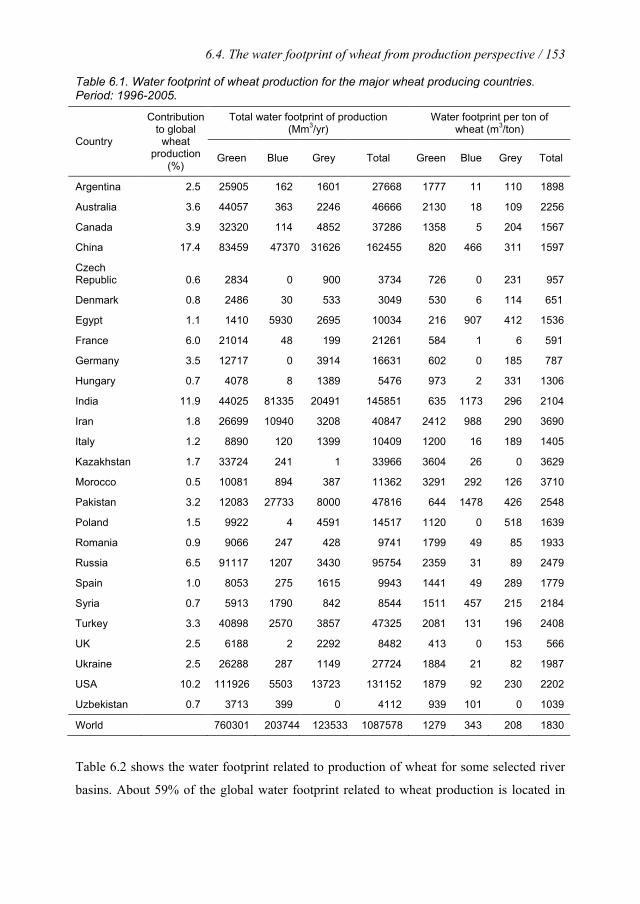
6.4. The water footprint of wheat from production perspective / 153
Table 6.1. Water footprint of wheat production for the major wheat producing countries. Period: 1996-2005.
Country
Contribution to global wheat
production (%)
Total water footprint of production (Mm3/yr)
Water footprint per ton of wheat (m3/ton)
Green Blue Grey Total Green Blue Grey Total
Argentina 2.5 25905 162 1601 27668 1777 11 110 1898
Australia 3.6 44057 363 2246 46666 2130 18 109 2256
Canada 3.9 32320 114 4852 37286 1358 5 204 1567
China 17.4 83459 47370 31626 162455 820 466 311 1597
Czech Republic 0.6 2834 0 900 3734 726 0 231 957
Denmark 0.8 2486 30 533 3049 530 6 114 651
Egypt 1.1 1410 5930 2695 10034 216 907 412 1536
France 6.0 21014 48 199 21261 584 1 6 591
Germany 3.5 12717 0 3914 16631 602 0 185 787
Hungary 0.7 4078 8 1389 5476 973 2 331 1306
India 11.9 44025 81335 20491 145851 635 1173 296 2104
Iran 1.8 26699 10940 3208 40847 2412 988 290 3690
Italy 1.2 8890 120 1399 10409 1200 16 189 1405
Kazakhstan 1.7 33724 241 1 33966 3604 26 0 3629
Morocco 0.5 10081 894 387 11362 3291 292 126 3710
Pakistan 3.2 12083 27733 8000 47816 644 1478 426 2548
Poland 1.5 9922 4 4591 14517 1120 0 518 1639
Romania 0.9 9066 247 428 9741 1799 49 85 1933
Russia 6.5 91117 1207 3430 95754 2359 31 89 2479
Spain 1.0 8053 275 1615 9943 1441 49 289 1779
Syria 0.7 5913 1790 842 8544 1511 457 215 2184
Turkey 3.3 40898 2570 3857 47325 2081 131 196 2408
UK 2.5 6188 2 2292 8482 413 0 153 566
Ukraine 2.5 26288 287 1149 27724 1884 21 82 1987
USA 10.2 111926 5503 13723 131152 1879 92 230 2202
Uzbekistan 0.7 3713 399 0 4112 939 101 0 1039
World 760301 203744 123533 1087578 1279 343 208 1830
Table 6.2 shows the water footprint related to production of wheat for some selected river
basins. About 59% of the global water footprint related to wheat production is located in

154 / Chapter 6. A global assessment of water footprint of wheat
this limited number of basins. Large blue water footprints can be found in the Ganges-
Brahmaputra-Meghna (53 Gm3/yr), Indus (42 Gm3/yr), Yellow (13 Gm3/yr), Tigris-
Euphrates (10 Gm3/yr), Amur (3.1 Gm3/yr) and Yangtze river basins (2.7 Gm3/yr). The
Ganges-Brahmaputra-Meghna and Indus river basins together account for about 47% of the
global blue and 21% of the global grey water footprint.
Table 6.2. The water footprint of wheat production for some selected river basins (1996-2005).
River basin Total water footprint of production
(Mm3/yr) Water footprint per ton of
wheat (m3/ton)
Green Blue Grey Total Green Blue Grey Total
Ganges-Brahmaputra-Meghna 30288 53009 12653 95950 665 1164 278 2107
Mississippi 79484 2339 9413 91236 1979 58 234 2271
Indus 22897 42145 13326 78368 604 1111 351 2066
Ob 51984 225 511 52721 2680 12 26 2718
Nelson-Saskatchewan 38486 118 5691 44294 1275 4 189 1468
Tigris-Euphrates 29219 10282 2670 42170 2893 1018 264 4175
Yellow 17012 13127 7592 37731 695 536 310 1541
Danube 27884 273 3579 31735 1298 13 167 1477
Volga 25078 272 955 26305 2315 25 88 2429
Don 24834 384 927 26144 2658 41 99 2799
Yangtze 17436 2700 4855 24991 1112 172 310 1594
Murray-Darling 20673 343 987 22003 2061 34 98 2193
La Plata 17127 73 1070 18271 2039 9 127 2175
Amur 8726 3136 2355 14216 985 354 266 1604
Dnieper 13219 68 813 14100 1732 9 107 1847
Columbia 7238 1877 1122 10236 1852 480 287 2620
Oral 9338 94 192 9624 2542 26 52 2620
World 760301 203744 123533 1087578 1279 343 208 1830
The global average water footprint of rain-fed wheat production is 1805 m3/ton, while in
irrigated wheat production it is 1868 m3/ton (Table 6.3). Obviously, the blue water footprint
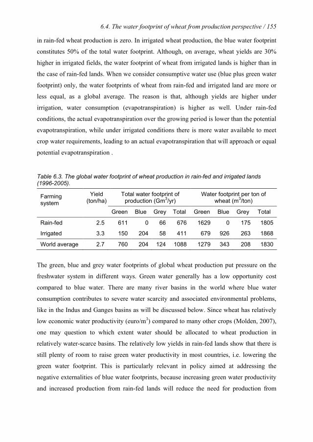
6.4. The water footprint of wheat from production perspective / 155
in rain-fed wheat production is zero. In irrigated wheat production, the blue water footprint
constitutes 50% of the total water footprint. Although, on average, wheat yields are 30%
higher in irrigated fields, the water footprint of wheat from irrigated lands is higher than in
the case of rain-fed lands. When we consider consumptive water use (blue plus green water
footprint) only, the water footprints of wheat from rain-fed and irrigated land are more or
less equal, as a global average. The reason is that, although yields are higher under
irrigation, water consumption (evapotranspiration) is higher as well. Under rain-fed
conditions, the actual evapotranspiration over the growing period is lower than the potential
evapotranspiration, while under irrigated conditions there is more water available to meet
crop water requirements, leading to an actual evapotranspiration that will approach or equal
potential evapotranspiration .
Table 6.3. The global water footprint of wheat production in rain-fed and irrigated lands (1996-2005).
Farming system
Yield (ton/ha)
Total water footprint of production (Gm3/yr)
Water footprint per ton of wheat (m3/ton)
Green Blue Grey Total Green Blue Grey Total
Rain-fed 2.5 611 0 66 676 1629 0 175 1805
Irrigated 3.3 150 204 58 411 679 926 263 1868
World average 2.7 760 204 124 1088 1279 343 208 1830
The green, blue and grey water footprints of global wheat production put pressure on the
freshwater system in different ways. Green water generally has a low opportunity cost
compared to blue water. There are many river basins in the world where blue water
consumption contributes to severe water scarcity and associated environmental problems,
like in the Indus and Ganges basins as will be discussed below. Since wheat has relatively
low economic water productivity (euro/m3) compared to many other crops (Molden, 2007),
one may question to which extent water should be allocated to wheat production in
relatively water-scarce basins. The relatively low yields in rain-fed lands show that there is
still plenty of room to raise green water productivity in most countries, i.e. lowering the
green water footprint. This is particularly relevant in policy aimed at addressing the
negative externalities of blue water footprints, because increasing green water productivity
and increased production from rain-fed lands will reduce the need for production from
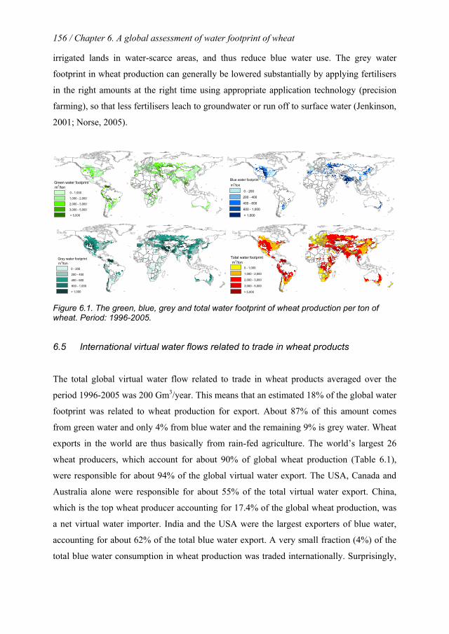
156 / Chapter 6. A global assessment of water footprint of wheat
irrigated lands in water-scarce areas, and thus reduce blue water use. The grey water
footprint in wheat production can generally be lowered substantially by applying fertilisers
in the right amounts at the right time using appropriate application technology (precision
farming), so that less fertilisers leach to groundwater or run off to surface water (Jenkinson,
2001; Norse, 2005).
Grey water footprintm3/ton
0 - 200
200 - 400
400 - 600
600 - 1,000
> 1,000
Total water footprintm3/ton
0 - 1,000
1,000 - 2,000
2,000 - 3,000
3,000 - 5,000
> 5,000
Green water footprintm3/ton
0 - 1,000
1,000 - 2,000
2,000 - 3,000
3,000 - 5,000
> 5,000
Blue water footprintm3/ton
0 - 200
200 - 400
400 - 600
600 - 1,000
> 1,000
Figure 6.1. The green, blue, grey and total water footprint of wheat production per ton of wheat. Period: 1996-2005.
6.5 International virtual water flows related to trade in wheat products
The total global virtual water flow related to trade in wheat products averaged over the
period 1996-2005 was 200 Gm3/year. This means that an estimated 18% of the global water
footprint was related to wheat production for export. About 87% of this amount comes
from green water and only 4% from blue water and the remaining 9% is grey water. Wheat
exports in the world are thus basically from rain-fed agriculture. The world’s largest 26
wheat producers, which account for about 90% of global wheat production (Table 6.1),
were responsible for about 94% of the global virtual water export. The USA, Canada and
Australia alone were responsible for about 55% of the total virtual water export. China,
which is the top wheat producer accounting for 17.4% of the global wheat production, was
a net virtual water importer. India and the USA were the largest exporters of blue water,
accounting for about 62% of the total blue water export. A very small fraction (4%) of the
total blue water consumption in wheat production was traded internationally. Surprisingly,

6.5. International virtual water flows / 157
some water-scarce regions in the world, relying on irrigation, show a net export of blue
water virtually embedded in wheat. Saudi Arabia had a net blue virtual water export of 21
Mm3/yr and Iraq exported a net volume of blue water of 6 Mm3/yr. The largest grey water
exporters were the USA, Canada, Australia and Germany. Data per country are shown in
Table 6.4 for the largest virtual water exporters and importers, respectively. The largest net
virtual water flows related to international wheat trade are shown in Figure 6.2.
Table 6.4. Gross virtual water export and import related to the international trade of wheat products in the period 1996-2005.
Largest virtual water exporters (Mm3/yr) Largest virtual water importers (Mm3/yr)
Green Blue Grey Total Green Blue Grey Total
USA 48603 2389 5959 56952 Brazil 11415 88 801 12304
Canada 24144 85 3625 27854 Japan 10393 320 1147 11860
Australia 24396 201 1244 25841 Italy 7345 174 760 8279
Argentina 15973 100 987 17060 Egypt 6838 274 633 7745
Kazakhstan 16490 118 0 16608 Korea, Rep 6511 398 685 7594
France 9347 21 89 9457 Indonesia 6512 364 577 7453
Russian Fed 7569 100 285 7954 Iran 6105 60 504 6670
Ukraine 4587 50 200 4837 Malaysia 5616 185 636 6437
Germany 3537 0 1090 4626 Algeria 5330 323 696 6350
India 1266 2338 589 4193 Mexico 5155 205 660 6020
Turkey 2208 139 208 2555 Russian Fed 5334 69 92 5495
UK 1189 0 441 1630 Philippines 3923 426 538 4887
Spain 1242 42 249 1534 Spain 4161 80 493 4734
Hungary 1035 2 352 1389 China 4087 98 453 4638
Others 13107 2202 2488 17797 Others 85967 4725 9131 99823
Global flow 174693 7789 17807 200289 Global flow 174693 7789 17807 200289
The global water saving associated with the international trade in wheat products adds up to
65 Gm3/yr (39% green, 48% blue, and 13% grey). Import of wheat and wheat products by
Algeria, Iran, Morocco and Venezuela from Canada, France, the USA and Australia
resulted in the largest global water savings. Figure 6.3 illustrates the concept of global
water saving through an example of the trade in durum wheat from France to Morocco.
158 / Chapter 6. A global assessment of water footprint of wheat
6.6 The water footprint of wheat from the consumption perspective
The global water footprint related to the consumption of wheat products was estimated at
1088 Gm3/yr, which is 177 m3/yr per person on average (70% green, 19% blue, and 11%
grey). About 82% of the total water footprint related to consumption was from domestic
production while the remaining 18% was external water footprint (Figure 6.4). In terms of
water footprint per capita, Kazakhstan has the largest water footprint, with 1156 m3/cap/yr,
followed by Australia and Iran with 1082 and 716 m3/cap/yr respectively. Data per country
are shown in Table 6.5 for the major wheat consuming countries and in Figure 6.5 all
countries of the world. When the water footprint of wheat consumption per capita is
relatively high in a country, this can be explained by either one or a combination of two
factors: (i) the wheat consumption in the country is relatively high; (ii) the wheat consumed
has a high water footprint per kg of wheat. As one can see in Table 6.5, in the case of
Kazakhstan and Iran, both factors play a role. In the case of Australia, the relatively high
water footprint related to wheat consumption can be mostly explained by the high wheat
consumption per capita alone. Germany has a large wheat consumption per capita – more
than twice the world average – so that one would expect that the associated water footprint
would be high as well, but this is not the case because, on average, the wheat consumed in
Germany has a low water footprint per kg (43% of the global average).
The countries with the largest external water footprint related to wheat consumption
were Brazil, Japan, Egypt, Italy, the Republic of Korea and Iran. Together, these countries
account for about 28% of the total external water footprint. Japan’s water footprint related
to wheat consumption lies outside the country for about 93%. In Italy, with an average
wheat consumption of 150 kg/yr per person, more than two times the word average, this
was about 44%. Most African, South-East Asian, Caribbean and Central American
countries strongly rely on external water resources for their wheat consumption as shown in
Figure 6.6.

6.6. The water footprint of wheat from the consumption perspective / 159
Figure 6.2. National virtual water balances and net virtual water flows related to trade in wheat products in the period 1996-2005. Only the largest net flows (> 2 Gm3/yr) are shown.
France
Water footprint , WFe= 591 m3/ton
MoroccoWater footprint , WFi= 5710 m3/ton
Wheat tradeT = 905,882 ton/yr
Global water saving∆Sg =T(WFi-WFe) = 905,882(5710-591) = 3.17 Gm3/yr
National water saving∆Sn = WFi x T = 5710 x 905,882 = 3.77 Gm3/yr
National water loss∆Sn = WFe x T = 591 x 905,882 = 0.6 Gm3/yr
Figure 6.3. Global water saving through the trade in durum wheat from France to Morocco. Period: 1996-2005.
Green water footprint54.6%
Blue water footprint18.1%
Grey water footprint9.8%
Green water footprint15.3%
Blue water footprint0.7%
Grey water footprint1.5%
Internal water footprint82%
External water footprint18%
Total water footprint = 1088 Gm3/yrPer capita water footprint =177 m3/cap/yr
Figure 6.4. Global water footprint related the consumption of wheat products. Period: 1996-2005.
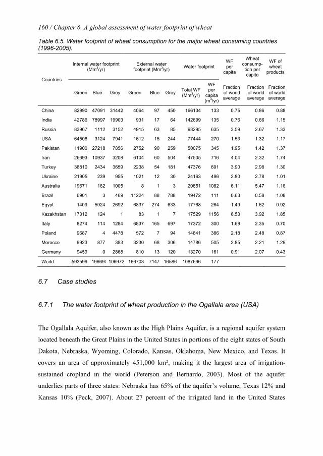
160 / Chapter 6. A global assessment of water footprint of wheat
Table 6.5. Water footprint of wheat consumption for the major wheat consuming countries (1996-2005).
Countries
Internal water footprint (Mm3/yr)
External water footprint (Mm3/yr) Water footprint
WF per
capita
Wheat consump-tion per capita
WF of wheat
products
Green Blue Grey Green Blue Grey Total WF (Mm3/yr)
WF per
capita (m3/yr)
Fraction of world average
Fraction of world average
Fraction of world average
China 82990 47091 31442 4064 97 450 166134 133 0.75 0.86 0.88
India 42786 78997 19903 931 17 64 142699 135 0.76 0.66 1.15
Russia 83967 1112 3152 4915 63 85 93295 635 3.59 2.67 1.33
USA 64508 3124 7941 1612 15 244 77444 270 1.53 1.32 1.17
Pakistan 11900 27218 7856 2752 90 259 50075 345 1.95 1.42 1.37
Iran 26693 10937 3208 6104 60 504 47505 716 4.04 2.32 1.74
Turkey 38810 2434 3659 2238 54 181 47376 691 3.90 2.98 1.30
Ukraine 21905 239 955 1021 12 30 24163 496 2.80 2.78 1.01
Australia 19671 162 1005 8 1 3 20851 1082 6.11 5.47 1.16
Brazil 6901 3 469 11224 88 788 19472 111 0.63 0.58 1.08
Egypt 1409 5924 2692 6837 274 633 17768 264 1.49 1.62 0.92
Kazakhstan 17312 124 1 83 1 7 17529 1156 6.53 3.92 1.85
Italy 8274 114 1284 6837 165 697 17372 300 1.69 2.35 0.70
Poland 9687 4 4478 572 7 94 14841 386 2.18 2.48 0.87
Morocco 9923 877 383 3230 68 306 14786 505 2.85 2.21 1.29
Germany 9459 0 2868 810 13 120 13270 161 0.91 2.07 0.43
World 593599 196690 106972 166703 7147 16586 1087696 177
6.7 Case studies
6.7.1 The water footprint of wheat production in the Ogallala area (USA)
The Ogallala Aquifer, also known as the High Plains Aquifer, is a regional aquifer system
located beneath the Great Plains in the United States in portions of the eight states of South
Dakota, Nebraska, Wyoming, Colorado, Kansas, Oklahoma, New Mexico, and Texas. It
covers an area of approximately 451,000 km², making it the largest area of irrigation-
sustained cropland in the world (Peterson and Bernardo, 2003). Most of the aquifer
underlies parts of three states: Nebraska has 65% of the aquifer’s volume, Texas 12% and
Kansas 10% (Peck, 2007). About 27 percent of the irrigated land in the United States
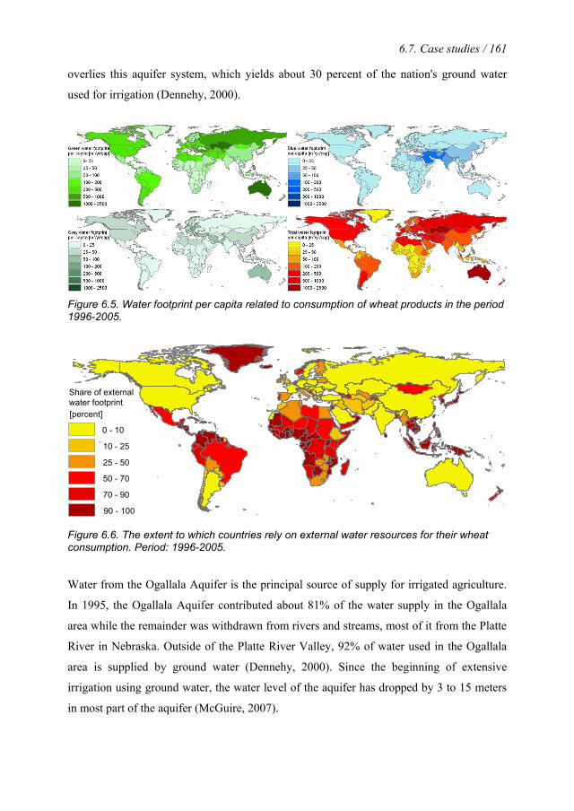
6.7. Case studies / 161
overlies this aquifer system, which yields about 30 percent of the nation's ground water
used for irrigation (Dennehy, 2000).
Figure 6.5. Water footprint per capita related to consumption of wheat products in the period 1996-2005.
Share of external water footprint [percent]
0 - 10
10 - 25
25 - 50
50 - 70
70 - 90
90 - 100
Figure 6.6. The extent to which countries rely on external water resources for their wheat consumption. Period: 1996-2005.
Water from the Ogallala Aquifer is the principal source of supply for irrigated agriculture.
In 1995, the Ogallala Aquifer contributed about 81% of the water supply in the Ogallala
area while the remainder was withdrawn from rivers and streams, most of it from the Platte
River in Nebraska. Outside of the Platte River Valley, 92% of water used in the Ogallala
area is supplied by ground water (Dennehy, 2000). Since the beginning of extensive
irrigation using ground water, the water level of the aquifer has dropped by 3 to 15 meters
in most part of the aquifer (McGuire, 2007).
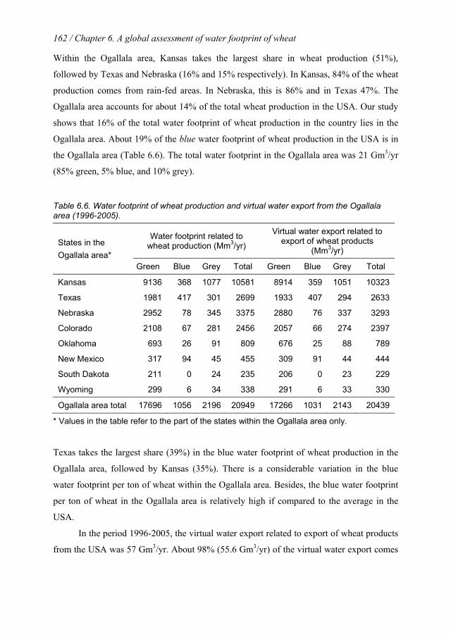
162 / Chapter 6. A global assessment of water footprint of wheat
Within the Ogallala area, Kansas takes the largest share in wheat production (51%),
followed by Texas and Nebraska (16% and 15% respectively). In Kansas, 84% of the wheat
production comes from rain-fed areas. In Nebraska, this is 86% and in Texas 47%. The
Ogallala area accounts for about 14% of the total wheat production in the USA. Our study
shows that 16% of the total water footprint of wheat production in the country lies in the
Ogallala area. About 19% of the blue water footprint of wheat production in the USA is in
the Ogallala area (Table 6.6). The total water footprint in the Ogallala area was 21 Gm3/yr
(85% green, 5% blue, and 10% grey).
Table 6.6. Water footprint of wheat production and virtual water export from the Ogallala area (1996-2005).
States in the Ogallala area*
Water footprint related to wheat production (Mm3/yr)
Virtual water export related to export of wheat products
(Mm3/yr)
Green Blue Grey Total Green Blue Grey Total
Kansas 9136 368 1077 10581 8914 359 1051 10323
Texas 1981 417 301 2699 1933 407 294 2633
Nebraska 2952 78 345 3375 2880 76 337 3293
Colorado 2108 67 281 2456 2057 66 274 2397
Oklahoma 693 26 91 809 676 25 88 789
New Mexico 317 94 45 455 309 91 44 444
South Dakota 211 0 24 235 206 0 23 229
Wyoming 299 6 34 338 291 6 33 330
Ogallala area total 17696 1056 2196 20949 17266 1031 2143 20439
* Values in the table refer to the part of the states within the Ogallala area only.
Texas takes the largest share (39%) in the blue water footprint of wheat production in the
Ogallala area, followed by Kansas (35%). There is a considerable variation in the blue
water footprint per ton of wheat within the Ogallala area. Besides, the blue water footprint
per ton of wheat in the Ogallala area is relatively high if compared to the average in the
USA.
In the period 1996-2005, the virtual water export related to export of wheat products
from the USA was 57 Gm3/yr. About 98% (55.6 Gm3/yr) of the virtual water export comes
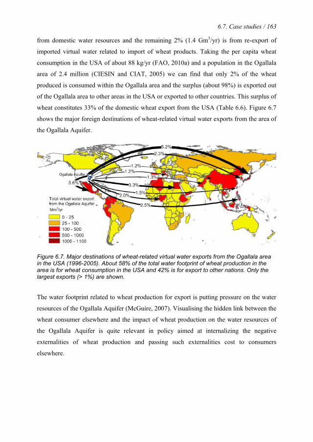
6.7. Case studies / 163
from domestic water resources and the remaining 2% (1.4 Gm3/yr) is from re-export of
imported virtual water related to import of wheat products. Taking the per capita wheat
consumption in the USA of about 88 kg/yr (FAO, 2010a) and a population in the Ogallala
area of 2.4 million (CIESIN and CIAT, 2005) we can find that only 2% of the wheat
produced is consumed within the Ogallala area and the surplus (about 98%) is exported out
of the Ogallala area to other areas in the USA or exported to other countries. This surplus of
wheat constitutes 33% of the domestic wheat export from the USA (Table 6.6). Figure 6.7
shows the major foreign destinations of wheat-related virtual water exports from the area of
the Ogallala Aquifer.
Figure 6.7. Major destinations of wheat-related virtual water exports from the Ogallala area in the USA (1996-2005). About 58% of the total water footprint of wheat production in the area is for wheat consumption in the USA and 42% is for export to other nations. Only the largest exports (> 1%) are shown.
The water footprint related to wheat production for export is putting pressure on the water
resources of the Ogallala Aquifer (McGuire, 2007). Visualising the hidden link between the
wheat consumer elsewhere and the impact of wheat production on the water resources of
the Ogallala Aquifer is quite relevant in policy aimed at internalizing the negative
externalities of wheat production and passing such externalities cost to consumers
elsewhere.
164 / Chapter 6. A global assessment of water footprint of wheat
6.7.2 The water footprint of wheat production in the Ganges and Indus river
basins
The Ganges river basin, which is part of the composite Ganges-Brahmaputra-Meghna river
basin, is one of most densely populated river basins in the world. It covers about 1 million
km2 (Gleick, 1993). The Indus river basin, which extends over four countries (China, India,
Pakistan and Afghanistan), is also a highly populated river basin. The area of the Indus
basin is a bit smaller than the Ganges basin but covers nearly 1 million km2 as well (Gleick,
1993).
The two river basins together account for about 90 percent of the wheat production
in India and Pakistan in the period 1996-2005. Almost all wheat production (98%) in
Pakistan comes from the Indus river basin. About 89% of India’s wheat is produced in the
Ganges (62%) and the Indus basin (27%). About 87% of the total water footprint related to
wheat production in India and Pakistan lies in these two river basins. The total water
footprint of wheat production in the Indian part of the Ganges basin is 92 Gm3/yr (32%
green, 54% blue, 14% grey). The total water footprint of wheat production in the Pakistani
part of the Indus basin is 48 Gm3/yr (25% green, 58% blue, 17% grey).
In the period 1996-2005, India and Pakistan together had a virtual water export
related to wheat export of 5.1 Gm3/yr (29% green water, 56% blue, 15% grey), which is a
small fraction (3%) of the total water footprint of wheat production in these two countries.
About 55% of this total virtual water export comes from the Ganges basin and 45% from
the Indus basin. The blue water export to other countries from the Ganges and Indus river
basins was 1304 Mm3/yr and 1077 Mm3/yr respectively.
Based on the water withdrawal-to-availability ratio, which is an indicator of water
stress (Alcamo et al., 2003a; Alcamo et al., 2007; Cosgrove and Rijsberman, 2000), most
parts of Pakistan and India are highly water stressed (Alcamo et al., 2003b). Both the
Ganges and Indus river basins are under severe water stress, in particular the Indus river
basin. About 97% of the water footprint related to wheat production in the two basins is for
domestic consumption within the two countries. Since the two basins are the wheat baskets
of the two countries, there are substantial virtual water transfers from the Ganges and Indus
basins to other areas within India and Pakistan. By looking at the virtual flows both within
the country and to other countries, it is possible to link the impacts of wheat consumption in
6.7. Case studies / 165
other places to the water stress in the Ganges and Indus basins. For the case of India,
Kampman et al. (2008) have shown that the states which lie within the Indus and Ganges
river basins, such as Punjab, Uttar Pradesh and Haryana are the largest inter-state virtual
water exporters within India. The highly subsidized irrigation water in these regions has led
to an intensive exploitation of the available water resources in these areas compared to
other, more water-abundant regions of India. In order to provide incentives for water
protection, negative externalities such as water overexploitation and pollution, and also
scarcity rents should be included in the price of the crop. Both basins have a relatively high
water productivity, which is shown by a smaller water footprint per ton of wheat, compared
to other wheat producing areas in the two countries (Figure 6.8). Since wheat is a low-value
crop, one may question whether water allocation to wheat production for export in states
such as Punjab, Uttar Pradesh and Haryana is worth the cost. A major destination of wheat
exports from India’s parts of the Indus and Ganges basins is East India, to states like Bihar.
Major foreign destinations of India’s virtual water export related to export of wheat
products are Bangladesh (22%), Indonesia (11%), Philippines (10%) and Yemen (10%).
Pakistan’s export mainly goes to Afghanistan (56%) and Kenya (11%).
6.7.3 The external water footprint of wheat consumption in Italy and Japan
In the previous two sections we have looked into the water footprint of wheat production in
specific areas of the world and analysed how this water footprints could be linked to
consumers elsewhere. In this section we will do the reverse: we will consider the wheat
consumers in two selected countries – Italy and Japan – and trace where their water
footprint lies.
Italy’s water footprint related to the consumption of wheat products for the period
1996-2005 was 17.4 Gm3/yr. More than half (56%) of Italy’s water footprint is pressing on
domestic water systems. The rest of the water footprint of Italian wheat consumption lies in
other countries, mainly the USA (20%), France (19%), Canada (11%) and Russia (10%).
The water footprint of Italy’s wheat consumers in the USA lies in different regions of that
country, among others in the Ogallala area as earlier shown in Figure 6.7. Italy also imports
virtual water from the water-scarce countries of the Middle East, such as Syria (58 Mm3/yr)
and Iraq (36 Mm3/yr).

166 / Chapter 6. A global assessment of water footprint of wheat
Figure 6.8. The total and blue water footprint related to wheat production in India and Pakistan, both expressed as a total (Mm3/yr) and per ton of wheat (m3/ton). Period: 1996-2005.
About 93% of the water footprint of wheat consumption in Japan lies in other countries,
mainly in the USA (59%), Australia (22%) and Canada (19%). About 87% of Japan’s
external water footprint is from green water. Japan’s wheat-related water footprint in the
USA partly presses on the water resources of the Ogallala area as shown in Figure 6.7. The
water footprint in Australia largely lies in Southern Australia where most of the wheat is
produced and water scarcity is high.
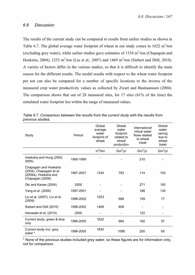
6.8. Discussion / 167
6.8 Discussion
The results of the current study can be compared to results from earlier studies as shown in
Table 6.7. The global average water footprint of wheat in our study comes to 1622 m3/ton
(excluding grey water), while earlier studies gave estimates of 1334 m3/ton (Chapagain and
Hoekstra, 2004), 1253 m3/ton (Liu et al., 2007) and 1469 m3/ton (Siebert and Döll, 2010).
A variety of factors differ in the various studies, so that it is difficult to identify the main
reason for the different results. The model results with respect to the wheat water footprint
per ton can also be compared for a number of specific locations to the inverse of the
measured crop water productivity values as collected by Zwart and Bastiaanssen (2004).
The comparison shows that out of 28 measured sites, for 17 sites (61% of the time) the
simulated water footprint lies within the range of measured values.
Table 6.7. Comparison between the results from the current study with the results from previous studies.
Study Period
Global average
water footprint of
wheat
Global water
footprint related to
wheat production
International virtual water flows related
to wheat trade
Global water saving due to wheat trade
m3/ton Gm3/yr Gm3/yr Gm3/yr
Hoekstra and Hung (2002, 2005) 1995-1999 - - 210 -
Chapagain and Hoekstra (2004), Chapagain et al. (2006a), Hoekstra and Chapagain (2008)
1997-2001 1334 793 114 103
Oki and Kanae (2004) 2000 - - 271 193
Yang et al. (2006) 1997-2001 - - 188 130
Liu et al. (2007), Liu et al. (2009) 1998-2002 1253 688 159 77
Siebert and Döll (2010) 1998-2002 1469 858 - -
Hanasaki et al. (2010) 2000 - - 122 -
Current study, green & blue only 1996-2005 1622 964 182 57
Current study incl. grey water * 1996-2005 1830 1088 200 65
* None of the previous studies included grey water, so these figures are for information only, not for comparison.
168 / Chapter 6. A global assessment of water footprint of wheat
The model results with respect to the total global water footprint of wheat production can
be compared to three previous global wheat studies. The study by Chapagain and Hoekstra
(2004) did not take a grid-based approach and also did not make the green-blue distinction,
unlike the current study and the studies by Siebert and Döll (2010) and Liu et al. (2009),
therefore we will compare here only with the latter two. When we compare the computed
green and blue water footprints to the computation by Siebert and Döll (2010), we find that
their estimate of the total water footprint of global wheat production is 11% lower, which is
completely due to their lower estimate of the green water footprint component. The
estimate of the total water footprint by Liu et al. (2009) is 29% lower than our estimate,
again due to the difference in the estimate of the green component. The relatively low value
presented by Liu et al. (2009) is not a surprise given the fact that their estimate is based on
the GEPIC model, which has been shown to give low estimates of evapotranspiration
compared to other models (Hoff et al., 2010). Our estimate of the total green water footprint
in global wheat production is 760 Gm3/yr (period 1996-2005), whereas Siebert and Döll
(2010) give an estimation of 650 Gm3/yr (period 1998-2002) and Liu et al. (2009) 540
Gm3/yr (1998-2002). Our estimate of the total blue water footprint in global wheat
production is 204 Gm3/yr, whereas Siebert and Döll (2010) give an estimation of 208
Gm3/yr and Liu et al. (2009) 150 Gm3/yr.
Liu et al. (2009) use another water balance model than applied in the current study.
As a basis, they use the EPIC model (Williams et al., 1989), whereas we apply the model of
Allen et al. (1998). Although both models compute the same variables, EPIC has been
developed as a crop growth model, whereas the model of Allen et al. (1998) has been
developed as a water balance model, which makes that the two models have a different
structure and different parameters. One of the differences is the runoff model applied,
which affects the soil water balance and thus soil water availability and finally the green
water footprint. Besides, Liu et al. (2009) estimate water footprints (m3/ton) based on
computed yields, whereas we use computed yields, but scale them according to FAO
statistics. Siebert and Döll (2010) basically apply the same modelling approach as in the
current study. Both studies have the same spatial resolution, carry out a soil water balance
with a daily time step, use the same CRU TS-2.1 climate data source to generate the daily
precipitation and use the same crop, soil and irrigation maps. Although there are many
similarities, the studies differ in some respects. For estimating daily reference

6.8. Discussion / 169
evapotranspiration data, Siebert and Döll (2010) applied the cubic splin method to generate
daily climate data from the monthly data as provided in the available database. In contrast,
we have used long-term monthly average reference evapotranspiration global spatial data
obtained from FAO (2010d) and converted these data to daily values by polynomial
interpolation. Further, Siebert and Döll (2010) have considered multi-cropping based on a
number of assumptions and generated their own cropping calendar based on climatic data,
while in our study we have neglected multi-cropping and adopted cropping calendars as
provided in literature at country level. Siebert and Döll (2010) compute local yields and
scale them later on, like in the current study, but scaling is done in different manner.
Finally, in our study we include the grey water footprint and study international virtual
water flows, which is not done by Siebert and Döll (2010).
It is difficult to make a conclusion about the accuracy or reliability of our estimates
vice versa the quality of the data presented in the other two modelling studies cited. All
studies depend on a large set of assumptions with respect to modelling structure, parameter
values, datasets used and period considered. For the time being, it is probably best to
conclude that the divergence in outcomes is a reflection of the uncertainties involved. It
implies that all estimates – both from the current and the previous studies – should be
interpreted with care. Assuming that the different study periods are comparable, the three
studies together give an estimation of the total water footprint of wheat production of about
830 Gm3/yr ± 17%. This uncertainty range is probably still a conservative estimate, because
it is based on the central estimates of three different modelling studies only. Furthermore,
locally, differences and uncertainty ranges can be larger.
The green water footprint estimate is sensitive to a variety of assumptions, including:
(a) the daily rain pattern (b) the modelling of runoff, (c) the rooting depth, (d) the soil type,
which determines the soil water holding capacity, (e) the planting and harvesting dates and
thus the length of the growing period, (f) the moisture content in the soil at the moment of
planting, (g) the modelling of yield. The blue water footprint estimate depends on the same
assumptions, plus it depends on data on actual irrigation. In a global study, given the
limitations in global databases, it seems very difficult in this stage to reduce the
uncertainties. Higher resolution maps of all input parameters and variables, based on either
local measurements or remote sensing (Romaguera et al., 2010) may finally help to reduce
the uncertainties in a global assessment like this one. In local studies, it will generally be

170 / Chapter 6. A global assessment of water footprint of wheat
less time-consuming to find better estimates for the various parameters and data involved
and better be able to validate the model used for the specific local conditions, so that
uncertainties can be reduced more easily.
The estimation of the grey water footprint in this study is based on a simplified
approach, assuming a certain leaching-runoff fraction and a maximum acceptable
concentration of nitrogen in the receiving water body. This approach gives a rough
estimate; it leaves out local factors that influence the precise leaching rates, such as rainfall
intensity, soil property and the amount of the already mineralized nitrogen in the upper soil
layer. A possible improvement in estimating the amount of nitrogen lost through leaching
would be to use more advanced models such as De Willigen (2000) regression model. This
model has been used by a number of studies including FAO (Roy et al. 2003), Smaling et
al. (2008) in the Brazilian soybean agriculture study, Haileslassie et al. (2007) in the
nutrient flows and balance study in the central highland of Ethiopia, and Lesschen et al.
(2007) in the soil nutrient balance study in Burkina Faso. Most recently, Liu et al. (2010)
have shown the application of the model in a high-resolution assessment of global nitrogen
flows in cropland.
Estimating water footprints of crops at national level and estimating international
virtual water flows based on those national estimates – as done in all previous global water
footprint studies until date – hides the existing variation at sub-national level in climatic
conditions, water resources availability and crop yields. Therefore, the present study is an
attempt to improve water footprint accounting through implementing the calculations at a
grid basis, which takes into account the existing heterogeneity at grid level. Such approach
has the advantage of being able to pinpoint precisely in space where the water footprint of
wheat consumption is located. We have combined the water footprint assessment
framework as provided in Hoekstra and Chapagain (2008) and Hoekstra et al. (2009) with a
grid-based approach to estimating crop evapotranspiration as applied by for example Liu et
al. (2009) and Siebert and Döll (2010).
6.8. Discussion / 171
6.9 Conclusion
The major findings of the current study are that: (i) the green water footprint related to
global wheat production is about four times larger than the blue water footprint, (ii) a large
amount of global water saving occurs as a result of international trade in wheat products –
without trade the global wheat-related water footprint would be 6% higher than under
current conditions, (iii) the high share of blue water (48%) in the global water saving
indicates that the water footprint of wheat in the largest virtual water export regions is
dominated by green water while virtual water import regions depend more strongly on blue
water for wheat production. The study agrees with earlier studies in the importance of green
water in global wheat production and the relevance of virtual water trade in global water
savings. It is observed that the costs of water consumption and pollution are not yet
properly factored into the price of traded wheat, so that export countries bear the cost
related to wheat consumption in the importing countries.
The study showed that the global water footprint of wheat production for the period
1996-2005 was 1088 Gm3/yr (70% green, 19% blue, 11% grey). Since about 18% of the
global water footprint related to wheat production is for making products for export, the
importance of mapping the impact of global wheat consumption on local water resources
with the help of the water footprint and virtual water trade accounting framework is quite
clear. Quantifying the water footprint of wheat consumption and visualizing the hidden link
between wheat consumers and their associated appropriation of water resources elsewhere
(in the wheat producing areas) is quite relevant. The study shows that countries such as
Italy and Japan, with high external water footprints related to wheat consumption, put
pressure on the water resources of their trading partners. Including a water scarcity rent and
the external costs of water depletion and pollution in the price of the wheat traded is crucial
in order to provide an incentive within the global economy to enhance the efficiency and
sustainability of water use and allocation.
The model result was compared with measured water productivity values found in
the literature and outputs of previous studies. It appears very difficult to attribute
differences in estimates from the various studies to specific factors; also it is difficult to
assess the quality of our new estimates relative to the quality of earlier estimates. Our grid-
based estimates of the water footprint of wheat production are better than the earlier
172 / Chapter 6. A global assessment of water footprint of wheat
national estimates as provided by Chapagain and Hoekstra (2004), but it is not possible to
claim that they are better than the results from similar grid-based estimates as presented by
Liu et al. (2009) and Siebert and Döll (2010). The quality of input data used defines the
accuracy of the model output; all studies suffer the same sorts of limitations in terms of data
availability and quality and deal with that in different ways. It has been observed that the
model output is sensitive for example to the soil data and crop calendar, which are
parameters about which no accurate data are available. A slight change in the planting date
and length of cropping has a significant impact on the crop water footprint. In future studies
it would be useful to spend more effort in structurally studying the sensitivity of the model
outcomes to assumptions and parameters and assessing the uncertainties in the final
outcome.
7. The water footprint of electricity from hydropower6
Abstract
Hydropower accounts for about 16% of the world’s electricity supply. Although dams often
have big environmental and social impacts, proponents of hydropower regard it as a
comparatively clean, low-cost and renewable form of energy. It has been debated whether
hydroelectric generation is merely an in-stream water user or whether it also consumes
water, in the sense of effectively taking away water from the river. In this paper we provide
scientific support for the argument that hydroelectric generation is in most cases a
significant water consumer.
The study assesses the blue water footprint of hydroelectricity – the water
evaporated from manmade reservoirs to produce electric energy – for 35 selected sites. The
aggregated blue water footprint of the selected hydropower plants is 90 Gm3/yr, which is
equivalent to 10% of the blue water footprint of global crop production in the year 2000.
The total blue water footprint of hydroelectric generation in the world must be considerably
larger if one considers the fact that this study covers only 8% of the global installed
hydroelectric capacity. Hydroelectric generation is thus a significant water consumer.
The average water footprint of the selected hydropower plants is 68 m3/GJ. Great
differences in water footprint among hydropower plants exist, due to differences in climate
in the places where the plants are situated, but more importantly as a result of large
differences in the area flooded per unit of installed hydroelectric capacity.
We recommend that water footprint assessment is added as a component in
evaluations of newly proposed hydropower plants as well as in the evaluation of existing
hydroelectric dams, so that the consequences of the water footprint of hydroelectric
generation on downstream environmental flows and other water users can be evaluated.
Sustainable development of hydropower requires the accounting and internalization of all
external costs including water consumption. Internalization means that the economic and
environmental costs of the water consumed are charged to the operator of a hydropower
plant and included in the price of hydroelectricity. It should thereby be acknowledged that
6 Based on Mekonnen and Hoekstra (2011c).
174 / Chapter 7. The water footprint of electricity from hydropower
water consumption costs vary within the year and across river basins, since the degree of
water scarcity and competition over water depend on the period within the year and local
circumstances.
7.1 Introduction
The need to supply a growing population with sufficient fresh water in the context of
increasing water scarcity and declining water quality has brought sustainable water
resources management to the forefront of the global development agenda. For centuries,
dams have played a key role in human development, bringing about significant social and
economic improvements. About 30-40% of irrigated land worldwide relies on water stored
behind dams (World Commission on Dams, 2000) and hydropower accounted for 16% of
world electricity in 2008 (IEA, 2010).
Large hydropower dams have both positive and negative effects (Sternberg, 2008,
2010). Dams have been built to regulate river flows, store water to guarantee adequate
supply of water in dry periods, control floods, irrigate agricultural lands, provide for
navigation and to generate electricity. Negative impacts associated with the building of
large dams include displacement of people, loss of land and alteration of river flows and
water quality affecting downstream people and ecosystems (Gleick, 1993; Rosenberg et al.,
1995; Poff et al., 1997; Scudder, 1997; Lerer and Scudder, 1999; Tilt et al., 2009).
Worldwide, many countries are likely to continue depending on hydroelectric dams as their
source of electricity. But such development should be in a manner which addresses
environmental concerns and the question how water resources can best be allocated.
It has been debated whether hydroelectric generation is merely an in-stream water
user or whether it also consumes water, in the sense of effectively taking away water from
the river. In World Congress organised by the International Hydropower Association, 14-17
June 2011 in Brazil, a special session was even devoted to the question: Does hydropower
consume water? The session explored different interpretations of water ‘consumption’ in an
attempt to recognise the energy impacts on water. In this paper we provide scientific
support for the argument that the production of hydroelectricity is in most cases a
significant water consumer.
7.1. Introduction / 175
As an indicator of water consumption of hydroelectricity we use the concept of the water
footprint, which measures the volume of freshwater consumed and polluted to produce the
product along its supply chain. The water footprint of a product is equal to the sum of
freshwater consumed or polluted divided by the quantity of production of the product
(Hoekstra and Chapagain, 2008; Hoekstra et al., 2011). The water footprint consists of
three components: the green water footprint (consumptive use of rainwater), the blue water
footprint (consumptive use of ground or surface water) and the grey water footprint (the
volume of water polluted). The analysis in this paper is restricted to the quantification of
the blue water footprint of hydroelectricity and focuses on the consumptive use of water
that relates to the evaporation from the artificial reservoirs that are created behind
hydroelectric dams.
Storage of water behind large hydropower dams leads to consumptive water use
through evaporation from the open water surface of the artificial lake. Gleick (1993) has
shown that on average 1.5 m3 of water per GJ of electricity produced is evaporated from
hydroelectric facilities in California. By combining the estimate of global evaporation from
artificial water reservoirs in the world from Shiklomanov (2000) with data on global
hydroelectric generation from Gleick (1993), Gerbens-Leenes et al. (2009b) estimated that
the global average blue water footprint of electricity from hydropower is 22 m3/GJ.
The objective of the current study is to estimate the blue water footprint of
hydroelectricity for 35 selected reservoirs. First we estimate the evaporation throughout the
year for the selected reservoirs. Next, we calculate the water footprint of hydropower based
on the annual evaporation rate and energy generated. We have considered both the
theoretical maximum and the actual hydroelectric generation of the plant. The theoretical
maximum hydroelectric generation refers to the energy that could be generated with 100%
hydropower availability. Since this theoretical maximum is not realistically attainable,
comparisons among the hydropower plants and further discussion of the water footprint
will be based on the actual energy generation.
The selection of the hydropower plants has been largely arbitrary and mostly based
on the availability of data. All plants selected have been primarily built for the purpose of
hydroelectric generation, although some serve other purposes as well. With the exception of
the largest hydropower plants such as Itaipu, Tucurui, Sayano Shushenskaya, Robert-
Bourossa, Yacyreta and Cahora Bassa all hydropower plants selected are the ones included

176 / Chapter 7. The water footprint of electricity from hydropower
in World Bank (1996). The 35 hydropower plants have a total capacity of about 72 GW and
represent 8% of the global installed hydroelectric capacity of 924 GW in 2007 (IEA, 2010).
7.2 Method and data
The water footprint of electricity (WF, m3/GJ) generated from hydropower is calculated by
dividing the amount of water evaporated from the reservoir annually (WE, m3/yr) by the
amount of energy generated (EG, GJ/yr):
EGWEWF = (26)
The total volume of evaporated water (WE, m3/yr) from the hydropower reservoir over the
year is:
AEWEt
×
×= ∑
=
365
1
10 (27)
where E is the daily evaporation (mm/day) and A the area of the reservoir (ha).
There are a number of methods for the measurement or estimation of evaporation. These
methods can be grouped into several categories including (Singh and Xu, 1997): (i)
empirical, (ii) water budget, (iii) energy budget, (iv) mass transfer and (v) a combination of
the previous methods.
Empirical methods relate pan evaporation, actual lake evaporation or lysimeter
measurements to meteorological factors using regression analyses. The weakness of these
empirical methods is that they have a limited range of applicability. The water budget
methods are simple and can potentially provide a more reliable estimate of evaporation, as
long as each water budget component is accurately measured. However, owing to
difficulties in measuring some of the variables such as the seepage rate in a water system
the water budget methods rarely produce reliable results in practice (Lenters et al., 2005,
Singh and Xu, 1997). In the energy budget method, the evaporation from a water body is
estimated as the difference between energy inputs and outputs measured at a site. Energy
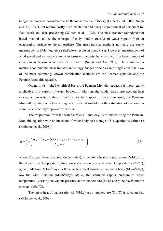
7.2. Method and data / 177
budget methods are considered to be the most reliable in theory (Lenters et al., 2005, Singh
and Xu, 1997), but require costly instrumentation and a large commitment of personnel for
field work and data processing (Winter et al., 1995). The mass-transfer (aerodynamic)
based methods utilize the concept of eddy motion transfer of water vapour from an
evaporating surface to the atmosphere. The mass-transfer methods normally use easily
measurable variables and give satisfactory results in many cases. However, measurement of
wind speed and air temperature at inconsistent heights, have resulted in a large number of
equations with similar or identical structure (Singh and Xu, 1997). The combination
methods combine the mass transfer and energy budget principles in a single equation. Two
of the most commonly known combination methods are the Penman equation and the
Penman-Monteith equation.
Owing to its limited empirical basis, the Penman-Monteith equation is more readily
applicable to a variety of water bodies. In addition, the model takes into account heat
storage within water bodies. Therefore, for the purpose of the current study the Penman-
Monteith equation with heat storage is considered suitable for the estimation of evaporation
from the selected hydropower reservoirs.
The evaporation from the water surface (E, mm/day) is estimated using the Penman-
Monteith equation with an inclusion of water body heat storage. This equation is written as
(McJannet et al., 2008):
+∆
−××+−×∆×=
γ)ee()u(fγ)GR(
λ1E
w
awnw (28)
where E is open water evaporation (mm/day); λ the latent heat of vaporization (MJ/kg); Δw
the slope of the temperature saturation water vapour curve at water temperature (kPa/oC);
Rn net radiation (MJ/m2/day); G the change in heat storage in the water body (MJ/m2/day);
f(u) the wind function (MJ/m2/day/kPa); ew the saturated vapour pressure at water
temperature (kPa); ea the vapour pressure at air temperature (kPa); and γ the psychometric
constant (kPa/oC).
The latent heat of vaporisation (λ, MJ/kg) at air temperature (Ta, oC) is calculated as
(McJannet et al., 2008):
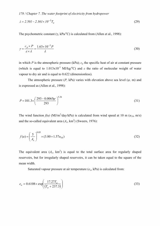
178 / Chapter 7. The water footprint of electricity from hydropower
a3T10361.2501.2λ −×−= (29)
The psychometric constant (γ, kPa/oC) is calculated from (Allen et al., 1998):
λλεγ PPc p
31063.1 −×=
×
×= (30)
in which P is the atmospheric pressure (kPa); cp the specific heat of air at constant pressure
(which is equal to 1.013x10⁻³ MJ/kg/oC) and ε the ratio of molecular weight of water
vapour to dry air and is equal to 0.622 (dimensionless).
The atmospheric pressure (P, kPa) varies with elevation above sea level (ψ, m) and
is expressed as (Allen et al., 1998):
26.5
2930065.02933.101
−
×=ψP (31)
The wind function f(u) (MJ/m2/day/kPa) is calculated from wind speed at 10 m (u10, m/s)
and the so-called equivalent area (Ae, km2) (Sweers, 1976):
)57.180.3(5)( 10
05.0
uA
ufe
+×
= (32)
The equivalent area (Ae, km2) is equal to the total surface area for regularly shaped
reservoirs, but for irregularly shaped reservoirs, it can be taken equal to the square of the
mean width.
Saturated vapour pressure at air temperature (ea, kPa) is calculated from:
( )
+
×=3.237
27.17exp6108.0a
aa T
Te (33)
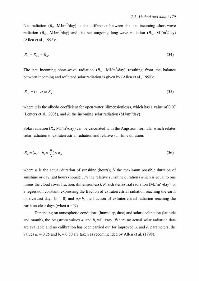
7.2. Method and data / 179
Net radiation (Rn, MJ/m2/day) is the difference between the net incoming short-wave
radiation (Rns, MJ/m2/day) and the net outgoing long-wave radiation (Rnl, MJ/m2/day)
(Allen et al., 1998):
nlnsn RRR −= (34)
The net incoming short-wave radiation (Rns, MJ/m2/day) resulting from the balance
between incoming and reflected solar radiation is given by (Allen et al., 1998):
sns RR ×−= )1( α (35)
where α is the albedo coefficient for open water (dimensionless), which has a value of 0.07
(Lenters et al., 2005), and Rs the incoming solar radiation (MJ/m2/day).
Solar radiation (Rs, MJ/m2/day) can be calculated with the Angstrom formula, which relates
solar radiation to extraterrestrial radiation and relative sunshine duration:
asss RNnbaR ××+= )( (36)
where n is the actual duration of sunshine (hours); N the maximum possible duration of
sunshine or daylight hours (hours); n/N the relative sunshine duration (which is equal to one
minus the cloud cover fraction, dimensionless); Ra extraterrestrial radiation (MJ/m2 /day); as
a regression constant, expressing the fraction of extraterrestrial radiation reaching the earth
on overcast days (n = 0) and as+bs the fraction of extraterrestrial radiation reaching the
earth on clear days (when n = N).
Depending on atmospheric conditions (humidity, dust) and solar declination (latitude
and month), the Angstrom values as and bs will vary. Where no actual solar radiation data
are available and no calibration has been carried out for improved as and bs parameters, the
values as = 0.25 and bs = 0.50 are taken as recommended by Allen et al. (1998).
180 / Chapter 7. The water footprint of electricity from hydropower
The extraterrestrial radiation, Ra, for each day of the year and for different latitudes, can be
estimated from the solar constant, the solar declination and the time of the year.
( ) ( ) ( ) ( ) ( )24 60 sin sin cos cos sina sc r s sR G d ω ϕ δ ϕ δ ωπ×
= × × × + × × (37)
where Gsc is the solar constant (which is equal to 0.0820 MJ/m2/day); dr the inverse relative
distance Earth-Sun; ω s the sunset hour angle (rad); ϕ the latitude (rad) and δ the solar
decimation (rad).
The inverse relative distance Earth-Sun, dr, and the solar declination, δ, are given by:
×+= Jdr 365
2cos033.01 π (38)
−×= 39.1
3652sin409.0 Jπδ (39)
where J is the number of the day in the year between 1 (1 January) and 365 or 366 (31
December). The latitude ϕ, expressed in radians, is positive for the northern hemisphere
and negative for the southern hemisphere.
The sunset hour angle, ωs, is given by:
)]δtan()φtan(arccos[ωs ×−= (40)
The net outgoing long-wave radiation (Rnl, MJ/m2/day) is the difference between the
outgoing long-wave radiation (Rl↑, MJ/m2/day) and the incoming long-wave radiation (Rl↓,
MJ/m2/day):
nl l lR R R= ↑ − ↓ (41)
7.2. Method and data / 181
The incoming long-wave radiation (Rl↓, MJ/m2/day) is calculated from (Fischer et al.,
1979; Henderson-Sellers, 1986):
( ) ( )( )lwfaal rCTR −++××↓= 117.0115.273 24σε (42)
where εa is the emissivity of air (dimensionless); σ the Stefan-Boltzmann constant
(4.903x10⁻⁹ MJ/K4/m2/day); Cf the fractional cloud cover (dimensionless); and rlw the total
reflectivity of the water surface for long wave radiation, taken as a constant with a value of
0.03 (Henderson-Sellers, 1986).
The emissivity of air is calculated as (Swinbank, 1963):
( )215.273+×= aa TCεε (43)
where Cε = 9.37×10⁻⁶ K-2.
The outgoing long-wave radiation at water temperature (Rl↑, MJ/m2/day) is calculated as
(Henderson-Sellers, 1986):
( )415.273+××↑= wwl TR σε (44)
where σ is the Stefan-Boltzmann constant (MJ/m2/K4/day); Tw the water surface
temperature (oC); and εw the emissivity of water, equal to 0.97.
The water temperature at day i (Twi, oC) is calculated from the following equation (De
Bruin, 1982):
( )τ1exp)TT(TT e1i,wei,w −×−+= − (45)
where Tw,i-1 is the water temperature at day i-1 (oC); Te the equilibrium temperature (oC);
and τ the time constant (day).
182 / Chapter 7. The water footprint of electricity from hydropower
The equilibrium temperature (Te, oC) is calculated as follows (De Bruin, 1982):
( ) ( ) ( )γuf15.273Tσ4RTT
n3
n
*n
ne+∆×++×
+= (46)
Wet-bulb temperature (Tn, oC) is calculated using vapour pressure (ea, kPa) and dew point
temperature (Td, oC) as follows (McJannet et al., 2008):
( )( )( )( )
2
2
0.00066 100 4098 / 237.3
0.00066 100 4098 / 237.3
a a d dn
a d
T e T TT
e T
× + + ×=
× + + (47)
The slope of the temperature saturation water vapour curve at wet bulb temperature (Δn,
kPa/K) is:
( )( )2n
n
n
n 3.237T
3.237TT27.17exp6108.04098
+
+
××
=∆ (48)
Net radiation at wet-bulb temperature ( *nR , MJ/m2/day) is calculated using albedo (α) as
follows:
( ) ( )nllsn RRRR ↑−↓+×−= α1* (49)
Outgoing long-wave radiation at wet-bulb temperature (Rl↑n, MJ/m2/day) is calculated,
based on Finch and Gash (2002):
( ) ( ) ( )( )anaafnl TTTTCR −×+×++××=↑ 34 15.273415.273 σσ (50)
where Cf is fractional cloud cover.
7.2. Method and data / 183
The time constant (τ, day) is given as (De Bruin, 1982):
( ) ( ) ( )γσρτ
+∆×++×
××=
nn
ww
ufThc
315.2734 (51)
where ρw is the density of water (= 1000 kg/m3); cw the specific heat of water (= 0.0042
MJ/kg/K); and h the depth of water (m), estimated from reservoir volume capacity and area.
Change in the heat storage in the water body (G, MJ/m2/day) is calculated from Finch
(2001):
( )1i,wi,www TThcρG −−×××= (52)
Saturated vapour pressure at water temperature (ew, kPa) is calculated from:
( )17.27
0.6108 exp237.3
ww
w
Te
T
= × + (53)
Finally, the slope of the temperature saturation water vapour curve at water temperature
(Δw, kPa oC-1) is:
( )( )23.237
3.23727.17exp6108.04098
+
+
××
=∆w
w
w
w T
TT
(54)
The water footprint of electricity from hydropower is compared with the water footprint of
electricity from combustion of primary crops. The latter has been calculated per type of
crop by first multiplying the water footprint of the primary crop in m3/ton from Mekonnen
and Hoekstra (2011a) by the harvest index for that crop to get the water footprint in m3 per
184 / Chapter 7. The water footprint of electricity from hydropower
ton of total biomass harvested. Harvest indices were taken from Gerbens-Leenes et al.
(2009a,b). Next, the water footprint of total biomass was divided by the bio-electricity
output per unit of crop (GJ/ton) as reported by Gerbens-Leenes et al. (2008a).
Data on installed hydroelectric capacity, actual hydroelectric generation and
reservoir area were obtained from the World Bank (1996). For some hydropower plants
data were obtained from Dorcey et al. (1997) and other sources. Data on reservoir water
holding capacity were obtained mainly from Chao et al. (2008).
Daily values of mean air temperature, dew point temperature and wind speed for the
selected meteorological stations were obtained from NCDC (2009). The daily data for the
years 1996-2005 were averaged in order to fill missing values and smooth out some
inconsistencies in the data. Monthly values of cloud cover and percentage of maximum
possible sunshine with a spatial resolution of 10 arc minute were obtained from the CRU
CL-2.0 database (New et al., 2002). The cloud cover and sunshine duration were available
only as monthly averages for the period 1961-1990. Therefore the monthly average values
were used as daily values for each month of the year.
7.3 Results: the water footprint of hydroelectricity
The aggregated blue water footprint of the 35 selected hydropower plants is 90 Gm3/yr,
which is equivalent to 10% of the blue water footprint of global crop production in the year
2000 (Mekonnen and Hoekstra, 2011a; Fader et al., 2011). The total blue water footprint of
hydroelectric generation in the world must be considerably larger if one considers the fact
that this study covers only 8% of the global installed hydroelectric capacity. The annual
evaporation from hydropower reservoirs depends on both climate (which determines the
evaporation from the water surface in mm/yr) and reservoir area.
The water footprint of electricity from hydropower for the 35 selected hydropower
plants is presented in Table 7.1. The average water footprint of electricity from hydropower
for the selected plants is 68 m3/GJ. There is a large variation in water footprint among the
different power plants, ranging from 0.3 m3/GJ for San Carlos in Colombia to 846 m3/GJ
for Akosombo-Kpong in Ghana.
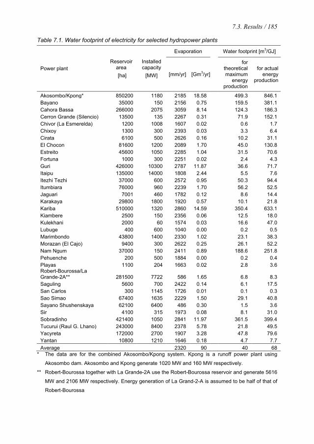
7.3. Results / 185
Table 7.1. Water footprint of electricity for selected hydropower plants
Power plant Reservoir
area [ha]
Installed capacity
[MW]
Evaporation Water footprint [m3/GJ]
[mm/yr] [Gm3/yr]
for theoretical maximum
energy production
for actual energy
production
Akosombo/Kpong* 850200 1180 2185 18.58 499.3 846.1 Bayano 35000 150 2156 0.75 159.5 381.1 Cahora Bassa 266000 2075 3059 8.14 124.3 186.3 Cerron Grande (Silencio) 13500 135 2267 0.31 71.9 152.1 Chivor (La Esmerelda) 1200 1008 1607 0.02 0.6 1.7 Chixoy 1300 300 2393 0.03 3.3 6.4 Cirata 6100 500 2626 0.16 10.2 31.1 El Chocon 81600 1200 2089 1.70 45.0 130.8 Estreito 45600 1050 2285 1.04 31.5 70.6 Fortuna 1000 300 2251 0.02 2.4 4.3 Guri 426000 10300 2787 11.87 36.6 71.7 Itaipu 135000 14000 1808 2.44 5.5 7.6 Itezhi Tezhi 37000 600 2572 0.95 50.3 94.4 Itumbiara 76000 960 2239 1.70 56.2 52.5 Jaguari 7001 460 1782 0.12 8.6 14.4 Karakaya 29800 1800 1920 0.57 10.1 21.8 Kariba 510000 1320 2860 14.59 350.4 633.1 Kiambere 2500 150 2356 0.06 12.5 18.0 Kulekhani 2000 60 1574 0.03 16.6 47.0 Lubuge 400 600 1040 0.00 0.2 0.5 Marimbondo 43800 1400 2330 1.02 23.1 38.3 Morazan (El Cajo) 9400 300 2622 0.25 26.1 52.2 Nam Ngum 37000 150 2411 0.89 188.6 251.8 Pehuenche 200 500 1884 0.00 0.2 0.4 Playas 1100 204 1663 0.02 2.8 3.6 Robert-Bourossa/La Grande-2A** 281500 7722 586 1.65 6.8 8.3 Saguling 5600 700 2422 0.14 6.1 17.5 San Carlos 300 1145 1726 0.01 0.1 0.3 Sao Simao 67400 1635 2229 1.50 29.1 40.8 Sayano Shushenskaya 62100 6400 486 0.30 1.5 3.6 Sir 4100 315 1973 0.08 8.1 31.0 Sobradinho 421400 1050 2841 11.97 361.5 399.4 Tucurui (Raul G. Lhano) 243000 8400 2378 5.78 21.8 49.5 Yacyreta 172000 2700 1907 3.28 47.8 79.6 Yantan 10800 1210 1646 0.18 4.7 7.7 Average 2320 90 40 68
* The data are for the combined Akosombo/Kpong system. Kpong is a runoff power plant using
Akosombo dam. Akosombo and Kpong generate 1020 MW and 160 MW respectively.
** Robert-Bourossa together with La Grande-2A use the Robert-Bourossa reservoir and generate 5616
MW and 2106 MW respectively. Energy generation of La Grand-2-A is assumed to be half of that of
Robert-Bourossa
186 / Chapter 7. The water footprint of electricity from hydropower
Most of the reservoirs show an evaporation rate between 2000 and 3000 mm/yr. Reservoirs
in the tropics have generally a higher evaporation rate than reservoirs in temperate and sub-
tropic climatic regions. The surface water evaporation varies from no more than 486 mm/yr
from the Sayano Shushenskaya reservoir in Russia to 3059 mm/yr from the Cahora Bassa
reservoir in the Zambezi River in Mozambique (Table 7.1). Minimum and maximum
evaporation rates thus differ by a factor of six, which partially explains the differences
between the water footprints of different hydropower reservoirs. The size of the reservoir
surface in relation to the installed hydroelectric capacity, however, has a much bigger
impact on the ultimate water footprint of hydroelectricity. While the average reservoir area
per unit of installed capacity in the reservoirs studied is 83 ha/MW, the minimum is 0.26
ha/MW (San Carlos reservoir, Colombia) and the maximum 720 ha/MW (Akosombo-
Kpong in the Volta River, Ghana). The total evaporation from a hydropower reservoir thus
depends more on its size than on climate. This is illustrated in Figure 7.1, which shows a
more or less linear relationship between the water footprint of the power plants and
ha/MW. Hydropower plants that inundate a large area per unit of installed capacity have in
general a larger water footprint per unit of electricity generated than those that flood a small
area per unit of installed capacity.
The largest hydropower plant in terms of installed hydroelectric capacity in this
study, the Itaipu dam in the Paraná River at the border of Brazil and Paraguay, has a water
footprint of 7.6 m3/GJ. The second-largest studied hydropower plant in terms of MW, the
Guri reservoir in Venezuela, has a water footprint that is close to the global average of 68
m3/GJ found in this study. The largest plant in terms of MW that has a water footprint far
beyond the average found in this study is the Cahora Bassa dam in the Zambezi River in
Mozambique, with a water footprint of 186 m3/GJ.
When we compare the water footprint of electricity from hydropower with the water
footprint of electricity from other renewable sources, it appears that hydroelectricity has a
relatively large water footprint per GJ. The blue water footprint of electricity from wind
and solar energy is estimated to be well below 1 m3/GJ (Gerbens-Leenes et al., 2009a). The
blue water footprint of bio-electricity – when derived from combustion of the full biomass
of primary crops – ranges from zero to 40 m3/GJ, depending on which crop is used for
comparison and to which extent it is irrigated. The 40 m3/GJ refers to bio-electricity from
combustion of cotton, which is a rather theoretical example, because cotton is in practice

7.3. Results / 187
not used for the purpose of electricity generation. Also other crops are rarely used for that
purpose. More common feedstock for the generation of bio-electricity are crop residues,
animal manure, wood wastes from forestry and industry, residues from food and paper
industries, municipal green wastes and sewage sludge. In all those cases, the water footprint
of bio-electricity will be much lower than the water footprint of bio-electricity from
combustion of primary crops, because the water footprint of biomass is largely attributed to
the primary product and not to the residues and waste (Hoekstra et al., 2011).
0
40
80
120
0 10 20 30 40 50 60 70 80
Wat
er fo
otpr
int [
m3 /G
J]
Flooded area per unit of installed capacity [ha/MW]
R² = 0.9538
0
200
400
600
800
1000
0 100 200 300 400 500 600 700 800
Wat
er f
ootp
rint [
m3 /
GJ]
Flooded area per unit of installedcapacity [ha/MW]
Akosombo
Kariba
Sobradinho
Nam Ngum
Bayano
Yacyreta
Itezhi Tezhi
Sao Simao
Robert-Bourossa
San Carlos
Figure 7.1. Relation between water footprint of hydroelectricity and flooded area per unit of installed hydroelectric capacity.
Figure 7.2 compares the blue water footprint of electricity from hydropower with the total
(green+blue+grey) water footprint of electricity from combustion of primary crops. For a
fair comparison one should compare the blue water footprints. But even when comparing
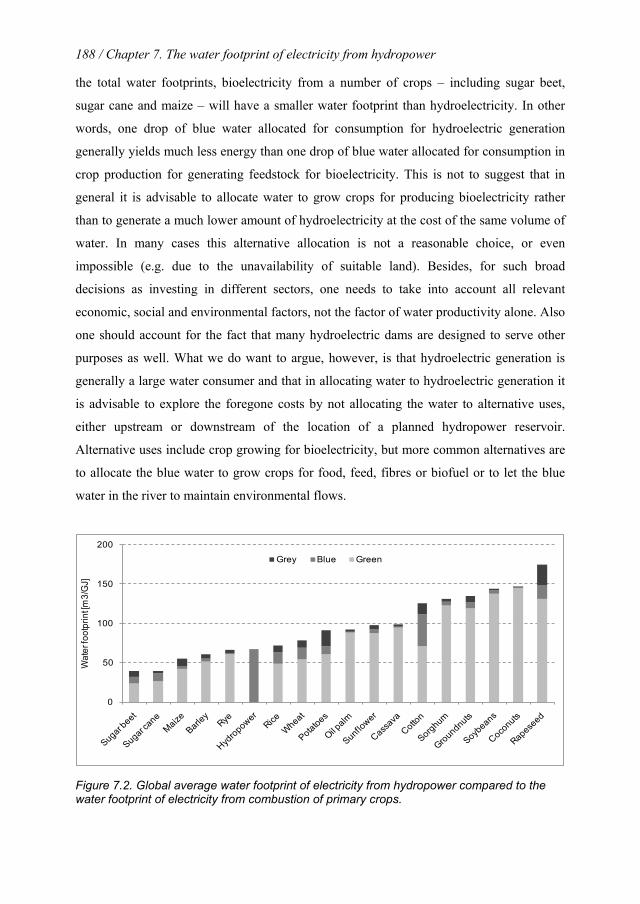
188 / Chapter 7. The water footprint of electricity from hydropower
the total water footprints, bioelectricity from a number of crops – including sugar beet,
sugar cane and maize – will have a smaller water footprint than hydroelectricity. In other
words, one drop of blue water allocated for consumption for hydroelectric generation
generally yields much less energy than one drop of blue water allocated for consumption in
crop production for generating feedstock for bioelectricity. This is not to suggest that in
general it is advisable to allocate water to grow crops for producing bioelectricity rather
than to generate a much lower amount of hydroelectricity at the cost of the same volume of
water. In many cases this alternative allocation is not a reasonable choice, or even
impossible (e.g. due to the unavailability of suitable land). Besides, for such broad
decisions as investing in different sectors, one needs to take into account all relevant
economic, social and environmental factors, not the factor of water productivity alone. Also
one should account for the fact that many hydroelectric dams are designed to serve other
purposes as well. What we do want to argue, however, is that hydroelectric generation is
generally a large water consumer and that in allocating water to hydroelectric generation it
is advisable to explore the foregone costs by not allocating the water to alternative uses,
either upstream or downstream of the location of a planned hydropower reservoir.
Alternative uses include crop growing for bioelectricity, but more common alternatives are
to allocate the blue water to grow crops for food, feed, fibres or biofuel or to let the blue
water in the river to maintain environmental flows.
0
50
100
150
200
Wat
er fo
otpr
int [m
3/G
J]
Grey Blue Green
Figure 7.2. Global average water footprint of electricity from hydropower compared to the water footprint of electricity from combustion of primary crops.

7.4. Discussion / 189
7.4 Discussion
The water footprints of the artificial reservoirs analysed in this study were fully attributed
to hydroelectric generation, even though some of the reservoirs serve other purposes as
well, such as flood control and irrigation. We justify this choice by the fact that all selected
hydropower dams and associated reservoirs were primarily created for hydroelectric
generation. Future research could be directed towards the analysis of the water footprint of
reservoirs created for storing water for irrigation or other purposes and on tackling the
water footprint attribution issue when reservoirs are used for multiple purposes.
The model output is sensitive to a number of input parameters such as air
temperature, wind speed and water body depth. Since climatic data at the dam site are
available only for a few plants, data from the most nearby climatic stations have been used,
some of which are a bit far from the reservoir. Due to the uncertainties in the input data, the
data presented should be seen as indicative. The order of magnitude of the results, however,
will not change with better data, so that the results are good enough to compare the water
footprint of hydroelectricity with the water footprint of other forms of electricity and to
make rough comparisons between the water footprints of different hydropower sites.
Most reservoirs have a varying water surface area over time, as a result of changes in
water volume during the year and between years. The difference between minimum and
maximum area relative to the maximum area over a multi-year period differs greatly across
reservoirs. In this study we have used a fixed reservoir area as provided by World Bank
(1997) and Dorcey et al. (1997). Since reported areas generally refer to the maximum, this
can lead to some overestimation of evaporation over the year. It is very difficult to find
good data of area changes over the year; future studies devoted to particular sites could
improve this.
We have estimated the water footprint per reservoir by considering the total
evaporation from the reservoir, whereas one could argue that before the reservoir was
created there was evaporation from the area as well, probably not so much from the original
flowing river (since in most cases the reservoir area is much larger than the original river
water area) but possibly significant from the inundated land. However, here it is relevant to
recall the definition and meaning of the water footprint. The water footprint is not meant to
refer to additional evaporation (compared to some reference situation), but for quantifying
190 / Chapter 7. The water footprint of electricity from hydropower
the volume of water consumption that can be associated with a specific human purpose
(Hoekstra et al., 2011). From this perspective, the full reservoir evaporation can be
attributed to the purpose of the reservoir.
The study has been limited to the estimation of the evaporation from reservoirs, i.e.
the so-called operational water footprint of hydroelectric generation. The study does not
include an assessment of the supply-chain water footprint of hydroelectric generation,
which is expected to be much smaller than the operational water footprint. The supply-
chain water footprint refers to the water footprint of producing the materials used in the
construction and the operation and maintenance of the site.
The current study does not claim to be exhaustive in terms of showing both the
beneficial and negative effects of hydropower. The study has been restricted to the
estimation of the water footprint of different hydropower plants. Environmental issues
surrounding hydropower dams relate to, for example: physical, chemical, biological and
geomorphological aspects of blocking a river; flooding of natural habitats and related loss
of plants and animals; alteration of water flow regimes; and water quality problems due to
the decay of submerged vegetations. On the other hand, hydropower is often perceived as a
clean and cost-effective source of renewable energy. Many countries rely upon hydropower
for a substantial portion of their electricity supply. Between 1973 and 2008, hydroelectric
generation grew from 1295 TWh to 3288 TWh, which is a growth by a factor 2.5 (IEA,
2010). Further development of hydropower should take into account all the associated
environmental and social costs. In this respect, the water footprint of hydroelectricity, i.e.
the consumptive use of water, should be considered as one item in environmental impact
assessment studies for newly proposed hydroelectric dams.
7.5 Conclusion
Hydroelectric generation has historically been considered as a non-consumptive water user;
however, through the estimation of the blue water footprint of hydroelectricity at 35 sites,
this study finds that hydropower is a large consumptive user of water. The amount of water
lost through evaporation annually from the selected reservoirs is equivalent to 10% of the
global blue water footprint related to crop production. The 35 sites represent only 8% of the
global installed hydroelectric capacity. The study shows that the range of water footprint
7.5. Conclusion / 191
values for the different hydropower plants is very wide. Although local climate has an
influence, the water footprint of hydroelectricity is largely influenced by the area flooded
per unit of installed capacity. The water footprint linearly increases with the area flooded
per unit of installed capacity.
The water evaporated from the reservoir is seldom taken into account in assessing
the pros and cons of constructing dams for hydroelectric generation. This study
demonstrates that accounting for water loss through evaporation is an additional
consideration when evaluating the environmental, social and economic sustainability of a
proposed dam or in the evaluation of hydropower as an energy source. We recommend that
water footprint assessment is added as a component in evaluations of newly proposed
hydropower plants as well as in the evaluation of existing hydroelectric dams, so that the
consequences of the water footprint of hydroelectric generation on downstream
environmental flows and other water users can be evaluated.
The water footprint of hydroelectric dams should be considered in the context of the
river basin in which this water footprint occurs, because competition over water and
possible alternative uses of water differ per basin. This study contributes new information
that can be used in river basin planning and water allocation decisions.
Sustainable development of hydropower requires the accounting and internalization
of all external costs including water consumption. Internalization means that the economic
and environmental costs of the water consumed are charged to the operator of a
hydropower plant and included in the price of hydroelectricity. It should thereby be
acknowledged that water consumption costs vary within the year and across river basins,
since the degree of water scarcity and competition over water depend on the period within
the year and local circumstances.

8. The external water footprint of the Netherlands: geographically-explicit quantification and impact assessment7
Abstract
This study quantifies the external water footprint of the Netherlands by partner country and
import product and assesses the impact of this footprint by contrasting the geographically
explicit water footprint with water scarcity in the different parts of the world. The total
water footprint of the Netherlands is estimated to be about 2300 m3/yr/cap, of which 67%
relates to the consumption of agricultural goods, 31% to the consumption of industrial
goods, and 2% to domestic water use. The Dutch water footprint related to the consumption
of agricultural goods, is composed as follows: 46% related to livestock products; 17% oil
crops and oil from oil crops; 12% coffee, tea, cocoa and tobacco; 8% cereals and beer; 6 %
cotton products; 5% fruits; and 6 % other agricultural products. About 11% of the water
footprint of the Netherlands is internal and 89% is external. Only 44% of the virtual-water
import relates to products consumed in the Netherlands, thus constituting the external water
footprint. For agricultural products this is 40% and for industrial products this is 60%. The
remaining 56% of the virtual-water import to the Netherlands is re-exported. The impact of
the external water footprint of Dutch consumers is highest in countries that experience
serious water scarcity. Based on indicators for water scarcity the following eight countries
have been identified as hotspots: China; India; Spain; Turkey; Pakistan; Sudan; South
Africa; and Mexico. The study shows that Dutch consumption implies the use of water
resources throughout the world, with significant impacts at specified locations.
8.1 Introduction
The background of this study is the recognition that there is a relation between consumption
by Dutch consumers and impacts on water systems elsewhere in the world. Many of the
goods consumed in the Netherlands are not produced in the Netherlands, but abroad. Some
goods, most in particular agriculture-based products, require a lot of water during
7 Based on Van Oel, P.R. et al. (2008, 2009).

194 / Chapter 8. The external water footprint of the Netherlands
production. These water-intensive production processes are accompanied by impacts on the
water systems at the various locations where the production processes take place. The
impacts vary from reduced river water flows, declined lake levels and declined ground
water tables to increased salt intrusion in coastal areas and pollution of freshwater bodies.
As an indicator of the water use related to consumption we use the water footprint concept.
The water footprint of a nation is defined as the total amount of freshwater that is used to
produce the goods and services consumed by the inhabitants of the nation (Hoekstra and
Chapagain, 2007a, 2008). The total water footprint of a country includes two components:
the part of the footprint that falls inside the country (internal water footprint) and the part of
the footprint that presses on other countries in the world (external water footprint). In this
study, we focus on the external water footprint of the Netherlands.
The external water footprint of the Netherlands is the volume of water used in other
countries to produce goods and services imported and consumed by the inhabitants of the
Netherlands. The water footprint is a quantitative measure of the amount of water
consumed. It breaks down into three components: the blue, green and grey water footprint.
The blue water footprint is the volume of freshwater that evaporated from the global blue
water resources (surface water and ground water) to produce the goods and services
consumed by the people in a nation. The green water footprint is the volume of water
evaporated from the global green water resources (rainwater stored in the soil as soil
moisture). The grey water footprint is the volume of polluted water that associates with the
production of all goods consumed in the nation. The latter is calculated as the volume of
water that is required to dilute pollutants to such an extent that the quality of the water
remains above agreed water quality standards. Analysis of the grey water footprint of the
Dutch community will be done in this study only in the last phase, when analyzing the
impacts at hotspots.
The external water footprint of the Netherlands is specified according to (i) partner
countries and (ii) imported products. The results of the country and product analyses are
confronted with water scarcity indicators. In this way, hotspots are identified where the
external water footprint of the Netherlands expectedly has the largest impacts. For a
number of selected hotspots the impact on the affected local water systems will be further
analyzed. The research is driven by the following research questions: What is the water use
outside of the Dutch borders in effect of Dutch consumption? In which countries is the
8.2. Method / 195
external footprint concentrated? What are the main products related to this external
footprint? What is the external water footprint related to total water use behind imports into
the Netherlands? In which countries is the impact of the external water footprint most
serious (hotspots)? What are the impacts of the external water footprint on local water
systems in the identified hotspots?
We have considered the period 1996-2005, which is long enough to get a good
impression of average Dutch trade and its effects on the Dutch water footprint, excluding
the effects of deviations in specific years, but which is not long enough to carry out trend-
analyses, which was out of the scope of the current study. In quantifying the total external
water footprint of the Netherlands it was not feasible to distinguish between the green, blue
and grey components of the water footprint, but in the analysis of the identified hotspots, a
specification of the green, blue and grey water footprint was made.
8.2 Method
As defined by Hoekstra and Chapagain (2007a, 2008), the water footprint (WFcons) of Dutch
consumers has two components: the internal water footprint (WFcons,int) and the external
water footprint (WFcons,ext):
]NL[WF]NL[WF]NL[WF ext,consint,cons += (55)
The internal water footprint is defined as the annual use of domestic water sources to
produce goods and services consumed by the Dutch population. It is the sum of the total
water volume used from the domestic water resources in the national economy (WFarea)
minus the volume of virtual-water export to other countries insofar as related to the export
of products produced with national water resources (Ve,d):
]NL[V]NL[WF]NL[WF d,eareaint,cons −= (56)
The external water footprint is defined as the annual volume of freshwater resources used in
other countries to produce goods and services consumed by the population of these
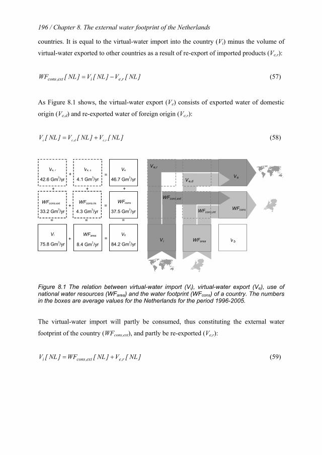
196 / Chapter 8. The external water footprint of the Netherlands
countries. It is equal to the virtual-water import into the country (Vi) minus the volume of
virtual-water exported to other countries as a result of re-export of imported products (Ve,r):
]NL[V]NL[V]NL[WF r,eiext,cons −= (57)
As Figure 8.1 shows, the virtual-water export (Ve) consists of exported water of domestic
origin (Ve,d) and re-exported water of foreign origin (Ve,r):
]NL[V]NL[V]NL[V r,ed,ee += (58)
Figure 8.1 The relation between virtual-water import (Vi), virtual-water export (Ve), use of national water resources (WFarea) and the water footprint (WFcons) of a country. The numbers in the boxes are average values for the Netherlands for the period 1996-2005.
The virtual-water import will partly be consumed, thus constituting the external water
footprint of the country (WFcons,ext), and partly be re-exported (Ve,r):
]NL[V]NL[WF]NL[V r,eext,consi += (59)
V i
WFarea
V e,r
WFcons,int
WFcons
V e
WFcons,ext
V e,d
V b
V e 46.7 Gm 3 /yr
WFcons 37.5 Gm 3 /yr
WFarea 8.4 Gm 3 /yr
V i 75.8 Gm 3 /yr
V b 84.2 Gm 3 /yr
V e, d 4.1 Gm 3 /yr
WFcons,int 4.3 Gm 3 /yr
WFcons,ext
33.2 Gm 3 /yr
V e, r 42.6 Gm 3 /yr
+
+
=
=
+ +
= =
+ =
=
+
8.2. Method / 197
Finally, we see in Figure 8.1 that the sum of Vi and WFarea is equal to the sum of Ve and
WFcons. We call this sum the virtual-water budget (Vb) of a country (Ma et al., 2006;
Hoekstra and Chapagain, 2008).
]NL[WF]NL[V]NL[WF]NL[V]NL[V
conse
areaib
+=+=
(60)
The water footprint (WFcons) of a country can be estimated through a bottom-up or top-
down approach. In this study both approaches are applied in order to be able to compare the
outcomes. As will become clear, however, the bottom-up approach gives more reliable
results in the case of the Netherlands, so that in the rest of the study, after the comparison of
the outcomes of both approaches, we will work with the outcomes of the bottom-up
approach.
8.2.1 Bottom-up approach
In the bottom-up approach, the water footprint (WFcons) of the Netherlands (NL) is
calculated by adding the direct water use by people and their indirect water use:
]NL[WF]NL[WF]NL[WF indir,consdir,conscons += (61)
The direct water use refers to the water that people consume at home. The indirect water
use of people refers to the water use by others to make the goods and services consumed. It
refers to the water that was used to produce for example the food, clothes, paper, energy
and industrial goods consumed. The indirect water use is calculated by multiplying all
goods and services consumed by the inhabitants of the Netherlands by the respective water
needs for those goods and services:
( )∑=
×=n
1pindir,cons ]p,NL[*WF]p,NL[C]p,NL[WF (62)

198 / Chapter 8. The external water footprint of the Netherlands
C [NL,p] is Dutch consumption of product p (unit/yr) and WF*[NL,p] the water footprint
(virtual water content) of this product (m3/unit). The set of products considered refers to the
full range of final consumer goods and services. The water footprint (virtual water content)
of a product is the volume of freshwater used to produce the product, measured at the place
where the product was actually produced. The water footprint of a product thus varies as a
function of place and conditions of production. It refers to the sum of the water use in the
various steps of the production chain. The adjective ‘virtual’ refers to the fact that most of
the water used to produce a product is not contained in the product. The real-water content
of products is generally negligible if compared to the virtual water content. The water
footprint of individual primary and processed products is calculated (per country) based on
the method described in Hoekstra and Chapagain (2008).
In the case of agricultural products, the water footprint is expressed in terms of
m3/ton and consumption is expressed in ton/yr. In the case of industrial products, the water
footprint is, for practical reasons, expressed in terms of m3/US$ instead of m3/ton.
Industrial products show a relatively high heterogeneity and there are often different
production methods for one type of product. As a result, the weight of an industrial product
is not an as obvious indicator of underlying water use as in the case of an agricultural
product. Since industrial production in a sector as a whole is generally expressed in
monetary terms, it is easiest to consider water use in a sector per monetary unit as well.
The total volume of a product (p) consumed in a country will generally originate
from different nations (ne). The average water footprint of a product consumed in the
Netherlands is estimated by assuming that:
( )
∑
∑
=
=
+
×+×
= m
1cei
m
1cei
*
p],[nTp],P[NL
p],WF[cp],[nT]p,NL[WF]p,NL[Pp],[NLWF (63)
The assumption here is that consumption originates from domestic production (P, tons/yr)
and imports (Ti, tons/yr) according to their relative volumes.
8.2. Method / 199
8.2.2 Top-down approach
Another way of assessing the water footprint of a country (WFcons, m3/yr) is the top-down
approach, which takes the total water footprint (WFarea) in the country as starting point and
then adds the incoming virtual-water flow (Vi) and subtracts the virtual-water export (Ve):
]NL[V]NL[V]NL[WF]NL[WF eiareacons −+= (64)
The water use in the Netherlands is calculated as follows:
∑=
×=n
1parea ]p,NL[WF]p,NL[P]NL[WF (65)
The gross virtual-water import is calculated based on the imported quantity and the water
footprint of all products and countries:
∑∑= =
×=n
1p
m
1ceeii ,p]WF[n,p][nT[NL]V (66)
The gross virtual-water export is calculated based on the exported quantity (Te, tons/yr) and
the average water footprint of all products exported from the Netherlands:
∑=
×=n
1pee WF*[NL,p][NL,p]T[NL]V (67)
The average water footprint of an exported product is estimated by applying the same
assumption that was used in the bottom-up approach (equation (63)).
The bottom-up and top-down calculations of the water footprint of a country for a
particular year theoretically result in the same figure, provided that there is no product
stock change over a year. The top-down calculation can theoretically give a slightly higher

200 / Chapter 8. The external water footprint of the Netherlands
(lower) figure if the stocks of water-intensive products increase (decrease) over the year.
The reason is that the top-down approach presupposes a balance (Vi plus WFarea becomes
WFcons and Ve) which is an approximation only (to be more precise: Vi plus WFarea becomes
WFcons plus Ve plus virtual-water stock increase). Another drawback of the top-down
approach is that there can be delays between the moment of water use for production and
the moment of trade. For instance in the case of trade in livestock products this may
happen: beef or leather products traded in one year originate from livestock raised and fed
in previous years. Part of the water virtually embedded in beef or leather refers to water that
was used to grow feed crops in previous years. As a result of this, the virtual-water balance
presumed in the top-down approach ( ]NL[V]NL[WF]NL[V]NL[WF econsiarea +=+ )
will hold over a period of a few years, but not necessarily over one year.
Next to theoretical differences between the two approaches, differences can result
from the use of different types of data as inputs of the calculations. The bottom-up
approach depends on the quality of consumption data, while the top-down-approach relies
on the quality of trade data. When the different databases are not consistent with one
another, the results of both approaches will differ.
In one particular type of case the outcome of the top-down can be very vulnerable to
relatively small errors in the input data. This happens when the import and export of a
country are large relative to its domestic production, which is typical for a trade nation as
the Netherlands. In this case the water footprint, calculated in the top-down approach as the
domestic water use plus the virtual-water import minus the virtual-water export, will be
sensitive to the import and export data used. Relative small errors in the estimates of
virtual-water import and export translate into a relatively large error in the water footprint
estimate. In such a case, the bottom-up approach will yield a more reliable estimate than the
top-down approach. In countries where trade is relatively small compared to domestic
production, the reliability of the outcomes of both approaches will depend on the relative
quality of the databases used for each approach. In the case of agricultural products, both
calculations are carried out in this study. However, the water footprint outcomes from the
bottom-up approach are used as a basis for further analysis. For industrial products only
top-down calculations are carried out. In the case of industrial products, no distinction
between different types of industrial commodities is made, thus effectively industrial
8.2. Method / 201
products are regarded as one homogeneous category with an average water footprint per
dollar.
In the present study we are interested in the external water footprint of Dutch
consumers (WFcons,ext) and the re-exported virtual-water (Ve,r). To determine these terms we
use the following assumption, which we apply separately for the category of agricultural
products and for the category of the industrial products:
[NL]V[NL]WF[NL]V
[NL]WF[NL]WF iareai
consext,cons ×
+= (68)
This formula says that only a fraction of the gross virtual-water import can be said to be the
external water footprint of the Dutch consumers and that this fraction is equal to the portion
of virtual-water import plus use of domestic water that is to be attributed to consumption
within the country8.The other portion of virtual-water import plus use of domestic water is
exported and is therefore not part of the Dutch footprint. The term WFcons in above equation
refers to the water footprint of the Dutch consumers. When calculating the external water
footprint, the total water footprint as earlier calculated with the bottom-up approach has
been taken. The external water footprint can be estimated for specific countries and
products by assuming that the national ratio between the external water footprint and the
total virtual-water import applies to all partner countries and imported products9,10:
p],n,[NLV[NL]V
[NL]WFp],n,[NLWF ei
i
ext,conseext,cons ×= (69)
The external water footprint of Dutch consumers for an individual country and an
individual product are respectively:
8 This assumption implies that
eVconsWF
de,Vintcons,WF
re,Vextcons,WF
== and areaWFiV
de,Vre,V
intcons,WFextcons,WF
== .
9 We have made an exception for cocoa products and derivates, because of the exceptionally high volumes that are imported and re-exported again. The national ratio between WFcons,ext and Vi is not a good assumption here. Instead, we have applied a specific ratio of WFcons,ext to Vi valid to the cocoa product category.
10 For cotton we applied the top-down approach for estimating the water footprint, because data on cotton product consumption are not available in the consumption database used in this study (FAO, 2007b). Because the Netherlands does not have cotton production, we could now assume that WFcons,ext = Vi – Ve.
202 / Chapter 8. The external water footprint of the Netherlands
∑=
=n
1peext,conseext,cons p],[NL,nWF][NL,nWF (70)
∑=
=m
1neext,consext,cons
e
p],[NL,nWF[NL,p]WF (71)
Many products are imported from countries in which they are not produced. Examples are
cocoa products from Belgium and cotton products from Germany. For some product
groups, world production is concentrated in specific regions. For these products we can
estimate the ultimate place of origin based on world production data (FAO, 2010a). We do
this for cotton, cocoa and coffee. For these products it is assumed that the water footprint in
a non-producing country should be distributed over producing countries according to the
same distribution of the world production. We only include producing countries from
which the Netherlands is already importing directly.
8.2.3 Impact of the water footprint
In order to gather insight into the impacts of both Dutch consumption and re-exported
virtual-water, both WFcons,ext, and Vi as a whole are compared to indicators of water scarcity
or stress. Water-scarcity indicators are always based on two basic ingredients: a measure of
water demand or use and a measure of water availability.
The first commonly used indicator of water scarcity is population of an area divided
by total runoff in that area, called the water competition level (Falkenmark, 1989) or water
dependency (Kulshreshtha, 1993). Many authors take the inverse ratio, thus getting a
measure of the per capita water availability. Falkenmark proposed to consider regions with
more than 1700 m3 per capita per year as ‘water sufficient’, which means that only general
water management problems occur. Between 1000-1700 m3/cap/yr would indicate ‘water
stress’, 500-1000 m3/cap/yr ‘chronic water scarcity’ and less than 500 m3/cap/yr ‘absolute
water scarcity’. This classification is based on the idea that 1700 m3 of water per capita per
year is sufficient to produce the food and other goods and services consumed by one
person. In Falkenmark’s indicator ‘runoff’ is taken as a measure of water availability.

8.2. Method / 203
Runoff can refer to locally generated runoff (in FAO terminology then called the internal
renewable water resources, IRWR), but it can also include inflows from other areas (in
FAO terminology then called the total renewable water resources, TRWR).
A second common indicator of water scarcity is the ratio of water withdrawal in a
certain area to total runoff in that area, called variously the water utilization level
(Falkenmark, 1989; Falkenmark et al., 1989), the withdrawal-to-availability ratio (Alcamo
et al., 2000, 2002) or the use-to-resource ratio (Raskin et al., 1996).
The third indicator has been proposed by Smakhtin et al. (2004a; 2004b), who have
determined the withdrawal-to-availability ratio by basin.
All three water scarcity indicators can be applied to either countries or river basins.
The indicators of water scarcity enable us to estimate the Dutch share in the creation of
water stress in a country. On weak soil the imprint of a footstep is deeper than that it is on
solid ground, so the impact of a water footprint in a water-scarce area is larger than in an
area where water is more abundant.
8.2.4 Green, blue and grey water footprint
For the products with the largest contribution to the external water footprint of the
Netherlands in the identified hotspots we estimate the size of the green, blue and grey
components in the total water footprint.
In the case of agricultural products, we estimate the volume of green water use by
taking the minimum of the crop water requirement and the precipitation available to the
crop over the cropping season. We assume that 60% of the rainfall in the cropping season is
available to the crop. The difference between crop water requirement and the precipitation
available to the crop over the cropping season gives an indication of the irrigation water
requirement (i.e. blue water requirement). For the areas equipped for irrigation it is
assumed that the irrigation water requirements were actually met. For estimating the green
versus blue water footprint in agriculture, the following spatial-explicit data have been
used:
- The main locations where specific crops are cultivated (e.g. Leff et al., 2004);
- The percentage of land equipped for irrigation (Döll and Siebert 2000);
- Crop water requirements (Hoekstra and Chapagain, 2008).
204 / Chapter 8. The external water footprint of the Netherlands
- Monthly precipitation at meteorological station (Müller and Hennings, 2000).
In the case of agricultural products, estimation of the grey water footprint is done as
follows. It is assumed that the quantity of nitrogen that reaches free flowing water bodies is
10% of the applied fertilization rate (in kg/ha/yr), presuming a steady state balance at root
zone in the long run (Hoekstra and Chapagain, 2008). The effect of the use of other
nutrients, pesticides and herbicides to the environment has not been analyzed. The total
volume of water required per ton N is calculated considering the volume of nitrogen
leached (ton/ton) and the maximum allowable concentration in the free flowing surface
water bodies. The standard recommended by EPA (2005) for nitrate in drinking water is 10
milligrams per litre (measured as nitrogen) and has been taken to calculate the necessary
dilution water volume. This is a conservative approach, since natural background
concentration of N in the water used for dilution has been assumed negligible. Data on the
application of fertilizers has been obtained from the FERTISTAT database of FAO (FAO,
2010c).
In the case of industrial products data on water withdrawals from FAO (2010b) have
been used. Part of this volume evaporates (blue water footprint), while the other part
generally returns as polluted water to the water system (grey water footprint). In the cases
where industrial wastewater flows are partially treated, we have thus overestimated the grey
water footprint. On the other hand, the effect of pollution has been underestimated, because
one cubic meter of wastewater generally does not result in one cubic metre of polluted
water, but much more (Postel et al., 1996). On average, ten percent of industrial water
withdrawals are lost through evaporation (Shiklomanov and Rodda, 2003). In this paper we
assume that in the estimated water footprints related to industrial products, ten percent is a
blue water footprint and ninety percent is a grey water footprint.
Results of this study are based on data for the period of 1996-2005. Most results are
presented as 10-year averages, although in some cases specific annual data are shown. The
product coverage of the study is comprehensive: the trade analysis covers all agricultural
and industrial product categories as represented in the trade database of ITC (2007) and the
consumption analysis covers all consumption categories available within the food balance
sheets of the FAO (2010a). Table 8.1 gives an overview of all input sources used in this
study.
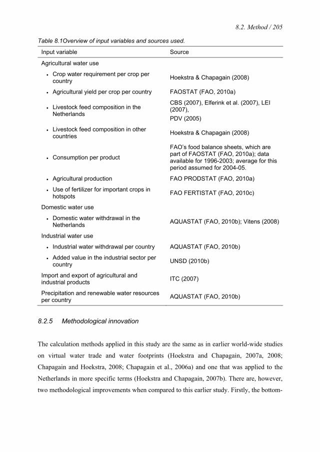
8.2. Method / 205
Table 8.1Overview of input variables and sources used.
Input variable Source
Agricultural water use
• Crop water requirement per crop per country Hoekstra & Chapagain (2008)
• Agricultural yield per crop per country FAOSTAT (FAO, 2010a)
• Livestock feed composition in the Netherlands
CBS (2007), Elferink et al. (2007), LEI (2007), PDV (2005)
• Livestock feed composition in other countries Hoekstra & Chapagain (2008)
• Consumption per product
FAO’s food balance sheets, which are part of FAOSTAT (FAO, 2010a); data available for 1996-2003; average for this period assumed for 2004-05.
• Agricultural production FAO PRODSTAT (FAO, 2010a)
• Use of fertilizer for important crops in hotspots FAO FERTISTAT (FAO, 2010c)
Domestic water use
• Domestic water withdrawal in the Netherlands AQUASTAT (FAO, 2010b); Vitens (2008)
Industrial water use
• Industrial water withdrawal per country AQUASTAT (FAO, 2010b)
• Added value in the industrial sector per country UNSD (2010b)
Import and export of agricultural and industrial products ITC (2007)
Precipitation and renewable water resources per country AQUASTAT (FAO, 2010b)
8.2.5 Methodological innovation
The calculation methods applied in this study are the same as in earlier world-wide studies
on virtual water trade and water footprints (Hoekstra and Chapagain, 2007a, 2008;
Chapagain and Hoekstra, 2008; Chapagain et al., 2006a) and one that was applied to the
Netherlands in more specific terms (Hoekstra and Chapagain, 2007b). There are, however,
two methodological improvements when compared to this earlier study. Firstly, the bottom-
206 / Chapter 8. The external water footprint of the Netherlands
up approach is applied to calculate the water footprint which is more accurate for a country
as the Netherlands, where trade flows are large if compared to domestic production. This
approach has been tested earlier in a pre-study for the Netherlands; see Gerbens-Leenes and
Hoekstra (2007). Secondly the water footprint of consumed and exported goods is
calculated as a weighted average of domestically produced and imported products (the
variable WF*) instead of taking the water footprint of the domestically produced products
or the global average water footprint in the case that there is no domestic production.
Apart from the methodological improvements, there are differences between the
earlier study and the current one in terms of the data used. In the current study we analyze
the ten-year period 1996-2005 instead of a five-year period 1997-2001, which diminishes
the influence of inter-annual differences due to trade flow delays. Besides, more accurate
data in the current study with respect to livestock feed composition are used. Finally, the
current study extends the earlier study by making a first step from water footprint
estimation towards impact assessment by comparing water footprints to water-scarcity
indicators for the identification of hotspots.
8.3 Results
8.3.1 The water footprint of Dutch consumers
The total water footprint of Dutch consumers is about 2300 m3 per capita per year for the
period 1996-2005. Agricultural goods are responsible for the largest part of the footprint
(67%), industrial goods are responsible for 31% and domestic water use accounts for about
2% (Figure 8.2).
The water footprint due to the consumption of agricultural products is specified
further into product categories. Livestock products make up 31% of the water footprint. Oil
crops and oil from oil crops are large contributors as well (12%). The consumption of
coffee, tea, cocoa and tobacco contributes another 8% and cereals and beer, which is made
from barley, contribute 5%. Cotton products and fruit contribute 4% and 3% respectively.
The remainder of the footprint is related to other agricultural products (4%). A more
detailed overview of the individual contribution of product categories to the water footprint
of Dutch consumers is given in Table 8.2. In Table 8.3 the results of both the bottom-up
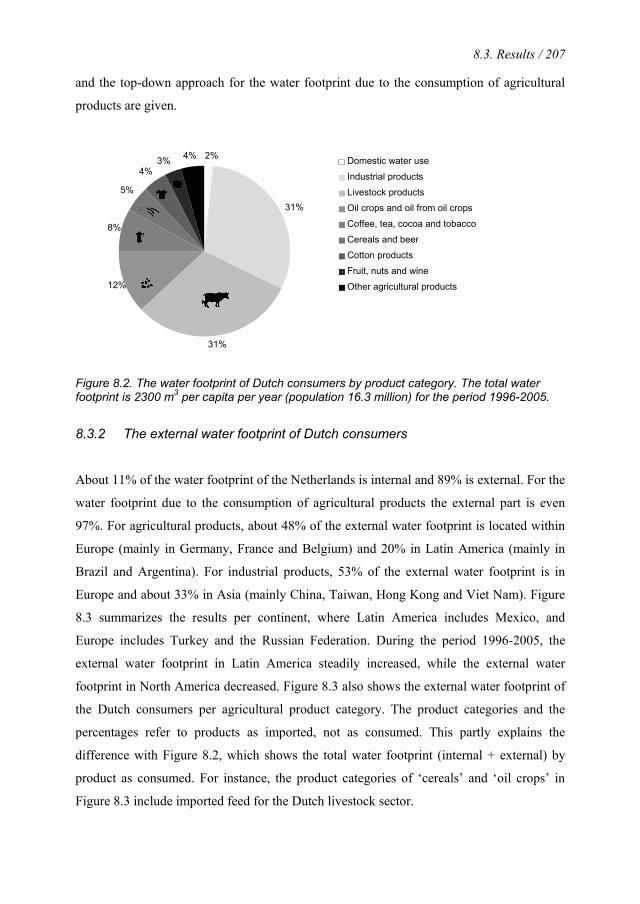
8.3. Results / 207
and the top-down approach for the water footprint due to the consumption of agricultural
products are given.
Figure 8.2. The water footprint of Dutch consumers by product category. The total water footprint is 2300 m3 per capita per year (population 16.3 million) for the period 1996-2005.
8.3.2 The external water footprint of Dutch consumers
About 11% of the water footprint of the Netherlands is internal and 89% is external. For the
water footprint due to the consumption of agricultural products the external part is even
97%. For agricultural products, about 48% of the external water footprint is located within
Europe (mainly in Germany, France and Belgium) and 20% in Latin America (mainly in
Brazil and Argentina). For industrial products, 53% of the external water footprint is in
Europe and about 33% in Asia (mainly China, Taiwan, Hong Kong and Viet Nam). Figure
8.3 summarizes the results per continent, where Latin America includes Mexico, and
Europe includes Turkey and the Russian Federation. During the period 1996-2005, the
external water footprint in Latin America steadily increased, while the external water
footprint in North America decreased. Figure 8.3 also shows the external water footprint of
the Dutch consumers per agricultural product category. The product categories and the
percentages refer to products as imported, not as consumed. This partly explains the
difference with Figure 8.2, which shows the total water footprint (internal + external) by
product as consumed. For instance, the product categories of ‘cereals’ and ‘oil crops’ in
Figure 8.3 include imported feed for the Dutch livestock sector.
5% 4%
3% 4%
8%
12%
31%
31%
2% Domestic water use Industrial products Livestock products Oil crops and oil from oil crops Coffee, tea, cocoa and tobacco Cereals and beer Cotton products Fruit, nuts and wine Other agricultural products
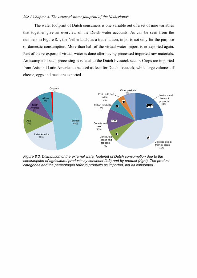
208 / Chapter 8. The external water footprint of the Netherlands
The water footprint of Dutch consumers is one variable out of a set of nine variables
that together give an overview of the Dutch water accounts. As can be seen from the
numbers in Figure 8.1, the Netherlands, as a trade nation, imports not only for the purpose
of domestic consumption. More than half of the virtual water import is re-exported again.
Part of the re-export of virtual-water is done after having processed imported raw materials.
An example of such processing is related to the Dutch livestock sector. Crops are imported
from Asia and Latin America to be used as feed for Dutch livestock, while large volumes of
cheese, eggs and meat are exported.
Europe48%
Latin America20%
Asia14%
North America
9%
Africa8%
Oceania1%
Coffee, tea, cocoa and tobacco
7%
Cereals and beer13%
Cotton products7%
Fruit, nuts and wine4%
Other products7%
Oil crops and oil from oil crops
40%
Livestock and livestock products
22%
Figure 8.3. Distribution of the external water footprint of Dutch consumption due to the consumption of agricultural products by continent (left) and by product (right). The product categories and the percentages refer to products as imported, not as consumed.
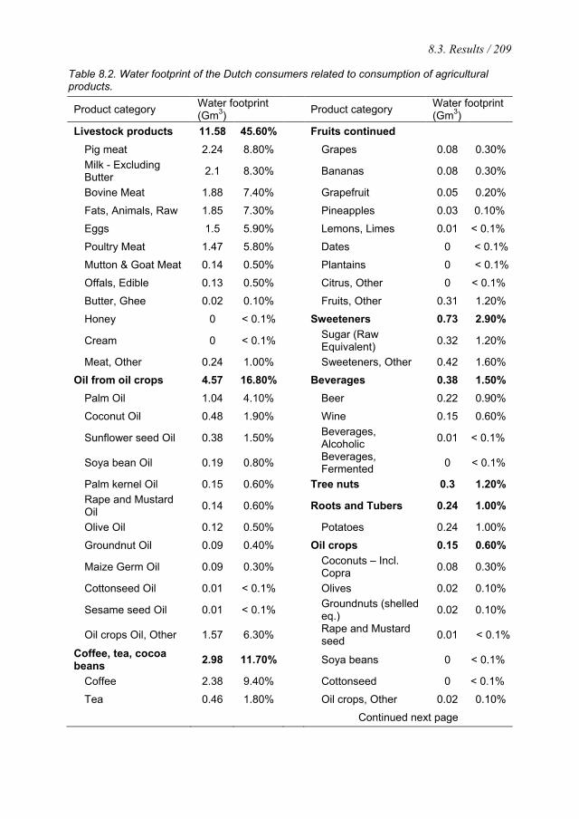
8.3. Results / 209
Table 8.2. Water footprint of the Dutch consumers related to consumption of agricultural products.
Product category Water footprint (Gm3) Product category Water footprint
(Gm3) Livestock products 11.58 45.60% Fruits continued
Pig meat 2.24 8.80% Grapes 0.08 0.30% Milk - Excluding Butter 2.1 8.30% Bananas 0.08 0.30%
Bovine Meat 1.88 7.40% Grapefruit 0.05 0.20%
Fats, Animals, Raw 1.85 7.30% Pineapples 0.03 0.10%
Eggs 1.5 5.90% Lemons, Limes 0.01 < 0.1%
Poultry Meat 1.47 5.80% Dates 0 < 0.1%
Mutton & Goat Meat 0.14 0.50% Plantains 0 < 0.1%
Offals, Edible 0.13 0.50% Citrus, Other 0 < 0.1%
Butter, Ghee 0.02 0.10% Fruits, Other 0.31 1.20%
Honey 0 < 0.1% Sweeteners 0.73 2.90%
Cream 0 < 0.1% Sugar (Raw Equivalent) 0.32 1.20%
Meat, Other 0.24 1.00% Sweeteners, Other 0.42 1.60% Oil from oil crops 4.57 16.80% Beverages 0.38 1.50%
Palm Oil 1.04 4.10% Beer 0.22 0.90%
Coconut Oil 0.48 1.90% Wine 0.15 0.60%
Sunflower seed Oil 0.38 1.50% Beverages, Alcoholic 0.01 < 0.1%
Soya bean Oil 0.19 0.80% Beverages, Fermented 0 < 0.1%
Palm kernel Oil 0.15 0.60% Tree nuts 0.3 1.20% Rape and Mustard Oil 0.14 0.60% Roots and Tubers 0.24 1.00%
Olive Oil 0.12 0.50% Potatoes 0.24 1.00%
Groundnut Oil 0.09 0.40% Oil crops 0.15 0.60%
Maize Germ Oil 0.09 0.30% Coconuts – Incl. Copra 0.08 0.30%
Cottonseed Oil 0.01 < 0.1% Olives 0.02 0.10%
Sesame seed Oil 0.01 < 0.1% Groundnuts (shelled eq.) 0.02 0.10%
Oil crops Oil, Other 1.57 6.30% Rape and Mustard seed 0.01 < 0.1%
Coffee, tea, cocoa beans 2.98 11.70% Soya beans 0 < 0.1%
Coffee 2.38 9.40% Cottonseed 0 < 0.1%
Tea 0.46 1.80% Oil crops, Other 0.02 0.10%
Continued next page
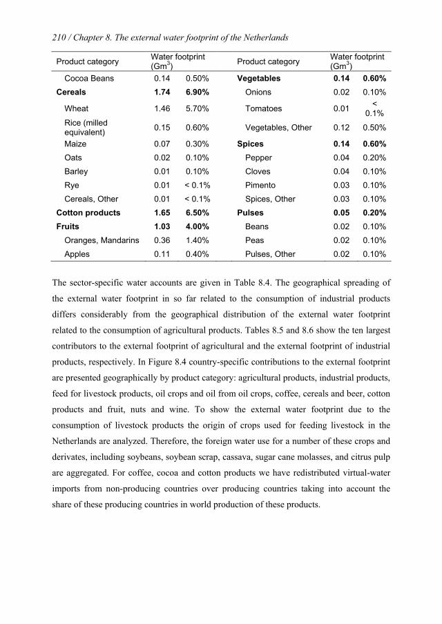
210 / Chapter 8. The external water footprint of the Netherlands
Product category Water footprint (Gm3) Product category Water footprint
(Gm3) Cocoa Beans 0.14 0.50% Vegetables 0.14 0.60%
Cereals 1.74 6.90% Onions 0.02 0.10%
Wheat 1.46 5.70% Tomatoes 0.01 < 0.1%
Rice (milled equivalent) 0.15 0.60% Vegetables, Other 0.12 0.50%
Maize 0.07 0.30% Spices 0.14 0.60% Oats 0.02 0.10% Pepper 0.04 0.20%
Barley 0.01 0.10% Cloves 0.04 0.10%
Rye 0.01 < 0.1% Pimento 0.03 0.10%
Cereals, Other 0.01 < 0.1% Spices, Other 0.03 0.10% Cotton products 1.65 6.50% Pulses 0.05 0.20% Fruits 1.03 4.00% Beans 0.02 0.10%
Oranges, Mandarins 0.36 1.40% Peas 0.02 0.10%
Apples 0.11 0.40% Pulses, Other 0.02 0.10%
The sector-specific water accounts are given in Table 8.4. The geographical spreading of
the external water footprint in so far related to the consumption of industrial products
differs considerably from the geographical distribution of the external water footprint
related to the consumption of agricultural products. Tables 8.5 and 8.6 show the ten largest
contributors to the external footprint of agricultural and the external footprint of industrial
products, respectively. In Figure 8.4 country-specific contributions to the external footprint
are presented geographically by product category: agricultural products, industrial products,
feed for livestock products, oil crops and oil from oil crops, coffee, cereals and beer, cotton
products and fruit, nuts and wine. To show the external water footprint due to the
consumption of livestock products the origin of crops used for feeding livestock in the
Netherlands are analyzed. Therefore, the foreign water use for a number of these crops and
derivates, including soybeans, soybean scrap, cassava, sugar cane molasses, and citrus pulp
are aggregated. For coffee, cocoa and cotton products we have redistributed virtual-water
imports from non-producing countries over producing countries taking into account the
share of these producing countries in world production of these products.
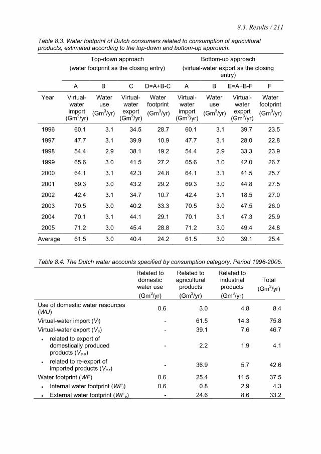
8.3. Results / 211
Table 8.3. Water footprint of Dutch consumers related to consumption of agricultural products, estimated according to the top-down and bottom-up approach.
Top-down approach (water footprint as the closing entry)
Bottom-up approach (virtual-water export as the closing
entry)
A B C D=A+B-C A B E=A+B-F F
Year Virtual-water import
(Gm3/yr)
Water use
(Gm3/yr)
Virtual-water export
(Gm3/yr)
Water footprint (Gm3/yr)
Virtual-water import
(Gm3/yr)
Water use
(Gm3/yr)
Virtual-water export
(Gm3/yr)
Water footprint (Gm3/yr)
1996 60.1 3.1 34.5 28.7 60.1 3.1 39.7 23.5
1997 47.7 3.1 39.9 10.9 47.7 3.1 28.0 22.8
1998 54.4 2.9 38.1 19.2 54.4 2.9 33.3 23.9
1999 65.6 3.0 41.5 27.2 65.6 3.0 42.0 26.7
2000 64.1 3.1 42.3 24.8 64.1 3.1 41.5 25.7
2001 69.3 3.0 43.2 29.2 69.3 3.0 44.8 27.5
2002 42.4 3.1 34.7 10.7 42.4 3.1 18.5 27.0
2003 70.5 3.0 40.2 33.3 70.5 3.0 47.5 26.0
2004 70.1 3.1 44.1 29.1 70.1 3.1 47.3 25.9
2005 71.2 3.0 45.4 28.8 71.2 3.0 49.4 24.8
Average 61.5 3.0 40.4 24.2 61.5 3.0 39.1 25.4
Table 8.4. The Dutch water accounts specified by consumption category. Period 1996-2005.
Related to domestic water use
(Gm3/yr)
Related to agricultural products (Gm3/yr)
Related to industrial products (Gm3/yr)
Total (Gm3/yr)
Use of domestic water resources (WU) 0.6 3.0 4.8 8.4
Virtual-water import (Vi) - 61.5 14.3 75.8 Virtual-water export (Ve) - 39.1 7.6 46.7 • related to export of
domestically produced products (Ve,d)
- 2.2 1.9 4.1
• related to re-export of imported products (Ve,r)
- 36.9 5.7 42.6
Water footprint (WF) 0.6 25.4 11.5 37.5 • Internal water footprint (WFi) 0.6 0.8 2.9 4.3 • External water footprint (WFe) - 24.6 8.6 33.2
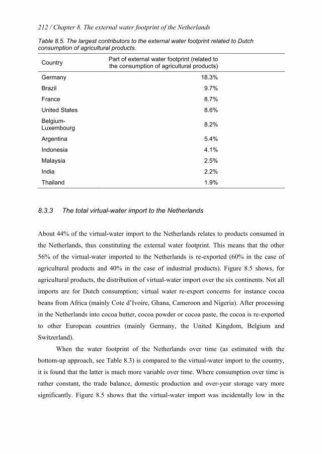
212 / Chapter 8. The external water footprint of the Netherlands
Table 8.5. The largest contributors to the external water footprint related to Dutch consumption of agricultural products.
Country Part of external water footprint (related to the consumption of agricultural products)
Germany 18.3%
Brazil 9.7%
France 8.7%
United States 8.6%
Belgium-Luxembourg 8.2%
Argentina 5.4%
Indonesia 4.1%
Malaysia 2.5%
India 2.2%
Thailand 1.9%
8.3.3 The total virtual-water import to the Netherlands
About 44% of the virtual-water import to the Netherlands relates to products consumed in
the Netherlands, thus constituting the external water footprint. This means that the other
56% of the virtual-water imported to the Netherlands is re-exported (60% in the case of
agricultural products and 40% in the case of industrial products). Figure 8.5 shows, for
agricultural products, the distribution of virtual-water import over the six continents. Not all
imports are for Dutch consumption; virtual water re-export concerns for instance cocoa
beans from Africa (mainly Cote d’Ivoire, Ghana, Cameroon and Nigeria). After processing
in the Netherlands into cocoa butter, cocoa powder or cocoa paste, the cocoa is re-exported
to other European countries (mainly Germany, the United Kingdom, Belgium and
Switzerland).
When the water footprint of the Netherlands over time (as estimated with the
bottom-up approach, see Table 8.3) is compared to the virtual-water import to the country,
it is found that the latter is much more variable over time. Where consumption over time is
rather constant, the trade balance, domestic production and over-year storage vary more
significantly. Figure 8.5 shows that the virtual-water import was incidentally low in the
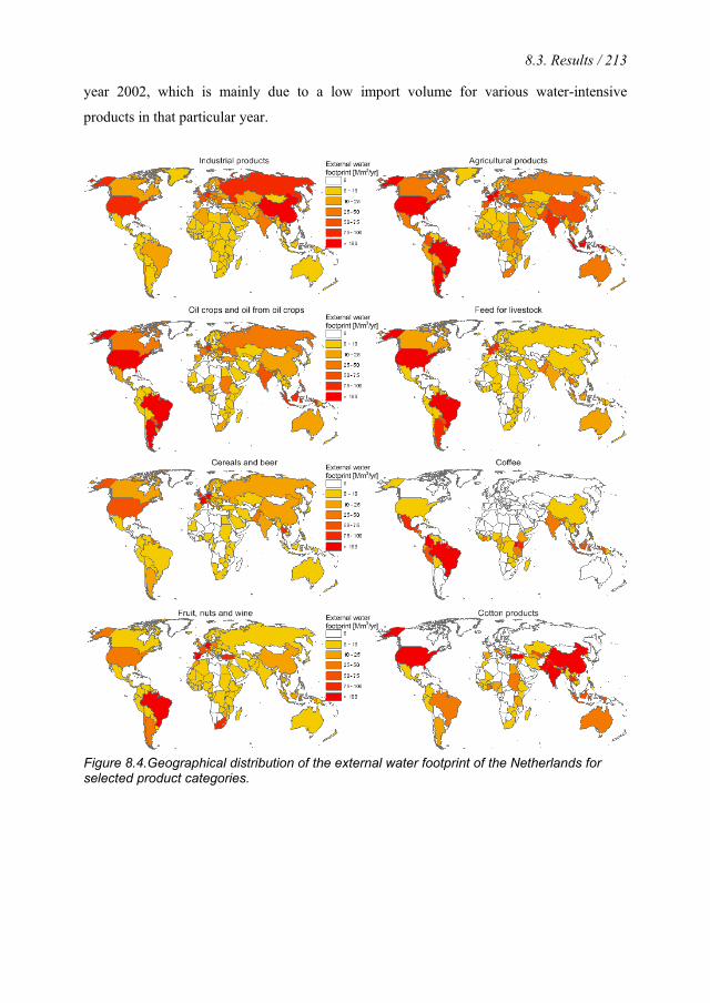
8.3. Results / 213
year 2002, which is mainly due to a low import volume for various water-intensive
products in that particular year.
Figure 8.4.Geographical distribution of the external water footprint of the Netherlands for selected product categories.
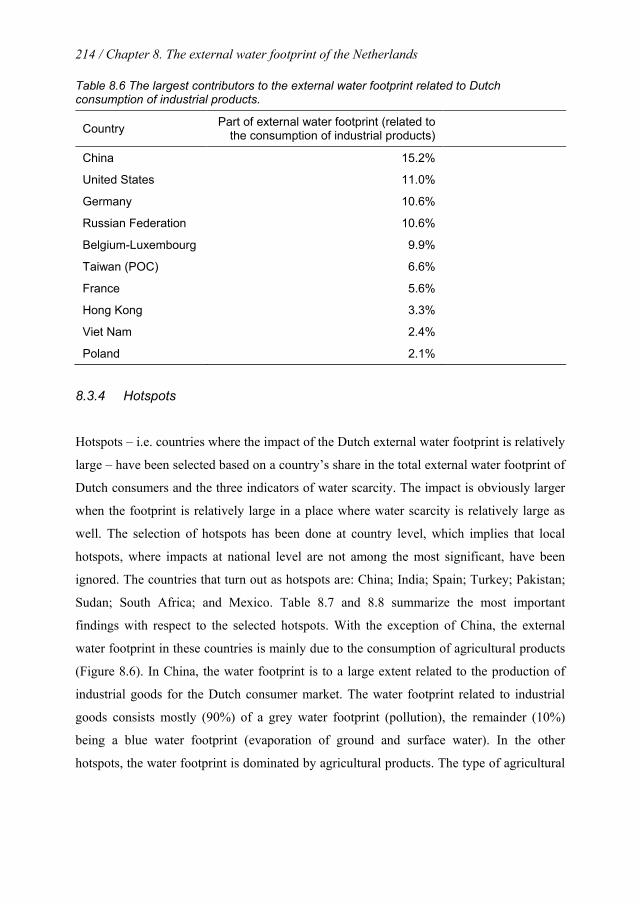
214 / Chapter 8. The external water footprint of the Netherlands
Table 8.6 The largest contributors to the external water footprint related to Dutch consumption of industrial products.
Country Part of external water footprint (related to the consumption of industrial products)
China 15.2%
United States 11.0%
Germany 10.6%
Russian Federation 10.6%
Belgium-Luxembourg 9.9%
Taiwan (POC) 6.6%
France 5.6%
Hong Kong 3.3%
Viet Nam 2.4%
Poland 2.1%
8.3.4 Hotspots
Hotspots – i.e. countries where the impact of the Dutch external water footprint is relatively
large – have been selected based on a country’s share in the total external water footprint of
Dutch consumers and the three indicators of water scarcity. The impact is obviously larger
when the footprint is relatively large in a place where water scarcity is relatively large as
well. The selection of hotspots has been done at country level, which implies that local
hotspots, where impacts at national level are not among the most significant, have been
ignored. The countries that turn out as hotspots are: China; India; Spain; Turkey; Pakistan;
Sudan; South Africa; and Mexico. Table 8.7 and 8.8 summarize the most important
findings with respect to the selected hotspots. With the exception of China, the external
water footprint in these countries is mainly due to the consumption of agricultural products
(Figure 8.6). In China, the water footprint is to a large extent related to the production of
industrial goods for the Dutch consumer market. The water footprint related to industrial
goods consists mostly (90%) of a grey water footprint (pollution), the remainder (10%)
being a blue water footprint (evaporation of ground and surface water). In the other
hotspots, the water footprint is dominated by agricultural products. The type of agricultural
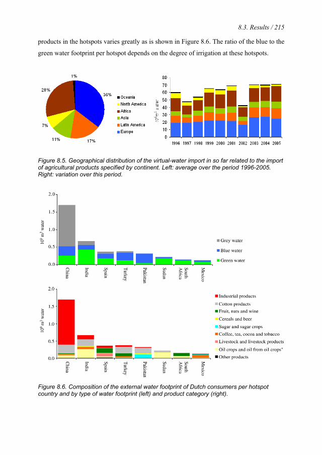
8.3. Results / 215
products in the hotspots varies greatly as is shown in Figure 8.6. The ratio of the blue to the
green water footprint per hotspot depends on the degree of irrigation at these hotspots.
Figure 8.5. Geographical distribution of the virtual-water import in so far related to the import of agricultural products specified by continent. Left: average over the period 1996-2005. Right: variation over this period.
Figure 8.6. Composition of the external water footprint of Dutch consumers per hotspot country and by type of water footprint (left) and product category (right).
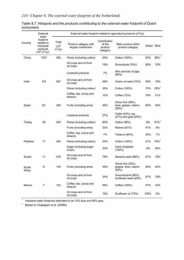
216 / Chapter 8. The external water footprint of the Netherlands
Table 8.7. Hotspots and the products contributing to the external water footprint of Dutch consumers.
Country
External water
footprint related to industrial products
(106 m3/yr) *
External water footprint related to agricultural products (m3/yr)
Total (106
m3/yr)
Product category with largest contribution
Contribution of the
product category
Main product within product category Green Blue
China 1307 393 Fibres (including cotton) 65% Cotton (100%) 62% 38%**
Oil crops and oil from oil crops 16% Groundnuts (74%) 90% 10%
Livestock products 7% Skin and hair of pigs (90%)
India 123 547 Oil crops and oil from oil crops 46% Castor oil seed (72%) 82% 18%
Fibres (including cotton) 35% Cotton (100%) 75% 25%**
Coffee, tea, cocoa and tobacco 10% Coffee (72%) 79% 21%
Spain 63 305 Fruits (including wine) 46% Citrus fruit (36%), wine, grapes, raisins (28%)
60% 40%
Livestock products 27% Cattle (42%), pig (27%) and goat (20%)
Turkey 39 340 Fibres (including cotton) 60% Cotton (99%) 9% 91%**
Fruits (including wine) 23% Raisins (81%) 91% 9%
Coffee, tea, cocoa and tobacco 7% Tobacco (84%) 93% 7%
Pakistan 17 305 Fibres (including cotton) 54% Cotton (100%) 21% 79%**
Sugar (including sugar crops) 33% Cane molasses
(100%) 8% 92%
Sudan <1 218 Oil crops and oil from oil crops 79% Sesame seed (89%) 81% 19%
South Africa
6 145 Fruits (including wine) 49% Citrus fruit (35%), grapes, wine, raisins (29%)
80% 20%
Oil crops and oil from oil crops 34% Groundnut/oil (56%),
sunflower seed (40%) 81% 19%
Mexico 7 123 Coffee, tea, cocoa and tobacco 66% Coffee (100%) 57% 43%
Oil crops and oil from oil crops 16% Sunflower oil (75%) 100% 0%
* Industrial water footprints estimated to be 10% blue and 90% grey. ** Based on Chapagain et al. (2006b).

8.4. Conclusion / 217
Table 8.8. Estimated grey water footprint for specific crops at the hotspots.
Area (km2)*
Area with
fertilizer (%)*
Rate N (kg/ha) *
Rate P (kg/ha) *
Rate K (kg/ha) *
Grey water
footprint (m3/ha)**
China, Mainland (1997)
Cotton 5528 100 120 70 25 1200
Oil crops 668 95 65 40 30 618
India (2003/2004)
Cotton 8500 6 90 23 5 54 Other crops 60400 22 35 19 7 77
Spain (1999/2000) Fruits 4975 n.a. 57 24 26 n.a.
Turkey (1999) Cotton 718 99 127 39 4 1257 Fruits 1240 70 < 0.1 < 0.1 < 0.1 0.4 Tobacco 289 68 3 1 6 20 Pakistan (2001/2002)
Cotton n.a. n.a. 120 50 0.1 n.a. Sugar cane n.a. n.a. 125 56 0.3 n.a.
Sudan* n.a. n.a. n.a. n.a. n.a. n.a. South Africa (2004)
Citrus fruits 64 100 80 35 60 800
Sunflower 640 85 15 21 2 128 Mexico (1998) Coffee 679 60 60 40 15 360
Sunflower 123 80 75 10 0 600 * Source: FAO (2010c). For Sudan, no data on fertiliser use are available. ** Assumptions: nitrogen is the critical factor; 10% of the nitrogen leaches to the water
system; nitrogen water standard 10 mg/litre (Hoekstra and Chapagain, 2008). 8.4 Conclusion
The total water footprint of the Netherlands is estimated to be about 2300 m3/yr/cap, which
is nearly double the water footprint of an average world citizen. About 67% of the Dutch
water footprint relates to the consumption of agricultural goods, 31% to the consumption of
industrial goods, and 2% to domestic water use. The Dutch water footprint related to the
consumption of agricultural goods, is composed as follows: 46% related to livestock
products; 17% oil crops and oil from oil crops; 12% coffee, tea, cocoa and tobacco; 8%
cereals and beer; 6 % cotton products; 5% fruits; and 6 % other agricultural products. Most
agricultural products are related to food consumption, most important exceptions being
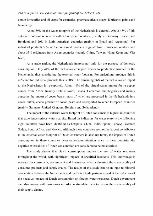
218 / Chapter 8. The external water footprint of the Netherlands
cotton for textiles and oil crops for cosmetics, pharmaceuticals, soaps, lubricants, paints and
bio-energy.
About 89% of the water footprint of the Netherlands is external. About 48% of this
external footprint is located within European countries (mainly in Germany, France and
Belgium) and 20% in Latin American countries (mainly in Brazil and Argentina). For
industrial products 53% of the consumed products originate from European countries and
about 33% originates from Asian countries (mainly China, Taiwan, Hong Kong and Viet
Nam).
As a trade nation, the Netherlands imports not only for the purpose of domestic
consumption. Only 44% of the virtual-water import relates to products consumed in the
Netherlands, thus constituting the external water footprint. For agricultural products this is
40% and for industrial products this is 60%. The remaining 56% of the virtual-water import
to the Netherlands is re-exported. About 41% of the virtual-water import for re-export
comes from Africa (mainly Cote d’Ivoire, Ghana, Cameroon and Nigeria) and mainly
concerns the import of cocoa beans, most of which are processed in the Netherlands into
cocoa butter, cocoa powder or cocoa paste and re-exported to other European countries
(mainly Germany, United Kingdom, Belgium and Switzerland).
The impact of the external water footprint of Dutch consumers is highest in countries
that experience serious water scarcity. Based on indicators for water scarcity the following
eight countries have been identified as hotspots: China; India; Spain; Turkey; Pakistan;
Sudan; South Africa; and Mexico. Although these countries are not the largest contributors
to the external water footprint of Dutch consumers in absolute terms, the impact of Dutch
consumption in these countries deserves serious attention since in these countries the
negative externalities of Dutch consumption are considered to be most serious.
The study shows that Dutch consumption implies the use of water resources
throughout the world, with significant impacts at specified locations. This knowledge is
relevant for consumers, government and businesses when addressing the sustainability of
consumer products and supply chains. The results of this study can be an input to bilateral
cooperation between the Netherlands and the Dutch trade partners aimed at the reduction of
the negative impacts of Dutch consumption on foreign water resources. Dutch government
can also engage with businesses in order to stimulate them to review the sustainability of
their supply chains.
9. The relation between national water management and international trade: A case study for Kenya11
Abstract This study estimates the water footprint of Kenya both from the production and
consumption perspective and estimates virtual water import and export flows related to
international trade. Both the water footprint and virtual water estimates are broken down
into three components: green, blue and grey water. The main findings of the study are:
• During the period 1996-2005, the water footprint of Kenya related to crop
production was 18.1 Gm3/yr.
• During the same period, Kenya’s virtual water import and export were 3.96
Gm3/yr and 4.1 Gm3/yr respectively. Over 78% of the virtual water export was
related to export of coffee, tea and cotton products. The water use in Kenya for
producing flowers for export was 20 Mm3/yr.
• The average export earnings per unit of water consumed or polluted for producing
agricultural export products was US$ 0.25 per cubic metre of water; the average
cost of imported commodities per unit of virtual water imported was 0.10 US$/m3.
• About 23% of the water appropriated in the agricultural sector in Kenya is for
producing export products, amongst which coffee, tea, cotton, fruits, vegetables
and flowers. On the other hand, it imports many other water-intensive goods,
primarily cereals and oil crops. As a result of the latter, Kenya is not self-sufficient
with respect to its own food supply: 10% of its maize (the major staple food), 63%
of its wheat and 72% of its rice are imported.
• The total water footprint related to consumption of both agricultural and industrial
goods and domestic water use was 35 Gm3/yr, which is 1100 m3/yr per capita on
average (79% of the global average).
11 Based on Mekonnen and Hoekstra (2011d)

220 / Chapter 9. National water management: A case study for Kenya
Kenya could address its water scarcity problem through enhancing its import of water-
intensive products such as cereals and export of non water-intensive and high value
products such as cut flower and tea. From a water resources point of view, particularly the
production and export of green-water based tea and vegetables are positive: water
productivities in terms of US$ per cubic metre are relatively high and the export values in
absolute terms are very substantial.
9.1 Introduction
There are great disparities in water use and scarcity within and between countries because
both people and water resources are unevenly distributed across the globe. Virtual water
import in the form of import of agricultural goods is increasingly recognized as a
mechanism to improve national water security (Allan, 2003; De Fraiture et al., 2004;
Hoekstra, 2003; Chapagain et al., 2006a; Yang et al., 2006; Hoekstra and Chapagain,
2008). Virtual water import enables nations to save scarce domestic water resources by
importing water-intensive products and exporting commodities that require little water. On
the other hand, water-abundant countries can profit by exporting water-intensive
commodities (Hoekstra and Chapagain, 2008).
Kenya’s internal renewable water resources are estimated at 20.7 Gm3/yr. Most of
this, 20.2 Gm3/yr, is available as surface water. Renewable ground water resources are
estimates to be 3.5 Gm3/yr, of which 3.0 Gm3/yr overlaps with the annual renewable
surface water resources. It is estimated that 10 Gm3/yr of river water flows into the country
(FAO, 2005c), which means that the total renewable water resources of Kenya are 30.7
Gm3/yr.
According to Wong et al. (2005), the available renewable water resources are
insufficient to meet Kenya’s water needs. Kenya is generally characterized as a water-
stressed country (Ohlsson and Appelgren, 1998; FAO, 2005c; UNEP, 2006). This is also
the starting point of Kenya’s Vision 2030 document (GoK, 2007).
The aim of this paper is to assess the relation between national water management
and international trade in a case study for Kenya. We quantify the water consumption and
pollution related to the production of agricultural export commodities and put this in the
9.2. Method and data / 221
context of export earnings. We also consider the import side by quantifying how much
water is embedded in imported commodities.
9.2 Method and data
The water footprint is an indicator of human appropriation of freshwater resources. The
term ‘freshwater appropriation’ refers to both consumptive water use (water evaporated or
incorporated into the product) and water required to assimilate pollutants. The water
footprint has three colour coded components: the green, blue and grey water footprint. The
green water footprint is the volume of green water (rainwater) consumed. The blue water
footprint refers to consumption of blue water resources (surface and ground water). The
grey water footprint is an indicator of the degree of freshwater pollution and is defined as
the volume of freshwater that is required to assimilate the load of pollutants based on
existing ambient water quality standards.
Green, blue and grey water footprints have been estimated following the calculation
framework as set out in The Water Footprint Assessment Manual developed by the Water
Footprint Network (Hoekstra et al., 2011). The water footprint within a nation is defined as
the total freshwater volume consumed or polluted within the territory of the nation as a
result of different economic activities. The water footprint of national consumption refers to
the total amount of fresh water that is used to produce the goods and services consumed by
the inhabitants of the nation. It includes both an internal and an external component. The
external water footprint of national consumption is related to the fact that water is
consumed or polluted elsewhere to produce commodities imported by Kenya.
The water footprint within a nation is defined as the total freshwater volume
consumed or polluted within the territory of the nation as a result of different economic
activities. The water footprint related to agricultural production including both crop
production and farm animal production were taken from Mekonnen and Hoekstra (2010d,e,
2011a). The water footprints within Kenya related to industrial production and domestic
water supply were taken from Mekonnen and Hoekstra (2011b).
The virtual-water export from a nation is the sum of virtual water export from
domestic water resources and re-exported virtual water of foreign origin. The gross virtual-
water flow is calculated by multiplying the volume of trade by the water footprint per ton of

222 / Chapter 9. National water management: A case study for Kenya
product as in the exporting nation. We have taken the average product water footprint as in
the exporting country and when a product is imported from a country that does not produce
the product we have assumed the global average product water footprint for that import
flow. Kenya’s virtual water import and export related to trade in industrial products was
taken from Mekonnen and Hoekstra (2011b).
The water footprint of national consumption is defined as the total volume of
freshwater that is used to produce the goods and services consumed by the inhabitant of the
nation. The water footprint of the national consumption can be distinguished between the
internal water footprint and the external water footprint. The internal water footprint of
national consumption refers to the use of domestic water resources to produce goods and
services consumed by the national population. It is the difference between the water
footprint within the nation and the volume of virtual-water export to other nations related to
export of products produced with domestic water resources. The external water footprint of
national consumption, on the other hand, is defined as the volume of water resources used
in other nations to produce goods and services consumed by the population in the nation
considered. It is the difference between the virtual-water import into the nation and the
volume of virtual-water re-exported to other nations as a result of re-export of imported
products.
The water footprint of national consumption is calculated by adding the direct and
indirect water footprint of consumers within the nation. The direct water footprint of
consumers within the nation refers to consumption and pollution of water related to
domestic water supply. The indirect water footprint of consumers refers to the water use by
others to make the commodities consumed, whereby we distinguish between agricultural
and industrial commodities. The water footprint of national consumption of agricultural and
industrial commodities can be calculated through either the top-down or the bottom-up
approach (Hoekstra et al., 2011). In the top-down approach, the water footprint of national
consumption is calculated as the water footprint within the nation plus the virtual-water
import minus the virtual-water export. In the bottom-up approach, the water footprint of
national consumption is calculated by adding the direct and indirect water footprints of
consumers within the nation. The water footprint of national consumption was taken from
Mekonnen and Hoekstra (2011b).

9.3. Results / 223
The water productivity of crops was calculated by dividing the total value of crop and the
total water footprint related to crop production. The total value of crops was derived based
on the unit value of exported products and total production of the product considered. Data
on export and import value of agricultural products have been taken from the SITA
database (Statistics for International Trade Analysis) available from the International Trade
Centre (ITC, 2007).
9.3 Results
9.3.1 Water footprint of crop production
The water footprint related to crop production in Kenya for the period 1996-2005 was 18.1
Gm3/yr (97% green, 1% blue and 2% grey). The largest share of this water footprint is due
to the production of maize, which accounts for about 38% of the total production water
footprint. Dry beans, coffee, tea and wheat together account 33% toward the total
production water footprint (Table 9.1).
About 61% of the total green water footprint is due to the production of maize (6.8
Gm3/yr), dry beans (2.8 Gm3/yr) and coffee (1.5 Gm3/yr). The largest production blue water
footprint was estimated for growing coffee (51 Mm3/yr) and rice (35 Mm3/yr), which
together account for 40% of the total blue water footprint related to crop production.
Although the fertilizer application rates are still very low by international standards,
Kenya has among the highest fertilizer application rates within Sub-Saharan African
countries, excluding South Africa. Fertilizer use has grown on average by more than 30%
over the last few years and in 2004/05 total consumption reached over 350 thousand metric
tonnes (Ariga et. al., 2006). Not all fertilizer applied will be absorbed by the plant. A
significant amount of nitrogen can remain in the soil and some of this will eventually leach
into ground and surface water, causing water pollution. In this study, we have estimated the
total volume of water required to dilute the polluted water (the grey water footprint) due to
nitrogen fertilizer leaching from crop fields. For the period 1996-2005, the total grey water
footprint related to the production of crops was 300 Mm3/yr. A little over half of the grey
water footprint is related production of three crops - maize, coffee, and potato. About 23%
of the agricultural water footprint was used for producing export products. The remaining
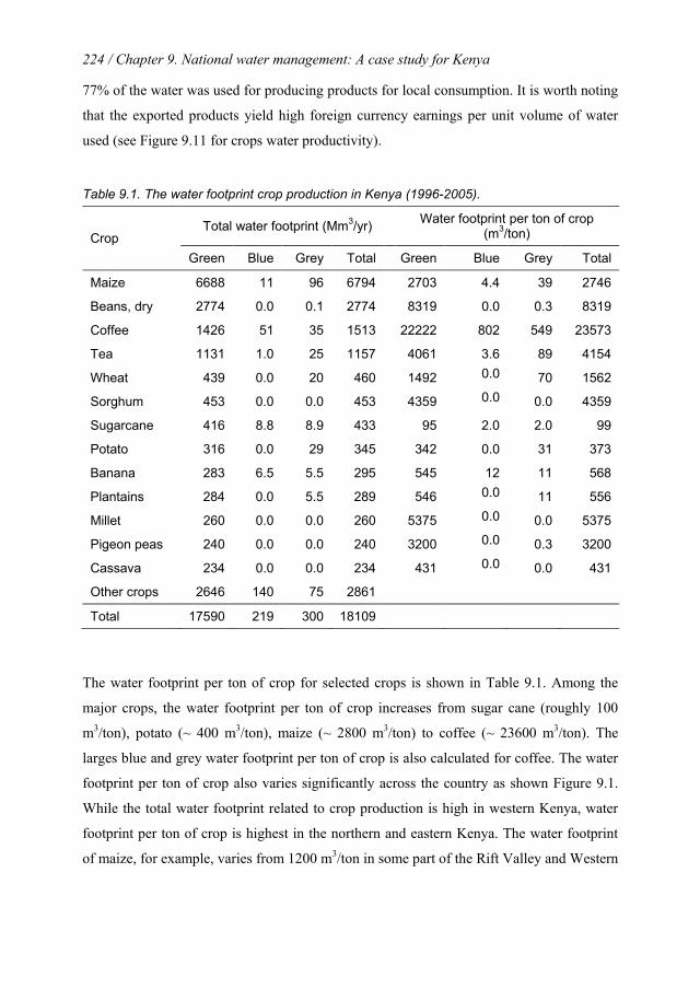
224 / Chapter 9. National water management: A case study for Kenya
77% of the water was used for producing products for local consumption. It is worth noting
that the exported products yield high foreign currency earnings per unit volume of water
used (see Figure 9.11 for crops water productivity).
Table 9.1. The water footprint crop production in Kenya (1996-2005).
Crop Total water footprint (Mm3/yr) Water footprint per ton of crop
(m3/ton)
Green Blue Grey Total Green Blue Grey Total
Maize 6688 11 96 6794 2703 4.4 39 2746
Beans, dry 2774 0.0 0.1 2774 8319 0.0 0.3 8319
Coffee 1426 51 35 1513 22222 802 549 23573
Tea 1131 1.0 25 1157 4061 3.6 89 4154
Wheat 439 0.0 20 460 1492 0.0 70 1562
Sorghum 453 0.0 0.0 453 4359 0.0 0.0 4359
Sugarcane 416 8.8 8.9 433 95 2.0 2.0 99
Potato 316 0.0 29 345 342 0.0 31 373
Banana 283 6.5 5.5 295 545 12 11 568
Plantains 284 0.0 5.5 289 546 0.0 11 556
Millet 260 0.0 0.0 260 5375 0.0 0.0 5375
Pigeon peas 240 0.0 0.0 240 3200 0.0 0.3 3200
Cassava 234 0.0 0.0 234 431 0.0 0.0 431
Other crops 2646 140 75 2861
Total 17590 219 300 18109
The water footprint per ton of crop for selected crops is shown in Table 9.1. Among the
major crops, the water footprint per ton of crop increases from sugar cane (roughly 100
m3/ton), potato (~ 400 m3/ton), maize (~ 2800 m3/ton) to coffee (~ 23600 m3/ton). The
larges blue and grey water footprint per ton of crop is also calculated for coffee. The water
footprint per ton of crop also varies significantly across the country as shown Figure 9.1.
While the total water footprint related to crop production is high in western Kenya, water
footprint per ton of crop is highest in the northern and eastern Kenya. The water footprint
of maize, for example, varies from 1200 m3/ton in some part of the Rift Valley and Western
9.3. Results / 225
provinces to as high as 6000 m3/ton in the Eastern province (Figure 9.1). The reason for this
difference in water footprint per unit of product between the provinces is due mainly to
difference in the climatic condition. The northern and eastern regions of Kenya are arid or
semi-arid with annual precipitation as low as 200 mm which affects crop yield negatively.
The total water footprint of crop production for each province of Kenya is shown in
Figure 9.2. The Rift Valley province accounts for about 39% of the total water footprint
related to crop production. The larges blue water footprint is found in Rift Valley (25%)
and Nyanza (20%) provinces. Rift Valley province alone accounts for 35% of the grey
water footprint. Since most of Kenya’s farming system relies heavily on rainfall, the
croplands are mainly concentrated in places where rainfall is more reliable, such as the
highlands, the Lake Victoria basin, and the narrow coastal strip. The green water footprint
dominates (>95%) in all provinces reaching up to 98% in Rift Valley and Western
provinces (Figure 9.2). The variation in the total water footprint per grid cell (Figure 9.3)
shows similar pattern as the fraction of harvested crop area (Monfreda et al., 2008). This
indicates that total water footprint per grid cell is largely determined by the fraction of
harvested crop area per grid cell.
9.3.2 Virtual water flow related to trade in agricultural products
In the period 1996-2005, Kenya’s virtual water export related to agricultural products was
4.1 Gm3/yr (95% green, 3% blue and 2% grey). About 65% was related to export of coffee
and tea. Cotton products, livestock products and products of oil crops are the other
agricultural products responsible for significant virtual water export from Kenya as shown
in Table 9.2. Kenya’s total export earnings was US$ 1.02 billion. As shown in Table 9.2,
cut flowers generate the highest economic returns per unit of water exported, followed by
vegetable products. The major destinations for Kenya’s virtual water exports are the US,
Germany, the UK, and Pakistan, which together account for about 45% of Kenya’s virtual
water exports.

226 / Chapter 9. National water management: A case study for Kenya
Figure 9.1. The green, blue and grey water footprints per ton of maize (top) and coffee (bottom). Period 1996-2005
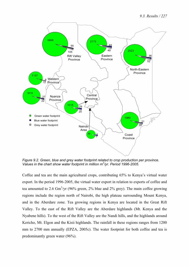
9.3. Results / 227
Nairobi Area
Central Province
Coast Province
North-Eastern Province
Eastern Province
Rift Valley Province
Nyanza Province
Western Province
217544
49
181527
22
2523
36
52
11576
12
1015 29
20
50 21
198921
39Grey water footprint
Blue water footprint
Green water footprint
6868
55
105
Figure 9.2. Green, blue and grey water footprint related to crop production per province. Values in the chart show water footprint in million m3/yr. Period 1996-2005.
Coffee and tea are the main agricultural crops, contributing 65% to Kenya’s virtual water
export. In the period 1996-2005, the virtual water export in relation to exports of coffee and
tea amounted to 2.6 Gm3/yr (96% green, 2% blue and 2% grey). The main coffee growing
regions include the region north of Nairobi, the high plateau surrounding Mount Kenya,
and in the Aberdare zone. Tea growing regions in Kenya are located in the Great Rift
Valley. To the east of the Rift Valley are the Aberdare highlands (Mt. Kenya and the
Nyabene hills). To the west of the Rift Valley are the Nandi hills, and the highlands around
Kericho, Mt. Elgon and the Kisii highlands. The rainfall in these regions ranges from 1200
mm to 2700 mm annually (EPZA, 2005c). The water footprint for both coffee and tea is
predominantly green water (96%).
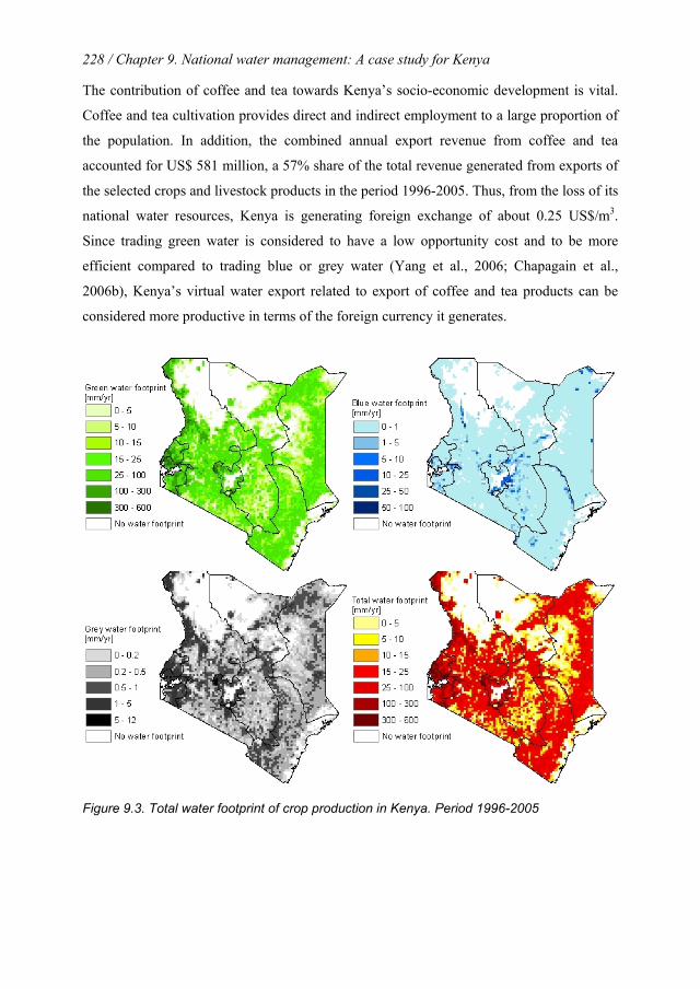
228 / Chapter 9. National water management: A case study for Kenya
The contribution of coffee and tea towards Kenya’s socio-economic development is vital.
Coffee and tea cultivation provides direct and indirect employment to a large proportion of
the population. In addition, the combined annual export revenue from coffee and tea
accounted for US$ 581 million, a 57% share of the total revenue generated from exports of
the selected crops and livestock products in the period 1996-2005. Thus, from the loss of its
national water resources, Kenya is generating foreign exchange of about 0.25 US$/m3.
Since trading green water is considered to have a low opportunity cost and to be more
efficient compared to trading blue or grey water (Yang et al., 2006; Chapagain et al.,
2006b), Kenya’s virtual water export related to export of coffee and tea products can be
considered more productive in terms of the foreign currency it generates.
Figure 9.3. Total water footprint of crop production in Kenya. Period 1996-2005
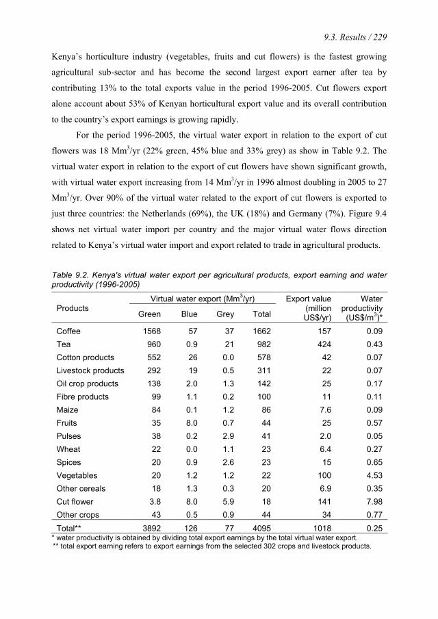
9.3. Results / 229
Kenya’s horticulture industry (vegetables, fruits and cut flowers) is the fastest growing
agricultural sub-sector and has become the second largest export earner after tea by
contributing 13% to the total exports value in the period 1996-2005. Cut flowers export
alone account about 53% of Kenyan horticultural export value and its overall contribution
to the country’s export earnings is growing rapidly.
For the period 1996-2005, the virtual water export in relation to the export of cut
flowers was 18 Mm3/yr (22% green, 45% blue and 33% grey) as show in Table 9.2. The
virtual water export in relation to the export of cut flowers have shown significant growth,
with virtual water export increasing from 14 Mm3/yr in 1996 almost doubling in 2005 to 27
Mm3/yr. Over 90% of the virtual water related to the export of cut flowers is exported to
just three countries: the Netherlands (69%), the UK (18%) and Germany (7%). Figure 9.4
shows net virtual water import per country and the major virtual water flows direction
related to Kenya’s virtual water import and export related to trade in agricultural products.
Table 9.2. Kenya's virtual water export per agricultural products, export earning and water productivity (1996-2005)
Products Virtual water export (Mm3/yr) Export value
(million US$/yr)
Water productivity
(US$/m3)* Green Blue Grey Total
Coffee 1568 57 37 1662 157 0.09 Tea 960 0.9 21 982 424 0.43 Cotton products 552 26 0.0 578 42 0.07 Livestock products 292 19 0.5 311 22 0.07 Oil crop products 138 2.0 1.3 142 25 0.17 Fibre products 99 1.1 0.2 100 11 0.11 Maize 84 0.1 1.2 86 7.6 0.09 Fruits 35 8.0 0.7 44 25 0.57 Pulses 38 0.2 2.9 41 2.0 0.05 Wheat 22 0.0 1.1 23 6.4 0.27 Spices 20 0.9 2.6 23 15 0.65 Vegetables 20 1.2 1.2 22 100 4.53 Other cereals 18 1.3 0.3 20 6.9 0.35 Cut flower 3.8 8.0 5.9 18 141 7.98 Other crops 43 0.5 0.9 44 34 0.77 Total** 3892 126 77 4095 1018 0.25
* water productivity is obtained by dividing total export earnings by the total virtual water export. ** total export earning refers to export earnings from the selected 302 crops and livestock products.
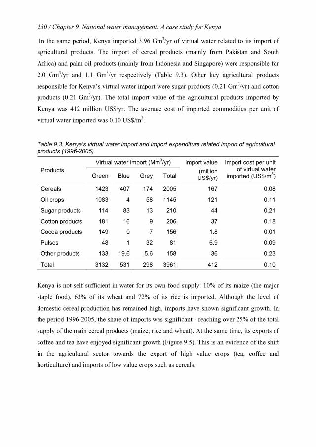
230 / Chapter 9. National water management: A case study for Kenya
In the same period, Kenya imported 3.96 Gm3/yr of virtual water related to its import of
agricultural products. The import of cereal products (mainly from Pakistan and South
Africa) and palm oil products (mainly from Indonesia and Singapore) were responsible for
2.0 Gm3/yr and 1.1 Gm3/yr respectively (Table 9.3). Other key agricultural products
responsible for Kenya’s virtual water import were sugar products (0.21 Gm3/yr) and cotton
products (0.21 Gm3/yr). The total import value of the agricultural products imported by
Kenya was 412 million US$/yr. The average cost of imported commodities per unit of
virtual water imported was 0.10 US$/m3.
Table 9.3. Kenya's virtual water import and import expenditure related import of agricultural products (1996-2005)
Products Virtual water import (Mm3/yr) Import value
(million US$/yr)
Import cost per unit of virtual water
imported (US$/m3) Green Blue Grey Total
Cereals 1423 407 174 2005 167 0.08
Oil crops 1083 4 58 1145 121 0.11
Sugar products 114 83 13 210 44 0.21
Cotton products 181 16 9 206 37 0.18
Cocoa products 149 0 7 156 1.8 0.01
Pulses 48 1 32 81 6.9 0.09
Other products 133 19.6 5.6 158 36 0.23
Total 3132 531 298 3961 412 0.10
Kenya is not self-sufficient in water for its own food supply: 10% of its maize (the major
staple food), 63% of its wheat and 72% of its rice is imported. Although the level of
domestic cereal production has remained high, imports have shown significant growth. In
the period 1996-2005, the share of imports was significant - reaching over 25% of the total
supply of the main cereal products (maize, rice and wheat). At the same time, its exports of
coffee and tea have enjoyed significant growth (Figure 9.5). This is an evidence of the shift
in the agricultural sector towards the export of high value crops (tea, coffee and
horticulture) and imports of low value crops such as cereals.
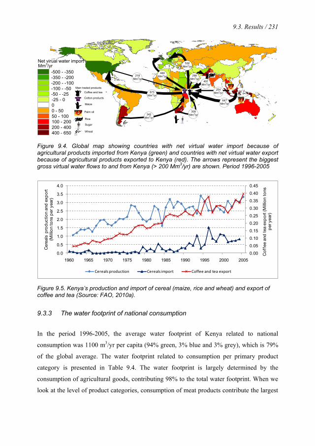
9.3. Results / 231
218 Mm3/yr
342 Mm3/yr
573 Mm3/yr
444 Mm3/yr
532 Mm3/yr
309 Mm3/yr
647 Mm3/yr
254 Mm3/yr
288 Mm3/yr
491 Mm3/yr
-500 - -350-350 - -200-200 - -100-100 - -50-50 - -25-25 - 000 - 5050 - 100100 - 200200 - 400400 - 650
Net virual water importMm3/yr
Coffee and tea
Cotton products
Palm oil
Sugar
Maize
Wheat
Main traded products
Rice
Figure 9.4. Global map showing countries with net virtual water import because of agricultural products imported from Kenya (green) and countries with net virtual water export because of agricultural products exported to Kenya (red). The arrows represent the biggest gross virtual water flows to and from Kenya (> 200 Mm3/yr) are shown. Period 1996-2005
0.00
0.05
0.10
0.15
0.20
0.25
0.30
0.35
0.40
0.45
0.0
0.5
1.0
1.5
2.0
2.5
3.0
3.5
4.0
1960 1965 1970 1975 1980 1985 1990 1995 2000 2005C
offe
e an
d te
a ex
port
(Mill
ion
tons
pe
r yea
r)
Cer
eals
pro
duct
ion
and
expo
rt (M
illio
n to
ns p
er y
ear)
Cereals production Cereals import Coffee and tea export
Figure 9.5. Kenya’s production and import of cereal (maize, rice and wheat) and export of coffee and tea (Source: FAO, 2010a).
9.3.3 The water footprint of national consumption
In the period 1996-2005, the average water footprint of Kenya related to national
consumption was 1100 m3/yr per capita (94% green, 3% blue and 3% grey), which is 79%
of the global average. The water footprint related to consumption per primary product
category is presented in Table 9.4. The water footprint is largely determined by the
consumption of agricultural goods, contributing 98% to the total water footprint. When we
look at the level of product categories, consumption of meat products contribute the largest
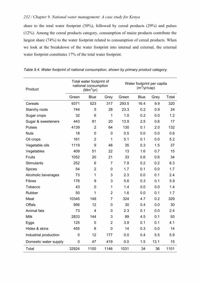
232 / Chapter 9. National water management: A case study for Kenya
share to the total water footprint (30%), followed by cereal products (29%) and pulses
(12%). Among the cereal products category, consumption of maize products contribute the
largest share (74%) to the water footprint related to consumption of cereal products. When
we look at the breakdown of the water footprint into internal and external, the external
water footprint constitutes 17% of the total water footprint.
Table 9.4. Water footprint of national consumption, shown by primary product category.
Product
Total water footprint of national consumption
(Mm3/yr)
Water footprint per capita (m3/yr/cap)
Green Blue Grey Green Blue Grey Total
Cereals 9371 523 317 293.5 16.4 9.9 320 Starchy roots 744 5 28 23.3 0.2 0.9 24 Sugar crops 32 6 1 1.0 0.2 0.0 1.2 Sugar & sweeteners 443 81 20 13.9 2.5 0.6 17 Pulses 4139 2 64 130 0.1 2.0 132 Nuts 18 0 0 0.5 0.0 0.0 0.6 Oil crops 161 2 1 5.1 0.1 0.0 5.2 Vegetable oils 1119 9 48 35 0.3 1.5 37 Vegetables 409 51 22 13 1.6 0.7 15 Fruits 1052 20 21 33 0.6 0.6 34 Stimulants 252 6 7 7.9 0.2 0.2 8.3 Spices 54 2 0 1.7 0.1 0.0 1.7 Alcoholic beverages 73 1 3 2.3 0.0 0.1 2.4 Fibres 178 9 3 5.6 0.3 0.1 5.9 Tobacco 43 0 1 1.4 0.0 0.0 1.4 Rubber 50 1 2 1.6 0.0 0.1 1.7 Meat 10345 149 7 324 4.7 0.2 329 Offals 956 12 0 30 0.4 0.0 30 Animal fats 73 4 0 2.3 0.1 0.0 2.4 Milk 2833 144 3 89 4.5 0.1 93 Eggs 125 5 2 3.9 0.1 0.1 4.1 Hides & skins 455 8 0 14 0.3 0.0 14
Industrial production 0 12 177 0.0 0.4 5.5 5.9
Domestic water supply 0 47 419 0.0 1.5 13.1 15
Total 32924 1100 1146 1031 34 36 1101
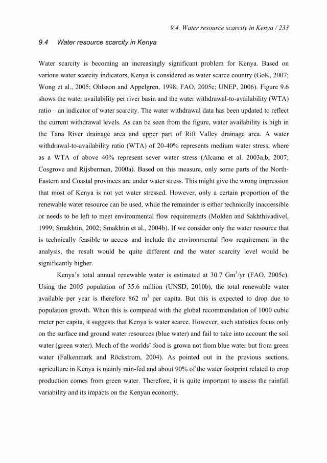
9.4. Water resource scarcity in Kenya / 233
9.4 Water resource scarcity in Kenya
Water scarcity is becoming an increasingly significant problem for Kenya. Based on
various water scarcity indicators, Kenya is considered as water scarce country (GoK, 2007;
Wong et al., 2005; Ohlsson and Appelgren, 1998; FAO, 2005c; UNEP, 2006). Figure 9.6
shows the water availability per river basin and the water withdrawal-to-availability (WTA)
ratio – an indicator of water scarcity. The water withdrawal data has been updated to reflect
the current withdrawal levels. As can be seen from the figure, water availability is high in
the Tana River drainage area and upper part of Rift Valley drainage area. A water
withdrawal-to-availability ratio (WTA) of 20-40% represents medium water stress, where
as a WTA of above 40% represent sever water stress (Alcamo et al. 2003a,b, 2007;
Cosgrove and Rijsberman, 2000a). Based on this measure, only some parts of the North-
Eastern and Coastal provinces are under water stress. This might give the wrong impression
that most of Kenya is not yet water stressed. However, only a certain proportion of the
renewable water resource can be used, while the remainder is either technically inaccessible
or needs to be left to meet environmental flow requirements (Molden and Sakhthivadivel,
1999; Smakhtin, 2002; Smakhtin et al., 2004b). If we consider only the water resource that
is technically feasible to access and include the environmental flow requirement in the
analysis, the result would be quite different and the water scarcity level would be
significantly higher.
Kenya’s total annual renewable water is estimated at 30.7 Gm3/yr (FAO, 2005c).
Using the 2005 population of 35.6 million (UNSD, 2010b), the total renewable water
available per year is therefore 862 m3 per capita. But this is expected to drop due to
population growth. When this is compared with the global recommendation of 1000 cubic
meter per capita, it suggests that Kenya is water scarce. However, such statistics focus only
on the surface and ground water resources (blue water) and fail to take into account the soil
water (green water). Much of the worlds’ food is grown not from blue water but from green
water (Falkenmark and Röckstrom, 2004). As pointed out in the previous sections,
agriculture in Kenya is mainly rain-fed and about 90% of the water footprint related to crop
production comes from green water. Therefore, it is quite important to assess the rainfall
variability and its impacts on the Kenyan economy.
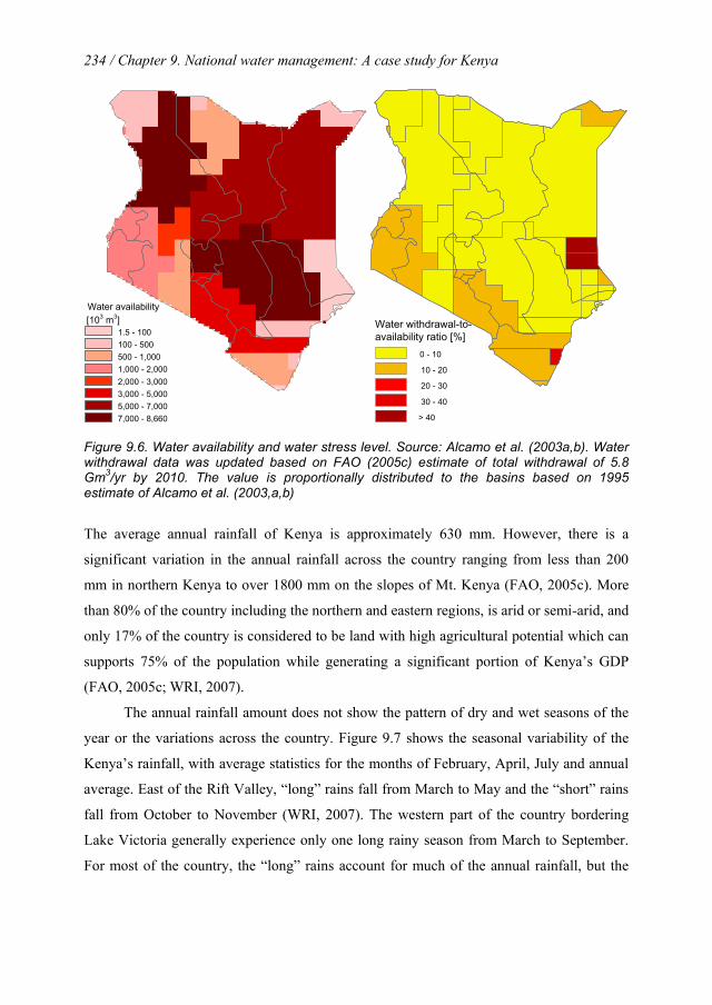
234 / Chapter 9. National water management: A case study for Kenya
Water withdrawal-to-availability ratio [%]
0 - 10
10 - 20
20 - 30
30 - 40
> 40
Water availability[103 m3]
1.5 - 100100 - 500500 - 1,0001,000 - 2,0002,000 - 3,0003,000 - 5,0005,000 - 7,0007,000 - 8,660
Figure 9.6. Water availability and water stress level. Source: Alcamo et al. (2003a,b). Water withdrawal data was updated based on FAO (2005c) estimate of total withdrawal of 5.8 Gm3/yr by 2010. The value is proportionally distributed to the basins based on 1995 estimate of Alcamo et al. (2003,a,b)
The average annual rainfall of Kenya is approximately 630 mm. However, there is a
significant variation in the annual rainfall across the country ranging from less than 200
mm in northern Kenya to over 1800 mm on the slopes of Mt. Kenya (FAO, 2005c). More
than 80% of the country including the northern and eastern regions, is arid or semi-arid, and
only 17% of the country is considered to be land with high agricultural potential which can
supports 75% of the population while generating a significant portion of Kenya’s GDP
(FAO, 2005c; WRI, 2007).
The annual rainfall amount does not show the pattern of dry and wet seasons of the
year or the variations across the country. Figure 9.7 shows the seasonal variability of the
Kenya’s rainfall, with average statistics for the months of February, April, July and annual
average. East of the Rift Valley, “long” rains fall from March to May and the “short” rains
fall from October to November (WRI, 2007). The western part of the country bordering
Lake Victoria generally experience only one long rainy season from March to September.
For most of the country, the “long” rains account for much of the annual rainfall, but the
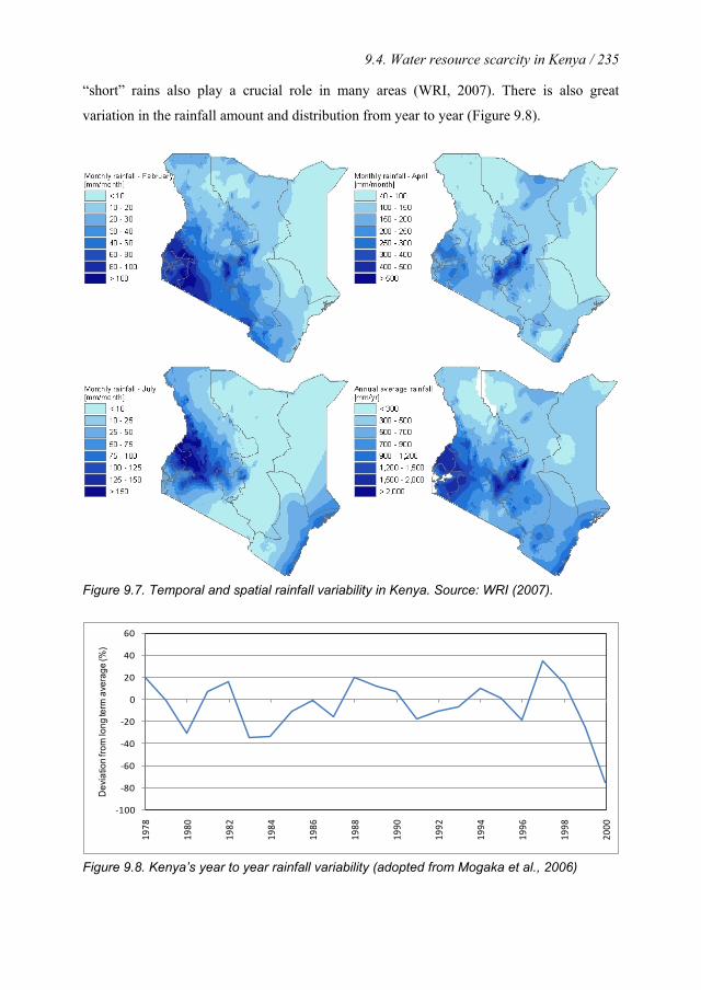
9.4. Water resource scarcity in Kenya / 235
“short” rains also play a crucial role in many areas (WRI, 2007). There is also great
variation in the rainfall amount and distribution from year to year (Figure 9.8).
Figure 9.7. Temporal and spatial rainfall variability in Kenya. Source: WRI (2007).
-100
-80
-60
-40
-20
0
20
40
60
1978
1980
1982
1984
1986
1988
1990
1992
1994
1996
1998
2000
Dev
iatio
n fro
m lo
ng te
rm a
vera
ge (%
)
Figure 9.8. Kenya’s year to year rainfall variability (adopted from Mogaka et al., 2006)
236 / Chapter 9. National water management: A case study for Kenya
Such temporal and spatial variability of rainfall - which most parts of Kenya experience-
combined with high levels of crop water requirement typical in the semi-arid and arid part
of the country precludes much of the country from being suited to the growth of rain-fed
crops. Thus, policy makers should take effective policy measures to manage the water
resource properly in order to avoid future problems with the country’s food production and
economic development.
9.5 Water management in Kenya - the role of virtual water
Managing water scarcity entails either supply-side or demand-side management or a
combination of the two. Since the available water supply is limited in many areas and the
cost of increasing the water supply is usually high, there is a growing emphasis on
increasing water use efficiency (Falkenmark, et al. 2007; Gleick, 1998; Postel, 2000;
Wallace and Gregory, 2002). According to Hoekstra and Hung (2005), there are three
levels at which water use efficiency can be increased. At a local level, namely that of the
water user, water use efficiency can be increased by charging prices based on full marginal
cost, stimulating water-saving technologies, and creating awareness among the water users
on the detrimental impacts of excessive water abstraction. At the river basin level, water
use efficiency can be improved by re-allocating water to those purposes with the highest
marginal benefits. At this level, we speak of ‘water allocation efficiency’. Finally, at the
global level, water use efficiency can be increased if nations use their relative water
abundance or scarcity to either encourage or discourage the use of domestic water resources
for producing export commodities.
As in most countries, Kenya’s irrigation system suffers from poor irrigation
efficiency. About 60% of the irrigated land is irrigated by sprinklers and about 38% by
surface irrigation (FAO, 2005c). Although the potential for water saving through increased
efficiency is high, it is not as large as might be thought (Seckler et al., 2003). This is
because the classical definition of irrigation efficiency ignores the value of return flows i.e.,
irrigation water runoff and seepage that re-enters the water supply system (Keller and
Keller 1995; Seckler et al. 2003). When the return flow is reused, the overall efficiency
increases. Thus, while individual systems could have low levels of efficiency, the basin-
wide efficiencies can be much higher. Therefore, taking steps to increase water use

9.5. Water management in Kenya / 237
efficiency at the local level based on the classical efficiency calculations often will not
result in genuine water savings. The real water savings come not through increasing local
level water use efficiency rather from being as productive as possible with each drop of
water that is consumed. Growing more crops with less water would alleviate water scarcity.
One possible way of increasing water productivity is to raise crop yields at field level.
Figure 9.9 shows that the maize yield in Kenya has shown no improvement over the
years. Although Kenya’s maize yield is slightly above African countries’ average, it is
much below the yield obtained in Egypt, the world average and that of South Africa. This
low yield level is an indication that there is still much room for improvement in Kenya’s
agriculture productivity.
0
1
2
3
4
5
6
7
8
9
1980 1985 1990 1995 2000 2005 2010
Mai
ze y
ield
(ton
/ha)
Kenya World + Africa + South Africa Egypt
Figure 9.9. Kenya's maize yield compared to maize yields in Egypt, South Africa, the continent of Africa and the world. Source: FAO (2010a)
It is evident from Figure 9.10 that the water footprint per tonne of crop in Kenya increases
going from the Western provinces to Eastern and North-Eastern provinces. As pointed out
in other sections, the climate in the North-Eastern, Eastern and Coastal provinces is
characterized as semi-arid or arid. As such, the crop water requirements in these provinces
are quite high compared to the other provinces. The high crop water requirement - coupled
with low water availability - has clearly influenced the crop yields in these areas, which is
well below the other provinces. It is clear from Figure 9.10 that the Western province in
particular has the lowest water footprint per tonne of crop. If crops were to be grown more
238 / Chapter 9. National water management: A case study for Kenya
in the Central, Nairobi Area, Nyanza and Western provinces where the water footprint is
lower, the water saving from such approach would be quite high. However, the decision
about what and where to grow is complex and goes beyond simple water footprint
accountings. If we decide to produce most of the crop in areas of low water footprint,
provided there is enough land and other means of production beside water, how would the
farmers in the marginal areas survive? What alternative means of living would they have?
Such important issues need to be addressed before any measure is taken. Farmers in
particular low income farmers give priority to producing their own food needs rather than
relying on market. Therefore, it is quite important to increase food security, off-farm
income and alternative employment options. Beside this, it might be necessary to assist
farmers to raise their productivity through providing high yielding and drought resistant
crops and improving agricultural techniques so as to obtain more value per unit of water.
Although measures to improve productive efficiency of water as indicated above are
important, the effective way of increasing water productivity is through ‘allocative
efficiency’ (Allan, 1999; Dinar, 1998). The ‘inter-sectoral allocative efficiency’ and the
‘intra-sectoral allocative efficiency’ are two distinct types of a ‘water allocation efficiency’
strategy. The intra-sectoral water allocation efficiency is achieved by allocating water
within the same economic sector from product with low economic return per unit of water
to another product which has a higher economic return per unit of water. This strategy is
more relevant in the agricultural sector in which the range of economic returns gained from
one crop compared with another can be much higher. Figure 9.11 shows productivity
differences among selected crops in Kenya. Cut flowers have a much higher productivity
per unit of water; as much as 250 times more productive than pulses or above 120 times
more productive than maize. Vegetables also have a high water productivity which is very
close to that of cut flower. Spices, fruits and tea also produce more value per unit of water
as compared to the least productive crops. This analysis is consistent with results obtained
by other researchers. Owuor (1998), for example, showed that horticultural crops are more
productive compared to cereal crops such as maize. It is important to stress that the water
productivity is calculated based on the assumption that water is the only scarce resource
and holding other resources such as land, labour and agricultural inputs constant. Besides,
all components of the water footprint (green, blue and grey water) are given equal weight.
If we focus on the blue water footprint only, the figures will completely changes, i.e., the

9.5. Water management in Kenya / 239
non-irrigated crops such as wheat, pulses and tea would have a much higher blue water
productivity compared to cut flower or vegetables. Provided other factors such as
employment opportunities, social equity are addressed, it is beneficial to produce more of
the highly productive crops and earn enough money to import the other least productive
cereal crops. In other words, there should be a policy shift from food self-sufficiency to
food-security. Such decision might involve some form of social stress but not as much as
the inter-sectoral allocative efficiency. The economic befits from intra-sectoral water
allocation is also not as much as the return per unit of water that would be obtained by
inter-sectoral water allocation efficiency.
On the other hand the inter-sectoral water allocation efficiency is achieved through
allocating water from an economic sector with a low return per unit of water, usually
agriculture, to another economic sector which has a higher return per unit of water, usually
industry. Water that is diverted away from agricultural use into industrial and service
sectors can produce as much as 1000 times the economic return per unit of water (Allan,
1999). Allocation efficiency - in particular the inter-sectoral allocative efficiency - is a
highly politically sensitive strategy (Allan, 1999). In a country such as Kenya where about
74% of the population (FAO, 2005c) rely on agriculture as their main source of livelihood,
allocating water away from agriculture to more the productive industry and service sectors
represents a highly socially and politically stressful option (Allan, 1999; Turton and
Ohlsson, 1999). Ohlsson (2000) argues that the conflict which might arise because of re-
allocating water away from agriculture to cities and industries would not be over
competition for the amount of water that is diverted, because small portion of the water
used in agriculture would be enough to satisfy the water requirement of cities and
industries. The possible conflict would rather be about livelihoods of a large population
which might have to be displaced from the agriculture sector. Constraints on industrial and
service sectors capacity to absorb large labour force which are displaced from the
agriculture sector would become highly relevant. The challenge is complex since it would
involve creating new jobs in cities and industries to absorb not only the labour force
displaced from agriculture but also a rapidly growing population.
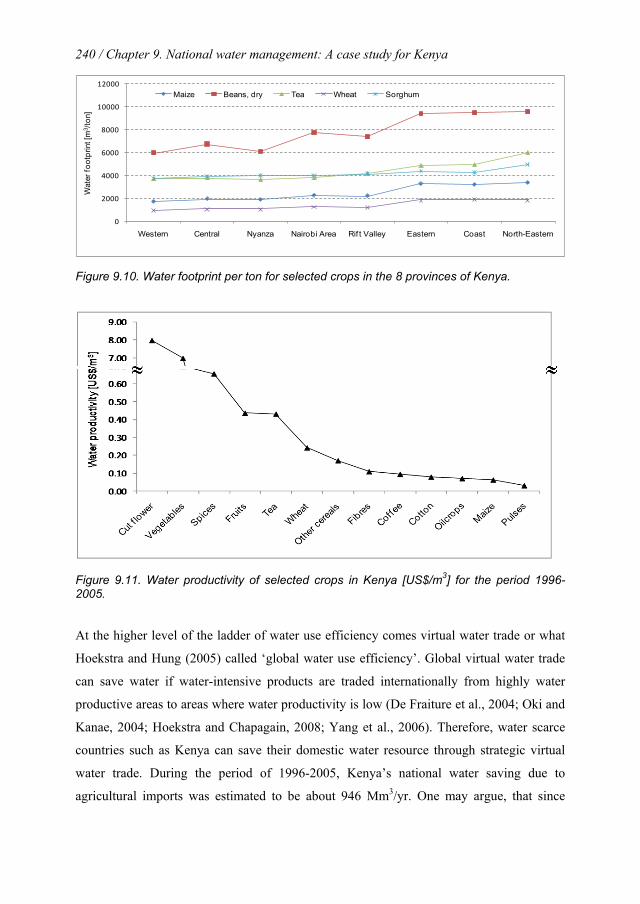
240 / Chapter 9. National water management: A case study for Kenya
0
2000
4000
6000
8000
10000
12000
Western Central Nyanza Nairobi Area Rif t Valley Eastern Coast North-Eastern
Wat
er fo
otpr
int [
m3 /t
on]
Maize Beans, dry Tea Wheat Sorghum
Figure 9.10. Water footprint per ton for selected crops in the 8 provinces of Kenya.
Figure 9.11. Water productivity of selected crops in Kenya [US$/m3] for the period 1996-2005.
At the higher level of the ladder of water use efficiency comes virtual water trade or what
Hoekstra and Hung (2005) called ‘global water use efficiency’. Global virtual water trade
can save water if water-intensive products are traded internationally from highly water
productive areas to areas where water productivity is low (De Fraiture et al., 2004; Oki and
Kanae, 2004; Hoekstra and Chapagain, 2008; Yang et al., 2006). Therefore, water scarce
countries such as Kenya can save their domestic water resource through strategic virtual
water trade. During the period of 1996-2005, Kenya’s national water saving due to
agricultural imports was estimated to be about 946 Mm3/yr. One may argue, that since
9.5. Water management in Kenya / 241
Kenya is basically dependent on rainwater (green water) and the opportunity cost of green
water is minimal, the water saving that would be gained through virtual water import is
minimal. However, as shown in Section 3.2, Kenya’s virtual water export is based mainly
on high-value crops such as coffee, tea and horticultural crops which generate higher return
per unit of water consumed relative to cereal crops such as maize. Its imports, on the other
hand, are mainly low water productivity cereal products. Therefore, cultivating high value
crops with green water as compared to cultivating cereals would generate higher benefit to
Kenya.
Nyoro et al. (2001) showed that Kenya is less competitive compared to its
neighbours, Uganda and Tanzania, in producing the major cereals crops, in particular
maize. The local production cost of maize, sugar (and in some cases wheat) is much higher
than the import parity price. According to Nyoro et al. (2001), the production cost of coffee
is among the highest in the world. Under such conditions, a rational economic decision
might be that Kenya should produce and export crops in which it has comparative
economic advantage and import crops where its comparative advantage is minimal or
negative. However, such policy decisions are never straightforward. It requires a policy
shift from national food self-sufficiency to food security. Such a policy pre-supposes a
strong and diversified economy which provides enough income to pay for the virtual water
import in a sustainable manner. Unless there is enough foreign currency earning from the
export of high productive crops, from the industry and the service sectors, virtual water
import may result in the depletion of the country’s foreign currency reserve. In addition the
local agricultural sector needs to be in a position to be more competitive, otherwise it will
be damaged due to the agricultural goods import. The other important factor which must be
addressed is the creation of employment for the unemployed rural population. In a country
such as Kenya where the great majority of the population rely on the agriculture sector for
their livelihood, a policy shift in the direction of virtual water import may create high social
stress (Allan, 1999; Turton and Ohlsson, 1999). Thus, a careful analysis of all available
options for water management must be made before embracing virtual water trade as a
strategy.

242 / Chapter 9. National water management: A case study for Kenya
9.6 Conclusion
Kenya is not water self-sufficient with respect to its water needs for its own food supply. In
the period 1996-2005, cereal imports contributed 25% of the total supply of the main cereal
products (maize, wheat and rice). On the other hand, a significant part (23%) of the
freshwater consumption and pollution in Kenya is for producing export products.
Through imports of water-intensive goods, Kenya saves 4 Gm3/yr of its scarce water
resources. However, such water saving, should be seen in the context of the risk of losing
food self-sufficiency. It should also be seen in the context of the need to generate foreign
exchange for the import of food and the risk of facing rising and fluctuating world food
prices. Besides, the water saved may not be allocated to other beneficial uses (De Fraiture
et al. 2004).
Over 42% of Kenya’s foreign exchange earnings come from the export of coffee, tea
and horticultural products. These products also contributed about 60% toward the total
virtual water export. The increase in the use of scarce water resource for export products
may, in the long run, conflict with water use for food self-sufficiency.
The production and export of cash crops from developing countries positively
impacts on the socio-economic development of the exporting countries. The water use for
coffee and tea production in Kenya’s Rift Valley is mainly positive: the impacts on the
water system are limited because water use mostly involves the use of rainwater, while the
export revenues amount to US$ 581 million per year, which is 29% of Kenya’s export
value. However, the water use for flower production near Lake Naivasha contributes to
water scarcity (declining lake level) and pollution problems, but the cut flower export
sector is a vital one, contributing US$ 141 million per year in foreign currency, which is
7% of Kenya’s export value. Therefore, it is necessary to design policies that optimize the
trade-offs between the gains from the use of freshwater resources and the high
environmental cost.
In order to address its water scarcity problem, Kenya must implement effective policy
measures at different spatial levels. Such policy measures include: the improvement of
water use efficiency at the user level by charging prices based on full marginal cost,
stimulating water-saving technologies, and creating awareness among the water users on
the detrimental impacts of excessive water abstraction. Charging prices on full marginal
9.6. Conclusion / 243
cost, besides its positive effect on raising water use efficiency, will force farmers to use
water more efficiently and reallocate the limited water to crops which can generate high
economic return per unit of water. Besides, improving water productivity to increase the
benefit per unit of water has large potential in addressing Kenya’s water problem. As
shown in the previous sections, Kenya’s crop yield level is among the lowest in the world.
Raising yields through growing selected seeds and utilization of the available soil moisture
through integrated soil and water management could be quite beneficial. At the river basin
level, water use efficiency can be improved by re-allocating (both intra- and inter-sectoral)
water to those purposes with the highest marginal benefits. Finally, Kenya can use virtual
water import and export as a strategy to address its water problem by discouraging the use
of domestic water resources for producing export commodities which are highly water
intensive and have low economic return per unit of water. Production of crops with high
economic return per unit of water and which are less water intensive and produced from
rain water can be encouraged. A policy mix of measures could be the best alternative to
address Kenya’s water scarcity problem.

10. Mitigating the water footprint of export cut flowers from the lake Naivasha basin, Kenya12
Abstract
Kenya’s cut-flower industry has been praised as an economic success as it contributed an
annual average of US$ 141 million foreign exchange (7% of Kenyan export value) over the
period 1996-2005 and about US$ 352 million in 2005 alone. The industry also provides
employment, income and infrastructure such as schools and hospitals for a large population
around Lake Naivasha. On the other hand, the commercial farms have been blamed for
causing a drop in the lake level and for possibly affecting the lake’s biodiversity. The
objective of this study is to quantify the water footprint within the Lake Naivasha Basin
related to cut flowers and assess the potential for mitigating this footprint by involving cut-
flower traders, retailers and consumers overseas.
The water footprint of one rose flower is estimated to be 7-13 litres. The total virtual
water export related to export of cut flowers from the Lake Naivasha Basin was 16 Mm3/yr
during the period 1996-2005 (22% green water; 45% blue water; 33% grey water). Our
findings show that, although the commercial farms around the lake have contributed to the
decline in the lake level through water abstractions, both the commercial farms and the
smallholder farms in the upper catchment are responsible for the lake pollution due to
nutrient load. The observed decline in the lake level and deterioration of the lake’s
biodiversity calls for sustainable management of the basin through pricing water at its full
cost and other regulatory measures.
Despite broad international agreement on the need for full-cost water pricing,
unilateral efforts to implement it in the agricultural sector are politically difficult, because
farmers have difficulty to accept and local competitiveness may be put at risk. More in
particular, the conditions in Kenya are unlikely to result in serious steps to full-cost pricing,
since many farmers resist even modest water price increases and government is lacking
means of enforcement. In addition, little can be expected from international agreements.
The implementation of an international protocol on water pricing requires global agreement
12 Based on Mekonnen and Hoekstra (2010c).
246 / Chapter 10. Mitigating the water footprint of export cut flowers
among the major players on the global market, which makes it unlikely that such a protocol
will be implemented in the near future. As an alternative to an international water-pricing
protocol we propose an alternative in this study that can be implemented with a focus on
sustainable water use in flower farming around Lake Naivasha alone. The proposal
involves a water-sustainability agreement between major agents along the cut-flower
supply chain and includes a premium to the final product at the retailer end of the supply
chain. Such a ‘water sustainability premium’ will raise awareness among flower consumers
and – when channelled back to the farmers – facilitate the flower farms to install the
necessary equipment and implement the right measures to use water in a sustainable
manner. The collected premiums will generate a fund that can be used for financing
measures to reduce the water footprint and to improve watershed management. The
sustainability premium also reduces the risk of the flower farms losing their
competitiveness and avoids business migration from Kenya to other countries with less
stringent water pricing and environmental regulations.
10.1 Introduction
Lake Naivasha is situated 80 km northwest of Nairobi in the Rift Valley of Kenya (00 45’S,
360 20’E). It is Kenya’s second largest freshwater lake without surface outlet and the
natural fluctuation in water levels over the last 100 years has been in excess of 12 meters
(Mavuti and Harper, 2005). The lake remains fresh due to a significant outflow of
groundwater. The lake has international value as a Ramsar wetland. In the last three
decades, the area around Lake Naivasha has grown to become the main site of Kenya’s
horticultural industry (mainly cut flower), which is the third most important foreign
exchange earner after tea and tourism. Since the late 1990s, the flower farms started to
expand at a faster rate (Becht et al., 2005). The total irrigated commercial farm area around
Lake Naivasha is about 4450 ha. Cut flowers account for about 43% of the irrigated area,
followed by vegetables with 41% and fodder with 15% (Musota, 2008).
The major flower varieties grown and exported from Kenya are roses, carnation,
alstroemeria, lisianthus, statice and cut foliage. Rose flower dominates the export market,
accounting for over 70% of the export volume (HCDA, 2007). The main flower growing
10.1. Introduction / 247
regions are Lake Naivasha, Thika and Kiambu/Limuru (EPZA, 2005b), with Lake Naivasha
accounting for about 95% of the cultivated area.
The lake has attracted attention and concerns from both national and international
organisations. The main stakeholders have shown concern about the health of the lake,
mainly related to the decline of the lake level, deterioration of the water quality and
reduction of biodiversity. Some of the main stakeholders active around the lake are the
Lake Naivasha Riparian Association (LNRA), the Lake Naivasha Growers Group (LNGG)
and Kenya Wildlife Services (KWS). The concerns have led to the development of a
Management Plan in 1996 by the main stakeholders (Becht et. al., 2005). Around that time,
the Lake Naivasha Management Implementation Committee (LNMIC) was formed to
execute the management plan. The plan was officially approved by the Government of
Kenya in 1997.
There have been many studies regarding the lake water balance and the aquatic
ecology of the lake. Most notably, the International Institute of Geo-Information Science
and Earth Observation (ITC), based in the Netherlands, has carried out a number of studies
regarding the lake water balance and nutrient load to the lake and is active in developing a
geo-information system on the land use around the lake. Leicester University and
Earthwatch studied the aquatic ecology of the lake since 1985. Many Kenyan scientists, the
Kenya Marine and Fisheries Research Institute (KEMFRI), Kenya Wildlife Services
(KWS) and Kenya Agricultural Research Institute (KARI) are also doing research on the
lake (Becht et. al., 2005).
The objective of the present study is to quantify the water footprint within the Lake
Naivasha Basin related to horticulture, in particular the flower farms, and assess the
potential for mitigating this footprint by involving cut-flower traders, retailers and
consumers overseas. In addition, we will explore the idea of a voluntary sustainable-flower
agreement between major agents along the flower supply-chain that involves a water-
sustainability premium to be paid by the consumers in the countries importing flowers from
Kenya.
248 / Chapter 10. Mitigating the water footprint of export cut flowers
10.2 Method
The green, blue and grey components of the water footprint of products were calculated
following the method of Hoekstra et al. (2009). The green water footprint refers to the
volume of rainwater consumed; the blue water footprint refers to the volume of surface and
groundwater consumed; the grey water footprint is the volume of freshwater that is required
to assimilate the load of pollutants based on the existing water quality standards. The water
footprint of a crop (m3/ton) is calculated as the ratio of the volume of water (m3/ha)
consumed or polluted during the entire period of crop growth to the corresponding crop
yield (ton/ha). Water consumption has two components: green and blue water consumption.
The grey component of the water footprint of crops (m3/ton) is calculated by dividing the
amount of nitrogen that leaches to the water system (kg/ha) by the maximum acceptable
concentration of nitrogen (kg/m3) and the crop yield (ton/ha).
The crop water requirements, effective rainfall and irrigation requirement for the
different vegetables and cut flower grown around Lake Naivasha were estimated using
CROPWAT (FAO, 2010f). The calculation was done using climatic data obtained from
CLIMWAT (FAO, 2010g) for Naivasha climate station (0.43 0S and 36.26 0E). The cut
flowers are perennial crops and vegetables are grown all over the year with multi-cropping.
Therefore, the blue water footprint for vegetables such as cabbages, onions and tomato was
calculated by running CROPWAT for each planting cycle.
For the other 22 crops grown in the upper catchment of the Lake Naivasha Basin, a
crop water use model (Mekonnen and Hoekstra, 2010a) was used to carry out a daily soil
water balance and calculate the green, blue and grey water footprint at grid level. The
model was run for the whole of Kenya and later the Lake Naivasha Basin area raster was
used to extract data applicable only for the basin.
Virtual water exports (m3/yr) related to exports of cut flowers and vegetables were
calculated by multiplying the trade volumes (tons/yr) by their respective water footprint in
Kenya (m3/ton).
10.3. Data / 249
10.3 Data
The Lake Naivasha Basin is schematised here into two parts: the upper catchment with
smallholder farms and the area around Lake Naivasha with big farms producing for export.
Grid data on type and size of farms around Lake Naivasha was obtained from the ITC
Naivasha database (Becht, 2007). For crops grown in the upper catchment, the crop
growing areas with 5 arc minute grid cell resolution (which is equivalent to 9.3×9.3 km2
around Naivasha) were obtained from Monfreda et al. (2008). The grid crop area data was
aggregated to a national level and compared with and scaled to fit national average crop
harvest area for the period 1996-2005 obtained from FAOSTAT (FAO, 2010a).
The cut-flower production for the period 1996-2005 around Lake Naivasha was
calculated from the export data assuming that 95% of the cut-flower production is exported.
The crop parameters (crop coefficients and start and length of cropping seasons) for
the different vegetables were taken from Chapagain and Hoekstra (2004). For cut flowers,
the crop parameters were adopted from Orr and Chapagain (2006). The evapotranspiration
in greenhouse conditions is assumed to be 65% of the outdoor condition as suggested by
various authors (Mpusia, 2006; Baille et al., 1994; Orgaz et al., 2005). The average water
footprint of cut flowers was estimated based on the weighted average of indoor and outdoor
farm areas. About 62% of the cut flowers around Lake Naivasha are grown in greenhouses
(Musota, 2008). Table 10.1 gives the irrigated area and fertilizer application rate for
irrigated crops around Lake Naivasha. A leaching-runoff fraction of 10% was assumed,
following Hoekstra and Chapagain (2008).
Grid-based soil moisture data of total available water capacity (TAWC) at 5 arc
minute resolution was taken from ISRIC-WISE (Batjes, 2006). An average value of TAWC
of the five soil layers was used in the model. The main data source for nitrogen fertilizer
application rate per crop for the upper catchment was FAO (2010c).
Data on irrigated area per crop was obtained mainly from the AQUASTAT country
profile database (FAO, 2005c) and Portmann et al. (2008). For rice, data on irrigated area
was obtained from EPZA (2005a). The country level irrigated area data is distributed to
grid cells according to area equipped for irrigation (AEI). The Global Map of Irrigation
Areas version 4.0.1 (Siebert et al., 2007) with spatial resolution of 5 arc minute was used to
define the area equipped for irrigation for each grid cell. The distribution was done

250 / Chapter 10. Mitigating the water footprint of export cut flowers
proportional to the harvested area of each cropped grid cell. For cases where there is no
AEI data or the AEI does not match with the irrigated area data, the irrigation area data is
distributed proportional to the harvest area of each cropped grid cell.
Table 10.1. Irrigated crops around Lake Naivasha. Year 2006.
Crop Irrigated area* Fertilizer application rate (kg/ha)**
Area (ha) % N P2O5 K2O
Total flowers 1911 42.8 325 145 303
Roses 1028 23.0 325 145 303
Roses & carnations 730 16.3 325 145 303
Roses, hypercium 21 0.5 325 145 303
Other flowers 132 3.0 325 145 303
Total vegetables 1824 40.8 185 179 55
Babycorn 205 4.6 41 113 0
Babycorn & beans 143 3.2 252 141 81
Babycorn, beans & cabbage 169 3.8 235 141 81
Babycorn, beans & onions 906 20.3 244 244 81
Beans/tomatoes 21 0.5 235 141 81
Cabbage 374 8.4 68 94 0
Cabbage & beans 6 0.1 235 141 81
Total fodder 665 14.9 68 94 0
Grass 286 6.4 68 94 0
Grass & lucerne 40 0.9 68 94 0
Lucerne 163 3.7 68 94 0
Lucerne, babycorn, beans 176 3.9 68 94 0
Macadamia 50 1.1 68 94 0
Eucalyptus 17 0.4
Total 4467 100.0 * Musota (2008), ITC Naivasha database (Becht, 2007). ** Tiruneh (2004), Xu (1999), Ariga et al. (2006).
Average monthly reference evapotranspiration data at 10 arc minute resolution were
obtained from FAO (2010d). The 10 minute data was converted to 5 arc minute resolution
10.4. Water use within the Lake Naivasha Basin / 251
by assigning the 10 minute data to each of the four 5 minute grid cells. Following the
CROPWAT approach, the monthly average data was converted to daily values by curve
fitting to the monthly average through polynomial interpolation.
Monthly values for precipitation, wet days, minimum and maximum temperature
with a spatial resolution of 30 arc minute were obtained from CRU through CGIAR-CSI
GeoPortal (Mitchell and Jones, 2005). The 30 arc minute data were assigned to each of the
thirty-six 5 arc minute grid cells contained in the 30 arc minute grid cell. Daily precipitation
values were generated from these monthly average values using the CRU-dGen daily
weather generator model (Schuol and Abbaspour, 2007).
Data on trade in cut flowers and vegetable products in the period 1996-2005 have
been taken from the SITA (Statistics for International Trade Analysis) database available
from the International Trade Centre (ITC, 2007).
10.4 Water use within the Lake Naivasha Basin related to cut-flower production
10.4.1 The water footprint within the Lake Naivasha Basin related to crop
production
The water footprint related to crop production in the Lake Naivasha Basin is presented in
Table 10.2. Two groups of crops are shown: fully irrigated crops grown by commercial
farms mainly for export and concentrated around Lake Naivasha, and other crops which are
cultivated by small farmers in the upper catchment. The total water footprint related to crop
production sums up to 102 Mm3/yr. About 68.7% of the water footprint is related to green
water, 18.5% blue water and 12.8% grey water. The commercial crops contribute 41% to
the total water footprint related to crop production. About 98% (18.4 Mm3/yr) of the blue
water footprint and about 61% of the grey water footprint in the catchment area can be
attributed to the commercial farms around the lake.
In addition to the irrigated farms which are found around Lake Naivasha, the basin is
used mainly for cattle and game rangeland. Smallholder farmers growing mainly maize,
vegetables and other crops occupy areas which receive high rainfall. There are about
18,000 ha of farm land in the upper catchment of which only 2% is irrigated. The average
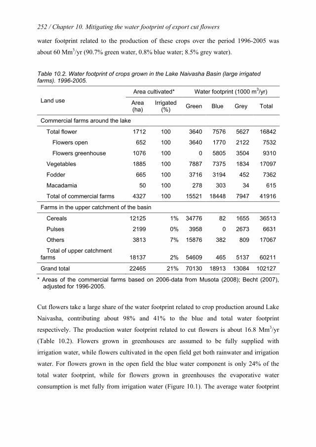
252 / Chapter 10. Mitigating the water footprint of export cut flowers
water footprint related to the production of these crops over the period 1996-2005 was
about 60 Mm3/yr (90.7% green water, 0.8% blue water; 8.5% grey water).
Table 10.2. Water footprint of crops grown in the Lake Naivasha Basin (large irrigated farms). 1996-2005.
Land use Area cultivated* Water footprint (1000 m3/yr)
Area (ha)
Irrigated (%) Green Blue Grey Total
Commercial farms around the lake
Total flower 1712 100 3640 7576 5627 16842
Flowers open 652 100 3640 1770 2122 7532
Flowers greenhouse 1076 100 0 5805 3504 9310
Vegetables 1885 100 7887 7375 1834 17097
Fodder 665 100 3716 3194 452 7362
Macadamia 50 100 278 303 34 615
Total of commercial farms 4327 100 15521 18448 7947 41916
Farms in the upper catchment of the basin
Cereals 12125 1% 34776 82 1655 36513
Pulses 2199 0% 3958 0 2673 6631
Others 3813 7% 15876 382 809 17067
Total of upper catchment farms 18137 2% 54609 465 5137 60211
Grand total 22465 21% 70130 18913 13084 102127
* Areas of the commercial farms based on 2006-data from Musota (2008); Becht (2007), adjusted for 1996-2005.
Cut flowers take a large share of the water footprint related to crop production around Lake
Naivasha, contributing about 98% and 41% to the blue and total water footprint
respectively. The production water footprint related to cut flowers is about 16.8 Mm3/yr
(Table 10.2). Flowers grown in greenhouses are assumed to be fully supplied with
irrigation water, while flowers cultivated in the open field get both rainwater and irrigation
water. For flowers grown in the open field the blue water component is only 24% of the
total water footprint, while for flowers grown in greenhouses the evaporative water
consumption is met fully from irrigation water (Figure 10.1). The average water footprint

10.4. Water use within the Lake Naivasha Basin / 253
of cut flowers grown around Lake Naivasha is 367 m3/ton. About 45% (165 m3/ton) of this
water footprint refers to blue water, 22% (79 m3/ton) to green water and 33% (123 m3/ton)
to grey water, the volume of water needed to assimilate the nitrogen fertilisers that enter the
water systems due to leaching or runoff.
The six big farms – Logonot Horticulture, Delamere, Oserian, Gordon-Miller,
Marula Estate and Sher Agencies – account for about 56% of the total operational water
footprint around Lake Naivasha and 60% of the blue water footprint related to crop
production.
10.4.2 The water footprint per cut flower
Depending on the yield and weight of a rose flower stem, the water footprint per stem
varies from 7 to 13 litre/stem (Table 10.3). If we assume an average rose flower stem
weights about 25 gram, its green water footprint would be 2 litre/stem, its blue water
footprint 4 litre/stem and its grey water footprint 3 litre/stem, resulting in a total water
footprint of 9 litre per stem.
Figure 10.1. Water footprint per ton of crop for crops grown around the lake. Period 1996-2005

254 / Chapter 10. Mitigating the water footprint of export cut flowers
Table 10.3. The water footprint of a rose flower. Period 1996-2005.
Weight of rose (gram/stem)
Cut flower production (stem/m2)
Water footprint by type (litre/stem)
Green Blue Grey Total
20 134 1.6 3.3 2.5 7.3
25 107 2.0 4.1 3.1 9.2
35 77 2.8 5.8 4.3 12.8
10.4.3 Virtual water export from the Lake Naivasha Basin
When we assume that about 95% of Kenya’s cut-flowers export comes from the area
around Lake Naivasha, the average virtual water export from the Lake Naivasha Basin
related to export of cut flowers was 16 Mm3/yr in the period 1996-2005 (22% green water,
45% blue water and 33% grey water) (Table 10.4). The European Union is Kenya’s
principal market for cut flowers; with the Netherlands, the UK, and Germany together
taking over 90 percent of the virtual water export due to export of cut flowers. The
Netherlands is the principal market, accounting for 69% of the total export, followed by the
UK with 18% and Germany with 7%. The virtual water export in relation to export of cut
flowers has shown a significant growth, with virtual water export almost doubling from 11
Mm3/yr in 1996 to 21 Mm3/yr in 2005.
In addition to cut flowers, vegetables such as beans, sweet corn, tomato, cabbage and
onions are produced for both export and domestic consumption. About 50% of the
vegetable produced around Lake Naivasha is exported and the remaining is supplied to
local markets, mainly to Nairobi. The virtual water export related to vegetable products was
8.5 Mm3/yr. Most of the virtual water related to vegetable products was exported to the
United Arab Emirates, France and the United Kingdom. Therefore, for the period 1996-
2005, the total virtual water export related to export of cut flowers and vegetable products
was 24.5 Mm3/yr.
The cut-flower industry is an important export sector, which contributed an annual
average of US$ 141 million foreign exchange (7% of Kenyan export value) over the period
1996-2005, and US$ 352 in 2005 alone. Hence, Kenya is generating foreign exchange of
(141/16=) 8.8 US$/m3.
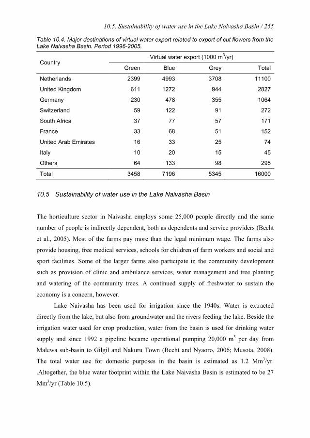
10.5. Sustainability of water use in the Lake Naivasha Basin / 255
Table 10.4. Major destinations of virtual water export related to export of cut flowers from the Lake Naivasha Basin. Period 1996-2005.
Country Virtual water export (1000 m3/yr)
Green Blue Grey Total
Netherlands 2399 4993 3708 11100
United Kingdom 611 1272 944 2827
Germany 230 478 355 1064
Switzerland 59 122 91 272
South Africa 37 77 57 171
France 33 68 51 152
United Arab Emirates 16 33 25 74
Italy 10 20 15 45
Others 64 133 98 295
Total 3458 7196 5345 16000
10.5 Sustainability of water use in the Lake Naivasha Basin
The horticulture sector in Naivasha employs some 25,000 people directly and the same
number of people is indirectly dependent, both as dependents and service providers (Becht
et al., 2005). Most of the farms pay more than the legal minimum wage. The farms also
provide housing, free medical services, schools for children of farm workers and social and
sport facilities. Some of the larger farms also participate in the community development
such as provision of clinic and ambulance services, water management and tree planting
and watering of the community trees. A continued supply of freshwater to sustain the
economy is a concern, however.
Lake Naivasha has been used for irrigation since the 1940s. Water is extracted
directly from the lake, but also from groundwater and the rivers feeding the lake. Beside the
irrigation water used for crop production, water from the basin is used for drinking water
supply and since 1992 a pipeline became operational pumping 20,000 m3 per day from
Malewa sub-basin to Gilgil and Nakuru Town (Becht and Nyaoro, 2006; Musota, 2008).
The total water use for domestic purposes in the basin is estimated as 1.2 Mm3/yr.
.Altogether, the blue water footprint within the Lake Naivasha Basin is estimated to be 27
Mm3/yr (Table 10.5).
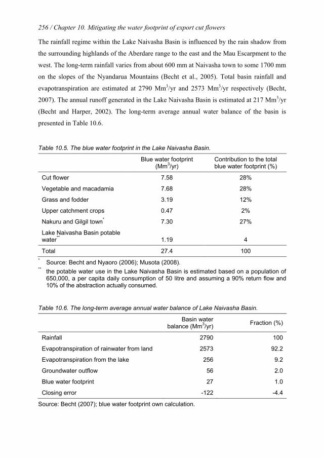
256 / Chapter 10. Mitigating the water footprint of export cut flowers
The rainfall regime within the Lake Naivasha Basin is influenced by the rain shadow from
the surrounding highlands of the Aberdare range to the east and the Mau Escarpment to the
west. The long-term rainfall varies from about 600 mm at Naivasha town to some 1700 mm
on the slopes of the Nyandarua Mountains (Becht et al., 2005). Total basin rainfall and
evapotranspiration are estimated at 2790 Mm3/yr and 2573 Mm3/yr respectively (Becht,
2007). The annual runoff generated in the Lake Naivasha Basin is estimated at 217 Mm3/yr
(Becht and Harper, 2002). The long-term average annual water balance of the basin is
presented in Table 10.6.
Table 10.5. The blue water footprint in the Lake Naivasha Basin.
Blue water footprint (Mm3/yr)
Contribution to the total blue water footprint (%)
Cut flower 7.58 28%
Vegetable and macadamia 7.68 28%
Grass and fodder 3.19 12%
Upper catchment crops 0.47 2%
Nakuru and Gilgil town* 7.30 27%
Lake Naivasha Basin potable water** 1.19 4
Total 27.4 100 * Source: Becht and Nyaoro (2006); Musota (2008). ** the potable water use in the Lake Naivasha Basin is estimated based on a population of
650,000, a per capita daily consumption of 50 litre and assuming a 90% return flow and 10% of the abstraction actually consumed.
Table 10.6. The long-term average annual water balance of Lake Naivasha Basin.
Basin water balance (Mm3/yr) Fraction (%)
Rainfall 2790 100
Evapotranspiration of rainwater from land 2573 92.2
Evapotranspiration from the lake 256 9.2
Groundwater outflow 56 2.0
Blue water footprint 27 1.0
Closing error -122 -4.4
Source: Becht (2007); blue water footprint own calculation.
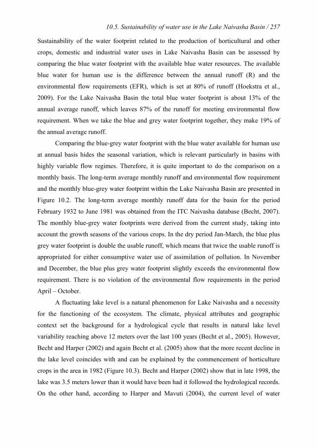
10.5. Sustainability of water use in the Lake Naivasha Basin / 257
Sustainability of the water footprint related to the production of horticultural and other
crops, domestic and industrial water uses in Lake Naivasha Basin can be assessed by
comparing the blue water footprint with the available blue water resources. The available
blue water for human use is the difference between the annual runoff (R) and the
environmental flow requirements (EFR), which is set at 80% of runoff (Hoekstra et al.,
2009). For the Lake Naivasha Basin the total blue water footprint is about 13% of the
annual average runoff, which leaves 87% of the runoff for meeting environmental flow
requirement. When we take the blue and grey water footprint together, they make 19% of
the annual average runoff.
Comparing the blue-grey water footprint with the blue water available for human use
at annual basis hides the seasonal variation, which is relevant particularly in basins with
highly variable flow regimes. Therefore, it is quite important to do the comparison on a
monthly basis. The long-term average monthly runoff and environmental flow requirement
and the monthly blue-grey water footprint within the Lake Naivasha Basin are presented in
Figure 10.2. The long-term average monthly runoff data for the basin for the period
February 1932 to June 1981 was obtained from the ITC Naivasha database (Becht, 2007).
The monthly blue-grey water footprints were derived from the current study, taking into
account the growth seasons of the various crops. In the dry period Jan-March, the blue plus
grey water footprint is double the usable runoff, which means that twice the usable runoff is
appropriated for either consumptive water use of assimilation of pollution. In November
and December, the blue plus grey water footprint slightly exceeds the environmental flow
requirement. There is no violation of the environmental flow requirements in the period
April – October.
A fluctuating lake level is a natural phenomenon for Lake Naivasha and a necessity
for the functioning of the ecosystem. The climate, physical attributes and geographic
context set the background for a hydrological cycle that results in natural lake level
variability reaching above 12 meters over the last 100 years (Becht et al., 2005). However,
Becht and Harper (2002) and again Becht et al. (2005) show that the more recent decline in
the lake level coincides with and can be explained by the commencement of horticulture
crops in the area in 1982 (Figure 10.3). Becht and Harper (2002) show that in late 1998, the
lake was 3.5 meters lower than it would have been had it followed the hydrological records.
On the other hand, according to Harper and Mavuti (2004), the current level of water
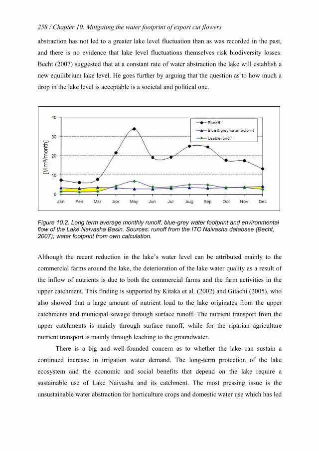
258 / Chapter 10. Mitigating the water footprint of export cut flowers
abstraction has not led to a greater lake level fluctuation than as was recorded in the past,
and there is no evidence that lake level fluctuations themselves risk biodiversity losses.
Becht (2007) suggested that at a constant rate of water abstraction the lake will establish a
new equilibrium lake level. He goes further by arguing that the question as to how much a
drop in the lake level is acceptable is a societal and political one.
Figure 10.2. Long term average monthly runoff, blue-grey water footprint and environmental flow of the Lake Naivasha Basin. Sources: runoff from the ITC Naivasha database (Becht, 2007); water footprint from own calculation.
Although the recent reduction in the lake’s water level can be attributed mainly to the
commercial farms around the lake, the deterioration of the lake water quality as a result of
the inflow of nutrients is due to both the commercial farms and the farm activities in the
upper catchment. This finding is supported by Kitaka et al. (2002) and Gitachi (2005), who
also showed that a large amount of nutrient load to the lake originates from the upper
catchments and municipal sewage through surface runoff. The nutrient transport from the
upper catchments is mainly through surface runoff, while for the riparian agriculture
nutrient transport is mainly through leaching to the groundwater.
There is a big and well-founded concern as to whether the lake can sustain a
continued increase in irrigation water demand. The long-term protection of the lake
ecosystem and the economic and social benefits that depend on the lake require a
sustainable use of Lake Naivasha and its catchment. The most pressing issue is the
unsustainable water abstraction for horticulture crops and domestic water use which has led

10.5. Sustainability of water use in the Lake Naivasha Basin / 259
to a decline in the lake level (Becht and Harper, 2002). There is further the concern about
eutrophication of the lake due to an increase in agricultural nutrients inflow both from the
commercial farms and from the upper catchment. The increase in nutrients is probably the
combined effect of the loss of riparian vegetation, which acts as a buffer to trap sediments,
an increase in the sediment flow from the catchment and an increase in fertilisers leaching
and running off to the water system. The situation got worse by the increase in subsistence
farming even on steep slopes right down to the river edge which destroyed the riparian zone
(Everard and Harper 2002).
Calculated lake level without accounting for
water abstraction
Figure 10.3. Long-term water level change in Lake Naivasha. The calculated lake level represents the case without water abstraction (reproduced from Becht et al, 2005).
Long-term gains from a sustainable and wise use of water require a coordinated action at
the catchment scale. There is a need to define the maximum allowable water abstraction
level at the basin scale. Although equitable allocation of water is required, decisions should
also take into account the difference in economic water productivity among different crops.
Cut flowers generate more economic return than the low-value fodder crops and grasses.
Indoor flowers are more efficient compared to outdoor flowers; therefore greenhouse
cultivation coupled with rainwater harvesting should be encouraged. The use of blue water
for the production of water-intensive products such as beans and low-value products such
as grass and fodder should be discouraged. Wise use of rainwater, in particular in the upper
catchment, for growing fodder and grass needs to be encouraged. Controlling of unlicensed
and illegal water abstraction through legal means and community involvement is quite
essential.
260 / Chapter 10. Mitigating the water footprint of export cut flowers
There is a need to reduce the flow of sediments and agricultural nutrients to the lake both
from the commercial farms around the lake and subsistence farmers in the upper catchment.
The sedimentation problem is aggravated due to the loss of riparian vegetation that could
have acted as a buffer in trapping sediments and increasing infiltration. An urgent and
coordinated action is needed to stop the destruction of vegetation along the river banks and
lake caused by cultivation and overgrazing. Therefore, prohibition of cultivation in the
riparian areas is important.
10.6 Reducing the water footprint in the Lake Naivasha Basin: involving
consumers, retailers and traders along the supply chain
10.6.1 Current water regulations in the Lake Naivasha Basin
Kenya’s water sector reform has gone a long way before the adoption of the Water Act in
2002. The first water sector reform in Kenya was in 1974, when the first National Water
Master Plan was launched (Kisima, 2007). The publication of the ‘Sessional Paper No. 1 of
1999 on National Policy on Water Resources Management and Development’ led to a new
momentum (Owuor and Foeken, 2009). The Water Act 2002 has introduced comprehensive
and, in many instances, radical changes to the legal framework for the management of the
water sector in Kenya (Mumma, 2005). The National Water Resources Management
Strategy document specifies ten ‘specific objectives’. Among these are (Owuor and
Foeken, 2009): (a) manage the water demand in a sustainable way, and (b) water pricing
that recognizes water as an economic good.
Kenyan government considers water as both a social and economic good, to be
available for all Kenyans and at a price reflecting its market value. This principle is
reflected in the different water sector strategies and water resource management rules.
Among the strategies pursued are demand management, the re-allocation of water to where
it has high return and efficient allocation of water through appropriate pricing.
As water is becoming an increasingly scarce resource, full-cost pricing of water is
recognized as an effective tool for its management. The need to have full-cost pricing of
water has received worldwide acknowledgement since the International Conference on
Water and the Environment held in Dublin, 1992. Agenda 21 of the United Nations (UN,
10.6. Reducing the water footprint in the Lake Naivasha Basin / 261
1992) further supported the internalization of environmental costs and the use of economic
instruments for rational use of water resources. The World Water Commission (2000)
stated that ‘the single most immediate and important measure that we can recommend is the
systematic adoption of full-cost pricing for water services’. Hoekstra (2006) and Rogers et
al. (2002) argue that sustainable and efficient use of water requires full-cost pricing of
water use, including all cost components: the operation and maintenance costs, capital
costs, opportunity costs, scarcity rent and externality costs of water use.
However, there are few successful examples of implemented full-cost pricing of
water (Cornish et al. 2004; Rosegrant and Cline, 2002; Dinar and Subramanian, 1998). In
most OECD countries, let alone in developing countries, the implementation of water
pricing policies has been slow and uneven (Molle and Berkoff, 2007; Perry, 2003;
Rosergrant and Cline, 2002). The World Bank (2004) acknowledged the complexity of
water pricing reform (both in theory and practice) for irrigation. It further advocates a
‘pragmatic but principled’ approach that respects principles of efficiency, equity and
sustainability while recognizing that water resources management is intensely political and
that reform requires the articulation of prioritized, sequenced, practical and patient
interventions.
Lack of funding is one of the main challenges in the Lake Naivasha Basin for
implementing community-based basin rehabilitation and lake conservation (Becht et al.
2005). Under such condition, raising enough funds would be an additional objective of
water pricing, besides creation of an incentive for efficient and sustainable use of water.
However, the implementation of full marginal-cost pricing under the existing conditions in
Kenya and around Naivasha is highly unlikely. The flower farms feel that they are already
overtaxed and burdened with a number of remittances and some even have threatened to
relocate to Ethiopia if local authorities force them to pay more tax (Riungu, 2007).
Attracted by a number of incentives including 10 year tax-holidays, better security, duty-
free import of capital goods and low land price, five major flower companies have already
made the switch to Ethiopia with more to follow (ARB, 2007).
According to the 2007 Water Resource Management Rules, domestic water users
have to pay 0.50 Kenyan Shilling per m3 and non-domestic water users have to pay 0.50 to
0.75 Kenyan Shilling per m3. Major water users need a license to abstract water and need to
install water meters. Implementation of the regulation is actually hampered, however, by
262 / Chapter 10. Mitigating the water footprint of export cut flowers
reluctance of many water users to follow the regulation and difficulties government
encounters in enforcing the regulation. The current water pricing policy has several
weaknesses. One is that illegal water abstractions from both ground- and surface water are
very common. In practice it is difficult for the government to check whether farmers,
particularly in the upper catchment, have actually installed water meters as legally required,
due to a lack of cars and fuel for the staff responsible for control. Despite the fact that
farmers have indicated that the newly introduced water tariff is too high, the tariff actually
does by far not cover full economic cost of the water. As a result, the funds generated by
the current water pricing scheme are very small. The level of water price increase that
would be required to have a significant impact on demand would be politically very
difficult to enforce.
Under such conditions, the implementation of full-cost water pricing at the source is
not feasible. A unilateral implementation of a stringent water pricing strategy by a country
could affect the competitiveness of its local companies in the global market (Hoekstra,
2006; Cornish et al. 2004). To address this problem, Hoekstra (2006) have proposed that
national governments negotiate on an international protocol on water pricing. Such scheme
would reduce the disadvantage of unilateral implementation of a full-cost pricing strategy.
However, the implementation of an international protocol on water pricing requires global
agreement among the major players on the global market, which makes it unlikely that such
a protocol will be implemented in the near future. As an alternative to the international
protocol involving national governments we propose an alternative here that can be
implemented with a focus on sustainable water use in flower farming around Lake
Naivasha alone. The proposal involves a water-sustainability agreement between major
agents along the cut-flower supply chain and includes a premium to the final product at the
retailer end of the supply chain.
10.6.2 A sustainable-flower agreement between major agents along the cut-flower
supply-chain
Given the recent emergence of more environmentally conscious consumers, combined with
an increased interest at the side of traders and retailers in providing environmentally
sustainable consumer products, involving consumers and other stakeholders forms an

10.6. Reducing the water footprint in the Lake Naivasha Basin / 263
opportunity to achieve sustainable water use in cut-flower production. Consumers are
becoming more and more concerned with how their consumption behaviour is affecting the
world around them. This is reflected in the growing consumption of fair-trade products and
organic produce. Annual growth rates of 20 percent or more in market volume have been
observed for many years for both organic and fair-trade products (Poisot et al. 2007; Krier,
2005). Several studies show that consumers are willing to pay more for products that are
environmentally and socially responsible (Aizaki and Sato, 2007; Arnot et al. 2006; Didier
and Lucie, 2008; Pelsmacker et al. 2005).
In this section we describe the possible characteristics of a ‘sustainable-flower
agreement’ between major agents along the flower supply-chain focused on sustainable
water use. The agreement should include two key ingredients: a fund-raising mechanism at
the consumer-end of the supply chain, which will raise the funds for making water use in
flower production sustainable, and a labelling or certification scheme, which will provide
the guarantee that the funds are properly spent and that the flower production actually
moves in the direction of sustainable water use.
Funds. The premium collected when selling cut flowers from the Lake Naivasha Basin to
consumers in the Netherlands, the UK etc. should be used to invest in better watershed
management and, most in particular, in reducing the water footprint of the flower farmers.
Clear criteria need to be formulated for how collected funds can or should be spent. The
criteria could be formulated such that also small farmers belong to the beneficiaries of the
funds, because particularly smallholder farmers have generally more difficulty than the
large farmers to comply with environmental standards or raise funds to be able to comply.
There is a need to provide institutional infrastructure through which the funds could
flow back to the basin and be used in environmental protection, watershed management,
support of farmers to improve their water management and community development. Fair-
trade organisations can be instrumental in making sure that funds raised at the consumer
end flow back to the watershed for the support of local programmes for improved
watershed management and support to farmers to reduce their water footprint. Figure 10.4
is a visual representation of the cut-flower supply chain and contrasts the current approach
of local water pricing with the approach of collecting a water-sustainability premium at the
end of the chain.

264 / Chapter 10. Mitigating the water footprint of export cut flowers
The funds that can be raised through adding a water-sustainability premium at the end of
the supply chain (at the consumer end) are much larger than the funds potentially raised
from the current local water-pricing policy (Table 10.7). Currently, the water abstraction
fee in Kenya for commercial farmers is 0.50 Kenyan Shillings per cubic meter of water
abstracted (0.007 €/m3). The total water abstraction by the commercial farms around the
lake is estimated at 40 Mm3/yr and out this the flower farms receive about 50% (Becht,
2007). With a water abstraction fee of 0.007 €/m3, this would raise 0.13 million €/yr. Given
an annual cut-flower export of 1.7 billion stems, they will thus pay, on average, 0.000076 €
per stem of cut flower for abstracting irrigation water. This is a very optimistic estimate,
because as explained before, the conditions are not such that government is actually able to
enforce farmers to pay. On the other hand, if we assume a water sustainability premium of
0.01 € per stem of cut flower at the retailer, to be paid by the consumer, one would raise
16.9 million €/yr (Table 10.7). When we look at the capability of generating funds for
watershed management, we find that a water-sustainability premium raised at the consumer
end of the supply-chain will yield hundred to two hundred times the amount of money
potentially raised through local water pricing.
Flower farms Flower traders Retailers Consumers Water use Catchment
hydrology
Current water pricing policy
Water sustainability premium to final product
Investment in reducing water footprint and improving
Figure 10.4. Schematization of the flower supply-chain. Local water pricing is a mechanism applied at the beginning of the chain; a water-sustainability premium is raised at the end of the chain. Due to the increase of the price per flower along the supply-chain, generating funds is easier at the end of the chain.
Certification/labelling. Collecting a water-sustainability premium at the lower end of the
supply chain needs to go hand in hand with a mechanism for certification of the farmers
that deliver the premium-flowers and a mechanism for labelling the premium-flowers.
Labelling can be interpreted here in physical sense – where indeed a consumer-oriented
10.6. Reducing the water footprint in the Lake Naivasha Basin / 265
label is attached to a flower – but it can also get the shape of ‘attached information’ to
whole batches of flowers. Customers can be encouraged to buy flowers from certified farms
or labelled flowers and pay an agreed premium to contribute to the sustainability of
production and consumption. Certification and labelling would help to segregate
environmentally sustainable products from other products and provide consumers with the
quality assurance. The success depends on a transparent, credible monitoring and
certification systems. Farmers would benefit by having an advantage on the market by
achieving standards of production that are internationally recognized.
Table 10.7. Comparison of revenue collection through the current water-pricing policy and through a water-sustainability premium per cut flower sold to the consumer.
Current water pricing
Water sustainability premium to final product
at retailer
Water abstraction fee (€/m3) 0.007
Total blue water abstraction by flower farms (Mm3/yr) 20
Revenue per stem of flower (€/stem) 0.000076 0.01
Flower export* (tons/yr) 42300
Flower export*,** (stems/yr) 1.69E+09
Estimated revenue (€/yr) 0.13E+06 16.9E+06 * Average for the period: 1996-2005. ** Assumed 25 gram/stem.
The certification of farmers and labelling of products could be carried out by the already
existing institutional setup of Global Good Agricultural Practices (GlobalGAP). The water-
sustainability standards can possibly be integrated into the existing standards of
GlobalGAP. GAP is already applied in many developed and developing countries including
Kenya. Farmers who have complied with the GlobalGAP have benefited in the form of
increased access to market, increased productivity and reduced cost of production through
careful application of pesticide and fertilizer.
The approach sketched here would encourage flower farmers to comply with criteria
on sustainable use of water resources. The costs involved in certification and labelling
should be covered by the funds raised, but should be small relative to the funds raised, since
266 / Chapter 10. Mitigating the water footprint of export cut flowers
the funds are primarily meant to promote sustainable water use within the catchment. This
is a serious concern when implementing a water-sustainability agreement, because when
costs become too high the instrument looses its effectiveness.
Parties involved in the agreement. In its most modest form, a water-sustainability
agreement would involve one major retailer in the Netherlands (the most important
destination country for Kenyan flowers), one trader and one of the major farmers. In a more
ambitious setting, several retailers, traders and farmers could be involved. Retailers, traders
or farmers could also be represented by their respective branch organisations. In the case of
the flower farmers this could be the Lake Naivasha Growers Group or the Kenyan Flower
Council. In the Netherlands, the flower market is organised by FloraHolland, which may
take a central role in facilitating an agreement.
Apart from the funds raised to reduce the water footprint in the Lake Naivasha basin,
an additional advantage of a water sustainability premium to the final consumer product at
the retailer is that it helps to create awareness regarding the value of water along the supply
chain down to the consumers. An advantage of raising funds at the consumer end over local
full-cost water pricing is that the latter would reduce local competitiveness and diminish
profitability. This may lead to a shift of flower farming out of Kenya to other countries, like
Ethiopia, which currently experiences a growth in the horticulture sector.
Success of the water-sustainability premium depends on all stakeholders’
commitment to reach agreement and effectively implement it. Further, a clearly defined
certification procedure and institutional arrangements for the flow of fund back to the basin
is required.
10.7 Discussion
Cut flowers are an important export sector in Kenya. Next to their contribution to the gross
domestic product and foreign exchange earnings, the commercial farms provide
employment, housing, schools and hospitals, free to employees and their families. Losing
the cut-flower business means over 25,000 workers and their dependence will lose
everything. On the other hand, the treatment of Lake Naivasha as a free ‘common pool’
resource will be at the cost of the lake’s sustainability and the corporate image of the

10.7. Discussion / 267
commercial farms. Therefore, sustainable management of the water resources of the Lake
Naivasha Basin is needed. One will need to decide on the maximum allowable drop in the
lake water level as a result of water abstractions and on the maximum allowable blue and
grey water footprint in the basin. The use of greenhouse flower production (as opposed to
production in the open field) needs to be encouraged, coupled with rainwater harvesting.
The production of water-intensive products such as beans and low-value products such as
fodder and grass around the lake should be discouraged. In the upper catchment, the use of
rainwater for the production of fodder and grass should be promoted. The flow of
sediments and agricultural nutrients to the lake, both from commercial farms around the
lake and farms in the upper catchment, needs to be reduced. The flow of sediment is
aggravated due to the loss of riparian vegetation that could have acted as a buffer in
trapping sediments. Therefore it is important to create awareness among farmers to protect
the riparian zone vegetation and prohibit cultivation in the riparian area.
Pricing water at its full marginal cost is important, but probably difficult to achieve
under current and near-future conditions in Kenya. The alternative of a water sustainability
premium to flowers sold at the retailer may be more effective. It will generate a larger fund
than local water pricing, a fund that can be used for financing improved watershed
management and measures that reduce the blue and grey water footprint within the Lake
Naivasha Basin. Besides, it would create awareness among consumers on the value of
water. The mechanism of a water-sustainability premium will reduce the risk of Kenya
losing its business in the long term. An added value of the water-sustainability premium
includes the aspect of fairness, since currently the overseas consumers of cut flowers get
the benefit but do not cover the environmental cost of the flowers. The mechanism can
enhance the green image of the commercial farms and increase chances in the market for
sustainable products. Successful implementation of the water-sustainability premium to cut
flowers sold by the retailer depends on the commitment of all stakeholders: governments,
civil society organizations, private companies and consumers.

11. Discussion and conclusion
The main objective of this thesis was to analyse the spatial and temporal patterns of the
global water footprint of humanity both from production and consumption perspective. The
work has been based on the calculation framework as set out in The Water Footprint
Assessment Manual (Hoekstra et al. 2011).For assessing the water footprint of crop
products, the basis was a grid-based dynamic soil water balance model that was developed
to estimate the spatially and temporally explicit water footprint related to crop production.
For assessing the water footprint of farm animal products, a method was developed to
estimate feed composition per animal type, per type of production system and per country.
The water footprints of industrial production and domestic water supply were assessed
based on a relatively simple approach assuming that the spatial water footprint patterns
follows population density within each country. The water footprint assessment framework,
the grid-based soil water balance model, the animal-water footprint model and the
industrial-domestic water footprint model were successfully applied to assess the spatial
and temporal pattern of the water footprint of global agricultural and industrial production
and domestic water supply. The study further estimated the international virtual water flows
and water savings related to trade in agricultural and industrial products. In order to
quantify and visualize the effect of global consumption, the study estimated and mapped
the water footprint of nations from the consumption perspective. The entire estimate
includes the breakdown of water footprint and virtual water flows into their green, blue and
grey components.
The global water footprint related to agricultural and industrial production and
domestic water supply for the period 1996-2005 was 9087 Gm3/yr (74% green, 11% blue,
15% grey). Agricultural production takes the largest share, accounting for 92% of the
global water footprint. Industrial production contributes 4.4% to the total water footprint
and domestic water supply 3.6% (Chapter 4). The finding in this study agrees with earlier
studies that in many parts of the world blue water use exceeds a sustainable level (Gleick,
1993; Postel, 2000; Smakhtin et al., 2004a; Alcamo et al. 2007; Rondell et al., 2009;
Vörösmarty et al., 2010; Wada et al. 2010). The share of the blue water footprint is largest
in arid and semi-arid regions. Regions with a large blue water proportion are located, for
example, in the western part of the USA, in a relatively narrow strip of land along the west
270 / Chapter 11. Discussion and conclusion
coast of South America (Peru-Chile), in southern Europe, North Africa, the Arabian
Peninsula, Central Asia, Pakistan, northern India and northeast China (Chapter 2). The use
of blue water, in particular for irrigation, has reached a critical stage in many river basins
across the globe, by exceeding blue water availability and violating environmental flow
requirements (Chapter 5). This means that water has to come either from overexploitation
of groundwater resources as it happens in for example the Midwest in the USA (Chapter 6)
and places such as the Indian states of Rajasthan, Punjab and Haryana (Rondell et al., 2009;
Wada et al. 2010), overexploitation of rivers and lakes as it happens in regions such as the
Lake Naivasha basin (Chapter 10) or inter-basin water transfers as for example in China
(Ma et al., 2006).
Globally, green water use accounts for 86.5% of the water consumed (green plus
blue water) in crop production. Even in irrigated agriculture, green water often has a very
significant contribution to total water consumption. Its contribution further increases to
87.6% when green water consumption in grazing land is taken into account as well
(Chapter 3). Even in regions that according to conventional assessments depend heavily on
irrigation, such as the Middle East and North Africa, green water contributes at least half of
the total crop water consumption – although in some countries within the regions blue
water contribution is larger than 50%. As shown by Rockstrom et al., (2009), in theory
most countries have a green water based self-sufficiency potential and there is also great
opportunity to increase food production from rain-fed agriculture by raising water
productivity without requiring additional blue water resources (Critchely and Siegert, 1991;
Rockström and Barron, 2007; Rockström et al., 2003, 2007a, 2007b). Since the marginal
benefit of additional blue water in semi-arid and arid regions in terms of raising
productivity is quite large, a carefully balanced green-blue water use strategy would be
required to address the issue of increasing water demand in a world of limited freshwater
resources.
The water footprints of crops vary across countries and regions mainly due to
differences in crop yields and much less to differences in climatic conditions. The water
footprint and yield of cereals correlate according to a logarithmic function (Figure 2.4),
which suggests that the water footprint of a crop, to a large extent, is influenced by
agricultural management rather than by the climate under which the crop is grown. Water
footprints can thus be lowered by improving water productivity, i.e. producing more food
271
per unit of water consumption. According to Rockström et al. (2003), this is particularly
possible in the range of low crop yields, due to the current large losses in non-productive
green water evaporation.
The global production of animal products accounts for 29% of the total water
footprint of the agricultural sector. Because of the increasing global meat consumption and
the on-going shift from traditional extensive and mixed farming to industrial farming
systems, the pressure on the global freshwater resources is expected to increase. Therefore,
it is relevant to consider from which type of production system an animal product is
obtained: from a grazing, mixed or industrial system. The blue and grey water footprints of
animal products are largest for industrial systems (with an exception for chicken products).
Therefore, from a freshwater perspective, animal products from grazing systems are
preferable over products from industrial systems. Further it is more efficient, from a
freshwater resource perspective, to obtain calories, protein and fat through crop products
than animal products (Chapter 3). Since consumption of animal products plays an important
role in depleting and polluting the world’s scarce freshwater resources, information on the
water footprint of animal products will help us understand how we can sustain the scarce
freshwater resources.
The concept of water footprint is used to understand how different products and
national communities contribute to water consumption and pollution in different places.
The thesis provides information on the water footprints of nations, disaggregated into the
type of water footprint (green, blue or grey) and mapped at a high spatial resolution. Such
information can form an important basis for further assessment of how products and
consumers contribute to the global problem of increasing freshwater appropriation against
the background of limited supplies and to local problems of overexploitation and
deterioration of freshwater bodies or conflict over water. By overlaying localised blue
water footprints of products or consumers with maps that show blue water availability
(after accounting for environmental flow requirement), a link has been established between
final products and consumers on the one hand and local water problems on the other hand.
Establishing such links can help the dialogue between consumers, producers, intermediates
(like food processors and retailers) and governments about how to share responsibility for
reducing water footprints where most necessary.
272 / Chapter 11. Discussion and conclusion
Two factors determine the magnitude of the water footprint of national consumption: the
volume and pattern of consumption and the water footprint per ton of consumed products.
The latter, in the case of agricultural products, depends on climate and agricultural practice.
Therefore, the options available to reduce the water footprint of national consumption
include: reducing the volume of products consumed, a shift away from high towards less
water-intensive products (for instance from a meat-rich to a vegetarian diet), and reducing
the water footprint per ton of product through improvement of water productivity.
However, policies aimed at reducing the water footprint of nations should be able to
address potential (socio-economic and environmental) trade-offs to be made. For example,
the policies should not affect the required increase or maintenance of food security in less
developed countries and neither the livelihood of the rural poor should be at risk. Further, a
trade-off has to be made in those cases where water footprint and carbon footprint reduction
strategies are in conflict.
Countries with a large external water footprint put indirect pressure on the water
resources of their trading partners. The research illustrates the global dimension of water
consumption and pollution by showing that several countries heavily rely on water
resources elsewhere (for example Mexico depending on virtual water imports from the US)
and that many countries have significant impacts on water consumption and pollution
elsewhere (for example Japan and many European countries due to their large external
water footprints). The case study of the external water footprint of the Netherlands helps to
visualize the hidden link between Dutch consumers and their associated appropriation of
water resources elsewhere (Chapter 8). Dutch consumption implies the use of water
resources throughout the world, with significant impacts at specified locations. The impact
of the external water footprint of Dutch consumers is greatest in countries that experience
serious water scarcity. Based on indicators for water scarcity, eight countries have been
identified as hotspots. Although these countries are not the largest contributors to the
external water footprint of Dutch consumers in absolute terms, the negative externalities of
Dutch consumption in these countries are considered to be most serious. This knowledge is
relevant for consumers, government and businesses when addressing the sustainability of
consumer products and supply chains.
Measuring blue water scarcity on annual basis masks the intra-annual variability of
blue water scarcity. The research presented in this thesis provides the first estimate of blue
273
water scarcity in a spatially and temporally explicit way (Chapter 5). Ignoring temporal
variability in estimating blue water scarcity obscures the fact that scarcity occurs in certain
periods of the year and not in others. Therefore, analysing the blue water scarcity at a
monthly time step provides more insight into the degree of water scarcity not revealed in
existing annual water scarcity indicators.
The case study of cut flowers from Lake Naivasha, Kenya shows the relation
between cut flower production for export to Europe and other countries and its impact on
Lake Naivasha (Chapter 10). Over 90 percent of the cut-flower produced in and exported
from Kenya comes from the Lake Naivasha basin. The European Union is Kenya’s
principal market for cut flower, with the Netherlands, the UK, and Germany together
importing about 90% of the cut flowers from Kenya. The use of freshwater in the Lake
Naivasha basin for cut-flower production has been blamed for causing a drop in the lake
level and for putting the lake’s biodiversity at risk. On the other hand, the cut-flower
industry has been praised as an economic success as it contributes to the country’s economy
in the form of foreign exchange earnings and employment opportunity for the population.
However, as the water abstraction and pollution level of the lake are unsustainable, the
economic benefits will not be sustainable in the long run. The externality costs associated
with the decline in the lake level and deteriorating water quality are not included in the
price of cut-flowers. Pricing water at its full marginal cost is important, but probably
difficult to achieve under current and near-future socio-economic and political conditions in
Kenya. The alternative of a water sustainability premium to flowers sold at the retailer may
be more effective provided that the funds generated are invested in bringing the water
footprint in the Lake Naivasha basin back to a sustainable level. The mechanism of a water-
sustainability premium will reduce the risk of Kenya losing its business in the long term.
Uncertainties and limitations
The data presented in this research are derived on the basis of a great number of underlying
statistics, maps and assumptions. Basic sources of uncertainties are for example related to
global maps of precipitation, temperature, crop and runoff and statistics on yields,
production, consumption, trade and wastewater treatment. Other sources of uncertainties in
the results presented in this thesis include: lack of crop-specific irrigation data, fertilizer
application rates and detailed information on crop parameters, use of simplified models for

274 / Chapter 11. Discussion and conclusion
yield and grey water footprint estimations, lack of data on feed composition per farm
animal type, country and production system, and uncertainty around the animal distribution
per production system per country. An assumption that is not necessarily fully valid has
been that water footprints of industrial production and domestic water supply are
geographically spread according to population densities.
The grey water footprint estimates in this study are to be considered as conservative.
In the case of agricultural production, the grey water footprint estimates are based on
leaching and runoff of nitrogen fertilisers, excluding the potential effect of other fertiliser
components and pesticides (Chapter 2). Besides, the grey water footprint coming from
animal wastes was not quantified, which is particularly relevant for industrial farm animal
production systems (Chapter 3). In the cases of industrial production and domestic water
supply, a very conservative dilution factor of 1 has been applied for all untreated return
flows (Chapter 4).
In this thesis freshwater scarcity was quantified only in terms of blue water.
However, as argued by Savenije (2000), Rijsberman (2006) and Rockstrom et al. (2009),
considering blue water scarcity only does not provide the whole picture. A complete picture
of the extent of water scarcity could be obtained by considering the green and the blue
water and the water pollution level together (Savenije, 2000; Rijsberman, 2006; Rockstrom
et al., 2009; Hoekstra et al., 2011). Therefore, future research should focus on the
development of a complete picture of water scarcity, including green water scarcity and
water pollution levels over time.
Since all basic data sources include uncertainties and possible errors, the presented
water footprint estimates should be taken and interpreted with extreme caution, particularly
when zooming in on specific locations on a map or when focussing on specific products.
Higher resolution maps of all input parameters and variables, based on either local
measurements or remote sensing (Zwart and Bastiaanssen, 2007; Romaguera et al., 2010)
may help to reduce the uncertainties in a global assessment of water consumption in crop
production. Besides, in future studies it would be useful to spend more effort in structurally
studying the sensitivity of the results to assumptions and parameters and assessing the
uncertainties in the final outcome.

275
Future outlook
While meeting water demand in global crop production will remain a key challenge, an
integrated analysis of the water needed for other economic sectors and the healthy
functioning of ecosystem services is required. An integrated analysis of the spatial and
temporal pattern of the green, blue and grey water footprint of humanity both from a
production perspective and a consumption perspective as was done in this thesis, can
eventually help to identify hot-spots and opportunities, both globally and for individual
regions and basins.
Despite the large number of uncertainties, the result of the thesis provides a good
basis for rough comparisons and to guide further analysis. The main areas for future
analysis as partly elaborated in Hoekstra et al. (2011) are: benchmarking the water footprint
of primary crops under different climatic conditions, use of remote sensing images to
improve spatial and temporal coverage of data, integrated analysis of green-blue water
scarcity, assessment of policies aimed at reducing water footprints and the associated trade-
offs, the splitting up of blue water footprint estimates into surface, renewable-groundwater
and fossil-groundwater components, and considering more pollutants in grey water
footprint accounting. Developing guidelines on how to define natural and maximum
allowable concentration for estimating the grey water footprint is one of the other future
challenges. Finally, another important area for future research is detailed uncertainty and
sensitivity analysis of the data used in water footprint accounting.

References
Addiscott, T.M. (1996) Fertilizers and nitrate leaching, Issues in Environmental Sciences 5:
1-26.
Aizaki, H. and Sato, N. (2007) Consumers' valuation of good agricultural practice by using
contingent valuation and contingent ranking methods: A case study of Miyagi
Prefecture, Japan, Agricultural Information Research 16 (3): 150-157
Alcamo, J., and Henrichs, T. (2002) Critical regions: A model-based estimation of world
water resources sensitive to global changes, Aquatic Sciences 64(4): 352-362.
Alcamo, J., Döll, P., Kaspar, F., and Siebert, S. (1997) Global change and global scenarios
of water use and availability: an application of WaterGAP1.0, Centre for Environmental
Systems Research, University of Kassel, Kassel.
Alcamo, J., Henrichs, T. and Rösch, T. (2000) World water in 2025: Global modelling and
scenario analysis for the World Commission on Water for the 21st century, Kassel
World Water Series, Report, No.2, University of Kassel.
Alcamo, J., Döll, P., Henrichs, T., Kaspar, F., Lehner, B., Rösch, T. and Siebert, S. (2003a)
Development and testing of the WaterGAP 2 global model of water use and availability,
Hydrological Sciences 48(3): 317-337
Alcamo, J., Döll, P., Henrichs, T., Kaspar, F., Lehner, B., Rösch, T. and Siebert, S. (2003b)
Global estimates of water withdrawals and availability under current and future
“business-as-usual” conditions, Hydrological Sciences Journal 48(3): 339 - 348.
Alcamo, J., Flörke, M., Märker, M. (2007) Future long-term changes in global water
resources driven by socio-economic and climatic changes, Hydrological Sciences 52(2):
247-275
Aldaya, M.M. and Hoekstra, A.Y. (2010) The water needed for Italians to eat pasta and
pizza, Agricultural Systems 103: 351-360.
Aldaya, M.M. and Llamas, M.R. (2008) Water footprint analysis for the Guadiana river
basin, Value of Water Research Report Series No. 35, UNESCO-IHE, Delft, The
Netherlands.
Aldaya, M.M., Garrido, A., Llamas, M.R., Varelo-Ortega, C., Novo, P., and Casado, R.R.
(2010a) Water footprint and virtual water trade in Spain, in Water policy in Spain,
edited by A. Garrido and M.R. Llamas, CRC Press, Leiden, The Netherlands, pp. 49-59.
278 / References
Aldaya, M.M., Allan, J.A. and Hoekstra, A.Y. (2010b) Strategic importance of green water
in international crop trade, Ecological Economics 69(4): 887-894.
Allan, J.A. (1998) Watersheds and problem sheds: Explaining the absence of armed
conflict over water in the Middle East. Middle East Review of International Affairs 2:
49-51.
Allan, J.A. (1999) Productive efficiency and allocative efficiency: Why better water
management may not solve the Problem, Agricultural Water Management. 40: 71 – 75.
Allan, J.A. (2001) The Middle East Water Question: Hydropolitics and the Global
Economy; I.B. Tauris & Co Ltd: London, UK.
Allan, J.A. (2003) Virtual water — the water, food, and trade nexus: Useful concept or
misleading metaphor? Water International 28 (1): 106–113.
Allen, R.G., Pereira, L.S., Raes, D. and Smith, M. (1998) Crop evapotranspiration:
guidelines for computing crop water requirements, FAO Drainage and Irrigation Paper
56, Food and Agriculture Organization, Rome.
Alptekin, E. and Canakci, M. (2008) Determination of the density and the viscosities of
biodiesel-diesel fuel blends, Renewable Energy 33(12): 2623-2630.
Appelgren, B. and Klohn, W. (1999) Management of water scarcity: a focus on social
capacities and options, Physics and Chemistry of the Earth (B), 24(4): 361-373.
ARB (2007) Flowers: Kenya, Africa Research Bulletin 43(11): 17197A-17198A.
Ariga, J., Jayne, T.S., and Nyoro, J. (2006) Factors driving the growth in fertilizer
consumption in Kenya, 1990-2005: Sustaining the momentum in Kenya and lessons for
broader replicability in Sub-Saharan Africa, Tegemeo Working paper 24/2006,
Tegemeo Institute Of Agricultural Policy and Development, Egerton University,
Nairobi, Kenya.
Arnot, C., Boxall, P.C., Cash, S.B. (2006) Do ethical consumers care about price? A
revealed preference analysis of fair trade coffee purchases, Canadian Journal of
Agricultural Economics 54: 555-565.
Baille, M., Baille, A., and Delmon, D. (1994) Microclimate and transpiration of greenhouse
rose crops, Agricultural and Forest Meteorology 71: 83-97
Batjes, N. H. (2006) ISRIC-WISE derived soil properties on a 5 by 5 arc-minutes global
grid. Report 2006/02, ISRIC – World Soil Information, Wageningen, The Netherlands,
www.isric.org.
279
Becht, R. (2007) Environmental effects of the floricultural industry on the Lake Naivasha
basin, unpublished paper, ITC Naivasha Database, Enschede, The Netherlands.
Becht, R. and Harper, D.M. (2002) Towards an understanding of human impact upon the
hydrology of Lake Naivasha, Kenya, Hydrobiologia 488:1-11.
Becht, R. and Nyaoro, J.R. (2006) The influence of groundwater on lake-water
management: the Naivasha case, in Proceedings of the 11th world lakes conference,
edited by E.O. Odada, et.al., 31 October - 4 November 2005, Nairobi, Kenya, Ministry
of Water and Irrigation; International Lake Environment Committee (ILEC), 2006, Vol.
II. pp. 384-388.
Becht, R., Odada, O., and Higgins, S. (2005) Lake Naivasha: Experience and lessons
learned brief, in Managing lakes and their basins for sustainable use: A report for lake
basin managers and stakeholders, edited by International Lake Environment Committee
Foundation, Kusatsu, Japan, pp. 277-298
Bergström, S. (1995) The HBV-model, in Computer models for watershed hydrology,
edited by V.P. Singh, Water Resources Publications, Highlands Ranch, Colorado, USA,
pp. 443-476.
Bouwman, A.F., Van der Hoek, K.W., Eickhout, B. and Soenario, I. (2005) Exploring
changes in world ruminant production systems, Agricultural Systems 84: 121-153.
Bouwman, L., Goldewijk, K. K., Van Der Hoek, K.W., Beusen, A.H.W., Van Vuuren,
D.P., Willems, J., Rufino, M.C. and Stehfest, E. (2011) Exploring global changes in
nitrogen and phosphorus cycles in agriculture induced by livestock production over the
1900- 2050 period, Proceedings of the National Academy of Sciences,
doi/10.1073/pnas.1012878108.
Bruinsma, J. (2003) World agriculture: towards 2015/2030: an FAO perspective, Earthscan,
London, UK.
Bulsink, F., Hoekstra, A.Y. and Booij, M.J. (2010) The water footprint of Indonesian
provinces related to the consumption of crop products, Hydrology and Earth System
Sciences 14(1): 119–128.
Calder, I. R. and Neal, C. (1984) Evaporation from saline lakes: A combination equation
approach, Hydrological Sciences Journal 29(1): 89-97.
Capper, J.L., Cady, R.A. and Bauman, D.E. (2009) The environmental impact of dairy
production: 1944 compared with 2007, Journal of Animal Science 87(6): 2160-2167.
280 / References
CBS (2007) Land- en tuinbouwcijfers 2007, Statistics Netherlands, Voorburg.
Chahed, J., Hamdane, A. and Besbes, M. (2008) A comprehensive water balance of
Tunisia: blue water, green water and virtual water, Water International, 33(4): 415-424.
Chao, B. F., Wu, Y. H. and Li, Y. S. (2008) Impact of artificial reservoir water
impoundment on global sea level, Science 320(5873): 212-214.
Chapagain, A. K. and S. Orr (2008) UK Water Footprint: The impact of the UK's food and
fibre consumption on global water resources, Volume 1, WWF-UK, Godalming, UK.
Chapagain, A.K. and Hoekstra, A.Y. (2003) Virtual water flows between nations in relation
to trade in livestock and livestock products, Value of Water Research Report Series No.
13, UNESCO-IHE, Delft, the Netherlands.
Chapagain, A.K. and Hoekstra, A.Y. (2004) Water footprints of nations, Value of Water
Research Report Series No. 16, UNESCO-IHE, Delft, The Netherlands.
Chapagain, A.K. and Hoekstra, A.Y. (2008) The global component of freshwater demand
and supply: An assessment of virtual water flows between nations as a result of trade in
agricultural and industrial products, Water International 33(1): 19-32.
Chapagain, A.K., Hoekstra, A.Y. and Savenije, H.H.G. (2006a) Water saving through
international trade of agricultural products. Hydrology and Earth System Sciences 10
(3): 455– 468.
Chapagain, A.K., Hoekstra, A.Y., Savenije, H.H.G. and Gautam, R. (2006b) The water
footprint of cotton consumption: An assessment of the impact of worldwide
consumption of cotton products on the water resources in the cotton producing
countries, Ecological Economics 60(1): 186-203.
CIESIN and CIAT (2005) Gridded population of the world version 3 (GPWv3): Population
density grids, Socioeconomic Data and Applications Center (SEDAC), Center for
International Earth Science Information Network (CIESIN), Columbia University; and
International Center for Tropical Agriculture (CIAT),
http://sedac.ciesin.columbia.edu/gpw.
Cornish, G., Bosworth, B., Perry, C. and Burke, J. (2004) Water Charging in Irrigated
Agriculture: An Analysis of International Experience, FAO Waters Reports 28, FAO,
Rome, Italy.
Cosgrove, W.J. and Rijsberman, F.R. (2000a) World Water Vision: Making Water
Everybody’s Business, Earthscan Publications, London, UK.

281
Cosgrove, W.J. and Rijsberman, F.R. (2000b) Challenge for the 21st century: making water
everybody's business, Sustainable Development International 2: 149–156.
Critchley, W. and Siegert, K. (1991) Water harvesting: A manual for the design and
construction of water harvesting schemes for plant production, Food and Agriculture
Organization, Rome.
De Bruin, H. A. R. (1982) Temperature and energy balance of a water reservoir determined
from standard weather data of a land station, Journal of Hydrology 59(3-4): 261-274.
De Fraiture, C., Cai, X., Amarasinghe, U., Rosegrant, M., Molden, D. (2004) Does
international cereal trade save water? The impact of virtual water trade on global water
use, Comprehensive Assessment Research Report, vol. 4, International Water
Management Institute, Colombo, Sri Lanka.
De Fraiture, C., Wichelns, D., Rockström, J., Kemp-Benedict, E., Eriyagama, N., Gordon,
L.J., Hanjra, M.A., Hoogeveen, J., Huber-Lee, A. and Karlberg, L. (2007) Looking
ahead to 2050: scenarios of alternative investment approaches, in Water for food, water
for life: a comprehensive assessment of water management in agriculture, edited by D.
Molden, International Water Management Institute, Colombo, Earthscan, London: pp.
91–145.
De Willigen, P. (2000) An analysis of the calculation of leaching and denitrification losses
as practised in the NUTMON approach, Plant Research International, Wageningen, The
Netherlands.
Dennehy, K.F.: High Plains regional ground-water study (2000) U.S. Geological Survey
Fact Sheet FS-091-00,
http://co.water.usgs.gov/nawqa/hpgw/factsheets/DENNEHYFS1.html.
Didier, T. and Lucie, S. (2008) Measuring consumer’s willingness to pay for organic and
fair trade products, International Journal of Consumer Studies 32 (5): 479-490.
Dinar, A. (1998) Water policy reforms: information needs and implementation obstacles,
Water Policy 1(4): 367-382
Dinar, A. and Subramanian, A. (1998) Policy implications from water pricing experiences
in various countries, Water Policy 1(2): 239-250.
Döll, P. and Siebert S. (2000). "A digital global map of irrigated areas." ICID Journal
49(2): 55-66.

282 / References
Döll, P. and Siebert, S. (2002) Global modelling of irrigation water requirements. Water
Resource Research 38 (4), 1037, DOI:10.1029/2001WR000355, 2002.
Doorenboos, J. and Pruitt, W.O. (1977) Crop water requirements, FAO Irrigation and
Drainage Paper No. 24. FAO, Rome.
Doorenbos, J. and Kassam, A.H. (1979) Yield response to water, FAO Drainage and
Irrigation Paper 33, FAO, Rome.
Dorcey, T., Steiner, A., Acreman, M., and Orlando, B. (Eds.) (1997) Large Dams: Learning
from the Past, Looking at the Future, Workshop Proceedings, IUCN, Gland,
Switzerland and Cambridge, UK and the World Bank Group, Washington, DC.
Dubcovsky, J. and Dvorak, J. (2007) Genome plasticity a key factor in the success of
polyploid wheat under domestication, Science 316(5833), 1862-1866.
Earle, A. and Turton, A. (2003) The virtual water trade amongst countries of SADC, in
Virtual Water Trade: Proceedings of the International Expert Meeting on Virtual Water
Trade, edited by A.Y. Hoekstra, Research Report Series No. 12. IHE Delft, The
Netherlands.
Ekboir, J. (ed.) (2002) CIMMYT 2000-2001 World wheat overview and outlook:
Developing no-till packages for small-scale farmers, International Maize and Wheat
Improvement Centre, Mexico.
Elferink, E.V. and Nonhebel, S. (2007) Variations in land requirements for meat
production, Journal of Cleaner Production, 15(18): 1778.
EPA (2005) List of drinking water contaminants: Ground water and drinking water, US
Environmental Protection Agency.
EPZA (2005a) Grain production in Kenya, Export Processing Zones Authority, Nairobi,
Kenya.
EPZA (2005b) Horticulture industry in Kenya, Export Processing Zones Authority,
Nairobi, Kenya.
EPZA (2005c) Tea and coffee industry in Kenya, Export Processing Zones Authority,
Nairobi, Kenya.
EUROSTAT (2011) EUROSTAT online database, European Commission, Luxembourg,
http://epp.eurostat.ec.europa.eu/portal/page/portal/statistics/search_database , (retrieved
14 January 2011).
283
Everard, M., and Harper, D.M. (2002) Towards the sustainability of the Lake Naivasha
Ramsar site and its catchment, Hydrobiologia 488:191-202.
Fader, M., Gerten, D., Thammer, M., Heinke, J., Lotze-Campen, H., Lucht, W. and
Cramer, W. (2011) Internal and external green-blue agricultural water footprints of
nations, and related water and land savings through trade, Hydrology and Earth System
Sciences, 15(5): 1641-1660.
Falkenmark, M. (1989) The massive water scarcity now threatening Africa: Why isn't it
being addressed? Ambio 18(2): 112-118.
Falkenmark, M. and Rockström, J. (2004) Balancing water for humans and nature: a new
approach to ecohydrology, Earthscan, London.
Falkenmark, M., J. Lundqvist and C. Widstrand (1989) Macro-scale water scarcity requires
micro-scale approaches: Aspects of vulnerability in semi-arid development, Natural
Resources Forum: 258-267.
Falkenmark, M., Berntell, A., Jägerskog, A., Lundqvist, J. Matz, M. and Tropp, H. (2007)
On the verge of a new water scarcity: A call for good governance and human ingenuity,
SIWI Policy Brief, SIWI.
Falkenmark, M., Rockström, J. and Karlberg, L. (2009) Present and future water
requirements for feeding humanity, Food Security, 1(1): 59-69.
FAO (1983) Changing patterns and trends in feed utilization, FAO Economic and Social
Development Paper 37, Food and Agriculture Organization, Rome, Italy.
FAO (2003) Technical conversion factors for agricultural commodities, Food and
Agriculture Organization, Rome, Italy,
www.fao.org/fileadmin/templates/ess/documents/methodology/tcf.pdf.
FAO (2005a) Review of agricultural water use per country, Food and Agriculture
Organization, Rome, available at:
www.fao.org/nr/water/aquastat/water_use_agr/index.stm.
FAO (2005b) Livestock policy brief 02, Food and Agriculture Organization, Rome, Italy.
FAO (2005c) Kenya Country Report, in: Irrigation in Africa in Figures, by FAO,
AQUASTAT Survey 2005, Food and Agriculture Organization Rome, Italy.
www.fao.org/nr/water/aquastat/countries/kenya/index.stm.
FAO (2006) Fertilizer by crop, FAO Fertilizer and Plant Nutrition Bulletin 17, Food and
Agriculture Organization, Rome.
284 / References
FAO (2010a) FAOSTAT database, Food and Agriculture Organization, Rome, Italy,
http://faostat.fao.org.
FAO (2010b) AQUASTAT on-line database, Food and Agriculture Organization, Rome,
http://faostat.fao.org
FAO (2010c) FertiStat - Fertilizer use statistics. http://www.fao.org/ag/agl/fertistat/
FAO (2010d) Global map of monthly reference evapotranspiration - 10 arc minutes.
GeoNetwork: grid database,
http://www.fao.org/geonetwork/srv/en/resources.get?id=7416&fname=ref_evap_fao_10
min.zip&access=private
FAO (2010e) Global Information and Early Warning System (GIEWS) – Crop calendar
tool, Food and Agriculture Organization, Rome, http://lprapp08.fao.org/fenix-portal.
FAO (2010f) CROPWAT model, Food and Agriculture Organization, Rome, Italy.
www.fao.org/nr/water/infores_databases_cropwat.html.
FAO (2010g) CLIMWAT database, Food and Agriculture Organization, Rome, Italy,
www.fao.org/nr/water/infores_databases_climwat.html .
Fekete, B. M., Vörösmarty, C. J. and Grabs, W. (2002) High-resolution fields of global
runoff combining observed river discharge and simulated water balances, Global
Biogeochemical Cycles, 16(3), 10.1029/1999GB001254, available at:
www.grdc.sr.unh.edu/ last access: 12 April 2010.
Feng, K., Hubacek, K., Minx, J., Siu, Y.L., Chapagain, A., Yu, Y., Guan, D. and Barrett, J.
(2011) Spatially explicit analysis of water footprints in the UK, Water, 3(1): 47-63
Finch, J. W. (2001) A comparison between measured and modelled open water evaporation
from a reservoir in south-east England, Hydrological Processes 15(14): 2771-2778.
Finch, J. W. and Gash, J. H. C. (2002) Application of a simple finite difference model for
estimating evaporation from open water, Journal of Hydrology 255(1-4): 253-259.
Fischer, H. B., List, E. J., Koh, R. C. Y., Imberger, J. and Brooks, N. H. (1979) Mixing in
inland and coastal waters, Academic Press, San Diego.
Fraser, D. (2008) Toward a global perspective on farm animal welfare, Applied Animal
Behaviour Science 113(4): 330-339.
Galloway, J., Burke, M., Bradford, G. E., Naylor, R., Falcon, W., Chapagain, A.K.,
Gaskell, J.C., McCullough, E., Mooney, H.A., Oleson, K.L.L., Steinfeld, H.,
285
Wassenaar, T., Smil, V. (2007) International trade in meat: The tip of the pork chop,
Ambio 36: 622–629.
Garrido, A., Llamas, M.R., Varela-Ortega, C., Novo, P., Rodríguez-Casado, R. and Aldaya,
M.M. (2010) Water footprint and virtual water trade in Spain, Springer, New York, US.
Gerbens-Leenes, P.W. and Hoekstra, A.Y. (2007) The water footprint of the Netherlands:
analysis of international impacts and options for change, Civil Engineering &
Management Research Report 2007R-008, University of Twente, Enschede.
Gerbens-Leenes, P.W., Hoekstra, A.Y. and Van der Meer, T.H. (2008a) The water footprint
of bio-energy: Global water use for bio-ethanol, bio-diesel, heat and electricity, Value of
Water Research Report Series No. 29, UNESCO-IHE, Delft, The Netherlands.
Gerbens-Leenes, P.W.; Hoekstra, A.Y. and Van der Meer, T.H. (2008b) Water footprint of
bio-energy and other primary energy carriers, Value of Water Research Report Series
No. 34, UNESCO-IHE, Delft, The Netherlands.
Gerbens-Leenes, W., Hoekstra, A.Y. and Van der Meer, T.H. (2009a) The water footprint
of bioenergy, Proceedings of the National Academy of Sciences 106 (25): 10219-10223.
Gerbens-Leenes, P.W. Hoekstra, A.Y. and Van der Meer. Th. (2009b) The water footprint
of energy from biomass: A quantitative assessment and consequences of an increasing
share of bio-energy in energy supply, Ecological Economics 68(4): 1052-1060.
Gitachi, S. (2005) Lake Naivasha: a case study in IWRM in Kenya,
www.netwas.org/newsletter/articles/2005/01/7 (September 5, 2008).
Gleick, P.H. (ed.) (1993) Water in Crisis: A guide to the world’s fresh water resources,
Oxford University Press.
Gleick, P.H. (1998) Water in Crisis: Paths to Sustainable Water Use, Ecological
Applications 8(3): 571-579.
Gleick, P.H. (2000) The changing water paradigm: a look at twenty-first century water
resources development, Water Inter., 25(1),127-138.
Gleick, P.H. (2010) Bottled and sold: The story behind our obsession with bottled water,
Island Press, Washington, DC, US.
GoK (2007) Vision 2030: A competitive and prosperous Kenya, Government of the
Republic of Kenya,
http://www.planning.go.ke/images/stories/downloads/VISION%202030%20BROCHU
RE.pdf (June 3, 2008)
286 / References
Goulding, K.W.T., Poulton, P.R., Webster, C.P., Howe, M.T. (2000) Nitrate leaching from
the Broadbalk Wheat Experiment, Rothamsted, UK, as influenced by fertilizer and
manure inputs and weather, Soil Use and Manage. 16(4), 244-250.
GRDC (2007) Major River Basins of the World, Global Runoff Data Centre, Federal
Institute of Hydrology, Koblenz, Germany, available at: http://grdc.bafg.de/.
Gupta, S.K. and Deshpande, R.D. (2004) Water for India in 2050: first-order assessment of
available options, Current Science 86: 1216-1224.
Gustafson, R.H. and Bowen, R.E. (1997) Antibiotic use in animal agriculture, Journal of
Applied Microbiology 83(5): 531-541.
Haileslassie, A., Priess, J.A., Veldkamp, E. and Lesschen, J.P. (2007) Nutrient flows and
balances at the field and farm scale: Exploring effects of land-use strategies and access
to resources. Agric Syst 94:459–470.
Hanasaki, N., Inuzuka, T., Kanae, S. and Oki, T. (2010) An estimation of global virtual
water flow and sources of water withdrawal for major crops and livestock products
using a global hydrological model, Journal of Hydrology 384: 232-244.
Harper, D. and Mavuti, K. (2004) Lake Naivasha, Kenya: Ecohydrology to guide the
management of a tropical protected area, Ecohydrology and Hydrobiology 4(3): 287-
305.
HCDA (2007) Horticulture products export volume statistics, Horticultural Crops
Development Authority. www.hcda.or.ke/default2.asp?active_page_id=92 (Aug. 9,
2007).
Heffer, P. (2009) Assessment of Fertilizer Use by Crop at the Global Level 2006/07-
2007/08. International Fertilizer Industry Association, Paris.
Henderson-Sellers, B. (1986) Calculating the surface energy balance for lake and reservoir
modelling: A review. Reviews of Geophysics 24(3): 625-649.
Hendy, C.R.C, Kleih, U., Crawshaw, R., Phillips, M. (1995) Livestock and the environment
finding a balance: Interactions between livestock production systems and the
environment, Impact Domain: concentrate feed demand, Food and Agriculture
Organization, Rome, Italy, www.fao.org/wairdocs/lead/x6123e/x6123e00.htm#Contents
Herrero, M., Thornton, P. K., Gerber, P. and Reid, R. S. (2009) Livestock, livelihoods and
the environment: understanding the trade-offs, Current Opinion in Environmental
Sustainability 1(2): 111-120.
287
Hoekstra, A.Y. (ed.) (2003) Virtual water trade: Proceedings of the International Expert
Meeting on Virtual Water Trade, Delft, The Netherlands, 12-13 December 2002, Value
of Water Research Report Series No.12, UNESCO-IHE, Delft, The Netherlands,
www.waterfootprint.org/Reports/Report12.pdf.
Hoekstra, A.Y. (2006) The global dimension of water governance: nine reasons for global
arrangements in order to cope with local water problems, Value of Water Research
Report Series No. 20, UNESCO-IHE, Delft, The Netherlands,
www.waterfootprint.org/Reports/Report_20_Global_Water_Governance.pdf .
Hoekstra, A.Y. (2010) The water footprint of animal products, in The meat crisis:
Developing more sustainable production and consumption, edited by J. D'Silva, and
J.Webster, Earthscan, London, UK, pp. 22-33.
Hoekstra, A.Y. (2011) The global dimension of water governance: Why the river basin
approach is no longer sufficient and why cooperative action at global level is needed,
Water, 3(1):21-46.
Hoekstra, A.Y. and Chapagain, A.K. (2007a) Water footprints of nations: water use by
people as a function of their consumption pattern, Water Resources Management, 21(1):
35-48.
Hoekstra, A.Y. and Chapagain, A.K. (2007b) The water footprints of Morocco and the
Netherlands: Global water use as a result of domestic consumption of agricultural
commodities, Ecological Economics 64(1): 143-151.
Hoekstra, A.Y. and Chapagain, A.K. (2008) Globalization of water: Sharing the planet’s
freshwater resources, Blackwell Publishing, Oxford, UK.
Hoekstra, A.Y. and Hung, P.Q. (2002) Virtual water trade: A quantification of virtual water
flows between nations in relation to international crop trade, Value of Water Research
Report Series No.11, UNESCO-IHE, Delft, The Netherlands,
www.waterfootprint.org/Reports/Report11.pdf.
Hoekstra, A. Y. and Hung, P. Q. (2005) Globalisation of water resources: international
virtual water flows in relation to crop trade, Global Environmental Change 15(1): 45-56.
Hoekstra, A.Y. and Mekonnen, M.M. (2011) Global water scarcity: monthly blue water
footprint compared to blue water availability for the world’s major river basins, Value
of Water Research Report Series No. 53, UNESCO-IHE, Delft, the Netherlands.

288 / References
Hoekstra, A.Y., Chapagain, A.K., Aldaya, M.M., Mekonnen, M.M. (2009) Water footprint
manual: state of the art 2009, Water Footprint Network, Enschede, The Netherlands,
www.waterfootprint.org/downloads/WaterFootprintManual2009.pdf .
Hoekstra, A.Y., Chapagain, A.K., Aldaya, M.M. and Mekonnen, M.M. (2011) The water
footprint assessment manual: Setting the global standard, Earthscan, London, UK.
Hoff (2009) Global water resources and their management, Current Opinion in
Environmental Sustainability, 1:141–147.
Hoff, H., Falkenmark, M., Gerten, D., Gordon, L., Karlberg, L. and Rockström, J. (2010)
Greening the global water system, Journal of Hydrology, 384(3-4): 177-186.
Hubacek, K., Guan, D.B., Barrett, J. and Wiedmann, T. (2009) Environmental implications
of urbanization and lifestyle change in China: Ecological and water footprints, Journal
of Cleaner Production, 17(14): 1241-1248.
Hutson, S.S., Barber, N.L., Kenny, J.F., Linsey, K.S., Lumia, D.S. and Maupin, M.A.
(2004) Estimated Use of Water in the United States in 2000, USGS Circular 1268, US
Geological Survey, Reston, USA, “available at: http://water.usgs.gov/watuse, last
access: 15 February 2010”.
ICID (2006) Experiences with Inter Basin Water Transfers for Irrigation, Drainage and
Flood Management, Revised Draft Report of the ICID Task Force on Inter Basin Water
Transfers; International Commission on Irrigation and Drainage (ICID), New Delhi,
India.
IEA (2010) Key world energy statistics 2010, International Energy Agency, Paris, France.
IFA (2009) International Fertilizer Industry Association Databank,
www.fertilizer.org/ifa/ifadata/results , last access: 24 September.
ITC (2007) SITA version 1996–2005 in SITC, [DVD-ROM]. International Trade Centre,
Geneva.
Jenkinson, D.S.: The impact of humans on the nitrogen cycle, with focus on temperate
arable agriculture, Plant and Soil, 228(1): 3-15, 2001.
Kampman, D.A., Hoekstra, A.Y. and Krol, M.S. (2008) The water footprint of India, Value
of Water Research Report Series No.32, UNESCO-IHE, Delft, the Netherlands.
Keller, A.A. and Keller, J. (1995) Effective Efficiency: A water use efficiency concept for
allocating freshwater resources, Discussion Paper 22, Centre for Economic Policy
Studies, Winrock International, Arlington, USA.
289
Keller, J., Keller, A. and Davids, G. (1998) River basin development phases and
implications of closure, Journal of Applied Irrigation Science, 33: 145–164.
Keyzer, M.A., Merbis, M.D., Pavel, I.F.P.W. and Van Wesenbeeck, C.F.A. (2005) Diet
shifts towards meat and the effects on cereal use: Can we feed the animals in 2030?
Ecological Economics 55(2): 187-202.
Kijne, J.W., Barker, R. and Molden, D. (eds.) (2003) Water productivity in agriculture:
Limits and opportunities for improvement, CAB International, Wallingford, UK and
International Water management Institute, Colombo, Sri Lanka.
King, J.A., Sylvester-Bradley, R., Rochford, A.D.H. (2001) Availability of nitrogen after
fertilizer applications to cereals, Journal of Agricultural Sciences 136, 141-157.
Kisima (2007) Will SWAps fix the water sector? Kisima Issue 4 January 2007.
Kitaka, N., Harper, D.M., and Mavuti, K.M. (2002) Phosphorus inputs to Lake Naivasha,
Kenya, from its catchments and the trophic state of the lake, Hydrobiologia 488:73-80.
Krier, Jean-Marie (2005) Fair trade in Europe 2005: Facts and figures on fair trade in 25
European countries.
www.fairtrade.net/fileadmin/user_upload/content/FairTradeinEurope2005.pdf (June 28,
2010).
Kulshreshtha, S.N. (1993) World water resources and regional vulnerability: Impact of
future changes, Research Report RR-93-10, International Institute for Applied Systems
Analysis, Laxenburg, Austria.
L’vovich, M.I., White, G.F. and Turner, B.L.I. (1990) Use and transformation of terrestrial
water systems, in: The earth as transformed by human action: Global and regional
changes in the biosphere over the past 300 years edited by: Turner II, B.L., Clark, W.C,
Kates, R.W., Richards, J.F., Mathews, J.T. and Meyer, W.B., Cambridge University
Press, New York, 235–252.
Leff, B., N. Ramankutty, Foley, J. A. (2004) Geographic distribution of major crops across
the world, Global Biogeochemical Cycles 18(1) GB1009, doi:10.1029/2003GB002108.
LEI (2007) Landbouw Economisch Bericht 2007, Landbouw Economisch Instituut.
Lenters, J. D., Kratz, T. K. and Bowser, C. J. (2005) Effects of climate variability on lake
evaporation: Results from a long-term energy budget study of sparkling lake, northern
Wisconsin (USA), Journal of Hydrology 308(1-4): 168-195.
290 / References
Lerer, L. B. and Scudder, T. (1999) Health impacts of large dams, Environmental Impact
Assessment Review 19(2): 113-123.
Lesschen, J., Stoorvogel, J., Smaling, E., Heuvelink, G. and Veldkamp, A. (2007) A
spatially explicit methodology to quantify soil nutrient balances and their uncertainties
at the national level, Nutrient Cycling in Agroecosystems 78:111–131.
Lewis, J.M., Klopfenstein, T.J., Stock, R.A. and Nielsen, M.K. (1990) Evaluation of
intensive vs extensive systems of beef production and the effect of level of beef cow
milk production on postweaning performance, Journal of Animal Science 68(8): 2517-
2524.
Lidén, R. and Harlin, J. (2000) Analysis of conceptual rainfall-runoff modelling
performance in different climates, Journal of Hydrology 238(3-4): 231-247.
Liu, C.M. and Zheng, H.X. (2002) South-to-north water transfer schemes for China,
International Journal of Water Resources Development 18(3): 453-471.
Liu, J. and Savenije, H.H.G. (2008) Food consumption patterns and their effect on water
requirement in China, Hydrology and Earth System Sciences 12(3): 887-898.
Liu J. and Yang H. (2010) Spatially explicit assessment of global consumptive water uses
in cropland: green and blue water, Journal of Hydrology 384: 187-197.
Liu, J., Williams, J.R., Zehnder, A.J.B., and Yang, H. (2007) GEPIC – modelling wheat
yield and crop water productivity with high resolution on a global scale, Agricultural
Systems 94: 478-493.
Liu, J., Zehnder, A.J.B. and Yang, H. (2007): Historical trends in China’s virtual water
trade, Water International 32: 78–90.
Liu, J., Yang, H. and Savenije, H. H. G. (2008) China's move to higher-meat diet hits water
security, Nature, 454, p. 397.
Liu, J., Zehnder, A.J.B. and Yang, H. (2009) Global consumptive water use for crop
production: The importance of green water and virtual water, Water Resources Research
45, W05428, doi:10.1029/2007WR006051.
Liu, J., You, L., Amini, M., Obersteiner, M., Herrero, M., Zehnder, A. J. B. and Yang, H.
(2010) A high-resolution assessment on global nitrogen flows in cropland, Proceedings
of the National Academy of Sciences 107(17): 8035-8040.
291
Ma, J., Hoekstra, A.Y., Wang, H., Chapagain, A.K. and Wang, D. (2006) Virtual versus
real water transfers within China, Philosophical Transactions of The Royal Society B.
361 (1469): 835-842.
Ma, W., Li, J., Ma, L., Wang, F., Sisak, I., Cushman, G., and Zhang, F. (2009): Nitrogen
flow and use efficiency in production and utilization of wheat, rice and maize in China.
Agricultural Systems 99: 53-63.
Mavuti, K.M., Harper, D.M. (2005) The ecological state of Lake Naivasha, Kenya, 2005:
Turning 25 years research into an effective Ramsar monitoring programme,
www.oceandocs.org/bitstream/1834/2127/1/WLCK-30-34.pdf .
McAlpine, C.A., Etter, A., Fearnside, P.M., Seabrook, L. and Laurance, W.F. (2009)
Increasing world consumption of beef as a driver of regional and global change: A call
for policy action based on evidence from queensland (australia), colombia and brazil,
Global Environmental Change 19(1): 21-33.
McEwen, S.A. (2006) Antibiotic use in animal agriculture: What have we learned and
where are we going? Animal Biotechnology 17(2): 239 - 250.
McGuire, V.L. (2007) Water-level changes in the High Plains Aquifer, predevelopment to
2005 and 2003 to 2005: U.S. Geological Survey Scientific Investigations Report 2006–
5324, http://pubs.usgs.gov/sir/2006/5324/ .
McJannet, D. L., Webster, I. T., Stenson, M. P. and Sherman, B. S. (2008) Estimating open
water evaporation for the Murray Darling basin, Report for CSIRO, Australia.
Mekonnen, M.M. and Hoekstra, A.Y. (2010a) A global and high-resolution assessment of
the green, blue and grey water footprint of wheat, Hydrology and Earth System
Sciences, 14(7), 1259–1276.
Mekonnen, M.M. and Hoekstra, A.Y. (2010b) A global and high-resolution assessment of
the green, blue and grey water footprint of wheat, Value of Water Research Report
Series No. 42, UNESCO-IHE, Delft, The Netherlands.
Mekonnen, M.M. and Hoekstra, A.Y. (2010c) Mitigating the water footprint of export cut
flowers from the Lake Naivasha Basin, Kenya, Value of Water Research Report Series
No. 45, UNESCO-IHE, Delft, The Netherlands.
Mekonnen, M.M. and Hoekstra, A.Y. (2010d) The green, blue and grey water footprint of
crops and derived crop products, Value of Water Research Report Series No. 47,
UNESCO-IHE, Delft, the Netherlands.
292 / References
Mekonnen, M.M. and Hoekstra, A.Y. (2010e) The green, blue and grey water footprint of
farm animals and derived animal products, Value of Water Research Report Series No.
48, UNESCO-IHE, Delft, The Netherlands.
Mekonnen, M.M. and Hoekstra, A.Y. (2011a) The green, blue and grey water footprint of
crops and derived crop products, Hydrology and Earth System Sciences, 15(5): 1577-
1600.
Mekonnen, M.M. and Hoekstra, A.Y. (2011b) National water footprint accounts: the green,
blue and grey water footprint of production and consumption, Value of Water Research
Report Series No. 50, UNESCO-IHE, Delft, The Netherlands.
Mekonnen, M.M. and Hoekstra, A.Y. (2011c) The water footprint of electricity from
hydropower, Value of Water Research Report Series No. 51, UNESCO-IHE, Delft, The
Netherlands.
Mekonnen, M.M. and Hoekstra, A.Y. (2011d) The relation between national water
management and international trade: a case study from Kenya, Value of Water Research
Report Series No. 52, UNESCO-IHE, Delft, The Netherlands.
Mitchell, T. D. and Jones, P. D. (2005) An improved method of constructing a database of
monthly climate observations and associated high-resolution grids. International Journal
of Climatology, 25, 693-712. http://cru.csi.cgiar.org/continent_selection.asp.
Mogaka, H., Gichere, S., Davis, R., Hirji, R. (2006) Climate variability and water resources
degradation in Kenya: improving water resources development and management, World
Bank working paper; no. 69, Washington, USA.
Molden, D. (ed.) (2007) Water for food, water for life: A comprehensive assessment of
water management in agriculture, Earthscan, London, UK.
Molden, D.J. and Sakhthivadivel, R. (1999) Water accounting to assess use and
productivity of water, International Journal of Water Resources Development 15: 55-71.
Molden, D. Murray-Rust, H., Sakthivadivel, R. and Makin, I. (2003) A water-productivity
framework for understanding and action, in Water productivity in agriculture: Limits
and opportunities for improvement, edited by Kijne, J.W. et. al., CAB International,
Wallingford, UK and International Water management Institute, Colombo, Sri Lanka,
pp. 1-18.
Molle, F. (2003) Development trajectories of river basins: a conceptual framework, IWMI
Research Report 72, IWMI, Colombo, Sri Lanka.

293
Molle, F. and Berkoff, J. (2007) Water pricing in irrigation: The lifetime of an idea, in
Irrigation water pricing: the gap between theory and practice, edited by F. Molle and J.
Berkoff, Comprehensive Assessment of Water Management in Agriculture Series No. 4,
CAB International Publication, Wallingford, UK and Cambridge MA, USA, pp. 1-20.
Monfreda, C., Ramankutty, N., Foley, J.A. (2008) Farming the planet: 2. Geographic
distribution of crop areas, yields, physiological types, and net primary production in the
year 2000, Global Biogeochemical Cycles, Vol.22, GB1022,
doi:10.1029/2007GB002947. www.geog.mcgill.ca/landuse/pub/Data/175crops2000.
Mpusia, P.T.O. (2006) Comparison of water consumption between greenhouse and outdoor
cultivation, M.Sc. Thesis, ITC, Enschede, The Netherlands.
Müller and Hennings (2000) CLIMATE 1 – The global Climate Data Atlas on CD-ROM,
Univ. Flensburg, Inst. F. Geografie, Flensburg
Mumma, A. (2005) Kenya’s new water law: An analysis of the implications for the rural
poor. Paper presented at the international workshop on “African water laws: Plural
legislative frameworks for rural water management in Africa”, Johannesburg, January
26-28, 2005.
Musota, R. (2008) Using WEAP and scenarios to assess sustainability of water resources
in a basin. Case study for Lake Naivasha catchment-Kenya, M.Sc. Thesis, ITC,
Enschede, The Netherlands.
Myers, N. and Kent, J. (2003) New consumers: The influence of affluence on the
environment, Proceedings of the National Academy of Sciences 100(8): 4963-4968.
Naylor, R., Steinfeld, H., Falcon, W., Galloway, J., Smil, V., Bradford, E., Alder, J. and
Mooney, H. (2005) Agriculture: Losing the links between livestock and land, Science
310(5754): 1621-1622.
Nazer, D.W., Siebel, M.A., Van der Zaag, P., Mimi, Z. and Gijzen, H.J. (2008) Water
footprint of the Palestinians in the West Bank, Journal of the American Water
Resources Association 44(2): 449-458.
Nepstad, D.C., Stickler, C.M., and Almeida, O.T. (2006) Globalization of the amazon soy
and beef industries: Opportunities for conservation, Conservation Biology 20(6): 1595-
1603.
NCDC (2009) Global surface summary of the day, National Climatic Data Center,
ftp://ftp.ncdc.noaa.gov/pub/data/gsod.

294 / References
New, M., Lister, D., Hulme, M. and Makin, I. (2002) A high-resolution data set of surface
climate over global land areas, Climate Research 21(1): 1-25.
Norse, D.: Non-point pollution from crop production (2005) Global, regional and national
issues, Pedosphere 15(4): 499-508.
Noulas, Ch., Stamp, P., Soldati, A., and Liedgens, M. (2004) Nitrogen use efficiency of
spring wheat genotypes under field and lysimeter conditions. Journal of Agronomy and
Crop Science 190: 111-118.
Nyoro, J. K., Wanzala, M. and Awour, T. (2001) Increasing Kenya’s agricultural
competitiveness: farm level issues, Tegemeo working Paper No. 4, Tegemeo Institute of
Agricultural Policy and Development, Egerton University, Kenya.
Ohlsson, L. (2000) Water conflicts and social resource scarcity, Physics and Chemistry of
the Earth 25 (3): 213-200.
Ohlsson, L. and Appelgren, B., (1998) Water and social resource scarcity: Alternative
socially based approaches to assessment and management of water scarcity, The Water
Page, http://www.africanwater.org/SoicalResourceScarcity.htm.
Oki, T. and Kanae, S., (2004) Virtual water trade and world water resources, Water Science
and Technology 49 (7): 203–209.
Oki, T. and Kanae, S. (2006) Global hydrological cycles and world water resources,
Science 313(5790): 1068-1072.
Orgaz, F., Ferna´ndez, M.D., Bonachela, S., Gallardo, M., Fereres, E. (2005)
Evapotranspiration of horticultural crops in an unheated plastic greenhouse, Agricultural
Water Management 72:81–96.
Orr, S. and Chapagain, A. (2006) Virtual water: a case study of green beans and flowers
exported to the UK from Africa, Fresh Insights No. 3,
www.agrifoodstandards.net/en/filemanager/active?fid=67 .
Owuor, P.O. (1998) Determinants of agricultural productivity in Kenya, Kenya Agricultural
Marketing and Policy Analysis Project, Tegemeo Institute of Agricultural Policy and
Development/ Egerton University/Kenya Agricultural Research Institute/ Michigan
State University
Owuor, S.O. and Foeken, D.W.J. (2009) Water reforms and interventions in urban Kenya :
Institutional set-up, emerging impact and challenges, African Studies Centre Working
Paper 83, Leiden, The Netherlands.
295
Passioura, J. (2006) Increasing crop productivity when water is scarce-from breeding to
field management, Agricultural Water Management 80: 176-196.
PDV (2005) Herkomst en samenstelling voer voor de Nederlandse intensieve veehouderij,
Productschap Diervoeder.
Peck, J.C. (2007) Groundwater management in the High Plains Aquifer in the USA: Legal
problems and innovations, in The agricultural groundwater revolution: Opportunities
and threats to development, edited by M. Giordano and K.G. Villholth, CAB
International, Wallingford, UK, pp. 296-319.
Peden, D., Tadesse, G., Misra, A.K., Ahmed, F.A., Astatke, A., Ayalneh, W., Herrero, M.,
Kiwuwa, G., Kumsa, T., Mati, B., Mpairwe, D., Wassenaar, T. and Yimegnuhal, A.
(2007) Water and livestock for human development, in Water for food, water for life: a
comprehensive assessment of water management in agriculture, edited by D. Molden,
International Water Management Institute, Colombo, Earthscan, London: pp. 485–514.
Pelletier, N. and Tyedmers, P. (2010) Forecasting potential global environmental costs of
livestock production 2000-2050, Proceedings of the National Academy of Sciences 107
(43): 18371-18374.
Pelsmacker, P. de, Driesen, L., Rayp, G. (2005) Do consumers care about ethics?
Willingness to pay for fair-trade coffee, The Journal of Consumer Affairs 39 (2): 369-
385.
Pena, R.J. (2002) Wheat for bread and other foods, in Bread wheat: Improvement and
production, edited by B.C. Curtis, et al., Food and Agriculture Organization, Rome,
www.fao.org/docrep/006/y4011e/y4011e00.htm#Contents.
Perry, C. (2003) Water pricing: some important definitions and assumptions, Occasional
Paper No. 59, SOAS Water Issues Study Group, University of London,
www.soas.ac.uk/waterissues/papers/file38402.pdf
Perry, C. (2007) Efficient irrigation; inefficient communication; flawed recommendations,
Irrigation and Drainage 56(4): 367-378.
Perry, C., Steduto, P., Allen, R. G. and Burt, C. M. (2009) Increasing productivity in
irrigated agriculture: Agronomic constraints and hydrological realities, Agricultural
Water Management 96(11): 1517-1524.
Peterson, J. and Bernardo, D. (2003) High Plains regional aquifer study revisited: A 20 year
retrospective for Western Kansas, Great Plains Studies, Centre for Great Plains
296 / References
Research: A Journal of Natural and Social Sciences,
http://digitalcommons.unl.edu/greatplainsresearch/662.
Pimentel, D., Houser, J., Preiss, E., White, O. Fang, H., Mesnick, L., Barsky, T., Tariche,
S., Schreck, J. and Alpert, S.: Water Resources (1997) Agriculture, the environment,
and society, BioScience 47(2): 97-106.
Pimentel, D., Berger, B., Filiberto, D., Newton, M., Wolfe, B., Karabinakis, E., Clark, S.,
Poon, E., Abbett, E. and Nandagopal, S. (2004) Water resources: Agricultural and
environmental issues, BioScience 54(10): 909-918.
Pingali, P.L. (ed.) (1999) CIMMYT 1998-99 World wheat facts and trends. Global wheat
research in a changing world: Challenges and achievements, International Maize and
Wheat Improvement Centre, Mexico, www.cimmyt.org/research/economics/map/facts_trends/wheatft9899/pdf/WheatF&T99cont.pdf.
Poff, N. L., Allan, J. D., Bain, M. B., Karr, J. R., Prestegaard, K. L., Richter, B. D., Sparks,
R. E., and Stromberg, J. C. (1997) The natural flow regime: a paradigm for river
conservation and restoration, BioScience 47:769-784.
Poff, N.L., Richter, B.D., Aarthington, A.H., Bunn, S.E., Naiman, R.J., Kendy, E., Acreman,
M., Apse, C., Bledsoe, B.P., Freeman, M.C., Henriksen, J., Jacobson, R.B., Kennen, J.G.,
Merritt, D.M., O’Keeffe, J.H., Olden, J.D., Rogers, K., Tharme, R.E. and Warner, A. (2010)
The ecological limits of hydrologic alteration (ELOHA): A new framework for developing
regional environmental flow standards, Freshwater Biology, 55(1): 147-170.
Poisot, A.S, Speedy, A., Kueneman, E. (2007) Good agricultural practices – a working
concept: background paper for the FAO Internal Workshop on Good Agricultural
Practices, FAO GAP Working Paper Series 5, Food and Agriculture Organization,
Rome, Italy.
Pontius, D. (1997) Colorado River Basin Study, Report to the Western Water, Policy
Review Advisory Commission, New Mexico, US,
http://wwa.colorado.edu/colorado_river/docs/pontius%20colorado.pdf.
Portmann, F., Siebert, S., Bauer, C. & Döll, P. (2008) Global data set of monthly growing
areas of 26 irrigated crops, Frankfurt Hydrology Paper 06, Institute of Physical
Geography, University of Frankfurt, Frankfurt am Main, Germany, www.geo.uni-
frankfurt.de/ipg/ag/dl/f_publikationen/2008/FHP_06_Portmann_et_al_2008.pdf.
297
Portmann, F.T., Siebert, S. and Döll, P. (2010) Mirca2000 - global monthly irrigated and
rainfed crop areas around the year 2000: A new high-resolution data set for agricultural
and hydrological modelling, Global Biogeochemical Cycles, 24(1): GB1011,
doi:10.1029/2008GB003435, http://www.geo.uni-
frankfurt.de/ipg/ag/dl/forschung/MIRCA/data_download/index.html.
Postel, S. L. (1993) Water and agriculture, in Water in crisis: A guide to the world’s fresh
water resources, edited by P.H. Gleick, Oxford University Press, Oxford, UK, pp.56–
66.
Postel, S.L. (1998) Water for food production: Will there be enough in 2025? BioScience
48: 629–637.
Postel, S.L. (2000) Entering an era of water scarcity: The challenges ahead, Ecological
Applications 10(4): 941-948.
Postel, S.L., Daily, G.C. and Ehrlich, P.R. (1996) Human appropriation of renewable
freshwater, Science 271 (5250): 785–788.
Raskin, P.D., E. Hansen and R.M. Margolis (1996) Water and sustainability: global
patterns and long-range problems, Natural Resources Forum 20(1): 1-5.
Renault, D. and Wallender, W.W. (2000) Nutritional water productivity and diets,
Agricultural Water Management 45: 275-296.
Reynolds, C.A., Yitayew, M., Slack, D.C., Hutchinson, C.F., Huete, A. and Petersen, M.S.
(2000) Estimating crop yields and production by integrating the FAO Crop Specific
Water Balance model with real-time satellite data and ground-based ancillary data, Int.
Journal of Remote Sensing 21 (18): 3487-3508.
Richter, B.D., Davis, M.M., Apse, C. And Konrad, C. (2011) A presumptive standard for
environmental flow protection, River Research and Applications, online: doi:
10.1002/rra.1511.
Rijsberman, F. R. (2006) Water scarcity: Fact or fiction? Agricultural Water Management,
80(1-3): 5-22.
Riley, W.J., Ortiz-Monasterio, I., Matson, P.A. (2001) Nitrogen leaching and soil nitrate,
and ammonium levels under irrigated wheat in Northern Mexico. Nutr. Cyc.
Agroecosys. 61, 223-236.
Riungu, C. (2007) Kenya: Naivasha flower farms win first round in tax war,
http://allafrica.com/stories/200708140634.html.

298 / References
Rockström, J. (2003) Water for food and nature in drought-prone tropics: Vapour shift in
rain-fed agriculture, Philosophical Transactions of the Royal Society of London, Series
B, 358(1440): 1997-2009.
Rockström, J. and Barron, J. (2007) Water productivity in rainfed systems: overview of
challenges and analysis of opportunities in water scarcity prone savannahs, Irrigation
Science 25(3): 299-311.
Rockstrom, J. and Gordon, L. (2001) Assessment of green water flows to sustain major
biomes of the world: Implications for future ecohydrological landscape management,
Physics and Chemistry of the Earth 26(11-12): 843-851.
Rockström, J., Gordon, L., Falkenmark, M., Folke, C. and Engvall, M. (1999) Linkages
among water vapor flows, food production, and terrestrial ecosystem services,
Conservation Ecology 3(2), 5, http://www.consecol.org/vol3/iss2/art5/ .
Rockström, J., Barron, J., and Fox, P. (2003) Water productivity in rain-fed agriculture:
challenges and opportunities for smallholder farmers in drought-prone tropical agro-
ecosystems, in Water productivity in agriculture: Limits and opportunities for
improvement, edited by J.W. Kijne et al., CAB International, Wallingford, UK and
International Water management Institute, Colombo, Sri Lanka, pp. 145– 162.
Rockström, J., Hatibu, N., Oweis, T.Y., Wani, S., Barron, J., Bruggeman, A., Farahani, J.,
Karlberg, L. and Qiang, Z. (2007a) Managing water in rainfed agriculture, in Water for
food, water for life: A comprehensive assessment of water management in agriculture,
edited by D. Molden, Earthscan, London, 315– 352.
Rockström, J., Lannerstad, M. and Falkenmark, M. (2007b) Assessing the water challenge
of a new green revolution in developing countries, Proceedings of the National
Academy of Sciences 104(15): 6253– 6260.
Rockström, J., Falkenmark, M., Karlberg, L., Hoff, H., Rost, S., and Gerten, D. (2009)
Future water availability for global food production: the potential of green water for
increasing resilience to global change, Water Resources Research 45: W00A12,
doi:10.1029/2007WR006767.
Rodell, M., Velicogna, I. and Famiglietti, J. S. (2009) Satellite-based estimates of
groundwater depletion in India, Nature 460 (7258): 999-1002.
Rogers, P., de Silva, R., Bhatia, R. (2002) Water is an economic good: How to use prices to
promote equity, efficiency, and sustainability, Water Policy 4(1): 1-17.
299
Rohwer, J., Gerten, D. and Lucht, W. (2007) Development of functional types of irrigation
for improved global crop modelling, Potsdam Institute for Climate Impact Research,
Potsdam, Germany.
Romaguera, M., Hoekstra, A.Y., Su, Z., Krol, M.S. and Salama, M.S. (2010) Potential of
using remote sensing techniques to global assessment of the water footprint of crops,
Remote Sensing 2(4): 1177-1196.
Rosegrant, M.W. and Cline, S. (2002) The politics and economics of water pricing in
developing countries, Water Resources Impact 4(1): 6–8.
Rosegrant, M.W. and Ringler, C. (2000) Impact on food security and rural development of
transferring water out of agriculture, Water Policy 1(6): 567-586.
Rosenberg, D.M., Bodaly, R.A. and Usher, P.J. (1995) Environmental and social impacts of
large scale hydroelectric development: who is listening? Global Environmental Change
5 (2): 127-148.
Rost, S., Gerten, D., Bondeau, A., Lucht, W., Rohwer, J., Schaphoff, S. (2008) Agricultural
green and blue water consumption and its influence on the global water system, Water
Resources Research 44: W09405. doi:10.1029/2007WR006331.
Rost, S., Gerten, D., Hoff, H., Lucht, W., Falkenmark, M., Rockström, J. (2009) Global
potential to increase crop production through water management in rainfed agriculture,
Environmental Research Letters 4, doi:10.1088/1748-9326/4/4/044002.
Roy, R.N., Misra, R.V, Lesschen, J.P. and Smaling, E.M.A. (2003) Assessment of Soil
Nutrient Balance. Approaches and Methodologies, FAO Fertilizer and Plant Nutrition
Bulletin 14, FAO, Rome.
SABMiller and WWF-UK (2009) Water footprinting: Identifying and addressing water
risks in the value chain, SABMiller, Woking / WWF-UK, Goldalming, UK
Sacks, W.J., D. Deryng, J.A. Foley, and N. Ramankutty (2010) Crop planting dates: An
analysis of global patterns, Global Ecology and Biogeography 19 (5): 607-620,
http://www.sage.wisc.edu/download/sacks/ArcINFO5min.html.
Savenije, H.H.G. (2000) Water scarcity indicators; the deception of the numbers, Physics
and Chemistry of the Earth (B), 25(3): 199-204.
Schuol, J. and Abbaspour, K.C. (2007) Using monthly weather statistics to generate daily
data in a SWAT model application to West Africa, Ecological Modelling 201: 301–311.

300 / References
Scudder, T. (1997) Social impacts of large dam projects, in Large Dams: Learning from the
Past, Looking at the Future, Workshop Proceedings, edited by T. Dorcey et al., IUCN,
Gland, Switzerland and Cambridge, UK and the World Bank Group, Washington, DC.
Seckler, D., Amarasinghe, U., Molden, D.J., de Silva, R. and Barker, R.(1998) World water
demand and supply, 1990–2025: Scenarios and issues, IWMI Research Report 19,
IWMI, Colombo, Sri Lanka.
Seckler, D., Molden, D. and Sakthivadivel, R. (2003) The concept of efficiency in water
resource management and policy, in Water productivity in agriculture: Limits and
opportunities for improvement, edited by J.W.Kijne et al., CAB International,
Wallingford, UK and International Water management Institute, Colombo, Sri Lanka,
pp. 37 – 51.
Sellers, W. D. (1965) Physical climatology, University of Chicago Press, Chicago, Illinois.
Seré, C. and Steinfeld, H. (1996) World livestock production systems: current status, issues
and trends, Animal Production and Health Paper 127, Food and Agriculture
Organization, Rome, Italy. www.fao.org/WAIRDOCS/LEAD/X6101E/X6101E00.HTM
Shiklomanov, I.A. (1993) World fresh water resources, in Water in crisis: A guide to the
world’s fresh water resources, edited by P.H. Gleick, Oxford University Press, Oxford,
UK, pp. 13-24.
Shiklomanov, I.A. (2000) Appraisal and assessment of world water resources, Water
International 25 (1): 11-32.
Shiklomanov, I.A. and Rodda, J.C. (eds.) (2003) World water resources at the beginning of
the twenty-first century, Cambridge University Press, Cambridge, UK.
Siebert, S. and Döll, P. (2008) The global crop water model (GCWM): Documentation and
first results for irrigated crops. Frankfurt Hydrology Paper 07, Institute of Physical
Geography, University of Frankfurt, Frankfurt am Main, Germany, www.geo.uni-
frankfurt.de/ipg/ag/dl/f_publikationen/2008/FHP_07_Siebert_and_Doell_2008.pdf.
Siebert, S. and Döll, P. (2010) Quantifying blue and green virtual water contents in global
crop production as well as potential production losses without irrigation, Journal of
Hydrology 384: 198-207.
Siebert, S., Döll, P., Feick, S., Hoogeveen, J. and Frenken, K. (2007) Global map of
irrigation areas version 4.0.1. Johann Wolfgang Goethe University, Frankfurt am Main,
301
Germany / Food and Agriculture Organization of the United Nations, Rome, Italy,
http:/www.fao.org/nr/water/aquastat/irrigationmap/index10.stm .
Singh, V.P. and Xu, C.-Y. (1997) Evaluation and generalization of 13 mass-transfer
equations for determining free water evaporation, Hydrological Processes 11(3): 311-
323.
Smakhtin, V. (2002) Environmental water needs and impacts of irrigated agriculture in
river basins: A framework for a new research program, Working Paper 42, Colombo,
Sri Lanka: International Water Management Institute.
Smakhtin, V., Revenga, C. and Döll, P. (2004a) A pilot global assessment of environmental
water requirements and scarcity, Water International 29(3): 307-317.
Smakhtin, V., Revenga, C., and Döll, P. (2004b) Taking into account environmental water
requirements in global-scale water resources assessments, Comprehensive Assessment
Research Report 2, Colombo, Sri Lanka.
Smaling, E.M.A., Roscoe, R., Lesschen, J.P., Bouwman, A.F. and Comunello, E. (2008)
From forest to waste: Assessment of the Brazilian soybean chain, using nitrogen as a
marker, Agriculture, Ecosystems and Environment 128:185–197.
Smart, A. J., Derner, J. D., Hendrickson, J. R., Gillen, R. L., Dunn, B. H., Mousel, E. M.,
Johnson, P. S., Gates, R. N., Sedivec, K. K., Harmoney, K. R., Volesky, J. D. and
Olson, K. C. (2010) Effects of grazing pressure on efficiency of grazing on North
American great plains rangelands, Rangeland Ecology and Management 63(4): 397-406.
Smith, D.L., Harris, A.D., Johnson, J.A., Silbergeld, E.K. and Morris, J.G. (2002) Animal
antibiotic use has an early but important impact on the emergence of antibiotic
resistance in human commensal bacteria, Proceedings of the National Academy of
Sciences 99(9): 6434-6439.
Solley, W.B., Pierce, R.R. and Perlman, H.A. (1998) Estimated Use of Water in the United
States in 1995, USGS Circular 1200, US Geological Survey, Reston, USA,
http://water.usgs.gov/watuse.
Sonnenberg, A., Chapagain, A., Geiger, M. and August, D. (2009) Der Wasser-Fußabdruck
Deutschlands: Woher stammt das Wasser, das in unseren Lebensmitteln steckt? WWF
Deutschland, Frankfurt.
302 / References
Sonnenberg, A., Chapagain, A., Geiger, M., August, D. and Wagner, W. (2010) Der
Wasser-Fußabdruck der Schweiz: Woher stammt das Wasser, das in unseren
Landwirtschaftsprodukten steckt? WWF Schweiz, Zürich.
Steinfeld, H., Gerber, P., Wassenaar, T., Castel, V., Rosales, M., de Haan, C. (2006)
Livestock’s long shadow: environmental issues and options, Food and Agriculture
Organization, Rome, Italy, ftp://ftp.fao.org/docrep/fao/010/a0701e/A0701E.pdf.
Sternberg, R. (2008) Hydropower: dimensions of social and environmental coexistence,
Renewable and Sustainable Energy Reviews 12(6): 1588-1621.
Sternberg, R. (2010) Hydropower's future, the environment, and global electricity systems,
Renewable and Sustainable Energy Reviews 14(2): 713-723.
Sutton, M.A., Oenema, O., Erisman, J.W., Leip, A., Van Grinsven, H. and Winiwarter, W.
(2011) Too much of a good thing, Nature 472(7342): 159-161.
Sweers, H. E. (1976) A monogram to estimate the heat-exchange coefficient at the air-
water interface as a function of wind speed and temperature; a critical survey of some
literature, Journal of Hydrology 30(4): 375-401.
Swinbank, W. C. (1963) Long-wave radiation from clear skies, Quarterly Journal of the
Royal Meteorological Society 89 (381): 339-348.
Thenkabail, P. S., Schull, M. and Turral, H. (2005) Ganges and indus river basin land
use/land cover (lulc) and irrigated area mapping using continuous streams of modis
data, Remote Sensing of Environment 95(3): 317-341.
Thompson, P.B. (ed.) (2008) The ethics of intensification: Agricultural development and
cultural change, The International Library of Environmental, Agricultural and Food
Ethics Vol. 16, DOI: 10.1007/978-1-4020-8722-6, Springer.
Tilman, D., Fargione, J., Wolff, B., D'antonio, C., Dobson, A., Howarth, R., Schindler, D.,
Schlesinger, W.H., Simberloff, D. and Swackhamer, D. (2001) Forecasting
agriculturally driven global environmental change, Science 292(5515): 281-284.
Tilt, B., Braun, Y. and He, D. (2009) Social impacts of large dam projects: A comparison
of international case studies and implications for best practice, Journal of Environmental
Management 90 (Supplement 3), S249-S257.
Tiruneh, B.A., (2004) Modelling water quality using soil and water assessment tool SWAT:
a case study in Lake Naivasha basin, Kenya. M.Sc. Thesis, ITC, Enschede, The
Netherlands.
303
Turton, A.R. and Ohlsson, L. (1999) Water scarcity and Social stability: towards a deeper
understanding of the key concepts needed to manage water scarcity in developing
countries, paper presented at the 9th Stockholm Water Symposium, Sweden, 9-12
August 1999.
UN (1992) Agenda 21: The United Nations programme of action from Rio, United Nations,
New York, USA.
UNDP (2006) Beyond scarcity: power, poverty and the global water crisis, Human
Development Report 2006, United Nation Development Program.
UNEP (2006) Africa Environment Outlook-2: Our Environment, Our Wealth. Nairobi,
Kenya.
UNEP GEMS/Water Programme (2008) Water Quality for Ecosystem and Human Health,
2nd edn., UNEP GEMS/Water Programme, Ontario, Canada.
UNESCO (2009) Water in a changing world: The United Nations World Water
Development Report 3, UNESCO Publishing, Paris / Earthscan, London.
UNSD (2010a) UNSD environmental indicators: inland waters resources, UN Statistic
Division, http://unstats.un.org/unsd/ENVIRONMENT/wastewater.htm.
UNSD (2010b) Nationals accounts main aggregates database, UN Statistic Division,
http://unstats.un.org/unsd/snaama/selectionbasicFast.asp.
USDA 1994) The major world crop areas and climatic profiles, Agricultural Handbook No.
664, World Agricultural Outlook Board, United States Department of Agriculture,
www.usda.gov/oce/weather/pubs/Other/MWCACP/MajorWorldCropAreas.pdf.
Van Breugel, P., Herrero, M., Van De Steeg, J. and Peden, D. (2010) Livestock water use
and productivity in the Nile Basin, Ecosystems 13(2): 205-221.
Van der Leeden, F., Troise, F.L. and Todd, D.K. (1990) The water encyclopedia, Second
edition, CRC Press, Boca Raton, Florida, USA.
Van Oel, P.R., Mekonnen, M.M. and Hoekstra, A.Y. (2008) The external water footprint of
the Netherlands: quantification and impact assessment, Value of Water Research Report
Series No. 33, UNESCO-IHE, Delft, The Netherlands.
Van Oel, P.R., Mekonnen M.M. and Hoekstra, A.Y. (2009) The external water footprint of
the Netherlands: Geographically-explicit quantification and impact assessment,
Ecological Economics 69(1): 82-92.
304 / References
Verma, S., Kampman, D.A., Van der Zaag, P. and Hoekstra, A.Y. (2009) Going against the
flow: A critical analysis of inter-state virtual water trade in the context of India’s
National River Linking Programme, Physics and Chemistry of the Earth, 34: 261-269.
Vincent, D., De Caritat, A.K., Stijn Bruers, S., Chapagain, A., Weiler, P. and Laurent, A.
(2011) Belgium and its water footprint, WWF-Belgium, Brussels.
Vitens (2008) www.verswater.nl
Vörösmarty, C.J., Green, P., Salisbury, J., and Lammers, R.B. (2000) Global water
resources: vulnerability from climate change and population growth, Science 289: 284–
288.
Vörösmarty, C. J., McIntyre, P. B., Gessner, M. O., Dudgeon, D., Prusevich, A., Green, P.,
Glidden, S., Bunn, S. E., Sullivan, C. A., Liermann, C. R. and Davies, P. M. (2010)
Global threats to human water security and river biodiversity, Nature 467(7315): 555-
561.
Wackernagel, M., Schulz, N.B., Deumling, D., Linares, A.C., Jenkins, M., Kapos, V.,
Monfreda, C., Loh, J., Myers, N., Norgaard, R. and Randers, J. (2002) Tracking the
ecological overshot of the human economy, Proceedings of the National Academy of
Science 99 (14): 9266-9271.
Wada, Y., Van Beek, L.P.H., Van Kempen, C.M., Reckman, J.W.T.M., Vasak, S. and
Bierkens, M.F.P. (2010) Global depletion of groundwater resources, Geophysical
Research Letters, 37, L20402.
Wallace, J.S. (2000) Increasing agricultural water use efficiency to meet future food
production Agriculture, Ecosystems and Environment 82: 105–119.
Wallace, J.S. and Batchelor, C.H. (1997) Managing water resources for crop production,
Philosophical Transactions of the Royal Society of London, Series B 352: 937-947
Wallace, J.S. and Gregory, P.J. (2002) Water resources and their use in food production
systems, Aquatic Sciences 64: 363-375.
Webster, C.P., Poulton, P.R., and Goulding, K.W.T. (1999) Nitrogen leaching from winter
cereals grown as part of a 5-year ley-arable rotation, European Journal of Agronomy 10,
99-109.
Wheeler, R.O., Cramer, G.L., Young, K.B., Ospina, E. (1981) The world livestock product,
feedstuff, and food grain system, an analysis and evaluation of system interactions
throughout the world, with projections to 1985, Winrock Inter., Little Rock, AK, USA.
305
Wichelns, D. (2004) The policy relevance of virtual water can be enhanced by considering
comparative advantages, Agricultural Water Management 66(1): 49-63.
Williams, J.R., Jones, C.A., Kiniry, J.R., and Spanel, D.A. (1989) The EPIC crop growth-
model, T. ASAE 32(2): 497–511, 1989.
Wint, G.R.W. and Robinson, T.P. (2007) Gridded livestock of the world 2007, Food and
Agriculture Organization, Rome, Italy, www.fao.org/docrep/010/a1259e/a1259e00.htm.
Winter, T. C., Rosenberry, D. O. and Sturrock, A. M. (1995) Evaluation of 11 equations for
determining evaporation for a small lake in the north central united states, Water
Resource Research 31(4): 983-993.
Wirsenius, S. (2000) Human use of land and organic materials: Modelling the turnover of
biomass in the global food system, PhD thesis, Chalmers University of Technology and
Göteborg University, Göteborg, Sweden, http://frt.fy.chalmers.se/PDF-docs/SWI_Thesis.pdf.
Witte, W. (1998) Medical consequences of antibiotic use in agriculture, Science 279(5353):
996-997.
Wong, C., Roy, M. and Duraiappah, A.K. (2005) Connecting poverty and ecosystem
services: A series of seven country scoping studies, focuses on Kenya, published for
UNEP and IISD, Nairobi, Kenya.
World Bank (1996) The World Bank’s experience with large dams: a preliminary review of
impacts, Operations Evaluation Department, World Bank, Washington, DC.
World Bank (2004) World Bank water resources sector strategy: Strategic directions for
World Bank Engagement, World Bank, Washington, DC., USA.
World Commission on Dams (2000) Dams and development: a new framework for
decision-making, Earthscan, London, UK.
World Water Commission (2000) A water secure world: Vision for water, life, and the
environment, World Water Vision Commission Report. World Water Commission, The
Hague, The Netherlands.
WRI (2007) Nature’s Benefits in Kenya, an Atlas of ecosystems and human well-being,
World Resources Institute, Washington, DC and Nairobi,
http://www.wri.org/publication/natures-benefits-in-kenya.
WWAP (2003) The United Nations World Water Development Report 1: Water for people,
water for life, World Water Assessment Programme, UNESCO Publishing, Paris /
Berghahn Books, New York.

306 / References
WWAP (2006) The United Nations World Water Development Report 2: Water a shared
responsibility, World Water Assessment Programme, UNESCO Publishing, Paris /
Berghahn Books, New York.
WWAP (2009) The United Nations World Water Development Report 3: Water in a
changing world, World Water Assessment Programme, UNESCO Publishing, Paris /
Earthscan, London.
Xu, T.Z. (1999) Water quality assessment and pesticide fate modelling in the Lake
Naivasha area, Kenya. M.Sc. Thesis, ITC, Enschede, The Netherlands.
Yang, H. and Zehnder, A.J.B. (2008) Globalization of water resources through virtual water
trade, Rosemberg International Forum on Water Policy,
http://rosenberg.ucanr.org/documents/II%20Yang.pdf
Yang, H., Reichert, P., Abbaspour, K.C. and Zehnder, A. J. B. (2003) A water resources
threshold and its implications for food security, Environmental Science and Technology
37(14): 3048–3054.
Yang, H., Wang, L., Abbapour, K.C. and Zehnder, A.J.B. (2006) Virtual water trade: an
assessment of water use efficiency in the international food trade, Hydrology and Earth
System Sciences 10: 443-454.
Yu, Y., Hubacek, K., Feng, K. and Guan, D. (2010) Assessing regional and global water
footprints for the UK, Ecological Economics, 69(5): 1140-1147.
Zhao, X., Chen, B., Yang, Z.F. (2009) National water footprint in an input-output
framework - A case study of China 2002, Ecological Modelling 220(2): 245-253
Zimmer, D. and Renault, D. (2003) Virtual water in food production and global trade:
review of methodological issues and preliminary results, in Virtual water trade:
Proceedings of the International Expert Meeting on Virtual Water Trade, edited by
A.Y. Hoekstra, Value of Water Research Report Series No.12, UNESCO-IHE, Delft,
The Netherlands, pp. 93-109.
Zwart, S.J. and Bastiaanssen, W.G.M. (2004) Review of measured crop water productivity
values for irrigated wheat, rice, cotton and maize, Agricultural Water Management
69(2): 115–133.
Zwart, S.J. and Bastiaanssen, W.G.M. (2007) SEBAL for detecting spatial variation of
water productivity and scope for improvement in eight irrigated wheat systems,
Agricultural Water Management 89 (3): 287-296.
List of publications
Papers in peer-reviewed journals
• Hoekstra, A.Y. and Mekonnen, M.M. (submitted) The water footprint of humanity,
Proceedings of the National Academy of Sciences USA.
• Mekonnen, M.M. and Hoekstra, A.Y. (submitted) The water footprint of farm animal
products, Ecosystems.
• Mekonnen, M.M. and Hoekstra, A.Y. (submitted) The water footprint of electricity from
hydropower, Energy & Environmental Science.
• Mekonnen, M.M., Hoekstra, A.Y. and Becht, R. (submitted) Mitigating the water
footprint of export cut flowers from the Lake Naivasha Basin, Kenya, Water Resources
Management.
• Mekonnen, M.M. and Hoekstra, A.Y. (2011a) The green, blue and grey water footprint
of crops and derived crop products, Hydrology and Earth System Sciences, 15(5): 1577-
1600.
• Mekonnen, M.M. and Hoekstra, A.Y. (2010a) A global and high-resolution assessment
of the green, blue and grey water footprint of wheat, Hydrology and Earth System
Sciences, 14(7), 1259–1276.
• Van Oel, P.R., Mekonnen, M.M. and Hoekstra, A.Y. (2009) The external water
footprint of the Netherlands: Geographically explicit quantification and impact
assessment, Ecological Economics 69, 82–92.
Books • Hoekstra, A.Y., Chapagain, A.K., Aldaya, M.M. and Mekonnen, M.M. (2011) The
water footprint assessment manual: Setting the global standard, Earthscan, London, UK.
Research reports
• Hoekstra, A.Y. and Mekonnen (2011) Global water scarcity: The monthly blue water
footprint compared to blue water availability for the world’s major river basins, Value
of Water Research Report Series No. 53, UNESCO-IHE, Delft, The Netherlands.
308 / List of publications
• Mekonnen, M.M. and Hoekstra, A.Y. (2011b) National water footprint accounts: The
green, blue and grey water footprint of production and consumption, Value of Water
Research Report Series No. 50, UNESCO-IHE, Delft, The Netherlands.
• Mekonnen, M.M. and Hoekstra, A.Y. (2011c) The water footprint of electricity from
hydropower, Value of Water Research Report Series No. 51, UNESCO-IHE, Delft, The
Netherlands.
• Mekonnen, M.M. and Hoekstra, A.Y. (2011d) The relation between national water
management and international trade: a case study from Kenya, Value of Water Research
Report Series No. 52, UNESCO-IHE, Delft, The Netherlands.
• Mekonnen, M.M. and Hoekstra, A.Y. (2010b) A global and high-resolution assessment
of the green, blue and grey water footprint of wheat, Value of Water Research Report
Series No. 42, UNESCO-IHE, Delft, The Netherlands.
• Mekonnen, M.M. and Hoekstra, A.Y. (2010c) Mitigating the water footprint of export
cut flowers from the Lake Naivasha Basin, Kenya, Value of Water Research Report
Series No. 45, UNESCO-IHE, Delft, The Netherlands.
• Mekonnen, M.M. and Hoekstra, A.Y. (2010d) The green, blue and grey water footprint
of crops and derived crop products, Value of Water Research Report Series No. 47,
UNESCO-IHE, Delft, The Netherlands.
• Mekonnen, M.M. and Hoekstra, A.Y. (2010e) The green, blue and grey water footprint
of animals and derived animal products, Value of Water Research Report Series No. 48,
UNESCO-IHE, Delft, The Netherlands.
• Hoekstra, A.Y., Chapagain, A.K., Aldaya, M.M. and Mekonnen, M.M. (2009) Water
footprint manual: state of the art 2009, Water Footprint Network, Enschede, The
Netherlands.
• Van Oel, P.R., Mekonnen, M.M. and Hoekstra, A.Y. (2008) The external water
footprint of the Netherlands: quantification and impact assessment, Value of Water
Research Report Series No. 33, UNESCO-IHE, Delft, The Netherlands.
Conference proceedings
• Mekonnen, M.M. and Hoekstra, A.Y. (2010) Mitigating the water footprint of export
cut flowers from the Lake Naivasha Basin, Kenya, in Proceedings of the IWRM

309
conference, edited by H. Steusloff, Karlsruhe, KIT Scientific Publishing (ISBN 978-3-
86644-545-1), pp. 274-381.
• Mekonnen, M.M. and Hoekstra, A.Y. (2008) The relation between national water
scarcity and international trade: A case study for Kenya, The 10th Biennial International
Society for Ecological Economics Conference Proceeding, Nairobi, Kenya.
• Van Oel, P.R., Mekonnen, M.M., Hoekstra, A.Y. (2008) The external water footprint of
the Netherlands: Geographically explicit quantification and impact assessment, The 10th
Biennial International Society for Ecological Economics Conference Proceeding,
Nairobi, Kenya.

About the author
Mesfin Mekonnen was born on 23 November 1966 in Addis Ababa, Ethiopia. He grew up
in Addis Ababa where he got his primary and secondary education at the Akaki Adventist
School. In 1984 he joined the Addis Ababa University to pursue his study in ‘Chemical
Engineering’ and received the degree of BSc in 1989. After working as a Chemical
Engineer for four years, he received a scholarship to follow a Master of Science programme
in ‘Principles of Renewable Energy’ at the University of Oldenburg, Germany and obtained
his Master degree in 1994. He has worked at the Ministry of Water and Energy (formerly
Ministry of Mines and Energy) as energy expert at various capacities for over 10 years. At
the same time he was following the Bachelor degree program in Economics at the Addis
Ababa University and obtained his BA degree with distinction in 2003. In the same year, he
joined the Master of Science programme at the UNESCO-IHE, the Netherlands. He
received his MSc. degree with distinction in ‘Environmental Science and Engineering’ in
March 2005. During his Master of Science thesis project, Mekonnen developed the ‘Water
footprint calculator’ which is still being used at the waterfootprint.org website. In August
2007 Mekonnen started his PhD at the Water Engineering and Management Department,
University of Twente in the Netherlands. Mekonnen is at University of Twente as post-doc
working on the EU project (Compiling and Refining Environmental and Economic
Accounts – CREEA) and other water footprint related fields.