Notions of Centralized and Decentralized Opacity in Linear ...
Upload
khangminh22Category
view
0download
0
HAL Id: tel-01323019https://tel.archives-ouvertes.fr/tel-01323019
Submitted on 30 May 2016
HAL is a multi-disciplinary open accessarchive for the deposit and dissemination of sci-entific research documents, whether they are pub-lished or not. The documents may come fromteaching and research institutions in France orabroad, or from public or private research centers.
L’archive ouverte pluridisciplinaire HAL, estdestinée au dépôt et à la diffusion de documentsscientifiques de niveau recherche, publiés ou non,émanant des établissements d’enseignement et derecherche français ou étrangers, des laboratoirespublics ou privés.
Centralized and distributed address correlated networkcoding protocols
Samih Abdul-Nabi
To cite this version:Samih Abdul-Nabi. Centralized and distributed address correlated network coding protocols. Net-working and Internet Architecture [cs.NI]. INSA de Rennes, 2015. English. �NNT : 2015ISAR0032�.�tel-01323019�

Thèse
THESE INSA Rennessous le sceau de l’Université européenne de Bretagne
pour obtenir le titre deDOCTEUR DE L’INSA DE RENNES
Spécialité : Electronique et Télécommunications
présentée par
Samih Abdul-NabiECOLE DOCTORALE : MATISSELABORATOIRE : IETR
Centralized and distributed address
correlated network coding protocols
Thèse soutenue le 28.09.2015devant le jury composé de :
Guillaume GELLE Professeur à l’Université de Reims Champagne-Ardenne / PrésidentJean-Pierre CANCES Professeur à l’ENSIL de Limoges / RapporteurMichel TERRE Professeur au CNAM de Paris / RapporteurAyman Khalil Enseignant-Chercheur à l’Univ. Internationale du Liban / Co- encadrant de thèsePhilippe MARY Maître de Conférences à l’INSA de Rennes / Co-encadrant de thèseJean-François HELARD Professeur à l’INSA de Rennes / Directeur de thèse


Centralized and distributed address correlated network coding protocols
Samih Abdul-Nabi
En partenariat avec
Document protégé par les droits d’auteur


Acknowledgment
I would like to extend thanks to many people who so generously contributed, directlyand indirectly, to the work presented in this thesis.
First and foremost, I would like to express my special appreciation and thanks to myadviser, Prof. Jean-François HÉLARD for this great opportunity, tremendous academicsupport, guidance and encouragement.
Likewise, Similar, profound gratitude goes to Dr. Philippe MARY for his supervision,crucial contribution to this thesis, and for the long discussions we had about networkcoding.
I would like to express my sincere thanks to Dr. Ayman KHALIL who showed methe way to Rennes, for his supervision and the long after hour discussions.
I would like to thank Prof. Guillaume GELLE, Prof. Jean-Pierre CANCES, Prof.Marie-Laure BOUCHERET and Prof. Michel TERRE for accepting to be jury membersin my PhD committee.
I would like to show my love to my wife Ilfat, my daughter Sarah and my son Ahmadfor their support and encouragement.
Last but not the least ; I would like to thank both INSA and LIU directors for makingthis thesis possible.
i


Table of contents
Table of contents iii
Acronyms vii
List of figures ix
List of tables xiii
Résumé en Français 1
Abstract 3
Résumé étendu de la thèse en français 5
Introduction 25
1 Network coding principles 311.1 Historical overview . . . . . . . . . . . . . . . . . . . . . . . . . . . . . . 32
1.1.1 Network flow . . . . . . . . . . . . . . . . . . . . . . . . . . . . . 371.1.2 Linear network coding . . . . . . . . . . . . . . . . . . . . . . . . 431.1.3 Random network coding . . . . . . . . . . . . . . . . . . . . . . . 44
1.2 Coding and decoding techniques . . . . . . . . . . . . . . . . . . . . . . . 441.2.1 Encoding . . . . . . . . . . . . . . . . . . . . . . . . . . . . . . . 441.2.2 Decoding . . . . . . . . . . . . . . . . . . . . . . . . . . . . . . . 451.2.3 LNC example . . . . . . . . . . . . . . . . . . . . . . . . . . . . . 46
1.3 Network coding at different layers . . . . . . . . . . . . . . . . . . . . . . 461.4 Benefits of network coding . . . . . . . . . . . . . . . . . . . . . . . . . . 50
iii

iv Table of contents
1.5 Applications using network coding . . . . . . . . . . . . . . . . . . . . . . 511.6 Conclusion . . . . . . . . . . . . . . . . . . . . . . . . . . . . . . . . . . . 51
2 Address correlated network coding 532.1 Introduction . . . . . . . . . . . . . . . . . . . . . . . . . . . . . . . . . . 532.2 ACNC: Model and definitions . . . . . . . . . . . . . . . . . . . . . . . . 54
2.2.1 Mathematical modeling of both phases . . . . . . . . . . . . . . . 562.2.2 Complexity analysis of the proposed model . . . . . . . . . . . . . 592.2.3 Low cost algorithm . . . . . . . . . . . . . . . . . . . . . . . . . . 602.2.4 Simulation results . . . . . . . . . . . . . . . . . . . . . . . . . . . 60
2.3 A practical implementation of ACNC . . . . . . . . . . . . . . . . . . . . 652.3.1 Context and network . . . . . . . . . . . . . . . . . . . . . . . . . 652.3.2 Receiving, coding and forwarding process . . . . . . . . . . . . . . 652.3.3 Message header . . . . . . . . . . . . . . . . . . . . . . . . . . . . 682.3.4 Coding two packets . . . . . . . . . . . . . . . . . . . . . . . . . . 682.3.5 Receiving a message by unconcerned node . . . . . . . . . . . . . 702.3.6 Receiving coded message by concerned node . . . . . . . . . . . . 702.3.7 Update of the flag "Exist at Dest." . . . . . . . . . . . . . . . . . 712.3.8 Decoding process . . . . . . . . . . . . . . . . . . . . . . . . . . . 722.3.9 Simulation results . . . . . . . . . . . . . . . . . . . . . . . . . . . 73
2.4 Relay correlated network coding . . . . . . . . . . . . . . . . . . . . . . . 742.5 Conclusion . . . . . . . . . . . . . . . . . . . . . . . . . . . . . . . . . . . 76
3 Centralized decoding 793.1 Decision models for centralized decoding . . . . . . . . . . . . . . . . . . 79
3.1.1 Deterministic model for intermediate nodes . . . . . . . . . . . . . 813.1.2 Probabilistic model for end nodes . . . . . . . . . . . . . . . . . . 833.1.3 Activity selection algorithms . . . . . . . . . . . . . . . . . . . . . 84
3.2 Study of coding and decoding activities . . . . . . . . . . . . . . . . . . . 843.2.1 Coding graph . . . . . . . . . . . . . . . . . . . . . . . . . . . . . 863.2.2 Buffering time . . . . . . . . . . . . . . . . . . . . . . . . . . . . 893.2.3 Byte overhead transmission . . . . . . . . . . . . . . . . . . . . . 91
3.3 The aging concept . . . . . . . . . . . . . . . . . . . . . . . . . . . . . . 933.3.1 Definitions and principles . . . . . . . . . . . . . . . . . . . . . . 933.3.2 Cardinality of messages in NC . . . . . . . . . . . . . . . . . . . . 943.3.3 Aging and maturity in network coding . . . . . . . . . . . . . . . 94
3.4 Simulation results . . . . . . . . . . . . . . . . . . . . . . . . . . . . . . . 983.5 Conclusion . . . . . . . . . . . . . . . . . . . . . . . . . . . . . . . . . . . 100

4 Distributed decoding 1034.1 Distributed decoding concept . . . . . . . . . . . . . . . . . . . . . . . . 104
4.1.1 Cardinality of coded messages . . . . . . . . . . . . . . . . . . . . 1064.1.2 Buffering time counting . . . . . . . . . . . . . . . . . . . . . . . 1074.1.3 Byte overhead transmission . . . . . . . . . . . . . . . . . . . . . 109
4.2 Performance evaluation . . . . . . . . . . . . . . . . . . . . . . . . . . . . 1104.2.1 Buffering time simulation . . . . . . . . . . . . . . . . . . . . . . 1104.2.2 Byte overhead transmission simulation . . . . . . . . . . . . . . . 112
4.3 Conclusion . . . . . . . . . . . . . . . . . . . . . . . . . . . . . . . . . . . 113
5 Impact of packet loss on the performance of NC 1155.1 Loss with centralized decoding . . . . . . . . . . . . . . . . . . . . . . . . 117
5.1.1 Packet loss simulation . . . . . . . . . . . . . . . . . . . . . . . . 1195.1.2 Correlation between lost and undecodable messages . . . . . . . . 1205.1.3 Decoding opportunity . . . . . . . . . . . . . . . . . . . . . . . . 121
5.2 Recovery from packet loss in centralized decoding . . . . . . . . . . . . . 1245.2.1 Revised LNC protocol . . . . . . . . . . . . . . . . . . . . . . . . 1245.2.2 Immediate retransmission request . . . . . . . . . . . . . . . . . . 1255.2.3 Minimal retransmission request . . . . . . . . . . . . . . . . . . . 1285.2.4 Simulation results . . . . . . . . . . . . . . . . . . . . . . . . . . . 131
5.3 Loss with distributed decoding . . . . . . . . . . . . . . . . . . . . . . . . 1345.3.1 Reliable data transfer . . . . . . . . . . . . . . . . . . . . . . . . . 1355.3.2 Simulation results . . . . . . . . . . . . . . . . . . . . . . . . . . . 137
5.4 Conclusion . . . . . . . . . . . . . . . . . . . . . . . . . . . . . . . . . . . 140
Conclusion and Perspectives 143
Bibliography 147


Acronyms
ACK AcknowledgmentACNC Address Correlated Network CodingARQ Automatic Repeat RequestBCSD Basic Covering Set DiscoveryBIP Binary Integer ProgrammingCA Coding ActivityCDMA Code Division Multiple AccessCFNC Complex Field Network CodingCFP Coding and Forwarding ProcessDARPA Defence Advanced Research Projects AgencyFDMA Frequency Division Multiple AccessGF Galois FieldHetNet Heterogeneous NetworksINC Institute of network codingIoT Internet of ThingsIRR Immediate Retransmission RequestIRTF Internet Engineering Task ForceITMANET Information Theory for Mobile Ad Hoc NetworksLAN Local Area NetworkLCANC Low Cost Advanced Network CodingLDRM Loss Detection and Recovery MechanismLNC Linear Network CodingMAC Media Access ControlNACK Negative AcknowledgmentNAT Network Address TranslationNC Network CodingNCRAVE Network Coding for Robust Architectures in Volatile EnvironmentsNP-Hard Non-deterministic Polynomial-time hardNWCRG Network Coding Research GroupOPNET Optimized Network Engineering ToolsOSI Open Systems Interconnection
vii

P2P Peer to PeerPrNC Partial Network CodingPNC Physical layer Network CodingQoS Qualities of ServiceRCFP Receiving, Coding and Forwarding ProcessRP Receiving ProcessRCNC Relay Correlated Network CodingRNC Random Network CodingSF Store and ForwardTDMA Time Division Multiple AccessTNC Traditional Network CodingUDP User Datagram ProtocolVANET Vehicular Ad-Hoc NetworksWMN Wireless Mesh NetworksWSN Wireless Sensor NetworkNCRAVE Network Coding for Robust Architectures in Volatile Environments

List of figures
1 Exemple de CR : Réseau en papillon . . . . . . . . . . . . . . . . . . . . 72 Un coup d’œil sur le codage réseau . . . . . . . . . . . . . . . . . . . . . 83 Un réseau lineaire avec 4 nœuds intermédiaires . . . . . . . . . . . . . . . 104 Cardinalité des messages codés avec décodage distribué (réseau de 8 nœuds) 185 Temps total de transmission nécessaire pour livrer 10000 paquets échangés 216 Thesis contributions . . . . . . . . . . . . . . . . . . . . . . . . . . . . . 27
1.1 Butterfly example . . . . . . . . . . . . . . . . . . . . . . . . . . . . . . . 321.2 Network coding example . . . . . . . . . . . . . . . . . . . . . . . . . . . 321.3 A glance on network coding . . . . . . . . . . . . . . . . . . . . . . . . . 331.4 Example of a graph . . . . . . . . . . . . . . . . . . . . . . . . . . . . . . 381.5 An example of residual network . . . . . . . . . . . . . . . . . . . . . . . 391.6 Residual network of a maximum flow . . . . . . . . . . . . . . . . . . . . 401.7 Example of a cut . . . . . . . . . . . . . . . . . . . . . . . . . . . . . . . 411.8 A one-source three-sink network . . . . . . . . . . . . . . . . . . . . . . . 421.9 Example of a network using LNC . . . . . . . . . . . . . . . . . . . . . . 47
2.1 linear path in diverted networks . . . . . . . . . . . . . . . . . . . . . . . 532.2 A network with four intermediate nodes . . . . . . . . . . . . . . . . . . 542.3 NC packet selection process diagram . . . . . . . . . . . . . . . . . . . . 552.4 Two linear networks intersecting at relay IN2 . . . . . . . . . . . . . . . 622.5 Instantaneous number of transmitted packets . . . . . . . . . . . . . . . . 632.6 Cumulative number of packets transmitted . . . . . . . . . . . . . . . . . 632.7 Instantaneous number of delayed packets in the queue . . . . . . . . . . . 642.8 Receiving Process (RP) . . . . . . . . . . . . . . . . . . . . . . . . . . . . 662.9 Coding and Forwarding Process (CFP) . . . . . . . . . . . . . . . . . . . 672.10 A linear network showing a coding opportunity . . . . . . . . . . . . . . 692.11 Transmitted coded message after coding two packets . . . . . . . . . . . 692.12 Coding one packet and one coded message . . . . . . . . . . . . . . . . . 712.13 Cardinality of coded message at different nodes . . . . . . . . . . . . . . 752.14 Cardinality of coded message at different nodes without synchronization . 752.15 Example of networks where RCNC can be used . . . . . . . . . . . . . . 76
ix

x List of figures
3.1 Node model . . . . . . . . . . . . . . . . . . . . . . . . . . . . . . . . . . 803.2 Intermediate node state diagram . . . . . . . . . . . . . . . . . . . . . . . 813.3 End node state diagram . . . . . . . . . . . . . . . . . . . . . . . . . . . 823.4 Coding activities in a 4 nodes network . . . . . . . . . . . . . . . . . . . 863.5 Tracing coding activities in a 5 nodes network . . . . . . . . . . . . . . . 873.6 Coding graph for 7 intermediate nodes (odd number of nodes) . . . . . . 883.7 Coding graph for 6 intermediate nodes (even number of nodes) . . . . . . 883.8 Cardinality of coded messages with centralized decoding for a network of
8 nodes . . . . . . . . . . . . . . . . . . . . . . . . . . . . . . . . . . . . 903.9 Cardinality of coded messages with centralized decoding for a network of
9 nodes . . . . . . . . . . . . . . . . . . . . . . . . . . . . . . . . . . . . 903.10 Decoding at end nodes: buffering time at each end node (1000 packets
exchanged in network of 8 nodes) . . . . . . . . . . . . . . . . . . . . . . 913.11 Buffering time of received packets . . . . . . . . . . . . . . . . . . . . . . 923.12 The aging effect with two intermediate nodes . . . . . . . . . . . . . . . . 963.13 A coding graph for a network of 7 intermediate nodes and µ = 7 . . . . . 973.14 Cardinality without aging (network with 7 nodes) . . . . . . . . . . . . . 993.15 Cardinality with aging (network with 7 nodes) . . . . . . . . . . . . . . . 993.16 Number of transmissions as a function of maturity µ . . . . . . . . . . . 1003.17 Decoding at end nodes: variation of the buffering time for different maturity101
4.1 NC technique . . . . . . . . . . . . . . . . . . . . . . . . . . . . . . . . . 1044.2 Distributed decoding with 2 intermediate nodes . . . . . . . . . . . . . . 1054.3 Cardinality of coded messages with distributed decoding (network of 8
nodes) . . . . . . . . . . . . . . . . . . . . . . . . . . . . . . . . . . . . . 1074.4 Number of neutralized packets (network of 8 nodes) . . . . . . . . . . . . 1084.5 Buffering time diagram . . . . . . . . . . . . . . . . . . . . . . . . . . . . 1094.6 Decoding at end nodes: buffering time at each end node (1000 packets
exchanged in network of 8 nodes) . . . . . . . . . . . . . . . . . . . . . . 1114.7 Distributed decoding: buffering time at each node (1000 packets exchan-
ged in network of 8 nodes) . . . . . . . . . . . . . . . . . . . . . . . . . . 1114.8 Number of bytes transmitted in the network for different protocols with
Pa = 1500 . . . . . . . . . . . . . . . . . . . . . . . . . . . . . . . . . . . 1124.9 Number of bytes transmitted in the network for different protocols with
Pa = 900 . . . . . . . . . . . . . . . . . . . . . . . . . . . . . . . . . . . . 1134.10 Number of bytes transmitted by each node to deliver 100 packets . . . . 114
5.1 Delivery of packets in a network with no loss . . . . . . . . . . . . . . . . 1185.2 Delivery of packets in a network with 5 nodes . . . . . . . . . . . . . . . 1185.3 Losing one packet in a network with 5 nodes . . . . . . . . . . . . . . . . 119

5.4 Percentage of undecodable packets with different loss probabilities anddifferent maturities . . . . . . . . . . . . . . . . . . . . . . . . . . . . . . 120
5.5 Buffering versus loss percentage . . . . . . . . . . . . . . . . . . . . . . . 1215.6 Lost packet discovery . . . . . . . . . . . . . . . . . . . . . . . . . . . . . 1225.7 Percentage of uncoded messages at each node . . . . . . . . . . . . . . . 1245.8 IRR: percentage of requested packets versus loss probability . . . . . . . 1275.9 BCSD example . . . . . . . . . . . . . . . . . . . . . . . . . . . . . . . . 1315.10 Total number of transmissions required to deliver 10000 packets . . . . . 1325.11 Total delivery time of the 10000 packets exchanged . . . . . . . . . . . . 1335.12 Average delivery time. . . . . . . . . . . . . . . . . . . . . . . . . . . . . 1345.13 Total number of transmissions needed to deliver 10000 packets . . . . . . 1385.14 Total time needed to deliver 10000 packets . . . . . . . . . . . . . . . . . 1395.15 Average time needed to reliably deliver a packet between end nodes . . . 139


List of tables
2 Entête du message . . . . . . . . . . . . . . . . . . . . . . . . . . . . . . 12
1.1 Popular layered models . . . . . . . . . . . . . . . . . . . . . . . . . . . . 48
2.1 Message header . . . . . . . . . . . . . . . . . . . . . . . . . . . . . . . . 682.2 Packets to be coded by node INi . . . . . . . . . . . . . . . . . . . . . . 692.3 New created coded message . . . . . . . . . . . . . . . . . . . . . . . . . 702.4 A packet and a coded message to be coded by node INi . . . . . . . . . . 722.5 Header of created coded message . . . . . . . . . . . . . . . . . . . . . . 74
3.1 Lower bound on the number of bytes exchanged with and without NC . . 92
4.1 Lower bound on the number of bytes exchanged with each protocol . . . 109
5.1 Percentage of retransmission versus undecodable . . . . . . . . . . . . . 1285.2 Percentage of retransmission versus undecodable . . . . . . . . . . . . . 128


Résumé en Français
Le codage de réseau (CR) est une nouvelle technique reposant, sur la réalisation parles nœuds du réseau, des fonctions de codage et de décodage des données afin d’amé-liorer le débit et réduire les retards. En utilisant des algorithmes algébriques, le codageconsiste à combiner ensemble les paquets transmis et le décodage consiste à restaurerces paquets. Cette opération permet de réduire le nombre total de transmissions de pa-quets pour échanger les données, mais requière des traitements additionnels au niveaudes nœuds. Le codage de réseau peut être appliqué au niveau de différentes couches ISO.Toutefois dans ce travail, sa mise en nœuvre est effectuée au niveau de la couche réseau.Dans ce travail de thèse, nous présentons des techniques de codage de réseau s’appuyantsur de nouveaux protocoles permettant d’optimiser l’utilisation de la bande passante,d’améliorer la qualité de service et de réduire l’impact de la perte de paquets dans lesréseaux à pertes. Plusieurs défis ont été relevés notamment concernant les fonctions decodage/décodage et tous les mécanismes connexes utilisés pour livrer les paquets échan-gés entre les nœuds. Des questions comme le cycle de vie des paquets dans le réseau, lacardinalité des messages codés, le nombre total d’octets transmis et la durée du tempsde maintien des paquets ont été adressées analytiquement, en s’appuyant sur des théo-rèmes, qui ont été ensuite confirmés par des simulations. Dans les réseaux à pertes, lesméthodes utilisées pour étudier précisément le comportement du réseau conduisent à laproposition de nouveaux mécanismes pour surmonter cette perte et réduire la charge.Dans la première partie de la thèse, un état de l’art des techniques de codage de ré-seaux est présenté à partir des travaux de Alshwede et al. Les différentes techniquessont détaillées mettant l’accent sur les codages linéaires et binaires. Ces techniques sontdécrites en s’appuyant sur différents scénarios pour aider à comprendre les avantages etles inconvénients de chacune d’elles.
Dans la deuxième partie, un nouveau protocole basé sur la corrélation des adresses
1

2 Résumé en Français
(ACNC) est présenté, et deux approches utilisant ce protocole sont introduites ; l’ap-proche centralisée où le décodage se fait aux nœuds d’extrémités et l’approche distribuéeoù chaque nœud dans le réseau participe au décodage. Le décodage centralisé est élaboréen présentant d’abord ses modèles de décision et le détail du décodage aux nœuds d’ex-trémités. La cardinalité des messages codés reçus et les exigences de mise en mémoiretampon au niveau des nœuds d’extrémités sont étudiées et les notions d’âge et de matu-rité sont introduites. On montre que le décodage distribué permet de réduire la charge surles nœuds d’extrémité ainsi que la mémoire tampon au niveau des nœuds intermédiaires.La perte et le recouvrement avec les techniques de codage de réseau sont examinés pourles deux approches proposées. Pour l’approche centralisée, deux mécanismes pour limiterl’impact de la perte sont présentés. A cet effet, le concept de fermetures et le concept dessous-ensembles couvrants sont introduits. Les recouvrements optimaux afin de trouverl’ensemble optimal de paquets à retransmettre dans le but de décoder tous les paquetsreçus sont définis. Pour le décodage distribué, un nouveau mécanisme de fiabilité saut àsaut est proposé tirant profit du codage de réseau et permettant de récupérer les paquetsperdus sans la mise en œuvre d’un mécanisme d’acquittement.

Abstract
Network coding (NC) is a new technique in which transmitted data is encoded anddecoded by the nodes of the network in order to enhance throughput and reduce delays.Using algebraic algorithms, encoding at nodes accumulates various packets in one mes-sage and decoding restores these packets. NC requires fewer transmissions to transmitall the data but more processing at the nodes. NC can be applied at any of the ISO lay-ers. However, the focus is mainly on the network layer level. In this work, we introducenovelties to the NC paradigm with the intent of building easy to implement NC proto-cols in order to improve bandwidth usage, enhance QoS and reduce the impact of losingpackets in lossy networks. Several challenges are raised by this thesis concerning detailsin the coding and decoding processes and all the related mechanisms used to deliverpackets between end nodes. Notably, questions like the life cycle of packets in codingenvironment, cardinality of coded messages, number of bytes overhead transmissionsand buffering time duration are inspected, analytically counted, supported by manytheorems and then verified through simulations. By studying the packet loss problem,new theorems describing the behavior of the network in that case have been proposedand novel mechanisms to overcome this loss have been provided. In the first part ofthe thesis, an overview of NC is conducted since triggered by the work of Alshwede etal. NC techniques are then detailed with the focus on linear and binary NC. Thesetechniques are elaborated and embellished with examples extracted from different sce-narios to further help understanding the advantages and disadvantages of each of thesetechniques.
In the second part, a new address correlated NC (ACNC) protocol is presented andtwo approaches using ACNC protocol are introduced, the centralized approach wheredecoding is conducted at end nodes and the distributed decoding approach where eachnode in the network participates in the decoding process. Centralized decoding is elab-
3

4 Abstract
orated by first presenting its decision models and the detailed decoding procedure atend nodes. Moreover, the cardinality of received coded messages and the buffering re-quirements at end nodes are investigated and the concepts of aging and maturity areintroduced. The distributed decoding approach is presented as a solution to reduce theoverhead on end nodes by distributing the decoding process and buffering requirementsto intermediate nodes.
Loss and recovery in NC are examined for both centralized and distributed ap-proaches. For the centralized decoding approach, two mechanisms to limit the impactof loss are presented. To this effect, the concept of closures and covering sets are in-troduced and the covering set discovery is conducted on undecodable messages to findthe optimized set of packets to request from the sender in order to decode all receivedpackets. For the distributed decoding, a new hop-to-hop reliability mechanism is pro-posed that takes advantage of the NC itself and depicts loss without the need of anacknowledgement mechanism.
Résumé étendu de la thèse en français
Introduction générale
L’un des principaux défis en matière de communication de réseau est de répondre àla croissante demande de la bande passante afin d’offrir un service d’échange de données,sans compromettre la qualité de service (QoS) exigée, et sans la nécessité de changerl’infrastructure du réseau. Les réseaux sans fil constituent une part de plus en plus im-portante des infrastructures de communication. La demande en bande passante est ainsien augmentation continue et le mécanisme traditionnel de stockage et retransmissionutilisé pour transmettre des paquets entre les nœuds devient de plus en plus gourmanden bande passante. Face à ce défi, le codage de réseau (CR) où les paquets sont combi-nés, offre des possibilités extrêmement intéressantes pour réduire l’utilisation de la bandepassante tout en répondant aux exigences de communication.
De nombreuses solutions d’accès multiple ont été adoptées pour partager la bandepassante entre plusieurs utilisateurs. Ces solutions sont basées sur des techniques d’accèsau canal comme l’accès multiple à répartition dans le temps (AMRT), l’accès multiplepar répartition en fréquence (AMRF) et l’accès multiple par répartition par le code(AMRC). Ce dernier permet à de multiples terminaux de transmettre en même tempset sur la même bande en partageant la puissance entre les utilisateurs. Le partage de labande passante a été proposé comme une solution face à la limitation du spectre sansfil [1], et le CR analogique [2] permet des transmissions multiples résistant à la présenced’interférences.
Le CR est une nouvelle technique dans laquelle les données sont codées et décodéespar l’intermédiaire des nœuds afin d’améliorer le débit et réduire le retard. En utilisantdes algorithmes algébriques, le codage consiste à combiner les paquets et le décodageconsiste à restaurer ces paquets. Ces opérations réduisent le nombre de transmissions
5

6 Résumé étendu de la thèse en français
nécessaires pour échanger les données, mais requièrent plus de traitement au niveau desnœuds. Le CR peut être appliqué à l’une ou l’autre des couches ISO ; cependant dans cetravail, le CR est appliqué au niveau de la couche réseau.
Dans le cadre de cette thèse, nous présentons des contributions novatrices au CR.Notre objectif est de construire des protocoles pour améliorer l’utilisation de la bandepassante, et la qualité de service. A cet effet, nous proposons des solutions concernant leprincipe de codage et de décodage et des mécanismes pour livrer les paquets échangésentre les nœuds. Notamment, des questions comme le cycle de vie des paquets dans leréseau, la cardinalité des messages codés, le nombre total d’octets transmis et la duréedu temps de maintien des paquets ont été adressées, analytiquement obtenus, soutenuspar de nombreux théorèmes puis vérifiés par des simulations.
Dans la première partie de la thèse, nous présentons un aperçu du CR depuis les tra-vaux fondateurs d’Alshwede et al. Les différentes techniques sont détaillées mettant l’ac-cent sur le codage linéaire et binaire. Ces techniques sont étudiées à l’aide des exemplesextraits de différents scénarios pour comprendre les avantages et les inconvénients dechacune d’elles.
Dans la deuxième partie, nous présentons un nouveau protocole basé sur la corrélationdes adresses (ACNC), puis nous introduisons deux approches utilisant ce protocole. Dansla première approche, appelé centralisée, le décodage se limite aux nœuds d’extrémitésalors que dans la deuxième approche, appelé distribuée, chaque nœud du réseau participeau décodage. Nous étudions ces deux approches, leurs modèles de décision, les principesde décodage, la cardinalité des messages codés reçus puis nous introduisons les notionsd’âge et de maturité. Les résultats indiquent que la méthode de décodage distribuéreprésente une solution qui réduit la charge sur les nœuds d’extrémités en distribuant leprocessus de décodage et les exigences en mémoire tampon aux nœuds intermédiaires.
Nous traitons aussi la perte et le recouvrement en CR pour les deux approchesproposées. Nous présentons deux mécanismes pour limiter l’impact de la perte pourl’approche centralisée. A cet effet, les concepts de fermeture et des ensembles couvrantssont introduits ainsi que la découverte des revêtements optimaux pour trouver l’ensembleoptimal de paquets à retransmettre afin de décoder tous les paquets reçus. Pour ledécodage distribué, nous étudions un nouveau mécanisme de fiabilité saut à saut quitire profit du CR et qui permet d’obtenir une transmission sans perte en l’absence d’unmécanisme d’acquittement.

Résumé étendu de la thèse en français 7
Chapitre 1Principe du codage de réseau
Au lieu de transmettre simplement les paquets un à un, le CR permet aux nœudsémetteurs de combiner plusieurs paquets en un seul paquet codé qui est ensuite transmisdans le réseau. L’idée de base du CR est illustrée par l’exemple de la Figure 1. Dans cettefigure, représentant le célèbre réseau en papillon, le nœud s transmet en multidiffusionaux nœuds t1 et t2 les paquets P1 et P2. Le nœud 3 reçoit les paquets P1 et P2 afinde les transmettre sur le lien 3-4. Traditionnellement, deux utilisations de canal sontnécessaires pour transmettre les deux paquets. Avec le CR, le nœud 3 n’a besoin qued’une seule utilisation de canal en transmettant P1 ⊕ P2 (⊕ étant l’opération au niveaudu bit XOR) économisant ainsi une utilisation de canal. En recevant P1 ⊕ P2 les nœudst1 et t2 sont chacun en mesure de restituer les deux paquets P1 et P2.
Figure 1 – Exemple de CR : Réseau en papillon
Aperçu historique
La Figure 2 montre le progrès du CR depuis qu’il a été révélé en 2000 par Ahlswedeet al. [3] jusqu’à la création du groupe de recherche CR (NWCRG - Network CodingResearch Group) en 2013. Dans cette figure, le nombre de citations indiqué par GoogleScholar est affiché à côté de chacune des publications qui ont marqué l’évolution du CR.
Après l’initiation par Ahlswede et al. [3], le CR est enrichi en 2003 par le travail de Liet al. [4]. Depuis, il y a eu de nombreuses tentatives vers la mise en œuvre pratique du CR

8 Résumé étendu de la thèse en français
Figure 2 – Un coup d’œil sur le codage réseau
dans des applications réelles. En particulier, Koetter et Médard dans [5] ont développédes techniques basées sur des considérations algébriques et montrent équivalence entreces techniques et le CR.
En 2008, Microsoft a lancé Avalanche, une application point à point (P2P) similaireà BitTorrent (protocole de distribution et de partage de fichiers) mais qui améliorecertains de ses inconvénients. Avalanche divise le fichier en petits blocs pour ensuite lesdistribuer. Toutefois, contrairement à BitTorrent, il utilise le CR sur ces blocs de façona réduire la complexité et la gestion des blocs. Dans [6], les auteurs ont prouvé, à traversdes simulations, que le temps de téléchargement de fichiers est amélioré de 2 à 3 fois parrapport à l’envoi d’informations non codées.
Toujours en 2008, Sachin et al. [7] ont publié un protocole complet basé sur le CRnommé COPE. COPE ajoute une couche de codage, entre la couche MAC et la coucheRéseau. Cette nouvelle couche est utilisée pour identifier les possibilités de codage dis-ponibles dans le but de sauver des transmissions. En 2013, le NWCRG est créé dans lebut de rechercher des principes et des méthodes de CR qui peuvent être bénéfiques pourla communication sur Internet.
Conclusion
Dans ce chapitre, un aperçu général de CR a été présenté et le domaine de rechercheclé en CR a été identifié. En outre, les processus de codage/décodage ont été bien étudiéset l’intérêt du CR a été identifié. Parmi les domaines d’intérêt, cette thèse se concentre

Résumé étendu de la thèse en français 9
sur l’application du CR afin d’améliorer le débit et réduire le temps d’attente. En fait,au cours des trois dernières années, nous nous sommes intéressés à la définition d’unprotocole basé sur la corrélation d’adresses afin de mettre en œuvre pratiquement lecodage réseau. Ce concept sera représenté en détail dans le prochain chapitre.

10 Résumé étendu de la thèse en français
Chapitre 2Codage de réseau à corrélation d’adresse
Le nouveau CR à corrélation d’adresse (CRCA) est introduit dans ce chapitre oùles nœuds intermédiaires (ou relais) ne codent ensemble que des paquets qui vérifient lacorrélation d’adresse. La corrélation d’adresse est définie comme suit :
Définition 1. Deux paquets vérifient la corrélation d’adresse si la destination de l’undes deux paquets est la source de l’autre.
La contribution de ce chapitre est double :• d’abord, créer une nouvelle approche de routage pour diriger les messages codés
vers diverses destinations.• deuxièmement, proposer un algorithme basé sur des indicateurs adaptatifs pour
prédire la réception des paquets par les destinations afin d’utiliser davantage cespaquets dans des opérations de codage et garantir la décodabilité à la réception.
Le modèle CRCA
Dans cette thèse, nous utilisons un réseau linéaire identique à celui de la Figure3. Ces réseaux sont formés par un ensemble de nœuds d’extrémités, tels que A et B
échangeant des informations à travers un ensemble de nœuds intermédiaires (NI). Dansces réseaux, les utilisateurs peuvent échanger différents types d’informations, y comprisdes séquences vidéo, de la messagerie urgente et des fichiers. Cette variété de types demessages nécessite de prioriser des messages afin de maintenir un niveau élevé de QoS.L’accent est mis sur la sélection des paquets reçus et sélectionnés par les relais afin d’êtrecodés et émis dans le réseau.
����A ��
��IN1 ��
��IN2 ��
��IN3 ��
��IN4 ��
��B
Figure 3 – Un réseau lineaire avec 4 nœuds intermédiaires
Quand un paquet i arrive à un nœud intermédiaire NIj, il est mis en attente dansla file d’attente du nœud et un timer ti, initialement fixé à 0, est associé au paquet i.

Résumé étendu de la thèse en français 11
La priorité de chaque paquet est indiquée par Pri. De plus, on définit T (Pri) commele temps maximal d’attente d’un paquet de priorité Pri. Une variable binaire yi, initia-lement fixé à 0, est également associée à chaque paquet reçu ; il est mis à 1 lorsque lepaquet i est sélectionné pour être codé.
La sélection des paquets à coder et émettre dans le réseau est réalisée en deux phases.Cette sélection est déclenchée quand le temps passé par un paquet dans la file d’attenteest expiré. Durant la phase 1, les paquets élites (de priorités élevées) sont sélectionnéspour être codés. Si le nombre de paquets choisis n’est pas suffisant, la phase 2 est utiliséepour ajouter à l’ensemble déjà choisi, des candidats capables d’augmenter la corrélationentre les paquets et ainsi améliorer l’utilisation de la bande passante.
Quand suffisamment de paquets ont été sélectionnés après ces deux phases, des mes-sages codés sont construits et envoyés dans le réseau. Le processus se répète alors avecl’expiration d’un nouveau paquet dans la file d’attente. Les problèmes d’optimisationmodélisant les phases 1 et 2 sont présentés par (1) et (2). Un algorithme de faible com-plexité, est proposé pour la sélection et la création des messages codés dans un délaiacceptable.
min∑n
i=1(Pw(i) + Ew(i))yi
Sous contraintes
C1 :
∑ni=1 yi ≤Md
C2 : ti − (T (Pi)− P − td) ≤ yi × C for i=1 to n
yi ∈ {0, 1}
(1)
max∑n
i=1 yi
Sous contraintes
C1 :
∑ni=1 yi ≤Md − |P1|
C3 :∑n
i=1min (1, |Sj −Di| × yiyj) <∑n
i=1 yi ∀jC4 :
∑ni=1min (1, |Cj − Ci| × yiyj) <
∑ni=1 yi ∀j
yi ∈ {0, 1}
(2)

12 Résumé étendu de la thèse en français
Une mise en œuvre pratique de CRCA
Le CRCA ajoute une couche de CR entre la couche MAC et la couche réseau. Engénéral, le CRCA génère un message codé à partir de paquets codés ensemble à l’aide del’opération XOR sur les bits des paquets. Un entête est ajouté à chaque message codédécrivant les paquets codés dans le message et la corrélation entre ces paquets. Le CRCAutilise également un indicateur adaptatif pour diriger les messages codés vers diversesdestinations.
Table 2 – Entête du message
Mono-diffusion Indique si le message est en mono-diffusion ou nonAddr1 Tous les paquets dans le message codé sont originaires de Addr1Addr2 ou Addr2 et ont comme destination Addr1 ou Addr2Venant de Le nœud voisin qui envoie le messageNb. de paquets Nombre de paquets dans le message codéID L’identification du paquetSource L’origine ou la source du paquetExiste à la dest. Indicateur qui signale si le paquet existe à destinationSaut Suivant Le nœud voisin sur le chemin vers la destination
L’entête des messages codés est montré dans le Tableau 2. La première partie del’entête décrit le message codé, la corrélation entre les deux adresses Addr1 et Addr2, lenœud qui a transmis le message ainsi que le nombre de paquets codés dans le message.L’autre partie décrit les paquets codés et est répétée autant de fois qu’il y a de paquetsdans le message codé. Chaque section représente des caractéristiques importantes dupaquet ; son identité, son nœud source, l’indicateur "Existe à la dest.", qui indique si lepaquet existe à la destination ou non ainsi que la destination intermédiaire prochainedu paquet. L’entête est mis à jour chaque fois que le message codé atteint un nœudintermédiaire et à chaque fois qu’il est codé avec un autre message. Le codage de différentstypes de messages ensemble et la mise à jour de l’indicateur sont détaillés dans cechapitre.
Conclusion
Dans ce chapitre, nous avons introduit le CR à corrélation d’adresse comme unprotocole qui améliore l’utilisation de la bande passante lorsque deux nœuds échangent

Résumé étendu de la thèse en français 13
des informations. Nous avons démontré qu’avec l’utilisation d’indicateur adaptatif, noussommes en mesure d’obtenir un gain en débit en effectuant des algorithmes simples pourgarantir la décodabilité des messages codés aux nœuds récepteurs.

14 Résumé étendu de la thèse en français
Chapitre 3Décodage centralisé
Dans ce chapitre, nous détaillons l’approche de décodage centralisé où les nœudsintermédiaires décident de mettre en œuvre les fonctions de codage afin de réduire l’uti-lisation de la bande passante. Le décodage à lieu uniquement au niveau des nœudsde réception où les paquets émis et reçus sont utilisés pour le décodage. Ce processusnécessite l’utilisation de mémoires tampons et augmente de la complexité aux nœudsd’extrémités. Cependant, il n’y a pas beaucoup de charge sur les nœuds intermédiairesoù seuls les algorithmes de codage sont mis en œuvre.
La contribution de ce chapitre est de plusieurs ordres ; premièrement, nous présente-rons un modèle de décision au niveau des nœuds qui prend en compte les tailles des deuxfiles d’attente. Deuxièmement, nous présenterons le graphique de codage, une nouvelletechnique qui permet de compter le nombre de transmissions et les possibilités de codagelorsque le CRCA est utilisé sur des réseaux linéaires. Aux nœuds intermédiaires, nousétudierons les possibilités de codage et nous analyserons la taille des message codés.Troisièmement, nous étudierons les contraintes sur les tampons des nœuds d’extrémitésainsi que la complexité de décodage. Enfin, nous mettrons une restriction, appelée ma-turité, sur les paquets dans le réseau pour empêcher les paquets de vivre éternellementdans les messages codés.
Modèle de décision pour le décodage centralisée
Dans cette thèse, nous considérons un réseau linéaire composé de nœuds mettant enœuvre un processeur qui gère deux files d’attente ; la file d’attente de réception et la filed’attente de transmission. La file d’attente de réception est utilisée pour stocker tous lesmessages reçus. Au niveau de chaque nœud, le processeur examine les messages collectésdans la file d’attente de réception et étudie les possibilités de codage des paquets. La filed’attente de transmission contient les messages sortants prêts à être transmis au réseau.
Le processeur effectue principalement l’une des activités suivantes :- La génération de paquets notée g- L’activité de codage désignée par c- L’envoi du message désignée par e- L’activité de décodage notée par d

Résumé étendu de la thèse en français 15
Au temps t, chaque nœud sélectionne une activité à exécuter à partir d’une listed’activités assignée au nœud. Un modèle de décision est nécessaire à chaque nœud poursélectionner la meilleure activité. Deux modèles de décision sont adoptés pour notremise en œuvre, un modèle de décision déterministe pour les nœuds intermédiaires et unmodèle probabiliste pour les nœuds d’extrémités.
L’activité de codage en profondeur
Dans cette section, on introduit la notion de graphe de codage qui sert à compter lenombre de transmissions nécessaires afin d’échanger un certain nombre de paquets. Legraphe de codage nous permet de démontrer le théorème suivant :
Théorème 1. Étant donné un réseau linéaire G = (N ;E) avec deux nœuds d’extrémitéset un nombre de paquets P échangés par les nœuds d’extrémités (P/2 paquets émis parchaque nœud d’extrémité) une limite supérieure sur la cardinalité des messages codés àune itération i donnée est donnée par :
C(P,N, i) ≤ 2×min
(i,
⌈N − 2
2
⌉)+max
((min
(i,P
2
)−⌈N − 2
2
⌉), 0
)(3)
où N est le nombre de nœuds dans le réseau linéaire.
Temps de mise en mémoire tampon
Le temps de mise en mémoire tampon d’un paquet à un nœud est calculé commeétant la durée entre le moment où le paquet est reçu et mémorisé dans la mémoiretampon du nœud et le moment où ce paquet est utilisé pour la dernière fois dans unprocessus de décodage.
Nous avons montré par expérimentation puis justifié analytiquement que la taillede la mémoire tampon à chacun des nœuds d’extrémités doit être suffisamment grandepour mémoriser tous les paquets échangés depuis le début de la communication. Cecivient du fait qu’il y a des paquets qui restent dans la mémoire tampon un temps égal autemps total de communication nécessaire pour livrer tous les paquets échangés. Cela sejustifie par le fait que les premiers paquets générés pourraient rester dans des messagescodés jusqu’à l’achèvement de la communication.

16 Résumé étendu de la thèse en français
Le nouveau concept de vieillissement ou Aging
Définition 2. L’âge d’un paquet est défini comme étant le nombre de fois où le paquetest impliqué dans une activité de codage, et l’âge d’un message codé est défini commeétant l’âge du paquet le plus vieux dans le message codé.
Définition 3. La maturité d’un réseau est défini comme étant l’âge le plus élevé autorisépour tous les paquets dans le réseau.
Pour chaque paquet i nouvellement généré, nous assignons la variable age initialementfixée à 0. Chaque fois qu’un message codé est créé et le paquet i est inclus dans cemessage, le paramètre de vieillissement de ce paquet est incrémenté. Nous empêchonstoute opération de codage qui implique un paquet ayant l’âge de la maturité.
Conclusion
Dans ce chapitre, nous avons montré l’importance du concept de vieillissement dansle codage réseau et le mécanisme utilisé afin d’empêcher les paquets de vivre indéfini-ment dans le réseau. Avec ce concept, la complexité du décodage est considérablementréduite au nœuds d’extrémités ainsi que la quantité nécessaire de mémoire tampon. Nouscroyons que le concept de vieillissement est une technique précieuse pour permettre ledéveloppement du CR en pratique et qui pourrait être mise en œuvre dans les futursprotocoles réseau.

Résumé étendu de la thèse en français 17
Chapitre 4Décodage distribué
Dans ce chapitre, nous introduisons un nouveau protocole de décodage distribué quiest mis en œuvre au niveau des nœuds intermédiaires du réseau. En particulier, nousproposons un algorithme de décodage des messages, qui améliore l’utilisation de la bandepassante et réduit l’utilisation de ressources en permettant aux nœuds intermédiairesde participer à un sorte de décodage distribué. Le décodage distribué repose sur unmécanisme de temporisation des paquets dans les nœuds intermédiaires. Ces paquetssont utilisés pour réduire la cardinalité des messages codés transmis.
La contribution de ce chapitre est double ; premièrement, la création d’un mécanismeinnovant de décodage où l’utilisation des ressources est réduite et distribuée entre lesnœuds du réseau. Deuxièmement, l’étude de l’efficacité de l’algorithme de décodagedistribué en terme de nombre total d’octets transmis dans le réseau, et la durée nécessairede temporisation de chaque paquet dans les nœuds intermédiaires afin de garantir ladécodabilité des paquets.
Notion de décodage distribué
Avec l’approche de décodage distribué, les nœuds intermédiaires sont également res-ponsables de retirer la redondance inutile dans les messages codés sans compromettrele décodage au niveau des nœuds d’extrémités. Ce processus nécessite le sauvegarde despaquets à chaque noeud intermédiaire.
Avec le décodage distribué, chaque nœud intermédiaire maintient une mémoire tam-pon B utilisée pour stocker les paquets reçus. Lors de la réception d’un message, chaquenœud intermédiaire commence par la suppression des paquets qui sont déjà stockés auniveau du nœud, réduisant ainsi la cardinalité du message reçu. Si à la fin de ce processusla cardinalité du message est réduite à 1, le seul paquet restant est enregistré dans lamémoire tampon du nœud.
Cardinalité des messages codés
Pour vérifier l’efficacité du décodage distribué sur la cardinalité des messages trans-mis, des simulations ont été exécutées sur un réseau de 8 nœuds et la cardinalité des

18 Résumé étendu de la thèse en français
0 100 200 300 400 5000
0.5
1
1.5
2
2.5
3
3.5
4C
ardi
nalit
y of
cod
ed m
essa
ges
Number of transmitted packets from each end node
Cardinality of messages transmitted from IN
1
Cardinality of messages transmitted from IN4
Cardinality of messages transmitted from IN5
Figure 4 – Cardinalité des messages codés avec décodage dis-tribué (réseau de 8 nœuds)
messages codés sur une sélection des nœuds intermédiaires est présentée dans la Figure4. Nous observons que la cardinalité varie entre 1 et 2.
En effet, si nous travaillons avec le décodage centralisé ou distribué, un message codécontient au maximum un paquet qui est inconnu à sa destination. Dans le cas contraire, ilsera impossible de décoder le message à la réception. Puisque dans nos réseaux linéaires,nous avons deux nœuds d’extrémités, nous pouvons avoir dans un message codé unmaximum de 2 paquets qui sont inconnus au niveau des nœuds d’extrémités. Il est clairqu’avec le décodage distribué, la cardinalité des messages codés est minimale, et queles messages codés ne comprennent que les paquets qui doivent être livrés aux nœudsd’extrémités.
Durée de la temporisation
La durée de la temporisation représente un facteur important dans le CR et a deseffets importants sur la qualité de service.

Résumé étendu de la thèse en français 19
Le temps de mise en mémoire tampon d’un paquet à un nœud est calculé commeétant la durée entre le moment où le paquet est reçu et mémorisé dans la mémoiretampon du nœud et le moment où le paquet est utilisé pour la dernière fois afin dedécoder un message.
Par simulation et d’une façon analytique, nous démontrons que le décodage distribué,comparé au décodage centralisé, comporte un gain de 93% sur la taille de la mémoiretampon. Ce gain est calculé comme étant le rapport entre la taille de la mémoire tamponnécessaire au niveau des nœuds d’extrémités et la taille de la mémoire tampon nécessaireavec le décodage distribué.
Conclusion
Dans ce chapitre, nous avons présenté une nouvelle solution pour décoder les messagesdans le contexte du CR. Cette solution est basée sur une approche distribuée qui décodeles paquets au niveau des nœuds intermédiaires. La procédure de décodage supprime, desmessages codés, les paquets redondants et ainsi réduit le nombre d’octets échangés entreles nœuds d’extrémités. Des simulations ont montré une réduction de 64% du nombred’octets transmis quand 1000 paquets sont échangés entre les nœuds d’extrémités dansun réseau linéaire de 8 nœuds.

20 Résumé étendu de la thèse en français
Chapitre 5Perte et reprise dans le codage de réseau
Dans ce chapitre, nous étudions l’impact de paquets perdus sur la taille de la mémoiretampon et sur la complexité au niveau des nœuds d’extrémités dans le cas du décodagecentralisé et au niveau des nœuds intermédiaires dans le cas du décodage distribué.Nous proposons ensuite de nouveaux mécanismes pour permettre la récupération despaquets perdus. Comparé au protocole traditionnel de codage de réseau linéaire, nosmécanismes permettent d’obtenir une amélioration significative en termes de nombre detransmissions nécessaires pour récupérer la perte de paquets.
Nos contributions dans ce chapitre se résument comme suit :• L’impact de la perte de paquets sur la capacité de décodage au niveau du récepteur
et la perturbation causée par chaque perte sont étudiés et analysés.• Deux nouveaux mécanismes de recouvrement, engagés par les nœuds du réseau
sont proposés pour gérer la perte de paquets avec le CR : i) La demande deretransmission immédiate (IRR) qui utilise les informations extraites des messagesnon décodés pour demander la retransmission des paquets perdus, ii) le mécanismede récupération de perte de paquets (BCSD) avec un nombre presque optimal deretransmissions.
Perte avec décodage centralisé
Les algorithmes présentés dans le Chapitre 3 sont utilisés pour compléter des simu-lations sur un réseau linéaire de 6 nœuds. Les statistiques concernant l’impact de laperte sur le décodage et sur le temps de mise en mémoire tampon au niveau des nœudsd’extrémités sont enregistrées et analysées. Notons que la perte de paquets est modéliséepar une distribution Bernoulli. L’objectif de ces simulations est double. D’abord, com-prendre la corrélation entre la perte de paquets et le nombre de paquets non décodés àla réception. Deuxièmement, identifier un processus de récupération des paquets perdusafin de minimiser le nombre de retransmissions.
Récupération de la perte de paquets : Pour remédier à la perte de paquets,deux nouveaux mécanismes sont détaillés dans cette section. Les performances de cesmécanismes sont évaluées en les comparant à une version révisée du protocole du CRlinéaire. Ces mécanismes sont :

Résumé étendu de la thèse en français 21
0 5% 10% 15% 20%12
13
14
15
16
17
18
19
20
21
22
23
Tem
ps to
tal e
n se
cond
es
Probabilité de perte P
CRL réviséCR avec DRICR avec CB
Figure 5 – Temps total de transmission nécessaire pour livrer10000 paquets échangés
- Demande de retransmission immédiate (IRR) : Le nœud d’extrémité recevant unmessage sans toutefois être capable de décoder, arrive à identifier, par la lecture del’entête du message, les paquets qui sont marqués comme "Existe à la dest." maisqui ne sont pas parmi les paquets mémorisés dans la mémoire tampon du nœud.Ces paquets sont considérés comme étant des paquets perdus, et une demande deretransmission est initiée par le protocole CR afin de récupérer ces paquets.
- Couverture de base (CB) : Le processus de récupération commence lorsque le nœudd’extrémité reçoit un message qui ne peut pas être décodé. A ce moment, le nœuds’attend à recevoir des messages indécodables supplémentaires. L’algorithme suitun mécanisme glouton qui tente, en un temps raisonnable, d’identifier un ensemblede couverture de base afin de minimiser le nombre de paquets à retransmettre.
La Figure 5 montre les résultats de nos simulations justifiant que les mécanismesproposés améliorent la qualité de service en réduisant le temps nécessaire pour livrertous les messages.

22 Résumé étendu de la thèse en français
Perte avec décodage distribué
Dans cette section, un nouveau mécanisme de codage est prévu pour détecter au-tomatiquement et récupérer les paquets perdus dans les réseaux sans fil à pertes quiemploient le décodage distribué. Contrairement à la majorité des algorithmes de de-mande des répétitions automatiques (DRA) qui sont basés sur l’utilisation et la gestiondes accusés de réception. Le mécanisme proposé est basé sur l’analyse des messages codésreçus et réagit automatiquement lorsque la perte de paquets est détectée. Ce mécanismetire profit du fait que les nœuds intermédiaires gardent en mémoire tampon, pour unepetite durée, les paquets transmis. Ces paquets mémorisés sont retransmis quand uneperte est détecté.
Conclusion
Les modèles présentés dans les Chapitres 3 et 4 ont été utilisés dans ce chapitreafin d’étudier les pertes dans les réseaux et proposer des solutions de recouvrementstirant parti du CR. En effet nous avons montré qu’il y a assez d’informations dans lesmessages codés pour identifier les paquets perdus et proposer des mécanismes permettantaux nœuds du réseau de réagir face à ces pertes.

Résumé étendu de la thèse en français 23
Conclusion
Dans cette thèse, nous avons proposé de nouveaux protocoles de CR basés sur lacorrélation d’adresse appliquée sur les paquets échangés entre les nœuds d’extrémités.Ces protocoles sont basés sur deux méthodes de décodage, centralisée où le décodage alieu au niveau des nœuds d’extrémités et distribuée, où tous les nœuds intermédiairesparticipent au processus de décodage. Nous avons commencé cette thèse par un aperçugénéral sur la théorie du CR, puis nous avons introduit dans le chapitre 2, le protocoleCRCA qui garantit un certain niveau de qualité de service. Dans le chapitre 3, nous avonsdétaillé et étudié le protocole centralisé. Avec cette approche, les nœuds intermédiairesse concentrent sur le codage et la transmission des messages codés vers les destinations.
Ce protocole est étudié à partir de différentes perspectives et la notion de maturitéest introduite afin de limiter la durée de vie des paquets dans les messages codés. Parla suite, nous avons développé dans le chapitre 4 le protocole distribué qui réduit lataille de la mémoire tampon nécessaire au niveau des nœuds d’extrémités en distribuantles ressources aux nœuds intermédiaires du réseau. Ainsi, avec le protocole distribué,une mémoire tampon est nécessaire au niveau des nœuds intermédiaires, mais dansl’ensemble, la taille de la mémoire tampon est considérablement réduite. L’idée de basederrière le protocole distribué est de forcer les nœuds intermédiaires du réseau à s’engagerdans le processus de décodage en réduisant la cardinalité des messages transmis. Nousavons étudié dans le chapitre 5, l’impact de la perte et la récupération des paquetsperdus pour les deux protocoles centralisé et distribué. Nous avons proposé des solutionspermettant la récupération rapide et fiable de tous les paquets échangés dans les réseauxà pertes.


Introduction
In the current and next generation wireless network strategies, one of the majorchallenges in network communications is to accommodate the request for multimediaand data exchange service growth without compromising the various quality of service(QoS) requirements and without the need of network infrastructure changes. Moreover,communication systems are flooded by wireless networks and the nature of wirelesscommunications requires an optimized use of the available bandwidth. The demandon bandwidth is thus increasing and traditional store and forward mechanisms usedto transmit packets between end nodes become more and more bandwidth consumingcompared to new techniques like network coding (NC). Thereby, NC where packets arecombined together seems to be a promising idea to reduce the bandwidth usage whileanswering all communication requirements.
Many existing solutions for multiple access have been adopted to improve bandwidthusage. Such solutions are based on static medium access techniques like frequency di-vision multiple access (FDMA), time division multiple access (TDMA) and code di-vision multiple access (CDMA). The latter technique allows multiple senders to sharethe medium and transmit at the same time by partitioning the network capacity be-tween the users. Bandwidth sharing was proposed as a solution to the wireless spectrumscarcity [1], and analog NC [2] allows multiple transmissions despite interference.
NC is a new networking technique, where multiple packets are combined together atsome nodes in order to reduce the channel use in the network. Encoding and decod-ing require the use of algebraic algorithms where encoding accumulates various packetsin fewer ones and decoding restores these packets. NC requires fewer transmissions totransmit all the data but more processing at intermediate and receiving nodes. In the
25

26 Introduction
OSI layering model, each layer receives and transmits data to the adjacent layers; thusNC can be applied at any of the OSI layers. Physical layer network coding (PNC)is introduced in [8] to enhance the throughput performance of multi-hop wireless net-works. The idea is to turn the broadcast property of the wireless medium into a capacityboosting advantage where simultaneously arriving electromagnetic (EM) waves are com-bined using GF(2) summation of bits at the physical layer. Media access control layeror simple MAC layer network coding presented in [9] works at the relay level by firstencoding each data packet into a channel code and then taking bitwise XOR with thetwo channel codewords. At the network layer level, NC is introduced in [4] by linearlycombining packets for retransmission. This technique achieves bandwidth usage mini-mization which opened the door for a wide research area and more than 3000 citationsof the paper. In this thesis however, we focus on the network layer.
Given the potential of NC ability to work on different layers of the OSI model,cross-layer protocols appear to be a solution to improve the overall networking systemperformance. Although the traditional scheme of isolated layers in this case is broken,cross-layer models promote an important exchange of information between the layers forthe sake of optimal solutions. The objective of this thesis is to introduce novelties tothe NC paradigm with the intent of building easy to implement NC protocols. Theseprotocols are designed to improve bandwidth usage, enhance QoS and reduce the impactof losing packets in lossy networks without adding overhead computation on intermediateor end nodes. From a methodological point of view, several challenges are raised inthis thesis concerning details in the coding and decoding processes and all the relatedmechanisms used to deliver packets between end nodes. Notably, questions like the lifecycle of packets in coding environment, cardinality of coded messages, number of byteoverhead transmissions and buffering time duration are inspected, analytically derivedand then verified through simulations. Moreover, by closely investigating the behaviorof the lossy networks, we are able to propose novel mechanisms to overcome the lossand help reducing the overhead caused by the packet loss on the upper layer of the OSImodel.
This thesis was carried out at the Institute of Electronics and Telecommunicationsof Rennes (IETR) and at the Lebanese International University (LIU). The thesis workhas been structured to propose NC protocols suitable for both wired and wireless net-works and respecting as closely as possible network requirements from QoS, with the

Introduction 27
Figure 6: Thesis contributions
sole purpose of reducing bandwidth usage. Thus, the contributions of this thesis aresummarized in Figure 6.
This manuscrit is organized as follows; in Chapter 1, the NC principles are intro-duced. In the first part, an overview of NC is conducted since triggered by the seminalwork of Alshwede et al. [3] until the most recent publications on the subject. NC tech-niques are then detailed with the focus on linear NC and binary NC (based on XORoperations). These techniques are elaborated and supported by examples extracted fromdifferent scenarios to further help understanding the advantages and disadvantages ofeach of these techniques. In the second part, we elaborate on the benefits of NC fromdifferent points of view focusing on bandwidth usage and QoS. The chapter is concludedwith a recap of its contents and a highlight on our main contributions to the subject.
In Chapter 2, a new address correlated NC (ACNC) protocol is presented togetherwith the network model used for the implementation of this new protocol. In this model,intermediate nodes (relays) use a deterministic algorithm for activity selection and endnodes (senders and receivers) use a probabilistic algorithm for the same purpose. Cod-ing and decoding activities are then detailed where the headers of both packets andcoded packets are altered to support the proposed protocol. Two approaches usingACNC protocols are then introduced, the centralized approach where decoding is con-ducted at end nodes only and the distributed decoding approach where each node inthe network participates in the decoding process. These approaches are studied from

28 Introduction
buffering requirements and complexity points of view. The protocol is then extended torelay correlated NC where coding opportunity is enhanced especially between gatewaysof communicating networks. The chapter is concluded with examples illustrating thediscussed protocols and their variations.
In Chapter 3, the centralized decoding approach is elaborated by first presentingthe decision models and the procedure of decoding at end nodes. Moreover, the car-dinality of received coded messages and the buffering requirements at end nodes areinvestigated. These investigations have led to the introduction of aging and maturityconcepts. The importance of limiting the coding age of each packet in the network issupported by coding graphs and some theorems that give accurate computation of thenumber of transmissions required in exchanging packets between end nodes when usingaging concept. Simulation results reveal some tradeoff between maturity and cardinalityfrom one side and buffering and complexity from the other side.
In Chapter 4, distributed decoding approach is presented as a solution to reduce theoverhead at end nodes by distributing the decoding process and buffering requirementsto intermediate nodes. This approach is deeply studied from the following point of views;the cardinality of coded messages, the buffering time counting and the byte overheadtransmissions. The chapter concludes with some simulation results and closed with acomparison between centralized and distributed approaches.
In Chapter 5, loss and recovery in NC are examined for both centralized and dis-tributed approaches. For the centralized decoding approach, simulation of packet lossand decoding opportunity at end nodes is performed. Simulation results are then usedto present two mechanisms to limit the loss impact. The first mechanism called imme-diate retransmission request (IRR) that directly requests lost packets from the senderwhen packet loss is detected. The second mechanism waits longer after a packet lossand works on optimizing the number of requested packets. The concept of closures andcovering sets are introduced and the covering set discovery is conducted on undecodablemessages to find the optimized set of packets to request from the sender in order todecode all received packets. For the distributed decoding, simulations on packet losshave led to the possibility of improving reliability by adding a hop-to-hop reliabilitymechanism that takes advantage of the NC itself and depicts loss without the need ofan acknowledgment (ACK) mechanism. The chapter is concluded by simulations onlossy networks and discussions on the results where the proposed new mechanisms are

Introduction 29
compared to traditional store and forward and to a revised version of linear NC.Finally, a summary of the thesis is drawn in the general conclusion. Some perspec-
tives and suggestions for future research works are also listed and discussed.

30 Publications
Publications
Journal papers
[A1]-Samih Abdul-Nabi, Ayman Khalil, Philippe Mary and Jean-François Hélard, Effi-cient Network Coding Solutions for Limiting the Effect of Packet Loss. Submitted toEURASIP Journal on Wireless Communications and Networking, 2015.
[A2]-Samih Abdul-Nabi, Ayman Khalil, Philippe Mary and Jean-François Hélard, Agingin Network Coding. Wireless Communications Letters, IEEE , vol.4, no.1, pp.78,81, Feb.2015
International Conferences
[C1]-Samih Abdul-Nabi, Philippe Mary, Jean-François Hélard and Ayman Khalil, Fault-tolerant minimal retransmission mechanism with network coding. Accepted in the 23rdInternational Conference on Software, Telecommunications and Computer Networks(SoftCOM 2015). Split-Bol, Croatia. September 16, 2015.
[C2]-Samih Abdul-Nabi, Philippe Mary, Ayman Khalil and Jean-François Hélard, NovelDistributed Decoding Scheme for Efficient Resource Utilization in Network Coding. IEEEWireless Communications and Networking Conference (WCNC). New Orleans, UnitedStates. March 9th, 2015.
[C3]-Samih Abdul-Nabi, Ayman Khalil and Jean-François Hélard, Efficient network cod-ing packet selection model for QoS-based applications. IWCMC 2013 QoS-QoE Workshop(2013 QoS-QoE Workshop), Cagliari, Italy, Jul. 2013.
[C4]-Samih Abdul-Nabi, Ayman Khalil and Jean-François Hélard, Routing coded mes-sages in wireless networks. 3rd International Conference on Communications and In-formation Technology (ICCIT-2013), Wireless Communications and Signal Processing(ICCIT-2013 WCSP), Beirut, Lebanon, Jun. 2013.

CHAPTER
1 Network coding principles
Instead of simply forwarding packets one by one, NC allows nodes to combine severalpackets into one coded packet to propagate through the network. NC basic idea isillustrated in the following examples. Figure 1.1 represents the famous butterfly networkwhere node s multicasts packets to t1 and t2 through the nodes of the network. In thisexample, node 3 receives packets P1 and P2 to forward over the link 3-4. Traditionally,two channel uses are required to transmit the 2 packets. With NC, node 3 needs only totransmit a combination of P1 and P2 saving one channel use. By transmitting P1 ⊕ P2
(⊕ being the bitwise XOR operation), t1 and t2 are able to retrieve both packets, providedthat t1 and t2 receive copies of P1 and P2 from other paths.
Another example showing the application of NC is illustrated in Figure 1.2 where3 packets, P1, P2 and P3 are transmitted from node T to all the other nodes of thenetwork. The figure illustrates a network with one sender and three receivers with arandom packet erasure process. Three cases are considered, a reliable transmission inFigure 1.2a, one different packet loss on each link in Figure 1.2b and Figure 1.2c. Torecover the three packets P1, P2 and P3, the scheme in Figure 1.2c using NC for theadditional retransmission requires only one channel use instead of 3 channel uses withthe scheme in Figure 1.2b, which does not use NC.
The mentioned examples shows that NC increases network capacity defined as fol-lows:
Definition 1. Network capacity is the amount of data that a network can carry.
Even though the idea is simple, the implementation is far from being straightfor-ward. Going back to the example of 1.1, NC can successfully reconstruct packets at t1
and t2 if these nodes receive enough information to decode the message coded by node3. Otherwise, destination nodes will not be able to decode all packets and NC fails.However, in a wireless context, it is most likely that the destination node receives dupli-cate transmissions (due to the broadcast nature of wireless medium) by different nodes.This redundancy provides higher probability for successfully decoding messages. This
31

32 Chapter 1. Network coding principles
Figure 1.1: Butterfly example
(a) 3 channel uses (b) 6 channel uses (c) 4 channel uses
Figure 1.2: Network coding example
chapter is intended to provide the reader with an overview of NC history and the keyconcepts behind NC. The chapter is organized as follows; historical overview is presentedin Section 1.1 where a path is drawn from the dawn of the first NC idea till the currentNC research status. In the same section, examples are given showing the bandwidthsaving introduced by NC. The coding and decoding techniques are detailed in Section1.2. Section 1.3 summarizes the applicability of NC at different layers. Sections 1.4and 1.5 show respectively the benefits and the usage of NC. The chapter concludes withSection 1.6.
1.1 Historical overview
Earlier before NC, packets were transmitted using the simple store and forwardmethod. Relays, or intermediate nodes, wait for the reception of the entire frame, tem-porarily stored in memory, before being forwarded, if no errors are present, according tothe relay routing table. However, when NC is involved, the forwarding concept has been

1.1. Historical overview 33
Figure 1.3: A glance on network coding
altered in such a way that some mathematical algebraic functions (addition, multiplica-tion, combination...) are applied on the input packets right before being forwarded tothe desired nodes. Nodes are allowed to modify packets as long as the receivers are ableto retrieve the content of the original ones.
Figure 1.3 shows the progress of NC since it has been revealed as a concept in 2000by Ahlswede et al. [3] till the creation of the NC research group (NWCRG) in 2013. Inthis figure, the number of citations indicated by Google Scholar is shown next to thekey papers that marked the evolution of NC. As part of the Internet engineering taskforce (IRTF) responsible for several standards used by the Internet today (known asRFCs), NWCRG was created in 2013 with the aim to search NC principles and methodsthat can be beneficial for Internet communication. The first objective, as stated by thegroup, is to gather the research results and put forward the open questions related to NCin order to develop practical applications of NC that improve Internet communication.The other objective is to gather information on the existing practical implementations ofNC, distill common functionalities and propose a path to standardization of NC-enabledcommunication. Worldwide, many large NC projects have been conducted by well-knowninstitutes and financially supported by governments. We can list the following:• Information Theory for Mobile Ad Hoc Networks (ITMANET). A joined project
between STANFORD, MIT, California institute of technology and University ofIllinois at Urbana-Champaign. ITMANET is a five-year project funded in 2006and sponsored by the Defence Advanced Research Projects Agency (DARPA), an

34 Chapter 1. Network coding principles
agency of the U.S. Department of Defence.• Network Coding for Robust Architectures in Volatile Environments (NCRAVE) is
an European three-year project started in 2008 and partnered between differentinstitutes including École Polytechnique Fédérale De Lausanne and Technicolor,a French private company known worldwide as a technology leader in the mediaand entertainment sector.• Institute of NC (INC) established in 2010 and supported by the University Grants
Committee of Hong Kong and the Chinese University of Hong Kong. INC is thelargest engineering research project ever funded in Hong Kong. The mission ofINC is to make Hong Kong a major long-term contributor in NC.
Ahlswede et al. [3] have shown that there is no information theory based reasons thatrelays only store and forward information, and, by allowing algebraic manipulations atrelays, network throughput can be enhanced. Authors however have left the technicaldetails of the algebraic manipulations as future work.
Koetter and Médard in [5] have given an important contribution in this direction, theyhave translated the NC problem to an algebraic problem by deriving transfer matricesand applying algebraic tools. In their work, they consider a node u as a node receiving aset of vectors, and willing to replicate these vectors at node v through a network wherenodes between u and v perform linear NC techniques. They denote by X the matrixdefined by the vectors received by u and by Z the set of vectors received by v andderived a transfer matrix M with Z = XM . Furthermore, they have made a connectionbetween the network transfer matrix M which is an algebraic quantity, and the max-flowmin-cut theorem which is a graph-theoretic tool. With their algebraic framework, theyhave shown the existence of a connection between u and v where the max-flow min-cuttheorem is satisfied and the replication of X is assured by the non zero determinant ofM .
The glory days for researchers in NC started in 2004 when the new emerged and novelapproach to the operation and management of networks, specifically wireless networkswith shared resources, has dominated as a hot topic. Many valuable algorithms have beenpublished by several researchers. Jaggi et al. [10] have exposed new simple algorithmsto be used in the design of linear multicast network codes operating over finite fields.Authors in [10] have proposed methods to select the coding vectors and others to validatethe linear independence of these vectors. Meanwhile, and separately, Ho et al. [11]

1.1. Historical overview 35
have proved that each node could randomly choose coding vectors in a random andindependent manner.
In the work of Fragouli et al. [12], a clear coding and decoding process, a list ofNC benefits and applications for NC have been presented. Their work has clarifiedthe linear coding approach and the selection of the coefficients required for the codingprocess. They have divided each coded packet into two parts: i.e. the encoding vectorand encoding data. The encoding vector holds information required for decoding packetsand the encoding data holds packets linearly encoded together. The decoding processrequires solving a set of linear equations.
A series of publications by Pablo Rodriguez and Christos Gkantsidiś, two researchersat Microsoft laboratories, have led Microsoft to make a public announcement of a newtechnology. Avalanche was lunched as a peer to peer (P2P) network with improved scala-bility and bandwidth efficiency compared to existing P2P systems. Compared to BitTor-rent, a content distribution protocol that enables efficient software distribution and p2psharing of very large files, Avalanche improves some of BitTorrent shortfalls. Avalanchesplits the file into small blocks for distribution. However, contrary to BitTorrent, peerstransmit random linear combinations of these blocks along with the coefficient of thelinear combination which reduces the complexity of managing blocks at peers. In [6],authors have proven through simulations that the expected file download time improvesup to 2 to 3 times compared to sending non encoded information. Moreover, they haveshown that NC improves the robustness of the system and is able to smoothly handleextreme situations where the server and nodes leave the system.
In 2008, Sachin et al. [7] published a complete NC based protocol named COPE.COPE inserts a coding layer, between the MAC layer and the Network layer of the OSImodel, which is used to identify the coding opportunities available for saving transmis-sions. Thus, the services in layers above the coding layer are packet addressed (to eachpacket separately) while in the layers below the coding layer, a group of coded packetsis being served. COPE combines 3 main properties:• Opportunistic Listening: This technique takes advantage of the broadcast nature
of wireless networks, by setting each node to overhear communications in the wire-less medium and store overheard packets from neighboring nodes. Opportunisticlistening requires omni-directional antennas to exploit the wireless broadcast prop-erty and additional storage for overheard packets.

36 Chapter 1. Network coding principles
• Learning Neighbor State: Each node sends periodically reception reports in orderto inform its neighbors about the packets it had stored by annotating the packetsit sends. If no packets are sent, the reception report is transmitted in a specialpacket format.• Opportunistic Coding: In the coding process, each node uses its native packets
stored in a local queue and overheard packets in an opportunistic queue to XORas much packets as possible together in order to maximize throughput. Each nodein the network benefits from the received reception reports by knowing the packetsin their neighbors’ queues, and uses this information to make the coding decision.An algorithm runs to ensure that neighboring nodes receiving the coded packetsare able to decode. A simple example for this algorithm is illustrated when n
packets are sent to n nodes, where a node can code n packets together if andonly if all its neighbors have n− 1 packets to ensure that they are able to decodethe received coded packets and extract the needed one. A maximum benefit isobserved when each of the n nodes is missing a different packet from the n − 1
other nodes.Simulations were run on a 20-node testbed running 802.11a. As a conclusion of their
work, authors have determined the following facts:• NC has practical benefits and can improve wireless throughput.• COPE works well with congestion and improve throughput.• In traffic with no congestion control (UDP), COPE’s throughput improvement
may substantially exceed the expected theoretical coding gain. Additional gainoccurs because coding reduces the queue utilization thus reducing the probabilityof packet drop.
Although COPE was initially designed for stationary wireless mesh networks (WMN)where nodes are not resource-constrained, authors argue on the applicability of COPEbeyond this limitation because of its flexibility to work with a variety of MAC proto-cols. They have also emphasized on the fact that modified versions of COPE can beapplicable to wireless sensor networks (WSN) and cellular relays. It should be notedhere that Ericsson has independently proposed a design for cellular relays with a subsetof COPE’s functionality, where the cellular relay XORs only duplex flows. However,one of the drawbacks of COPE is that nodes cannot rely completely on the receptionreports because they might be lost in a severe congestion or delivered late due to network

1.1. Historical overview 37
traffic which affects the decoding probability. It should be noted that COPE providesalgorithms to increase the decoding probability up to 80%.
The main question to rise when reviewing the literature of NC is where and when NCcan be used. Advantages of NC are proven in theory however; this comes at the cost ofadditional constraints such that, additional computational complexity, storage use, etc.This tradeoff between throughput gain and resource requirements should be carefullystudied when designing NC protocols. The limitations of the network and the requiredlevel of QoS are constraints among others that determine the validity of the codingand decoding process. In [13] authors have studied the encoding complexity in NC.They have restricted encoding to a subset of nodes (with higher computational power)while other nodes only forward packets without any encoding capability. In an acyclic 1
network where a source s needs to deliver h packets to k destinations, they have proventhat the number of encoding nodes required to achieve the capacity of the network isbounded by h3k2 and it is in the same order when it comes to cyclic1 networks. Thisleads to the conclusion that the total number of encoding nodes is independent of thesize of the underlying network and depends only on h and k. The complexity of networksemploying NC can be reduced by limiting the number of coding nodes. However, theyhave proven that, searching for the minimum number of encoding nodes required for atransmission is NP-hard.
In the following sections, we show examples of NC. We explain the max-flow min-cuttheory for NC and we detail the coding and decoding processes. The benefits of NC arethen listed along with areas where NC can be used.
1.1.1 Network flow
Before presenting the work of Ahlswede et al. [3], an introduction to some networkconcepts is needed.
Network concepts
A network is represented by a directed graph G = (N,E) where N is the set of nodesand E the set of edges or arcs. An arc is a pair (i, j) where i is the origin node of thearc and j its destination node. Each arc is weighted with a capacity Cij. In networking,
1. See Definition 6 in Section 1.1.1

38 Chapter 1. Network coding principles
Figure 1.4: Example of a graph
arcs are links between points of communication and the capacity of a link (i, j) is theaverage number of bits that can be sent from node i to node j per unit of time. Theset of nodes is divided into 3 subsets, the sources X, the sinks Y and the intermediatesI. An example of such network is shown in Figure 1.4 where s and t denote respectivelythe source and the destination nodes.
To a network, we associate a flow f N → R+ where arcs are assigned a non negativevalue such that 0 ≤ fij ≤ Cij for any arc (i, j) and f+(i) = f−(i) for any node i ∈ I
with:f+(i) =
∑(i,j)∈E
fij and f−(i) =∑
(j,i)∈E
fji
The condition f+(i) = f−(i) is the flow conservation on intermediate nodes statingthat the flow outgoing from an intermediate node (f+) is equal to the flow incoming tothe intermediate node (f+).
Definition 2. The value of a flow f, denoted by val(f) is given by:
val(f) =∑x∈X
f+(x)− f−(x)
Definition 3. A maximum flow or max-flow is a flow of maximum value.
In the example of Figure 1.4 where X = {s}, the value of any flow f equals the flowon the arcs outgoing from node s. In networking, the main question is: what is themaximum value of a flow in a network?
Definition 4. A path Puv between two nodes u and v is a set of intersecting arcs connect-ing u to v without taking into consideration the orientation of the arcs. If the destinationof every arc in set Puv is connected to the origin of another arc in Puv, then the pathPuv is said to be directed.

1.1. Historical overview 39
Definition 5. A cycle is defined as a directed path between a node and itself.
Definition 6. An acyclic network is a directed graph having no cycles. Otherwise, thenetwork is said to be cyclic.
Definition 7. Let f be a flow in a network G. The corresponding residual network,denoted by Rf , is a network that has the same nodes as G, but the capacity RCf
ij, namedresidual capacity, on every arc (i, j) in the residual network is given by RCf
ij = Cij−fij.Only arcs with non-zero capacity RCf
ij, are included in Rf .
(a) A network (b) A flow (c) The corresponding residualnetwork
Figure 1.5: An example of residual network
Definition 8. An augmenting path between two nodes u and v in the residual networkis a directed path from node u to node v.
As an example, Figure 1.5 shows a network (a), a flow equals to 6 (b) and thecorresponding residual network (c). Labels on arcs of Figure 1.5a represent the capacityof arcs while the labels on the arcs of Figure 1.5b represent the flow on arcs. In thisfigure, a total of 6 units are sent from node A, the source, to node D, the destination.The flow conservation can be seen on node B where 3 units of flow are entering to nodeB and 3 units are leaving. With a capacity of 3 and a flow of 2, the residual arc (A,B)
has a residual capacity of 1 as shown in Figure 1.5c. An augmenting path of value 1 iseasily identified in the residual network shown in Figure 1.5c. An augmenting path ofvalue n in the residual network means that we can push more flow along that path inthe original network. In Figure 1.5c, an augmenting path of value 1 is identified betweennodes A and D.

40 Chapter 1. Network coding principles
Augmenting by 1 the flow of the network as shown in Figure 1.6a gives the corre-sponding residual network shown in Figure 1.6b. Note that in this figure, no furtheraugmenting paths can be detected and nodes A and D are no more connected in theresidual network.
(a) Augmented flow (b) New residual network
Figure 1.6: Residual network of a maximum flow
Definition 9. A cut C = (S, S̄) is the set of arcs {(s, s̄)in E | s ∈ S, s̄ ∈ S̄} whereX ⊆ S ⊆ N − Y and S̄ = N − S.
Definition 10. The capacity of a cut C is defined by Cap(C) =∑
(u,v)∈C Cuv
Definition 11. A minimum cut or min-cut is a cut of minimum capacity.
As an example, consider the cut C shown in Figure 1.7. In this figure S = {s, 2, 3, 4}and S̄ = {5, 6, t}. Arcs (u, v) ∈ C are arcs (2, 5), (4, 5), (4, 6) and (3, 6) and thecapacity of the cut is the summation of the capacities on the arcs in C which is 5.
Note that any flow in a network is subject to two constraints; the capacity constraintand the flow conservation constraints.
Lemma 1. Given a network, for any flow f and any cut C val(f) ≤ cap(C)
Proof. Let C = (S, S̄), since S is comprised of sources and intermediate nodes. Sinceintermediate nodes do not contribute to the flow:
val(f) =∑x∈X
f+(x)−∑x∈X
f−(x) =∑x∈S
f+(x)−∑x∈S
f−(x)
The flow on arcs with both endpoints in S contributes to both∑
x∈S f+(x) and
∑x∈S f
−(x)thus do not affect val(f). Therefore the only arcs with positive impact on val(f) arethe arcs originated in S and terminating in S̄. We can say that:
val(f) ≤∑
(i,j)∈C
f(i, j) ≤∑
(i,j)∈C
Ci,j = cap(C)

1.1. Historical overview 41
Figure 1.7: Example of a cut
�
Corollary 1 is a consequence of Lemma 1
Corollary 1. Given a network, let f ∗ be the maximum flow and C∗ the minimum cut.Then val(f ∗) ≤ val(C∗)
Theorem 1. known as the max-flow min-cut theorem [14]. The maximum value of aflow in a network is equal to the minimum capacity over all s-t cuts.
Proof. Let f ∗ be the maximum flow in a network and let Rf∗ be the correspondingresidual network, then no augmenting path exists in Rf∗ and the set of sources X isdisconnected from the set of sinks Y . Let S be the set containing all nodes of X andthe nodes reachable from any node in X and let S̄ = E − S. Therefore, C = (S, S̄) isa cut and all arcs belonging to the cut C have residual capacity 0. That means in theoriginal network the flow on each of these arcs equals to the capacity of the arc thusval(f ∗) = val(C). Or by Corollary 1 val(f ∗) ≤ val(C∗) thus val(f ∗) = val(C∗) �
In Figure 1.4, the minimum cut is obtained by setting S = {s, 2, 3, 4, 5} and has avalue of 4, thus the maximum flow that can be sent from s to t is 4.
The definition of a flow is not 100% accurate when it comes to communication net-works. In such networks, we can no longer think of information as a real entity, sinceinformation needs to be transformed or replicated at the nodes. This is illustrated inFigure 1.1 where s is broadcasting information to both t1 and t2. Node 1 receives b1
and broadcast copies on all outgoing links.

42 Chapter 1. Network coding principles
Figure 1.8: A one-source three-sink network
Network information flow
The journey of NC has started in 2000 with the work of Ahlswede et al. [3]. Theauthors leverage the function of a node from being a simple switch to a special case ofencoder. Thus instead of replaying information from an input link to one or multipleoutput links, the node rather function as an encoder in the sense that it receives infor-mation from all the input links, encodes, and sends information to all the output links.As an illustration of their idea, consider the graphs of Figure 1.8 showing a network withone source s and three sinks t1, t2 and t3. In this figure, the label on each link showsthe capacity of the link considered here as the number of simultaneous transmissions orpackets on the link.
The max-flow min-cut theorem is slightly modified in [3] through a conjecture definedas follows:
Conjecture 1. Consider a graph with source s and sinks t1, t2, ..., tl, the max-flowfrom s to all sinks equals to the minimum of the max-flow from s to every sink.
In Figure 1.8, the max-flow from node s to the 3 nodes t1, t2 and t3 is 2. Thusaccording to the max-flow min-cut theorem, two packets b1 and b2 can be sent to alldestination nodes in one flow. However, sending b1 and b2 to the three destinations t1,t2 and t3 requires 10 transmissions as shown in Figure 1.8(b) and cannot be performedin one flow (a second flow, shown in bold on the figure is needed to deliver both packetsto all destination nodes).
Ahlswede et al. [3] have shown that coding within a network is needed to allow asource to multicast information at a rate of the capacity of the smallest cut between

1.1. Historical overview 43
the source and any destination. Figure 1.8(c) shows that by coding b1 and b2 usingthe XOR operation, only 9 transmissions are required to deliver both b1 and b2 in oneflow leading to a saving of 10% in bandwidth. As a summary, for any random networkwhere a source broadcasts information to destinations and independently of the networkstructure, the destinations get received information at the min-cut rate. This is possiblewhen intermediate nodes operate in the same manner using NC.
1.1.2 Linear network coding
Instead of binary operations (i.e. Galois field (GF) of 2), linear network coding(LNC) permits moving to larger field sizes, where each data unit is processed using afinite field Fq with q a prime number or, considering a GF, q = 2m for some integer m.
LNC [4] released in 2003 by Li et al. complements the work of Ahlswede et al.In [4] authors have worked on networks with one source and multiple destinations andhave proven that in the context of multicast, LNC allows to achieve optimality, whichis the max flow from the source to each destination node. Authors have given a cleardifferentiation between commodity flow and information flow as follows:• Commodity flow: flow is preserved on non-source non-destination nodes. The total
volume of the outflow from a non-source node cannot exceed the total volume ofthe inflow.• Information flow: The content of any information flowing out of a set of non-source
nodes can be derived from the accumulated information that has flown into theset of nodes.
Constructively, they proved that by linear coding alone, the rate at which a messagereaches each node can achieve the individual max-flow bound (i.e. between the set ofsources and each destination). This result is considered stronger than the one statedin [3].
The authors have pointed in their conclusion the synchronization problem that needsto be addressed since intermediate nodes require some incoming data for possible codingwhich might be a serious problem for real-time applications. It should be noted herethat the conference version of [4] was published in 1998, two years before the publicationof [3] and that the work of Li et al. was cited by Ahlswede et al. while being submittedfor publication.

44 Chapter 1. Network coding principles
Some authors have gone beyond coding over GF and proposed a complex field NC(CFNC) [15]. They have demonstrated that , CFNC always achieves throughput as highas 1/2 symbol per source per channel use. Authors have argued that their proposedCFNC approach is general enough to allow for transmissions from sources to a commondestination as well as simultaneous information exchanges among sources.
1.1.3 Random network coding
Random Network Coding (RNC) was first purposed by Ho et al. [16] for multicastin lossless networks. RNC differs from LNC by the random selection of the encodingcoefficients from some finite field Fq. With RNC, the probability that all the receiverscan decode the source packets (i.e. selected coefficients are linearly independent) isat least
(1− d
q
)vfor q > d, where d is the number of receiving nodes and v is the
maximum number of arcs receiving packets with independent randomized coefficients inany set of arcs constituting a flow solution from all sources to any receiver. Similarly toLNC, a receiving node can decode received messages when the number of received linearindependent combinations reaches the number of sources.
1.2 Coding and decoding techniques
In 2006, Fragouli et al. [5] have published Network Coding: an Instant Primer withthe objective of showing the usage of NC in practice. With NC, each node is allowed tocombine a number of received or created packets into one or several outgoing packets.Packets are required to be of equal length L and packets with different lengths arepadded with trailing 0s. Each s consecutive bit is interpreted as a symbol over the fieldF2s with each packet consisting of a vector of L/s symbols.
1.2.1 Encoding
Original packets (i.e., un-encoded packets) are denoted by P 1, P 2, ..., P n, and eachpacket in the network is a linear combination of these original packets. To combinepackets together, a sequence of coefficients g1, g2, ..., gn is generated and the combinedpacket, denoted by X, is a linear combination of the P i packets using the gi coefficientas follows:

1.2. Coding and decoding techniques 45
X =n∑
i=1
giPi (1.1)
Each sequence of coefficients g1, g2, ..., gn is used to create a combined packet. Wedenote by gi the vector of an arbitrary sequence i of coefficients gj j = 1 to n, and byX i a combined packet created using gi. The case where the field is F2, gi ∈ {0, 1} andthe linear combination of P 1 and P 2 is P 1 + P 2 with the plus sign is the addition in F2
or bitwise XOR.In what follows and later throughout this thesis, a packet refers to a non-coded
piece of information and a coded message, or simply a message is a coded piece ofinformation made of one or more packets coded together. Each coded message in thenetwork holds two parts, the coefficients or the encoding vector, and the encoded dataor the information vector. Receivers use the encoding vector to decode the informationvector as it will be shown in Section 1.2.2. Moreover, for each packet P i corresponds aunit vector ei = (0, ..., 1, 0, ..., 0) where the one is at the ith position.
Encoding can be further performed on coded messages without the need of decodingfirst. However, the coefficients should always be computed with respect to the originalpackets P 1, P 2, ..., P n. Assume a node receives coded messages (g1, X1)..., (gm, Xm),with gi the encoding vector and X i the information vector of the received coded packetcreated using gi. The node needs to generate coefficients h1, h2, ..., hm and create a newcoded message (g
′, X
′) as follows:
X′=
m∑i=1
hiXi (1.2)
g′=
m∑i=1
higi (1.3)
This operation can be repeated at any node in the network whenever the node receivesa collection of new packets or coded messages.
1.2.2 Decoding
A destination or receiving node collects coded messages for possible decoding. As-sume a node has received (g1, X1)..., (gm, Xm), to retrieve the original packets P 1, P 2, ...,

46 Chapter 1. Network coding principles
P n, the node needs to solve the linear system of m equations and n variables where theunknowns are M i.
Xj =n∑
i=1
gjiMi j = 1 to m (1.4)
The node needs to have m ≥ n in order to decode the originally generated packets.The condition m = n suffices if all the combinations are linearly independent. This is notan easy task when the network is decentralized. In [10], a distributed random linear NCapproach is presented. Authors have shown that when the multiplying coefficients areselected at random, NC can achieve, over a sufficiently large finite field, the multicastcapacity in an asymptotic way. It should be noted here that linearity makes codingand decoding easy to implement in practice. It is true that NC requires enhancing thecomputational capability of the network nodes but with the advancement of hardwaretechnology, processing is less and less expensive. Thus NC is a win technology to answerthe endless need of network usage and bandwidth utilization.
1.2.3 LNC example
To better understand the coding and decoding techniques with LNC, we consider alarger network than the butterfly introduced at the beginning of this chapter. In Figure1.9, a two-dimensional NC is shown where sources S1 and S2 respectively broadcastpackets P 1 and P 2 to three destinations ti, i = 1 to 3. Considering a capacity of 1 oneach link, the min-cut between the set of sources and each destination is 2 making itpossible, using NC, to transmit two packets to all destinations in one flow. LNC occursat nodes 2 and 5. Figure 1.9a shows the information vector while Figure 1.9b showsthe coding vector. With LNC, addition and multiplication are performed over a finitefield F2m , where the resulting packets have the same length as the original packets. Allthree destinations receive enough information to decode received messages and retrievepackets P 1 and P 2.
1.3 Network coding at different layers
As we mentioned before, NC can be implemented in any of the communication net-work layers. Two popular layered models are the OSI and the TCP models [17] where

1.3. Network coding at different layers 47
(a) Information vector (b) Coding vectors
Figure 1.9: Example of a network using LNC
the layers of these models are presented in table 1.1.A suggestion to compare the implementations of NC on different OSI layers has
been proposed in [18]. The authors suggest to compare the throughput of a wireless adhoc network in a simulation using the optimized network engineering tools (OPNET).OPNET is used to create a simulated network where NC is implemented and tested onvarious layers of the OSI protocol stack. They have chosen the OSI model because itcontains everything in the TCP model. The objective is, of course, to determine whereNC can be done most efficiently. However, the authors in [18] did not perform such acomparison and to our knowledge, no such comparison is yet performed.
For researchers, the decision on which layer to apply NC depends on the requiredinformation needed for the coding and decoding methodologies. In the following, weanalyze some of the works done on different layers.

48 Chapter 1. Network coding principles
Table 1.1: Popular layered models
TCP OSIApplication Application
PresentationSession
Transport TransportInternet NetworkLink Data link
Physical
Application layer
Definition 12. An overlay network [19] consists of a collection of nodes placed at strate-gic locations in an existing network. These nodes implement a network abstraction ontop of the network provided by the underlying substrate network.
Nodes of an overlay network have capabilities far beyond basic operations of storingand forwarding. In [20] NC has been conducted on the application layer of an overlaynetwork in order to improve end-to-end throughput in a multicast topology. Authorsin [20] have applied the mechanism of NC on intermediate overlay nodes. They claimthat low layer NC (i.e. below the application layer) is only efficient on network graphsthat conform to special patterns. Moreover, instead of modifying routers and switches tosupport NC, authors have proposed application-layer NC on overlay nodes as a solutionto these problems where an overlay network offers flexibility in topology constructionthus virtually building networks suitable for NC.
In [21], authors have proposed an application-layer cumulative coded Acknowledg-ments based on NC, that allows nodes to acknowledge network coded traffic to thesending nodes in a simple and efficient way. While NC applications try to avoid sendingfeedback, their proposed protocol encodes feedback hence exploits the benefits of NC.
Transport layer
In [22], authors have proposed a mechanism to incorporate NC into TCP, a transportlayer protocol, with only minor changes to the protocol stack. In their approach, thesender transmits a random linear combinations of packets and a new interpretation ofACK is used to acknowledge coded messages but not necessary an original packet. Theirsolution introduces a new NC layer between the transport layer and the network layer of

1.3. Network coding at different layers 49
the protocol stack. Authors have proven through simulation that the proposed solutionlead to huge throughput gains over TCP in lossy links.
In [23] authors have proposed a new transport layer design for sensor networks wheresensors are separated by unreliable, bandwidth limited communication and where pack-ets may be dropped at any time. Authors in [23] have shown that the common practiceof sending only the most recent observation is not optimal. Instead, they have derivednecessary and sufficient conditions for an optimal linear combination of past and presentobservations. They have characterized the idea as NC across time, as compared to NCacross space and that, in order to enhance performance.
Network layer
In [24], authors have used NC for content distribution in Vehicular Ad-Hoc Networks(VANET) and have proposed VANETCODE where static gateways, acting as servers,hold copies a file requested by moving vehicles. The file has been divided into blocksand RNC has been implemented at the network layer to code and transmit blocks to inrange vehicles. Out of range vehicles continue to code and exchange blocks in order toreconstruct the requested file.
MAC layer
In [25], the NC model operates between the MAC and the network layer with theintention to code TCP acknowledgment and TCP data of the same flow together. Thisoperation requires some interaction with the routing protocol so that both DATA andacknowledgment of the same flow use the same path between sender/receiver pairs.Authors have proven through simulation that their strategy offers a gain of 16% interms of throughout and reduces by a factor of 10 the average time required to deliveracknowledgments with respect to MAC IEEE 802.11.
Physical layer
Physical layer NC has been introduced as a novel scheme in [26] with the intend toenhance the throughput performance of multihop wireless networks. As stated in [26],the basic idea of PNC is to take advantages of the natural addition, or the NC operation,that occurs when electromagnetic waves are superimposed on one to another. Note

50 Chapter 1. Network coding principles
that such operation requires synchronization between nodes so that packets arrive atthe receiving relay with the packet boundary and symbol boundary aligned. Frameand symbol synchronization issues at transmitters for a common receiver can be foundin [27]. In [28], authors have given a tutorial on the basic concept of PNC. They have alsosurveyed the recent key results with PNC and examined the synchronization challengesin PNC.
Cross layer NC
Cross layer NC or intra-session NC has been proposed to take the best of NC benefits.IN [29] authors have proposed a distributed way to implement novel congestion controlfor multicast flow where NC is used at the transport layer to adjust source rates and atthe network layer to carry out network coded messages. In [30], authors have proposeda cross layer design across MAC and network layers to efficiently implement NC inorder to extend the maximum throughput in wireless networks. Other cross layer NCapplications can be found, among other, in [31], [32] and [33].
1.4 Benefits of network coding
NC initially targeted throughput gain as shown in [3–5]. It was used originally forwired then wireless networks and for multicast then even unicast [34]. Beside throughput,a list of benefits is presented:• Security: it is difficult for an eavesdropper to understand what he can hear. Over-
hearing a coded message is always possible especially on wireless networks. How-ever, with NC, decoding a message requires the processing of an additional pieceof information that might never travel on the compromised link.• Robustness: with NC, information in the network is duplicated and disseminated
in the network while reducing the bandwidth usage. This spreading on informationgives robustness to NC since any large enough collection of information might beused to decode transmitted information.

1.5. Applications using network coding 51
1.5 Applications using network coding
Applications where NC is used can be found in almost every aspect and type of net-works. References listed in this section are examples of applications and not a completelist of the works done on the subject. For instance, [2] and [7] are examples where NCenhances throughput; [35]- [36] are examples where NC is employed to enhance reliabil-ity in a lossy networks. In these studies, block coding is used and the number of requiredtransmissions of coded packets within a block is studied and compared to traditionalautomatic repeat request (ARQ) showing the benefits and capacity of NC to overcomelossy networks. NC is also used in distributed storage where it was shown that NC hasthe potential to provide dramatically higher storage efficiency for the same availability.With the advancement of cloud computation and social networks, distributed storageis thus becoming frequent with large scale deployment that absolutely needs to toleratefailure. In [37], NC is used in a framework of information exchange to repair failure indistributed storage system.
For data collection, NC seems to be a promising tool especially when collection isperformed from harsh and extreme environments [38]. Partial network coding (PrNC)has been also introduced in [39] to solve the problem of removing obsolete informationin coded data segments. Traditional NC requires solving of a linear problem in order toextract information from coded data which is almost unavailable at nodes of a distributedsystem. PrNC has been introduced as a novel technique to overcome this deficiency.Security has a major part of NC research and publications. In [40] authors have shownthat random coding is secure with high probability if the coding is done over a largefield. Models of NC is investigated in the case of wire-tapping [41] [42]. Byzantine andPollution attacks is also examined using NC. Addressing security risks is an importanttopic in NC since with the process of mixing of information inside the network, a singlemalicious piece of information can end up contaminating all the information reaching adestination preventing decoding. Solutions to this type of attacks are given in [43] [44].
1.6 Conclusion
In this chapter, a general overview of NC was presented and the key research areain NC was identified. Moreover, the coding/decoding processes were well studied and

52 Chapter 1. Network coding principles
the interest in NC was identified. Among the field of interest, this thesis focuses onthe application of NC to enhance throughput and to achieve reliability. In fact duringthe last three years, we have been concentrating on revealing all coding aspects in anaddress correlated NC protocol where only address correlated packets are subject tocoding. This concept is thoroughly depicted in the next chapter.

CHAPTER
2 Address correlated networkcoding
2.1 Introduction
Address correlated network coding (ACNC) is a new NC protocol introduced inthis chapter where intermediate nodes (or relays) mix packets together only if they areaddress correlated. Address correlation is defined as follow:
Definition 13. Two packets are address correlated if the destination of any of the twopackets is the source of the other one.
In this study, linear networks are adopted for simulation and testing. This type ofnetwork can be seen as a static path within a large and diverted network as shown inFigure 2.1. In this figure, nodes 1, 2, 5, 8 and 10 form a linear network between acouple of devices exchanging information and connected respectively to nodes 1 and 10.Moreover, with static paths the opportunity for coding packets at intermediate nodescan be substantially improved. An application of linear networks is presented in [45]where the benefits of network coding over a wireless backbone were investigated from atheoretical perspective.
The contribution of this chapter is twofold; first, a novel forwarding approach todirect coded messages to various destinations is proposed. Second, an algorithm basedon adaptive flag is presented to predict received packets at destination and improve
Figure 2.1: linear path in diverted networks
53

54 Chapter 2. Address correlated network coding
coding opportunities at intermediate nodes, in a way that guarantee the decoding ofreceived messages at destinations.
This chapter is thus structured as follows; in Section 2.2, ACNC is detailed froma QoS point of view. The mathematical model to guarantee a certain level of QoS isthoroughly presented and a low cost NC algorithm is used at intermediate nodes. Thisalgorithm selects candidate packets and coded messages to be further coded together.In Section 2.3, details of the coding process and the NC message header are presentedand studied for variety of messages. Different coding and decoding techniques are alsointroduced in this section. Section 2.4 extends ACNC to relay correlated NC (RCNC)where some practical usages of such protocol are argued.
2.2 ACNC: Model and definitions
As mentioned before, the linear network shown in Figure 2.2 is formed when a setof end nodes, such as A and B, exchange information throughout a set of intermediatenodes. In such networks, users may exchange different types of information includingvideo sequences, urgent messaging and files. This variety of message types requiresprioritizing messages in order to maintain a high level of QoS. The emphasis here is onthe selection of packets received and queued by a relay to be coded and released intothe network.
����A ��
��IN1 ��
��IN2 ��
��IN3 ��
��IN4 ��
��B
Figure 2.2: A network with four intermediate nodes
When a packet i arrives to an intermediate node IN j, it is queued in the node and atimer ti, initially set to 0, is associated to packet i. This timer tells how long the packethas been in the queue. The priority of each packet is indicated by Pri. Note that, Pri
can be extracted from the packet header where priority is set by the end users, or, itcan be set by the relay according to the characteristic of the packet. A binary variableyi, initially set to 0, is also associated to each arriving packet; it is set to 1 when packeti is selected to be coded.

2.2. ACNC: Model and definitions 55
Figure 2.3: NC packet selection process diagram
The selection of packets to be coded and released into the network is completed intwo phases and triggered when a packet times out in the queue. In phase 1, elite (highpriority) packets are selected to be coded. If not enough packets are chosen, phase 2 isused to enhance the solution by adding to the selected set, candidates able to increaseaddress correlation between the selected packets and thus improve the bandwidth usage.Once enough packets are selected in both phases, coded messages are built and sent intothe network. The process then repeats itself with the time out value of a new packet inthe queue. Figure 2.3 shows the packet selection process diagram.
NC requires a large pool of packets to select in order to increase coding opportunityand thus enhance throughput. Waiting for a packet to time out in the queue is necessaryto accumulate packets in the queue without compromising the QoS. With limited queuesize, when the queue occupation reaches a predefined threshold, phase 1 is triggered evenif no packet is about to time out. This is needed to avoid packet queue overflow hencecompromising the QoS.
Phases 1 and 2 are modeled as an optimization problem. The constraints and theobjective function of such problem are presented in the next section. Afterwords, alow complexity algorithm inspired from the main features of the optimization scheme ispresented and discussed. This latter algorithm is adapted for the selection and creationof coded messages in an acceptable amount of time.
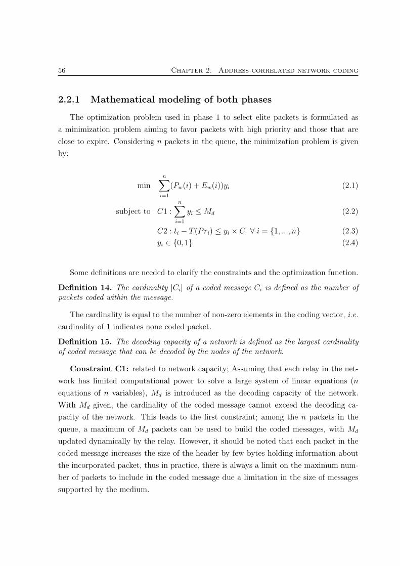
56 Chapter 2. Address correlated network coding
2.2.1 Mathematical modeling of both phases
The optimization problem used in phase 1 to select elite packets is formulated asa minimization problem aiming to favor packets with high priority and those that areclose to expire. Considering n packets in the queue, the minimization problem is givenby:
minn∑
i=1
(Pw(i) + Ew(i))yi (2.1)
subject to C1 :n∑
i=1
yi ≤Md (2.2)
C2 : ti − T (Pri) ≤ yi × C ∀ i = {1, ..., n} (2.3)yi ∈ {0, 1} (2.4)
Some definitions are needed to clarify the constraints and the optimization function.
Definition 14. The cardinality |Ci| of a coded message Ci is defined as the number ofpackets coded within the message.
The cardinality is equal to the number of non-zero elements in the coding vector, i.e.cardinality of 1 indicates none coded packet.
Definition 15. The decoding capacity of a network is defined as the largest cardinalityof coded message that can be decoded by the nodes of the network.
Constraint C1: related to network capacity; Assuming that each relay in the net-work has limited computational power to solve a large system of linear equations (nequations of n variables), Md is introduced as the decoding capacity of the network.With Md given, the cardinality of the coded message cannot exceed the decoding ca-pacity of the network. This leads to the first constraint; among the n packets in thequeue, a maximum of Md packets can be used to build the coded messages, with Md
updated dynamically by the relay. However, it should be noted that each packet in thecoded message increases the size of the header by few bytes holding information aboutthe incorporated packet, thus in practice, there is always a limit on the maximum num-ber of packets to include in the coded message due a limitation in the size of messagessupported by the medium.

2.2. ACNC: Model and definitions 57
Constraint C2: this constraint is related to priority management; given that eachpacket has a priority Pri, let T (Pri) be the maximum delay allowed for packet i. Apacket should be considered in a transmitted state at or before its maximum allowedtime, that is, when the time ti spent in the queue reaches the maximum delay T (Pri).
The objective of constraint C2 is to force the selection of expired packets.
if ti ≤ T (Pri) ⇒ ti − T (Pri) ≤ 0 yi can be 0 or 1if ti > T (Pri) ⇒ ti − T (Pri) > 0 yi should be 1
The constant C should be chosen large enough to guarantee the validity of theconstraint when ti − T (Pri) exceeds 1. Under this form, constraint C2 is fair enoughto select packets that are required to be coded and removed from the relay. However,some factors should be taken into consideration to improve constraint C2:
1. Detecting packets that are about to be late, not only those that are late.
2. Taking into consideration the time needed for a coded message, that includes lateor about to be late packets to travel to the next relay.
Therefore, T (Pri) is defined as follow:
T : R −→ RPri 7−→ F (Pri)− Pr − td
Where F (Pri) is the maximum time the packet can spend in the queue, Pr is aprecautionary constant and td the transmission delay to the next relay. td is determineddynamically depending on the network feedback and the round trip computation betweenthe relay and its neighbors.
Objective function: the objective of phase 1 model, as indicated earlier, is toincrease the amount of information in the coded message. The objective function takesinto consideration the following properties:
• Priority : two packets i and j having priorities Pri and Prj respectively with Pri <
Prj but ti − T (Pri) = tj − T (Prj) are treated equally by constraint C2 with noconsideration to their priorities.
• Expiry : two packets i and j having priorities Pri and Prj respectively with Pri = Prj
and ti−T (Pri) < tj−T (Prj) but both giving a negative left hand side of constraintC2 are treated equally by constraint C2.

58 Chapter 2. Address correlated network coding
Recall that Pri is used as the priority of packet i where priorities are between 1and H with H indicating the highest priority. The priority weight for packet i is set asfollow:
Pw(i) = −Pri (2.5)
Given formulation (2.5), the lowest weight indicates highest priority. Similarly, theexpiry weight of packet i is written as:
Ew(i) = T (Pri)− Prd − td − ti (2.6)
Formulation (2.6) indicates that the closer a packet to timeout is, the smaller thevalue of Ew(i) is. Reaching a negative value, Ew(i) indicates that packet i is delayed.
When phase 1 completes, packets are divided into two sets:
- P1 the set of packets already selected,
- P2 the set of candidate packets.
The optimization problem used for phase 2 is formulated as a maximization problemaiming to find, among unselected packets the best matching with elite packets in orderto maximize address correlation between selected packets thus reducing the number oftransmitted coded messages. The formulation of the maximization problem is given in(2.7).
maxn∑
i=1
yi (2.7)
subject to C1 :n∑
i=1
yi ≤Md (2.8)
C3 :n∑
i=1
min(1, |Sj −Di| × yiyj) <n∑
i=1
yi ∀j (2.9)
C4 :n∑
i=1
min(1, |Crj − Cri| × yiyj) <n∑
i=1
yi ∀j (2.10)
yi ∈ {0, 1} (2.11)

2.2. ACNC: Model and definitions 59
The objective of phase 2 is to complement the set of selected packets P1 by selectingsome packets from the set P2 to maximize the cardinality of the produced coded mes-sages. As done in phase 1, the solution should favor correlation between selected packetswhile maintaining the constraints on network capacity (see definition 1).
Constraint C3: this constraint is related to source/destination matching; selectedpackets should have correlated source and destination addresses so that they can becoded together and thus reducing the number of transmissions. If possible, for eachselected packet, another packet should be selected with correlated addresses. We denoteby Si and Di the source and destination of packet i and we say that two packets i andj have correlated addresses if |Sj −Di| × yiyj = 0. That is, either they are not selectedby the system (yiyj = 0) or that the source of packet i matches with the destination ofpacket j (Sj −Di = 0).
For a packet j, the left hand side of the constraint computes the number of non-matching packets with j. If the computed number is less than the number of packets,then the constraint guarantees the presence of at least one match for packet j.
Constraint C4: other criteria might be required to allow packets to be codedtogether. Constraint C3 is generalized to support any grouping criteria (other thanaddress correlation) between selected packets. Denoting by Cri the criteria of packet i,constraint C4 guarantees, to a certain level, the selection of pairs of packets with thesame criteria. The right hand side of the constraint can be replaced by ≤ 0 if all selectedpackets are required to have the same criterion.
2.2.2 Complexity analysis of the proposed model
The proposed model for phase 1 adopts a binary integer programming (BIP) model.In such a model, each decision is represented with a binary variable: setting the variableequal to 1 corresponds to making the "yes" decision, i.e. the corresponding packet isselected for coding, while setting it to 0 corresponds to the "no" decision, i.e. the cor-responding packet is not selected for coding. Constraints are then formed to correspondto the effects of the decision. Computer codes for BIP algorithm are now commonlyavailable in mathematical programming software packages. Traditionally these algo-rithms have been based on branch and bound B&B technique and its variation [46].The field of BIP has witnessed remarkable improvements over recent years. Two of the

60 Chapter 2. Address correlated network coding
biggest contributors have been heuristics [47] and parallelism [48]. The main sourceof parallelism is the fact that different nodes in the BIP search tree can be processedindependently. Given the tradeoff between speed and hardware cost, the parallelismtechnique requires powerful hardware and high energy consumption. On the other hand,the proposed model for phase 2 is a nonlinear optimization problem with linear objectivefunction. These types of problems are generally classified as NP-Hard (non-deterministicpolynomial-time hard). In real time applications, there is a need to replace traditionalmethods by iterative algorithms able to improve the performance and runs within areasonable amount of time to find a solution.
2.2.3 Low cost algorithm
In this section, a low cost iterative algorithm is presented. The algorithm has thesame objectives as the models proposed in Section 2.2.1.• Improve throughput with NC.• Improve QoS with the selection of packets to be coded.
Our low cost algorithm using network coding (LCANC) is listed in Algorithm 1. LCANCtargets packets that are about to expire to match them together. If no match is found,the algorithm uses the remaining available time to match the selected packets with non-expired packets if available. No transmission of non-coded packets occurs unless a packetexpire and cannot be matched with any other packet in the queue.
The LCANC is compared with a traditional version of NC (TNC) listed in Algorithm2. TNC does not take into consideration QoS and performs coding between the packetin the top of the queue and the first existing match in the queue. If no match is foundthe packet is transmitted individually.
2.2.4 Simulation results
To validate the efficiency of the proposed approach, a small network made of twolinear networks, A, IN1, IN2, IN5, C and B, IN3, IN2, IN4, D is implemented as shownin Figure 2.4. In this network, 4 users are exchanging different types of data such asvideo conferences, voice and file download. The simulation is done to test the globalqueuing system of the relay IN2. Packets arrive to the relay following a stochasticprobability distribution and are stored in a buffer. Considering that this buffer has a

2.2. ACNC: Model and definitions 61
Algorithm 1 LCANC1: repeat2: repeat3: Pick one packet from expired4: if matched with expired then5: Use NC6: else7: if matched with nonexpired then8: Use NC9: else
10: Send individual11: end if12: end if13: until no Expired or network capacity reached14: repeat15: Pick one packet from nonexpired16: if matched with nonexpired then17: Use NC18: end if19: until Expired or network capacity reached20: until Network stop
Algorithm 2 TNC1: repeat2: repeat3: Pick first packet from the queue4: if expired then5: Send individual6: else7: if another packet in the queue then8: if Correlation between addresses then9: Use NC
10: else11: Send individual12: end if13: end if14: end if15: until Network capacity reached16: until Network stop

62 Chapter 2. Address correlated network coding
Figure 2.4: Two linear networks intersecting at relay IN2
limited size, selecting packets from this buffer is done according to three techniques thatwill be listed shortly. Some of the selected packets are coded together; others are sentindividually. Selected packets (coded and non-coded ones) are then sent to the outputinterface. The output interface has a limited capacity that is set equal to the capacity ofthe network. This capacity is made variable to simulate the network congestion. Threealgorithms are used in our simulation to forward packets. The first algorithm considersthe traditional store and forward (SF). The second algorithm is the TNC and the thirdalgorithm is the proposed LCANC.
The performance of SF, TNC and LCANC in terms of the number of transmissionsare plotted in Figure 2.5. The network has a capacity of 8 packets. It is clear that TNChas a higher rate of transmitted packets compared to traditional store and forward. Asdescribed earlier, TNC guarantees decoding at the end user since packets are coded asfunction of some packets available at the end users. The figure shows that, using TNC,the throughput is enhanced and the number of transmitted packets exceeds the networkcapacity. Recall that network capacity is defined as the amount of data that a networkcan carry, with NC, each coded message holds multiple packets making it possible toexceed the network capacity. When the plot reaches values above SF, TNC shows thatcoding is done and that throughput gain occurs. Being below SF means that the queueat the output is not at its capacity and that the switch has fewer packets to send than thecapacity of the network allows. The major gain in throughput is observed for LCANCthat remains always above SF and TNC indicating that the algorithm always uses its

2.2. ACNC: Model and definitions 63
0 100 200 300 400 500 6000
2
4
6
8
10
12
14
Time in milliseconds
Num
ber
of p
acke
ts
SFTNCLCANC
Figure 2.5: Instantaneous number of transmitted packets
0 100 200 300 400 500 6000
200
400
600
800
1000
1200
1400
1600
Time in milliseconds
Cum
ulat
ive
num
ber
of p
acke
ts
SFTNCLCANC
Figure 2.6: Cumulative number of packets transmitted

64 Chapter 2. Address correlated network coding
0 100 200 300 400 500 600−2
0
2
4
6
8
10
12
Time in milliseconds
Num
ber
of p
acke
ts
SFTNCLCANC
Figure 2.7: Instantaneous number of delayed packets in thequeue
coding capacity to code as much packets as possible.Figure 2.6 shows the cumulative number of packets sent with respect to the time
in milliseconds. The cumulative number of packets at time t is defined as the totalnumber of packets transmitted by all the nodes of the network since the beginning ofthe simulation until time t. It is clear that for a specific time, the number of packets sentby the proposed LCANC algorithm is larger than the number of packets sent by anyother method. However, this comes at the cost of increasing the processing capabilityof the switch which is a fair compromise with respect to the throughput improvementachieved.
Figure 2.7 shows the number of packets that are delayed with each algorithm. Apacket is considered to be delayed if the time spent in the queue exceeds the maximumallowed. While SF plot shows that after a while, all packets in the network are delayed,the proposed method shows that no delayed packets are transmitted. This proves thatthe proposed method manages the selection of candidate packets to be coded in anefficient way.

2.3. A practical implementation of ACNC 65
2.3 A practical implementation of ACNC
ACNC adds a layer between the data link and the network layers of the OSI net-working model. In general, ACNC generates a coded message made of packets codedtogether using XOR operation on bits of the packets. A header is added to each codedmessage describing each packet coded within the message and the correlation betweenthese packets. ACNC also uses adaptive flag to steer coded messages to various desti-nations. Adaptive parameters are used in [49] where NC is employed only for packetsbelonging to the same generation. In their work, feedback from the receivers to thesource is used to adaptively adjust the generation size and thus maximize the numberof packets successfully decoded at the receivers. In this section, we detail the process ofreceiving, coding and forwarding messages using ACNC.
2.3.1 Context and network
We work in the context where a switch (or an intermediate node) receives packetsand coded messages that need to be forwarded to their destinations. Our receiving,coding and forwarding process (RCFP) is used whenever the node receives or has inits queue, potential messages to code and transmit. RCFP in fact is divided into twoparts; receiving process (RP) which is used to handle received messages and immediatelyupdates the corresponding adaptive flag, and the coding and forwarding process (CFP)that uses the updated adaptive flag to code and transmit messages. RP/CFP protocolis placed between the Data Link and the network layer in the communication layeringstack.
2.3.2 Receiving, coding and forwarding process
The process of coding and forwarding messages requires adding a header to thecreated coded messages. This header allows receiving nodes to identify packets includedin the coded message and consequently route copies of the coded messages to variousdestinations. The receiving, coding and forwarding process is described in this section.

66 Chapter 2. Address correlated network coding
?��
��Start
?A new message
arrives
?
����
HHHH����
HHHHBroadcasted?
?
N
-Y
����
����Algorithm:
Check if concerned
����
HHHH����
HHHHConcerned?
?
N
Discard
�
?Y�
����
HHHH����
HHHHCoded?
N
-
?Y
����
����Algorithm:
Adjust adaptive flag
?Send to queue
?��
��Stop
Figure 2.8: Receiving Process (RP)
Receiving process (RP)
A node can receive coded or uncoded messages. If a message is received by the nodein a broadcast mode, the node needs to check whether it is concerned or not by thatmessage. A node is concerned by a message if it is either the destination of the message(i.e. the destination of at least one of the coded packets in the message) or if it is arelay on the path from the source to the destination of one of the packets coded in themessage. If the node is concerned by the received message, it immediately updates theadaptive flag of the received message and sends it for queuing. The receiving process ispresented in Figure 2.8.

2.3. A practical implementation of ACNC 67
Coding and Forwarding Process (CFP)
An intermediate node might decide to forward a received message or to code messagestogether in order to improve throughput. The decision is based on QoS constraints asdescribed in section 2.2. The first step in CFP is to validate the capability of end usersto decode each message. Capability of decoding is validated using adaptive flag. Oncethe possibility of decoding is confirmed, CFP performs a coding process and creates acoded message. The coded message is prefixed by a header that describes each packetincluded in the coded message and holds the corresponding adaptive flag. The messageis then transmitted to the network. The overall CFP process is presented in Figure 2.9.
?��
��Start
?Two
messagesto code
?
��
��
@@
@@
��
��
@@
@@At least
one is codedmessage?
?
N
-Y
����
����Algorithm:
Validate decodability
����
HHHH����
HHHHDecodable?
?
N
Reject
�
?Y�
Code messagesand
build the header
?
����
����Algorithm:
Adjust adaptive flag
?Transmit
Unicast or Broadcast
?��
��Stop
Figure 2.9: Coding and Forwarding Process (CFP)

68 Chapter 2. Address correlated network coding
Table 2.1: Message header
Unicast Tells if the message is a unicast of a broadcastAddr1 All packets in the coded message have Addr1 (respectively Addr2)Addr2 as origin and Addr2 (respectively Addr1) as destinationComing from The neighboring node sending the messageNb. of packets Number of packets coded inside the messageID Identification of the packetSource Origin or source of the packetExist at dest. Adaptive flag that tells if the packet exists at destinationNext hop Neighboring node on the path to destination
2.3.3 Message header
The header of a message is shown in Table 2.1. The first part of the header describesthe coded message, which indicates that it is exchanged between end nodes identified byAddr1 and Addr2 and released by node "Coming from". Note that Addr1 and Addr2 arethe correlated addresses and can be interchanged . The other part describes the packetscoded together and is repeated as many times as there are packets in the coded message.Each section lists four important characteristics of the packet; its ID, its source node, theadaptive flag "Exist at dest." which indicates whether the packet exists at destinationor not and the next hop of the packet. The header is updated each time the codedmessage reaches an intermediate node and each time it is coded with another message.The coding of different types of messages together and the update of the adaptive flag isdetailed in subsequent sections. We then describe the forwarding and receiving processesand the usage of the adaptive flag to guide the messages to its destinations.
2.3.4 Coding two packets
Switch INi decides to code two packets as described in Table 2.2. These packets arereceived from neighboring nodes as shown in Figure 2.10
Packets 123 and 124 are XORed together to form a new coded message that will betransmitted from switch. The header of the coded message is listed in Table 2.3a.
After building the coded message, fields such unicast, "Exist at destination" andnext hop needs to be updated. Next hop is determined by looking at the routing tableof the node. The next hop of packet 123 is INi+1 and the next hop of packet 124 is
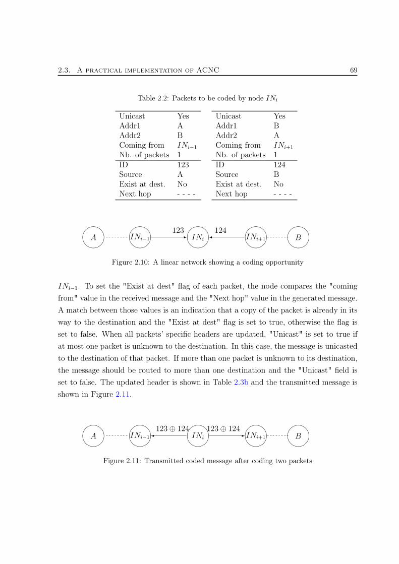
2.3. A practical implementation of ACNC 69
Table 2.2: Packets to be coded by node INi
Unicast YesAddr1 AAddr2 BComing from INi−1
Nb. of packets 1ID 123Source AExist at dest. NoNext hop - - - -
Unicast YesAddr1 BAddr2 AComing from INi+1
Nb. of packets 1ID 124Source BExist at dest. NoNext hop - - - -
����A ��
��INi−1
-123
����INi
�124
����INi+1 ��
��B
Figure 2.10: A linear network showing a coding opportunity
INi−1. To set the "Exist at dest" flag of each packet, the node compares the "comingfrom" value in the received message and the "Next hop" value in the generated message.A match between those values is an indication that a copy of the packet is already in itsway to the destination and the "Exist at dest" flag is set to true, otherwise the flag isset to false. When all packets’ specific headers are updated, "Unicast" is set to true ifat most one packet is unknown to the destination. In this case, the message is unicastedto the destination of that packet. If more than one packet is unknown to its destination,the message should be routed to more than one destination and the "Unicast" field isset to false. The updated header is shown in Table 2.3b and the transmitted message isshown in Figure 2.11.
����A ��
��INi−1
�123⊕ 124
����INi
-123⊕ 124
����INi+1 ��
��B
Figure 2.11: Transmitted coded message after coding two packets

70 Chapter 2. Address correlated network coding
Table 2.3: New created coded message
(a) New header of a coded message creating bycoding two packets
Unicast - - -Addr1 AAddr2 BComing from INi
Nb. of packets 2ID 123Source AExist at dest. - - - -Next hop - - - -ID 124Source BExist at dest. - - - -Next hop - - - -
(b) Updated header of the coded message beforetransmission
Unicast NoAddr1 AAddr2 BComing from INi
Nb. of packets 2ID 123Source AExist at dest. NoNext hop INi+1
ID 124Source BExist at dest. NoNext hop INi−1
2.3.5 Receiving a message by unconcerned node
When node INj receives a broadcasted coded message it performs Algorithm 3 totest whether it is concerned or not by that message. The intermediate node is concernedby a message if it is the next hop of any of the packets contained in the message.
Algorithm 3 Test if concerned node1: loop on all packets in the message2: if Next hop = INj then3: Set to Concerned4: Stop5: end if6: end loop7: Discard the message
2.3.6 Receiving coded message by concerned node
When node INi+1 receives a broadcasted coded message and it is a concerned node(one of the next hops is indeed IN i+1). It performs Algorithm 4 to update the headerinformation of the received node. In line 4 of Algorithm 4, the "Exist at dest." is set to

2.3. A practical implementation of ACNC 71
true when a packet is coming from a node considered in the routing table as the nexthop of the packet in its way to destination.
Algorithm 4 Update adaptive flag1: loop on all packets in the message2: NH ←− next hop according to routing tables3: if NH = Coming From then4: Exist at Dest. ←− Yes5: else6: Set next hop7: end if8: end loop
2.3.7 Update of the flag "Exist at Dest."
A coded message is created and broadcasted by node INi+1 after coding packets 224received from INi and 225 received from IN i+2. Node INi decides to code a packet witha the coded message. When node INi receives the broadcasted coded message it runsAlgorithm 4 to update its header information including adaptive flag. The context ofthe transmission is shown in Figure 2.12 and the headers are shown in Table 2.4.
����A ��
��INi−1
-223
����INi
�224⊕ 225
����INi+1 ��
��B
Figure 2.12: Coding one packet and one coded message
Coding feasibility
Before presenting the coding scheme, the coding node should validate the decodingfeasibility of the resulting message at each destination. Referring to Table 2.4, thepossibility of coding is justified as follows; end node A has messages 223, 225 and missingmessage 224 while end node B has messages 224, 225 and missing 223.

72 Chapter 2. Address correlated network coding
Table 2.4: A packet and a coded message to be coded by node INi
Unicast yesAddr1 AAddr2 BComing from INi−1
Nb. of packets 1ID 223Source AExist at dest. NoNext hop INi
Unicast YesAddr1 AAddr2 BComing from INi+1
Nb. of packets 2ID 225Source AExist at dest. YesNext hop INi+2
ID 224Source BExist at dest. NoNext hop INi
Algorithm to test coding feasibility
When selecting messages to code, the switch needs to check the feasibility of decodingthe resulting coded message at end nodes. It is possible to decode a message at any endnode if the number of unknown packets contained in the coded message is at most one.Moreover, given the characteristic of the XOR operation it is unfeasible to code twomessages together if they both contain the same packet with the flag "Exist at Dest."set to false since the packet might vanish from the network without being delivered.Algorithm 5 is performed to check the feasibility of coding messages together.
Coding before transmission
The three packets 223, 224 and 225 are XORed together to form a new coded message.The header of the created message is shown in Table 2.5 and the message is broadcastedinto the network. The case of combining two coded messages can easily be deduced andwill not be detailed here.
2.3.8 Decoding process
The decoding process can occur at end nodes (centralized approach) or at interme-diate nodes (distributed approach). Decoding requires both buffering and computation.Buffers are needed to keep copies of sent and received packets that are needed later in

2.3. A practical implementation of ACNC 73
Algorithm 5 Testing Coding Feasibility1: loop on each packet i in the coded message header2: Count← 03: loop on every packet P in every message to code4: if Source of P̸= i and Exist at Dest. = No then5: if similar packet with Exist at Dest. = No
ORno similar packet exists then
6: Count← Count+ 17: end if8: end if9: end loop
10: if Count > 1 then11: Set Coding to unfeasible12: Stop13: end if14: end loop15: Set Coding to feasible
the decoding process. Decoding itself is not straightforward. The decoding node shouldXOR the received message with every buffered packet that is part of the coded message.In this thesis, we study the advantages and disadvantages of both approaches.
2.3.9 Simulation results
We ran our simulation on a network of 5 nodes, A, IN1, IN2, IN3 and B. In thisnetwork, both sources A and B are exchanging packets at the same rate on a static link.The system is synchronized in the sense that all nodes transmit at the same time. Weconsider also two channel use on each link. The objective of the simulation is to measurethe cardinality (i.e. the number of packets) of the coded messages released by differentnodes. Figure 2.13 shows the cardinality of coded messages released by A, and thecardinality of coded messages released by IN1 and IN2. It is important to note that thecardinality of the coded messages remain low due to two facts, first the XOR operationthat eliminates duplicated packets and second, the fact that the network activities aresynchronized.
In a second time, the synchronization of the system is removed and the transmissionat each node is a stochastic process, where each node has a certain probability to trans-

74 Chapter 2. Address correlated network coding
Table 2.5: Header of created coded message
Unicast NoAddr1 AAddr2 BComing from INi
Nb. of packets 3ID 223Source AExist at dest. NoNext hop INi+1
ID 224Source BExist at dest. NoNext hop INi−1
ID 225Source AExist at dest. YesNext hop INi−1
mit its coded message. With a probability of 0.75%, Figure 2.14 shows the cardinalityof the coded messages at A, IN1 and IN2. This simulation shows that the cardinality iscontinuously increasing and requires further study of the behavior of the system. Notethat the behavior of the cardinality remains similar for different transmission probabili-ties.
2.4 Relay correlated network coding
The address correlated NC can be extended to relay correlated network coding(RCNC). Consider the network illustrated in Figure 2.15 where A is sending a file to B
and C is sending a file to D. With address correlated NC, no saving on the bandwidthcan occur since no address correlated packets exist among the flow on intermediate nodesni; i = 1 to 4. However, if address correlated NC is applied between relays n1 and n4
then a considerable saving on the bandwidth can be made due to the presence of correla-tion in the flow between n1 and n4. The RCNC is not only theoretical. Current networksarchitecture makes the use of RCNC feasible and practical. Most networks connected to

2.4. Relay correlated network coding 75
0 10 20 30 40 500
0.5
1
1.5
2
2.5
3
Transmissions
Car
dina
lity
AIN
1
IN2
Figure 2.13: Cardinality of coded message at different nodes
0 10 20 30 40 500
5
10
15
20
25
30
35
40
Transmissions
Car
dina
lity
AIN
1
IN2
Figure 2.14: Cardinality of coded message at different nodeswithout synchronization

76 Chapter 2. Address correlated network coding
Figure 2.15: Example of networks where RCNC can be used
the Internet are based on the TCP/IP stack where IP version 4 is implemented. Eachdevice on the internet has a unique IP address made of 32 bits. Due to the large numberof devices connected to the Internet, a 32 bit field is not enough to connect every deviceon the globe. IP version 4 offers a solution identified as network address translation or(NAT).
With NAT, all local area networks (LAN) use private IP. The gateway routers per-form NAT to translate the private IP to a public IP allowed to travel on the Internet.With this mechanism, the number of possible devices connected to the Internet exceedsthe capacity of the 32-bit IP field. With NAT, packets traveling through the publicnetwork are seen as packets exchanged between gateway routers. In such case a massexchange between two networks is relay correlated and RCNC can be applied to save onbandwidth. With IPv6 the concept of public / private IP is not clear. Private IPs existin IPv6 (prefixed with 0xFD) but NAT translation is not, or at least to be avoided.
2.5 Conclusion
In this chapter, we introduced address correlated NC as a new protocol that en-hances bandwidth usage when two nodes are exchanging information. We demonstratedthat with the use of adaptive flag, we are able to achieve throughput gain with NCby performing simple algorithms to guarantee decodability at end nodes. With ACNC,intermediate nodes perform only coding operations and route messages to multiple des-tinations. Contrary to other NC protocols, decoding is only performed at end nodeswhere new messages are extracted from every received coded message. Consequently,

2.5. Conclusion 77
we are able with ACNC, to route coded messages to their intended destinations using aspecific routing mechanism also based on adaptive flag.
We then provided a new packet selection process. For this process, we proposed anoptimization model that takes into consideration throughput improvement by forcing theselection of address correlated packets, and delay management by forcing the selectionof delayed packets. We then proposed a low cost algorithm based on address correlationto efficiently select packets to be coded and released into the network. The algorithmnot only improves bandwidth where the number of received packets is larger than thenumber of transmitted ones, but it also guarantees a certain level of QoS by managingdelays and priority of packets. At last, the study investigated in this chapter has beenaccepted in two international conferences, IWCMC [C3] and ICCIT [C4].


CHAPTER
3 Centralized decoding
In Chapter 2, we proposed the ACNC algorithm and clarified the coding and thedecoding processes. In this chapter, we detail the centralized decoding approach whereintermediate nodes are responsible for seizing coding opportunities to code messagestogether in order to reduce bandwidth utilization, and end nodes are responsible fordecoding. This process requires significant buffering capability and increases the com-putation complexity at end nodes. However, no overhead is added to intermediate nodeswhere only coding algorithms are implemented.
In this chapter, we study ACNC at both intermediate and end nodes. The contribu-tion of this chapter is of several folds. First, we present a decision model at nodes thatbalances between the receiving and the sending queues. Second, we present the codinggraph, a new technique that helps counting the number of transmissions and codingopportunities when ACNC is used on linear networks. At intermediate nodes, we studythe coding opportunities and analyze the size, byte overhead and information contentsof coded messages. Third, we study the buffering requirements at end nodes, and thecomplexity needed for decoding and finally, we set a maturity restriction on packets inthe network to prevent packets to live forever in coded messages.
3.1 Decision models for centralized decoding
In this thesis, the considered network consists of nodes that implement a servermanaging two queues as shown in Figure 3.1; the receiving queue and the outgoingqueue. The receiving queue is used to store all received messages and has a capacitydenoted byCrq . We also denote by xrq(t) the number of messages at time t waitingin the receiving queue. The server investigates the collected messages in the receivingqueue to search for coding opportunities on address correlated packets which are onlyallowed to be coded together. Coded messages are then transferred to the outgoingqueue. Therefore, the outgoing queue holds messages ready to be transmitted to thenetwork. We denote by Coq and xoq(t) the capacity and the number of coded messages
79

80 Chapter 3. Centralized decoding
Figure 3.1: Node model
at time t in the outgoing queue respectively. The presence of two queues facilitates thescheduling task at the node and reduces the time needed to search for matching messagesto be coded.
The server mainly performs one of the following activities:- Packet generation denoted by g
- Coding activity denoted by c
- Sending message denoted by s
- Decoding activity denoted by d
The assignment of activities to nodes is completed according to the node role asdescribed in the following scheme:
- Sending node activity set = {g, s}- Intermediate node activity set = {c, s}- Receiving node activity set = {d}Note that, when a network node plays more than one role, its set of activity is the
union of the activity set associated to each role. For example, the set of activities atan end node is {g, s, d}. At time t, each node selects an activity to perform from itsactivity set. A decision model is needed at each node to select the best activity. Twodecision models are adopted for our implementation, a deterministic decision model forintermediate nodes and a probabilistic model for end nodes.
State diagram at intermediate nodes
Intermediate nodes are responsible for coding and sending messages. The state di-agram of an intermediate node is shown in Figure 3.2. In this diagram, the codingphase is represented by a link from the receiving queue to the server where two or moremessages are selected from the receiving queue to be coded together and sent to theoutgoing queue. Note that some messages might be transferred from the receiving to

3.1. Decision models for centralized decoding 81
Figure 3.2: Intermediate node state diagram
outgoing queue without being coded, this happens to preserve QoS. The transmissionphase is represented by a link from the outgoing queue to the server where one messageis transmitted by the server to neighboring nodes. Note that the coding activity includesupdating message headers according to the routing table at each node.
State diagram at end nodes
Similarly, the state diagram of an end node is shown in Figure 3.3. In this diagram,the decoding phase is represented by a link between the receiving queue and the serverwhere one message is selected to be decoded and transferred eventually to upper layer. Amessage containing several packets can be decoded if a maximum of one of these packetsdoes not exist at destination. If the server is unable to decode a message, the messageis returned to the receiving queue and further retries are performed later when morereceived packets are available. The generation phase is represented by a link betweenthe server and the outgoing queue and packets are generated according to a model thatwill be described later. Finally, the transmission phase is represented by a link from theoutgoing queue to the server where one message is transmitted to neighboring nodes.
3.1.1 Deterministic model for intermediate nodes
At intermediate nodes, the decision fluctuates between coding and sending messagesand the selection of the activity to be performed largely depends on the number ofmessages in the queues. The decision model needs to constantly balance the occupationof both receiving and outgoing queues. When balanced, the decision model preservesQoS and favors early received messages in both queues to be processed. For that purpose,

82 Chapter 3. Centralized decoding
Figure 3.3: End node state diagram
an integer programming problem is proposed where a binary variable yi, i ∈ {c, s} isassigned to each possible activity. yi is 0 if the activity is not performed and 1 elsewhere.The model is shown as follows:
max yc(t)
xr(t)∑i=1
mri(t) + ys(t)xo∑i=1
moi(t) (3.1)
subject to yc(t) + ys(t) = 1 (3.2)
yc(t) ≥(xr(t)− xo(t))− dro
Cr
(3.3)
ys(t) ≥(xo(t)− xr(t))− dor
Co
(3.4)
yc, ys ∈ {0, 1} (3.5)
In this problem, dro (respectively dor) is the acceptable difference in number of mes-sages between the receiving and outgoing queues (respectively between the outgoing andreceiving queues), and mri(t) is the amount of time message i has been in the receivingqueue while moj(t) is the amount of time message j has been in the outgoing queue.
The constraint (3.3) forces yc(t) to be 1 whenever the difference between the numberof messages waiting to be further coded xr(t) and the number of messages waiting tobe transmitted xo(t) reaches or exceeds the value dro . In this case, the right hand sideof (3.3) is strictly positive forcing yc(t) to take a non zero value. Similar objective canbe found for (3.4) by forcing ys(t) to be 1 when the difference between the number

3.1. Decision models for centralized decoding 83
of messages waiting to be transmitted xo(t) and the number of messages waiting tobe further coded (xr(t)) reaches or exceeds dro . The values Cr and Co are selected tobe large enough so that the right hand sides of both (3.3) and (3.4) do not exceed 1.Equation (3.2) guarantees that the server performs exactly one task at a time. It shouldbe noted that (3.3) and (3.4) are built to guarantee that only one of the binary variablesyc(t) and ys(t) is forced to be 1, however, both variables are allowed be 0 at the sametime which explains the need for (3.2).
When the load of both queues is balanced, both binary variables are unrestricted bythe constraints of the model and (yc, ys) is chosen in order to maximize (3.1). Naturally,the choice forces the release of messages waiting for a longtime in the queues.
3.1.2 Probabilistic model for end nodes
At end nodes, a binary variable yi, i ∈ {d, g, s} is assigned to each possible activity.yi is 0 if the activity is not performed and 1 otherwise. As for the case of intermediatenodes, the server can perform exactly one task at a time. We denote by P (d), P (g) andP (s) respectively the decoding, generation and sending probabilities.
The packet generation is considered as an independent event from other activitieswhere the decision of the activity to be undertaken at end nodes is performed in twophases. During the first phase, a decision is taken on whether or not the node shouldgenerate a packet. If no packet is to be generated, we move to the second phase to select,according to a stochastic decision model, the node activity to be performed.
The stochastic decision is based on the model proposed in [50] where packets routingis described by probabilistic functions depending on the application. For our case, weuse the following equations:
P (d) =e−βxoq(t)
e−βxoq(t) + e−βxrq(t)(3.6)
P (s) =e−βxrq(t)
e−βxoq(t) + e−βxrq(t)(3.7)
Where β is a control parameter and P (d) +P (s) = 1 . In (3.6) decoding probabilitydecreases when the number of messages in the outgoing queue increases favoring in thiscase the sending activity, and a similar argument can be given to (3.7). However, evenwhen the number of coded messages in the outgoing queue (respectively receiving queue)

84 Chapter 3. Centralized decoding
exceeds the number of coded messages in the receiving queue (respectively outgoingqueue), there is still a non zero probability to select decoding (respectively sending)activity.
As noted in [50], if we set β = 0, both probabilities are equal to 1/2 and decoding orsending are chosen randomly. On the other hand, if β grows to infinite, limβ→∞ P (d) = 0
and limβ→∞ P (s) = 1 when xoq(t) > xrq(t) thus creating a deterministic decision modelwhere the activity is selected according to queues occupation.
To argue the usage of a probabilistic model at end nodes we consider the followingfacts:
- The generation of packets is an application activity considered as a random process.- Contrary to intermediate nodes, end nodes are not completely dedicated for net-
work activities, and the generation of packets is a stochastic process.
3.1.3 Activity selection algorithms
Models presented in Sections 3.1.2 and 3.1.1 are used to propose two low cost algo-rithms to select the best activity at intermediate nodes and at end nodes respectively.These algorithms are initiated each time the node has to take a decision. The activityselection scheme is detailed in Algorithm 6.
In this algorithm, steps 1 and 3 represent constraints (3.3) and (3.4) in the optimiza-tion problem presented in (3.1) and select the activity to be performed depending onthe occupation of the receiving and outgoing queues. When queues are almost balanced,steps from 6 to 17 attempt to maximize (3.1) helping late packets to be released fromthe queues and improving QoS.
The decision model algorithm at end nodes is presented in Algorithm 7. In thisalgorithm, step 2 independently selects the generation activity with a certain predefinedprobability. If no new packets are generated, the code between lines 5 and 10 giveshigher probability to the activity that balances the receiving and outgoing queues.
3.2 Study of coding and decoding activities
In this section, we closely study the centralized decoding from different points ofview. Initially, we plot the coding activities through intermediate nodes and investigate
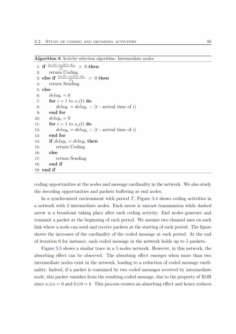
3.2. Study of coding and decoding activities 85
Algorithm 6 Activity selection algorithm: Intermediate nodes
1: if (xr(t)−xo(t))−droCr
> 0 then2: return Coding3: else if (xo(t)−xr(t))−dor
Co> 0 then
4: return Sending5: else6: delayr = 07: for i = 1 to xr(t) do8: delayr = delayr + (t - arrival time of i)9: end for
10: delayo = 011: for i = 1 to xo(t) do12: delayo = delayo + (t - arrival time of i)13: end for14: if delayr > delayo then15: return Coding16: else17: return Sending18: end if19: end if
coding opportunities at the nodes and message cardinality in the network. We also studythe decoding opportunities and packets buffering at end nodes.
In a synchronized environment with period T , Figure 3.4 shows coding activities ina network with 2 intermediate nodes. Each arrow is unicast transmission while dashedarrow is a broadcast taking place after each coding activity. End nodes generate andtransmit a packet at the beginning of each period. We assume two channel uses on eachlink where a node can send and receive packets at the starting of each period. The figureshows the increases of the cardinality of the coded message at each period. At the endof iteration 6 for instance, each coded message in the network holds up to 5 packets.
Figure 3.5 shows a similar trace in a 5 nodes network. However, in this network, theabsorbing effect can be observed. The absorbing effect emerges when more than twointermediate nodes exist in the network, leading to a reduction of coded message cardi-nality. Indeed, if a packet is contained by two coded messages received by intermediatenode, this packet vanishes from the resulting coded message, due to the property of XORsince a⊕a = 0 and b⊕0 = b. This process creates an absorbing effect and hence reduces

86 Chapter 3. Centralized decoding
Figure 3.4: Coding activities in a 4 nodes network
the cardinality of coded messages. However, there is no guarantee that the architectureof the network will always favor a complete synchronization of the network activities,thus no guarantee that the network will always favor the absorbing effect.
3.2.1 Coding graph
To analytically compute the cardinality of coded messages in the network, we intro-duce the coding graph shown in Figure 3.6 and Figure 3.7 with odd and even numberof intermediate nodes respectively. Note that, in these graphs, it is assumed that thenetwork is synchronized with a time period T . Coding graphs demonstrate the cod-ing opportunity when packets are exchanged between end nodes. After coding, coded
Algorithm 7 Activity selection algorithm: End nodes
1: P (generation) = random(0, 1)2: if P (generation) <= (Generation-threshold) then3: return Generation4: end if5: P (decoding) = e−βxoq(t)
e−βxoq(t)+e−βxrq(t)
6: if P (decoding) <= random(0, 1) then7: return Decoding8: else9: return Sending
10: end if

3.2. Study of coding and decoding activities 87
Figure 3.5: Tracing coding activities in a 5 nodes network
messages are broadcasted and received by the two neighboring nodes.Arrows in the coding graph represent newly generated packets by end nodes. In
Figure 3.6 the first coding opportunity occurs at iteration 4 (top level of the graph)when the first two generated packets meet at IN4 creating the first coded message withcardinality of 2. While this coded message is broadcasted to neighboring nodes IN3
and IN5, intermediate node IN4 receives a new set of packets creating a second codedmessage with cardinality of 2. Black and gray vertices show coding opportunities withnewly created packets while white vertices show coding opportunities between codedmessages. In each of these coding graphs, two coded messages, shown in two differentcolors (i.e. black and gray), are constructed and exchanged by intermediate nodes.After a transition time, these coded messages reach the end nodes and start deliveringpackets. We notice in these figures that at each iteration, two packets are released fromthe two end nodes while an average of one packet is injected into each coded message.In fact, when the delivery process started, Figure 3.6 shows two packets added to theblack coded message every two iterations thus an average of one packet per iteration.The same occurs for the gray coded message. These coding graphs are used by Theorem2 to compute the cardinality of coded messages in the network.
Theorem 2. Given a linear network G = (N,E) with two end nodes and P packetsexchanged between end nodes (P/2 released by each end node) an upper bound on codedmessage cardinality at a given iteration i at any intermediate node in the network is

88 Chapter 3. Centralized decoding
Figure 3.6: Coding graph for 7 intermediate nodes (odd numberof nodes)
Figure 3.7: Coding graph for 6 intermediate nodes (even numberof nodes)

3.2. Study of coding and decoding activities 89
given by:
C(P,N, i) ≤ 2 min
(i,
⌈N − 2
2
⌉)+max
((min
(i,P
2
)−⌈N − 2
2
⌉), 0
)(3.8)
where N is the number of nodes in the linear network.
Proof. The first part of (3.8) counts the number of new packets added to the codedmessage at each iteration while the message is not yet delivered to the end nodes i.e.,still within the vertical bold dashed lines. In this case, the message receives two newpackets at each iteration. The number of iterations before delivering the message toan end node is
⌈N−22
⌉which is the distance between the central intermediate node IN4
and the end nodes according to Figure 3.6. The second part counts the number of newpackets added to the message after being delivered to end nodes i.e, after i >
⌈N−22
⌉. In
this case and referring also to Figure 3.6, two packets are added to the coded messageeach two iterations.
The same proof applies when the number of intermediate nodes is even. In fact, asimple linear translation of the gray nodes in Figure 3.7 leads to the structure of thecoded graph in Figure 3.6. �
Simulations are done to experimentally compute the cardinality of coded messageswithin different types of networks and at different intermediate nodes. As the size of acoded message can grow infinitely depending on the number of packets exchanged, sim-ulations are conducted on networks with an even and odd number of nodes respectively.1000 packets (500 packets transmitted from each end node) are exchanged between thetwo end nodes and results in Figure 3.8 and Figure 3.9 show the growth of the cardinalityof coded messages transmitted from selected nodes. The figures show the upper boundon the cardinality of the coded messages given in Theorem 2.
3.2.2 Buffering time
The buffering time of a packet at a node is computed as the difference between thetime the packet has started being stored at the node and the last time the packet is usedfor decoding. Figure 3.10 shows in percentage with respect to the total communicationtime, the highest and the average buffering time at each node of the network. Asshown in the figure, the buffer size at each of the end nodes should be large enough tohold all exchanged packets since the largest buffering time is almost equal to the totaltransmission time needed to deliver all the packets. This is justified by the fact that the

90 Chapter 3. Centralized decoding
0 100 200 300 400 5000
50
100
150
200
250
300
350
400
450
500C
ardi
nalit
y of
cod
ed m
essa
ges
(Pol
ynom
ial f
itted
)
Number of transmitted packets from each end node
Cardinality of messages transmitted from IN1Cardinality of messages transmitted from IN4Cardinality of messages transmitted from IN5Upper bound
Figure 3.8: Cardinality of coded messages with centralized de-coding for a network of 8 nodes
0 100 200 300 400 5000
50
100
150
200
250
300
350
400
450
500
Car
dina
lity
of c
oded
mes
sage
s (P
olyn
omia
l fitt
ed)
Number of transmitted packets from each end node
Cardinality of messages transmitted from IN1Cardinality of messages transmitted from IN4Cardinality of messages transmitted from IN5Upper bound
Figure 3.9: Cardinality of coded messages with centralized de-coding for a network of 9 nodes

3.2. Study of coding and decoding activities 91
0
10
20
30
40
50
60
70
80
90
100P
erce
ntag
e of
buf
ferin
g tim
e
Nodes in the network
45
97
00 00 00 00 00 00
45
97
A IN1
IN2
IN3
IN4
IN5
IN6
B
Average buffering timeMaximum buffering time
Figure 3.10: Decoding at end nodes: buffering time at each endnode (1000 packets exchanged in network of 8 nodes)
early generated packets might remain as part of the coded messages till the completionof the communication.
Figure 3.11 shows a polynomial fit of the buffering time in seconds of the receivedpackets at each of the end nodes. The total duration of the simulation is 5.7 seconds.This figure completes Figure 3.10 which indicates that early transmitted packets remainpart of the coded messages till the end of the communication. These packets create anoverhead in the coded message since they are already delivered and exhibit complexityand buffering overhead at end nodes. In Section 3.3, the concept of aging is introducedto remediate to this problem.
3.2.3 Byte overhead transmission
Without NC, exactly (N − 1)P transmissions are needed to exchange P packetsbetween the two end nodes of a linear network. With NC, this number is dramaticallyreduced as noticed in the coding graphs. A lower bound on the number of transmissions

92 Chapter 3. Centralized decoding
0 100 200 300 400 5000
1
2
3
4
5
6B
uffe
rrin
g tim
e in
sec
onds
(P
olyn
omia
l fitt
ed)
Received packets
Buffering time at node ABuffering time at node B
Figure 3.11: Buffering time of received packets
needed to exchange P packets is
P + (N − 2)P
2
where the first term accounts for the transmissions at the 2 end nodes and the secondterm accounts for the transmissions at the intermediate nodes when considering theoptimal case where each intermediate node is continuously performing NC operationsaving one transmission over 2. Thus, a lower bound to the total number of transmissionsequals to N × P
2.
Table 3.1: Lower bound on the number of bytes exchanged with and without NC
Protocol Transmissions Exchanged bytesTraditional store and forward (N − 1)P (N − 1)PPa (3.9)
NC-decoding at end nodes N P2
N P2Pa + Ph(N − 2)P (P+2)
8(3.10)
Denoting by Pa the size in bytes of a packet and by Ph the size of the packet header,the total number of bytes exchanged with and without NC is presented in Table 3.1.

3.3. The aging concept 93
With NC where decoding is conducted at end nodes, the cardinality of the coded mes-sages increases linearly with the number of packets transmitted, leading to an increasein the number of bytes exchanged. This increase is due to the overhead exhibited in theheader where bytes are added for each packet taking part in a coded message. Referringto Theorem 2, the size of the headers generated by the NC process is computed in bytesas (N − 2)× Ph ×
∑P2i=1 i which can also be written as (N − 2)× Ph × P (P+2)
8.
3.3 The aging concept
We consider again linear networks where end nodes exchange information synchronouslywith a time period T and two channels are available on each link between the nodes ofthe network allowing simultaneous transmissions of two messages during each time pe-riod T . The network model is represented as an undirected graph G = (N,E) wherethe set of nodes N is divided into two subsets, {A,B}, the set of end nodes and IN theset of intermediate nodes.
3.3.1 Definitions and principles
The following definitions are needed in order to describe the aging concept.
Definition 16. The age of a packet is defined as the number of times the packet con-tributes to a coded message and the age of a coded message is defined as the age of theoldest packet in the coded message.
Definition 17. The coding capacity of a network, denoted by Ç is defined as the numberof coded or uncoded messages that can be further coded together.
A coding capacity of two indicates that any released coded message from a node isthe resulting of coding at most two received messages together.
Definition 18. The diversity of a coded message is defined as the number of distinctpackets within the coded message.
Note that, when XORing is used to code messages together, diversity and cardinalitycoincide.
Definition 19. The maturity of a network is defined as the highest allowed age for allthe packets in the network.

94 Chapter 3. Centralized decoding
To prevent packet i from growing in age beyond maturity, we prevent coding oper-ations with messages containing i. For each newly generated packet i, we assign theaging variable αi initially set to 0. Each time a coded message is created with packet i,the aging parameter of that packet is incremented by 1. The age of a coded message Cj,denoted by αCj
, is calculated as follows: αCj= max(αi) ∀ i ∈ Cj. Two parameters are
set by the network and used by intermediate nodes when messages are coded together:Ç denoting the coding capacity of the nodes and µ denoting the maturity of the packets.
3.3.2 Cardinality of messages in NC
In some communication networks such as satellite networks, a single intermediatenode (relay) is used to exchange information between end nodes. The intermediate nodecodes received packets and broadcasts the coded messages back to source nodes. A simpleXORing of the received messages is enough to double the bandwidth and increase thetransmission rate [51, 52]. When the number of intermediate nodes exceeds one, codingbecomes more challenging. In this context, intermediate nodes receive not only newlygenerated packets but also coded messages that need to be further coded together.
Let us consider the network of Figure 3.4. End node A generates packets labeled1,2,3,4... While end node B generates packets labeled a, b, c, d... Intermediate nodes, i.e.IN1 and IN2 process the received packets and broadcast coded messages to neighboringnodes. Notice that packet a for example is oscillating between two intermediate nodeswithin a coded message and the cardinality of the coded message increases by one at eachiteration. The decoding of the received messages at end node A or end node B requiresthe complete buffering of all already transmitted and received packets. When a networkcontains more than two intermediate nodes, the absorbing effect emerges leading to areduction in the cardinality of coded messages. However as stated in Section 3.2, there isno guarantee that the architecture of the network will always favor the absorbing effect.
3.3.3 Aging and maturity in network coding
To prevent the cardinality of coded messages from increasing indefinitely and tomake sure that packets released into the network will vanish after a certain amount oftime, we assign an age to each packet, initially set to 0 when the packet is generatedand released by an end node. Moreover, the age of a packet is incremented each time

3.3. The aging concept 95
the packet is used as a part of a newly coded message. When a node INi receivescoded messages, it searches for matching possibilities for further coding by performingAlgorithm 8. The aging concept is shown in steps 3 and 7 to ensure that coding isprohibited when needed. The computation overhead created by the aging concept inAlgorithm 8 is hence negligible.
Algorithm 8 ValidateAndCode1: for each candidate coded message do2: for each packet in the coded message do3: if age ≥ mature then4: Remove message from candidate list5: end if6: end for7: end for8: Code candidate messages9: for each packet in the resulting coded message do
10: Increment the age11: end for
A packet can be part of new coded message until being mature. A coded messagecontaining a mature packet cannot be further coded with any other packet or codedmessage and should be on its way to vanish from the network.
The next theorem gives an upper bound on the cardinality of coded messages.
Theorem 3. Given a network G = (N,E), a coding capacity Ç and a maturity scalarµ in N+, the cardinality of any coded message in the network is bounded by ǵ.
Proof. The proof can be done by induction as follows: let n be the coding iteration ata node, for n = 1 a maximum of Ç packets are coded together and the cardinality ofthe resulting coded message is ≤ Ç and an age of 1. For n = k, a maximum of Ç codedmessages each of cardinality ≤ Çk−1 are coded and the cardinality of the resulting codedmessage is ≤ Çk and an age of k. The general form of the induction is given by |C| ≤ Çn
and the age of the coded message is n. When a coded message reaches the maturity ageµ, the cardinality of the coded message is bounded by ǵ and no further coding can beconducted with the message. �
The aging concept is illustrated in Figure 3.12. In this example, the maturity ageis 2, the coding capacity is 2 and each packet is superscripted by its age. At timet0 + 4T , intermediate node IN2 receiving 31 ⊕ 12 ⊕ b2 and d0 performs Algorithm 8 and

96 Chapter 3. Centralized decoding
Figure 3.12: The aging effect with two intermediate nodes
decides not to code those two messages together. Note that this will have an effect onthe throughput gain since we have now to transmit two coded messages instead of one,because d and 3 need to be delivered to A and B respectively.
As proven by Theorem 3, the selection of the maturity age depends on several criteriathat affect the buffering size at the end nodes and the throughput gain as follows:• The higher the maturity age, the larger should be the end node buffer size since
packets can live longer.• For the same number of packets exchanged, the throughput gain is inversely pro-
portional to the total number of transmissions needed to deliver all the packets.To compute the number of transmissions needed to exchange packets between end
nodes in a linear network, we refer to the coding graph of Figure 3.13 where each nodeis a coding activity (CA) creating a coded message broadcasted to the two neighboringnodes. Nodes in the coding graph are divided into three groups, i.e. the outer nodes,shown in black that perform CA with newly created packets, the inner nodes, in white,that perform CA between coded messages and the gray nodes representing extra nodesneeded for convenience purpose to complete the graph. The width of the coding graph,represented by the vertical dash lines, is limited by the number of intermediate nodes.A participating packet (PA) is defined as a packet leading to a CA at a node. A packetwith an age equal to µ cannot lead to a CA. Figure 3.13 shows a coding graph with7 intermediate nodes and maturity µ = 7. In this figure, 10 PA, shown as arrows, are

3.3. The aging concept 97
Figure 3.13: A coding graph for a network of 7 intermediatenodes and µ = 7
creating 20 CA, i.e. number of nodes between the vertical dashed lines, thus saving 20transmissions. The generalization of the above example is given in Theorem 4 as follows:
Theorem 4. Given a linear network G = (N,E) with two end nodes and a maturityscalar µ ∈ N+, the number of transmissions needed to exchange a total of P packetsbetween the two end nodes is given by
T (N,µ, P ) = (N − 1)P − P
∑µi=1 i− 2
∑µi=1 max
(0,
⌈i−⌈N−2
2 ⌉2
⌉)2 min
(µ,⌈N−22
⌉)+ 2 max
(0,
⌈µ−⌈N−2
2 ⌉+1
2
⌉) (3.11)
Proof. The total number of transmissions T equals to the total number of transmissionswithout NC, i.e. (N−1)P , minus the number of transmissions saved thanks to NC. Sinceeach coding activity saves one transmission, the number of transmissions saved is equalto the ratio between the number of coding activities, i.e CA(N,µ) over the number ofparticipating packets, i.e. P (N,µ), multiplied by the total number of exchanged packets.The number of coding activities, computed from Fig. 3.13, is given by:
CA(N,µ) =
µ∑i=1
i− 2
µ∑i=1
max
(0,
⌈i−⌈N−22
⌉2
⌉)(3.12)

98 Chapter 3. Centralized decoding
where the first term equals to the total number of nodes in the coding graph while thesecond term equals to the number of extra nodes on both sides of the coding graph. Thenumber of PA, i.e. P (N,µ), is given by
P (N,µ) = 2 min
(µ,
⌈N − 2
2
⌉)+ 2 max
(0,
⌈µ−
⌈N−22
⌉+ 1
2
⌉)(3.13)
where the first term equals to the number of participating packets in the upper part ofthe coding graph, i.e. before it exceeds the bold dashed lines, while the second termequals to the number of participating packets in the lower part of the coding graph. ForP packets exchanged between end nodes the total number of saved transmissions equalsP CA(N,µ)
P (N,µ), and the proof is complete. �
3.4 Simulation results
We run a simulation on a network with 5 intermediate nodes and 2 end nodes ex-changing information. The simulation is conducted with and without aging. We use asimple model where end nodes generate new packets with a fixed generation rate andintermediate nodes perform Algorithm 8 to code and release messages. In our simula-tions, the coding capacity parameter Ç is set to 2. Figure 3.14 shows the growth of thecardinality of the coded messages generated by an intermediate node of the network over3 different runs without the concept of aging. The absorbing effect is visible each timethe cardinality of the coded messages is reduced. However it is clear that the trend istowards an infinite growth of the cardinality in time.
Using the same network, Figure 3.15 shows a polynomial fit of the cardinality ofcoded messages in the queue of an intermediate node when using the concept of agingwith different values of maturity, i.e. µ = 4, 5, 6. As proven in Theorem 3, the maximumcardinality of coded messages is bounded by ǵ, i.e. 16, 32 and 64 respectively. Thisbound is never reached as it can be observed in Figure 3.15 where
Fig. 3.16 shows, for different maturity, the total number of transmissions needed todeliver P = 1000 packets (500 transmitted from each end node) exchanged between endnodes of a linear network with 7 and 9 nodes. For both cases, this figure gives simulationand analytical results according to Theorem 4. The total number of transmitted packetsin the network decreases when maturity increases. With a maturity age µ = 0, no

3.4. Simulation results 99
0 50 100 150 2000
10
20
30
40
50
60
Number of transmissions
Car
dina
lity
Run 1Run 2Run 3
Figure 3.14: Cardinality without aging (network with 7 nodes)
0 50 100 150 2000
10
20
30
40
50
60
Number of transmissions
Car
dina
lity
µ = 4µ = 5µ = 6
Figure 3.15: Cardinality with aging (network with 7 nodes)

100 Chapter 3. Centralized decoding
0 2 4 6 8 104000
4500
5000
5500
6000
6500
7000
7500
8000T
otal
num
ber
of tr
ansm
issi
ons
in th
e ne
twor
k
Maturity age µ
7 nodes − simulation7 nodes − analytical9 nodes − simulation9 nodes − analytical
Figure 3.16: Number of transmissions as a function of maturityµ
coding is allowed in the network and P packets require T = (N − 1)P = 6000 and8000 transmissions respectively in networks with 7 and 9 nodes. On the other handwhen maturity principle is not applied (µ → ∞) the total number of transmissions isT = N−1
2P . Because nodes are continuously allowed to perform NC on packets and
messages, both analytical and simulation results match perfectly.Finally, Figure 3.17 shows the variation of the required average and maximum buffer-
ing at end node for different maturity values. As observed earlier, the figure shows thatthe buffering requirement increases with maturity since packets live longer in the net-work.
3.5 Conclusion
In this chapter, we showed the importance of aging in NC and the mechanism pre-venting packets from living infinitely in the network. With aging, the achievable savingin bandwidth utilization is reduced compared to NC without aging. However, the de-coding complexity is dramatically reduced by reducing the amount of buffering size at

3.5. Conclusion 101
0 2 4 6 8 100
5
10
15
20
25
30
35
40
45
50P
erce
ntag
e of
uffe
ring
time
Maturity
Average buffering time at end nodeMaximum buffering time at end node
Figure 3.17: Decoding at end nodes: variation of the bufferingtime for different maturity
decoding nodes. The maturity age should be set in a way to balance buffering size andbandwidth gain according to the buffering capability of end nodes in the network. Webelieve that the aging concept is a valuable technique to enable the development of NCin practical situations and could be implemented in future network protocols. The samemechanisms presented in this chapter are used and enhanced in chapter 5 where networksare considered to be lossy. At last, the concept of aging investigated in this chapter hasbeen published in IEEE wireless communication letters [A2] while decision models andthe coding graphs have been part of the journal paper submitted to EURASIP [A1].


CHAPTER
4 Distributed decoding
In this chapter, we introduce decoding at intermediate nodes where coding is con-ducted on address correlated packets. In particular, we propose a novel algorithm thatenhances the bandwidth usage and reduces the resource allocation by allowing interme-diate nodes to perform distributed decoding. Distributed decoding relies on bufferingpackets at intermediate nodes to reduce the cardinality of transmitted coded messages.
Several NC protocols rely on buffering received packets to forward linear combina-tions of these packets. The optimality of NC with buffers has been studied in [53]. Intheir work the authors have analyzed distributed and packetized implementations of ran-dom linear network coding and have given formal proof that PNC allows to keep minimalbuffer sizes while maintaining optimal performance in terms of bandwidth utilization.In [54], the authors have presented a cross-layer approach referred to Buffer-Aware NC,which allows the transmission of some packets without NC to reduce the packet delay.NC is also introduced in many distributed systems; these systems are characterized bytheir ability to share resources and the possibility to work in a decentralized environ-ment. A NC algorithm has been proposed in [37] to store data reliably over long periodof time using a distributed collection of storage nodes which may be individually unreli-able. However, NC itself is inherently distributed by the nature of the encoding schemeswhere packets injected into the network by end nodes are duplicated by mean of codingand broadcasting. Indeed, this process makes the packet redundancy difficult to controland requires nodes to manage this redundancy in an intelligent way that guaranteesdecodability and bandwidth usage at the same time [55]. In this chapter, we investigatethe packet multiplicity problem and propose a new distributed scheme that eliminatesredundant packets without affecting decodability of coded messages.
The contribution of this chapter is twofold; i) creation of a novel distributed decodingmechanism for NC protocol where resource utilization is reduced and distributed amongnodes of the network, ii) study of the distributed decoding algorithm efficiency on thetotal number of transmitted bytes in the network and the buffering time needed at
103

104 Chapter 4. Distributed decoding
Figure 4.1: NC technique
each node to guarantee decodability of transmitted packets. The chapter is organizedas follows; we first present the distributed decoding concept. Then the cardinalityof coded messages, the byte overhead and the buffering time are studied under thedistributed decoding approach. Performance and simulation results are then given toshow the advantages of distributed decoding in terms of buffering time and total numberof transmitted bytes.
4.1 Distributed decoding concept
First consider the NC example shown in Figure 4.1 where end node A generatespackets with IDs Pa1, Pa2... while end node B generates packets with IDs Pb1, Pb2.... Thefirst coding opportunity is detected at IN2 when the node receives packets Pa1 and Pb1.Node IN2 creates the coded message Pa1 ⊕ Pb1 and broadcasts the created message toboth neighboring nodes. IN1 sees another coding opportunity by receiving packet Pa2
and coded message Pa1⊕Pb1. It then creates Pa1⊕Pb1⊕Pa2 and broadcasts the createdmessage. When receiving Pa1⊕Pb1⊕Pa2 , node A can easily extract the new packet Pb1.
With the distributed decoding approach, intermediate nodes are also responsible forremoving unneeded redundancy in the system without compromising the decodabilityat the end nodes. In the example of Figure 4.1 where node IN1 creates coded messagePa1⊕Pb1⊕Pa2, packet Pa1 has already been transmitted by IN1 at a previous iterationand is now in its way to destination. This packet can be safely removed from the codedmessage provided that Pa1 has been stored in IN1.
To better understand the distributed decoding concept, we consider a network with

4.1. Distributed decoding concept 105
Figure 4.2: Distributed decoding with 2 intermediate nodes
two intermediate nodes and the distributed decoding process illustrated in Figure 4.2.In this figure and for each intermediate node, the received and the transmitted messagesare shown at each iteration. At iteration 2 for example (i.e. at time t0 + 2T ) node IN1
receives in unicast packets Pa2 and Pb1 and creates a coded message Pa2⊕Pb1. IN1 alsobuffers packets Pa2 and Pb1 for further decoding. Packet Pa2 is received back at iteration4 within the coded message Pa2 ⊕ Pb3. Being also delivered to destination node B withthe same broadcast, packet Pa2 is redundant and can safely be removed from the codedmessage.
With distributed decoding, each intermediate node maintains a buffer B which is usedto store received packets. When receiving a message, each intermediate node performsAlgorithm 9. The algorithm starts by removing, from the received message, packetsthat are already buffered in the node, thus reducing its cardinality. If at the end ofthe algorithm the cardinality of the received message is reduced to 1, the only packetremaining is saved in the node’s buffer.
The idea behind distributed decoding is as follows: if a node receives a coded messagecontaining a buffered packet, this indicates that the packet already reached this node at

106 Chapter 4. Distributed decoding
Algorithm 9 Decoding at intermediate nodes1: for each packet Pi in the received message do2: for each packet Pj in the buffer B do3: if Pi = Pj then4: message = message ⊕ Pj
5: Remove from the message the header of Pi
6: end if7: end for8: end for9: if cardinality of the message is 1 then
10: add packet to B11: end if
a previous transmission and it is now on its way to the destination. The presence of thispacket in the coded message is the consequence of NC. Distributed decoding is intendedto remove the duplicities of such packets in order to reduce the cardinality of codedmessages. In the following subsections, we analyze the distributed decoding mechanismfrom three points of view: first, we outline the cardinality of coded messages; in secondplace, we examine the buffering time needed at each node; finally, we calculate the totalnumber of bytes exchanged by end nodes.
4.1.1 Cardinality of coded messages
To check the effect of distributed decoding on the message cardinality, simulationswere run on a network of 8 nodes and the cardinality of coded messages is shown inFigure 4.3 for three different nodes where we observe that the cardinality varies between1 and 2. In fact, whether we are working with decoding at end nodes or with distributeddecoding, a coded message holds a maximum of one packet that is unknown to a givenend node. Otherwise, the decoding is impossible at end nodes.
Since there are 2 end nodes in linear networks, the maximum number of packets ina coded message that are unknown at end nodes do not exceed 2. It is clear that withdistributed decoding, the coded message cardinality is reduced to its minimum and thatcoded messages only hold packets that need to be delivered to end nodes. Distributeddecoding can be seen as a neutralizer of redundant and unused copies of delivered packetscreated by NC.

4.1. Distributed decoding concept 107
0 100 200 300 400 5000
0.5
1
1.5
2
2.5
3
3.5
4C
ardi
nalit
y of
cod
ed m
essa
ges
Number of transmitted packets from each end node
Cardinality of messages transmitted from IN
1
Cardinality of messages transmitted from IN4
Cardinality of messages transmitted from IN5
Figure 4.3: Cardinality of coded messages with distributed de-coding (network of 8 nodes)
Figure 4.4 shows the number of neutralized packets at some specific nodes. Thereis a linear correlation between the number of iterations and the number of neutralizedpackets. The thin line on the figure represents equality between the number of itera-tions and the number of neutralized packets. Having all the plots below the thin is anindication that some transmissions do not hold redundant packets. This is due to themodel used where QoS requirements might force the transmission of messages withoutbeing coded.
4.1.2 Buffering time counting
Buffering time is an important factor when it comes to resource management andhas effects on the QoS. The buffering time of a packet in a node is computed, as thedifference between the time the packet is received and buffered at the node and the lasttime the packet is used for decoding. The analytical counting of the buffering time withdistributed decoding is given by:
Theorem 5. The buffering time Bt(i) at node i is given by:

108 Chapter 4. Distributed decoding
0 100 200 300 400 5000
50
100
150
200
250
300
350
400
450
500N
eutr
aliz
ed p
acke
ts
Iterations
Neutralized packets at IN
1
Neutralized packets at IN4
Neutralized packets at IN5
Figure 4.4: Number of neutralized packets (network of 8 nodes)
Bt(i) = qs(i)tm(i) + maxj{qs(j)tm(j)} j ∈ N+
i (4.1)
where qs(i) is the queue size at node i, tm(i) is the average time between two transmis-sions and N+
i is the set of nodes neighboring node i.
Proof. Consider the scenario shown in Figure 4.5 where a node INi receives a new packetj. The received packet is first buffered then coded with matching coded messages andplaced in the queue of the node waiting to be broadcasted to the neighboring nodes. Theworst case scenario occurs when the queue of the node is almost full. In this case, thetime elapsed between receiving the packet and its transmission equals qs(INi)×tm(INi).Once transmitted, the same time takes place in each neighboring node before the packetis received back by node INi. After that, packet j is removed from coded messages inthe neighboring nodes and will never reach node INi. The same scenario occurs at endnodes with both generated and received packets. �

4.1. Distributed decoding concept 109
Figure 4.5: Buffering time diagram
4.1.3 Byte overhead transmission
Referring to Section 3.2.3, we now compare the byte overhead transmission for bothcentralized and distributed NC protocols. With distributed decoding, the maximumcardinality of a coded message is 2. Furthermore, the total number of transmissions bythe (N − 2) intermediate nodes is (N − 2)P
2coded messages. thus, considering Ph as
the size of the packet header, the number of extra bytes due to the coding activities iscomputed as 2× (N − 2)× P
2× Ph. Referring to 3.1 and with Pa the size in bytes of a
packet, the number of bytes exchanged in the network for each protocol is summarizedin Table 4.1.
Table 4.1: Lower bound on the number of bytes exchanged with each protocol
Protocol Transmissions Exchanged bytes
Traditional store and forward (N − 1)P (N − 1)PPa (4.2)
NC-decoding at end nodes N P2
N P2Pa + Ph(N − 2)P (P+2)
8(4.3)
NC-distributed decoding N P2
N P2Pa + Ph(N − 2)P (4.4)

110 Chapter 4. Distributed decoding
4.2 Performance evaluation
In this section the distributed decoding approach is evaluated from two points ofview: the buffering time needed at each intermediate-node and the number of transmit-ted bytes engendered by the distributed decoding. Throughout this section and unlessotherwise mentioned, we consider Pa = 1500 bytes (this size is normally used for Ether-net networks), Ph = 15 bytes and P = 1000 packets exchanged between the end nodesof a linear network of 8 nodes.
4.2.1 Buffering time simulation
Figure 4.6 reproduced from Chapter 3 and Figure 4.7 present, in percentage withrespect to the total communication time, the highest and the average buffering time ateach node of the network for decoding at end nodes and distributed decoding respectively.When decoding at end nodes, buffering is only needed at end nodes. However, the buffersize should be large enough to hold all exchanged packets since the largest buffering timeis almost equal to the total transmission time needed to deliver all the packets. This isjustified by the fact that the early generated packets might remain as part of the codedmessages till the completion of the communication.
With distributed decoding where buffering is also needed at intermediate nodes, thebuffering size is dramatically reduced. Indeed, the buffer time of a packet at any inter-mediate node does not exceed 2.7% of the total time needed to exchange 1000 packets.This buffering time corresponds to the time needed for a packet, newly transmitted froma node as part of a coded message, to be received back.
We also show in Figure 4.7 the buffering time computed by Theorem 5 giving a goodestimation of the maximum buffering time needed at each node. The gain in buffersize is computed as the ratio between the total buffer size needed with decoding at endnodes and the total buffer size needed with distributed decoding. In our simulation andreferring to Figures 4.6 and 4.7 this gain is of 93%. Finally, with decoding at end nodes,the buffering percentage with respect to the total communication time remains almostthe same. This means that with decoding at end nodes, the buffer size increases withthe number of exchanged packets while with distributed decoding, the buffer size at anynode remains independent of the total number of exchanged packets.

4.2. Performance evaluation 111
0
10
20
30
40
50
60
70
80
90
100P
erce
ntag
e of
buf
ferin
g tim
e
Nodes in the network
45
97
00 00 00 00 00 00
45
97
A IN1
IN2
IN3
IN4
IN5
IN6
B
Average buffering timeMaximum buffering time
Figure 4.6: Decoding at end nodes: buffering time at each endnode (1000 packets exchanged in network of 8 nodes)
0
0.5
1
1.5
2
2.5
3
Per
cent
age
of b
uffe
ring
time
Nodes in the network
0.4
0.8
1.3
2.7
0.8
2.0
0.6
1.0
0.6
1.1
0.9
2.1
1.3
2.5
0.4
0.8
A IN1
IN2
IN3
IN4
IN5
IN6
B
Average buffering timeMaximum buffering timeUpper bound
Figure 4.7: Distributed decoding: buffering time at each node(1000 packets exchanged in network of 8 nodes)

112 Chapter 4. Distributed decoding
0 200 400 600 800 1000
2,000,000
4,000,000
6,000,000
8,000,000
10,000,000
12,000,000
14,000,000
16,000,000
18,000,000
20,000,000N
umbe
r of
tran
smitt
ed b
ytes
Number of exchanged packets, each of size 1500 bytes
Decoding at end nodes. Simulation.Decoding at end nodes. Lower bound given by (4.3)Distributed decoding. SimulationDistributed decoding. Lower bound given by (4.4)Tranditional store and forward
Figure 4.8: Number of bytes transmitted in the network for dif-ferent protocols with Pa = 1500
4.2.2 Byte overhead transmission simulation
Figure 4.8 shows the number of transmitted bytes for each protocol and its cor-responding lower bound that is given in Table 4.1. For traditional store and forwardtechniques, only one plot is shown since the real number of transmitted bytes coincideswith (4.2). Figure 4.8 confirms our statement from Section 4.1.1 indicating that thegrowth in coded message cardinality increases the size of the header of the coded mes-sages thus neutralizing at some point the advantages of NC. In fact, equalizing (4.2)and (4.3) gives the threshold on the number of transmitted packets for which NC withdecoding at end nodes looses its advantages. However, distributed decoding reduces thebyte overhead transmission to its minimum leading to an important saving in band-width and reenforcing the importance of NC. Indeed, the number of transmitted bytesneeded to exchange 1000 packets between end nodes of the linear network is 17.3× 10⁶
when decoding at end nodes compared to 6.1 × 10⁶ required for distributed decoding.An important reduction of 64% that favors our proposed distributed decoding protocol.Figure 4.8 confirms also the accuracy of our lower bound estimation on the number oftransmitted bytes needed to exchange packets between end nodes of a linear network for

4.3. Conclusion 113
0 200 400 600 800 1000
2,000,000
4,000,000
6,000,000
8,000,000
10,000,000
12,000,000
14,000,000
Num
ber
of tr
ansm
itted
byt
es
Number of exchanged packets, each of size 900 bytes
Decoding at end node. SimulationDecoding at end node. Lower bound given by (4.3)Distributed decoding. SimulationDistributed decoding. Lower bound given by (4.4)Tranditional store and forward
Figure 4.9: Number of bytes transmitted in the network for dif-ferent protocols with Pa = 900
both NC with decoding at end nodes and NC with distributed decoding.Furthermore, when reducing Pa to 900 bytes, Figure 4.9 shows the importance of
using distributed decoding when NC is used on networks with small packet size. For thesame number of exchanged packets, the reduction in the number of transmitted bytesreaches 74%. Without distributed decoding, NC has a reversed effect increasing thebandwidth usage instead of reducing it.
Figure 4.10 shows the number of bytes transmitted by each node in a network of 8nodes and Pa = 1500. It is clear that distributed decoding reduces the byte overheadtransmission at each node of the network.
4.3 Conclusion
In this chapter, we presented a novel solution for decoding messages in NC. Thissolution is based on a distributed approach that decodes packets at intermediate nodes.The decoding procedure removes redundant packets from coded messages at each nodeleading to a reduction in the number of exchanged bytes between end nodes. Simulationshave shown a reduction of 64% in the number of transmitted bytes for our scheme
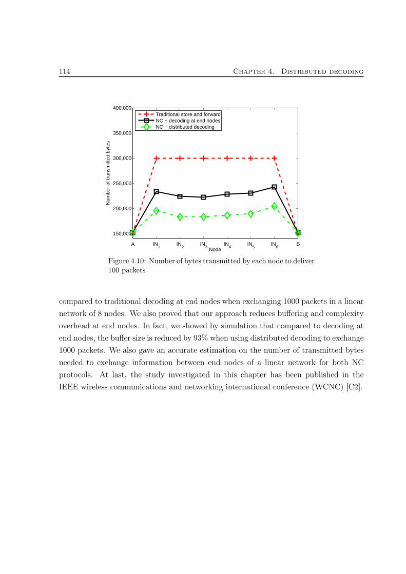
114 Chapter 4. Distributed decoding
150,000
200,000
250,000
300,000
350,000
400,000N
umbe
r of
tran
smitt
ed b
ytes
NodeA IN
1IN
2IN
3IN
4IN
5IN
6B
Traditional store and forwardNC − decoding at end nodesNC − distributed decoding
Figure 4.10: Number of bytes transmitted by each node to deliver100 packets
compared to traditional decoding at end nodes when exchanging 1000 packets in a linearnetwork of 8 nodes. We also proved that our approach reduces buffering and complexityoverhead at end nodes. In fact, we showed by simulation that compared to decoding atend nodes, the buffer size is reduced by 93% when using distributed decoding to exchange1000 packets. We also gave an accurate estimation on the number of transmitted bytesneeded to exchange information between end nodes of a linear network for both NCprotocols. At last, the study investigated in this chapter has been published in theIEEE wireless communications and networking international conference (WCNC) [C2].

CHAPTER
5 Impact of packet loss on theperformance of NC
Without NC, lost packets have no impact on the delivery of other transmitted pack-ets. With NC, the packet loss may affect the decoding of other transmitted packets thusaffects the entire process of communication between nodes.
Since the publication of [3], researchers have concentrated on the use of NC for opti-mizing throughput in multicast networks [3,11,56] and for improving network reliabilitythrough random linear coding [16,57]. However, only few published works have consid-ered packet loss and packet loss recovery in the analysis of NC performance [58,59].
In traditional communication protocols, reliability relies on retransmissions, and endto end reliability is ensured by the transport layer of the OSI layered communicationstack. Transport layer uses ARQ, an error-control in data transmission that uses ac-knowledgments to achieve reliable data transmission over an unreliable service. More-over, hop to hop reliability is ensured by PHY and MAC layers by the mean of HARQ,ARQ and forward error correction (FEC). In this chapter, ARQ refers to end to endARQ of the transport layer.
Recently, hop by hop transport layer reliability protocols have been developed whereintermediate nodes store and recover packets to deliver data more efficiently [60, 61].With NC, reliability and throughput gain are achieved through linear NC [4, 11] whereseveral packets are linearly combined together and broadcasted into the network. Severalpublished works in the literature have dealt with the benefits of NC from the reliabilitypoint of view [57,62].
In [57], authors have presented analytical and numerical results for the performance ofend-to-end and link-by-link reliability mechanisms based on ARQ, FEC and NC in a treetopology. Using an access point topology with k receivers, they have demonstrated thatthe reliability gain of NC compared to ARQ is in Θ(log k). They have also shown thatallowing intermediate nodes to recover lost packets remains in Θ(log k) while furtherminimizing the number of transmissions. However, it should be noted that bufferingpackets at intermediate nodes requires decoding coded messages which might be costly.
115

116 Chapter 5. Impact of packet loss on the performance of NC
In this chapter, models presented in Section 3.1 are used to perform generating, cod-ing, decoding and transmission activities on packets of the network. The impact of lostpackets on buffering and complexity at the receiving nodes is studied and two new mech-anisms are proposed to allow the recovery of the lost packets. Compared to traditionalrecovery protocols, our mechanisms provide a significant performance improvement interms of number of transmissions required to recover from packet loss.
Due to lossy nature of wireless channel conditions, recent works have focused on lossrecovery taking into consideration the overhead on the network due to retransmissions.In [63] authors have proposed codecast protocol suitable to low-loss, low-latency con-straint applications such as video streaming. Their work is based on random NC [11]implementing localized loss recovery and path diversity with very low overhead. Theydemonstrated throughout simulations that codecast achieves a near-perfect packet deliv-ery ratio while maintaining at the same time lower overhead than conventional multicast.They have concluded that routing and route selection have major impact on reliabilityand time delivery.
To reduce loss impact, routing selection mechanisms have been investigated. In[64] overlay routing networks have been proposed to monitor communication betweennodes in order to improve routing of packets and provide loss reduction over traditionalrouting algorithms. Opportunistic routing [65–67] dynamically selects paths based onloss conditions. However, in [68] authors conducted a comparison of best-path routingand opportunistic routing and found that the benefit of opportunistic routing is muchless than commonly believed. It should be well noted that these mechanisms introduceslatency on the overall communication time and overhead on the routing nodes. Themechanisms we are proposing are network independent and require no probe from thenetwork.
In the majority of cases, NC is considered as block coding where packets can only bedecoded in batches [69]; in this context, a coded message, needs to wait for the arrival ofother coded messages before being able to be decoded. While NC increases throughputand lowers congestion, block decoding may cause major delays and reduce QoS. Recentworks have focused on QoS and proposed methods to reduce the average waiting time inthe buffer of the intermediate nodes [54,70]. Our work differs from existing works in thesense that we use NC for data exchange activity and not for multicast purposes. Withour proposed ACNC protocol, no delay is engendered by the coding activity and no

5.1. Loss with centralized decoding 117
packet is delayed waiting for a match. Moreover, instantaneous decoding at end nodes isguaranteed when packets arrive in order. Decoding remains guaranteed in real networkswhere messages arrive unordered.
Our contributions in this chapter are summarized as follows:• For both decoding at end nodes and distributed decoding, the impact of packet loss
on the decoding capability at the receivers and the decoding perturbation causedby each loss are investigated and analyzed.• For decoding at end nodes, two new recovery mechanisms initiated by end nodes are
proposed to handle packet loss with NC; i) immediate retransmission request (IRR)mechanism that uses information extracted from the undecodable messages torequest the retransmission of lost packets. ii) recovery from packet loss mechanismwith a basic covering set discovery (BCSD) that allows near optimal number ofretransmissions to recover lost packets.• For distributed decoding, a loss detection and recovery mechanism (LDRM) is
presented. LDRM uses NC received messages as feedback for packet delivery andautomatically adds potentially lost packets to the list of arrivals that needs to betransmitted.
5.1 Loss with centralized decoding
In a linear network of 4 nodes, Figure 5.1 shows a detailed trace of packets exchangedbetween end nodes A and B where node A generates packets Pai i = 1, 2, ... and node B
generates packets Pbi i = 1, 2, ... . A maturity value µ = 3 is set for the network and eachpacket is upper-indexed by its age. Recall from Chapter 3 that solid arrows indicateunicast activity to the next hop while dashed arrows indicate broadcast activity of newlycoded messages. With the use of aging, redundant copies of packets quickly disappearfrom the network. For example, packet Pa1 generated at iteration 1 is removed from allmessages in the network at iteration 7.
In this context, we are mainly interested in the impact of losing a coded message,on the decoding capability at the receiving node. For example, if message (Pa1 ⊕ Pb2)between nodes IN2 and B at iteration 3 is lost, node B successively receives codedmessages that the node is unable to decode.
Figure 5.2 shows another trace conducted on a network with 5 nodes where the

118 Chapter 5. Impact of packet loss on the performance of NC
Figure 5.1: Delivery of packets in a network with no loss
Figure 5.2: Delivery of packets in a network with 5 nodes

5.1. Loss with centralized decoding 119
Figure 5.3: Losing one packet in a network with 5 nodes
life cycle of two packets Pa1 and Pb6 is observed. The network is synchronized andtransmissions occur only at the starting of each iteration. Note that in such case, theabsorbing effect conserves a maximum cardinality of 3 for any generated coded message.
In Figure 5.3, a packet loss occurs at iteration 7 between IN2 and IN3 creating adiscrepancy with Figure 5.2 that lasts till iteration 13. The perturbation caused by thepacket loss increases both the number of transmissions as seen at iterations 9 and 10and the cardinality of coded messages as seen at iteration 12.
5.1.1 Packet loss simulation
Algorithms presented in section 3.1 are used to run simulations on a linear network of6 nodes, i.e. with 4 intermediate nodes. Statistics are recorded about packet loss impacton the decoding opportunity and buffering time at end nodes. In this simulation, only thehop IN3 → IN2 is considered with loss and the packet loss is modeled as an independentand identical Bernoulli distributed process. The objectives of this simulation is twofold;first, understand the correlation between the packet loss and the number of undecodablepackets at the receiver. Second, aid to establish a recovery process to minimize thenumber of retransmissions.

120 Chapter 5. Impact of packet loss on the performance of NC
0 5% 10% 15% 20%0
2%
4%
6%
8%
10%
12%
14%
16%P
erce
ntag
e of
und
ecod
ed p
acke
ts
Loss probability P
Maturity 6Maturity 8Maturity 10
Figure 5.4: Percentage of undecodable packets with different lossprobabilities and different maturities
5.1.2 Correlation between lost and undecodable messages
The percentage of undecoded packets is presented in figure Figure 5.4 for 10000packets exchanged between nodes A and B is 10000 for different loss probabilities. Thepercentage of undecodable packets corresponds to the percentage of different packetsthat have been identified in the header of the received messages without being decoded.The simulation is repeated for 3 different maturity values. Figure 5.4 shows the impactof the aging concept on the number of undecodable messages. As shown in the figure,the number of undecodable packets at the receiving node increases with maturity. Thisis justified by the fact that when the maturity factor increases, coded packets live longerin the network and are further coded with other packets leading to an increase in thenumber of undecodable packets at the receiver. Moreover, the number of undecodablepackets at the receiver is finite and the system resumes receiving decodable packets aftereach loss.
In Figure 5.5 the buffering of received packets at destinations is studied. Destina-tion nodes need to buffer sent and received packets to be used in the decoding process.

5.1. Loss with centralized decoding 121
0 5% 10% 15% 20%0
5%
10%
15%
20%
25%
30%P
erce
ntag
e of
the
buffe
ring
time
Loss probability P
Average (Maturity 6)Highest (Maturity 6)Average (Maturity 8)Highest (Maturity 8)Average (Maturity 10)Highest (Maturity 10)
Figure 5.5: Buffering versus loss percentage
Buffering is costly since it requires significant memory space. Buffering time of a packetis computed as the laps of time between the moment the packet was received and the lasttime the packet was used for decoding other packets. The figure gives the percentage ofthe buffering time with respect to the total communication time versus the loss proba-bility P , for 3 different maturity values, i.e. 6, 8 and 10. Furthermore, for each case,the highest values and the average values are represented. These results show that thebuffering time decreases when the loss percentage increases. This is justified by the factthat less decoding occurs when more coded messages are lost. Moreover, the bufferingalso varies with maturity. When maturity increases, packets live longer in the networkand the required maximum buffering time increases thus more buffering is needed.
5.1.3 Decoding opportunity
In this section we study the multiplicity of the lost packets in the network and itsimpact on the decoding process. By multiplicity, we mean the number of copies ofthe packet that exist in the network. Recall that, when a packet is coded with otherpackets, the resulting message is broadcasted into the network creating duplicates of

122 Chapter 5. Impact of packet loss on the performance of NC
Figure 5.6: Lost packet discovery
these packets. When a packet is lost, other copies of that packet still exist in thenetwork creating messages that cannot be decoded at the receiver.
To clarify how end nodes can receive undecodable messages, consider the exampleshown in Figure 5.6. In this example, a coded message m is created and broadcasted atiteration l by node INj (shown in the figure as m1 and m2 which are identical). Considernow that message m1 is lost and m2 reaches node INi. All packets in m2 originatedfrom A are flagged as exist at destination ("Exist at dest." flag set to true). Node INi
uses message m2 in further coding activity and broadcasts at iteration l+1 a new codedmessage m
′ ⊕m2. Node B cannot decode m′ ⊕m2 since it holds more than one packet
originated by A and unknown to B.With a maturity µ, Theorem 3 presented in Chapter 3 sets a boundary on the
dissemination of each packet in the network. Note that, each packet can be found ina maximum of 2µ messages. Due to the linear nature of the network, each end nodereceives a maximum of 2µ
2messages containing the same packet. This upper bound on
the multiplicity of a packet is used in the following theorem to estimate the number ofundecodable messages when a packet is lost.
Theorem 6. Given a network G = (N,E) and a maturity scalar µ in N+. When apacket loss occurs in the direction of end node E, the estimated number of undecodablemessages that can be received by E as a result of that loss is given by
1
µ+ 1
µ∑i=2
2µ−i (5.1)
Proof. If a packet in the direction of E is lost at age 0, i.e. before being coded, no othercopies of that packet exist in the network. Consequently, no undecodable messages arereceived by E. On the other hand, if a packet is lost in the direction of E at maturity

5.1. Loss with centralized decoding 123
age, the other copy of that packet is unicasted in the opposite direction. Consequently,no undecodable messages are received by E. Let P a be a packet with age a, and NPa
be the number of messages received by E that are created starting from P a. Accordingto Theorem 6, NP
a = 2µ−a
2. Referring to the coding graph presented in Chapter 3, we
assume that in a network with maturity µ, there is an equal probability that a lostpacket has an age between 0 and µ. The total number of undecodable messages thatcan be received by E is:
1
µ+ 1
µ−1∑i=1
NPi =
1
µ+ 1
µ−1∑i=1
2µ−i
2=
1
µ+ 1
µ−1∑i=1
2µ−(i+1)
By taking i+ 1 = j, we can write
1
µ+ 1
µ∑j=2
2µ−j
�
As an example, a packet loss might lead to receiving 4 undecodable messages whenmaturity is set to 6, after which the system resumes receiving decodable messages.
Another important factor that helps reducing the number of received undecodablemessages is related to the model presented in Section 3.1. Recall that the model allowspackets to be transmitted without coding and never waits for a match. A simulationis performed to study the number of packets that are traveling through the networkwithout being coded. Figure 5.7 shows the number of uncoded messages in the outgoingqueue of each node of the network. End nodes generate packets while they receive thelowest percentage of undecodable messages. There is however, a significant percentageof uncoded packets floating between the nodes of the network. This is in fact due to thefollowing factors:• Aging: preventing packets from being further coded.• Decision model: forcing packets to be transmitted without waiting for a match.Analysis in this section shows an interesting characteristic of NC when it comes
to lossy network. The intensive use of NC, represented by a large maturity value,keeps duplicates of a lost packet in the network and the number of undecodable packetsincreases. One of the advantages of aging is that it helps creating mature messages inthe network thus preventing coupling with duplicates of lost packets.

124 Chapter 5. Impact of packet loss on the performance of NC
0
20%
40%
60%
80%
100%
120%
A IN1
IN2
IN3
IN4 B
Per
cent
age
of u
ncod
ed p
acke
ts in
the
queu
e
Node
Receiving queueSending queue
Figure 5.7: Percentage of uncoded messages at each node
5.2 Recovery from packet loss in centralized decoding
With NC, recovery from packet loss differs from traditional retransmission protocolssince packets are interconnected together by the mean of coded messages. We haveshown that losing one packet might lead to lose additional packets due to the nature ofthe coded messages and of the decoding process. For this reason, an efficient algorithmis needed in order to minimize the number of retransmissions.
To remedy from packet loss and its effect, two new mechanisms are detailed in thissection. To further evaluate the performance of these mechanisms, a revised version ofthe LNC protocol is also presented first.
5.2.1 Revised LNC protocol
The revised LNC protocol uses block coding as follows; each sending node groups b
packets together (Pi i = 1 to b) and sends b∆ linearly independent combinations of thepackets in each group. In this case the coding matrix M and the created combinations

5.2. Recovery from packet loss in centralized decoding 125
Yj j = 1 to ∆ are illustrated as follows:
M =
g11 g12 ............ g1b
g21 g22 ............ g2b
... ... ............ ...
g∆1 g∆2 ............ g∆b
with X =
P1
P2
...
...
Pb
and Y = MX
The cardinality b of each block and the number of combinations b∆ are determinedaccording to Theorem 6 and according to the loss percentage between the end nodes ofthe network given by:
Pn = 1− (1− P )N−1 (5.2)
where N is the total number of nodes and P is the probability of loss in a link.Once Pn is identified, the sending node needs to send b∆ =
⌈b
1−Pn
⌉independent linear
combinations of the packets of each block to guarantee the delivery of the packets in theblock. In order to minimize the number of transmissions, the cardinality of the blockshould be selected to satisfy b
1−Pn=⌈
b1−Pn
⌉.
Furthermore, each loss in the network leads according to Theorem 6, to have Un =1
µ+1
∑µi=2 2
µ−i undecodable messages that might reach the destination. With Pn as losspercentage in the network, Un × Pn undecodable messages can reach the end node. Tobypass the undecodability problem, b∆ is augmented by Pn × b∆ × Un × (1− Pn).
5.2.2 Immediate retransmission request
The end node receiving an undecodable message is able to identify, by reading theheader of the undecodable message, those packets having the "exist at dest." = true butare not in its buffered packets for decoding purpose. Without waiting for a retransmissionevent from the upper layer (i.e. transport layer) a retransmission request is initiated bythe NC protocol for these packets.
Due to delays and unordered arrival of messages at the receiver, one undecodablemessage is not a sign of packet loss. The receiving node suspects that a loss occurs whenundecodable messages remain undecodable for a specific period of time, denoted byttime (threshold on time) or when receiving a certain number of consecutive undecodable

126 Chapter 5. Impact of packet loss on the performance of NC
messages, denoted by tcup (threshold on consecutive undecodable packets).
Algorithm 10 Immediate Retransmission Request
1: cup=0, i=1, rr=false, rp = ∅2: while i ≤ number of UM do3: Add to rp the undelivered packets in UM(i)4: if UM(i) and UM(i-1) are consecutive then5: Increment cup6: if cup ≥ tcup then7: rr = true8: end if9: else
10: cup=011: end if12: if Current time - Receiving time of UM(i) ≥ ttime then13: rr = true14: end if15: Increment i16: end while17: if rr = true then18: Request all needed packets in rp19: end if
The Immediate Response Request (IRR) algorithm is designed to take into consider-ation the previously mentioned concerns. The IRR algorithm is shown in Algorithm 10where UM denotes an undecodable message. The algorithm works as follows: initially,consecutive undecodable packets (cup) is set to 0, request retransmission (rr) is set tofalse and the list of requested packets (lrp) is empty. The algorithm then iterates oneach entry in the list of undecodable messages. Lines 4 to 11 are dedicated to identifyconsecutive undecodable messages and a request for retransmission is initiated if cup
reaches a predefined threshold. Lines 12 to 14 investigate the buffering time of eachundecodable message and request retransmission if a threshold on time is reached. Therequests for packet retransmissions are sent in the header of newly generated packetsor immediately if no new packets are available for transmission. Since no buffering ofpackets is performed at the intermediate nodes, the requests for retransmission is sent tothe generator nodes. The algorithm is initiated each time the node is about to performa decoding activity.

5.2. Recovery from packet loss in centralized decoding 127
0 5% 10% 15% 20%0
2%
4%
6%
8%
10%P
erce
ntag
e of
req
uest
ed p
acke
ts
Loss probability P
Maturity 6Maturity 8Maturity 10
Figure 5.8: IRR: percentage of requested packets versus lossprobability
IRR differs from the end to end ARQ of the transport layer. IRR is faster to bothidentify lost packets and to initiate a retransmission request. However, it should benoted that IRR does not replace ARQ. As shown in the proof of Theorem 6, a packetmight be lost leaving no decoding consequences at the receiving nodes. Such lost canonly be detected and requested by the transport layer using ARQ.
The simulation results of IRR are shown in Figure 5.8. The simulation ran with the3 values of maturity and with the same conditions in Figure 5.4. Figure 5.8 shows thatthe number of requested packets increases with maturity values for the same packet losspercentage. Furthermore, the number of retransmissions compared to the number ofreceived undecodable messages is presented in Table 5.2 for two loss percentages, wherethe undecodable and the requested columns are extracted from the results of Figures5.4 and 5.8 respectively. Table 5.2 reveals a reduction in the percentage of requestedpackets when maturity increases. This is justified by the fact that, with larger maturity,a loss generates more undecodable messages and a retransmission helps also decodingmore packets.

128 Chapter 5. Impact of packet loss on the performance of NC
Table 5.1: Percentage of retransmission versus undecodable
Loss probability P10% 20%
Maturity undecodable Requested Percentage undecodable Requested Percentage6 280 205 73.2% 634 486 76.7%8 577 371 64.3% 954 615 64.5%10 798 503 63.0% 1381 865 62.6%
Table 5.2: Percentage of retransmission versus undecodable
5.2.3 Minimal retransmission request
Before presenting this new recovery process, we introduce some definitions and pro-pose a mechanism to identify the packets to be requested from the sender in order torecover all lost packets with minimal retransmissions.
Closures and covering sets
Let S be a set of packets and C be a set of coded messages.
Definition 20. When XOR operation is used to code packets together, the simple clo-sure of S, denoted by S+
C , is the set of packets that can be decoded from C using packetsin S.
To better understand the simple closure definition, we illustrate the following exam-ple.
Let S = {p1, p2, p3} and C = {p1p4, p1p3p5, p4p5p7, p5p6p7, p6p8p9, p7p8p9}To build the simple closure of S, we proceed as follows:
S+C = {p1, p2, p3}
S+C = {p1, p2, p3, p4} using p1p4
S+C = {p1, p2, p3, p4, p5} using p1p3p5
S+C = {p1, p2, p3, p4, p5, p7} using p4p5p7
S+C = {p1, p2, p3, p4, p5, p7, p6} using p5p6p7
Definition 21. When linear combination is used to code packets together, the complexclosure of S, denoted by S++
C , is the set of packets that can be decoded, by the mean ofGaussian Elimination, from C using packets in S.
Going back to the previous example, the complex closure of S, is denoted by:

5.2. Recovery from packet loss in centralized decoding 129
S++C = S+
C ∪ {p8, p9}
where p8 and p9 can be obtained by solving the system:{α1p8 + α2p9 = R1
β1p8 + β2p9 = R2
Where R1 and R2 are the received coded packets and (α1, α2)t and (β1, β2)
t are thecorresponding coding vectors normally included in the header of the received codedpackets.
Definition 22. S is a covering set of C if the closure of S includes all packets thatare part of the coded messages in C.
Going back again to the previous example, we see that S++C is a covering set of C
but S+C is not.
Definition 23. A basic covering set of C is a covering set of C with minimal cardi-nality (having the least number of packets).
Basic covering set discovery
The recovery process starts when end node receives a message that cannot be de-coded, i.e. it has more than one unknown packet. At that time, the end node expects toreceive additional undecodable packets. Each received undecodable message is XOR-edwith all known packets and the resulting chunk of undecodable packets XOR-ed togetheris added to an originally empty set C.
The gathering period of undecodable chunks of messages is controlled by a timerthat starts immediately after the reception of the first undecodable message. As statedbefore, undecodability might be caused by unordered arrival of messages and the problemmight be solved without intervention when more messages arrive to the end node. Theduration of the timer is an application specific parameter based on the communicationmedium and the type of application. It can vary from milliseconds in the case of instantmessaging where messages need to be delivered in order to the upper layer, to secondsin the case of file exchange where only the complete file needs to be ordered. When thetimer times out, the recovery mechanism is lunched. The recovery mechanism consistsof finding a basic covering set and packets in the covering set are requested from thesender. The Basic Covering Set Discovery (BCSD) algorithm is presented in Algorithm

130 Chapter 5. Impact of packet loss on the performance of NC
Algorithm 11 Basic covering set discovery (BCSD)1: Build the incident matrix M2: B an empty set3: repeat4: i = 15: maxj = 06: max1 = 07: for j = 1 to NbColumns do8: if sum of 1’s in column j > max1 then9: maxj = j
10: max1 = sum of 1’s in column j11: end if12: end for13: add maxj to B14: Remove column maxj15: repeat16: if there is a row with one entry then17: Remove the row and column of that entry18: end if19: until No more columns can be removed20: until Matrix is empty21: Request packets in B from the sender
11. The algorithm follows a greedy mechanism that tries, within a reasonable amountof time to identify a basic covering set for all chunks of messages in C. The algorithmstarts by building the incident matrix where columns identify the packets in C androws represent undecodable chunks of messages sorted by receiving time. For the setC = {p1p4, p1p3p5, p4p5p7, p5p6p7, p6p8p9, p7p8p9} the corresponding incident matrix M
is:
M =
p1 p3 p4 p5 p6 p7 p8 p9
p1p4 1 1
p1p3p5 1 1 1
p4p5p7 1 1 1
p5p6p7 1 1 1
p6p8p9 1 1 1
p7p8p9 1 1 1

5.2. Recovery from packet loss in centralized decoding 131
Figure 5.9: BCSD example
The algorithm then iterates on the incident matrix until the covering set is built. At eachiteration, the column with the highest number if 1’s is selected (i.e. highest occurrencein the undecodable messages) and the corresponding packet is added to the covering setB. If more than one row with the same highest number of 1’s are present, then anyone of these rows can be selected. Rows with one entry are then removed together withthe column of the entry since the corresponding packet can be decoded. The algorithmstops when the incident matrix becomes empty.
Steps applying BCSD algorithm to the incident matrix M are shown in Figure 5.9and the basic covering set found is {p5, p7, p8}. First the algorithm selects P5 to be inthe covering set since it corresponds to the column with the highest number of 1’s. Theassociated column is removed and the resulting matrix is shown in Figure 5.9b. Thesecond iteration of the algorithm selects P7. However, removing its associated columnleaves rows b and c with exactly one packet each so both columns b and c and rows b
and c are removed creating an additional decoding opportunity at rows d and e. Figure5.9c shows the resulting matrix at the end of iteration 2. Finally, packet P8 (or P9) isselected at iteration 3 to complete the covering set.
5.2.4 Simulation results
In this section, both IRR and BCSD algorithms are implemented and tested. Sim-ulations run on a linear network of 6 nodes when a loss probability is applied on eachlink. Results are compared to both traditional store and forward with ARQ protocolsand to the revised LNC protocol. Note that the revised LNC uses the same decisionmodels presented in Section 3.1. Along the simulations, 10000 packets are exchanged

132 Chapter 5. Impact of packet loss on the performance of NC
0 5% 10% 15% 20%35000
40000
45000
50000
55000
60000
65000
70000
75000
80000T
otal
num
ber
of tr
ansm
issi
ons
Loss probability P
Traditional store and forwardNC with IRRNC with BCSDLinear network coding
Figure 5.10: Total number of transmissions required to deliver10000 packets
between both end nodes of the network. Algorithms are compared according to the totalnumber of transmissions needed to deliver all the exchanged packets between the endnodes. In the SF protocol, the transport layer at the end nodes automatically claimsunacknowledged packets. The total number of transmissions to reliably deliver all thepackets is recorded. In a reliable network of 6 nodes, 5 transmissions are needed todeliver each packet from one end node to another. The performance of IRR and BCSDare also evaluated and compared to LNC and SF.
Results are presented in Figure 5.10. Traditional store and forward algorithm startswith a total of 50000 transmissions on a reliable network and ends with an increase of34% when the loss probability reaches 20%.
Moreover, on a reliable network, revised LNC, IRR and BCSD start with almostthe same number of required transmissions to deliver all the packets. When the lossprobability increases, the number of transmissions with the revised LNC increases about56% when the loss probability reaches 20%. Both IRR and BCSD show an importantsaving in the number of transmissions when compared to the revised LNC. With a lossprobability of 20%, BCSD presents a saving of 22% in the number of transmissions over

5.2. Recovery from packet loss in centralized decoding 133
0 5% 10% 15% 20%12
13
14
15
16
17
18
19
20
21
22
23
Tot
al ti
me
in s
econ
ds
Loss probability P
Revised LNCNC with IRRNC with BCSD
Figure 5.11: Total delivery time of the 10000 packets exchanged
the revised LNC. IRR slightly increases the number of transmissions compared to BCSD.Figures 5.11 and 5.12 show respectively the total delivery time and the average
delivery time for the three competing mechanisms. The total delivery time is computedas the time elapsed between the transmission of the first packet and the reception of thelast one while the delivery time of a packet is computed as the time between the firsttransmission of the packet and its delivery. In these simulations, each transmission fromone node to an adjacent one requires 1 millisecond of time. As shown in Figure 5.12,the revised LNC overcomes the proposed mechanisms when it comes to average deliverytime. This is justified by the fact that no retransmission is requested. With the revisedLNC, the slow increase in the average delivery time is due to the time needed at thereceiver to gather enough messages of each block in order to decode the packets of theblock. As for our proposed mechanisms, IRR bypasses BCSD when it comes to averagedelivery time, since IRR reacts immediately when a loss is detected while BCSD waitslonger to gather undecodable messages and reduce the size of the covering set, i.e. thenumber of retransmissions.

134 Chapter 5. Impact of packet loss on the performance of NC
0 5% 10% 15% 20%1150
1200
1250
1300
1350
1400
1450
1500
1550
Ave
rage
tim
e in
ms
Loss probability P
Revised LNCNC with IRRNC with BCSD
Figure 5.12: Average delivery time.
5.3 Loss with distributed decoding
In this section, a new coding mechanism is provided to automatically detect andrecover lost packets in wireless lossy networks that employs distributed decoding. Con-trary to the majority of ARQ algorithms relying on acknowledgment, our mechanismextracts feedback on packet delivery by analyzing received network coded messages andautomatically reacts when packet loss is sensed.
In WSN and WMN, channels are subject to interference, fading, noise and limitedbandwidth. ARQ is a conventional method for error recovery applied in a hop by hopmanner at the link layer of the OSI model or in an end-to-end manner at the transportlayer. ARQ requires the sender to be aware of the packet loss using negative acknowl-edgment (NACK) or timeout before requesting or initiating retransmission of the lostpacket. This process is time consuming and not suitable for real time communication.Fault-tolerant techniques in WSN and WMN initially focus on routing mechanisms toimprove reliability in an efficient way. We now propose a mechanism able to deal withloss in a distributed fashion.

5.3. Loss with distributed decoding 135
5.3.1 Reliable data transfer
With distributed decoding, intermediate nodes buffer packets to be used for decod-ing. Our novel loss recovery protocol is based on the idea of taking advantage of thisbuffering mechanism to retransmit packets when a loss is detected. With the proposedprotocol, the loss recovery process is decentralized and no acknowledgment or packetretransmission request is needed.
Definition 24. In networking, Promiscuous mode is a mode for a wired or wirelessnetwork interface controller that causes the controller to pass all traffic it receives to thecentral processing unit rather than passing only the frames that the controller is intendedto receive.
When node i transmits, to neighboring nodes, a message containing a new packetPr that is newly arrived to i, it expects to receive back exactly one coded message,for an example MPr containing packet Pr. If no coding opportunity is found for Pr
at a neighboring node, Pr is unicasted to its destination and node i, initially set inpromiscuous mode overhears the transmission of Pr. If Pr is not received or overheardin a message within a specific amount of time, node i initiates a loss recovery process byadding packet Pr to the receiving queue for a possible coding and transmission activity.
The proposed mechanism requires end nodes to acknowledge newly received packetsand hence distributed decoding protocol is modified to enable this acknowledgmentwithout additional transmissions. End nodes code with each new packet ready to betransmitted, all previously received packets since the last transmission. The resultingcoded message is unicasted to the next hop of the newly generated packet. If there existno packet to transmit, received packets from the same source since the last transmissionare coded and sent to that source.
There are two possible reasons for node i not to receive or overhear message MPr :
1. MPr was lost during its transmission to neighboring node.
2. MPr was lost when transmitted to node i.
Before going further with our loss detection and recovery mechanism (LDRM), somedefinitions are needed to clarify some of its aspects.
Definition 25. The round trip RTij(Pr) of a packet Pr between nodes i and j is de-fined as the time elapsed between the transmission of Pr as a single packet or within acoded message and the time Pr is received back from node j coded within a message oroverheard. Nodes i and j can be intermediate or end nodes.

136 Chapter 5. Impact of packet loss on the performance of NC
Proposition 1. Given a transmission rate R, a propagation speed S, the distance Dbetween nodes i and j, and a coded message length of L bits, the round trip RTij(Pr) isgiven by:
RTij(Pr) = 2×(L
R+
D
S
)+Btj (5.3)
where Btj is the average buffering time at node j.
Proof. By definition, the round trip of a packet equals to the sum of its transmissiontime from i
(LR
), its propagation time to j
(DS
)its buffering time at j and the trip
back. �Definition 26. The set i+ is defined as the set of all neighboring nodes to i.
Definition 27. The round trip RT+i (Pr) of a packet Pr between node i and all nodes
in i+ is defined as the time elapsed between the transmission of Pr as a single packet orwithin a coded message and the time Pr is received back or overheard from every nodein i+.
Proposition 2. The rount trip RT+i (Pr) is given by
RT+i (Pr) = max
jRTij(Pr) j ∈ i+ (5.4)
Algorithm 12 describes our LDRM and works as follows: when a message is receivedby node i from a neighboring node k, packets in the message are scanned and comparedto buffered packets in B (lines 1, 2 and 3). When a match is found, say for packet Pm,buffered packet Pm is removed from the message by XORing Pm it with the message.The header of the message is also updated (lines 4 and 5). As part of the loss detectionand recovery process, packet Pm in B is flagged as being received by node k. On theother hand, being already flagged as received by k is an indication that node k did notreceive from i a message containing Pm and a retransmission is required. In this case,the Pm is included in the next outgoing message to k as an acknowledgment (lines 6, 7, 8and 9). After removing all matching packets from the received message, the cardinalityof the message is checked. If the cardinality is set to 1, the remaining packet is new tonode i and it is added to the buffer B and its buffering timer starts as part of the lossdetection process (lines 14, 15 and 16). If a buffered packet times out in B and it is notflagged as received by all neighboring nodes, the packet is broadcasted to neighboringnodes and the timer of that packet is reset (lines 18, 19, 20 and 21).

5.3. Loss with distributed decoding 137
Algorithm 12 LDRM: when receiving packet from k
1: for each packet Pi in the received message do2: for each packet Pj in the buffer B do3: if Pi = Pj then4: message = message ⊕ Pj
5: Remove from the message the header of Pi
6: if Pj not flagged as received by k then7: flag Pj as received by k8: else9: include Pj in the list of packets to k
10: end if11: end if12: end for13: end for14: if cardinality of the message is 1 then15: add the single packet to B16: start buffering timer for the newly added packet17: end if18: if a packet in B times out then19: if Not received by all neighboring nodes then20: add the timed out packet to the outgoing queue21: reset the timer22: end if23: end if
5.3.2 Simulation results
The LDRM algorithm is validated by running simulations on linear network of 6nodes. Simulations are completed using a self-developed JAVA-based application thatsimulates the network layer at each node of the network and the transport layer atend nodes for traditional end-to-end ARQ technique. The packet loss is modeled as anindependent and identical Bernoulli distributed process on all links.
LDRM is compared with a modified version of the distributed decoding protocolpresented in Section 4.1 that uses end-to-end ARQ to recover from packet loss. Themodified version, named DNC-ARQ works as follows: an acknowledgment (ACK) is sentby end nodes for each received and decoded packet. ACKs are grouped and included inthe transmitted packets, or sent individually if no packet has to be transmitted.
Figure 5.13 shows the number of transmissions required to exchange 10000 packets

138 Chapter 5. Impact of packet loss on the performance of NC
0 5% 10% 15% 20%30000
31000
32000
33000
34000
35000
36000
37000
38000
39000
40000N
umbe
r of
req
uire
d tr
ansm
issi
ons
Loss probability P
LDRMDNC−ARQ
Figure 5.13: Total number of transmissions needed to deliver10000 packets
(5000 packets generated by each end node) between the two end nodes of the network.The simulation is run for different loss percentages and the number of transmissionsneeded is recorded for both LDRM and DNC-ARQ mechanisms. It can be observedthat the proposed scheme outperforms the traditional ARQ process in terms of numberof retransmissions when the loss probability on each link increases. For a network with20% loss probability, the number of saved transmissions with LDRM exceeds 35000. Thisis due to 1) ARQ is an end-to-end mechanism while LDRM is a hop-by-hop mechanism.Thus one packet loss with ARQ requires retransmitted packet to travel over 5 links whilea packet loss with LDRM requires a packet to travel only to next hop.
Figure 5.14 shows the time needed to deliver all 10000 packets for both algorithms.In these simulations, each transmission from one node to an adjacent one requires 1millisecond of time. The total delivery time is the time elapsed between the transmissionof the first packet and the reception of the last one. As it can be seen on Figure 5.14, bothalgorithms have similar performances though LDRM still slightly outperforms DNC-ARQ.
Figure 5.15 shows the average delivery time of a packet between end nodes. This

5.3. Loss with distributed decoding 139
0 5% 10% 15% 20%11
12
13
14
15
16
17
18
19
20
21
22T
otal
tim
e in
sec
onds
Loss probability P
LDRMDNC−ARQ
Figure 5.14: Total time needed to deliver 10000 packets
0 5% 10% 15% 20%36
38
40
42
44
46
48
50
52
54
56
58
60
Tot
al ti
me
in m
illis
econ
ds
Loss probability P
LDRMDNC−ARQ
Figure 5.15: Average time needed to reliably deliver a packetbetween end nodes

140 Chapter 5. Impact of packet loss on the performance of NC
is the time for a packet, in average, to travel from an end node to another. The weakperformance of DNC-ARQ is clear from this figure and justified by the fact that foreach loss, an end node needs at least 5 transmissions time to report a loss and another5 transmission times to receive lost packet. Moreover, the hop-by-hop loss detection isfrom far, faster than an end-to-end loss detection.
5.4 Conclusion
This chapter dealt with the impact of packet loss in NC, where the models presentedin Section 3.1 have been used to study packet loss effect on the decoding process at endnodes. Simulations have shown that with the proposed model and with the use of aging,any perturbation caused by losing packets is finite in time and end nodes receive a limitednumber of undecodable packets. The number of undecodable packets at end nodes hasbeen analytically and experimentally studied under the effect of aging and NC activitieswhere two new mechanisms have been proposed to improve NC performance in lossynetworks. The first mechanism, called IRR, immediately requests lost packets when apacket loss occurs and the second mechanism, called BCSD, requests missing packets ina reduced number of transmissions. Simulation results have shown that in typical cases,both algorithms help reducing by 22% the number of transmissions comparing to therevised LNC protocol. Finally it should be noted that IRR and the revised LNC aremore suitable to some applications like video conferencing where the average deliverytime is needed to be reduced while BCSD is more convenient to file exchange where thetotal delivery time needs to be optimized.
We have also studied in this chapter the loss problem with distributed decodingand proposed LDRM algorithm for loss recovery. Contrary to the majority of ARQmechanisms, LDRM uses NC received messages as feedback for packet delivery andautomatically adds potentially lost packets to the list of arrivals that needs to be trans-mitted. Simulation has shown that LDRM not only reduces the number of requiredtransmissions comparing to traditional end-to-end ARQ but also improves the deliverytime of packets thus enhancing the QoS. At last, the impact of loss with distributed de-coding investigated in this chapter has been accepted in 23rd international conference onSoftware, Telecommunications and Computer Networks (SoftCOM 2015) [ C1] while theimpact of loss with decoding at end nodes has been part of the journal paper submitted

5.4. Conclusion 141
to EURASIP [A1].


Conclusion and Perspectives
Conclusion
In this thesis, we have proposed a new network coding protocol based on addresscorrelation (ACNC) of packets exchanged between end nodes. This protocol is based ontwo decoding methods, the centralized decoding taking place at the end nodes and thedistributed decoding where all intermediate nodes participate in the decoding process.We have started this thesis with a general overview on the NC theory, focusing mainly onthe advantages of this technology. It is well noted that the continuous increase on band-width demand makes such technology a requirement for future communication. Then,we have listed the wide application areas of NC, which can be divided into bandwidthsaving and reliability .
Since this thesis focuses on both bandwidth saving and reliability, we have introducedin Chapter 2, the ACNC protocol as the starting point of our studies. ACNC is acomplete NC based protocol that guarantees a certain level of QoS and 100% decodabilityat the receiving nodes. Both centralized and distributed decoding are based on ACNC.
In the next part of the thesis, namely in Chapter 3, we have presented the cen-tralized decoding protocol where decoding occurs at the receiving nodes only. Withthis approach, intermediate nodes are only responsible for coding and forwarding codedmessages to destinations. This approach is studied from different perspectives:
First, we have presented two decision models to mange intermediate and end nodeactivities respectively. For intermediate nodes, the decision model is deterministic andtries to balance the occupation of the receiving and the outgoing queues. By doing so,the risk of packet drop due to receiving queue being full is reduced. For end nodes, aprobabilistic model is used that better simulates the packet generation and delivery to
143

144 Conclusion
the upper layer of the OSI model.Second, we have analyzed the cardinality of the coded messages in the network and
demonstrate the possibility of infinite growth in the cardinality, thus in the size of thecoded messages. To rectify, we have proposed a solution based on the aging conceptwhere each packet is given an age. Packets get older in time with each participation intoa coding activity. When reaching maturity, packets are no more allowed to participateto be coded together. This process limits the life cycle of the packets and helps reducingthe cardinality of the coded messages in the network.
Buffering requirements at end nodes for decoding purposes and decoding complexityare also studied for the centralized decoding approach. We have shown that the bufferingsize and the complexity are proportional to the number of packets exchanged during theestablished connection between end nodes. We have also demonstrated that the conceptof aging reduces buffering requirements at end nodes.
After studying the centralized decoding, we have developed in Chapter 4 the dis-tributed decoding which reduces the buffering and the complexity at end nodes bydistributing these resource requirements over the nodes of the network. Thus withdistributed decoding, buffering is required at intermediate nodes also but the overallbuffering size is dramatically reduced. The basic idea behind distributed decoding isto involve the intermediate nodes of the network to engage in the decoding process byremoving redundancies of delivered packets from the coded messages thus reducing theircardinality.
We have studied in Chapter 5 the loss impact and the loss recovery for both cen-tralized and distributed decoding. We have proposed solutions for fast recovery andreliably deliver all packets exchanged in lossy networks. These solutions are based onsome learning mechanism that anticipates loss detection and rapidly initiates a recoveryprocess. The advantages of these solutions is that sending nodes are not involved in therecovery process and no acknowledgment is needed to identify lost packets.
As a conclusion, this thesis has presented a contribution for the enhancement ofthe NC protocols by defining a novel approach for coding, routing and reliably deliverpackets in wireless linear networks while taking into account some constraints as QoSand resource requirements. The new proposed protocols can be considered as modelsfor bandwidth management in the next generation of wireless communication systems.

Conclusion 145
Perspectives
Many interesting areas and prospects can be further investigated for future worksbased on this thesis:
First, the work carried out in this thesis has proven the efficiency of ACNC to enhancethroughput and reliability in wireless linear networks. Further comparison with otherNC protocols can be performed either to identify its superiority or detect and enhanceweaknesses. Models presented in Chapter 3 can be generalized to support other possiblenode activities. Furthermore, the study methods applied and shown in Figures 3.4,3.12, 4.2 and 5.3 to identify coding activities and the impact of network changes can beapplied in further networking studies. The coding graph used for counting the number oftransmissions an the coding opportunities can be carried out for more complex networktopologies.
Second, the efficiency of ACNC in wireless linear networks can be extended to randomwired and wireless networks. In this case, coding opportunities can be enhanced beyondaddress correlation as we did in RCNC. An example of such enhancement can be seenin multicast communication networks, where more than 2 end nodes are exchanginginformation. Coding at intermediate nodes can be conducted only on packets involvedin a multicast session.
Third, security can be carried out as an enhancement to ACNC where coding nodesneed to authenticate the originated nodes of potential address correlated packets forcoding. Secured ACNC can be of benefit for cloud computing where data integrityand security are some of the major concerns when it comes to cloud computing andvisualization.
Fourth, the proposed ACNC can be carried out with real implementation in variousexisting and emerged paradigms as AdHoc, WSN, the Internet of things (IoT), 5G andHeterogeneous Networks (HetNet). WSN and the IoT that utilize low-cost informationgathering and dissemination can benefits from NC to save on throughput and energyconsumption. ACNC can be used as an efficient mean of communication between sensors.To this purpose, a token that travels between pairs of nodes can be used for bothgathering and dissemination.
Finally, cross layer ACNC can be carried out as throughput enhancement along theOSI layers of communication systems. Since NC can be implemented at any of the OSI

146 Conclusion
layers, an additive network coding approach where NC is applied on more than one layeris an interesting research avenue.

Bibliography
[1] S. Sankaranarayanan, P. Papadimitratos, A. Mishra, and S. Hershey, “A bandwidth sharing ap-proach to improve licensed spectrum utilization,” in First IEEE International Symposium on NewFrontiers in Dynamic Spectrum Access Networks, 2005. DySPAN 2005. IEEE, 2005, pp. 279–288.
[2] S. Katti, S. Gollakota, and D. Katabi, “Embracing wireless interference: Analog network coding,”in ACM SIGCOMM Computer Communication Review, vol. 37, no. 4. ACM, 2007, pp. 397–408.
[3] R. Ahlswede, N. Cai, S.-Y. R. Li, and R. W. Yeung, “Network information flow,” IEEE Transactionson Information Theory, vol. 46, no. 4, pp. 1204–1216, 2000.
[4] S.-Y. R. Li, R. W. Yeung, and N. Cai, “Linear network coding,” IEEE Transactions on InformationTheory, vol. 49, no. 2, pp. 371–381, 2003.
[5] R. Koetter and M. Médard, “An algebraic approach to network coding,” IEEE/ACM Transactionson Networking (TON), vol. 11, no. 5, pp. 782–795, 2003.
[6] C. Gkantsidis and P. R. Rodriguez, “Network coding for large scale content distribution,” in INFO-COM 2005. 24th Annual Joint Conference of the IEEE Computer and Communications Societies.Proceedings IEEE, vol. 4. IEEE, 2005, pp. 2235–2245.
[7] S. Katti, H. Rahul, W. Hu, D. Katabi, M. Médard, and J. Crowcroft, “Xors in the air: practicalwireless network coding,” IEEE/ACM Transactions on Networking (ToN), vol. 16, no. 3, pp. 497–510, 2008.
[8] Z. Shengli, S.-C. Liew, and P. P. Lam, “Physical layer network coding,” arXiv preprintarXiv:0704.2475, 2007.
[9] F. Xue, C.-H. Liu, and S. Sandhu, “Mac-layer and phy-layer network coding for two-way relay-ing: Achievable regions and opportunistic scheduling,” in Proceedings of the 45th Annual AllertonConference on Communication, Control and Computing, vol. 128. Citeseer, 2007.
[10] S. Jaggi, P. Sanders, P. Chou, M. Effros, S. Egner, K. Jain, L. M. Tolhuizen et al., “Polynomial timealgorithms for multicast network code construction,” IEEE Transactions on Information Theory,vol. 51, no. 6, pp. 1973–1982, 2005.
[11] T. Ho, M. Médard, R. Koetter, D. R. Karger, M. Effros, J. Shi, and B. Leong, “A random linearnetwork coding approach to multicast,” IEEE Transactions on Information Theory, vol. 52, no. 10,pp. 4413–4430, 2006.
[12] C. Fragouli, J.-Y. Le Boudec, and J. Widmer, “Network coding: an instant primer,” ACM SIG-COMM Computer Communication Review, vol. 36, no. 1, pp. 63–68, 2006.
147

148 Conclusion
[13] M. Langberg, A. Sprintson, and J. Bruck, “The encoding complexity of network coding,”IEEE/ACM Transactions on Networking (TON), vol. 14, no. SI, pp. 2386–2397, 2006.
[14] R. K. Ahuja, T. L. Magnanti, and J. B. Orlin, “Network flows,” DTIC Document, Tech. Rep.,1988.
[15] T. Wang and G. B. Giannakis, “Complex field network coding for multiuser cooperative com-munications,” IEEE Journal on Selected Areas in Communications,, vol. 26, no. 3, pp. 561–571,2008.
[16] T. Ho, R. Koetter, M. Medard, D. R. Karger, and M. Effros, “The benefits of coding over routingin a randomized setting,” in Proc. 2003 International Symposium on Information Theory, 2003.
[17] J. Irvine and D. Harle, Data communications and networks: An engineering approach. John Wiley& Sons, 2002.
[18] J. L. Van Wyk, A. Helberg, and L. Grobler, “Comparing the implementation of network coding ondifferent osi layers,” North West University, Potchefstroom Campus, 2009.
[19] J. Jannotti, D. K. Gifford, K. L. Johnson, M. F. Kaashoek et al., “Overcast: reliable multicastingwith on overlay network,” in Proceedings of the 4th conference on Symposium on Operating SystemDesign & Implementation-Volume 4. USENIX Association, 2000, pp. 14–14.
[20] Y. Zhu, B. Li, and J. Guo, “Multicast with network coding in application-layer overlay networks,”Selected Areas in Communications, IEEE Journal on, vol. 22, no. 1, pp. 107–120, 2004.
[21] D. Koutsonikolas, C.-C. Wang, and Y. C. Hu, “Efficient network-coding-based opportunistic routingthrough cumulative coded acknowledgments,” vol. 19, no. 5. IEEE Press, 2011, pp. 1368–1381.
[22] J. K. Sundararajan, D. Shah, M. Médard, S. Jakubczak, M. Mitzenmacher, and J. O. Barros,“Network coding meets tcp: Theory and implementation,” Proceedings of the IEEE, vol. 99, no. 3,pp. 490–512, 2011.
[23] C. Robinson and P. Kumar, “Sending the most recent observation is not optimal in networkedcontrol: Linear temporal coding and towards the design of a control specific transport protocol,”in Decision and Control, 2007 46th IEEE Conference on. IEEE, 2007, pp. 334–339.
[24] S. Ahmed and S. S. Kanhere, “Vanetcode: network coding to enhance cooperative downloadingin vehicular ad-hoc networks,” in Proceedings of the 2006 international conference on Wirelesscommunications and mobile computing. ACM, 2006, pp. 527–532.
[25] L. Scalia, F. Soldo, and M. Gerla, “Piggycode: a mac layer network coding scheme to improvetcp performance over wireless networks,” in IEEE Global Telecommunications Conference, 2007.GLOBECOM’07. IEEE, 2007, pp. 3672–3677.
[26] S. Zhang, S. C. Liew, and P. P. Lam, “Hot topic: physical-layer network coding,” in Proceedings ofthe 12th annual international conference on Mobile computing and networking. ACM, 2006, pp.358–365.
[27] H. Rahul, H. Hassanieh, and D. Katabi, “Sourcesync: a distributed wireless architecture for ex-ploiting sender diversity,” ACM SIGCOMM Computer Communication Review, vol. 41, no. 4, pp.171–182, 2011.

Conclusion 149
[28] S. C. Liew, S. Zhang, and L. Lu, “Physical-layer network coding: Tutorial, survey, and beyond,”Physical Communication, vol. 6, pp. 4–42, 2013.
[29] L. Chen, T. Ho, M. Chiang, S. H. Low, and J. C. Doyle, “Congestion control for multicast flowswith network coding,” IEEE Transactions on Information Theory,, vol. 58, no. 9, pp. 5908–5921,2012.
[30] Y. E. Sagduyu and A. Ephremides, “Cross-layer optimization of mac and network coding in wirelessqueueing tandem networks,” IEEE Transactions on Information Theory,, vol. 54, no. 2, pp. 554–571, 2008.
[31] K.-H. Lee and J.-H. Kim, “Cross-layer design for tcp splitting connections with network coding indvb-rcs networks,” in 2014 International Conference on Information and Communication Technol-ogy Convergence (ICTC),. IEEE, 2014, pp. 970–973.
[32] K. Narayanan, M. P. Wilson, and A. Sprintson, “Joint physical layer coding and network cod-ing for bi-directional relaying,” in Proc. of Allerton Conference on Communication, Control andComputing, 2007.
[33] H. Seferoglu, A. Markopoulou, and K. Ramakrishnan, “I 2 nc: intra-and inter-session networkcoding for unicast flows in wireless networks,” in INFOCOM, 2011 Proceedings IEEE. IEEE,2011, pp. 1035–1043.
[34] D. S. Lun, M. Médard, and R. Koetter, “Network coding for efficient wireless unicast,” in 2006International Zurich Seminar on Communications. IEEE, 2006, pp. 74–77.
[35] D. S. Lun, M. MéDard, R. Koetter, and M. Effros, “On coding for reliable communication overpacket networks,” Physical Communication, vol. 1, no. 1, pp. 3–20, 2008.
[36] M. Ghaderi, D. Towsley, and J. Kurose, “Network coding performance for reliable multicast,” inMilitary Communications Conference, 2007. MILCOM 2007. IEEE, 2007, pp. 1–7.
[37] A. G. Dimakis, P. Godfrey, Y. Wu, M. J. Wainwright, and K. Ramchandran, “Network codingfor distributed storage systems,” IEEE Transactions on Information Theory, vol. 56, no. 9, pp.4539–4551, 2010.
[38] J. Widmer and J.-Y. Le Boudec, “Network coding for efficient communication in extreme networks,”in Proceedings of the 2005 ACM SIGCOMM workshop on Delay-tolerant networking. ACM, 2005,pp. 284–291.
[39] D. Wang, Q. Zhang, and J. Liu, “Partial network coding: Theory and application for continuoussensor data collection,” in IWQoS 2006. 14th IEEE International Workshop on Quality of Service,2006. IEEE, 2006, pp. 93–101.
[40] K. Bhattad and K. R. Narayanan, “Weakly secure network coding,” NetCod, Apr, vol. 104, 2005.
[41] N. Cai and R. W. Yeung, “Secure network coding,” in 2002 IEEE International Symposium onInformation Theory, 2002. Proceedings. IEEE, 2002, p. 323.
[42] ——, “Secure network coding on a wiretap network,” IEEE Transactions on Information Theory,vol. 57, no. 1, pp. 424–435, 2011.

150 Conclusion
[43] Z. Yu, Y. Wei, B. Ramkumar, and Y. Guan, “An efficient signature-based scheme for securingnetwork coding against pollution attacks,” in INFOCOM 2008. The 27th Conference on ComputerCommunications. IEEE. IEEE, 2008.
[44] S. Jaggi, M. Langberg, S. Katti, T. Ho, D. Katabi, and M. Médard, “Resilient network coding inthe presence of byzantine adversaries,” in INFOCOM 2007. 26th IEEE International Conferenceon Computer Communications. IEEE. IEEE, 2007, pp. 616–624.
[45] H. Guo, Y. Qian, K. Lu, and N. Moayeri, “The benefits of network coding over a wireless backbone,”in Global Telecommunications Conference, 2009. GLOBECOM 2009. IEEE. IEEE, 2009, pp. 1–6.
[46] L. Mitten, “Branch-and-bound methods: General formulation and properties,” Operations Re-search, vol. 18, no. 1, pp. 24–34, 1970.
[47] E. Balas, S. Schmieta, and C. Wallace, “Pivot and shifta mixed integer programming heuristic,”Discrete Optimization, vol. 1, no. 1, pp. 3–12, 2004.
[48] J. Eckstein, “Parallel branch-and-bound algorithms for general mixed integer programming on thecm-5,” SIAM Journal on Optimization, vol. 4, no. 4, pp. 794–814, 1994.
[49] C. Fragouli, D. Lun, M. Médard, and P. Pakzad, “On feedback for network coding,” in InformationSciences and Systems, 2007. CISS’07. 41st Annual Conference on. IEEE, 2007, pp. 248–252.
[50] T. Ohira and R. Sawatari, “Phase transition in a computer network traffic model,” Physical ReviewE, vol. 58, no. 1, p. 193, 1998.
[51] D. Nguyen, T. Tran, T. Nguyen, and B. Bose, “Wireless broadcast using network coding,” IEEETransactions on Vehicular Technology, vol. 58, no. 2, pp. 914–925, 2009.
[52] R. Kumar, S. Tati, F. De Mello, S. V. Krishnamurthy, and T. L. Porta, “Network coding aware rateselection in multi-rate ieee 802.11,” in Network Protocols (ICNP), 2010 18th IEEE InternationalConference on. IEEE, 2010, pp. 92–102.
[53] B. Haeupler, M. Kim, and M. Médard, “Optimality of network coding with buffers,” IEEE Infor-mation Theory Workshop (ITW), pp. 533–537, 2011.
[54] W. Chen, K. B. Letaief, and Z. Cao, “Buffer-aware network coding for wireless networks,”IEEE/ACM Transactions on Networking, vol. 20, no. 5, pp. 1389–1401, 2012.
[55] C. Ibars, L. Giupponi, and S. Addepalli, “Distributed multiple access and flow control for wirelessnetwork coding,” IEEE 71st Vehicular Technology Conference (VTC 2010-Spring), pp. 1–6, 2010.
[56] A. Agarwal and M. Charikar, “On the advantage of network coding for improving network through-put,” in Information Theory Workshop, 2004. IEEE, 2004, pp. 247–249.
[57] M. Ghaderi, D. Towsley, and J. Kurose, “Reliability gain of network coding in lossy wireless net-works,” in IEEE INFOCOM 2008. The 27th Conference on Computer Communications. IEEE,2008.
[58] S. Rayanchu, S. Sen, J. Wu, S. Banerjee, and S. Sengupta, “Loss-aware network coding for unicastwireless sessions: design, implementation, and performance evaluation,” in ACM SIGMETRICSPerformance Evaluation Review, vol. 36, no. 1. ACM, 2008, pp. 85–96.

Conclusion 151
[59] D. S. Papailiopoulos, J. Luo, A. G. Dimakis, C. Huang, and J. Li, “Simple regenerating codes:Network coding for cloud storage,” in 2012 IEEE Proceedings INFOCOM. IEEE, 2012, pp. 2801–2805.
[60] J. F. Mingorance-Puga, G. Maciá-Fernández, A. Grilo, and N. M. C. Tiglao, “Efficient multime-dia transmission in wireless sensor networks,” in 6th EURO-NF Conference on Next GenerationInternet (NGI). IEEE, 2010, pp. 1–8.
[61] H. Lee, Y. Ko, and D. Lee, “A hop-by-hop reliability support scheme for wireless sensor networks,”in Fourth Annual IEEE International Conference on Pervasive Computing and CommunicationsWorkshops. PerCom Workshops. IEEE, 2006, pp. 5–pp.
[62] C. Fragouli, D. Katabi, A. Markopoulou, M. Medard, and H. Rahul, “Wireless network coding: Op-portunities & challenges,” in MILCOM 2007. IEEE Military Communications Conference. IEEE,2007, pp. 1–8.
[63] J.-S. Park, M. Gerla, D. S. Lun, Y. Yi, and M. Medard, “Codecast: a network-coding-based adhoc multicast protocol,” IEEE Wireless Communications, vol. 13, no. 5, pp. 76–81, 2006.
[64] D. G. Andersen, A. C. Snoeren, and H. Balakrishnan, “Best-path vs. multi-path overlay routing,”Proceedings of the 3rd ACM SIGCOMM conference on Internet measurement, pp. 91–100, October2003.
[65] S. Biswas and R. Morris, “Opportunistic routing in multi-hop wireless networks,” ACM SIGCOMMComputer Communication Review, vol. 34, no. 1, pp. 69–74, 2004.
[66] K. Zeng, W. Lou, and H. Zhai, “Capacity of opportunistic routing in multi-rate and multi-hopwireless networks,” Wireless Communications, IEEE Transactions on, vol. 7, no. 12, pp. 5118–5128, 2008.
[67] S. Chachulski, M. Jennings, S. Katti, and D. Katabi, “Trading structure for randomness in wirelessopportunistic routing,” vol. 37, no. 4, 2007.
[68] Z. Zhong and S. Nelakuditi, “On the efficacy of opportunistic routing,” 4th Annual IEEE Commu-nications Society Conference on Sensor, Mesh and Ad Hoc Communications and Networks, 2007.SECON’07., pp. 441–450, June 2007.
[69] W.-L. Yeow, A. T. Hoang, and C.-K. Tham, “Minimizing delay for multicast-streaming in wirelessnetworks with network coding,” in INFOCOM 2009, IEEE. IEEE, 2009, pp. 190–198.
[70] E. Drinea, L. Keller, and C. Fragouli, “Real-time delay with network coding and feedback,” PhysicalCommunication, vol. 6, pp. 100–113, 2013.


Institut National des Sciences Appliquées de Rennes20, Avenue des Buttes de Coëmes CS 70839 F-35708 Rennes Cedex 7Tel : 02 23 23 82 00 - Fax : 02 23 23 83 96
N° d’ordre : 15ISAR 19 / D15 - 19
Résumé
Le codage réseau (CR) est une nouvelle technique dans laquelle les données sont codées et décodées par les nœuds afin d’améliorer le débit et réduire les retards. En utilisant des algorithmes algébriques, le codage consiste à combiner les transmissions ensemble et le décodage consiste à restaurer ces transmissions. Cette opération réduit le nombre total de transmissions nécessaire pour échanger les données, mais requière plus de traitement au niveau des nœuds. NC peut être appliquée à l’une des couches ISO. Toutefois dans ce travail, l’accent est mis surtout au niveau de la couche réseau.
Dans ce travail, nous présentons des nouveautés de CR pour construire des protocoles afin d’améliorer l’utilisation de la bande passante, la qualité de service et réduire l’impact de la perte de paquets dans les réseaux à pertes. Plusieurs défis ont été soulevés par cette thèse concernant les détails de codage et de décodage et tous les mécanismes connexes utilisés pour livrer les paquets échangés entre les nœuds. Notamment, des questions comme le cycle de vie des paquets dans le réseau, la cardinalité des messages codés, le nombre total d’octets transmis et la durée du temps de maintien des paquets ont été inspectés, analytiquement comptés, soutenus par de nombreux théorèmes puis vérifiés par des simulations. Dans les réseaux à pertes, les méthodes utilisées pour étudier de près le comportement du réseau conduisaient à la proposition de nouveaux mécanismes pour surmonter cette perte et réduire la surcharge.
Dans la première partie de la thèse, un aperçu du CR est mené depuis son déclanchement par Alshwede et al. Les différentes techniques sont détaillées mettant l’accent sur les codages linéaire et binaire. Ces techniques sont élaborées avec des exemples extraits de différents scénarios pour aider à comprendre les avantages et les inconvénients de chacune d’elles.
Dans la deuxième partie, un nouveau protocole basé sur la corrélation des adresses (ACNC) est présenté, et deux approches utilisant ce protocole sont introduites; l’approche centralisée où le décodage se fait aux nœuds d’extrémités et l’approche distribuée où chaque nœud dans le réseau participe au décodage. Le décodage centralisé est élaboré en présentant d’abord ses modèles de décision et le détail du décodage aux nœuds d’extrémités. La cardinalité des messages codés reçus et les exigences de mise en mémoire tampon au niveau des nœuds d’extrémités sont étudiées et les notions d’âge et de maturité ont été introduites. La méthode de décodage distribué est présentée comme une solution pour réduire la charge sur les nœuds d’extrémités en distribuant le processus de décodage et les exigences en mémoire tampon aux nœuds intermédiaires.
La Perte et le recouvrement en CR sont examinés pour les deux approches proposées. Pour l’approche centralisée, deux mécanismes pour limiter l’impact de la perte sont présentés. A cet effet, le concept de fermetures et des ensembles couvrant sont introduits et la découverte des revêtements optimaux afin de trouver l’ensemble optimal de paquets à retransmettre afin de décoder tous les paquets reçus est proposée. Pour le décodage distribué, un nouveau mécanisme de fiabilité hop-à-hop est proposé tirant profit du CR et permettant de se récupérer de la perte sans la nécessité
Abstract
Network coding (NC) is a new technique in which transmitted data is encoded and decoded by the nodes of the network in order to enhance throughput and reduce delays. Using algebraic algorithms, encoding at nodes accumulates various transmissions in fewer ones and decoding restores these transmissions. NC requires fewer transmissions to transmit all the data but more processing at the nodes. NC can be applied at any of the ISO layers. However, the focus is mainly on the network layer level.
In this work, we introduce novelties to the NC paradigm with the intent of building easy to implement NC protocols in order to improve bandwidth usage, enhance QoS and reduce the impact of losing packets in lossy networks. Several challenges were raised by this thesis concerning details in the coding and decoding processes and all the related mechanisms used to deliver packets between end nodes. Notably, questions like the life cycle of packets in coding environment, cardinality of coded messages, number of byte overhead transmissions and buffering time duration were inspected, analytically counted, supported by many theorems and then verified through simulations. When the packet loss problem was addressed, methods used in this thesis to closely investigate the behavior of the network as a response to the loss led to the proposition of novel mechanisms to overcome this loss and to help reducing the overhead caused by packet loss.
In the first part of the thesis, an overview of NC is conducted since triggered by the work of Alshwede et al. NC techniques are then detailed with the focus on linear and binary NC. These techniques are elaborated and embellished with examples extracted from different scenarios to further help understanding the advantages and disadvantages of each of these techniques.
In the second part, a new address correlated NC (ACNC) protocol is presented and two approaches using ACNC protocol are introduced, the centralized approach where decoding is conducted at end nodes only and the distributed decoding approach where each node in the network participates in the decoding process. Centralized decoding is elaborated by first presenting its decision models and the detailed decoding at end nodes procedure. Moreover, the cardinality of received coded messages and the buffering requirements at end nodes are investigated and the concepts of aging and maturity were introduced. The distributed decoding approach is presented as a solution to reduce the overhead on end nodes by distributing the decoding process and buffering requirements to intermediate nodes.
Loss and recovery in NC are examined for both centralized and distributed approaches. For the centralized decoding approach, two mechanisms to limit the impact of loss are presented. To this effect, the concept of closures and covering sets are introduced and the covering set discovery is conducted on undecodable messages to find the optimized set of packets to request from the sender in order to decode all received packets. For the distributed decoding, a new hop-to-hop reliability mechanism is proposed that takes advantage of the NC itself and depicts loss without the need of an acknowledgement mechanism.
Copyright © 2022 FDOKUMEN