Centralized Cooperative Control for Route Surveillance With ...

Centralized Cooperative Control

For Route Surveillance

With Constant Communication

THESIS

Joseph D. Rosal, Capt, USAF

AFIT/GE/ENG/09-38

DEPARTMENT OF THE AIR FORCEAIR UNIVERSITY

AIR FORCE INSTITUTE OF TECHNOLOGY

Wright-Patterson Air Force Base, Ohio

APPROVED FOR PUBLIC RELEASE; DISTRIBUTION UNLIMITED.

The views expressed in this thesis are those of the author and do not reflect theofficial policy or position of the United States Air Force, Department of Defense, orthe United States Government.

AFIT/GE/ENG/09-38




THESIS

Presented to the Faculty

Department of Electrical and Computer Engineering

Graduate School of Engineering and Management

Air Force Institute of Technology

Air University

Air Education and Training Command

In Partial Fulfillment of the Requirements for the

Degree of Master of Science in Electrical Engineering

Joseph D. Rosal, B.S.E.E.

Capt, USAF

March 2009

APPROVED FOR PUBLIC RELEASE; DISTRIBUTION UNLIMITED.

AFIT/GE/ENG/09-38

CENTRALIZED COOPERATIVE CONTROL

FOR ROUTE SURVEILLANCE

WITH CONSTANT COMMUNICATION

Joseph D. Rosal, B.S.E.E.

Capt, USAF

Approved:

LtOlli;Jry J. Toussaint, PhD(Chairman)

date

Dr. Meir Pachter (Member) date

Dr. Richard Cobb (Member) date

AFIT/GE/ENG/09-38

Abstract

The route surveillance mission is a new application of unmanned aircraft sys-

tems (UASs) to meet the reconnaissance and surveillance requirements of combatant

commanders. The new mission intends to field a UAS consisting of unmanned aerial

vehicles (UAVs) that can provide day and night surveillance of convoy routes. This

research focuses on developing a solution strategy for the mission based on the ap-

plication of optimal control and cooperative control theory. The route surveillance

controller uses the UAS team size to divide the route into individual sectors for each

entity. A specifically designed cost function and path constraints are used to formu-

late an optimal control problem that minimizes the revisit time to the route and the

overall control energy of the UAS. The problem complexity makes an analytical so-

lution difficult, so a numerical technique based on the Gauss pseudospectral method

is used to solve for the optimal solution. The output trajectories describe a path

that each entity could fly to provide surveillance on the route. Simulated and real-

world routes containing likely urban and rural characteristics were used to test the

controller and show that the developed system provides feasible surveillance solutions

under certain conditions. These results represent baseline statistics for future studies

in this research area.

iv

Acknowledgements

I would like to thank my thesis advisor and committee for their unrelenting support

and guidance through this thesis effort. Ultimately, I could not have accomplished

this challenge without the love and support of my wife, parents, and brothers.

Joseph D. Rosal

v

Table of ContentsPage

Abstract . . . . . . . . . . . . . . . . . . . . . . . . . . . . . . . . . . . . . iv

Acknowledgements . . . . . . . . . . . . . . . . . . . . . . . . . . . . . . . v

Table of Contents . . . . . . . . . . . . . . . . . . . . . . . . . . . . . . . . vi

List of Figures . . . . . . . . . . . . . . . . . . . . . . . . . . . . . . . . . ix

List of Tables . . . . . . . . . . . . . . . . . . . . . . . . . . . . . . . . . . xii

List of Abbreviations . . . . . . . . . . . . . . . . . . . . . . . . . . . . . . xiii

I. Introduction . . . . . . . . . . . . . . . . . . . . . . . . . . . . . 11.1 Motivation . . . . . . . . . . . . . . . . . . . . . . . . . 11.2 Route Surveillance Mission . . . . . . . . . . . . . . . . 21.3 Problem Statement . . . . . . . . . . . . . . . . . . . . . 31.4 Thesis Organization . . . . . . . . . . . . . . . . . . . . 4

II. Background and Current Research . . . . . . . . . . . . . . . . . 6

2.1 Introduction . . . . . . . . . . . . . . . . . . . . . . . . . 62.2 Cooperative Control . . . . . . . . . . . . . . . . . . . . 6

2.2.1 Coupling . . . . . . . . . . . . . . . . . . . . . . 7

2.2.2 Cooperative search . . . . . . . . . . . . . . . . 9

2.3 Gauss Pseudospectral Method . . . . . . . . . . . . . . . 11

2.3.1 General Continuous-time Bolza Problem . . . . 132.3.2 GPM Discretization . . . . . . . . . . . . . . . . 14

2.4 Summary . . . . . . . . . . . . . . . . . . . . . . . . . . 17

III. Methodology . . . . . . . . . . . . . . . . . . . . . . . . . . . . . 19

3.1 Introduction . . . . . . . . . . . . . . . . . . . . . . . . . 193.2 Route Surveillance Controller . . . . . . . . . . . . . . . 193.3 Input Block . . . . . . . . . . . . . . . . . . . . . . . . . 21

3.3.1 Simulated routes . . . . . . . . . . . . . . . . . 213.3.2 Real-world routes . . . . . . . . . . . . . . . . . 22

3.4 K-means Algorithm Block . . . . . . . . . . . . . . . . . 22

3.5 Vehicle Dynamics Block . . . . . . . . . . . . . . . . . . 26

3.5.1 TACMAV model . . . . . . . . . . . . . . . . . 263.5.2 Communications Constraint . . . . . . . . . . . 283.5.3 Distance-from-route Constraint . . . . . . . . . 29

vi

6 Cost Function Block . . . . . . . . . . . . . . . . . . . . 323.6.1 Last-visit Time Concept . . . . . . . . . . . . . 33

3.6.2 Revisit Cost Function . . . . . . . . . . . . . . . 353.6.3 Control Energy Cost Function . . . . . . . . . . 40

3.7 Problem Setup Block . . . . . . . . . . . . . . . . . . . . 41

3.7.1 State, Control, and Path constraint limits . . . 42

3.7.2 Initial guess . . . . . . . . . . . . . . . . . . . . 44

3.7.3 PSCOL optimization . . . . . . . . . . . . . . . 44

3.8 Summary . . . . . . . . . . . . . . . . . . . . . . . . . . 45

IV. Analysis and Results . . . . . . . . . . . . . . . . . . . . . . . . 47

4.1 Introduction . . . . . . . . . . . . . . . . . . . . . . . . . 474.2 Performance Metrics . . . . . . . . . . . . . . . . . . . . 474.3 RS-UAS Controller Test Plan . . . . . . . . . . . . . . . 494.4 RS-UAS Controller Results . . . . . . . . . . . . . . . . 51

4.4.1 Route Surveillance Coverage . . . . . . . . . . . 51

4.4.2 Revisit Time . . . . . . . . . . . . . . . . . . . 604.4.3 Communications Constraint . . . . . . . . . . . 63

4.5 Summary . . . . . . . . . . . . . . . . . . . . . . . . . . 64

V. Conclusions and Recommendations . . . . . . . . . . . . . . . . . 655.1 Conclusions . . . . . . . . . . . . . . . . . . . . . . . . . 655.2 Future Research . . . . . . . . . . . . . . . . . . . . . . 67

Appendix A. Dimensionless UAV model . . . . . . . . . . . . . . . . . 70

Appendix B. Camera Field-of-View Approximation . . . . . . . . . . 74

Appendix C. K-means Clustering Algorithm . . . . . . . . . . . . . . 77

Appendix D. Dudek’s Taxonomy . . . . . . . . . . . . . . . . . . . . . 78

Appendix E. Additional Results . . . . . . . . . . . . . . . . . . . . . 81

E.1 Clicked Route 1 . . . . . . . . . . . . . . . . . . . . . . . 81E.2 Clicked Route 2 . . . . . . . . . . . . . . . . . . . . . . . 83E.3 Random Route 1 . . . . . . . . . . . . . . . . . . . . . . 87E.4 Texas Route 1 . . . . . . . . . . . . . . . . . . . . . . . 90E.5 Texas Route 2 . . . . . . . . . . . . . . . . . . . . . . . 94E.6 Clicked Route 3 . . . . . . . . . . . . . . . . . . . . . . . 97

vii

Page

Appendix F. Simulation Software . . . . . . . . . . . . . . . . . . . . 102

F.1 UAV generalMAIN . . . . . . . . . . . . . . . . . . . . . 102

F.2 UAV generalCost . . . . . . . . . . . . . . . . . . . . . . 103

F.3 UAV generaldae . . . . . . . . . . . . . . . . . . . . . . 104

F.4 UAV generalConnect . . . . . . . . . . . . . . . . . . . . 104

F.5 RSconstants and getConfiguration . . . . . . . . . . . . 104

F.6 Create route . . . . . . . . . . . . . . . . . . . . . . . . 105

Appendix G. PSCOL and TOMLAB Setup . . . . . . . . . . . . . . . 106

Bibliography . . . . . . . . . . . . . . . . . . . . . . . . . . . . . . . . . . 108

Vita . . . . . . . . . . . . . . . . . . . . . . . . . . . . . . . . . . . . . . . 111

viii

List of FiguresFigure Page

2.1. Example of perimeter surveillance configuration . . . . . . . . . 10

3.1. RS-UAS controller diagram . . . . . . . . . . . . . . . . . . . . 20

3.2. Random data set with K-means clustering applied . . . . . . . 24

3.3. Sample Texas road divided into four sectors . . . . . . . . . . . 25

3.4. Simulated UAVs banked at different angles . . . . . . . . . . . 28

3.5. UAV parallel to a section of road . . . . . . . . . . . . . . . . . 30

3.6. UAV offset from a route . . . . . . . . . . . . . . . . . . . . . . 32

3.7. FOV overlap mapped to one-dimensional road for first pass . . 33

3.8. FOV overlap mapped to one-dimensional road for return pass . 34

3.9. Sample augmented UAV history along a route. . . . . . . . . . 36

3.10. Sample FOV overlap on a route . . . . . . . . . . . . . . . . . 38

3.11. Sample last-visit time waveform . . . . . . . . . . . . . . . . . 39

3.12. Sample last-visit time waveform propagated in time . . . . . . 39

3.13. Example state limits for four sectors . . . . . . . . . . . . . . . 42

3.14. Example turn limits for two sectors . . . . . . . . . . . . . . . 43

3.15. Example initial guess for two sectors . . . . . . . . . . . . . . . 44

4.1. Example last-visit time function from a simulation . . . . . . . 48

4.2. Clicked route for Simulation 1 . . . . . . . . . . . . . . . . . . 50

4.3. Clicked route for Simulation 2 . . . . . . . . . . . . . . . . . . 50

4.4. Texas road last-visit time function for Phase 1 . . . . . . . . . 53



4.7. Legendre polynomial used by PSCOL . . . . . . . . . . . . . . 55

4.8. Sector 2 trajectory for Simulation 2 . . . . . . . . . . . . . . . 56

4.9. Simulation 4 initial guess and trajectories for Phase 1 and 3 . . 57

ix

Figure Page

4.10. Simulation 4 initial guess and trajectories for Phase 1 and 3 . . 58

4.11. Last-visit time function for Phase 1 and 3 of Simulation 5 . . . 59

4.12. Simulation 3 route and resulting sector trajectory . . . . . . . . 60

4.13. Simulation 6 control energy minimization . . . . . . . . . . . . 62

4.14. Communications spacing between UAV 1 and 2 . . . . . . . . . 64

B.1. Camera Field-of-view illustration . . . . . . . . . . . . . . . . . 74

B.2. Camera Field-of-view corner illustration . . . . . . . . . . . . . 75

E.1. Clicked route from Dayton for two UAVs . . . . . . . . . . . . 81

E.2. Sector trajectories over clicked Dayton road . . . . . . . . . . . 81

E.3. Clicked Road 1 last-visit time function for Phase 1 . . . . . . . 82



E.6. Clicked route from Dayton for four UAVs . . . . . . . . . . . . 84

E.7. Sector trajectories over clicked road for four UAVs . . . . . . . 85




E.11. Random road divided into three sectors . . . . . . . . . . . . . 88

E.12. Sector trajectories over random road for three UAVs . . . . . . 88

E.13. Random road last-visit time function for Phase 1 . . . . . . . . 89



E.16. Texas road divided into four sectors . . . . . . . . . . . . . . . 91

E.17. Sector trajectories over Texas road . . . . . . . . . . . . . . . . 92

E.18. Texas road last-visit time function for Phase 1 . . . . . . . . . 93



E.21. Partial Texas road divided into two sectors . . . . . . . . . . . 95

x

Figure Page

E.22. Sector trajectories over Simulation 2 . . . . . . . . . . . . . . . 95




E.26. Clicked Route 3 divided into three sectors . . . . . . . . . . . . 98

E.27. Sector trajectories over Clicked Route 3 . . . . . . . . . . . . . 99

E.28. Clicked Route 3 last-visit time function for Phase 1 . . . . . . . 100



xi

List of TablesTable Page

3.1. Sector lengths corresponding to Figure 3.3 . . . . . . . . . . . . 25

3.2. System specifications for the TACMAV . . . . . . . . . . . . . 27

3.3. Revisit-Cost variable definition . . . . . . . . . . . . . . . . . . 35

3.4. Path constraint limits . . . . . . . . . . . . . . . . . . . . . . . 43

4.1. RS-UAS controller test plan . . . . . . . . . . . . . . . . . . . . 49

4.2. Surveillance coverage over the route per phase . . . . . . . . . 52

4.3. Results from using smaller ∆max . . . . . . . . . . . . . . . . . 59

4.4. Surveillance coverage for Simulation 3 . . . . . . . . . . . . . . 60

4.5. Simulation travel-time ranges for each phase . . . . . . . . . . 61

4.6. Simulation revisit times for each phase . . . . . . . . . . . . . . 62

D.1. Dudek’s Taxonomy . . . . . . . . . . . . . . . . . . . . . . . . 80

E.1. Surveillance coverage for Clicked Route 1 . . . . . . . . . . . . 83


E.3. Surveillance coverage for random route . . . . . . . . . . . . . . 90

E.4. Surveillance coverage for Texas route . . . . . . . . . . . . . . . 94

E.5. Surveillance coverage for partial Texas route . . . . . . . . . . 97


F.1. Important simulation software files . . . . . . . . . . . . . . . . 102

xii

List of AbbreviationsAbbreviation Page

AFIT Air Force Institute of Technology . . . . . . . . . . . . . . 3

ANT Advanced Navigation Technology . . . . . . . . . . . . . . 4

CC cooperative control . . . . . . . . . . . . . . . . . . . . . . 7

DoD Department of Defense . . . . . . . . . . . . . . . . . . . . 1

FOV field of view . . . . . . . . . . . . . . . . . . . . . . . . . . 2

GPM Gauss pseudospectral method . . . . . . . . . . . . . . . . 15

GPS Global Positioning System . . . . . . . . . . . . . . . . . . 3

IEDs improvised explosive device . . . . . . . . . . . . . . . . . 1

KKT Karush-Kuhn-Tucker . . . . . . . . . . . . . . . . . . . . . 15

LG Legendre-Gauss . . . . . . . . . . . . . . . . . . . . . . . . 17

NLP nonlinear programming problem . . . . . . . . . . . . . . . 15

PSCOL Gauss pseudospectral optimization program . . . . . . . . 15

RS route surveillance . . . . . . . . . . . . . . . . . . . . . . . 3

RSCC Route Surveillance Cooperative Control . . . . . . . . . . 5

RS-UAS Route Surveillance-UAS . . . . . . . . . . . . . . . . . . . 3

TACMAV Tactical Micro Air Vehicle . . . . . . . . . . . . . . . . . . 4

UASs unmanned aircraft systems . . . . . . . . . . . . . . . . . 1

UAVs unmanned aerial vehicles . . . . . . . . . . . . . . . . . . . 2

3-DOF 3-degree of freedom . . . . . . . . . . . . . . . . . . . . . . 14

xiii




I. Introduction

1.1 Motivation

The Department of Defense (DoD) has taken increased interest in the employ-

ment of unmanned aircraft systems (UASs) as evidenced by published documents

outlining official concept of operations and promoting a department-wide roadmap

for future unmanned systems [1, 2]. With benefits such as reducing risk to human

life, performing dull, dirty, and dangerous missions, and an unwavering ability to fly

sorties without rest, UASs will continue to positively impact current conflicts. Dur-

ing Operations Enduring Freedom and Iraqi Freedom, UASs logged nearly 400,000

flight hours from October 2006 to October 2007 [2]. This statistic is still more im-

pressive with the inclusion of flight hours logged from other operations, and will only

increase with future advanced systems fulfilling the requirements established by the

“Unmanned Systems Roadmap 2007-2032” [2].

Combatant commanders have identified reconnaissance and surveillance as a

principal mission for UASs. Unmanned systems are well suited for this mission since

they are an effective tool to help acquire, process, and decipher information that is

relevant for today’s warfighter. Research that expands the capabilities of existing

UASs could have an immediate impact for current operations.

Improvised explosive devices (IEDs) continue to threaten current operations

and are one factor increasing the demand for unmanned systems. Emerging from the

need to protect coalition forces, a new concept of a surveillance mission was created to

mitigate the IED threat before a device is planted. The new mission attempts to stop

and counter the planting of IEDs on roadways by allowing a specifically designed UAS

1

to surveil routes commonly traveled by coalition forces. The primary objective of this

research is to apply optimal control theory and cooperative control theory to allow a

UAS to provide persistent surveillance of a roadway. The mission specifications will

be discussed in Section 1.2. Section 1.3 provides a problem statement for this research

along with assumptions based on the route surveillance mission.

1.2 Route Surveillance Mission

A representative route surveillance mission would be to field a UAS consisting

of four unmanned aerial vehicles (UAVs) that can provide day and night surveillance

of convoy routes. The system can be controlled from a single ground control unit.

The UAS should surveil areas of interest up to 60 miles in length with at least hourly

updates to every point along the route. There are two objectives of the proposed

UAS that are required for the route surveillance mission. The first is to minimize the

re-visit time over the route to better detect the planting of IEDs. The second is to

maximize the flight time of the system without losing surveillance of the route.

A requirement of the control algorithm is to automatically adjust coverage routes

when UAVs are retasked or need to be refueled. A communication system will provide

full bandwidth at a maximum distance of 20 miles. This constraint dictates that the

UAVs must reconfigure to maintain full bandwidth to communicate with other vehicles

and the ground station at the origin of the route.

The UAS must create a pattern such that each vehicle maintains surveillance

of the route and the ability to communicate with other vehicles. Each UAV preserves

surveillance by projecting its camera field of view (FOV), defined as the total viewing

window of the sensor, on the route at all times. Since the purpose of the surveillance is

to detect suspicious activity, the UAVs must stay within a certain distance and height

from the route to ensure each camera FOV provides constant imaging of the road.

Having identified the relevant aspects of the surveillance mission, the next section will

translate these overall objectives into a specific problem statement for this research

effort.

2

1.3 Problem Statement

Given the background information and the mission scenario, an overall problem

statement can be formulated as follows: apply optimal control theory to develop UAV

trajectories that efficiently meet the objectives of the route surveillance mission. The

collective system will be referred to as the route surveillance-UAS (RS-UAS) and must

provide constant surveillance on the route in order to achieve the mission objectives.

The RS-UAS controller divides each route into sectors and determines appropriate

trajectories for the UAS by applying an optimal control technique. The controller

is demonstrated by processing simulated and real-world routes to determine if the

trajectories provide constant surveillance and if the revisit time is minimized. Since

performance is determined through simulations, the routes and UAVs used in the

simulations must satisfy a variety of assumptions based on the RS mission and Air

Force Institute of Technology (AFIT) resources.

The first assumption is that the routes to be monitored will be well defined

for the simulation environment. This research assumes a well-defined route will have

a waypoint every quarter of a mile centered on the roadway and that the roadway

travels in a straight line between any two waypoints. Although terrain will not be

considered, the path shapes of urban and rural routes do differ greatly. The waypoint-

defined routes modeled with urban and rural characteristics will be simulated and

imported from a global positioning system (GPS) device.

The next assumption is that the UAVs will be treated as point masses controlled

by a capable autopilot. The number of UAVs will be capped at four aircraft per team

for two reasons. First, the route surveillance mission is intended to primarily operate

with team sizes of four aircraft. Second, the amount of processing time required to

optimize flight paths for larger team sizes using the current solution technique would

be impractical.

The third assumption is that the Tactical Micro Air Vehicle (TACMAV), owned

by the Advanced Navigation Technology (ANT) Center, flight characteristics have

3

been chosen to represent the UAVs modeled in this research. The operational RS-

UAS could be implemented as a man-portable weapon system, which is the intended

use of the TACMAV platform. Since the TACMAV’s camera resolution is much less

than the intended sensor for the RS mission, mission altitudes in this research will be

decreased to simulate a necessary pixel resolution. Adjusting for the actual camera

resolution and UAV can be easily accommodated in the RS-UAS controller.

The tailored mission considered by this research will have the following global

attributes:

• The candidate paths will be two-dimensional roads less than 60 miles in length.

• Terrain is assumed to be negligible at flight altitude.

• UAV communication bandwidth is assumed valid at distances less than 20 miles.

• The UAV altitude of 300 feet maintains appropriate pixel resolution.

• Wind will not be a contributing factor in the environment, so it is assumed to

be zero.

This research effort is a new investigation into the RS mission, so performance

metrics, such as the surveillance coverage and revisit time to the route, cannot be

compared to baseline statistics. Instead, the results of the investigation will establish

values for the performance metrics that could serve as an initial baseline for future

studies. The results show that the overall approach provides a satisfactory solution

to the RS problem under certain conditions.

1.4 Thesis Organization

Chapter II will provide key background concepts concerning cooperative con-

trol and optimal control problems. The route surveillance mission is categorized as a

cooperative search mission and compared to current research for trends in the control

architecture. As a result of studying current research with cooperative search mis-

4

sions, a numerical optimization technique is selected as the solution strategy for this

problem.

The RS-UAS controller is developed in Chapter III. The system architecture is

introduced and leads to the discussion of the K-means route division and the optimal

control problem solved by the numerical optimization software.

Chapter IV will define the metrics used to assess the performance of the con-

troller and present the test schedule developed for the RS-UAS controller. A set of

candidate routes that captured likely road shapes were used to demonstrate that the

controller can process routes with real-world characteristics. In addition, Chapter IV

provides an analysis and discussion of the results.

This research is concluded in Chapter V by offering closing remarks and sug-

gesting methods for expanding upon this research. Recommendations for future work

propose methods for improving the RS-UAS controller and taking this research be-

yond the assumptions outlined in Section 1.3.

5

II. Background and Current Research

2.1 Introduction

Since the route surveillance problem is a new area of research, this chapter

presents cooperative control (CC) search problems to determine a general solution

method that can be applied in the RS-UAS controller. As a result, an optimization

technique is selected to solve the route surveillance problem. Cooperative control and

its complex characteristics are defined in Section 2.2, which continues with an exami-

nation of current CC search problems. Section 2.3 discusses the Gauss pseudospectral

method and provides reasons for choosing a numerical method to solve the optimal

control problem. Section 2.4 summarizes the topics in this chapter used to develop

the basis for the methods implemented in the RS-UAS controller.

2.2 Cooperative Control

Cooperative control entails designing algorithms to control interactions between

entities in a cooperative system. “A cooperative system is defined to be multiple

dynamic entities that share information or tasks to accomplish a common, though

perhaps not singular, objective” [30]. An example of a cooperative system is a team

of UAVs performing a surveillance mission to gain knowledge of an area of operation.

The cooperative controller is the mechanism that controls the entities in this example.

An important function of an entity within a cooperative system is the capability to

communicate with others by actively passing information or passively observing other

entities [30]. Communication also plays a large role in identifying the properties and

solutions of CC problems.

Cooperative control systems have two general types of control structures: cen-

tralized and decentralized. In a centralized approach, a control algorithm is designed

to compute a solution assuming it has complete system knowledge. Because all of

the system information is available in one central location, this control structure pro-

duces optimal solutions for the system. The appropriate solution is transferred to

each entity resulting in cooperation.

6

Conversely, decentralized approaches distribute a copy of the control algorithm

throughout the entities in the system. Those embedded control algorithms compute

solutions based on necessary information received from other team members. This

approach is much harder to design because the embedded controllers cannot make

decisions assuming complete system knowledge, making the solutions suboptimal.

Unless a consensus building scheme is used to ensure identical information throughout

the embedded controllers, the overall cooperation will be limited [6].

Regardless of the control structure, the system achieves cooperation through

different methods and conditions of communication. In the centralized case, a form of

communication is required between the cooperative controller and the entities for this

structure to function. Alternatively, the decentralized structure requires communica-

tion between the entities so each embedded controller can function. In most cases,

the communication in the system is affected by its environment, which has different

impacts on the reliability and robustness of the two structures.

Any cooperative control problem poses its own challenges because of the many

driving forces within the system and its environment. Due to this complex nature,

designing a general approach for solving CC problems does not exist in the literature.

However, Beard, McLain, Chandler, Decker, and Martinez [6, 12, 14, 15, 28, 29] have

worked to classify and categorize cooperative search problems. Beard et al. [6] cate-

gorized the level of coupling between entity tasks and decisions to help an engineer

distill all of the system information down to an essential set required for cooperation.

Realizing the amount of coupling in this research effort, which is discussed in the next

section, will justify the control structure and methods presented in Chapter III.

2.2.1 Coupling. Defining varying levels of coupling between entities and

their tasks provides a method for gaining insight into a CC problem [6]. The four

categories that describe the level and type are objective, local, full, and dynamic

coupling. This CC characterization is important because the amount of coupling is

related to the achievable level of cooperation [6]. If a high degree of coupling exists in a

7

CC problem, then finding an approach for a valuable solution will be more demanding.

If that same CC problem can be translated in a manner which decreases coupling,

the solution method that achieves cooperation will be easier to find.

Objective coupling is the simplest and least restrictive incidence of coupling.

This situation can be defined when the decisions, costs, and outcomes of an entity do

not affect those of the other group members. In essence, the entities have influence on

their team members only through the constraint or objective that defines cooperation

and not through the direct impact on another entity.

The subsequent level of coupling is local coupling, which shares an attribute

with objective coupling. Each entity once again can influence team members through

the constraint or objective that defines cooperation. The key difference lies in the

fact that local coupling assumes the individual’s combined cost to the mission is a

function of its decisions and of its local neighbors’ decisions.

Full coupling represents the highest level of complexity where each entity affects

the decisions, costs, and outcomes of itself along with the entire group of collaborating

entities. In order for a single entity to decide to act, it must have knowledge of the

intentions of every other member on the team. The controller approach required for

this level of coupling will be highly complex.

The final category of coupling is dynamic coupling. This type is not defined

in terms of coupling in constraints or objectives defining cooperation but in terms

of coupling between shared physical cooperation. Consider a group of aircraft flying

in close formation attempting to benefit from the shared aerodynamics. Local cou-

pling exists between lead and follower aircraft because of the aerodynamic properties

affecting the follower and channeling back to the leader. The dynamic coupling in

this example is the physical interactions existing between each pair of aircraft in the

formation. Because of the physical implications, this category is typically treated in

a different manner than CC problems involving the other types of coupling.

8

Combining this technique of analyzing CC problems in conjunction with Dudek’s

taxonomy in Appendix D can provide a powerful advantage in identifying the crucial

elements of a CC problem. Determining the level of coupling will help an engineer

focus the control efforts on the elements that facilitate cooperation. In other words,

those critical characteristics affect the significance of the controlling mechanism. Now

that cooperative control has been introduced and a method to identify key elements

of CC problems has been discussed, current research in cooperative search missions

will be presented and used to select general methods to solve the route surveillance

problem.

2.2.2 Cooperative search. Since Decker’s summary of research regarding

cooperative search missions, the research focus has shifted from centralized approaches

with probabilistic methods [8,9,18,35] to distributed approaches where computation

and decision exist at the entity level [4, 6, 13, 19, 24, 25, 28, 29]. Chandler [12] found

that the current research using distributed algorithms can undertake increased levels

of coupling between local and global neighbors, while making the task of designing

useful systems much harder. Three works from current research, all implementing

distributed algorithms, have been selected to develop the foundation for the methods

implemented in Chapter III.

The work conducted by Kingston et al. [25] on perimeter surveillance with a

UAS is the most relevant research for the route surveillance problem. The authors

based their solution approach on the principles and perimeter surveillance problem

developed by McLain and Beard [6,29]. Essentially, the general perimeter surveillance

problem is reduced to a linear perimeter surveillance problem. Kingston et al. placed

the UAVs in a chain along the perimeter as illustrated in Figure 2.1. The UAVs are

assumed to communicate at the ends of their respective sectors where the coordina-

tion variable (the sector endpoints for each UAV) chosen by Kingston et al. can be

communicated. Coordination variables defined by McLain and Beard [6,29] represent

the minimum information required for each entity to decide how to achieve coopera-

9

Figure 2.1: Example of perimeter surveillance configuration used by Kingston etal. [25].

tion. The heuristic control law developed by Kingston et al. causes any two neighbors

that rendezvous to communicate essential information and then escort the neighbor

to the appropriate sector endpoint. Afterwards, the UAVs continue searching their

respective sectors. The authors showed that this control law eventually caused the

team of UAVs to settle into a balanced surveillance configuration (each UAV trav-

eled a portion of the evenly-divided route) on the perimeter even if some UAVs were

spontaneously removed from the system.

The distributed control law developed by Kingston et al. differs from the in-

tended control structure for this research, but the results are applicable. The authors

above showed that splitting the route into N sectors (where N is the number of ve-

hicles) produced a steady-state configuration for the UAS to provide surveillance in

the perimeter problem. This result will be used in the RS-UAS controller except that

communication with the other vehicles and ground control must be preserved while

each vehicle travels its sector. However, the type of surveillance in the research above

differs from that required in the route surveillance problem. The control algorithm

in this research, modeled after the centralized control structure, can provide optimal

surveillance trajectories.

The research efforts by McLain and Beard [6, 29] and Martinez et al. [28] aid

in selecting a solution approach for the RS-UAS controller. Those authors seek to

define cooperation constraints (McLain and Beard) or aggregate objective functions

(Martinez et al.) to distill the CC problem into a set of essential information for

the collective to obtain for cooperation. The method in which those functions are

10

produced comes from two distinct fields: one from simply studying and modeling

the CC problem under consideration and the other from systems theory or graph-

based knowledge. However, both sets of authors have come to the same general

structure for distributed algorithms: 1) define a function that captures cooperation,

2) optimize the function that in turn dictates the actions of each entity, and 3) ensure

that the collective group comes to a consensus on the essential information. The

current research effort is concerned with centralized control algorithms, but the first

two steps above will be applied to the RS-UAS controller developed in Chapter III. A

function must be created that captures the cooperative surveillance of the collective

team. Next, a method is required to optimize the orbit trajectories over the route.

The entities do not exchange cooperative information, but the communication between

entities must be maintained in order to collectively provide surveillance on the route.

The function created to capture cooperation in this research takes the form of a

cost function within an optimal control problem. The next section will describe how

a numerical optimization technique is required to overcome problem complexities.

2.3 Gauss Pseudospectral Method

Engineers have taken advantage of optimal control techniques in efforts to find

the best method to guide and control aerospace systems. There are two general

methods for solving optimal control problems. The first uses conditions for optimal-

ity to analytically solve for the optimal control. This approach is feasible for dynamic

systems with limited states, controls, and constraints. The second approach uses nu-

merical methods to solve for the optimal control. Although the problems are typically

transcribed to some sort of computer language, the classic conditions of optimality

are preserved.

In this research, numerical methods were chosen because the potential number

of states and controls makes an analytical solution impractical. Each first-order model

of the TACMAV includes five states and two control variables. If four UAVs are used

to provide surveillance of a route, analytically solving for optimality conditions be-

11

comes difficult with 20 states and 8 control variables. A 3-degree of freedom (3-DOF)

model like the one used by Kim [24] includes seven states and three control variables.

In this case, a four-UAV system would include 28 states and 12 control variables.

Model complexity only increases with a 6-DOF model. For those reasons, numerical

techniques are the preferred solution method, but there are additional design choices

required to solve the optimal control problem in this research.

Two general categories for solving continuous-time optimal control problems

with numerical techniques are indirect and direct methods. Indirect methods typically

use the calculus of variations to derive first-order necessary conditions for optimal-

ity. The solutions that result from indirect methods are highly accurate, but require

a thorough comprehension of the optimal control problem [7]. In contrast, direct

methods convert the continuous-time optimal control problem into a nonlinear pro-

gramming (NLP) problem [7]. Instead of computing first-order optimality conditions

as in an indirect method, the direct method seeks to satisfy the Karush-Kuhn-Tucker

(KKT) conditions resulting from an augmented cost function or Lagrangian.

One particular direct method of interest is the pseudospectral method that

parameterizes the state and control using global interpolating polynomials. In the

case of the Gauss pseudospectral method, the Lagrange interpolating polynomials are

used to approximate the state and control. A common problem with direct methods

is that they provide either incorrect costate or no costate information, which are often

needed to verify optimality [22]. The Gauss pseudospectral method (GPM) marries

the pseudospectral method with the Costate Mapping Theorem to convert the KKT

multipliers into the Lagrange multipliers [7]. The Costate Mapping Theorem bridges

the gap between KKT conditions and first-order necessary conditions. Benson et al. [7]

showed that the Costate Mapping Theorem proved equivalence between solving the

optimal control problem and computing the continuous-time variational conditions

with the Gauss pseudospectral method. This equivalence is important and justifies

the use of the GPM because direct methods do not suffer from the same disadvantages

of indirect methods and pseudospectral methods converge to a solution at a faster rate.

12

The numerical method chosen to optimize the route surveillance optimal control

problem of Section 3.7.3 is the Gauss pseudospectral optimization program, also called

PSCOL. This software package uses the GPM to convert the optimal control problem

into an NLP before passing it to an NLP solver. The MATLAB-based NLP solver used

for this effort is called SNOPT and it is contained within the TOMLAB Optimization

Environment. The remainder of this section will follow the general outline of the Gauss

pseudospectral method developed by Benson et al. [7] and employed by PSCOL.

2.3.1 General Continuous-time Bolza Problem. Before the GPM is derived,

this section will provide a general definition for a continuous Bolza problem. The

Bolza form is an all-encompassing formulation of an optimal control problem. When

solving an optimal control problem, the task is to find the state, x(τ), the control,

u(τ), and the initial and final times, t0 and tf , respectively, that minimize the cost

function

J = Φ(x(−1), t0,x(1), tf ) +tf − t0

2

∫ 1

−1

g(x(τ),u(τ), τ, t0, tf ) dτ (2.1)

subject to the constraints

x(τ) =tf − t0

2f(x(τ),u(τ), τ, t0, tf ) (2.2)

φ(x(−1), t0,x(1), tf ) ≤ 0 (2.3)

C(x(τ),u(τ), t0, tf ) ≤ 0 (2.4)

where Φ(·) is the Mayer cost, g(·) is the Lagrange cost, f(·) defines the state dynamics,

φ(·) defines the state boundary constraints, and C(·) defines the path constraints.

Note that PSCOL scales the time interval t ∈ [t0, tf ] to τ ∈ [−1, 1] via the affine

transformation

t =tf − t0

2τ +

tf + t02

(2.5)

13

During the derivation of the GPM, Equations (2.1)-(2.4) will be referred to as the

continuous Bolza problem.

2.3.2 GPM Discretization. The GPM begins with discretizing and tran-

scribing the continuous Bolza problem into an NLP by approximating the state with

a basis of N + 1 Lagrange polynomials given by

x(τ) ≈ X(τ) =N∑

i=0

X(τi)Li(τ) (2.6)

where Li(τ), for i = 0, ..., N , with N chosen by the user, are defined as

Li(τ) =N∏

j=0,j 6=i

τ − τj

τi − τj

(2.7)

Also, the control is approximated in a similar manner except using a basis of N

Lagrange interpolating polynomials given by

u(τ) ≈ U(τ) =N∑

i=1

U(τi)L∗i (τ) (2.8)

where L∗i (τ), for i = 1, ..., N , is equal to

L∗i (τ) =N∏

j=1,j 6=i

τ − τj

τi − τj

(2.9)

Differentiating Equation (2.6) yields

x(τ) ≈ X(τ) =N∑

i=0

χ(τi)Li(τ) (2.10)

where χ represents the derivative of X from Equation (2.6). The derivative of the

Lagrange polynomials at the N Legendre-Gauss (LG) points can be represented in

a differential approximation matrix, which is needed later when Gauss quadrature

14

is used to approximate the final point Xf and the cost J . Gauss quadrature is a

numerical method for approximating definite integrals with a weighted sum (Gauss

weights) of function values within the interval of interest. The LG points are the roots

of the Legendre polynomials that form the abscissas for the Gauss quadrature. The

differential approximation matrix can conveniently be computed offline as follows

Dki = Li(τk) =N∑

i=0

∏Nj=0,j 6=i,k τk − τj∏Nj=0,j 6=i τi − τj

(2.11)

where k = 1, ..., N and i = 0, ..., N . The dynamic constraint of Equation (2.2) is

converted into an algebraic constraint using the differential approximation matrix as

followsN∑

i=0

Dkiχi − tf − t02

f(Xk,Uk, τk, t0, tf ) = 0, k = 1, ..., N (2.12)

where Xk ≡ X(τk) and Uk ≡ U(τk) for k = 1, ..., N . In addition, X0 ≡ X(−1) and

Xf is defined using the Gauss quadrature given by

Xf ≡ X0 +tf − t0

2

N∑

k=1

wkf(Xk,Uk, τk, t0, tf ) (2.13)

The continuous cost function in Equation (2.1) is also approximated using Gauss

quadrature

J = Φ(X0, t0,Xf , tf ) +tf − t0

2

N∑

k=1

wkg(Xk,Uk, τk, t0, tf ) (2.14)

where wk are the Gauss weights determined using the LG points, Xk

wk =2(1−X2

k)

(k + 1)2[Pk+1(Xk)]2(2.15)

15

where k = 1, .., N and Pk+1 are the Legendre polynomials evaluated at the LG points.

The boundary constraints are also discretized at the LG points

φ(Xk, t0,Xf , tf ) = 0 (2.16)

C(Xk,Uk, τk, t0, tf ) ≤ 0, k = 1, ..., N (2.17)

In summary, the PSCOL software package uses the Gauss pseudospectral method de-

fined generally in Equations (2.12)-(2.17) to satisfy the KKT conditions for optimality

to approximate the optimal solution to the continuous Bolza problem in Section 2.3.2.

Benson et al. [7] showed that the approximate optimal solution approaches the exact

answer when the number of nodes N increases. Unfortunately, the authors did not

suggest a method for determining an appropriate number of nodes other than through

heuristic knowledge.

Another benefit to using the GPM employed by PSCOL to solve optimal control

problems is that discontinuities in the state or control can be accounted for by splitting

the trajectory into phases and then connecting them together by linkage constraints.

The problem of interest must first be formulated into a multi-phase continuous Bolza

problem as follows. Given a set of P phases, minimize the cost function

J =P∑

p=1

J (p) =P∑

p=1

[Φ(p)(x(p)(t0), t0,x

(p)(tf ), tf ;q(p)) + L(x(p)(t),u(p)(t), t;q(p)) dt

]

(2.18)

subject to the dynamic constraint

x(p) = f(p)(x(p),u(p), t;q(p)), p = 1, ..., P (2.19)

the state boundary conditions

φmin ≤ φ(p)(x(p)(t0), t(p)0 ,x(p)(tf ), t

(p)f ;q(p)) ≤ φmax, p = 1, ..., P (2.20)

16

the inequality path constraints

C(p)(x(p)(t),u(p)(t), t;q(p)) ≤ 0, p = 1, ..., P (2.21)

and the phase continuity or linkage constraints

P(p)(x(psl )(t), t

(psl )

f ;q(psl ),x(ps

u)(t0), t(ps

u)0 ;q(ps

u)) = 0, pl, pu ∈ [1, ..., P ]; s = 1, ..., L

(2.22)

where x(p)(t), u(p)(t), q(p), and t are the state, control, static parameters, and time in

phase p, respectively. L is the number of phases to be linked, psl ∈ [1, ..., P ]; s = 1, ..., L

are the left phase numbers, and psu ∈ [1, ..., P ]; s = 1, ..., L are the right phase numbers.

The left and right phase numbers become the first and second phases in time being

connected. For example, when connecting phase one and two together, the left and

right phase numbers are one and two respectively.

While there are no discontinuities in the route surveillance optimal control prob-

lem, the problem does lend itself well to this method because of the natural division

of the repeated passes over the route. Each lap (one pass from start to end of the

appropriate route sector) taken by the UAVs can be treated as one phase. All the

phases are then attached together using linkage constraints. Having discussed the

necessary background to understand the methods developed in Chapter III, the next

section will summarize the concepts developed throughout this chapter.

2.4 Summary

The route surveillance problem could be postulated in a manner that allows for

full coupling to exist and therefore would require a complex decentralized approach.

Cooperative control problems can be highly complex when full coupling exists be-

tween entity decisions and the mission costs and outcomes. However, the mission

requirements outlined in Sections 1.2 and 1.3 dictate that an operator with a comput-

ing system monitors the RS-UAS at a single location. This definition suggests that a

17

centralized approach requiring full system knowledge is an appropriate solution. Since

the mission is defined in this manner, an analysis determines that local coupling exists

between the decisions of an entity and its neighbors, thereby significantly reducing

the coupling. Each UAV is free to fly surveillance on the route as long as it flies within

20 miles of its neighbors ahead and behind.

The linear perimeter surveillance problem considered by Kingston et al. [25] is

similar to the RS mission defined in Chapter I. The differences lie in when the entities

communicate, the control structure, and the type of perimeters considered. In that

problem, entities could travel unconstrained as long as there was a rendezvous with

neighbors. The problem in this research has constrained the entities’ movement to

stay within 20 miles of the neighbors and to ensure that each camera FOV provides

constant imaging of the route. The heuristic control law developed by Kingston et al.

differs greatly from a centralized approach, but the results of their work show that

dividing the route into sectors for each vehicle is a feasible approach for the UAS to

provide surveillance of the route.

Three challenges are recognized for this research that stem from the past re-

search in cooperative search problems. The first is designing a cost function that

captures the cooperative nature of this mission. Specifically, the cost function should

produce a set of trajectories to ensure the collective team provides constant surveil-

lance on the prescribed route. The next challenge needs to constrain the trajectory

further by forcing the UAVs to stay within communications range and within range

of the route. The final challenge will be to properly formulate an optimal control

problem that can be solved by PSCOL.

Chapter III discusses the methods used to solve the route surveillance problem.

Chapter IV outlines the steps to validate the methods in Chapter III, discusses the test

plan developed to process simulated and real-world routes, and analyzes the results

of this research effort.

18

III. Methodology

3.1 Introduction

This chapter takes the general solution methods outlined in Chapter II and

develops the RS-UAS controller that will provide surveillance trajectories for a UAS.

The discussion begins with an overview of the system block diagram and continues

with subsequent sections covering the details of each subcomponent in the controller.

3.2 Route Surveillance Controller

The RS-UAS controller illustrated in Figure 3.1 is designed to apply the route

division idea from research conducted by Kingston et al. and the general solution

structure suggested from the cooperative search groundwork. Since the RS-UAS sys-

tem is a centralized architecture, all of the system information is available to the

controller, but after filtering the information, the RS-UAS controller only needs the

following information: the number of UAVs and the prescribed waypoint route. The

controller operates in a two-step process using the provided information. First, it

divides the route into feasible sectors for the size of the UAS. Then, the controller

formulates an optimal control problem with a specifically designed cost function and

path constraints for PSCOL to optimize. In a real-world environment, the cooperative

controller would execute every time the number of UAVs changed. The RS-UAS con-

troller has been designed with a similar purpose automatically executing the two-step

process above.

Before any trajectories can be determined, the prescribed route must be par-

titioned into K sectors, where K is the number of UAVs in operation. The easiest

method to partition the prescribed route would be to evenly divide the route into K

pieces similar to the linear perimeter surveillance problem discussed in Chapter II.

However, a better method considers the route characteristics to shape the sectors to

maximize the route coverage. In this research, the K-means clustering algorithm was

implemented within the RS-UAS controller to explore a method that would divide

the route by analyzing the statistical dispersion of the waypoints defining the route.

19

Figure 3.1: The RS-UAS controller diagram.

Section 3.4 will discuss reasons why the K-means algorithm is applicable and show

how the algorithm operates to find feasible route sectors.

In Figure 3.1, the Vehicle Dynamics block calculates the UAV dynamics and

the path constraints when prompted by the Problem Setup block. This component

allows the RS-UAS controller to be customized for different UAV models and path

constraints. Section 3.5.1 will discuss the first-order UAV model and provide the

parameters taken from the TACMAV. The vehicle path constraint in Section 3.5.2

will ensure that the camera FOV images the route as much as possible. Section 3.5.3

will detail the problem path constraint chosen to restrict the UAS path in order to

maintain communication throughout the UAS.

The Cost Function block is responsible for calculating the cost for each phase

in the optimal control problem. The route surveillance cost function consists of two

components tailored to meet the UAS objectives for the route surveillance mission.

First, the revisit cost function uses the last-visit time function to produce a cost for

the UAS while traveling along the route. Second, the control energy cost function

penalizes the overall energy expenditure of the UAS to ensure maximum system flight

time. Section 3.6.1 introduces the last-visit time function concept while Section 3.6.2

provides a method for calculating the revisit cost at each instant in time. Section 3.6.3

demonstrates the method for calculating the cost function used to minimize control

inputs.

20

Once the sectors have been determined, they are passed to the Problem Setup

block which contains the PSCOL software. This component receives inputs from the

K-means, Vehicle Dynamics, and Cost Function blocks. Most importantly, the Prob-

lem Setup block structures the route surveillance problem into a multi-phase optimal

control problem as defined in Section 2.3.2. Before PSCOL solves an optimal control

problem, two aspects of the problem must be structured. First, all the system states

and path constraints must be bounded appropriately. Next, an initial guess must

be developed so that PSCOL has a starting point to converge to a solution quickly.

Section 3.7.1 explains the structure for constraining the system states and path con-

straints, and Section 3.7.2 develops the method for estimating the RS initial guess.

Lastly, Section 3.7.3 applies the general multi-phase optimal control structure defined

in Section 2.3.2 to the RS problem. Before the RS-UAS controller subcomponents are

presented, the next section will outline two methods for providing candidate routes.

3.3 Input Block

The primary purpose of creating simulated and real-world candidate routes is

to properly show that the developed RS-UAS controller is robust enough to han-

dle various route characteristics. A secondary purpose is to demonstrate potential

capabilities of an operational system for the RS mission.

3.3.1 Simulated routes. There are three methods for creating simulated

routes for the RS-UAS controller to process. The first method loads a sample map

into a MATLAB figure where a user can click a desired path with a mouse along

highways in the map. A second method, similar to the first, uses a blank MATLAB

figure to allow the user to click a desired path shape. The third method creates

randomly generated paths using the assumptions about candidate paths outlined in

Chapter I. The first two methods simulate a user having the ability to provide on-the-

fly candidate routes. Loading a local map suggests a scenario where an operator has

the ability to create a waypoint path based on the local road system. Loading a blank

21

figure could be used where an area does not have a road system, like the perimeter

fence around a base. The random-generated routes allow complex and random route

shapes to test system robustness.

3.3.2 Real-world routes. Real-world routes can be recorded with a hand-

held GPS device while traveling local roadways. The route chosen for this research

effort was designed to manifest likely or common characteristics of urban and rural

highways. The test plan in Chapter IV uses a route recorded on a Texas highway,

which will serve as a baseline scenario for the RS-UAS controller. It contains appro-

priate characteristics that meet the route assumptions from Chapter I making it a

good candidate for this research effort. Having defined the two methods for creating

candidate routes, the next section will explain the K-means clustering algorithm that

develops feasible sectors.

3.4 K-means Algorithm Block

The K-means algorithm is a form of a clustering algorithm that seeks to divide

M data points, xi, into K < M disjoint clusters, Sj [21]. The xi’s in this case

are the two-dimensional waypoints defining the route. The algorithm minimizes the

sum-of-squares metric

J =K∑

j=1

M∑i=1

(xi − µj

)T (xi − µj

)(3.1)

where µj is the two-dimensional mean point of the respective cluster Sj. The K-

means approach to route division is suitable for this research because it exploits the

route characteristics by approximating the information with a multi-mode probability

density function. Each route is analyzed by calculating the statistical dispersion of

the route and then assigning each waypoint to one of the K clusters.

The form of Equation (3.1) is related to finding the second moment of a set of

data, also called the variance of the data. Consider a set of random data points in a

22

space called H. After determining the mean, the variance of H can be given by

VAR[H] =M∑i=1

pi (Hi − µ)2 (3.2)

where µ is the data mean and pi is the probability of that data sample occurring.

Alternatively, pi can be interpreted as a weight that describes the importance of the

ith sample. In that type of calculation, the data mean is found first and represents

the value where the data points in H are centered around. The variance simply

determines the variability of the data around the mean. The mean and variance of H

can be interpreted in various ways depending on what the data represent.

In this application of the K-means algorithm, the number of UAVs will represent

the number of means occurring in the route, which can be interpreted as where the

sectors are located in the route. Optimizing the metric in Equation (3.1) will extract

the optimal set of waypoints centered around each mean. Two basic sectors arise from

this analysis. The first type will have a 2-dimensional variability, meaning the route

fluctuates greatly in orthogonal directions. The second type of sector will have a 1-

dimensional variability, meaning the route primarily fluctuates in only one direction.

The K-means algorithm is useful for extracting different combinations of these two

sectors that are likely to be well-balanced, but, as will be explained later, will not

necessarily be the optimal partitioning of the route.

The algorithm operates in the following steps (the MATLAB software is listed in

Appendix C and comes from the Mathworks File Exchange [11]). Initially, the cluster

means are guessed by choosing from two options. The first is randomly choosing

means from the data. The second is simply providing an initial guess. Using those

initially-guessed means, µj’s, each waypoint is assigned to the appropriate cluster

mean by the metric given in Equation (3.1). The metric operates by finding the

minimum distance from each xi (or waypoint) to all of the different cluster means.

The xi’s are assigned to a group by selecting the closest cluster centroid. The next

step is to recompute the centroid of each cluster and then re-assign each data point

23

to the closest mean. The last two steps are iterated until there are no changes in the

cluster means and the waypoint partitions. Figure 3.2 shows four data clusters after

the K-means algorithm has been applied. Consider the green cluster at the right of

the data spread. All of the data points in that cluster are physically closer to the

mean in that local area than the means of the two adjacent blue and red clusters.

−4 −2 0 2 4

−4

−2

0

2

4

X

Y

Figure 3.2: Random data set that has been clustered into four groups. The larger

yellow points represent the means of the respective clusters.

The performance of the K-means algorithm can be non-optimal because the

algorithm typically uses discrete data points for assignment to the closest µj, which

could cause quantization-like errors to arise. This means that if the data set does

not contain sufficient data points relative to the chosen K parameter, the algorithm

could return non-optimal clusters. In this application, this error is mitigated because

the prescribed routes possess a minimum waypoint resolution ensuring a large data

set. If the data set happens to be small, for example the route was generated by a

user clicking on a map, then the route can be augmented with waypoints using an

interpolation technique. Note that the path is assumed to be a straight line between

any two waypoints and the maximum separation between adjacent waypoints will be

no more than a quarter of a mile. Figure 3.3 shows the Texas route that has been

24

partitioned into K = 4 sectors. Table 3.1 lists the sector lengths corresponding to

Figure 3.3. The endpoint distance refers to the length between the two endpoints of

the route.

Figure 3.3: Sample Texas road divided into four sectors with K-means algorithm.

Table 3.1: Sector lengths corresponding to Figure 3.3

Sector Length (mi.) Color

1 12.98 red

2 14.05 cyan

3 18.04 magenta

4 14.82 yellow

Total Route 59.90

Endpoint distance 52.88

Notice that the magenta sector is 18 miles in length and significantly longer than the

other three sectors. Studying Figure 3.3 reveals that the magenta sector fluctuates

in orthogonal directions because of more bends and transitions in this section of

the route. This sector demonstrates the first basic sector (fluctuating in orthogonal

directions) example outlined previously. Also, notice that the red, yellow, and cyan

25

sectors are much straighter demonstrating the second type of basic sector. So for this

K = 4 case, the output sectors shown in Figure 3.3 are statistically-balanced sectors

for the UAVs to fly. However, the sectors would change if the K parameter changed

or if the number of waypoints describing the route increased or decreased. Before the

sectors of a route are used in the Problem Setup block, the vehicle dynamics and cost

function components are discussed in the next two sections.

3.5 Vehicle Dynamics Block

This section presents the vehicle dynamics and path constraints that are cal-

culated throughout the PSCOL optimization. The UAV model is a first-order ap-

proximation of the vehicle dynamics used by Kingston et al. [25] and tailored for the

TACMAV. The two path constraints are implemented in this controller subcompo-

nent because PSCOL groups all of the path constraints with the equations of motion.

The first constraint controls the distance between two neighboring vehicles, while the

second constraint governs the UAV distance from the route to ensure the camera FOV

is imaging the route whenever possible.

3.5.1 TACMAV model. The TACMAV flight qualities have been chosen

to represent the UAVs in this research. The Kestrel autopilot used to control the

TACMAV is capable of commanding heading (through bank angle), velocity, and

altitude hold, however, since the mission altitude is constant, the two-dimensional

dynamics will be modeled by the following dimensionless equations:

p′N,i =TBVmax

PRT

VDL,i sin ψi

p′E,i =TBVmax

PRT

VDL,i cos ψi

ψDL,i =gTB

Vmax

tan φi

VDL,i

VDL,i = αV TB(V cDL,i − VDL,i)

φDL,i = αφTB(φci − φi) (3.3)

26

where p′ = (p′N , p′E)T is the dimensionless inertial position of the UAV, (ψ, φ, V ) are

the heading, roll angle, and airspeed, g is the gravitational constant, and (V c, φc)

are the airspeed and roll angle commands given by the autopilot. Equation (3.3) has

been non-dimensionlized using the process outlined in Appendix A. The first-order

response of the autopilot to airspeed and roll angle commands are quantified by the

parameters αV and αφ. Inherently, constraints on the airspeed −Vmax ≤ V ≤ Vmax

and roll angle −φmax ≤ φ ≤ φmax are enforced to ensure the safety of the UAV and

to sufficiently model dynamic limitations [25]. Table 3.2 lists relevant specifications

of the TACMAV.

Table 3.2: System specifications for the TACMAV

Parameter Min Max

Airspeed 63 fts

90 fts

Roll −45◦ 45◦

Altitude 300 ft 300 ft

αV 1

αφ 2

Camera FOV (Horiz) 48◦

Camera FOV (Vert) 40◦

Camera Depression Angle 39◦

The sensor that is onboard the TACMAV is a simple fixed-direction camera

pointing 90◦ from the nose of the aircraft towards the left wing. The intent of this

research is to design algorithms that ensure the FOV images the roadway so camera

resolution is not considered, however, the RS-UAS controller is designed to easily

accommodate other UAV models and their sensors. The UAV model and sensor

specifications could be replaced with the exact parameters of an operational UAV. For

example, the aircraft altitude above ground affects the camera resolution necessary

for software identification algorithms so parameters such as this can be tailored for

specific situations.

27

The FOV of the TACMAV was estimated using Terning’s research on FOV

approximation [33]. Table 3.2 lists the necessary specifications to approximate the

FOV. Appendix B outlines the FOV calculations, including the MATLAB function

created by Terning. In this research, Terning’s function was modified to account for

vehicle roll, which greatly affects the FOV projection onto the ground. Figure 3.4

depicts two simulated UAVs banked at zero (red trapezoid) and ten (green trapezoid)

degrees, respectively. The UAV scale has been increased to demonstrate the FOV

orientation. Note that the approximated camera FOVs during the simulations in

Chapter IV were restricted to be valid only for distances less than one mile. This

restriction ensured that PSCOL could not command maximum positive bank angle

throughout the trajectory, effectively imaging large sections of the route in one instant.

0 0.1 0.2 0.3 0.4 0.5−0.1

−0.05

0

0.05

0.1

0.15

0.2

0.25

0.3

0.35

0.4

East (mi)

Nor

th (

mi)

Figure 3.4: Two simulated UAVs banked at zero (red) and ten (green) degrees,

respectively. The UAV icons are not to scale.

3.5.2 Communications Constraint. There are two important path con-

straints that must be evaluated at all times during the optimization. The first is the

communications constraint that ensures any two adjacent entities in the system are

within 20 miles of each other. The term entity is used here to describe the UAVs

as well as the ground station. A simple method for maintaining the communications

28

constraint is given by

ComSpacingi−1 =‖ PUAV,i − PUAV,i−1 ‖≤ 20 miles (3.4)

where i = 2, ..., K and K is the number of UAVs on the team and PUAV,i is the ith

UAVs position. There will be K−1 ComSpacing calculations for the spacing between

UAVs at each instant in time. This equation does not allow the UAVs to fly more than

20 miles apart. Also, the closest UAV to the ground station will not be permitted to

fly more than 20 miles away with the following expression

ComSpacingGS =‖ PUAV,1 − PGS ‖≤ 20 miles (3.5)

where PGS is the position of the ground station. This research will assume the ground

station is at the origin of the route. Equations (3.4) and (3.5) will be implemented

as a path constraint in the Vehicle Dynamics block, however the constraint limits are

applied in the Problem Setup block.

3.5.3 Distance-from-route Constraint. The vehicle path constraint devel-

oped to restrict UAV motion seeks to control the cross-track distance of the UAV

from the route. The equations developed in this section are based on the following

assumption: the route taken between any two waypoints in the path description is as-

sumed to be a straight line. The assumptions in Chapter I ensure sufficient waypoints

to accurately describe the path.

29

Figure 3.5: Top view of UAV randomly positioned parallel to a section of road.

Considering Figure 3.5, let the ith UAV be at some position PUAV with fixed

height. The UAV is moving from waypoint wi−1 to waypoint wi at some velocity.

Distances d1 and d2 are given by

d1 =‖ PUAV,i − wi ‖=√

(xi − x1)2 + (yi − y1)2 (3.6)

d2 =‖ PUAV,i − wi−1 ‖=√

(xi − x2)2 + (yi − y2)2 (3.7)

where PUAV,i = (xi, yi), wi = (x1, y1), and wi−1 = (x2, y2). The distance d4 should be

known, but can be calculated in a manner similar to Equations (3.6) and (3.7). Using

a dot product, the component length of the projection of vector−−−−−→PUAV wi onto vector

−−−−→wi−1wi is given by

d5 =−−−−−→PUAV wi ·

(−−−−→wi−1wi

d4

)(3.8)

The right side of the equation converts −−−−→wi−1wi into a unit vector before multiplying

with−−−−−→PUAV wi. The distance dUAV can now be calculated using the previous quantities

30

and Pythagorean’s Theorem.

dUAV,i =√

d21 − d2

5 =

√‖ PUAV − wi ‖2 −

(−−−−−→PUAV wi ·

(−−−−→wi−1wi

d4

))2

(3.9)

where dUAV,i is the ith UAV’s distance from the route. Equation (3.9) is converted

into a path constraint

∆min ≤ dUAV,i ≤ ∆max (3.10)

and implemented in the Vehicle Dynamics block, however the constraint limits are

set in the Problem Setup block.

The minimum and maximum offsets of the constraint are based on the approx-

imated FOV projection of the camera mounted on the UAV and can be tailored for

any situation. In this research, the path constraint was used to limit the ith UAV’s

distance from the road to within two-tenths of mile, ∆max = 0.2 mi. This offset was

designed to account for positive bank angle while the UAV was traveling the route.

Each entity was allowed to fly over the route, ∆min = 0 mi. Figure 3.6 illustrates how

the offset values were determined; the scale of the FOV, UAVs, and route (black line)

are correct. The ∆max and ∆min variables are only meant to demonstrate how the

UAV could be swept close to and away from the route.

31

−0.1 0 0.1 0.2 0.3 0.4 0.5

0.75

0.8

0.85

0.9

0.95

1

1.05

1.1

1.15

East (mi)

Nor

th (

mi)

∆max

∆min

Figure 3.6: Example showing how the UAV offset from the road can be determined

by sweeping the vehicle across the route.

This section concludes the discussion on the vehicle dynamics and path con-

straints, which are only a portion of an optimal control problem. The next section

will present the cost function that completes the RS optimal control problem.

3.6 Cost Function Block

The crucial element of the RS-UAS controller is the cost function that captures

the cooperative nature of the RS mission. The key to finding an appropriate cost func-

tion was incorporating the RS mission objectives: revisit the route as often as possible

and maximize the RS-UAS flight time. This section will detail the development of

the RS-UAS controller cost function given by

JT = Jrevisit + Jenergy (3.11)

32

The last-visit time concept is developed first and then used to calculate the revisit

time cost function, Jrevisit, in Section 3.6.2. Section 3.6.3 will develop the cost function

that seeks to minimize control energy, Jenergy.

3.6.1 Last-visit Time Concept. The RS mission is designed to provide

surveillance on a road as often as possible in order to catch suspicious and harmful

activity. To increase the probability of observing such acts, each UAV must revisit the

road as often as possible. Hence, the RS-UAS cost function requires a function that

describes the last-visit time to the road. The essence of the last-visit time function

will be explained with a simple example. Imagine a single UAV traveling at constant

velocity beside a route at some arbitrary time ti, where the UAV began its surveillance

at t0 = 0. In Figure 3.7, a camera is mounted to the aircraft and is oriented to look

at 90◦ to the left from the vehicle motion (similar to the TACMAV).

Figure 3.7: A sample FOV overlap has been mapped to a straight line representation

of the road where an example last-visit time function has been constructed.

At the time ti, the camera FOV overlaps a segment of the road that is dOV in

length. At this instant in time, the section of road within the FOV has been last

33

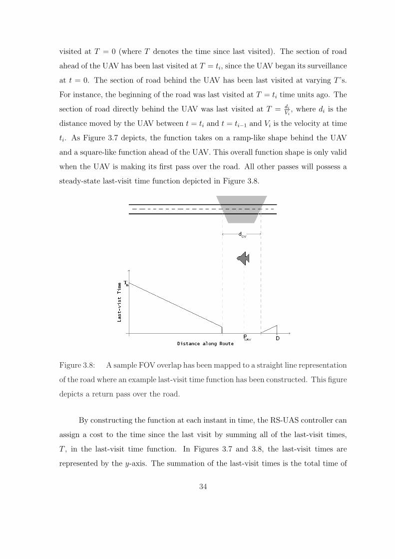
visited at T = 0 (where T denotes the time since last visited). The section of road

ahead of the UAV has been last visited at T = ti, since the UAV began its surveillance

at t = 0. The section of road behind the UAV has been last visited at varying T ’s.

For instance, the beginning of the road was last visited at T = ti time units ago. The

section of road directly behind the UAV was last visited at T = di

Vi, where di is the

distance moved by the UAV between t = ti and t = ti−1 and Vi is the velocity at time

ti. As Figure 3.7 depicts, the function takes on a ramp-like shape behind the UAV

and a square-like function ahead of the UAV. This overall function shape is only valid

when the UAV is making its first pass over the road. All other passes will possess a

steady-state last-visit time function depicted in Figure 3.8.

Figure 3.8: A sample FOV overlap has been mapped to a straight line representation

of the road where an example last-visit time function has been constructed. This figure

depicts a return pass over the road.

By constructing the function at each instant in time, the RS-UAS controller can

assign a cost to the time since the last visit by summing all of the last-visit times,

T , in the last-visit time function. In Figures 3.7 and 3.8, the last-visit times are

represented by the y-axis. The summation of the last-visit times is the total time of

34

last visit to the road. The key to minimizing the revisit time of the UAS to the road

is by effectively driving the overall last-visit time function toward zero. If the road

could be viewed in its entirety at each instant in time, the last-visit time function

would always be zero. In this case, each UAV is traveling the road with a limited

FOV, therefore, the last-visit time function will be manifested as illustrated in Figures

3.7 and 3.8.

The last-visit time function also serves as a convenient method for evaluating

the surveillance along the trajectory and can be re-constructed after PSCOL has

determined the optimal trajectories. Analyzing the resulting last-visit time function

indicates the quality of surveillance on the route. Chapter IV will use this function to

judge the performance of the RS-UAS controller. The next section will demonstrate

how the revisit cost function is calculated using the last-visit time function.

3.6.2 Revisit Cost Function. Before the revisit cost function is developed,

the necessary variables are defined in Table 3.3. The time and state history of the

UAVs, ti and PUAV,i, from the past to the current time are assumed to be known.

Using this information, necessary quantities (defined in Table 3.3) for constructing

the last-visit time function can be calculated for each instant in time. There are two

preliminary steps that help calculate the last-visit time function efficiently.

Table 3.3: Revisit-Cost variable definitionVariable Definition

ti Time history of the vehicle motiontcurrent Current elapsed time since the vehicle began surveillancePUAV,i ith position of UAV in timePA−UAV,i augmented position of UAV in timedOV,i width of ith overlap of FOVPOV vector of distance along the routedroute length of the prescribe routedOV,i FOV overlap on the route at each instant in timeTi Time-since-last-visit history

35

The first step involves augmenting the state position history between the discrete

nodes. Since PSCOL operates with discrete nodes, each UAV’s motion will be assumed

to move in a straight path between position nodes. A linear approximation can be

used to augment the state history, PA−UAV,i. This augmentation process affords higher

resolution when constructing the last-visit time function. The spacing between the

augmented position nodes was chosen to be approximately 200 feet, which is the

minimum FOV overlap (defined as the length of road inside the viewing window of

the camera) on the road when the vehicle is flying wings level. Section 3.5.3 provides

a method for determining the approximate FOV overlaps. Figure 3.9 illustrates a

sample UAV trajectory along a prescribed route with nodes spaced at approximately

200 feet.

Figure 3.9: Sample augmented UAV history along a route.

The second step must translate the route into one dimension (1-D) representing

the distance along the route. The length of the 1-D approximation is the total length

of the prescribed route. This will remove road curvature and provide a method for

determining the FOV overlap on the road at each instant in time. The 1-D represen-

tation is further divided into bins where each bin is also 200 feet in width. POV is a

36

vector where each element represents each 200-foot bin along the route. Simultane-

ously, Ti is a vector the same length as POV where each element represents the time

since last visit for each bin along the route.

Constructing the last-visit time function using the quantities above is done in

several steps. At each point in the augmented state history, the FOV is approximated

and projected onto the ground. The FOV overlap, dOV,i, is determined and translated

to a 1-D distance along the route; there will be a trailing and leading edge point

representing the overlap. The trailing and leading edge points are compared to the

POV vector to find the bins of the route that were overlapped, bins = dOV,i

⋃POV .

Using the overlapped bin element numbers, the time-since-last-visit vector, Ti, is

updated. First, the bin times that were not overlapped are updated with the elapsed

time since the last augmented UAV position, taug. Second, the bin elements that were

overlapped are set to zero.

taug = tcurrent − ti−1 (3.12)

Ti = Ti + taug (3.13)

Ti(bins) = 0 (3.14)

If there is no overlap at the current UAV position, then the time-since-last-visit vector

is updated with taug and no bins are set to zero, and those bins along the route will not

be viewed on the current pass over the route. Figure 3.10 demonstrates an example

of how a route and an FOV overlap map to a single dimension. In the figure, the red

brackets along POV represent the FOV overlap at the current UAV position along the

route. The bins within those brackets correspond to the elements in Ti that are set

to zero in Equation (3.14).

37

Figure 3.10: Sample FOV overlap history translated to a single dimension (dark

flat line). The current overlapped bins are between the red brackets on the route.

The resulting last-visit time function can be illustrated by plotting Ti versus

POV . Figure 3.11 illustrates a sample last-visit time function constructed using the

simulated data in Figure 3.10. The plateaus at Ti = 38, Ti = 35, Ti = 22, and Ti = 0

seconds represent sections of the road that were overlapped simultaneously at the

current time. Those plateaus have varying widths depending on the amount of FOV

overlap, dOV,i. The sharp transition at POV = 0.15 means the plateaus representing

the FOV overlap at Ti = 35 and Ti = 22 covered some of the same area at two

consecutive points in time. Referring back to the reference flight history depicted

in Figure 3.10, the bottom left hand corner shows that some of the FOV trapezoids

did indeed overlap. The square-like waveform ahead of the current overlap at Ti = 0

represents the last-visit time to the route ahead of the current UAV position. Notice

that the height of the square-like waveform is derived from the fact that the route

38

0 0.2 0.4 0.60

5

10

15

20

25

30

35

POV

(mi)

Ti (

s)

Figure 3.11: Sample last-visit time waveform constructed from time and state his-tory depicted in Figure 3.10.

ahead has not been visited. Figure 3.12 demonstrates the last-visit time function

when the UAV has flown further down the route.

0 0.5 1 1.50

20

40

60

80

100

POV

(mi)

Ti (

s)

Figure 3.12: Sample last-visit time waveform from Figure 3.11 propagated in time.

The last-visit time function is ready to be used in calculating the Jrevisit cost

function. The last-visit time vector, Ti, at each UAV position in time, like those

39

illustrated in Figures 3.11 and 3.12, will be summed to produce a revisit time cost for

each UAV. The cooperative nature of the route surveillance mission is captured by

summing Ti across every UAV sector. All the sectors appended together reconstruct

the entire prescribed route. Therefore, summing Ti in this manner assigns a total

revisit cost for the collective team of UAVs. The revisit cost function is given by

Jrevisit =

∫ t(p)M

0

K∑j=1

αji1

Mji

Mi∑i=0

Tji dt (3.15)

where t(p)M is the total time it takes for the UAVs to simultaneously fly one pass over

their sectors of the road, p is the number of phases in the problem (discussed in

Section 3.7.3), Mji is the vector length of Tji, and K is the number of UAVs. The

weighting parameter αji = 1 when there is currently an overlap and αji = c when

there is currently no overlap on the route. The value of c is determined by recording

the amount of UAV positions in the augmented state history that did not have an

FOV overlap on the route. As the UAV diverges from the route, c increases at each

UAV position because the number of times it is missing the route increases. This

weighting scheme adapts to persistent deviations from the route by increasing with

each subsequent non-overlap.

A return pass over the route differs from the development above in the assump-

tion of the last-visit time to the route ahead of the current UAV position. In the

first pass, the time since the last visit was assumed to be the current elapsed time.

However when the UAV has completed a turn and is returning to the origin of the

sector, the time since the last visit is now the last Ti vector for the previous pass. In

other words, the last-visit vector, Ti, is re-used when each UAV returns back down

its sector. The revisit cost function is only one component of JT . The next section

will develop the second portion of RS-UAS controller cost function.

3.6.3 Control Energy Cost Function. The RS-UAS controller cost function

has been augmented with a component to minimize the control energy expended to

40

perform the surveillance. This portion of the performance metric is taken from the

classic linear quadratic regulator cost function. Let the ith UAV’s dynamics modeled

by the autopilot be given by Equation (3.3). Converting VDL,i and φDL,i into state

space

˙VDL,i

˙φDL,i

=

−αV TB 0

0 −αφTB

VDL,i

φi

+

αV TB 0

0 αφTB

V c

DL,i

φci

(3.16)

allows the commanded variables to be gathered into one control vector for the ith

UAV

ui =

V c

DL,i

φci

(3.17)

Therefore, a quadratic cost function form for minimizing the control energy is given

by

Jenergy =

∫ t(p)M

0

uTi Rui dt (3.18)

where t(p)M is the total time for the UAV to complete one pass over the sector. R is

a weighting matrix used to penalize control energy where the weights are selected by

the following expression [27]

Rij = βij1

max(u)2(3.19)

where i = j and βij acts as a tuning gain to penalize the vehicle motion. Equation

(3.18) normalizes the control energy where βij acts to add more or less importance to

the energy minimization. For the simulations in Chapter IV, β was set to unity gain.

Now that the Vehicle Dynamics and Cost Function blocks have been developed, the

next section will explain the methods used to synthesize all of the information into a

multi-phase optimal control problem.

3.7 Problem Setup Block

This section discusses how the inputs from the K-means, Vehicle Dynamics,

and Cost Function blocks are combined into an optimal control problem for PSCOL

41

to solve. Before this problem is presented, the next section demonstrates the methods

for bounding the state dynamics, control inputs, and path constraints. Section 3.7.2

discusses the initial-guess approach used to help PSCOL converge to the optimal

solution. The RS optimal control problem is finally presented in Section 3.7.3.

3.7.1 State, Control, and Path constraint limits. PSCOL requires that all

state, control, and path constraints be restricted before the optimization program

executes. The methods described in this section are for the general case since each

scenario differs. First, the position states defined in the UAV model of Section 3.5.1

are constrained by finding the minimum and maximum value of each UAV sector and

subtracting or adding one mile, respectively. This method constrains the UAV motion

inside an imaginary box around the sector. Although these bounds are necessary for

PSCOL, the distance-from-path constraint keeps them from ever being exceeded.

Figure 3.13 depicts the Texas route divided into four sectors where boxes have been

placed to illustrate state position limits.

0 10 20 30 40 50−6

−5

−4

−3

−2

−1

0

1

2

3

4

5

East (mi.)

Nor

th (

mi.)

Figure 3.13: Example state limits for four sectors.

42

The other aircraft states are bounded using the following methods. The UAV

heading is constrained so that each UAV cannot perform circles during mid-flight.

The only exception is at the ends of the respective sectors. The aircraft velocity, bank

angle, and control inputs are constrained with the values in Table 3.2 to simulate the

performance limits of the TACMAV.

The trajectory of the UAVs around the ends of their respective sectors (repre-

senting the turn-around points) are constrained to a quarter mile East by half mile

North box around the sector endpoints and is illustrated for two sectors in Figure

3.14. Each UAV will not fly outside of this box to complete a turn.

0 2 4 6 8 10 12 14−5

−4.5

−4

−3.5

−3

−2.5

−2

−1.5

−1

−0.5

0

East (mi.)

Nor

th (

mi.)

Figure 3.14: Example turn limits for two sectors.

Table 3.4 lists the path constraint limits used for this research. The commu-

nications limits are taken from the route surveillance mission defined in Chapter I.

The distance-from-path limits are based on projecting the FOV onto the ground and

sweeping the UAV across the route (developed in Section 3.5.3).

Table 3.4: Path constraint limits

Path constraint Min (mi) Max (mi)

Communication limit 0 20

Distance-from-path limit 0 0.2

43

3.7.2 Initial guess. PSCOL requires an initial guess for the optimal control

problem to enhance the solution and to speed-up processing time. In this research,

the initial guess consisted of estimating the UAV trajectories for each sector and

phase. Since a priori knowledge of each sector existed, the UAV trajectories were

approximated by shifting each sector by ∆max = 0.2 miles. While every route is

different, a general initial guess calculation is demonstrated in this section.

Consider the route illustrated in Figure 3.15. The solid colored lines represent

each sector in the route while the initial guess for each sector is shown as dotted lines.

The initial guesses for the first and third phases would take the sector waypoints and

shift them South by ∆max. The initial guess for the second phase takes the sector

waypoints and shifts them North by ∆max. This initial guess method was chosen

because the shifted sectors represent the maximum distance each UAV could travel

from the route and the optimal trajectory should converge within the bound created

by the initial guess. Now that the problem has been bounded and an initial guess has

been determined, the optimal control problem is defined in the next section.

0 5 10 15 20 25−5

−4

−3

−2

−1

0

1

East (mi)

Nor

th (

mi)

Figure 3.15: Example initial guess for two sectors.

3.7.3 PSCOL optimization. The optimal control problem involved in this

research will possess the following multi-phase form. A three-phase approach was

chosen to allow the optimization to account for steady-state operation. The assump-

44

tion is that the second and third passes over the route represent the steady-state

orbit over the respective sectors. Note that the GPM performed by PSCOL outlined

in Section 2.3 always occurs after the following optimal control problem has been

defined. PSCOL will minimize the cost function

JT =3∑

p=1

[J

(p)revisit + J (p)

energy

](3.20)

subject to the dynamics for each UAV in the team as defined by Equation (3.3),

the state boundary conditions presented in Section 3.7.1 and defined in Table 3.2,

the inequality path constraints defined in Equations (3.4) and (3.9), and the phase

linkage constraints

x(psl )(t)− x(ps

u)(t0) = 0, pl, pu = 1, 2, 3; s = 1, 2

t(ps

l )

f − t(ps

u)0 = 0, pl, pu = 1, 2, 3; s = 1, 2 (3.21)

where psl and ps

u are the left and right phases to be connected and s corresponds to

the number of phases being linked (Phase 1 to 2 and Phase 2 to 3). Recall that each

phase corresponds to one UAS pass over the route. Therefore, three phases will allow

the UAS to make three passes over the route. The vehicle dynamics, state boundary

conditions, and inequality path constraints do not change during the three phases.

Note that the form of Jenergy will not change during phase transitions. Jrevisit will

change slightly during phase transitions where the changes are outlined in Section

3.6.2.

3.8 Summary

The RS-UAS controller was developed to provide a solution for dividing pre-

scribed routes and optimizing the UAV trajectories over their respective sectors. The

Input block used methods for creating simulated and real-world routes to test the

controller. The K-means clustering algorithm, the first subcomponent of the con-

45

troller, was applied to the prescribed routes to explore a different method for dividing

routes. The Vehicle Dynamics block uses the TACMAV as the candidate UAV model

for the RS-UAS controller. Also within the Vehicle Dynamics block, the communi-

cations constraint and the distance-from-path constraint are implemented to restrict

the UAV motion to maintain communication with other entities and to ensure the

camera FOV images the route. The RS-UAS controller cost function completes the

RS optimal control problem and was designed to minimize the revisit time to the

route and the overall expended control energy, which achieves the objectives of the

route surveillance mission in Chapter I. The Problem Setup block receives inputs

from the K-means, Vehicle Dynamics, and Cost Function blocks to synthesize the

entire scenario into a three-phase optimal control problem. Chapter IV will present

the results of processing selected route scenarios with the RS-UAS controller.

46

IV. Analysis and Results

4.1 Introduction

This research effort culminates with the results and analysis presented through-

out this chapter. The RS-UAS controller developed in Chapter III was tested by

developing a set of candidate routes that manifested likely urban and rural roadway

characteristics. The metrics used to determine the quality of the solution are mapped

to the following RS mission objectives outlined in Chapter I: determine if the flight

path provides surveillance of the route at all times and determine if the revisit time

of the UAS to the path is minimal. Before the test plan is presented, Section 4.2 will

discuss how the performance metrics are formulated and used to judge performance.

Section 4.3 presents the test plan for the RS-UAS controller and illustrates selected

routes from the test plan. Section 4.4 presents the results from the RS-UAS controller

and analyzes the quality of the solutions.

4.2 Performance Metrics

There are two performance metrics that aid in determining the quality of the

surveillance solutions. The first metric calculates the surveillance coverage for each

phase within a simulation in percent of the route covered, which should be as close

to 100% as possible. The second metric compares the exact travel time of the UAS

to the range of travel times allotted for that phase. Since the RS-UAS cost function

is minimizing more than one aspect of the problem, the revisit time of the UAS is

coupled to the control-energy expenditure. Recall that this research effort is a new

investigation, so the coverage values and revisit times throughout the analysis below

are not compared to previous work, but establish a baseline for any future efforts.

The last-visit time function introduced in Chapter III is the method for deter-

mining the amount of surveillance coverage for each simulation, and is calculated by

recording the amount of the route imaged by the UAS and then dividing by the ap-

propriate route length. Figure 4.1 illustrates an example last-visit time function from

Phase 3 of Simulation 6 in the test plan. Notice that the third sector’s last-visit time

47

function (in red) is a negatively-sloped line representing a sector that was imaged

100%. The other two sectors (magenta and cyan lines) contain spikes corresponding

to sections of the route that were not imaged. This coverage analysis is discussed for

a baseline scenario in Section 4.4, which represents typical results from processing the

test plan.

0 10 20 30 40 500

500

1000

1500

2000

2500

POV

(mi)

Ti (

s)

Figure 4.1: Example last-visit time function from a simulation in the test plan.

In each simulation, the range of travel times was determined by finding the ab-

solute minimum and maximum flight times based on dividing the shortest and longest

sector lengths by the maximum and minimum velocities of the UAVs, respectively.

For example, consider two sectors of a route that are 12 and 12.5 miles in length.

The range of travel times for the two-vehicle UAS would be tmin = 12/Vmax and

tmax = 12.5/Vmin, where Vmin and Vmax are the TACMAV velocity constraints. In

this case, the revisit time to the route in a phase would be minimized when the travel

time of the UAS is tmin.

The revisit time to the route for each phase is equivalent to the travel time of

the UAS. Since Phase 2 and 3 are assumed to represent the steady-state operation,

the revisit times of those phases should settle to a consistent travel time. However,

48

Section 4.4.2 will show that the revisit times do not settle to constant values and

that the minimized control energy of the UAS affects the revisit time by slowing the

vehicles to use less energy. Before the results are presented, the next section will

detail the test plan for the RS-UAS controller.

4.3 RS-UAS Controller Test Plan

The RS-UAS controller was tested by choosing a set of routes from the following

three methods: loading a MATLAB figure and clicking a desired route, generating

a random route, and loading a pre-existing real-world route from Texas. Table 4.1

lists the test plan and the number of nodes used to describe each UAV trajectory per

phase (for example, 30 nodes times 3 phases equals 90 nodes to describe each UAVs

total trajectory). The first two simulations demonstrate how a user can provide a

clicked route to the controller. The sinusoidal-like random route is meant to show

that irregular path shapes (meaning uncommon road shapes) can be processed. Two

versions of the Texas route were used to demonstrate the baseline scenario for the

RS-UAS controller and that the distance-from-path constraint yields better results.

The final clicked route demonstrates a substantial performance increase by doubling

the number of nodes describing each UAV’s total trajectory.

Table 4.1: RS-UAS controller test planSimulation Route Type Team Size Route Length (mi) Nodes

1 Clicked 2 34.58 302 Clicked 4 57.48 303 Random 3 59.86 304 Texas 4 59.81 305 Texas 2 39.94 306 Clicked 3 3 52.34 60

The clicked routes for Simulations 1 and 2 are illustrated in Figures 4.2 and 4.3

and demonstrate the range of complexity for urban and rural environments. Appendix

E contains additional results illustrating the other routes from the test plan, their

49

division, the resulting UAV trajectories, and the last-visit time functions in each

phase.

200 400 600 800 1000 1200

100

200

300

400

500

600

700

(a) Clicked route from map

20 25 30 350

2

4

6

8

10

12

14

16

18

20

East (mi)

Nor

th (

s)

(b) Sectors for each UAV

Figure 4.2: Clicked route from Dayton map and resulting sectors for two UAVs.

200 400 600 800 1000 1200

100

200

300

400

500

600

700

(a) Clicked route from map

0 5 10 15 20 25 30 35 40 450

1

2

3

4

5

6

7

8

9

10

11

East (mi)

Nor

th (

s)

(b) Sectors for each UAV

Figure 4.3: Clicked route from Dayton and resulting sectors for four UAVs.

The test plan in Table 4.1 was successfully executed and the results are presented

in the remaining sections. General concluding remarks about the performance of the

controller are summarized in Section 4.5.

50

4.4 RS-UAS Controller Results

The following sections are organized by discussing each performance metric for

the controller and then the factors that affect those metrics. To minimize the number

of figures and present a concise description of the performance, two tables list the

aggregate surveillance coverage and revisit times for each simulation phase. Also, only

Simulations 4 through 6 are discussed in detail throughout the next two sections. The

surveillance coverage and revisit time results are presented in Sections 4.4.1 and 4.4.2,

respectively. Lastly, Section 4.4.3 demonstrates that the communications constraint

was never violated.

4.4.1 Route Surveillance Coverage. After constructing the last-visit time

function and recording the amount of road imaged for each simulation phase, the

surveillance coverage was calculated and is listed in Table 4.2. The coverage perfor-

mance was only marginal for Simulations 1 through 4, where generally, surveillance

only reached approximately 80% of the route. However, Simulations 5 and 6 show

performance increases because the distance-from-path constraint and the number of

nodes per phase were tuned as a result of analyzing Simulations 1 through 4. Under

the assumptions in Chapter III, the second and third phases offer the best surveillance

trajectories since those are meant to represent steady-state operation. Although the

overall performance in each phase of Simulations 1 through 4 appears marginal, the

coverage across each sector within a phase varied greatly. Since the performance of the

first four simulations are related, only the surveillance coverage results of Simulation

4 (baseline scenario) are discussed in detail.

Under the test-plan conditions in Table 4.1, the RS-UAS controller only provided

surveillance on the Texas route for 67% in Phase 1, 81% in Phase 2, and 82% in Phase

3. Figures 4.4 through 4.6 illustrate the last-visit time functions for Phases 1 through

3, where the horizontal axis is the distance along the route and the vertical axis is the

time since the last visit. Each color-coded section corresponds to the sectors of UAVs

1 through 4, respectively. The best last-visit time function for each phase should be

51

Table 4.2: Surveillance coverage over the route per phase. The processing time foreach simulation is listed in the process column.

Phase 1 Phase 2 Phase 3Simulation Coverage (%) Coverage (%) Coverage (%) Process (hrs)

1 66 63 70 242 65 73 72 303 53 81 82 444 67 81 82 1075 71 84 85 406 94 96 96 43

four negatively or positively-sloped lines depending on the direction of travel (similar

to the example shown in Section 4.2). The frequency of the spikes in the Phase 1

last-visit time function means that the UAS did not image many sections of the route.

Phase 2 increased the amount of surveillance on the route slightly, where each sector

is beginning to contain larger sections that were viewed 100% as compared to Phase

1. In Phase 3, the collective surveillance coverage did increase from the previous

phase, however, there were sections of the route that were never imaged. The spikes

in Figure 4.6 rising to a last-visit time of approximately 3500 seconds correspond to

those areas of the route that were never viewed and for that reason need to be reduced.

The next tier of spikes at last-visit times of approximately 3000 seconds correspond

to sections of the road that have not been viewed since Phase 1, and the final tier

of spikes varying from 1500 to 2000 seconds correspond to sections of the road that

have not been viewed since Phase 2. In spite of this performance, notice that Sector

1 (magenta) of Phase 3 achieved 95% surveillance coverage demonstrating that the

RS-UAS controller provides good results under certain conditions.

52

0 10 20 30 40 500

100

200

300

400

500

600

700

800

POV

(mi)

Ti (

s)

Figure 4.4: Texas road last-visit time function for Phase 1.

0 10 20 30 40 500

200

400

600

800

1000

1200

1400

1600

1800

2000

POV

(mi)

Ti (

s)


53

0 10 20 30 40 500

500

1000

1500

2000

2500

3000

3500

POV

(mi)

Ti (

s)


There are two factors that affect the surveillance coverage performance in Simu-

lations 1 through 4, both of which, consequently, can be compounded resulting in even

worse performance. First, the solutions from PSCOL did not provide good surveil-

lance with 30 nodes describing each UAV trajectory. This meant that PSCOL could

not accurately sample the true optimal solution when the route exhibited complex

transitions. Second, the initial-guess method from Section 3.7.2 in some cases incor-

rectly bounded the potential surveillance trajectory, which is crucial for PSCOL to

find an optimal solution. If these two factors were not present, the surveillance cover-

age reached acceptable levels, as in Sector 1 of Phase 3 for Simulation 4. Since each

factor has been introduced, the remainder of this section will discuss each in detail.

The first and most important factor affecting the quality of the surveillance is the

number of nodes chosen to represent the solution within PSCOL. Recall that PSCOL

is a numerical technique that delivers an approximate solution for optimal control

problems, which Benson et al. [7] showed would approach the exact answer when the

number of nodes N increased. The only method of finding an appropriate number

of nodes is by heuristically determining when the solution is good enough [22, 23].

54

Consequently, since each simulation required at least 24 hours of processing time, the

number of nodes was not increased for Simulations 1 through 5. As an example, a

30th-order Legendre polynomial (corresponding to 30 nodes) was used by PSCOL to

approximate the cost functional, JT . The roots (blue circles) in Figure 4.7 illustrate

the heavy distribution of the points at both ends of the interval [−1, 1], which is a

trait of the Legendre polynomials. When PSCOL converts the solution via the affine

transformation in Equation (2.5), the nodes in the middle of the trajectories can now

be spread over large distances. This is important because the optimal surveillance

trajectories will be improperly sampled during the middle of the trajectory if the

number of nodes is too low. In order to demonstrate improper sampling, Figure 4.8

−1 −0.5 0 0.5 1−0.4

−0.3

−0.2

−0.1

0

0.1

0.2

0.3

0.4

P n(x)

LG Points

Figure 4.7: 30th-order Legendre polynomial used by PSCOL to approximate thesurveillance trajectories of each simulation.

illustrates a sector with transitions that mimic urban roads. Notice that while the

overall trajectories in Figure 4.8(a) appear to provide surveillance, a problem between

miles 12.5 and 14.5 East is illustrated in Figure 4.8(b). There are not sufficient points

to capture the dynamics required to follow the route. This problem is compounded

because this research effort assumed the UAV trajectory between two points was a

straight line. A spline feature in MATLAB could have been used to better approx-

imate the trajectory between the discrete points, but this is left for future work.

55

The maximum surveillance coverage for this sector was only 73% and shows how this

problem affects coverage for complex routes.

12 14 16 18 20 22

2

2.5

3

3.5

4

4.5

5

5.5

East (mi)

Nor

th (

mi)

(a) Sector 2 trajectories for Route 2

12.5 13 13.5 14 14.5 15 15.5

2.8

3

3.2

3.4

3.6

3.8

4

4.2

East (mi)

Nor

th (

mi)

(b) Points for Sector 2 trajectory

Figure 4.8: Sector 2 trajectory for Simulation 2 showing the solution points.

The second quality factor to affect surveillance was the initial-guess method

chosen for this research effort. The surveillance trajectories from PSCOL properly

followed the route when the initial guess correctly bounded the paths taken by the

UAVs. Two examples will demonstrate how a correct and incorrect initial guess

could affect the final surveillance trajectory. Figure 4.9 depicts the Phase 1 and 3

trajectories taken by the first UAV in Simulation 4. Notice that the road moves

mostly in the West-to-East direction. Shifting this sector down by ∆max = 0.2 miles

properly bounded the surveillance trajectory for most of this section (black dotted line

in the figure). However, the portion of road located at mile 10 East is moving nearly

south and never gets viewed by the FOV since the trajectory in the figure overlaps the

route. Overall, the resulting surveillance coverage in this sector improved from 64%

in Phase 1 to 95% in Phase 3. The Sector 1 last-visit time functions (magenta) in

Figures 4.4 through 4.6 illustrate the improved surveillance by the decrease of spikes.

Notice that at POV ≈ 11 miles, the route is missed in all three phases; this corresponds

to mile 10 East on the route.

An incorrect initial guess is depicted in Figure 4.10 (dotted black line) for a

route section that partly moves from South to North. While later sections of this

56

0 2 4 6 8 10 12

−4.5

−4

−3.5

−3

−2.5

−2

−1.5

−1

−0.5

0

East (mi)

Nor

th (

mi)

TrajectoriesRouteInitial guess

Figure 4.9: Simulation 4 initial guess and trajectories for Phase 1 and 3.

sector better conform to the initial-guess method, the middle of the sector does not.

Notice that both of the surveillance trajectories nearly overlap the route above -2 miles

North meaning the FOV is not imaging the route. This is caused because shifting

the route down by ∆max moves the initial guess only South when it should move in

an orthogonal direction from the route by ∆max. This general method caused the

initial guess to nearly overlap the route and did not properly bound the potential

solution. Because later sections of Sector 3 (red) conform to the initial-guess method,

the surveillance coverage, illustrated in Figures 4.4 through 4.6, at the end of the last-

visit time function improved. However, the overall coverage in Sector 3 only increased

from 60% in Phase 1 to 72% in Phase 3. This coverage did not reach the level that

Sector 1 attained because the initial guess was not correct for the entire route.

To counteract the two factors affecting the solution quality, Simulations 5 and

6 were designed to explore two methods that would potentially increase the perfor-

mance of the RS-UAS controller. The first method decreased the distance-from-path

constraint from ∆max = 0.2 miles down to 0.17 miles (forcing the FOV to overlap

regardless of the distance from the route) in order to show that the solution could

57

28 29 30 31 32 33 34 35 36 37−2

−1

0

1

2

3

East (mi)

Nor

th (

mi)

TrajectoriesRouteInitial guess

Figure 4.10: Simulation 4 initial guess and trajectories for Phase 1 and 3.

get better without increasing the number of nodes. The second method, employed in

Simulation 6, doubled the number of nodes to 60 and used a clicked route that mimics

the transitions depicted in Figures 4.8(b), 4.9, and 4.10.

The distance-from-path constraint performed well throughout the simulations

maintaining the UAV trajectories close to the prescribed route, nevertheless, the

adjustability of the ∆max offset provides room for improvement. Simulation 5 used a

portion of the Texas route and decreased the distance-from-path offset down to 0.17

miles. Contrasting Figure 4.11(a) and 4.11(b) to the same route sections in Figures 4.4

and 4.6, demonstrates that decreasing the offset increased the surveillance coverage

for the first 20 miles of the Texas route in Simulation 5 (POV up to 20 miles). Table

4.3 lists the surveillance coverage of the same sections for the two simulations and

demonstrates that all three phases of Simulation 5 were a significant improvement over

Simulation 4. Although performance did increase, this method cannot overcome the

two issues discussed previously. For example, the last-visit time function for Sector

2 (cyan) in Figure 4.11 depicts poor surveillance because this portion of the route

contained sections that moved from South to North.

58

0 5 10 15 20 25 30 350

200

400

600

800

1000

POV

(mi)

Ti (

s)

(a) Phase 1 last-visit time function

0 5 10 15 20 25 30 350

500

1000

1500

2000

2500

3000

3500

4000

POV

(mi)

Ti (

s)

(b) Phase 3 last-visit time function

Figure 4.11: Last-visit time function for Phase 1 and 3 of Simulation 5.

Table 4.3: Results from using smaller ∆max over the first twenty miles of the Texasroute

Phase Simulation 4 Coverage (%) Simulation 5 Coverage (%)

1 67 722 82 903 82 91

By doubling the number of nodes for Simulation 6, the surveillance results were

significantly improved, almost eliminating the effect of the quality factors discussed

previously. The clicked route for Simulation 6 is depicted in Figure 4.12(a), while

Figure 4.12(b) illustrates the resulting trajectory for UAV 3. Notice that the trajec-

tory encapsulates this route better than the similar sector illustrated in Figure 4.10.

Table 4.4 lists the coverage per phase in Simulation 6 and shows that increasing the

nodes helped the surveillance coverage stay above 92%. This means that at maximum

less than one mile out of seventeen was not imaged. Figure 4.1 illustrates the Phase

3 last-visit time function exhibiting no spikes meaning the sector was imaged 100%.

The next section presents results regarding the second performance metric for the

RS-UAS controller.

59

0 10 20 30 40 504

4.5

5

5.5

6

6.5

7

7.5

8

East (mi)

Nor

th (

s)

(a) Clicked route 3

34 36 38 40 42 44 46 48 50

4.5

5

5.5

6

6.5

East (mi)

Nor

th (

mi)

(b) Sector 3 Trajectory

Figure 4.12: Simulation 3 route and resulting Sector 3 trajectory.

Table 4.4: Surveillance coverage for Simulation 3

Sector Sector Length (mi) Phase 1 (%) Phase 2 (%) Phase 3 (%)

1 17.22 97 97 93

2 17.46 93 98 95

3 17.66 92 94 100

4.4.2 Revisit Time. Before the revisit time performance is assessed for

the simulations, it is necessary to compare the travel-time ranges of the UAS to the

travel-time ranges of a single UAV flying the same routes from the test plan. Using

the method for calculating the travel-time ranges from Section 4.2, Table 4.5 lists

the allotted ranges for the UAS (used in PSCOL) and single-UAV cases. The time

variable in this section has been converted to the more convenient time unit of minutes

(10 minutes versus 600 seconds). Note that no extra simulations were processed for

the single-UAV case, so the time ranges for this scenario represent values that would

be used in PSCOL under the same conditions of this research. Recall that the RS

mission in Chapter I called for, in general, at least hourly visits to points along the

route, and in Table 4.5, the single-UAV time ranges are generally hovering around

the one-hour limit for Simulations 2 through 4 and 6 (since those routes are nearly

60

60 miles in length). This suggests that the actual revisit time might fall outside of

the RS-mission requirement. In contrast, the travel-time ranges for the UAS indicate

a benefit since the travel ranges over the route are much less than the hourly visits

required by the RS mission. Table 4.6 lists the actual revisit times for the simulations

from the test plan and demonstrates that the revisit times to the route are well under

the general limit.

Table 4.5: Simulation travel-time ranges for the UAS and single-UAV cases

UAS Single UAV

Simulation Min (min) Max (min) Min (min) Max (min)

1 17 27 34 48

2 14 20 56 79

3 19 31 59 82

4 15 25 59 82

5 20 31 39 55

6 17 27 51 72

Having established that a UAS provides an advantage to the RS mission, the

revisit time performance can be investigated for the simulations from the test plan.

Generally, the revisit times for each phase in Table 4.6 were less than the maximum

travel-time ranges, suggesting that the revisit cost function reduces the revisit time

to the route. In Phase 1 of all the simulations, the revisit time has been minimized

based on the conditions for the minimum travel time in each simulation. However,

the surveillance coverage for Phase 1 is poor (except for Simulation 6) as listed in

Table 4.2 from Section 4.4.1. In all cases, the revisit time increases for Phases 2 and 3

while the surveillance coverage and control-energy expenditure improve. Figure 4.13

illustrates the normalized control energy during each phase of Simulation 6 (color

coded) and shows that the revisit time is coupled to the control energy expended by

the UAS. Notice that the control energy is highest in Phase 1, which is expected since

61

the revisit time is shortest. The spikes at t = 17 min and t = 40 min correspond to

the turn-around points at the end of the sectors.

Table 4.6: Simulation revisit times for each phasePhase 1 Phase 2 Phase 3

Simulation Travel (min) Travel (min) Travel (min)

1 17 21 252 14 20 203 19 25 294 15 22 235 20 23 266 17 24 24

0 10 20 30 40 50 601

1.2

1.4

1.6

1.8

2

2.2

2.4

2.6

2.8

3

Time (min)

Nor

mal

ized

Con

trol

Ene

rgy

Figure 4.13: Simulation 6 control energy minimization.

In Phases 2 and 3, the revisit times, along with the surveillance coverage and

control energy, should settle from a transient-like behavior to a steady-state operation.

The two main factors affecting the RS-UAS controller performance were discussed in

the previous section and also largely contribute to the unsettled revisit times for

Phases 2 and 3. Specifically, the revisit cost function records the last time portions

of the route were visited, however, if the surveillance is sporadic, like Simulations 1

62

through 4, the revisit time will not settle to a constant value. Doubling the nodes

in Simulation 6, mitigated the affect of those performance factors on the surveillance

coverage as well the revisit time since it settled to a steady-state of 24 minutes. Even

though performance improved in the last simulation, the revisit time in Phase 1 is

much shorter, which is also common to the first five simulations.

The performance in Phase 1 can be attributed to improper weighting in the

first phase of the RS-UAS cost function. Recall that the c parameter in the revisit

cost and the β parameter in the control-energy cost seek to place an appropriate

importance on the two portions of the overall RS-UAS cost function. Consequently,

there is a weighting struggle between the two portions of the cost function. Globally,

this weighting issue is overshadowed by the two quality factors in the previous section,

and Simulation 6 shows that once those issues are mitigated the revisit time settled

appropriately. The next section will briefly discuss the communications constraint

before this chapter is summarized in Section 4.5.

4.4.3 Communications Constraint. The communications constraint was

never violated throughout the simulations because the routes were properly divided

by the K-means clustering algorithm. If the sectors had been unbalanced, the commu-

nications constraint would have been violated. Simulation 5 approached the constraint

because the sector lengths were close to the 20-mile limit. The peak distance between

the two UAVs was 19 miles in phase two. Figure 4.14 illustrates the communications

spacing throughout each phase for the two UAVs.

63

0 500 1000 1500 2000 2500 3000 3500 40000

2

4

6

8

10

12

14

16

18

20

Time (s)

Com

mSp

acin

g (m

i)

Phase 1Phase 2Phase 3

Figure 4.14: Communications spacing between UAV 1 and 2 for Simulation 6.

4.5 Summary

The results outlined in Tables 4.2 and 4.6 demonstrate that the RS-UAS con-

troller performed marginally until the number of nodes was doubled in Simulation 6.

The first four routes in the test plan were not provided with persistent surveillance

also causing the revisit time not to settle to a constant value. However, the analysis

revealed that the number of nodes chosen to represent the surveillance trajectories

and the initial-guess method of Section 3.7.2 significantly influenced the quality of the

solution. The distance-from-path constraint was found to have a less significant im-

pact on the solution. Chapter V will summarize this research effort, suggest methods

to improve the RS-UAS controller, and propose options for future research.

64

V. Conclusions and Recommendations

This chapter summarizes the research effort used to solve the route surveillance prob-

lem. The summarized results are drawn upon to recommend future work intended

to improve the RS-UAS controller and take this research beyond the assumptions in

Chapter I.

5.1 Conclusions

The primary objective of this research was to apply optimal control theory

and cooperative control theory to allow a four-vehicle UAS to provide persistent

surveillance of a roadway. The route surveillance UAS objectives were to minimize the

revisit time to points along the route and to maximize the flight time of the system

without losing surveillance. The control algorithm was required to automatically

adjust to changes in the number of UAVs to create a pattern such that each vehicle

maintains surveillance of the route and the ability to communicate with the other

entities in the system.

By applying general approaches from the current cooperative search literature,

the RS-UAS controller provided a method for dividing the waypoint-defined route

and, more importantly, a method for developing surveillance trajectories to ensure the

camera FOV imaged the road. Using the number of UAVs and the route as inputs, the

controller autonomously adds resolution to the route as necessary, dissects the route

using the K-means clustering algorithm, and constructs an optimal control problem

that is solved by the GPM-based optimization software. In order to complete the RS

optimal control problem, the overall problem objectives were translated into a cost

function and two path constraints. The cost function was developed to minimize the

revisit time along the route and the overall control energy of the UAS. Two path

constraints restricted the distance between entities and the distance of each UAV

from the route. The RS optimal control problem was synthesized into a three-phase

optimal control problem compatible with PSCOL, where each phase would represent

one collective pass of the UAS over the route.

65

Using three methods to supply candidate routes, a test plan was created to

demonstrate the controller through processing simulated and real-world routes that

mimicked urban and rural environments. Two performance metrics ascertained that

persistent surveillance coverage was delivered and that the revisit time to the route

was reduced. The last-visit time function used to calculate the revisit cost also doubled

as a tool to determine the quality of the surveillance. The UAS travel time in each

simulation was compared to the single-UAV case to show that the revisit time met

the general one-hour requirement of the RS mission. Once the travel-time ranges for

each simulation were established, the revisit time in each phase was compared to the

maximum allowed travel time to check the revisit time performance.

Results showed that the RS-UAS controller did not provide persistent surveil-

lance in the first four simulations. An analysis of the last-visit time function and

resulting UAV trajectories revealed two factors that significantly influenced the qual-

ity of the solution. The crucial factor was the number of nodes representing the

optimal solution from PSCOL, which posed problems because of the heavy distribu-

tion of the points at the two ends of the sector. If the sector had complex transitions

in the middle of the route, the solution became sensitive to the number of nodes. The

second factor revealed that PSCOL required an initial guess that bounded the poten-

tial surveillance trajectory. If the guess was adequate, surveillance reached acceptable

levels. But when the guess was inadequate, the route was not imaged consistently.

Both of these factors contributed to marginal results, however, further analysis did

show that the controller could provide good results.

Two methods were tested to determine if performance could be increased in the

last two simulations. The first approach decreased the distance-from-path constraint

while holding the number of nodes constant. Performance did increase in a limited

case, but the distance-from-path constraint is not an approach to overcome the two

issues regarding the number of nodes and the initial guess. The second approach

doubled the number of nodes in Simulation 6, which used a route that was similar

to sections from the first five simulations. The overall surveillance coverage reached

66

96% of the route and the revisit time to the route settled to a steady-state value as

expected. These results indicate that the approach used in the RS-UAS controller

can provide feasible solutions for the route surveillance problem.

In summary, applying optimal control to the route surveillance problem is an

appropriate solution method. The cost function and path constraints developed in this

research demonstrate that formulating an optimal control problem can provide feasible

results. Their potential was realized in only two of the six simulations because of issues

specific to the numerical optimization software chosen for this research. Future work is

encouraged in order to improve and extend the application of optimal control theory

to the route surveillance problem. The next section will suggest avenues of future

work to improve upon this new research area.

5.2 Future Research

There are two directions for improving upon this research effort. The first di-

rection is aimed at improving the quality of the solutions provided by the current

RS-UAS controller. The second direction concentrates on expanding this research’s

problem statement to include realistic assumptions about the route surveillance mis-

sion.

The most significant improvements to the controller developed in this research

would be to investigate the feasibility of increasing the number of nodes during simu-

lations and develop a better method for providing a general initial guess to PSCOL.

Karasz [23] used an iterative method to quickly solve for the appropriate number of

nodes in his application of the GPM. Perhaps, an appropriate distribution of points

can be found by iteratively increasing the order of the Legendre polynomials and

fitting the location of the roots to the current route under consideration. A better

guess allows PSCOL to provide enhanced optimal solutions, therefore, a method that

bounds the solution for any route shape should help PSCOL quickly find an accurate

solution.

67

Future work in this area could also take one phase describing a complex sector

and split it into multiple phases to increase resolution for that sector. This approach

could potentially alleviate the need for increasing the number of nodes per phase

(increasing the processing time) and a better initial guess (assuming that the new

sectors would be less complex).

The research problem statement in Chapter I addressed a limited portion of the

route surveillance mission. Expanding several components of the problem statement

opens a whole range of possible future research. First, the candidate routes considered

in this research did not include terrain or urban development. The UAVs are assumed

to fly at a range of 300 ft above ground level. Mountainous terrain, city buildings,

and tall trees in forests could potentially impact the UAV trajectory along the route

or impede the camera’s view of the route. Future research should expand the route

definitions to include environment characteristics other than path shape.

Second, the UAV model and UAS composition are another area to focus future

research. The largest limiting assumption of the UAV model in this research is the

absence of wind. Even adding constant wind to the problem adds another dimension

of complexity. The UAV model should be extended to account for deterministic or

stochastic wind models. The first-order UAV model in this research contained a

simplified set of states and controls, but model fidelity should be extended to include

3-DOF and 6-DOF models depending on the required level of accuracy. Also, the

UAS could be extended to included a heterogeneous team of UAVs that possesses a

sensor suite tailored for all types of mission environments, day or night.

Third, the ranges of the routes in this research made a hardware simulation

difficult within the test range available to AFIT. In conjunction, UAVs available for

academic research at AFIT possess limited maximum flight times depending on the

aircraft. Future research could consider decreasing the length of the prescribed routes

to fit within a reasonably sized test range to allow multiple passes over the route to be

68

within the flight times of available UAVs. Performing hardware tests would validate

any surveillance trajectories developed by a controller.

Lastly, the problem statement constrained the complexity in the problem to

local coupling. Reshaping the mission within the current objectives would certainly

lead to a higher degree of coupling between UAV decisions, mission tasks, and mission

outcomes. Depending on the amount of coupling, future research could contrast the

application of both a centralized and decentralized control approach. In the decen-

tralized case, current cooperative search solutions could be applied to that research

effort. This comparison between control architectures could also significantly impact

any operational implementation.

69

Appendix A. Dimensionless UAV model

PSCOL offers an automatic scaling option for optimal control problems. In practice,

the automatic scaling has been found to be useful, but it is recommended by the

authors of PSCOL to scale and non-dimensionalize the optimal control problem prior

to using any numerical technique. Badly scaled problems can cause the software to

conclude with infeasible solutions or to continue searching for a non-existent solution.

The equations of motion outlined below are badly scaled in the size of the position,

velocity, and time values. The dimensionless equations of motion will ensure val-

ues between zero and one for the position and velocity states as well as the system

time. The equations chosen for modeling the UAV flight dynamics are a first-order

approximation and are given by

pN,i = V cosψi + wN (A.1)

pE,i = V sinψi + wE (A.2)

ψi =g

Vi

tan φi (A.3)

Vi = αV (V ci − Vi) (A.4)

φi = αφ(φci − φi) (A.5)

where i = 1, ..., N and N is the number of UAVs. The above equations will be

non-dimensionalized first for the i = 1 general case using the following relationships:

VDL =V

Vmax

(A.6)

p′N =pN

PRT

(A.7)

p′E =pE

PRT

(A.8)

τ =t

TB

(A.9)

70

V cDL =

V c

Vmax

(A.10)

The subscript DL and the prime superscript are defined as the dimensionless vari-

ables. The velocity state and control velocity of each UAV will be scaled and non-

dimensionalized by the maximum velocity. The northing and easting positions will

be scaled and non-dimensionalized by the maximum route length of 60 miles. Time

must also be scaled and non-dimensionalized due to the possibly long flight times,

therefore, the scaling factor will be the period of revisit to the route. Notice that

heading and roll angle are dimensionless already. The dimensionless time differential

operator must be derived first. The derivation begins by considering the relationship

t = TBτ

dt = TBdτ

dτ

dt=

1

TB

(A.11)

The dimensionless differential operator is derived by using the derivative chain rule.

d

dt=

dτ

dt

d

dτd

dτ=

dt

dτ

d

dt=⇒ TB

d

dt(A.12)

The dimensionless equations of motion can now be derived.

Northing position:

d

dτ(p′N) = TB

d

dt

(pN

PRT

)

=TB

PRT

pN

=TB

PRT

[V sin ψ]

p′N =TB

PRT

VDLVmax sin ψ (A.13)

71

Easting position:

d

dτ(p′E) = TB

d

dt

(pE

PRT

)

=TB

PRT

pE

=TB

PRT

[V sin ψ]

p′E =TB

PRT

VDLVmax cos ψ (A.14)

Heading:

d

dτ(ψ) = TB

d

dt(ψ)

= TBψ

= TB[g

Vtan φ]

ψND =gTB

VDLVmax

tan φ (A.15)

Velocity:

d

dτ(VDL) = TB

d

dt

(V

Vmax

)

=TB

Vmax

V

=TB

Vmax

[αV (V ci − Vi)]

VND = αV TB(V cDL − VDL) (A.16)

Roll rate:

d

dτ(φ) = TB

d

dt(φ)

= TBφ

= TB[αφ(φci − φi)]

φND = αφTB(φc − φ) (A.17)

72

Therefore, the scaled and non-dimensionalized equations of motion for the ith UAV

are given by

p′N,i =TBVmax

PRT

VDL,i sin ψi

p′E,i =TBVmax

PRT

VDL,i cos ψi

ψDL,i =gTB

Vmax

tan φi

VDL,i

VDL,i = αV TB(V cDL,i − VDL,i)

φDL,i = αφTB(φci − φi) (A.18)

73

Appendix B. Camera Field-of-View Approximation

Using Terning’s work [33] as a reference, equations were developed to approximate

the sensor footprint projected onto the ground. These relationships will be used to

determine suitable equations for the camera FOV overlap on the prescribed path. The

following figure will be used for reference throughout the development. In order to

calculate the quantities from the equations below, information about the aircraft alti-

tude and attitude must be known. Also, information regarding the camera elevation

angle, azimuth angle, and camera FOV must be known.

Figure B.1: Camera Field-of-View depiction taken from [33]

In the lefthand image, the Linefwd and Linerear of the sensor footprint are given

by

Linefwd =hUAV

tan(θcamElevation − Φ− θV ertCamFOV

2)

(B.1)

Linerear =hUAV

tan(θcamElevation − Φ + θV ertCamFOV

2)

(B.2)

where Φ represents vehicle pitch or vehicle roll depending on approximating the for-

ward or side looking camera FOV (this is the modification to Terning’s research).

Using Equations (B.1) and (B.2), the corners can be calculated by the following

equations for the quantities depicted in Figure B.2. Although the forward-looking

case is illustrated, Equations (B.3)-(B.5) are also valid for the side-looking camera

74

FOV approximation.

Rfwd =√

h2UAV + Line2

fwd (B.3)

Camfwd−LHS = Rfwd tan(θHorizCamFOV

2) (B.4)

Camfwd−RHS = −Rfwd tan(θHorizCamFOV

2) (B.5)

Figure B.2: Camera Field-of-View corner depiction taken from [33]

Listing B.1: This MATLAB function is a modified version of Terning’s functionused to approximate the camera FOV.

function [flines ,FOVPLOT ] = createFOV(x_u , y_u , hdg_u ,roll , alt_u..., camAngle , camElevation , Horiz_camFOV ,Vert_camFOV , fieldlimit ..., plotflag)

%createFOV provides trapezoidal representation of UAV sensor FOV% Currently does account for bank angle.% All angles should be in radians

5 % This version accounts for horizontal and vertical FOV angles%% Fieldlimit variable needs to be defined in order to scale the ...

FOV appropriately within PSCOL

camElevation_c = camElevation - roll; % Correct the camElevation...to account for the bank angle

10 d2r = pi/180;

up = max(camElevation_c - Vert_camFOV /2,0);flines = [ alt_u/tan(camElevation_c + Vert_camFOV /2) , alt_u/tan(up)...

]; % Line_REAR and Line_FWD

15 if abs(flines (2))>fieldlimit ,flines (2)=fieldlimit;

end

75

range = [ norm([ flines (1),alt_u ]) , norm([ flines (2),alt_u ])]; ...% R_rear & R_fwd : Distance from UAV to the ...

Line_REAR and Line_FWD20 fRH = [- range (1)*tan(Horiz_camFOV /2) , -range (2)*tan(Horiz_camFOV...

/2)]; % Back and Front CAM_RHSfLH = [ range (1)*tan(Horiz_camFOV /2) , range (2)*tan(Horiz_camFOV /2)...

]; % Back and Front CAM_LHSffarlength = abs(fRH(2) - fLH(2));fnearlength = abs(fRH (1) - fLH (1));hyp = [ norm([ fnearlength /2,range (1)]) , norm([ ffarlength /2,range (2)...

])];25

%Rotate above shape to desired heading/camera angle combinationrfar = norm([fRH (2),flines (2)]); %projected radial distance to far...

ptrnear = norm([fLH(1),flines (1)]); %projected radial distance to ...

near ptranglefar = atan2(fRH (2),flines (2));

30 ranglenear = atan2(fRH(1),flines (1));ranglefar2 = [- ranglefar+camAngle+hdg_u , ranglefar+camAngle+hdg_u...

];ranglenear2 = [- ranglenear+camAngle+hdg_u , ranglenear+camAngle+...

hdg_u ];FOV1 = [ x_u+rfar*cos(ranglefar2 (2)),(y_u+rfar*sin(ranglefar2 (2)))...

];%top RH

35 FOV2 = [ x_u+rfar*cos(ranglefar2 (1)) , (y_u+rfar*sin(ranglefar2 (1)))...];

%top LHFOV3 = [ x_u+rnear*cos(ranglenear2 (2)) , y_u+rnear*sin(ranglenear2...

(2))];%bottom LHFOV4 = [ x_u+rnear*cos(ranglenear2 (1)) , y_u+rnear*sin(ranglenear2...

(1))];40 %bottom RH

FOVPLOT =[FOV1;FOV2;FOV4;FOV3;FOV1];

return %createFOV

76

Appendix C. K-means Clustering Algorithm

Listing C.1: K-means clustering algorithm from Mathworks File Exchange [11].function [gIdx ,c]= k_means(X,k)% K_MEANS k-means clustring% IDX=k_means(X, K) partitions NxP matrix X into K clusters% using fully vectorized algorithm , where N is number of data

5 % points and P is number of variables . The partition minimizes% sum of point -to -cluster -centroid Euclidean distances of all% clusters . The returned Nx1 vector IDX contains the cluster% indices of each point.% IDX = k_means(X, C) works with the initial centroids ,C,(K x P).

10 % [IDX ,C]= k_means(X, K) returns K centroid locations in KxP ...matrix ,C.

% Version 2.0, by Yi Cao at Cranfield University on 27 March 2008.

% Check input and outputerror(nargchk (2,2,nargin));

15 error(nargoutchk (0,2,nargout));

[n,m]=size(X);

% Check if second input is centroids20 if ~ isscalar(k)

c=k; k=size(c,1);else

c=X(ceil(rand(k,1)*n) ,:);end

25% allocating variablesg0=ones(n,1); gIdx=zeros(n,1); D=zeros(n,k);

% Main loop converge if previous partition is the same as current30 while any(g0~=gIdx)

g0=gIdx;% Loop for each centroidfor t=1:k

d=zeros(n,1);35 % Loop for each dimension

for s=1:md=d+(X(:,s)-c(t,s)).^2;

endD(:,t)=d;

40 end% Partition data to closest centroids[z,gIdx]=min(D,[],2);% Update centroids using means of partitionsfor t=1:k

45 c(t,:)=mean(X(gIdx==t,:));end

end

77

Appendix D. Dudek’s Taxonomy

This appendix will provide an overview of Dudek’s taxonomy used to facilitate the

discussion of multi-agent robotic properties, in this case the RS-UAS. “A key difficulty

in the design of multi-agent robotic systems is the size and complexity of the space

of possible designs. In order to make principled design decisions, an understanding of

the many possible system configurations is essential” [16].

The collective size property categorizes the number of entities acting collabo-

ratively within the environment. A group of autonomous vehicles can range from

a single entity to many entities. SIZE-ALONE and SIZE-PAIR are groups of one

and two entities, respectively, while SIZE-LIM refers to groups of two or more enti-

ties. Dudek included a SIZE-INF category to account for large group numbers that

saturate the goals or the environment under consideration.

Communication range applies to entities communicating with other group mem-

bers, but does not apply to entities communicating with human operators. The COM-

NONE category defines a situation when there is no communication between entities.

COM-NEAR represents situations when the communication range is limited by hard-

ware or environment. COM-INF assumes there is no limit to communication range

but really describes scenarios where the range is much greater than the environment

of operation.

Communication topology refers to the manner in which the entities communicate

or broadcast information to the rest of the group. TOP-BROAD categorizes situations

where an entity can broadcasts to other group members within range. TOP-ADD

refers to a topology that uses unique identifiers to send information to the entity

being identified. This is similar to a computer network using Internet Protocol (IP)

addresses to send information to unique computers. TOP-TREE describes topologies

that use a static tree communication scheme and, similarly, TOP-GRAPH categorizes

scenarios that use a graph topology. Note that the broadcast topology is the most

robust scheme since it is not dependent on a single agent passing information.

78

Communication bandwidth describes how much information can be transmit-

ted for direct and indirect communication. The information transmitted throughout

the group carries with it an associated cost for communication, i.e. enemy intercep-

tion. BAND-ZERO assumes that no communication is possible and therefore dictates

that there is no achievable cooperation. BAND-LOW categorizes situations when the

communication is highly restrictive due to high consequences of enemy interception.

“BAND-MOTION is used to describe network architectures that consider communi-

cation cost to be of the same order of magnitude of the cost of moving the robot

between locations” [19]. BAND-INF describes scenarios when the communication

cost is insignificant.

Collective reconfigurability describes how fast the group can reconfigure it-

self spatially within the environment. ARR-STATIC describes situations where the

group’s configuration is not changing over time. ARR-COM categorizes groups that

reconfigure due to cooperation being dependent on communication between entities.

ARR-DYN refers to groups that reconfigure indiscriminately.

Processing ability refers to classification of the computational model used by the

entities in the group. PROC-SUM processing is a simple non-linear summation while

PROC-FSA assumes entities use the finite-state automata. PROC-PDA describes

entities that use the push-down automata computation method. PROC-TME is the

most common computation method and uses the Turning Machine equivalent.

The final property in Dudek’s Taxonomy is group composition both in the sense

of software and hardware. CMP-IDENT describes groups of entities that are all identi-

cal, while CMP-HOM refers to groups of entities that only differ in the software being

used for control. CMP-HET is a category for groups of entities that are physically

different in capabilities, on-board sensors, or both.

Dudek’s Taxonomy is a tool for analyzing an intended system in a CC problem.

Table D.1, which was reproduced from [19], concisely outlines Dudek’s Taxonomy.

79

Table D.1: Dudek’s TaxonomyProperty Description Subdivision

Collective Size The number of autonomous agents inthe collective

SIZE-ALONESIZE-PAIRSIZE-LIMSIZE-INF

Communicationsrange

The max distance between 2 elements ofthe collective such that communicationsis valid

COM-NONECOM-NEARCOM-INF

Communicationtopology

The topology used when elements com-municate within the range

TOP-BROADTOP-ADDTOP-GRAPHTOP-TREE

Communicationbandwidth

How much information can elementstransmit to each other collective

BAND-ZEROBAND-LOWBAND-MOTIONBAND-INF

Collective recon-figurability

The rate at which the collective canspatially reorganize itself

ARR-STATICARR-COMARR-DYN

Processing ability The computational model used by indi-vidual elements of the collective

PROC-SUMPROC-FSAPROC-PDAPROC-TME

Collective compo-sition

Are the elements of the collective ho-mogeneous or heterogeneous

CMP-IDENTCMP-HOMCMP-HET

80

Appendix E. Additional Results

This appendix provides additional results from the six simulations outlined in the test

plan of Section 4.3. They are given in the same order as presented in Table 4.1.

E.1 Clicked Route 1

Figure E.1 illustrates the first clicked route from a Dayton area map and the

resulting sectors. Figure E.2 illustrates the resulting trajectories from the PSCOL

simulations.

200 400 600 800 1000 1200

100

200

300

400

500

600

700

(a) Clicked path from map

20 25 30 350

2

4

6

8

10

12

14

16

18

20

East (mi)

Nor

th (

s)

(b) Resulting sectors

Figure E.1: Clicked route from Dayton for two UAVs and the resulting sectors.

17 18 19 20 21 22 23 24 25 260

1

2

3

4

5

6

7

8

9

10

East (mi)

Nor

th (

mi)

(a) Sector 1 Trajectory

28 30 32 34 36

11

12

13

14

15

16

17

18

19

East (mi)

Nor

th (

mi)


Figure E.2: Sector trajectories over clicked Dayton road.

81

Figures E.3-E.5 depict the last-visit time functions during the three phases of

the problem.

0 5 10 15 20 25 300

100

200

300

400

500

600

700

800

900

1000

1100

POV

(mi)

Ti (

s)

Figure E.3: Clicked Road 1 last-visit time function for Phase 1.

0 5 10 15 20 25 300

500

1000

1500

2000

POV

(mi)

Ti (

s)


82

0 5 10 15 20 25 300

500

1000

1500

2000

2500

3000

3500

POV

(mi)

Ti (

s)


Table E.1 lists the coverage percentage during each phase for both sectors of

the route.

Table E.1: Surveillance coverage for Clicked Route 1


1 17.29 79 69 68

2 17.29 54 56 72

E.2 Clicked Route 2

Figure E.6 illustrates the second clicked route from a Dayton area map and the

resulting sectors. Figure E.7 illustrates the resulting trajectories from the PSCOL

simulations.

83

200 400 600 800 1000 1200

100

200

300

400

500

600

700

(a) Clicked path from map

0 5 10 15 20 25 30 35 40 450

1

2

3

4

5

6

7

8

9

10

11

East (mi)

Nor

th (

s)

(b) Resulting sectors

Figure E.6: Clicked route from Dayton for four UAVs and the resulting sectors.

84

2 3 4 5 6 7 8 9 10 110

1

2

3

4

5

6

East (mi)

Nor

th (

mi)


12 14 16 18 20 22

2

2.5

3

3.5

4

4.5

5

5.5

East (mi)

Nor

th (

mi)


24 26 28 30 32

2.5

3

3.5

4

4.5

5

5.5

6

6.5

East (mi)

Nor

th (

mi)

(c) Sector 3 Trajectory

34 36 38 40 42 44

3

4

5

6

7

8

9

10

11

East (mi)

Nor

th (

mi)

(d) Sector 4 Trajectory

Figure E.7: Sector trajectories over clicked Dayton road for 4 UAV case.

Figures E.8-E.10 depict the last-visit time functions during the three phases of

the problem.

85

0 10 20 30 40 500

100

200

300

400

500

600

700

800

POV

(mi)

Ti (

s)


0 10 20 30 40 500

200

400

600

800

1000

1200

1400

1600

1800

2000

POV

(mi)

Ti (

s)


86

0 10 20 30 40 500

500

1000

1500

2000

2500

3000

POV

(mi)

Ti (

s)


Table E.2 lists the coverage percentage during each phase for both sectors of

the route.



1 14.19 68 88 87

2 14.52 73 76 63

3 14.29 64 70 72

4 14.48 55 57 65

E.3 Random Route 1

Figure E.11 illustrates a random route divided into three sectors. This route was

used for two scenarios where each differed in the implementation of the cost function.

The first scenario explained in this section minimized revisit time and control energy.

Figure E.12 illustrates the trajectories for each UAV.

87

0 5 10 15 20 25 30 350

2

4

6

8

10

12

14

16

18

20

East (mi)

Nor

th (

s)

Figure E.11: Random road divided into three sectors.

0 1 2 3 4 52

4

6

8

10

12

14

East (mi)

Nor

th (

mi)


6 8 10 12 14 16 18

9

10

11

12

13

14

15

16

17

18

19

East (mi)

Nor

th (

mi)


20 22 24 26 28 30 32 34

12

14

16

18

20

22

East (mi)

Nor

th (

mi)


Figure E.12: Sector trajectories over random road for 3 UAV case.

88

The last-visit time functions for each phase are illustrated in Figures E.13-E.15.

0 10 20 30 40 500

200

400

600

800

1000

POV

(mi)

Ti (

s)

Figure E.13: Random road last-visit time function for Phase 1.

0 10 20 30 40 500

500

1000

1500

2000

2500

POV

(mi)

Ti (

s)


89

0 10 20 30 40 500

500

1000

1500

2000

2500

3000

3500

4000

POV

(mi)

Ti (

s)


Surveillance coverage per phase outlined in Table E.3.

Table E.3: Surveillance coverage for random route


1 19.77 38 86 42

2 20.04 76 85 50

3 19.91 56 97 58

E.4 Texas Route 1

The Texas route served as the baseline scenario for the RS controller. Results

were acceptable, but could have been better. The resulting sectors for four UAVs are

depicted in Figure E.16.

90

0 10 20 30 40 50−5

−4

−3

−2

−1

0

1

2

3

4

POV

(mi)

Ti (

s)

Figure E.16: Texas road divided into four sectors.

Figure E.17 depicts the UAV trajectories over their respective sectors.

91

0 2 4 6 8 10 12

−4.5

−4

−3.5

−3

−2.5

−2

−1.5

−1

−0.5

0

East (mi)

Nor

th (

mi)


14 16 18 20 22 24 26

−4.5

−4

−3.5

−3

−2.5

−2

−1.5

−1

East (mi)

Nor

th (

mi)


28 29 30 31 32 33 34 35 36 37−2

−1

0

1

2

3

East (mi)

Nor

th (

mi)


38 40 42 44 46 48 50 52

2.4

2.6

2.8

3

3.2

3.4

3.6

East (mi)

Nor

th (

mi)

(d) Sector 4 Trajectory

Figure E.17: Sector trajectories over Texas road.


92

0 10 20 30 40 500

100

200

300

400

500

600

700

800

POV

(mi)

Ti (

s)

Figure E.18: Texas road last-visit time function for Phase 1.

0 10 20 30 40 500

200

400

600

800

1000

1200

1400

1600

1800

2000

POV

(mi)

Ti (

s)


93

0 10 20 30 40 500

500

1000

1500

2000

2500

3000

3500

POV

(mi)

Ti (

s)


Table E.4: Surveillance coverage for Texas route


1 14.72 65 80 95

2 14.81 78 85 80

3 14.99 60 80 72

4 15.29 70 80 80

E.5 Texas Route 2

This simulation only used a portion of the Texas route because the UAS con-

sisted of only two UAVs. The distance-from-path constraint was decreased in this sim-

ulation, and results show that in Sector 1 surveillance coverage increased. However,

Sector 2 contained a section that did not conform well to the initial-guess method,

and therefore the coverage was marginal. The resulting sectors for two UAVs are

depicted in Figure E.21.

94

0 5 10 15 20 25 30

−4

−3

−2

−1

0

1

2

3

East (mi)

Nor

th (

s)

Figure E.21: Partial Texas road divided into two sectors.


0 2 4 6 8 10 12 14 16

−4.5

−4

−3.5

−3

−2.5

−2

−1.5

−1

−0.5

0

East (mi)

Nor

th (

mi)


18 20 22 24 26 28 30 32

−2

−1

0

1

2

3

4

East (mi)

Nor

th (

mi)


Figure E.22: Sector trajectories over Simulation 2.


95

0 5 10 15 20 25 30 350

200

400

600

800

1000

POV

(mi)

Ti (

s)


0 5 10 15 20 25 30 350

500

1000

1500

2000

2500

POV

(mi)

Ti (

s)


96

0 5 10 15 20 25 30 350

500

1000

1500

2000

2500

3000

3500

4000

POV

(mi)

Ti (

s)


Table E.5: Surveillance coverage for partial Texas route


1 19.93 84 90 91

2 20.01 60 78 80

E.6 Clicked Route 3

This third clicked route served as the simulation that investigated raising the

number of nodes to sixty. While the performance was of high quality, a section of the

route in Sector 2 did not conform well to the initial-guess method. As a result, there

were some sections of the route that were missed in Phases 1 and 3. The resulting

sectors for three UAVs are depicted in Figure E.26.

97

0 10 20 30 40 504

4.5

5

5.5

6

6.5

7

7.5

8

East (mi)

Nor

th (

s)

Figure E.26: Clicked Route 3 divided into three sectors.


98

0 2 4 6 8 10 12 14 16

5.5

6

6.5

7

7.5

8

East (mi)

Nor

th (

mi)


16 18 20 22 24 26 28 30 324.4

4.6

4.8

5

5.2

5.4

5.6

5.8

6

6.2

6.4

East (mi)

Nor

th (

mi)


34 36 38 40 42 44 46 48 50

4.5

5

5.5

6

6.5

East (mi)

Nor

th (

mi)


Figure E.27: Sector trajectories over Clicked Route 3.


99

0 10 20 30 40 500

100

200

300

400

500

600

700

800

900

1000

POV

(mi)

Ti (

s)

Figure E.28: Clicked Route 3 last-visit time function for Phase 1.

0 10 20 30 40 500

500

1000

1500

2000

POV

(mi)

Ti (

s)


100

0 10 20 30 40 500

500

1000

1500

2000

2500

POV

(mi)

Ti (

s)




1 17.22 97 97 93

2 17.46 93 98 95

3 17.66 92 94 100

101

Appendix F. Simulation Software

This appendix will provide a description of the simulation software structure. The

software will be available by contacting any of the thesis advisors.

This section will assume that the TOMLAB software environment has been

installed to function with MATLAB. The user must ensure that the SNOPT solver

has been installed within TOMLAB. In this research effort, the PSCOL directory

was added to the MATLAB search path. Other versions of PSCOL might require

installation. Refer to the software installation instructions for further details. Also,

it is encouraged to read the PSCOL User’s manual before attempting to decipher the

simulation software discussed below.

Recall that the RS-UAS controller was structured to mimic PSCOL, so the

main simulation software files use the general structure defined in the PSCOL User’s

manual supplied with the software. Table F.1 lists the main software files. There are

other peripheral functions that were created, however those are not discussed because

they are straightforward. Each file will be discussed in the following sections.

Table F.1: Important simulation software files

File Description

UAV generalMAIN Synthesizes the problem and calls the other UAV-general filesUAV generalCost Contains the cost function formulationUAV generaldae Contains the UAV model and all path constraints

UAV generalConnect Defines the linkage constraintsRSconstants Defines all the problem constants

getConfiguration Imports the global constants into each functioncreate route Prompts the user to create a route definition

F.1 UAV generalMAIN

This file is the largest component of the simulation software where the RS

optimal control problem is synthesized to be compatible with PSCOL. There are four

basic steps: define the route definition, divide the route, build the problem cell arrays

that PSCOL requires, and execute PSCOL.

102

First, the constants file is called to load the problem constants into a global

variable called ‘Constants’, which is a MATLAB structure array. The create route

file is called to prompt the user for a route definition type while augmenting the

Constants variable with the waypoints from the route and the route length. Note

that resolution is added within the file that creates the routes.

Second, the route definition is divided depending on the team size. For team

sizes greater than a single UAV, the K-means clustering algorithm divides the route.

Since the K-means function does not sort the sectors, a secondary file sorts the sectors

in the correct order. The last requirement in this section is to calculate the sector

lengths and required heading to fly the route (used in the initial guess).

Third, the time, problem limits and initial guess are created for each phase.

Using the ‘pscolInitialize’ file, the limits and guess are structured using the standard

PSCOL structure. Also, the linkage connections are declared here using the structure

in the PSCOL manual.

Lastly, the problem parameters are structured into cell arrays in a variable called

‘setup’. PSCOL is called and the solution is saved to file before being plotted. The

plot-results file grabs the required variables and plots the trajectory in each phase.

F.2 UAV generalCost

The cost function file receives two inputs: the current solution and the phase

number. The structure of the current solution is given in the PSCOL User’s manual.

After importing the global constants with ‘getConfiguration’, the current solution

is broken out into individual variables. The revisit cost function for each phase is

calculated first and then appended to the control energy cost at the end of the file.

The revisit cost is calculated in the following general steps. The current UAV

states are augmented using a built-in MATLAB function. The last-visit time and

route-distance vectors are created for simulation speed. Using the augmented state

history, the overlap bins are found by projecting the FOV onto the ground and finding

103

the intersections points using the ‘polyxpoly’ function in MATLAB. After, the last-

visit time vector is updated appropriately. The revisit cost is calculated at each instant

in time of the original trajectory solution. These steps are iterated throughout the

augmented state history for each UAV in the phase. The output is a 1 × N vector,

where N is the number of nodes in the problem.

F.3 UAV generaldae

The dynamics file calculates the dynamics and path constraints using the cur-

rent solution. The phase number is not used in this file although it is required in

the function declaration. After importing the global constants, the state dynamics

are calculated using the dimensionless equations outlined in this research. Next, the

vehicle path constraint used to restrict the UAV distance from the path is calculated.

Conveniently, the ‘dsearchn’ function is used to find the two closest waypoints to the

current UAV position. Lastly, the communications constraint is calculated between

each UAV. PSCOL requires that the state dynamics and path constraints be formu-

lated into one large output matrix using the structure in the PSCOL User’s manual.

The output is a N × (7 ·K − 1) matrix, where N is the number of nodes and K is

the number of UAVs.

F.4 UAV generalConnect

The connections file is typically the same for any multi-phase problem in PSCOL;

the syntax was copied from the PSCOL User’s manual. The linkage constraints con-

nect the states, controls, and time in Phases 1 to 2 and Phases 2 to 3.

F.5 RSconstants and getConfiguration

The constants file conveniently places the problem constants in one location un-

der the variable called ‘Constants’, which is a MATLAB structure. Every simulation

file requires this global variable to function properly. The file ‘getConfiguration’ is

used to import this variable into each simulation function.

104

F.6 Create route

The route creation file prompts the user to select from four methods of creating

a route: click a route from a map, click a route from a blank figure, create a random

route, or load a predefined route file. Once the user has selected a type, the vector of

waypoints describing the route is augmented with the appropriate waypoint resolution.

The outputs of this file include the route definition, route length, and the exact

distance between all of the waypoints.

105

Appendix G. PSCOL and TOMLAB Setup

Before the RS-UAS software can be executed, the end user must ensure that PSCOL

and TOMLAB are correctly installed. Air Force Institute of Technology (AFIT)

government students and faculty have access to both PSCOL and TOMLAB. Other

users will need to acquire a license for both PSCOL and TOMLAB. The following

instructions were created by Major Tim Jorris and assume both software packages

have been acquired. Installing PSCOL and TOMLAB are completed in the following

manner:

• Close MATLAB and navigate to the executable file: tomlab-win32-73-setup.exe

for MATLAB 7 through 2006b or tomlab-win32-setup-2007a.exe for MATLAB

2007a

• Select custom install

• Choose an install directory, e.g. C:\tomlab\

• Select the following options to successfully execute the RSCC algorithm (other

options are not needed):

– TOMLAB Base Module

– TOMLAB Minos

– TOMLAB Sol: with SNOPT and NPSOL

– TOMLAB Mad

– TOMLAB GPOCS

• Click next and then install

• Copy the tomlab.lic file to the installed directory for TOMLAB

After TOMLAB has completed installation, open MATLAB and type the following

at the command line: ‘run(‘C:\tomlab\startup.m’)’ or wherever the directory for

TOMLAB is located. The startup file will confirm a correct installation and add the

TOMLAB directories to the MATLAB search directories.

106

Once TOMLAB has been installed with MATLAB, the next step is to add the PSCOL

libraries to the MATLAB search directories. The ‘addpath’ command in MATLAB

can be used.

107

Bibliography

1. Joint UAS Concept of Operations. Technical report, Office of the Secretary ofDefense, Department of Defense, March 2007.

2. Unmanned Systems Roadmap 2007-2032. Technical report, Office of the Secretaryof Defense, Department of Defense, Oct 2007.

3. Anderson, E.P., R.W. Beard, and T.W. McLain. “Real-time dynamic trajec-tory smoothing for unmanned air vehicles”. Control Systems Technology, IEEETransactions on, 13(3):471–477, May 2005. ISSN 1558-0865.

4. Barooah, P. and J.P. Hespanha. “Estimation on Graphs from Relative Mea-surements”. Control Systems Magazine, IEEE, 27(4):57–74, Aug. 2007. ISSN0272-1708.

5. Beard, R., D. Kingston, M. Quigley, D. Snyder, R. Christiansen, W. Johnson,T. McLain, and M. A. Goodrich. “Autonomous vehicle technologies for smallfixed-wing UAVs”. Journal of Aerospace Computing, Information and Commu-nication, (JA):92 – 108, 2005. ISSN 1542-9423.

6. Beard, R.W., T.W. McLain, D.B. Nelson, D. Kingston, and D. Johanson. “De-centralized Cooperative Aerial Surveillance Using Fixed-Wing Miniature UAVs”.Proceedings of the IEEE, 94(7):1306–1324, July 2006. ISSN 0018-9219.

7. Benson, D., G. Huntington, T. Thorvaldsen, and A. Rao. “Direct TrajectoryOptimization and Costate Estimation via an Orthogonal Collocation Method”.AIAA Guidance, Navigation, and Control Conference and Exhibit, 2006, 1435–1440, November-December 2006.

8. Bethel, R.E. and G.J. Paras. “A PDF Multitarget Tracker”. IEEE Transactionson Aerospace and Electronic Systems, 30(2):386–403, 1994.

9. Borrelli, F., D. Subramanian, A.U. Raghunathan, and L.T. Biegler. “MILP andNLP Techniques for centralized trajectory planning of multiple unmanned airvehicles”. American Control Conference, 2006, June 2006.

10. Bryson, A.E. and Yu-Chi Ho. Applied Optimal Control: Optimization, Estima-tion, and Control. Blaisdell Pub. Co., 1969.

11. Cao, Yi. “Efficient K-Means Clustering using JIT”. MATLAB Central. [On-line]. Available: http://www.mathworks.com/matlabcentral/fileexchange/19344.[Accessed: October 2009].

12. Chandler, P.R. “Cooperative control of a team of UAVs for tactical missions”.volume 1, 7 – 15. Chicago, IL, United States, 2004.

108

13. Chandler, P.R., M. Pachter, and S. Rasmussen. “UAV cooperative con-trol”. volume 1, 50 – 55. Arlington, VA, 2001. ISSN 0743-1619. URLhttp://dx.doi.org/10.1109/ACC.2001.945512.

14. Chandler, P.R., M. Pachter, S. Rasmussen, and Schumacher C. “DistributedControl for Multiple UAVs with Strongly Coupled Tasks”. American Istitute ofAeronautics and Astronautics, 2003.

15. Decker, D. Decision Factors for Cooperative Multiple Warhead UAV TargetClassification and Attack with Control Applications. Ph.D. thesis, Air ForceInstitute of Technology (AETC), Wright-Patterson AFB, OH, October 2005.AFIT/DS/ENY/05-04.

16. Dudek, G., M.R.M Jenkin, Milios E., and Wilkes D. “Taxonomy for multi-agentrobotics”. Autonomous Robots, 3(4):375–397, Dec 1996.

17. Earl, M.G. and R. D’Andrea. “Modeling and control of a multi-agent system usingmixed integer linear programming”. Decision and Control, 2002, Proceedings ofthe 41st IEEE Conference on, 1:107–111 vol.1, Dec. 2002. ISSN 0191-2216.

18. Flint, M., E. Fernandez, and M. Polycarpou. “Stochastic Models of a CooperativeAutonomous UAV Search Problem”. Military Operations Research, 8(4):13–32,2003.

19. Gurfil, P. and E. Kivelevitch. “Flock properties effect on task assignment andformation flying of cooperating unmanned aerial vehicles”. Journal of AerospaceEngineering, IME, 221(4):401–416, Jun. 2007. ISSN 0954-4100.

20. Hansen, J., M. Pachter, D. Jacques, and Blue P. “Optimal Guidance of a RelayMAV for ISR Support Beyond Line-of-Sight”. AIAA Guidance, Navigation, andControl Conference and Exhibit, Honolulu, Hawaii, August 2008.

21. Hartigan, J.A. Clustering Algorithms. John Wiley and Sons, Inc., New York,1975.

22. Jorris, T. Common Aero Vehicle Autonomous Reentry Trajectory OptimizationSatisfying Waypoint and No-fly Zone Constraints. Ph.D. thesis, Air Force In-stitute of Technology (AETC), Wright-Patterson AFB, OH, September 2007.AFIT/DS/ENY/07-04.

23. Karasz, W.J. Optimal Re-entry Trajectory Terminal State Due to Variations inWaypoint Locations. Master’s thesis, Air Force Institute of Technology (AETC),Wright-Patterson AFB, OH, December 2008. AFIT/GA/ENY/08-D01.

24. Kim, S. and Y. Kim. “Three Dimensional Optimum Controller for Multiple UAVFormation Flight Using Behavior-based Decentralized Approach”. InternationalConference on Control, Automation and System, Oct. 2007.

25. Kingston, D., R. Holt, R. Beard, T. McLain, and D. Casbeer. “Decentralizedperimeter surveillance using a team of UAVs”. volume 1, 128 – 134. San Francisco,CA, United States, 2005.

109

26. Klavins, E. “Programmable Self-Assembly”. Control Systems Magazine, IEEE,27(4):43–56, Aug. 2007. ISSN 0272-1708.

27. Luo, J and C.E. Lan. “Determination of weighting matrices of a linear quadraticregulator”. Journal of Guidance, Control, and Dynamics, 18(6):1462–1463, Dec.1995. ISSN 0731-5090.

28. Martinez, S., J. Cortes, and F. Bullo. “Motion Coordination with DistributedInformation”. Control Systems Magazine, IEEE, 27(4):75–88, Aug. 2007. ISSN0272-1708.

29. McLain, T.W. and R.W. Beard. “Coordination variables, coordination functions,and cooperative-timing missions”. Journal of Guidance, Control, and Dynamics,28(1):150 – 161, 2005. ISSN 0731-5090.

30. Murphey, R. and P.M. Pardalos. Cooperative Control and Optimization. KluwerAcademic Publishers, 1st edition edition, 2002.

31. Rosario, R.A. Optimal Sensor Threshold Control and the Weapon OperatingCharacteristic for Autonomous Search and Attack Munitions. Master’s thesis,Air Force Institute of Technology (AETC), Wright-Patterson AFB, OH, March2007. AFIT/GAE/ENG/07-02.

32. Solnon, C. “Cooperation of LP solvers for solving MILPs”. Tools with ArtificialIntelligence, 1997. Proceedings., Ninth IEEE International Conference on, 240–247, Nov 1997.

33. Terning, N.A. Real-time Flight Path Optimization for Tracking Stop-and-Go Tar-gets with Micro Air Vehicles. Master’s thesis, Air Force Institute of Technology(AETC), Wright-Patterson AFB, OH, March 2008. AFIT/GAE/ENY/08-M28.

34. Weisstein, Eric W. “K-Means Clustering Algorithm”. MathWorld–A Wol-fram Web Resource. [Online]. Available: http://mathworld.wolfram.com/K-MeansClusteringAlgorithm.html. [Accessed: October 2009].

35. Yang, Y., M. Minai, and M. Polycarpou. “Decentralized Cooperative Search inUAV’s Using Opportunistic Learning”. AIAA Guidance, Navigation, and ControlConference and Exhibit, Monterey, CA,Aug. 5-8, 2002, Aug 2002.

110

Vita

Captain Joseph Rosal grew up in Pensacola, Florida were he attended the Uni-

versity of West Florida. In December 2003 after transferring to the University of

Florida, he graduated with a Bachelor of Science Degree in Electrical Engineering

and was commissioned from the AFROTC program as a 2nd Lieutenant, United

States Air Force. His first assignment was as an Antenna Systems Engineer at the

Air Force Research Laboratory, Hanscom Air Force Base, Massachusetts. After com-

pleting his tour at Hanscom Air Force Base, he was accepted to the Air Force Institute

of Technology at Wright-Patterson Air Force Base, Ohio. Upon graduation, he will

be assigned to the 46th Test Wing at Eglin Air Force Base, Florida.

111

REPORT DOCUMENTATION PAGE Form ApprovedOMB No. 0704–0188

The public reporting burden for this collection of information is estimated to average 1 hour per response, including the time for reviewing instructions, searching existing data sources, gathering andmaintaining the data needed, and completing and reviewing the collection of information. Send comments regarding this burden estimate or any other aspect of this collection of information, includingsuggestions for reducing this burden to Department of Defense, Washington Headquarters Services, Directorate for Information Operations and Reports (0704–0188), 1215 Jefferson Davis Highway,Suite 1204, Arlington, VA 22202–4302. Respondents should be aware that notwithstanding any other provision of law, no person shall be subject to any penalty for failing to comply with a collectionof information if it does not display a currently valid OMB control number. PLEASE DO NOT RETURN YOUR FORM TO THE ABOVE ADDRESS.

1. REPORT DATE (DD–MM–YYYY) 2. REPORT TYPE 3. DATES COVERED (From — To)

4. TITLE AND SUBTITLE 5a. CONTRACT NUMBER

5b. GRANT NUMBER

5c. PROGRAM ELEMENT NUMBER

5d. PROJECT NUMBER

5e. TASK NUMBER

5f. WORK UNIT NUMBER

6. AUTHOR(S)

7. PERFORMING ORGANIZATION NAME(S) AND ADDRESS(ES) 8. PERFORMING ORGANIZATION REPORTNUMBER

9. SPONSORING / MONITORING AGENCY NAME(S) AND ADDRESS(ES) 10. SPONSOR/MONITOR’S ACRONYM(S)

11. SPONSOR/MONITOR’S REPORTNUMBER(S)

12. DISTRIBUTION / AVAILABILITY STATEMENT

13. SUPPLEMENTARY NOTES

14. ABSTRACT

15. SUBJECT TERMS

16. SECURITY CLASSIFICATION OF:

a. REPORT b. ABSTRACT c. THIS PAGE

17. LIMITATION OFABSTRACT

18. NUMBEROFPAGES

19a. NAME OF RESPONSIBLE PERSON

19b. TELEPHONE NUMBER (include area code)

Standard Form 298 (Rev. 8–98)Prescribed by ANSI Std. Z39.18

14–03–2009 Master’s Thesis Aug 2008 — Mar 2009

Centralized Cooperative ControlFor Route Surveillance


Rosal, Joseph D. Capt, USAF

Air Force Institute of TechnologyGraduate School of Engineering and Management (AFIT/EN)2950 Hobson WayWPAFB OH 45433-7765

AFIT/GE/ENG/09-38

Air Force Research LaboratoryAttn: Alok Das2241 Avionics CircleWPAFB, OH 45433937-674-9882; [email protected]

AFRL/RY

Approval for public release; distribution is unlimited.

The route surveillance (RS) mission is a new application of unmanned aircraft systems (UASs) to meet thereconnaissance and surveillance needs of combatant commanders. This mission intends to field a four-vehicle UAS thatcan provide surveillance of convoy routes. This research focuses on developing a solution strategy based on theapplication of optimal control and cooperative control theory. The RS controller uses the UAS team size to divide theroute into sectors for each entity. A specialized cost function and path constraints are used to formulate an optimalcontrol problem that minimizes revisit time to the route and overall control energy of the UAS. The problem complexitymakes an analytical solution difficult, so a numerical technique based on the Gauss pseudospectral method is used tosolve for the optimal solution. The output trajectories represent paths that the UAS could fly to provide constantsurveillance. Simulated and real-world routes containing likely urban and rural characteristics are used to test thecontroller and show that the developed system provides feasible solutions under certain conditions.

route surveillance, cooperative control, unmanned aerial vehicle

U U U UU 126

LtCol. Gregory J. Toussaint, AFIT/ENG

(937)255–3636 x7257;[email protected]

Centralized Cooperative Control for Route Surveillance With ...

Documents

Transcript of Centralized Cooperative Control for Route Surveillance With ...