Equilibrium statistical mechanics on correlated

random graphs

Adriano Barra 1, Elena Agliari 2

1 Dipartimento di Fisica, Sapienza Universita di Roma (Italy)GNFM Gruppo Nazionale per la Fisica Matematica

2 Dipartimento di Fisica, Universita di Parma (Italy)INFN, Gruppo Collegato di Parma (Italy)

Theoretische Polymerphysik, Albert-Ludwigs-Universitat, Freiburg (Germany)

————————————————————————————————————Abstract.

Biological and social networks have recently attracted enormous attention between physicists. Among several,

two main aspects may be stressed: A non trivial topology of the graph describing the mutual interactions between

agents exists and/or, typically, such interactions are essentially (weighted) imitative. Despite such aspects are

widely accepted and empirically confirmed, the schemes currently exploited in order to generate the expected

topology are based on a-priori assumptions and in most cases still implement constant intensities for links.

Here we propose a simple shift [−1,+1] → [0,+1] in the definition of patterns in an Hopfield model to convert

frustration into dilution: By varying the bias of the pattern distribution, the network topology -which is gen-

erated by the reciprocal affinities among agents (the Hebbian kernel)- crosses various well known regimes (fully

connected, linearly diverging connectivity, extreme dilution scenario, no network), coupled with small world

properties, which, in this context, are emergent and no longer imposed a-priori.

The model is investigated at first focusing on these topological properties of the emergent network, then its

thermodynamics is analytically solved (at a replica symmetric level) by extending the double stochastic stability

technique, and presented together with its fluctuation theory for a picture of criticality: both a statistical me-

chanics and a topological phase diagrams are obtained.

Overall the picture depicted from statistical mechanics is quite intuitive: at least at equilibrium, dilution

(of whatever kind) simply decreases the strength of the coupling felt by the spins, but leaves the paramag-

netic/ferromagnetic flavors unchanged.

The main difference with respect to previous investigations and a naive picture is that within our approach

replicas do not appear: instead of (multi)-overlaps as order parameters, we introduce a class of magnetizations

on all the possible sub-graphs belonging to the main one investigated: As a consequence, for these objects a

closure for a self-consistent relation is achieved.

1e-mail:adriano.barra@roma1.infn.it2e-mail:elena.agliari@fis.unipr.it

1

arX

iv:1

009.

1345

v1 [

cond

-mat

.sta

t-m

ech]

7 S

ep 2

010

1 Introduction to social and biological networks

The paper is organized as follows:

In this section we briefly introduce the reader to the state of the art in the applications of this modelto investigation of collective effects in social and biological networks, then, in section 2, we present themodel itself with all the related definitions. Section 3 deals with the topological analysis: Techniquesfrom graph theory are the tools. Section 4 deals with the thermodynamical analysis: techniques fromstatistical mechanics are the tools. In section 5 we present our discussion and outlooks.

Starting with a digression on social sciences, since the early investigations by Milgram [63], several effortshave been made to understand the structure of interactions occurring within a social system. Granovet-ter defined this field of science as ”a tool for linking micro and macro levels of sociological theories”[52] and gave fundamental prescriptions; in particular, he noticed that the stronger the link betweentwo agents and the larger (on average) the overlap among the number of common nearest neighbors,i.e. high degree of cliqueness. Furthermore he noticed that weak ties play a fundamental role actingas bridges among sub-clusters of highly connected interacting agents [52, 53, 54]. As properly pointedout by Watts and Strogatz [71], from a topological viewpoint, the simplest Erdos-Renyi graphs [29] isunable to describe social systems, due to the uncorrelatedness among its links, which constraints theresulting degree of cliqueness to be relatively small [14]. Through a mathematical technique (rewiring),they obtained a first attempt in defining the so called ”small world” graph [72]: when trying to im-plement statistical mechanics on such a topology their network has been essentially seen as a chain ofnearest neighbors overlapped on a sparse Erdos-Renyi graph [65, 24]. As the former can be solved viathe transfer matrix, the latter via e.g. the replica trick, the model was already understood even froma statistical mechanics perspective (without introducing here a discussion on possible replica symmetrybreaking in complex diluted systems [39, 20]).Coupled to topological investigations, even the analysis of the kind of interactions (still within a ”statis-tical mechanics flavor”) started in the past decades in econometrics and, after McFadden described thediscrete choice as a one-body theory with external fields [60], Brock and Durlauf went over and gave aclear positive interaction strength to social ties [32, 40].Even thought clearly, as discussed for instance in [21], the role of anti-imitative actions is fundamentalfor collective decision capabilities, the largest part of interactions is imitative and this prescription willbe followed trough the paper.

Somewhat close to social breakthrough, after the revolution of Watson and Crick, biological studiesin the past fifty years gave raise to completely new field of science as genomics [42], proteinomics [46]and metabolic network investigations [59] which ultimately are strongly based on graph theories3 [15].Furthermore graph structure appears at various levels, i.e. in matching epitopal complementary amongantibodies giving raise to the so called ”Jerne network” [58][66] for the immune system [18, 1], or ateven larger scales of the biological world: from the so far exploited micro and meso, to such a macro asvirus spreading worldwide [25], food web [64], and much more [34].In these contexts, surely there is a disordered underlying structure, but thinking at it as ”completelyrandom” is probably a too strong simplifying assumption. One of the strongest starting point when

3It is in fact well established that complex organisms share roughly the same amount of genes with simpler ones. As aresult the failure of a purely reductionism approach (more genes → more complexity) seems raising and interest in theirconnections, their network of exchanges, is enormously increasing.

2

dealing with random coupling is their independence: for example Blake pointed out [28] that exonsin haemoglobin correspond both to structural and functional units of protein, implicitly suggesting anot null level of correlation among the ”randomness” we have to deal with when trying a statisticalmechanics approach. Not too different is the viewpoint of Coolen and coworkers [38][70].

From a completely different background, last step in this introduction is presenting the Hopfield model[56], which, instead, is the paradigmatic model for neural networks. Even though apparently far fromtopology investigations, in the Hopfield model there is a scalar product among the bit strings (theHebbian kernel [55]): despite fully connected, the latter can be seen as a measure of the strength of theties (which in that context must be both positive and negative as, in order to share statically memoriesover all neurons [10], it must use properties of spin glasses [17][22][62] as the key for having severalminima in the fitness landscape). By varying tunable parameters (level of noise and amount of storagememories) the Hopfield model displays a region where is paramagnetic, a region where is a spin glassand a region where is a ”working memory” [11][12].We are ready to introduce our starting idea: what happens if instead of using positive and negativevalues for the coupling in the Hebbian kernel of the Hopfield model, we use positive and null values?We want to show that, even in this context, by varying the tunable parameters, we recover severaltopologies (on which ferromagnetic or paramagnetic behaviors may arise): fully connected scenarioweighted and un-weighted, Erdos-Renyi graphs, linearly diverging connectivity, extreme dilutions, smallworld features, fully disconnected (that is no edges at all).Despite a rich plethora of phenomena in graph theory is obtained, from equilibrium statistical mechanicsperspective we find that all these networks behave not drastically differently, relating strong differencesin dynamical features (in agreement with intuition), on which we plan to investigate soon.

2 The model: Definitions

Let us consider V agents ±1 3 σi, i ∈ (1, ..., V ). In social framework (e.g. discrete choice in econometrics)for example σi = +1 means that the ith agent agrees a particular choice (and obviously disagreementin the −1 case). In biological networks, i may label a Kauffman gene (assuming undirected links) or aJerne lymphocytes in such a way that σi = +1 represents expression or firing state respectively, whilequiescence is assumed when σi = −1.The influence of external stimuli, representing e.g. medias in social networks or environmental variationsimposing phenotypic changes via gene expression in proteinomics or viruses in immune networks, canbe encoded by means of a one-body Hamiltonian term H =

∑Vi hiσi, with hi suitable for the particular

phenomenon (as brilliantly done by McFadden intro the first class of problems [60][45], Eigen in themiddle [68] and Burnet in the last class [35][19]). As for collective influences among agents modeling isby far harder.

In the model we are going to develop, each agent i ∈ (1, ..., V ) is endowed with a set of L charactersdenoted by a binary string ξi of length L. For example, in social context this string may characterize theagent and each entry may have a social meaning (i.e. ξµ=1

i may take into account an attitude toward

the opposite sex such that if ξµ=1i = 1, σi likes the opposite sex, otherwise if ξµ=1

i = 0; in the same way

ξµ=2i may accounts for smoking and so on up to L). In gene networks the overlap among bit strings may

offer a measure of phylogenetic distance while in immunological context may offer the affinity matrix

3

built up by strings standing for the antibodies (and anti-antibodies) produced by their correspondinglymphocytes.Now we want to associate a weighted link among two agents by comparing how many similarities theyshare (note that 0− 0 does not contribute in this scheme, but only 1− 1), namely

Jij =

L∑µ=1

ξµi ξµj . (2.1)

This description naturally leads to the emergence of a hierarchical partition of the whole population intoa series of layers, each layer being characterized by the sharing of an increasing number of characters.Of course, group membership, apart from defining individual identity, is a primary basis both for socialand biological interactions and therefore acquaintanceship. As a result, the interaction strength betweenindividual i and j increases with increasing similarity.

Hence, including both terms (one-body and two-bodies) the model we are describing reads off as

HV (σ; ξ) =1

V

V∑i<j

Jij(ξ)σiσj +

V∑i

hiσi, (2.2)

formally identical to the Hopfield model.The string characters are randomly distributed according to

P (ξµi = +1) =1 + a

2, P (ξµi = 0) =

1− a2

, (2.3)

in such a way that, by tuning the parameter a ∈ [−1,+1], the concentration of non null-entries for thei-th string ρi =

∑µ ξ

µi can be varied. When a → −1 there is no network and we are left with a non

interacting spin system, while when a→ +1 we have that Jij = L for any couple and (renormalizationtrough L−1 apart) we recover the standard Curie-Weiss model.

Further, when a 6= 0 the pattern distribution is biased, somehow similarly to the correlations investigatedby Amit and coworkers in neural scenarios [13]. Moreover, from Eq.(2.3) we get 〈ξµi ξνi 〉 = ((1+a)/2)[δµν+((1 + a)/2)(1− δµν)], - apart a = 0 which reduces to completely uncorrelated patterns.

As we will see, small values of a give rise to highly correlated, diluted networks, while, as a gets largerthe network gets more and more connected and correlation among links vanishes.

Even though the theory is defined at each finite V and L, as standard in statistical mechanics, we areinterested in the large V behavior (such that, under central limit theorem permissions, deviations fromaveraged values become negligible and the theory predictive). To this task we find meaningful to leteven L diverge linearly with the system size (to bridge conceptually to high storage neural networks),such that limV→∞ L/V = α defines α as another control parameter. Finally, since we are interested inthe regime of large V and large L we will often confuse V with V − 1 and L with L− 1.

4

3 The emergent network

The set of strings {ξµi }i=1,...,V ;µ=1,...,L together with the rule in eq. (2.1) generates a weighted graphG(V,L, a) describing the mutual interactions among nodes. The following investigation is just aimed atthe study of its topological features, which, as well known, are intimately connected with the dynamicalproperties of phenomena occurring on the network itself (e.g. diffusion [26, 2, 5], transport [9, 7], criticalproperties [31, 8], coherent propagation [6], relaxation [44], just to cite a few). We first focus on thetopology neglecting the role of weights and we say that two nodes i and j are connected whenever Jij isstrictly positive; disorder on couplings will be addressed in Sec. 3.2

It is immediate to see that the number ρ of non-null (i.e. equal to 1) entries occurring in a string ξ isBernoulli-distributed, namely

P1(ρ; a, L) =

(L

ρ

)(1 + a

2

)ρ(1− a

2

)L−ρ, (3.1)

with average and variance, respectively,

ρa,L =

L∑ρ=0

ρP1(ρ; a, L) =

(1 + a

2

)L, (3.2)

σ2a,L = ρ2

a,L − ρ2a,L =

(1− a2

4

)L. (3.3)

Moreover, the probability that a string is made up of null entries only is∏Lµ=1 P (ξµi = 0) = [(1−a)/2]L,

thus, since we are allowing repetitions among strings, the number of isolated nodes is at least V [(1 −a)/2]L.

Let us consider two strings ξi and ξj of length L, with ρi and ρj non-null entries, respectively. Then,the probability Pmatch(k; ρi, ρj , L) that such strings display k matching entries is

Pmatch(k; ρi, ρj , L) =

(Lk

)(L−kρi−k

)(L−ρiρj−k

)(Lρi

)(Lρj

) , (3.4)

which is just the number of arrangements displaying k matchings over the number of all possible ar-rangements. As anticipated, for two agents to be connected it is sufficient that their coupling (see eq.(2.1)) is larger than zero, i.e. that they share at least one trait. Therefore, we have the following linkprobability

Plink(ρi, ρj , L) =

L∑k=1

Pmatch(k; ρi, ρj , L) = 1− Pmatch(0; ρi, ρj , L) = 1− (L− ρi)!(L− ρj)!L!(L− ρi − ρj)!

. (3.5)

The previous expression shows that, in general, the link probability between two nodes does depend onthe nodes considered through the related parameters ρi and ρj : When ρi and ρj are both large, the nodesare likely to be connected and vice versa. Another kind of correlation, intrinsic to the model, emergesdue to the fact that, given ξµi = 1, the node 1 will be connected with all strings with non-null µ-th entry;this gives rise to a large (local) clustering coefficient ci (see section 3.4). Such a correlation vanishes

5

when a is sufficiently larger than −1, so that any generic couple has a relative large probability to beconnected; in this case the resulting topology is well approximated by a highly connected, uncorrelated(Erdos-Renyi) random graph. Moreover, when a→ +1 we recover the fully-connected graph.

Finally, it is important to stress that, according to our assumptions, repetitions among strings areallowed and this, especially for finite L and V , can have dramatic consequences on the topology of thestructure. In fact, the suppression of repetitions would spread out the distribution P1(ρ; a, L), allowingthe emergence of strings with a large ρ (with respect to the expected mean value L(1+a)/2); such nodes,displaying a large number of connections, would work as hubs. On the other hand, recalling that thenumber of couples displaying perfect overlapping strings is ∼ V 2/2L, we have that in the thermodynamiclimit and L growing faster than log V , repetitions among strings have null measure.

3.1 Degree distribution

We focus the attention on an arbitrary string ξ with ρ non-null entries and we calculate the averageprobability Plink(ρ; a) that ξ is connected to another generic string, which reads as

Plink(ρ; a) =

L∑ρi=0

P1(ρi; a, L)Plink(ρ, ρi;L)

= 1−(

1− a2

)L(1 +

1 + a

1− a

)L−ρ= 1−

(1− a

2

)ρ. (3.6)

This result is actually rather intuitive as it states that, in order to be linked to ξ, a generic node hasto display at least a non-null entry corresponding to the ρ non-null entries of ξ. Notice that the linkprobability of eq. (3.6) corresponds to a mean-field approach where we treat all the remaining nodes inthe average; accordingly, the degree distribution Pdegree(z; ρ, a, V ) for ξ gets

Pdegree(z; ρ, a, V ) =

(V

z

)[1−

(1− a

2

)ρ]z (1− a

2

)ρ(V−z). (3.7)

Therefore, the number of null-entries controls the degree-distribution of the pertaining node: A large ρgives rise to narrow (i.e. small variance) distributions peaked at large values of z. Notice that Plink(ρ; a)and, accordingly, Pdegree(z; ρ, a, V ) are independent of L.

More precisely, from eq. (3.7), the average degree for a string displaying ρ non-null entries is

zρ = V

[1−

(1− a

2

)ρ], (3.8)

while the pertaining variance is

σ2ρ = V

[1−

(1− a

2

)ρ](1− a

2

)ρ. (3.9)

6

 

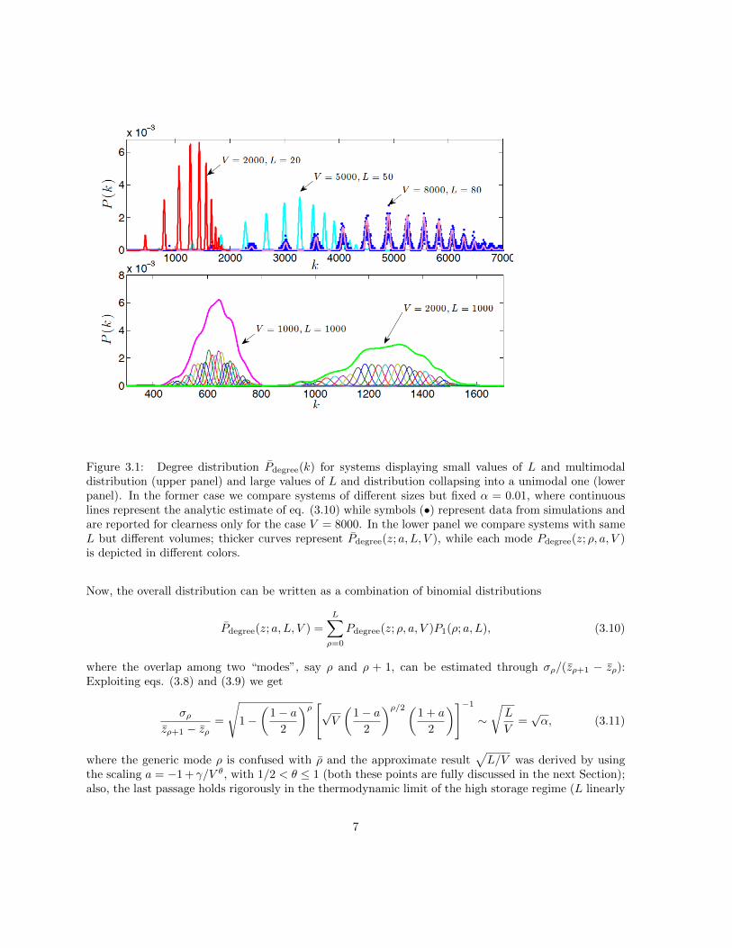
Figure 3.1: Degree distribution Pdegree(k) for systems displaying small values of L and multimodaldistribution (upper panel) and large values of L and distribution collapsing into a unimodal one (lowerpanel). In the former case we compare systems of different sizes but fixed α = 0.01, where continuouslines represent the analytic estimate of eq. (3.10) while symbols (•) represent data from simulations andare reported for clearness only for the case V = 8000. In the lower panel we compare systems with sameL but different volumes; thicker curves represent Pdegree(z; a, L, V ), while each mode Pdegree(z; ρ, a, V )is depicted in different colors.

Now, the overall distribution can be written as a combination of binomial distributions

Pdegree(z; a, L, V ) =

L∑ρ=0

Pdegree(z; ρ, a, V )P1(ρ; a, L), (3.10)

where the overlap among two “modes”, say ρ and ρ + 1, can be estimated through σρ/(zρ+1 − zρ):Exploiting eqs. (3.8) and (3.9) we get

σρzρ+1 − zρ

=

√1−

(1− a

2

)ρ [√V

(1− a

2

)ρ/2(1 + a

2

)]−1

∼√L

V=√α, (3.11)

where the generic mode ρ is confused with ρ and the approximate result√L/V was derived by using

the scaling a = −1 + γ/V θ, with 1/2 < θ ≤ 1 (both these points are fully discussed in the next Section);also, the last passage holds rigorously in the thermodynamic limit of the high storage regime (L linearly

7

diverging with V ). Interestingly, for systems with different scaling regimes among L and V , for instanceL ∝ log V [18, 1], the distribution remains multi-modal because a vanishing overlap occurs among thesingle distributions Pdegree(z; ρ, a, V ): Pdegree(z; a, L, V ) turns out to be an (L + 1)-modal distribution(see Fig. 3.1, upper panel); vice versa, for L ∝ V , the overall distribution gets mono-modal (see Fig. 3.1,lower panel). Briefly, we mention that for θ = 1/2 the ratio in the l.h.s. of eq. (3.11) still converges to afinite value approaching

√α for γ2 � α, while for θ < 1/2 it diverges.

From eq. (3.10), the average degree for a generic node is

z =

V∑z=0

z Pdegree(z; a, L, V ) =

L∑ρ=0

P1(ρ; a;L)zρ = V

1−

[1−

(1 + a

2

)2]L , (3.12)

where

p = 1−

[1−

(1 + a

2

)2]L

(3.13)

is the average link probability for two arbitrary strings ξi and ξj , which can be obtained by averagingover all possible string arrangements, namely, recalling eqs. (3.1) and (3.6),

p =

L∑ρi=0

L∑ρj=0

P1(ρi; a, L)P1(ρj ; a, L)Plink(ρi, ρj ; a, L)

= 1−(

1− a2

)2L L∑ρi=0

L∑ρj=0

(1 + a

1− a

)ρi+ρj (Lρi

)(L− ρiρj

)

= 1−

[1−

(1 + a

2

)2]L

. (3.14)

Of course, eq. (3.14) could be obtained directly by noticing that the probability for the µ-th entries oftwo strings not to yield any contribute is 1 − [(1 + a)/2]2, so that two strings are connected if there isat least one matching.

3.2 Coupling distribution

As explained in Sec. 2, the coupling Jij among nodes i and j is given by the relative number of matchingentries among the corresponding strings ξi and ξj . Eq. (3.4) provides the probability for ξi and ξj toshare a link of magnitude J = k, namely Pcoupling(J ; ρi, ρj , L) = Pmatch(k; ρi, ρj , L). Following the samearguments as in the previous section we get the probability that a link stemming from ξi has magnitudeJ , that is

Pcoupling(J ; ρi, a) =

L∑ρj=0

Pcoupling(J ; ρi, ρj , L)P1(ρj ; a, L) =

(ρiJ

)(1− a

2

)ρi−J (1 + a

2

)J, (3.15)

which is just the probability that J out of ρi non-null entries are properly matched with the genericsecond node.

8

Similarly to Pdegree(z; a, L, V ), the overall coupling distribution can be written as the superposition∑ρ P1(ρ; a, L)Pcoupling(J ; ρ, a), giving rise to a multimodal distribution. Each mode has variance σ2

ρ =

ρ(1− a2)/4 and is peaked at

Jρ = ρ1 + a

2, (3.16)

which represents the average coupling expected for links stemming from a node with ρ non-null entries.Nevertheless, by comparing Jρ+1 − Jρ = (1 + a)/2 and the standard deviation

√ρ(1− a2)/2, we find

that in the limit L = αV and V →∞ the distribution gets mono-modal.

Anyhow, we can still define the average weighted degree wρ expected for a node displaying ρ non-nullentries. Given that for the generic node i, w ≡

∑j Jij , we get

wρ = V Jρ = V ρ1 + a

2. (3.17)

Of course, one expects that the larger the coordination number of a node and the larger its weighteddegree; such a correlation is linear only in the regime of low connectivity. In fact, by merging eq. (3.8)and eq. (3.17), one gets

wρ =

(1 + a

2

)log(1− zρ

V

)log(

1−a2

) V ≈ zρ, (3.18)

where the last expression holds for zρ � V and a� 1.

It is important to stress that (apart pathological cases which will be taken into account in the L → ∞scaling later) the variance of ρ scales as σ2

ρ(a;L) = (1 − a2)L/4 such that, despite the average of ρ is(1 + a)L/2, substituting ρ/L with (1 + a)/2 into eq. (3.18) becomes meaningless in the thermodynamiclimit as the variance of Jρ diverges as

√L ∝

√V : This will affect drastically the thermodynamics

whenever far from the Curie-Weiss limit.

It should be remarked that Jρ represents the average coupling for a link stemming from a node character-ized by a string with ρ non-null entries, where the average includes also non-existing links correspondingto zero coupling. On the other hand, the ratio wρ/zρ directly provides the average magnitude for existingcouplings. Moreover, the average magnitude for a generic link is

J =

L∑ρ=0

P1(ρ; a, L)Jρ =

(1 + a

2

)2

. (3.19)

By comparing eq. (3.16) and eq. (3.19) we notice that the local energetic environment seen by a singlenode, i.e. Jρ, and the overall energetic environment, i.e. J , scale, respectively, linearly and quadraticallywith (1 + a)/2: we will see in the thermodynamic dedicated section that (apart in the Curie-Weiss limitwhere global and local effects merge) despite the self-consistence relation (which is more sensible by

local condition) will be influenced by√J , critical behavior will be found at βc = J−1 coherently with a

manifestation of a collective, global effect.

Anyhow, when V is large and the coupling distribution is narrowly peaked at the mode corresponding toρa,L, the couplings can be rather well approximated by the average value JL(1+a)/2 = [(1 + a)/2]2 = J ,so that the disorder due to the weight distribution may be lost; as we will show this can occur in the

9

regime of high dilution (θ > 1/2). As for the other source of disorder (i.e. topological inhomogeneity),this can also be lost if a is sufficiently larger than −1 as we are going to show.

3.3 Scalings in the thermodynamic limit

In the thermodynamic limit and high-storage regime, L is linearly divergent with V and the averageprobability p for two nodes to be connected (see eq. (3.13)) approaches a discontinuous function assumingvalue 1 when a > −1, and value 0 when a = −1. More precisely, as V → ∞ there exists a vanishinglysmall range of values for a giving rise to a non-trivial graph; such a range is here recognized by thefollowing scaling

a = −1 +γ

V θ, (3.20)

where θ ≥ 0 and γ is a finite parameter.

First of all, we notice that, following eqs. (3.2) and (3.3),

ρ−1+γ/V θ,αV =αγ

2V θ−1(3.21)

σ2−1+γ/V θ,αV =

αγ

2V θ−1

(1− γ

2V θ

)∼ ρ−1+γ/V θ,αV , (3.22)

where the last approximation holds in the thermodynamic limit and it is consistent with the convergenceof the binomial distribution in eq. (3.1) to a Poissonian distribution. For θ ≤ 1, ρ & σ, so that whenreferring to a generic mode ρ, we can take without loss of generality ρ; the case θ > 1 will be neglectedas it corresponds to a disconnected graph.

Indeed, the probability for two arbitrary nodes to be connected gets

p = 1−

[1−

(1 + a

2

)2]L

= 1−[1− γ2

4V 2θ

]αV→

V→∞1− e−γ

2αV 1−2θ/4, (3.23)

so that we can distinguish the following regimes:

• θ < 1/2, p ≈ 1, z ≈ V ⇒ Fully connected (FC) graph

• θ = 1/2, p ∼ 1− e−γ2α/4 ∼ γ2α/4, z = O(V ) ⇒ Linearly diverging connectivityWithin a mean-field description the Erdos-Renyi (ER) random graph with finite probability G(V, p)is recovered.

• 1/2 < θ < 1, p ∼ γ2αV 1−2θ/4, z = O(V 2−2θ) ⇒ Extreme dilution regime (ED)In agreement with [84, 85], limV→∞ z−1 = limV→∞ z/V = 0.

• θ = 1, p ∼ γ2α4V , z = O(V 0) ⇒ Finite connectivity regime

Within a mean-field description γ2α/4 = 1 corresponds to a percolation threshold.

10

Therefore, while θ controls the connectivity regime of the network, γ allows a fine tuning.

As for the average coupling (see eq. (3.19)) and the average weighted degree:

J =γ2

4V 2θ, (3.24)

w = V J =γ2

4V 2θ−1. (3.25)

Now, the average “effective coupling” J , obtained by averaging only on existing links, can be estimatedas

J = J/p =

γ2/(4V 2θ) if θ < 1/2

γ2/[4V 2θ(1− e−γ2α/4)] if θ = 1/21/(αV ) = 1/L if 1/2 < θ ≤ 1

(3.26)

Interestingly, this results suggests that in the thermodynamic limit, for values of a determined byeq. (3.20) with 1/2 < θ ≤ 1, nodes are pairwise either non-connected or connected due to one sin-gle matching among the relevant strings. This can be shown more rigorously by recalling the couplingdistributions Pcoupling(J ; ρi, L) of eq. (3.15): In particular, for θ > 1/2, neglecting higher order cor-rections, for J = 0 the probability is p0 ∼ exp(αγ2V 1−2θ/4) ∼ 1 − γ2α/(4V 2θ−1), for J = 1/L theprobability is p1 ∼ p0γ

2α/(4V 2θ−1) ∼ 1 − p0. For θ = 1/2 this still holds for αγ2/4 � 1, which cor-responds to a relatively high dilution regime, otherwise some degree of disorder is maintained, beingthat pk ∼ (αγ2/4)k/k!. On the other hand, for θ < 1/2, while topological disorder is lost (FC), thedisorder due to the coupling distribution is still present. However, notice that for θ = 0 and γ = 2,Pcoupling(J ; ρi, L) gets peaked at J = L and, again, disorder on couplings is lost so that a pure Curie-Weiss model is recovered.

This means that, for L = αV and V → ∞, we can distinguish three main regions in the parameterspace (θ, α, γ) where the graph presents only topological disorder (θ > 1/2), or only coupling disorder(θ < 1/2), or both (θ = 1/2 ∧ γ2α = O(1)).

In general, we expect that the the critical temperature scales like the connectivity times the averagecoupling and the system can be looked at as a fully connected with average coupling equal to J or as adiluted network with effective coupling J and connectivity given by z; in any case we get β−1

c ∼ J (crf.eq.(4.37)).

3.4 Small-world properties

Small-world networks are endowed, by definition, with high cluster coefficient, i.e. they display sub-networks that are characterized by the presence of connections between almost any two nodes withinthem, and with small diameter, i.e. the mean-shortest path length among two nodes grows logarithmi-cally (or even slower) with V . While the latter requirement is a common property of random graphs[77, 78], the clustering coefficient deserves much more attention also due to the basic role it covers inbiological [86, 87] and social networks [52, 53].

The clustering coefficient measures the likelihood that two neighbors of a node are linked themselves; ahigher clustering coefficient indicates a greater “cliquishness”. Two versions of this measure exist [77, 78]:

11

global and local; as for the latter the coefficient ci associated to a node i tells how well connected theneighborhood of i is. If the neighborhood is fully connected, ci is 1, while a value close to 0 means thatthere are hardly any connections in the neighborhood.

The clustering coefficient of a node is defined as the ratio between the number of connections in theneighborhood of that node and the number of connections if the neighborhood was fully connected. Hereneighborhood of node i means the nodes that are connected to i but does not include i itself. Thereforewe have

ci =2Ei

zi(zi − 1), (3.27)

where Ei is the number of actual links present, while zi(zi−1)/2 is the number of connections for a fullyconnected group of zi nodes. Of course, for the Erdos-Renyi graph where each link is independentlydrawn with a probability p, one has cER = p, regardless of the node considered.

We now estimate the clustering coefficient for the graph G(a, L, V ), focusing the attention on a rangeof a such that the average number of non-null entries per string is small enough for the link probabilityto be strictly lower than 1 so that the topology is non trivial; to fix ideas and recalling last section1/2 ≤ θ ≤ 1. Let us consider a string displaying ρ non-null entries, corresponding to the positionsµ1, µ2, ..., µρ, and z nearest-neighbors; the latter can be divided in ρ groups: strings belonging to thej-th group have ξµj = 1. Neglecting the possibility that a nearest-neighbor can belong to more thanone group contemporary (in the thermodynamic limit this is consistent with Eq. 3.26), we denote withnj the number of nodes belonging to the j-th group, being

∑j nj = z, whose average value is z/ρ

(which, due to the above assumptions is larger than one). Now, nodes belonging to the same groupare all connected with each other as they share at least one common trait, i.e. they form a clique; thecontribute of intra-group links is

Eintra =1

2

ρ∑i=1

ni(ni − 1) =1

2

(ρ∑i=1

n2i − z

)≈ 1

2

[(z

ρ

)2

ρ− z

], (3.28)

while the contribute of inter-group links can be estimated as

Einter ≈ρ∑

i,j=1,i6=j

ninj p ≈(z

ρ

)2(ρ

2

)p, (3.29)

where p is the probability for two nodes linked to i and belonging to different groups to be connected, andthe sum runs over all possible

(ρ2

)couples of groups. Hence, the total number of links among neighbors is

E = Eintra +Einter = {∑ρi=1 ni

∑ρj=1 nj [p+ (1− p)δij ]− z}/2, where δij is the Kronecker delta returning

1 if i = j and zero otherwise; of course, for p = 1 we have E = (z2 − z)/2 and ci = 1.

Now, in the average, the probability p is smaller than p as it represents the probability for two stringsof length L − 1 and displaying an average number of non-null entries equal to ρ − 1 to be connected.However, for ρ and L not too small the two probabilities converge so that by summing the two contributesin eq. (3.28) and (3.29) we get

E ≈ 1

2

[(z

ρ

)2

ρ− z

]+

(z

ρ

)2(ρ

2

)p⇒ c ≈ p+

1

ρ− 1

z − 1> p, (3.30)

12

1 0.9 0.8 0.7 0.6 0.5 0.4 0.3 0.2 0.1 010

20

30

40

50

a

L

0

0.1

0.2

0.3

0.4

0.5

1 0.9 0.8 0.7 0.6 0.5 0.4 0.3 0.2 0.1 010

20

30

40

50

a

L

0

0.2

0.4

0.6

0.8

1

Figure 3.2: Upper panel: average link probability p = z/N ; Lower panel: difference between the averageclustering coefficient for G(V,L, a) and for an analogous ER graph just corresponding to p. Both plotsare presented as function of a and L and refer to a system of V = 2000 nodes.

where in the last inequality we used ρ < z−1. Therefore, it follows straightforward that ci is larger thanthe clustering coefficient expected for an ER graph displaying the same connectivity, that is cER = p.

From previous arguments it is clear that the SW effect gets more evident, with respect to the ERcase taken as reference, when the network is highly diluted. This is confirmed by numerical data:Fig. 3.2 shows in the lower panel the clustering coefficient expected for the analogous ER graph, namelycER = z/V , while in the upper panel it shows the difference between the average local clustering

coefficient c =∑Vi=1 ci/V and cER itself. Of course, when a approaches 1, the graph gets fully connected

and c→ cER → 1.

Finally we mention that when focusing on the low storage regime, a non-trivial distribution for couplingscan give rise to interesting effects. Indeed, weak ties can be shown [88] to work as bridges connectingcommunities strongly linked up, as typical of real networks [52, 89]. Also, as often found in technologicaland biological networks, the graph under study display a “dissortative mixing” [77, 78], that is to say,high-degree vertices prefer to attach to low-degree nodes [88].

13

4 Thermodynamics

So far the emergent network has been exhaustively described by a random, correlated graph whose linksare endowed with weights; we now build up a quantitative thermodynamics on such a structure.

Once the Hamiltonian HV (σ; ξ) is given (eq. 2.2), we can introduce the partition function ZV (β; ξ) as

ZV (β; ξ) =∑σ

e−βHV (σ;ξ), (4.1)

the Boltzmann state ω as

ω(.) =

∑σ .e−βHV (σ;ξ)

ZV (β; ξ),(4.2)

and the related free energy as

A(β, α, a) = limV→∞

1

VE logZV (β; ξ), (4.3)

where E averages over the quenched distributions of the affinities ξ.Once the free energy (or equivalently the pressure) is obtained, remembering that (calling S the entropyand U the internal energy)

A(β, α, a) = −βf(β, α, a) = S(β, α, a)− βU(β, α, a),

the whole macroscopic properties, thermodynamics, can be derived due the Legendre structure of ther-modynamic potentials [67].

4.1 Free energy trough extended double stochastic stability

For the sake of clearness now we expose in complete generality and details the whole plan dealing with ageneric expectation on ξ (i.e. Eξ = (1 + a)/2), then, we will study the L→∞ scaling, in which a musttend to −1 more carefully.With this palimpsest in mind, let us normalize the Hamiltonian (2.2) in a more convenient form for thissection (i.e. dividing by L the Jij , such that the effective coupling is bounded by 1), and let us neglectthe external field h which can be implemented later straightforwardly.

HV (σ; ξ) =1

V L

V∑ij

L∑µ

ξµi ξµj σiσj . (4.4)

As a next step, through the Hubbard-Stratonovick transformation [67, 41], we map the partition functionof our Hamiltonian into a bipartite Erdos-Renyi ferromagnetic random graph [3][47], whose parties arethe former built by the V agents and a new one built of by L Gaussian variables zµ, µ ∈ (1, ..., L):

Z(β; ξ) =∑σ

exp(− βHV (σ; ξ)

)=∑σ

∫ +∞

−∞

L∏µ=1

dµ(zµ) exp(√ β

LV

V∑i

L∑µ

ξi,µσizµ

), (4.5)

14

where with∏Lµ=1 dµ(zµ) we mean the Gaussian measure on the product space of the Gaussian party.

Note that, even when L goes to infinity linearly with V (as in the high storage Hopfield model [11]),due to the normalization encoded into the affinity product of the ξ’s nor the z-diagonal term contributeto the free energy (as happens in the neural network counterpart [23]), neither (but this will be clear atthe end of the section) there is a true dependence by α in the thermodynamics.Furthermore, notice that the graph of the interactions among the two parties is now a simple, and nolonger weighted, Erdos-Renyi [14]: so we started with a complex topology for a single party and we turnedthis problem in solving the thermodynamics for a simpler topology but paying the price of accountingfor another party in interaction. The lack of weight on links will have fundamental importance whendefining the order parameters.Another approach to this is noticing that if we dilute -randomly- directly the Hopfield model (i.e. aschecking for its robustness as already tested by Amit [10]) we push it on an Erdos-Renyi topology, whileif we dilute its entries in pattern definitions (due to the Hebbian kernel) we have to deal with correlateddilution.Consequently (strictly speaking assuming the existence of the V limit) we want to solve for the followingfree energy:

A(β, α, a) = limV→∞

1

VE log

∑σ

∫ +∞

−∞

L∏µ

dµ(zµ) exp(√ β

LV

V∑i

L∑µ

ξi,µσizµ

). (4.6)

To this task we extend the method of the double stochastic stability recently developed in [23] inthe context of neural networks. Namely we introduce independent random fields ηi, i ∈ (1, ..., V ) andχµ, µ ∈ (1, ..., L), (whose probability distribution is the same as for the ξ variables -as in every cavityapproach-), which account for one-body interactions for the agents of the two parties. So our task is tointerpolate among the original system and the one left with only these random perturbations: Let ususe t ∈ [0, 1] for such an interpolation; the trial free energy A(t) is then introduced as follows

A(t) = limV→∞

1

VE log

∑σ

∫ +∞

−∞

L∏µ

dµ(zµ) · (4.7)

· exp(t

√β

LV

V L∑iµ

ξiµσizµ + (1− t)[L∑

lc=1

blc

V∑i

ηiσi +

V∑lb=1

clb

L∑µ

χµzµ

),

where now E = EξEηEχ and blc [with lc ∈ (1, ..., L)], and clb [with lb ∈ (1, ..., V )] are real numbers(possibly functions of β, α) to be set a posteriori.As the theory is no longer Gaussian, we need infinite sets of random fields (mapping the presence ofmulti-overlaps in standard dilution[3][43] and no longer only the first two momenta of the distributions).Of course we recover the proper free energy by evaluating the trial A(t) at t = 1, (A(β, α, a) = A(t = 1)),which we want to obtain by using the fundamental theorem of calculus:

A(1) = A(0) +

∫ 1

0

(∂A(t′)/∂t′

)t′=t

dt. (4.8)

To this task we need two objects: The trial free energy A(t) evaluated at t = 0 and its t-streaming∂tA(t).Before outlining the calculations, some definitions are in order here to lighten the notation: taken g as

15

a generic function of the quenched variables we have

Eηg(η) =

V∑lb=0

P (lb)g(ηlb) =

V∑lb=0

(V

lb

)(1 + a

2

)V−lb (1− a2

)lbg(ηlb), (4.9)

Eχg(χ) =

L∑lc=0

P (lc)g(χlc) =

L∑lc=0

(L

lc

)(1 + a

2

)L−lc (1− a2

)lcg(χlc), (4.10)

Eξg(ξ) =

V∑lb=0

L∑lc=0

(V

lb

)(L

lc

)(1 + a

2

)lb+lc (1− a2

)V+L−lb−lcδlblc=l, (4.11)

where P (lb) is the probability that lb (out of V random fields) are active, i.e. η = 1, so that the number ofspins effectively contributing to the function g is lb; analogously, mutatis mutandis, for P (lc). Moreover,in the last equation we summed over the probability P (l) that in the bipartite graph a number l oflinks out of the possible V × L display a non-null coupling, i.e. ξ 6= 0; interestingly, eq. (4.10) can berewritten in terms of the above mentioned P (lb) and P (lc). In fact, ξi,µ can be looked at as an V × Lmatrix generated by the product of two given vectors like η and χ, namely ξi,µ = ηiχµ, in such a waythat the number of non-null entries in the overall matrix ξ is just given by the number of non-null entriesdisplayed by η times the number of non-null entries displayed by χ. Hence, P (l) is the product of P (lb)and P (lc) conditional to lblc = l.

4.2 The ‘topologically microcanonical” order parameters

Starting with the streaming of eq. (4.7), this operation gives raise to the sum of three terms A+B+ C.The former when deriving the first contribution into the exponential, the last two terms when derivingthe two contributions by all the η and χ.

A = +1

V

√β

LV

V,L∑i,µ

Eξiµω(σizµ) =√αβ

(1 + a

2

) V,L∑lb,lc

P (lb)P (lc)MlbNlc (4.12)

B = −L∑

lc=1

blcV

V∑i

Eηiω(σi) = −L∑

lc=1

blc

(1 + a

2

) V∑lb=0

P (lb)Mlb (4.13)

C = −V∑lb=1

clbN

L∑µ

Eχµω(zµ) = −√α

V∑lb=1

clb

(1 + a

2

) L∑lc=0

P (lc)Nlc , (4.14)

where we introduced the following order parameters

Mlb =1

V

V∑i

ωlb+1(σi), (4.15)

Nlc =1

L

L∑µ

ωlc+1(zµ), (4.16)

and the Boltzmann states ωk are defined by taking into account only k terms among the elements of theparty involved.

16

Of course the Boltzmann states are no longer the ones introduced into the definition (4.2) but theextended ones taking into account the interpolating structure of the cavity fields (which however willrecover the originals of statistical mechanics when evaluated at t = 1).Namely, ωlb+1 has only lb + 1 terms of the type bσ in the Maxwell-Boltzmann exponential, ultimatelyaccounting for the (all equivalent in distribution) lb + 1 values of η = 1, all the others being zero.In the same way ωlc+1 has only lc + 1 terms of the type cz in the Maxwell-Boltzmann exponential,ultimately accounting for the (all equivalent in distribution) lc + 1 values of χ = 1, all the others beingzero.When dealing with ξiµ we can decompose the latter accordingly to what discussed before. By these“partial Boltzmann states” we can define the averages of the order parameters as

〈M〉 =

V−1∑lb

P (lb)Mlb , (4.17)

〈N〉 =

L−1∑lc

P (lc)Nlc . (4.18)

These objects may deserve more explanations because, as a main difference with classical approaches[3][39][43], here replicas and their overlaps are not involved (somehow suggesting the implicit correct-ness of a replica symmetric scenario). Conversely, we do conceptually two (standard) operations whenintroducing our order parameters: at first we average over the (t-extended) Boltzmann measure, thenwe average over the quenched distributions. Let us consider only one party for simplicity: during thefirst operation we do not take the whole party size but only a subsystem, say k spins (whose distributionis symmetric with respect to 0 for both the parties, −1,+1 for the dichotomic, Gaussians for the con-tinuous one). Then, in the second average, for any k from 1 to the volume of the party, we consider allthe possible links among these k nodes in this subgraph. As the links connecting the nodes are alwaysconstant (i.e. equal to one due to the Hubbard-Stratonovich transformation (4.4)) in the intensity, theresulting associated energies are, in distribution and in the thermodynamic limit, all equivalent: We areintroducing a family of microcanonical observables which sum up to a canonical one, in some sense closeto the decomposition introduced in [22].

4.3 The sum rule

Let us now move on and consider the following source S of the fluctuations of the order parameters,where Mlb , Nlc stand for the replica symmetric values4 of the previously introduced order parameters:

S =

(1 + a

2

)√αβ

V−1∑lb

L−1∑lc

P (lb)P (lc)(

(Mlb − Mlb)(Nlc − Nlc))

(4.19)

=

(1 + a

2

)√αβ〈

(M − M

)(N − N

)〉. (4.20)

4strictly speaking there are no replicas here but configurations over different graphs. However the expression RS-approximation, meaning that we assume the probability distribution of the order parameters delta-like over their average(denoted with a bar) is a sort of self-averaging and is an hinge in disordered statistical mechanics such that we allowourselves to retain the same expression with a little abuse of language.

17

We see that with the choice of the parameters blc =√αβNlc and clb =

√β/αMlb , we can write the

t-streaming as

A = S − 1 + a

2

√αβ

V−1∑lb

L−1∑lc

P (lb)P (lc)MlbNlc .

The replica symmetric solution (which is claimed to be the correct expression in diluted ferromagnets)is simply achieved by setting S = 0 and forgetting it from future calculations.We must now evaluate A(0). This term is given by two separate contributions, each for each party.Namely we have

A(0) =1

VE log

∑σ

e∑Llc=1 blc

∑Vi ηiσi +

1

VE log

∫ +∞

−∞

L∏µ=0

dµ(zµ)e∑Vlb=1 clb

∑Lµ χµzµ

= log 2 +

(1 + a

2

) V−1∑lb=0

P (lb)

L−1∑lc=0

P (lc) log cosh(√

αβNlc

)+

(1 + a

2

)2β

2

V−1∑lb

P (lb)M2lb.

Summing A(0) plus the integral of ∂t[A(S = 0)] we finally get

A(t = 1) = log 2 +

(1 + a

2

) L−1∑lc

V−1∑lb

P (lc)P (lb) log cosh(√

αβNlc

)(4.21)

+β

2

(1 + a

2

)2 L−1∑lb

P (lb)M2lb− 1 + a

2

√αβ

V−1∑lb

L−1∑lc

P (lb)P (lc)MlbNlc . (4.22)

It is possible to show that (as each bipartite ferromagnetic model [23][48]) the free energy obeys amin-max principle by which, extremizing the free energy with respect to the order parameters we canexpress 〈N〉 trough 〈M〉: The trial replica symmetric solution, expressed trough 〈M〉, 〈N〉 is (at fixed〈N〉) convex in 〈M〉. This defines uniquely a value 〈M(N)〉 where we get the max. Further, 〈M(N)〉 isincreasing and convex in 〈N2〉 such that the following extremization is a well defined procedure.

∑k

P (k)∂A

∂Mk= 0→

∑lc

P (lc)Nlc =∑k

P (k)1 + a

2

√β

αMk, (4.23)

∑k

P (k)∂A

∂Nlk= 0→

∑lb

P (lb)Mlb =∑k

P (k) tanh(√

αβNk

). (4.24)

Due to the mean field nature of the model, as we can express Nk trough the average of the Mk, we canwrite the free energy of our network trough the series of Mlb alone [as expected as we started by eq.(2.2)]

A(β, a) = log 2 + (1 + a

2) log cosh

(tanh−1[

∑lb

P (lb)Mlb ])

(4.25)

+β

2(1 + a

2)2∑lb

P (lb)M2lb− (

1 + a

2)∑lb

P (lb)Mlb tanh−1(∑

l′b

P (lb′)Ml′b

).

As anticipated there is no true dependence by α. Note that without normalizing the scalar productamong the bit strings we should rescale β accordingly with α, as in the L → ∞ limit we would get an

18

infinite coupling (which is physically meaningless).Before exploring further properties of these networks, we should recover the well known limit of Curie-Weiss a = +1 and isolate spin system a = −1.Let us work out for the sake of clearness the self-consistency in a purely Curie-Weiss style by extremizing,with respect to 〈M, 〉 eq. (4.25):

∂〈M〉A(β) = (1 + a

2)( 〈M〉

1− 〈M〉2+ β(

1 + a

2)〈M〉

)− (

1 + a

2)( 〈M〉

1− 〈M〉2+ tanh−1〈M〉

)= 0

⇒ 〈M〉 = tanh(β(1 + a

2)〈M〉)⇒ tanh−1〈M〉 = β(

1 + a

2)〈M〉, (4.26)

such that the to get the classical magnetization in our model we have to sum overall the contributinggraphs, namely 〈MCW 〉 = 〈M〉 =

∑lbP (lb)Mlb , and we immediately recover

a→ −1 ⇒ A(β, a = −1) = log 2, (4.27)

a = +1 ⇒ A(β, a = +1) = log 2 + log cosh(β〈M〉)− β

2〈M2〉, (4.28)

which are the correct limits (note that in eq. (4.27) J = 0, while in eq. (4.28) J = 1).Furthermore, we stress that in our “topological microcanonical” decomposition of our order parameters,when summing over all the possible subgraphs to obtain the CW magnetization, these are all nullapart the only surviving of the fully connected network, so the distribution of the order parametersbecomes trivially ∝ δ(M −MCW ), namely, only one order parameter survives, the classical Curie-Weissmagnetization.

4.4 Critical line trough fluctuation theory

Developing a fluctuation theory of the order parameters allows to determine where critical behaviorarises and, ultimately, the existence of a phase transition5.To this task we have at first to work out the general streaming equation with respect to the t-flux.Given a generic observable O defined on the space of the σ, z variables, it is immediate to check that thefollowing relation holds (we set α = 1 for the sake of simplicity as it never appears in the calculations(as can be easily checked by substituting 〈N〉 with 〈M〉 trough eq. (4.23) which changes the prefactorfrom ( 1+a

2 )√αβ → ( 1+a

2 )2β and express the fluctuations only via the real variables σ 6):

∂〈O〉∂t

=1 + a

2

√β[(〈OMN〉 − 〈O〉〈MN〉)− N(〈OM〉 − 〈O〉〈M〉)− M(〈ON〉 − 〈O〉〈N〉)

], (4.29)

where we defined the centered and rescaled order parameters:

〈M〉 =√V∑lb

P (lb)(Mlb − Mlb) =√V 〈M − M〉, (4.30)

〈N〉 =√L∑lc

P (lc)(N − N) =√L〈N − N〉. (4.31)

5Strictly speaking this approach holds only for second order phase transition, which indeed is the one expected inimitative models, even in presence of dilution [3].

6Another simple argument to understand the useless of α is a comparison among neural networks: in that context, αrules -in the thermodynamic limit- the velocity by which we add stored memories into the network with respect to thevelocity by which we add neurons. If the former are faster than a critical value, by a TLC argument they sum up to aGaussian before the infinite volume limit has been achieved and the Hopfield model turns into an SK[23]. Here there is nodanger in this as we have only positive -normalized- interactions.

19

Now we focus on their squares: We want to obtain the behavior of 〈M2〉t=1, 〈MN〉t=1, 〈N 2〉t=1, so tosee where their divergencies (onsetting the phase transition) are located.By defining the dot operator as

〈O〉 = (1 + a

2)√β∂t〈O〉 (4.32)

we can write

˙〈M2〉 =[〈M3N〉 − 〈M2〉〈MN〉 − N〈M3〉+ N〈M2〉〈M〉 − M〈M2N〉+ M〈M2N〉

],

˙〈MN〉 =[〈M2N 2〉 − 〈MN〉〈MN〉 − N(〈M2N〉 − 〈MN〉〈M〉)− M(〈MN 2〉 − 〈MN〉〈N〉)

],

˙〈N 2〉 =[〈N 3M〉− 〈N 2〉〈MN〉 − N〈N 2M〉+ N〈N 2〉〈M〉 − M〈N 3〉+ M〈N 2〉〈N〉

].

Now, for the sake of simplicity, let us introduce alternative labels for the fundamental observables. Wedefine A(t) = 〈M2〉t, D(t) = 〈MN〉t and G(t) = 〈N 2〉t and let us work out their t = 0 value, whichis straightforward as at t = 0 everything is factorized (alternatively these can be seen as high noiseexpectations):

A(t = 0) = 1, D(t = 0) = 0, G(t = 0) =(

1 + (1 + a

2)2 β

α〈M2〉

)− 〈N2〉 = 1

where we used the self-consistence relation (4.23) and assumed that at least where everything is com-pletely factorized the replica solution is the true solution7. Following the technique introduced in [51],starting from the high temperature and, under the Gaussian ansatz for critical fluctuations, we want totake into account correlations among the order parameters. Within this approach, using Wick theoremto split the four observable averages in series of couples, the (formal) dynamical system reduces to

A(t) = 2A(t)D(t), (4.33)

D(t) = A(t)G(t) +D2(t), (4.34)

G(t) = 2G(t)D(t). (4.35)

We must now solve for A(t), D(t), G(t) and evaluate these expression at t = 1+a2

√β accordingly to the

definition of the dot operator in eq.(4.32). Notice at first that

∂t logA =A

A= 2D =

G

G= ∂t logG.

This means ∂t(A/G) = 0 and as A(0)/G(0) = 1 we already know that A(t) = G(t): the fluctuations ofthe two order parameters behave in the same way, not surprisingly, as already pointed out their mutualinterdependence several times.We are left with

D(t) = G2(t) +D2(t), (4.36)

G(t) = 2G(t)D(t). (4.37)

By defining Y = D + G we immediately get, summing the two equations above: Y = Y 2 by which weget Y (t) = Y (0)/(1− tY (0)). As Y (0) = 1 we obtain that

D(t = (1 + a

2)√β) +G(t = (

1 + a

2)√β) =

1

1− ( 1+a2 )√β,

7Any debate concerning RSB on diluted ferromagnets is however ruled out here as we are approaching the critical linefrom above.

20

so there is a regular behavior up to βc = 1/( 1+a2 )2.

We must now solve separately for D and G: this is straightforward by introducing the function Z = G−1

and checking that Z obeys−Z − 2Y Z + 2 = 0,

which, once solved with standard techniques (as Y is known) gives G(t) = [2(1 − t)]−1 and ultimately,simply by noticing the divergencies of A(t = (1 + a)

√β/2), D(t = (1 + a)

√β/2), G(t = (1 + a)

√β/2),

we get the critical line for both the squared order parameters and their relative correlation: All thesefunctions do diverge on the line

βc =1

( 1+a2 )2

=1

J, (4.38)

defining a phase transition according with intuition.

4.5 L→∞ scaling in the thermodynamic limit

As we understood in Section (3.3), in the V → ∞ and L → ∞ limits we need to tune the limit ofa → −1 carefully to recover the various interesting topologies and to avoid the trivial limits of fullyconnected/disconnected graph.

In particular, a must approach −1 as a = −1 + γ/V θ. To tackle this scaling it is convenient to usedirectly γ, θ as tunable parameter and rewrite the Hamiltonian in the following forms8

HV (σ; ξ) =1

2αV 2(1−θ)

V∑ij

L∑µ

ξµi ξµj σiσj ⇒ HV,L(σ, z; ξ) =

√β/α

V 1−θ

∑i,µ

ξi,µσizµ, (4.39)

where the difference among the two expression H, H is due to the Hubbard-Stratonovick transformationapplied to the coupled partition functions, as performed early trough eq.(4.4).Our free energy reads off now as

A(α, β, γ, θ) = limV→∞

1

VE log

∑σ

∫ L∏µ

dµ(zµ) exp(

√β/α

V (1−θ) )∑i,µ

ξiµσizµ, (4.40)

where α accounts for the different ratio among the two parties, β the noise into the network, θ selectsthe graph (see Sec.(3.3)) and γ is the fine tuning inside the chosen topology.The interpolating scheme remains the same: we introduce the right amount of random fields and uset ∈ (0, 1) to define

A(t) =1

NE log

∑σ

∫dµ(zµ) exp[tHV,L(σ, z; ξ) + (1− t)(

∑i

aηiσi +∑µ

bηµzµ)]. (4.41)

By performing the t-streaming easily we get

∂tA(t) =

√βγ

2〈(M − M)(N − N)〉+

√βγ

2MN , (4.42)

8As we are going to see soon it is not possible to normalize the Hamiltonian -both the coupling strength and the volumeextensiveness- for all the possible graphs in only one expression. We choose to normalize so to tackle immediately thebetter known limits, however apparent divergencies in the couplings develop and can be standardly avoided by properlyrescaling the temperature corresponding to the amount of nearest neighbors, as in more classical approaches.

21

such that the replica symmetric sum rule gets

A(1) = A(0)−√βγ

2MN , (4.43)

and the replica symmetric free energy reads off as

A(β, γ, θ) = log 2 +γ

2V θlog cosh(

√βNV θ) +

βγ2

8M2 −

√βγ

2MN . (4.44)

Let us now investigate some limits of this expression and its self-consistency. Note that by extremizingwith respect to the order parameters we can skip N trough M as

〈N〉 =

√βγ

2〈M〉. (4.45)

4.5.1 θ = 0 case: Fully connected, weighted and Curie-Weiss scenario

The case θ = 0 reduces to a fully connected graph, and in particular in the upper bound for γ (i.e.γ = 2) its topology recovers the unweighed CW model (see sec. 3.3). We should recover here even theCW thermodynamics.

A(β, γ, θ = 0) = log 2 +γ

2log cosh(β

γ

2〈M〉)− βγ2

8〈M〉2, (4.46)

and its self-consistency relation reduces to

〈M〉 = tanh(βγ

2〈M)〉.

This holds generally for the weighted graph; in particular when γ = 2 ⇒ J = 1 and the graph getsun-weighted (still fully connected), we get the standard Curie-Weiss limit once more:

A(β, γ = 2, θ = 0) = log 2 + log cosh(β〈M〉)− β2〈M〉2, (4.47)

〈M〉 = tanh(β〈M〉). (4.48)

4.5.2 θ = 1/2: Standard dilution and Erdos-Renyi scenario

With a scheme perfectly coherent with the previous one we can write down free energy and its coupledself-consistency as

A(β, γ, θ = 1/2) = limV→∞

(log 2 +

γ

2√V

log cosh(βγ

2

√V 〈M〉)− βγ2

8〈M〉2

), (4.49)

〈M〉 = limV→∞

tanh(βγ

2

√V 〈M〉). (4.50)

Let us stress that, as√J = γ

2√V

, the argument of the logarithm of the hyperbolic cosine scales as√JV 〈M〉: This is coherent with the lack of a proper normalization into the Hamiltonian (4.39) because

22

for θ = 1/2 the latter is still divided by V which should not appear. To avoid the lack of a universalnormalization, we need to renormalize the local average coupling by a factor V so that we get the correctbehavior, namely we write explicitly the free energy putting in evidence that p ∼ 1− exp(−αγ2/4):

A(β, γ, θ = 1/2) = log 2 +√J log cosh(

β√J

p〈M〉)− βJ

2p〈M〉2, (4.51)

such that, being β = βpV [3], we can easily recover the trivial limits of the CW case when p → 1 (andchoerently J → 1, β → β) and of the fully disconnected network p→ 0⇒ A(β, γ → 0, θ = 1/2) = log 2as p is superlinear in γ.

4.5.3 θ = 1: Extreme diluted regime

With a scheme perfectly coherent with the previous one we can write down free energy and its coupledself-consistency as

A(β, γ, θ = 1) = limV→∞

(log 2 +

γ

2Vlog cosh(

βγ

2V 〈M〉)− βγ2

8〈M〉2

), (4.52)

〈M〉 = limV→∞

tanh(βγ

2V 〈M〉). (4.53)

Of course here, with respect to the previous case, we get even stronger divergencies. Now we need torenormalize the local average coupling by a factor V 2.

4.6 Numerics: Probability distribution

As the critical line is obtained, in the fluctuation theory, through the Gaussian ansatz, we double checkour finding via numerical simulations.

First of all, we notice that since the interaction matrix Jij is symmetric (Jij = Jji), detailed balanceholds and it is well known [69, 4] how to introduce a Markov process for the dynamical evolution ruledby Hamiltonian (2.2) and obtain the transition rates for stationarity: Montecarlo sampling is thenmeaningful for equilibrium investigation.

The order parameter distribution function has been proved to be a powerful tool for studying the criticalline in different kinds of systems; in particular, for magnetic systems the order parameter can be chosenas the magnetization per spin which, in finite-size systems, is a fluctuating quantity characterized bya probability distribution P (m) [27]. In Ising-like models undergoing a second-order phase transitionit is known that at temperatures lower than the critical temperature β−1

c , the distribution P (m) has adouble peak, centered at the spontaneous magnetization +m and −m. At temperatures greater thanβ−1c , P (m) has a single peak at zero magnetization, and exactly at β−1

c a double peak shape is observed.

In Fig. 4.1 we plotted numerical data for the probability distribution, obtained by means of Monte Carlosimulations, where P (m) corresponds to the fraction of the total number of realizations in which the

23

−1 −0.5 0 0.5 10

0.05

0.1

0.15

0.2

0.25

0.3

0.35

m

P(m

)

0.98 0.9805 0.981 0.9815 0.9820

0.05

0.1

0.15

0.2

0.25

0.3

m

P(m

)

V = 120V = 500V = 1000

Figure 4.1: Probability distribution for the order parameter P (m). Main figure: system of size N = 1000at a temperature T = 0.5Tc; Inset: comparison between systems of size N = 120, N = 500 and N = 1000,as shown by the legend, set at a temperature T = 0.9Tc.

system magnetization is m. In the main figure we show the distribution for a system with V = 1000 set ata temperature β−1 = 1.1β−1

c , while in the inset we compare system of different sizes set at a temperatureβ−1 = 2β−1

c . Notice that, for such small temperatures, as the size in increased the distribution is moreand more peaked, while the probability to have zero magnetization is vanishing; this corroborates thereplica-symmetric ansatz.

5 Conclusion

In this paper we pioneered an alternative way for obtaining complex topologies. Interestingly from ourapproach small world features are emergent properties and no longer imposed a-priori, furthermore thecore-theory descents from a simple shift −1→ 0 in the definition domain of the patterns of an Hopfieldmodel and is able to recover all the best known complex topologies.From a graph theory perspective we introduced a model which, given a set of V nodes, each correspondingto a set of L attributes encoded by a binary string ξ, defines an interaction coupling Jij = (ξi ·ξj) for anycouple of nodes (i, j). The resulting system can be envisaged by means of a weighted graph displayingnon trivial correlations among links. In particular, when attributes are extracted according to a discreteuniform distribution, i.e. P (ξµi ) = (1+a)/2 for any i ∈ [1, V ] and µ ∈ [1, L], being a a tunable parameter,we get that when a is sufficiently small the resulting network exhibits a small-world nature, namely alarge clustering coefficient; As a is spanned, the network behaves as an isolate spin system, an extremedilute network, a linearly diverging connectivity network a weighted fully connected and an un-weighted

24

fully connected network, respectively. Moreover, nodes are topologically distinguishable according tothe concentration ρ of non-null entries present in their corresponding binary strings: interestingly, if thescaling among L and V is sub-linear (i.e. P ∝ lnV or even slower as in low storage networks [1, 18]) thedegree distribution turns out to be multi-modal, each mode pertaining to a different value of ρ. Instead,whenever the scaling is (at least) linear -L ∝ V -, the distribution gets mono-modal. At least numeri-cally, at finite V,L, when looking at the distribution of weights, one finds that weak-ties work as bridge,in full agreement with Granovetter theory: indeed, one can detect small highly-connected clusters or”communities” made up of nodes with similar attributes and links connecting different communities arefound to correspond a small coupling.Then, as diluted models are of primary interest in disordered statistical mechanics, by assuming self-averaging of the order parameters, we solved the thermodynamic of the model: this required a newtechnique (a generalization to infinitely random fields of the double stochastic stability) which is ofcomplete generality as well and paves another way for approaching dilution in complex systems.Furthermore, within this framework, replicas are not necessary and instead of averaging over these copiesof the system (and dealing with the corresponding overlap) we can obtain observables as magnetizationaverages over local subgraphs, implicitly accounting for a replica symmetric behavior (which is indeedassumed trough the study).An interesting finding, on which both the investigations converge (graph theory and statistical mechan-ics), is a peculiar non-mean field effect in the overall fields felt by the spins: from eq. (3.17) we seethat the field insisting on a spin scales as

√J while the averaged field on the network scales as J -see

eq. (3.20)- (which is the canonical mean field expectation). Furthermore, looking at eq. (4.25) wesee that in the hyperbolic tangent encoding the response of the spin to the fields, the contribution ofthe other spins is not weighted by J but by

√J . As in the thermodynamics the coupling strength has

been normalized, J < 1 →√J > J : in complex thermodynamics there is a super-linearity among the

interactions: despite this does not affect the critical behavior which is a global feature of the systemand consequently is found to scale with J (see eq. (4.37)), this may substantially change all the otherspeculations based on intuition.Of course, in the Curie-Weiss limit this effect disappear as global and local environments do coincide(i.e. J = 1).It is worth stressing that (microscopic) correlation among bit-strings is directly related to macroscopicbehavior (e.g. critical line), providing a new intriguing mechanics to study the former via investigationson the latter (e.g. in social networks, gene regulatory networks, or immune networks).Next step in the research now should be double directed: from one side, a clear statistical mechanicsof scale free networks may stem from our approach. From the other side, applications of this theory toreal systems (first at all a clear investigation on dynamical retrieval properties), both in biology and insociology, should be a primary challenge as well.

Acknowledgments

Francesco Guerra as usual is acknowledged for priceless scientific and human interchange.This work is supported by the FIRB grant: RBFR08EKEVAB is grateful even to the Smart-Life Grant for partial support.INFN and GNFM are acknowledged too for their partial support.

25

References

[1] E. Agliari, A. Barra, Statistical mechanics of idiotypic immune networks, submitted to J. Theor. Bio.(2010).

[2] E. Agliari, R. Burioni, Random Walk on Deterministic Scale-Free networks, Phys. Rev. E, 80, 031125(2009).

[3] E. Agliari, A. Barra, F. Camboni, Criticality in diluted ferromagnets, J. Stat. Mech. P10003, (2008).

[4] E. Agliari, A. Barra, R. Burioni, P. Contucci, New perspectives in the equilibrium statistical mechanicsapproach to social and economic sciences, Mathematical modeling of collective behavior in socio-economic and life sciences, Birkhauser Editor (2010).

[5] E. Agliari, R. Burioni, D. Cassi, F.M. Neri Autocatalytic Reactions on low-dimensional structures,Thoer. Chem. Acc., 118, 855 (2007).

[6] E. Agliari, A. Blumen, O. Mulken, Dynamics of Continuous-time quantum walks in restricted ge-ometries, J. Phys. A, 41, 445301 (2008).

[7] E. Agliari, M. Casartelli, A. Vezzani, Energy transport in an Ising disordered model, J. Stat. Mech.,07041 (2009).

[8] E. Agliari, M. Casartelli, E. Vivo, Metric characterization of cluster dynamics on the Sierpinskigasket, submitted.

[9] D. ben-Avraham, S. Havlin, Diffusion and Reactions in Fractals and Disordered Systems, CambridgeUniversity Press, (2000).

[10] D.J. Amit, Modeling brain function: The world of attractor neural network Cambridge UniverisityPress, (1992)

[11] D.J. Amit, H. Gutfreund, H. Sompolinsky, Storing infinite numbers of patterns in a spin glass modelof neural networks, Phys. Rev. Lett. 55, (1985).

[12] D.J. Amit, H. Gutfreund, H. Sompolinsky, Information storage in neural networks with low levelsof activiy, Phys. Rev. A 35, (1987).

[13] D.J. Amit, H. Gutfreund, H. Sompolinsky, Information storage in neural networks with low levelsof activiy, Phys. Rev. A 35, (1987).

[14] R. Albert, A. L. Barabasi Statistical mechanics of complex networks, Reviews of Modern Physics74, 47-97 (2002).

[15] A. L. Barabasi, Z. N. Oltvai, Network biology: understanding the cell’s functional organization, Rev.Nature Genetics 5, 101-116, (2004).

[16] A. Barra, The mean field Ising model trhought interpolating techniques, J. Stat. Phys. 132, N.5,787-809, (2008).

[17] A. Barra, Irreducible free energy expansion and overlap locking in mean field spin glasses, J. Stat.Phys. 123, N.3, 601-614, (2006).

26

[18] A. Barra, E. Agliari, Autopoietic immune networks from a statistical mechanics perspective, J. Stat.Mech. P07004, (2010).

[19] A. Barra, E. Agliari, Stochastic dynamics for idiotypic immune networks, submitted to Physica A(2010).

[20] A. Barra, F. Camboni, P. Contucci, Dilution robustness for mean field ferromagnets, J. Stat. Mech.P03028, (2009).

[21] A. Barra, P. Contucci, Toward a quantitative approach to migrants integration, Europhys. Lett. 89,68001− 68007, (2010).

[22] A. Barra, F. Guerra, About the ergodicity in Hopfield analogical neural network, J. Math. Phys. 49,125217, (2008).

[23] A. Barra, F. Guerra, G. Genovese, The replica symmetric behavior of the analogical neural network,J. Stat. Phys. 140, N.4, 784− 796, (2010).

[24] A. Barrat, M. Weigt, On the properties of small-world network models, Europ. Phys. J. B 13, 547,(2000).

[25] A. Barrat, M. Barthelemy, A. Vespignani, Dynamical processes in complex networks, CambridgeUniversity Press (2008).

[26] D. ben-Avraham, S. Havlin, Diffusion and Reactions in Fractals and Disordered Systems, CambridgeUniversity Press (200).

[27] K. Binder, D. P. Landau, Guide To Monte Carlo Simulations In Statistical Physics, CambridgeUniversity Press (2009).

[28] C. C. F. Blake, Do genes in pieces imply proteins in pieces? Nature 273, 267 (1978).

[29] B. Bollobas, Random graphs, Cambridge Stud. Advanc. Math., Cambr. Univ. Press. (1985).

[30] J.P. Bouchaud, M. Potters, Theory of financial risks: from statistical physics to risk managemenent,Oxford University Press, (2004).

[31] R. Burioni, D. Cassi, Energy transport in an Ising disordered model, J. Phys. A, 38, R45 (2005).

[32] W. Brock, S. Durlauf, Discrete choices with social interactions, Rev. Econ. St. 68, (2001).

[33] M. Buchanan, Nexus: Small Worlds and the Groundbreaking Theory of Networks. Norton, W. W.Company, Inc. (2003).

[34] M. Buchanan,G. Caldarelli , P. De Los Rios, F. Rao and M. Vendruscolo (eds), M. Modelling cellbiology with networks, Cambridge Univ. Press (2010).

[35] F.M. Burnet, The clonal selection theory of acquired immunity, Cambridge University Press, (1959).

[36] D. Callaway, M.E.J. Newman, S.H. Strogats, D.J. Watts, Network robustness and fragility: Perco-lation on random graphs, Phys. Rev. Lett. 85, 5468 (2000).

[37] A.C.C. Coolen, R. Kuehn, P. Sollich, Theory of Neural Information Processing Systems, OxfordUniv. Press, (2005).

27

[38] A.C.C. Coolen, S. Rabello, Generating functional analysis of complex formation and dissociationin large protein interaction networks, Proc. IW-SMI-2009, Kyoto, J. Phys. Conference Series, (2009).

[39] A. Dembo, A. Montanari. Gibbs Measures and Phase Transitions on Sparse Random Graphs, coursetaught at the 2008 Brazilian School of Probability (2008).

[40] S.N. Durlauf, How can statistical mechanics contribute to social science?, Proc. Natl. Ac. Sc. 96,(1999).

[41] R.S. Ellis, Large deviations and statistical mechanics, Springer, New York (1985).

[42] C. Francke, R.J. Siezen, B. Teusink, Reconstructing the metabolic network of a bacterium from itsgenome, Trends in Microbiol. 13, 550− 558, (2005).

[43] L. De Sanctis, F. Guerra, Mean field dilute ferromagnet I. High temperature and zero temperaturebehavior, J. Stat. Phys. 132, (2008).

[44] M. Galiceanu, A. Blumen, Spectra of Husimi cacti: Exact results and applications, J. Chem. Phys.,127, 134904 (2007).

[45] I. Gallo, A. Barra, P. Contucci, Parameter Evaluation of a Simple Mean-Field Model of SocialInteraction, Math. Meth. & Models in Applied Sciences 19, 1427− 1439, (2008).

[46] A.C. Gavin et al., Functional organization of the yeast proteome by systematic analysis of proteincomplexes, Nature 415, 141− 147, (2002).

[47] G. Genovese, A. Barra, A mechanical approach to mean field spin models, J. Math. Phys. 50, 053303,(2009).

[48] G. Genovese, A. Barra, A certain class of Curie-Weiss models, arXiv:0906.4673, (2009).

[49] L.H. Greene, V.A.Higman, Uncovering network system within protein structures, J. Molec. Bio.334, (2003).

[50] F. Guerra, Broken Replica Symmetry Bounds in the Mean Field Spin Glass Model, Comm. Math.Phys. 233, 1-12, (2003).

[51] F. Guerra, Sum rules for the free energy in the mean field spin glass model, in Mathematical Physicsin Mathematics and Physics: Quantum and Operator Algebraic Aspects, Fields Institute Communica-tions 30, Amer. Math. Soc. (2001).

[52] M.S. Granovetter, The Strength of Weak Ties, Amer. J. of Sociology 78, 1360− 80, (1973).

[53] M.S. Granovetter, The Strength of the Weak Tie: Revisited, Sociol. Theory 1, 201− 33, (1983).

[54] E.L. Berlow, Strong effects of weak interactions in ecological communities, Letters to Nature 398,330− 334, (1999).

[55] D.O. Hebb, Organization of Behaviour, Wiley, New York, (1949).

[56] J.J. Hopfield, Neural networks and physical systems with emergent collective computational abilities,P.N.A.S. 79, (1982).

[57] E. Jantsch, The Self-Organizing Universe: Scientific and Human Implications of the EmergingParadigm of Evolution, Sys. Sc. World Order Libr. (1990).

28

[58] N.K. Jerne, Toward a network theory of the immune system, Ann. Immun. 125, (1974).

[59] C. Martelli, A. De Martino, E. Marinari, M. Marsili, I. Perez-Castillo, Identifying essential genesin E. coli from a metabolic optimization principle, Proc. Natl. Acad. Sc. 106 2607, (2009).

[60] D. McFadden, Economic choices, American Econ. Rev. 91, 351− 378, (2001).

[61] D. Medini, A. Covacci, and C. Donati, Protein Homology Network Families Reveal step-wise diver-sification, PLoS 2, Comp. Bio., 12, (2006).

[62] M. Mezard, G. Parisi and M. A. Virasoro, Spin glass theory and beyond, World Scientific, Singapore(1987).

[63] S. Milgram, The Small World Problem, Psych. Today 2, 60− 67, (1967).

[64] J. M. Montoya, R. V. Sole’, Small World Patterns in Food Webs, J. Theor. Biol. 214, 3, (2002).

[65] T. Nikoletopoulos, A.C.C. Coolen, I. Perez-Castillo, N.S. Skantzos, J.P.L. Hatchett, B. Wemmen-hove, Replicated Transfer Matrix Analysis of Ising Spin Models on ‘Small World’ Lattices, J. Phys. A37, (2004).

[66] G. Parisi, A simple model for the immune network, P.N.A.S. 87, (1990).

[67] G. Parisi, Statistical field theory, Frontiers in physics, (1998).

[68] L. Peliti, Introduction to the statistical theory of Darwinian evolution, Lectures at the SummerCollege on Frustrated System, Trieste, August (1997).

[69] I. Perez-Castillo, B. Wemmenhove, J.P.L. Hatchett, A.C.C. Coolen, N.S. Skantzos, T. Nikoletopou-los, Analytic Solution of Attractor Neural Networks on Scale-free Graphs, J. Phys. A 37, (2004).

[70] S. Rabello, A.C.C. Coolen, C.J. Perez-Vicente and F. Fraternali, A solvable model of the genesisof amino-acid sequences via coupled dynamics of folding and slow genetic variation, J. Phys. A 41,285004, (2008).

[71] D.J. Watts, S.H. Strogatz, Collective dynamics of small world networks, Nature 393, (1998).

[72] D.J. Watts. An Experimental Study of Search in Global Social Networks, Science, (2003).

[73] Z. Furedi and J. Komlos, The eigenvalues of random symmetric matrices, Combinatorica 1 (1981),no. 3, 233-241

[74] D. Achlioptas, R. M. D’Souza, J. Spenceer, Explosive Percolation in Random Networks, Science,323, 1453 (2009)

[75] A.A. Moreira, E.A. Oliveira, S.D.S. Reis, H.J. Herrmann, J.S. Andrade Jr., A Hamiltonian approachfor explosive percolation archivio

[76] H.D. Rozenfeld, L.K. Gallos, H.A. Makse, Explosive percolation in the Human Protein HomologyNetwork archivio

[77] M.E.J. Newman, The structure and function of complex networks, SIAM Review, 45, 167-256 (2003),and references therein

29

[78] R. Albert and A.-L. Barabasi, Statistical mechanics of Complex Networks, Rev. Mod. Phys. 74,47-98 (2002), and references therein

[79] M. Molloy and B. Reed, The size of the giant component of a random graph with a given degreesequence, Combinatorics, Probability and Computing 7, 295-305 (1998)

[80] H. Jeong, S.P. Mason, Z.N. Oltvai and A.-L. Barabasi ?, Nature 411, 41 (2001)

[81] M.E.J. Newman, Assortativity Mixing in Networks, Phys. Rev. Lett., 89, 208701 (2002)

[82] G.R. Grimmett, Percolation, Spinger-Verlag, Berlin 1999.

[83] B. Bollobas, O. Riordan Percolation, Cambridge University Press, Cambridge 2006.

[84] Watkin T L H and Sherrington D 1991, Europhys. Lett. 14, 791

[85] B. Wemmenhove, N. S. Skantzos, A. C. C. Coolen, 2004 J. Phys. A: Math. Gen. 37, 7653

[86] Said M R, Begley T J, Oppenheim A V, Lauffenberger D A and Samson L D 2004, Proc. Nat. Am.Soc. 101, 18006

[87] Uetz P, Dong Y-A, Zeretzke C, Atzler C, Baiker A, Berger B, Rajagopala S V, Roupelieva M, RoseD, Fossum E and Haas J, 2006 Science 311, 239

[88] E. Agliari, A. Barra, forthcoming.

[89] Breskin I, Soriano J, Moses E and Tlusty T, 2006, Phys. Rev. Lett. 97, 188102

30