DISTRIBUTED DATABASES

JAN 2014 Slide 1DISTRIBUTED DBMS

DISTRIBUTED DATABASES

E0 261

Jayant Haritsa

Computer Science and Automation

Indian Institute of Science


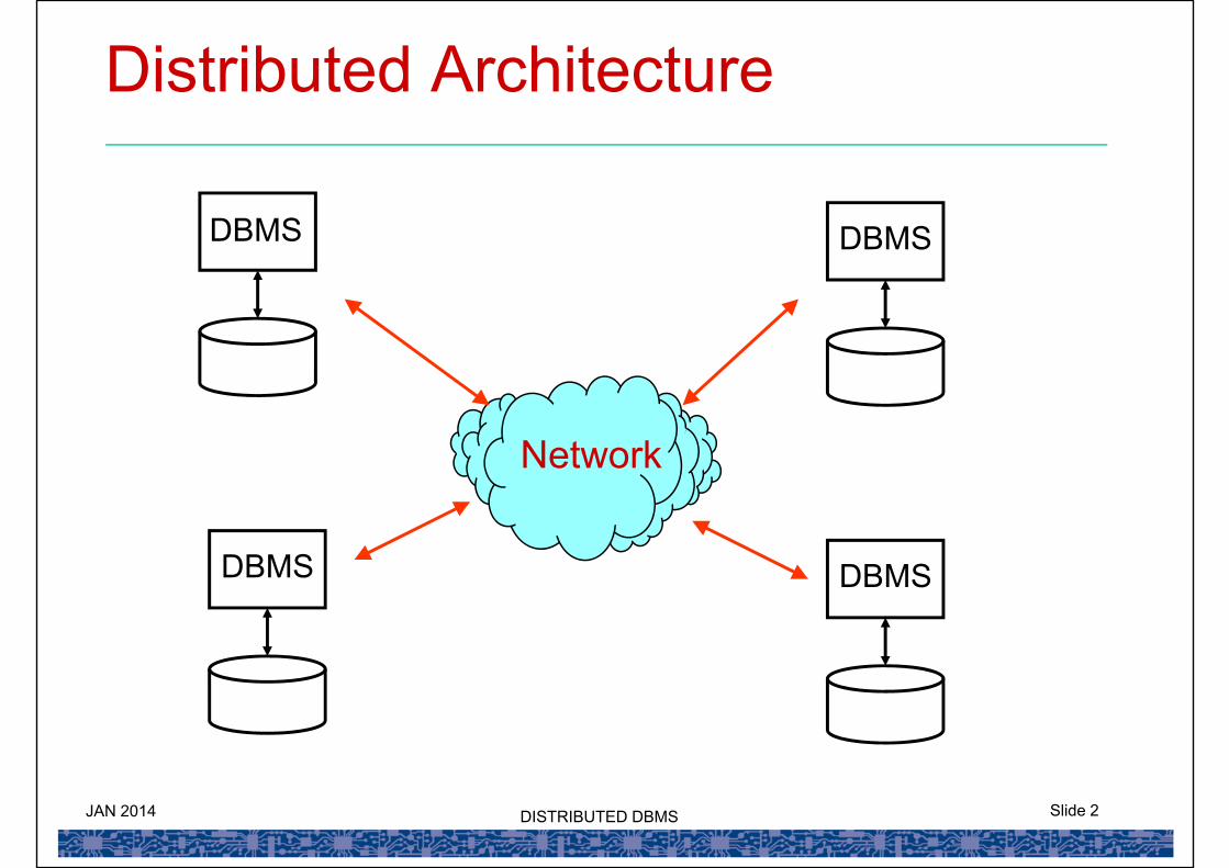
Distributed Architecture

Network

DBMS DBMS

DBMS DBMS


ADVANTAGES

• Availability• Locality • Reliability• Parallelism• Load Balancing• Scalability• Autonomy


DISADVANTAGES

• Significantly more complex to program and to maintain

• Communication costs need to be taken into account

• Communication failures need to be handled


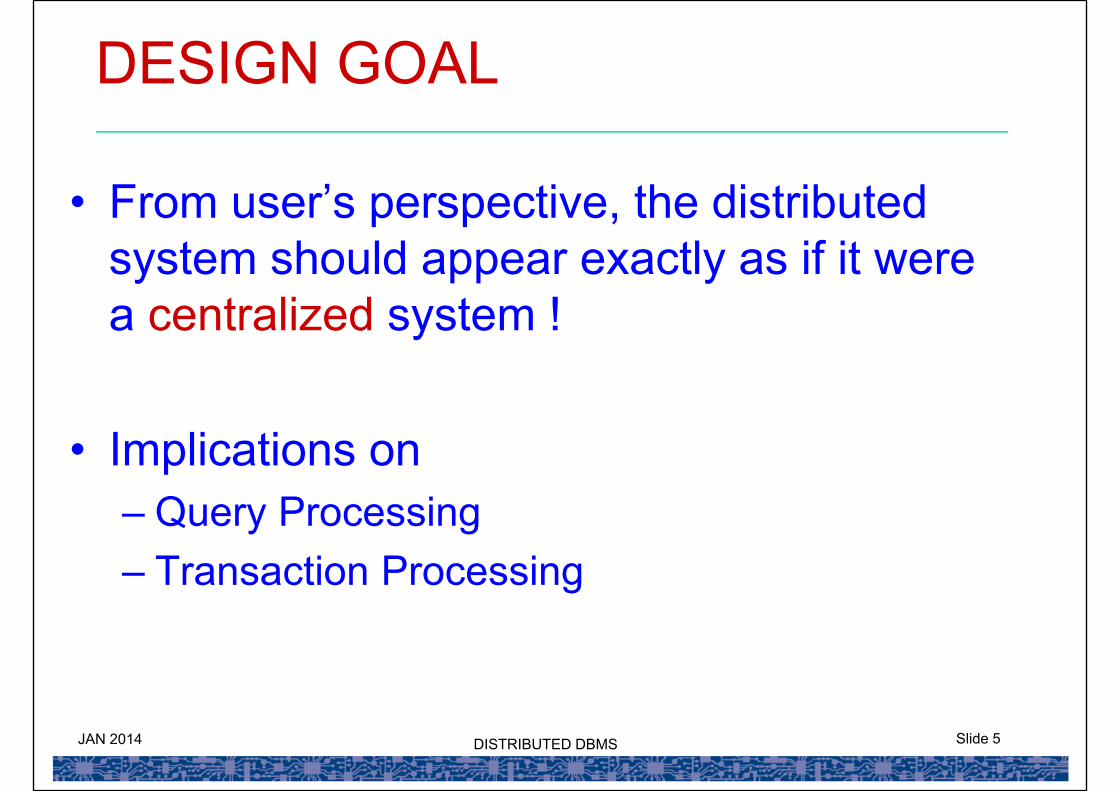
DESIGN GOAL

• From user’s perspective, the distributed system should appear exactly as if it werea centralized system !

• Implications on– Query Processing– Transaction Processing


Distributed Query Processing


Problem Complexity

• In centralized, performance metric was number of disk accesses

• In distributed, disk accesses and communication cost have to be taken into account

• Plan space explodes since location also becomes a parameter


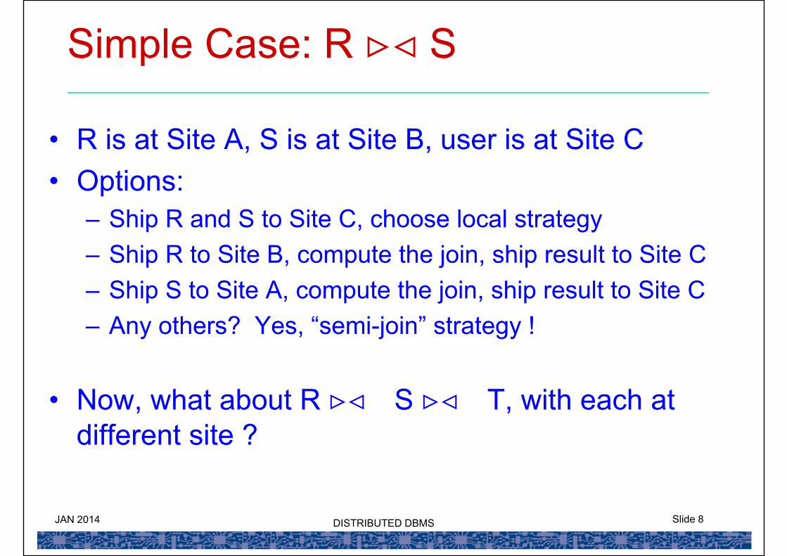
Simple Case: R S

• R is at Site A, S is at Site B, user is at Site C• Options:

– Ship R and S to Site C, choose local strategy– Ship R to Site B, compute the join, ship result to Site C– Ship S to Site A, compute the join, ship result to Site C– Any others? Yes, “semi-join” strategy !

• Now, what about R S T, with each at different site ?


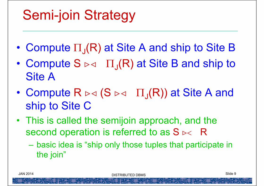
Semi-join Strategy

• Compute J(R) at Site A and ship to Site B• Compute S J(R) at Site B and ship to

Site A• Compute R (S J(R)) at Site A and

ship to Site C• This is called the semijoin approach, and the

second operation is referred to as S R– basic idea is “ship only those tuples that participate in

the join”


Proof of Correctness

R (S J(R))= (R J(R)) S

– because of associativity/commutativity properties

= R S


Cost Computation Factors

• Disk Cost• Communication Cost• Meta-data shipping or re-creation Cost !!!


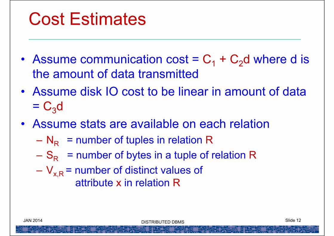
Cost Estimates

• Assume communication cost = C1 + C2d where d is the amount of data transmitted

• Assume disk IO cost to be linear in amount of data = C3d

• Assume stats are available on each relation– NR = number of tuples in relation R– SR = number of bytes in a tuple of relation R– Vx,R = number of distinct values of

attribute x in relation R


R S

• Relation R (x,y) at Site A• Relation S (y,z) at Site B• Stats:

– NR = 128, NS = 256– Vy,R = 32, Vy,S = 128– SR = 10, SS = 10

• Results required at Site A


Strategy 1

• Ship S to Site A and compute join with R.• Cost:

– Retrieve S from disk: C3 (NSSs) = 2560 C3

– Ship S to Site A: C1 + C2 (NSSS) = C1 + 2560 C2

– Store S at Site A: C3 (NSSs) = 2560 C3

– nested-loop tuple join:C3 (NRSR + NR (NSSS)) = 328960 C3• (note that smaller relation, R, is outer)


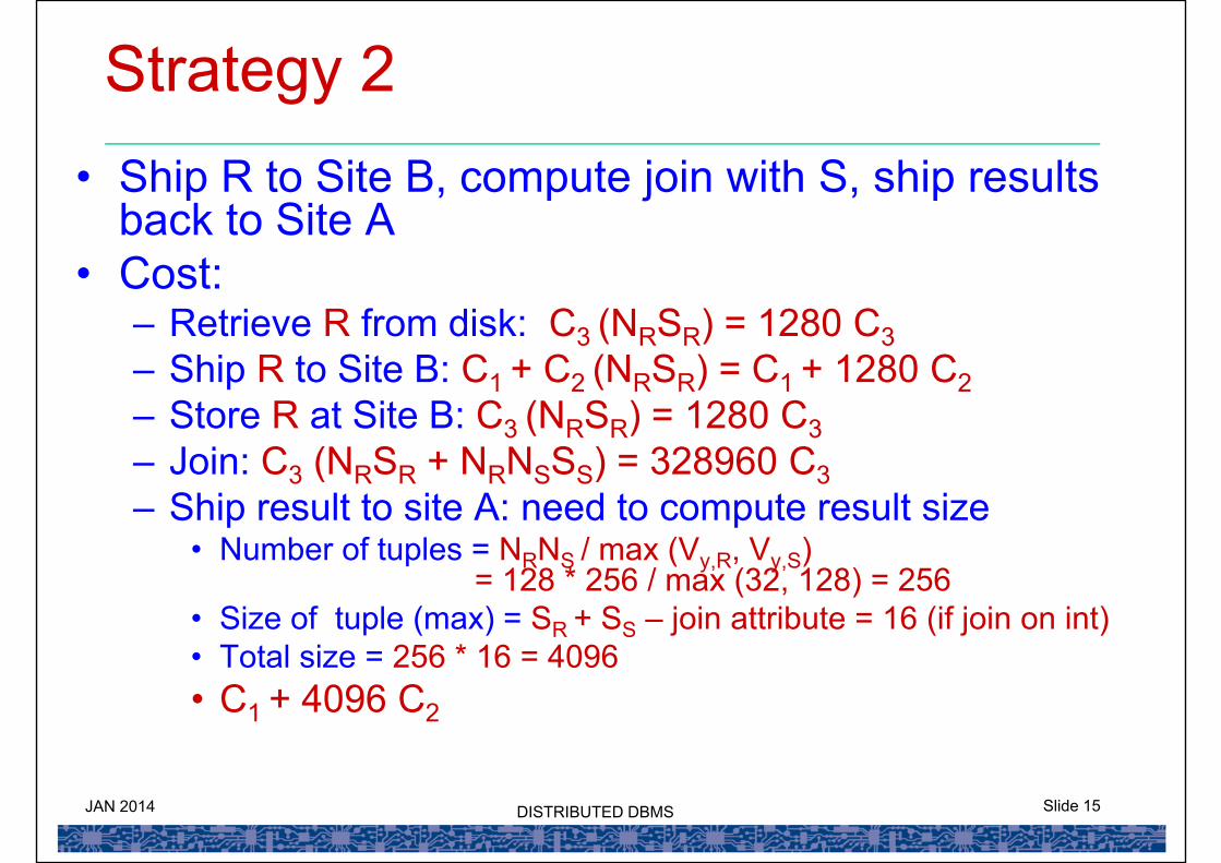
Strategy 2• Ship R to Site B, compute join with S, ship results

back to Site A• Cost:

– Retrieve R from disk: C3 (NRSR) = 1280 C3– Ship R to Site B: C1 + C2 (NRSR) = C1 + 1280 C2– Store R at Site B: C3 (NRSR) = 1280 C3– Join: C3 (NRSR + NRNSSS) = 328960 C3– Ship result to site A: need to compute result size

• Number of tuples = NRNS / max (Vy,R, Vy,S)= 128 * 256 / max (32, 128) = 256

• Size of tuple (max) = SR + SS – join attribute = 16 (if join on int)• Total size = 256 * 16 = 4096• C1 + 4096 C2


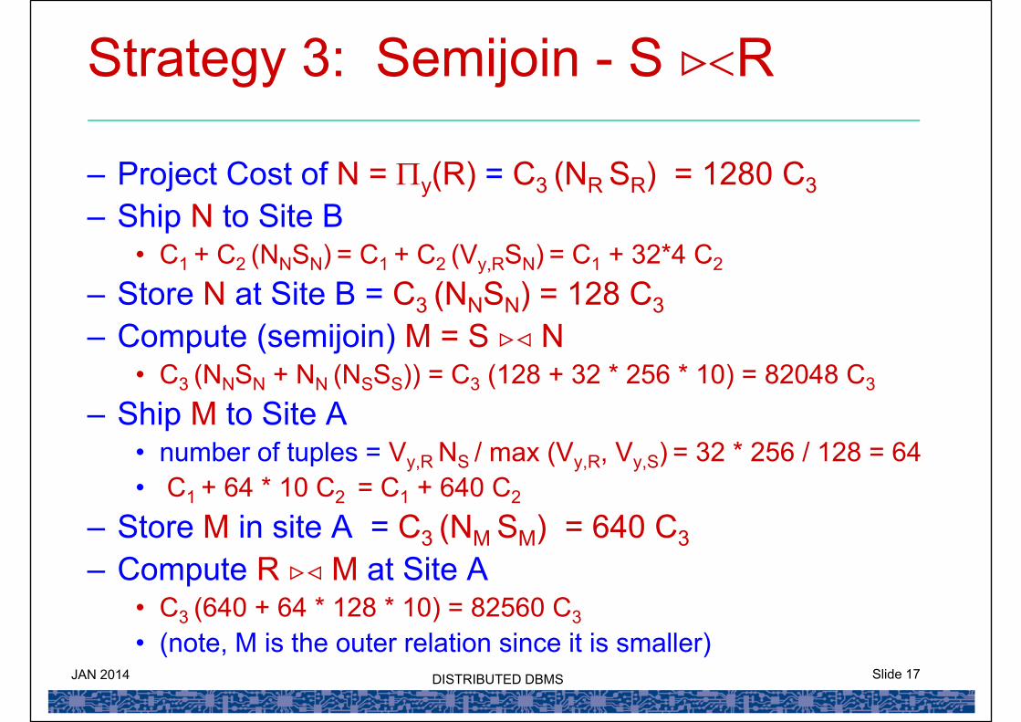
Strategy 3: Semijoin - S R

– Project Cost of N = y(R) = C3 (NR SR) = 1280 C3 – Ship N to Site B

• C1 + C2 (NNSN) = C1 + C2 (Vy,RSN) = C1 + 32*4 C2

– Store N at Site B = C3 (NNSN) = 128 C3– Compute (semijoin) M = S N

• C3 (NNSN + NN (NSSS)) = C3 (128 + 32 * 256 * 10) = 82048 C3

– Ship M to Site A• number of tuples = Vy,R NS / max (Vy,R, Vy,S) = 32 * 256 / 128 = 64• C1 + 64 * 10 C2 = C1 + 640 C2

– Store M in site A = C3 (NM SM) = 640 C3– Compute R M at Site A

• C3 (640 + 64 * 128 * 10) = 82560 C3 • (note, M is the outer relation since it is smaller)


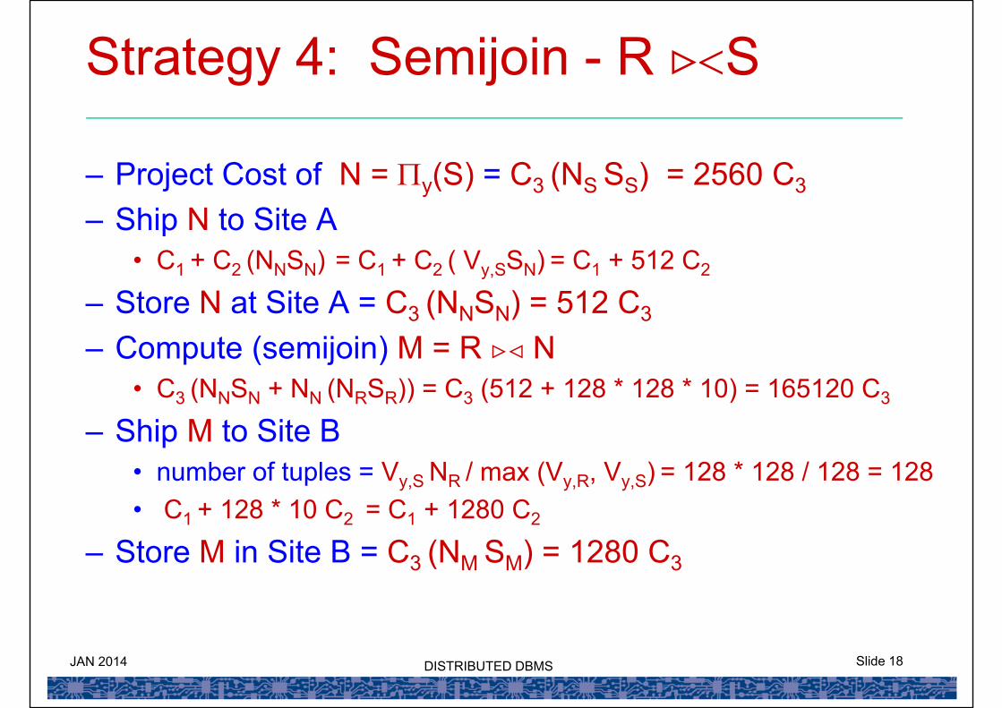
Strategy 4: Semijoin - R S

– Project Cost of N = y(S) = C3 (NS SS) = 2560 C3

– Ship N to Site A• C1 + C2 (NNSN) = C1 + C2 ( Vy,SSN) = C1 + 512 C2

– Store N at Site A = C3 (NNSN) = 512 C3

– Compute (semijoin) M = R N• C3 (NNSN + NN (NRSR)) = C3 (512 + 128 * 128 * 10) = 165120 C3

– Ship M to Site B• number of tuples = Vy,S NR / max (Vy,R, Vy,S) = 128 * 128 / 128 = 128• C1 + 128 * 10 C2 = C1 + 1280 C2

– Store M in Site B = C3 (NM SM) = 1280 C3


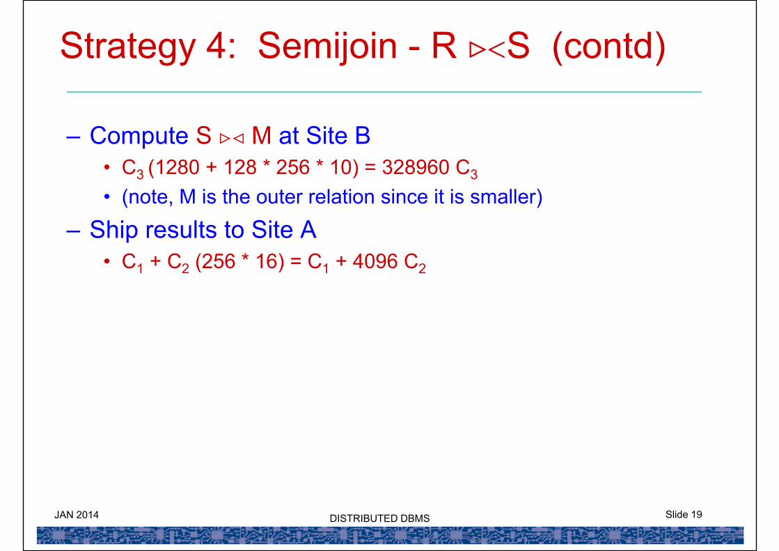
Strategy 4: Semijoin - R S (contd)

– Compute S M at Site B• C3 (1280 + 128 * 256 * 10) = 328960 C3

• (note, M is the outer relation since it is smaller)

– Ship results to Site A• C1 + C2 (256 * 16) = C1 + 4096 C2


Cost Comparison

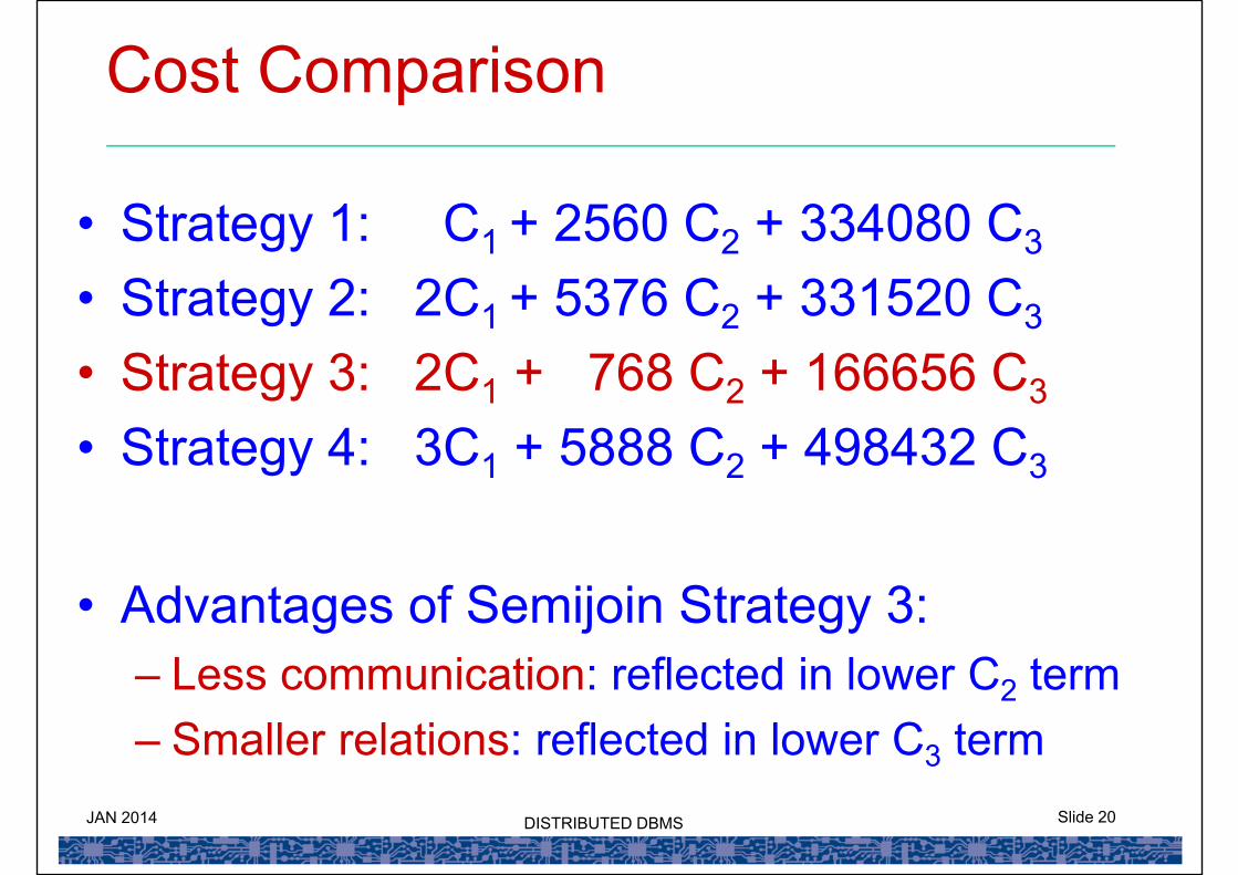
• Strategy 1: C1 + 2560 C2 + 334080 C3

• Strategy 2: 2C1 + 5376 C2 + 331520 C3

• Strategy 3: 2C1 + 768 C2 + 166656 C3

• Strategy 4: 3C1 + 5888 C2 + 498432 C3

• Advantages of Semijoin Strategy 3:– Less communication: reflected in lower C2 term– Smaller relations: reflected in lower C3 term


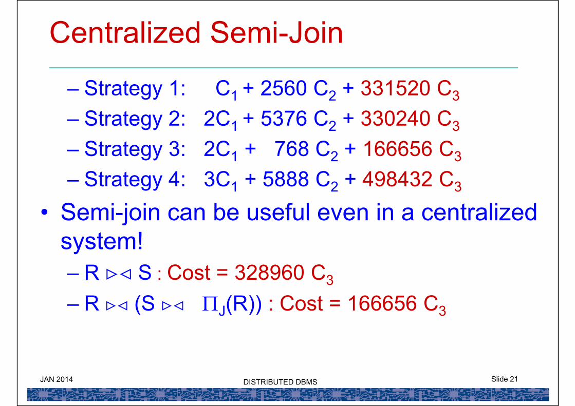
Centralized Semi-Join

– Strategy 1: C1 + 2560 C2 + 331520 C3

– Strategy 2: 2C1 + 5376 C2 + 330240 C3

– Strategy 3: 2C1 + 768 C2 + 166656 C3

– Strategy 4: 3C1 + 5888 C2 + 498432 C3

• Semi-join can be useful even in a centralized system!– R S : Cost = 328960 C3

– R (S J(R)) : Cost = 166656 C3


Distributed Transaction Processing


Execution Model DBMS

DBMS DBMS DBMS....Network

Master

CohortCohort


Guaranteeing ACID

• Each cohort site can guarantee local ACID using the standard 2PL + WAL combination

• But, does “local ACID global ACID” ?• No! For example, all sites may not

implement the same decision (commit/abort)• Therefore, need a commit protocol to ensure

uniform decision across all sites participating in the distributed execution of the transaction


Two-Phase Commit Protocol

• 2PC guarantees global atomicity

• Note, 2PC different from 2PL !


Transaction Execution

• Master sends STARTWORK messages to the cohorts along with the associated work (this can be either sequential or in parallel)

• A cohort after completing its work sends a WORKDONE message to the master.

• The 2PC protocol is initiated by the master after the “data processing” part of the transaction is completed


Phase I: Obtaining a decision

• Master asks all cohorts to prepare to commit transaction T.– sends prepare T messages to all sites at which T executed

• Upon receiving message, transaction manager at each site determines if it can commit the transaction– if not, add a record <abort T> to the log and send abort T message

to master– if the transaction can be committed, then:

• add the record <ready T> to the log• force all log records for T to stable storage• send ready T message to master


Phase II: Recording the Decision

• T can be committed if master received a ready T message from all cohorts; otherwise T must be aborted.

• Master adds a decision record, <commit T> or <abort T>,to the log and forces record onto stable storage.

• Master sends a message to each cohort informing it of the decision (commit or abort)

• The cohorts take appropriate action locally by writing the log records and send an <ack T> message to master.

• After receiving all ACK messages, the master writes an <end T> log record and then “forgets” the transaction.


2PC Protocol

MASTER

<Phase I>

• log* (commit / abort)

<Phase II>

• log (end)

COHORT

• log* (ready / abort)

• log* (commit / abort)

ready T / abort T

prepare T

decision T(to ready cohorts)

ack T


TYPES OF FAILURES

• Cohort Site Failure

• Master Site Failure

• Network Partition


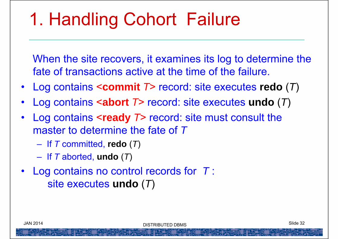
1. Handling Cohort Failure

When the site recovers, it examines its log to determine the fate of transactions active at the time of the failure.

• Log contains <commit T> record: site executes redo (T)• Log contains <abort T> record: site executes undo (T)• Log contains <ready T> record: site must consult the

master to determine the fate of T– If T committed, redo (T)– If T aborted, undo (T)

• Log contains no control records for T : site executes undo (T)


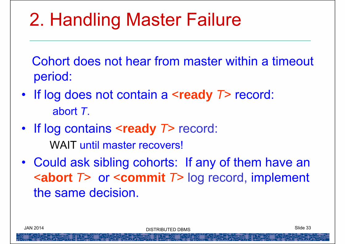
2. Handling Master Failure

Cohort does not hear from master within a timeout period:

• If log does not contain a <ready T> record:abort T.

• If log contains <ready T> record:WAIT until master recovers!

• Could ask sibling cohorts: If any of them have an <abort T> or <commit T> log record, implement the same decision.


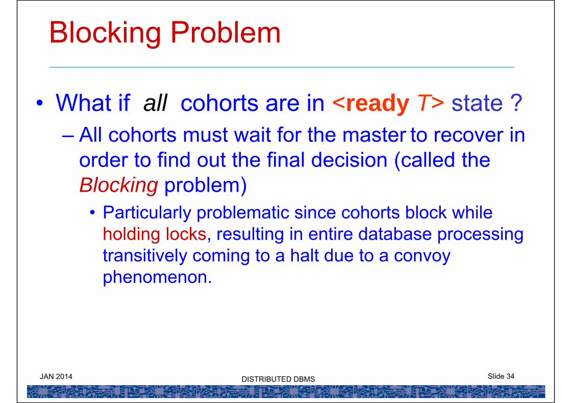
Blocking Problem

• What if all cohorts are in <ready T> state ?– All cohorts must wait for the master to recover in

order to find out the final decision (called the Blocking problem)

• Particularly problematic since cohorts block while holding locks, resulting in entire database processing transitively coming to a halt due to a convoy phenomenon.


3.Handling Network Partition Failure

• If master and all cohorts remain in one partition, the failure has no effect on the commit protocol.

• If master and cohorts are spread across partitions:– Sites not in the partition containing the master think master has

failed, and execute the protocol to deal with master failure.• No harm results, but sites may still have to wait for decision from

master.– Master and the sites in its partition think that the sites in the other

partition have failed, and follow the usual commit protocol.• Again, no harm results


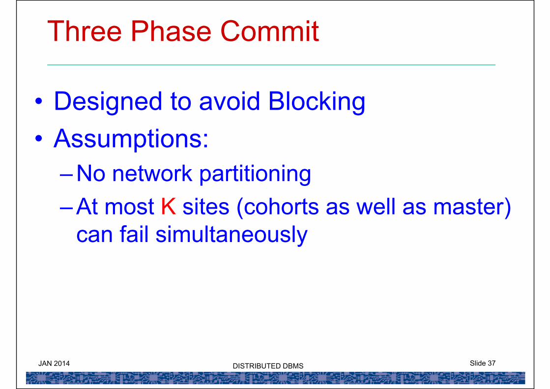
Three Phase Commit

• Designed to avoid Blocking• Assumptions:

– No network partitioning– At most K sites (cohorts as well as master)

can fail simultaneously


Concurrency Control


Concurrency Control

• If all sites individually follow basic 2PL, is there any problem ?

• Yes, could have different serial orders at different sites!


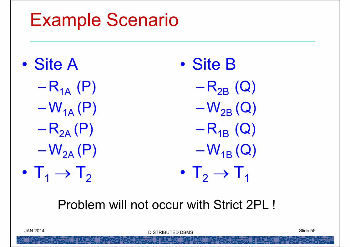
Example Scenario

• Site A– R1A (P)– W1A (P)– R2A (P)– W2A (P)

• T1 T2

• Site B– R2B (Q)– W2B (Q)– R1B (Q)– W1B (Q)

• T2 T1

Problem will not occur with Strict 2PL !


Concurrency Control (contd)

• So, simple solution is to use strict 2PL at all the sites hosting the distributed DBMS.

• Note that above is assuming single copy of alldata items, i.e. no replicas.

• If there are replicas, numerous techniques for handling concurrency control (“read any, write all”, “primary copy”, “majority vote”, ...)– Full book on this topic:

Concurrency Control and Recovery in Database SystemsP. Bernstein, V. Hadzilacos, N. GoodmanAddison-Wesley, 1987


END DISTRIBUTED DATABASES

E0 261

DISTRIBUTED DATABASES

Documents

Transcript of DISTRIBUTED DATABASES