commercial transactions in a nutshell for kenyan law students
Upload
khangminh22Category
view
0download
0
Distributed Databases in a Nutshell
Marc [email protected]
Department of InformaticsUniversity of Fribourg, Switzerland
Priciples of Distributed Database SystemsM. T. Ozsu, P. Valduriez
Prentice Hall
February 2005DDBMS – p.1/39
Motivation
Why distributed applications at all ?
Correspond to today’s enterprise structures.Distributed computer technologyReliabilityDivide-and-Conquer, ParallelismEconomical reasons
DDBMS – p.2/39

Motivation
Why distributed applications at all ?
Correspond to today’s enterprise structures.Distributed computer technologyReliabilityDivide-and-Conquer, ParallelismEconomical reasons
What is distributed ?
Processing logicFunctions (special functions delegated to special HW)DataControl of execution
! All points are unified in the case of distributed databases.
DDBMS – p.2/39

Definitions
Distributed Database System (DDBS)A collection of multiple, logically interrelated databases distributed over anetwork.
Distributed Database Management System (DDBMS)Software system that permits the management of the DDBS and makesthe distribution transparent to the user.
DDBMS – p.3/39

Definitions
Distributed Database System (DDBS)A collection of multiple, logically interrelated databases distributed over anetwork.
Distributed Database Management System (DDBMS)Software system that permits the management of the DDBS and makesthe distribution transparent to the user.
DDBMS – p.3/39

Outlook I
This talk deals with:
Promises and New Problem Areas of a DDBMS
Architectures and Design of DDBMSs
Distribution design issuesFragmentationAllocation
Distributed query processingQuery decompositionData locationGlobal & local query optimization
What is expected to know:
Relation algebra, normal forms & relational calculus (SQL)
DDBMS – p.4/39
Outlook II
This talk does NOT deal with:
Relational algebra & relational calculus
Semantic data controlView managementData securityIntegrity control
Transaction management
Distribution concurrency control
Distributed DB reliability
Distributed non-relational DB & interoperability
DDBMS – p.5/39

Promises of DDBMSs I
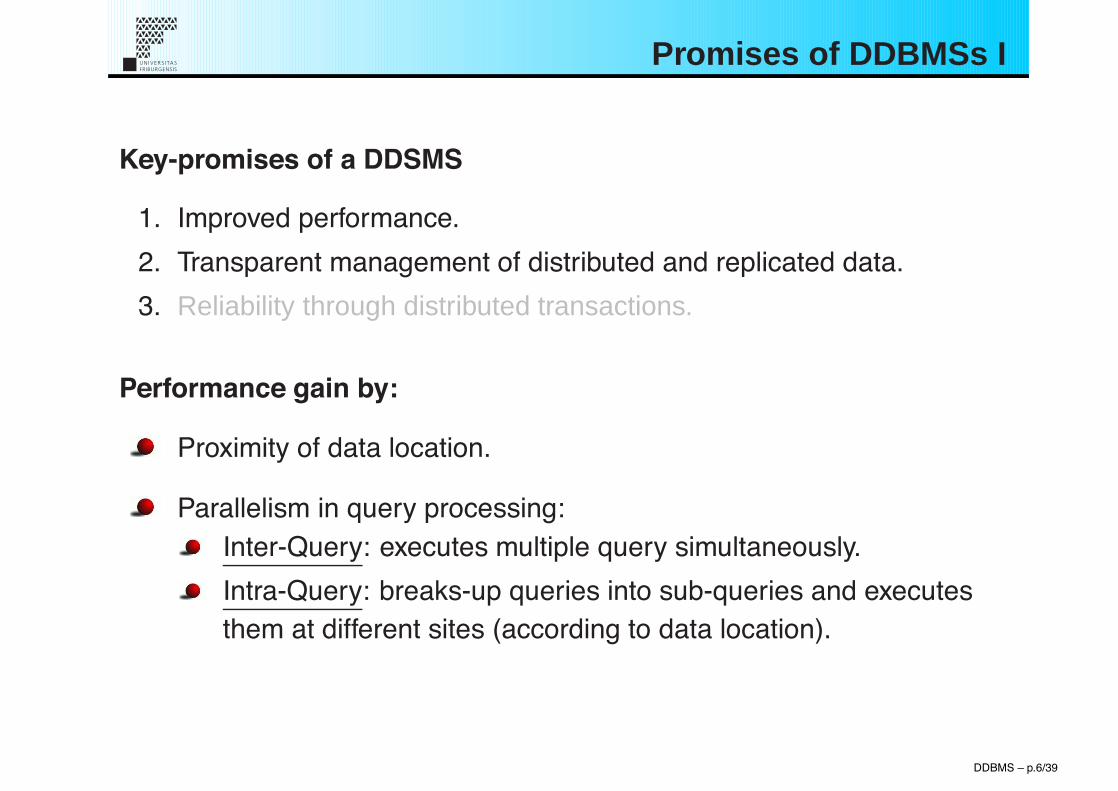
Key-promises of a DDSMS
1. Improved performance.2. Transparent management of distributed and replicated data.3. Reliability through distributed transactions.
DDBMS – p.6/39
Promises of DDBMSs I
Key-promises of a DDSMS
1. Improved performance.2. Transparent management of distributed and replicated data.3. Reliability through distributed transactions.
Performance gain by:
Proximity of data location.
Parallelism in query processing:Inter-Query: executes multiple query simultaneously.Intra-Query: breaks-up queries into sub-queries and executesthem at different sites (according to data location).
DDBMS – p.6/39

Promises of DDBMSs II
Types of transparency:
Data transparencyLogical data independence" immunity of user app. to changes in logical DB structure.Physical data independence" hiding details of storage structure.
DDBMS – p.7/39

Promises of DDBMSs II
Types of transparency:
Data transparencyLogical data independence" immunity of user app. to changes in logical DB structure.Physical data independence" hiding details of storage structure.
Network transparency = Distribution transparency" hiding existence of the network.
Replication transparency" hiding existence & handling of copies.
Fragmentation transparency" hiding existence & handling of fragmented data.
DDBMS – p.7/39

New Problem Areas & Challenges
New problem areas implied by distribution:
Full replication vs. partial replication vs. no replicationDegree & strategy of fragmentationData distribution and relocationDistributed query processingDistributed directory management (metadata)
Distributed concurrency control
Reliability, crash recovery
Network problems
Heterogeneous DB
OS support problems
! These areas are not isolated one from another ...DDBMS – p.8/39

Architectures and design of DDBMSs I
Architectures are classified by:AutonomityDistributionHeterogeneity
DDBMS – p.9/39

Architectures and design of DDBMSs I
Architectures are classified by:AutonomityDistributionHeterogeneity
Autonomity of DDBMSs:Distribution of control (not data). Degree of which individual DBMSs canoperate independently " 3 dimensions of autonomity:
tight integrationsemiautonomous systemtotal isolation
DDBMS – p.9/39

Architectures and design of DDBMSs II
Distribution of DDBMSs:Distribution of data " 3 dimensions of distribution:
no distributionclient / server (only servers have DB functionality)peer-to-peer (full distribution)
Heterogeneity of DDBMSs:Heterogeneity of data model and query language " 2 dimensions ...
peer-to-peer distributed homogeneous DBMS
client-server distributed homogeneous DBMS
DDBMS – p.10/39

ANSI Component Design Model
Component description:
1. Interpretation of user commands and out-put formatting.
2. Tests integrity constraints, authorization.Solvability of user query.
3. Determines execution strategy (minimizecost function). Translates global query intolocal ones.
4. Coordinates execution of distributed userqueries. Communicates with other 4s.
5. Chooses best data access path.
6. Ensures consistency of DB.
7. Physical access to DB. Buffering.DDBMS – p.11/39
Fragmentation: Motivation
Relation is not a suitable unit of distribution.
DDBMS – p.12/39

Fragmentation: Motivation
Relation is not a suitable unit of distribution.
Application views are subsets of relations.
If multiple, distributed application access the same relation:a) Relation is not replicated.
! High volume of remote data access.b) Relation is replicated.
! High storage use & update problems.
Allow multiple transactions and parallel query execution.! Increases level of concurrency.
Alternatives of fragmentation:
horizontal fragmentation & vertical fragmentationhybrid fragmentation
DDBMS – p.12/39

Fragmentation: A first look
Key Name Population Life
c1 France 58973000 78.5c2 Germany 82037000 77.5c3 Switzerland 7124000 79.5c4 Italy 57613000 78.4
Key Name Population Life
c1 France 58973000 78.5c2 Germany 82037000 77.5
Key Name Population Life
c3 Switzerland 7124000 79.5c4 Italy 57613000 78.4
Key Name
c1 Francec2 Germanyc3 Switzerlandc4 Italy
Key Population Life
c1 58973000 78.5c2 82037000 77.5c3 7124000 79.5c4 57613000 78.4
DDBMS – p.13/39

Fragmentation: A first look
Key Name Population Life
c1 France 58973000 78.5c2 Germany 82037000 77.5c3 Switzerland 7124000 79.5c4 Italy 57613000 78.4
Key Name Population Life
c1 France 58973000 78.5c2 Germany 82037000 77.5
!
Key Name Population Life
c3 Switzerland 7124000 79.5c4 Italy 57613000 78.4
Key Name
c1 Francec2 Germanyc3 Switzerlandc4 Italy
!"Key
Key Population Life
c1 58973000 78.5c2 82037000 77.5c3 7124000 79.5c4 57613000 78.4
DDBMS – p.13/39

Fragmentation II
Disadvantages of fragmentation:
Performance problem if an application uses multiple non-mutualexclusive fragments.Integrity control over multiple sites.
DDBMS – p.14/39
Fragmentation II
Disadvantages of fragmentation:
Performance problem if an application uses multiple non-mutualexclusive fragments.Integrity control over multiple sites.
Degree of fragmentation:
no fragmentation vs. full fragmentation (atomic tuples or columns).
! compromise with respect to some parameters ...
Correctness rules of fragmentation:
Averts semantic changes during fragmentation.
Completeness (lost-less decomposition)
Reconstruction: R =!
Ri vs. R = !"Key Ri
Disjointness (for vertical fragmentation on non-key attributes).DDBMS – p.14/39

Horizontal Fragmentation I
Fragmentation requires database informations (metadata).
There are two types of relations: OWNER and MEMBER.
Li are called LINKS.Ex: owner(L1) = Country Relation, member(L1) = City Relation
Important are those owner which are not member of any link.
DDBMS – p.15/39
Horizontal Fragmentation II
2 Ways of Horizontal Fragmentation (HF)
primary HF: for owner - Relationsderived HF: for member - Relations
DDBMS – p.16/39

Horizontal Fragmentation II
2 Ways of Horizontal Fragmentation (HF)
primary HF: for owner - Relationsderived HF: for member - Relations
An important note:
Links are equi-joins # Joins over attributes with only ”=” predicates.
Name P ·103
F 58973DE 82037CH 7124I 57613
!"
City Country % P
Paris F 3.6
Berlin DE 4.1
Rome I 4.6
=
Country City P ·103 % P
F Paris 58973 3.6
DE Berlin 82037 4.1
I Rome 57613 4.6
Country !" Country.Name = City.Country City
DDBMS – p.16/39
Primary Horizontal Fragmentation I
Definition Simple Predicate:For a relation R(A1, . . . , An), d(Ai) = di, a simple predicat pj has the formpj : Ai # value, where # $ {=, %=, >, <,&,'} and value $ di.
DDBMS – p.17/39

Primary Horizontal Fragmentation I
Definition Simple Predicate:For a relation R(A1, . . . , An), d(Ai) = di, a simple predicat pj has the formpj : Ai # value, where # $ {=, %=, >, <,&,'} and value $ di.
Definition Minterm Predicate:CNF of simple predicates.
DDBMS – p.17/39

Primary Horizontal Fragmentation I
Definition Simple Predicate:For a relation R(A1, . . . , An), d(Ai) = di, a simple predicat pj has the formpj : Ai # value, where # $ {=, %=, >, <,&,'} and value $ di.
Definition Minterm Predicate:CNF of simple predicates.
Horizontal fragmentation of R consists of all tuples in R satisfying a givenminterm predicate.
Ri = $mi(R)
where mi is the minterm predicate to obtain Ri.
! Given a set of minterm predicates, there are as many horizontalfragments as minterms in this set! minterm fragments.
DDBMS – p.17/39

Primary Horizontal Fragmentation II
2 important aspects of simple predicates: completeness & minimality
DDBMS – p.18/39

Primary Horizontal Fragmentation II
2 important aspects of simple predicates: completeness & minimality
Completeness of simple predicates:A set of simple predicates Pr is said to be complete if and only if there isan equal probability of access by every application to any tuple belongingto any minterm fragment defined by Pr.
DDBMS – p.18/39

Primary Horizontal Fragmentation III
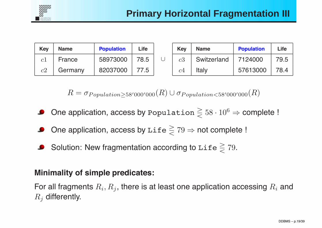
Key Name Population Life
c1 France 58973000 78.5c2 Germany 82037000 77.5
Key Name Population Life
c3 Switzerland 7124000 79.5c4 Italy 57613000 78.4
R = $Population!58!000!000(R) ( $Population<58!000!000(R)
One application, access by Population ! 58 · 106 ! complete !
One application, access by Life ! 79 ! not complete !
Solution: New fragmentation according to Life ! 79.
DDBMS – p.19/39
Primary Horizontal Fragmentation III
Key Name Population Life
c1 France 58973000 78.5c2 Germany 82037000 77.5
!
Key Name Population Life
c3 Switzerland 7124000 79.5c4 Italy 57613000 78.4
R = $Population!58!000!000(R) ( $Population<58!000!000(R)
One application, access by Population ! 58 · 106 ! complete !
One application, access by Life ! 79 ! not complete !
Solution: New fragmentation according to Life ! 79.
Minimality of simple predicates:For all fragments Ri, Rj , there is at least one application accessing Ri andRj differently.
DDBMS – p.19/39

Primary Horizontal Fragmentation IV
Consequence of completeness & minimality:completeness! fragments are logically uniform.minimality! simple predicates do not produce unused fragments.
DDBMS – p.20/39

Primary Horizontal Fragmentation IV
Consequence of completeness & minimality:completeness! fragments are logically uniform.minimality! simple predicates do not produce unused fragments.
Determining the minterms is trivial ! But this set may be quite large ...
Fortunately, the set of minterms can be reduced.
This elimination is performed by identifying those minterms that might bycontradictory to a set of implications I.
DDBMS – p.20/39

Primary Horizontal Fragmentation V
Example: Attribute A with domain dA = {v1, v2}. Let P = {p1, p2} be aset of simple predicates,p1 : A = v1
p2 : A = v2
We build the set of possible minterms:m1 : (A = v1) ) (A = v2) m3 : ¬(A = v1) ) (A = v2)
m2 : (A = v1) ) ¬(A = v2) m4 : ¬(A = v1) ) ¬(A = v2)
Clearly, m1 and m2 can be eliminated; they contradict to I.The implication i $ I eliminating m1 is:i : (A = v1) ! ¬(A = v2)
DDBMS – p.21/39

Derived Horizontal Fragmentation I
owner-relations are fragmented according to the user queries.member-relations depend on their owner(s).
Let L be a link. owner(L) = S and member(L) = R.We want to fragment R.
Ri = R ! Si
DDBMS – p.22/39

Derived Horizontal Fragmentation I
owner-relations are fragmented according to the user queries.member-relations depend on their owner(s).
Let L be a link. owner(L) = S and member(L) = R.We want to fragment R.
Ri = R ! Si
This is a semi-join. It results in the subset of tuples in R that participate inthe join of R and Si. Formally,
Ri = R ! Si = %A(R "! Si)
where A is the domain of R.
! Given the primary fragmentation, derived fragmentation is simple !
DDBMS – p.22/39

Derived Horizontal Fragmentation II
Often, a member has multiple owners ! there are multiple possibilities forderived fragmentation (according to each of the owners).
Choose the fragmentation1. with better join-characteristics.2. that is used in more applications.
! Optimization problem.
DDBMS – p.23/39

Derived Horizontal Fragmentation II
Often, a member has multiple owners ! there are multiple possibilities forderived fragmentation (according to each of the owners).
Choose the fragmentation1. with better join-characteristics.2. that is used in more applications.
! Optimization problem.
Criteria 1 has 2 motivations:Join on fragments is faster than on main relation itself.Fragments allow parallel query execution.
Criteria 2 facilitates the access of heavy users such that their totalimpact on the system is minimized.
DDBMS – p.23/39
Vertical Fragmentation
Produces fragments R1, R2, . . . , Rn of R, each one containing a subset ofR’s attributes and it’s primary key.
DDBMS – p.24/39

Vertical Fragmentation
Produces fragments R1, R2, . . . , Rn of R, each one containing a subset ofR’s attributes and it’s primary key.
More complicated than horizontal fragmentation:HF: n simple predicates! 2n possible minterms = #fragments.A lot of them can be eliminated.VF: m non-primary key attributes! B(m) #= mm fragments (m-thBell number).
No optimal solution! heuristics.Grouping: Starts by assigning each attribute to one fragment and ateach step, joins some fragments.Splitting: Starts with a relations and splits according to the accessbehavior of applications for each attribute.
DDBMS – p.24/39

Hybrid Fragmentation
Tree-structured partitioning ...
Level of nesting can be large - but in practice, levels do rarely exceed 2,because normalized relations are already small.
DDBMS – p.25/39

The Allocation Problem
Set of fragments F = {F1, F2, . . . , Fn}, network consisting of sitesS = {S1, S2, . . . , Sm} and applications Q = {q1, q2, . . . , qq}.
! Optimal distribution of F to S regarding Q.
DDBMS – p.26/39

The Allocation Problem
Set of fragments F = {F1, F2, . . . , Fn}, network consisting of sitesS = {S1, S2, . . . , Sm} and applications Q = {q1, q2, . . . , qq}.
! Optimal distribution of F to S regarding Q.
Optimality is defined with respect to:
Minimal costs ofstoring Fi at Sj
querying Fi at Sj
updating Fj
data communication
Performanceminimize response time of Si
maximize system throughput
! Problem is NP-Complete
There are no general models which take a set of fragments as input and produce a nearoptimal allocation. All existing models make some assumptions to simplify the problem andare applicable only to certain specific formulations.
DDBMS – p.26/39

Query Processing Overview
Transformation high-level query" low-level query.High-level queries typically in relation calculus (SQL-Expression).Low-level queries in relation algebra + communication primitives.
DDBMS – p.27/39

Query Processing Overview
Transformation high-level query" low-level query.High-level queries typically in relation calculus (SQL-Expression).Low-level queries in relation algebra + communication primitives.
In centralized databases ...
Find best relational algebra query among all equivalent transformations! computationally intractable! Heuristics
In distributed databases ...
Additionally select the best site to process data and minimize networktraffic! Increases solution space and problem complexity.
DDBMS – p.27/39

Query Processing Example I
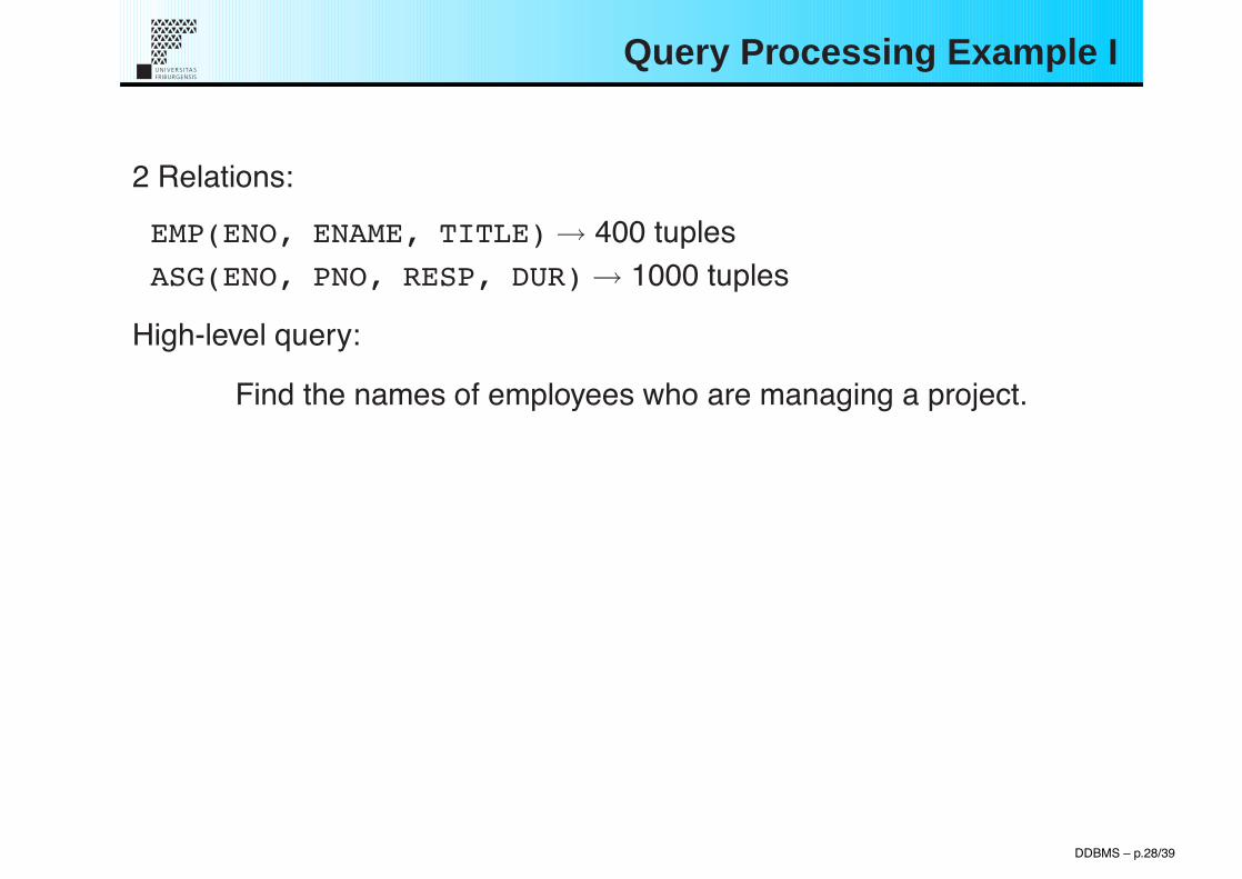
2 Relations:EMP(ENO, ENAME, TITLE)" 400 tuplesASG(ENO, PNO, RESP, DUR) " 1000 tuples
DDBMS – p.28/39
Query Processing Example I
2 Relations:EMP(ENO, ENAME, TITLE)" 400 tuplesASG(ENO, PNO, RESP, DUR) " 1000 tuples
High-level query:
Find the names of employees who are managing a project.
DDBMS – p.28/39
Query Processing Example I
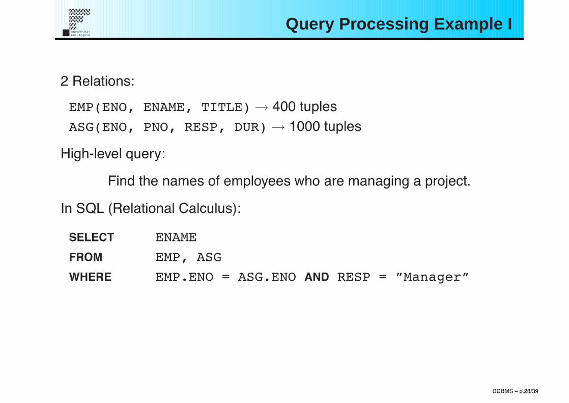
2 Relations:EMP(ENO, ENAME, TITLE)" 400 tuplesASG(ENO, PNO, RESP, DUR) " 1000 tuples
High-level query:
Find the names of employees who are managing a project.
In SQL (Relational Calculus):
SELECT ENAMEFROM EMP, ASGWHERE EMP.ENO = ASG.ENO AND RESP = ”Manager”
DDBMS – p.28/39

Query Processing Example I
2 Relations:EMP(ENO, ENAME, TITLE)" 400 tuplesASG(ENO, PNO, RESP, DUR) " 1000 tuples
High-level query:
Find the names of employees who are managing a project.
In SQL (Relational Calculus):
SELECT ENAMEFROM EMP, ASGWHERE EMP.ENO = ASG.ENO AND RESP = ”Manager”
2 equivalent low-level queries:
1."ENAME($RESP = !!Manager!! " EMP.ENO = ASG.ENO (EMP* ASG)
2."ENAME(EMP "!ENO ($RESP = !!Manager!!(ASG)))
DDBMS – p.28/39

Query Processing Example II
Clearly, the second transformation is better (avoids Carthesian product).We assume that both relations are horizontally fragmented.
EMP1 = $ENO # !!E3!!(EMP) stored at site 1.EMP2 = $ENO > !!E3!!(EMP) stored at site 2.ASG1 = $ENO # !!E3!!(ASG) stored at site 3.ASG2 = $ENO > !!E3!!(ASG) stored at site 4.
The result of the query is expected at site 5.
DDBMS – p.29/39

Query Processing Example II
Clearly, the second transformation is better (avoids Carthesian product).We assume that both relations are horizontally fragmented.
EMP1 = $ENO # !!E3!!(EMP) stored at site 1.EMP2 = $ENO > !!E3!!(EMP) stored at site 2.ASG1 = $ENO # !!E3!!(ASG) stored at site 3.ASG2 = $ENO > !!E3!!(ASG) stored at site 4.
The result of the query is expected at site 5.
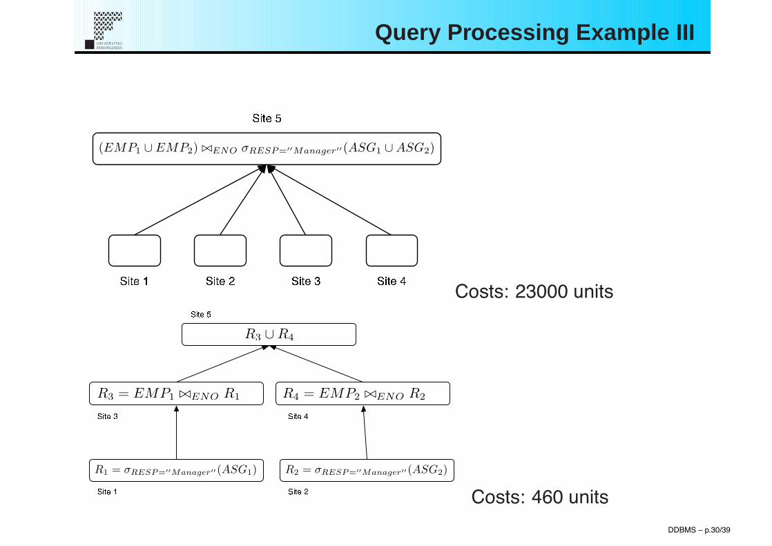
2 equivalent distributed execution strategies are considered. The costs foreach strategy is computed using a total-cost function:
1 tuple acces = 1 unit1 tuple transfer = 10 units
DDBMS – p.29/39

Query Processing Example III
(EMP1 ! EMP2) !"ENO #RESP=!!Manager!!(ASG1 ! ASG2)
DDBMS – p.30/39

Query Processing Example III
(EMP1 ! EMP2) !"ENO #RESP=!!Manager!!(ASG1 ! ASG2)
R1 = !RESP=!!Manager!!(ASG1) R2 = !RESP=!!Manager!!(ASG2)
R3 = EMP1 !"ENO R1 R4 = EMP2 !"ENO R2
R3 ! R4
DDBMS – p.30/39
Query Processing Example III
(EMP1 ! EMP2) !"ENO #RESP=!!Manager!!(ASG1 ! ASG2)
Costs: 23000 units
R1 = !RESP=!!Manager!!(ASG1) R2 = !RESP=!!Manager!!(ASG2)
R3 = EMP1 !"ENO R1 R4 = EMP2 !"ENO R2
R3 ! R4
Costs: 460 unitsDDBMS – p.30/39
Query Processing Architecture
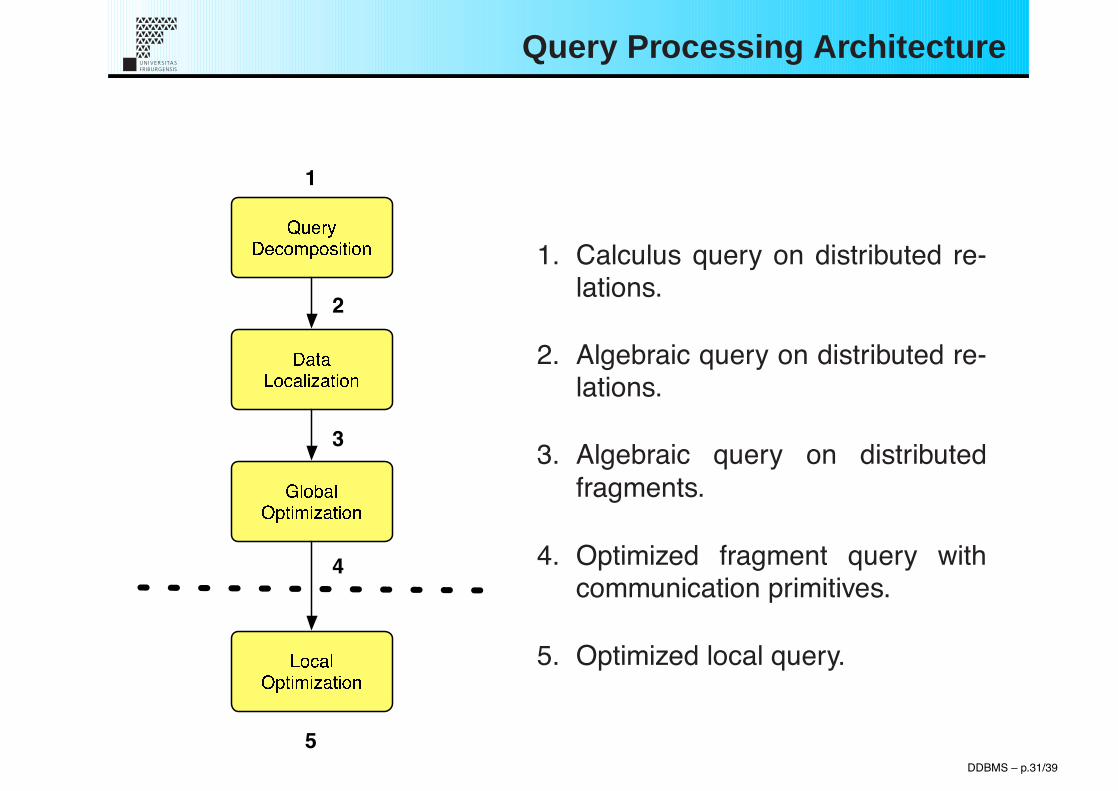
1. Calculus query on distributed re-lations.
2. Algebraic query on distributed re-lations.
3. Algebraic query on distributedfragments.
4. Optimized fragment query withcommunication primitives.
5. Optimized local query.
DDBMS – p.31/39

Query Decomposition I
Validates sematics (ex. types of operations, existance of relations, ...)
Transforms WHERE-clause to CNF.
Eliminates redundancy in WHERE-clause (logical idempotency rules).
Construction of operator tree.
Optimizes operator tree by applying transformation rules.
Rewrites operator tree in relation algebra.
DDBMS – p.32/39
Query Decomposition II
!"ENO
EMPASG
PROJ
!"PNO
!ENAME != !!Mueller!!
!PNAME =!!CAD!!
!DUR = 12 ! DUR = 24
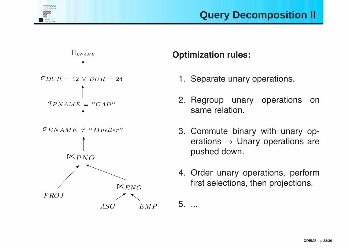
!ENAME Optimization rules:
1. Separate unary operations.
2. Regroup unary operations onsame relation.
3. Commute binary with unary op-erations ! Unary operations arepushed down.
4. Order unary operations, performfirst selections, then projections.
5. ...
DDBMS – p.33/39

Data Localization
Adds distribution to query.
Transforms algebraic query on global relations to algebraic query onphysical fragments.
Applies fragment reconstruction rules (( or "!) to query.
Eliminates selections / projections if they contradict fragmentpredicats.
DDBMS – p.34/39
Global Optimization I
After data localization, the global query can be executed by addingcommunication primitives in a systematic way. But the ordering of theseprimitives again creates many equivalent strategies.
DDBMS – p.35/39

Global Optimization I
After data localization, the global query can be executed by addingcommunication primitives in a systematic way. But the ordering of theseprimitives again creates many equivalent strategies.
The problem of finding a good strategy is so difficult that in most cases, alleffort is concentrated rather on avoiding bad strategies that on finding agood one.
Again, the heuristics are all based on cost-functions which use databasestatistics. Because this optimization step concerns communicationprimitives, communication cost is a central point.
Expressing the costs to transmit relation R from site S1 to site S2:
size(R) = card(R) + length(R)
where length(R) is the length (in bytes) of a single tuple.
DDBMS – p.35/39
Global Optimization II
Optimization in 3 steps:
1. Build search space (all possible execution strategies represented asoperator trees) # O(n!) for n relations.
2. Apply cost function to each QEP = Query Execution Plan3. Choose the best !
DDBMS – p.36/39

Global Optimization II
Optimization in 3 steps:
1. Build search space (all possible execution strategies represented asoperator trees) # O(n!) for n relations.
2. Apply cost function to each QEP = Query Execution Plan3. Choose the best !
Carthesian products and joins have most influence on total costs. !Optimization is concentrated on join trees = operator trees whose nodesare joins or Carthesian products.
Building the search space:dynamic programming: builds all possible plans. Partial plans whichare not likely to lead to a good plan are pruned.randomized strategies: apply dynamic prog. to obtain”not-so-bad-solution” and investigate neighboring trees (byexchanging relations).
DDBMS – p.36/39

Global Optimization III
The join tree shape is a useful indicator: linear trees! no parallelism,bushy trees! full parallelism.
Discussing the cost functions goes beyond the scope of this presentation(case studies)...
DDBMS – p.37/39

Local Optimization
After global optimization, each sub-query is delegated to the appropriatesite (due to the communication primitives). Clearly, all sites canthemselves optimize their local queries according to their additionalknowledge about their data.
This is local optimization ...
DDBMS – p.38/39
Discussion
Questions ?
DDBMS – p.39/39
Copyright © 2022 FDOKUMEN