Structured Robust Submodular Maximization - arXiv

arX

iv:1

710.

0474

0v3

[cs

.DS]

13

Oct

202

0

Structured Robust Submodular Maximization:Offline and Online Algorithms

Alfredo Torrico* Mohit Singh† Sebastian Pokutta‡

Nika Haghtalab§ Joseph (Seffi) Naor¶ Nima Anari||

Abstract

Constrained submodular function maximization has been used in subset selection problemssuch as selection of most informative sensor locations. While these models have been quitepopular, the solutions Constrained submodular function maximization has been used in subsetselection problems such as selection of most informative sensor locations. While these modelshave been quite popular, the solutions obtained via this approach are unstable to perturbations indata defining the submodular functions. Robust submodular maximization has been proposed asa richer model that aims to overcome this discrepancy as well as increase the modeling scope ofsubmodular optimization.

In this work, we consider robust submodular maximization with structured combinatorialconstraints and give efficient algorithms with provable guarantees. Our approach is applicableto constraints defined by single or multiple matroids, knapsack as well as distributionally robustcriteria. We consider both the offline setting where the data defining the problem is known inadvance as well as the online setting where the input data is revealed over time. For the offlinesetting, we give a general (nearly) optimal bi-criteria approximation algorithm that relies on newextensions of classical algorithms for submodular maximization. For the online version of theproblem, we give an algorithm that returns a bi-criteria solution with sub-linear regret.

1 Introduction

Constrained submodular function maximization has seen significant progress in recent years in the de-sign and analysis of new algorithms with guarantees (Calinescu et al., 2011; Ene and Nguyen, 2016;Buchbinder and Feldman, 2016; Sviridenko, 2004), as well as numerous applications - especially inconstrained subset selection problems (Powers et al., 2016a; Lin and Bilmes, 2009; Krause and Guestrin,2005a; Krause et al., 2009, 2008a,b) and more broadly machine learning. A typical example is theproblem of picking a subset of candidate sensor locations for spatial monitoring of certain phenom-ena such as temperature, ph values, humidity, etc. (Krause et al., 2008a). Here the goal is typically tofind sensor locations that achieve the most coverage or give the most information about the observedphenomena. Submodularity naturally captures the decreasing marginal gain in the coverage, or the in-formation acquired about relevant phenomena by using more sensors (Das and Kempe, 2008). While

*Polytechnique Montréal, Canada. Email: [email protected]†Georgia Institute of Technology, Atlanta. Email: [email protected]‡ZIB, TU Berlin. Email: [email protected]§Cornell University, Email: [email protected]¶Technion, Haifa, Israel. Email: [email protected]||Stanford University, Stanford. Email: [email protected]

1

http://arxiv.org/abs/1710.04740v3

submodular optimization offers an attractive model for such scenarios, there are a few key shortcom-ings, which motivated robust submodular optimization in the cardinality case (Krause et al., 2008a),so as to optimize against several functions simultaneously:

1. The sensors are typically used to measure various parameters at the same time. Observationsfor these parameters need to be modeled via different submodular functions.

2. Many of the phenomena being observed are non-stationary and highly variable in certain loca-tions. To obtain a good solution, a common approach is to use different submodular functionsto model different spatial regions.

3. The submodular functions are typically defined using data obtained from observations, andimprecise information can lead to unstable optimization problems. Thus, there is a desire tocompute solutions that are robust to perturbations of the submodular functions.

Given the computational complexity of optimizing several functions simultaneously, Krause et al.(2008a) motivated a bicriteria approach. In simple words, in order to obtain provable guarantees, oneneeds to trade off the quality of the solution measured by its objective value with the “size” of thesolution. In the case of a single cardinality constraint, Krause et al. (2008a) proposes a natural relax-ation which consists in allowing more elements in the final set, i.e., violating the feasibility constraint.However, to obtain provable guarantees for more general combinatorial constraints relaxing the sizeof feasible sets is not enough.

Our main contribution is the development of new algorithms with provable guarantees for robustsubmodular optimization under a large class of combinatorial constraints. These include partitionconstraints, where local cardinality constraints are placed on disjoint parts of the ground set. Moregenerally, we consider matroid and knapsack constraints.

We provide bi-criteria approximations that trade-off the approximation factor with the “size” ofthe solution, measured by the number ℓ of feasible sets {Si}i∈[ℓ] whose union constitutes the finalsolution S. While this might be nonintuitive at first, it turns out that the union of feasible sets corre-sponds to an appropriate analog of the single cardinality constraint. Some special cases of interestare:

1. Partition constraints. Given a partition of the candidate sensor locations, the feasible setscorrespond to subsets that satisfy a cardinality constraint on each part of the partition. Theunion of feasible sets here corresponds to relaxing the cardinality constraints separately foreach part. This results in a stronger guarantee than relaxing the constraint globally as would bethe case in the single cardinality constraint case.

2. Gammoid. Given a directed graph and a subset of nodes T , the feasible sets correspond tosubsets S that can reach T via disjoint paths in the graph. Gammoids appear in flow basedmodels, for example in reliable routing. The union of feasible sets now corresponds to sets Sthat can reach T via paths such that each vertex appears in few paths.

We consider both offline and online versions of the problem, where the data is either known a-priori or is revealed over time, respectively. For the offline version of the problem, we provide ageneral procedure that iteratively utilizes any standard algorithm for submodular maximization toproduce a solution which is a union of multiple feasible sets. The analysis relies on known insightsabout the performance of the classical greedy algorithm when is used for cardinality constraint. Forthe online case, we introduce new technical ingredients that might be broadly applicable in onlinerobust optimization. Our work significantly expands on previous works on robust submodular opti-

2

mization that focused on a single cardinality constraint (Krause et al., 2008a). Moreover, our worksubstantially differ from its proceeding version (Anari et al., 2019), because: (1) we provide a generaland flexible framework to design an offline bi-criteria algorithm; (2) we give significant implementa-tion improvements and support our theoretical results via an exhaustive computational study on tworeal-world applications.

1.1 Problem Formulation

As we describe below, we study offline and online variations of robust submodular maximization

under structured combinatorial constraints. While our results holds for more general constraints,we focus our attention first on matroid constraints that generalize the partition as well as the gam-moid structural constraints mentioned above. We discuss extensions to other class of constraints inSection 4.

Consider a non-negative set function f : 2V → R+. We denote the marginal value for any subsetA ⊆ V and e ∈ V by fA(e) := f(A+e)−f(A), where A+e := A∪{e}. Function f is submodular ifand only if it satisfies the diminishing returns property. Namely, for any e ∈ V and A ⊆ B ⊆ V \{e},fA(e) ≥ fB(e). We say that f is monotone if for any A ⊆ B ⊆ V , we have f(A) ≤ f(B). Most ofour results are concerned with optimization of monotone submodular functions.

A natural class of constraints considered in submodular optimization are matroid constraints. Fora ground set V and a family of sets I ⊆ 2V , M = (V,I) is a matroid if (1) for all A ⊂ B ⊆ V ,if B ∈ I then A ∈ I and (2) for all A,B ∈ I with |A| < |B|, there is e ∈ B \ A such thatA ∪ {e} ∈ I . Sets in such a family I are called independent sets, or simply put, feasible sets for thepurpose of optimization. Maximal independent sets are called basis. Finally, the rank of a matroid isthe maximum size of an independent set in the matroid.

The classical problem of maximizing a single monotone submodular function f : 2V → R+

under a matroid constraintM = (V,I) is formally stated as: maxA∈I f(A). Throughout this paper,we say that a polynomial time algorithmA achieves a (1−β) approximation factor for this problem, ifit returns a feasible solution S ∈ I such that f(S) ≥ (1−β) ·maxA∈I f(A). WhenA is randomized,we say that A achieves a (1−β)-approximation in expectation if E[f(S)] ≥ (1− β) ·maxA∈I f(A).The well-known standard greedy algorithm (Nemhauser et al., 1978) is an example ofAwith β = 1/2(Fisher et al., 1978). We will denote by time(A) the running time of A.

In this work, we consider the robust variation of the above submodular maximization problem.That is, for a matroid M = (V,I), and a given collection of k monotone submodular functionsfi : 2

V → R+ for i ∈ [k], our goal is to efficiently select a set S that maximizes mini∈[k] fi(S). Wedefine a (1− ǫ)-approximately optimal solution S as

mini∈[k]

fi(S) ≥ (1− ǫ) ·maxA∈I

mini∈[k]

fi(A). (1)

We also consider the online variation of the above optimization problem in presence of an adver-sary. In this setting, we are given a fixed matroidM = (V,I). At each time step t ∈ [T ], we choosea set St. An adversary then selects a collection of k monotone submodular functions {f t

i }i∈[k] :

2V → [0, 1]. We receive a reward of mini∈[k] E[fti (S

t)], where the expectation is taken over anyrandomness in choosing St. We can then use the knowledge of the adversary’s actions, i.e., oracleaccess to {f t

i }i∈[k], in our future decisions. We consider non-adaptive adversaries whose choices{f t

i }i∈[k] are independent of Sτ for τ < t. In other words, an adversarial sequence of functions{f1

i }i∈[k], . . . , {fTi }i∈[k] is chosen upfront without being revealed to the optimization algorithm. Our

goal is to design an algorithm that maximizes the total payoff∑

t∈[T ]mini∈[k] E[fti (S

t)]. Thus, we

3

would like to obtain a cumulative reward that competes with that of the fixed set S ∈ I we should haveplayed had we known all the functions f t

i in advance, i.e., compete with maxS∈I∑

t∈[T ]mini∈[k] fti (S).

As in the offline optimization problem, we also consider competing with (1− ǫ) fraction of the abovebenchmark. In this case, Regret1−ǫ(T ) denotes how far we are from this goal. That is,

Regret1−ǫ(T ) = (1− ǫ) ·maxS∈I

∑

t∈[T ]

mini∈[k]

f ti (S)−

∑

t∈[T ]

mini∈[k]

E[

f ti (S

t)]

. (2)

We desire algorithms whose (1 − ǫ)-regret is sublinear in T . That is, we get arbitrarily close to a(1− ǫ) fraction of the benchmark as T →∞.

The offline (Equation 1), or online (Equation 2) variations of robust monotone submodular func-tions, are known to be NP-hard to approximate to any polynomial factor when the algorithm’s choicesare restricted to the family of independent sets I (Krause et al., 2008a). Therefore, to obtain anyreasonable approximation guarantee we need to relax the algorithm’s constraint set. Such an approx-imation approach is called a bi-criteria approximation scheme in which the algorithm outputs a setwith a nearly optimal objective value, while ensuring that the set used is the union of only a few inde-

pendent sets in I . More formally, to get a (1 − ǫ)-approximate solutions, we may use a set S whereS = S1 ∪ · · · ∪ Sℓ such that S1, . . . , Sℓ ∈ I and ℓ is a function of 1

ǫ and other parameters. Since theoutput set S is possibly infeasible, we define the violation ratio ν as the minimum number of feasiblesets whose union is S. To exemplify this, consider partition constraints: here we are given a partition{P1, . . . , Pq} of the ground set and the goal is to pick a subset that includes at most bj elements frompart Pj for each j. Then, the union of ℓ feasible sets have at most ℓ · bj elements in each part. In ourexample, the violation ratio corresponds to ν = maxj∈[q]⌈|S ∩ Pj |/bj⌉.1.2 Our Results and Contributions

We present (nearly tight) bi-criteria approximation algorithms for the offline and online variationsof robust monotone submodular optimization under matroid constraints. Throughout the paper, weassume that the matroid is accessible via an independence oracle and the submodular functions areaccessible via a value oracle. Moreover, we use loga to denote logarithm with base a (when thesubscript is not explicit we assume is base 2, i.e, log := log2) and ln to denote the natural logarithm.

For the offline setting of the problem we obtain the following general result:

Theorem 1. Consider a polynomial time (1 − β)-approximation algorithm A for the problem of

maximizing a single monotone submodular function subject to a matroid constraint. Then, for the

offline robust submodular optimization problem (1), for any 0 < ǫ < 1, there is a polynomial time

bicriteria algorithm that uses ext-A as a subroutine, runs in

O

(

time(A) · log1/β(

k

ǫ

)

· log(n) ·min

{

nk

ǫ, log1+ǫ(max

e,jfj(e))

})

time and returns a set SALG, such that

E

[

mini∈[k]

fi(SALG)

]

≥ (1− ǫ) ·maxS∈I

minj∈[k]

fj(S),

where the expectation is taken over any randomization of A, SALG = S1 ∪ · · · ∪ Sℓ with ℓ =⌈log1/β k

ǫ ⌉, and S1, . . . , Sℓ ∈ I .

4

The subroutine ext-A that achieves this result is an extended version of the algorithm A. SinceA outputs a feasible set, then ext-A reuses A in an iterative scheme, so that it generates a small

family of feasible sets whose union achieves the (1 − ǫ)-guarantee. The argument is reminiscent ofa well-known fact for submodular function maximization under cardinality constraints: letting thestandard greedy run longer results in better approximations at the expense of violating the cardinalityconstraint. Our extended algorithm ext-A works in a similar spirit, however it iteratively producesfeasible sets in the matroid. This framework generalizes the idea presented in (Anari et al., 2019).We emphasize that our procedure does not correspond to an extension of the algorithm for cardinalityconstraint presented in (Krause et al., 2008a). The natural extension of their algorithm to a singlematroid constraint would be to run an algorithm A over a larger feasibility constraint. However, thisapproach does not provide any bicriteria approximation. The main challenge for matroid constraintsis to define an appropriate notion of violation. In our work, we measure violation by the number ofindependent sets that are needed to cover the given set, as a contrast of Krause et al. (2008a) whodefine it in terms of cardinality. Our subroutine ext-A constructs a family of independent sets andthat is pivotal to obtain provable guarantees.

A natural candidate for A is the standard greedy algorithm, from now on referred as Greedy.Since Greedy achieves a 1/2 approximation factor (Fisher et al., 1978), then the number of feasiblesets needed is ℓ = ⌈log2 k

ǫ ⌉ (Anari et al., 2019). Unfortunately, Greedy’s running time O(n · r)depends on the rank of the matroid r. This can be computationally inefficient when r is sufficientlylarge. To improve this, in Section 2.1 we propose an extended version of the threshold greedy algo-rithm introduced by Badanidiyuru and Vondrák (2014). The main advantage of the threshold greedyalgorithm, further referred as ThGreedy, is its running time which does not depend on the rank ofthe matroid. Formally, we obtain the following corollary.

Corollary 1. For the offline robust submodular optimization problem (1), for any 0 < ǫ, δ < 1, there

is a polynomial time bicriteria algorithm that uses ext-ThGreedy as a subroutine, runs in

O

(

n

δ· log

(n

δ

)

· log2(

k

ǫ

)

· log(n) ·min

{

nk

ǫ, log1+ǫ(max

e,jfj(e))

})

time and returns a set SALG such that

mini∈[k]

fi(SALG) ≥ (1− ǫ) ·max

S∈Iminj∈[k]

fj(S),

where SALG = S1 ∪ · · · ∪ Sℓ with ℓ = ⌈log2 kǫ ⌉, and S1, . . . , Sℓ ∈ I .

To achieve a tight bound on the size of the family ℓ, we use an improved version of the contin-uous greedy algorithm (Vondrák, 2008; Badanidiyuru and Vondrák, 2014) as the inner algorithm A.Since the continuous greedy algorithm achieves a 1 − 1/e approximation ratio, we need ℓ = ⌈ln k

ǫ ⌉feasible sets to achieve a 1 − ǫ fraction of the true optimum, which matches the hardness result pre-sented in (Krause et al., 2008a). This bi-criteria algorithm is much simpler than the one presented in(Anari et al., 2019). We present the main offline results and the corresponding proofs in Section 2.

One might hope that similar results can be obtained even when functions are non-monotone (butstill submodular). As we show in Section 2.2 this is not possible. To support our theoretical guaran-tees we provide an exhaustive computational study in Section 2.3. In this part, we observe that themain computational bottleneck of the bi-criteria algorithms is to certify near-optimality of the outputsolution. To solve this, we present significant implementation improvements such as lazy evaluations

5

and an early stopping criterion, which empirically show how the computational cost can be drasticallyimproved.

Our offline approach is quite flexible in the sense that Theorem 1 uses an arbitrary algorithm A.This allows us to consider different algorithms in the literature of submodular optimization and furtherextend our results to other classes of constraints, such as knapsack constraints or multiple matroids.We describe these extensions in Section 4.

A natural question is whether our algorithm can be carried over into the online setting, wherefunctions are revealed over time. For the online variant, we present the following result:

Theorem 2. For the online robust submodular optimization problem (2), for any 0 < ǫ < 1, there is

a randomized polynomial time algorithm that returns a set St for each stage t ∈ [T ], we get

∑

t∈[T ]

mini∈[k]

E[

f ti (S

t)]

≥ (1− ǫ) ·maxS∈I

∑

t∈[T ]

mini∈[k]

f ti (S)−O

(

(1− ǫ)n5

4

√T)

,

where St = St1 ∪ · · · ∪ St

ℓ with ℓ = ⌈ln 1ǫ ⌉, and St

1, . . . , Stℓ ∈ I .

We remark that the guarantee of Theorem 2 holds with respect to the minimum of E[f ti (S

t)],as opposed to the guarantee of Theorem 1 that directly bounds the minimum of fi(S). Therefore,the solution for the online algorithm is a union of only ⌈ln 1

ǫ ⌉ independent sets, in contrast to theoffline solution which is the union of ⌈log k

ǫ ⌉ independent sets. The main challenge in the onlinealgorithm is to deal with non-convexity and non-smoothness due to submodularity exacerbated bythe robustness criteria. Our approach to coping with the robustness criteria is to use the soft-min

function − 1α ln

∑

i∈[k] e−αgi , defined for a collection of smooth functions {gi}i∈[k] and a suitable

parameter α > 0. This function is also known as log-sum-exp; for some of its properties and ap-plications we refer the interested reader to (Calafiore and El Ghaoui, 2014). While the choice of thespecific soft-min function is seemingly arbitrary, one feature is crucial for us: its gradient is a con-vex combination of the gradients of the gi’s. Using this observation, we use parallel instances ofthe Follow-the-Perturbed-Leader (FPL) algorithm, presented by Kalai and Vempala (2005), one foreach discretization step in the continuous greedy algorithm. We believe that the algorithm might beof independent interest to perform online learning over a minimum of several functions, a commonfeature in robust optimization. The main result and a its proof appears in Section 3.

1.3 Related Work

Building on the classical work of Nemhauser et al. (1978), constrained submodular maximizationproblems have seen much progress recently (see for example (Calinescu et al., 2011; Chekuri et al.,2010; Buchbinder et al., 2014, 2016)). Robust submodular maximization generalizes submodularfunction maximization under a matroid constraint for which a (1−1

e )-approximation is known (Calinescu et al.,2011) and is optimal. The problem has been studied for constant k by Chekuri et al. (2010) who give

a (1 − 1e − ǫ)-approximation algorithm with running time O

(

nkǫ

)

. Closely related to our problem

is the submodular cover problem where we are given a submodular function f , a target b ∈ R+,and the goal is to find a set S of minimum cardinality such that f(S) ≥ b. A simple reductionshows that robust submodular maximization under a cardinality constraint reduces to the submod-ular cover problem (Krause et al., 2008a). Wolsey (1982) showed that the greedy algorithm givesan O(ln n

ǫ )-approximation, where the output set S satisfies f(S) ≥ (1 − ǫ)b. Krause et al. (2008a)use this approximation to build a bi-criteria algorithm for the cardinality case which achieves tight

6

bounds. This approach falls short of achieving a bi-criteria approximation when the problem is de-fined over a matroid. A natural extension of their approach to matroid constraints would be to runa single algorithm A over a larger feasibility constraint. However, this procedure does not provideany guarantee. Therefore, the main challenge is to define an appropriate notion of violation. In thiswork, we measure violation not by cardinality, as in (Krause et al., 2008a), but by the number of in-dependent sets that are needed to cover the given set. Our subroutine ext-A picks one feasible setat a time and that is crucial to obtain provable guarantees. Powers et al. (2016b) considers the samerobust problem with matroid constraints. However, they take a different approach by presenting abi-criteria algorithm that outputs a feasible set that is good only for a fraction of the k monotone sub-modular functions. A deletion-robust submodular optimization model is presented in (Krause et al.,2008a), which is later studied by Orlin et al. (2016); Bogunovic et al. (2017); Kazemi et al. (2018).Influence maximization (Kempe et al., 2003) in a network has been a successful application of sub-modular maximization and recently, He and Kempe (2016) and Chen et al. (2016) study the robustinfluence maximization problem. Robust optimization for non-convex objectives (including submod-ular functions) has been also considered by Chen et al. (2017), however with weaker guarantees thanours due to the extended generality. Specifically, their algorithm outputs r log k

ǫ2 OPTfeasible sets whose

union achieves a factor of (1 − 1/e − ǫ). Finally, Wilder (2017) studies a similar problem in whichthe set of feasible solutions is the set of all distributions over independent sets of a matroid. In partic-ular, for our setting Wilder (2017) gives an algorithm that outputs O( log kǫ3 ) feasible sets whose unionobtains (1 − 1/e)2 fraction of the optimal solution. Our results are stronger than the ones obtainedby Chen et al. (2017) and Wilder (2017), since we provide the same guarantees using the union offewer feasible sets. Other variants of the robust submodular maximization problem are studied byMitrovic et al. (2018); Staib et al. (2018).

There has been some prior work on online submodular function maximization that we briefly re-view here. Streeter and Golovin (2008) study the budgeted maximum submodular coverage problemand consider several feedback cases (denote B a integral bound for the budget): in the full informa-tion case, a (1 − 1

e )-expected regret of O(√BT lnn) is achieved, but the algorithm uses B experts

which may be very large. In a follow-up work, Golovin et al. (2014) study the online submodularmaximization problem under partition constraints, and then they generalize it to general matroid con-straints. For the latter one, the authors present an online version of the continuous greedy algorithm,which relies on the Follow-the-Perturbed-Leader algorithm of Kalai and Vempala (2005) and obtain a(1− 1

e )-expected regret of O(√T ). Similar to this approach, our bi-criteria online algorithm will also

use the Follow-the-Perturbed-Leader algorithm as a subroutine. Recent results on other variants ofthe online submodular maximization problem are studied in (Soma, 2019) and (Zhang et al., 2019).

2 The Offline Case

In this section, we consider offline robust optimization (Equation 1) under matroid constraints.

2.1 General Offline Algorithm and Analysis

In this section, we present a general procedure to achieve a (nearly) tight bi-criteria approximationfor the problem of interest and prove Theorem 1.

First, consider a non-negative monotone submodular function g : 2V → R+, a matroid M =(V,I), and a polynomial time (1 − β)-approximation algorithm A for the problem of maximizingg over M. Formally, in the deterministic case, A outputs a feasible set S ∈ I such that g(S) ≥(1 − β) · maxA∈I g(A). If g(∅) 6= 0, then we define a new function g′ : 2V → R+ as g′(A) :=g(A) − g(∅), which remains being monotone and submodular. The approximation guarantee in this

7

case is g(S)− g(∅) ≥ (1− β) ·maxA∈I{g(A)− g(∅)}. When A is a randomized algorithm, we saythat A achieves a (1 − β) factor in expectation, if A outputs a random feasible set S ∈ I such thatE[g(S) − g(∅)] ≥ (1 − β) · maxA∈I{g(A) − g(∅)}. We define in Algorithm 1 our main procedureext-A as an extended version of A that runs iteratively ℓ ≥ 1 times.

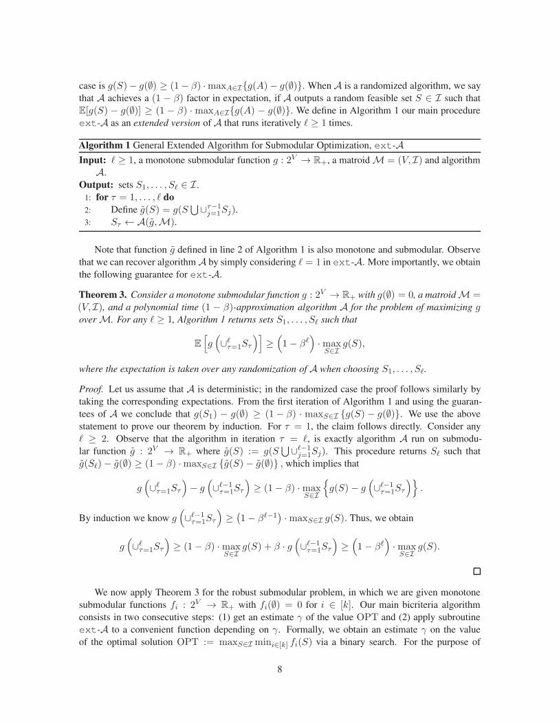
Algorithm 1 General Extended Algorithm for Submodular Optimization, ext-AInput: ℓ ≥ 1, a monotone submodular function g : 2V → R+, a matroidM = (V,I) and algorithmA.

Output: sets S1, . . . , Sℓ ∈ I .1: for τ = 1, . . . , ℓ do

2: Define g̃(S) = g(S⋃∪τ−1

j=1Sj).3: Sτ ← A(g̃,M).

Note that function g̃ defined in line 2 of Algorithm 1 is also monotone and submodular. Observethat we can recover algorithm A by simply considering ℓ = 1 in ext-A. More importantly, we obtainthe following guarantee for ext-A.

Theorem 3. Consider a monotone submodular function g : 2V → R+ with g(∅) = 0, a matroidM =(V,I), and a polynomial time (1 − β)-approximation algorithm A for the problem of maximizing goverM. For any ℓ ≥ 1, Algorithm 1 returns sets S1, . . . , Sℓ such that

E

[

g(

∪ℓτ=1Sτ

)]

≥(

1− βℓ)

·maxS∈I

g(S),

where the expectation is taken over any randomization of A when choosing S1, . . . , Sℓ.

Proof. Let us assume that A is deterministic; in the randomized case the proof follows similarly bytaking the corresponding expectations. From the first iteration of Algorithm 1 and using the guaran-tees of A we conclude that g(S1) − g(∅) ≥ (1− β) · maxS∈I {g(S) − g(∅)}. We use the abovestatement to prove our theorem by induction. For τ = 1, the claim follows directly. Consider anyℓ ≥ 2. Observe that the algorithm in iteration τ = ℓ, is exactly algorithm A run on submodu-lar function g̃ : 2V → R+ where g̃(S) := g(S

⋃∪ℓ−1j=1Sj). This procedure returns Sℓ such that

g̃(Sℓ)− g̃(∅) ≥ (1− β) ·maxS∈I {g̃(S)− g̃(∅)} , which implies that

g(

∪ℓτ=1Sτ

)

− g(

∪ℓ−1τ=1Sτ

)

≥ (1− β) ·maxS∈I

{

g(S)− g(

∪ℓ−1τ=1Sτ

)}

.

By induction we know g(

∪ℓ−1τ=1Sτ

)

≥(

1− βℓ−1)

·maxS∈I g(S). Thus, we obtain

g(

∪ℓτ=1Sτ

)

≥ (1− β) ·maxS∈I

g(S) + β · g(

∪ℓ−1τ=1Sτ

)

≥(

1− βℓ)

·maxS∈I

g(S).

We now apply Theorem 3 for the robust submodular problem, in which we are given monotonesubmodular functions fi : 2V → R+ with fi(∅) = 0 for i ∈ [k]. Our main bicriteria algorithmconsists in two consecutive steps: (1) get an estimate γ of the value OPT and (2) apply subroutineext-A to a convenient function depending on γ. Formally, we obtain an estimate γ on the valueof the optimal solution OPT := maxS∈I mini∈[k] fi(S) via a binary search. For the purpose of

8

the proof of Theorem 1, given parameter ǫ > 0, let us assume that γ has relative error 1 − ǫ2 , i.e.,

(

1− ǫ2

)

OPT ≤ γ ≤ OPT . As in (Krause et al., 2008a), let g : 2V → R+ be defined for any S ⊆ Vas follows

g(S) :=1

k

∑

i∈[k]

min{fi(S), γ}. (3)

Observe that maxS∈I g(S) = γ whenever γ ≤ OPT. Moreover, note that g is also a monotonesubmodular function. Therefore, the second step of the bicriteria algorithm is to run algorithm ext-A on the function g to obtain a candidate solution. A more detailed description of the algorithm canbe found in Section 2.3.

Proof of Theorem 1. We assume A to be deterministic; the randomized case can be easily provedby consider the proof below for each realization sequence of S1, . . . , Sℓ. Consider the family ofmonotone submodular functions {fi}i∈[k] and define g as in equation (3) using parameter γ withrelative error of 1 − ǫ

2 . If we run Algorithm 1 on g with ℓ ≥ ⌈log1/β 2kǫ ⌉, we get a set SALG =

S1 ∪ · · · ∪ Sℓ, where Sj ∈ I for all j ∈ [ℓ]. Moreover, Theorem 3 implies that

g(SALG) ≥(

1− βℓ)

·maxS∈I

g(S) ≥(

1− ǫ

2k

)

· γ.

Now, we will prove that fi(SALG) ≥(

1− ǫ2

)

· γ, for all i ∈ [k]. Assume by contradiction that thereexists an index i∗ ∈ [k] such that fi∗(SALG) <

(

1− ǫ2

)

·γ. Since, we know that min{fi(SALG), γ} ≤γ for all i ∈ [k], then

g(SALG) ≤ 1

k· fi∗(SALG) +

k − 1

k· γ <

1− ǫ/2

k· γ +

k − 1

k· γ =

(

1− ǫ

2k

)

· γ,

contradicting g(SALG) ≥(

1− ǫ2k

)

·γ. Therefore, we obtain fi(SALG) ≥

(

1− ǫ2

)

·γ ≥ (1−ǫ)·OPT,for all i ∈ [k] as claimed.

Running time analysis. In this section, we study the running time of the bi-criteria algorithm wejust presented. To show that a set of polynomial size of values for γ exists such that one of themsatisfies (1 − ǫ/2)OPT ≤ γ ≤ OPT, we simply try γ = nfi(e)(1 − ǫ/2)j for all i ∈ [k], e ∈ V ,and j = 0, . . . , ⌈ln1−ǫ/2(1/n)⌉. Note that there exists an index i∗ ∈ [k] and a set S∗ ∈ I such thatOPT = fi∗(S

∗). Now let e∗ = argmaxe∈S∗ fi∗(e). Because of submodularity and monotonicity wehave 1

|S∗|fi∗(S∗) ≤ fi∗(e

∗) ≤ fi∗(S∗). So, we can conclude that 1 ≥ OPT /nfi∗(e

∗) ≥ 1/n, whichimplies that j = ⌈ln1−ǫ/2(OPT /nfi∗(e

∗))⌉ is in the correct interval, obtaining

(1− ǫ/2)OPT ≤ nfi∗(e∗)(1− ǫ/2)j ≤ OPT .

We remark that the dependency of the running time on ǫ can be made logarithmic by running abinary search on j as opposed to trying all j = 0, . . . , ⌈ln1−ǫ/2(1/n)⌉. This would take at mostnkǫ · log n iterations. We could also say that doing a binary search to get a value up to a relative error

of 1 − ǫ/2 of OPT would take log1+ǫOPT. So, we consider the minimum of those two quantitiesmin{nkǫ · log n, log1+ǫOPT}. Given that Algorithm 1 runs in ℓ · time(A) where ℓ = ⌈log1/β k

ǫ ⌉ is the

number of rounds, we conclude that the bi-criteria algorithm runs in O(time(A) · log1/β kǫ ·min{nkǫ ·

log n, log1+ǫOPT}) time.

9

2.1.1 Two Deterministic Classical Algorithms: Greedy and Local Search.

The most natural candidate for A is Greedy (Nemhauser et al., 1978) which achieves a ratio of 1/2for the problem of maximizing a single monotone submodular function subject to a matroid constraint(Fisher et al., 1978). In this case, we know that time(Greedy) = O(n · r), where r is the rank ofthe matroid. Using Greedy, we are able to design its extended version ext-Greedy, formallyoutlined in Algorithm 2.

Algorithm 2 Extended Greedy Algorithm for Submodular Optimization, ext-Greedy

Input: ℓ ≥ 1, monotone submodular function g : 2V → R+, matroidM = (V,I).Output: sets S1, . . . , Sℓ ∈ I .

1: for τ = 1, . . . , ℓ do

2: Sτ ← ∅3: while Sτ is not a basis ofM do

4: Compute e∗ = argmaxSτ+e∈I{g(∪τj=1Sj + e)}.5: Update Sτ ← Sτ + e∗.

From Theorem 1 we can easily derive the following corollary for ext-Greedy:

Corollary 2. For the offline robust submodular optimization problem (1), for any 0 < ǫ, δ < 1, there

is a polynomial time bicriteria algorithm that uses ext-Greedy as a subroutine, runs in

O

(

n · r · log2(

k

ǫ

)

· log(n) ·min

{

nk

ǫ, log1+ǫ(max

e,jfj(e))

})


mini∈[k]


S∈Iminj∈[k]

fj(S),

where SALG = S1 ∪ · · · ∪ Sℓ with ℓ = ⌈log2 kǫ ⌉, and S1, . . . , Sℓ ∈ I .

Another natural candidate is the standard local search algorithm, from now on referred as LS(Fisher et al., 1978). Roughly speaking, this algorithm starts with a maximal feasible set and itera-tively swap elements if the objective is improved while maintaining feasibility. If the objective can-not be longer improved, then the algorithm stops. Fisher et al. (1978) prove that this procedure alsoachieves a 1/2-approximation, i.e., β = 1/2. However, the running time of LS cannot be explicitlyobtained. Finally, for the offline robust problem the extended version of the local search algorithm,ext-LS, achieves the same guarantees than ext-Greedy, but without an explicit running time.

2.1.2 Improving Running Time: Extended Threshold Greedy.

As we mentioned earlier, we are interested in designing efficient bi-criteria algorithms for the robustsubmodular problem (1). Unfortunately, the subroutine ext-Greedy performs O(n·r ·log2 k

ǫ ) func-tion calls, which can be considerably inefficient when r is sufficiently large. Our objective in this sec-tion is to study a variant of the standard greedy algorithm that perform less function calls and whoserunning time does not depend on the rank of the matroid. For our purposes, we consider the thresh-

old greedy algorithm, from now on referred as ThGreedy, introduced by Badanidiyuru and Vondrák(2014). Roughly speaking, this procedure iteratively adds elements whose marginal value is abovecertain threshold while maintaining feasibility. Unlike Greedy, ThGreedymay add more than one

10

element in a single iteration. For cardinality constraint, Badanidiyuru and Vondrák (2014) show thatthe threshold greedy algorithm achieves a (1−1/e−δ)-approximation factor, where δ is the parameterthat controls the threshold. Moreover, time(ThGreedy) = O(nδ log

nδ ), which does not depend on

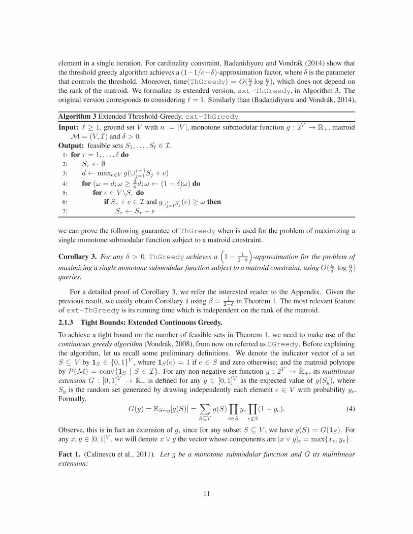
the rank of the matroid. We formalize its extended version, ext-ThGreedy, in Algorithm 3. Theoriginal version corresponds to considering ℓ = 1. Similarly than (Badanidiyuru and Vondrák, 2014),

Algorithm 3 Extended Threshold-Greedy, ext-ThGreedy

Input: ℓ ≥ 1, ground set V with n := |V |, monotone submodular function g : 2V → R+, matroidM = (V,I) and δ > 0.

Output: feasible sets S1, . . . , Sℓ ∈ I .1: for τ = 1, . . . , ℓ do

2: Sτ ← ∅3: d← maxe∈V g(∪τ−1

j=1Sj + e)

4: for (ω = d;ω ≥ δnd;ω ← (1− δ)ω) do

5: for e ∈ V \Sτ do

6: if Sτ + e ∈ I and g∪τj=1

Sj(e) ≥ ω then

7: Sτ ← Sτ + e

we can prove the following guarantee of ThGreedy when is used for the problem of maximizing asingle monotone submodular function subject to a matroid constraint.

Corollary 3. For any δ > 0, ThGreedy achieves a(

1− 12−δ

)

-approximation for the problem of

maximizing a single monotone submodular function subject to a matroid constraint, using O(nδ ·log nδ )

queries.

For a detailed proof of Corollary 3, we refer the interested reader to the Appendix. Given theprevious result, we easily obtain Corollary 1 using β = 1

2−δ in Theorem 1. The most relevant featureof ext-ThGreedy is its running time which is independent on the rank of the matroid.

2.1.3 Tight Bounds: Extended Continuous Greedy.

To achieve a tight bound on the number of feasible sets in Theorem 1, we need to make use of thecontinuous greedy algorithm (Vondrák, 2008), from now on referred as CGreedy. Before explainingthe algorithm, let us recall some preliminary definitions. We denote the indicator vector of a setS ⊆ V by 1S ∈ {0, 1}V , where 1S(e) = 1 if e ∈ S and zero otherwise; and the matroid polytopeby P(M) = conv{1S | S ∈ I}. For any non-negative set function g : 2V → R+, its multilinear

extension G : [0, 1]V → R+ is defined for any y ∈ [0, 1]V as the expected value of g(Sy), whereSy is the random set generated by drawing independently each element e ∈ V with probability ye.Formally,

G(y) = ES∼y[g(S)] =∑

S⊆V

g(S)∏

e∈S

ye∏

e/∈S

(1− ye). (4)

Observe, this is in fact an extension of g, since for any subset S ⊆ V , we have g(S) = G(1S). Forany x, y ∈ [0, 1]V , we will denote x ∨ y the vector whose components are [x ∨ y]e = max{xe, ye}.

Fact 1. (Calinescu et al., 2011). Let g be a monotone submodular function and G its multilinear

extension:

11

1. By monotonicity of g, we have ∂G∂ye≥ 0 for any e ∈ V . This implies that for any x ≤ y

coordinate-wise, G(x) ≤ G(y). On the other hand, by submodularity of g, G is concave in any

positive direction, i.e., for any e1, e2 ∈ V we have ∂2G∂ye1∂ye2

≤ 0.

2. Throughout the rest of this paper we will denote by ∇eG(y) := ∂G∂ye

, and

∆eG(y) := ES∼y[gS(e)]. (5)

It is easy to see that ∆eG(y) = (1− ye)∇eG(y). Moreover, for any x, y ∈ [0, 1]V it is easy to

prove by using submodularity that

G(x ∨ y) ≤ G(x) + ∆G(x) · y ≤ G(x) +∇G(x) · y. (6)

Broadly speaking, CGreedyworks as follows: the algorithm starts with the empty set y0 = 0 andfor every t ∈ [0, 1] continuously finds a feasible direction z that maximizes ∇G(yt) · z over P(M),where yt is the current fractional point. Then, CGreedy updates yt according to z. Finally, thealgorithm outputs a feasible set by rounding y1 according to pipage rounding (Ageev and Sviridenko,2004), randomized pipage rounding or randomized swap rounding (Chekuri et al., 2010). All theserounding procedures satisfy the following property: if S is the result of rounding y1, then S ∈ I andE[g(S)] ≥ G(y1), where the expectation is taken over any randomization.

Notably, Vondrák (2008) proved that CGreedy finds a feasible set S such that E[g(S)] ≥(1 − 1/e) · maxA∈I g(A). Unfortunately, time(CGreedy) = O(n8) due to the large number ofsamples required to accurately evaluate the multilinear extension. This running time can be sub-stantially improved by using an accelerated version of the continuous greedy (ACGreedy) intro-duced by Badanidiyuru and Vondrák (2014). ACGreedy generalizes the idea of ThGreedy to thecontinuous framework and outputs a random feasible set S such that E[g(S)] ≥ (1 − 1/e − δ) ·maxA∈I g(A), where δ is the parameter that controls the threshold. More importantly, ACGreedyruns in O(rnδ−4 log2 n), where r is the rank of the matroid. Therefore, by using ext-ACGreedywith β = 1/e+ δ in Theorem 1 we obtain the following corollary

Corollary 4. For the offline robust submodular optimization problem (1), for any 0 < ǫ < 1, there is

a polynomial time bicriteria algorithm that uses ext-ACGreedy as a subroutine, runs in

O

(

r · n · δ−4 · log2(n) · ln(

k

ǫ

)

· log(n) ·min

{

nk

ǫ, log1+ǫ(max

e,jfj(e))

})


E

[

mini∈[k]

fi(SALG)

]

≥ (1− ǫ) ·maxS∈I

minj∈[k]

fj(S),

where SALG = S1 ∪ · · · ∪ Sℓ with ℓ = ⌈ln kǫ ⌉, and S1, . . . , Sℓ ∈ I .

As we can see the number of independent sets required for obtaining this result ℓ = ⌈ln kǫ ⌉ is

smaller up to a constant than the number of sets obtained by ext-Greedy, ℓ = ⌈log2 kǫ ⌉. More

importantly, Corollary 4 matches the hardness results given by Krause et al. (2008a).

12

2.2 Necessity of monotonicity

In light of the approximation algorithms for non-monotone submodular function maximization undermatroid constraints (see, for example, (Lee et al., 2009)), one might hope that an analogous bi-criteriaapproximation algorithm could exist for robust non-monotone submodular function maximization.However, we show that even without any matroid constraints, getting any approximation in the non-monotone case is NP-hard.

Lemma 1. Unless P = NP , no polynomial time algorithm can output a set S̃ ⊆ V given general sub-

modular functions f1, . . . , fk such that mini∈[k] fi(S̃) is within a positive factor of maxS⊆V mini∈[k] fi(S).

Proof. We use a reduction from SAT. Suppose that we have a SAT instance with variables x1, . . . , xn.Consider V = {1, . . . , n}. For every clause in the SAT instance we introduce a nonnegative linear(and therefore submodular) function. For a clause

∨

i∈A xi ∨∨

i∈B xi define

f(S) := |S ∩A|+ |B \ S|.

It is easy to see that f is linear and nonnegative. If we let S be the set of true variables in a truthassignment, then it is easy to see that f(S) > 0 if and only if the corresponding clause is satisfied.Consequently, finding a set S such that all functions f corresponding to different clauses are positiveis as hard as finding a satisfying assignment for the SAT instance.

2.3 Computational Study

Our objective in this section is to empirically demonstrate that natural candidate subroutines for theoffline robust problem (1), such as ext-Greedy, can be substantially improved. For this, we willmake use of ext-ThGreedy and other implementation improvements such as lazy evaluations andan early stopping rule. Ultimately, with these tools we are able to design an efficient bi-criteriaalgorithm.

First, let us recall how the general bi-criteria algorithm works. In an outer loop we obtain anestimate γ on the value of the optimal solution OPT := maxS∈I mini∈[k] fi(S) via a binary search.Next, for each guess γ we define a new submodular set function as g(S) := 1

k

∑

i∈[k]min{fi(S), γ}.Finally, we run Algorithm 1 to obtain a candidate solution. Depending on this result, we update thebinary search on γ, and we iterate. We stop the binary search whenever we get a relative error of1− ǫ/2, namely, (1− ǫ/2)OPT ≤ γ ≤ OPT.

Reducing the number of function calls. In Section 2.1.2, we theoretically showed that by usingthe subroutine ext-ThGreedywe can get (nearly) optimal objective value using less function eval-uations than by using ext-Greedy at cost of producing a slightly bigger family of feasible sets.Therefore, we will use ext-ThGreedy for our efficient bi-criteria algorithm.

Certifying (near)-optimality. The main bottleneck of any bi-criteria algorithm remains obtaininga certificate of (near)-optimality or equivalently, a good upper bound on the optimum. We obtain thatthe optimum value is at most γ whenever running ext-A on function g fails to return a solutionof desired objective. Due to the desired accuracy in binary search and the number of steps in theextended algorithm, obtaining good upper bounds on the optimum is computationally prohibitive. Weresolve this issue by implementing an early stopping rule in the bi-criteria algorithm. When runningext-A on function g (as explained above) we use the stronger guarantee given in Proposition 3: forany iteration τ ∈ [ℓ] we obtain a set Sτ such that g(∪τj=1Sj) ≥ (1 − βτ ) · γ. If in some iterationτ ∈ [ℓ] the algorithm does not satisfy this guarantee, then it means that γ is much larger than OPT.

13

In such case, we stop ext-A and update the upper bound on OPT to be γ. This allows us to stopthe iteration much earlier since in many real instances τ is typically much smaller than ℓ when γ islarge. This leads to a drastic improvement in the number of function calls as well as CPU time.

Lazy evaluations. All greedy-like algorithms and baselines implemented in this section make useof lazy evaluations (Minoux, 1978). This means, we keep a list of an upper bound ρ(e) on themarginal gain for each element (initially ∞) in decreasing order, and at each iteration, it evaluatesthe element at the top of the list e′. If the marginal gain of this element satisfies gS(e′) ≥ ρ(e) for alle 6= e′, then submodularity ensures gS(e′) ≥ gS(e). In this way, for example, Greedy does not haveto evaluate all marginal values to select the best element.

Bounds initialization. To compute the initial LB and UB for the binary search, we run the lazygreedy (Minoux, 1978) for each function in a small sub-collection {fi}i∈[k′], where k′ ≪ k, leading

to k′ solutions A1, . . . , Ak′ with guarantees fi(Ai) ≥ (1/2) · maxS∈I fi(S). Therefore, we set

UB = 2 ·mini∈[k′] fi(Ai) and LB = maxj∈[k′]mini∈[k] fi(A

j). This two values correspond to upperand lower bounds for the true optimum OPT.

To facilitate the interpretation of our theoretical results, we will consider partition constraints inall experiments: the ground set V is partitioned in q sets {P1, . . . , Pq} and the family of feasiblesets is I = {S : |S ∩ Pj | ≤ b, ∀j ∈ [q]}, same budget b for each part. We test five methods:prev-extG the extended greedy algorithm with no improvements, and the rest with improvements:ext-Greedy, ext-ThGreedy, and ext-SGreedy. The last method is an heuristic that usesthe stochastic greedy algorithm (Mirzasoleiman et al., 2015) adapted to partition constraints (see Ap-pendix). The vanilla version of this algorithm samples a smaller ground set in each iteration andoptimize accordingly. Also, we tested the extended version of local search, but due to its bad perfor-mance compared to greedy-like algorithms, we do not report the results. For the final pseudo-code ofthe main algorithm, we refer the interested reader to the Appendix.

After running the four algorithms, we save the solution SALG with the largest violation ratioν = maxj∈[q]⌈|S∩Pj |/b⌉, and denote by τmax := ⌈ν⌉. Observe that SALG = S1∪ . . .∪Sτmax

whereSτ ∈ I for all τ ∈ [τmax]. We consider two additional baseline algorithms (without binary search):Random Selection (RS) which outputs a set S̃ = S̃1∪ . . .∪ S̃τmax

such that for each τ ∈ [τmax]: S̃τ isfeasible, constructed by selecting elements uniformly at random, and |S̃τ ∩ Pj | = |Sτ ∩ Pj| for eachpart j ∈ [q]. Secondly, (G-Avg) we run τmax times the lazy greedy algorithm on the average function1k

∑

i∈[k] fi and considering constraints Iτ = {S : |S ∩Pj | ≤ |Sτ ∩Pj |, ∀j ∈ [q]} for each iterationτ ∈ [τmax].

In all experiments we consider the following parameters: approximation 1− ǫ = 0.99, thresholdδ = 0.1, and sampling in ext-SGreedy with ǫ′ = 0.1. The composition of each part Pj is alwaysuniformly at random from V .

2.3.1 Non-parametric Learning.

We follow the setup in (Mirzasoleiman et al., 2015). Let XV be a set of random variables corre-sponding to bio-medical measurements, indexed by a ground set of patients V . We assume XV tobe a Gaussian Process (GP), i.e., for every subset S ⊆ V , XS is distributed according to a mul-tivariate normal distribution N (µS ,ΣS,S), where µS = (µe)e∈S and ΣS,S = [Ke,e′ ]e,e′∈S are theprior mean vector and prior covariance matrix, respectively. The covariance matrix is given in termsof a positive definite kernel K, e.g., a common choice in practice is the squared exponential kernelKe,e′ = exp(−‖xe−xe′‖22/h). Most efficient approaches for making predictions in GPs rely on choos-ing a small subset of data points. For instance, in the Informative Vector Machine (IVM) the goal

14

is to obtain a subset A such that maximizes the information gain, f(A) = 12 log det(I+σ−2

ΣA,A),which is known to be monotone and submodular (Krause and Guestrin, 2005b). In our experiment,we use the Parkinson Telemonitoring dataset (Tsanas et al., 2010) consisting of n = 5, 875 patientswith early-stage Parkinsons disease and the corresponding bio-medical voice measurements with22 attributes (dimension of the observations). We normalize the vectors to zero mean and unitnorm. With these measurements we computed the covariance matrix Σ considering the squaredexponential kernel with parameter h = 0.75. For our robust criteria, we consider k = 20 per-turbed versions of the information gain defined with σ2 = 1, i.e., Problem (1) corresponds tomaxA∈I mini∈[20] f(A) +

∑

e∈A∩Λiηe, where f(A) = 1

2 log det(I+ΣAA), Λi is a random set ofsize 1,000 with different composition for each i ∈ [20], and η ∼ [0, 1]V is a uniform error vector.

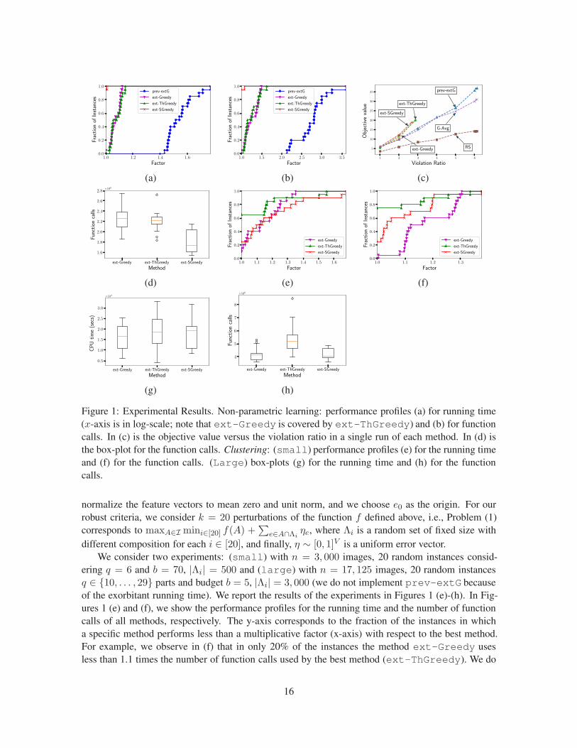
We made 20 random runs considering q = 3 parts and budget b = 5. We report the results inFigures 1 (a)-(d). In Figures 1 (a) and (b), we show the performance profiles for the running time andthe number of function calls of all methods, respectively. The y-axis corresponds to the fraction of theinstances in which a specific method performs less than a multiplicative factor (x-axis) with respectto the best performance. For example, we observe in (b) that in only 20% of the instances the methodprev-extG uses less than 2.5 times the number of function calls used by the best method. We alsonote that any of the three algorithms clearly outperform prev-extG, either in terms of running time(a) or function calls (b). With this, we show empirically that our implementation improvements helpin the performance of the algorithm. We also note that ext-SGreedy is likely to have the bestperformance. Box-plots for the function calls in Figure 1 (d) confirm this fact, since ext-SGreedyhas the lowest median. Each method is presented in the x-axis and the y-axis corresponds to thenumber of function calls (the orange line is the median and circles are outliers). In this figure, wedo not present the results of prev-extG because of the difference in magnitude. Finally, in (c) wepresent the objective values (y-axis) obtained in a single run with respect to the number of feasiblesets needed to cover the given set (x-axis). For example, when the set constructed by each methodis 2 times the size of a feasible set, most of the procedures have an objective value around 10. Weobserve that the stopping rule is useful since the three tested algorithms output a nearly optimalsolution earlier (using around 3 times the size of a feasible set) outperforming prev-extG andthe benchmarks (which need around 6 times), and moreover, at much less computational cost as wementioned before.

2.3.2 Exemplar-based Clustering.

We follow the setup in (Mirzasoleiman et al., 2015). Solving the k-medoid problem is a commonway to select a subset of exemplars that represent a large dataset V (Kaufman and Rousseeuw, 2009).This is done by minimizing the sum of pairwise dissimilarities between elements in A ⊆ V and V .Formally, define L(A) = 1

V

∑

e∈V minv∈A d(e, v), where d : V × V → R+ is a distance functionthat represents the dissimilarity between a pair of elements. By introducing an appropriate auxiliaryelement e0, it is possible to define a new objective f(A) := L({e0}) − L(A + e0) that is monotoneand submodular (Gomes and Krause, 2010), thus maximizing f is equivalent to minimizing L. In ourexperiment, we use the VOC2012 dataset (Everingham et al., 2012). The ground set V correspondsto images, and we want to select a subset of the images that best represents the dataset. Each imagehas several (possible repeated) associated categories such as person, plane, etc. There are around20 categories in total. Therefore, images are represented by feature vectors obtained by counting thenumber of elements that belong to each category, for example, if an image has 2 people and one plane,then its feature vector is (2, 1, 0, . . . , 0) (where zeros correspond to other elements). We choose theEuclidean distance d(e, e′) = ‖xe − xe′‖ where xe, xe′ are the feature vectors for images e, e′. We

15

1.0 1.2 1.4 1.6

Factor

0.0

0.2

0.4

0.6

0.8

1.0

Fractionof

Instances

prev-extG

ext-Greedy

ext-ThGreedy

ext-SGreedy

1.0 1.5 2.0 2.5 3.0 3.5

Factor

0.0

0.2

0.4

0.6

0.8

1.0

Fractionof

Instances

prev-extG

ext-Greedy

ext-ThGreedy

ext-SGreedy

1 2 3 4 5 6

Violation Ratio

5

10

15

20

25

30

35

Objectivevalue

prev-extG

ext-Greedy

ext-ThGreedy

ext-SGreedy

G-Avg

RS

(a) (b) (c)

ext-Greedy ext-ThGreedy ext-SGreedy

Method

1.6

1.8

2.0

2.2

2.4

2.6

2.8

Functioncalls

×106

1.0 1.1 1.2 1.3 1.4 1.5 1.6

Factor

0.0

0.2

0.4

0.6

0.8

1.0

Fractionof

Instances

ext-Greedy

ext-ThGreedy

ext-SGreedy

1.0 1.1 1.2 1.3

Factor

0.0

0.2

0.4

0.6

0.8

1.0

Fractionof

Instances

ext-Greedy

ext-ThGreedy

ext-SGreedy

(d) (e) (f)


Method

0.5

1.0

1.5

2.0

2.5

3.0

CPUtime(secs)

×103


Method

4

5

6

7

8

Functioncalls

×106

(g) (h)

Figure 1: Experimental Results. Non-parametric learning: performance profiles (a) for running time(x-axis is in log-scale; note that ext-Greedy is covered by ext-ThGreedy) and (b) for functioncalls. In (c) is the objective value versus the violation ratio in a single run of each method. In (d) isthe box-plot for the function calls. Clustering: (small) performance profiles (e) for the running timeand (f) for the function calls. (Large) box-plots (g) for the running time and (h) for the functioncalls.

normalize the feature vectors to mean zero and unit norm, and we choose e0 as the origin. For ourrobust criteria, we consider k = 20 perturbations of the function f defined above, i.e., Problem (1)corresponds to maxA∈I mini∈[20] f(A) +

∑

e∈A∩Λiηe, where Λi is a random set of fixed size with

different composition for each i ∈ [20], and finally, η ∼ [0, 1]V is a uniform error vector.We consider two experiments: (small) with n = 3, 000 images, 20 random instances consid-

ering q = 6 and b = 70, |Λi| = 500 and (large) with n = 17, 125 images, 20 random instancesq ∈ {10, . . . , 29} parts and budget b = 5, |Λi| = 3, 000 (we do not implement prev-extG becauseof the exorbitant running time). We report the results of the experiments in Figures 1 (e)-(h). In Fig-ures 1 (e) and (f), we show the performance profiles for the running time and the number of functioncalls of all methods, respectively. The y-axis corresponds to the fraction of the instances in whicha specific method performs less than a multiplicative factor (x-axis) with respect to the best method.For example, we observe in (f) that in only 20% of the instances the method ext-Greedy usesless than 1.1 times the number of function calls used by the best method (ext-ThGreedy). We do

16

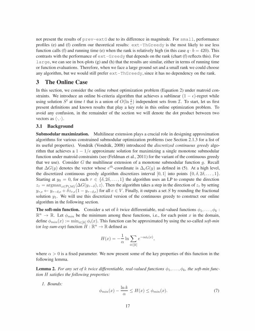
not present the results of prev-extG due to its difference in magnitude. For small, performanceprofiles (e) and (f) confirm our theoretical results: ext-ThGreedy is the most likely to use lessfunction calls (f) and running time (e) when the rank is relatively high (in this case q · b = 420). Thiscontrasts with the performance of ext-Greedy that depends on the rank (chart (f) reflects this). Forlarge, we can see in box-plots (g) and (h) that the results are similar, either in terms of running timeor function evaluations. Therefore, when we face a large ground set and a small rank we could chooseany algorithm, but we would still prefer ext-ThGreedy, since it has no dependency on the rank.

3 The Online Case

In this section, we consider the online robust optimization problem (Equation 2) under matroid con-straints. We introduce an online bi-criteria algorithm that achieves a sublinear (1 − ǫ)-regret whileusing solution St at time t that is a union of O(ln 1

ǫ ) independent sets from I . To start, let us firstpresent definitions and known results that play a key role in this online optimization problem. Toavoid any confusion, in the remainder of the section we will denote the dot product between twovectors as 〈·, ·〉.3.1 Background

Submodular maximization. Multilinear extension plays a crucial role in designing approximationalgorithms for various constrained submodular optimization problems (see Section 2.1.3 for a list ofits useful properties). Vondrák (Vondrák, 2008) introduced the discretized continuous greedy algo-rithm that achieves a 1 − 1/e approximate solution for maximizing a single monotone submodularfunction under matroid constraints (see (Feldman et al., 2011) for the variant of the continuous greedythat we use). Consider G the multilinear extension of a monotone submodular function g. Recallthat ∆G(y) denotes the vector whose eth-coordinate is ∆eG(y) as defined in (5). At a high level,the discretized continuous greedy algorithm discretizes interval [0, 1] into points {0, δ, 2δ, . . . , 1}.Starting at y0 = 0, for each τ ∈ {δ, 2δ, . . . , 1} the algorithm uses an LP to compute the directionzτ = argmaxz∈P(M)〈∆G(yτ−δ), z〉. Then the algorithm takes a step in the direction of zτ by settingyτ,e ← yτ−δ,e + δzτ,e(1− yτ−δ,e) for all e ∈ V . Finally, it outputs a set S by rounding the fractionalsolution y1. We will use this discretized version of the continuous greedy to construct our onlinealgorithm in the following section.

The soft-min function. Consider a set of k twice differentiable, real-valued functions φ1, . . . , φk :Rn → R. Let φmin be the minimum among these functions, i.e., for each point x in the domain,

define φmin(x) := mini∈[k] φi(x). This function can be approximated by using the so-called soft-min

(or log-sum-exp) function H : Rn → R defined as

H(x) = − 1

αln∑

i∈[k]

e−αφi(x),

where α > 0 is a fixed parameter. We now present some of the key properties of this function in thefollowing lemma.

Lemma 2. For any set of k twice differentiable, real-valued functions φ1, . . . , φk , the soft-min func-

tion H satisfies the following properties:

1. Bounds:

φmin(x)−ln k

α≤ H(x) ≤ φmin(x). (7)

17

2. Gradient:

∇H(x) =∑

i∈[k]

pi(x)∇φi(x), (8)

where pi(x) := e−αφi(x)/∑

j∈[k] e−αφj(x). Clearly, if ∇φi ≥ 0 for all i ∈ [k], then ∇H ≥ 0.

3. Hessian:

∂2H(x)

∂xe1∂xe2=∑

i∈[k]

pi(x)

(

−α∂φi(x)

∂xe1

∂φi(x)

∂xe2+

∂2φi(x)

∂xe1∂xe2

)

+ α∇e1H(x)∇e2H(x) (9)

Moreover, if for all i ∈ [k] we have

∣

∣

∣

∂φi

∂xe1

∣

∣

∣ ≤ L1, and

∣

∣

∣

∂2φi

∂xe1∂xe2

∣

∣

∣ ≤ L2, then

∣

∣

∣

∂2H∂xe1

∂xe2

∣

∣

∣ ≤2αL2

1 + L2.

4. Comparing the average of the φi functions with H: given α > 0 we have

H(x) ≤∑

i∈[k]

pi(x)φi(x) ≤ H(x) +lnα

α+

ln k

α+

k

α. (10)

Therefore, for α > 0 sufficiently large∑

i∈[k] pi(x)φi(x) is a good approximation of H(x).

For other properties and applications, we refer the interested reader to (Calafiore and El Ghaoui,2014). Now, we present a lemma which is used to prove the main result in the online case, Theorem2.

Lemma 3. Fix a parameter δ > 0. Consider T collections of k twice-differentiable functions, namely

{φ1i }i∈[k], . . . , {φT

i }i∈[k]. Assume 0 ≤ φti(x) ≤ 1 for any x in the domain, for all t ∈ [T ] and i ∈ [k].

Define the corresponding sequence of soft-min functions H1, . . . ,HT , with common parameter α > 0.

Then, any two sequences of points {xt}t∈[T ], {yt}t∈[T ] ⊆ [0, 1]V with |xt − yt| ≤ δ satisfy

∑

t∈[T ]

Ht(yt)−∑

t∈[T ]

Ht(xt) ≥∑

t∈[T ]

〈∇Ht(xt), yt − xt〉 −O(

Tn2δ2α)

.

For a proof of these lemmas, we refer to the Appendix.

3.2 Online Algorithm and Analysis

Turning our attention to the online robust optimization problem (2), we are immediately faced withtwo challenges. First, we need to find a direction zt that is good for all k submodular functions inan online fashion. In the offline case, we used the function g(S) = 1

k ·∑k

i=1min{fi(S), γ} andits multilinear extension to find such a direction (see Section 2.1.3). To resolve this issue, we usea soft-min function that converts robust optimization over k functions into optimizing of a singlefunction. Secondly, robust optimization leads to non-convex and non-smooth optimization combinedwith online arrival of such submodular functions. To deal with this, we use the Follow-the-Perturbed-Leader (FPL) online algorithm introduced by Kalai and Vempala (2005).

For any collection of monotone submodular functions {f ti }i∈[k] played by the adversary, we define

the soft-min function with respect to the corresponding multilinear extensions {F ti }i∈[k] as Ht(y) :=

− 1α ln

∑

i∈[k] e−αF t

i (y), where α > 0 is a suitable parameter. Recall we assume functions f ti taking

values in [0, 1], then their multilinear extensions F ti also take values in [0, 1]. The following properties

18

of the soft-min function as defined in the previous section are easy to verify and crucial for our result.

1. Approximation: mini∈[k] Fti (y)−

ln k

α≤ Ht(y) ≤ mini∈[k] F

ti (y).

2. Gradient: ∇Ht(y) =∑

i∈[k] pti(y)∇F t

i (y), where pti(y) ∝ e−αF ti (y) for all i ∈ [k].

Note that as α increases, the soft-min function Ht becomes a better approximation of mini∈[k]{F ti },

however, its smoothness degrades (see Property (9) in Section 3.1). On the other hand, the secondproperty shows that the gradient of the soft-min function is a convex combination of the gradients ofthe multilinear extensions, which allows us to optimize all the functions at the same time. Indeed,define ∆eH

t(y) :=∑

i∈[k] pti(y)∆eF

ti (y) = (1 − ye)∇eH

t(y). At each stage t ∈ [T ], we use the

information from the gradients previously observed, in particular, {∆H1, · · · ,∆Ht−1} to decide theset St. To deal with adversarial input functions, we use the FPL algorithm (Kalai and Vempala, 2005)and the following guarantee about the algorithm.

Theorem 4 (Kalai and Vempala (2005)). Let s1, . . . , sT ∈ S be a sequence of rewards. The FPL

algorithm 6 (in the Appendix) with parameter η ≤ 1 outputs decisions d1, . . . , dT with regret

maxd∈D

∑

t∈[T ]

〈st, d〉 − E

∑

t∈[T ]

〈st, dt〉

≤ O

(

poly(n)

(

ηT +1

Tη

))

.

For completeness, we include the original setup and the algorithm in the Appendix.Our online algorithm works as follows: first, given 0 < ǫ < 1 we denote ℓ := ⌈ln 1

ǫ ⌉. We considerthe following discretization indexed by τ ∈ {0, δ, 2δ, . . . , ℓ} and construct fractional solutions ytτ foreach iteration t and discretization index τ . At each iteration t, ideally we would like to construct{ytτ}ℓτ=0 by running the continuous greedy algorithm using the soft-min function Ht and then playSt using these fractional solutions. But in the online model, function Ht is revealed only after playingset St. To remedy this, we aim to construct ytτ using FPL algorithm based on gradients {∇Hj}t−1

j=1

obtained from previous iterations. Thus we have multiple FPL instances, one for each discretizationparameter, being run by the algorithm. Finally, at the end of iteration t, we have a fractional vectorytℓ which belongs to ℓ · P(M) ∩ [0, 1]V and therefore can be written, fractionally, as a union of ℓindependent sets using the matroid union theorem (Schrijver, 2003).

We round the fractional solution ytℓ using the randomized swap rounding (or randomized pipagerounding) proposed by Chekuri et al. (2010) for matroidMℓ to obtain the set St to be played at timet. The following theorem from (Chekuri et al., 2010) gives the necessary property of the randomizedswap rounding that we use.

Theorem 5 (Theorem II.1, (Chekuri et al., 2010)). Let f be a monotone submodular function and

F be its multilinear extension. Let x ∈ P(M′) be a point in the polytope of matroid M′ and S′ a

random independent set obtained from it by randomized swap rounding. Then, E[f(S′)] ≥ F (x).

Below, we formalize the details in Algorithm 4 (observe that ℓ/δ ∈ Z+). In order to get sub-linear regret for the FPL algorithm 6, Kalai and Vempala (2005) assume a couple of conditions on theproblem (see Appendix). Similarly, for our online model we need to consider the following for anyt ∈ [T ]:

19

Algorithm 4 OnlineSoftMin algorithm

Input: learning parameter η > 0, ǫ > 0, α = nT , discretization δ = n−1T−1, and ℓ = ⌈ln 1ǫ ⌉.

Output: sequence of sets S1, . . . , ST .1: Sample q ∼ [0, 1/η]V

2: for t = 1 to T do

3: yt0 = 04: for τ ∈ {δ, 2δ, . . . , ℓ} do

5: Compute ztτ = argmaxz∈P(M)

⟨

∑t−1j=1∆Hj(yjτ−δ) + q, z

⟩

.

6: Update For each e ∈ V , ytτ,e = ytτ−δ,e + δ(1 − ytτ−δ,e)ztτ,e.

7: Play St ← Rounding(

ytℓ)

. Receive and observe new collection {f ti }i∈[k].

1. bounded diameter of P(M), i.e., for all z, z′ ∈ P(M), ‖z − z′‖1 ≤ D;

2. for all y, z ∈ P(M), we require∣

∣〈z,∆Ht(y)〉∣

∣ ≤ L;

3. for all y ∈ P(M), we require ‖∆Ht(y)‖1 ≤ A,

Now, we give a complete proof of Theorem 2 for any given learning parameter η > 0, but thefinal result follows with η =

√

D/LAT and assuming L ≤ n, A ≤ n and D ≤ √n, which gives aO(n5/4) dependency on the dimension in the regret.

Proof of Theorem 2. Consider the sequence of multilinear extensions {F 1i }i∈[k], . . . , {F T

i }i∈[k] de-rived from the monotone submodular functions f t

i obtained during the dynamic process. Since f ti ’s

have value in [0, 1], we have 0 ≤ F ti (y) ≤ 1 for any y ∈ [0, 1]V and i ∈ [k]. Consider the correspond-

ing soft-min functions Ht for collection {F ti }i∈[k] with α = nT for all t ∈ [T ]. Denote ℓ = ⌈ln 1

ǫ ⌉and fix τ ∈ {δ, 2δ, . . . , ℓ} with δ = n−1T−1. According to the update in Algorithm 4, {ytτ}t∈[T ] and{ytτ−δ}t∈[T ] satisfy conditions of Lemma 3. Thus, we obtain

∑

t∈[T ]

Ht(ytτ )−Ht(ytτ−δ) ≥∑

t∈[T ]

⟨

∇Ht(ytτ−δ), ytτ − ytτ−δ

⟩

−O(

Tn2δ2α)

.

Then, since the update is ytτ,e = ytτ−δ,e + δ(1 − ytτ−δ,e)ztτ,e, we get

∑

t∈[T ]

Ht(ytτ )−Ht(ytτ−δ) ≥ δ∑

t∈[T ]

∑

e∈V

∇eHt(ytτ−δ)(1− ytτ−δ,e)z

tτ,e −O

(

Tn2δ2α)

= δ∑

t∈[T ]

⟨

∆Ht(ytτ−δ), ztτ

⟩

−O(

Tn2δ2α)

. (11)

Observe that an FPL algorithm is implemented for each τ , so we can state a regret bound for eachτ by using Theorem 4. Specifically,

E

∑

t∈[T ]

⟨

∆Ht(ytτ−δ), ztτ

⟩

≥ maxz∈P(M)

E

∑

t∈[T ]

⟨

∆Ht(ytτ−δ), z⟩

− Rη,

20

where Rη = ηLAT + Dη is the regret guarantee for a given η > 0. By taking expectation in (11) and

using the regret bound we just mentioned, we obtain

E

[

∑

t∈[T ]

Ht(ytτ )−Ht(ytτ−δ)

]

≥ δ

maxz∈P(M)

E

∑

t∈[T ]

⟨

∆Ht(ytτ−δ), z⟩

− δRη −O(Tn2δ2α)

≥ δE

∑

t∈[T ]

Ht(x∗)−∑

i∈[k]

pti(ytτ−δ)F

ti (y

tτ−δ)

− δRη −O(Tn2δ2α), (12)

where x∗ = 1S∗ is the indicator vector of the true optimum S∗ for maxS∈I∑

t∈[T ]mini∈[k] fti (S).

Observe that (12) follows from monotonicity and submodularity of each f ti , specifically we know that

⟨

∆Ht(y), z⟩

=∑

i∈[k]

pti(y)⟨

∆F ti (y), z

⟩

≥∑

i∈[k]

pti(y)Fti (x

∗)−∑

i∈[k]

pti(y)Fti (y) (eq. (6))

≥ F tmin(x

∗)−∑

i∈[k]

pti(y)Fti (y)

≥ Ht(x∗)−∑

i∈[k]

pti(y)Fti (y).

By applying property (10) of the soft-min in expression (12) we get

E

∑

t∈[T ]

Ht(ytτ )−Ht(ytτ−δ)

≥δE

∑

t∈[T ]

Ht(x∗)−Ht(ytτ−δ)

− δRη −O(Tn2δ2α)

− δT

(

lnα

α+

ln k

α+

k

α

)

, (13)

Given the choice of α and δ, the last two terms in the right-hand side of inequality (13) are smallcompared to Rη, so by re-arranging terms we can state the following

∑

t∈[T ]

Ht(x∗)− E

∑

t∈[T ]

Ht(ytτ )

≤ (1− δ)

∑

t∈[T ]

Ht(x∗)− E

∑

t∈[T ]

Ht(ytτ−δ)

+ 2δRη

By iterating ℓδ times in τ , we get

∑

t∈[T ]

Ht(x∗)− E

∑

t∈[T ]

Ht(ytℓ)

≤ (1− δ)ℓδ

∑

t∈[T ]

Ht(x∗)−∑

t∈[T ]

Ht(yt0)

+O(

(1− (1− δ)ℓδ )Rη

)

≤ ǫ

∑

t∈[T ]

Ht(x∗) + ln k

+O ((1− ǫ)Rη) ,

where in the last inequality we used (1− δ) ≤ e−δ and ℓ = ⌈ln 1ǫ ⌉. Given that the term ǫ ln k is small

(for ǫ sufficiently small) we can bound it by O(Rη). Since α is sufficiently large, we can apply the

21

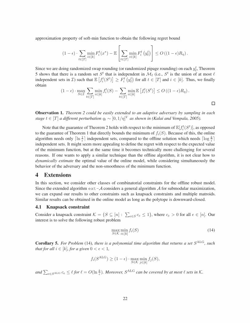
approximation property of soft-min function to obtain the following regret bound

(1− ǫ) ·∑

t∈[T ]

mini∈[k]

F ti (x

∗)− E

∑

t∈[T ]

mini∈[k]

F ti

(

ytℓ)

≤ O ((1− ǫ)Rη) .

Since we are doing randomized swap rounding (or randomized pipage rounding) on each ytℓ, Theorem5 shows that there is a random set St that is independent in Mℓ (i.e., St is the union of at most ℓindependent sets in I) such that E

[

f ti (S

t)]

≥ F ti

(

ytℓ)

for all t ∈ [T ] and i ∈ [k]. Thus, we finallyobtain

(1− ǫ) ·maxS∈I

∑

t∈[T ]

mini∈[k]

f ti (S)−

∑

t∈[T ]

mini∈[k]

E[

f ti (S

t)]

≤ O ((1− ǫ)Rη) .

Observation 1. Theorem 2 could be easily extended to an adaptive adversary by sampling in each

stage t ∈ [T ] a different perturbation qt ∼ [0, 1/η]V as shown in (Kalai and Vempala, 2005).

Note that the guarantee of Theorem 2 holds with respect to the minimum of E[f ti (S

t)], as opposedto the guarantee of Theorem 1 that directly bounds the minimum of fi(S). Because of this, the onlinealgorithm needs only ⌈ln 1

ǫ ⌉ independent sets, compared to the offline solution which needs ⌈log kǫ ⌉

independent sets. It might seem more appealing to define the regret with respect to the expected valueof the minimum function, but at the same time it becomes technically more challenging for severalreasons. If one wants to apply a similar technique than the offline algorithm, it is not clear how todynamically estimate the optimal value of the online model, while considering simultaneously thebehavior of the adversary and the non-smoothness of the minimum function.

4 Extensions

In this section, we consider other classes of combinatorial constraints for the offline robust model.Since the extended algorithm ext-A considers a general algorithm A for submodular maximization,we can expand our results to other constraints such as knapsack constraints and multiple matroids.Similar results can be obtained in the online model as long as the polytope is downward-closed.

4.1 Knapsack constraint

Consider a knapsack constraint K = {S ⊆ [n] :∑

e∈S ce ≤ 1}, where ce > 0 for all e ∈ [n]. Ourinterest is to solve the following robust problem

maxS∈K

mini∈[k]

fi(S) (14)

Corollary 5. For Problem (14), there is a polynomial time algorithm that returns a set SALG, such

that for all i ∈ [k], for a given 0 < ǫ < 1,


S∈Kminj∈[k]

fj(S),

and∑

e∈SALG ce ≤ ℓ for ℓ = O(ln kǫ ). Moreover, SALG can be covered by at most ℓ sets in K.

22

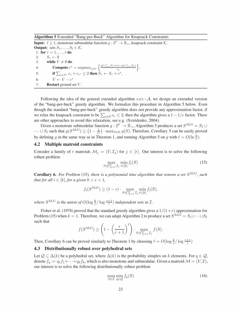
Algorithm 5 Extended “Bang-per-Buck” Algorithm for Knapsack Constraints

Input: ℓ ≥ 1, monotone submodular function g : 2V → R+, knapsack constraint K.Output: sets S1, . . . , Sℓ ∈ K.

1: for τ = 1, . . . , ℓ do

2: Sτ ← ∅3: while V 6= ∅ do

4: Compute e∗ = argmaxe∈V

{

g(∪τj=1

Sj+e)−g(∪τj=1

Sj)

ce

}

.

5: if∑

e∈Sτ ce + ce∗ ≤ 2 then Sτ ← Sτ + e∗.

6: V ← V − e∗

7: Restart ground set V .

Following the idea of the general extended algorithm ext-A, we design an extended versionof the “bang-per-buck” greedy algorithm. We formalize this procedure in Algorithm 5 below. Eventhough the standard “bang-per-buck” greedy algorithm does not provide any approximation factor, ifwe relax the knapsack constraint to be

∑

e∈S ce ≤ 2, then the algorithm gives a 1− 1/e factor. Thereare other approaches to avoid this relaxation, see e.g. (Sviridenko, 2004).

Given a monotone submodular function g : 2V → R+, Algorithm 5 produces a set SALG = S1 ∪· · · ∪ Sℓ such that g(SALG) ≥

(

1− 1eℓ

)

·maxS∈K g(S). Therefore, Corollary 5 can be easily proved

by defining g in the same way as in Theorem 1, and running Algorithm 5 on g with ℓ = O(ln kǫ ).

4.2 Multiple matroid constraints

Consider a family of r matroids Mj = (V,Ij) for j ∈ [r]. Our interest is to solve the followingrobust problem

maxS∈

⋂rj=1

Ijmini∈[k]

fi(S) (15)



fi(SALG) ≥ (1− ǫ) · max

S∈⋂r

j=1Ijmini∈[k]

fi(S),

where SALG is the union of O(log kǫ / log

r+1r ) independent sets in I .

Fisher et al. (1978) proved that the standard greedy algorithm gives a 1/(1+r) approximation forProblem (15) when k = 1. Therefore, we can adapt Algorithm 2 to produce a set SALG = S1∪· · ·∪Sℓ

such that

f(SALG) ≥(

1−(

r

r + 1

)ℓ)

· maxS∈

⋂rj=1

Ijf(S).

Then, Corollary 6 can be proved similarly to Theorem 1 by choosing ℓ = O(log kǫ / log

r+1r )

4.3 Distributionally robust over polyhedral sets

Let Q ⊆ ∆(k) be a polyhedral set, where ∆(k) is the probability simplex on k elements. For q ∈ Q,denote fq := q1f1+· · ·+qkfk, which is also monotone and submodular. Given a matroidM = (V,I),our interest is to solve the following distributionally robust problem

maxS∈I

minq∈Q

fq(S) (16)

23

Denote by Vert(Q) the set of extreme points of Q, which is finite since Q is polyhedral. Then,Problem (16) is equivalent to maxS∈I minq∈Vert(Q) fq(S). Then, we can easily derive Corollary 7(below) by applying Theorem 1 in the equivalent problem. Note that when Q is the simplex we getthe original Theorem 1.




S∈Iminq∈Q

fq(S),

with SALG = S1 ∪ · · · ∪ Sℓ for ℓ = O(log |Vert(Q)|ǫ ) and S1, . . . , Sℓ ∈ I .

Acknowledgements

This research was partially supported by NSF Award CCF-1717947, NSF CAREER Award CMMI-1452463, an IBM Ph.D. fellowship, and a Microsoft Research Ph.D. fellowship. We also thank Shab-bir Ahmed for the discussions about the distributionally robust problem (16).

References

A.A. Ageev and M.I. Sviridenko. Pipage rounding: A new method of constructing algorithms withproven performance guarantee. Journal of Combinatorial Optimization, 8(3):307–328, 2004.

Nima Anari, Nika Haghtalab, Seffi Naor, Sebastian Pokutta, Mohit Singh, and Alfredo Torrico. Struc-tured robust submodular maximization: offline and online algorithms. In Proceedings of the 22nd

International Conference on Artificial Intelligence and Statistics (AISTATS), pages 3128–3137,2019.

Ashwinkumar Badanidiyuru and Jan Vondrák. Fast algorithms for maximizing submodular functions.In Proceedings of the 25th Annual ACM-SIAM Symposium on Discrete Algorithms (SODA), pages1497–1514, 2014.

Ilija Bogunovic, Slobodan Mitrovic, Jonathan Scarlett, and Volkan Cevher. Robust submodular max-imization: A non-uniform partitioning approach. In Proceedings of the 34th International Confer-

ence on Machine Learning (ICML), pages 508–516, 2017.

Niv Buchbinder and Moran Feldman. Deterministic algorithms for submodular maximization prob-lems. In Proceedings of the 27th Annual ACM-SIAM Symposium on Discrete Algorithms (SODA),pages 392–403, 2016.

Niv Buchbinder, Moran Feldman, Joseph Seffi Naor, and Roy Schwartz. Submodular maximizationwith cardinality constraints. In Proceedings of the 25th Annual ACM-SIAM Symposium on Discrete

Algorithms (SODA), pages 1433–1452, 2014.

Niv Buchbinder, Moran Feldman, and Roy Schwartz. Comparing apples and oranges: Query trade-offin submodular maximization. Mathematics of Operations Research, 42(2):308–329, 2016.

Giuseppe C. Calafiore and Laurent El Ghaoui. Optimization Models. Cambridge University, 2014.

Gruia Calinescu, Chandra Chekuri, Martin Pál, and Jan Vondrák. Maximizing a monotone submodu-lar function subject to a matroid constraint. SIAM Journal on Computing, 40(6):1740–1766, 2011.

24

Chandra Chekuri, Jan Vondrak, and Rico Zenklusen. Dependent randomized rounding via exchangeproperties of combinatorial structures. In Proceedings of the 51st Annual Symposium on Founda-

tions of Computer Science (FOCS), pages 575–584, 2010.

Robert S. Chen, Brendan Lucier, Yaron Singer, and Vasilis Syrgkanis. Robust optimization for non-convex objectives. In Proceedings of the 31st International Conference on Neural Information

Processing Systems (NeurIPS), pages 4708–4717, 2017.

Wei Chen, Tian Lin, Zihan Tan, Mingfei Zhao, and Xuren Zhou. Robust influence maximization. InProceedings of the 22nd ACM SIGKDD Conference on Knowledge Discovery and Data Mining

(KDD), pages 795–804, 2016.

Abhimanyu Das and David Kempe. Algorithms for subset selection in linear regression. In Pro-

ceedings of the 40th Annual ACM Symposium on the Theory of Computing (STOC), pages 45–54,2008.

Alina Ene and Huy L. Nguyen. Constrained submodular maximization: Beyond 1/e. In Proceedings

of the 57th Annual Symposium on Foundations of Computer Science (FOCS), pages 248–257, 2016.

M. Everingham, L. Van Gool, C. K. I. Williams, J. Winn, and A. Zisserman. ThePASCAL Visual Object Classes Challenge 2012 (VOC2012) Results. http://www.pascal-network.org/challenges/VOC/voc2012/workshop/index.html, 2012.

Moran Feldman, Joseph Naor, and Roy Schwartz. A unified continuous greedy algorithm for submod-ular maximization. In Proceedings of the 52nd Annual Symposium on Foundations of Computer

Science (FOCS), pages 570–579, 2011.

Marshall L. Fisher, George L. Nemhauser, and Laurence A. Wolsey. An analysis of approximationsfor maximizing submodular set functions—ii. In Polyhedral combinatorics, pages 73–87. Springer,1978.

Daniel Golovin, Andreas Krause, and Matthew Streeter. Online submodular maximization under amatroid constraint with application to learning assignments. Technical Report, arXiv, 2014.

Ryan Gomes and Andreas Krause. Budgeted nonparametric learning from data streams. In Proceed-

ings of the 27th International Conference on Machine Learning (ICML), pages 391–398, 2010.

Xinran He and David Kempe. Robust influence maximization. In Proceedings of the 22nd ACM

SIGKDD Conference on Knowledge Discovery and Data Mining (KDD), pages 885–894, 2016.

Adam Kalai and Santosh Vempala. Efficient algorithms for online decision problems. Journal of

Computer and System Sciences, 71(3):291–307, 2005.

L. Kaufman and P. J. Rousseeuw. Finding groups in data: an introduction to cluster analysis, volume344. Wiley-Interscience, 2009.

Ehsan Kazemi, Morteza Zadimoghaddam, and Amin Karbasi. Scalable deletion-robust submodularmaximization: Data summarization with privacy and fairness constraints. In Proceedings of the

35th International Conference on Machine Learning (ICML), volume 80, pages 2544–2553, 2018.

25

David Kempe, Jon Kleinberg, and Éva Tardos. Maximizing the spread of influence through a socialnetwork. Theory of Computing, 11(4):105–147, 2003.

Andreas Krause and Carlos Guestrin. Near-optimal nonmyopic value of information in graphicalmodels. In Proceedings of the 21st Conference on Uncertainty in Artificial Intelligence (UAI),pages 324–331, 2005a.

Andreas Krause and Carlos Guestrin. Near-optimal nonmyopic value of information in graphicalmodels. In Proceedings of the 21st Conference on Uncertainty in Artificial Intelligence (UAI),pages 324–331, 2005b.

Andreas Krause, H. Brendan McMahan, Carlos Guestrin, and Anupam Gupta. Robust submodularobservation selection. Journal of Machine Learning Research, 9:2761–2801, 2008a.

Andreas Krause, Ajit Singh, and Carlos Guestrin. Near-optimal sensor placements in gaussian pro-cesses: Theory, efficient algorithms and empirical studies. Journal of Machine Learning Research,9:235–284, 2008b.

Andreas Krause, Ram Rajagopal, Anupam Gupta, and Carlos Guestrin. Simultaneous placement andscheduling of sensors. In Proceedings of the 8th ACM/IEEE Conference on Information Processing

in Sensor Networks (IPSN), pages 181–192, 2009.

Jon Lee, Vahab S Mirrokni, Viswanath Nagarajan, and Maxim Sviridenko. Non-monotone submodu-lar maximization under matroid and knapsack constraints. In Proceedings of the 41st Annual ACM

Symposium on the Theory of Computing (STOC), pages 323–332, 2009.

Hui Lin and Jeff A. Bilmes. How to select a good training-data subset for transcription: submodularactive selection for sequences. In Proceedings of the 10th Annual Conference of the International

Speech Communication Association (INTERSPEECH), pages 2859–2862, 2009.

M. Minoux. Accelerated greedy algorithms for maximizing submodular set functions. Optimization

Techniques, LNCS, pages 234–243, 1978.

Baharan Mirzasoleiman, Ashwinkumar Badanidiyuru, Amin Karbasi, Jan Vondrák, and AndreasKrause. Lazier than lazy greedy. In Proceedings of the 29th AAAI Conference on Artificial In-

telligence (AAAI), pages 1812–1818, 2015.

Marko Mitrovic, Ehsan Kazemi, Morteza Zadimoghaddam, and Amin Karbasi. Data summarizationat scale: A two-stage submodular approach. In Proceedings of the 35th International Conference

on Machine Learning (ICML), pages 3593–3602, 2018.

George L. Nemhauser, Laurence A. Wolsey, and Marshall L. Fisher. An analysis of approximationsfor maximizing submodular set functions—i. Mathematical Programming, 14(1):265–294, 1978.

James B. Orlin, Andreas S. Schulz, and Rajan Udwani. Robust monotone submodular function maxi-mization. In Proceedings of the 18th International Conference on Integer Programming and Com-

binatorial Optimization (IPCO), pages 312–324, 2016.

Thomas Powers, Jeff Bilmes, David W. Krout, and Les Atlas. Constrained robust submodular sensorselection with applications to multistatic sonar arrays. In Proceedings of the 19th International

Conference on Information Fusion (FUSION), pages 2179–2185, 2016a.

26

Thomas Powers, Jeff Bilmes, Scott Wisdom, David W Krout, and Les Atlas. Constrained robustsubmodular optimization. In NIPS OPT2016 workshop, 2016b.

Alexander Rakhlin. Lecture notes on online learning. Draft, April, 2009.

Alexander Schrijver. Combinatorial optimization: polyhedra and efficiency, volume 24. SpringerScience & Business Media, 2003.

Tasuku Soma. No-regret algorithms for online k-submodular maximization. In Proceedings of Ma-

chine Learning Research, volume 89 of Proceedings of Machine Learning Research, pages 1205–1214, 2019.

Matthew Staib, Bryan Wilder, and Stefanie Jegelka. Distributionally robust submodular maximization.CoRR, abs/1802.05249, 2018.

Matthew Streeter and Daniel Golovin. An online algorithm for maximizing submodular functions.In Proceedings of the 21st International Conference on Neural Information Processing Systems

(NeurIPS), pages 1577–1584, 2008.

Maxim Sviridenko. A note on maximizing a submodular set function subject to a knapsack constraint.Operations Research Letters, 32(1):41–43, 2004.

A. Tsanas, M. A. Little, P. E. McSharry, and L. O. Ramig. Enhanced classical dysphonia measuresand sparse regression for telemonitoring of parkinson’s disease progression. In Proceedings of the

35th IEEE International Conference on Acoustics, Speech and Signal Processing (ICASSP), pages594–597, 2010.

Jan Vondrák. Optimal approximation for the submodular welfare problem in the value oracle model.In Proceedings of the 40th Annual ACM Symposium on the Theory of Computing (STOC), pages67–74, 2008.

Bryan Wilder. Equilibrium computation and robust optimization in zero sum games with submodularstructure. arXiv, 2017.

Laurence A. Wolsey. An analysis of the greedy algorithm for the submodular set covering problem.Combinatorica, 2(4):385–393, 1982.

Mingrui Zhang, Lin Chen, Hamed Hassani, and Amin Karbasi. Online continuous submodular max-imization: From full-information to bandit feedback. In Proceedings of the 32nd International

Conference on Neural Information Processing Systems (NeurIPS), pages 9210–9221, 2019.

A Remaining Proofs

Proof of Corollary 3. Denote by r the rank of matroidM. Let S∗ = {e∗1, . . . , e∗r} and S = {e1, . . . , er}be the optimal set and the set obtained with the algorithm, respectively. W.l.o.g, we can assume thatS∗ and SG are both basis inM, so there exists a bijection φ such that φ(ei) = e∗i for all i ∈ [r]. De-note by Si−1 = {e1, . . . , ei−1} the set of elements after iteration i − 1. Observe that if ei is the nextelement chosen by the algorithm and the current threshold value is w, then we get the inequalities

gSi−1(x) =

{

≥ w if x = ei≤ w/(1 − δ) if x ∈ V s.t. Si−1 + x ∈ I

27

This imples that gSi−1(ei) ≥ (1−δ)fSi−1

(x) for all x ∈ V \Si−1 such that Si−1+x ∈ I . In particularfor x = e∗i we have then

(1− δ)gSi−1(e∗i ) ≤ g(Si)− g(Si−1).

On the other hand, if we apply submodularity twice we get

g(S∗)− g(S) ≤K∑

i=1

gS(e∗i ) ≤

K∑

i=1

gSi−1(e∗i )

Using the previous two inequalities we get

(1− δ)[g(S∗)− g(S)] ≤K∑

i=1

g(Si)− g(Si−1) = g(S).

So we finally obtain

g(S) ≥(

1− 1

2− δ

)

· g(S∗).

Proof of Lemma 2. We will just prove properties 1 and 4, since the rest is a straightforward calcula-tion.

1. First, for all i ∈ [k] we have e−αφi(x) ≤ e−αφmin(x). Thus,

H(x) = − 1

αln∑

i∈[k]

e−αφi(x) ≥ − 1

αln(

ke−αφmin(x))

= φmin(x)−ln k

α

On the other hand,∑

i∈[k] e−αφi(x) ≥ e−αφmin(x). Hence,

H(x) ≤ − 1

αln(

e−αφmin(x))

= φmin(x).

4. Let us consider sets A1 = {i ∈ [k] : φi(x) ≤ φmin(x) + (lnα)/α} and A2 = {i ∈ [k] :φi(x) > φmin(x) + (lnα)/α}. Our intuitive argument is the following: when α is sufficientlylarge, those pi(x)’s with i ∈ A2 are exponentially small, and pi(x)’s with i ∈ A1 go to auniform distribution over elements in A1. First, observe that for each i ∈ A2 we have

pi(x) =e−αφi(x)

∑

i∈[k] e−αφi(x)

<e−α[φmin(x)+(lnα)/α]

e−αφmin(x)=

1

α,

so∑

i∈A2pi(x)φi(x) ≤ k

α . On the other hand, for any i ∈ A1 we have

∑

i∈A1

pi(x)φi(x) ≤(

φmin(x) +lnα

α

)

∑

i∈A1

pi(x) ≤ H(x) +lnα

α+

ln k

α

where in the last inequality we used the approximation property of the soft-min function. There-fore,

∑

i∈[k]

pi(x)φi(x) ≤ H(x) +lnα

α+

ln k

α+

k

α.

Finally, the other inequality is clear since∑

i∈[k] pi(x)φi(x) ≥ φmin(x) ≥ H(x).

28

Proof of Lemma 3. For every t ∈ [T ] define a matroidMt = (V × {t},I × {t}) = (Vt,It). Giventhis, the union matroid is given by a ground set V [T ] =

⋃Tt=1 Vt, and independent set family I [T ] =

{S ⊆ V 1:T : S ∩ Vt ∈ It}. Define H(X) :=∑

t∈[T ]Ht(xt) for any matrix X ∈ P(M)T , where xt

denotes the t-th column of X. Clearly,∇(e,t)H(X) = ∇eHt(xt). Moreover, the Hessian corresponds

to

∇2(e1,t),(e2,s)

H(X) =

{

0 if t 6= s∇2

e1,e2Ht(xt) if t = s

Consider any X,Y ∈ P(M)T with |yte − xte| ≤ δ. Therefore, a Taylor’s expansion of H gives

H(Y ) = H(X) +∇H(X)(Y −X) +1

2(Y −X)⊤∇2

H(ξ)(Y −X)

where ξ is on the line between X and Y . If we expand the previous expression we obtain

H(Y )−H(X) =∑

t∈[T ]

⟨

∇Ht(xt), yt − xt⟩

+1

2

∑

e1,e2∈V

∑

t∈[T ]

(yte1 − xte1)∇2e1,e2H

t(ξ)(yte2 − xte2)

Finally, by using property 3 in Lemma 2 and by bounding the Hessian (and ussing the fact thatφti(x) ∈ [0, 1]) we get

H(Y )−H(X) ≥∑

t∈[T ]

⟨


−O(Tn2δ2α),

which is equivalent to

∑

t∈[T ]

Ht(yt)−∑

t∈[T ]

Ht(xt) ≥∑

t∈[T ]

⟨


−O(Tn2δ2α).

B Follow-the-Perturbed-Leader Algorithm

In this section, we briefly recall the well-known Follow-the-Perturbed-Leader (FPL) algorithm intro-duced in (Kalai and Vempala, 2005) and used in many online optimization problems (see e.g., (Rakhlin,2009)). The classical online learning framework is as follows: Consider a dynamic process over Ttime steps. In each stage t ∈ [T ], a decision-maker has to choose a point dt ∈ D from a fixed (possiblyinfinite) set of actions D ⊆ R

n, then an adversary chooses a vector st from a set S . Finally, the playerobserves vector st and receives reward 〈st, dt〉, and the process continues. The goal of the player is tomaximize the total reward

∑

t∈[T ]〈st, dt〉, and we compare her performance with respect to the bestsingle action picked in hindsight, i.e., maxd∈D

∑

t∈[T ]〈st · d〉. This performance with respect to thebest single action in hindsight is called (expected) regret, formally:

Regret(T ) = maxd∈D

∑

t∈[T ]

〈st, d〉 − E

∑

t∈[T ]

〈st, dt〉

.

29

Kalai and Vempala (2005) showed that even if one has only access to a linear programming oraclefor D, i.e., we can efficiently solve maxd∈D〈s, d〉 for any s ∈ S , then the FPL algorithm 6 achievessub-linear regret, specifically O(

√T ).

In order to state the main result in (Kalai and Vempala, 2005), we need the following. We assumethat the decision set D has diameter at most D, i.e., for all d, d′ ∈ D, ‖d− d′‖1 ≤ D. Further, for alld ∈ D and s ∈ S we assume that the absolute reward is bounded by L, i.e., |〈d, s〉| ≤ L and that theℓ1-norm of the reward vectors is bounded by A, i.e., for all s ∈ S , ‖s‖1 ≤ A.

Theorem 6 (Kalai and Vempala (2005)). Let s1, . . . , sT ∈ S be a sequence of rewards. Running the

FPL algorithm 6 with parameter η ≤ 1 ensures regret

Regret(T ) ≤ ηLAT +D

η.

Moreover, if we choose η =√

D/LAT , then Regret(T ) ≤ 2√DLAT = O(

√T ).

Algorithm 6 Follow-the-Perturbed-Leader (FPL), (Kalai and Vempala, 2005)Input: Parameter η > 0Output: Sequence of decisions d1, . . . , dT

1: Sample q ∼ [0, 1/η]n.2: for t = 1 to T do

3: Play dt = argmaxd∈D〈∑t−1

j=1 sj + q, d〉.

C Extended Stochastic Greedy for Partition Matroid

Consider a partition {P1, . . . , Pq} on ground set V with nj := |Pj | for all j ∈ [q] and a family offeasible sets I = {S ⊆ V : |S ∩ Pj | ≤ kj ∀j ∈ [q]} which for a matroid M = (V,I). Wecan construct a heuristic based on the stochastic greedy algorithm (Mirzasoleiman et al., 2015) andadapted to partition constraints (Algorithm 7): given ǫ′ > 0, in each round it uniformly samplesnj

b log 1ǫ′ elements from each part Rj ∼ Pj , where nj := |Pj |. And then, it obtains the element with

the largest marginal value among elements in ∪j∈[q]Rj .Even though, we are not able to state any provable guarantee, we use Algorithm 7 as inner loop

for solving the robust problem (1) with ℓ = ⌈log 2kǫ ⌉.

Algorithm 7 Extended Stochastic-Greedy for Partition Matroid

Input: ℓ ≥ 1, monotone submodular function g : 2V → R+, partition matroidM = (V, I), ǫ′ > 0.Output: sets S1, . . . , Sℓ ∈ I.

1: for τ = 1, . . . , ℓ do

2: Sτ ← ∅3: while Sτ is not basis inM do

4: For each j ∈ [q], uniformly sample Rj ∼ Pj\Sτ with nj

kjlog 1

ǫ′elements.

5: e∗ ← argmaxe∈R1∪···Rr

{

g∪τj=1

Sj(e)}

.

6: Sτ ← Sτ + e∗.

30

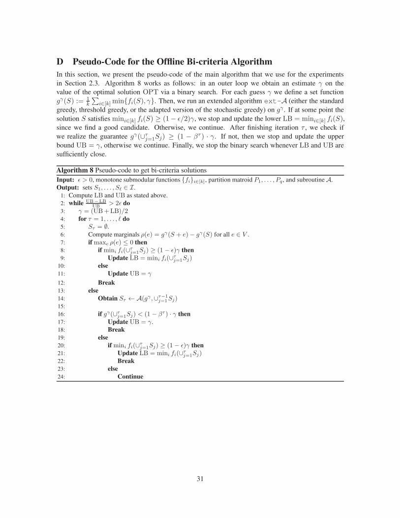
D Pseudo-Code for the Offline Bi-criteria Algorithm

In this section, we present the pseudo-code of the main algorithm that we use for the experimentsin Section 2.3. Algorithm 8 works as follows: in an outer loop we obtain an estimate γ on thevalue of the optimal solution OPT via a binary search. For each guess γ we define a set functiongγ(S) := 1

k

∑

i∈[k]min{fi(S), γ}. Then, we run an extended algorithm ext-A (either the standardgreedy, threshold greedy, or the adapted version of the stochastic greedy) on gγ . If at some point thesolution S satisfies mini∈[k] fi(S) ≥ (1− ǫ/2)γ, we stop and update the lower LB = mini∈[k] fi(S),since we find a good candidate. Otherwise, we continue. After finishing iteration τ , we check ifwe realize the guarantee gγ(∪τj=1Sj) ≥ (1 − βτ ) · γ. If not, then we stop and update the upperbound UB = γ, otherwise we continue. Finally, we stop the binary search whenever LB and UB aresufficiently close.

Algorithm 8 Pseudo-code to get bi-criteria solutionsInput: ǫ > 0, monotone submodular functions {fi}i∈[k], partition matroid P1, . . . , Pq , and subroutineA.Output: sets S1, . . . , Sℓ ∈ I.

1: Compute LB and UB as stated above.2: while UB−LB

UB > 2ǫ do

3: γ = (UB+LB)/24: for τ = 1, . . . , ℓ do

5: Sτ = ∅.6: Compute marginals ρ(e) = gγ(S + e)− gγ(S) for all e ∈ V .7: if maxe ρ(e) ≤ 0 then

8: if mini fi(∪τj=1Sj) ≥ (1 − ǫ)γ then

9: Update LB = mini fi(∪τj=1Sj)10: else

11: Update UB = γ

12: Break

13: else

14: Obtain Sτ ← A(gγ ,∪τ−1j=1Sj)

15:16: if gγ(∪τj=1Sj) < (1 − βτ ) · γ then

17: Update UB = γ.18: Break

19: else

20: if mini fi(∪τj=1Sj) ≥ (1− ǫ)γ then

21: Update LB = mini fi(∪τj=1Sj)22: Break

23: else

24: Continue

31

Structured Robust Submodular Maximization - arXiv

Documents

Transcript of Structured Robust Submodular Maximization - arXiv