gamm header will be provided by the publisher

Structured Eigenvalue Problems

Heike Fassbender∗1 and Daniel Kressner∗∗2

1 Institut Computational Mathematics, TU Braunschweig, D-38023 Braunschweig2 Department of Mathematics, University of Zagreb, Croatia; Department of Computing Sci-

ence, Umea University, Sweden

Received 15 April 2005

Key words Structured matrix, eigenvalue, invariant subspace, numerical methods, software.

MSC (2000) 65-F15

Most eigenvalue problems arising in practice are known to be structured. Structure is oftenintroduced by discretization and linearization techniques but may also be a consequence ofproperties induced by the original problem. Preserving this structure can help preserve phys-ically relevant symmetries in the eigenvalues of the matrix and may improve the accuracyand efficiency of an eigenvalue computation. The purpose of this brief survey is to highlightthese facts for some common matrix structures. This includes a treatment of rather generalconcepts such as structured condition numbers and backward errors as well as an overview ofalgorithms and applications for several matrix classes including symmetric, skew-symmetric,persymmetric, block cyclic, Hamiltonian, symplectic and orthogonal matrices.

Copyright line will be provided by the publisher

1 Introduction

This survey is concerned with computing eigenvalues, eigenvectors and invariant subspacesof a structured square matrix A. In the scope of this paper, an n×n matrix A is considered tobe structured if its n2 entries depend on less than n2 parameters.

It usually takes a long process of simplifications, linearizations and discretizations beforeone comes up with the problem of computing the eigenvalues or invariant subspaces of amatrix. These techniques typically lead to highly structured matrix representations, which,for example, may contain redundancy or inherit some physical properties from the originalproblem. As a simple example, let us consider a quadratic eigenvalue problem of the form

(λ2In + λC + K)x = 0, (1)

where C ∈ Rn×n is skew-symmetric (C = −CT ), K ∈ Rn×n is symmetric (K = KT ),and In denotes the n × n identity matrix. Eigenvalue problems of this type arise, e.g., fromgyroscopic systems [96, 117] or Maxwell equations [108]; they have the physically relevantproperty that all eigenvalues appear in quadruples {λ,−λ, λ,−λ}, i.e., the spectrum is sym-metric with respect to the real and imaginary axes. Linearization turns (1) into a matrix

∗ e-mail: h.fassbender@tu-bs.de∗∗ Corresponding author: e-mail: kressner@cs.umu.se.

Copyright line will be provided by the publisher

2 H. Fassbender and D. Kressner: Structured Eigenvalue Problems

−20 −10 0 10 20−200

−150

−100

−50

0

50

100

150

200

−20 −10 0 10 20−200

−150

−100

−50

0

50

100

150

200

Fig. 1 Eigenvalues (’·’) and approximate eigenvalues (’×’) computed by a standard Arnoldi method(left picture) and by a structure-preserving Arnoldi method (right picture).

eigenvalue problem, e.g., the eigenvalues of (1) can be obtained from the eigenvalues of thematrix

A =

[

− 12C 1

4C2 − KIn − 1

2C

]

. (2)

This 2n × 2n matrix is structured, its 4n2 entries depend only on the n2 entries necessary todefine C and K. The matrix A has the particular property that it is a Hamiltonian matrix, i.e.,A is a two-by-two block matrix of the form

[

B GQ −BT

]

, G = GT , Q = QT , B, G, Q ∈ Rn×n.

Considering A to be Hamiltonian does not capture all the structure present in A but it capturesan essential part: The spectrum of any Hamiltonian matrix is symmetric with respect to thereal and and imaginary axes. Hence, numerical methods that take this structure into accountare capable to preserve the eigenvalue pairings of the original eigenvalue problem (1), despitethe presence of roundoff and other approximation errors.

Figure 1, which displays the eigenvalues of a quadratic eigenvalue problem (1) stemmingfrom a discretized Maxwell equation [108], illustrates this fact. The exact eigenvalues are rep-resented by grey dots in each plot,; one can clearly see the eigenvalue pairing {λ,−λ, λ,−λ},for complex eigenvalues with nonzero real part and {λ,−λ} for real and purely imaginaryeigenvalues. Eigenvalue approximations (denoted by black crosses) have been computed withtwo different types of Arnoldi methods (a standard approach for computing approximations tosome eigenvalues of large sparse matrices): in the plot on the left hand side the eigenvalue ap-proximations were obtained from a few iterations of the standard Arnoldi method [51] whilethe ones in the plot on the right hand side were obtained from the same number of iterationsof an Arnoldi method that takes Hamiltonian structures into account, see [96] and Section 3.7.It is particularly remarkable that the latter method produces not only pairs of eigenvalue ap-proximations, but also purely imaginary approximations to purely imaginary eigenvalues.

Besides the preservation of such eigenvalue symmetries, there are several other benefits tobe gained from using structure-preserving algorithms in place of general-purpose algorithms

Copyright line will be provided by the publisher

gamm header will be provided by the publisher 3

for computing eigenvalues. These benefits include reduced computational time and improvedeigenvalue/eigenvector accuracy.

This paper is organized as follows. In Section 2, we will present several general conceptsrelated to (structured) eigenvalue problems. To be more specific, Section 2.1 provides a sum-mary of common algorithms for solving eigenvalue problems while Section 2.2 discusses theefficiency gains to be expected from exploiting structure. Sections 2.3 and 2.4 are concernedwith (structured) backward stability and condition numbers; both concepts are closely relatedto the accuracy of eigenvalues in finite-precision arithmetic. Section 3 treats several classes ofmatrices individually: symmetric, skew-symmetric, persymmetric, block cyclic, Hamiltonian,orthogonal, and others. This treatment includes a brief overview of existing algorithms andapplications for each of these structures.

1.1 Preliminaries

The eigenvalues of a real or complex n×n matrix A are the roots of its characteristic polyno-mial det(A − λI). Since the degree of the characteristic polynomial equals n, the dimensionof A, it has n roots, so A has n eigenvalues. The eigenvalues may be real or complex, evenif A is real (in that case, complex eigenvalues appear in pairs {λ, λ}. The set of all eigen-values will be denoted by λ(A). A nonzero vector x ∈ Cn is called an (right) eigenvectorof A if it satisfies Ax = λx for some λ ∈ λ(A). A nonzero vector y ∈ Cn is called aleft eigenvector if it satisfies yHA = λyH , where yH denotes the Hermitian transpose of y.Spaces spanned by eigenvectors remain invariant under multiplication by A, in the sense thatspan{Ax} = span{λx} ⊆ span{x}. This concept generalizes to higher-dimensional spaces.A linear subspace X ⊂ Cn with Ax ∈ X for all x ∈ X is called an invariant subspace of A.

If n > 4 there is no general closed formula for the roots of a polynomial in terms of itscoefficients, and therefore one has to resort to a numerical technique in order to compute theroots by successive approximation. A further difficulty is that the roots may be very sensitiveto small changes in the coefficients of the polynomial, and the effect of rounding errors in theconstruction of the characteristic polynomial is usually catastrophic (see Section 2.1 for anexample). Numerically more reliable methods are obtained from the following observation.Eigenvalues and invariant subspaces can be easily obtained from the Schur decomposition ofA: There is always a unitary matrix U (UHU = UUH = I) such that

T = UHAU

is upper triangular, that is, tij = 0 for i > j. As λ(A) equals λ(T ), the eigenvalues of A canbe read off from the diagonal entries of T . Moreover, if we partition U = [X, X⊥], whereX ∈ Cn×k for some 1 ≤ k < n, then we may rewrite the relation AU = TU as

A[X, X⊥] = [X, X⊥]

[

T11 T12

0 T22

]

, T11 ∈ Ck×k , T22 ∈ C

(n−k)×(n−k). (3)

This shows that AX = XT11, i.e., the columns of X form an orthonormal basis for theinvariant subspace X belonging to λ(T11). Bases for invariant subspaces belonging to othereigenvalues can be obtained by changing the order of the eigenvalues on the diagonal ofT [51].

In case the matrix A is real, one would like to restrict the equivalence transformation whichreveals the eigenvalues and corresponding invariant subspaces to a real transformation. As A

Copyright line will be provided by the publisher

4 H. Fassbender and D. Kressner: Structured Eigenvalue Problems

may have complex eigenvalues, a reduction to the above introduced Schur form is no longerpossible. We must lower our expectations and be content with the calculation of an alternativedecomposition known as the real Schur decomposition: There always exists an orthogonalmatrix Q (QT Q = QQT = I) such that QT AQ = TR is upper quasi-triangular, that is, TR isblock upper triangular with either 1 × 1 or 2 × 2 diagonal blocks. Each 2 × 2 diagonal blockcorresponds to a pair of complex conjugate eigenvalues.

2 General Concepts

In this section, we briefly summarize some general concepts related to general and structuredeigenvalue computations.

2.1 Algorithms

Algorithms for solving structured eigenvalue problems are often extensions or special casesof existing algorithms for solving the general, unstructured eigenvalue problem. One canroughly divide these algorithms into direct methods and iterative methods.

Direct methods aim at computing all eigenvalues and (optionally) eigenvectors/invariantsubspaces of a matrix A. The most widely used direct method for general nonsymmetric ma-trices is the QR algorithm [51]. This algorithm, which is behind the MATLAB [93] commandeig, computes a sequence of matrix decompositions converging to a complete Schur form ofA by implicitly applying a QR decomposition in each iteration. Jacobi-like methods [45, 112]apply a sweep of elementary transformations, such as Givens rotations, in each iteration. Theyare well-suited for parallel computation but their slow speed of convergence makes them ofteninferior to the QR algorithm unless there is some special structure in A, e.g., A is symmetricor close to being upper triangular. Moreover, Jacobi’s method can sometimes compute tinyeigenvalues much more accurately than other methods [41].

Iterative methods aim at computing a selected set of eigenvalues and (optionally) the eigen-vectors/invariant subspaces belonging to these eigenvalues. The most widely known iterativemethod is probably the power method [51]. Starting from some random vector v, one con-structs a sequence v, Av, A2v, A3v, . . . by repeated matrix-vector multiplication. This se-quence converges to an eigenvector belonging to the dominant eigenvalue (i.e., the eigenvalueof largest magnitude), provided that there is only one such eigenvalue. Besides being inca-pable of obtaining several eigenvalues or eigenvectors, the power method may also suffer fromvery slow convergence in the presence of several nearly dominant eigenvalues. To find othereigenvalues and eigenvectors, the power method can be applied to (A− σI)−1 for some shiftσ, an algorithm called inverse iteration. The largest eigenvalue of (A − σI)−1 is 1/(λi − σ)where λi is the closest eigenvalue of A to σ, so that one can choose which eigenvalues to findby choosing σ.

The Arnoldi method [5, 51] achieves faster convergence by considering not only the lastiterate of the power method but the whole space spanned by all previous iterates, the so calledKrylov subspace Kk(A, v) := span{v, Av, . . . , Ak−1v}. Using Krylov subspaces also givesthe flexibility to approximate several eigenvalues and the associated invariant subspaces. Theincreased memory requirements of the Arnoldi method can be limited by employing restartingstrategies, see, e.g., [110]. This leads to the implicitly restarted Arnoldi algorithm [85] (IRA),which forms the basis of MATLAB’s eigs.

Copyright line will be provided by the publisher

gamm header will be provided by the publisher 5

0 5 10 15 20 25−2

−1.5

−1

−0.5

0

0.5

1

1.5

2

Fig. 2 Computed roots (’×’) of the polynomial (λ− 1)(λ− 2) · · · (λ− 25), after its coefficients havebeen stored in double-precision.

A different class of iterative methods is obtained by applying Newton’s method to a systemof nonlinear equations satisfied by an eigenvalue/eigenvector pair (λ, x). One such system isgiven by

f(λ, x) :=

[

Ax − λxwHx − 1

]

= 0,

where w is a suitably chosen vector. It turns out that Newton’s method applied to this systemis equivalent to inverse iteration, see also [95] for more details. The Jacobi-Davidson method(see the review in the present volume of this journal or [5, 109]) is a closely related Newton-like method, but so far little is known about adapting this method to structured eigenvalueproblems. There are other functions f that may be used, but not all of them lead to practicallyuseful methods for computing eigenvalues. For example, using p(λ) = det(λI − A) by ex-plicitely constructing the coefficients of the polynomial p(λ) is generally not advisable. Often,already storing these coefficients in finite-precision arithmetic leads to an unacceptably higherror in the eigenvalues; leave alone any other roundoff error implied by the typically wildlyvarying magnitudes. Figure 2, which goes back to an example by Wilkinson [134], illustratesthis effect. However, it should be mentioned that iterative methods based on p(λ) are suitablefor some classes of matrices such as tridiagonal matrices, but great care in representing p(λ)must be taken, see [13] and the references therein.

2.2 Efficiency

Direct methods generally require O(n3) computational time to compute the eigenvalues of ageneral n × n matrix. The fact that a structured matrix depends on less than n2 parametersgives rise to the hope that an algorithm taking advantage of the structure may require lesseffort than a general-purpose algorithm. For example, the QR algorithm applied to a symmet-ric matrix requires roughly 10% of the floating point operations (flops) required by the samealgorithm applied to a general matrix [51]. For other structures, such as skew-Hamiltonianand Hamiltonian matrices, this figure can be less dramatic [9]. Moreover, in view of recentprogress made in improving the performance of general-purpose algorithms [21, 22], it may

Copyright line will be provided by the publisher

6 H. Fassbender and D. Kressner: Structured Eigenvalue Problems

require considerable implementation efforts to turn this reduction of flops into an actual re-duction of computational time.

The convergence of an iterative method strongly depends on the properties of the matrix Aand the subset of eigenvalues to be computed, which makes the needed computational effortrather difficult to predict. For example, methods based on Krylov subspaces require in eachiteration a matrix-vector multiplication, which can take up to 2n2 flops. This figure mayreduce significantly for a structured matrix A, e.g., to roughly twice the number of nonzeroentries for sparse matrices. Some structures, such as skew-Hamiltonian and persymmetricmatrices [96, 125], induce some additional structure in the Krylov subspace making it possibleto reduce the computational effort even further.

2.3 Backward error and backward stability

Any numerical method for computing eigenvalues is affected by round-off errors due to thelimitations of finite-precision arithmetic. Already representing the entries of a matrix A indouble-precision generally causes a relative error of about 10−16. Unless some further in-formation is available, the best we can therefore expect from our numerical method is thatit computes the exact eigenvalues of a slightly perturbed matrix A + E, where ‖E‖F (theFrobenius norm of E) is not much greater than 10−16 × ‖A‖F . A numerical method satis-fying this property is called (numerically) backward stable. Methods known to be backwardstable include the QR algorithm, most Jacobi-like methods, the power method, the Arnoldimethod, IRA, and many of the better Newton-like methods.

A simple way to check backward stability is to compute the residual r = Ax − λx of acomputed eigenvalue/eigenvector pair (λ, x) with ‖x‖2 = 1. Then (λ, x) is an exact eigenpairof the perturbed matrix A− rxH and the backward error is consequently given by ‖rxH‖F =

‖r‖2. If only λ is available then a suitable backward error is given by σmin(A − λI), whichcoincides with the 2-norm of the smallest perturbation E such that λ is an eigenvalue of A+E.(Here, σmin denotes the smallest singular value of a matrix.)

The notion of structured backward error not only requires (λ, x) to be an exact eigenpairof A + E but also requires A + E to stay within the considered class of structured matrices.For example, if A is symmetric then a suitable symmetric E is given by E = −(rxT + xrT −(rT x)xxT ). Since ‖r‖2 ≤ ‖E‖2 ≤ ‖r‖2/

√2, this implies that the structured backward error

with respect to symmetric matrices is rather close to the standard backward error. This is notfor all structures the case, see [116] for more details. Depending on the point of view, theproblem of finding the structured backward error can also be regarded as a structured inverseeigenvalue problem [36] or computing the smallest structured singular value [66, 73].

A numerical method is called strongly backward stable if the computed eigenpairs satisfysmall structured backward errors [24]. Strong backward stability implies backward stability,but the converse is generally not true.

2.4 Condition numbers and pseudospectra

Knowing that a computed eigenvalue satisfies a small (structured) backward error does notnecessarily admit conclusions about the accuracy of this eigenvalue. This also depends on the

Copyright line will be provided by the publisher

gamm header will be provided by the publisher 7

ε = 0.6 ε = 0.4 ε = 0.2

Fig. 3 Unstructured pseudospectra of the matrix A in (6) for different perturbation levels ε.

eigenvalue condition number κ(λ), which is formally defined as follows:

κ(λ) := limε→0

1

εsup{|λ − λ| : E ∈ C

n×n, ‖E‖2 ≤ ε}, (4)

where λ is the eigenvalue of the perturbed matrix A + E closest to λ. In other words, κ(λ)measures the worst-case first order influence of a perturbation E on the accuracy of λ. If κ(λ)is large, then λ is said to be ill-conditioned. Eigenvalues with small condition number are saidto be well-conditioned.

The definition (4) readily implies |λ − λ| / κ(λ)‖E‖2. Thus, a backward stable methodattains high accuracy for fairly well-conditioned eigenvalues. If λ is a simple eigenvalue,i.e., λ is a simple root of det(λI − A), then κ(λ) = 1/|yHx| with x and y being rightand left eigenvectors belonging to λ normalized such that ‖x‖2 = ‖y‖2 = 1 [51]. Forany normal matrix N (that is NHN = NNH) there exists a unitary matrix Q such thatQHNQ = diag(λ1, . . . , λn) is diagonal. Hence, Nqj = λjqj and qH

j N = qHj λj . Its every

right eigenvector is also a left eigenvector belonging to the same eigenvalue and κ(λ) = 1 forall its eigenvalues. Hence, eigenvalues of normal matrices are well-conditioned.

Pseudospectra provide more detailed information on the behavior of eigenvalues underperturbations [118]. For a given perturbation level ε > 0, the pseudospectrum Λε(A) of A isthe union of the eigenvalues of all perturbed matrices A + E with ‖E‖2 ≤ ε:

Λε(A) :=⋃

{Λ(A + E) : E ∈ Cn×n, ‖E‖2 ≤ ε}. (5)

Figure 3 displays pseudospectra for the matrix

A =

2 1 2−1 2 2

0 0 0

. (6)

Provided that all eigenvalues are simple, the pseudospectrum approaches, as ε tends to zero,discs around the eigenvalues and the radii of these discs divided by ε coincide with the corre-sponding eigenvalue condition numbers, see, e.g., [73].

Copyright line will be provided by the publisher

8 H. Fassbender and D. Kressner: Structured Eigenvalue Problems

ε = 0.6 ε = 0.4 ε = 0.2

Fig. 4 Real pseudospectra of the matrix A in (6) for different perturbation levels ε.

This is no longer true if we only admit structured perturbations in (5), i.e., matrices E thatbelong to a certain matrix class struct. The corresponding structured pseudospectrum Λstruct

ε

may approach completely different geometrical shapes [66, 73]. For example, if we allow forreal perturbations only, then struct ≡ R

n×n. ΛRn×n

ε is known to approach ellipses. This isdemonstrated in Figure 4 (a line can be regarded as a degenerated ellipse). The larger halfdiameters of these ellipses divided by ε yield the structured eigenvalue condition numbers,formally defined as

κstruct(λ) := limε→0

1

εsup{|λ − λ| : E ∈ struct, ‖E‖2 ≤ ε}. (7)

It turns out that κRn×n

(λ) ≥ κ(λ)/√

2, see [30]. Since κstruct(λ) ≤ κ(λ) holds for any struct,this implies that there is no significant difference between κR

n×n

(λ) and κ(λ). Surprisingly,the same statement holds for a variety of other structures [18, 55, 74, 107], see also Section 3.Note that (7) implies |λ − λ| / κstruct(λ)‖E‖2 for all E ∈ struct. Explicit expressions forκstruct(λ) have been derived in [64], provided that struct is a linear matrix space.

Defining an appropriate condition number κ(X ) for an invariant subspace X of A is morecomplicated due to the fact that we have to work with subspaces and rely on a meaning-ful notion of distances between subspaces. Such a notion is provided by the canonical an-gles [111, 113] and the resulting κ(X ) can be interpreted as follows. Let the columns of X

form an orthonormal basis for X . Then there is a matrix X such that the columns of X forma basis for an invariant subspace X of the slightly perturbed matrix A + E and

‖X − X‖F / κ(X )‖E‖F

for all E ∈ Cn×n. A (possibly smaller) κstruct(X ) is similarly defined and yields the samebound for all E restricted to struct. Structured condition numbers for eigenvectors and in-variant subspaces have been studied in [31, 64, 68, 77, 79, 114]. The (structured) perturbationanalysis of quadratic matrix equations is a closely related area, which is comprehensivelytreated in [76, 115].

Copyright line will be provided by the publisher

gamm header will be provided by the publisher 9

3 More on Some Structures

In this section, we aim to provide a brief discussion on selected aspects of some commonmatrix structures.

3.1 Sparsity and related structures

Sparsity is probably the most ubiquitous structure in (numerical) linear algebra. While asparse matrix cannot be expected to have any particular eigenvalue or eigenvector properties,it always admits the efficient calculation of its eigenvalues and eigenvectors [5], see alsoSection 2.2.

In [101], it was shown that if struct denotes all matrices having an assigned sparsity patternthen the corresponding structured eigenvalue condition number equals ‖(yxH)|struct‖F /|yHx|,where (yxH)|struct means the restriction of the rank-one matrix yxH to the sparsity structureof struct. For example if the perturbation is upper triangular then (yxH)|struct is the uppertriangular part of yxH .

No methods are known to be strongly backward stable for an arbitrary sparsity structurestruct. Hence, it is generally difficult to achieve accuracy gains promised by a small value of‖(yxH)|struct‖F .

3.2 Symmetric matrices

Probably the two most fundamental properties of a symmetric matrix A ∈ Rn×n, A = AT , arethat every eigenvalue is real and every right eigenvector is also a left eigenvector belongingto the same eigenvalue. Both facts immediately follow from the observation that a Schurdecomposition of A always takes the form QT AQ = diag(λ1, . . . , λn).

It is simple to show that the structured eigenvalue and invariant subspace condition numbersare equal to the corresponding unstructured condition numbers, i.e., κsymm(λ) = κ(λ) = 1and

κsymm(X ) = κ(X ) =1

min{|µ − λ| : λ ∈ Λ1, µ ∈ Λ2},

where X is a simple invariant subspace belonging to an eigenvalue subset Λ1 ⊂ λ(A), andΛ2 = λ(A)\Λ1. Moreover, many numerical methods, such as QR, Arnoldi and Jacobi-Davidson, automatically preserve symmetric matrices and are strongly backward stable.

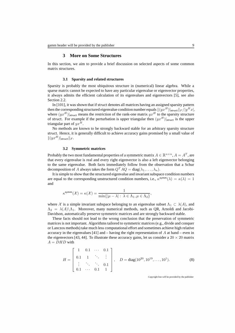
These facts should not lead to the wrong conclusion that the preservation of symmetricmatrices is not important. Algorithms tailored to symmetric matrices (e.g., divide and conqueror Lanczos methods) take much less computational effort and sometimes achieve high relativeaccuracy in the eigenvalues [41] and – having the right representation of A at hand – even inthe eigenvectors [43, 44]. To illustrate these accuracy gains, let us consider a 20 × 20 matrixA = DHD with

H =

1 0.1 · · · 0.1

0.1 1. . .

......

. . .. . . 0.1

0.1 · · · 0.1 1

, D = diag(1020, 1019, . . . , 101). (8)

Copyright line will be provided by the publisher

10 H. Fassbender and D. Kressner: Structured Eigenvalue Problems

2 4 6 8 10 12 14 16 18 2010

−20

10−15

10−10

10−5

100

eigenvalues

rela

tive

erro

rQR algorithm

2 4 6 8 10 12 14 16 18 2010

−17

10−16

10−15

10−14

eigenvalues

rela

tive

erro

r

Jacobi algorithm

Fig. 5 Relative errors |λ−λ|/λ for the eigenvalues of the matrix A = DHD as defined in (8) computedby the QR algorithm and by the Jacobi algorithm.

From Figure 5 it can be concluded that the Jacobi algorithm computes all eigenvalues of Awith high relative accuracy while the QR algorithm fails to achieve this goal.

Besides the well-known algorithms for symmetric eigenproblems such as the QR algo-rithm, the Lanczos algorithm (a Krylov subspace method tailored for symmetric matrices)and the Jacobi method, which are discussed in most basic books on numerical methods (see,e.g., [51, 131, 40]), there are a number of more recent developments. For example, a divide-and-conquer algorithm was first introduced in 1981 [39]. Its quite subtle implementation wasonly discovered ten years later [58]. The algorithm is one of the fastest now available forcomputing all eigenvalues and all eigenvectors. Bisection can be used to find just a subsetof the eigenvalues of a symmetric tridiagonal matrix, e.g., those in the interval [a, b]. If onlyk � n eigenvalues are required, bisection can be much faster then QR. Inverse iteration canthen be used to independently compute the corresponding eigenvectors. The numerical diffi-culties associated with that approach have recently be resolved [42, 43, 44]. Of course, therea symmetric version of the Jacobi-Davidson algorithm (see the review in the present volumeof this journal or [5, 109]).

An overview of all developments related to symmetric eigenvalue problems is far beyondthe scope of this survey; we refer to [37, 40, 103] for introductions to this flourishing branchof eigenvalue computation.

3.3 Skew-symmetric matrices

Any eigenvalue of a skew-symmetric matrix A ∈ Rn×n, A = −AT , is purely imaginary.If n is odd then there is at least one zero eigenvalue. As for symmetric matrices, any righteigenvector is also a left eigenvector belonging to the same eigenvalue (this is true for anynormal matrix). The real Schur form of A takes the form

QT AQ =

[

0 α1

−α1 0

]

⊕ · · · ⊕[

0 αk

−αk 0

]

⊕ 0 ⊕ · · · ⊕ 0.

for some real scalars α1, . . . , αk 6= 0.

Copyright line will be provided by the publisher

gamm header will be provided by the publisher 11

While the structured condition number for a nonzero eigenvalue always satisfies κskew(λ) =κ(λ) = 1, we have for a simple zero eigenvalue κskew(0) = 0 but κ(0) = 1 [107]. Again, thereis nothing to be gained for an invariant subspace X ; it is simple to show κskew(X ) = κ(X ).

Skew-symmetric matrices have received much less attention than symmetric matrices,probably due to the fact that skew-symmetry plays a less important role in applications. Again,the QR and the Arnoldi algorithm automatically preserve skew-symmetric matrices. Variantsof the QR algorithm tailored to skew-symmetric matrices have been discussed in [72, 128].Jacobi-like algorithms for skew-symmetric matrices and other Lie algebras have been devel-oped and analyzed in [59, 60, 61, 75, 102, 106, 133].

3.4 Persymmetric matrices

A real 2n × 2n matrix A is called persymmetric if it is symmetric with respect to the anti-diagonal. E.g., A takes the following form for n = 2:

A =

a11 a12 a13 a14

a21 a22 a23 a13

a31 a12 a22 a12

a41 a31 a21 a11

.

If we additionally assume A to be symmetric, then we can write

A =

[

A11 A12

AT12 FnAT

11Fn

]

,

where Fn denotes the n×n flip matrix, i.e., Fn has ones on the anti-diagonal and zeros every-where else. Note that A is also a centrosymmetric matrix since A = F2nAF2n. A practicallyrelevant example of such a matrix is the Gramian of a set of frequency exponentials {e±ıλkt},which plays a role in the control of mechanical and electric vibrations [105]. Employing the

orthogonal matrix U = 1√2

[

I−Fn

Fn

I

]

we have

UT AU =

[

A11 − A12Fn 00 FnA11Fn + FnA12

]

, (9)

where we used the symmetry of A11 and the persymmetry of A12. This is a popular trickwhen dealing with centrosymmetric matrices [132]. (A similar but technically slightly morecomplicated trick can be used if A has odd dimension.) Thus,

λ(A) = λ(A11 − A12Fn) ∪ λ(A11 + A12Fn).

Perhaps more importantly, if these two eigenvalue sets are disjoint then any eigenvector be-longing to λ(A11 − A12Fn) takes the form

x = U

[

x0

]

=

[

x−Fnx

]

for some x ∈ Rn. This property of x is sometimes called center-skew-symmetry. Analo-gously, any eigenvector belonging to λ(A11 + A12Fn) is center-symmetric. While the struc-tured and unstructured eigenvalue condition numbers for symmetric persymmetric matrices

Copyright line will be provided by the publisher

12 H. Fassbender and D. Kressner: Structured Eigenvalue Problems

are the same [74, 107], there can be a significant difference in the invariant subspace conditionnumbers. With respect to structured perturbations, the separation between λ(A11 − A12Fn)and λ(A11 + A12Fn), which can be arbitrarily small, does not play any role for invariantsubspaces belonging to eigenvalues from one of the two eigenvalue sets [31]. It can thus beimportant to retain the symmetry structure of the eigenvectors in finite-precision arithmetic.Krylov subspace methods achieve this goal automatically if the starting vector is chosen tobe center-symmetric (or center-skew-symmetric). This property has been used in [125] toconstruct a structure-preserving Lanczos process. Efficient algorithms for performing matrix-vector products with centrosymmetric matrices have been investigated in [48, 97, 100].

We now briefly consider a persymmetric and skew-symmetric matrix A,

A =

[

A11 A12

−AT12 FnAT

11Fn

]

.

Again, the orthogonal matrix U can be used to reduce A:

UT AU =

[

0 A11Fn + A12

FnA11 − AT12 0

]

.

Hence, the eigenvalues of A are the positive and negative square roots of the eigenvalues ofthe matrix product (A11Fn + A12)(FnA11 − AT

12), see also [105].Structure-preserving Jacobi algorithms for symmetric persymmetric and skew-symmetric

persymmetric matrices have been recently developed in [90].

3.5 Product eigenvalue problems and block cyclic matrices

The task of computing the eigenvalues of a matrix product arises from various applications insystems and control theory, see, e.g., [7, 23, 89, 123]. Moreover, it has been recently shownthat many structured eigenvalue problems can be viewed as particular instances of the producteigenvalue problem [130].

For simplicity, let us consider computing the eigenvalues of an n × n product of threematrices only: Π = ABC. At first sight, such an eigenvalue problem does not match thedefinition of a structured eigenvalue problem stated in the beginning of this survey; Π is ann × n matrix but depends on the 3n2 entries defining its factors A, B, C. However, anyproduct eigenvalue problem can be equivalently seen as an embedded block cyclic structuredeigenvalue problem:

A =

0 0 CB 0 00 A 0

.

The fact that A3 is a block diagonal matrix with diagonal entries CAB, BCA, ABC im-plies that λ is an eigenvalue of A if and only if λ3 is an eigenvalue of ABC (which hasthe same eigenvalues as CAB and BCA). Also, any invariant subspace of ABC can berelated to an invariant subspace of A [87]. This connection admits the application of struc-tured perturbation results to obtain factor-wise perturbation results for the product eigenvalueproblem [11, 35, 81, 86].

Copyright line will be provided by the publisher

gamm header will be provided by the publisher 13

The essential key to develop numerically stable algorithms for solving a product eigen-value problem is to avoid the explicit computation of the matrix product. The periodic QRalgorithm [17, 63, 119] is a strongly backward stable method for computing eigenvalues andinvariant subspaces of A, which in turn implies factor-wise backward stability for computingeigenvalues and invariant subspaces of Π. In [78], it has been shown numerically equivalent tothe standard QR algorithm applied to a permuted version of A. Methods for solving producteigenvalue problems with large and (possibly) sparse factors can be found in [80, 88]. Usingthese methods instead of applying a standard method to Π often results in higher accuracyfor the computed eigenvalues, especially for those of small magnitude. This well-appreciatedadvantage has driven the development of many reliable algorithms for solving instances ofthe product eigenvalue problem, such as the Golub-Reinsch algorithm for the singular valuedecomposition [50] or the QZ algorithm for the generalized eigenvalue problem [99].

3.6 Orthogonal matrices

All the eigenvalues of a real orthogonal matrix Q lie on the unit circle. Moreover, as orthogo-nality implies normality, any right eigenvector is also a left eigenvector belonging to the sameeigenvalue. Orthogonal eigenvalue problems have a number of applications in digital signalprocessing, see [1, 2] for an overview.

The set of orthogonal matrices orth = {A : AT A = I} forms a smooth manifold, and thetangent space of orth at A is given by {AH : H ∈ skew}. By the results in [74] this implies

κorth(λ) = sup{|xHAHx| : H ∈ skew, ‖AH‖2 = 1}= sup{|xHHx| : H ∈ skew, ‖H‖2 = 1}.

Hence, if λ = ±1 then x can be chosen to be real which implies xT Hx = 0 for all x andconsequently κorth(λ) = 0, provided that λ is simple. Similarly, if λ is complex, we haveκorth(λ) = κ(λ) = 1 and hence corth

2 (λ) = 1. A more general perturbation analysis oforthogonal and unitary eigenvalue problems, based on the Cayley transform, can be foundin [16].

Once again, the QR algorithm automatically preserves orthogonal matrices. To make itwork (efficiently), it is important to take the fact that the underlying matrix is orthogonalinto account. A careful choice of shifts can lead to cubic convergence or even ensure globalconvergence [46, 126, 127]. Even better, an orthogonal (or unitary) Hessenberg matrix can berepresented by O(n) so called Schur parameters [52, 27]. This makes it possible to implementthe QR algorithm very efficiently [53]; for an extension to unitary and orthogonal matrixpairs, see [25]. In [54], a divide and conquer approach for unitary Hessenberg matrices wasproposed, based on the methodology of Cuppen’s divide and conquer approach for symmetrictridiagonal matrices [38]. Krylov subspace methods for orthogonal and unitary matrices havebeen developed and analyzed in [15, 26, 62, 70, 71].

3.7 Hamiltonian matrices

As already mentioned in the introduction, one of the most remarkable properties of a Hamil-tonian matrix

H =

[

A GQ −AT

]

, G = GT , Q = QT ,

Copyright line will be provided by the publisher

14 H. Fassbender and D. Kressner: Structured Eigenvalue Problems

is that its eigenvalues always occur in pairs {λ,−λ}, if λ ∈ R ∪ ıR, or in quadruples{λ,−λ, λ,−λ}, if λ ∈ C\(R ∪ ıR). Hamiltonian matrices arise in applications related tolinear control theory for continuous-time systems [6] and quadratic eigenvalue problems [96,117], to name only a few. Deciding whether a certain Hamiltonian matrix has purely imagi-nary eigenvalues is the most critical step in algorithms for computing the stability radius of amatrix or the H∞ norm of a linear time-invariant system, see, e.g., [20, 29].

The described eigenvalue pairings often reflect important properties of the underlying ap-plication and should thus be preserved in finite-precision arithmetic. QR-like algorithms thatachieve this goal have been developed in [10, 28, 120] while Krylov subspace methods tailoredto Hamiltonian matrices can be found in [8, 9, 49, 96, 129]. An efficient strongly backwardstable method for computing invariant subspaces of H has recently been proposed in [34].

Concerning structured perturbation results for Hamiltonian matrices, see [31, 74, 77, 116]and the references therein. It turns out that there is no or little difference between κ(λ) andκHamil(λ), the (structured) eigenvalue condition numbers. Also, κ(X ) and κHamil(X ) are equalfor the important case that X is the invariant subspace belonging to all eigenvalues in the openleft half plane.

There is much more to be said about Hamiltonian eigenvalue problems, see [9] for a recentsurvey.

3.8 Symplectic matrices

A matrix M is called symplectic iff

MJMT = J,

or equivalently, MT JM = J, where

J =

[

0 I−I 0

]

.

The symplectic matrices form a group under multiplication. The eigenvalues of symplecticmatrices occur in reciprocal pairs: If λ is an eigenvalue of M with right eigenvector x, thenλ−1 is an eigenvalue of M with left eigenvector (Jx)T . The computation of eigenvaluesand eigenvectors of such matrices is an important task in applications like the discrete linear-quadratic regulator problem, discrete Kalman filtering, the solution of discrete-time algebraicRiccati equations and certain large, sparse quadratic eigenvalue problems. See, e.g., [82, 84,94, 96] for applications and further references. Symplectic matrices also occur when solvinglinear Hamiltonian difference systems [14].

Note that a Calyley transform turns a symplectic matrix into a Hamiltonian one and viceversa. This explains the close resemblence of the spectra of Hamiltonian and symplectic ma-trices. Moreover, every Hamiltonian matrix H satisfies HJ = (HJ)T . Unfortunately, theHamiltonian and the symplectic eigenproblems are (despite common believe) quite different.The symplectic eigenproblem is much more difficult than the Hamiltonian one. The relationbetween the two eigenproblems is best described by comparing it with the relation betweensymmetric and orthogonal eigenproblems or the Hermitian and unitary eigenproblems. In allthese cases, the underlying algebraic structures are an algebra and a group acting on this alge-bra. For the algebra (Hamiltonian, symmetric, Hermitian matrices), the structure is explicit,

Copyright line will be provided by the publisher

gamm header will be provided by the publisher 15

i.e., can be read off the matrix by viewing it. In contrast, the structure of a matrix contained ina group (symplectic, orthogonal, unitary matrices) is given only implicitly. It is very difficultto make this structure explicit. If the “group” eigenproblem is to be solved using a method thatexploits the given structure, than this is relatively easy for orthogonal or unitary matrices asone works with the standard scalar product. Additional difficulties for the symplectic problemarise from the fact that one has to work with an indefinite inner product.

The described eigenvalue pairings often reflect important properties of the underlying ap-plication and should thus be preserved in finite-precision arithmetic. QR-like algorithms thatachieve this goal have been developed as well as Krylov subspace methods tailored to sym-plectic matrices. An efficient strongly backward stable method for computing invariant sub-spaces of M is not known so far. More on the algorithms and theoretical results for symplecticmatrices are comprehensively summarized in [47].

Concerning structured perturbation results for symplectic matrices, see [74, 116] and thereferences therein. If λ is a simple eigenvalue for M , then so is 1/λ. It turns out that there isno difference between κ(λ) and κ(1/λ), the unstructured eigenvalue condition numbers, butthe structured ones differ.

3.9 Other structures

Here, we shortly comment on other structured eigenvalue problems frequently encountered inthe literature. By no means should this list or the provided references be regarded as complete.

Hankel and Toeplitz matrices: Toeplitz matrices have constant entries on each diagonalparallel to the main diagonal; they belong to the larger class of persymmetric matrices.Toeplitz structure occur naturally in a variety of applications; tridiagonal Toeplitz ma-trices are commonly the result of discretizing differential equation problems. FnT is aHankel matrix for each Toeplitz matrix T and Fn as the Section 3.4. Hankel matricesarise naturally in problems involving power moments. The Hankel and Toeplitz struc-ture is rich in special properties. Besides admitting the fast computation of matrix-vectorproducts [121], Hankel and Toeplitz matrices have a number of interesting eigenvalueproperties, see [19] and the references therein.

Multivariate eigenvalue problems: These are multiparameter eigenvalue problems of theform Wi(λ)xi = 0, for i = 1, . . . , k, xi ∈ Cni\{0}, λ = (λ1, . . . , λk) ∈ Ck andWi(λ) = Vi0 − ∑k

j01 λjVij where Vij ∈ Cni×ni . A k-tuple λ that satisfies the equa-tion Wi(λ)xi = 0, for i = 1, . . . , k, is called an eigenvalue and the tensor productx = x1⊗· · ·⊗xk is the corresponding right eigenvector. Such eigenvalue problems arisein a variety of applications [4], particularly in mathematical physics when the method ofseparation of variables is used to solve boundary value problems [124]. The result ofthe separation is a multiparameter system of ordinary differential equations. The multi-parameter eigenproblems can be considered as particularly structured generalized eigen-value problems [3]; see [67, 68, 104] for algorithms and perturbation results based onthis connection.

Nonnegative matrices: A nonnegative matrix A is a matrix whos e entries are all nonneg-ative, aij ≥ 0 for all i, j. These matrices provide a vast area of research because of

Copyright line will be provided by the publisher

16 H. Fassbender and D. Kressner: Structured Eigenvalue Problems

strong links to Markov chains, graph clustering and other practically important applica-tions [12]. See [83] and the references therein for structure-exploiting algorithms withapplications to computing Google’s PageRank. More on structured perturbation resultscan be found, e.g., in [33, 69, 98].

Polynomial eigenvalue problems: In a matrix polynomial eigenvalue problem λ ∈ C andx ∈ Cn is sought such that p(λ)x = (M0 + λM1 + . . . + λkMk)x = 0 with coeffi-cient matrices Mj ∈ Cn×n, j = 0, . . . , k. A standard approach in order to solve sucheigenvalue problems is the use of linearization. Any linearization of a matrix polynomialgives rise to a structured eigenvalue problems [92]. See [95] for a survey of theoreticaland algorithmic work on how to exploit the structure of such linearizations and furtherstructure induced by the coefficients of the matrix polynomial.

Palindromic eigenvalue problems: A matrix polynomial p(λ) = M0+λM1+. . .+λkMk

with coefficient matrices Mj ∈ Cn×n, j = 0, . . . , k is called palindromic if p(λ) =λk(p(λ−1))T = λkMT

0 + λk−1MT1 + . . . + λMT

k−1 + MTk . This class of structured

generalized eigenvalue problems has recently been investigated [65, 91].

Hierarchical matrices: The sign function iteration preserves such matrices and can beused to compute spectral projectors and invariant subspaces very efficiently [56, 57].

Semi-separable matrices: Developing efficient and structure-preserving algorithms for semi-separable and related matrices has recently become an active field of research, see,e.g., [32, 122]. Little is known on structured perturbation results.

4 Conclusions and Outlook

In this paper, we have summarized some of the existing knowledge on structured eigenvalueproblems. It turns out that quite often the structure of a problem is reflected in the eigen-values, e.g., eigenvalues appearing in pairs or quadruples. Using standard eigensolvers thespecial structures of these problems are neglected, often leading to unstructured roundingerrors which destroy the eigenvalue pairings. Structure-preserving algorithms prohibit thiseffect. Moreover, such methods can reduce computational time and improve upon eigenvalueaccuracy.

A number of matrix eigenvalue problems arise from the discretization and linearization ofnonlinear infinite-dimensional eigenvalue problems. Sometimes an unfortunate choice of thediscretization and/or linearization hides relevant structures of the problem. In such cases, it isworthwhile to reconsider the original problem trying to capture these structures.

Recent improvements of the QR algorithm (e.g., aggressive early deflation [22]) may beextended to structured algorithms, but little work has been done in this direction so far. A com-monly underappreciated aspect is the development of publicly available software for struc-tured eigenvalue problems.

Acknowledgements The work of the second author was supported by the DFG Research CenterMATHEON “Mathematics for key technologies” in Berlin and by an Emmy Noether fellowship fromthe DFG. The authors would like to thank Michael Karow for providing the MATLAB functions thatwere used to draw the pseudospectra displayed in Figures 3 and 4.

Copyright line will be provided by the publisher

gamm header will be provided by the publisher 17

References

[1] G. S. Ammar, W. B. Gragg, and L. Reichel. On the eigenproblem for orthogonal matrices. InProc. IEEE Conference on Decision and Control, pages 1963–1966, 1985.

[2] G. S. Ammar, W. B. Gragg, and L. Reichel. Direct and inverse unitary eigenproblems in signalprocessing: An overview. In M. S. Moonen, G. H. Golub, and B. L. R. De Moor, editors, Linearalgebra for large scale and real-time applications (Leuven, 1992), volume 232 of NATO Adv. Sci.Inst. Ser. E Appl. Sci., pages 341–343, Dordrecht, 1993. Kluwer Acad. Publ.

[3] F. V. Atkinson. Multiparameter eigenvalue problems. Academic Press, New York, 1972.[4] F.V. Atkinson. Multiparameter spectral theory. Bull. Amer. Math. Soc., 74:1–27, 1968.[5] Z. Bai, J. W. Demmel, J. J. Dongarra, A. Ruhe, and H. van der Vorst, editors. Templates for the

Solution of Algebraic Eigenvalue Problems. Software, Environments, and Tools. SIAM, Philadel-phia, PA, 2000.

[6] P. Benner. Computational methods for linear-quadratic optimization. Supplemento ai Rendicontidel Circolo Matematico di Palermo, Serie II, No. 58:21–56, 1999.

[7] P. Benner, R. Byers, V. Mehrmann, and H. Xu. Numerical computation of deflating subspaces ofskew-Hamiltonian/Hamiltonian pencils. SIAM J. Matrix Anal. Appl., 24(1), 2002.

[8] P. Benner and H. Faßbender. An implicitly restarted symplectic Lanczos method for the Hamil-tonian eigenvalue problem. Linear Algebra Appl., 263:75–111, 1997.

[9] P. Benner, D. Kressner, and V. Mehrmann. Skew-Hamiltonian and Hamiltonian eigenvalue prob-lems: Theory, algorithms and applications. In Z. Drmac, M. Marusic, and Z. Tutek, editors,Proceedings of the Conference on Applied Mathematics and Scientific Computing, Brijuni (Croa-tia), June 23-27, 2003, pages 3–39. Springer-Verlag, 2005.

[10] P. Benner, V. Mehrmann, and H. Xu. A numerically stable, structure preserving method forcomputing the eigenvalues of real Hamiltonian or symplectic pencils. Numer. Math., 78(3):329–358, 1998.

[11] P. Benner, V. Mehrmann, and H. Xu. Perturbation analysis for the eigenvalue problem of a formalproduct of matrices. BIT, 42(1):1–43, 2002.

[12] A. Berman and R. J. Plemmons. Nonnegative Matrices in the Mathematical Sciences, volume 9of Classics in Applied Mathematics. SIAM, Philadelphia, PA, 1994. Revised reprint of the 1979original.

[13] D. A. Bini, L. Gemignani, and F. Tisseur. The Ehrlich-Aberth method for the nonsymmetric tridi-agonal eigenvalue problem. NA Report 428, Manchester Centre for Computational Mathematics,2003. To appear in SIAM J. Matrix Anal. Appl.

[14] M. Bohner. Linear Hamiltonian difference systems: Disconjugacy and Jacobi–type conditions. J.Math. Anal. Appl., 199:804–826, 1996.

[15] B. Bohnhorst. Beitrage zur numerischen Behandlung des unitaren Eigenwertproblems. PhDthesis, Fakultat fur Mathematik, Universitat Bielefeld, Bielefeld, Germany, 1993.

[16] B. Bohnhorst, A. Bunse-Gerstner, and H. Faßbender. On the perturbation theory for unitaryeigenvalue problems. SIAM J. Matrix Anal. Appl., 21(3):809–824, 2000.

[17] A. Bojanczyk, G. H. Golub, and P. Van Dooren. The periodic Schur decomposition; algorithmand applications. In Proc. SPIE Conference, volume 1770, pages 31–42, 1992.

[18] A. Bottcher and S. Grudsky. Structured condition numbers of large Toeplitz matrices are rarelybetter than usual condition numbers. Numer. Linear Algebra Appl., 12:95–102, 2005.

[19] A. Bottcher and K. Rost. Topics in the numerical linear algebra of Toeplitz and Hankel matrices.GAMM Mitteilungen, 27:174–188, 2004.

[20] S. Boyd, V. Balakrishnan, and P. Kabamba. A bisection method for computing the H∞ norm ofa transfer matrix and related problems. Math. Control, Signals, Sys., 2:207–219, 1989.

[21] K. Braman, R. Byers, and R. Mathias. The multishift QR algorithm. I. Maintaining well-focusedshifts and level 3 performance. SIAM J. Matrix Anal. Appl., 23(4):929–947, 2002.

[22] K. Braman, R. Byers, and R. Mathias. The multishift QR algorithm. II. Aggressive early defla-tion. SIAM J. Matrix Anal. Appl., 23(4):948–973, 2002.

Copyright line will be provided by the publisher

18 H. Fassbender and D. Kressner: Structured Eigenvalue Problems

[23] R. Bru, R. Canto, and B. Ricarte. Modelling nitrogen dynamics in citrus trees. Mathematical andComputer Modelling, 38:975–987, 2003.

[24] J. R. Bunch. The weak and strong stability of algorithms in numerical linear algebra. LinearAlgebra Appl., 88/89:49–66, 1987.

[25] A. Bunse-Gerstner and L. Elsner. Schur parameter pencils for the solution of the unitary eigen-problem. Linear Algebra Appl., 154/156:741–778, 1991.

[26] A. Bunse-Gerstner and H. Faßbender. Error bounds in the isometric Arnoldi process. J. Comput.Appl. Math., 86(1):53–72, 1997.

[27] A. Bunse-Gerstner and C. He. On a Sturm sequence of polynomials for unitary Hessenbergmatrices. SIAM J. Matrix Anal. Appl., 16(4):1043–1055, 1995.

[28] R. Byers. A Hamiltonian QR algorithm. SIAM J. Sci. Statist. Comput., 7(1):212–229, 1986.[29] R. Byers. A bisection method for measuring the distance of a stable to unstable matrices. SIAM

J. Sci. Statist. Comput., 9:875–881, 1988.[30] R. Byers and D. Kressner. On the condition of a complex eigenvalue under real perturbations.

BIT, 44(2):209–215, 2004.[31] R. Byers and D. Kressner. Structured condition numbers for invariant subspaces, 2005. In prepa-

ration.[32] S. Chandrasekaran and M. Gu. A divide-and-conquer algorithm for the eigendecomposition of

symmetric block-diagonal plus semiseparable matrices. Numer. Math., 96(4):723–731, 2004.[33] G. E. Cho and C. D. Meyer. Comparison of perturbation bounds for the stationary distribution of

a Markov chain. Linear Algebra Appl., 335:137–150, 2001.[34] D. Chu, X. Liu, and V. Mehrmann. A numerically backwards stable method for computing the

Hamiltonian Schur form. Preprint 24-2004, Institut fur Mathematik, TU Berlin, 2004.[35] E. K.-W. Chu and W.-W. Lin. Perturbation of eigenvalues for periodic matrix pairs via the Bauer-

Fike theorems. Linear Algebra Appl., 378:183–202, 2004.[36] M. T. Chu and G. H. Golub. Structured inverse eigenvalue problems. Acta Numer., 11:1–71,

2002.[37] J. K. Cullum and R. A. Willoughby. Lanczos algorithms for large symmetric eigenvalue compu-

tations. Vol. 1, volume 41 of Classics in Applied Mathematics. SIAM, Philadelphia, PA, 2002.Reprint of the 1985 original.

[38] J. J. M. Cuppen. A divide and conquer method for the symmetric tridiagonal eigenproblem.Numer. Math., 36(2):177–195, 1980/81.

[39] J.J.M. Cuppen. A divide and conquer method for the symmetric tridiagonal eigenproblem. Numer.Math., 36:177–195, 1981.

[40] J. W. Demmel. Applied Numerical Linear Algebra. SIAM, Philadelphia, PA, 1997.[41] J. W. Demmel and K. Veselic. Jacobi’s method is more accurate than QR. SIAM J. Matrix Anal.

Appl., 13(4):1204–1245, 1992.[42] I. S. Dhillon. Current inverse iteration software can fail. BIT, 38(4):685–704, 1998.[43] I. S. Dhillon and B. N. Parlett. Orthogonal eigenvectors and relative gaps. SIAM J. Matrix Anal.

Appl., 25(3):858–899, 2003.[44] I. S. Dhillon and B. N. Parlett. Multiple representations to compute orthogonal eigenvectors of

symmetric tridiagonal matrices. Linear Algebra Appl., 387:1–28, 2004.[45] P. J. Eberlein. A Jacobi-like method for the automatic computation of eigenvalues and eigenvec-

tors of an arbitrary matrix. J. Soc. Indust. Appl. Math., 10:74–88, 1962.[46] P. J. Eberlein and C. P. Huang. Global convergence of the QR algorithm for unitary matrices with

some results for normal matrices. SIAM J. Numer. Anal., 12:97–104, 1975.[47] H. Faßbender. Symplectic methods for the symplectic eigenproblem. Kluwer Academic/Plenum

Publishers, New York, 2000.[48] H. Faßbender and K. D. Ikramov. Computing matrix-vector products with centrosymmetric and

centrohermitian matrices. Linear Algebra Appl., 364:235–241, 2003.

Copyright line will be provided by the publisher

gamm header will be provided by the publisher 19

[49] W. R. Ferng, W.-W. Lin, and C.-S. Wang. The shift-inverted J-Lanczos algorithm for the numer-ical solutions of large sparse algebraic Riccati equations. Comput. Math. Appl., 33(10):23–40,1997.

[50] G. H. Golub and C. Reinsch. Singular value decomposition and least squares solution. Numer.Math., 14:403–420, 1970.

[51] G. H. Golub and C. F. Van Loan. Matrix Computations. Johns Hopkins University Press, Balti-more, MD, third edition, 1996.

[52] W. B. Gragg. Positive definite Toeplitz matrices, the Hessenberg process for isometric operators,and the Gauss quadrature on the unit circle. In Numerical methods of linear algebra (Russian),pages 16–32. Moskov. Gos. Univ., Moscow, 1982.

[53] W. B. Gragg. The QR algorithm for unitary Hessenberg matrices. J. Comput. Appl. Math., 16:1–8,1986.

[54] W. B. Gragg and L. Reichel. A divide and conquer method for unitary and orthogonal eigenprob-lems. Numer. Math., 57(8):695–718, 1990.

[55] S. Graillat. Structured condition number and backward error for eigenvalue problems. ResearchReport RR2005-01, LP2A, University of Perpignan, France, 2005.

[56] L. Grasedyck. Existence of a low rank or H-matrix approximant to the solution of a Sylvesterequation. Numer. Linear Algebra Appl., 11(4):371–389, 2004.

[57] L. Grasedyck, W. Hackbusch, and B. N. Khoromskij. Solution of large scale algebraic matrixRiccati equations by use of hierarchical matrices. Computing, 70(2):121–165, 2003.

[58] M. Gu and S.C. Eisenstat. A divide and conquer method for the symmetric tridiagonal eigenprob-lem. SIAM J. Matrix Anal. Appl., 16:172–191, 1995.

[59] D. Hacon. Jacobi’s method for skew-symmetric matrices. SIAM J. Matrix Anal. Appl., 14(3):619–628, 1993.

[60] V. Hari. On the quadratic convergence of the Paardekooper method. I. Glas. Mat. Ser. III,17(37)(1):183–195, 1982.

[61] V. Hari and N. H. Rhee. On the quadratic convergence of the Paardekooper method. II. Glas.Mat. Ser. III, 27(47)(2):369–391, 1992.

[62] S. Helsen, A. B. J. Kuijlaars, and M. Van Barel. Convergence of the isometric Arnoldi process.SIAM J. Matrix Anal. Appl., 26(3):782–809, 2005.

[63] J. J. Hench and A. J. Laub. Numerical solution of the discrete-time periodic Riccati equation.IEEE Trans. Automat. Control, 39(6):1197–1210, 1994.

[64] D. J. Higham and N. J. Higham. Structured backward error and condition of generalized eigen-value problems. SIAM J. Matrix Anal. Appl., 20(2):493–512, 1999.

[65] A. Hilliges, C. Mehl, and V. Mehrmann. On the solution of palindromic eigenvalue problems. InProceedings of ECCOMAS, Jyvaskyla, Finland, 2004.

[66] D. Hinrichsen and A. J. Pritchard. Mathematical Systems Theory I, volume 48 of Texts in AppliedMathematics. Springer-Verlag, 2005.

[67] M. E. Hochstenbach and B. Plestenjak. A Jacobi-Davidson type method for a right definite two-parameter eigenvalue problem. SIAM J. Matrix Anal. Appl., 24(2):392–410, 2002.

[68] M. E. Hochstenbach and B. Plestenjak. Backward error, condition numbers, and pseudospectrafor the multiparameter eigenvalue problem. Linear Algebra Appl., 375:63–81, 2003.

[69] I. Ipsen. Sensitivity of PageRank, 2005. In preparation.[70] C. F. Jagels and L. Reichel. The isometric Arnoldi process and an application to iterative solution

of large linear systems. In Iterative methods in linear algebra (Brussels, 1991), pages 361–369.North-Holland, Amsterdam, 1992.

[71] C. F. Jagels and L. Reichel. A fast minimal residual algorithm for shifted unitary matrices. Numer.Linear Algebra Appl., 1(6):555–570, 1994.

[72] B. Kagstrom. The QR algorithm to find the eigensystem of a skew-symmetric matrix. ReportUMINF-14.71, Institute of Information Processing, University of Umea, Sweden, 1971.

[73] M. Karow. Geometry of Spectral Value Sets. PhD thesis, Universitat Bremen, Fachbereich 3(Mathematik & Informatik), Bremen, Germany, 2003.

Copyright line will be provided by the publisher

20 H. Fassbender and D. Kressner: Structured Eigenvalue Problems

[74] M. Karow, D. Kressner, and F. Tisseur. Structured eigenvalue condition numbers. NumericalAnalysis Report No. 467, Manchester Centre for Computational Mathematics, Manchester, Eng-land, 2005.

[75] M. Kleinsteuber, U. Helmke, and K. Huper. Jacobi’s algorithm on compact Lie algebras. SIAMJ. Matrix Anal. Appl., 26(1):42–69, 2004.

[76] M. Konstantinov, D.-W. Gu, V. Mehrmann, and P. Petkov. Perturbation theory for matrix equa-tions, volume 9 of Studies in Computational Mathematics. North-Holland Publishing Co., Ams-terdam, 2003.

[77] M. Konstantinov, V. Mehrmann, and P. Petkov. Perturbation analysis of Hamiltonian Schur andblock-Schur forms. SIAM J. Matrix Anal. Appl., 23(2):387–424, 2001.

[78] D. Kressner. The periodic QR algorithm is a disguised QR algorithm, 2003. To appear in LinearAlgebra Appl.

[79] D. Kressner. Perturbation bounds for isotropic invariant subspaces of skew-Hamiltonian matrices,2003. To appear in SIAM J. Matrix Anal. Appl.

[80] D. Kressner. A Krylov-Schur algorithm for matrix products, 2004. Submitted.[81] D. Kressner. Numerical Methods and Software for General and Structured Eigenvalue Problems.

PhD thesis, TU Berlin, Institut fur Mathematik, Berlin, Germany, 2004. Revised version to appearin Lecture Notes in Computational Science and Engineering, Springer, Heidelberg.

[82] P. Lancaster and L. Rodman. The Algebraic Riccati Equation. Oxford University Press, Oxford,1995.

[83] A. N. Langville and C. D. Meyer. Deeper inside pagerank. Internet Math., 1(3):335–380, 2004.[84] A. J. Laub. Invariant subspace methods for the numerical solution of Riccati equations. In

S. Bittanti, A. J. Laub, and J. C. Willems, editors, The Riccati Equation, pages 163–196. Springer-Verlag, Berlin, 1991.

[85] R. B. Lehoucq, D. C. Sorensen, and C. Yang. ARPACK users’ guide. SIAM, Philadelphia, PA,1998. Solution of large-scale eigenvalue problems with implicitly restarted Arnoldi methods.

[86] W.-W. Lin and J.-G. Sun. Perturbation analysis for the eigenproblem of periodic matrix pairs.Linear Algebra Appl., 337:157–187, 2001.

[87] W.-W. Lin, P. Van Dooren, and Q.-F. Xu. Periodic invariant subspaces in control. In Proc. ofIFAC Workshop on Periodic Control Systems, Como, Italy, 2001.

[88] K. Lust. Numerical Bifurcation Analysis of Periodic Solutions of Partial Differential Equations.PhD thesis, Department of Computer Science, KU Leuven, Belgium, 1997.

[89] K. Lust. Improved numerical Floquet multipliers. Internat. J. Bifur. Chaos Appl. Sci. Engrg.,11(9):2389–2410, 2001.

[90] D. S. Mackey, N. Mackey, and D. Dunlavy. Structure preserving algorithms for perplectic eigen-problems. Electron. J. Linear Algebra, 13:10–39, 2005.

[91] D. S. Mackey, N. Mackey, C. Mehl, and V. Mehrmann. Palindromic polynomial eigenvalueproblems: Good vibrations from good linearizations, 2005. Submitted.

[92] D. S. Mackey, N. Mackey, C. Mehl, and V. Mehrmann. Vector spaces of linearizations for matrixpolynomials, 2005. Submitted.

[93] The MathWorks, Inc., Cochituate Place, 24 Prime Park Way, Natick, Mass, 01760. MATLAB

Version 6.5, 2002.[94] V. Mehrmann. The Autonomous Linear Quadratic Control Problem, Theory and Numerical So-

lution. Number 163 in Lecture Notes in Control and Information Sciences. Springer-Verlag,Heidelberg, 1991.

[95] V. Mehrmann and H. Voss. Nonlinear eigenvalue problems: A challenge for modern eigenvaluemethods. GAMM Mitteilungen, 27:121–152, 2004.

[96] V. Mehrmann and D. S. Watkins. Structure-preserving methods for computing eigenpairs of largesparse skew-Hamiltonian/Hamiltonian pencils. SIAM J. Sci. Comput., 22(6):1905–1925, 2000.

[97] A. Melman. Symmetric centrosymmetric matrix-vector multiplication. Linear Algebra Appl.,320(1-3):193–198, 2000.

Copyright line will be provided by the publisher

gamm header will be provided by the publisher 21

[98] C. D. Meyer and G. W. Stewart. Derivatives and perturbations of eigenvectors. SIAM J. Numer.Anal., 25(3):679–691, 1988.

[99] C. B. Moler and G. W. Stewart. An algorithm for generalized matrix eigenvalue problems. SIAMJ. Numer. Anal., 10:241–256, 1973.

[100] Z. J. Mou. Fast algorithms for computing symmetric/Hermitian matrix-vector products. Elec-tronic Letters, 27:1272–1274, 1991.

[101] S. Noschese and L. Pasquini. Eigenvalue condition numbers: zero-structured versus traditional.Preprint 28, Mathematics Department, University of Rome La Sapienza, Italy, 2004.

[102] M. H. C. Paardekooper. An eigenvalue algorithm for skew-symmetric matrices. Numer. Math.,17:189–202, 1971.

[103] B. N. Parlett. The Symmetric Eigenvalue Problem, volume 20 of Classics in Applied Mathematics.SIAM, Philadelphia, PA, 1998. Corrected reprint of the 1980 original.

[104] B. Plestenjak. A continuation method for a right definite two-parameter eigenvalue problem.SIAM J. Matrix Anal. Appl., 21(4):1163–1184, 2000.

[105] R. M. Reid. Some eigenvalue properties of persymmetric matrices. SIAM Rev., 39(2):313–316,1997.

[106] N. H. Rhee and V. Hari. On the cubic convergence of the Paardekooper method. BIT, 35(1):116–132, 1995.

[107] S. M. Rump. Eigenvalues, pseudosprectrum and structured perturbations, 2005. Submitted.[108] F. Schmidt, T. Friese, L. Zschiedrich, and P. Deuflhard. Adaptive multigrid methods for the

vectorial Maxwell eigenvalue problem for optical waveguide design. In W. Jager and H.-J. Krebs,editors, Mathematics. Key Technology for the Future, pages 279–292, 2003.

[109] G. L. G. Sleijpen and H. A. Van der Vorst. A Jacobi-Davidson iteration method for linear eigen-value problems. SIAM J. Matrix Anal. Appl., 17(2):401–425, 1996.

[110] D. C. Sorensen. Implicit application of polynomial filters in a k-step Arnoldi method. SIAM J.Matrix Anal. Appl., 13:357–385, 1992.

[111] G. W. Stewart. Error and perturbation bounds for subspaces associated with certain eigenvalueproblems. SIAM Rev., 15:727–764, 1973.

[112] G. W. Stewart. A Jacobi-like algorithm for computing the Schur decomposition of a non-Hermitian matrix. SIAM J. Sci. Statist. Comput., 6(4):853–864, 1985.

[113] G. W. Stewart and J.-G. Sun. Matrix Perturbation Theory. Academic Press, New York, 1990.[114] J.-G. Sun. Stability and accuracy: Perturbation analysis of algebraic eigenproblems. Technical

report UMINF 98-07, Department of Computing Science, University of Umea, Umea, Sweden,1998. Revised 2002.

[115] J.-G. Sun. Perturbation analysis of algebraic Riccati equations. Technical report UMINF 02-03,Department of Computing Science, University of Umea, Umea, Sweden, 2002.

[116] F. Tisseur. A chart of backward errors for singly and doubly structured eigenvalue problems.SIAM J. Matrix Anal. Appl., 24(3):877–897, 2003.

[117] F. Tisseur and K. Meerbergen. The quadratic eigenvalue problem. SIAM Rev., 43(2):235–286,2001.

[118] L. N. Trefethen and M. Embree. Spectra and Pseudospectra: The Behavior of Non-NormalMatrices and Operators. Princeton University Press, 2005. To appear.

[119] C. F. Van Loan. A general matrix eigenvalue algorithm. SIAM J. Numer. Anal., 12(6):819–834,1975.

[120] C. F. Van Loan. A symplectic method for approximating all the eigenvalues of a Hamiltonianmatrix. Linear Algebra Appl., 61:233–251, 1984.

[121] C. F. Van Loan. Computational Frameworks For the Fast Fourier Transform. SIAM, Philadel-phia, PA, 1992.

[122] R. Vandebril. Semiseparable matrices and the symmetric eigenvalue problem. PhD thesis, KULeuven, Departement Computerwetenschappen, 2004.

[123] A. Varga and P. Van Dooren. Computational methods for periodic systems - an overview. In Proc.of IFAC Workshop on Periodic Control Systems, Como, Italy, pages 171–176, 2001.

Copyright line will be provided by the publisher

22 H. Fassbender and D. Kressner: Structured Eigenvalue Problems

[124] H. Volkmer. Multiparameter Problems and Expansion Theorems, volume 1356 of Lecture Notesin Mathematics. Springer-Verlag, Berlin, 1988.

[125] H. Voss. A symmetry exploiting Lanczos method for symmetric Toeplitz matrices. Numer.Algorithms, 25(1-4):377–385, 2000.

[126] T.-L. Wang and W. B. Gragg. Convergence of the shifted QR algorithm for unitary Hessenbergmatrices. Math. Comp., 71(240):1473–1496, 2002.

[127] T.-L. Wang and W. B. Gragg. Convergence of the unitary QR algorithm with a unimodularWilkinson shift. Math. Comp., 72(241):375–385, 2003.

[128] R. C. Ward and L. J. Gray. Eigensystem computation for skew-symmetric matrices and a class ofsymmetric matrices. ACM Trans. Math. Software, 4(3):278–285, 1978.

[129] D. S. Watkins. On Hamiltonian and symplectic Lanczos processes. Linear Algebra Appl., 385:23–45, 2004.

[130] D. S. Watkins. Product eigenvalue problems. SIAM Rev., 47:3–40, 2005.[131] D.S. Watkins. Fundamentals of Matrix Computation. Wiley, Chichester, UK, 1991.[132] J. R. Weaver. Centrosymmetric (cross-symmetric) matrices, their basic properties, eigenvalues,

and eigenvectors. Amer. Math. Monthly, 92(10):711–717, 1985.[133] N. J. Wildberger. Diagonalization in compact Lie algebras and a new proof of a theorem of

Kostant. Proc. Amer. Math. Soc., 119(2):649–655, 1993.[134] J. H. Wilkinson. The Algebraic Eigenvalue Problem. Clarendon Press, Oxford, 1965.

Copyright line will be provided by the publisher