Sums of Squares and Semidefinite ProgrammingRelaxations for Polynomial Optimization Problems

with Structured Sparsity

Hayato Waki∗, Sunyoung Kim†, Masakazu Kojima‡, Masakazu Muramatsu§

October 2004, Revised Feburary 2005

Abstract. Unconstrained and inequality constrained sparse polynomial optimizationproblems (POPs) are considered. A correlative sparsity pattern graph is defined to finda certain sparse structure in the objective and constraint polynomials of a POP. Basedon this graph, sets of supports for sums of squares (SOS) polynomials that lead to efficientSOS and semidefinite programming (SDP) relaxations are obtained. Numerical results fromvarious test problems are included to show the improved performance of the SOS and SDPrelaxations.

Key words.

Polynomial optimization problem, sparsity, global optimization, Lagrangian relaxation, La-grangian dual, sums of squares optimization, semidefinite programming relaxation

1 Introduction

Polynomial optimization problems (POPs) arise from various applications in science andengineering. Recent developments [12, 18, 20, 21, 24, 29, 30, 33] in semidefinite programming(SDP) and sums of squares (SOS) relaxations for POPs have attracted a lot of research fromdiverse directions. These relaxations have been extended to polynomial SDPs [14, 16, 19]and POPs over symmetric cones [22]. In particular, SDP and SOS relaxations have beenpopular for their theoretical convergence to the optimal value of a POP [24, 29]. From a

∗Department of Mathematical and Computing Sciences, Tokyo Institute of Technology, 2-12-1 Oh-Okayama, Meguro-ku, Tokyo 152-8552 Japan.Hayato.Waki@is.titech.ac.jp

†Department of Mathematics, Ewha Women’s University, 11-1 Dahyun-dong, Sudaemoon-gu, Seoul 120-750 Korea. A considerable part of this work was conducted while this author was visiting Tokyo Instituteof Technology. Research supported by KRF 2003-041-C00038. skim@ewha.ac.kr

‡Department of Mathematical and Computing Sciences, Tokyo Institute of Technology, 2-12-1 Oh-Okayama, Meguro-ku, Tokyo 152-8552 Japan. Research supported by Grant-in-Aid for Scientific Researchon Priority Areas 16016234. kojima@is.titech.ac.jp

§Department of Computer Science, The University of Electro-Communications, Chofugaoka, Chofu-Shi,Tokyo 182-8585 Japan. Research supported in part by Grant-in-Aid for Young Scientists (B) 15740054.muramatu@cs.uec.ac.jp

1

practical point of view, improving the computational efficiency of SDP and SOS relaxationsusing the sparsity of polynomials in POPs has become an important issue [18, 21].

A polynomial f in real variables x1, x2, . . . , xn of a positive degree d can have all mono-mials of the form xα1

1 xα22 · · · xαn

n with nonnegative integers αi (i = 1, 2, . . . , n) such thatαi ≥ 0 and

∑ni=1 αi ≤ d; all monomials of different form add up to

(n+d

d

). We call such

a polynomial fully dense. When we examine polynomials in POPs from applications, wenotice in many cases that they are sparse polynomials having a few or some of all possiblemonomials as defined in [21]. The sparsity provides a computational edge if it is handledproperly when deriving SDP and SOS relaxations. More precisely, taking advantage of thesparsity of POPs is essential to obtaining an optimal value of a POP by applying SDP andSOS relaxations in practice. Without exploiting the sparsity of POPs, the size of the POPsthat can be solved is very limited.

For sparse POPs, generalized Lagrangian duals and their SOS relaxations were proposedin [18]. The SOS relaxations are derived using SOS polynomials for the Lagrangian mul-tipliers with similar sparsity to the associated constraint polynomials, and then convertedinto equivalent SDPs. As a result, the size of the resulting SOS and SDP relaxations isreduced and computational efficiency is improved. Theoretical convergence to the optimalvalue of a POP, however, is not guaranteed. This approach is shown to have an advantagein implementation over the SDP relaxation given in [24] whose size depends only on the de-grees of objective and constraint polynomials of the POP. This is because SOS polynomialscan be freely chosen for Lagrangian multipliers taking account of the sparsity of objectiveand constraint polynomials.

The aim of this paper is to present practical SOS and SDP relaxations for a sparsePOP and show their performance for various test problems. The framework of SOS andSDP relaxations presented here are based on the one proposed in the paper [18]. However,the sparsity of a POP is defined more precisely to find a structure in the polynomialsin the variables x1, x2, . . . , xn of the POP and to derive sparse SOS and SDP relaxationsaccordingly. In particular, we introduce correlative sparsity, which is a special case of thesparsity [21] mentioned above; the correlative sparsity implies the sparsity, but the conversedoes not hold. The correlative sparsity is described in terms of an n×n symmetric matrix R,which we call the correlative sparsity pattern matrix (csp matrix) of the POP. Each elementRij of the csp matrix R is either 0 or ? representing a nonzero value. We assign ? toevery diagonal element Rii (i = 1, 2, . . . , n), and also to each off-diagonal element Rij = Rji

(1 ≤ i < j ≤ n) if and only if either (i) the variables xi and xj appear simultaneously ina term of the objective function, or (ii) they appear in an inequality constraint. The cspmatrix R constructed in this way represents the sparsity pattern of the Hessian matrix ofthe generalized Lagrangian function of the paper [18] (or the Hessian matrix of the objectivefunction in unconstrained cases) except for the diagonal elements; some diagonal elementsof the Hessian matrix may vanish while Rii = ? (i = 1, 2, . . . , n) by definition. We say thatthe POP is correlatively sparse if the csp matrix R (or the Hessian matrix of the generalizedLagrangian function) is sparse.

From the csp matrix R, it is natural to induce graph G(N, E) with the node set N ={1, 2, . . . , n} and the edge set E = {{i, j} : Rij = ?, i < j} corresponding to the nonzero off-diagonal elements of R. We call G(N,E) the correlation sparsity pattern graph (csp graph)of the POP. We employ some results of graph theory regarding maximal cliques of chordalgraphs [2]. A key idea in this paper is to use the maximal cliques of a chordal extension of

2

the csp graph G(N, E) to construct sets of supports for sparse SOS relaxations. This ideais motivated by the recent work [9] that proposed positive semidefinite matrix completiontechniques for exploiting sparsity in primal-dual interior-point methods for SDPs.

A simple example is a POP with a separable objective polynomial consisting of a sum ofn polynomials in a single variable xi (i = 1, 2, . . . , n) and n− 1 inequality constraints eachof which contains two variables xi and xi+1 (i = 1, 2, . . . , n−1). In this case, the csp matrixR is represented as a tridiagonal matrix and the csp graph G(N, E) is a chordal graph withn− 1 maximal cliques with 2 nodes, and the size of the proposed SOS and SDP relaxationsbecome considerably smaller than the one obtained from the dense SDP relaxation given in[24].

The computational efficiency of the proposed sparse SOS and SDP relaxations dependson how sparse a chordal extension of the csp graph is. We note that the following twoconditions are equivalent: (i) a chordal extension of the csp graph is sparse, (ii) a sparseCholesky factorization can be applied to the Hessian matrix of the generalized Lagrangianfunction or the Hessian matrix of the objective function in unconstrained problems. Whenwe compare the condition (ii) with the standard condition of traditional numerical methods,such as Newton’s method for convex optimization, to be efficient for large scale problems,there exists a difference between the generalized Lagrangian function and the Lagrangianfunction in the Lagrange multipliers. SOS polynomials are the Lagrangian multipliers inthe former whereas nonnegative real numbers in the latter. If a linear inequality constraintis involved in the POP, which may be the simplest constraint, it is multiplied by a SOSpolynomial in the former. As a result, the Hessian matrix of the former can become denserthan the Hessian matrix of the latter. In this sense, the condition (ii) in the proposed sparseSOS and SDP relaxations is a stronger requirement on the sparsity in the POP than thestandard condition for traditional numerical methods. This stronger requirement, however,can be justified if we understand the study of nonconvex and large scale POPs in globaloptimization as a more complicated issue.

Theoretically, the proposed sparse SOS and SDP relaxations are not guaranteed togenerate lower bounds of the same quality as the dense SDP relaxations [24] for generalPOPs. Practical experiences, however, show us that the performance gap between the tworelaxations is small as we observe from numerical experiments presented in Section 6. Inparticular, the definition of a structured sparsity based on the csp matrix R and the cspgraph G(N, E) enables us to achieve the same quality of lower bounds for quadratic opti-mization problems (QOPs) where all polynomials in the objective function and constraintsare quadratic. More precisely, the proposed sparse SOS and SDP relaxations of order 1obtain lower bounds of the same quality as the dense SDP relaxation of order 1, as shownin Section 5.4. Here the latter SDP relaxation of order 1 corresponds to classical SDPrelaxations [8, 10, etc.], which have been widely studied for QOPs including the maxcutproblem. This motivates the use of the csp matrix and graph for structured sparsity in thederivation of SOS and SDP relaxations.

The remaining of the paper is organized as follows. After introducing basic notation andsymbols on polynomials, we define sums of squares polynomials in Section 2. In Section 3,we first describe dense SOS relaxations of unconstrained POPs, and then sparse SOS relax-ations. We show how a csp matrix is defined from a given unconstrained POP, and how asparse SOS relaxation is constructed using the maximal cliques of a chordal extension of acsp graph induced from the csp matrix. Section 4 contains the description of SOS relaxation

3

of an inequality constrained POP with a structured sparsity characterized by a csp matrixand a csp graph. We introduce a generalized Lagrangian dual for the inequality constrainedPOP and a sparse SOS relaxation. Section 5 discusses some additional techniques whichenhance the practical performance of the sparse SOS relaxation such as computing optimalsolutions, handling equality constraints and scaling. Section 6 includes numerical resultson various test problems. We show the proposed sparse SOS and SDP relaxations exhibitmuch better performance in practice. Finally, we give concluding remarks in Section 7.

2 Preliminaries

We first describe the representation of polynomials and sums of squares of polynomials inthis section.

2.1 Polynomials

Let R be the set of real numbers, and Z+ the set of nonnegative integers. We use Rn and Zn+

to denote the n-dimensional Euclidean space and the set of nonnegative integer vectors inRn. R[x] means the set of real valued polynomials in xi (i = 1, 2, . . . , n). Each polynomialf ∈ R[x] is represented as

f(x) =∑

α∈Fc(α)x� (∀x ∈ Rn)

for some nonempty finite subset F ⊂ Zn+ and some real numbers c(α) (α ∈ F). Here

x� = xα11 xα2

2 · · · xαnn ; we assume that x0 = 1. The support of f is defined by

supp(f) = {α ∈ F : c(α) 6= 0} ⊂ Zn+,

and the degree of f ∈ R[x] by

deg(f) = max

{n∑

i=1

αi : α ∈ supp(f)

}.

For every nonempty finite set G ⊂ Zn+, R[x,G] denotes the set of polynomials in xi (i =

1, 2, . . . , n) whose support is included in G; R[x,G] = {f ∈ R[x] : supp(f) ⊂ G} . Let N ={1, 2, . . . , n}. Suppose that ∅ 6= C ⊂ N and ω ∈ Z+. Consider the set

AC

ω =

{α ∈ Zn

+ : αi = 0 if i 6∈ C and∑i∈C

αi ≤ ω

}.

In the succeeding discussions on sparse SOS relaxations, the set AC

ω serves as the supportof fully dense polynomials in xi (i ∈ C) whose degree is at most ω.

4

2.2 Sums of squares of polynomials

Let G be a nonempty finite subset of Zn+. We denote R[x,G]2 the set of sums of squares of

polynomials in R[x,G];

R[x,G]2 =

{q∑

i=1

g2i : ∃q ∈ Z+, ∃gi ∈ R[x,G] (i = 1, 2, . . . , q)

}.

By construction, we see that supp(g) ⊂ G + G if g ∈ R[x,G]2. Here G + G denotes theMinkowski sum of two G’s; G + G = {α + β : α ∈ G, β ∈ G} . Specifically, we observe thatAC

ω +ACω = AC

2ω (N ⊃ ∀C 6= ∅, ∀ω ∈ Z+).Let RG denote the |G|-dimensional Euclidean space whose coordinates are indexed by

α ∈ G. Each vector of RG is denoted as w = (w� : α ∈ G). Although the order ofthe coordinates of w = (w� : α ∈ G) is not relevant in the succeeding discussions, wemay assume that the coordinates are arranged according to the lexicographically increasingorder; if 0 ∈ G then w0 is the first element of w ∈ RG. We use the symbol S(G) for the setof |G| × |G| symmetric matrices with coordinates α ∈ G; each V ∈ S(G) has elements V��(α ∈ G, β ∈ G) such that V�� = V��. Let S+(G) denote the set of positive semidefinitematrices in S(G);

wT V w =∑

α∈G

∑

β∈GV��w�w� ≥ 0 for every w = (w� : α ∈ G) ∈ RG.

The symbol u(x,G) is used for the |G|-dimensional column vector consisting of elements x�

(α ∈ G), where we may assume that the elements x� (α ∈ G) are arranged in the columnvector according to the lexicographically increasing order of α ∈ G. Then, the sets R[x,G]2

can be rewritten as

R[x,G]2 ={u(x,G)T V u(x,G) : V ∈ S+(G)

}. (1)

For more details, see the papers [5, 29].

3 SOS relaxations of unconstrained polynomial opti-

mization problems

In this section, we consider a POP

minimize f0(x) over x ∈ Rn, (2)

where f0 ∈ R[x] is represented as f0(x) =∑

α∈F 0c0(α)x� (∀x ∈ Rn) for some nonempty

finite subset F0 of Zn+ and some real numbers c0(α) (α ∈ F0). We assume that c0(α) 6= 0

for every α ∈ F0; hence supp(f0) = F0. Let ζ∗ denote the optimal value of the POP(2); ζ∗ = inf {f0(x) : x ∈ Rn} . Throughout this section, we assume that ζ∗ > −∞. Thendeg(f0) is an even integer, i.e., deg(f0) = 2ω0 for some ω0 ∈ Z+. Let ω = ω0. By Lemmain Section 3 of [32], we also know that F0 = supp(f0) ⊂ the convex hull of F e

0, whereF e

0 = {α ∈ F0 : αi is an even nonnegative integer (i = 1, 2, . . . , n)} .

5

3.1 SOS relaxations

In this subsection, we describe the SOS relaxation of the POP (2) and how the size of theresulting SOS relaxation is reduced according to the papers [21, 32], which is an importantissue in practice.

In order to apply the SOS relaxation to the POP (2), we first convert the problem intoan equivalent problem

maximize ζ subject to f0(x)− ζ ≥ 0 (∀x ∈ Rn). (3)

It should be noted that only ζ ∈ R is a variable and x ∈ Rn is an index parameter torepresent a continuum number of constraints f0(x)− ζ ≥ 0 (∀x ∈ Rn); hence the problemabove is a semi-infinite programming problem.

If we replace the constraint f0(x) − ζ ≥ 0 (∀x ∈ Rn) in the problem (3) by an SOSconstraint

f0(x)− ζ ∈ R[x,ANω ]2, (4)

then, we obtain an SOS optimization problem

maximize ζ subject to f0(x)− ζ ∈ R[x,ANω ]2. (5)

Note that if the SOS constraint (4) is satisfied, then the constraint of (3) holds, but theconverse is not true because a polynomial which is nonnegative over Rn is not necessarilya sum of squares of polynomials in general [15]. Hence the optimal objective value of theSOS optimization problem does not exceed the common optimal value ζ∗ of the POPs (2)and (3). Therefore, the SOS optimization problem (5) serves as a relaxation of the POP(2). We call the parameter ω ∈ Z+ in (5) the (relaxation) order. We can rewrite the SOSconstraint (4) using the relation (1) as

f0(x)− ζ = u(x,ANω )T V u(x,AN

ω ) (∀x ∈ Rn) and V ∈ S+(ANω ). (6)

We call a polynomial f0 ∈ R[x,AN2ω] sparse if the number of elements in its support

F0 = supp(f0) is much smaller than the number of elements in AN2ω that forms a support of

fully dense polynomials in R[x,AN2ω]. When the objective function f0 is a sparse polynomial

in R[x,AN2ω], the size of the SOS constraint (5) can be reduced by eliminating redundant

elements from ANω . In fact, by applying Theorem 1 of [32], AN

ω in the problem (5) can bereplaced by

G00 =

(the convex hull of

{α

2: α ∈ F e

0

⋃{0}

})∩ Zn

+ ⊂ ANω .

Note that {0} is added as the support for the real number variable ζ.A method that can further reduce the size of the SOS optimization problem by eliminat-

ing redundant elements in G00 was proposed by Kojima et al in [21]. We write the resulting

SOS constraint from their method as

f0(x)− ζ ∈ R[x,G∗0]2, (7)

where G∗0 ⊂ G00 ⊂ AN

ω denotes the set obtained by applying the method. Preliminarynumerical results were presented in [21] for the problems with |G∗0| significantly smaller than

6

|G00|. However, their method is not robust in the sense that the performance of the method

is not effective for some problems as the followings, which may be considered practicallyimportant problems. If F0 = supp(f0) ⊂ AN

2ω contains n vectors 2ωe1, 2ω0e2, . . . , 2ωen,

or equivalently, if the objective polynomial function f0 ∈ R[x,AN2ω] involves n monomials

x2ω1 , x2ω

2 , . . . , x2ωn , then G∗0 becomes fully dense, i.e., G∗0 = AN

ω . Specifically, even if theobjective polynomial function f0 ∈ R[x]2ω is a separable polynomial of the form

f0(x) =n∑

i=1

hi(xi) (∀x = (x1, x2, . . . , xn) ∈ Rn), (8)

where each hi(xi) denotes a polynomial in a single variable xi ∈ R with deg(hi(xi)) = 2ω,we have that G∗0 = AN

ω . See Proposition 5.1 of [21]

3.2 An outline of sparse SOS relaxations

The focus of this subsection is on how we can deal with the weakness of the method in [21]mentioned in Section 3.1. We find a certain structure from the correlative sparsity of POPs,and propose a heuristic method for constructing smaller-sized SOS relaxations of POPswith the correlative sparsity. Using the structure obtained from the correlative sparsity, wegenerate multiple support sets G1,G2, . . . ,Gp ⊂ Zn

+ such that

F0

⋃{0} ⊂

p⋃

`=1

(G` + G`) , (9)

and replace the SOS constraint (7) by

f0(x)− ζ ∈p∑

`=1

R[x,G`]2, (10)

where

p∑

`=1

R[x,G`]2 =

{p∑

`=1

h` : h` ∈ R[x,G`]2 (` = 1, 2, . . . , p)

}. The support of the poly-

nomial f0(x) − ζ on the left side of the constraint above is F0

⋃{0}, while the support of

each polynomial in

p∑

`=1

R[x,G`]2 on the right side is contained in

p⋃

`=1

(G` + G`). Hence the

inclusion relation (9) is necessary for the SOS constraint (10) to be feasible although it isnot sufficient. If the size of each G` is much smaller than the size of G∗0 and if the number ofthe support sets p is not large, the size of the SOS constraint (10) is smaller than the sizeof the SOS constraint (5).

For the problem where the polynomial objective function f0 is given by (8), we havep = n and G` =

{ρe` : ρ = 0, 1, 2, . . . , ω

}(` = 1, 2, . . . , n). Here e` ∈ Rn denotes the `th

unit vector with 1 at the `th coordinate and 0 elsewhere. The resulting SOS optimizationproblem inherits the separability from the separable polynomial objective function f0, andis subdivided into n independent subproblems; each subproblem forms an SOS relaxationof the corresponding subproblem of the POP (2), minimizing h`(x`) in a single variable.

7

3.3 Correlative sparsity pattern matrix

We consider a sparsity from cross terms xixj (1 ≤ i < j ≤ n) in the objective polynomialf0 of the unconstrained POP (2). The sparsity considered here is measured by the numberof different kinds of the cross terms in the objective polynomial f0. We will call this type ofsparsity correlative sparsity. The correlative sparsity is represented with the n×n (symbolic,symmetric) correlative sparsity pattern matrix (abbreviated by csp matrix) R whose (i, j)thelement Rij is given by

Rij =

? if i = j,? if αi ≥ 1 and αj ≥ 1 for some α ∈ F0 = supp(f0),0 otherwise

(i = 1, 2, . . . , n, j = 1, 2, . . . , n). Here ? stands for some nonzero element. If the cspmatrix R of f0 is sparse, then f0 is sparse as defined in [21]. But the converse is not true;for example, the polynomial f0(x) = x2

1x22 · · · x2

n ∈ R[x,AN2n] is sparse by the definition

in [21] while its csp matrix is fully dense. We say that f0 is correlatively sparse if theassociated csp matrix is sparse. As was mentioned in Introduction, the correlative sparsityof an objective function f0(x) is equivalent to the sparsity of its Hessian matrix with someadditional diagonal elements.

Let us consider a few examples. First, we observe that the csp matrix R becomes ann× n diagonal matrix in the case of the separable polynomial (8).

Suppose that

f0(x) =n−1∑i=1

(aix

4i + bix

2i xi+1 + cixixi+1

), (11)

where ai, bi and ci are nonzero real numbers (i = 1, 2, . . . , n − 1). Then, the csp matrixturns out to be the n× n tridiagonal matrix

R =

? ? 0 0 . . . 0 0? ? ? 0 . . . 0 00 ? ? ? . . . 0 0...

. . . . . . . . ....

0 0 ? ? ? 00 0 ? ? ?0 0 . . . . . . 0 ? ?

. (12)

Next, consider

f0(x) =n−1∑i=1

(aix

4i + bix

2i xn + cixixn

), (13)

where ai, bi and ci are nonzero real numbers (i = 1, 2, . . . , n− 1). In this case, we have

R =

? 0 . . . 0 ?0 ? . . . 0 ?...

. . ....

0 0 . . . ? ?? ? . . . ? ?

. (14)

8

3.4 Correlative sparsity pattern graphs

We describe a method to determine the sets of supports G1,G2, . . . ,Gp for the target SOSrelaxation (10) of the unconstrained POP (2). The basic idea is to use the structure of thecsp matrix R and some results from graph theory.

From the csp matrix R, the undirected graph G(N, E) with

N = {1, 2, . . . , n} and E = {{i, j} : i, j ∈ N, i < j, Rij = ?}is called the correlative sparsity pattern graph (abbreviated as csp graph). Let C1, C2, . . .,Cp ⊂ N denote the maximal cliques of the csp graph G(N, E). Then, choose the sets ofsupports G1,G2, . . . ,Gp such that G` = AC`

ω (` = 1, 2, . . . , p). We show that the relation (9)holds. First, we observe that each G` = AC`

ω contains 0 ∈ Zn+ by definition. Suppose that

α ∈ F0. Then the set C = {i ∈ N : αi ≥ 1} forms a clique of the csp graph G(N, E)since {i, j} ∈ E for every pair i and j from the set C. Hence there exists an ` such thatC ⊂ C`. On the other hand, we know deg(f0) = 2ω by the assumption; hence

∑i∈C αi ≤ 2ω.

Therefore, we obtain that

α ∈ AC2ω ⊂ AC`

2ω = AC`ω +AC`

ω ⊂p⋃

`=1

(G` + G`) .

However, the method described above for choosing G1,G2, . . . ,Gp has a critical disad-vantage since finding all maximal cliques of a graph is a difficult problem in general. Infact, finding a single maximum clique is an NP hard problem. To resolve this difficulty, wegenerate a chordal extension G(N, E ′) of the csp graph G(N, E) and use the extended cspgraph G(N,E ′) instead of G(N, E). See [2] for chordal graphs and their basic properties.

Consequently, we obtain a sparse SOS relaxation of the POP (2):

maximize ζ subject to f0(x)− ζ ∈p∑

`=1

R[x,AC`ω ]2, (15)

where C` (` = 1, 2, . . . , p) denote the maximal cliques of a chordal extension G(N,E ′)of the csp graph G(N,E). Some software packages [1, 17] are available to generate achordal extension of a graph. One way of computing a chordal extension G(N,E ′) of thecsp graph G(N,E) and the maximal cliques of the extension is to apply the MATLABfunctions symmmd (the symmetric minimum degree ordering) or symamd (the symmetricapproximate minimum degree permutation), and chol (the Cholesky factorization) to the cspmatrix R with replacing the off-diagonal nonzero elements Rij = Rji = ? by small randomnumbers and the diagonal elements Rii by sufficiently large positive random numbers. Weemployed the MATLAB functions symamd and chol in the numerical experiments reportedin Section 6. It should be noted that the number of the maximal cliques of G(N, E ′) doesnot exceed n, which is equivalent to the number of nodes of the graph G(N, E ′) as well asto the number of variables of the objective polynomial f0.

In the case (8), the csp graph G(N, E) has no edge, and every maximal clique consist of asingle node. Hence, we have p = n and C` = {`} (` = 1, 2, . . . , n). Either of the csp matricesgiven in (12) and (14) induces a chordal graph, and there is no need to extend. The maximalcliques are C` = {`, ` + 1} (` = 1, 2, . . . , n − 1), and C` = {`, n} (` = 1, 2, . . . , n − 1),respectively.

9

3.5 Quadratic objective functions

In this subsection, we focus on the POP (2) with ω = deg(f0)/2 = 1, i.e., the unconstrainedminimization of a quadratic objective function:

f0(x) = xT Qx + 2qT x + γ (∀x ∈ Rn), (16)

where Q ∈ Sn, q ∈ Rn and γ ∈ R. In this case, we show that the proposed sparse SOSrelaxation (15) using any chordal extension of the csp graph G(N,E) attains the sameoptimal value as the dense SOS relaxation (5). This demonstrates an advantage of usingthe set of maximal cliques of a chordal extension of the csp graph G(N, E) instead of theset of maximal cliques of G(N,E) itself.

Recall that (5) is equivalent to (6). Suppose that (V , ζ) ∈ S+(AN1 ) × R is a feasible

solution of (6). If we rewrite (6) for the quadratic objective function (16), we have

(1,xT )

(γ − ζ qT

q Q

)(1x

)= (1,xT )V

(1x

)(∀x ∈ Rn) and V ∈ S+(AN

1 ).

Comparing the both sides of the equality above, we know the coefficient matrices coincide:(

γ − ζ qT

q Q

)= V ∈ S+(AN

1 ).

Hence Q needs to be positive semidefinite.Let ε > 0, and I denote the n × n identity matrix. Then, Q + εI is positive definite

and the csp matrix R for the quadratic function (16) has the same sparsity pattern as thematrix Q + εI:

Rij =

{? if Qij + εIij 6= 0,0 if Qij + εIij = 0.

Let G(N,E ′) be a chordal extension of the csp graph G(N, E) for the quadratic function(16). Then the maximal cliques of the chordal extension G(N, E ′) determine all possiblefill-ins when the Cholesky factorization is applied to Q + εI under the perfect eliminationordering induced from the chordal graph G(N,E ′). More specifically, there is an n × npermutation matrix P corresponding to the perfect elimination ordering and an n×n lowertriangular matrix L(ε) such that

P (Q + εI) P T = L(ε)L(ε)T (the Cholesky factorization),

{i ∈ N : L(ε)ij 6= 0} ⊂ Cj for some maximal clique Cj of G(N,E ′)

(j = 1, 2, . . . , n).

We assume without loss of generality that P is the identity matrix, i.e., 1, 2, . . . , n itself isthe perfect elimination ordering under consideration.

Now, we show that there exist d ∈ R+, q ∈ Rn, an n× n lower triangular matrix L and

a (1 + n)× (1 + n) matrix M such that

M =

( √d qT

0 L

), V =

(γ − ζ qT

q Q

)= MM

T,

{i ∈ N : Lij 6= 0} ⊂ Cj (j = 1, 2, . . . , n).

(17)

10

For each ε ∈ (0, 1], let

V (ε) =

(γ − ζ qT

q Q + εI

)and M (ε) =

( √d(ε) qT L(ε)−T

0 L(ε)

),

where d(ε) = γ− ζ−qT (Q+ εI)−1q, which is nonnegative since the matrix V (ε) is positivesemidefinite for every ε ∈ (0, 1]. Then we observe the identity V (ε) = M (ε)M (ε)T forevery ε ∈ (0, 1]. We also see that the norm of jth row vector of the matrix M (ε) coincideswith the square root of the ith diagonal element of the matrix V (ε); hence it is boundeduniformly for all ε ∈ (0, 1]. Therefore we may take a sequence of ε ∈ (0, 1] converging to

zero as the matrix M (ε) converges to some M satisfying (17).Now we obtain by (17) that

f0(x) = (1,xT )

(γ − ζ qT

q Q

)(1x

)

= (1,xT )MMT

(1x

)

=n∑

`=1

(M

T

.`+1

(1x

))2

+(√

d)2

.

Here M .`+1 denotes the (` + 1)st column of M (` = 1, 2, . . . , n). It should be noted that

each MT

.`+1

(1x

)is an affine function whose support is contained in

AC`1 =

{α ∈ Zn

+ : αi = 0 (i 6∈ C`)∑i∈C`

αi ≤ 1

}

as a polynomial. Therefore we have shown that the dense SOS relaxation (5) with ω = 1is equivalent to the sparse SOS relaxation (15) with ω = 1, p = n and C` (` = 1, 2, . . . , p);if two maximal cliques Ck and C` with k 6= ` coincide, only one of them is necessary in thesparse SOS relaxation (15).

4 SOS relaxations of inequality constrained POPs

We discuss SOS relaxations of inequality constrained POPs using the correlative sparsityof the objective and constraint polynomials. The sets of supports that decide the SOSrelaxations are determined using the csp matrices constructed from the correlative sparsityof inequality constrained POPs.

Let fk ∈ R[x] (k = 0, 1, 2, . . . ,m). Consider the following POP:

minimize f0(x) subject to fk(x) ≥ 0 (k = 1, 2, . . . , m). (18)

Let ζ∗ denote the optimal value of this problem; ζ∗ = inf{f0(x) : fk(x) ≥ 0 (k =1, 2, . . . ,m)}. With the correlative sparsity of the POP (18), we determine the general-ized Lagrangian function with the same sparsity and proper sets of supports in an SOS

11

relaxation. A sparse SOS relaxation is proposed in two steps. In the first step, we convertthe POP (18) into an unconstrained minimization of the generalized Lagrangian functionaccording to the paper [18]. In the second step, we apply the sparse SOS relaxation givenin the previous section for unconstrained POPs to the resulting minimization problem. Akey point of utilizing the correlative sparsity of the POP (18) is that the POP (18) and itsgeneralized Lagrangian function have the same correlative sparsity.

4.1 Correlative sparsity in inequality constrained POPs

We first investigate correlative sparsity in the POP (18). Let

Fk = {i : αi ≥ 1 for some α ∈ supp(fk)} (k = 1, 2, . . . ,m).

Each Fk is regarded as the index set of variables xi’s which are involved in the polynomialfk. For example, if n = 4 and fk(x) = x3

1 + 3x1x4− 2x24, then Fk = {1, 4}. Define the n× n

(symbolic, symmetric) csp matrix R such that

Rij =

? if i = j,? if αi ≥ 1 and αj ≥ 1 for some α ∈ supp(f0),? if i ∈ Fk and j ∈ Fk for some k ∈ {1, 2, . . . , m},0 otherwise.

When the POP (18) has no inequality constraint or m = 0, the above definition of the cspmatrix R coincides with the one given in the previous section for the objective polynomialf0. When the csp matrix R is sparse, we call that the POP (18) is correlatively sparse.

4.2 Generalized Lagrangian duals

The generalized Lagrangian function [18] is defined as

L(x,ϕ) = f0(x)−m∑

k=1

ϕk(x)fk(x) (∀x ∈ Rn and ∀ϕ ∈ Φ),

where

Φ =

{ϕ = (ϕ1, ϕ2, . . . , ϕm) :

ϕk ∈ R[x,ANω ]2 for some ω ∈ Z+

(k = 1, 2, . . . , m)

}.

Then, for each fixed ϕ ∈ Φ, the problem of minimizing L(x,ϕ) over x ∈ Rn serves as aLagrangian relaxation problem such that its optimal objective value, which is denoted byL∗(ϕ) = inf{L(x,ϕ) : x ∈ Rn}, bounds the optimal objective value ζ∗ of the POP (18)from below.

If our aim is to preserve the correlative sparsity of the POP (18) in the resulting SOSrelaxation, we need to have the Lagrangian function L that inherits the correlative sparsityfrom the POP (18). Notice that ϕ can be chosen for this purpose. In [18], Kim, et al.proposed to choose a polynomial of the same variables as the variables xi (i ∈ Fk) in thepolynomial fk for each multiplier polynomial ϕk; supp(ϕk) ⊂

{α ∈ Zn

+ : αi = 0 (i 6∈ Fk)}

.

12

Let ωk = ddeg(fk)/2e (k = 0, 1, 2, . . . , m) and ωmax = max{ωk : k = 0, 1, . . . , m}. For everynonnegative integer ω ≥ ωmax, define

Φω ={

ϕ = (ϕ1, ϕ2, . . . , ϕm) : ϕk ∈ R[x,AFkω−ωk

]2 (k = 1, 2, . . . , m)}

.

Here the parameter ω ∈ Z+ serves as the (relaxation) order of the SOS relaxation of thePOP (18) that is derived in the next subsection. Then a generalized Lagrangian dual (withthe Lagrangian multiplier ϕ restricted to Φω) [18] is defined as

maximize ζ subject to L(x,ϕ)− ζ ≥ 0 (∀x ∈ Rn) and ϕ ∈ Φω. (19)

Let L∗ω denote the optimal value of this problem; L∗ω = sup {L∗(ϕ) : ϕ ∈ Φω}. Then L∗ω ≤ζ∗. If the POP (18) includes the box inequality constraint of the form ρ − x2

i ≥ 0 (i =1, 2, . . . , n) for some ρ > 0, we know by Theorem 3.1 of [18] that L∗ω converges to ζ∗ asω → ∞. When the feasible region of the POP (18) is bounded, we can add the boxinequality constraint above without destroying the correlative sparsity of the problem.

4.3 Sparse SOS relaxation

We show how a sparse SOS relaxation is formulated using the sets of supports constructedfrom the csp matrix R. Let ω ≥ ωmax be fixed. Suppose that ϕ ∈ Φω. Then L(·, ϕ) formsa polynomial in xi (i = 1, 2, . . . , n) with deg(L(·, ϕ)) = 2ω. We also observe from theconstruction of the csp matrix R and Φω that the polynomial L(·,ϕ) has the same cspmatrix as the csp matrix R that we have constructed for the POP (18). As in Section 3.4,the csp matrix R induces the csp graph G(N, E). By construction, we know that each Fk

forms a clique of the csp graph G(N,E). Let C1, C2, . . . , Cp be the maximal cliques of achordal extension G(N,E ′) of G(N, E). Then, a sparse SOS relaxation of the POP (18) iswritten as

maximize ζ subject to L(x,ϕ)− ζ ∈p∑

`=1

R[x,AC`ω ]2 and ϕ ∈ Φω. (20)

We call the parameter ω ∈ Z+ the (relaxation) order. Let ζω denote the optimal objectivevalue of this SOS optimization problem. Then ζω ≤ L∗ω ≤ ζ∗ for every ω ≥ ωmax, but theconvergence of ζω to ζ∗ as ω →∞ is not guaranteed in theory.

4.4 Primal approach

We have formulated a sparse SOS relaxation (20) of the inequality constrained POP (18)in the previous subsection. For numerical computation, we convert the SOS optimizationproblem (20) into an SDP, which serves as an SDP relaxation of the POP (18). We mayregard this way of deriving an SDP relaxation from the POP (18) as the dual approach.We briefly mention below the so-called primal approach to the POP (18) whose sparsity ischaracterized by the csp matrix R and the csp graph G(N, E). The SDP obtained fromthe primal approach plays an essential role in the Section 5.1 where we discuss how wecompute an optimal solution of the POP (18). We use the same symbols and notation as in

13

Section 4.3. Let ω ≥ ωmax. To derive a primal SDP relaxation, we first transform the POP(18) into an equivalent polynomial SDP

minimize f0(x)

subject to u(x,AFkω−ωk

)u(x,AFkω−ωk

)T fk(x) ∈ S+(AFkω−ωk

) (k = 1, 2, . . . , m),u(x,AC`

ω )u(x,AC`ω )T ∈ S+(AC`

ω ) (` = 1, 2, . . . , p).

(21)

The matrices u(x,AFkω−ωk

)u(x,AFkω−ωk

)T (k = 1, 2, . . . , m) and u(x,AC`ω )u(x,AC`

ω )T (` =1, 2, . . . , p) are positive semidefinite symmetric matrices of rank one for any x ∈ Rn, andhas 1 as the element in its upper left corner. These facts ensure the equivalence betweenthe POP (18) and the polynomial SDP above. Let

F =

(p⋃

`=1

AC`ω

)\{0},

S = S(AF1ω−ω1

)× · · · × S(AFmω−ωm

)× S(AC1ω )× · · · × S(ACp

ω )

(the set of block diagonal matrices of matrices in S(AFkω−ωk

)

(k = 1, . . . ,m) and S(AC`ω ) (` = 1, . . . , p) on their diagonal blocks),

S+ ={

M ∈ S : positive semidefinite}

.

Then we can rewrite the polynomial SDP above as

minimize∑

α∈fFc0(α)x� subject to M(0) +

∑

α∈fFM(α)x� ∈ S+.

for some c0(α) ∈ R (α ∈ F), M(0) ∈ S and M (α) ∈ S (α ∈ F). Now, replacing eachmonomial x� by a single real variable y�, we have an SDP relaxation problem of (18):

minimize∑

α∈fFc0(α)y� subject to M(0) +

∑

α∈fFM(α)y� ∈ S+.

(22)

We denote the optimal objective value by ζω.The SDP (22) derived above is the dual of the SDP from the SOS optimization problem

(20). We call the SDP (22) primal and the SDP induced from (20) dual. See the paper [18]for more technical details. If we use the primal-dual interior point method, we can solveboth SDPs simultaneously.

4.5 SOS and SDP relaxations of quadratic optimization problemswith order 1

Consider a quadratic optimization problem (QOP)

minimize xT Q0x + 2qT0 x

subject to xT Qkx + 2qTk x + γk ≥ 0 (k = 1, 2, . . . , m).

}(23)

Here Qk denotes an n×n symmetric matrix (k = 0, 1, 2, . . . ,m), qk ∈ Rn (k = 0, 1, 2, . . . , m)and γk ∈ R (k = 1, 2, . . . ,m). Based on the discussions in Section 3.5, we show that the

14

sparse SOS and SDP relaxations with order 1 for the QOP (23) is as effective as the denseSOS and SDP relaxations for the QOP (23). If we let

γ0 = 0 and Qk =

(γk qT

k

qk Qk

)(k = 0, 1, 2, . . . , m),

the QOP is rewritten as

minimize Q0 •((

1x

)(1, xT )

)

subject to Qk •((

1x

)(1, xT )

)≥ 0 (k = 1, 2, . . . , m).

If we replace the matrix

(1x

)(1, xT ), which is quadratic in the vector variable x ∈ Rn,

by a positive semidefinite matrix variable X ∈ S1+n+ with X00 = 1, we obtain an SDP

relaxation of the QOP (23)

minimize Q0 •X subject to Qk •X ≥ 0 (k = 1, 2, . . . , m), X ∈ S1+n+ , X00 = 1.

Here S1+n+ denotes the set of (1 + n) × (1 + n) positive semidefinite symmetric matrices.

This type of SDP relaxations is rather classical and has been studied in many literatures[8, 10, etc.]. This is also a special case of the application of the primal SDP relaxation (22)described in Section 5.1 to the QOP (23) where p = 1, C1 = N and ω0 = 1.

We can formulate this relaxation using sums of squares of polynomials from the dualside as well. First, consider the Lagrangian dual problem of the QOP (23).

maximize ζ subject to L(x,ϕ)− ζ ≥ 0 (∀x ∈ Rn) and ϕ ∈ Rm+ , (24)

where L denotes the Lagrangian function such that

L(x, ϕ) = xT

(Q0 −

m∑

k=1

ϕkQk

)x + 2

(q0 −

m∑

k=1

ϕkqk

)T

x−m∑

k=1

ϕkγk.

Then we replace the constraint L(x,ϕ) − ζ ≥ 0 (∀x ∈ Rn) by a sum of squares conditionL(x,ϕ)− ζ ∈ R[x,AN

1 ]2 to obtain an SOS relaxation.

maximize ζ subject to L(x,ϕ)− ζ ∈ R[x,AN1 ]2 and ϕ ∈ Rm

+ . (25)

Now consider the aggregated sparsity pattern matrix R over the coefficient matricesQ0, Q1, . . . , Qm such that

Rij =

? if i = j,? if i 6= j and [Qk]ij 6= 0 for some k ∈ {0, 1, 2, . . . , m},0 otherwise ,

which coincides with the csp matrix of the Lagrangian function L(·, ϕ) with ϕ ∈ Rm+ .

It should be noted that R is different from the csp matrix R of the QOP (23); we use

15

R instead of R since we are interested only in sparse SOS and SDP relaxations of orderω = 1. Let G(N, E ′) be a chordal extension of the csp graph G(N, E) from R, and C`

(` = 1, 2, . . . , p) the maximal cliques of G(N, E ′). Then we can apply the sparse relaxation(15) to the unconstrained minimization of the Lagrangian function L(·, ϕ) with ϕ ∈ Rm

+ .

Thus, replacing R[x,AN1 ]2 in the dense SOS relaxation (25) by

p∑

`=1

R[x,AC`1 ]2, we obtain a

sparse SOS relaxation:

maximize ζ

subject to L(x, ϕ)− ζ ∈p∑

`=1

R[x,AC`1 ]2 and ϕ ∈ Rm

+ .

(26)

Note that the Lagrangian function L(·,ϕ) is a quadratic function in x ∈ Rn which resultsin the same csp graph G(N, E) for each ϕ ∈ Rm

+ . In view of the discussions given in Section3.5, the sparse relaxation (26) is equivalent to the dense relaxation (25).

5 Some technical issues

5.1 Computing optimal solutions

We present a technique to compute an optimal solution of the POP (18) that is based onthe following lemma.

Lemma 5.1. Assume that

(a) the POP (18) has an optimal solution,

(b) the SDP (22) with the parameter ω ≥ ωmax has an optimal solution (y� : α ∈ F),

(c) if (y1� : α ∈ F) and (y2

� : α ∈ F) are optimal solutions of the SDP (22) theny1ei = y2

ei (i = 1, 2, . . . , n).

Definex = (x1, x2, . . . , xn), xi = yei (i = 1, 2, . . . , n). (27)

Then the following two assertions are equivalent.

(d) ζω = ζ∗,

(e) x is a feasible solution of the POP (18) and f0(x) = ζω; hence x is an optimal solutionof the POP (18).

Proof: Since ζω ≤ ζ∗ ≤ f0(x) for any feasible solution x of the POP (18), (e) ⇒ (d)

follows. Now suppose that (d) holds. Let (y� : α ∈ F) be such that

y� = x� (α ∈ F), (28)

where x denotes an optimal solution of the POP (18) whose existence is ensured by (a).

Then (y� : α ∈ F) is a feasible solution of the SDP (22) having the same objective value

16

as ζ∗ = f0(x). Since ζω = ζ∗ is the optimal value of the SDP (22) by (d), (y� : α ∈ F)must be an optimal solution of the SDP (22). By the assumptions (b) and (c), we seethat yei = yei (i = 1, 2, . . . , n), which together with (27) and (28) imply that xi = yei =yei = xi (i = 1, 2, . . . , n). Hence x is an optimal solution of the POP (18) and (e) follows.

If (a), (b) and (c) are satisfied, Lemma 5.1 shows how we compute an optimal solutionof the POP (18). That is, if (e) holds for x given by (27), then x is an optimal solution ofthe POP (18). Otherwise, we have ζω < ζ∗ although ζ∗ is unknown. In the latter case, wereplace ω by ω + 1 and solve the SDP (22) with a lager parameter ω to compute a tighterlower bound for the objective value of the POP (18) as well as an optimal solution of thePOP (18). Notice that (e) provides a certificate that the lower bound ζω for the objectivevalues of the POP (18) attains the exact optimal value ζ∗ of the POP (18).

It is fair to assume the uniqueness of optimal solutions of the POP (18) mathematically,which implies (c) of Lemma 5.1. When the feasible region of the POP (18) is bounded,perturbing the objective function slightly with small random numbers makes its solutionunique as we see below. In practice, however, the SDP (22) may have multiple optimalsolutions, even if the POP (18) has a unique optimal solution.

We may assume without loss of generality that the objective polynomial function f0 ofthe POP (18) is linear. If f is not linear, we may replace f0(x) by a new variable x0 andadd the inequality constraint f0(x) ≤ x0. Then, for any p ∈ Rn, the problem of minimizingthe perturbed objective function f0(x) + pT x subject to the inequality constraints of thePOP (18) has a unique optimal solution if and only if the perturbed problem with a linearobjective function

minimize x0 + pT x subject to x0 − f0(x) ≥ 0, fk(x) ≥ 0 (k = 1, 2, . . . ,m)

has a unique solution. Define

D ={

(ye1 , ye2 , . . . , yen) ∈ Rn : (y� : α ∈ F) is a feasible solution of (22)}

.

Note that D is a convex subset of Rn since it is a projection of the feasible region of (22)which is convex. By construction, the SDP (22) is equivalent to the convex program

minimize f0(x) subject to x ∈ D.

We also assume that D is compact. Let ε > 0. Then, for almost every p ∈ {r ∈ Rn :|rj| < ε (j = 1, 2, . . . , n)}, the perturbed convex minimization

minimize f0(x) + pT x subject to x ∈ D

has a unique minimizer. See the paper [6] for a proof of this assertion. Therefore, if wereplace the objective function f0(x) by f0(x) + pT x in the POP (18), the correspondingSDP relaxation (22) satisfies the assumption (a) of Lemma 5.1.

The assumption that D is compact is not considered to be much restrictive when thefeasible region of the POP (18) is bounded. For example, if the feasible region of the POP(18) lies in a unit box {x ∈ Rn : 0 ≤ xi ≤ 1 (i = 1, 2, . . . , n)}, we can put additionalinequality constraints 0 ≤ yei ≤ 1 (i = 1, 2, . . . , n), which ensure the boundedness of D. In

17

this case, we can further add 0 ≤ y� ≤ 1 (α ∈ F) so that the resulting feasible region ofthe SDP (22) with these inequalities is bounded and that D is guaranteed to be compact.

In the numerical experiments in Section 6, we add a perturbation pT x, where p =(p1, p2, . . . , pn)T ∈ Rn and each pi denotes a randomly generated and sufficiently small num-ber, to the objective function f0(x) of the unconstrained POP (2) and the constrained POP(18), and apply the SOS and SDP relaxations described in Sections 3 and 4 to the perturbedunconstrained and constrained POPs, respectively. We see there that the perturbation tech-nique successfully approximates not only the optimal values but also the optimal solutionsof most of the test problems.

5.2 Equality constraints

In this subsection, we deal with a POP (18) with additional equality constraints. Considerthe POP

minimize f0(x)subject to fk(x) ≥ 0 (k = 1, 2, . . . , m), hj(x) = 0 (j = 1, 2, . . . , q).

}(29)

Here fk ∈ R[x] (k = 0, 1, 2, . . . , m) and hj ∈ R[x] (j = 1, 2, . . . , q). We can replace eachequality constraints hj(x) = 0 by two inequality constraints hj(x) ≥ 0 and −hj(x) ≥ 0.Hence we reduce the POP (29) to the inequality constrained POP of the form

minimize f0(x)subject to fk(x) ≥ 0 (k = 1, 2, . . . ,m),

hj(x) ≥ 0, −hj(x) ≥ 0 (j = 1, 2, . . . , q).

(30)

Let

ωk = ddeg(fk)/2e (k = 0, 1, 2, . . . , m),

χj = ddeg(hj)/2e (j = 1, 2, . . . , q),

ωmax = max{ωk (k = 0, 1, 2, . . . , m), χj (j = 1, 2, . . . , q)},Fk = {i : αi ≥ 1 for some α ∈ supp(fk)} (k = 1, 2, . . . , m),

Hj = {i : αi ≥ 1 for some α ∈ supp(hj)} (j = 1, 2, . . . , q).

We construct the csp matrix R and the csp graph G(N,E) of the POP (30). Let C1, C2, . . . ,Cp be the maximal cliques of a chordal extension of G(N, E), and ω ≥ ωmax. Applying theSOS relaxation given for the inequality constrained POP (18) in Section 4 to the POP (30),we have the SOS optimization problem

maximize ζ

subject to f0(x)−m∑

k=1

ϕk(x)fk(x)−q∑

j=1

(ψ+

j (x)− ψ−j (x))hj(x)− ζ ∈

p∑

`=1

R[x,AC`ω ]2,

ϕ ∈ Φω, ψ+j , ψ−j ∈ R[x,AHj

ω−χj]2 (j = 1, 2, . . . , q).

Since R[x,AHj

ω−χj]2 − R[x,AHj

ω−χj]2 = R[x,AHj

2(ω−χj)], this problem is equivalent to the SOS

18

optimization problem

maximize ζ

subject to f0(x)−m∑

k=1

ϕk(x)fk(x)−q∑

j=1

ψj(x)hj(x)− ζ ∈p∑

`=1

R[x,AC`ω ]2,

ϕ ∈ Φω, ψj ∈ R[x,AHj

2(ω−χj)] (j = 1, 2, . . . , q).

(31)

We can solve the SOS optimization problem (31) as an SDP with free variables.When we apply the primal approach to the POP (30), the polynomial SDP (21) is

replaced by

minimize f0(x)

subject to u(x,AFkω−ωk

)u(x,AFkω−ωk

)T fk(x) ∈ S+(AFkω−ωk

) (k = 1, 2, . . . , m),

u(x,AHj

ω−χj)u(x,AHj

ω−χj)T hj(x) = O ∈ S(AHj

ω−χj) (j = 1, 2, . . . , q),

u(x,AC`ω )u(x,AC`

ω )T ∈ S+(AC`ω ) (` = 1, 2, . . . , p).

(32)

Since some elements of the symmetric matrix u(x,AHj

ω−χj)u(x,AHj

ω−χj)T coincide, the system

of nonlinear equations u(x,AHj

ω−χj)u(x,AHj

ω−χj)T hj(x) = O contains multiple identical equa-

tions (j = 1, 2, . . . , q), and hence so does its linearization. To avoid the degeneracy causedby multiplying of identical equations, we replace it by an equivalent system of nonlinearequations

u(x,AHj

2(ω−χj))hj(x) = 0 (j = 1, 2, . . . , q). (33)

Linearizing the resulting polynomial SDP as in Section 5.1 provides a primal SDP relaxationof the POP (29). This SDP relaxation problem and the SDP relaxation problem inducedfrom the SOS optimization problem (31) have the primal-dual relationship.

Since it is not necessary to multiply a positive semidefinite polynomial matrixu(x,AHj

ω−χj)u(x,AHj

ω−χj)T to the equality constraint hj(x) = 0 as we have observed, we can

further modify the primal approach mentioned above. We replace the system of nonlinearequations (33) by

u(x,AHj

2ω−κj)hj(x) = 0 (j = 1, 2, . . . , q), (34)

where κj = deg(hj). By the definition of χj, we know that 2(ω−χj) = 2ω−κj−1 if deg(hj)is odd and 2(ω − χj) = 2ω − κj if deg(hj) is even. Hence, in the former case, the systemof nonlinear equations (34) is a stronger constraint than the system of nonlinear equations(33), and the degree of the component polynomials in (33) is bounded by 2ω − 1. Notethat the maximum degree of the component polynomials in (34) is 2ω, the same degreeas u(x,AC`

ω )u(x,AC`ω )T (` = 1, 2, . . . , p) of (32), in both odd and even cases. Thus this

modification is valid. Even when the original system of polynomial equations hj(x) = 0(j = 1, 2, . . . , q) is linearly independent, the resulting system (34) can be linearly dependent;hence so is its linearization.

In the dual approach to the POP (29) having equality constraints, we can replace the

condition ψj ∈ R[x,AHj

2(ω−χj)] (j = 1, 2, . . . , q) by ψj ∈ R[x,AHj

2ω−κj] (j = 1, 2, . . . , q) in its

SOS relaxation (31).

19

5.3 Reducing sizes of SOS relaxations

The method proposed in the paper [21] can be used to reduce the size of the dense SOSrelaxation. It consists of two phases. Let F be the support of a polynomial f . We representf as a sum of squares of unknown polynomials φi ∈ R[x,G] (i = 1, 2, . . . , k) with somesupport G such that f =

∑ki=1 φ2. For numerical efficiency, we want to choose a smaller G.

In phase 1, we compute

G0 =(the convex hull of

{α

2: α ∈ F e

}) ⋂Zn

+,

where F e = {α ∈ F : αi is even (i = 1, 2, . . . , n)}. It is known that supp(φi) ⊂ R[x,G0] (i =1, 2, . . . , k) for any sum of squares representation of f =

∑ki=1 φ2

i . In phase 2, we eliminateredundant elements from G0 that are unnecessary in any sum of squares representation of f .

In the sparse SOS relaxations (15) and (20), we can apply phase 2 of the method withsome modification to eliminate redundant elements from AC`

ω (` = 1, 2, . . . , p). Let F denotethe support of a polynomial f which we want to represent as

f =

p∑

`=1

ψ` for some ψ` ∈ R[x,G`]2 (` = 1, 2, . . . , p). (35)

The polynomial f corresponds to f0 − ζ in the sparse SOS relaxation of the problem (3),or equivalently, to the unconstrained POP (2), and it also corresponds to L(·,ϕ) − ζ withϕ ∈ Φω in the problem (19) that is equivalent to the constrained POP (18). In both cases, weassume that the family of supports G` = AC`

ω (` = 1, 2, . . . , p) is sufficient to represent f asin (35); hence phase 1 is not implemented. Let F e = {α ∈ F : αi is even (i = 1, 2, . . . , n)}.For each α ∈ ⋃p

`=1 G`, we check whether the following relations are true.

2α 6∈ F e and 2α 6∈p⋃

`=1

{β + γ : β ∈ G`, γ ∈ G`, β 6= α}

If an α ∈ G` satisfies these two relations, we can eliminate α from G` and continue thisprocess until no α ∈ ⋃p

`=1 G` satisfies these two relations. See the paper [21] for moredetails.

5.4 Supports for Lagrange multiplier polynomials ϕk (k = 1, 2, . . . , m)

When the generalized Lagrangian dual (19) and the sparse SOS relaxation (20) are describedin Section 4, each multiplier polynomial ϕk is chosen from SOS polynomials with the supportAFk

ω−ωkto inherit the correlative sparsity from the original constrained POP (18). We show

a way to take a larger support to strengthen the SOS relaxation (20) while maintainingthe same correlative sparsity. For each k, let Jk = {` : Fk ⊂ C`} (k = 1, 2, . . . , m), whereC1, C2, . . . , Cp denote the maximal cliques of a chordal extension G(N, E ′) of the csp graphG(N,E) induced from the POP (18). We know by construction that Fk ⊂ C` for some` = 1, 2, . . . , p. Hence Jk 6= ∅. Then we may replace the support AFk

ω−ωkof SOS polynomials

for ϕk by AC`ω−ωk

for some ` ∈ Jk in the sparse SOS relaxation (20). By this modification, westrengthen the SOS relaxation (20) while keeping the same sparsity as the chordal extension

20

G(N,E ′) of the csp graph G(N,E); the csp graph of the modified Lagrangian function maychange but G(N, E ′) remains to be a chordal extension of the csp graph induced from themodified Lagrangian function. We may replace AFk

ω−ωkby AC

ω−ωkfor some union C of sets

C` (` ∈ Jk). This modification may destroy the correlative sparsity of G(N, E ′) but theresulting SOS relaxation is still spare whenever C is a small subset of N .

5.5 Polynomial valid inequalities and their linearization

By adding appropriate polynomial valid inequalities to the constrained POP (18), we canstrengthen its SDP relaxation (22). This idea has been used in many convex relaxationmethods. See the paper [20] and the references therein. We consider two types of polynomialvalid inequalities that occur frequently in practice. These inequalities are used for sometest problems in the numerical experiments in Section 6. Suppose that (18) involves thenonnegative and upper bound constraints on all variables: 0 ≤ xi ≤ ρi (i = 1, 2, . . . , n),

where ρi denotes a nonnegative number (i = 1, 2, . . . , n). In this case, 0 ≤ x� ≤ ρ� (α ∈ F)forms valid inequalities, where ρ = (ρ1, ρ2, . . . , ρn) ∈ Rn. Therefore we can add theirlinearizations 0 ≤ y� ≤ ρ� to the primal SDP relaxation (22). The complementaritycondition xixj = 0 is another example. If αi ≥ 1 and αj ≥ 1 in this case for some α ∈ Zn

+,then x� = 0 forms a valid equality; hence we can add y� = 0 to the primal SDP relaxationor we can reduce the size of the primal SDP relaxation by eliminating the variable y� = 0.

5.6 Scaling

High degree of polynomials in POPs can cause numerical problems. Introducing appropriatescaling techniques may resolve numerical difficulty. We explain how a proper scaling ofobjective and constrained polynomials helps achieve numerically stability in the SOS andSDP relaxations. Notice that the polynomial SDP (21) is equivalent to the unconstrainedPOP (18) and induces the primal SDP relaxation (22). Even when the degrees of objectiveand constrained polynomials are small, (21) involves high degree monomials as the orderω gets larger; for example, monomial x� of degree 8 appears in (22) if ω = 4. Note thateach variable y� corresponds to a monomial x�. More precisely, if x is a feasible solutionof the POP (18), then (y� : α ∈ F) is a feasible solution of the primal SDP relaxation(22) with the same objective value as (18). Therefore, if the magnitudes of some nonzerocomponents of a feasible (or optimal) solution x of (18) are much larger (or smaller) than

1, the magnitude of some components of the corresponding solution (y� : α ∈ F) can behuge (or tiny). This may be the source of numerical difficulties; for example, if n = 3,x1 = 1000, x2 = 1000, x3 = 0.1, α = (2, 2, 0) and β = (0, 0, 4) then y� = 1012 andy� = 10−4. To avoid such unbalanced magnitudes in the components of feasible (or optimal)solutions of the primal SDP relaxation (22), it would be ideal to scale the POP (18) so thatthe magnitudes of all nonzero components of optimal solutions of the scaled problem arenear 1. Practically such an ideal scaling is impossible unless we know optimal solutions inadvance.

Here we restrict our discussion to a POP of the form (18) with additional finite lowerand upper bound constraints on variables xi (i = 1, 2, . . . , n):

ηi ≤ xi ≤ ρi (i = 1, 2, . . .), (36)

21

where ηi and ρi denote real numbers such that ηi < ρi (i = 1, 2, . . . , n). In this case, we canperform a linear transformation to the variables xi (i = 1, 2, . . . , n) such that

zi = (xi − ηi)/(ρi − ηi) (i = 1, 2, . . . , n).

Then we have objective and constrained polynomials gk ∈ R[z] (k = 0, 1, 2, . . . , m) suchthat

gk(z1, z2, . . . , zn)

= fk((ρ1 − η1)z1 + η1, (ρ2 − η2)z2 + η2, . . . , (ρn − ηn)zn + ηn)

for every z = (z1, z2, . . . , zn) ∈ Rn.

We further normalize the coefficients of each polynomial gk ∈ R[z] such that

g′k(z) = gk(z)/νk for every z = (z1, z2, . . . , zn) ∈ Rn.

Here νk denotes the maximum magnitude of the coefficients of the polynomial gk ∈ R[z](k = 0, 1, 2, . . . ,m). Conequently, we obtain a scaled POP which is equivalent to the POP(18) with the additional bounding constraint (36) on variables xi (i = 1, 2, . . . , n).

minimize g′0(z)subject to g′k(z) ≥ 0 (k = 1, 2, . . . , m), 0 ≤ zi ≤ 1 (i = 1, 2, . . . , n).

}(37)

We note that the scaled POP (37) provides the same csp matrix as the original POP (18).

Furthermore, we can add the constraints 0 ≤ y� ≤ 1 (α ∈ F) to its primal SDP (22) tostrengthen the relaxation.

6 Numerical results

In this section, we present numerical results obtained from implementing the proposedsparse relaxations for unconstrained and constrained problems. The focus is on verifyingthe efficiency of the proposed sparse relaxation compared with the dense relaxation in [24].The sparse and dense relaxations were implemented with MATLAB for constructing SDPproblems and then a software package SeDuMi was used to solve the SDP problems. Allthe experiments were done on 2.4GHz Xeon cpu with 6.0 GB memory.

Various unconstrained and constrained optimization problems are used as test problems.Unconstrained problems that we dealt with, as shown in Section 6.1, are benchmark testproblems from [4, 23, 28] and randomly generated test problems with artificial correlativesparsity. Constrained test problems whose results are presented in Section 6.2 are someproblems from [7, 11], optimal control problems [3], the maxcut problems, and randomlygenerated problems with artificial correlative sparsity.

We employ the techniques described in Section 5.1 for finding an optimal solution whentesting the problems. In particular, we use the random perturbation techniques with theparameter ε = 10−5 in all the experiments presented here. After an optimal solution y ofan SDP relaxation of the POP is found by SeDuMi, the linear part x is considered as acandidate of an optimal solution of the POP based on lemma 5.1.

22

With regard to computing the accuracy of an obtained solution, we use the following foran unconstrained POP with an objective function f0.

εobj =|the optimal value of SDP− (f0(x) + pT x)|

max{1, |f0(x) + pT x|} .

Here p ∈ Rn denotes a randomly generated perturbation vector such that |pj| < ε = 10−5

(j = 1, 2, . . . , n). If this value is close to 0, we decide that an optimal solution of the originalunconstrained POP is obtained, and the POP is solved. For an inequality and equalityconstrained POP of the form (29), we need another measure for feasibility in addition toεobj defined above. The following feasibility measure is used.

εfeas = min {fk(x) (k = 1, . . . ,m), −|hj(x) (j = 1, . . . , q)|} .

We regard x as feasible for the original POP if this value is nonnegative, or close to 0.We use the technique given in Section 5.2 for equality constraints and the technique in

Section 5.3 for reducing the size of SOS relaxations in all test problems. In addtion, weapply the rest of the techniques presented in Sections 5.4, 5.5 and 5.6 to constrained testproblems from the literature [7, 11]. Some of the problems are badly scaled, and some othersinvolve the complementarity condition in their constraints. The techniques in Sections 5.4,5.5 and 5.6 are actually motivated by resolving severe numerical difficulties arised fromsolving the dense and sparse relaxations of those problems.

Table 1 shows notation used in the description of numerical experiments in the followingsubsections. The notation cl.str shows the structure of the maximal cliques obtained byapplying MATLAB functions ’symamd’ and ’chol’ to the csp matrix. For example, 4*3+5*2means three cliques of size 4 and two cliques of size 5.

n the number of variables of a POPd the degree of a POP

sparse cpu time in seconds consumed by the proposed sparse relaxationdense cpu time in seconds consumed by the dense relaxation [24]cl.str the structure of the maximal cliques

#clique the average number of cliques found in randomly generated problems#solved the number of problems that could be solved among randomly generated

problems#notSol the number of problems that could not be solved among randomly generated

problemsmax.cl the number of the maximal cliquesmax the maximum of cpu time consumed by randomly generated problemsavr the average of cpu time consumed by randomly generated problemsmin the minimum of cpu time consumed by randomly generated problemscpu cpu time in secondsω the relaxation order

Table 1: Notation

23

6.1 Unconstrained cases

We show the numerical results for unconstrained problems. The problems presented hereare from the literatures [4, 23, 28] and randomly generated problems.

Table 2 displays the numerical results of the following two functions.

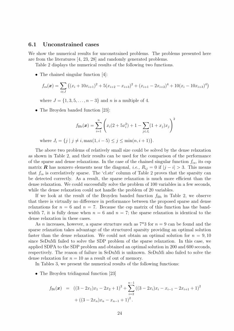
• The chained singular function [4]:

fcs(x) =∑i∈J

((xi + 10xi+1)

2 + 5(xi+2 − xi+3)2 + (xi+1 − 2xi+2)

4 + 10(xi − 10xi+3)4)

where J = {1, 3, 5, . . . , n− 3} and n is a multiple of 4.

• The Broyden banded function [23]:

fBb(x) =n∑

i=1

(xi(2 + 5x2

i ) + 1−∑j∈Ji

(1 + xj)xj

)2

where Ji = {j | j 6= i, max(1, i− 5) ≤ j ≤ min(n, i + 1)}.The above two problems of relatively small size could be solved by the dense relaxation

as shown in Table 2, and their results can be used for the comparison of the performanceof the sparse and dense relaxations. In the case of the chained singular function fcs, its cspmatrix R has nonzero elements near the diagonal, i.e., Rij = 0 if |j − i| > 3. This meansthat fcs is correlatively sparse. The ‘cl.str’ column of Table 2 proves that the sparsity canbe detected correctly. As a result, the sparse relaxation is much more efficient than thedense relaxation. We could successfully solve the problem of 100 variables in a few seconds,while the dense relaxation could not handle the problem of 20 variables.

If we look at the result of the Broyden banded function fBb in Table 2, we observethat there is virtually no difference in performance between the proposed sparse and denserelaxations for n = 6 and n = 7. Because the csp matrix of this function has the band-width 7, it is fully dense when n = 6 and n = 7; the sparse relaxation is identical to thedense relaxation in these cases.

As n increases, however, a sparse structure such as 7*3 for n = 9 can be found and thesparse relaxation takes advantage of the structured sparsity providing an optimal solutionfaster than the dense relaxation. We could not obtain an optimal solution for n = 9, 10since SeDuMi failed to solve the SDP problem of the sparse relaxation. In this case, weapplied SDPA to the SDP problem and obtained an optimal solution in 200 and 600 seconds,respectively. The reason of failure in SeDuMi is unknown. SeDuMi also failed to solve thedense relaxation for n = 10 as a result of out of memory.

In Tables 3, we present the numerical results of the following functions:

• The Broyden tridiagonal function [23]

fBt(x) = ((3− 2x1)x1 − 2x2 + 1)2 +n−1∑i=2

((3− 2xi)xi − xi−1 − 2xi+1 + 1)2

+ ((3− 2xn)xn − xn−1 + 1)2 .

24

chained singular Broyden bandedn cl.str εobj sparse dense n cl.str εobj sparse dense

12 3*10 1.1e-09 0.7 404.2 6 6*1 9.1e-10 20.5 20.416 3*14 9.0e-10 0.9 7523.1 7 7*1 2.4e-09 127.7 127.540 3*38 1.7e-09 2.1 — 8 7*2 4.2e-09 255.1 620.480 3*78 -2.9e-04 1.8 — 9 7*3 -1.0e+00 117.3. 3408.2

100 3*98 -3.6e-04 2.2 — 10 7*4 -1.0e+00 155.4 —

Table 2: Numerical results of the chained singular function and the Broyden banded function

• The chained wood function [4]:

fcw(x) = 1 +∑i∈J

(100(xi+1 − x2

i )2 + (1− xi)

2 + 90(xi+3 − x2i+2)

2 + (1− xi+2)2

+10(xi+1 + xi+3 − 2)2 + 0.1(xi+1 − xi+3)2),

where J = {1, 3, 5, . . . , n− 3} and n is a multiple of 4.

• The generalized Rosenbrock function [28]:

fgR(x) = 1 +n∑

i=2

{100

(xi − x2

i−1

)2+ (1− xi)

2}

.

Each of the above three functions has a band structure in its csp matrix, and therefore,the problems of large sizes can be handled efficiently. For example, the Broyden tridiagonalfunction fBt with 500 variables could be solved in 11.2 seconds with the accuracy of −6.3e-09. Without utilizing the correlative sparsity of the functions, it is not possible to obtainan optimal solutions of the smallest-sized problem in Table 3, as we experienced with thedense relaxation in the previous two problems. Note that the solutions are accurate in alltested cases.

Broyden tridiagonal chained wood generalized Rosenbrockn cl.str εobj sparse cl.str εobj sparse cl.str εobj sparse

100 3*98 -4.1e-9 2.4 2*99 -3.9e-7 0.4 2*99 2.6e-5 0.9200 3*198 -5.4e-6 4.7 2*199 -8.1e-7 0.7 2*199 1.6e-5 1.8300 3*298 -5.0e-9 6.6 2*299 -1.2e-6 1.1 2*299 3.0e-5 2.5400 3*398 -1.1e-8 11.0 2*399 -1.6e-6 1.4 2*399 1.2e-4 3.3500 3*498 -6.3e-9 10.2 2*499 -2.1e-6 1.7 2*499 +4.3e-5 4.5

Table 3: Numerical results of Broyden tridiagonal function, the chained wood function andthe generalized Rosenbrock function

Next, we present the numerical results of randomly generated problems. The aim of thetest using randomly generated problems is to observe the effects of increasing the numberof variables, the degree of the polynomials as well as the maximal size of cliques of the csp

25

graph of a POP. The dense relaxation could not handle the randomly generated problems ofthe sizes reported here, and we include only the numerical results from the sparse relaxation.

Let us describe how an unconstrained problem with artificial correlative sparsity is gen-erated randomly. We begin by constructing a chordal graph randomly such that the size ofevery maximal clique is not less than 2 and not greater than max.cl. From the chordal graph,we derive the set of maximal cliques {C1, . . . , C`} with 2 ≤ |Ci| ≤ max.cl (i = 1, . . . , `). Welet vCi

(x) = (xdk: k ∈ Ci) where 2d is the degree of the polynomial, and generate a positive

definite matrix V i ∈ S++(Ci) and a vector gi ∈ [−1, 1]#ACi2d−1 (i = 1, 2, . . . , `) randomly

such that the minimum eigenvalue σ of V 1, . . . , V ` satisfies the following relation:

σ ≥∑i=1

(‖gi‖2

√#ACi

2d−1

).

By using V i and gi, we define the objective function:

frand(x) =∑i=1

(vCi

(x)T V ivCi(x) + gT

i u(x,ACi2d−1)

).

It is easy to see that this unconstrained POP is guaranteed to have an optimal solution inthe compact set {x = (x1, . . . , xn) ∈ Rn | maxi=1,...,n |xi| ≤ 1}. A scaling with the maximumof the absolute values of the coefficients of frand(x) is used in numerical experiments.

The numerical results are shown in Tables 4, 5 and 6. Table 4 exhibits how the sparserelaxation performs for varying number of variables, Table 5 for raising the degree of theunconstrained problems, and Table 6 for increasing bounds of sizes of the cliques. For eachchoice of n, d and max.cl, we generated 50 problems. Each column of #solved indicates thenumber of the problems whose optimal solutions were obtained with εobj ≤ 10−5 out of 50problems.

n #clique max avr min #solved #notSol20 14.0 1.4 0.5 0.3 50/50 0/5040 28.7 3.1 1.3 0.7 50/50 0/5060 43.0 6.0 2.5 1.2 50/50 0/5080 57.1 30.4 6.1 2.0 50/50 0/50

100 71.7 19.1 6.5 2.7 50/50 0/50

Table 4: Randomly generated polynomials with max.cl= 4 and 2d = 4

2d #clique max avr min #solved #notSol4 21.3 2.0 0.9 0.5 50/50 0/506 21.0 168.4 15.2 1.9 50/50 0/508 21.4 1693.4 128.9 3.0 50/50 0/50

Table 5: Randomly generated polynomials with max.cl= 4, and n = 30

26

max.cl #clique max avr min #solved #notSol4 21.3 2.0 0.9 0.5 50/50 0/506 18.3 91.1 8.4 1.3 50/50 0/508 16.9 825.8 121.4 4.4 50/50 0/50

Table 6: Randomly generated polynomials with 2d = 4 and n = 30

In Table 4, we notice that the number of cliques increases with n. For problems oflarge numbers of variables and cliques such as n = 100 and #clique= 71.74, the sparserelaxation provides optimal solutions in most cases. The rate of success in obtaining anoptimal solution remains relatively unchanged for increasing n.

The numerical results in Table 5 displays the performance of the sparse relaxation forthe problem of n = 30 with degrees up to 8. The maximum size of cliques is fixed to 4. Asmentioned before, the size of the SDP relaxation of the POP of increasing degree becomeslarge rapidly even if the POP remains correlatively sparse. When d = 8, the average cputime is 128.9 and the maximum is 1693.4.

A large size of cliques used when a problem is generated also increases the complexityof the problem as shown in Table 6. We tested with the maximum size of cliques 4, 6, and8, and observe that cpu time to solve the corresponding problems grows very rapidly, e.g.121.4 average cpu seconds, 825.8 maximum cpu seconds for max.cl = 8. From the increaseof work measured by cpu time, we mention that the impact of the maximum size of cliquesis comparable to that of degree, and bigger than that of the number of variables.

6.2 Constrained cases

In this subsection, we deal with the following constrained POPs:

• Small-sized POPs from the literature [7, 11].

• Optimal control problems.

• Randomly generated maxcut problems.

• Randomly generated POPs.

Two of small-sized POPs, the problems 3.2 and 3.4, are from [7], and the rest of theproblems from [11]. The numerical results are presented in Tables 7 and 8. All the problemsare quadratic optimization problems (QOPs) except ’alkyl’ which involves polynomials ofdegree 3 in its equality constraints. In preliminary numerical experiment for some of thetest problems, we encountered severe numerical difficulties for badly-scaled problems and/orproblems with the complementarity condition. We incorporate all the tehcniques in Sec-tions 5.4, 5.5 and 5.6 into the dense and sparse relaxations for these problems. Specifically,we replaced each support AFk

ω−ωkfor the Lagange multiplier polynomial ϕk by the union

C of all cliques C` containing Fk as mentioned in Section 5.5, and added finite lower andupper bounds to all the variables of each problem so that the scaling technique and the valid

27

inequalities of the form 0 ≤ y� ≤ 1 given in Section 5.6 can work effectively. In addition,all the equality constraints were converted to two inequality constraints such that

f(x) = 0 =⇒ f(x) ≥ 0 and − f(x) + κ ≥ 0,

where κ = 10−5. Without these techniques, we could not solve many of the problems inTables 7 and 8.

The problems in Table 7 have known optimal values, hence, we compare the lowerbounds obtained by the sparse or dense relaxation to their optimal value in column εopt,which denotes

εopt =|the optimal value of SDP − the known optimal value of POP|

max{1, |the optimal value of POP|} .

In all cases, the sparse and dense relaxations attain reasonable accuracy with εopt ≤ 5.0e-2.ε′feas denotes the feasibility for the scaled problems at the approximate optimal solutionsobtained by the sparse and dense relaxations. We see that ε′feas is small in most of theproblems while the feasibility εfeas for the original problems at the approximate optimalsolutions becomes large. The lower bounds obtained by the sparse relaxation are as goodas the ones by the dense relaxations except the three problems ex5 2 2 cases1, 2 and 3. Inthese cases, the dense relaxation succeeds in computing accurate bounds while the sparserelaxation with order ω = 3 computes accurate bounds with the same quality.

The problems in Table 8 have no known optimal value or their best known optimal valuesare turned out to be inaccurate. The column SDPval denotes the lower bounds obtainedby the sparse or dense relaxations. In all cases, the attained accuracy εobj and feasibilityε′feas for the scaled problems are very small. Hence we can conclude that the column SDPvalprovides tight lower bounds for the optimal values of the test problems.

When we compare the performance of the sparse relaxation with the dense relaxationusing these problems in Tables 7 and 8, we observe that the sparse relaxation are muchfaster than the dense relaxation in large dimensional problems.

We should also mention that the technique given in Section 5.3 for reducing sizes ofrelaxations worked very effectively. For example, the sparse and dense relaxations of ex2 1 3without incorporating this tequnique tool 2.6 and 351.6 seconds, respectively, while 0.9 and13.6 seconds were consumed with this technique, respectively, as shown in Table 7.

We present numerical results from the discrete-time optimal control problems in [3]. Theproblem tested first (5 of [3]) is

minM−1∑i=1

(ny∑j=1

(yi,j +

1

4

)4

+nx∑j=1

(xi,j +

1

4

)4)

+

ny∑j=1

(yM,j +

1

4

)4

subject to yi+1 = Ayi + Bxi + (yTi Cxi)e (i = 1, . . . , M − 1), y1 = 0

yi ∈ Rny , (i = 1, . . . ,M), xi ∈ Rnx , (i = 1, . . . ,M − 1)

(38)

where A ∈ Rny×ny , B ∈ Rny×nx , and C ∈ Rny×nx are given by:

Ai,j =

0.5 if j = i,0.25 if j = i + 1,−0.25 if j = i− 1,

Bi,j =i− j

ny + nx

Ci,j = µi + j

ny + nx

,

28

spar

seden

sepro

ble

mn

ωε o

pt

ε obj

ε fea

sε′ fe

as

cpu

ε opt

ε obj

ε fea

sε′ fe

as

cpu

ex2

11

52

0.5e

-01

-1.9

e+00

0.0e

+00

0.0e

+00

0.2

0.5e

-01

-1.9

e+00

0.0e

+00

0.0e

+00

0.2

ex2

11

53

9.3e

-10

-3.0

e-06

0.0e

+00

0.0e

+00

1.8

6.6e

-06

-3.0

e-06

0.0e

+00

0.0e

+00

1.9

ex2

12

62

4.6e

-06

-3.3

e-11

-3.2

e-10

1.6e

-11

0.2

4.6e

-06

-4.4

e-11

0.0e

+00

0.0e

+00

0.3

ex2

13

132

1.3e

-06

-5.1

e-09

-3.5

e-09

-4.4

e-10

0.5

1.3e

-06

-1.6

e-09

-1.5

e-09

-1.8

e-10

7.7

ex2

14

62

2.2e

-06

-2.4

e-12

-4.7

e-11

-2.9

e-12

0.3

2.2e

-06

-2.4

e-12

-4.6

e-11

-2.9

e-12

0.3

ex2

15

102

3.7e

-09

-4.4

e-11

-5.4

e-10

-6.2

e-11

1.9

3.7e

-09

-4.4

e-11

-5.4

e-10

-6.2

e-11

1.8

ex3

11

82

0.7e

-01

0.0e

+00

-4.7

e+04

-5.8

e-02

0.6

0.7e

-01

0.0e

+00

-4.6

e+04

-5.8

e-02

2.6

ex3

11

83

6.3e

-09

0.0e

+00

-6.5

e-02

-2.2

e-08

5.5

2.2e

-07

0.0e

+00

-2.0

e-01

-6.9

e-08

597.

8ex

31

25

23.

0e-0

69.

9e-1

1-1

.4e-

07-4

.6e-

090.

73.

0e-0

69.

9e-1

1-1

.4e-

07-4

.6e-

090.

7ex

52

2ca

se1

92

0.1e

-01

0.0e

+00

-3.2

e+01

-1.3

e-04

1.8

1.6e

-05

0.0e

+00

-2.1

e-01

-8.4

e-07

3.4

ex5

22

case

19

36.

6e-0

40.

0e+

00-2

.3e-

01-9

.1e-

0729

5.9

——

——

—ex

52

2ca

se2

92

0.1e

-01

0.0e

+00

-7.2

e+01

-2.9

e-04

2.1

1.3e

-04

0.0e

+00

-2.7

e-01

-1.1

e-06

3.5

ex5

22

case

29

35.

8e-0

40.

0e+

00-8

.9e-

01-3

.6e-

0633

2.9

——

——

—ex

52

2ca

se3

92

0.3e

-01

0.0e

+00

-6.7

e+01

-2.7

e-04

1.9

1.6e

-05

0.0e

+00

-1.1

e-01

-4.4

e-07

2.6

ex5

22

case

39

32.

8e-0

40.

0e+

00-6

.0e+

00-2

.4e-

0533

6.5

——

——

—ex

53

222

20.

3e-0

10.

0e+

00-4

.1e+

00-1

.4e-

0253

.22.

7e-0

50.

0e+

00-1

.7e-

06-5

.7e-

0921

20.6

ex5

42

82

0.5e

+00

0.0e

+00

-4.3

e+05

-4.3

e-02

0.6

0.5e

+00

0.0e

+00

-4.3

e+05

-4.3

e-02

2.4

ex5

42

83

5.2e

-06

0.0e

+00

-3.2

e-01

-3.2

e-08

8.3

5.8e

-06

0.0e

+00

-8.1

e-01

-8.1

e-08

757.

4ex

91

113

26.

2e-0

60.

0e+

00-4

.5e-

06-1

.1e-

081.

56.

2e-0

60.

0e+

00-9

.2e-

07-2

.3e-

097.

7ex

91

210

25.

6e-0

60.

0e+

00-4

.1e-

06-1

.7e-

072.

85.

6e-0

60.

0e+

00-2

.6e-

07-1

.0e-

082.

1ex

91

513

22.

3e-0

40.

0e+

00-7

.2e-

05-2

.9e-

061.

02.

3e-0

40.

0e+

00-5

.0e-

05-2

.0e-

067.

6ex

91

814

27.

9e-0

60.

0e+

00-4

.1e-

01-4

.1e-

021.

37.

9e-0

60.

0e+

00-4

.1e-

01-4

.1e-

0220

.2ex

92

110

22.

2e-0

51.

3e-0

6-4

.9e-

05-3

.5e-

071.

22.

2e-0

56.

8e-0

8-3

.2e-

06-2

.1e-

082.

5ex

92

210

23.

0e-0

41.

0e-0

5-5

.2e+

00-1

.3e-

021.

62.

5e-0

48.

6e-0

6-3

.2e+

01-7

.9e-

026.

0ex

92

210

32.

1e-0

45.

3e-0

6-8

.0e-

01-2

.0e-

0336

.02.

9e-0

47.

6e-0

6-2

.5e+

01-6

.4e-

0215

92.4

ex9

25

82

2.3e

-06

6.2e

-07

-8.0

e-06

-8.0

e-08

0.6

2.5e

-06

7.2e

-08

-1.2

e-06

-1.2

e-08

0.9

ex9

26

162

2.0e

-04

1.2e

-05

-1.6

e+03

-4.1

e-02

0.9

2.0e

-04

-7.2

e-06

-3.8

e+03

-9.5

e-02

69.1

ex9

26

163

2.0e

-04

9.8e

-06

-9.3

e+02

-2.3

e-02

8.6

——

——

—ex

92

710

22.

3e-0

54.

7e-0

7-2

.0e-

05-1

.3e-

071.

32.

2e-0

52.

2e-0

9-4

.0e-

07-2

.7e-

092.

6ex

92

86

27.

7e-0

6-7

.9e-

07-4

.2e-

06-1

.0e-

080.

48.

2e-0

6-2

.5e-

07-3

.6e-

06-9

.0e-

090.

4

Tab

le7:

The

resu

lts

onso

me

pro

ble

ms

in[7

,11

]w

hos

eop

tim

alva

lue

isknow

n.

29

spar

seden

sepro

ble

mn

ωSD

Pva

lε o

bj

ε fea

sε′ fe

as

cpu

SD

Pva

lε o

bj

ε fea

sε′ fe

as

cpu

alkyl

142

-2.4

2e+

00-2

.0e-

03-2

.5e-

01-1

.1e-

026.

7-2

.41e

+00

-7.3

e-06

-3.2

e-02

-1.3

e-03

65.7

alkyl

143

-2.4

1e+

00-9

.0e-

09-3

.0e-

08-8

.3e-

1052

16.2

——

——

—ex

21

824

21.

56e+

04-1

.0e-

050.

0e+

000.

0e+

0030

4.6

1.56

e+04

-3.4

e-06

0.0e

+00

0.0e

+00

1946

.6ex

92

316

21.

85e+

010.

0e+

00-5

.7e-

06-9

.6e-

102.

31.

85e+

010.

0e+

00-7

.5e-

06-1

.2e-

0949

.7ex

92

48

23.

96e+

007.

5e-0

4-3

.1e-

02-7

.8e-

071.

53.

97e+

002.

7e-0

4-1

.6e-

02-4

.0e-

071.

8st

bpaf

1a10

2-4

.54e

+01

-5.5

e-08

-8.5

e-09

-4.7

e-11

1.4

-4.5

4e+

01-7

.6e-

09-2

.8e-

09-1

.5e-

111.

9st

bpaf

1b10

2-4

.30e

+01

-3.8

e-08

-2.8

e-08

-2.0

e-10

1.0

-4.3

0e+

01-4

.6e-

09-7

.2e-

10-1

.7e-

111.

7st

e05

52

7.05

e+03

0.0e

+00

-2.2

e+00

-1.9

e-09

0.3

7.05

e+03

0.0e

+00

-2.3

e-01

-2.0

e-10

0.4

ste0

710

2-1

.81e

+03

0.0e

+00

-8.1

e-05

-4.0

e-09

0.4

-1.8

1e+

030.

0e+

00-8

.8e-

06-4

.4e-

103.

0st

jcbpaf

210

2-7

.95e

+02

-1.1

e-07

0.0e

+00

0.0e

+00

2.1

-7.9

5e+

02-1

.1e-

070.

0e+

000.

0e+

002.

0

Tab

le8:

Num

eric

alre

sult

sfo

rsm

all-si

zed

pro

ble

ms

wit

hunknow

nop

tim

alva

lues

from

the

lite

ratu

res

[11]

.

30

respectively. Here, e denotes a vector of ones in Rny .The numerical results of the problem (38) are shown in Table 9, 10 and 11, which

display the results of the problem (38) with (nx, ny, µ) = (2, 4, 0), the problem (38) with(nx, ny, µ) = (2, 4, 0.5) and the problem (38) with (nx, ny, µ) = (1, 2, 1), respectively. Thevalues of nx, ny and M determine the size of the problem and µ is a parameter in Ci,j. Therelaxation order 2 was used for all cases. As we increase M from 6 to 30, the number ofvariables becomes bigger as indicated in the column of n. In all cases, the optimal solutionsare obtained with good accuracy.

Depending on the choice of µ, it results in different clique structures and the size ofthe resulting SDP varies. This size can affect greatly the performance of the relaxations.When we take µ = 0 in (38), the constraints are linear since C = O. Then, the cliques hassmaller number of elements than the ones from the constraints with nonlinear terms, whichenables the sparse relaxation to perform better in terms of cpu time. To see this, comparethe colum of cl.str of Table 9 with that of Table 10. For example, when M = 30 in Table9, it took 135.9 cpu seconds to have an optimal solution whereas 712.0 seconds in Table 10.Similarly, if we compare Table 10 and 11, we notice that the size of the cliques in Table 11is half the size in Table 10, while the cpu time of Table 11 is less than 1/100 times than thecpu time of Table 10. This shows how much efficiency can be improved using appropriateclique structures.

M n cl.str εobj εfeas cpu6 30 4*1+5*4+6*2+7*3+8*6 -2.5e-10 -6.9e-11 15.7

12 66 4*1+5*4+6*2+7*9+8*18 -9.0e-10 -8.2e-11 45.418 102 4*1+5*4+6*2+7*15+8*30 -5.0e-09 -2.1e-10 73.624 138 4*1+5*4+6*2+7*21+8*42 -1.0e-08 -2.8e-10 96.130 174 4*1+5*4+6*2+7*27+8*54 -7.9e-09 -1.2e-10 135.7

Table 9: Numerical results for the problem (38) with (nx, ny, µ) = (2, 4, 0). The relaxationorder ω = 2.

M n cl.str εobj εfeas cpu6 30 5*2+7*4+10*3 1.8e-09 -6.3e-10 76.7

12 66 5*2+7*4+10*9 2.9e-09 -7.7e-10 223.518 102 5*2+7*4+10*15 1.1e-09 -3.5e-10 369.424 138 5*2+7*4+10*21 3.2e-09 -1.0e-09 518.030 174 5*2+7*4+10*27 3.5e-09 -8.1e-10 663.7

Table 10: Numerical results for the problem (38) with (nx, ny, µ) = (2, 4, 0.5). The relaxationorder ω = 2.

The second problem (5 of [3]) is

min1

M

M−1∑i=1

(y2

i + x2i

)

subject to yi+1 = yi + 1M

(y2i − xi), (i = 1, . . . ,M − 1), y1 = 1.

(39)

31

Table 12 shows the results of (39) for various M . From the column cl.str, we notice that the

M n cl.str εobj εfeas cpu6 15 2*1+4*2+5*3 -1.3e-09 -3.9e-11 0.5

12 33 2*1+4*2+5*9 -1.8e-09 -3.0e-11 1.118 51 2*1+4*2+5*15 -6.9e-09 -7.2e-11 1.724 69 2*1+4*2+5*21 -1.0e-08 -1.1e-10 2.430 87 2*1+4*2+5*27 -1.2e-08 -9.9e-11 3.0

Table 11: Numerical results for the problem (38) with (nx, ny, µ) = (1, 2, 1). The relaxationorder ω = 2.

set of cliques has very few elements. The sparse relaxation can solve large-sized problemssince they have plenty of correlative sparsity. In fact, the sparse relaxation provides anoptimal solutions for the problems with almost 2000 variables, where the size of clique is 2or 3. It should be noted that the problem (39) is a QOP and that the relaxation order 1 wasused. In view of the discussion given in Section 5.4, the sparse relaxation is theoreticallyguaranteed to provide bounds with the same quality as the dense relaxation in all the casesof Table 12.

M n cl.str εobj εfeas cpu600 1198 2*1+3*598 3.4e-08 -2.2e-10 3.4700 1398 2*1+3*698 2.5e-08 -8.1e-10 3.3800 1598 2*1+3*798 5.9e-08 -1.6e-10 3.8900 1798 2*1+3*898 1.4e-07 -6.8e-10 4.5

1000 1998 2*1+3*998 6.3e-08 -2.7e-10 5.0

Table 12: Numerical results from problem (39). The relaxation order ω = 1.

We now consider the maxcut problem. Suppose that an undirected graph G = (V, E) isgiven, where V = {1, . . . , n} is the set of nodes and E is the set of edges, respectively. Fora subset S ⊆ V , a set of edges {{i, j} ∈ E|i ∈ S, j 6∈ S} is called a cut. Then the maxcutproblem is to find a cut that has the maximum number of edges. We formulate the maxcutproblem as an equality constrained POP:

maximize∑

{i,j}∈E

(1− xixj)/2

subject to x2i = 1 (i ∈ V ).

(40)

See [10] or [27] for details of this formulation.In [25] and [26], it is shown that a further reduction of the variables is possible in the

SOS relaxation if we deal with the integer equality constraints directly. However, we do notuse this technique because the purpose of this experiment is to estimate the effect of usingcorrelative sparsity of POPs. To incorporate techniques only useful for integer programmingis not the subject of this paper.

32

The csp matrix of (40) has the same sparsity pattern as the adjacency matrix of G withthe diagonal. Therefore, the sparse relaxation can be applied efficiently when the chordalextension of the graph is sparse. To obtain such a sparse graph, we generate edges in a bandof the matrix. Specifically, we use two parameters, band-width b and rate r to generate arandom graph. We first connect nodes i and i + 1 (i = 1, 2, . . . , n − 1), and then nodes iand j such that 1 < |i− j| ≤ b with probability r. In this experiment, we choose b = 7, andr = 0.3333. Each node has about six edges on average with this parameter selection.

Notice that in Tables 13 and 14, n, the number of variables of POP, is equal to the size ofnodes. For each size of nodes, we performed 10 trials. A problem is considered to be solvedwhen εobj < 10−3 and εfeas < 10−3. The relaxation order is fixed to 2, which was decided bysome preliminary experiments on what value of relaxation order should be used to obtainsolutions. Most of the small-sized problems in Table 13 could be solved to the optimumwith the relaxation order 2 and none of the problems was solved with the relaxation order 1.

We observe in Table 13 that the cpu time is significantly reduced for the sparse relaxationcompared with the dense relaxation. In all problems, the optimal values of the dense andsparse relaxations coincide up to 9 digits, although theoretically this is not ensured for thesparse relaxation with the relaxation order 2.

We can also see that the sparse relaxation is less influenced by the size of the graph,while in the dense relaxation, the difference in the size of nodes by just one is critical to thecpu time.

sparse densen #clique max ave min max ave min #solved #notSol

10 5.9 1.3 0.7 0.3 32.9 28.4 20.8 10/10 0/1011 6.5 2.8 1.1 0.4 136.7 84.3 50.8 9/10 1/1012 7.4 2.0 1.1 0.3 305.4 181.8 127.4 10/10 0/1013 7.8 4.6 1.8 0.8 863.7 443.3 257.6 9/10 1/1014 8.9 3.0 1.8 0.8 1627.7 1003.7 540.9 9/10 1/1015 9.6 4.0 2.3 0.9 2456.3 1975.4 1274.0 10/10 0/10

Table 13: Numerical results from the maxcut problem. The relaxation order ω = 2.

Table 14 shows the results of the sparse relaxation with larger size of nodes. The problemwith 120 nodes can be solved in less than 300 seconds on average. The average cpu timeincreases by O(n1.6) approximately. However, the accuracy of the solution deteriorates asthe size of nodes increases.

n #clique max avr min #solved #notSol60 47.2 15.9 41.5 15.9 7/10 3/1080 64.0 136.3 71.6 29.6 2/10 8/10

100 79.5 213.2 96.1 49.2 1/10 9/10120 95.3 218.0 134.4 75.8 1/10 9/10

Table 14: Sparse relaxation with increasing number of nodes in the maxcut problem. Therelaxation order ω = 2.

33

Finally, we present the numerical results from randomly generated constrained problems:

min∑j=1

fTj u(x,ACj

2d )

subject to vCj(x)T V jvCj

(x) + gTj u(x,ACj

2d−1) ≤ 0 (j = 1, . . . , `),

(41)

where the set {C1, . . . , C`} is a set of maximal cliques generated in the same way as randomlygenerated unconstrained test problems, vCj

(x) = (xdk: k ∈ Cj), f j are randomly generated in

[−1, 1]#ACj2d , and positive definite matrices V j ∈ S++(Cj) and gj (j = 1, . . . , `) are randomly

generated such that the minimum eigenvalue of V j is greater than ‖gj‖ ×√

#ACj

2d−1.

The value of the relaxation order needs to be chosen prior to solving a problem. However,its proper value is not known in many problems. As mentioned in Secion 5.2, raising therelaxation order gradually provides more accurate solutions, but it takes increasingly longerto solve. In this experiment, the problem is solved with an initial relaxation order, and if itis successful to get a solution within required accuracy, it is regarded as solved. Otherwise,the relaxation order is raised by 1 and the problem is tried again. We generated 10 problemsfor each choice of n. In every experiment, the tolerance for both εobj and εfeas is set to 10−5,and the initial relaxation order 2. For the problems that could not be solved, we increasethe relaxation order by 1, and apply the sparse relaxation again. As shown in Table 17,for n = 10, 7 out of 10 problems were tried again with increased relaxation order 3. It isimportant to solve the problem with low relaxation order because increasing the relaxationorder by 1 needs a great deal of additional cpu time. This repetitive strategy is appropriatewhen proper relaxation order is not known in advance.

n ω #clique max avr min #solved #notSol10 2 6.4 0.5 0.3 0.2 4/10 6/10

3 1.1 0.7 0.3 6/6 0/620 2 14.0 1.1 0.7 0.5 0/10 10/10

3 4.7 3.0 1.8 9/10 1/104 37.3 37.3 37.3 0/1 1/1

30 2 21.6 1.7 1.0 0.6 0/10 10/103 30.1 8.7 2.6 8/10 2/104 67.7 58.1 48.5 0/2 2/2

40 2 28.7 2.1 1.5 0.9 0/10 10/103 43.6 17.2 4.1 9/10 1/104 595.8 595.8 595.8 1/1 0/1

50 2 36.5 3.5 2.0 1.4 0/10 10/103 151.1 40.5 8.0 7/10 3/104 4320.2 3101.3 677.3 1/3 2/3

Table 15: Problem (41) with max.cl = 4 and 2d = 4

It is shown in Tables 15, 16, and 17 that approximately 80 % of the problems were solvedby raising the relaxation order except the case n = 50 in Table 15. There remained someproblems that could not be solved by the sparse relaxation. The main reason of the failure

34

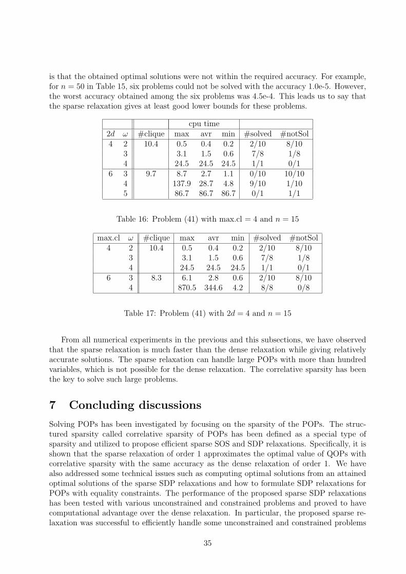
is that the obtained optimal solutions were not within the required accuracy. For example,for n = 50 in Table 15, six problems could not be solved with the accuracy 1.0e-5. However,the worst accuracy obtained among the six problems was 4.5e-4. This leads us to say thatthe sparse relaxation gives at least good lower bounds for these problems.

cpu time2d ω #clique max avr min #solved #notSol4 2 10.4 0.5 0.4 0.2 2/10 8/10

3 3.1 1.5 0.6 7/8 1/84 24.5 24.5 24.5 1/1 0/1

6 3 9.7 8.7 2.7 1.1 0/10 10/104 137.9 28.7 4.8 9/10 1/105 86.7 86.7 86.7 0/1 1/1

Table 16: Problem (41) with max.cl = 4 and n = 15

max.cl ω #clique max avr min #solved #notSol4 2 10.4 0.5 0.4 0.2 2/10 8/10

3 3.1 1.5 0.6 7/8 1/84 24.5 24.5 24.5 1/1 0/1

6 3 8.3 6.1 2.8 0.6 2/10 8/104 870.5 344.6 4.2 8/8 0/8

Table 17: Problem (41) with 2d = 4 and n = 15

From all numerical experiments in the previous and this subsections, we have observedthat the sparse relaxation is much faster than the dense relaxation while giving relativelyaccurate solutions. The sparse relaxation can handle large POPs with more than hundredvariables, which is not possible for the dense relaxation. The correlative sparsity has beenthe key to solve such large problems.

7 Concluding discussions

Solving POPs has been investigated by focusing on the sparsity of the POPs. The struc-tured sparsity called correlative sparsity of POPs has been defined as a special type ofsparsity and utilized to propose efficient sparse SOS and SDP relaxations. Specifically, it isshown that the sparse relaxation of order 1 approximates the optimal value of QOPs withcorrelative sparsity with the same accuracy as the dense relaxation of order 1. We havealso addressed some technical issues such as computing optimal solutions from an attainedoptimal solutions of the sparse SDP relaxations and how to formulate SDP relaxations forPOPs with equality constraints. The performance of the proposed sparse SDP relaxationshas been tested with various unconstrained and constrained problems and proved to havecomputational advantage over the dense relaxation. In particular, the proposed sparse re-laxation was successful to efficiently handle some unconstrained and constrained problems

35

that were impossible to obtain optimal solutions with the dense relaxation, e.g. the gener-alized Rosenblock function with dimension n = 500 and a QOP with dimension n = 1998arising from discrete optimal control. This demonstrates the efficiency and effectiveness ofthe proposed sparse relaxation for POPs with correlative sparsity.

The proposed sparse relaxation for a correlative sparse POP leads to an SDP that canmaintain the sparsity for primal-dual interior-point methods. This is based on the factthat if a POP to be solved is correlatively sparse, the resulting SDP relaxation inheritsthe structured sparsity. In each iteration of a primal-dual interior-point method for solvingan SDP, a square system of linear equations, which is often called the Schur complementequation, is solved to compute a search direction. The coefficient matrix of this systemis positive definite and fully dense in general even when all data matrices of an SDP tobe solved are sparse. However, the sparse SDP relaxation of a correlatively sparse POPpossesses sparsity in the coefficient matrix. This is an important advantage of the proposedsparse relaxation. Indeed, the coefficient matrix of the Schur complement equation in mostof SDPs solved in Section 6 is sparse. Among software packages implementing primal-dual interior-point methods, SeDuMi [34] handles SDPs with this sparsity in the coefficientmatrix of the Schur complement equation and provides solutions with efficiency while thecurrent version of SDPA [35] developed by the authors’ group is not equipped with the sparseCholesky factorization for the Schur complement equation, showing slow performance forPOPs with the correlative sparsity. This is the main reason that SeDuMi has been a choiceof the numerical experiments instead of SDPA.

We encountered severe numerical difficulties during preliminary numerical experiments.The techniques presented in Section 5 were very effective to overcome the difficulties andto enhance the performance of the sparse and dense relaxations. Besides the problemspresented in Tables 7 and 8, the sparse and dense relaxations could successfully solve small-sized problems ex2 1 1, ex2 1 2, ex2 1 4, ex3 1 2, ex3 1 4, ex9 2 3 and ex9 2 5 from [11].The three problems ex9 1 4, haverly and house from [11], however, could not be solvedbecause of numerical troubles resulted from SeDuMi. The failure has to be investigatedmore rigorously, but some SDPs generated as relaxations of POPs may be very difficultto solve. Additional techniques to resolve this difficulty are to be developed. The size ofthe SDP relaxation of a POP continue to play an an important role to obtain a solutionsuccessfully, although applying the sparse relaxation reduces the size of the resulting SDPsignificantly compared with that of the dense relaxation. As mentioned, increasing thedimension n and/or the degree d of polynomials in a POP makes the size of the resultingSDP larger. Furthermore, even when n and d are small, the relaxation order and/or thesize of the maximum cliques can increase the size of the SDP significantly. Reducing thesize of the SDP further is a key remaining issue to solve more challenging POPs.

References

[1] C. Ashcraft, D. Pierce, D. K. Wah and J. Wu, “The reference manual for SPOOLES,release 2.3: An object oriented software library for solving linear systems of equations,”Boeing Shared Services Group, Seattle, WA, January 1999.

[2] J. R. S. Blair and B. Peyton, “An introduction to chordal graphs and clieque trees,”In: A. George, J. R. Gilbert and J. W. H. Liu des, Graph Theory and Sparse Matrix

36

Computation, Springer, New York, pp.1-29, 1993.

[3] T. F. Coleman and A. Liao, “An efficient trust region method for unconstraineddiscrete-time optimal control problems”, Comp.Opt.Appl., 4 (1995) 47–66

[4] A. R. Conn, N. I. M. Gould and P. L. Toint, “Testing a class of methods for solvingminimization problems with simple bounds on the variables”, Math.Comp., 50 (1988)399–430

[5] M. D. Choi, T. Y. Lam, and B. Reznick, “Sums of squares of real polynomials”,Proceedings of Symposia in Pure Mathematics, 58 (1995) 103-126.

[6] G.Ewald, D.G.Larman and C.A.Rogers, “The directions of the line segments and of ther-dimensional balls on the boundary of a convex body in Euclidean space”, Mathematica17 (1970) 1-20.

[7] C. Floudas, P.Pardalos, C. Adjiman, W. Esposito, Z. Gumus, S. Harding, J. Klepeis,C. Meyer and C. Schweiger Handbook of test problems in local and global optimizationKluwer Academic Publishers, 1999

[8] T. Fujie and M. Kojima, “Semidefinite programming relaxation for nonconvexquadratic programming”, Journal of Global Optimization, 10 (1997) 367-380.

[9] M. Fukuda, M. Kojima, K. Murota and K. Nakata, “Exploiting sparsity in semidef-inite programming via matrix completion I: General framework,” SIAM Journal onOptimization, 11 (2000) 647-674.

[10] M. X. Goemans and D. P. Williamson, “Improved approximation algorithms for max-imum cut and satisfiability problems using semidefinite programming”, Journal ofAssoc. Compute. Mach., 42 (1995) 1115-1145.

[11] GLOBAL Library, http://www.gamsworld.org/global/globallib.htm

[12] D. Henrion and J. B. Lasserre, “GloptiPoly: Global optimization over polynomialswith Matlab and SeDuMi”, ACM Trans. Math. Soft., 42 (2),(2003) 165-194.

[13] D. Henrion and J. B. Lasserre, “Detecting global optimality and extracting solutions inGloptiPoly”, LAAS-CNRS Research Report No. 93541, October 2003. (To appear as acontributed chapter in the book D. Henrion, A. Garulli(Editors). Positive polynomialsin control. Lecture Notes on Control and Information Sciences, Springer Verlag, toappear in 2005.)

[14] D. Henrion and J. B. Lasserre, “A convergence hierarchy of LMI relaxations for poly-nomial matrix inequalities”, Laboratoire d’Analyse et d’Architecture des Syst‘emes,Centre National de la Recherche Scientifique, 7 Avenue du Colonel Roche, 31 077Toulouse, cedex 4, France, August 2004.

[15] D. Hilbert, “Uber die Darstellung definiter Formen als Summe von Formenquadraten”,em Math. Ann., 32 (1888) 342-350; see Ges. Abh., 2 (1933) 154-161, Springer, Berlin,reprinted by Chelsea, New York, 1981.

37

[16] C.W. J. Hol and C.W. Scherer, Sum of squares relaxations for polynomial semidefiniteprogramming, Proc. Symp. onMathematical Theory of Networks and Systems (MTNS),Leuven, Belgium, 2004.

[17] G. Karypis and V. Kumar, “METIS — A software package for partitioning unstruc-tured graphs, partitioning meshes, and computing fill-reducing ordering of sparse ma-trices, version 4.0 —,” Department of Computer Science/Army HPC Research Center,University of Minnesota, Minneapolis, MN, September, 1998.

[18] S. Kim, M. Kojima and H. Waki, “Generalized Lagrangian duals and sums of squaresrelaxations of sparse polynomial optimization problems”, Research Report B-395,Dept. of Mathematical and computing Sciences, Tokyo Institute of Technology, Me-guro, Tokyo 152-8552, September 2003. Revised July 2004. To appear in SIAM Journalon Optimization.

[19] M. Kojima, “Sums of squares relaxations of polynomial semidefinite programs,” Re-search Report B-397, Dept. of Mathematical and computing Sciences, Tokyo Instituteof Technology, Meguro, Tokyo 152-8552, November 2003.

[20] M. Kojima, S. Kim and H. Waki, “A general framework for convex relaxation ofpolynomial optimization problems over cones”, Journal of Operations Research Societyof Japan, 46 2 (2003) 125-144.

[21] M. Kojima, S. Kim and H. Waki, “Sparsity in sums of squares of polynomials”, Re-search Report B-391, Dept. of Mathematical and computing Sciences, Tokyo Instituteof Technology, Meguro, Tokyo 152-8552, June 2003. Revised June 2004. To appear inMathematical Programming.

[22] M. Kojima and M. Muramatsu, “An extension of sums of squares relaxations to poly-nomial optimization problems over symmetric cones,” Research Report B-406, Dept. ofMathematical and computing Sciences, Tokyo Institute of Technology, Meguro, Tokyo152-8552, April 2004.

[23] J. J. More, B. S. Garbow and K. E. Hillstrom, “Testing Unconstrained OptimizationSoftware”, ACM Trans. Math. Soft., 7, (1981) 17–41

[24] J. B. Lasserre, “Global optimization with polynomials and the problems of moments”,SIAM Journal on Optimization, 11 (2001) 796–817.

[25] J. B. Lasserre, “An explicit equivalent positive semidefinite program for nonlinear 0-1programs”, SIAM Journal on Optimization, 12 (2002) 756–769.

[26] M. Laurent, “A comparison of the Sherali-Adams, Lovasz-Schrijver, and Lasserre relax-ations for 0-1 programming”, Mathematics of Operations Research, 28 (2003) 470–496.

[27] M. Muramatsu and T. Suzuki, “A New Second-Order Cone Programming Relaxationfor MAX-CUT Problems”, Journal of Operations Research of Japan ,46 (2003) 164–177.

38

[28] S. G. Nash, “Newton-Type Minimization via the Lanczos method”, SIAM J.Numer.Anal.,21 (1984) 770–788.

[29] P. A. Parrilo, “Semidefinite programming relaxations for semialgebraic problems”,Mathematical Programming, 96 (2003) 293-320.

[30] S. Prajna, A. Papachristodoulou and P. A. Parrilo, “SOSTOOLS: Sum of SquaresOptimization Toolbox for MATLAB – User’s Guide”, Control and Dynamical Systems,California Institute of Technology, Pasadena, CA 91125 USA, 2002.

[31] M. Putinar, “Positive polynomials on compact semi-algebraic sets”, Indiana UniversityMathematics Journal, 42 (1993) 969–984.

[32] B. Reznick, “Extremal psd forms with few terms”, Duke Mathematical Journal, 45(1978) 363-374.

[33] M. Schweighofer, “Optimizationof polynomials on compact semialgebraic sets”, Work-ing paper, Universitat Konstanz, Fachbereich Mathematik und Statstik, 78457 Kon-stanz, Allemagne, Germany, April 2004.

[34] J. F. Strum, “SeDuMi 1.02, a MATLAB toolbox for optimizatin over symmetric cones”,Optimization Methods and Software, 11 & 12 (1999) 625-653.

[35] M. Yamashita, K. Fujisawa and M. Kojima, “Implementation and evaluation of SDPA6.0 (SemiDefinite Programming Algorithm 6.0)”, Optimization Methods and Software,18 (2003) 491-505.

39