Estimating Arrival Rate of Nonhomogeneous Poisson Processes

with Semidefinite Programming

Farid Alizadeh ∗†

October 15, 2011

Abstract

We present a method of estimating arrival rate of nonhomogeneous Poisson processes from afinite set of observed data. Both one-dimensional time dependent, and multi-dimensional timeand location dependent rates are considered. The arrival rate is a nonnegative function of time(or time and location). We assume that it is a smooth function with continuous derivativesof up to certain order k. We estimate the rate function by one or multi-dimensional splines,with the additional condition that the underlying rate function is nonnegative. This approachresults in optimization over nonnegative polynomials which can be modeled with semidefiniteprogramming. We also describe a method which requires only linear constraints. Numericalresults based on e-mail arrival and highway accidents are presented.

1 Introduction

In this article we present a method of estimating the arrival rate of nonhomogeneous Poissonprocesses based on observed arrival data. Our approach is based on maximum likelihood estimation,and the key constraint is that the arrival rate function λ(·) is a nonnegative function throughout.We also assume that this function is continuous and smooth (that is differentiable of order k forsome integer k).

Here we present a summary of two papers which use optimization over the cone of nonnegativefunctions by approximating it from within using nonnegative splines. The first paper [AENR08] isexclusively concerned with one-dimensional Poisson processes, that is λ(t) is a function time only.The second [PA11a] deals with–in principle–multi-dimensional Poisson processes, that is λ(t) is afunction of several variables included in the vector t. These variables can be time and location,and may include one two or more coordinates to specify the spatial information. In [PA11a] only aone dimensional spatial information is used. Therefore, the rate function is λ(t, s) with t the timeand s the one dimensional space information.

In [AENR08] the motivational problem was estimating arrival of e-mails, queries to databases,and hits on web sites. Although in such cases the independence assumption at a local level can beviolated (for instance bursts of e-mail arrivals may be sent as a result of “flame wars”, or peoplemay encourage each other to go to certain web sites), the assumption was that these infractionsare relatively minor. However the variability of rates in all cases were significant.

Another key property in these cases was periodicity. For instance the pattern of e-mail arrivalswas more frequent during working hours, and became less frequent on weekends and at nights. So

∗Management Science and Information Systems Department, Rutgers–State University of New Jersey, Piscataway,

NJ, 08854, USA. E-mail:alizadeh@rutcor.rutgers.edu†Research supported in part by National Science Foundation Grant number CMMI-0935305.

1

an a priori assumption of one-week period was reasonable. The main computational experiment in[AENR08] was a set of 10,000 e-mails arrived over a period of sixty weeks1.

In the multi-dimensional case the nonnegativity constraint is not easily modeled by semidefiniteprogramming. However the sum-of-squares property is. So the approach taken in [PA11a] isto estimate nonnegative, multivariate functions, by multivariate biquadratic polynomials splines,where over each patch, the corresponding polynomial is assumed to be a sum-of-squares polynomial.This approach also results in semidefinite constraints.

In the remainder of this article we explain results of [AENR08] and [PA11a] in a unified frame-work, and suggest that the approach taken may be useful in other statistical learning contexts.

2 Nonhomogeneous Poisson Likelihood functions and problem mod-

els

We assume that a sequences of observations x1,x2, . . . ,xN ∈ ∆ ⊆ Rd are generated by a multi-

dimensional nonhomogeneous process with arrival rate λ : ∆→ R+. The set ∆ = [0, T1]× [0, T2]×· · · × [0, Td]. We assume that λ is a continuous and smooth of at least order k. It is also possiblethat λ is periodic with respect to some of its coordinates.

In most realistic situations, the observed data are noisy. For instance, if in some componentxi indicates time, it may be that the observations have been rounded to the nearest minute orhour. And if it is distance, it may have been rounded to the nearest meter, or mile. Therefore,it is reasonable to partition the range of each of arrivals into regions ∆i, for i ∈ I and I issome index set. Then, our data will be the number ni of arrivals in each ∆i. In this case thedistribution of the number of items in each d-dimensional set ∆i will follow nonhomogeneousPoisson distribution. Thus, the likelihood function associated with observed arrivals ni gatheredin the vector n = (n1, . . . , nN ), conditioned on the rate function λ(·), is given by:

Ln(λ) = Pr(number of arrivals = N |λ) · Pr(distribution of exactly N arrivals = n |λ)

=IN

N !e−I ·

N !∏

i∈I ni!

∏

i∈I

(∫

∆iλ

I

)ni

=e−I

∏

i∈I ni!

∏

i∈I

(∫

∆i

λ

)ni

, where I =

∫

∆λ.

The optimization problem is to maximize this likelihood function over a suitable space of for λ,and subject to λ nonnegative. Additional conditions for periodicity can be also be included in thisoptimization model.

We first observe that maximizing Ln is equivalent to maximizing its logarithm (after removingconstant terms):

f(λ)def= ln

((

∏

i∈I

ni!

)

Ln(λ)

)

= −

∫

∆λ +

∑

i∈I

ni ln

∫

∆i

λ. (1)

Since under certain conditions this function is concave, we will use it as our objective function.However, further simplifications are possible.

It can be shown that if there is feasible function λ0 with a strictly positive integral∫

∆ λ0 > 0,then, at any optimal solution λ∗,

∫

∆ λ = N , see [PA11a, Lemma 1]. In other words, the expected

1This data was collected around 2003 when the onslaught of Spam, especially from around the world, had not yet

grown. Thus, the number of e-mails received were indeed much less on, say, Friday afternoons. Our approach should

still work today, and the rate functions should still exhibit a weekly periodic rate, albeit with somewhat different

pattern of frequency

2

number of arrivals with respect to any maximum likelihood solution arrival rate equals the numberof observed arrivals, N . Thus, we can remove the quantity

∫

∆ λ, and add the linear equalityconstraint

∫

∆ λ = N to the model.

2.1 Nonparametric approach to estimating λ in one variable

In the optimization problem the likelihood function 1 is to be maximized, and the “decision variable”λ is actually a function, which we require it to be continuous and smooth of some given total order,say k. To make this problem well-posed we may require that it belong to a closed linear functionspace (such as, for instance a Hilbert-Sobolev space with appropriate parameters.)

Since Hilbert-Sobolev spaces are infinite dimensional we must approximate λ by searching ap-propriate finite dimensional function spaces. In General, if the (infinite dimensional) linear func-tional space is Ω, to approximate it, we select a nested sequence of finite dimensional spacesΩ0 ⊂ Ω1 ⊂ · · · ⊂ Ω. Furthermore, for each pair of integers i < j, Ωi must be a subspace of Ωj , andall are subspaces of Ω. Finally, we require that

⋃

i Ωi be dense in Ω.The strategy of nonparametric estimation of λ(·) ∈ Ω can now be summarized as follows. For an

integer k find the most likely λk(·) ∈ Ωk, subject to λk(·) ≥ 0, and other required conditions (suchas periodicity, etc.). In this case we have a convex optimization problem, which sometimes (butnot always!) is computationally tractable. Then one should increase k and solve the correspondingoptimization problem. One must balance between accuracy, and overfitting. Strategies such ascross validation or AIC or BIC criteria may be used to guard against overfitting.

We use polynomial splines, but our framework is general enough to work with many other linearfunctions spaces. In the following sections we outline in greater detail the case of univariate andbivariate λ, approximated by polynomial splines.

2.2 The significance of periodicity

Like any statistical estimation problem, we should expect that the more data is available, the moreaccurate our estimates should be. However, in the arrival estimation problem this simple principleis not necessarily true. Let us first consider the one-dimensional case.

Suppose λ(t) is the sought after arrival rate, and t is time. Here, it is not clear what exactlythe meaning of “more data” is. Since we have no control over the arrivals, it may appear that theonly way to gather more data is to make observations over a longer period of time. However, in theneighborhood of each time stamp ti, the function λ(·), in general, is unique: further observationsat other time stamps tj will not give any new information on the behavior of λ(·) at ti. In effect,we have only one observation for some values of t and none for the rest.

This problem can be solved if λ(·) is periodic. If the period of the function is, say T , thenobservation in the interval [kT, (k + 1)T ] are essentially new observations of the period [0, T ]. Inthis way, by making observations in longer period of time, we can gather more data, and hope tohave more accurate estimates.

For multi-dimensional Poisson processes, the situation is similar. Here, we need λ(·) to beperiodic with respect to at least one of the variables. Then by making more observations alongthat variable we can get more data and improve our estimates. For instance, consider the arrival ofaccidents in a certain stretch of a highway, observed both at mileage marks from one end, and attime stamps during the day. Assuming that occurrence of accidents follows traffic patterns, whichin turn are periodically dependent on a work day schedule, we will have an arrival rate λ(t, s),where t is time and s is mileage point. Thus, in this setup, λ is periodic with respect to t with

3

a period of one day. By observing and recording traffic accidents over many days, we can gathermore data and thus hope to estimate λ more accurately.

It is possible to generalize the problem to the case where the length of the period for one (ormore) variables are unknown. Also, one may have other, more complicated patterns of repetitionin λ, such as periodicity multiplied by an upward or downward trend. In this article we restrictourselves to the case where periodicity is simple and known a priori.

3 Nonnegative polynomial splines and semidefinite programming

I: The univariate case

In this section we consider a one-dimensional problem, that is arrivals are a sequence of time stamps0, t1, t2, · · · in the time span [0, T ]. The observations themselves may be noisy, so as indicated earlier,we subdivide the range [1, T ] into 0, q1, . . . , qν , intervals, and record the number nj of arrivals inthe interval [qj−1, qj ]. In this case, the data is the vector n = (n1, . . . , nν) and the log-likelihoodfunction is

Ld(n,q, λ) =

ν∑

j=1

(

nj ln

(

∫ qj

qj−1

λ(t) dt

)

− ln nj!

)

−

∫ qν

q0

λ(t) dt. (2)

The optimization problem now ismaxλ≥0

Ld(n,q,λ)

Since the term∑

j ln nj! a constant, it can be removed.Now, λ is a continuous function, with continuous derivatives of order up to k. Suppose [0, T ]

is divided into m intervals 0 = a0 < a1 < · · · < am = T . Then a polynomial spline of order kis a function λk(t), such that on each interval [aj, aj+1] it equals a polynomial pj(t) of degree k.Furthermore, at the knot points aj , λ(·) must be continuous, and with continuous derivatives oforders up to k. With this model, the decision variables are the m(k +1) coefficients of polynomials

pj(t). To impose continuity and smoothness, the linear equality constraints p(r)j−1(aj) = p

(r)j (aj)

must be added to constraints for each of pj , and each r = 0, . . . , k − 1 and each j = 1, . . . ,m.The key constraint here is that λ(t) ≥ 0 for t ∈ [0, T ], which translates into pj(t) ≥ 0 for

all t ∈ [aj−1, aj], for j = 0, . . . ,m − 1. It turns out, in general, that the condition p(t) ≥ 0 fort ∈ [a, b] is SD-representable, see [BTN01],[NN94] for definition of SD-representable. This meansthat requiring a polynomial to be nonnegative over an interval can be characterized by positivesemidefiniteness of some matrices. Specifically, let h ≥ 0, and Eh

ℓ be the (h + 1) × (h + 1) matrixgiven by

(

Ehℓ

)

ij=

1, i + j = ℓ0, i + j 6= ℓ,

0 ≤ i, j ≤ h.

define the inner product of matrices by

X • Ydef=∑

ij

XijYij .

Then it can be shown that p0 + p1t + · · · + pktk ≥ 0 for all t ∈ [a, b], if and only if there there are

positive semidefinite matrices X and Y such that

4

When k is odd:

p0 = −aEh0 •X + bEh

0 • Y (3)

p1 = (Eh0 − aEh

1 ) •X + (bEh1 − Eh

0 ) • Y

p2 = (Eh1 − aEh

2 ) •X + (bEh2 − Eh

1 ) • Y

...

pℓ = (Ehℓ−1 − aEh

ℓ ) •X + (bEhℓ − Eh

ℓ−1) • Y

...

pk = Ehk−1 •X − Eh

k • Y.

When k is even: In this case set h = k/2 and

p0 = Eh0 •X − abEh−1

0 • Y

p1 = Eh1 •X +

(

(a + b)Eh−10 − abEh−1

1

)

• Y

p2 = Eh2 •X +

(

−Eh−10 + (a + b)Eh−1

1 − abEh−12

)

• Y

...

pℓ = Ehℓ •X +

(

−Eh−1ℓ−2 + (a + b)Eh−1

ℓ−1 − abEh−1ℓ

)

• Y

...

pk = Ehk •X − Eh−1

k−2 • Y

In both cases the set of constraints are semidefinite constraints. We should mention that in themost popular case when cubic splines are used, h = 2, and matrices X and Y are actually 2 × 2.It is well-known that in this special case the cone of positive semidefinite symmetric matrices areactually the three dimensional Lorentz or second order cone, see [AG03].

Now, the condition that a polynomial spline of degree at most k, and over the knot set 0 =a0 < a1 < . . . < aN = T , be nonnegative is expressed by requiring

1. each pj(t) ≥ 0 for all t ∈ [aj−1, aj ],

2. at each knot point aj, we must have p(r)j−1(aj) = p

(r)j−1(aj) for each r = 0, 1, . . . , k − 1,

3. and if the spline is periodic, then also p(r)N (aN ) = p

(r)1 (a0), for r = 0, 1, . . . , k − 1.

The resulting constraint set is a structured semidefinite program with many SDP constraints ofsmall order, since in spline approximations, the degree k is typically small.

The objective function, defined as the log-likelihood function, is not linear, but it is concave inthe decision variables pij. Thus, we have a tractable convex optimization problem which can besolved using existing open-source or commercial software.

4 Nonnegative polynomial splines and semidefinite programming

II: The multivariate case

When the nonhomogeneous Poisson process is multi-dimensional there are some similarities to one-dimensional case, but there are also significant differences. We have already noted the issue of

5

periodicity for at least one variable. We now sketch difficulties, mostly related to computationaltractability in multi-dimensional cases.

First, we observe that the rate function λ(·) may be approximated by (multivariate) polynomialsplines. The simplest approach is to use a tensor product basis. Let ∆ = [0, S1]×[0, S2]×· · ·×[0, Sd],where one or more of Si may be infinite, in which case λ(·) is assumed to be periodic with respect tocorresponding variables. If λ : ∆→ R+, then one can subdivide each interval [0, Sk] by 0 = a0k <a1k < · · · < amk ,0 = Sk. In this way the domain of λ is subdivided into hyper-rectangular patches.A polynomial spline is a d-variate polynomial over each hyper-rectangular patch. Moreover, onthe boundaries of adjoining patches the hypersurfaces join continuously. Finally, if with respectto variable xk each polynomial is required to be of degree at most mk, then over the adjoiningboundaries, the spline function must have continuous partial derivatives of all orders up to mk − 1with respect to mk. Letting m = (m1, . . . ,md), we say that a polynomial is of multi-degree m if itis of degree mk with respect to xk for each k = 1, . . . , d.

The key problem here is imposing nonnegativity on the spline function, which results in im-posing nonnegativity on each d-variate polynomial over its rectangular domain. Unlike the case ofunivariate polynomials, testing whether a d-variate polynomial is nonnegative over the entire R

k

or a rectangular domain is not tractable. Indeed it can be shown that it is NP-hard to determineeven a polynomial of degree 2 is nonnegative over [0− 1]d, [BH02].

It is well-known that univariate polynomials which are nonnegative over R, or R+ or an interval[a, b] can be expressed as (possibly weighted) sums of squares (SOS) of other polynomials (in fact,only two polynomials are sufficient). As it turns out, it is precisely the SOS nature of nonnegativeunivariate polynomials that makes them SD-representable.

In the case of multivariate polynomials, it was already known to Hilbert that there are nonneg-ative polynomials which are not SOS. A simple example was given by Motzkin [Mot68]:

p(x, y)def= 1− 3x2y2 + x2y4 + x4y2.

Let F = f1, f2, . . . , fm be a set of linearly independent real valued functions each defined ona set Ω. In [Nes00] Nesterov showed that the cone of functions of generated by sums of squaresof linear combinations of elements of F is SD-representable. In [PA11b] it is shown that theSD-representability of SOS systems extends to arbitrary algebras.

While nonnegative multivariate polynomials are not always sum-of-squares of other multivariatepolynomials, this does not preclude them from being sum-of-squares in other, non-polynomial,functional linear spaces. Indeed Hilbert’s seventeenth problem states that multivariate polynomialscan be written as sum of squares of rational functions. Thus, by results of Nesterov the cone ofnonnegative multivariate polynomials is also SD-representable. However, the problem is that thereare no reasonable bounds on the degrees of the numerators and denominators. As a result onemay need arbitrarily large semidefinite programs to express the constraint that a polynomial withmoderate size degree, or number of variables, is nonnegative.

The issues mentioned extend to polynomials that need to be nonnegative only over a region, forinstance over a hypercube or hyper-rectangle. In this case we need to work with weighted sum ofsquares (WSOS) functions. Let Fi be finite sets of linearly independent real-valued functions overa set Ω. Then Nesterov showed that the cone of functions of the form

w1(x)(

∑

i1

fi1,1(x))2

+ w2(x)(

∑

i2

fi2,2(x))2

+ · · ·+ wm(x)(

∑

im

fim,m(x))2

where x ∈ Ω, each fik ∈ Span(Fk), and each wk is a fixed nonnegative function on Ω, is alsoSD-representable, [Nes00]. Indeed Papp and the author show that WSOS cones are actually SOSin general, [PA11b].

6

Our approach for estimating multivariate arrival rate is to use nonnegative multivariate polyno-mial splines. Since testing whether each polynomial is nonnegative over its patch is computationallyintractable, we use inner approximations by requiring that polynomials over such patches be WSOSwith respect to some functional linear system. The number of possibilities is limitless. Here werestrict ourselves to inner approximations of nonnegative polynomials, by requiring them to beWSOS polynomials . This is stronger than requiring nonnegativity, however, such over-restrictionis justified in the following section.

4.1 The approximation power of piece-wise WSOS polynomials

The nonnegativity of a spline λ(·) over ∆ = [0, 1]d reduces to the nonnegativity of each polynomialpij over ∆ = [0, 1]d, and our goal now is to identify proper subsets of polynomials nonnegative over∆ that give rise to piecewise polynomial splines with good approximation power. First, we need tointroduce some more notation.

Let the subdivision of ∆ be defined by a list of vectors A, as above, and the mesh size of sucha subdivision be defined as ‖A‖ = maxi,j(ai,j+1 − ai,j). We say that a sequence of subdivision isnested if each subdivision in the sequence refines the previous one. A sequence of subdivisions isasymptotically nested if each of its elements is included in an infinite nested subsequence.

Let us denote by Σ a fixed cone of WSOS polynomials with weights nonnegative over ∆. Finally,let P(Σ,A) denote the set of piecewise WSOS polynomial splines over the subdivision A whosepieces all belong to Σ. We have the following theorem.

Theorem 1 ([PA11b] Theorem 4). Assume that 1 ∈ IntΣ, the interior of Σ, and where 1 denotesthe constant one polynomial. Furthermore, let A1,A2, . . . be an asymptotically nested sequence ofsubdivisions of ∆ with mesh sizes approaching zero. Then the set

⋃

i P(Σ,Ai) is a dense subconeof the cone of nonnegative continuous functions over ∆.

Thus, while we are over-restricting the nonnegativity constraint of polynomials by requiringour polynomials to be SOS, asymptotically, we will converge to the same set of functions thatnonnegativity constraints alone would have converged. As of now, no rate of convergence resultsare known to us, and it is not clear what price is paid in the speed of convergence as a result ofusing this over-restriction.

4.2 Bernstein polynomials and polyhedral constraints

For univariate polynomials of degree d, nonnegative over [0, 1], the set of Bernstein polynomialsbk(t) =

(

dk

)

tk(1−t)d−k forms a basis for the space of degree d polynomials. They are also nonnegativeon [0, 1]. Then the set

∑

i αibi(t) | αi ≥ 0 is a special kind of WSOS cone which is actuallypolyhedral: The SOS cones are simply nonnegative real numbers (represented by the αi and weightsare the Bernstein polynomials.) The conditions of Theorem 1 also apply as 1 is in the interior ofthis cone:

∑

k

(

d

k

)

tk(1− t)d−k = 1.

Instead of Bernstein polynomials we could use other polynomials, or even splines. One possibil-ity is to use B-spline polynomials as they have favorable numerical and mathematical properties.However, in [PA08] it is shown that the polyhedral cone generated by B-splines is a proper subsetof the cone generated by Bernstein polynomials.

For multivariate case we can use the tensor product basis made up of Bernstein polynomials.The resulting WSOS cone again is polyhedral.

7

5 Experimental results for the univariate case

5.1 An e-mail arrival dataset

In this section we reproduce results of [AENR08] on a data set of approximately 10,000 e-mailarrivals over a period of 446 days. We assume that the arrival rate function λ(t) is periodic with aperiod of seven days. The recorded arrival times were rounded to the nearest integer second, As aresult, the intervals in which the number of arrivals are counted are one-second long.

In Figures 2-4 below, the jagged lines show a piecewise-constant approximation to λ(·) using 64intervals. We also used the smoothing cubic polynomial spline approximation. The optimizationmodels were expressed in the AMPL modeling language [FGK02], and solved by the KNITROnonlinear [BHN99, NW03] on the NEOS servers [CMM98, Dol01, GM97].

When cubic splines are used in the optimization model (3) the matrices X and Y are 2× 2. Inthis case the semidefinite constraints are easily described by X11 ≥ 0, X22 ≥ 0 and X11X22 ≥ X2

12;similar constraints are describe semidefiniteness of Y . These constraints can be easily modeled innonlinear programming software packages such as KNITRO and LOQO [KDW97, KB00].

Finally, we should mention that for each nonnegativity constraint of a polynomial p(t) over aninterval [a, b], we scale the variable t by setting s← t−a

b−a, and q(s) = p(t). Then p(t) is nonnegative

over [a, b] if and only if q(s) is nonnegative over [0, 1]. This scaling will make the optimizationproblem numerically more stable.

5.1.1 Determining the number of knots.

Since our approach to estimating λ(·) is nonparametric, we do not impose any particular functionalform on The version of the cross validation method we used to determine the number of knots isK-folding, also known as the leave-one-out cross-validation method [Sha93].

In our implementation of K-folding, we randomly divided the observation period into K regionsD1, . . . ,DK of equal size. Then, for each i = 1, . . . ,K, we estimated the arrival rate, omitting Di

from the model input. Next, by evaluating the appropriate log-likelihood function given by (??),we examined how well the estimated arrival rate function λ(·) explained the behavior of the processduring Di. Specifically, we evaluated Ld

(

n(i),q(i), λi)

, where λi is the the estimated arrival ratefunction derived from all the subsets except Di, and n(i) and q(i) are derived only from Di.

For each choice under consideration for the number of spline knots m, we performed this proce-dure R times, randomly selecting D1, . . . ,DK differently each time. Thus, for each possible valueof m, we obtained RK different values of the likelihood Ld

(

n(i),q(i), λi)

, whose average is L(m).Among the values tried for m, we then selected the one which maximizes L(m). The entire proce-dure requires RKM solutions of our optimization model, where M is the number of different valuesconsidered for m.

For the e-mail dataset, Figure 1 shows the average likelihood level results for K = 5 and R = 10;thus, each point in the figure is the average of RK = 50 observations. The tested values of m are21, 30, 42, 45, 48, 50, 63, 84, and 168. Based on these results, we use 48 knots. Note how, thequality of estimate increase at first with increasing m. But then, the quality peaks and thereafter,by adding more knots it decreases. This explains that as the number of knots increases beyond theoptimal value, overfitting occurs.

Figure 2 shows the estimate using 14 knots, which does not provide sufficient detail to describethe arrival process, and Figure 3 shows the results for 48 knots. Figure 4 shows the estimate using336 knots, which appears to overfit the data. In Figures 2-4, as well as in Figures 7, 8, and 9, thetime axis is measured in weeks.

8

0 21 30 42 45 48 50 63 84 168

−5.54

−5.535

−5.53

−5.525

−5.52

−5.515

−5.51

−5.505

−5.5

x 105

number of knots

aver

age

logl

ikel

ihoo

d va

lue

Figure 1: Average likelihoods for 10 different 5-foldings, large e-mail dataset.

0 0.1 0.2 0.3 0.4 0.5 0.6 0.7 0.8 0.9 10

50

100

150

200

250

300

350

400

450

500

time

arriv

al r

ate

Figure 2: 14-knot approximation for the large e-mail dataset.

9

0 0.1 0.2 0.3 0.4 0.5 0.6 0.7 0.8 0.9 10

50

100

150

200

250

300

350

400

450

500

time

arriv

al r

ate

Figure 3: 48-knot approximation for the large e-mail dataset.

0 0.1 0.2 0.3 0.4 0.5 0.6 0.7 0.8 0.9 10

50

100

150

200

250

300

350

400

450

500

time

arriv

al r

ate

Figure 4: 336-knot approximation for the large e-mail dataset.

10

0 3 sec 10 sec 10 min 80 min 2 h 24 h−1.12

−1.1

−1.08

−1.06

−1.04

−1.02

−1

−0.98

−0.96x 10

5

s

logl

ikel

ihoo

d

Figure 5: Optimal log likelihood as a function of the aggregation interval s.

5.1.2 Sensitivity to data aggregation.

In [AENR08], we also considered the sensitivity of the results to the degree of aggregation in theinput data. In the results of Figures 2-4, we set qj − qj−1 = 1 second, the recorded precisionof the dataset, for all j. Starting with this data representation, we successively merged adjacentintervals, aggregating their arrival information. Setting qj− qj−1 = s for all j, we evaluated variousaggregation intervals s ranging from the original one second to 24 hours. We write n(s) and q(s) forvectors resulting from data aggregation with interval length s. For each value of s, we recomputedthe spline estimate of λ(·) with 48 knots, denoted λ[s](·), and recorded the value of the log likelihoodfunction Ld

(

n(s),q(s), λ[s])

.Figure 5 shows the results. Unlike the case of number of knots, the dependence does not seem to

be a concave. Instead a sharp drop in the objective value occurs when the estimating spline reacheszero and the inequalities (??)-(??) in the nonnegativity constraints become binding. Figure 6 showsthe section of the graph around this drop in more detail, while Figure 7 shows the estimating splinecomputed just after the drop. These results indicate that aggregating the arrival data with periodsof up to 5 minutes would not significantly affect the fit.

5.2 Illustrating the importance of the nonnegativity constraints

We now examine whether the nonnegativity requirement is binding. IF the nonnegativity conditionis not binding at the optimal solution, then one would not need to include them in the optimizationproblem. As a result the optimization problem without the nonnegativity conditions would bea lot simpler to handle. In general, however, we cannot rely on such automatic satisfaction ofnonnegativity. In particular, if during long stretches of the time the arrival rate is zero, then theoptimal splines may dip below zero. For datasets or arrival rate functions that sometimes approach

11

0 3 sec 10 sec 10 min 80 min 2 h

−9.7064

−9.7062

−9.706

−9.7058

−9.7056

−9.7054

−9.7052

−9.705

−9.7048x 10

4

s

logl

ikel

ihoo

d

Figure 6: Magnified view of the critical portion of Figure 5.

0 0.1 0.2 0.3 0.4 0.5 0.6 0.7 0.8 0.9 10

100

200

300

400

500

600

700

800

900

time

arriv

al r

ate

Figure 7: Approximating spline with excessively aggregated data.

12

0 0.1 0.2 0.3 0.4 0.5 0.6 0.7 0.8 0.9 10

20

40

60

80

100

120

140

time

arriv

al r

ate

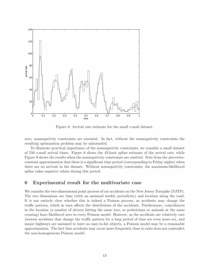
Figure 8: Arrival rate estimate for the small e-mail dataset.

zero, nonnegativity constraints are essential. In fact, without the nonnegativity constraints theresulting optimzation problem may be unbounded.

To illustrate practical importance of the nonnegativity constraints, we consider a small datasetof 550 e-mail arrival times. Figure 8 shows the 42-knot spline estimate of the arrival rate, whileFigure 9 shows the results when the nonnegativity constraints are omitted. Note from the piecewise-constant approximation that there is a significant time period (corresponding to Friday nights) whenthere are no arrivals in the dataset. Without nonnegativity constraints, the maximum-likelihoodspline takes negative values during this period.

6 Experimental result for the multivariate case

We consider the two-dimensional point process of car accidents on the New Jersey Turnpike (NJTP).The two dimensions are time (with an assumed weekly periodicity) and location along the road.It is not entirely clear whether this is indeed a Poisson process, as accidents may change thetraffic pattern, which in turn affects the distribution of the accidents. Furthermore, coincidencesin the location (a number of drivers hitting the same tree, or pedestrians or animals at the samecrossing) have likelihood zero in every Poisson model. However, as the accidents are relatively rare(serious accidents that change the traffic pattern for a long period of time are even more so), andmajor highways are assumed to have no easy-to-hit objects, a Poisson model may be a reasonableapproximation. The fact that accidents may occur more frequently close to exits does not contradictthe non-homogeneous Poisson model.

13

0 0.1 0.2 0.3 0.4 0.5 0.6 0.7 0.8 0.9 1−20

0

20

40

60

80

100

120

140

time

arriv

al r

ate

Figure 9: Estimate for the small e-mail dataset without spline nonnegativity constraints.

The data. We obtained car accident data from the New Jersey Department of Transportation.The raw data contained information on every car accident in 2009 recorded at the accident locationsby police officers. The time of the accident is rounded to the nearest minute, but it is not clearwhether the recorded time is the approximate time of the accident, the time the police were notifiedof the accident, or the time the officers attended to the accident. Hence, we can consider this as noisydata, despite the apparent precision of the time data. The location is given by the Standard RouteIdentifier of the road segment and an approximate milepost reading (variably rounded, apparentlyto the nearest 0.05 mile or to the nearest mile).

We removed all entries from the data that corresponded to accidents in roads other than theNJTP segment marked I-95. This is an approximately 78-mile-long segment stretching betweentwo state borders (with Pennsylvania and New York, respectively) with no forks or joins. Wealso removed entries with missing milepost information. (Date and time were present for everyentry.) While we could take these accidents into account directly in a maximum-likelihood approach(and their time and date information we shall not discard), such incomplete entries were few,and it is reasonable to assume that accidents whose milepost is not recorded follow the samemilepost and time distribution as the entries with complete information, and hence, the removalof this data should not introduce biases. We can then simplify our model, and estimate the arrivalrate based only on the entries with specified milepost, which we can finally multiply with theappropriate constant to account for the discarded accidents. Finally, we removed all accidents thathappened on ramps while entering or leaving the highway, as they are confounding in multipleways. (Unfortunately, this binary flag was missing for most accidents; we assumed that the flagwas false every time it was missing.) Finally, this left us with 4138 accidents.

14

Numerical results. In our example ∆ = [0, T ] × [0,X]; T = 1 week, X = 77.96 miles. Takinginto consideration how the data are rounded, the regions I in the objective function (??) canbe rectangles no smaller than 1 minute by 0.1 miles, but even considerably larger rectangles arereasonable.

Figure 10 shows a biquadratic spline estimator, obtained using the polyhedral inner approxi-mation, with 28× 13 pieces (so each piece corresponds to 6 hours and roughly 6 miles), the regionsI were 1 minute by 1 mile rectangles. The estimator was obtained using an AMPL [FGK02] imple-mentation of Algorithm ??, in which the subproblems were solved by the nonlinear solver KNITRO[NW03]. In this problem there was no clear difference between the biquadratic polyhedral and non-polyhedral WSOS approximations.

Figure 10: A piecewise biquadratic sum-of-squares spline estimator of the NJTP accident rateobtained using Algorithm ??. Left: three-dimensional plot. Right: contour plot. The horizontalaxis shows the time (Monday–Sunday), the vertical axis is location.

7 Conclusion and extension

In this work we have combined ideas from Poisson processes, nonparametric maximum likelihoodestimation, nonnegative polynomials, sum of squares polynomials, and semidefinite programming,to estimate arrival rates of nonhomogeneous Poisson process in both one and two dimensionalcases. In [KSW06] wavelets are used to estimate the (one dimensional) arrival rates. It wouldbe interesting to develop the theory of one and multi-dimensional nonnegative, or sum-of-squareswavelets.

It would also be interesting to look into cases where the arrivals are not quite Poisson, in thatsome interdependence between arrivals may exists. For instance, in e-mail data there may be flamewars where one provocative e-mail, may result in several other e-mails. And in highway accidents, itis possible that one accident, cause backups and traffic jams, where they too cause more accidents.It should be interesting to look into possible autocorrelation in arrival rate function, and model asatisfactory maximum likelihood function model for it.

15

References

[AENR08] F. Alizadeh, J. Eckstein, N. Noyan, and G. Rudolf. Arrival Rate Approximation byNonnegative Cubic Splines . Operations Research, 56(1):140–156, 2008.

[AG03] F. Alizadeh and D. Goldfarb. Second-order cone programming. Math. Program.,95(1):3–51, 2003.

[BH02] Endre Boros and Peter L. Hammer. Pseudo-Boolean optimization. Discrete AppliedMathematics, 123(1–3):155–225, November 2002. doi10.1016/S0166-218X(01)00341-9.

[BHN99] R. M. Byrd, M. E. Hribar, and J. Nocedal. An interior point method for large scalenonlinear programming. SIAM J. Optim., 9(4):877–900, 1999.

[BTN01] Aharon Ben-Tal and Arkadiaei Semenovich Nemirovskiaei. Lectures on modern convexoptimization: analysis, algorithms, and engineering applications. Society for Industrialand Applied Mathematics, Philadelphia, PA, USA, 2001.

[CMM98] J. Czyzyk, M. Mesnier, and J. More. The NEOS server. IEEE J. Comput. Sci. Engrg.,5(3):68–75, 1998.

[Dol01] E. Dolan. The NEOS server 4.0 administrative guide. Technical Report ANL/MCS-TM-250, Mathematics and Computer Science Division, Argonne National Laboratory,Argonne, IL, 2001.

[FGK02] R. Fourer, D. M. Gay, and B. W. Kernighan. AMPL: A Modeling Language for Math-ematical Programming, 2nd edition. Boyd and Fraser, Danvers, MA, 2002.

[GM97] W. Gropp and J. More. Optimization environments and the NEOS server. In M. D.Buhman and A. Iserles, editors, Approximation Theory and Optimization, pages 167–182. Cambridge University Press, Cambridge, UK, 1997.

[KB00] M. E. Kuhl and P. S. Bhairgond. New frontiers in input modeling: nonparametricestimation of nonhomogeneous Poisson process using wavelets. In Proc. 2000 WinterSimulation Conf., pages 562–571, Orlando, FL, 2000.

[KDW97] M. E. Kuhl, H. Damerdji, and J. R. Wilson. Estimating and simulating Poisson processeswith trends or asymmetric cyclic effects. In S. Andradoottir, K. J. Healy, D. H. Withers,and B. L. Nelson, editors, Proceedings of the 1997 Winter Simulation Conference, 1997.

[KSW06] M. E. Kuhl, S. G. Sumant, and J. R. Wilson. An automated multiresolution procedurefor modeling complex arrival processes. INFORMS J. Comput., 18(1):3–18, 2006.

[Mot68] T. Motzkin. The arithmetic-geometric inequalities. In Sisha, O., editor, Inequalities:Proc. Symp. Wright-Patterson AFB, pages 205–224, August 1968.

[Nes00] Y. Nesterov. Squared functional systems and optimization problems. In J. B. G. Frenk,C. Roos, T. Terlaky, and S. Zahng, editors, High Performance Optimization, pages405–440. Kluwer, Dordrecht, The Netherlands, 2000.

[NN94] Y. Nesterov and A. Nemirovski. Interior Point Polynomial Methods in Convex Pro-gramming: Theory and Applications. SIAM, Philadelphia, PA, 1994.

16

[NW03] J. Nocedal and R. A. Waltz. KNITRO user’s manual. Technical Report OTC 2003/05,Optimization Technology Center, Northwestern University, Evanston, IL, 2003.

[PA08] D. Papp and F. Alizadeh. Linear and Second Order Approaches to statistical estima-tion problems. Technical Report RRR 13-08, Rutgers Center for Operations Research,Rutgers University, 2008.

[PA11a] D. Papp and F. Alizadeh. Multivariate Arrival Rate Estimation by Sum-Of-SquaresPolynomial Splines and Semidefinite Programming. Technical Report RRR 5-11, Rut-gers Center for Operations Research, Rutgers University, 2011.

[PA11b] D. Papp and F. Alizadeh. Semidefinite Characterization of Sum-Of-Squares Conesin Algebras. Technical Report RRR 14-11, Rutgers Center for Operations Research,Rutgers University, 2011.

[Sha93] J. Shao. Linear model selection by cross-validation. J. Amer. Statist. Assoc., 88:486–494, 1993.

17