This article was originally published in a journal published byElsevier, and the attached copy is provided by Elsevier for the

author’s benefit and for the benefit of the author’s institution, fornon-commercial research and educational use including without

limitation use in instruction at your institution, sending it to specificcolleagues that you know, and providing a copy to your institution’s

administrator.

All other uses, reproduction and distribution, including withoutlimitation commercial reprints, selling or licensing copies or access,

or posting on open internet sites, your personal or institution’swebsite or repository, are prohibited. For exceptions, permission

may be sought for such use through Elsevier’s permissions site at:

http://www.elsevier.com/locate/permissionusematerial

Autho

r's

pers

onal

co

py

Physics Letters A 367 (2007) 25–34

www.elsevier.com/locate/pla

Coupled-core fluxgate magnetometer: Novel configuration schemeand the effects of a noise-contaminated external signal

Antonio Palacios a, John Aven a, Visarath In b, Patrick Longhini b, Andy Kho b,Joseph D. Neff b, Adi Bulsara b,∗

a San Diego State University, Nonlinear Dynamical Systems Group, Department of Mathematics & Statistics, San Diego, CA 92182-7720, USAb Space and Naval Warfare Systems Center San Diego, Code 2363, 53560 Hull St, San Diego, CA 92152-5001, USA

Received 31 October 2006; received in revised form 3 January 2007; accepted 4 January 2007

Available online 2 March 2007

Communicated by C.R. Doering

Abstract

Recent theoretical and experimental work has shown that unidirectional coupling can induce oscillations in overdamped and undriven nonlineardynamical systems that are non-oscillatory when uncoupled; in turn, this has been shown to lead to new mechanisms for weak (compared tothe energy barrier height) signal detection and amplification. The potential applications include fluxgate magnetometers, electric field sensors,and arrays of Superconducting Quantum Interference Device (SQUID) rings. In the particular case of the fluxgate magnetometer, we have devel-oped a “coupled-core fluxgate magnetometer” (CCFM); this device has been realized in the laboratory and its dynamics used to quantify manyproperties that are generic to this class of systems and coupling. The CCFM operation is underpinned by the emergent oscillatory behavior ina unidirectionally coupled ring of wound ferromagnetic cores, each of which can be treated as an overdamped bistable dynamic system whenuncoupled. In particular, one can determine the regimes of existence and stability of the (coupling-induced) oscillations, and the scaling behaviorof the oscillation frequency. More recently, we studied the effects of a (Gaussian) magnetic noise floor on a CCFM system realized with N = 3coupled ferromagnetic cores. In this Letter, we first introduce a variation on the basic CCFM configuration that affords a path to enhanced devicesensitivity, particularly for N � 3 coupled elements. We then analyze the response of the basic CCFM configuration as well as the new setup to adc target signal that has a small noisy component (or “contamination”).© 2007 Elsevier B.V. All rights reserved.

PACS: 05.45.+b

Keywords: Coupled systems; Fluxgates; Noise; Bistability

1. Introduction

Nonlinear dynamical systems that operate in the vicinity ofa bifurcation point are known to be highly sensitive to smallperturbations; this generic feature has lead to the developmentof new mechanisms for signal detection and amplification. Inthe presence of a noise-floor, these systems display further in-teresting cooperative behavior; a good example is StochasticResonance (SR) wherein the system response to a weak (sub-

* Corresponding author.E-mail addresses: palacios@euler.sdsu.edu (A. Palacios),

visarath@spawar.navy.mil (V. In), bulsara@spawar.navy.mil (A. Bulsara).

threshold) signal can be enhanced by noise of the proper inten-sity to the point where the signal feature in the output powerspectral density becomes observable [1].

Recently, we have discovered that certain coupling schemescan be implemented in arrays of nonlinear dynamic elementsaffording alternative signal detection schemes as well as, po-tentially, enhanced sensitivity. These results have been incorpo-rated into a “coupled core fluxgate magnetometer (CCFM)” [2]and are being exploited to develop an electric field sensor whoseunderlying dynamics are somewhat different [3] from those ofthe dynamic ferromagnetic cores that underpin the CCFM. Thiscoupling scheme has also lead to the prediction of novel coop-erative behavior in a system of coupled SQUID rings [4].

0375-9601/$ – see front matter © 2007 Elsevier B.V. All rights reserved.doi:10.1016/j.physleta.2007.01.089

Autho

r's

pers

onal

co

py

26 A. Palacios et al. / Physics Letters A 367 (2007) 25–34

In this Letter we concentrate on the CCFM as the “test-bed”to demonstrate a variation of our coupling scheme as well as toanalyze the system response to a very weak external symmetry-breaking dc signal that is contaminated by Gaussian noise. Ac-cordingly, a very brief overview of fluxgate magnetometers isprovided here.

Fluxgate magnetometers [5] are considered to be the mostcost-efficient magnetic field sensors for applications that re-quire measuring relatively small magnetic fields in the 0.01 mTregime. Originally developed around 1928, today’s highly spe-cialized devices can measure magnetic fields in the range of1–10 pT/

√Hz [6] for a variety of magnetic remote sensing ap-

plications [7]. In its most basic form, the fluxgate magnetometerconsists of two detection coils wound around two ferromagneticcores (usually a single core configured as an open-ended “race-track”) in opposite directions to one another [5].

The ferromagnetic core that underpins the magnetometer ishysteretic in the core magnetization response to an externalmagnetic field; the dynamics can be modeled via the particle-in-potential paradigm, with the potential energy function beingbistable. In practice, the coercive field (roughly the determin-istic switching threshold between the stable states of the en-ergy function) can be quite high, so that the device shows littleresponse to a target signal of amplitude far smaller than theenergy barrier height. Hence, the standard operating mode con-sists of applying a known time-periodic (usually taken to betriangular or sinusoidal) bias signal, of very large amplitude, toperiodically drive the core between its two stable magnetizationstates. In the absence of the target signal, the power spectraldensity of the output contains only the odd harmonics of the(known) bias frequency. In the presence of a weak (assumednear dc) target signal, however, the potential energy function isskewed, resulting in the appearance of even harmonics; the fre-quency response at the second harmonic is then used to detectand quantify the target signal [5,8].

In our ongoing work (on the single core fluxgate as well asthe CCFM) we rely on a readout mechanism, based on a thresh-old crossing strategy, that consists of measuring the “residencetimes” of the ferromagnetic core(s) in the two stable states ofthe potential energy function [9]. When the potential energyfunction is skewed due to the presence of a target dc signal, theresidence times are no longer equal. Then either their differenceor ratio can be used to quantify the signal. The sensitivity ofthis residence times distribution (RTD) based readout has beenshown [10] to increase with lowered bias frequency and ampli-tude; these conditions are the opposite of the requirements forenhancing sensitivity in traditional (second harmonic) readouts,so that lower onboard power as well as far simpler electronicscan be implemented, with benefit, for this (time domain based)readout strategy [10].

While the CCFM has already been realized in the labora-tory, an analysis of its response to the effects of noise is stillongoing. The problem is complicated by the coupled systemdynamics which, because of the unidirectional coupling, can-not be represented by a (N -dimensional) potential system. Thenoise can also arise in several ways and, in an earlier (numer-ical) analysis [11], we investigated the effects of a noise-floor

(arising, mainly, from the bias signal generator but also fromthe other circuit components) on a CCFM comprised of N = 3unidirectionally coupled ferromagnetic cores.

In this Letter, we now investigate the effects of noise that issuperimposed on (or “contaminates”) a dc target signal, on theresponse of the CCFM. It will become clear that the externalsignal (and its associated noise) are actually part of the argu-ment of the nonlinearity, an effect that can be traced back tothe mean field nature of the magnetics in each core; accord-ingly, we will refer to the noise in this case as “parametricnoise”. The (numerical) analysis suggests that careful tuningof the coupling strength could mitigate the negative effects ofsignal contamination and, simultaneously, it can have the un-expected effect of enhancing the sensitivity of a CCFM-baseddevice.

Additional sensitivity enhancements have been observed,experimentally, when individual cores are oriented in an alter-nating fashion. The foundations of this experimental observa-tion are studied from a theoretical point of view. The studyshows that the coupling-induced oscillations (which underpinthe CCFM concept) are found in essentially the same regionof parameter space as in the standard configuration, where allfluxgates are oriented in the same direction. Interestingly, how-ever, the analysis also points to a sensitivity enhancement bysimply changing the orientation of each individual core; thisis tantamount to alternating the sign of the external signal fromcore to core. More importantly, the sensitivity increases linearlywith the size N of the array. This result is in direct contrast tothe standard configuration in which the sensitivity appears tobe independent of N [2]. The response of this so-called Alter-nating Orientation (AO) configuration to the above-mentionedparametric noise is also a part of our analyses; eventually, wecompare this response to the standard (non-AO) configurationand quantify a regime wherein the AO configuration providessignificantly better response.

We start with an overview of our earlier results for a CCFMcomprised of an odd number N of wound ferromagnetic cores.Note that N (unless taken to be quite large) must be odd. This isfollowed by a (deterministic) description of the AO configura-tion and, finally, a numerical study of the effects of parametricnoise. It should become very clear that the results of this Letter,while confined to the CCFM as a “test-bed”, are applicable toalmost all overdamped bistable dynamic systems. More com-plex behavior is seen in unidirectionally coupled underdampedsystems wherein the interplay between nonlinearity and dissi-pation plays an important role; these systems are the subject ofa future publication.

2. Background

A conventional (i.e., single core) fluxgate magnetometercan be treated as a nonlinear dynamic system by assumingthe core to be approximately single-domain [9], and writingdown an equation for the evolution of the (suitably normalized)macroscopic magnetization parameter x(t): x(t) = −∇xU(x)

in terms of the potential energy function

Autho

r's

pers

onal

co

py

A. Palacios et al. / Physics Letters A 367 (2007) 25–34 27

U(x, t) = x2(t)/2

− c−1 ln cosh c[(x(t) + A sinωt + ε(t)

],

where c is a temperature-dependent nonlinearity parameter,which controls the topology of the potential function: the sys-tem becomes monostable, or paramagnetic, for c < 1 corre-sponding to an increase in the core temperature past the Curiepoint. The overdot denotes the time-derivative, A sinωt is theknown bias signal that switches the core dynamics between thepotential minima, and ε(t) is an external target signal (taken tobe dc throughout this treatment).

The CCFM is, then, constructed by unidirectionally couplingN (odd) wound ferromagnetic cores with cyclic boundary con-dition, thereby leading to the dynamics,

xi = −xi + tanh(c(xi + λxi+1 + ε)

),

(1)i = 1, . . . ,N mod N,

where xi(t) represents the (suitably normalized) magnetic fluxat the output (i.e., in the secondary coil) of unit i, and ε � U0is an external dc “target” magnetic flux, U0 being the energybarrier height (absent the coupling) for each of the elements (as-sumed identical for theoretical purposes). It is important to note[2] that the oscillatory behavior occurs even for ε = 0, how-ever when ε �= 0, the oscillation characteristics change; thesechanges can be exploited for signal quantification purposes, themotivation for this work. We reiterate that the oscillations donot occur for λ = 0 due to the overdamped nature of the dynam-ics (1). Note the absence of the bias signal in the dynamics (1);in the coupled core system, the oscillations (corresponding toswitching events in each core between the allowed stable states)are generated by the coupling and the cyclic boundary condi-tion. In an experimental setup, there is always a power supply inthe circuit to drive the electronic components that make up, e.g.,the coupling circuit, so that the oscillations do not violate anyfundamental laws. We also observe that the particle-in-potentialparadigm is no longer applicable to the coupled system (1) dueto the unidirectional coupling. The above system (with N = 3)has been realized in the laboratory [2] and is, currently beingimplemented in a cheap, lightweight, low-power magnetic sen-sor.

A theoretical analysis [2] shows that the system (1) exhibitscoupling-induced oscillatory behavior with the following fea-tures:

(1) The oscillations commence when the coupling coeffi-cient exceeds a threshold value

λc = −ε − xinf + c−1 tanh−1 xinf,

with xinf = √(c − 1)/c; note that in our convention, λ < 0 so

that oscillations occur for |λ| > |λc|.(2) The individual oscillations (in each elemental response)

are separated in phase by 2π/N , and have period

Ti = Nπ(1/

√λc − λ + 1/

√λc − λ + 2ε

)/√

cxinf,

which shows a characteristic dependence on the inverse squareroot of the bifurcation “distance” λc − λ, as well as the targetsignal ε; these oscillations can be experimentally produced atfrequencies ranging from a few Hz to high kHz.

Fig. 1. Simulated frequency response of a CCFM in the absence of noise. Para-meters are: N = 3 cores and c = 3.

(3) The summed output oscillates at period T+ = Ti/N andits amplitude (as well as that of each elemental oscillation) isalways suprathreshold, i.e., the emergent oscillations are strongenough to drive each core between its saturation states, elimi-nating the need to apply an additional bias signal. Increasing N

changes the frequency of the individual elemental oscillations,but the frequency of the summed response is seen to be inde-pendent of N . Fig. 1 shows the relation between the frequencyresponse of coupling-induced oscillations in the system (1) withN = 3 cores, and c = 3, as a function of the coupling strengthλ and the intensity of the target signal ε. The characteristic(square root) scaling is well-satisfied. As expected, decreas-ing the coupling strength increases the oscillation frequency.Changing the target field strength also changes the frequency.In practice, however, it is usually more convenient to use theresidence times difference (RTD) �t as a quantifier of the tar-get signal.

(4) The RTD can be computed as

�t ≈ π(1/

√λc − λ − 1/

√λc − λ + 2ε

)/√

cxinf,

which vanishes (as expected) for ε = 0, and can be used as aquantifier of the target signal, analogous to the time-domain op-eration of the single fluxgate [9].

(5) The system responsivity, defined via the derivative∂�t/∂ε, is found to increase dramatically as one approachesthe critical point in the oscillatory regime; this suggests thatcareful tuning of the coupling parameter so that the oscillationshave very low frequency, could offer significant benefits for thedetection of very small target signals. For small target signals,one may do a small-ε expansion to yield

�t ≈ πε(λc0 − λ)−3/2/√

cxinf,

where λc0 now represents the critical coupling, absent the targetsignal. For a fixed ε, one observes, immediately, that the respon-sivity ∂�t/∂ε increases as one approaches the critical point(through adjusting the coupling parameter λ). The instrumentthus yields its optimal performance in the very low frequencyregime, close to the oscillation threshold; it is worth noting thatthe experimental system can be made to oscillate at very low

Autho

r's

pers

onal

co

py

28 A. Palacios et al. / Physics Letters A 367 (2007) 25–34

frequencies (around 65 Hz), far lower than the bias frequencyfor conventional fluxgates. The coupled system can be “tuned”to this regime by adjusting the coupling coefficient λ. This “tun-ability” of the optimal operating regime, if done carefully withconsideration of the magnitude of target signals expected in agiven application, is a big advantage (in addition to the absenceof the bias signal) of the coupled system over its single elementcounterpart. In conventional fluxgate magnetometers, the biassignal generator is, usually, a major source of noise in the sys-tem, since it must produce a signal of high amplitude (muchgreater than the energy barrier) and very high frequency (typ-ically 30–200 kHz). This function also requires a significantonboard power supply. Coupling, therefore, allows one to ex-ploit the target-signal dependence of the emergent oscillationsfor detection and quantification purposes. It is important to real-ize that, in the coupled system, the assorted circuit components(in particular those that realize the coupling circuit) do requirean onboard power source (although, typically, less than that re-quired in a conventional setup); hence the emergence of theoscillations does not violate any fundamental laws.

3. A new configuration for the CCFM

Laboratory experiments seem to indicate that the sensitivityof a CCFM-based system of fluxgates increases by simply alter-nating the orientation of each individual fluxgate. We call thisnew arrangement a CCFM system with Alternating Orienta-tion (AO). We should clarify that the coupling scheme remainsthe same, i.e., unidirectional coupling via induction. The onlyfeature that changes is the direction at which the individual flux-gates are aimed for signal detection purposes. Thus the sign infront of the target signal ε alternates between + and − so thatthe governing equations (for the deterministic system) become,

xi = −xi + tanh(c(xi + λxi + (−1)i+1ε

)),

(2)i = 1, . . . ,N mod N.

Next we calculate the region of existence of stable coupling-induced oscillations using the ideas and methods from our pre-vious work on the analysis of the standard CCFM configuration[2]. Without loss of generality, we consider the particular caseof N = 3 cores. In the absence of noise and of a target sig-nal, i.e., ε = 0, Eq. (2) reduces to that of the standard CCFMsystem (1). Hence the one-parameter bifurcation of xi vs. λ

remains the same: the coupling-induced oscillations exist onlywhen N is odd and for λ < λAO

c , where λAOc is a critical thresh-

old value of coupling strength and the superscript denotes thetype of configuration. The two-parameter bifurcation of xi vs.(λ, ε) might be, however, different since the signs in front ofthe input signal are now different. Thus we seek to determineλAO

c as a function of ε. Computer simulations of (2) show that,as in the case of the standard CCFM system, the oscillationsemerge via global bifurcations of a heteroclinic cycle connect-ing six saddle-node equilibrium points: (1,−1,−1), (1,1,−1),(−1,1,−1), (−1,1,1), (−1,−1,1), and (1,−1,1). Further-more, solution trajectories are confined (as is typically the casewith heteroclinic cycles) to the intersection of certain invariant

planar regions given by (with λ < 0):

δi = {xi : λxi < 1, x(i+2 mod 3) = −1},i = 1,2,3,

δi = {xi : λxi > −1, x(i+2 mod 3) = 1},i = 4,5,6.

The saddle-node points exist only for λ > λAOc and are annihi-

lated when the periodic solutions appear. This suggests that wecould determine the exact location of the heteroclinic cycle byfinding the regions of parameter space where the saddle pointsexist, but this approach would involve the complicated task offinding roots of polynomials of high order. On the other hand,we can use the fact that, at the birth of the cycle, solutions areconfined to invariant lines. The flow on these lines cannot beobstructed by other equilibrium points, unless they are part ofthe cycles. This leads to the following conditions for existenceof a cyclic solution:

(3)−x + tanh(c(x − λ + ε)

)> 0,

(4)−x + tanh(c(x − λ − ε)

)> 0,

(5)−x + tanh(c(x + λ + ε)

)< 0,

(6)−x + tanh(c(x + λ − ε)

)< 0.

When ε = 0, the inequalities (3) and (6) are satisfied for allvalues of x and λ. On increasing ε, the graph of the left-handside of (3) shifts vertically upward while that of the left-handside of (6) shifts vertically downward. Thus both inequalities(3) and (6) are satisfied for all ε � 0. Recalling that ε repre-sents the external signal which we assume to be nonnegative,we now consider the conditions (4) and (5). Direct calculationsshow that the solution set, on the plane (λ, ε), for (5) is includedin that of (4) but not the other way around. Consequently, to findthe critical point λAO

c where the oscillations commence, we onlyneed to solve (5). This condition was already solved in our pre-vious work [2]. Here, we repeat the calculation (which is verybrief) for completeness. The graph of the left-hand side of (5)shows a local minimum and a local maximum for x ∈ (−1 : 1).Oscillations commence when the local maximum crosses zero.Thus we compute the maximum, set it equal to zero, and solvefor λ to get

λAOc = −ε + 1

cln

(√c + √

c − 1)

(7)− tanh(ln

(√c + √

c − 1) )

.

Eq. (7) describes the onset of oscillations in the CCFM sys-tem with AO configuration. This onset is exactly the same asthat of the standard configuration. Interestingly, the AO config-uration does not change the two-parameter region where stablecoupling-induced oscillations exist. More interesting, however,is the fact that the sensitivity response of the AO configurationdoes change. Actually, it improves significantly in our experi-mental observations, a claim that we now approach analytically.We do so by calculating the RTD response of an AO configura-tion with the aid of time-series simulations of typical solutiontrajectories for xi(t); these solutions are shown in Fig. 2. From

Autho

r's

pers

onal

co

py

A. Palacios et al. / Physics Letters A 367 (2007) 25–34 29

Fig. 2. Time series simulations of a CCFM system with cores oriented in an al-ternating fashion. Parameters are: N = 3 cores, c = 3, λ = −0.54, and ε = 0.07.The time intervals ti are used (see text) in the calculation of the period and RTD.

Fig. 2, we observe that on the interval t1 the dominant part ofx3(t) decreases from 1 (the approximate location of the fixedpoint of the “local” potential U(x1)) absent any coupling) to0 (the maximum of the local potential) while the element x1(t)

remains in its steady state x+ ≈ 1 (the exact locations of the sta-ble fixed points of each local potential can be readily found viasimple calculus [2] and, for c > 1, are very close to ±1, due tothe tanh function) so that the last of Eqs. (2) (with N = 3) canbe simplified to:

(8)x3(t) = −x3 + tanh c(x3 + λ + ε),

corresponding to simple “particle-in-potential” motion. It is im-portant to note that, because of the sequential nature of theswitching process one can reduce the dynamics to a descrip-tion in terms of a “local” potential, even though the 3-variablecoupled system cannot be described by a potential energy func-tion. Formally integrating this equation yields,

(9)t1 =0∫

1

dx3

tanh c(x3 + λ + ε) − x3,

where t1 is the time taken (for this choice of initial conditions)by the state-point x3(t) to evolve from its stable attractor at+1, to 0 (Fig. 2). This integral cannot be evaluated analytically,in general. However, it may be evaluated just past the criticalpoint (i.e., in the regime of low oscillation frequency), wherethe integrand is sharply peaked. We note that the denomina-tor is sharply peaked at x3 = xm3, a value that can be foundby differentiation as xm3 = −λ − ε + (1/c) tanh−1 xinf, wherexinf = √

(c − 1)/c. The critical coupling at which the potentialfunction U(x3) corresponding to the x3 dynamics has an inflec-tion point, may be obtained by setting f (xinf, λc3) = 0, f (x,λ)

being the denominator in the integrand of (9). We readily ob-tain,

(10)λc3 = −ε − xinf + 1

ctanh−1 xinf,

so that xm3 = λc3 − λ + xinf. We now expand the denominatorf (x3) about x3 = xm3 obtaining, after some algebra,

f (x3) ≡ tanh c(x3 + λ + ε) − x3

(11)≈ λ − λc3 − cxinf(x3 − xm3)2.

Then, finally, we can evaluate the integral in (9), extending thelimits to ±∞ (because of the sharply peaked nature of the inte-grand):

t1 ≈∞∫

−∞

dx3

λc3 − λ + cxinf(x3 − xm3)2

(12)= π√cxinf

√λc3 − λ

.

Next we calculate the interval t2. Fig. 2 shows that, on t2, thedynamics along x2(t) changes while x3 ≈ −1 so that

(13)x2(t) = −x2 + tanh c(x2 − λ − ε),

which yields

(14)t2 =0∫

−1

dx2

tanh c(x2 − λ − ε) − x2.

Proceeding as in the t1 case, we find that t2 is, approximately,given by

(15)t2 ≈∞∫

−∞

dx2

λc2 − λ + cxinf(x2 + xm2)2.

It can be shown that xm2 = −xm3 while the critical couplingλc2 is the same as in the t1 case, i.e., λc2 = λc3. It follows thatt2 = t1. In fact, similar calculations also show that t1 = t2 = t3.

To calculate t4, we observe (see Fig. 2) that, on this interval,the dominant part of x3(t) increases from −1 to 0 while the ele-ment x1(t) remains in its steady state x− ≈ −1, so the behaviorof x3 is well approximated by

(16)x3(t) = −x3 + tanh c(x3 − λ + ε),

which yields

(17)t4 =0∫

−1

dx3

tanh c(x3 − λ + ε) − x3.

Once again, we can show that the critical coupling at whichthe local potential function U(x3) (dynamics restricted to theinterval t4) has an inflection point is given by

(18)λc33 = ε − xinf + 1

ctanh−1 xinf.

Direct calculations also show that the denominator of (17) issharply peaked at xm33 = λ − λc33 − xinf. Then we expand thisdenominator about xm33 to get

tanh c(x3 − λ + ε) − x3

(19)≈ λc33 − λ − cxinf(x3 − xm33)2.

Autho

r's

pers

onal

co

py

30 A. Palacios et al. / Physics Letters A 367 (2007) 25–34

Using the relation λc33 = λc3 + 2ε, we finally arrive at an ex-pression for t4

t4 ≈∞∫

−∞

dx3

λc3 − λ + 2ε + cxinf(x3 + xm33)2

(20)= π√cxinf

√λc3 − λ + 2ε

.

In addition, we can show that t4 = t5 = t6. Thus we may nowwrite down the oscillation periods, Ti , i = 1,2,3, of the indi-vidual waveforms in terms of t1 and t4. After some algebra wefind that T1 = 3(t1 + t4) and the other two periods are identi-cal, i.e., T1 = T2 = T3. Using the integral approximations to t1and t4, Eq. (12) and Eq. (20), respectively, we arrive at

(21)Ti = 3π√cxinf

[1√

λc3 − λ+ 1√

λc3 − λ + 2ε

].

We note that this last equation is identical to the one that de-scribes the period of the individual output signals of the stan-dard configuration. However, as we will show next, the Resi-dence Times Difference (RTD) for the AO configuration is dif-ferent depending on the element under consideration, as readilyapparent in Fig. 2. Using Fig. 2 as a reference, we may alsowrite down the RTDs for all three waveforms in terms of t1and t4. This leads to �1t = 3(t1 − t4) and �2t = �3t = t1 − t4,corresponding, respectively, to the signals xi(t) (i = 1 − 3).Clearly, the waveform x1(t) is more sensitive (to small changesin the dc target signal) than the other two outputs by a factorof 3. From (12) and (20), respectively, we then obtain a closed-form expression for the RTD using x1 as a detection signal:

(22)�1t = 3π√cxinf

[1√

λc3 − λ− 1√

λc3 − λ + 2ε

].

This last equation reveals that the sensitivity of x1(t) in the AOconfiguration is exactly three times the best sensitivity responsethat can be achieved by the standard configuration. We notethat, in the latter case, the RTDs corresponding to all the outputwaveforms are identical and they are, moreover, identical to theRTD obtained via the summed output. The above-demonstratedimprovement in the RTD for the AO case is even better forlarger networks as we demonstrate next.

The generalization of the above observations to rings of ar-bitrary size N is straightforward. Similar computer simulationsand calculations show that there are now N intervals of size t1and N intervals of size tN+1. The period Ti , i = 1, . . . ,N , of theindividual signals are all the same: Ti = N(t1 + TN+1). Usingsignal x1(t), the RTD is �1t = N(t1 − tN+1). For the remainingsignals the RTD is �j t = t1 − tN+1 = (1/N)�1, j = 2, . . . ,N .Direct calculations of t1 and TN+1 then lead to the followinganalytic results:

(23)Ti = Nπ√cxinf

[1√

λc3 − λ+ 1√

λc3 − λ + 2ε

],

and,

(24)�1t = Nπ√cxinf

[1√

λc3 − λ− 1√

λc3 − λ + 2ε

].

Recall that ∂�t/∂ε measures the sensitivity of a CCFM (in thestandard orientation). It follows that

∂�1t

∂ε= N

∂�t

∂ε.

In other words, the sensitivity of the AO configuration, usingx1(t) as the detecting signal, improves, linearly, by a factor of N

when is compared to the best sensitivity that can be achieved bythe summed output signal of the standard configuration, giventhe same external signal and core parameters. The dependenceof the RTD, and consequently of the sensitivity, on the size ofthe ring in the AO configuration is in direct contrast to the sensi-tivity response of the standard configuration, in which increas-ing N beyond N = 3 does not lead to additional benefits. Weshould emphasize that the standard configuration, nevertheless,still outperforms the sensitivity of a magnetometer based on asingle uncoupled core. The above observations are confirmed inFig. 3, in which we calculate, numerically, the RTD �1t for aCCFM system with standard as well as with AO configuration.As expected, near the onset of coupling-induced oscillations,the RTD response of the standard configuration remains con-stant while that of the AO configuration increases, linearly, asa function of N . The RTDs were calculated using the summedoutput signal

∑xi(t) for the standard configuration (as already

Fig. 3. RTD response of a CCFM as a function of ring size N and of coupling strength λ. (Left) standard configuration and (right) AO configuration. Near the onsetof coupled-induced oscillations, in particular, the RTD response of the standard configuration remains constant (as expected) while that of the AO configurationincreases linearly as a function of N . c = 3, ε = 0.

Autho

r's

pers

onal

co

py

A. Palacios et al. / Physics Letters A 367 (2007) 25–34 31

mentioned, this RTD is identical to that obtained via individ-ual elements for the standard configuration), and the individualsignal x1(t) for the AO configuration.

It is clear that, for rings of arbitrary odd N elements, onealways has a situation wherein two adjacent elements have thesame orientation (i.e., the sign of the dc term in the dynamics(2) is the same for these two elements). In this case, the mostsensitive (in the RTD) element is always the one (out of thesetwo elements) which is forward coupled to an element with theopposite orientation. For example, in the system at hand, x3 andx1 have the same orientation, with x3 forward coupled to x1(same orientation) but x1 forward coupled to x2 (opposite ori-entation); hence x1 is the most sensitive for detecting the targetdc signal via the RTD. The effect of the AO configuration on thesensitivity seems to be universal for other sensor systems thatare underpinned by unidirectionally coupled bistable element,e.g., the behavior can be predicted theoretically, and verified viasimulations in an electric field sensor [3] which is realized byunidirectionally coupling N ferroelectric core elements which,whilst being bistable, have potential energy functions quite dif-ferent in structure to the ferromagnetic case treated here.

4. Target signal contamination by noise

We expect noise in our CCFM to arise from three sources:a magnetic noise floor (due to the core material and, in par-ticular, magnetic domain motion), contamination of the targetsignal, and noise from the electronics in the coupling circuitry.In recent work we studied, numerically, the effects of an addi-tive magnetic noise floor [11]. We now investigate the case ofa target signal contaminated by noise, assumed to be Gaussianband-limited noise having zero mean, correlation time τc, andvariance σ 2. This type of noise is a good approximation (except

for a small 1/f component at very low frequencies) to what isactually observed in the experimental setup. From a modelingpoint of view, colored noise η(t) that contaminates the signalshould appear now as an additive term inside the tanh functionof Eq. (1), i.e.,

dxi

dt= −xi + tanh

(c(xi + λxi+1 + ε + ηi(t)

)),

(25)dηi

dt= −ηi

τc

+√

2D

τc

ξ(t).

In general, we would expect somewhat different noise in eachequation, since, realistically, the reading of the external signalε is slightly different in each core. This is due to non-identicalcircuit elements and cores, mainly. In this work we will con-sider, therefore, the situation wherein the different noise termsηi(t) are uncorrelated; however, for simplicity, we will assumethem to have the same intensity D. Each (colored) noise ηi(t)

is characterized by 〈ηi(t)〉 = 0 and 〈ηi(t)ηi(s)〉 = (D/τc) ×exp [−|t − s|/τc], where D = σ 2τ 2

c /2 is the noise intensity, andthe “white” limit is obtained for vanishing τc; in practice, how-ever, the noise is always band-limited. In this formulation, weassume the signal to be contaminated purely by external noise;in future work, however, we will also consider other sources ofcontamination such as internal noise introduced by each indi-vidual core, as well as the coupling and readout circuits.

We assume the temperature-related parameter c to be con-stant throughout. Throughout our simulations, we take the tar-get signal to be ε = 0.07, well below the energy threshold ofa single (uncoupled) core. Of course, the results are expectedto be similar to those found at other values of the target signalwithin the energy barrier height.

Fig. 4 shows the relation between the mean oscillation fre-quency of (a single core element of) the CCFM with N = 3

Fig. 4. Frequency (Hz) response of simulations of a CCFM system, subject to parametric noise, as a function of coupling strength λ and noise intensity D. Parametersare: N = 3 cores, c = 3, τc = 150, and ε = 0.07. SO denotes the standard orientation in which all individual fluxgates are similarly oriented for signal detectionpurposes. Observe that the onset of coupling-induced oscillations shifts slightly (to the left of λc) for larger values of noise intensity, as is shown by the small dentin the surface plot near D = 0.5.

Autho

r's

pers

onal

co

py

32 A. Palacios et al. / Physics Letters A 367 (2007) 25–34

Fig. 5. Signal-to-Noise-Ratio output of (a single element) of a CCFM system in the presence of parametric noise. Parameters are: N = 3 cores, c = 3, τc = 150.0,and ε = 0.07.

cores and the system parameters (coupling strength λ and noiseintensity D). The mnemonic “SO” in the figure stands for stan-dard orientation, in which all the individual cores have the samespatial orientation (i.e., the sign of the target signal term is thesame in each equation of the system (25)) for signal detectionpurposes. A sample of one thousand time-series simulationswas then used to compute the frequency output at each pointin parameter space (λ,D). Each simulation was carried outwith correlation time set to τc = 150 since typically τF � τc,where τF = 1 is the time constant of the core dynamics givenby (1). Observe that the critical-coupling bifurcation point λc ofthe deterministic system, i.e., D = 0, remains, approximately,unchanged for small values of noise intensity. There is, how-ever, a subtle shift in the bifurcation point for increasing noise(beyond D = 0.25). The noise appears to have the effect of de-laying the onset of oscillatory behavior. We find (not shown)that the delay is less pronounced in the more idealized scenarioin which the noise ηi(t) is taken to be the same in each core.Next we study the response of the CCFM through the Signal-to-Noise-Ratio (SNR). Fig. 5 shows the SNR (of the outputof a single core element) in the same parameter space (λ,D).The SNR increases rapidly near the critical coupling, as wewould expect. The negative effects of highly contaminated sig-nals (large noise intensity) appear to be well-mitigated by thesensitivity response of the system. To the right of the onset ofoscillatory behavior, where the global dynamics of the deter-ministic system typically settle into a steady-state equilibrium,we now observe small fluctuations in the SNR caused mainlyby noise. These fluctuations get smaller as the number of simu-lation samples increases.

It is worth mentioning that these small fluctuations are alsopresent in the more ideal case wherein we take identical noisefunctions in each element of the dynamics. We now investigatethe AO configuration which, as suggested by the results of thepreceding section, as well as our laboratory experiments, holds

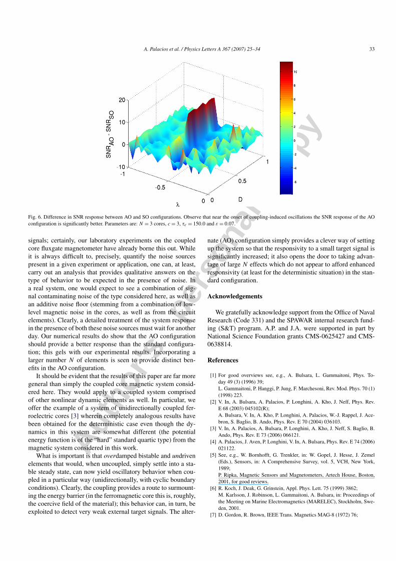
out the promise of further performance enhancements. Finally,we study the effects of noise on the CCFM with the AO config-uration. We use the output of the “favored” element that givesthe best deterministic RTD response (see preceding section) inthis configuration. Calculations of the SNR output of this “fa-vored” element (not shown for brevity) show, at first glance,similar results to those of the standard-orientation configura-tion. A point-wise comparison between the SNR output of thetwo cases indicates, however, that the SNR output of (the fa-vored element of) the AO configuration can be larger than thatof the standard (CCFM) system (Fig. 6). Near the critical cou-pling strength, in particular, the SNR response of the AO systemappears to be significantly better than that of the standard con-figuration. Large coupling strengths, on the contrary, reduce theSNR response of the AO configuration to values that are com-parable to those of the standard case. The improvement in SNRoutput of the AO configuration over the standard (SO) case isalso present in the ideal case of identical noises in the cores;however, in this case, the improvement occurs for smaller val-ues of noise intensity. In both cases, non-identical and identicalnoise terms, the difference between the SNR outputs suggeststhat careful tuning of the coupling strength can mitigate the neg-ative effects of signal contamination so that full advantage canbe taken of the sensitivity enhancements of a CCFM systemwith AO configuration.

5. Discussion

In this Letter, we have expanded our earlier ideas of cou-pling overdamped nonlinear dynamic elements in a carefullychosen configuration, so that the emergent oscillations that oc-cur when a control parameter exceeds a threshold value can beused as an identifier of small symmetry breaking target signals.The alternate (AO) configuration points to a variation of our ba-sic scheme that can lead to greatly enhanced sensitivity to small

Autho

r's

pers

onal

co

py

A. Palacios et al. / Physics Letters A 367 (2007) 25–34 33

Fig. 6. Difference in SNR response between AO and SO configurations. Observe that near the onset of coupling-induced oscillations the SNR response of the AOconfiguration is significantly better. Parameters are: N = 3 cores, c = 3, τc = 150.0 and ε = 0.07.

signals; certainly, our laboratory experiments on the coupledcore fluxgate magnetometer have already borne this out. Whileit is always difficult to, precisely, quantify the noise sourcespresent in a given experiment or application, one can, at least,carry out an analysis that provides qualitative answers on thetype of behavior to be expected in the presence of noise. Ina real system, one would expect to see a combination of sig-nal contaminating noise of the type considered here, as well asan additive noise floor (stemming from a combination of low-level magnetic noise in the cores, as well as from the circuitelements). Clearly, a detailed treatment of the system responsein the presence of both these noise sources must wait for anotherday. Our numerical results do show that the AO configurationshould provide a better response than the standard configura-tion; this gels with our experimental results. Incorporating alarger number N of elements is seen to provide distinct ben-efits in the AO configuration.

It should be evident that the results of this paper are far moregeneral than simply the coupled core magnetic system consid-ered here. They would apply to a coupled system comprisedof other nonlinear dynamic elements as well. In particular, weoffer the example of a system of unidirectionally coupled fer-roelectric cores [3] wherein completely analogous results havebeen obtained for the deterministic case even though the dy-namics in this system are somewhat different (the potentialenergy function is of the “hard” standard quartic type) from themagnetic system considered in this work.

What is important is that overdamped bistable and undrivenelements that would, when uncoupled, simply settle into a sta-ble steady state, can now yield oscillatory behavior when cou-pled in a particular way (unidirectionally, with cyclic boundaryconditions). Clearly, the coupling provides a route to surmount-ing the energy barrier (in the ferromagnetic core this is, roughly,the coercive field of the material); this behavior can, in turn, beexploited to detect very weak external target signals. The alter-

nate (AO) configuration simply provides a clever way of settingup the system so that the responsivity to a small target signal issignificantly increased; it also opens the door to taking advan-tage of large N effects which do not appear to afford enhancedresponsivity (at least for the deterministic situation) in the stan-dard configuration.

Acknowledgements

We gratefully acknowledge support from the Office of NavalResearch (Code 331) and the SPAWAR internal research fund-ing (S&T) program. A.P. and J.A. were supported in part byNational Science Foundation grants CMS-0625427 and CMS-0638814.

References

[1] For good overviews see, e.g., A. Bulsara, L. Gammaitoni, Phys. To-day 49 (3) (1996) 39;L. Gammaitoni, P. Hanggi, P. Jung, F. Marchesoni, Rev. Mod. Phys. 70 (1)(1998) 223.

[2] V. In, A. Bulsara, A. Palacios, P. Longhini, A. Kho, J. Neff, Phys. Rev.E 68 (2003) 045102(R);A. Bulsara, V. In, A. Kho, P. Longhini, A. Palacios, W.-J. Rappel, J. Ace-bron, S. Baglio, B. Ando, Phys. Rev. E 70 (2004) 036103.

[3] V. In, A. Palacios, A. Bulsara, P. Longhini, A. Kho, J. Neff, S. Baglio, B.Ando, Phys. Rev. E 73 (2006) 066121.

[4] A. Palacios, J. Aven, P. Longhini, V. In, A. Bulsara, Phys. Rev. E 74 (2006)021122.

[5] See, e.g., W. Bornhofft, G. Trenkler, in: W. Gopel, J. Hesse, J. Zemel(Eds.), Sensors, in: A Comprehensive Survey, vol. 5, VCH, New York,1989;P. Ripka, Magnetic Sensors and Magnetometers, Artech House, Boston,2001, for good reviews.

[6] R. Koch, J. Deak, G. Grinstein, Appl. Phys. Lett. 75 (1999) 3862;M. Karlsson, J. Robinson, L. Gammaitoni, A. Bulsara, in: Proceedings ofthe Meeting on Marine Electromagnetics (MARELEC), Stockholm, Swe-den, 2001.

[7] D. Gordon, R. Brown, IEEE Trans. Magnetics MAG-8 (1972) 76;

Autho

r's

pers

onal

co

py

34 A. Palacios et al. / Physics Letters A 367 (2007) 25–34

C. Russell, R. Elphic, J. Slavin, Science 203 (1979) 745;J. Lenz, IEEE Proc. 78 (1990) 973;R. Snare, J. Means, IEEE Trans. Mag. MAG-13 (1997) 1107.

[8] F. Primdahl, J. Phys. E 12 (1979) 241;P. Ripka, Sensors Actuators A 33 (1992) 129;P. Ripka, Sensors Actuators A 106 (2003) 8.

[9] A. Bulsara, C. Seberino, L. Gammaitoni, M. Karlsson, B. Lundqvist,J.W.C. Robinson, Phys. Rev. E 67 (2003) 016120.

[10] B. Ando, S. Baglio, A. Bulsara, V. Sacco, in: Proceedings of the 24thIEEE Instrumentation and Measurement Conference, Como, Italy (2004)Pg. 1419;B. Ando, S. Baglio, A. Bulsara, V. Sacco, Measurement 38 (2005) 89;B. Ando, S. Baglio, A. Bulsara, V. Sacco, IEEE Sensors 5 (2005) 895.

[11] A. Bulsara, J. Lindner, V. In, A. Kho, S. Baglio, V. Sacco, B. Ando, P.Longhini, A. Palacios, W. Rappel, Phys. Lett. A 353 (2006) 4.