
Power System Oscillations -- Detection Estimation and Control
159
Power System Oscillations - Detection, Estimation and Control Hemmingsson, Morten 2003 Link to publication Citation for published version (APA): Hemmingsson, M. (2003). Power System Oscillations - Detection, Estimation and Control. Department of Industrial Electrical Engineering and Automation, Lund Institute of Technology. Total number of authors: 1 General rights Unless other specific re-use rights are stated the following general rights apply: Copyright and moral rights for the publications made accessible in the public portal are retained by the authors and/or other copyright owners and it is a condition of accessing publications that users recognise and abide by the legal requirements associated with these rights. • Users may download and print one copy of any publication from the public portal for the purpose of private study or research. • You may not further distribute the material or use it for any profit-making activity or commercial gain • You may freely distribute the URL identifying the publication in the public portal Read more about Creative commons licenses: https://creativecommons.org/licenses/ Take down policy If you believe that this document breaches copyright please contact us providing details, and we will remove access to the work immediately and investigate your claim.
-
Upload
khangminh22 -
Category
Documents
-
view
4 -
download
0
Transcript of Power System Oscillations -- Detection Estimation and Control

LUND UNIVERSITY
PO Box 117221 00 Lund+46 46-222 00 00
Power System Oscillations - Detection, Estimation and Control
Hemmingsson, Morten
2003
Link to publication
Citation for published version (APA):Hemmingsson, M. (2003). Power System Oscillations - Detection, Estimation and Control. Department ofIndustrial Electrical Engineering and Automation, Lund Institute of Technology.
Total number of authors:1
General rightsUnless other specific re-use rights are stated the following general rights apply:Copyright and moral rights for the publications made accessible in the public portal are retained by the authorsand/or other copyright owners and it is a condition of accessing publications that users recognise and abide by thelegal requirements associated with these rights. • Users may download and print one copy of any publication from the public portal for the purpose of private studyor research. • You may not further distribute the material or use it for any profit-making activity or commercial gain • You may freely distribute the URL identifying the publication in the public portal
Read more about Creative commons licenses: https://creativecommons.org/licenses/Take down policyIf you believe that this document breaches copyright please contact us providing details, and we will removeaccess to the work immediately and investigate your claim.

Power System OscillationsDetection Estimation & Control
Morten Hemmingsson
Doctoral Dissertation in Industrial AutomationDepartment of Industrial Electrical Engineering
and Automation

Department ofIndustrial Electrical Engineering and AutomationLund Institute of TechnologyLund UniversityP.O. Box 118S-221 00 LUNDSWEDEN
http://www.iea.lth.se
ISBN 91-88934-27-6CODEN:LUTEDX/(TEIE-1035)/1-158/(2003)
c©Morten HemmingssonPrinted in Sweden by Universitetstryckeriet, Lund University

Abstract
The topic of this thesis is the electro-mechanical oscillations which to some ex-tent always are present in a power system. The demand of electric power is everincreasing. At the same time, the tolerance of disruptions in the power sup-ply is decreasing. The deregulated market together with distributed generationhave then pushed the system to operate during circumstances for which it wasnot designed. To this we can then add that getting concessions for new linesbecomes more and more difficult in densly populated areas. All these factorsmakes the electric power system operate with smaller safety margins. Decreas-ing these margins limits with sustained availability is achieved by the applicationof advanced monitoring and control methods.
This thesis deals with this in several time-scales. When a large oscillationoccurs it is important to detect it as fast as possible as the remedial action de-pends on if the current operating is due to a fault or an oscillation. In the thesis,a new method to distinguish these incidents from each other is presented.
In a slower time-scale it is important to monitor the dynamics of the electro-mechanical modes. This information can be used to verify that simulationscorrespond to the real world behaviour. Real-time methods can also be used toalarm operators or arm special protection schemes if the power system entersundesired operating conditions. A number of methods are studied and thenevaluated on three case studies.
Finally, load modulation for damping enhancement is studied. It has pre-viously been shown that modulation of active power at the transmission levelincreases the damping of the power system when correctly performed. Loadssuitable for load modulation at the transmission level are rare and using actuat-ors at the distribution level creates new problems. It is shown that it is possibleto detect poor damping at the distribution level, thus reducing the need of com-munications. It is also shown how the variation of active and reactive power at
iii

the transmission level, caused by modulation of active power at the distribu-tion level can be estimated without knowledge of the complete distributionnetwork. This is most important as the active and reactive variations counteracteach other. Finally load modulation at distribution level is evaluated on twotest systems. It is shown that the damping is increased and that the influenceof the reactive variation decreases the performance of load modulation. Thedegradation of the control scheme is, however, small in the studied cases.
iv

Acknowledgements
This thesis, although written by me, would not have been possible withoutthe cooperation and aid of several persons. My supervisors, Gustaf Olsson andOlof Samuelsson deserves a great thank for guiding me through the traps andpitfalls of research. Gustaf ’s open mind and vast knowledge of various fields isinvaluable when working in the cross-lands of different areas. His reading ofthe manuscript has also improved the final product a lot. Olof was the one whointroduced me to power systems and showed me that it could be so much morethan asymmetric faults in phase quantities. I also appreciate his view that resultsshould be possible to explain by using the basic mechanisms behind differentphenomena. Both of them has been invaluable for keeping me on the track,broaden my view and preventing me to stare too much at the same spot.
Having Sture Lindahl at hand has been a great asset. I am most gratefulto him for introducing me to the world of relay protection. Sture has revealedthe interesting things behind the seemingly boring name. His encyclopedicknowledge has also been of great help for making rough but realistic estimatesof power system behaviour.
Lars Gertmar, Daniel Karlsson, Kenneth Walve, Bo Eliasson, Jan Rønne-Hansen (†2002), Gyorgy Sarosi and Sture Lindahl have all been part of theproject steering committee and provided many interesting comments and sug-gestions.
A good theory is a nice starting point but it is even better if it can be veri-fied by measurements and experiments. Obtaining measurements is simple, atleast in theory. When the requirements on equipment turned out to be ex-treme it was not easy even in theory. At that time, Arne Hejde Nielsen andKnud Ole Helgesen Pedersen at the technical university of Denmark showed upand offered to perform measurements with their newly developed equipment.Thanks to their measurements it was possible to see the electro-mechanical dy-
v

namics in a wall-outlet in their lab! Some time later, Daniel Karlsson at ABBasked if I was interested in time synchronized measurements from their newequipment. Again, this was an extraordinary offer and thanks to Daniel and hiscoworkers I did not have to do anything other than to copy 8 GB of collecteddata onto my computer.
Measurements are good but there are events that we would not like to exper-ience. Tweaking a simulator to simulate these cases can be difficult due to thecomplexity of a power system. Kenneth Walve at Svenska Kraftnat performedsimulations in ARISTO, mimicing the behaviour I wanted to study without anyhesitation on how to accomplish the desired behaviour. Thanks also to AndersFransson and Dag Ingemansson for interesting discussions and fault recordermeasurements.
Not having to perform measurements oneself often implies heavy use ofcomputers to analyze the data. Thanks to Gunnar Lindstedt, Olof Stromstedt(†2002) and Ulf Jeppsson I have yet to experience any computer problems.
Ulf together with Gustaf, Anita Borne and Christina Rentschler has alsoprevented a lot of frustration from my side by taking care of all the bureaucracy.Thanks also to Bengt Simonsson, Getachew Darge and Carina Lindstrom forhelp with various practical things.
I would like to express my gratitude to all persons at the department forproviding the nice and stimulating environment in which I work. Among mycolleagues I would especially like to mention Christian Rosen, the departmentchief opinionist, for always sharing his thoughts about good and bad taste whenit comes to design and typesetting.
Still, this help in my profession is nothing compared to the love and sup-port I have got from my family. My parents, Sten and Margareta, thank you foryour encouragement, support and guidance. My dear and beloved Malin hasenhanced my life to a large extent especially during the last weeks which I hopeI can return someday. I also admire Astrid for always knowing what is mostimportant in life, herself!
This project has been supported by Elforsk and ABB Automation Techno-logy Products AB whos financial support is greatly acknowledged.
Lund March 2003Morten Hemmingsson
vi
Contents
1 Introduction 11.1 Motivation . . . . . . . . . . . . . . . . . . . . . . . . . . . 21.2 Objectives . . . . . . . . . . . . . . . . . . . . . . . . . . . 41.3 Contributions . . . . . . . . . . . . . . . . . . . . . . . . . 51.4 Outline of the thesis . . . . . . . . . . . . . . . . . . . . . . 51.5 Power system fundamentals . . . . . . . . . . . . . . . . . . 6
2 Power swing detection 112.1 Power swing and detection variables . . . . . . . . . . . . . . 12
Swing detectors . . . . . . . . . . . . . . . . . . . . . . . . 13Fault detectors . . . . . . . . . . . . . . . . . . . . . . . . . 16
2.2 Fault discrimination using circle fitting . . . . . . . . . . . . 21Estimation . . . . . . . . . . . . . . . . . . . . . . . . . . . 24
2.3 Case studies . . . . . . . . . . . . . . . . . . . . . . . . . . 33Small oscillation . . . . . . . . . . . . . . . . . . . . . . . . 34Large oscillation . . . . . . . . . . . . . . . . . . . . . . . . 35Reclosing . . . . . . . . . . . . . . . . . . . . . . . . . . . 36Poleslip . . . . . . . . . . . . . . . . . . . . . . . . . . . . 37Comments . . . . . . . . . . . . . . . . . . . . . . . . . . . 38
2.4 Concluding remarks . . . . . . . . . . . . . . . . . . . . . . 38
3 Damping estimation 413.1 Input signals . . . . . . . . . . . . . . . . . . . . . . . . . . 42
Choice of measurement signal . . . . . . . . . . . . . . . . . 43A closer look at frequency and voltage . . . . . . . . . . . . . 44Effects of filtering . . . . . . . . . . . . . . . . . . . . . . . 47Conclusions . . . . . . . . . . . . . . . . . . . . . . . . . . 49
vii

3.2 Loads and their behaviour . . . . . . . . . . . . . . . . . . . 493.3 Batch estimation . . . . . . . . . . . . . . . . . . . . . . . . 51
Linear prediction error methods . . . . . . . . . . . . . . . . 51Damping estimation from spectral estimates . . . . . . . . . . 56Chirp z-transform . . . . . . . . . . . . . . . . . . . . . . . 59Sliding window . . . . . . . . . . . . . . . . . . . . . . . . 62
3.4 Recursive identification . . . . . . . . . . . . . . . . . . . . 63Recursive least squares . . . . . . . . . . . . . . . . . . . . . 63Extended Kalman filter . . . . . . . . . . . . . . . . . . . . 66Recursive spectral estimates . . . . . . . . . . . . . . . . . . 67
3.5 Conclusions . . . . . . . . . . . . . . . . . . . . . . . . . . 68
4 Damping estimation – Case studies 714.1 Wall outlet . . . . . . . . . . . . . . . . . . . . . . . . . . . 72
Analysis . . . . . . . . . . . . . . . . . . . . . . . . . . . . 74Results . . . . . . . . . . . . . . . . . . . . . . . . . . . . . 76Conclusions . . . . . . . . . . . . . . . . . . . . . . . . . . 79
4.2 Simulated data from Aristo . . . . . . . . . . . . . . . . . . 81Analysis . . . . . . . . . . . . . . . . . . . . . . . . . . . . 81Results . . . . . . . . . . . . . . . . . . . . . . . . . . . . . 83Conclusions . . . . . . . . . . . . . . . . . . . . . . . . . . 84
4.3 PMU-measurements . . . . . . . . . . . . . . . . . . . . . . 86Analysis . . . . . . . . . . . . . . . . . . . . . . . . . . . . 86Conclusions . . . . . . . . . . . . . . . . . . . . . . . . . . 89
4.4 August 10 1996 . . . . . . . . . . . . . . . . . . . . . . . . 89Analysis . . . . . . . . . . . . . . . . . . . . . . . . . . . . 89Estimation of ARMA models . . . . . . . . . . . . . . . . . 97
4.5 Concluding remarks . . . . . . . . . . . . . . . . . . . . . . 98
5 Reactive covariation 1015.1 Problem statement . . . . . . . . . . . . . . . . . . . . . . . 102
Network-simplification . . . . . . . . . . . . . . . . . . . . 1035.2 Small disturbance analysis . . . . . . . . . . . . . . . . . . . 104
π-link . . . . . . . . . . . . . . . . . . . . . . . . . . . . . 104Multiple loads . . . . . . . . . . . . . . . . . . . . . . . . . 108
5.3 Large example . . . . . . . . . . . . . . . . . . . . . . . . . 108Analysis . . . . . . . . . . . . . . . . . . . . . . . . . . . . 111
viii

5.4 Non-infinite bus . . . . . . . . . . . . . . . . . . . . . . . . 1145.5 Large disturbance analysis . . . . . . . . . . . . . . . . . . . 1175.6 Conclusions . . . . . . . . . . . . . . . . . . . . . . . . . . 118
6 Distributed load control for damping enhancement 1216.1 Active load control . . . . . . . . . . . . . . . . . . . . . . . 121
Loads . . . . . . . . . . . . . . . . . . . . . . . . . . . . . 122Control strategies . . . . . . . . . . . . . . . . . . . . . . . 122Centralized – Decentralized control . . . . . . . . . . . . . . 123Actuator sizing . . . . . . . . . . . . . . . . . . . . . . . . . 125
6.2 Case studies . . . . . . . . . . . . . . . . . . . . . . . . . . 127Three-machine system . . . . . . . . . . . . . . . . . . . . . 12716-Machine system . . . . . . . . . . . . . . . . . . . . . . 130
6.3 Conclusions . . . . . . . . . . . . . . . . . . . . . . . . . . 134
7 Concluding remarks 1357.1 Summary of results . . . . . . . . . . . . . . . . . . . . . . . 135
Detection . . . . . . . . . . . . . . . . . . . . . . . . . . . 135Estimation . . . . . . . . . . . . . . . . . . . . . . . . . . . 136Control . . . . . . . . . . . . . . . . . . . . . . . . . . . . 136
7.2 Future work . . . . . . . . . . . . . . . . . . . . . . . . . . 137
A Abbreviations 147
ix

x

Chapter 1
Introduction
Electricity consumed in outlets is extremely perishable. At the same time theswitch is turned on, the exact amount of extra electric power is produced. Whenthe switch is turned off, the production of the power required for that deviceceases. The ability to meet the required power demand for a complete network,possibly covering several countries, requires an advanced control system for thegenerating units. The increased requirement of electric power combined withthe reluctance to build new transmission lines implies that the transmissionsystems are more stressed and are operating closer to the stability limits thanthey were designed for. The introduction of the deregulated market in severalcountries has further stressed the situation as the power systems are not operatedduring the circumstances for which they were designed.
Whereas research and development on control and protection of individualcomponents as well as the power system in itself has been ongoing ever sincethe first power systems were put into service, this is not true for monitoring andsurveillance. The use of advanced control is based on extensive simulations.The models used for these simulations can, however, not be assured to alwaysbe correct. Furthermore, the number of cases studied can not always be guar-anteed to be enough. This brings up the need for early warning systems as wellas online monitoring and detection of the potentially dangerous situations thatwill not show up in simulations because of errors in the models or by omittingsome operating conditions in the simulation studies. The main topic of this
1

2 Chapter 1. Introduction
thesis is to some extent remedy this lack of online knowledge by investigatingdifferent detection and warning schemes, preferably based on local measure-ments. Detection of a dangerous situation can then enable the use of specialprotection schemes.
1.1 Motivation
The motivation for online monitoring and early waring systems is perhaps bestviewed by an actual example.
The cascade of events on the very hot August 10, 1996 startedwhen a 500 kV line in Oregon sagged into a tree and tripped.The load was shifted to other lines, and forty-six minutes lateranother 500 kV line sagged into a tree and was tripped. An hourlater yet another 500 kV line was lost. The situation still seemedacceptable, but voltage support was critical. Three minutes later,when another line tripped and generators were taken off-line byover-excitation protection, the northern and southern parts of theWSCC (Western Systems Coordinating Council) system began tooscillate against each other. When the growing oscillations on thePacific AC Intertie reached an amplitude of 1 000 MW, the ACand DC interties finally opened and the WSCC system broke apartinto four islands. A total of 30 000 MW load and 27 000 MWgeneration was lost and 7.5 million customers were without power.
The aftermath of August 10 was mainly about “How could thishappen?” The key point regarding August 10 was that the WSCCplanning models predicted the operating point as stable, when os-cillations in fact broke the system apart, see Figure 1.1. Operat-ors acted in agreement with experience of the system as describedby the planning model, giving little reason for concern about in-stability. As the outages progressed, they did not study the datafrom the newly installed Portable Power System Monitor (PPSM),which actually was very close at hand, yet not routinely displayed(upper part of Figure 1.1).
The August 10 breakup demonstrated how much of power system

1.1. Motivation 3
reliability was based on the planning models. They were immedi-ately reviewed and adjusted to replicate the PPSM data. With theupdated model, the events on August 10, 1996, could now be ac-curately predicted knowing the operating point. There is still thequestion, however, if the behaviour will be correctly predicted alsounder other extreme conditions. Direct measurements here serveas a guarantee that, whatever models are used, the true behaviourof the system can always be observed. The phasor measurementsystem now in operation supplying data to the control centre inreal-time is particularly valuable for this purpose.
Simulated COI Power (initial WSCC base case)
Observed COI Power (Dittmer Control Center)4600
4400
4000
4200
4200
4000
4400
4600
0 10 20 30 40 50 60 70 80 90time [s]
Figure 1.1: Power measurements on the California Oregon Intertie (COI) of theAugust 10, 1996 event and simulations of the same event with themodels in use at the time of the event (picture from Samuelsson(1999)).
The lesson from this is that although there were measurements capturing thecourse of events that lead to separation of the system, no one looked at thesignals. In order to be efficient, a warning system should present data that iseasier to “consume” for the operators than raw measurements. One such thingto present can be system damping and oscillation frequencies, preferably as timetrends.

4 Chapter 1. Introduction
It should be noted that Dynamic Security Assessment (DSA) tools would nothave been able to help in this case. The reason is that the DSA tools rely onmassive simulations starting at the current operating point. The consequencesof a number of contingencies are then evaluated and the operation is eventu-ally classified as secure or insecure. DSA tools thus require accurate models.Whereas the generating part of a system can be assumed to be well known thisis not the case for the loads. It is pointed out in Hiskens and Milanovic (1997)that the type of load and the time-constants for dynamic loads influence thedamping substantially. With incorrect models, the result from DSA tools is,however, highly questionable.
The consequences of an event need not be as severe as in the example to beinteresting to monitor. Also lightly damped oscillations are of interest. In thecase of a lightly damped oscillation, decisions to change operation or to en-able special protection/control schemes can be based on the information from adynamics monitoring system.
In the very short timescale (a few ms) there is also the need to quickly determineif the present situation is due to a powerswing or a fault. To minimize the con-sequences of either, it is important to know what caused the present situationas the remedial actions for a powerswing or a fault can differ substantially fromeach other. This requires a response time of an indicator to be in the timescaleof the fundamental frequency or shorter.
1.2 Objectives
The primary objective of this work is to look at new protection and controlsystems with the aim to increase the operational safety. This is divided into(1) Investigation and evaluation of different methods for detection and classi-fication of electro-mechanical oscillations from local measurements. This alsoinvolves studies of the different characteristics of different measurements. Theresult of this can be viewed as a virtual sensor. (2) Use measurements from thedeveloped sensor for control of active end-use loads to damp electro-mechanicaloscillations.

1.3. Contributions 5
1.3 Contributions
The contributions of this work is summarized in Chapter 7 but the major con-tributions are summarized here:
A new idea for distinguishing faults from powerswings in distanceprotection relays is presented. The principle is based on a changeof coordinate system to a system that is more suitable for distin-guishing faults from powerswings. It should be noted that theproposed method only works for large powerswings, that is, whenthere is a chance to mix up faults with powerswings.
It is shown that real-time monitoring of electro-mechanical oscil-lation frequency and damping is possible, at least for a single modesystem. Limits for transducer sensitivity is derived when using fre-quency measurements.
The change in feeding power to a distribution network, fed fromone bus, when end-loads are changed is investigated. Neglectingtap changer control, it is shown that the change in feeding powercan be accurately estimated without network knowledge by usingthe voltage angle between the feeding bus and the load bus. Ac-curacy is dependent on operating point and seems to decrease withincreased stress of the distribution network. In normal operation,the accuracy for a load change of 10% is good.
Load modulation for damping enhancement by switching end-loads is studied with the aid of the previous result. The react-ive covariation caused by the distribution network seems, in manycases, to have a limited influence on the results.
1.4 Outline of the thesis
The thesis is organised in time-scale order, going from fast to slow. In Chapter 2detection of powerswings is studied. A brief review of methods used in distanceprotection relays are given and new results are presented. Chapter 3 discussesdifferent methods to estimate frequency and damping of the electro-mechanical

6 Chapter 1. Introduction
oscillations. Some of the presented methods are applied to measurements andsimulations in Chapter 4. Part of the results in these chapters has previouslybeen published in Hemmingsson et al. (2001) and Hemmingsson (2001).
Chapter 5 discusses how reactive covariation caused by the distribution networkcan be estimated. These results together with Samuelsson (1997) are then usedin simulation studies in order to show how distributed load control can be usedto enhance the damping in a power system.
1.5 Power system fundamentals
This is a short section to provide the fundamentals of electric power systems topeople not familiar with the area. People familiar with the topic will find thistext to perhaps be a bit misleading as not all details are covered. The intentionis, however, to describe the root and cause of the basic phenomena in a shortand simple way.
Phase voltages and currents in a three phase system are described by:
va =va cos(ωt) Ia = Ia cos(ωt + ϕa)
vb =vb cos(ωt− 2π/3) Ib = Ib cos(ωt− 2π/3 + ϕb)
vc =vc cos(ωt− 4π/3) Ic = Ic cos(ωt− 4π/3 + ϕc)
A more common representation in power system analysis are the zero, positiveand negative sequence voltages and currents.
V0 = va + vb + vc
V+ = va + vbej2π/3 + vce
j4π/3
V− = va + vbe−j2π/3 + vce
−j4π/3
If ϕa = ϕb = ϕc then the system is called symmetric and V0 = V− = 0, whichgreatly simplifies calculations. In the sequel, it will be assumed that the systemalways operates under symmetric conditions.
Electric power is expressed as voltage times current. With sinusoidal voltages

1.5. Power system fundamentals 7
this is divided into two parts, active power (P ) and reactive power (Q).
S = va Ia =va Ia
2
((cos(2ωt) + 1) cos(ϕ))︸ ︷︷ ︸p
+sin(2ωt) sin(ϕ)︸ ︷︷ ︸q
In the expression above P is identified as the mean value of p whereas Q isdefined as the maximum value of q.
0 0.2 0.4 0.6 0.8 1−0.4
−0.2
0
0.2
0.4
0.6
0.8
1
Figure 1.2: Instantaneous power (solid), active power (dashed), reactive power(dash dotted).
P is the power that can be used to perform actual work whereas Q correspondsto power required to move magnetic energy between the phase conductors in atransmission line.
The mechanical dynamics of a generator is given by
ω Jdω
dt= PM − PE

8 Chapter 1. Introduction
where ω is the angular velocity of the generator, J is the moment of inertia forthe generator and the turbine driving the generator. PM and PE corresponds tothe mechanical (from the turbine) and electrical power affecting the generator.
A generator delivering power to a large network is seen if Figure 1.3. Assuming
Vs Vr
Rs
Figure 1.3: Generator delivering power to a large power system.
a purely reactive1 line with reactance X , the active power transfered on the linecan be written as:
P =Vs Vr
Xsin(δ) (1.1)
where δ is the phase angle between the the sending end voltage, Vs, and thereceiving end voltage, Vr.
We can now make the following definitions:
Small-signal-stability has to do with torque affecting the generator that de-pends on δ.
Transient-stability has to do with the torque affecting the generator that de-pends on δ
The equations above do not contain any terms that are directly dependent on δ.Such terms exist although not in the simplified model above. Viscous dampingis for example often included in the mechanical torque. Introducing voltagecontrol on the generator, that is manipulating Vs, also introduces torque de-pendent on δ. The torque introduced by voltage control tends, however, often
1meaning voltage across the line and the current through the line having a phase shift of 90

1.5. Power system fundamentals 9
to decrease the damping of the system. To circumvent this to some extent thevoltage controllers are equipped with Power System Stabilizers (PSS) which isan add-on control loop on top of the voltage controller. The PSS will increasethe damping by adding an extra signal to the output from the voltage control-ler. The control authority of a PSS is limited to a few percent of the voltagecontroller output.
We can now see how system instability can occur in two different ways. Inthe small signal case generators will speed up/down because of the random loadvariations. The turbine control is not fast enough to always maintain an exactfrequency. When more power is required, this is accomplished by taking someof the stored kinetic energy in the rotating masses of the generator and turbineand turn that into power. This will decrease the generator speed. In a powersystem the generators will respond differently to different load changes meaningthat some will speed up/down more than others because of distance to loads.Having the generators changing their speed by a small amount will change theangle between the generators and thus change the powerflow between the gen-erators. Once this imbalance has occured all generators will more or less movewith or against each other. The goal is that the generators should be dampedso that these oscillations will vanish. In case of low or negative damping theoscillations will sustain or even increase which in the end will damage the sys-tem. Small signal stability is thus concerned with lightly damped or undampedoscillations that in the end might break the system.
Transient stability stems from large external disturbances. The most common iswhen there is a fault on a transmission line. The voltage at the fault will be smalland as seen in equation 1.1 no active power can be transported on the line. Thiswill cause the generators that are unable to deliver electric power to speed upbecause the turbine governors are not able to decrease the mechanical power fastenough. For fixed Vs, Vr and X equation 1.1 will have two equilibriums, onestable when δ < 90 and one unstable when δ > 90. It can now be seen thatif the fault is not cleared fast enough δ will grow until it reaches the unstableequilibrium leading to an out-of-step event. Out-of-step operation can severelydamage the generator and must be inhibited, either by clearing the fault fast orby disconnecting the generator.

10 Chapter 1. Introduction

Chapter 2
Power swing detection
This chapter deals with fast detection of power swings. Fast detection of powerswings is of interest in distance protection of transmission lines but can alsoserve as a starting mechanism for the methods described in Chapter 3. In dis-tance protection, the main goal is to prevent high speed distance protectionto operate. This requires the detection of a power swing to be done withinmilli-seconds The possibility to accurately determine the swing frequency anddamping within such a short time is naturally limited.
The task of a power swing detector in a distance protection relay is to preventunintended operation of the relay during a stable power swing. Ideally we wouldalso like the detector to trip the relay when an unstable power swing is detected.Depending on when the unstable swing is detected we can choose to trip beforeor after a poleslip occurs. Normally, it is desirable to trip before the out-of-stepcondition occurs. If, however, the unstable swing is detected when the swingingmachines are close to phase opposition it might be advantageous to trip afterthe pole slip has occured. The reason is that the wear and tear of the circuitbreaker will be reduced when it does not have to operate at its maximum rating.
The rest of the chapter is organized as follows: First there is an overview ofsome different methods used for out-of-step protection and power swing block-ing/tripping in distance protection. The methods are divided into sub-categoriesdepending on their function. The three main categories are:
11

12 Chapter 2. Power swing detection
Swing detectors are meant to determine if a swing is present. This is oftendone by looking at the speed at which some variables move in certainoperating regions. The problem is to define the limits for when the resultshould be interpreted as a swing and when it should be treated as a fault.The old and widespread technique of looking at how fast the impedancetravels through a region belongs to this category of detectors. Because aswing is a much slower phenomenon than a fault it usually takes longertime to detect a swing than a fault. This has led to the use of faultdetectors instead of swing detectors.
Fault detectors, look for special characteristics in the measured signals thatindicate the inception of a fault. The presence of a fault then arms therelay so that it can operate. Basically this means that the relay is normallyblocked and only enabled a short time at the fault inception.
Out-of-step detectors/predictors are, as the name suggests, devices that willalarm when they can detect or predict an out-of-step condition. Thesemethods are often based on a two-machine model of the network wherethe input mechanical power to the generators has to be known. The R-Rdot algorithm belongs to this category but does not require knowledgeof the mechanical power, see Taylor et al. (1983); Haner et al. (1986)
Following the review, a new method to distinguish faults from power swingsis presented and analyzed. Finally the new method is tried on a number ofsimulated scenarios.
2.1 Power swing and detection variables
A common situation in which power swings should be detected is transmis-sion line protection. Using static measurements it is impossible to distinguishfaults from power swings, whereas the protection often is required to operatedifferently depending on if the current situation is caused by a fault or a powerswing. Figure 2.1 depicts the situation in which the detection should operate.Detectors are located at Rs and Rr, Vs and Vr are sending and receiving endvoltages. When the impedance measured at Rs or Rr enters one of the zonesdepicted to the right in Figure 2.1 a timer is started. The timer is preset with

2.1. Power swing and detection variables 13
Vs
Rs
Vr
Rr23
1
R[Ω]
X[Ω
]
Figure 2.1: Model used for distance protection relays (left) and relay zones (right).
longer times the higher the zone number is. If the measured impedance still isin the zone when the timer has timed out, the relay is tripped. The ultimatetask of a swing detector is now to distinguish faults in the forward directionfrom power swings. In the case of a power swing it is also advantageous if thedetector can predict if the detected swing will be stable or if the system willreach out-of-step conditions.
Swing detectors
The oldest and perhaps most widespread technique to detect a power swing oran out-of-step condition is to use a directional impedance relay equipped withsome additional logic. An impedance relay is a device that measures the appar-ent impedance at the relay location, that is the voltage divided by the currenttaking the phase shift between voltage and current into consideration. Direc-tional merely means that when active power flows in the reference direction theresistance seen by the relay will be positive.
A relay located at the sending end (Rs) in Figure 2.1 will thus see an impedancethat is the line impedance plus an impedance that models the load at the otherend. The relay at the receiving end will see an impedance with negative real partcorresponding to a generating unit at the sending end.
When a bolted (or metallic) fault occurs on the line the impedance seen by therelay will be the line impedance from the relay to the fault. Let us now comparethis with the following two cases

14 Chapter 2. Power swing detection
1. Vs and Vr are in phase. In this case the apparent impedance
Za =|Vs|
|Vs| − |Vr|Zline
is large because |Vs| − |Vr| should be a small number.
2. Vs and Vr are in phase-opposition. Here the apparent impedance
Za =|Vs|
|Vs|+ |Vr|Zline
lies on the line impedance so it looks like a fault to the relay.
It is thus not possible to distinguish a swing from a fault by just looking at theapparent impedance.
It should also noticed that when |Vs| 6= |Vr| the two extreme value impedancesabove form the endpoints of a circle diameter. For constant |Vs| and |Vr|, allimpedance values measured at Rs during a power swing will be located on thiscircle Poage et al. (1943); Clarke (1945).
A common way to distinguish a fault from a swing is to start a timer when theapparent impedance enters a specified area in the R-X plane. If the apparentimpedance remains in this area after the timer has timed out, we consider thesystem to be in a faulted state. Another approach is to measure the time it takesfor the apparent impedance to travel through one or several slices of the R-Xplane. A short time is then interpreted as a fault and a long time as a swing.Typical areas/slices are depicted in Figure 2.2.
Another approach to swing detection is taken in the following algorithms. Firstwe notice that the time derivative of a quantity q
dq
dt=
dq
dδ
dδ
dt=
dq
dδω (2.1)
is proportional to the rotor speed ω. For a quantity to be useful in swing detec-tion it should thus have a derivative dq
dδ that is large, making it heavily dependenton ω. Furthermore, it should be monotonous preferably for 0 ≤ δ ≤ 2 π or atleast in a wide interval around δ = π. The detection of a swing is then made

2.1. Power swing and detection variables 15
line impedanceimpedance seen by relay
R
X
zone 2zone 3zone 4 zone 1 zone 0
line impedanceimpedance seen by relay
R
X
Figure 2.2: Areas/slices used for swing detection when using timers.
when the derivative dqdt exceeds a threshold value. One suitable candidate for q
is
q = V cos ϕ
where ϕ is the phase angle between voltage and current. This quantity wassuggested in Ilar (1981); Ilar and Metzger (1984) and is used in the distanceprotection relays UP91 and UP92 from Brown Boveri Corporation. The be-haviour is further studied in Machowski and Nelles (1997) where also someimprovements are suggested. Other quantities which are suggested in Machow-ski and Nelles (1992) are
q =d(Q− P )
dt
1S
q = −dP
dt
1S
both these signals should be multiplied with a sign function in order to beindependent of being in the sending or receiving end.

16 Chapter 2. Power swing detection
Fault detectors
The basic idea behind the fault detectors is to look for information in the meas-ured signals that is only present when a fault actually occurs. The presenceof this information will then enable the main fault indicator in the relay to, ifneeded, trip the circuit breaker. With this setup the normal state of the relayis to be blocked and it is only enabled for a short time when the fault detectorsenses a fault or events that are interpreted as faults. Two different approacheswill be discussed.
In Moore and Johns (1996) it is studied how the fault inception affects the es-timated reactance. The occurrence of a fault in the relay protected zone will
0
0 0.02 0.04 0.06 0.08 0.1
A B C
Figure 2.3: Waveform experienced at fault inception.
result in instantaneous changes in magnitude and phase of the relay input sig-nals (Figure 2.3). Since the algorithm usually processes a fixed number of inputsamples at any point in time we have a time window moving one step to theright at each sampling instant. In positions A and C the window only con-tains prefault or postfault data and hence the impedance calculation works asexpected. However, in position B the window contains both prefault and post-fault data. This leads to error in the impedance calculations since the waveformpresent in window B does not represent a single frequency sinusoid, which isthe requirement for the calculations. This effect, the fault transient effect, isusually regarded as a nuisance but here the authors use it to their advantage as

2.1. Power swing and detection variables 17
it something that only is present in the measurements when a fault occurs. Thefault transient is not usable in itself but needs some additional processing inorder to provide an accurate enable signal for the main relay indicators.
Another approach is taken in Jonsson and Daalder (2001) where the time de-rivative of the phase angle between voltage and current is used as an indicatorof a fault occurrence. The idea here is that the phase angle between voltageand current is small during normal operation. Faults are mainly reactive so thephase angle between voltage and current will be close to 90 during the fault.The phase angle alone is not a sufficient indicator as we may have a large angleduring low load operation and also during large power swings. Therefore theauthors look at the derivative of the phase angle. As a fault is close to an instant-aneous change while a power swing is a slow phenomenon it is now possible todistinguish faults from power swings.
Out-of-step predictors
The out-of-step predictor is a device that will tell us when the system hasreached a state that inevitably will lead to the occurrence of a pole slip. Thepredictors can be used not only for equipment protection but also for systemprotection. In system protection we need to know that there will be loss ofsynchronism and we might need to split the system into several parts. Knowingthat the system will have to be split we can select the points where to discon-nect the systems in order to minimize the effects and to facilitate reconnection.The better prediction required the more knowledge about the system is needed.Often, the system is simplified to a two-machine system.
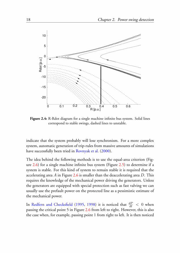
A method that does not rely on a two machine model is the R-Rdot algorithmTaylor et al. (1983); Haner et al. (1986) where the time derivative of the appar-ent resistance versus the apparent resistance is plotted in a diagram. The use ofa time derivative enables some sort of prediction of the type of swing, stable orunstable. In Figure 2.4 we see the R-Rdot diagram for a single machine infinitebus system. For a system such as this we can define a line (here at R = 0.4)that will trip the relay when R-Rdot passes through the line. The basic principlebehind the R-Rdot relay is that the apparent resistance is a measure of the anglebetween the swinging units. Consequently, Rdot is a measure of rotor speedbetween the swinging units. A high speed when the angle is large will then
18 Chapter 2. Power swing detection
0 0.1 0.2 0.3 0.4 0.5 0.6
-20
-15
-10
-5
0
5
10
R [p.u.]
Rd
ot
[p.u
.]
Figure 2.4: R-Rdot diagram for a single machine infinite bus system. Solid linescorrespond to stable swings, dashed lines to unstable.
indicate that the system probably will lose synchronism. For a more complexsystem, automatic generation of trip-rules from massive amounts of simulationshave successfully been tried in Rovnyak et al. (2000).
The idea behind the following methods is to use the equal-area criterion (Fig-ure 2.6) for a single machine infinite bus system (Figure 2.5) to determine if asystem is stable. For this kind of system to remain stable it is required that theaccelerating area A in Figure 2.6 is smaller than the deaccelerating area D. Thisrequires the knowledge of the mechanical power driving the generators. Unlessthe generators are equipped with special protection such as fast valving we canusually use the prefault power on the protected line as a pessimistic estimate ofthe mechanical power.
In Redfern and Checksfield (1995, 1998) it is noticed that dPdt < 0 when
passing the critical point 5 in Figure 2.6 from left to right. However, this is alsothe case when, for example, passing point 1 from right to left. It is then noticed

2.1. Power swing and detection variables 19
Vs Vr
Rs
Figure 2.5: Single machine infinite bus system used in algorithms by Redfern andChecksfield (1995, 1998); Minakawa et al. (1999)
that the reactive power extracted at the receiving end, given by:
Q =Vs Vr
Xcos δ − V 2
r
X(2.2)
is smaller than −V 2r
X for δ ∈ [90, 270]. Since point 5 occurs for load angles
0 45 90 135 180
PMech
51
load angle δ[]
2
3
4
Pow
er
D
A
Figure 2.6: P-δ diagram used for equal-area calculations
greater than 90 then if:
Q ≤ −V 2r
X= Qtrip (2.3)
the machine must be operating at point 5 and not point 1. For machine protec-tion, we consider Vs the internal voltage in the generator and Vr the bus voltage

20 Chapter 2. Power swing detection
where the relay is located. An estimate of Qtrip is then given by:
Qtrip = −Sgen
Xq(2.4)
where Sgen is the rated power of the generator and Xq is the quadrature axissynchronous reactance. The last requirement for being unstable is then thatP ≤ PMech. To summarize, we can conclude that the system will exhibit lossof synchronism if:
P ≤ PMech
Q ≤ Qtrip
dP
dt≤ 0
In Minakawa et al. (1999) a similar approach is used but current is used insteadof reactive power. The requirement on reactive power in the previous algorithm
0 45 90 135 180
0
IP
PMech
Figure 2.7: P and I versus δ
is now replaced with dIdt ≥ 0 to assure that the correct point is identified. Visual
inspection of Figure 2.7 gives that the algorithm can the be summarized to
P ≤ PMech
dI
dt≥ 0
dP
dt≤ 0

2.2. Fault discrimination using circle fitting 21
Both of the mentioned methods are detectors in that they detect when theunstable equilibrium point (5 in Figure 2.6) is passed from left to right. If thepost-fault swing curve is known we can instead predict an out-of-step conditionalready at the last switching instant (3-4 in Figure 2.6). A possible scheme forthis would then be
• During fault
– Obtain the load angle by integrating the frequency difference givenby the actual frequency minus the frequency at the fault inception.
– Calculate the accelerating area (A) by integrating the prefault powerminus the actual electric power.
• Postfault
– Fit a sinusoid to the postfault swing curve. This includes calculatingan additional angle as the estimated load angle is zero at the faultinception.
– Based on the estimated swingcurve calculate the maximum deac-clereating area (D). If D is smaller than A then trip.
In Centeno et al. (1993, 1997) real-time synchronized measurements of thevoltage-phasors at each end of a two machine system is used to estimate the sys-tem parameters. The estimated system is then used to predict the swings and tellif they are stable or not. The method is elegant in that there is no need to supplymodel parameters as they are continuously estimated. However, the equipmentis expensive and also requires communication between the measurement points.
2.2 Fault discrimination using circle fitting
In this section a new method to distinguish a fault from a power swing is presen-ted. The method is based on the phenomenon that the apparent impedanceseen by a relay moves on a circle during a power swing Poage et al. (1943);Clarke (1945). The characteristics of a circle (radius and centre) can then beused to distinguish a fault from a power swing.
22 Chapter 2. Power swing detection
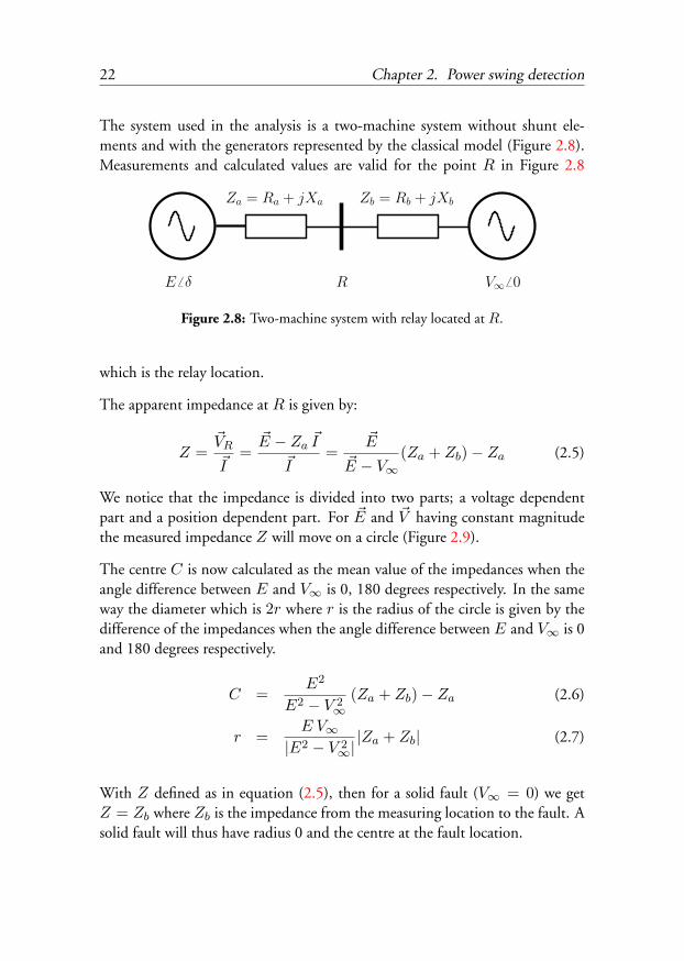
The system used in the analysis is a two-machine system without shunt ele-ments and with the generators represented by the classical model (Figure 2.8).Measurements and calculated values are valid for the point R in Figure 2.8
R
Za = Ra + jXa Zb = Rb + jXb
V∞6 0E 6 δ
Figure 2.8: Two-machine system with relay located at R.
which is the relay location.
The apparent impedance at R is given by:
Z =~VR
~I=
~E − Za~I
~I=
~E
~E − V∞(Za + Zb)− Za (2.5)
We notice that the impedance is divided into two parts; a voltage dependentpart and a position dependent part. For ~E and ~V having constant magnitudethe measured impedance Z will move on a circle (Figure 2.9).
The centre C is now calculated as the mean value of the impedances when theangle difference between E and V∞ is 0, 180 degrees respectively. In the sameway the diameter which is 2r where r is the radius of the circle is given by thedifference of the impedances when the angle difference between E and V∞ is 0and 180 degrees respectively.
C =E2
E2 − V 2∞
(Za + Zb)− Za (2.6)
r =E V∞
|E2 − V 2∞||Za + Zb| (2.7)
With Z defined as in equation (2.5), then for a solid fault (V∞ = 0) we getZ = Zb where Zb is the impedance from the measuring location to the fault. Asolid fault will thus have radius 0 and the centre at the fault location.

2.2. Fault discrimination using circle fitting 23
−1 −0.5 0 0.5 1
0
0.2
0.4
0.6
0.8
1
1.2
1.4
1.6
1.8
2
C
r
X
R
Figure 2.9: Impedance seen by relay.
In the more general case where shunt elements are allowed we can use theABCD parametrization of the circuit,[
Vs
Is
]=[A BC D
] [Vr
Ir
](2.8)
where A,B,C,D are complex constants. Provided that we measure at thesending end then Poage et al. (1943) has derived the following expressions forthe centre and radius:
C =BD 6 β −∆
D2 −(
VrVs
)2 (2.9)
r =
∣∣∣∣∣∣∣B(
VrVs
)D2 −
(VrVs
)2
∣∣∣∣∣∣∣ (2.10)
where B = B 6 β and D = D 6 ∆.
Either the centre or the radius can be used as a fault detector. The radius ispreferred because of the property that it becomes zero when there is a solid fault

24 Chapter 2. Power swing detection
on the line. It is thus easier to find a suitable limit for a fault detector whenusing radius instead of centre.
The results shown above are valid when there is a fault on a line. For a systemwith parallel lines it is also interesting to look at behaviour on the healthy lines.A system with two parallel lines which have a fault on one line can be trans-formed to a single line system by converting the generator and the faulted partof the line to an equivalent two-pole as in Figure 2.10. If the fault occurs such
R
E 6 δ V∞6 0
Zline
Zeq Zssc
Zfault1 Zfault2
R ZlineZeq‖Z
fa
ult
1
Zssc‖Z
fa
ult
2
V ′∞6 θ′E′ 6 δ′
Figure 2.10: Faulted system and equivalent system seen by the relay.
that E′ ≈ V ′∞, then we get a radius that is large or even infinite which in turn
corresponds to a healthy condition of the line, see Figure 2.11. This is actuallycorrect as the monitored line is healthy, the fault is on the parallel line. Whatwe can conclude is that the proposed approach, sometimes will detect a fault ona parallel line as a power swing.
Estimation
The radius and centre can be calculated by fitting a circle to the impedancemeasurements and then identifying the different parts.
A circle in cartesian coordinates is described by:
r2 = (R−R0)2 + (X −X0)2 (2.11)

2.2. Fault discrimination using circle fitting 25
0 0.2 0.4 0.6 0.8 110
−5
100
105
r [p
.u.]
0 0.2 0.4 0.6 0.8 110
−5
100
105
r [p
.u.]
Fault Location
Figure 2.11: Radius (r) as a function of fault distance from the generator (E).The upper graph is for V∞ having a much larger impedance thanin the lower graph. The dashed lines are the radius for unfaultedsystem with one and two lines in operation.
where the centre C = R0 + jX0. With the change of variables:
Z2 = r2 −R20 −X2
0 (2.12)
we get the regression model
R2 + X2 = Z2 + 2RR0 + 2XX0 (2.13)
where we estimate R0, X0, Z2 and then calculates r from equation 2.12
This estimation can for example be done by using a sliding window, a Kalmanfilter or any other kind of recursive least squares method. The recursive versionsshould be equipped with some sort of change detector that restarts the estimatorwhenever there is a large jump in the data.

26 Chapter 2. Power swing detection
When applying a recursive method to equation 2.13, two problems are noticed.
• The estimates drift away during normal operation. This is probably dueto that the measured impedances are located around a short segment ofa circle. The estimator sees this as a circle with centre at the measuredimpedance.
• The convergence at changes is sometimes poor with lots of jumps in theestimated parameters before they settle. This will likely happen whenthere are to few points to make a good estimate. This can be curedif we can provide some extra information about the circle, such as anapproximate location of the centre.
Both of these problems can be solved by restricting the values that the centrecan have.
From equation 2.5 we find that the centre is located on a line. A first approach isthus to restrict the centre to be on a line. This will prevent the drift of the centreand will possibly speed up the convergence too. If, however, we can assumethat the parameters of the line will change considerably, then restricting thecentre to be on a specific line may deteriorate the performance of the estimator.In such a case it might be advantageous to restrict the centre to be within arestricted area of the impedance plane. Two possible area-restrictions are shownin Figure 2.12. The restriction shown to the left in Figure 2.12 is easier toimplement because when the estimate is outside the admissible region, then therestricted estimate is located on the closest border. This can be accomplishedwithout evaluating the loss-function itself. For the restriction to the right inFigure 2.12 we must choose between two lines and the intersection of the lines.This requires evaluation of the loss-function at several different points.
The restricted or constrained estimate can be obtained in the following wayGoodwin and Payne (1977).
A normal least-squares problem
Y = Φθ (2.14)
where θ is the unknown parameter vector, Y is the measurement vector and Φ

2.2. Fault discrimination using circle fitting 27
X
R
X
R
line impedance
Figure 2.12: Possible area-restrictions for the centre.
is the regressor matrix we have the solution
θ = (ΦT Φ)−1ΦT Y (2.15)
We now introduce linear constraints
Lθ = C (2.16)
The minimum variance unbiased estimator θ subject to the constraints Lθ = Cis then given by:
θ = θ − (ΦT Φ)−1LT (L(ΦT Φ)−1LT )−1(Lθ − C) (2.17)
Here, the constraints C, are the boundaries of the admissible area for the centre.
What remains now is to incorporate the constrained estimate into the recursivealgorithms. This is shown for the standard recursive least-squares method andis then applied in the same way on the methods which are suited for detectionof varying parameters.
First we define our regressor, observation and parameter vectors
ϕk =[1 2Rk 2Xk
]Tyk = R2
k + X2k θ =
[Z2 R0 X0
]T

28 Chapter 2. Power swing detection
Next we collect the regressors and measurement up to time k
Φk =
ϕT1...
ϕTk
Yk =
y1...
yk
Introduce the matrix
Pk =
(k∑
i=1
ϕiϕTi
)−1
= (ΦTk Φk)
−1
Finally we can write the update of the estimates as
P−1k = P−1
k−1 + ϕkϕTk (2.18)
θk = θk−1 + Pkϕk(yk − ϕTk θk−1) (2.19)
To constrain the estimates of a recursive least-squares type algorithm we thushave to use equation 2.17 when the estimates are outside the desired area, wherewe substitute (ΦT Φ)−1 with Pk.
A comparison between the constrained and the unconstrained algorithms canbe seen in the lower part of Figure 2.13.
Choice of estimator
Among the vast number of estimators that can be used to solve 2.13 only a fewhave been tried. Their performance will be shortly reviewed.
Least Squares The least squares method applied on a sliding window withfixed length works but the performance is poor for abrupt changes. Theperformance for slow motion of the measured impedance is also poor. Inboth cases this depends on the fixed length of the sliding window. For theabrupt changes we wold like a short window so that we quickly changefrom prefault to postfault data in the window. For slow motion of themeasured impedance however, we would like to use a long window sothat the distance between the endpoints is large. A window that becomes

2.2. Fault discrimination using circle fitting 29
100 150 200 250 300 350
100
150
200
250
300
R [Ω]
X [Ω
]
0 0.2 0.4 0.6 0.8 1 1.2 1.4 1.6 1.8 2
0
200
400
600
800
1000
r [Ω
]
0 0.2 0.4 0.6 0.8 1 1.2 1.4 1.6 1.8 2
0
200
400
600
800
1000
t [s]
R0 [Ω
]
Figure 2.13: (Top),Measured resistance and reactance after a fault is removed(after 0.5s). (Bottom), Estimated radius (top) and real part of centre(bottom). Solid line is unconstrained algorithm and dashed line isthe constrained algorithm.

30 Chapter 2. Power swing detection
small at abrupt changes and then grows with each sample will probablysolve most of these problems. If the solution needs to be constrained theobtained estimates are often “noisy”. The reason for this is that there isno “memory” in the algorithm, at each time a completely new estimateis calculated. Compare this to the recursive estimators where the newestimate is obtained as the old estimate plus a correction,
Recursive Least Squares The behaviour of the recursive least squares estim-ator is better than the normal least squares estimator. Most problematicis when there is lack of excitation, that is when we operate at or close tosteady state. If we use forgetting, then the estimates start to drift aftersome time. It is a well known problem and can be solved by using con-ditional updating. The performance when the estimates are constrainedis better than for the normal least squares algorithm but is still “noisy”.
Kalman Filter The behaviour of the Kalman filter is better than the recursiveleast squares. In particular we can take advantage of that the estimates ofthe centre (resistance and reactance) are correlated. The degree of correl-ation will change with operating and fault conditions. Even if the degreeof correlation is wrong there is a clear improvement in the result whencorrelated process noise is used compared to uncorrelated process noise.The behaviour when the estimates are constrained is much better thanfor the previous algorithms with a smooth estimate when the constraintis encountered.
Directional Forgetting The algorithm in Cao and Schwartz (2000) which isshown in equation 3.38 on page 66 has been used. The algorithm hasbeen somewhat modified so that the choice of updating is not only basedon the norm of the regressor but on the size of the prediction error.The results are comparable to the results obtained with a Kalman filter.The behaviour when the estimates are constrained is also similar with asmooth estimate when the constraint is encountered.
For the reasons described above the Kalman filter and the directional forgettingalgorithms have been the most used estimators in the case studies.

2.2. Fault discrimination using circle fitting 31
Numerical considerations
When the sending and receiving voltage magnitudes are equal, then the centreand the radius as given by (2.6,2.7) approaches infinity. This of course leads tonumerical problems. Furthermore, the impedance itself is large or infinite whena line is disconnected.
Looking for other parametrizations of the problem we find that if using powerinstead of impedance then the measurements are limited. The trajectories are,however, not longer limited to circles but are instead ellipses. Using admittanceinstead of impedance we find that the trajectories are circles and the admit-tance will only be “infinite” for bus-faults. To investigate the behaviour of theadmittance we notice that the admittance is given by
Y =1Z
(2.20)
but (2.20) is also a Mobius transform which has the property that it maps circlesonto circles. Here, straight lines are considered as circles with infinite radius.Impedance “circles” that will be transformed to lines are thus those that passthrough the origin. From (2.5) we get that this is when
Z = 0 →~E
V∞= −Za
Zb(2.21)
that is for any system that has
E
V∞=|Za||Zb|
(2.22)
This is equivalent to the potential at the measuring point being zero when ~Eand V∞ are in phase opposition.
By working with admittance instead of impedance, potential problems whenE ≈ V∞ are circumvented. On the other hand, a new case for potential nu-meric problems has appeared. A major drawback with circle estimation in theadmittance plane is that the technique to restrict the permitted values of thecentre requires linear constraints. Even a simple constraint such as the one tothe left in Figure 2.12 will be translated into an area between two circles. Re-stricting the centre to be on a line through the origin will however still work.

32 Chapter 2. Power swing detection
Estimator resetting
The applied recursive estimators are designed to follow slowly varying paramet-ers. For large changes, however, they might lose track of the parameters. Thecommon way to resolve this is to restart the estimator when an abrupt change inthe parameters is detected. Here, the prediction error is the detection variable.A large prediction error would then indicate that the used model is no longercorrect. Using a fixed value for the resetting showed to be difficult. This can beexplained by referring to Figure 2.15. A larger error can be tolerated for meas-urements that are far from the origin than for measurements close to the origin.One way to solve this is to make the reset limit dependent on the impedanceplus an additional constant that defines the smallest required accuracy. Simu-lations have shown that making the limit 5%-10% of the measured impedancegives a good result.
In Figure 2.15 it can also be noted that the fault occurs at 0.4 s but the imped-ance does not move directly to the new value. Instead a large detour is madewhich depends on how the impedance is calculated. Here, voltages and currentsare evaluated over a whole cycle of the fundamental frequency to get the rmsvalue and phase. The correct value is thus not available until 0.42 s. Trying toestimate a circle on the detour is not of much use so the criteria for resettinghave to be changed.
Several possible change detectors can now be used to solve this problem. TheCUSUM (Cumulated Sum) detector will signal a change when the monitoredvariable, here the prediction error, has had the same sign and been too largeso that the cumulated sum of the prediction errors reaches a specified value.Since the limit on prediction errors were adjustable it is hard to find a limit forthe detector. An alternative approach is to raise an alarm when the predictionerrors have had the same sign and been larger than the limit for a fixed numberof samples. This will result in a delayed resetting. Simplifying this we canchoose to just schedule the resetting of the estimator with a fixed delay whenthe prediction error is sufficiently large. Scheduling of another reset is theninhibited until the reset has taken place. The latter approach is implementedand has worked satisfactory.

2.3. Case studies 33
2.3 Case studies
The studies are performed on a system that consists of a generator connectedto an infinite bus through a double line. At 0.4 s a fault occurs a fourth ofthe line-length away from the generator on one line. The radius is calculatedfrom measurements on the healthy line. The faulted line is cleared at differenttimes producing both stable and unstable swings. The simulations were done in“Power System Blockset” in MATLAB, SIMULINK. Simulation is done in phasequantities.

34 Chapter 2. Power swing detection
Small oscillation
The fault is cleared by opening the faulted line at 0.5 s resulting in a smalloscillation.
0 50 100 150 200 250 300 350 4000
50
100
150
200
250
300
350
400
R [Ω]
X [Ω
]
0 0.5 1 1.5 2 2.5 3 3.5 4 4.5 50
100
200
300
400
500
600
700
r [Ω
]
Figure 2.14: Impedance loci seen from R (top) and estimated radius (bottom).Fault at 0.4 s, fault cleared at 0.5 s. The mark in the upper diagramis at 0.54 s

2.3. Case studies 35
Large oscillation
The fault is cleared by opening the faulted line at 1.2 s resulting in a very largebut stable swing.
−500 −400 −300 −200 −100 0 100 200 300 400 500−100
0
100
200
300
400
500
600
700
800
R [Ω]
X [
Ω]
1.2s0.42s
1.24s 1.22s
0.4s
0 0.5 1 1.5 2 2.5 3 3.5 4 4.5 50
50
100
150
200
250
300
350
400
450
500
r [Ω
]
Figure 2.15: Impedance loci seen from R (top) and estimated radius (bottom).Fault at 0.4 s, fault cleared at 1.2 s.

36 Chapter 2. Power swing detection
Reclosing
The faulted line is opened at 0.7 s reclosed on th the fault again at 1.2 s andfinally opened at 1.5 s.
−500 0 500−200
−100
0
100
200
300
400
500
600
700
800
900
R [Ω]
X [Ω
]
0 1 2 3 4 50
100
200
300
400
500
600
700
r [Ω
]
Figure 2.16: Impedance loci seen from R (top) and estimated radius (bottom).
2.3. Case studies 37
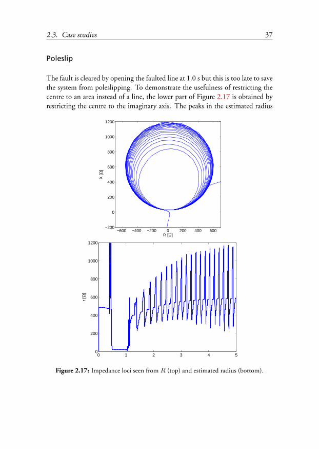
Poleslip
The fault is cleared by opening the faulted line at 1.0 s but this is too late to savethe system from poleslipping. To demonstrate the usefulness of restricting thecentre to an area instead of a line, the lower part of Figure 2.17 is obtained byrestricting the centre to the imaginary axis. The peaks in the estimated radius
−600 −400 −200 0 200 400 600−200
0
200
400
600
800
1000
1200
R [Ω]
X [Ω
]
0 1 2 3 4 50
200
400
600
800
1000
1200
r [Ω
]
Figure 2.17: Impedance loci seen from R (top) and estimated radius (bottom).

38 Chapter 2. Power swing detection
are due the measured impedance not forming perfect circles with the centreon the imaginary axis. Allowing X0, R0 to be in a specified area such as inFigure 2.12 improves the result drastically. as seen in Figure 2.18.
0 1 2 3 4 50
100
200
300
400
500
600
700
r [Ω
]
Figure 2.18: Estimated radius when both R0, X0 are free.
Comments
The simulation results seems a bit strange as there should only be one circleinstead of two. This is probably because the used generator model is not atrue representation of the classical model. Most probably it incorporates bothsynchronous and transient reactances although it claims not to do so.
2.4 Concluding remarks
Power swing detection can often be replaced by fault detection in distance pro-tection of transmission lines. The idea is to detect fault or non-fault instead ofa power swing. This has the advantage that fault detection is faster than swingdetection because power swings are a slow phenomena compared to faults. Inthis context, a power swing is regarded as normal, although undesirable opera-

2.4. Concluding remarks 39
tion. A method suggested in the literature is to use the fault transient as a faultindicator. If the apparent impedance enters the protected zones within a spe-cified time after a transient, then the system is believed to be in a faulted stateand the relays are tripped. Possible problems with this setup is to tune the timerand how to distinguish a fault transient from the disconnection of the fault ordisconnection/reconnection of a line.
A new fault-detection method, based on the physical behaviour of a two ma-chine system is proposed. The method works by finding a new coordinatesystem in which it is easier to distinguish faults from non-faults. The newcoordinate system uses the fact that the apparent impedance seen in a two ma-chine system moves on a circle. The proposed method does not rely on timersor transients and needs virtually no tuning. When evaluated on a number ofcase studies with parallel lines, all faults were detected as faults and all powerswings were detected as non-faults.

40 Chapter 2. Power swing detection

Chapter 3
Damping estimation
In this chapter different methods to determine frequency and damping of electro-mechanical oscillations in a power system will be discussed. There are two ap-proaches to this, (1) ring-down analysis and (2) normal operation analysis. Inring-down analysis, signals measured after a large disturbance are used to cal-culate the eigenvalues of the monitored system. The disturbance can be a lineswitching, fault, probing by HVDC or anything else that have a large impacton the system. These disturbances are typically pulse or step disturbances. Asthe large disturbances occur infrequently it can be assumed that the observedring-down is due to only one disturbance and hence the observed behaviourcan be regarded as a step or pulse response of a system with unknown initialconditions. To cover for the nonlinear dynamics, a high-order linear model isfitted to the observed ring-down. Different methods can be used but the onethat seems to most common in the power systems area is Prony’s method see forexample Hauer et al. (1990); Pierre et al. (1992). A comparison between threedifferent methods has been performed in Sanchez-Gasca and Chow (1999).
In normal operation identification, the system is only excited by ambient data,this was probably first exploited in Pierre et al. (1997). In that paper the electro-mechanical dynamics of the WSCC system was identified from an hour longmeasurement of active power on a major transmission line. Identification fromambient excited systems serves two purposes:
41

42 Chapter 3. Damping estimation
• In a long timescale, the obtained information can be used to calibratemodels. It can also aid in generation planning in that infeasible regionswill be detected.
• In a short timescale, it is possible to track time varying dynamics. Incase an infeasible region is entered operators can be alarmed or specialprotection schemes can be enabled automatically. The tracking capab-ility has been investigated in Hauer et al. (1998) where it was foundthat proper determination of the damping was a major obstacle. Theestimates turned out to have a large standard deviation compared to thefrequency estimates.
Estimation of time varying dynamics often requires the use of recursive al-gorithms. It can be argued that any algorithm that operates on a batch of datacan be used for estimation of varying parameters by performing the estimationon the last N samples. This, however, is often computationally expensive andalso introduce dependency on old data that is not valid after, for example, a linedisconnection.
The rest of this chapter will discuss choice of suitable measurement signals anda review of some methods that can be used to identify t power system dynamics.Attention is paid to the case where the system is excited only by ambient noise.
3.1 Input signals
Determination of frequency and damping of electro-mechanical modes in apower system is an output-only identification problem. Proper determinationof damping from spectral estimates requires, according to Bendat and Piersol(1980), that four conditions are fulfilled: (1) The auto-spectrum of the excita-tion, Gxx(f), must be reasonably uniform over the frequency of the mode; (2)the relative damping ζi must be small; (3) the analysis resolution bandwidth Be
must be much smaller than the half-power point bandwidth Bi of the mode,and (4) the mode must not overlap heavily with neighbouring modes. Theserequirements can formally be expressed as:
1. Gxx(f) ≈ constant for fi − 3Bi ≤ f ≤ fi + 3Bi.

3.1. Input signals 43
2. ζi < 0.05
3. Be < 0.2Bi
4. (fi − fi−1) > 2(Bi + Bi−1)
Where the relative damping ζ for a pair of eigenvalues at σ ± jω is defined as:
ζ =−σ√
σ2 + ω2(3.1)
For power systems, some of these conditions are not always met or are unknownat the time of estimation. Condition 1 is unknown during normal operationand results from Johansson and Martinsson (1986); Ledwich and Palmer (2000)indicate that the excitation has a low-pass characteristic. Condition 2 can beviewed as the wanted result and is thus not an issue. Condition 3 depends onthe method in use and the data available and is not considered here. Finally,condition 4 is also unknown.
It is suggested that cross-spectrum estimates should be preferred over auto-spectrum estimates. Cross-spectral estimates together with the coherence func-tion will then aid in determining if a peak in the spectral estimate is due toa peak in the exciting signal or to a mode in the system. As focus here is ondamping estimation from local measurements, cross-spectrum estimates are notavailable unless cross-spectrum with mixed units are considered.
Choice of measurement signal
Active power on a transmission line is the signal that seems to be the mostcommon in use for determination of electro-mechanical (EM) mode paramet-ers (frequency and damping). From a systems view this choice is sensible in thatan oscillation is due to a power imbalance at the swinging generators. The miss-ing/exceeding power thus have to be transferred to/from the generators on thetransmission lines. From an estimation point of view it means that the meas-ured variable is closely connected to the phenomenon that is to be estimated,which is good. Among the drawbacks are that many estimation techniques re-quire the signal to have a mean value of zero. Furthermore, the mean level ofthe power can make large jumps. Both these inconveniences can be taken care

44 Chapter 3. Damping estimation
of by proper pre-filtering of the signal. Due to the non-linear dynamics of apower system, large oscillations will be accompanied with harmonics, whichmakes estimation more difficult. For power this becomes apparent when theangle between swinging machines approaches and exceeds 90. With the fre-quency range of interest spanning about a decade there is not much that canbe done about this but increasing the model order or changing the estimationsignal.
The angle between swinging machines is a signal that is perhaps even moretightly connected to the oscillation phenomena. Until recently it has, however,been impossible to measure. An angle difference measurement is obviouslynot a local measurement and thus requires a viable communication structure.The properties of angle difference are similar to those of active power. Forlarge oscillations, angle difference is not as nonlinear as active power, therebyreducing the amount of harmonics.
If mode estimation is performed at the distribution level, which could be thecase for damping controllers, then information on transmission line power isunavailable. Signals at this level that contain system wide information are fre-quency and voltage. Voltage share many of the properties of power but theconnection to the swing phenomena is weaker. The influence on voltage causedby electro-mechanical oscillations can be expected to be small because of thevoltage control on the generators. Modern voltage control is typically muchfaster than the electro-mechanical oscillations.
Local frequency share most of the properties with angle difference. An ad-vantage with frequency is that the jumps visible in power, angle difference andvoltage measurements are removed by the integral relation between frequencyand angle. Depending on system, however, frequency measurements might havea substantial low frequency (up to 0.05 Hz) behaviour which is not present inthe other measurements. This comes from the rigid body motion caused byfrequency control.
A closer look at frequency and voltage
Assuming a single machine infinite bus system, what can be expected to be seenin frequency/voltage measurements? For simplicity, only the case with a purely

3.1. Input signals 45
reactive transmission-line and the classical generator model is studied.
Vl 6 δl
a
V∞6 0Vg 6 δg
Figure 3.1: Single machine infinite bus system, where a is the relative distancefrom the infinite bus to the generator.
V∞δl
δg
Vg
Vl a
Figure 3.2: Voltage vectors for the infinite bus system in Figure 3.1.
The angle of the voltage vector at a distance a from the infinite bus is given by:
δl = arctan(
aVg sin(δg)(1− a) V∞ + aVg cos(δg)
)(3.2)
Taking the derivative of this with respect to the angle of the voltage vector atthe generator gives
dδl
dδg=
aV∞Vg cos(δg)(1− a) + a2V 2g
2aV∞Vg cos(δg)(1− a) + (1− a)2V 2∞ + a2V 2
g
(3.3)
which always have a value in [0, 1] (Figure 3.3) for 0 ≤ δg ≤ π/2, with equalityfor a = 0 and a = 1. The quantity dδl
dδgcan be seen as an observation gain,

46 Chapter 3. Damping estimation
that is how much does our observation change when the generator oscillates.An oscillation in this system is thus best observed as close as possible to theswinging generator (a = 1 → dδl
dδg= 1). Assuming a sinusoidal oscillation,
0 0.2 0.4 0.6 0.8 10
0.2
0.4
0.6
0.8
1
a
dδl /d
δ g
Figure 3.3: dδl
dδgas function of a for Vg = V∞ = 1 and δg = 0 (solid), π/4
(dashed) and π/2 (dotted).
the instantaneous voltage somewhere along the line can be described as a phasemodulated signal with amplitude V :
V (t) = V sin(ωt + ∆0 + ∆g sin(ωosct)︸ ︷︷ ︸θ(t)
) (3.4)
Taking the time derivative of the phase angle θ(t) gives the instantaneous fre-quency
dθ
dt= ω + ∆gωosc cos(ωosct) (3.5)
With ω = 100π, ∆g = 1 and ωosc = π, this gives a maximal change infrequency of ±9mHz which corresponds to a change in cycle-time of ±3.5µswhich is less than 1h of the cycle-time of the fundamental.
Performing the same kind of analysis on the measured voltage gives the voltage

3.1. Input signals 47
magnitude
Vl =√
a2V 2g + (1− a)2V 2
∞ + 2a(1− a)V∞Vg cos(δg) (3.6)
and the change in voltage due to generator swing
dVl
dδg=−a(1− a)V∞Vg sin(δg)
Vl(3.7)
This result is however not as easy to interpret as the result for frequency meas-urement. With sensible values on Vg and V∞, the result from equation 3.7will most certainly be small but the result depends heavily on Vg and V∞ asseen in Figure 3.4. When using change in voltage it thus best to look some-
0 0.2 0.4 0.6 0.8 1−0.4
−0.3
−0.2
−0.1
0
a
dVl /d
δ g
Figure 3.4: dVl
dδgas function of a for Vg = V∞ = 1 and δg = π/4 (dashed) and
π/2 (dotted) and for Vg = 1.2, V∞ = 1 and δg = π/4 (solid) andπ/2 (dash-dotted).
where between the swinging parts as the oscillation will be unobservable at theendpoints.
Effects of filtering
Filter design is usually performed with pure oscillations even though the filtersare intended to be used with signals that contain a lot of information that is not

48 Chapter 3. Damping estimation
in the form of sustained oscillations.
It has been very difficult to find anything in the published literature about how afilter distorts the damping of a signal, since normal analysis only give amplitudeand phase information. The damping of a signal is closely related to the peak-width when looking at the signal in the frequency domain. For damped signalsit is thus crucial to know how the peak-width is changed by the filter.
As the EM modes are within a known frequency range we will band-pass fil-ter the signals before performing the mode estimation. Traditional filters suchas Butterworth and Chebyshev tend to be like more or less well-tuned reson-ance circuits. Thus, a filter with a narrow passband may oscillate with almostno damping and by this indicating that the system we look at seems closer toinstability than it really is.
Finite Impulse Response (FIR) filters are filters which output only depends onthe input signal, not on the filtered output. Because of this FIR filters do nothave an oscillatory behaviour. For steep and narrow passbands they often tendto need many samples from the input signal and because of this, the time delayfrom input to output can be substantial (several seconds). Many design tech-niques for FIR filters also give filters with ripple in the passband. This is notlimited to FIR filters; Chebyshev type I filters also have this property Claessonet al. (1990).
EXAMPLE
Consider a band-pass filter with ripple in the passband and a signal comingfrom a system with poor damping (Figure 3.5). The spectrum of the filteredoutput as seen in Figure 3.5 is now distorted by the filter in such a way thatboth the frequency and the damping, determined by the width of the peak, ofthe input signal is wrong.
Looking at the poles and zeros of the filter and the oscillatory system, Figure 3.6,we can also see that there is almost a pole-zero cancellation. This means thatif the damping becomes worse, the signal generated from the oscillatory systemmight be close to or completely cancelled by the filter and thus invisible in theoutput.

3.2. Loads and their behaviour 49
|H(e
iω)|
0 5 10 15 20 250
0.2
0.4
0.6
0.8
1
1.2
f [Hz]
Figure 3.5: Spectrum of input signal (dash-dotted), amplitude function for band-pass filter (solid) and spectrum of the filtered output (solid grey). No-tice that the peek has moved and that the shape has changed so muchthat damping estimated from peak-width is wrong.
Conclusions
As a consequence of the results shown earlier, all filters used in this report have aflat characteristic in the passband. The filters used are mostly first order filters.When a higher roll-off is needed several cascaded first order filters have beenapplied. The cascaded filters do not have to have the same cut–off frequency.
3.2 Loads and their behaviour
Loads in power system are typically represented as a mixture of constant power,constant impedance and constant current sources. In recent years, dynamicmodels such as Karlsson and Hill (1994) have been introduced. Common forall these models are that the power they consume is constant unless somethinghappens with the voltage. In our case, we are interested in the random loadvariations in the timescale of seconds, as these variations make the power systemoscillate during normal operation. In Johansson and Martinsson (1986) it isshown that the random load variations have low-pass characteristics and thatthe standard deviation of the load variation is always less than 2%. The largest

50 Chapter 3. Damping estimation
−1 −0.5 0 0.5 1
−1
−0.8
−0.6
−0.4
−0.2
0
0.2
0.4
0.6
0.8
1
Figure 3.6: Poles of oscillatory system ’x’ and zeros of bandpass-filter ’o’. Itis seen that the pole is difficult to see behind the zero when movingalong the unit circle.
deviation from the mean value that has been observed is less than 5% of themean value itself. These results are based on one hour measurements underseveral different load conditions.
In Johansson and Martinsson (1986) it is also shown that the statistical prop-erties of the load changes with the load/time of day, that is the load is not sta-tionary in a stochastic sense. The consequences of this are hard to tell but thechange in load behaviour is probably smaller than the change in power systemdynamics with changing load and time of day.

3.3. Batch estimation 51
3.3 Batch estimation
When doing batch estimation, a model is fit to a number of consecutive meas-urements. This requires that the data has the same stochastic properties forthe whole measurement period. Power systems are, as discussed earlier, not sta-tionary in the stochastic sense. If, however we limit our data to for exampleone hour, then it is probable that the stochastic properties can be consideredstationary during this hour. This means that we can derive a model for thisspecific hour 1.
Linear prediction error methods
The idea behind prediction error methods is to predict future values of a sampledsignal, y(0), y(1), . . . , y(n), by a linear combination of the previous samples.The simplest and most well-known of this class of systems is the autoregressive(AR) model,
y(n) =p∑
k=1
ak y(n− k) + e(n) (3.8)
where e(n) is white noise.
We would now like to determine the coefficients ak such that the predictionerror
ε(k) = y(k)− y(k|k − 1) (3.9)
is minimized. y(k|k− 1) denotes the predicted output at time k given data upto time k − 1. Minimization of all ε(k) with respect to the parameters ak insome norm
J = minak
m∑i=p+1
||y(i)− y(i|i− 1)|| (3.10)
1An hour is probably too long time during the load increase/decrease during morn-ing/afternoon. In this case we might need to use a shorter time interval.

52 Chapter 3. Damping estimation
gives the characteristic polynomial of the model
A(q) = qp − a1 qp−1 + · · · − ap−1 q − ap (3.11)
Solving 3.11 now gives us the frequency and damping of the identified modes.It should be noted that equation 3.8 also can be used in the backward direction,that is calculating y(n) from y(n + 1), y(n + 2), . . . , y(n + p).
Several different methods exist to solve this problem in an efficient way. Well-known methods are the Yule-Walker and Burg methods (Proakis and Manola-kis, 1988, pp 821-831) which can be efficiently solved via the Levinson-Durbinalgorithm. These methods were originally developed for spectral estimation anduse the auto-covariance of the signal rather than the signal itself. The Levinson-Durbin algorithm however makes these methods useless for this applicationbecause the resulting models will always be stable. The Burg algorithm further-more exhibits spectral line splitting at high signal-to-noise ratios and introducesspurious peaks at high model orders.
If we give up the Levinson-Durbin algorithm we get the unconstrained Burgalgorithm which does not have the above mentioned disadvantages. The pricewe pay is that it is computationally more expensive. Instead of working with theautocovariance the description of this method will follow the lines of Kumaresanand Tufts (1982) where we work directly with the data.
Equation 3.8 can be rewritten into matrix form asy(0) y(1) . . . y(p− 1)y(1) y(2) . . . y(p)
...... . . .
...y(n− p) y(n− p + 1) . . . y(n− 1)
ap
ap−1...
a1
=
y(p)
y(p + 1)...
y(n)
(3.12)
or shorter
Y = Φθ (3.13)
Performing singular-value-decomposition (SVD) on Φ (n− p + 1× p) we get
Φ = UΣV H (3.14)

3.3. Batch estimation 53
where U (n − p + 1 × n − p + 1), V (p × p) are unitary matrices 2 andΣ (n − p + 1 × p) is a diagonal matrix with positive values [σ1, σ2, . . . , σp](assuming n− p + 1 > p) on the diagonal. From this we now get
θ = V Σ+UHY (3.15)
where Σ+ is a diagonal (n×m−p+1) matrix with values [1/σ1, 1/σ2, . . . , 1/σp]on the diagonal. The solution given by this method minimizes equation 3.10in 2-norm.
Model order selection
So far we have only dealt with AR(p) models. Our power system is most cer-tainly not an AR(p) system but can be approximated as such a one if we makethe model large enough. What size to choose is difficult but generally we get abetter fit and a smaller J in equation 3.10 when the model order p is increased.The better fit does not imply that we get a more accurate model with respectto the physical system. Most likely we will get what is called overfitting, thatis we also model the noise in the system. Methods such as Akaikes informa-tion criterion (AIC) Akaike (1974) and Rissanens minimum description length(MDL) Rissanen (1978) are methods to help us choose a model order that isnot too large. Still, the models given by one of these criteria will contain a lotof unwanted information. The problem now becomes to find the interestinginformation in the model.
Using the method in equation 3.15 it is often possible to see a jump in thesingular-values (σk), Figure 3.8. This jump can indicate that this is where theuseful information ends, with the remaining singular values corresponding tonoise/overfitting. By setting the singular values after the jump to zero we em-phasize what we think is the important dynamics Kumaresan and Tufts (1982).However, doing this introduces radial bias, which in the discrete frequency do-main corresponds to bias in the real part in the continuous frequency domain,that is, bias in the estimated damping. This bias is smaller the larger the modelis. It can also be compensated for by manipulating the remaining singular val-ues. This method was also suggested in Kumaresan and Tufts (1982) but un-
2A unitary matrix (U) has the property that UH = U−1 and where H denotes complexconjugate and transposition.

54 Chapter 3. Damping estimation
fortunately the instructions are not very clear so this special bias compensationhas not been very successful. In Rao (1988) it is shown that the sensitivity ofthe roots of the prediction polynomial with respect to the filter coefficients de-creases with increasing filter-length. This is only true when the signals are puresinusoids and is of course only valid for the roots belonging to the sinusoids.
The drawback with a model of very high order is that finding the roots of alarge polynomial is numerically difficult.
EXAMPLE
Consider the signal (see Figure 3.7)
y = e−0.01t sin(πt) + e0.0012t cos(1.3πt) + 0.5 e(t)
for t ∈ [0, 100], where e(t) is zero mean Gaussian noise with standard de-viation 1. Bandpass filtering the signal with a fourth order filter and tryingdifferent model orders, AIC and MDL gives us the model orders 198 and 35.Using equation 3.15 with a model order of 200 we get the singular values in
20 25 30 35 40−2
−1.5
−1
−0.5
0
0.5
1
1.5
2
t [s]
Figure 3.7: Signal without noise (solid) and bandpass-filtered noisy signal(dashed).
Figure 3.8. Clearly there is a jump between the fourth and fifth singular value,indicating that there are four interesting poles. In Figure 3.9 the results areshown for models of order 4, 200 and 200 where σ5, . . . , σ200 are set to zero.The fourth order model is obviously poor as there is only one pole(pair) in the
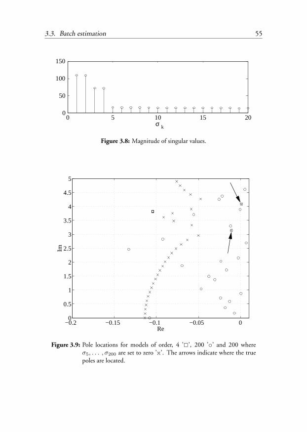
3.3. Batch estimation 55
0 5 10 15 200
50
100
150
σ k
Figure 3.8: Magnitude of singular values.
−0.2 −0.15 −0.1 −0.05 00
0.5
1
1.5
2
2.5
3
3.5
4
4.5
5
Re
Im
Figure 3.9: Pole locations for models of order, 4 ’2’, 200 ’o’ and 200 whereσ5, . . . , σ200 are set to zero ’x’. The arrows indicate where the truepoles are located.

56 Chapter 3. Damping estimation
region, with the other polepair having a large negative real value. The modelof order 200 has poles in the correct locations but also a lot of other polesthat correspond to noise/overfitting. How to find the true poles among theother ones is non-trivial. For the model of order 200 with 4 “dominant”poleswe can see that there are poles at the correct locations and that the rest of thepoles are separated from these four poles, making it easier to find the interestingdynamics. The “dominant” poles for this model are −0.01105 ± i3.1429 and0.001195±i4.0842 which are very close to the correct values−0.01±i3.1415and 0.0012± i4.0841
Other parametrisations
The identification has been performed using the shift operator q, which shiftsdiscrete-time data one step forward. This is just one choice of operator. An-other common operator is the δ operator Middleton and Goodwin (1990).Higher order operators such as the Kautz operator Wahlberg (1991); Kautz(1951) might sometimes be better.
Damping estimation from spectral estimates
Note: The angular frequency (ω) used in this section is the discrete time angu-lar frequency, that is ω = ωc/ωs where subscript c indicates continuous timefrequency and subscript s denotes sampling frequency. In order for the Nyqvistsampling theorem to hold, it must be assured that ωc < 2 ωs.
An alternative to the time domain methods is to determine frequency anddamping from spectral estimates. Provided that the conditions on page 42 arefulfilled, the relative damping can be estimated as:
ζi =Bi
2fi(3.16)
Calculating the absolute damping σ from 3.1 requires the knowledge of ωwhich is different from the peak frequency value. For low damping, the dif-ference is small and the frequency peak value can be used instead of ω.
The spectral estimate can be computed in a number of ways. It should be noted

3.3. Batch estimation 57
that the polynomial identified in the prediction error methods (equation 3.11)can be used to compute the power spectrum as
PLP (ω) =Pe
|A(ejω)|2(3.17)
where Pe is the variance of the prediction error and subscript LP is used todenote linear prediction error method. This approach can be useful for highorder models where it is computationally expensive to find the roots with highaccuracy. The interpretation of the poles or pattern of poles might also be easierto do in the frequency plane.
Fourier transforms
The fast way to compute a spectral estimate is to use the Fast-Fourier-Transformwhich is a special version of the Discrete-Fourier-Transform. Direct usageof these transforms produce, however, poor result on data typical for power-systems. The poor behaviour is probably due to the signals not containing puresinusoids but rather damped sinusoids with varying phase. The estimates aredrastically improved when data is windowed and several estimates are averaged,that is by using Welch’s method. Still, choice of segment length, number ofsegments, window and size of window is an elaborate work.
Capon
The Capon spectral estimator is an estimator that provides a minimum vari-ance unbiased estimate of the spectral components in a signal. It is known thatthe linear prediction (LP) method exhibits sharp peaks, thus having high spec-tral resolution. The spectral envelope is however often poorly modelled whichhas been noticed in, among other fields, speech processing see Murthi and Rao(2000) for a discussion about this. The Capon method, which is a minimumvariance (MV) method, produces a better estimate of the envelope and mightthus be a suitable candidate for a spectral estimator that is usable for damp-ing estimation where the shape of the envelope is important. The theoreticalfoundations of the method can be found in Lacoss (1971) and are not discussedhere.

58 Chapter 3. Damping estimation
The M th order Capon spectral estimate is given by:
P(M)MV (ω) =
1vH(ω)R−1
M+1v(ω)(3.18)
where v(ω) = [1, ejω, ej2ω, . . . , ejMω]T and where RM+1 is the (M + 1)×(M + 1) Toeplitz autocorrelation matrix of the input signal. The autocorrela-tion ryy of a signal y(k) can be estimated by:
ryy(k) =
1N
∑N−kl=1 y(l) y(l + k) k = 0, . . . , N − 1
r(−k) k = −N + 1, . . . ,−10 |k| ≥ N
(3.19)
Alternatively, the spectrum can be parametrically written as
P(M)MV (ω) =
1∑Mk=−M µ(k)e−jωk
=1
|B(ejωk)|2(3.20)
The parameters µ(k) and the spectrum in general can be obtained from the LPcoefficients ak (3.11) and prediction error variance Pe.
µ(k) =
1Pe
∑M−kl=0 (M + 1− k − 2l)ala
∗l+k for k = 0, . . . , M
µ(−k) for k = −M, . . . ,−1(3.21)
Multiple window methods
A multiple window method for spectrum estimation is a method which usesseveral orthogonal windows to estimate the spectrum. The idea behind thisThomson (1982) is that if we have some prior knowledge about what the spec-trum looks like, we can the get a better estimate of that part of the spectrumHansson and Salomonsson (1997). The main problem with this method fordamping estimation is that a spectral estimate does not tell if the input sig-nal is stable or unstable. This method is thus not capable of providing all theinformation we need.

3.3. Batch estimation 59
Chirp z-transform
The idea behind using the chirp z-transform (CZT) is to modify the discreteFourier transform (DFT) to look for growing/decaying oscillations instead ofpure sinusoids. A plot of the DFT of three different test signals is shown inFigure 3.10. It can here be seen that the spectral estimate of the signal becomesflatter the quicker the signal grows.
10−2
10−1
100
101
100
f [Hz]
|Y(ω
)|
DFT
Figure 3.10: DFT of e0.001t sin(πt) (solid), e0.01t sin(πt) (dashed) ande0.1t sin(πt) (dotted).
The DFT of a time signal y(0), y(1), . . . , y(N − 1) is given by:
Y (ωk) =N−1∑n=0
y(n)e−jωk n (3.22)
ωk = 2πk/N (3.23)
with 0 ≤ k < N . We notice that the factor e−jωk n is a point that is locatedon the unit circle, which is where poles to a system with undamped oscillationswill appear. If we now modify this factor so that we get points on a circle withradius r0 we get a transform that is well suited to detect systems that have polesat a distance r0 from the origin.
Y (ωk) =N−1∑n=0
y(n) r0 e−jωk n (3.24)

60 Chapter 3. Damping estimation
By varying r0 we can now search for signals with different damping (Figure 3.11).This is a special case of the CZT; in the full CZT we allow r = r0 rn
δ , where rδ
is a complex constant.
r0
-1 0 1
1
0
-1
Figure 3.11: Search region for the CZT.
Given that a number of CZTs are performed there are two ways to determinethe damping. The first one is to look at the phase of the signal, which wassuggested in Bounou et al. (1992). When r0 is changed, it can happen that apole that was previously inside the circle moves to being outside of the circle.This will show up in the phase as a phase jump of 360 degrees. In the lowerpart of Figure 3.12 it can be seen that there is a phase shift of 180 degrees at0.5 Hz for three of the CZTs, with the fourth one having a phase shift of minus180 degrees. This indicates that the true damping is somewhere in the intervalbetween the dotted line and the dash-dotted line, that is r0 ∈ [1.0002, 1.0004].When the signal is noisy this method cease to work because noise in the inputsignal will show up as phase noise in the CZT, which makes it impossible to seeany difference between phase jumps caused by noise or by the real signal.
The second method is to look at the width of the peak at the resonance fre-

3.3. Batch estimation 61
10−2
10−1
100
101
100
|Y(ω
)|CZT
10−2
10−1
100
101
−200
0
200
400
f [Hz]
arg(
Y(ω
))
Figure 3.12: CZT for e0.01t sin(πt) with r0 0.9998 (solid), 1 (dashed), 1.0002(dotted) and 1.0004 (dash-dotted). r0 corresponding to e0.01t is inthis case 1.00020002
quency. This method is much more robust to noise (see Figure 3.13) but prob-lems arise when there are several peaks in the spectra. Now each peak has tobe analysed separately, which needs segmentation of the spectra into interestingparts and then individual normalization for each peak.
The main drawback with this method is that when the studied system has adamped oscillation that is excited several times during the measurement period,the CZT does not recognize this as a damped oscillation. This is correct, be-cause there are several damped oscillations. It now becomes difficult to determ-ine r0 and r0 is usually found at the upper bound. The chance of false alarm isthus not negligible, which makes this method difficult to use for identificationduring normal operation. This drawback might be compensated for by using ashorter measurement period but this also affects the spectral resolution. If theoscillation frequency is known it is possible to get better resolution around thatfrequency but if this compensates fully for the shorter measurement time is hard

62 Chapter 3. Damping estimation
0
0.4
20
0.45 0.5
40 60
0.55 0.6
80 100
10−2
−20
−15
−10
−5
0
5
10−1
10
15
20
100
f [Hz]
|Y(ω
k)|
t [s]
Figure 3.13: Noisy data and true signal (top), CZTs for noisy data (bottom). r0
0.9998 (solid), 1 (dashed), 1.0002 (dash-dot-dotted) and 1.0004(dash-dotted). The true value of r0 is 1.00020002.
to tell.
Sliding window
The idea of calculating the Fourier transform of a window that slides over asignal and then determine the damping from the different spectral estimateswas first presented in Lee and Poon (1988). It has since been modified to bettercope with multi-mode systems in Lee and Poon (1990); O’Shea (2000, 2002).
3.4. Recursive identification 63
For a single mode system it can be described as:
y(k) = A e(jωc+σ)k + e(k) (3.25)
with e being white Gaussian noise. Assuming rectangular observation windowsthe first window is applied from k = 0 to k = Tw, and the second from k = Tg
to k = Tg + Tw, the estimate of the damping is
σ =1Tg
logFTg(ωc)F0(ωc)
(3.26)
For same reasons as for the chirp-z transform this method requires clean ring-down signals to work.
3.4 Recursive identification
Recursive identification is useful when we want to use the estimated mode-parameters for control or alarm. Doing recursive estimation means that thecomplete model is computed/updated at each sampling interval, which meansthat it is possible to track varying parameters. This implies that the model orderis in some way dependent on the sampling interval as there now is a time limiton each update. Recursive identification techniques furthermore require thatthe parameters in the model vary much slower than the dynamics of the systembeing identified. If this is not the case it becomes impossible to distinguishbetween system dynamics and parameter dynamics. Slower does not mean thatit is impossible to have jumps in the parameters. A line switching for examplewill cause a jump in the parameters but the parameters will then stay at the newvalue until another event occurs. The recursive identification algorithm willnot be able to track the change in parameters instantaneously, it will take sometime depending on the choice of algorithm and tuning parameters. But as longthe time between events is long enough, the algorithm will adjust to the newoperating conditions.
Recursive least squares
The recursive least-squares method solves the same problem as equation 3.10when using the 2-norm. In the case where the parameters (θ) are time-varying
64 Chapter 3. Damping estimation
there is the problem that all information about the past is saved although it maybe increasingly irrelevant. To be able to track varying parameters better, forget-ting is introduced, that is less attention is paid to old data. An alternative is torestart the estimator if for example some change detection algorithm alarms.
The recursive least squares method can be derived in the following way. Firstdefine regressors and parameter estimate:
ϕk =[y(k − p) y(k − p + 1) . . . y(k − 1)
]Tyk = y(k) θ =
[ap ap−1 . . . a1
]Tat time k the data is organised as
Φk =
ϕT1...
ϕTk
Yk =
y1...
yk
which is equivalent to equations (3.12, 3.13). The solution to equation 3.10 attime k can then be written as:
θk = (ΦTk Φk)−1ΦT
k Yk
Introduce
Pk = (ΦTk Φk)−1 =
(k∑
i=1
ϕiϕTi
)−1
(3.27)
after some manipulation the solution can now be expressed as
P−1k = P−1
k−1 + ϕkϕTk (3.28)
θk = θk−1 + Pkϕk(yk − ϕTk θk−1) (3.29)
This formulae is not usually used because of requirement to calculate the inverseof Pk in each iteration. Instead equation 3.28 is rewritten using the matrixinversion lemma so that Pk is updated instead of P−1
k

3.4. Recursive identification 65
Modifying the loss-function (equation 3.10) to forget old samples it now be-comes
J(k) =k∑
i=1
λk−i(y(i)− y(i|i− 1))2 (3.30)
where y(i|i − 1) = ϕTk θk and λ ∈ [0, 1] is our forgetting factor. Performing
the same steps as above the algorithm can now be written as:
εk = yk − ϕTk θk (3.31)
θk = θk−1 + Pkϕkεk (3.32)
Pk =1λ
(Pk−1 −
Pk−1ϕkϕTk Pk−1
λ + ϕTk Pk−1ϕk
)(3.33)
where again θk is the parameter estimates at time k and ϕTk is [y(k− p), y(k−
p + 1), . . . , y(k − 1)] for a model of order p. P(0) is an initial estimate ofthe covariance of the parameters θ. It is commonly chosen as a diagonal matrixwith large positive values on the diagonal. K(k) is a time-varying gain vector.Basic theory of recursive identification can be found in Ljung and Soderstrom(1983).
Directional forgetting methods
Estimator windup is a common phenomenon in recursive identification withforgetting. The new information arriving does not update the parameter es-timates because the prediction error is small. At the same time old informa-tion is constantly forgotten although this information is still valid. After sometime everything about the past is forgotten and the output from the estimatoris highly unreliable even if the prediction error is small. There are several al-ternatives to circumvent this problem. One is to stop the updating when nonew usable information is collected. This requires us to in some way specify acriterion for when the data is usable or not which is non-trivial. Another altern-ative is to only forget old information in the same direction as the new data iscollected; this is called directional forgetting.
Two different methods for directional forgetting have been tried, one from Caoand Schwartz (2000) and one from Parkum (1992). Note: due to the more

66 Chapter 3. Damping estimation
complicated update of the P matrix in these methods, the notation is expressedin pseudo-code which is indicated by the use of the assignment (:=) operatorrather than the equivalence (=) operator. The order in which the calculationsare performed is therefore most important.
The algorithm from Parkum (1992) is expressed as:
K := Pϕk
[I + ϕT
k Pϕk
]−1(3.34)
θ := θ + K(yk − ϕT
k θ)
(3.35)
P :=α1 − α0
α1P + α0I (3.36)
P :=(I −KϕT
k
)P (3.37)
where 0 < α0 < α1 < ∞, which limits the eigenvalues of P between α0 andα1. The upper limit prevents estimator windup and the lower limit guaranteesthat the estimator is always alert to some extent.
The algorithm from Cao and Schwartz (2000) has only one parameter, λ ∈[0, 1] which is the forgetting factor.
P :=
P if |ϕk| < ε
P + 1−λλ
ϕkϕTk
ϕTk P−1ϕk
otherwise(3.38)
(3.39)
P := P−Pϕkϕ
Tk P
1 + ϕTk Pϕk
(3.40)
θ := θ + Pϕk
(yk − ϕT
k θ)
(3.41)
This algorithm also has the property that it works as a least-squares estimatorwithout forgetting when |ϕk| < ε.
Extended Kalman filter
The models described in the previous sections have all been linear in their para-meters. This facilitates the construction of the estimator but to find the modesof the model we have to find the roots of a polynomial. Furthermore, it is

3.4. Recursive identification 67
difficult to incorporate prior knowledge about modes into this kind of modelbecause the information will be spread out on all coefficients in the polyno-mial in a nontrivial way. If we want to identify the actual mode parameters wehave to use a non-linear estimator. The most well-known non-linear estimatoris probably the Extended Kalman filter (EKF). The EKF has been successfullyused for estimation of sinusoids in noise Scala et al. (1996); Scala and Bitmead(1996); Nishiyama (1997) some of these ideas have been used for determinationof frequency and voltage-amplitude in a power system Dash et al. (2000).
It is known that the EKF can have poor convergence properties. The conver-gence properties can be very dependent on the parametrisation of the model.For systems that are highly nonlinear there seems to be some interesting resultsin Julier (1997). In this method the Jacobian of the system is not needed. In-stead noise is processed through the system model to find out the distributionone step ahead.
Because of these factors a number of different models were tried. Describingeither the system as an AR(p) model or the output as a sum of exponen-tially growing/decaying sinusoids. As there exist several implementations ofEKFs with different properties Chui and Chen (1999), a number of differentalgorithms were tested. Unfortunately the achieved results were disappoint-ing. On synthetic data the methods work well but are still very sensitive tounmodelled dynamics. On measured data, however, the methods have failedcompletely. This is not necessarily due to the methods, it might be a poor para-metrisation of the model. Because no usable results have been achieved withEKFs, no models are presented here.
Recursive spectral estimates
As pointed out earlier it might sometimes be easier to get an understandingof the system under identification by looking at a spectral estimate rather thaneigenvalues. It is worth to notice that Pk as defined in equation 3.27 is actuallyan estimate of R−1 used in the Capon method (equation 3.18). This enablesus to easily track the spectral estimate over time.
PMV (ω) =1
vH(ω)Pkv(ω)(3.42)

68 Chapter 3. Damping estimation
If more detailed information is needed it is then possible to solve for the eigen-values. It should be noted that using forgetting in the updates of Pk as in (3.31)makes Pk a biased estimate of R−1. Using the directional forgetting methodsthe interpretation of Pk becomes even more difficult as now only parts of Pk
are updated. Tests have, however, indicated that the spectral estimates obtainedwith these update techniques work.
3.5 Conclusions
A number of different methods for estimation of eigenvalues of a dynamic sys-tem have been investigated. The CZT and FFT sliding window method areunsuitable when working with direct analysis of ambient measurements. Usedon derived quantities, such as the auto-covariance of the data they should beusable. This has, however, not been investigated.
The envelope of a spectral estimate is the key variable when determining thedamping from spectral estimates. Many methods developed for spectral estima-tion focus on the spectral resolution, giving sharp peaks for frequencies presentin the signal. While relevant in many cases it is a major drawback in damp-ing estimation. Among the studied methods, the Capon method often gives asmooth estimate which seems usable for determination of the damping. If usedto track time varying dynamics all spectral estimators have the drawback thatthey are unable to distinguish decaying signals from increasing signals. For sig-nals that are close to pure sinusoids they need to be complemented with anotherdetection mechanism to tell if the system is stable or not.
The LP methods works well in many cases but it can be observed that increasingthe model order move the poles closer to the imaginary axis. One way to avoidhigh model order can be to use another system model. In many cases a loworder ARMA(p, q) model
y(k) = a1y(k − 1) + . . . + apy(k − p) + c0e(k) + . . . + cqe(k − q)
performs much better than a high order AR(p) model. The solution to theARMA model is, however, much more complicated than the solution to theAR model. When using ARMA models on test signals the difference in per-formance compared to AR models was small. This, however, need not be the

3.5. Conclusions 69
case for all systems. Depending on system the more expensive use of ARMAmodels might be justified.
The EKF seems interesting and should probably be studied in more detail. Inparticular it could be beneficial to combine a low order EKF together witha high resolution spectral estimation algorithm. The spectral estimator wouldthen feed the EKF with the imaginary parts of the eigenvalues hopefully makingit easier to determine the damping of of a few selected poles.
Presentation of system damping to an operator is an elaborate task. For linearsystems it can be expressed either as eigenvalues or by a spectrum. It seems thata spectrum is easier to interpret for an operator than the location of eigenvalues.This is especially true for high order models.

70 Chapter 3. Damping estimation

Chapter 4
Damping estimation – Casestudies
In this chapter the algorithms from the previous chapter are tested on four dif-ferent cases. One case is a simulation where the power system becomes unstableafter increasing the transfer on a line. Three cases are based on measurements.Two of these cases represent the NORDEL system which is represented in nor-mal operation and operation with a weakened connection between Sweden andZealand (Denmark). The last case is the event on August 10, 1996 in theWSCC system described on page 2 in the introduction.
Wall-outlet measurements of voltage and frequency were performed at thetechnical university of Denmark in Copenhagen. Despite the small vari-ations in frequency it was possible to identify two modes; one at 0.3 Hzand the other one at 0.5 Hz. The damping was so high that it could notbe determined to more than satisfactory.
A simulation of the NORDEL power system was performed in the ARISTOsimulator. Transfer on a critical line was increased until the system be-came unstable. The unstable mode was identified from different “meas-urements”. Using a recursive estimator with a low order model it waspossible to automatically detect instability before an operator could havedone it.
71

72 Chapter 4. Damping estimation – Case studies
Phasor measurement units were located in a substation close to a large gener-ator in Zealand and in the substation in Sweden where the tie-lines toZealand originate. Upon disconnection of the two 400kV lines betweenSweden and Zealand (leaving only two 130kV lines for the interconnec-tion) an oscillation with a frequency of 0.5 Hz was visible. The dampingof this oscillation was determined within 3 s using a low order recursivealgorithm.
The WSCC system was highly stressed on the afternoon of August 10, 1996.Due to a number of events the system approached small signal instability,which eventually was reached, resulting in separation of the network intofour islands. It will be shown that usage of the described methods wouldhave detected low damping at least 5 min before the separation.
4.1 Wall outlet
Voltage (rms) and frequency were measured in a 230V wall-outlet at the Tech-nical University of Denmark (DTU). There are three measurement series: Thefirst one consists of 10 minutes long measurements from each hour starting atlunch and continuing until midnight. The second one is an entire day (24 h)with small gaps at each hour, needed to save data to disk. The third measure-ment series is a one hour long measurement with each sample time-stamped,with the time coming from a GPS clock. The measurement equipment givesone sample per period of the measured frequency, thus giving a sequence witha varying sampling rate. Analysis was performed on raw data and on data thathad been interpolated into fixed sampling rate but no significant differenceswere observed. Based on this, all subsequent analysis were performed assumingconstant sampling rate. This is an adequate assumption considering that thevariation in sampling frequency is less than 1h of the fundamental.
A number of measurement series were discarded because of large peaks in thefrequency and voltage measurements. These peaks are due to a laser printerconnected to the same outlet as the measurement equipment (Figure 4.1).
Looking closer at frequency (Figure 4.2) and remembering the results fromequation 3.5 we notice that it is probably going to be quite difficult to es-timate the damping from these measurements. In order to get any result, data
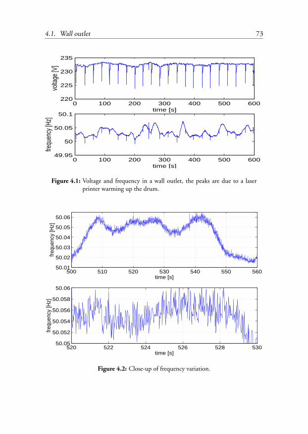
4.1. Wall outlet 73
0 100 200 300 400 500 600220
225
230
235vo
ltage
[V]
time [s]
0 100 200 300 400 500 60049.95
50
50.05
50.1
frequ
ency
[Hz]
time [s]
Figure 4.1: Voltage and frequency in a wall outlet, the peaks are due to a laserprinter warming up the drum.
500 510 520 530 540 550 56050.01
50.02
50.03
50.04
50.05
50.06
time [s]
frequ
ency
[Hz]
520 522 524 526 528 53050.05
50.052
50.054
50.056
50.058
50.06
time [s]
frequ
ency
[Hz]
Figure 4.2: Close-up of frequency variation.
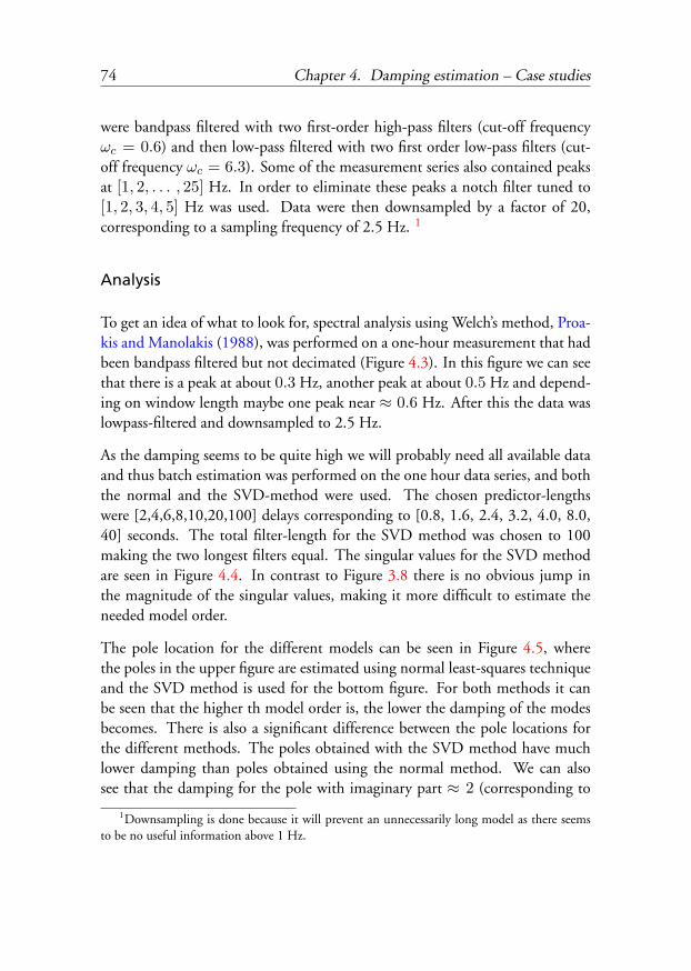
74 Chapter 4. Damping estimation – Case studies
were bandpass filtered with two first-order high-pass filters (cut-off frequencyωc = 0.6) and then low-pass filtered with two first order low-pass filters (cut-off frequency ωc = 6.3). Some of the measurement series also contained peaksat [1, 2, . . . , 25] Hz. In order to eliminate these peaks a notch filter tuned to[1, 2, 3, 4, 5] Hz was used. Data were then downsampled by a factor of 20,corresponding to a sampling frequency of 2.5 Hz. 1
Analysis
To get an idea of what to look for, spectral analysis using Welch’s method, Proa-kis and Manolakis (1988), was performed on a one-hour measurement that hadbeen bandpass filtered but not decimated (Figure 4.3). In this figure we can seethat there is a peak at about 0.3 Hz, another peak at about 0.5 Hz and depend-ing on window length maybe one peak near ≈ 0.6 Hz. After this the data waslowpass-filtered and downsampled to 2.5 Hz.
As the damping seems to be quite high we will probably need all available dataand thus batch estimation was performed on the one hour data series, and boththe normal and the SVD-method were used. The chosen predictor-lengthswere [2,4,6,8,10,20,100] delays corresponding to [0.8, 1.6, 2.4, 3.2, 4.0, 8.0,40] seconds. The total filter-length for the SVD method was chosen to 100making the two longest filters equal. The singular values for the SVD methodare seen in Figure 4.4. In contrast to Figure 3.8 there is no obvious jump inthe magnitude of the singular values, making it more difficult to estimate theneeded model order.
The pole location for the different models can be seen in Figure 4.5, wherethe poles in the upper figure are estimated using normal least-squares techniqueand the SVD method is used for the bottom figure. For both methods it canbe seen that the higher th model order is, the lower the damping of the modesbecomes. There is also a significant difference between the pole locations forthe different methods. The poles obtained with the SVD method have muchlower damping than poles obtained using the normal method. We can alsosee that the damping for the pole with imaginary part ≈ 2 (corresponding to
1Downsampling is done because it will prevent an unnecessarily long model as there seemsto be no useful information above 1 Hz.

4.1. Wall outlet 75
10−2
10−1
100
101
10−4
10−2
100
f [Hz]
10−1
100
10−1
100
f [Hz]
Figure 4.3: Spectral estimate of line-frequency 2001-02-21 (top) and detailsof upper figure (bottom). Data is bandpass filtered, spectrum isestimated with Welch’s method, sampling frequency 50 Hz, FFTlength 16384, Hanning window with length 8192 (solid) and 4096(dashed).
0.3 Hz) changes its location drastically for the normal algorithm with the realpart varying between -1.3 (second order system but imaginary part wrong) upto -0.05 for 100th order system. For the SVD method the change in real partfor this mode is not that large, -0.06 up to -0.045, but as mentioned earlier thedifference between pole location for the two methods is large.
Choosing the appropriate method and model order from the pole location is notobvious. One way to compare different models is to calculate their spectra andcompare with the estimated spectrum in Figure 4.3 which is done in Figures 4.6

76 Chapter 4. Damping estimation – Case studies
0 20 40 60 80 1000
0.02
0.04
0.06
0.08
0.1
k
σ k
Figure 4.4: Singular values (σk) for a 100th order model, notice that there is nosharp jump like in Figure 3.8.
and 4.7. We can now see quite a large difference between the model spectrumfor the low order model and the estimated spectrum. The difference decreaseswith increasing model order and is quite small at 0.3 Hz for the 100th ordermodel (Figure 4.7)
Another way to compare models is to look at the prediction error, or even easier,at the auto-covariance function of the prediction error. If the predictor is good,the prediction errors should be white noise. In Figure 4.8 we can see that the20th order model indeed gives a white prediction error whereas a 20th orderSVD model still have some dependency between the prediction errors. For thesecond order model we can again see that the normal method performs betterthan the SVD method even though the estimated frequency (Figure 4.6 top) isnot correct!
Results
Various model orders and structures have been tried on a one hour measurementseries. Sufficient model order seems to be about 20. The damping for the mode

4.1. Wall outlet 77
−1.5 −1 −0.5 00
0.5
1
1.5
2
2.5
3
3.5
4
4.5
5
Re
Im 2 4 6 8 10 20 100
−0.2 −0.15 −0.1 −0.05 00
0.5
1
1.5
2
2.5
3
3.5
4
4.5
5
Re
Im
2
4
6
8
10
20
100
Figure 4.5: Poles from normal prediction error method (top) and poles from SVDmethod with predictor length 100. Notice the different scales for thereal axes. The 100th order model ’+’ are equal in both figures. Usingthe SVD method the peaks are easier to find from pole locations. Thedamping, however, is to low to be realistic. For both methods it canbe observed that increasing the model order will move the poles closerto the imaginary axis.

78 Chapter 4. Damping estimation – Case studies
10−1
100
10−1
100
f [Hz]
10−1
100
10−1
100
f [Hz]
Figure 4.6: Spectral estimates obtained with Welch’s method of line-frequency(dashed-dotted) and spectrum for second order model (dashed) and100th order model (solid) with 2 dominant poles (top). Spectral es-timates of line-frequency (dashed-dotted) and spectrum for 20th or-der model (dashed) and 100th order model (solid) with 20 dominantpoles (bottom).

4.1. Wall outlet 79
10−1
100
10−1
100
f [Hz]
Figure 4.7: Spectral estimate of line-frequency obtained with Welch’s method(solid) and spectrum from 100 order model (dashed).
at 0.3 Hz is approximately in the interval -0.18 to -0.12 which is sufficientlyhigh. The modes at higher frequencies have even higher damping and are thusnot interesting. The uncertainty in the damping for these modes is also toolarge.
Conclusions
Prediction error methods are good at what they are constructed for, predictingthe next value. For the used data they are not very good at predicting any-thing more than the next sample. Using the same model for predicting M stepsahead results in large prediction errors. This is perhaps more due to the datahaving too large damping than to the method itself. Estimating an M-step pre-dictor (Ledwich and Palmer (2000)) instead of a one step predictor does not

80 Chapter 4. Damping estimation – Case studies
0 5 10 15 20−1
0
1
2x 10
−7
t [s]
r(t)
0 5 10 15 20−1
0
1
2
3x 10
−7
t [s]
r(t)
Figure 4.8: Covariance of the prediction-error for 20th order models (top) andsecond order models (bottom). Dashed lines are from normal pre-diction error methods, solid lines from SVD method with predictorlength 100.
improve the results. For the estimated models it is hard (impossible) to drawany conclusions about the dynamics of the actual system by looking at the rootsof the models. Two models that make almost identical prediction errors canhave vastly different roots. Again this is probably due to the data having a lowsignal-to-noise ratio.
The following behaviour has been observed :
• The higher order of the model, the lower is the damping of all the poles.Whether this is true or if it depends on the fact that the roots of a highorder polynomial have to be found is unknown. But it is known that itis difficult to get high accuracy for roots of high order polynomials.
4.2. Simulated data from Aristo 81
• A short measurement series seems to give models with lower damping.
• A model that is estimated using only a few singular values gives large pre-diction errors and a spectrum that looks strange. However, the importantpoles are easy to identify.
4.2 Simulated data from Aristo
The damping in the NORDEL system is in normal cases high enough to notcause any problems. This makes it hard to verify the ability to make early warn-ings in case of poor damping as we may have to wait a long time before wecan get measurements from a situation with poor damping. Because of this themeasured signals were completed with simulated data to benchmark the meth-ods. The simulations were performed in ARISTO which is a simulation tooldeveloped by Svenska Kraftnat 2 for operator training. The choice of ARISTOas simulation tool was simple because it is the only simulator having randomload-variations.
The simulation was performed on a detailed model of the transmission andsubtransmission network in NORDEL. Frequency data obtained from thesesimulations is thus not directly comparable with the measurements because thelowest voltage level in the model is 70 kV.
In the simulation we start in a situation with low damping and one importantline disconnected. The damping is decreased even more by ramping up gener-ation in one part of the system and ramping down generation in another partuntil the stability is lost. To prevent separation, the disconnected line is againtaken into operation.
Analysis
For the analysis we now use the recursive methods because the system is notstationary (generator ramping). Before identification the data were bandpassfiltered and downsampled to a sampling rate of 2.5 Hz.
2the Swedish National Power Grid operator

82 Chapter 4. Damping estimation – Case studies
First, the normal RLS method (equation 3.31) was tried. The estimates ob-tained with this method were noisy and it was believed that this was due to poorexcitation. In order to make the estimates somewhat less noisy two direction-forgetting methods were tried. The results here are obtained with the methodin Cao and Schwartz (2000) (equation 3.38-3.41). This method was chosenbecause it was easy to tune to the different signals.
600 800 1000 12000
500
1000
1500
2000
2500
P [M
W]
600 800 1000 120049.8
49.85
49.9
49.95
50
50.05
50.1
f [H
z]
600 800 1000 1200−1000
−500
0
500
P [M
W]
600 800 1000 1200−0.05
0
0.05
f [H
z]
Figure 4.9: Power and frequency signals (top), bandpass filtered signals (bottom).Notice the slow dynamics in the unfiltered frequency signal.
In Figure 4.9 we see two signals from the simulation (top) and the bandpass-

4.2. Simulated data from Aristo 83
filtered signals used for identification (bottom). A close-up of these signal isdepicted in Figure 4.10 where oscillations are readily observed. We also noticethat the oscillations are easier to see in the filtered power signal than in thefiltered frequency signal. This is not surprising as frequency is a secondaryeffect of oscillations in power. It can also be that a mode is better seen in somesignals than in other signals, Samuelsson (1997).
600 650 700 750 800 850 900−50
0
50
P [M
W]
600 650 700 750 800 850 900−5
0
5x 10
−3
f [H
z]
Figure 4.10: Close up of the bandpass filtered signals in Figure 4.9.
Results
Results from identification around the time when instability occurs is seen inFigure 4.11, where we once again have power but this time between Swedenand Finland while the frequency is recorded in Lund. The reason that powerbetween Sweden and Finland is used instead of power between Sweden and
84 Chapter 4. Damping estimation – Case studies
Norway as in Figure 4.9 is that the power between Sweden and Finland wasthe best signal that was available to determine instability. These results wereobtained with a fifth order model and forgetting factor of λ = 0.98.
In Figure 4.11 we can see that the power signal is superior to the frequencysignal for detection of instability. The shaded areas indicate where one wouldconsider the system unstable. We can also see that as the damping (σ) decreasesso does the oscillation frequency (ω) of this mode which is reasonable as thesynchronizing power becomes weaker when the angular difference between theinvolved machines increases.
All frequency signals have approximately the same behaviour. If instead fre-quency difference is used we get a result that is close to that obtained withpower as input signal. The frequency difference should be taken between dis-tant places in order to obtain a good result. Looking closer to the figure we seethat both the real and imaginary values for the different signals are different att = 900 and t = 1050. This is probably due to the fact that in the beginningthe estimators have locked on different modes, with the estimator for the powersignal already locked on the mode that goes unstable. The estimator used on thefrequency signal has, however, locked on another mode that in the beginningis more visible in this signal. As the other mode becomes more dominant theestimator finds this new mode as more dominant and tracks its behaviour.
Conclusions
It has been shown that it is possible to track changing dynamics with a low-order model. The SNR must however be sufficiently large. This is the casewhen the system is unstable or close to instability. For a well damped systemhowever, the results obtained are not any better than for batch estimation.
All used frequency signals have approximately the same behaviour. In compar-ison with the best signals in this simulation they are very slow at indicatinginstability. If instead frequency difference is considered, the result becomescomparable with the best single-point measurements.

4.2. Simulated data from Aristo 85
900 950 1000 1050
0
500
1000
P [M
W]
900 950 1000 1050
1050
−0.2
−0.1
0
0.1
σ
900 950 1000
1.7
1.8
1.9
ω
time [s]
900 950 1000 1050
49.8
49.9
50
50.1
f [H
z]
900 950 1000 1050
−0.4
−0.2
0σ
900 950 1000 1050
1.6
1.8
2
2.2
ω
time [s]
[1/s
]
[1/s
][r
ad/s
]
[rad/s
]
Figure 4.11: Frequency in Lund (top,right) and power transfer to Finland(top,left). Estimated real (σ) (middle) and imaginary part (ω) (bot-tom) of the mode with lowest damping. Grey areas indicate wherean operator first can suspect instability. Notice the different scalesfor σ and ω belonging to different signals.

86 Chapter 4. Damping estimation – Case studies
4.3 PMU-measurements
In April 2002, the two 400kV cables connecting Sweden and Zealand (Den-mark) were taken out of service for two weeks due to construction work on theDanish side. During this time connection between the countries were main-tained with two 130kV cables. The disconnection of the 400kV cables raisedthe interest from ABB to test their newly developed phasor measurement units(PMU), RES 521-PMU. This because the previous time the 400kV cables weredisconnected the two systems separated within minutes.
To acquire measurements, one PMU was placed in the substation closest toAsnesværket, a large generating unit on Zealand. The other PMU was loc-ated at the substation in Soderasen from where the cables to Zealand originate.The PMUs measured frequency, 130kV and 400kV voltage phasors and currentphasors for the lines to the powerplant and towards Zealand. For the analysis,the angle difference between the 400kV phasors is used together with local fre-quency and frequency difference. The accuracy of the measurements are quotedto be:
- Frequency accuracy: ±0.005 Hz
- Synchronization accuracy [GPS]: ±0.5 ms
- Angle value accuracy: ±0.1
Analysis
From the analysis of the wall-outlet measurements we know that two modes,one at 0.3 Hz and the other at 0.5 Hz can be expected. Using frequency-or angle-difference as the input to the estimation algorithms, modes that arecoherent in both areas will be cancelled. Having two modes present we canhope that one of them will vanish when using difference signals and thus leavinga single mode system to be estimated.
Before being used in the algorithms, the signals were first bandpass filtered andthen downsampled to 5 Hz sampling rate.

4.3. PMU-measurements 87
Estimation of a fifth order model with the directional forgetting algorithmin Cao and Schwartz (2000) and with angle difference as input gave the res-ult shown in Figure 4.12. The Figure shows the disconnection of the 400kV
1340 1345 1350 1355 1360 1365 1370−2
−1
0
1
2
angl
e [° ]
1340 1345 1350 1355 1360 1365 1370
−1
−0.5
0
σ [1
/s]
Figure 4.12: Results from the disconnection of the 400kV lines. Angle differencebetween Denmark–Sweden and estimated real-part of the eigenvaluewith lowest damping.
lines. It can be observed that the damping estimates move from a well dampedsystem (real part of eigenvalue≈ −1) and settles on a new poorly damped value(real part of eigenvalue ≈ −0.1) after about 3s or 1.5 cycles of the oscillation.The mode found by the algorithm is the 0,5 Hz mode, suggesting that the0.3 Hz mode is coherent in the two areas.
Applying the same method on data from the reconnection of the lines gavea substantially poorer result. Here the change in the damping estimates werehardly visible. Indeed, this is the desired behaviour of the algorithm! Thedirectional forgetting algorithm will forget data in the same direction as thenew data arrives. Connection of the 400kV lines significantly reduces the inputsignal to the estimator (Figure 4.13). Consequently, this can be seen as lossof estimator excitation, that is, the estimator is not updated with the new dataand hence the old results will linger. A solution to this can be to monitor thevariance of the input signal and force a restart of the estimator when the variance

88 Chapter 4. Damping estimation – Case studies
of the input signal changes.
0 5 10 15−3
−2
−1
0
1
2
time [min]
angle
diffe
rence
[° ]
Figure 4.13: Angular difference at 400kV level between Denmark–Sweden at thereconnection of the 400kV lines.
From the previous result it is obvious that the recursive estimator needs to com-plemented with something that indicates the uncertainty in the estimated eigen-values. A common feature of the recursive estimators is the so called P matrix.The output from the recursive estimators is an estimate of the characteristicpolynomial for the identified system. Solving this polynomial gives the eigen-values of the observed system. The P matrix is an estimate of the covariancematrix for the coefficients in the characteristic polynomial. Large values on thediagonal would then indicate that the coefficients in the polynomial are uncer-tain. However, the propagation of uncertainty in the coefficients to uncertaintyin the eigenvalues is nontrivial.
An alternative approach is to continuously update the spectral estimate of theinput signal. The area under the curve will give an estimate of the power inthe signal. Results obtained when the signal energy is large will then be moretrustworthy than results obtained with low signal energy. This is based on theassumption that there are no pure oscillations in the signal. A pure sinusoidwill show up as a peak whenever the energy in the sinusoid is comparable to thebackground noise. In Figure 4.14 and 4.15 we see the result for the disconnec-tion and reconnection of the 400kV lines. In these figures the peak value hasbeen normalized in order to provide a better overview of what is happening. Itis apparent that the increased signal energy at the disconnection gives a modeestimate that is much more reliable than before the disconnection. The energylevel is, however, individual to each signal and need to be determined individu-

4.4. August 10 1996 89
ally. This can be seen by comparing Figure 4.14 with Figures 4.16 and 4.17.The two last figure shows the spectral estimates obtained from the local fre-quency measurements in Asnesværket and Soderasen. We can especially notethat the energy level at Soderasen (Figure 4.16) is substantially higher beforethe disconnection than the energy level of the difference signal (Figure 4.14).This is however not reflected in a better mode estimate.
Conclusions
It has been shown that monitoring a single mode system in real-time is viable.Signal energy is used as an indicator of estimation quality. Proper removal ofsignal components increases the reliability of the estimates of the remainingsignals.
4.4 August 10 1996
The root cause to this event where the system became small signal unstablewas a series of different events, each weakening the system. Due to impropermodelling of the loads and the pacific DC intertie the continued operation ofthe system was not classified as insecure. For a more in depth analysis of thisevent see Kosterev et al. (1999).
Analysis
The signal used in the analysis is active power on one of the lines comprised inthe pacific AC intertie. The original signal is rather noisy and spectral estimateof the complete event show that there is a substantial amount of power locatedaround 2.5 Hz. The cause of this peak in the spectral estimate is unknown.Before damping estimation is performed, the signal is bandpass filtered anddownsampled to 5 Hz sampling frequency. Spectral estimates covering the timeof interest are depicted in Figure 4.18. There it can be seen that the dampingis low from 400 s and onwards. At about 550 s there is a spontaneous growingoscillation which is duely reflected in the spectral estimates. The event at 730 swhich is the initializing event for the instability has, however, a transient beha-

90 Chapter 4. Damping estimation – Case studies
1618
2022
2426
28 0.20.4
0.60.8
1
0
0.5
1
1.5
time [min] frequency [Hz]
16 18 20 22 24 26 280.1
0.2
0.3
0.4
0.5
0.6
0.7
0.8
0.9
freq
uenc
y [H
z]
16 18 20 22 24 26 2810
−5
100
time [min]sign
al s
tren
gth
Figure 4.14: Spectral estimates of frequency difference between Denmark–Sweden as function of time when the 400kV lines between Swedenand Zealand are disconnected. 3d view (top) and level curves (bot-tom). The lines at 0.1 and 1 Hz in the upper plot indicate signalstrength.

4.4. August 10 1996 91
0
5
10
15
0.20.4
0.60.8
10
0.5
1
frequency [Hz]
time [min]
0 5 10 150.1
0.2
0.3
0.4
0.5
0.6
0.7
0.8
0.9
freq
uenc
y [H
z]
0 5 10 1510
−5
100
time [min]sign
al s
tren
gth
Figure 4.15: Spectral estimates of frequency difference between Denmark–Sweden as function of time when the 400kV lines between Swedenand Zealand are reconnected. 3d view (top) and level curves (bot-tom). The lines at 0.1 and 1 Hz in the upper plot indicate signalstrength.

92 Chapter 4. Damping estimation – Case studies
1618
2022
2426
280.2
0.30.4
0.50.6
0.7
0
0.5
1
frequency [Hz]time [min]
16 18 20 22 24 26 280.2
0.3
0.4
0.5
0.6
0.7
freq
uenc
y [H
z]
16 18 20 22 24 26 2810
−5
100
sign
al s
tren
gth
time [min]
Figure 4.16: Spectral estimates of frequency deviation at Soderasen as functionof time when the 400kV lines between Sweden and Zealand aredisconnected. 3d view (top) and level curves (bottom). The lines at0.2 and 0.7 Hz in the upper plot indicate signal strength.

4.4. August 10 1996 93
1618
2022
2426
280.2
0.30.4
0.50.6
0.7
0
0.5
1
1.5
frequency [Hz]time [min]
16 18 20 22 24 26 280.2
0.3
0.4
0.5
0.6
0.7
freq
uenc
y [H
z]
16 18 20 22 24 26 2810
−5
100
time [min]sign
al s
tren
gth
Figure 4.17: Spectral estimates of frequency deviation at Asnesværket as functionof time when the 400kV lines between Sweden and Zealand aredisconnected. 3d view (top) and level curves (bottom). The lines at0.2 and 0.7 Hz in the upper plot indicate signal strength.

94 Chapter 4. Damping estimation – Case studies
300
400
500
600
700
8000.1
0.2
0.3
0.4
0.5
0
0.5
1
time [s] Frequency [Hz]
300 400 500 600 700 8000.1
0.2
0.3
0.4
0.5
Fre
quen
cy [H
z]
300 400 500 600 700 800
105
Sig
nal S
tren
gth
time [s]
300 400 500 600 700 800−50
050
Pow
er [M
W]
Figure 4.18: Spectral estimates of power transfer on one line of the pacific ACintertie. 3d view (top) and level curves (bottom). The lines at 0.1and 0.75 Hz in the upper plot indicate signal strength.

4.4. August 10 1996 95
viour that is difficult to interpret. The decrease in oscillation frequency afterthe event can, however, be regarded as a typical sign of increasing oscillations.When combined with the increase in signal power it can be assumed that thereis a growing oscillation. The detection is, however, too late in time to be useful.
Using an AR model to determine the damping proved to be difficult. Whencomparing the results with those in Figure 4.19, the damping obtained withthe AR models was always to large. Changing model structure to an ARMAmodel did not improve the result until the MA part contained as many delaysthat a whole period of the oscillation could be covered. The estimator is reset
[bitmap version
200 300 400 500 600 700 800
1100
1200
1300
1400
1500
008 Malin −Round Mountain #1 MW
caseID =Aug10E5loadPF casetime =04/16/98_14:41:48
Time in Seconds
0.264 Hz,3.46% damping
0.252 Hz
0.276 Hz
15:42:03Keeler−Allston line trips
15:48:51
Out−of−Step separation
15:47:36
Ross−Lexington line trips/
McNary generation drops off
Reference time = 15:35:30 PDT
Figure 4.19: Analysis of the event on August 10 1996, from discussion inKosterev et al. (1999).
when the prediction error is to large. Following a reset operation the estimatoris blocked for new reset operations until the number of data used for estimationis larger than the number of parameters to estimate.
The result with a sufficiently long MA part is depicted in Figure 4.20. The be-haviour between 300 s and 400 s is due to the estimator not being sufficientlyexcited and hence having trouble to produce accurate estimates. Following the

96 Chapter 4. Damping estimation – Case studies
reset operation at 400 s it takes approximately 10 s before the estimates settle.This is explained by the need to estimate 40 parameters, which at a samplingrate of 5 Hz takes at least 8 s. The spontaneous oscillation at 550 s is detected
300 400 500 600 700 800
1200
1400
Pow
er [M
W]
300 400 500 600 700 800−0.2
−0.1
0
0.1
σ [1
/s]
300 400 500 600 700 8000.2
0.25
0.3
time [s]
Fre
quen
cy [H
z]
Figure 4.20: Power on transmission line (top), estimated real part of the eigen-value with lowest damping (middle) and estimated oscillation fre-quency (bottom).
and so is the instability after the disturbance at 730 s. Settling of the estimatorafter the event at 730 s is somewhat slow depending on the number of para-meters to estimate being large and the input signal to the estimator containinga lot of other dynamics than the electro-mechanical mode information soughthere. In this case however, it is not a major drawback as an operator ought tobe alarmed already at 400 s when the estimator indicate that the real part of theeigenvalues being larger than −0.1 and at 600 s it is obvious that the system isclose to instability.
The improved behaviour when using an ARMA model means that there isa need to model coloured noise. Two possible reasons for this are (1) Therandom load switching that drives the system can not be approximated with
4.4. August 10 1996 97
white noise. If this is the case it is a major difference between the WSCC andthe NORDEL network as the assumption of white noise seems to work well inthe NORDEL system. What is even more remarkable is that the simulationsof the NORDEL system are driven by the coloured noise models developed inJohansson and Martinsson (1986). Still, the assumptions on the noise beingwhite in the frequency range of interest is sufficient to obtain good estimates.(2) According to Kosterev et al. (1999), the phase angle between the north andthe south part of WSCC increased from 59 to 69 following the outage of theKeeler-Alston line (at 400 s in Figure 4.19). For angle differences of this size, theoscillations might well exhibit nonlinear phenomena. A possible explanation tothe superior performance of the ARMA model may thus be that the MA parthelps in capturing the nonlinear phenomena.
Estimation of ARMA models
An ARMA model is described as
y(k) = a1yk−1 + . . . + apyk−p + ek + c1ek−1 + . . . + cqek−q (4.1)
or more conveniently asyk = ϕT
k θ + ek
θ = [a1 . . . ap c1 . . . cq]T (4.2)
A natural choice of regression vector would be
ϕk = [yk−1 . . . yk−p ek−1 . . . ek−q]T (4.3)
which is impossible to implement as the disturbance sequence ek is unavailablefor measurement. To be able to use the recursive techniques described in 3.4 itis common to replace the sequence ek with the prediction error
εk = yk − ϕTk θk−1 (4.4)
the modified regression vector is then
ϕk = [yk−1 . . . yk−p εk−1 . . . εk−q]T (4.5)

98 Chapter 4. Damping estimation – Case studies
This method is often referred to as pseudolinear regression or recursive maximumlikelihood method. For more in depth treatment of parameter estimation inARMA models see for example Johansson (1993) and Ljung and Soderstrom(1983).
4.5 Concluding remarks
Several methods have been used to try to determine the damping in an electricpower system using measurements both from normal operation (well-damped)and from cases with poor damping.
For normal operation spectral and prediction error methods were used. Bothmethods are successful for determination of the frequency of the modes. Thedamping is substantially harder to determine in the case of low signal-to-noiseratio (SNR) and neither method is well suited to determine the damping. Thisis most easily seen in the spectral methods where the peaks for the electro-mechanical modes are small compared to the rest of the spectrum. When usinga prediction error method it might not be as easy to tell when the result is un-certain whereas this is easy to tell by visual inspection for the spectral methods.
For the cases with poor damping, recursive least squares methods with direc-tional forgetting were used. This to minimize problems with estimator windup.For the NORDEL system it was sufficient with a fifth order model to achievegood results. In this case the estimator will show that the system is close toinstability or unstable when it is still difficult to tell this from visual inspectionof the signals. The ability to track changing dynamics is heavily dependenton which signals that are used as input to the estimator. System wide signalssuch as frequency or angle difference between distant locations or active poweron important lines seems to contain much more information than voltage orfrequency at one location.
In the WSCC case detection of instability is somewhat slow due to the need ofa high order model. Regardless of this, the estimate of the damping shows thatthe system is close to instability several minutes before the system goes unstable.
Given that the (SNR) is high enough it is possible to determine the electro-mechanical mode-parameters from frequency measurements. In the NORDEL

4.5. Concluding remarks 99
system the SNR is usually too low which means that it is hard to estimate thedamping during normal situations. For a poorly damped system the methodswork better but frequency is not the best signal to use. Active power on animportant line or frequency difference between distant locations are to be pre-ferred.

100 Chapter 4. Damping estimation – Case studies

Chapter 5
Reactive covariation
In this chapter it will be studied how the power injected into a distributionnetwork changes when the power consumed at the load buses is changed. Whendisconnecting an active load in a distribution network, both the active andreactive power supplied to the distribution network will change. The size of theactive and reactive variations depend both on network topology and the voltagesensitivity of the loads.
When doing active-power modulation at the load buses for enhancing dampingof the electro-mechanical swing modes it is essential to know how the feed-ing power changes. This is due to the fact that the desired action, caused byswitching active load, is to some extent counteracted by the inevitable changein reactive power caused by switching active power. For voltage stability issuesthe problem can be reformulated to how to disconnect as small amount as pos-sible of active power to get a desired change in reactive power consumption atthe feeding bus. This problem is thus vastly different from the much studiedproblem of describing how an aggregated load, such as a distribution networkwith loads, reacts to feeding voltage variations. The latter problem has beenstudied in for example Hill (1993); Karlsson and Hill (1994); Romero Navarro(2002); Dous (1999). For a survey of load models see; on Load Representa-tion for Dynamic Performance (1993, 1995). For admittance type loads, it isshown that the voltage angle between the load and the feeding point is a goodindicator of the amount of covariation of reactive power. The result is also ap-
101

102 Chapter 5. Reactive covariation
plicable to constant power type loads as long as the reactive consumption at theload bus is moderate.
5.1 Problem statement
The basis for the analysis is a general passive network fed from one ideal voltagesource (Figure 5.1). This ideal voltage source typically represents the connectionbetween the transmission and distribution network and the voltage is typically130 kV or higher. We would now like to know how the feeding power is affectedby changes of the power at the load buses.
V1
V2
V3V4
Yl1
Yl2
Yl3Yl4
IV
E
Figure 5.1: Idealised distribution network
The conventional way to solve this problem is by repeated load-flow calcula-tions. Drawbacks with this approach are:
• Requires a complete model of the system as well as knowledge about theloads at all buses. This makes it difficult to use if we want to decentralizethe control of the loads to the loads themselves.
• Computationally expensive as we need to solve the load flow for a changein power at each of the load buses.

5.1. Problem statement 103
• Provides no insight to why the system responds in a certain way whenload is switched at a specified bus.
The tap-changing control on transformers is neglected because the timescale ofelectro-mechanical dynamics is much faster than that of the tap-changer con-trol. Furthermore, according to Welfonder et al. (1994, 1989); Romero Nav-arro (2002) we might safely assume that the loads have a constant impedancecharacteristic in the electro-mechanical dynamics timescale.
The system can thus be desired by:
YV = I (5.1)
Where Y is the bus admittance matrix, V is a vector of bus voltages and I isa vector of externally injected currents. Having only one feeding point, thismeans that the vector I only has one element that is non-zero.
Network-simplification
A network such as the one described above can be simplified to only containcertain buses while keeping the behaviour of the full network.
First the system is partitioned into the buses that are to be kept (subscript 1)and the buses to eliminate (subscript 2). The bus admittance matrix can nowbe partitioned into:1
Y =[Y11 Y12
Y21 Y22
]V =
[V1
V2
]I =
[I1
0
](5.2)
Solving for V2 we get:
YrV1 = I1 (5.3)
Yr = Y11 −Y12Y−122 Y21 (5.4)
that is the new bus-admittance matrix is the original bus-admittance matrixfor the part of the system that should be kept plus an extra admittance matrix
1Having the buses to be kept as the first p buses of the system implies no loss of generality asthe number of the buses can be arbitrarily chosen.

104 Chapter 5. Reactive covariation
which makes up for the reduced buses. The reduction thus removes the physicalinterpretation of the component values. This is perhaps most noticeable for theloads where it is easy to believe that a load in the reduced system is the sameload as in the original system. The reduction only preserves the behaviour of thesystem in such a way that if an extra load is connected to the reduced system,the load bus voltage and the total current fed to the network will be the same asfor the original network.
5.2 Small disturbance analysis
π-link
The simplest structure that preserves some structure when reducing a networkis the π-link (Figure 5.2), where the two buses correspond to the feeding busand a load bus.
ItE Gt + jBtG
2+
jB2
V
Figure 5.2: π-link
It can be noticed that the admittance at the load bus, Y2 = G2 + jB2 inFigure 5.2 is not the same admittance as the load admittance at the specifiedbus in the original system. Adding load to the load bus produces however thesame result for both networks.

5.2. Small disturbance analysis 105
Straightforward calculations on the π-link gives:
V = EGt + jBt
Gt + G2 + j(Bt + B2)(5.5)
It = E(Gt + jBt)(G2 + jB2)Gt + G2 + j(Bt + B2)
(5.6)
The reason for calculating It instead of the total current is that the change intotal current is the same as the change in It.
Adding a load by connecting a conductance between the load bus and the refer-ence is equal to change G2 with the same amount. Changing G2 is thus equalto adding/removing load. For small load changes, the change in current canestimated by using the derivative of It with respect to G2.
dIt
dG2= E
(Gt + jBt
Gt + G2 + j(Bt + B2)
)2
=V 2
E(5.7)
The last equality in equation 5.7 is interesting because it shows that the onlyinformation needed to predict the change in current are the bus voltages. Thesevoltages can be obtained either by phasor measurements or by load-flow calcu-lations.
Inspired by this we also note that the change in current due to reactive loadvariations is given by
dIt
dB2= jE
((Gt + jBt
Gt + G2 + j(Bt + B2)
)2
= jV 2
E(5.8)
An estimate (∆It) of the real change in It (∆It) is thus given by:
∆It =V 2
E(∆G2 + j∆B2) (5.9)
Assuming a small disturbance, we can consider the voltage V constant and thusreplace the change in conductance, ∆G2, and susceptance, ∆B2, by the changein active and reactive-power ∆P,∆Q
In order to get an accurate prediction it is essential to how much active and re-active power that is switched. For small voltage angles, the amount of switched

106 Chapter 5. Reactive covariation
QdSdG2
dSdB2
P
−2θ
Figure 5.3: Change in feeding power due to change in load power. θ is the anglebetween E and V .
reactive power influences mainly the direction of the feeding power whereas theactive power mainly influences the gain. This is easily understood when lookingat Figure 5.3. There it can be seen that the change caused by reactive power willaffect the angle of the feeding power much more than a change in active power,at least when the feeding power is mainly active power.
EXAMPLE Consider the simple distribution network depicted in Figure 5.4.This network is symmetric in the sense that all equipment on one voltage level
1
3
4
5
6
7
8
2
Figure 5.4: Simple distribution network.

5.2. Small disturbance analysis 107
are equal (transformer ratings and line length). The only thing that differs arethe active loads, where the conductance varies by a factor of three at most.
∆B = −0.1
bus nr ∆I ∆I/∆I
5 0.04766 − 11.51 0.99996 − 0.50
6 0.0320 6 − 6.63 1.00046 − 0.33
7 0.09276 − 24.15 0.99756 − 0.96
8 0.04706 − 15.17 0.99986 − 0.49
∆B = 0
bus nr ∆I ∆I/∆I
5 0.04736 − 17.22 0.99916 − 0.49
6 0.03166 − 15.16 0.99956 − 0.33
7 0.09256 − 27.00 0.99676 − 0.95
8 0.04676 − 20.87 0.99906 − 0.49
∆B = 0.1
bus nr ∆I ∆I/∆I
5 0.04756 − 22.92 0.99826 − 0.48
6 0.03196 − 23.69 0.99876 − 0.32
7 0.09256 − 29.86 0.99596 − 0.94
8 0.04696 − 26.57 0.99816 − 0.48
Table 5.1: Change in current when load susceptance is changed by−10%, 0%, 10% and conductance is increased by 10 % at eachbus, all angles in degrees. ∆I is the actual change in current, ∆I/∆Iindicates the relative estimation error.
As seen in table 5.1 the results obtained with this simple prediction are quiteencouraging, provided that the size of the switched load is as intended.
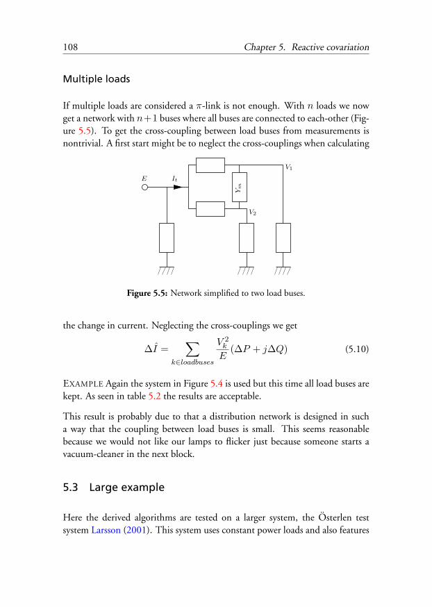
108 Chapter 5. Reactive covariation
Multiple loads
If multiple loads are considered a π-link is not enough. With n loads we nowget a network with n+1 buses where all buses are connected to each-other (Fig-ure 5.5). To get the cross-coupling between load buses from measurements isnontrivial. A first start might be to neglect the cross-couplings when calculating
V1
ItE
V2
Ym
Figure 5.5: Network simplified to two load buses.
the change in current. Neglecting the cross-couplings we get
∆I =∑
k∈loadbuses
V 2k
E(∆P + j∆Q) (5.10)
EXAMPLE Again the system in Figure 5.4 is used but this time all load buses arekept. As seen in table 5.2 the results are acceptable.
This result is probably due to that a distribution network is designed in sucha way that the coupling between load buses is small. This seems reasonablebecause we would not like our lamps to flicker just because someone starts avacuum-cleaner in the next block.
5.3 Large example
Here the derived algorithms are tested on a larger system, the Osterlen testsystem Larsson (2001). This system uses constant power loads and also features
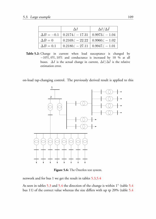
5.3. Large example 109
∆I ∆I/∆I
∆B = −0.1 0.2174 6 − 17.31 0.9973 6 − 1.04
∆B = 0 0.2169 6 − 22.22 0.9960 6 − 1.02
∆B = 0.1 0.2180 6 − 27.11 0.9947 6 − 1.01
Table 5.2: Change in current when load susceptance is changed by−10%, 0%, 10% and conductance is increased by 10 % at allbuses. ∆I is the actual change in current, ∆I/∆I is the relativeestimation error.
on-load tap-changing control. The previously derived result is applied to this
1
2
Figure 5.6: The Osterlen test system.
network and for bus 1 we get the result in tables 5.3,5.4
As seen in tables 5.3 and 5.4 the direction of the change is within 1 (table 5.4bus 11) of the correct value whereas the size differs with up tp 20% (table 5.4

110 Chapter 5. Reactive covariation
∆S/∆S
bus nr ∆Q = −0.1 ∆Q = 0 ∆Q = 0.1
3 1.0059 6 0.17 0.98946 0.25 0.9739 6 − 0.09
4 1.10816 − 0.10 1.06176 0.42 1.0163 6 − 0.38
5 1.10606 − 0.17 1.05496 0.44 1.0061 6 − 0.66
6 1.11446 − 0.18 1.06316 0.45 1.0134 6 − 0.55
7 1.11756 − 0.26 1.06166 0.47 1.0082 6 − 0.79
8 1.14326 − 0.46 1.07736 0.56 1.0110 6 − 0.54
9 1.11106 − 0.20 1.05846 0.45 1.0080 6 − 0.68
10 1.11146 − 0.25 1.05616 0.46 1.0039 6 − 0.84
11 1.14956 − 0.56 1.07636 0.62 1.0040 6 − 0.89
12 1.08626 − 0.15 1.04836 0.38 1.0103 6 − 0.21
14 1.09146 − 0.21 1.04406 0.44 0.9985 6 − 0.58
15 1.13196 − 0.45 1.07166 0.41 1.0129 6 − 0.81
16 1.11346 − 0.20 1.06776 0.36 1.0220 6 − 0.24
17 1.08896 − 0.19 1.04256 0.44 0.9979 6 − 0.55
all 1.09556 − 0.30 1.04846 0.24 1.0033 6 − 0.78
Table 5.3: Large example during low-load ∆P = −0.1
bus 11). This error in size is probably due to the fact that the loads are constant-power type loads whereas the calculations are derived assuming admittance-typeloads. Scaling the prediction so that the active part of the prediction equals theactive power that is switched makes the size prediction much better. This isequivalent to assuming a lossless line.
The combination that gives the best prediction is thus quite strange. The angleis given by assuming constant admittance type load and network with losses.Whereas the size is given by the amount of switched active load assuming losslesslines. The success of this scheme is most likely highly dependent on the operat-ing region and the changes in active/reactive power. One obvious case where itwill fail is when only reactive power is switched.

5.3. Large example 111
∆S/∆S
bus nr ∆Q = −0.1 ∆Q = 0 ∆Q = 0.1
3 1.0443 6 0.30 1.01676 0.46 0.9906 6 − 0.08
4 1.18566 − 0.36 1.10716 0.78 1.0278 6 − 0.39
5 1.17896 − 0.28 1.10556 0.75 1.0310 6 − 0.23
6 1.17846 − 0.30 1.10326 0.76 1.0272 6 − 0.32
7 1.14976 − 0.04 1.08786 0.71 1.0257 6 − 0.06
8 1.21006 − 0.91 1.11286 0.90 1.0104 6 − 0.23
9 1.17636 − 0.24 1.10526 0.74 1.0331 6 − 0.16
10 1.17926 − 0.40 1.09806 0.80 1.0171 6 − 0.61
11 1.22936 − 1.01 1.12836 0.91 1.0209 6 − 0.18
12 1.12676 − 0.14 1.08026 0.56 1.03196 0.27
14 1.12946 − 0.15 1.06976 0.71 1.0093 6 − 0.07
15 1.19136 − 0.68 1.11266 0.61 1.0312 6 − 0.31
16 1.19296 − 0.65 1.11676 0.58 1.0375 6 − 0.19
17 1.1106 6 0.15 1.06486 0.70 1.01846 0.29
all 1.15186 − 0.52 1.08546 0.40 1.0184 6 − 0.58
Table 5.4: Large example during high-load ∆P = −0.1
Analysis
The good agreement between when using constant impedence results for con-stant power type loads raises the question. Is this always true?
To try to answer this, a single load infinite bus system with a purely reactiveline is studied, Figure 5.7. This is a system commonly used in voltage stabilityanalysis see, Cutsem and Vournas (1998) and Taylor (1994).
In the following subscript r will be used for the receiving end and subscript s
for the sending end.

112 Chapter 5. Reactive covariation
E V 6 θ
P,Q
Figure 5.7: Single load infinite bus system.
The consumed active and reactive power is given by:
Pr = −E V Y sin(θ) (5.11)
Qr = E V Y cos(θ)− V 2 Y (5.12)
Solving this we get (assumes consumption of both active and reactive power)
V =
√Y E2 − 2 Qr +
√Y 2 E4 − 4 Qr Y E2 − 4 Pr
2
2 Y(5.13)
tan(θ) = − Pr
12 Y E2 + 1
2
√Y 2 E4 − 4 Qr Y E2 − 4 Pr
2(5.14)
Substituting this back into equations 5.11, 5.12 we get
Ps = Pr (5.15)
Qs =12
Y E2 − 12
√Y 2 E4 − 4 Qr Y E2 − 4 Pr
2 (5.16)
As the transmission is purely reactive we have dPsdPr
= 1 and dPsdQr
= 0. Theexpressions for the reactive variation are now given by
dQs
dPr=
2 Pr√Y 2 E4 − 4 Qr Y E2 − 4 Pr
2(5.17)
dQs
dQr=
Y E2√Y 2 E4 − 4 Qr Y E2 − 4 Pr
2(5.18)
The direction of the change in feeding power (∆Ss) is then given by
tan(arg(∆Ss)) =dQs
dPr
dPsdPr
=dQs
dPr(5.19)

5.3. Large example 113
comparing this with equation 5.14 it is noticed that if Y 2 E4 4 Qr Y E2 +4 Pr
2 then tan(arg(∆Ss)) ≈ 2 tan(θ) which for small θ gives arg(∆Ss) ≈2 θ.
0 0.1 0.2 0.3 0.4 0.50
0.05
0.1
0.15
0.2
0.25
Pr/SSC
Qr/S
SC
Figure 5.8: Level curves of the angular error obtained when using the approx-imation −2θ rather than arg( dSs
dPr) to calculate the direction of the
change in feeding power (∆Ss) when changing active load (Pr) as afunction of Pr, Qr. The spacing between the curves is 1, the thickline indicates the admissible operating region and the arrow indicatesthe direction in which the error increases.
A better view of the correctness of the estimate is seen in Figure 5.8 wherethe difference between the correct angle of ∆Ss and the estimated angle isplotted for a change in consumed active power, ∆Pr. As seen in this figure theapproximation is good when the consumed reactive power is small compared tothe consumed active power.

114 Chapter 5. Reactive covariation
5.4 Non-infinite bus
All the previous analysis has only concerned a distribution network connectedto an infinite bus. If instead the infinite bus is replaced by a Thevenin equivalentof the feeding system, then the system in Figure 5.9 is obtained. For this circuit
E
V1 V2ItYt1 Yt2
Y1 Y2
Figure 5.9: Thevenin source and π-link.
we have:
dIt
dY2=
V 22
E(5.20)
dV1
dY2= − dIt
dY2
1Yt1
= − V 22
E Yt1
(5.21)
where we notice that the expression for change in current is the same as derivedin section 5.2, the difference is that it now is the Thevenin source that is thereference. The circuit in Figure 5.9 can easily be transformed to a π-link by aY −∆ transform of Yt1 , Y1, Yt2 . The change in feeding voltage is just calculatedas the voltage drop across the internal impedance in the Thevenin equivalent.
The power injected into the π-link from the Thevenin equivalent is
S1 = V1 I∗t (5.22)
where ∗ denotes complex conjugate. Differentiating the above expression andsimplifying we get:
dS1
dY2= V1
d
dY2I∗t +
dV1
dY2I∗t = V1
(V 2
2
E
)∗− V 2
2
E Yt1
S1
V1(5.23)

5.4. Non-infinite bus 115
Inserting E = V1 + It Zt1 = V1 +(
S1V1
)∗Zt1 in the above equation we get
dS1
dY2= V1
V 22
V1 +(
S1V1
)∗1
Yt1
∗
− V 22
V1 Yt1 +(
S1V1
)∗ S1
V1(5.24)
Where the first term corresponds to a π-link connected to an infinite bus andthe second term can be seen as a correction for the voltage drop in the Theveninequivalent. With the same assumptions as earlier, the change in feeding powerat V1 is now given as
∆ S1 =dS1
dY2(∆P + j∆Q) (5.25)
For constant power type loads in a reactive network, it is, as described in section5.3, normalize the real part of dS1
dY2or the real part of dIt
dY2to achieve better
results. For the studied cases, the difference between the two normalizations isinsignificant.
An alternate way to calculate the change in feeding power is to use
∆ S1 = (V1 + ∆V1) (It + ∆It)∗ − S1 (5.26)
Again, the difference in the results between this formulae and equation (5.25)is minimal.
When these results are applied to the system in Figure 5.6, then for bus 2 weget the results in tables 5.5 and 5.6

116 Chapter 5. Reactive covariation
∆S/∆
S
bus
nr∆
Q=−
0.1
∆Q
=0
∆Q
=0.1
31.0
36260.3
11.0
30460.2
71.0
25560.0
9
41.0
84460.2
01.0
51160.4
41.0
1986−
0.2
8
51.0
84160.2
01.0
47960.4
61.0
1536−
0.4
9
61.0
87860.1
81.0
50960.4
61.0
1696−
0.4
2
71.0
89860.1
51.0
49760.4
91.0
1386−
0.6
0
81.1
1936−
0.0
41.0
67460.5
81.0
1726−
0.4
8
91.0
86560.1
81.0
49060.4
71.0
1516−
0.5
1
101.0
87160.1
71.0
47860.4
81.0
1326−
0.6
3
111.1
2306−
0.0
71.0
65660.6
41.0
1166−
0.7
6
121.0
75660.1
11.0
50460.3
91.0
2596−
0.0
8
141.0
78460.1
51.0
46260.4
51.0
1706−
0.3
8
151.0
9766−
0.0
41.0
53060.4
11.0
1186−
0.6
8
161.0
87860.0
71.0
53960.3
61.0
2106−
0.2
2
171.0
77260.1
71.0
45960.4
51.0
1746−
0.3
5
all
1.0
82860.0
81.0
49060.3
31.0
1826−
0.5
1
Tabl
e5.
5:La
rge
exam
ple
duri
nglo
w-l
oad
∆P
=−
0.1
∆S/∆
S
bus
nr∆
Q=−
0.1
∆Q
=0
∆Q
=0.1
31.0
32060.5
91.0
22260.5
01.0
14060.1
7
41.1
15160.3
11.0
59460.8
21.0
0676−
0.3
7
51.1
11660.3
41.0
59560.7
91.0
0976−
0.2
4
61.1
11660.3
41.0
58460.8
01.0
0796−
0.3
1
71.0
97160.4
71.0
54160.7
41.0
1316−
0.0
7
81.1
6256−
0.1
21.0
86060.9
51.0
0976−
0.3
7
91.1
10160.3
51.0
59760.7
81.0
1136−
0.1
8
101.1
12860.3
31.0
55760.8
31.0
0286−
0.5
4
111.1
7146−
0.2
11.0
91560.9
61.0
1116−
0.3
4
121.0
89360.2
31.0
58660.5
81.0
27560.2
5
141.0
90860.3
71.0
50760.7
31.0
1236−
0.0
3
151.1
1976−
0.0
41.0
62960.6
31.0
0726−
0.3
8
161.1
2016−
0.0
51.0
64660.6
01.0
0986−
0.2
9
171.0
80760.5
11.0
50360.7
11.0
20560.2
7
all
1.1
03560.1
71.0
56460.5
81.0
1156−
0.3
9
Tabl
e5.
6:La
rge
exam
ple
duri
nghi
gh-l
oad
∆P
=−
0.1

5.5. Large disturbance analysis 117
5.5 Large disturbance analysis
The previous analysis has only been concerned about small disturbances. In thissection we try to answer the question if it is possible to predict the behaviour forlarge disturbances without solving the complete load-flow problem. We keepthe assumption made earlier, that is, only one feeding voltage and admittancetype loads.
First, recall equation 5.3 for the reduced system.
V1 =
[Vf
V
]I1 =
[If
0
]YrV1 = I1 (5.27)
Modifying the above equation into standard shape we get
Y
[If
V
]=
[Vf
0
](5.28)
Solving for the feeding current and substituting it back into equation (5.28) weobtain
If = Y−111
(Vf − Y12V
)(5.29)
Y21Y−111 Vf︸ ︷︷ ︸
b
=(Y21Y−1
11 Y12 − Y22
)︸ ︷︷ ︸
A
V (5.30)
This substitution transforms the circuit to only contain load buses. The feedingvoltage is replaced with current injections at all buses. We would now like toknow how the solution (V ) changes when the modified admittance matrix ischanged, that is
b = (A + δA)(V + δV ) (5.31)
and where b represents the feeding voltage. A whole class of disturbances cannow be applied to the modified admittance matrix, disturbances that have alimited norm, ||δA|| < C. This can be interpreted as a number of disturbancesthat all have absolute value smaller than C. If the load-admittance varies muchbetween the load buses it makes sense to scale the equations. The only way

118 Chapter 5. Reactive covariation
of scaling that has been tried is to make the real part of the diagonal elementsequal, for example 1. With 0 < C < 1 this can now be seen as a relativedisturbance. Using norms for the disturbance means that there is no control onwhere non-zero elements show up is the disturbance of the admittance matrix.This means that there can be non-physical disturbances such as the admittanceof a line being different in different directions. It is thus a very coarse andgeneral description of the potential disturbances.
Applying the following inequality on the disturbed system (equation 5.31),where κ(A) denotes the condition number of A,∣∣∣∣∣∣δV ∣∣∣∣∣∣∣∣∣∣∣∣V ∣∣∣∣∣∣ ≤ 1
1− κ(A) ||δA||||A||
κ(A)||δA||||A||
(5.32)
it is now possible to use the result backwards and calculate the norm of themaximal change in current.
δIf = −Y−111 Y12δV (5.33)
||δIf || ≤∣∣∣∣∣∣Y−1
11 Y12
∣∣∣∣∣∣ ∣∣∣∣∣∣δV ∣∣∣∣∣∣ (5.34)
As it is only possible to calculate the norm of the change, there is no way to tellwhich direction the change will have. The answer is an upper bound on thechange in feeding current/power.
5.6 Conclusions
It has been shown that the ability to predict the change in feeding power (activeand reactive) to a distribution network when a small load is switched furtherdown is closely related to the angular difference of the voltages at the load busand the feeding bus. For admittance type loads the size of the change is givenby the voltage levels at the load bus and the feeding bus. The main advantagewith the method is that no network model is needed if phasor measurements areavailable. If phasor measurements are lacking, a load-flow combined with theoutlined method will give the same result as with phasor measurements but witha computational cost that is much lower than repeated load-flow calculations.

5.6. Conclusions 119
The theory is developed for constant admittance type loads but works well onconstant power type loads provided that consumed active power is much largerthan consumed reactive power and that we are operating far from transmissionlimits.
Given that the coupling between loads is small the results can also be used whenseveral loads are switched, although the result is not as accurate as for a singleload.
When large loads are switched it is possible to determine the size of the changein feeding power but not the direction. Furthermore a detailed network modelis needed. The cost of the computations needed to get the result might be muchhigher than the cost of a number of load-flows.
At present only networks fed from a single source are treated. It is possible toextend the results for multi-source networks. This will, however, require moreknowledge about the network.

120 Chapter 5. Reactive covariation

Chapter 6
Distributed load control fordamping enhancement
The goal of this chapter is to illustrate how the results from the previous chapterscan be used to achieve damping enhancement by distributed control of activeload. In Samuelsson and Eliasson (1997); Samuelsson (1997) it was shown thatcontrol of active power at the transmission network level enhances the dampingof the electro-mechanical modes. In this chapter, the behaviour when using theload in the distribution network as actuators will be investigated. The chapterstarts with a section about load control and ends with case studies of the threemachine system in Anderson and Fouad (1993) and a 16-machine model of theNORDEL power system, Akke (1989).
6.1 Active load control
In this section different control strategies and ways to implement load-controlis described. Furthermore, characteristics for loads suitable for load-control arediscussed. Finally the size of a distributed actuator is discussed.
121

122 Chapter 6. Distributed load control for damping enhancement
Loads
As few loads, suitable for load control, are connected directly to the transmis-sion network there is a need to decentralize the loads as control elements. A loadsuitable for load control should typically consume little or no reactive power andhave a dynamics that is much slower than the electro-mechanical dynamics. Itis also advantageous if the load have a “constant energy” type behaviour. Themotivation for the first requirement is that the reactive variation when loads areswitched on or off should be small. For a purely active load the only contri-bution to reactive variation will then be the contribution from the distributionnetwork. The second requirement is motivated by the acceptance to loss ofpower. With load dynamics much slower than the electro-mechanical dynam-ics, a short disconnection of an operating load will be almost unnoticeable. Theargument for the third requirement is that it simplifies pricing of the dampingservice. If a load consumes the same amount of energy, no matter if it is usedfor damping or not, then the producing companies need not be compensatedfor loss of production.
A load category that fulfils all the requirements are resistive heating loads suchas residential water heaters, coffee machines, electric heating, electric cookersand resistive furnaces. Also electric district heating boilers can be consideredbut they are rare and not always in operation. Other plausible loads are power-electronically controlled loads that can be allowed to change their setpoint. Thiscan include pump and fan drives as well as battery chargers. Loads unsuitablefor load control are for example refrigerators that have a motor which is directlyconnected to the grid.
Control strategies
Load control is usually a quantized type of control, that is the control signal ischanged in steps rather than continuously. This together with the fact that itis energy that should be removed/added to the generators implies that as muchpower as possible should be used in order to give a high control authority. Inthe rest of this section we will therefore assume on-off control.
Control systems can be divided into feedback and feed-forward/precomputed

6.1. Active load control 123
control.
In feedback control measurement or quantities estimated from measurementsare used as inputs to a controller. Advantages with this type of control are thatthe system is continuously monitored and that the effects of the control actionis directly visible to the controller. A power system is conveniently described bya differential algebraic (DAE) system. The algebraic part implies that there aredirect connections between controlled and observed quantities. Here, there willbe a direct connection between load and phase-angle. Using local frequency,which is the time derivative of the phase-angle, as controller input implies thatthe frequency measurement must be done with care in order to avoid largedisturbances in the measurements.
One way to avoid this is to use a precomputed control signal. With this ap-proach, once the sequence is started there is no need to calculate estimates asthe estimates will not influence the control. The control signal can easily beextracted from the outputs of a damping estimator by making a square wavecontrol action with the same frequency as the mode that should be damped.The frequency and damping are given by the estimator. The sequence is thenstarted a zero crossing of the measured signal. The main advantage with thisapproach is simplicity. Drawbacks are that only single mode systems are thiseasy to handle. With on-off control it is only the signal of the observed quant-ity that is of interest. A multi mode oscillation will not have only one frequencyand to synthesize a control signal from several observed modes is impossible asthere is no information about the phase and amplitude of the different modes.Furthermore, applying control will not change the frequency of the oscillationbut rather its phase. If a long control signal is pre-computed it might end withthat the control signal and the actual monitored signal are out of phase, leadingto excitation rather than damping of the system.
Centralized – Decentralized control
Load control for damping enhancement as performed in Samuelsson (1997)suggests the following quantities as suitable feedback signals:
• local bus frequency

124 Chapter 6. Distributed load control for damping enhancement
• frequency of the closest machine
• estimated mode frequency
For a centralized damping controller, which is a controller that has access totransmission level measurements, all the suggested quantities can be used. Thisapproach will probably achieve the highest performance but the requirementson communication bandwidth is high. The communication requirements canbe summarized as:
• System measurements need to be brought to the controller.
• Loads need to send their status, telling the controller how much dampingpower they have available.
• Control actions need to be communicated to the loads.
One issue with a centralized controller is the time delay introduced by the com-munication. To get high performance this delay should be kept small or con-sidered in the control design. It can be argued that todays fast communicationlike the internet should be fast enough. Looking at the capacity of a commu-nication link this is generally true. The capacity is, however, the capacity duringideal circumstances. This often means that there are few hosts on the networkand that the data is sent in large packets. In a control system, the data is typic-ally one measurement sent at an fixed interval. This means that the data packetsare small giving a large overhead for the protocol part of the transmission. Also,the number of hosts will be large, at least one for each load and one for eachmeasurement site.
In a decentralized system, measurements and control action are performed atthe same place, locally. While removing the need of communication there isnow an increase in the number of required measurement units (one for eachload). Also, the number of quantities suitable as feedback signals are reducedto local frequency. With a decentralized system there is also the possibility ofthe different control loops counteracting each other as only local data are avail-able. The effect of counteraction be minimized by proper selection of controlparameters but this is against the whole idea with a decentralized system. Onecase where this is clearly visible is tap changer control in distribution networks.

6.1. Active load control 125
In Larsson (2001) it was shown that the number of tap-changing operations ina radial network could be reduced by 45% while maintaining a better voltageprofile when introducing a centralized controller.
A mixture of the two extremes could prove useful in that the requirements oncommunication capacity is relieved while maintaining some coordination andkeeping the number of measurement units down. A possible scenario is tolocate the measurement and control equipment in a substation. Control signalsare then sent on the power lines to the loads. In case of on-off control this isparticularly convenient as only two different kind of messages (on or off ) needto be sent. Advantages with this solution are
• Simple interface to actuators
• Limits counteraction
• Limits sensitivity to communication/hardware problems compared to cent-ralized system.
• Number of measurement units small and hopefully of better quality com-pared to decentralized system.
Actuator sizing
Given that an area is equipped with controllable loads, what is the size of thecompound actuator and what is the size affected by? The maximal capacity ofthe actuator is given by the total amount of load with control equipment in-stalled. The possibility to use the maximal rating is heavily dependent on thetypes of loads and how they are allowed to operate. Comparing load-controlwith load-shedding we conclude that it is always allowed to disconnect oper-ating loads and then reconnect them again. The reverse, to engage a load thatinitially is off is more dependent on the type of load. Residential water heatersfor example, can probably be turned on although the water is sufficiently hot.Electric cookers on the other side, should probably not be turned on except forparts that happens to be in use at the moment.
The size of the actuator can thus vary considerably depending on load compos-ition, allowed switching and initial state of the individual loads.

126 Chapter 6. Distributed load control for damping enhancement
Another question that needs to be answered is how much of the available powershould be used for damping purposes. If damping power is free, then everythingthat can be used to achieve a high damping can be used. The reactive covariationwill counteract the desired action caused by the active load. However, as longas the reactive covariation is small compared to the active variation, a higherdamping is achieved with larger control-power. The bottom part of Figure 6.6illustrates the influence of reactive covariation.
When there is a cost associated with damping power there will be a trade-offbetween the cost of additional damping versus the usefulness of the increaseddamping. In such a scenario, the price of damping power will be determinedby the need of damping power versus the availability and quality of dampingpower, where high quality power has low reactive covariation.
Who can supply the damping power? Technically, the damping power is sup-plied by the end user. From a market perspective the damping power can besupplied either by the end user, the transmission system operator or a distribu-tion company. In all cases it is the person/organization that makes the invest-ments in equipment for load control that should be seen as the seller of dampingpower.
For a truly decentralized system without communications the damping powerprovider is probably the end consumer or the transmission system operator.The high accuracy requirement on the damping detector will make the detectorexpensive. This will probably limit control installations to large loads. To get ahigh penetration of control equipment on smaller loads the damping detectorwill need to be cheap or subsidized. Even with cheap detectors it will take longtime before the penetration of controlled loads is high as the cost in upgradingthe equipment will be substantial.
When having a system that relies on communication between the loads and acentral controller, the distribution companies can enter the damping market.In this case the distribution company typically has communications for remotemetering and possibly also for broadband connections. The idea now is to con-nect suitable loads such as heating loads to outlets that can be controlled by thedistribution company. The distribution company can now sell controllable loadto the transmission system operator. The end customer can be compensated bya lower tariff or energy price.

6.2. Case studies 127
In all cases, it is hard to estimate the amount of power available for control.For a centralized system one can envision a system where the loads send theirrespective state to the controller. The central controller will then act not onlyas a controller but also as a load-dispatcher that can select a suitable amount ofload to use.
6.2 Case studies
The on-off control strategy is evaluated on two test cases, the three-machine sys-tem in Anderson and Fouad (1993) and a 16-machine system of the NORDELnetwork. The main goal with these studies is to study the impact the reactivecovariation has when using load-modulation for damping enhancement. Re-active covariation comes from the distribution network. These networks are,however, not modelled in detail in the simulations. Instead, the results fromthe previous chapter is used to mimic the behaviour of load-modulation in adistribution network.
The controllers use local bus frequency as their input signal. Thus no estimationof the damping or oscillation frequency is performed.
Three-machine system
A three machine system has two oscillatory electro-mechanical modes and thusforms the first step towards a general multi-machine system. The nine bussystem of Anderson and Fouad (1993), also known as the WSCC 9 system,is selected for having the generic meshed network with one mesh, Figure 6.1.The generators are modelled by third order models without damper windingsand the magnetization is controlled by a proportional AVR measuring terminalvoltage. The mechanical input power is kept constant. The loads are equippedwith load control using local frequency as input.
For the studied load case the system has two modes, one at 1.3 Hz and one at1.8 Hz. In the 1.3 Hz mode the generators at buses 2 and 3 swing against thegenerator at bus 1. In the 1.8 Hz mode the generator at bus 2 swings againstthe generator at bus 3.

128 Chapter 6. Distributed load control for damping enhancement
1
4
5 6
7 8 9 32
Figure 6.1: The Andersson-Fouad test system
With the loads located approximately halfway between the generators we canexpect both mode observability (from frequency) and mode controllability tobe small.
At 5s the system is excited by a fault at bus 8 which is removed after 0.1s. InFigure 6.2 the frequency deviations at the loads are seen.
Introducing damping by means of load control at all load busses increases thedamping significantly as seen in Figure 6.3. In this case the active modulationwas 5% of the load at each bus and no reactive covariation. Although thefrequency deviation decays it settles with a peak value of at most 0.1 Hz. Thislarge value can be explained by looking at the frequency deviation at the loadbusses (Figure 6.4). There it is seen that the frequency deviation at the loadbusses is small making the remaining oscillation invisible for the control system.
This is a structural problem that can only be solved by using other signals asfeedback signals or by relocating the loads.

6.2. Case studies 129
-0.3
-0.2
-0.1
0
0.1
0.2
0.3
0 2 4 6 8 10 12 14
f [H
z]
time [s]
load 8load 6load 5
Figure 6.2: Load frequency deviation with no additional damping.
-0.3
-0.2
-0.1
0
0.1
0.2
0.3
0 2 4 6 8 10 12 14
f [H
z]
time [s]
gen 3gen 2gen 1
Figure 6.3: Generator frequency deviation with damping by load control.
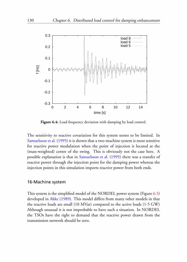
130 Chapter 6. Distributed load control for damping enhancement
-0.3
-0.2
-0.1
0
0.1
0.2
0.3
0 2 4 6 8 10 12 14
f [H
z]
time [s]
load 8load 6load 5
Figure 6.4: Load frequency deviation with damping by load control.
The sensitivity to reactive covariation for this system seems to be limited. InSamuelsson et al. (1995) it is shown that a two-machine system is most sensitivefor reactive power modulation when the point of injection is located at the(mass-weighted) centre of the swing. This is obviously not the case here. Apossible explanation is that in Samuelsson et al. (1995) there was a transfer ofreactive power through the injection point for the damping power whereas theinjection points in this simulation imports reactive power from both ends.
16-Machine system
This system is the simplified model of the NORDEL power system (Figure 6.5)developed in Akke (1989). This model differs from many other models in thatthe reactive loads are small (10 MVar) compared to the active loads (1-5 GW)Although unusual it is not improbable to have such a situation. In NORDELthe TSOs have the right to demand that the reactive power drawn from thetransmission network should be zero.

6.2. Case studies 131
12
13
11
6
15
16
10
14
9
8
5
1
2
3
4
7
Figure 6.5: The 16-bus NORDEL test system. The area of the busses corres-ponds to the amount of stored energy in the generators connected tothat bus. For each of the lines, the width of the line corresponds tothe admittance of that line; thick line = short electrical distance.

132 Chapter 6. Distributed load control for damping enhancement
Simulation setup
The generators are described by third order models. All generators are equippedwith voltage controllers but PSSs are turned off in order to get a more oscillatorysystem. All loads are equipped with load control using local frequency as input.The amount of load used for control is 2% or 4% of the active load at eachload bus. The reactive variation is 0, 25%, 50% or 75% of the active variation.From Chapter 5 we find that for small deviations, the change in apparent powerhas a direction of 5 − 15. With 50% reactive covariation, corresponding tothe change in apparent power having an angle of 28 this should be more thanenough to cover a worst case scenario.
The system is excited at 10s by a fault on the line between bus 5 and bus 6(southern Norway). The fault is removed after 0.1s and the power on the linebetween bus 5 and bus 11 (grey in Figure 6.5) is studied.
Analysis
In Figure 6.6 (top) it is seen that the damping is increased considerably whenusing only 2% of the load power for damping enhancement. It can also beseen that the system is sensitive to reactive covariation. For the studied case, thereactive covariation deteriorates the performance compared to a case withoutreactive covariation. Comparing the results from the case without additionaldamping and additional damping with reactive covariation, we notice that theresult with reactive covariation is still superior to the case without additionaldamping.
Increasing the amount of damping power to 4% of the total load the dampingis further increased. Comparing 4% active load and 50% reactive covariationwith 2% active load and no reactive covariation (Figure 6.6 bottom) it is seenthat the increased damping is only visible during the first 4 swings. After thisthe two cases behave quite similarly. Keeping the reactive covariation small isthus an important goal as it will allow the controller to use a smaller amount ofpower.

6.2. Case studies 133
−2000
−1500
−1000
−500
0
500
0 5 10 15 20 25 30 35 40
po
we
r [M
W]
time [s]
no damping∆P = 2%,∆Q = 0
∆P = 2%,∆Q = ∆P/2
0 10 20 30 40−2000
−1500
−1000
−500
0
500
time [s]
pow
er
[MW
]
no damping∆P = 2%, ∆Q = 0
∆P = 4%, ∆Q = ∆P/2
Figure 6.6: Power oscillations on one connection between Sweden and Norway.

134 Chapter 6. Distributed load control for damping enhancement
6.3 Conclusions
It has been shown that applying load control based on local frequency meas-urements increases the damping in the two test cases. The influence of reactivecovariation is largely dependent on network topology and load location. Thepractical influences of the reactive covariation is governed by the cost of damp-ing power and control equipment in that low-cost power and equipment re-duces the need of small reactive covariation. When small reactive covariationis required, local control is infeasible as prediction of reactive covariation re-quires local system knowledge and thus communication. Actuator location isalso important for reactive covariation. In Samuelsson (1997) it is argued thatthe dampers should be located as close as possible to the swinging generators. Incase this is unfeasible actuator location can be studied by the method describedin Smed (1993).
Controller interaction is not studied. Although it is highly probable that betterdamping can be achieved by only using a few dampers, the results obtained withdampers at all nodes is superior to the poorly damped cases.
The use of load control is only useful for damping enhancement. The influenceon transient stability is non existent due to the amount power used for dampingis much smaller than the power in the swings.
Implementation of one of the proposed schemes depends largely on what pay-back one can expect and what kind of load that is chosen. For residential loads,a variant with a controller at the closest transformer is probably the cheapest.The controller will then send two different frequencies on top of the funda-mental frequency, one frequency to turn on load and one to turn off load. Theexpensive part will then be in the transformer station whereas the additionalcost for the appliances to be controlled can be held low.

Chapter 7
Concluding remarks
The topic of this thesis is power system oscillations and more precisely, howto minimize the effects of the oscillations. Oscillations are studied in differenttimescales, each one requiring its own treatment. First a summary of the ob-tained results is given. Second, some topics for future research in the area ofpower system oscillations are provided.
7.1 Summary of results
Detection
Swing detection strives to answer the question; is the present situation due to apower swing? Detection of power swings is a slow process since a power swingis a slow phenomenon compared to faults. For fast response it is often feasibleto rephrase the question into; is the present situation caused by a fault? Inthis context, a power swing is regarded as a normal albeit undesirable operatingcondition. Based on this, a new idea for distinguishing faults from power swingsin distance protection relays is presented. The principle is based on a changeof coordinate system to a system that is more suitable for distinguishing faultsfrom power swings. It should be noted that the proposed method only worksfor large power swings, that is, when there is a risk to mix up faults with powerswings. The new detector performs well for low impedance faults in a line. In
135
136 Chapter 7. Concluding remarks
case of parallel lines and low impedance faults the detector on the faulted linewill indicate a fault. The detector on the parallel healthy line will, however, notalways detect the situation as a fault. This is due to the location and impedanceof the fault together with source impedances.
Estimation
Estimation of the frequency and damping for the electro-mechanical modes in apower system can be performed on data from large disturbances, ring down ana-lysis, or from data collected during normal operation, ambient analysis. Bene-fits with ambient analysis is the possibility to get information about the systemwithout probing it. This can be used for planning studies and model calibra-tion. The use of ambient analysis also makes real-time monitoring of oscillationfrequency and damping possible. Detection of low damping can then alarm op-erators or enable special protection schemes. A drawback with ambient analysisis that the system might be poorly excited making it difficult to estimate theparameters.
It is shown in case studies on measured data that real-time monitoring of electro-mechanical oscillation frequency and damping is possible, at least for singlemode systems. It is also discussed that the interpretation of the results are ofteneasier to perform in the frequency domain rather than using pole locations. Forvery lightly damped systems it is, however, possible to evaluate the system fromthe pole locations only. Using spectral estimates does, however, contribute a lotto the general understanding of the system behaviour.
Damping estimation can be done from any system wide measured quantity.For load-control it interesting to use local frequency as an indicator of poorlydamped dynamics. Limits on resolutions are derived and compares well tomeasurements.
Control
Control of active power on end-user loads in order to enhance the damping oflightly damped electro-mechanical modes in a power system is pursued. For thecontrol to be effective, the variation of reactive power at the transmission level

7.2. Future work 137
should be kept small while the variation of active power should be large. Thedistribution network will, however, contribute with some change in reactivepower when active end-loads are changed.
The change in reactive power contributed by the distribution network is stud-ied. In the timescale of a power swing, admittance type load behaviour can beexpected. For this case it is shown that the angle between the positive sequencevoltages at the load and the feeding bus is a good measure of the reactive cov-ariation. It is also shown when this approximation is valid for constant powertype loads. When evaluated on a test system, the accuracy for changes at leastup to 10% is good.
The results derived above are used to mimic the behaviour of distribution net-works subject to end-load control when simulating transmission system beha-viour. Two systems are investigated, a three-machine test system and a 16-machine system derived from the NORDEL system. For both cases, the damp-ing is considerably enhanced when using load modulation based on local busfrequency.
The three-machine system is relatively insensitive to variations in reactive power.The sensitivity to variations in active power is, however, also limited. The latterbehaviour is due to the location of the loads being close to the (mass-weighted)centre of the swing modes. This also reduces the mode observability.
The 16-machine system is sensitive to reactive variation, the performance is,however, not severely deteriorated. The sensitivity to active variations is highwhich can be seen from the fact that using only 2% of the available active loadfor load modulation enhances the damping significantly. Even when the reactivecovariation is increased to unreasonable levels, the performance compared to thecase without load modulation is superior.
7.2 Future work
The detection algorithm is derived under the simplified assumption that theapparent impedance moves on a circle. As seen in the case studies it works welleven on multiple circles and “close to circles” (poleslipping). The performanceneeds, however, to be evaluated on more realistic data. The detector today is

138 Chapter 7. Concluding remarks
only a fault/non-fault detector. The possibility to predict out-of-step conditionsshould be investigated. This can be done by using the angle formed by the linesbetween the origin and the circle centre and the circle centre and the impedance.This angle is a measure of the angle between the generator and the centre ofinertia. The angle and its derivative could then be used in the same way asgenerator angle and speed to predict a pending loss of synchronism.
The techniques used to estimate frequency and especially damping can be de-scribed as brute force methods. As shown here and in Wies et al. (2003) determ-ination of damping is difficult, especially when damping is high or excitation islow. Fundamental limits on when damping estimation is possible would proveuseful and will possibly give insight to better methods to estimate damping.The driving forces for small oscillations, that is the random load variations,should be investigated. So far white noise has been assumed which probably is apoor assumption. More work in the spirit of Johansson and Martinsson (1986)needs to be done in order to tune the estimators. Estimators using more thanone input signal should be investigated in order to see what benefits that can begained in accuracy and estimation speed.
Load control is simulated with loads mimicing the behaviour of an aggregatedload subject to load modulation. More detailed analysis should be performedin order to verify the behaviour of the aggregated load. This should also includedynamic loads as the dynamics of loads can influence the damping substantiallywhich can be seen in Hiskens and Milanovic (1997). For local control the needof high precision frequency measurements where the signal is subjected to phasejumps needs to be addressed.

Bibliography
PES Winter Meeting (2000). IEEE Power Engineering Society Winter Meeting.Conference Proceedings. 140, 142
Akaike, H. (1974). A new look at the statistical model identification. IEEETransactions on Automatic Control , vol. 19, no. 6, pp. 716–723. 53
Akke, M. (1989). Power System Stabilizers in Multimachie Systems. Lic Thesis,Dept of Automatic Control, Lund University, Sweden. 121, 130
Anderson, P. M. and Fouad, A. A. (1993). Power System Control and Stability.IEEE. 121, 127
Bendat, J. S. and Piersol, A. G. (1980). Engineering Applications of Correlationand Spectral Analysis. John Wiley & sons. 42
Bounou, M., Lefebvre, S. and Malhame, R. (1992). A spectral algorithm forextracting power system modes from time recordings. IEEE Transactions onPower Systems, vol. 7, no. 2, pp. 665–683. 60
Cao, L. and Schwartz, H. M. (2000). A directional forgetting algorithm basedon the decomposition of the information matrix. Automatica, vol. 36, no. 11,pp. 1725–31. 30, 65, 66, 82, 87
Centeno, V., de la Ree, J., Phadke, A., Michel, G., Murphy, R. and Jr., R. B.(1993). Adaptive out-of-step relaying using phasor measurement techniques.IEEE Computer Applications in Power, vol. 6, no. 4, pp. 12–17. 21
Centeno, V., Phadke, A., Edris, A., Benton, J., Gaudi, M. and Michel, G.(1997). An adaptive out-of-step relay [for power system protection]. IEEETransactions on Power Delivery, vol. 12, no. 1, pp. 61–71. 21
139

140 Bibliography
Chui, C. K. and Chen, G. (1999). Kalman Filtering with Real-Time Applica-tions. Springer Series in Information Sciences.Vol. 17. Springer. 67
Claesson, I., Eriksson, P., Mandersson, B. and Salomonsson, G. (1990). AnalogCircuits and Signals. Studentlitteratur. In Swedish. 48
Clarke, E. (1945). Impedances Seen by Relays during Power Swings with andwithout Faults. AIEE Transactions, vol. 64, pp. 372–384 +471–472. 14, 21
Cutsem, T. V. and Vournas, C. (1998). Voltage Stability of Electric Power Systems.Kluwer Academic Publishers. 111
Dash, P. K., Pradhan, G. P. A. K., Routray, A. and Duttagupta, B. (2000). Anextended Kalman filter for frequency measurement of distorted signals. InPES Winter Meeting (2000). 67
Dous, G. L. (1999). Voltage stability in power systems. Lic Thesis, Dept ofElectric Power Systems, Chalmers Goteborg Sweden. 101
Goodwin, G. C. and Payne, R. L. (1977). Dynamic System Identification, Ex-periment Design and Data Analysis. Academic Press. 26
Haner, J., Laughlin, T. and Taylor, C. (1986). Experience with the R-Rdotout-of-step relay. IEEE Transactions on Power Delivery, vol. PWRD-1, no. 2,pp. 35–39. 12, 17
Hansson, M. and Salomonsson, G. (1997). A multiple window method forestimation of peaked spectra. IEEE Transactions on Signal Processing , vol. 45,no. 3, pp. 778–781. 58
Hauer, J., Demeure, C. and Scharf, L. (1990). Initial results in prony analysisof power system response signals. IEEE Transactions on Power Systems, vol. 5,no. 1, pp. 80–9. 41
Hauer, J., Hughes, F. J., Trudnowski, D., Rogers, G., Pierre, J., Scharf, L. andLitzenberger, W. (1998). A Dynamic Information Manager for NetworkedMonitoring of Large Power Systems. Tech. Rep. WO 8813-01, EPRI. 42
Hemmingsson, M. (2001). Estimation of Electro-Mechanical mode parametersusing frequency measurements. Tech. Rep. TEIE-7141, Dept of IndustrialElectrical Engineering & Automation, Lund University, Sweden. 6

Bibliography 141
Hemmingsson, M., Samuelsson, O., Pedersen, K. O. H. and Nielsen, A. H.(2001). Estimation of electro-mechanical mode parameters using frequencymeasurements. In IEEE Power Engineering Society Winter Meeting. ConferenceProceedings. 6
Hill, D. J. (1993). Nonlinear dynamic load models with recovery for voltagestability studies. IEEE Transactions on Power Systems, vol. 8, no. 1, pp. 166–176. 101
Hiskens, I. and Milanovic, J. (1997). Locating dynamic loads which signific-antly influence damping. IEEE Transactions on Power Systems, vol. 12, no. 1,pp. 255–262. 4, 138
Ilar, F. (1981). Innovations in the detection of power swings in electrical net-works. Brown Boveri Review, vol. 68, no. 2, pp. 87–93. 15
Ilar, F. and Metzger, F. (1984). European patent no 0 057948 b1, us patent4,426,670. 15
Johansson, K. and Martinsson, B. (1986). Measurement and Validation of Load-Variations. Master’s thesis, Dept of Electric Power Systems, Chalmers Gote-borg Sweden. in Swedish. 43, 49, 50, 97, 138
Johansson, R. (1993). System Modeling and Identification. Englewood Cliffs,N.J. Prentice Hall. 98
Jonsson, M. and Daalder, J. (2001). A new protection scheme to prevent mal-trips due to power swings. In 2001 IEEE/PES Transmission and DistributionConference and Exposition, vol. 2, pp. 724–730. IEEE. 17
Julier, S. J. (1997). Process Models for the Navigation of High-Speed Land Vehicles.Ph.D. thesis, University of Oxford, England. 67
Karlsson, D. and Hill, D. J. (1994). Modelling and identification of nonlineardynamic loads in power systems. IEEE Transactions on Power Systems, vol. 9,no. 1, pp. 156–166. 49, 101
Kautz, W. H. (1951). Transient synthesis in time domain. IRE Transactions onCircuit Theory, vol. 1, no. 3, pp. 29–39. 56

142 Bibliography
Kosterev, D. N., Taylor, C. W. and Mittelstadt, W. A. (1999). Model validationfor the august 10, 1996 wscc system outage. IEEE Transactions on PowerSystems, vol. 14, no. 3, pp. 967–979. 89, 95, 97
Kumaresan, R. and Tufts, D. W. (1982). Estimating the parameters of exponen-tially damped sinusoids and pole-zero modeling in noise. IEEE Transactionson Acoustics, Speech, and Signal Processing , vol. 30, no. 6, pp. 833–40. 52, 53
Lacoss, R. (1971). Data adaptive spectral analysis methods. Geophysics, , no. 36.57
Larsson, M. (2001). Coordinated Voltage Control in Electric Power Systems. Ph.D.thesis, Dept of Industrial Electrical Engineering & Automation, Lund Uni-versity, Sweden. http://www.iea.lth.se/publications. 108, 125
Ledwich, G. and Palmer, E. (2000). Modal estimates from normal operation ofpower systems. In PES Winter Meeting (2000), pp. 1527–31. 43, 79
Lee, K. and Poon, K. (1988). Analysis of transient swings in large intercon-nected power systems by Fourier transformation. IEEE Transactions on PowerSystems, vol. 3, no. 4, pp. 1573–1579. 62
Lee, K. and Poon, K. (1990). Analysis of power system dynamic oscillationswith beat phenomenon by Fourier transformation. IEEE Transactions onPower Systems, vol. 5, no. 1, pp. 148–153. 62
Ljung, L. and Soderstrom, T. (1983). Theory and Pratice of Recursive Identifica-tion. The MIT Press Cambridge, Massachusetts. 65, 98
Machowski, J. and Nelles, D. (1992). Deutsches patent de 41 00 646 a1. 15
Machowski, J. and Nelles, D. (1997). New power swing blocking method.In Sixth International Conference on Developments in Power System Protection.IEE. 15
Middleton, R. and Goodwin, G. (1990). Digital Control and Estimation, -aUnified Approach. Prentice Hall. 56
Minakawa, T., Sato, M., Ichikawa, Y. and Ishihara, Y. (1999). A new methodfor detecting loss of synchronism using power and current measured on aline. IEEE Transactions on Power Delivery, vol. 14, no. 1, pp. 68–73. 19, 20

Bibliography 143
Moore, P. and Johns, A. (1996). New method of power swing blocking for di-gital distance protection. IEE Proceedings Generation, Transmission and Dis-tribution, vol. 143, no. 1, pp. 19–26. 16
Murthi, M. N. and Rao, B. D. (2000). All-pole modeling of speech based onthe minimum variance distortionless response spectrum. IEEE Transactionson Speech and Audio Processing, vol. 8, no. 3, pp. 221–239. 57
Nishiyama, K. (1997). A nonlinear filter for estimating a sinusoidal signal andits parameters in white noise: On the case of a single sinusoid. IEEE Trans-actions on Signal Processing, vol. 45, no. 4, pp. 970–981. 67
on Load Representation for Dynamic Performance, I. T. F. (1993). Load rep-resentation for dynamic performance analysis. IEEE Transactions on PowerSystems, vol. 8, no. 2, pp. 472–482. 101
on Load Representation for Dynamic Performance, I. T. F. (1995). Bibliographyon load models for power flow and dynamic performance simulation. IEEETransactions on Power Systems, vol. 10, no. 1, pp. 523–538. 101
O’Shea, P. (2000). The use of sliding spectral windows for parameter estimationin power system disturbance monitoring. IEEE Transactions on Power Systems,vol. 15, no. 4, pp. 1261–1267. 62
O’Shea, P. (2002). A high-resolution spectral analysis algorithm for power-system disturbance monitoring. IEEE Transactions on Power Systems, vol. 17,no. 3, pp. 676–680. 62
Parkum, J. E. (1992). Recursive Identification of Time-Varying Systems. Ph.D.thesis, Dept of Informatics and Mathematical Modelling, Technical Univer-sity of Denmark. 65, 66
Pierre, D., Trudnowski, D. and Hauer, J. (1992). Identifying linear reduced-order models for systems with arbitrary initial conditions using prony signalanalysis. IEEE Transactions on Automatic Control , vol. 37, no. 6, pp. 831–5.41
Pierre, J. W., Trudnowski, D. J. and Donnelly, M. K. (1997). Initial results inelectromechanical mode identification from ambient data. IEEE Transactionson Power Systems, vol. 12, no. 3, pp. 1245–51. 41
144 Bibliography
Poage, F. C., Streifud, C. A., McGregor, D. M. and George, E. E. (1943). Per-formance Requirements for Relays on Unusually Long Transmission Lines.AIEE Transactions, vol. 62, pp. 275–283. 14, 21, 23
Proakis, J. G. and Manolakis, D. G. (1988). Introduction to Digital SignalProcessing. New York Macmillan. 52, 74
Rao, B. D. (1988). Perturbation analysis of an svd-based linear predictionmethod for estimating the frequencies of multiple sinusoids. IEEE Transac-tions on Acoustics, Speech, and Signal Processing , vol. 36, no. 7, pp. 1026–35.54
Redfern, M. and Checksfield, M. (1995). A new pole slipping protection al-gorithm for dispersed storage and generation using the equal area criterion.IEEE Transactions on Power Delivery, vol. 10, no. 1, pp. 194–202. 18, 19
Redfern, M. and Checksfield, M. (1998). A study into a new solution for theproblems experienced with pole slipping protection [of synchronous generat-ors]. IEEE Transactions on Power Delivery, vol. 13, no. 2, pp. 394–404. 18,19
Rissanen, J. (1978). Modeling by shortest data description. Automatica, vol. 14,no. 5, pp. 465–71. 53
Romero Navarro, I. (2002). Dynamic load models for power systems. LicThesis, Dept of Industrial Electrical Engineering & Automation, Lund Uni-versity, Sweden http://www.iea.lth.se/publications. 101, 103
Rovnyak, S., Taylor, C. and Sheng, Y. (2000). Decision trees using apparentresistance to detect impending loss of synchronism. IEEE Transactions onPower Delivery, vol. 15, no. 4, pp. 1157–1162. 18
Samuelsson, O. (1997). Power System Damping, Structural Aspects of ControllingActive Power. Ph.D. thesis, Dept of Industrial Electrical Engineering & Auto-mation, Lund University, Sweden. http://www.iea.lth.se/publications. 6, 83,121, 123, 134
Samuelsson, O. (1999). Wide Area Measurements of Power System Dynamics; TheNorth American WAMS Project and its Applicability to the Nordic Countries.Tech. Rep. 99:50, Elforsk. 3

Bibliography 145
Samuelsson, O. and Eliasson, B. (1997). Damping of electro-mechanical oscil-lations in a multimachine system by direct load control. IEEE Transactionson Power Systems, vol. 12, no. 4, pp. 1604–9. 121
Samuelsson, O., Eliasson, B. and Olsson, G. (1995). Power oscillation damp-ing with controlled active loads. In Stockholm Power Tech International Sym-posium on Electric Power Engineering, vol. 5, pp. 275–279. IEEE. 130
Sanchez-Gasca, J. J. and Chow, J. H. (1999). Performance comparison ofthree identification methods for the analysis of electromechanical oscillations.IEEE Transactions on Power Systems, vol. 14, no. 3, pp. 995–1002. 41
Scala, B. F. L. and Bitmead, R. R. (1996). Design of an extended Kalmanfilter frequency tracker. IEEE Transactions on Signal Processing, vol. 44, no. 3,pp. 739–742. 67
Scala, B. F. L., Bitmead, R. R. and Quinn, B. G. (1996). An extended Kalmanfilter frequency tracker for high-noise environments. IEEE Transactions onSignal Processing, vol. 44, no. 2, pp. 431–434. 67
Smed, T. (1993). Feasible eigenvalue sensitivity for large power systems. IEEETransactions on Power Systems. 134
Taylor, C., Haner, J., Hill, L., Mittelstadt, W. and Cresap, R. (1983). Anew out-of-step relay with rate of change of apparent resistance augmenta-tion. IEEE Transactions on Power Apparatus and Systems, vol. PAS-102, no. 3,pp. 631–639. 12, 17
Taylor, C. W. (1994). Power System Voltage Stability. McGraw-Hill. 111
Thomson, D. J. (1982). Spectrum esimation and harmonic analysis. In Pro-ceedings of the IEEE , vol. 70, pp. 1055–1096. 58
Wahlberg, B. (1991). Identification of resonant systems using Kautz filters. InProceedings of the 30th IEEE Conference on Decision and Control , vol. 2, pp.2005–2010. IEEE. 56
Welfonder, E., Hall, B. and Neifer, R. (1994). Influence of the frequency andvoltage dependence of load part systems on the control behaviour of powersystems during emergency conditions. In G. Goodwin and R. J. Evans, eds.,

146 Bibliography
Proceeding of the 12th Triennial World Congress of the International Federationof Automatic Control, 1993, vol. 6, pp. 259–266. 103
Welfonder, E., Weber, H. and Hall, B. (1989). Investigations of the frequencyand voltage dependence of load part systems using a digital self-acting meas-uring and identification system. IEEE Transactions on Power Systems, vol. 4,no. 1, pp. 19–25. 103
Wies, R. W., Pierre, J. and Trudnowski, D. (2003). Use of ARMA block pro-cessing for estimating stationary low-frequency electromechanical modes ofpower systems. IEEE Transactions on Power Systems, vol. 18, no. 1, pp. 167–173. 138

Appendix A
Abbreviations
AR(p) AutoRegressive model y(k) =a1y(k − 1) + . . . + apy(k − p) + e(k)
ARMA(p, q) AutoRegressive MovingAverage modely(k) = a1y(k − 1) + . . . + apy(k −p) + c0e(k) + . . . + cqe(k − q)
λ Eigenvalue or forgetting factor
σ real part of eigenvalue or singular valueof a matrix
ω imaginary part of eigenvalue
θ Vector of estimated parameters orvoltage angle
P Active power
P (ω) Power spectrum estimate
P Approximate covariance for parametersin RLS methods
R Covariance matrix for a signal
AVR Automatic Voltage Regulator
EKF Extended Kalman Filter
EM Electro-Mechanical
147

148 Appendix A. Abbreviations
FFT Fast Fourier Transform
HVDC High Voltage Direct Current
LP Linear Prediction
LS Least Squares
NORDEL Co-opertion council for thetransmission operators in Denmark,Finland, Iceland, Norway and Sweden.
PMU Phasor Measurement Unit
PSS Power System Stabilizer (add-on toAVR)
RLS Recursive Least Squares
SNR Signal to Noise Ratio
SVC Static Var Compensator
SVD Singular Value Decomposition
TSO Transmission System Operator
WECC Western Electricity CoordinatingCouncil, formerly known as WSCC
WSCC Western Systems Coordinating Council,transmission system on the west coast ofNorth America