1480 IEEE TRANSACTIONS ON POWER ELECTRONICS, VOL. 20, NO. 6, NOVEMBER 2005

A Digital Controlled PV-Inverter With GridImpedance Estimation for ENS Detection

Lucian Asiminoaei, Student Member, IEEE, Remus Teodorescu, Senior Member, IEEE, Frede Blaabjerg, Fellow, IEEE,and Uffe Borup, Member, IEEE

Abstract—The steady increase in photovoltaic (PV) installationscalls for new and better control methods in respect to the utilitygrid connection. Limiting the harmonic distortion is essential tothe power quality, but other requirements also contribute to a moresafe grid-operation, especially in dispersed power generation net-works. For instance, the knowledge of the utility impedance at thefundamental frequency can be used to detect a utility failure. APV-inverter with this feature can anticipate a possible networkproblem and decouple it in time. This paper describes the digitalimplementation of a PV-inverter with different advanced, robustcontrol strategies and an embedded online technique to determinethe utility grid impedance. By injecting an interharmonic currentand measuring the voltage response it is possible to estimate thegrid impedance at the fundamental frequency. The presented tech-nique, which is implemented with the existing sensors and the CPUof the PV-inverter, provides a fast and low cost approach for on-line impedance measurement, which may be used for detection ofislanding operation. Practical tests on an existing PV-inverter val-idate the control methods, the impedance measurement, and theislanding detection.

Index Terms—Digital signal processors (DSPs), discrete Fouriertransform (DFT), fixed-point arithmetic, grid impedance measure-ment, power system monitoring.

I. INTRODUCTION

I N THE last ten years the number of photovoltaic (PV)-sys-tems connected to the grid [1] has been increased. In

addition to the typical power quality regulations concerningharmonic distortion, distortion immunity, and EMI limits,PV-systems must also meet specific power generation re-quirements like islanding detection, or even certain varioustechnical recommendations in different countries like the gridimpedance change detection in Germany. Such extra-require-ments contribute to a safe operation to the grid especially whenthe equipment is connected in dispersed power generatingnetworks.

The European standard EN50330-1 (draft) [2] describes theENS (the German abbreviation of Mains monitoring units withallocated Switching Devices) requirement, which sets the utilityfail-safe protective interface for the PV-inverters. The goal is

Manuscript received October 6, 2004; revised April 13, 2005. This work wassupported by PSO-Eltra under Contract 4524 and the Danish Technical ResearchCouncil under Contract 2058-03-0003. Recommended by Associate Editor K.Ngo.

L. Asiminoaei, R. Teodorescu, and F. Blaabjerg are with the Power Elec-tronics Systems Section, Institute of Energy Technology, Aalborg University,Aalborg SE DK-9220, Denmark (e-mail: las@iet.aau.dk; ret@iet.aau.dk;fbl@iet.aau.dk).

U. Borup is with the Development Department, PowerLynx A/S, SonderborgDK-6400, Denmark (e-mail: uffe.borup@powerlynx.com).

Digital Object Identifier 10.1109/TPEL.2005.857506

to isolate the supply within 5 s after an impedance change of0.5 , which may be associated with a grid failure. The

main impedance is typically detected by means of a tracking andstep change evaluation at the fundamental frequency. Therefore,a method to measure the grid impedance value and its changesshould be implemented into existing PV-inverters.

One solution is to attach a separate device developed onlyfor the measuring purpose but this solution is more expensiveand probably more difficult to integrate with the existing log-ical control. Another solution is to use the existing sensors andthe CPU of the PV-inverter to implement the measuring method.Numerous publications exist in this field, which offer measuringsolutions for the grid impedance for a wide frequency rangefrom dc up to typically 1 kHz [18]–[22]. Unfortunately, evenbeing well treated in the literature [17]–[24], the methods cannotalways be embedded easily into a nondedicated platform, i.e.,PV-inverters. Thus, specific limitations like real-time computa-tion, A/D (analog/digital) conversion accuracy, fixed point nu-merical limitations, etc., make some of the existing techniquesunsuitable for a fast and reliable measurement [11], [12].

In the actual approach the grid impedance is estimated withthe purpose to detect a step change of 0.5 as required in [2].Therefore, an exact determination of the grid impedance overa wide frequency range [18]–[22] will possibly provide muchmore data than needed. Such knowledge about the frequencycharacteristic of the grid is certainly useful for the PV-invertercontrol [6] and also for estimating the voltage distortion createdover the grid impedance [18] due to the PV-inverter current.But implementing a complex method that gives the frequencycharacteristic over a wide frequency range may overload the ex-isting control algorithm which already has the task of grid cur-rent control, grid synchronization, dc-voltage regulation, max-imum power point tracking, etc.

In the present study, a solution is found by injecting a testsignal through the inverter modulation process. This signal,an interharmonic current with a frequency close to the funda-mental, determines a voltage drop due to the grid impedance,which is measured by the existing PV-inverter sensors. Then,the same CPU unit makes both the control algorithm and givesthe grid impedance value.

This approach provides a fast and low cost solution to meetthe required standards. By implementing the presented methodsit is possible to estimate, at any instant, the power supply lineimpedance.

The paper describes the PV-inverter topology and the con-trol strategies used to reduce the harmonic distortion to meetthe references of the international regulations, even under thecondition that the grid is distorted. The grid impedance esti-mation method is described, implemented, and tested on an ex-

0885-8993/$20.00 © 2005 IEEE

ASIMINOAEI et al.: DIGITAL CONTROLLED PV-INVERTER 1481

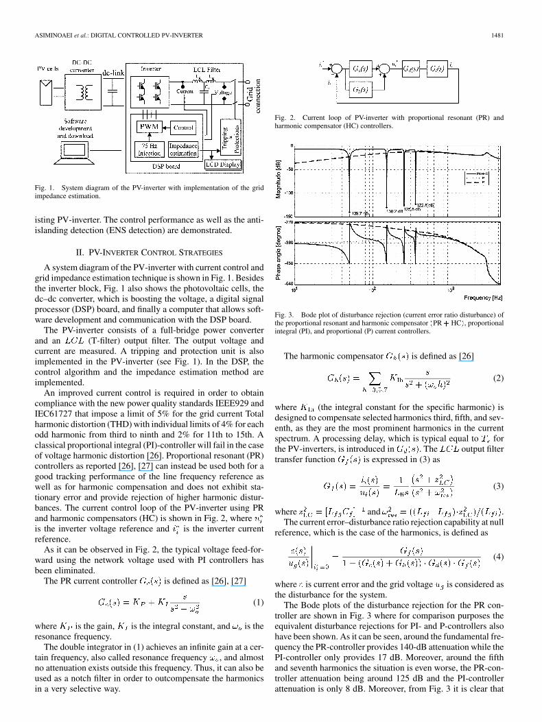
Fig. 1. System diagram of the PV-inverter with implementation of the gridimpedance estimation.

isting PV-inverter. The control performance as well as the anti-islanding detection (ENS detection) are demonstrated.

II. PV-INVERTER CONTROL STRATEGIES

A system diagram of the PV-inverter with current control andgrid impedance estimation technique is shown in Fig. 1. Besidesthe inverter block, Fig. 1 also shows the photovoltaic cells, thedc–dc converter, which is boosting the voltage, a digital signalprocessor (DSP) board, and finally a computer that allows soft-ware development and communication with the DSP board.

The PV-inverter consists of a full-bridge power converterand an (T-filter) output filter. The output voltage andcurrent are measured. A tripping and protection unit is alsoimplemented in the PV-inverter (see Fig. 1). In the DSP, thecontrol algorithm and the impedance estimation method areimplemented.

An improved current control is required in order to obtaincompliance with the new power quality standards IEEE929 andIEC61727 that impose a limit of 5% for the grid current Totalharmonic distortion (THD) with individual limits of 4% for eachodd harmonic from third to ninth and 2% for 11th to 15th. Aclassical proportional integral (PI)-controller will fail in the caseof voltage harmonic distortion [26]. Proportional resonant (PR)controllers as reported [26], [27] can instead be used both for agood tracking performance of the line frequency reference aswell as for harmonic compensation and does not exhibit sta-tionary error and provide rejection of higher harmonic distur-bances. The current control loop of the PV-inverter using PRand harmonic compensators (HC) is shown in Fig. 2, whereis the inverter voltage reference and is the inverter currentreference.

As it can be observed in Fig. 2, the typical voltage feed-for-ward using the network voltage used with PI controllers hasbeen eliminated.

The PR current controller is defined as [26], [27]

(1)

where is the gain, is the integral constant, and is theresonance frequency.

The double integrator in (1) achieves an infinite gain at a cer-tain frequency, also called resonance frequency , and almostno attenuation exists outside this frequency. Thus, it can also beused as a notch filter in order to outcompensate the harmonicsin a very selective way.

Fig. 2. Current loop of PV-inverter with proportional resonant (PR) andharmonic compensator (HC) controllers.

Fig. 3. Bode plot of disturbance rejection (current error ratio disturbance) ofthe proportional resonant and harmonic compensator (PR + HC), proportionalintegral (PI), and proportional (P) current controllers.

The harmonic compensator is defined as [26]

(2)

where (the integral constant for the specific harmonic) isdesigned to compensate selected harmonics third, fifth, and sev-enth, as they are the most prominent harmonics in the currentspectrum. A processing delay, which is typical equal to forthe PV-inverters, is introduced in . The output filtertransfer function is expressed in (3) as

(3)

where and .The current error–disturbance ratio rejection capability at null

reference, which is the case of the harmonics, is defined as

(4)

where is current error and the grid voltage is considered asthe disturbance for the system.

The Bode plots of the disturbance rejection for the PR con-troller are shown in Fig. 3 where for comparison purposes theequivalent disturbance rejections for PI- and P-controllers alsohave been shown. As it can be seen, around the fundamental fre-quency the PR-controller provides 140-dB attenuation while thePI-controller only provides 17 dB. Moreover, around the fifthand seventh harmonics the situation is even worse, the PR-con-troller attenuation being around 125 dB and the PI-controllerattenuation is only 8 dB. Moreover, from Fig. 3 it is clear that

1482 IEEE TRANSACTIONS ON POWER ELECTRONICS, VOL. 20, NO. 6, NOVEMBER 2005

the PI-controller rejection capability at the fifth and seventh har-monic is comparable with that of a simple proportional con-troller, the integral action being irrelevant.

Thus, the superiority of the PR-controller is demonstratedcompared to the PI-controller in terms of harmonic current re-jection.

The size of the proportional gain from the PR-controllerdetermines the bandwidth and phase margin stability, in thesame way as the classical PI-controller. A gain equal to2 leads to a bandwidth of about 650 Hz. This was consideredsatisfactory in respect to a used sampling frequency of 8.5 kHz.The phase margin (PM) is determined to be equal to 72 indi-cating a high stability. The integral constant acts to eliminatethe steady-state error [26]. Another aspect is that determinesthe bandwidth centered at the resonance frequency, which in thiscase is the grid frequency, where the attenuation is positive. Usu-ally, the grid frequency is stiff and is only allowed to vary in anarrow range, typically 1%. A value of 300 was deter-mined by simulations in order to eliminate the steady-state errorat the grid frequency.

Having the fundamental component current controller de-signed, the harmonic compensator is being added. In thiscase, the integral constant has the same effect as for thefundamental component, i.e., eliminating the steady-state error,just that the resonance frequencies are synchronous with thethird, fifth, and seventh harmonics. In this way, a selectiveharmonic compensation can be achieved without affecting thefundamental controller dynamics.

III. LINE IMPEDANCE MEASUREMENT TECHNIQUES

This section gives a survey of the commonly used methods forline impedance measurement. An extended work can be foundin [3] that describes in different general approaches for mea-suring the network harmonic impedance either in single- or inthree-phase systems, for low-, medium-, and high-voltage in-stallations. In this section, these methodologies are presentedin respect to the actual purpose of the work, i.e., PV-inverter.Therefore, as the methods are described hereafter, different lim-itations are shown and argued for the chosen method.

It is noticeable that the grid impedance measuring methodsare usually using dedicated hardware devices. Once the inputsignals are acquired by voltage and current measurement, theprocessing part follows, which typically involves large mathe-matical calculations in order to obtain the impedance value. [4]

Fig. 4 shows the usual technique for impedance measuring.The dedicated measuring device is denoted by “Z”-block andis normally a separated part of the inverter. , and arethe grid lumped resistance, capacitance, and inductance, whileV stands for the voltage supply. The “ ” argument shows themodel dependency on the harmonic order.

The state of the art [3] divides the measuring solutions intotwo major categories: passive and active methods.

Passive methods use the information about the noncharacter-istic harmonics voltages and currents that are already present inthe system. Therefore, as these methods depend on the existingbackground distortion of the voltage [3], [8] and, in many cases,the distortion does have either the amplitude or the repetitionrate to be properly measured, this turns out to be very difficultfor a PV implementation.

Fig. 4. Diagram of the PV-inverter connected to the grid. The grid impedanceis measured with an external device (Z).

Active methods make use of a provoked disturbance into thepower supply network followed by acquisition and signal pro-cessing. The way of “disturbing” the network can vary, thereforeactive methods are also divided into two major categories: tran-sient methods and steady-state methods.

A. Transient Active Methods

Transient methods are well suited for obtaining fast results,due to the short time of the disturbing effect on the network.Briefly, with this technique the device (“ ” in Fig. 4), generatesa transient current into the network (e.g., a resistive short-cir-cuit), and then measures the grid voltage and current at twodifferent time instants, before and after the impulse occurrence(short-circuit). The impulse will contain harmonics in a largespectrum. A similar approach is reported in [5] where the tran-sient is a damped oscillation created by connecting a known ca-pacitor. The results obtained give the network response over alarge frequency range, making such methods well suited in ap-plications where the impedance must be known at different fre-quencies. However, the methods must involve high performanceA/D acquisition devices and also must use special numericaltechniques to eliminate noise and random errors [12], [13].

These requirements are difficult to be achieved on a nonded-icated harmonic analyzer platform like a PV-inverter even if apowerful DSP is used, because the DSP already has specific andimportant tasks as mentioned in Section II.

B. Steady-State Active Methods

Steady-state methods typically inject a known and periodicaldistortion into the grid and then make the analysis in steady-state. One technique proposes the development of a dedicatedinverter topology [16] where the phase difference between thesupply voltage and the inverter voltage is measured and usedto calculate the line impedance. Another method uses the tech-nique of repetitively connecting a capacitive load to the networkand measuring the difference in phase shift between the voltageand current [17].

The technique used in this paper is also reported in [23] whichis a steady-state technique that injects an interharmonic currentinto the network and records the voltage change response. Theinput signals are processed by means of Fourier analysis at theparticular injected harmonic frequency. In this way, the methodhas the entire control of the injected current and the computa-tion needs only a few Fourier-terms for obtaining the final re-sult. As the pre-existing harmonics on the grid do not overlapon the frequency used for the interharmonic current injection,their effects are small, and this has the advantage of using lowsignal level for measurement [3]. This technique can be used to

ASIMINOAEI et al.: DIGITAL CONTROLLED PV-INVERTER 1483

obtain the frequency characteristic of the grid for a wide fre-quency range from 0 to 2.5 kHz [14]–[16] if the method repeatsthe measurements at different frequencies [10] followed by aninterpolation of the results. Such knowledge about the frequencycharacteristic of the grid is certainly useful for the PV-invertercontrol [6] and also for estimating the voltage distortion cre-ated by the PV-inverter current over the grid impedance [18].But an exact determination of the grid impedance over a widefrequency range will provide too many data than required forthe actual purpose, since the grid impedance must be known atthe fundamental frequency only. The method may not be veryprecise for the entire frequency range [10], as it depends on theinjecting signal levels, length and type of the windowing func-tion, selected sampling frequency, available resolution for theA/D converter, existing noise and disturbances on the grid, etc.However, as this method does not require any special hardwarebut still has control over the measurement process, it is very con-venient for a practical implementation in PV-inverters [7].

IV. PRINCIPLE OF OPERATION

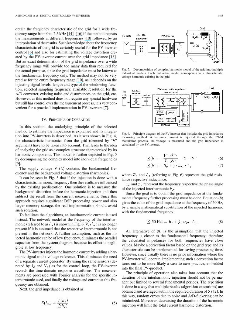
In this section, the underlying principle of the selectedmethod to estimate the impedance is explained and its integra-tion into PV-inverters is described. As it was shown in Fig. 4,the characteristic harmonics from the grid (denoted by “ ”argument) have to be taken into account. That leads to the ideaof analyzing the grid as a complex structure characterized by itsharmonic components. This model is further depicted in Fig. 5by decomposing the complex model into individual frequencies[9].

The supply voltage V contains the fundamental fre-quency and the background voltage distortion (harmonics).

It can be seen in Fig. 5 that if the injection is done with acharacteristic harmonic frequency then the results are influencedby the existing predistortion. One solution is to measure thebackground distortion before the harmonic injection and thensubtract the result from the current measurements. Since thisapproach requires significant DSP processing power and alsolarger memory storage, the real implementation should avoidsuch solution.

To facilitate the algorithms, an interharmonic current is usedinstead. The network model at the frequency of the interhar-monic (referred to as ) is shown in Fig. 6. V is no longerpresent if it is assumed that the respective interharmonic is notpresent in the network. A further assumption, such as the in-jected harmonic can be of low frequency, eliminates the parallelcapacitor from the system diagram because its effect is negli-gible at low frequency.

The PV-inverter injects the harmonic current by adding a har-monic signal to the voltage reference. This eliminates the needof a separate current generator. By using the same sensors (de-noted by and V ) as for the control loop, the PV-inverterrecords the time-domain response waveforms. The measure-ments are processed with Fourier analysis for the specific in-terharmonic used, and finally the voltage and current at this fre-quency are obtained.

Next, the grid impedance is obtained as

(5)

Fig. 5. Decomposition of complex harmonic model of the grid into multipleindividual models. Each individual model corresponds to a characteristicvoltage harmonic existing in the grid.

Fig. 6. Principle diagram of the PV-inverter that includes the grid impedancemeasuring method. A harmonic current is injected through the PWMmodulation process, the voltage is measured and the grid impedance iscalculated by the PV-inverter.

(6)

(7)

where and (referring to Fig. 6) represent the grid resis-tance respective inductance;

and represent the frequency respective the phase angleof the injected interharmonic .

Since the goal is to obtain the grid impedance at the funda-mental frequency further processing must be done. Equation (8)gives the value of the grid impedance at the frequency of 50 Hz,by a simple mathematical substitution of the injected harmonicwith the fundamental frequency

50 Hz (8)

An alternative of (8) is the assumption that the injectedfrequency is closer to the fundamental frequency; thereforethe calculated impedances for both frequencies have closevalues. Maybe a correction factor based on the grid type and itscharacteristic can be implemented for saving processing time.However, since usually there is no prior information where thePV-inverter will operate, implementing such a correction factorturns out to be more likely a case to case practice, embeddedinto the final PV-product.

The principle of operation also takes into account that theduration of the interharmonic injection should not be perma-nent but limited to several fundamental periods. The repetitionis done in a way that multiple results (algorithm executions) areobtained and averaged within the required duration of 5 s [2]. Inthis way, random errors due to noise and A/D-flickering can beminimized. Moreover, decreasing the duration of the harmonicinjection will limit the total current harmonic distortion.

1484 IEEE TRANSACTIONS ON POWER ELECTRONICS, VOL. 20, NO. 6, NOVEMBER 2005

Even this approach adds a certain degree of complexity. Ithas the advantage of allowing other similar PV-inverters (ex-ample: multiple inverters connected together in a PV farm) tooperate on (to measure) the same grid. Thus, the inverter makesthe injection, measures the effect, and then waits in an idle state.During this interval any other similar PV-inverter is allowed tomeasure the grid impedance without being disturbed.

As it can be seen, the underlying principle is relatively simpleand easy to be done with the PV-inverter, but there are differentissues that must be taken into account in a digital implementa-tion, which will be described in the next section.

V. IMPLEMENTATION

Regarding the implementation of the impedance measure-ment, there are two techniques of interest.

• A single-harmonic (SH) injection. When the grid ismeasured using a single interharmonic, then the resultsare translated from this frequency to the fundamentalaccording to (6)–(8).

• Two-harmonic (TH) injections. When the measurementprocess injects two interharmonics then the two discreteFourier transformation (DFT) results are interpolated togive the impedance at the fundamental frequency.

A. Single Harmonic (SH) Injection

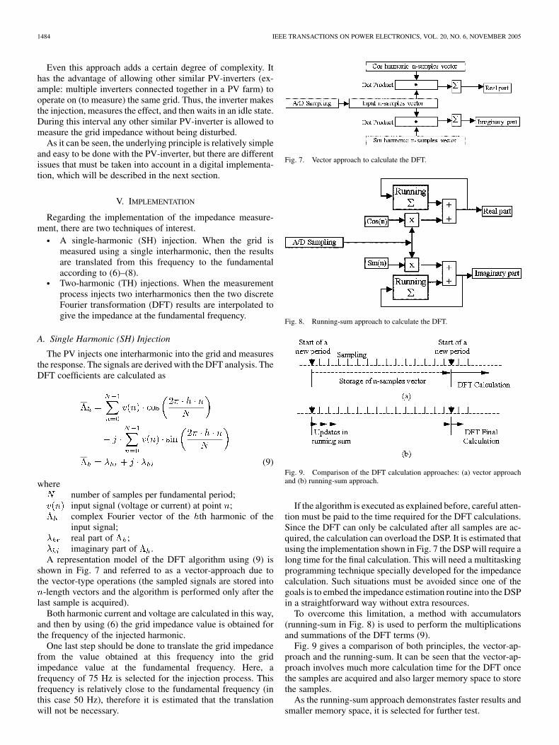
The PV injects one interharmonic into the grid and measuresthe response. The signals are derived with the DFT analysis. TheDFT coefficients are calculated as

(9)

wherenumber of samples per fundamental period;input signal (voltage or current) at point ;complex Fourier vector of the th harmonic of theinput signal;real part of ;imaginary part of .

A representation model of the DFT algorithm using (9) isshown in Fig. 7 and referred to as a vector-approach due tothe vector-type operations (the sampled signals are stored into

-length vectors and the algorithm is performed only after thelast sample is acquired).

Both harmonic current and voltage are calculated in this way,and then by using (6) the grid impedance value is obtained forthe frequency of the injected harmonic.

One last step should be done to translate the grid impedancefrom the value obtained at this frequency into the gridimpedance value at the fundamental frequency. Here, afrequency of 75 Hz is selected for the injection process. Thisfrequency is relatively close to the fundamental frequency (inthis case 50 Hz), therefore it is estimated that the translationwill not be necessary.

Fig. 7. Vector approach to calculate the DFT.

Fig. 8. Running-sum approach to calculate the DFT.

Fig. 9. Comparison of the DFT calculation approaches: (a) vector approachand (b) running-sum approach.

If the algorithm is executed as explained before, careful atten-tion must be paid to the time required for the DFT calculations.Since the DFT can only be calculated after all samples are ac-quired, the calculation can overload the DSP. It is estimated thatusing the implementation shown in Fig. 7 the DSP will require along time for the final calculation. This will need a multitaskingprogramming technique specially developed for the impedancecalculation. Such situations must be avoided since one of thegoals is to embed the impedance estimation routine into the DSPin a straightforward way without extra resources.

To overcome this limitation, a method with accumulators(running-sum in Fig. 8) is used to perform the multiplicationsand summations of the DFT terms (9).

Fig. 9 gives a comparison of both principles, the vector-ap-proach and the running-sum. It can be seen that the vector-ap-proach involves much more calculation time for the DFT oncethe samples are acquired and also larger memory space to storethe samples.

As the running-sum approach demonstrates faster results andsmaller memory space, it is selected for further test.

ASIMINOAEI et al.: DIGITAL CONTROLLED PV-INVERTER 1485

B. Two-Harmonic Injection

The TH injection consists of injecting two harmonics at thesame moment, then the DFT calculates the amplitude for thosetwo particular injected harmonics.

The TH injection is useful when both and need to becalculated. Thus, by having the grid impedance value at twodifferent frequencies, and are obtained from

(10)

(11)

(12)

whereinjected harmonic frequencies;impedances calculated at ;grid resistance and inductance.

Theoretically, this method gives the result of the gridimpedance (and in addition the grid resistance and inductance),but simulations and further studies have not validated thismethod to be the best for the PV-inverter. If the interval be-tween the chosen frequencies is too narrow then (11) and (12)can fall into numerical problems, especially with fixed-pointDSP because of a small denominator. On the opposite, if theinterval is larger, then the highest chosen frequency can be neara grid resonance point, which again gives a wrong estimationof the final result.

Thus, even if initially the TH method gains attention becauseof the advantage of obtaining the and values, the draw-backs mentioned, also encountered later in the simulation andexperimental phase, lean for the first method, the SH injection.

VI. SIMULATION OF THE IMPEDANCE DETECTION METHOD

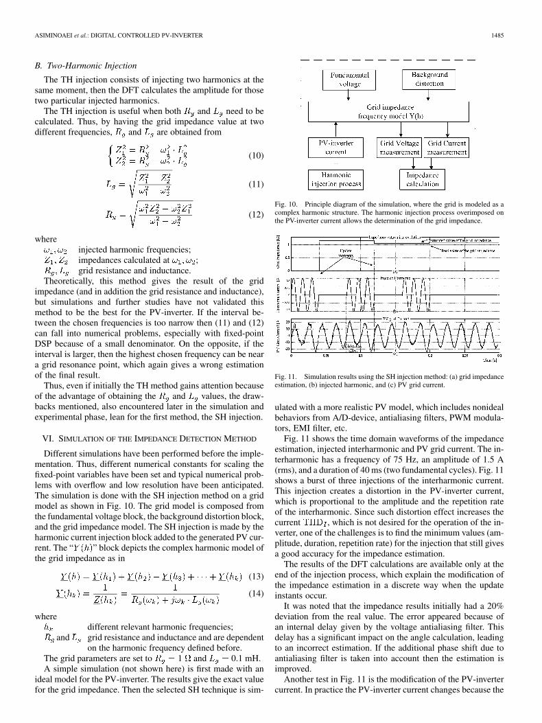
Different simulations have been performed before the imple-mentation. Thus, different numerical constants for scaling thefixed-point variables have been set and typical numerical prob-lems with overflow and low resolution have been anticipated.The simulation is done with the SH injection method on a gridmodel as shown in Fig. 10. The grid model is composed fromthe fundamental voltage block, the background distortion block,and the grid impedance model. The SH injection is made by theharmonic current injection block added to the generated PV cur-rent. The “ ” block depicts the complex harmonic model ofthe grid impedance as in

(13)

(14)

wheredifferent relevant harmonic frequencies;

and grid resistance and inductance and are dependenton the harmonic frequency defined before.

The grid parameters are set to 1 and 0.1 mH.A simple simulation (not shown here) is first made with an

ideal model for the PV-inverter. The results give the exact valuefor the grid impedance. Then the selected SH technique is sim-

Fig. 10. Principle diagram of the simulation, where the grid is modeled as acomplex harmonic structure. The harmonic injection process overimposed onthe PV-inverter current allows the determination of the grid impedance.

Fig. 11. Simulation results using the SH injection method: (a) grid impedanceestimation, (b) injected harmonic, and (c) PV grid current.

ulated with a more realistic PV model, which includes nonidealbehaviors from A/D-device, antialiasing filters, PWM modula-tors, EMI filter, etc.

Fig. 11 shows the time domain waveforms of the impedanceestimation, injected interharmonic and PV grid current. The in-terharmonic has a frequency of 75 Hz, an amplitude of 1.5 A(rms), and a duration of 40 ms (two fundamental cycles). Fig. 11shows a burst of three injections of the interharmonic current.This injection creates a distortion in the PV-inverter current,which is proportional to the amplitude and the repetition rateof the interharmonic. Since such distortion effect increases thecurrent , which is not desired for the operation of the in-verter, one of the challenges is to find the minimum values (am-plitude, duration, repetition rate) for the injection that still givesa good accuracy for the impedance estimation.

The results of the DFT calculations are available only at theend of the injection process, which explain the modification ofthe impedance estimation in a discrete way when the updateinstants occur.

It was noted that the impedance results initially had a 20%deviation from the real value. The error appeared because ofan internal delay given by the voltage antialiasing filter. Thisdelay has a significant impact on the angle calculation, leadingto an incorrect estimation. If the additional phase shift due toantialiasing filter is taken into account then the estimation isimproved.

Another test in Fig. 11 is the modification of the PV-invertercurrent. In practice the PV-inverter current changes because the

1486 IEEE TRANSACTIONS ON POWER ELECTRONICS, VOL. 20, NO. 6, NOVEMBER 2005

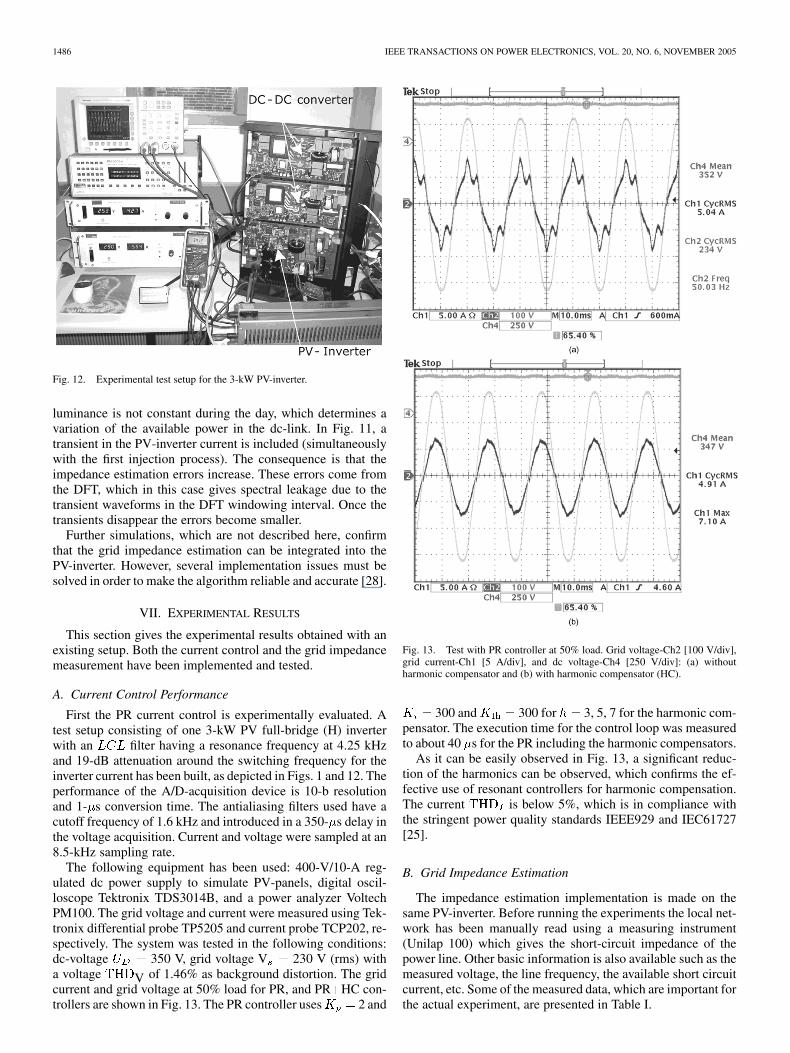
Fig. 12. Experimental test setup for the 3-kW PV-inverter.

luminance is not constant during the day, which determines avariation of the available power in the dc-link. In Fig. 11, atransient in the PV-inverter current is included (simultaneouslywith the first injection process). The consequence is that theimpedance estimation errors increase. These errors come fromthe DFT, which in this case gives spectral leakage due to thetransient waveforms in the DFT windowing interval. Once thetransients disappear the errors become smaller.

Further simulations, which are not described here, confirmthat the grid impedance estimation can be integrated into thePV-inverter. However, several implementation issues must besolved in order to make the algorithm reliable and accurate [28].

VII. EXPERIMENTAL RESULTS

This section gives the experimental results obtained with anexisting setup. Both the current control and the grid impedancemeasurement have been implemented and tested.

A. Current Control Performance

First the PR current control is experimentally evaluated. Atest setup consisting of one 3-kW PV full-bridge (H) inverterwith an filter having a resonance frequency at 4.25 kHzand 19-dB attenuation around the switching frequency for theinverter current has been built, as depicted in Figs. 1 and 12. Theperformance of the A/D-acquisition device is 10-b resolutionand 1- s conversion time. The antialiasing filters used have acutoff frequency of 1.6 kHz and introduced in a 350- s delay inthe voltage acquisition. Current and voltage were sampled at an8.5-kHz sampling rate.

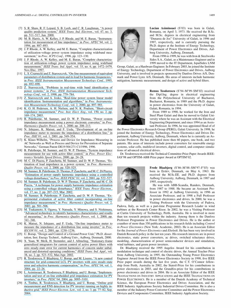
The following equipment has been used: 400-V/10-A reg-ulated dc power supply to simulate PV-panels, digital oscil-loscope Tektronix TDS3014B, and a power analyzer VoltechPM100. The grid voltage and current were measured using Tek-tronix differential probe TP5205 and current probe TCP202, re-spectively. The system was tested in the following conditions:dc-voltage 350 V, grid voltage V 230 V (rms) witha voltage V of 1.46% as background distortion. The gridcurrent and grid voltage at 50% load for PR, and PR HC con-trollers are shown in Fig. 13. The PR controller uses 2 and

Fig. 13. Test with PR controller at 50% load. Grid voltage-Ch2 [100 V/div],grid current-Ch1 [5 A/div], and dc voltage-Ch4 [250 V/div]: (a) withoutharmonic compensator and (b) with harmonic compensator (HC).

300 and 300 for 3, 5, 7 for the harmonic com-pensator. The execution time for the control loop was measuredto about 40 s for the PR including the harmonic compensators.

As it can be easily observed in Fig. 13, a significant reduc-tion of the harmonics can be observed, which confirms the ef-fective use of resonant controllers for harmonic compensation.The current is below 5%, which is in compliance withthe stringent power quality standards IEEE929 and IEC61727[25].

B. Grid Impedance Estimation

The impedance estimation implementation is made on thesame PV-inverter. Before running the experiments the local net-work has been manually read using a measuring instrument(Unilap 100) which gives the short-circuit impedance of thepower line. Other basic information is also available such as themeasured voltage, the line frequency, the available short circuitcurrent, etc. Some of the measured data, which are important forthe actual experiment, are presented in Table I.

ASIMINOAEI et al.: DIGITAL CONTROLLED PV-INVERTER 1487

TABLE IMANUAL MEASURED GRID PARAMETERS WITH UNILAP100 INSTRUMENT

TABLE IIMEASUREMENTS OF OUTPUT CURRENT AND BACKGROUND DISTORTION

WHEN THE PV POWER IS 3 kW

Fig. 14. Time-domain comparison of grid current with and without 1.5-Aharmonic injection. The PV power is 1.9 kW.

For measuring the grid quality, a power analyzer instrument(Voltech PM100) has been used to read the voltage and currentharmonics and their total distortion. The results are shown inTable II [27].

The interharmonic current injected has the frequency of75 Hz and an amplitude of 1.5 A. The injection process issynchronized with the fundamental frequency.

Fig. 14 shows the PV-inverter current for a power of 1.9 kWin two cases with and without the harmonic injection. The dif-ference is relatively small since the injected interharmonic hasa much smaller amplitude than the fundamental current.

The spectrum is displayed in Fig. 15 for both situations, withand without injection. The window duration is 40 ms (as shownin Fig. 14), which allows a correct FFT decomposition for the75 Hz and any multiple of the 50-Hz fundamental component.

As the injected interharmonic is not permanent, in real oper-ation the 75-Hz component is much smaller than presented inthis spectrum.

Fig. 15. Comparison of spectra with and without harmonic injection. (a) Gridvoltage. (b) Grid current (the signals in Fig. 14). The PV power is 3 kW.

Fig. 16. Method of the noncontinuous injection of the harmonic into the grid.Measured results with a repetition rate of two fundamental periods of injectionfrom a total of 13 fundamental periods (2/13).

The results show at 75 Hz that the harmonic voltage and cur-rent have amplitude values of 1.9 V respective 1.5 A. This givesa total grid impedance of 1.27 , at 75 Hz, which is relativelyclose to the value read in Table I.

Fig. 16 presents the PV grid current when the interharmonicinjection is performed with a repetition rate of 2/13 (two fun-damental cycles of interharmonic injection from a total of 13cycles).

This ratio was experimentally chosen based on a trade offbetween the losses due to the injection process and the accuracyof the measurement. If the repetition rate is too often then thepower used for the impedance measurement increases. On theother hand if the repetition rate is to rare then there are onlyfew measurements within the maximum time limit of 5 s, whichmight not be sufficient for an efficient filtering.

Table III gives such dependence on the repetition rate and theinterharmonic amplitude. The ratio of 2/13 was experimentallyconsidered as a good balance.

1488 IEEE TRANSACTIONS ON POWER ELECTRONICS, VOL. 20, NO. 6, NOVEMBER 2005

TABLE IIIEVALUATION OF IMPEDANCE MEASUREMENTS WITH DIFFERENT AMPLITUDES AND REPETITION RATES FOR A PV-INVERTER

POWER OF 1 kW. THE REAL GRID IMPEDANCE IS 1.2

Fig. 17. Impedance estimation when the PV current is changing from PVpower P = 0.3 kW to PV power P = 2 kW (scale factor is 1 V correspondingto 1 W). Here the harmonic injection process has a repetition rate of 2/13 andan amplitude of 1.3 A.

Further tests are performed (see Fig. 17) for assessing thestability of the result when the PV current changes. The PVcurrent is gradually increased by changing the internal currentreference in the PV-inverter, thus the power varies from 300 Wto 2 kW.

The internal calculation of the impedance is available forreading on a PWM analogue output from the DSP, filtered witha low pass RC-filter. This explains the high-frequency ripple onthe presented impedance waveform; hence one should read itsaverage value. The scale setting for displaying the impedance is1 V, which corresponds to 1 .

The experiments show that the impedance estimation is fairlystable as the PV current is changing. However, Slight variationsaround the mean value are noticed. For that reason, a post-pro-cessing phase is required to eliminate random errors and A/Dflickering. A practical way is to use a low-pass or a moving av-erage numerical filter.

Implementing an average filter over a period of 3 s gives 15%error in the grid impedance estimation, which is satisfactory forthe ENS requirements [29].

Since the result of the measurement is used to detect a stepchange of 0.5 in the grid impedance, the accuracy was nota prime factor in deciding the final implementation. Even if a

good accuracy is generally desired for any measuring equip-ment, however, other topics are also important in this case (theamplitude of the injection, repetition rate, created distortion,consumed power, synchronization with the fundamental, fil-tering and post-processing, detection speed, etc.) [28], [29].

VIII. CONCLUSION

This paper describes a digital implemented PV-inverter ap-plication with an advanced PR-controller for current trackingand an on-line method for grid impedance estimation. The mainfocus has been on using a steady-state intrusive method forthe grid impedance estimation as well as having a good cur-rent . Injecting an interharmonic current into the grid andmeasuring the voltage response can be used to estimate the gridimpedance.

In a context of practical use into a PV-inverter, this methodhas the advantages of low cost and easy implementation withthe existing hardware.

The paper reveals also the issues of implementing the pro-posed method into a DSP program. Finally, the approach ofmeasuring the grid impedance is validated by real measurementsand it works with an accuracy better than 15% and a current

of less than 5%.

REFERENCES

[1] F. Blaabjerg, Z. Chen, and S. B. Kjaer, “Power electronics as efficientinterface in dispersed power generation systems,” IEEE Trans. PowerElectron., vol. 19, no. 5, pp. 1184–1194, Sep. 2004.

[2] Photovoltaic Semiconductor Converters Part 1: Utility Interactive FailSafe Protective Interface for PV-Line Commutated Converters—DesignQualification and Type Approval, European Std. EN 50330-1, 1999.

[3] A. Robert, T. Deflandre, E. Gunther, R. Bergeron, A. Emanuel, A. Fer-rante, G. S. Finlay, R. Gretsch, A. Guarini, J. L. G. Iglesias, D. Hartmann,M. Lahtinen, R. Marshall, K. Oonishi, C. Pincella, S. Poulsen, P. Ribeiro,M. Samotyj, K. Sand, J. Smid, P. Wright, and Y. S. Zhelesko, “Guide forassessing the network harmonic impedance,” Proc. Inst. Elect. Eng., vol.2, pp. 301–310, 1997.

[4] A. de Oliveira, J. C. de Oliveira, J. W. Resende, and M. S.Miskulin, “Practical approaches for AC system harmonic impedancemeasurements,” Trans. Power Del., vol. 6, no. 4, pp. 1721–1726,Nov. 1991.

[5] W. C. Beatti and S. R. Matthews, “Impedance measurement on distribu-tion networks,” in Proc. Universities Power Engineering Conf., vol. 1,1994, pp. 117–120.

[6] M. Liserre, R. Teodorescu, and F. Blaabjerg, “Stability of grid-con-nected PV inverters with large grid impedance variation,” in Proc. IEEEPESC’04, 2004, pp. 4773–4779.

ASIMINOAEI et al.: DIGITAL CONTROLLED PV-INVERTER 1489

[7] S. R. Shaw, R. F. Lepard, S. B. Leeb, and C. R. Laughman, “A powerquality prediction system,” IEEE Trans. Ind. Electron., vol. 47, no. 3,pp. 511–517, Jun. 2000.

[8] M. B. Harris, A. W. Kelley, J. P. Rhode, and M. E. Baran, “Instrumen-tation for measurement of line impedance,” in Proc. APEC’94, vol. 2,1994, pp. 887–893.

[9] J. P. Rhode, A. W. Kelley, and M. E. Baran, “Complete characterizationof utilization-voltage power system impedance using wideband mea-surement,” in Proc. ICPS Conf., 1996, pp. 123–130.

[10] J. P. Rhode, A. W. Kelley, and M. E. Baran, “Complete characteriza-tion of utilization-voltage power system impedance using widebandmeasurement,” IEEE Trans. Ind. Appl., vol. 33, no. 6, pp. 1472–1479,Nov./Dec. 1997.

[11] L. S. Czarnecki and Z. Staroszczyk, “On-line measurement of equivalentparameters of distribution system and its load for harmonic frequencies,”in Proc. IEEE Instrumentation Measurement Technology Conf., 1995,pp. 692–698.

[12] Z. Staroszczyk, “Problems in real-time wide band identification ofpower systems,” in Proc. IEEE Instrumentation Measurement Tech-nology Conf., vol. 2, 1998, pp. 779–784.

[13] Z. Staroszczyk and A. Josko, “Real-time power system linear modelidentification: Instrumentation and algorithms,” in Proc. Instrumenta-tion Measurement Technology Conf., vol. 2, 2000, pp. 897–901.

[14] K. O. H. Pedersen, A. H. Nielsen, and N. K. Poulsen, “Short-circuitimpedance measurement,” Proc. Inst. Elect. Eng., vol. 150, no. 2, pp.169–174, 2003.

[15] B. Palethorpe, M. Sumner, and D. W. P. Thomas, “Power systemimpedance measurement using a power electronic converter,” in Proc.Harmonics Quality Power, vol. 1, 2000, pp. 208–213.

[16] N. Ishigure, K. Matsui, and F. Ueda, “Development of an on-lineimpedance meter to measure the impedance of a distribution line,” inProc. ISIE’01, vol. 1, 2001, pp. 549–554.

[17] K. Klaus-Wilhelm, “Process and Device for Impedance Measuring inAC Networks as Well as Process and Device for Prevention of SeparateNetworks,” German Patent DE19 504 271 C1/1996, 1996.

[18] B. Palethorpe, M. Sumner, and D. W. P. Thomas, “System impedancemeasurement for use with active filter control,” in Proc. Power Elec-tronics Variable Speed Drives, 2000, pp. 24–28.

[19] M. C. Di Piazza, P. Zanchetta, M. Sumner, and D. W. P. Thomas, “Es-timation of load impedance in a power system,” in Proc. HarmonicsQuality Power, vol. 2, 2000, pp. 520–525.

[20] M. Sumner, B. Palethorpe, D. Thomas, P. Zanchetta, and M. C. Di Piazza,“Estimation of power supply harmonic impedance using a controlledvoltage disturbance,” in Proc. IEEE PESC’01, vol. 2, 2001, pp. 522–527.

[21] M. Sumner, B. Palethorpe, D. W. P. Thomas, P. Zanchetta, and M. C. DiPiazza, “A technique for power supply harmonic impedance estimationusing a controlled voltage disturbance,” IEEE Trans. Power Electron.,vol. 17, no. 2, pp. 207–215, Mar. 2002.

[22] M. Sumner, B. Palethorpe, P. Zanchetta, and D. W. P. Thomas, “Ex-perimental evaluation of active filter control incorporating on-lineimpedance measurement,” in Proc. Harmonics Quality Power, vol. 2,2002, pp. 501–506.

[23] M. Tsukamoto, S. Ogawa, Y. Natsuda, Y. Minowa, and S. Nishimura,“Advanced technology to identify harmonics characteristics and resultsof measuring,” in Proc. Harmonics Quality Power, vol. 1, 2000, pp.341–346.

[24] K. Matsui, N. Ishigure, and F. Ueda, “On-line impedance meter tomeasure the impedance of a distribution line using inverter,” in Proc.IECON’01, vol. 2, 2001, pp. 1230–1236.

[25] U. Borup, “Design and Control of a Ground Power Unit,” Ph.D. disser-tation, Inst. Energy Technol., Aalborg Univ., Aalborg, Denmark, 2000.

[26] X. Yuan, W. Merk, H. Stemmler, and J. Allmeling, “Stationary-framegeneralized integrators for current control of active power filters withzero steady-state error for current harmonics of concern under unbal-anced and distorted operating conditions,” IEEE Trans. Ind. Appl., vol.38, no. 2, pp. 523–532, Mar./Apr. 2002.

[27] R. Teodorescu, F. Blaabjerg, U. Borup, and M. Liserre, “A new controlstructure for grid-connected LCL PV inverters with zero steady-stateerror and selective harmonic compensation,” in Proc. APEC’04, vol. 1,2004, pp. 22–26.

[28] L. Asiminoaei, R. Teodorescu, F. Blaabjerg, and U. Borup, “Implemen-tation and test of on-line embedded grid impedance estimation for PVinverters,” in Proc. PESC’04, 2004, pp. 3095–3101.

[29] A. Timbus, R. Teodorescu, F. Blaabjerg, and U. Borup, “Online gridmeasurement and ENS detection for PV inverter running on highly in-ductive grid,” IEEE Power Electron. Lett., vol. 2, no. 3, pp. 77–82, Sep.2004.

Lucian Asiminoaei (S’03) was born in Galati,Romania, on April 3, 1973. He received the B.Sc.and M.Sc. degrees in electrical engineering from“Dunarea de Jos” University of Galati, in 1996 and1997, respectively, and is currently pursuing thePh.D. degree at the Institute of Energy Technology,Department of Power Electronics and Drives, Aal-borg University, Aalborg, Denmark.

From 1996 to 1999, he was with Iron & SteelworksSidex S.A., Galati, as a Maintenance Engineer and in1999 moved to the IT Department, IspatSidex LNM

Group, Galati, as a Hardware Engineer. In February 2003, he joined the Instituteof Energy Technology, Department of Power Electronics and Drives, AalborgUniversity, and is involved in projects sponsored by Danfoss Drives A/S, Den-mark and Power Lynx A/S, Denmark. His areas of interests include harmonicmitigation, harmonic measurement, and design of active and hybrid filters.

Remus Teodorescu (S’94–M’99–SM’02) receivedthe Dipl.Ing. degree in electrical engineeringfrom the Polytechnical University of Bucharest,Bucharest, Romania, in 1989 and the Ph.D. degreein power electronics from the University of Galati,Galati, Romania, in 1994.

From 1989 to 1990, he worked for the Iron andSteel Plant Galati and then he moved to Galati Uni-versity where he was an Assistant with the ElectricalEngineering Department, and since 1994 as an Assis-tant Professor. In 1996, he was appointed Head of of

the Power Electronics Research Group (PERG), Galati University. In 1998, hejoined the Institute of Energy Technology, Power Electronics and Drives De-partment, Aalborg University, Aalborg, Denmark, where he is currently an As-sociate Professor. He has published more then 60 papers, one book, and twopatents. His areas of interests include power converters for renewable energysystems, solar cells, multilevel inverters, digital control, and computer simula-tions of advanced electrical drives.

Dr. Teodorescu received the Technical Committee Prize Paper Awards IEEE-IAS’98 and OPTIM-ABB Prize paper Award at OPTIM’02.

Frede Blaabjerg (S’86–M’88–SM’97–F’03) wasborn in Erslev, Denmark, on May 6, 1963. Hereceived the M.Sc.EE. and Ph.D. degrees fromAalborg University, Aalborg, Denmark, in 1987 and1995, respectively.

He was with ABB-Scandia, Randers, Denmark,from 1987 to 1988. He became an Assistant Pro-fessor in 1992 at Aalborg University, in 1996 anAssociate Professor, and in 1998 a Full Professorin power electronics and drives. In 2000, he was aVisiting Professor with the University of Padova,

Padova, Italy, as well as a part-time Programme Research Leader in windturbines at the Research Center Risoe. In 2002, he was a Visiting Professorat Curtin University of Technology, Perth, Australia. He is involved in morethan ten research projects within the industry. Among them is the DanfossProfessor Programme in Power Electronics and Drives. He is the author orcoauthor of more than 350 publications in his research fields including Controlin Power Electronics (New York: Academic, 2002). He is an Associate Editorfor the Journal of Power Electronics and Elteknik. He has been very involved inDanish Research policy in the last ten years. His research interests are in powerelectronics, static power converters, ac drives, switched reluctance drives,modeling, characterization of power semiconductor devices and simulation,wind turbines, and green power inverters.

Dr. Blaabjerg received the 1995 Angelos Award for his contribution inmodulation technique and control of electric drives, the Annual Teacher Prizefrom Aalborg University, in 1995, the Outstanding Young Power ElectronicsEngineer Award from the IEEE Power Electronics Society in 1998, five IEEEPrize paper awards during the last five years, the C.Y. O’Connor fellow-ship from Perth, Australia in 2002, the Statoil-Prize for his contributions inpower electronics in 2003, and the Grundfos-prize for his contributions inpower electronics and drives in 2004. He is an Associate Editor of the IEEETRANSACTIONS ON INDUSTRY APPLICATIONS and the IEEE TRANSACTIONS ON

POWER ELECTRONICS. He is a member of the Danish Academy of TechnicalScience, the European Power Electronics and Drives Association, and theIEEE Industry Applications Society Industrial Drives Committee. He is also amember of the Industry Power Converter Committee and the Power ElectronicsDevices and Components Committee, IEEE Industry Application Society.

1490 IEEE TRANSACTIONS ON POWER ELECTRONICS, VOL. 20, NO. 6, NOVEMBER 2005

Uffe Borup (S’94–M’96) received the M.S.E.E. andPh.D. degrees in electrical engineering from AalborgUniversity, Aalborg, Denmark, in 1996 and 2000, re-spectively.

In 1996, he joined the Institute of Energy Tech-nology, Aalborg University, as a Research Assistant.During this period, he carried out a research projecton modeling of power semiconductors in the hor-izontal deflection circuit on television receivers(supported by the Danish television producer Bang& Olufsen A/S). In August 1997, he joined AXA

Power, Odense, Denmark, as an industrial Ph.D. student on the project “Designand Control of a Ground Power Unit.” From 2000 to 2002, he was R&DProject Manager with AXA Power. In 2002, he cofounded PowerLynx A/S,Sønderborg, Denmark (a company that is developing PV-inverters) where he isthe Development Manager. He has authored more than 20 publications and hastwo patents pending. His primary research interests are advance converters forpower supplies and drives, including topology, control, harmonics, modeling,characterization of power semiconductor devices, and simulation.