EPS-meteograms ENS-meteograms - UiO

EPS-meteogramsENS-meteograms

EPS=Ensemble Prediction SystemENS=Ensemble (new name at ECMWF)

16.01.2016 00utc ana + 18.01.2016 00utc ana +

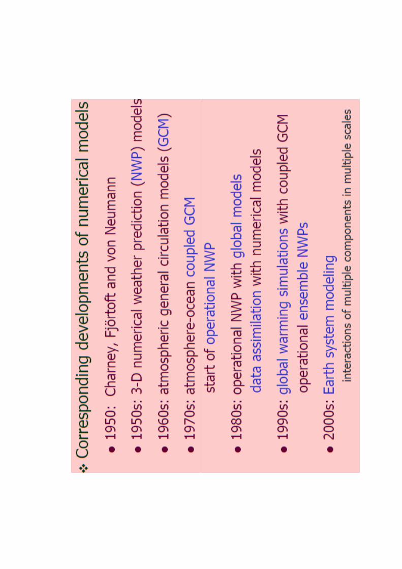
NWP Historics

Vilhelm F. K. Bjerknes (1904)

Founded the basis for WP as an exact science:

Classical fluid dynamics

+ classical thermodynamics

= “Physical fluid dynamics”= “Physical fluid dynamics”

Number of unknowns = number of equations.

PDE: Only first order in time

Exact Science Paradigm in 1904:

Observe at t=0 �Calculate every variable at any time t.

Determinism IN PRINCIPLE!Meteorologisk institutt met.no

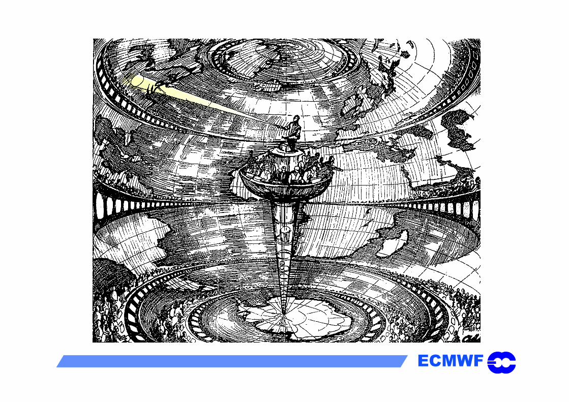
Lewis Fry Richardson (1881-1953)

The first numerical weather forecast –manual (!)

ECMWF

manual (!)

Meteorological «noise» and Richardson’s failure

The world’s first successful, purely calculated weather forecastInstitute of Advanced Study, Princeton Univ., USA,1946�1950

Arnt EliassenRagnar FjørtoftJule CharneyJohn von Neuman

ENIACThe computer

Fjørtoft

Z_500 t=0, analysis t=+24h, verifying analysis

∆Z, ana t=+24h, prognosis

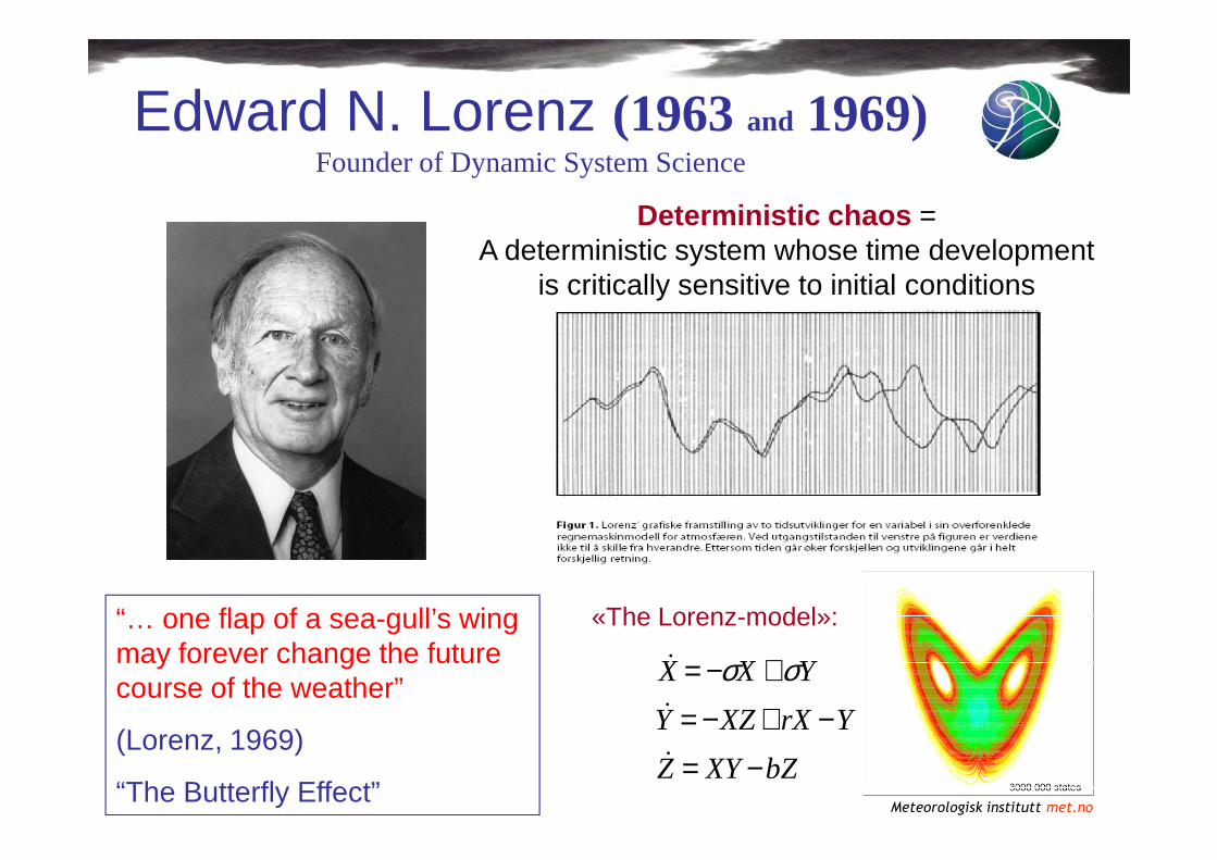
Edward N. Lorenz (1963 and 1969)Founder of Dynamic System Science

Deterministic chaos = A deterministic system whose time development

is critically sensitive to initial conditions

bZXYZ

YrXXZY

YXX

−=−+−=

+−=

&

&

& σσ

“… one flap of a sea-gull’s wing may forever change the future course of the weather”

(Lorenz, 1969)

“The Butterfly Effect”Meteorologisk institutt met.no

«The Lorenz-model»:

The Lorenz (1963) attractor, the prototype chaotic model…..

Development of the

S1-scores for Z500hPa and MSLPFor different forecast lengths

S1=70% =>useless forecastS1=20%=>perfect forecast

Development if RMS error of predicted geop. Height of 500 hPa

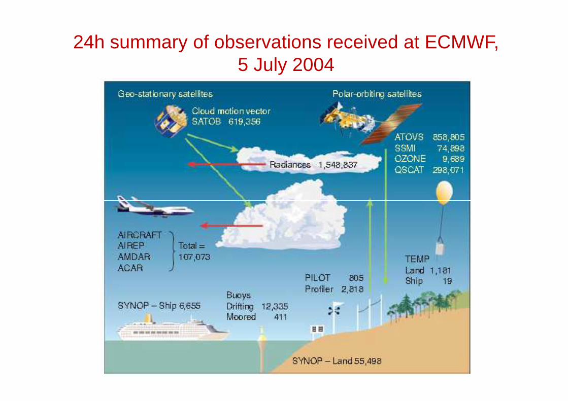
24h summary of observations received at ECMWF, 5 July 2004

RMSE and Anomaly correlation

= 0

Assuming:

Assume

Or:

Ej2 = 2Aa

2 (1 – ACj )

E=RMS Error AC=Anomaly Correlation

Ej2 = 2Aa

2 (1 – ACj )

Evolution of ECMWF scores over NH and SH for Z500

The combination of improved data-assimilation and forecasting models, the availability of more/better observations (especially from satellites), and higher computer power have led to increasingly accurate weather forecasts. Today, over NH (SH) a day-7 single forecast of the upper-air atmospheric flow has the same accuracy as a day-5 in 1985 (day-3 in 1981).

EC/TC/PR/RB-L1 2010 – Roberto Buizza: Sources of uncertainty23

Evolution of ECMWF scores over NH and SH for Z500 II

~210km ~16km

Quality of numerical model forecasts for the geopotential height of 500 hPa

Anomaly-correlation for forecasted Z(500hPa) from ECMWF’soperational, global modelsnce 1980

Courtesy: P.Kållberg, A. Simmons; ECMWF

Same results if the same («frozen»)model- and analysis-systemis used for all years(here: ECMWF’s re-analysis, «ERA»):

Changes are only due to-Random fluctuations (internal variability)-observational changes

Re-analyses & Re-forecasts in NWP verification

Z500 : Forecast time when ACC=80% N hemisphere

Operational (variations due to: weather, model, DA, and obs)

ERA Interim Re-forecasts (variations: weather and obs)

FD/RD September 2014Slide 26

Z500 N hemisphere Difference: Operational - ERA-Interim

Improved predictions over since 2000due to system improvements (and observation changes)

FD/RD September 2014Slide 27

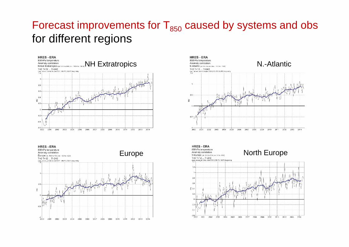
Forecast improvements for T850 caused by systems and obsfor different regions

NH Extratropics N.-Atlantic

Europe North Europe

Upward Trend in EPS (now: ENS)

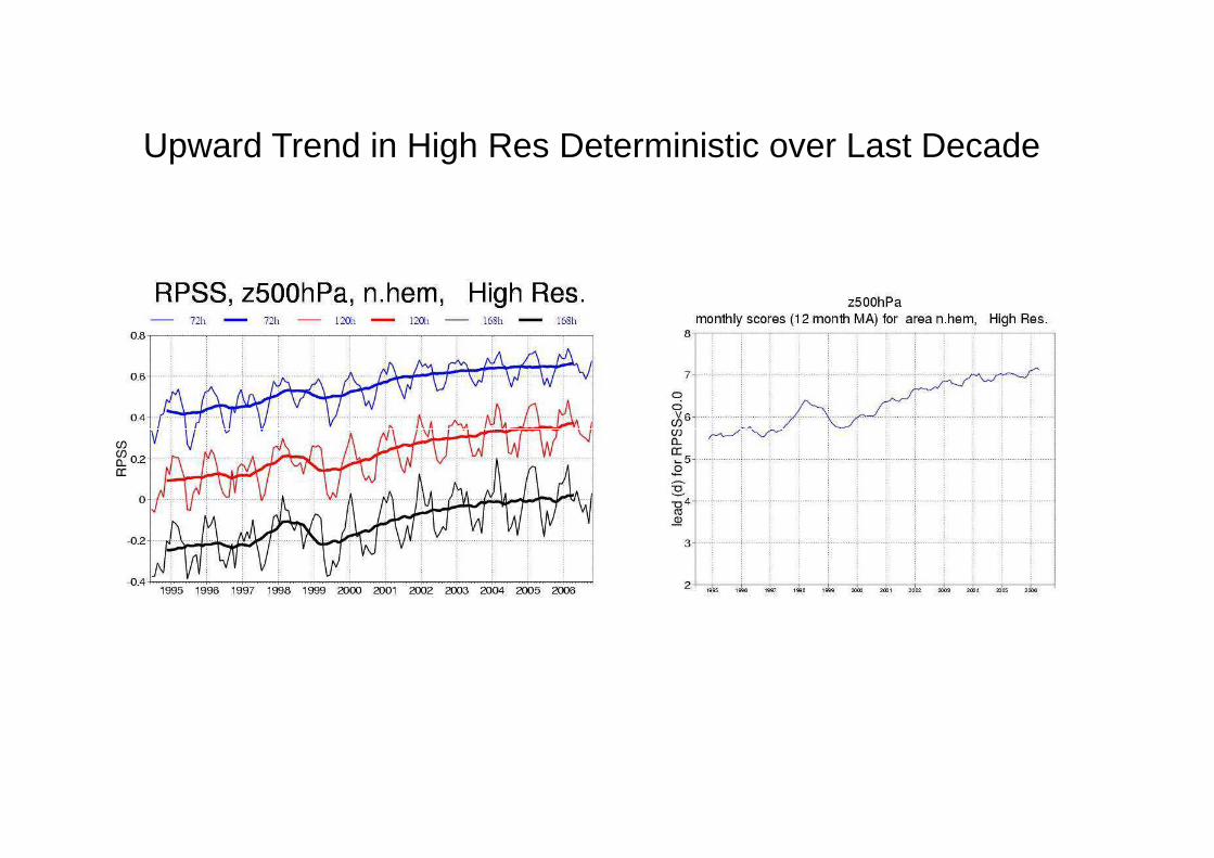
Upward Trend in High Res Deterministic over Last Decade

Simple mathematical systems possessing chaos

Logistic map

Lorenz «Butterfly»

Xn(r) when n�∝

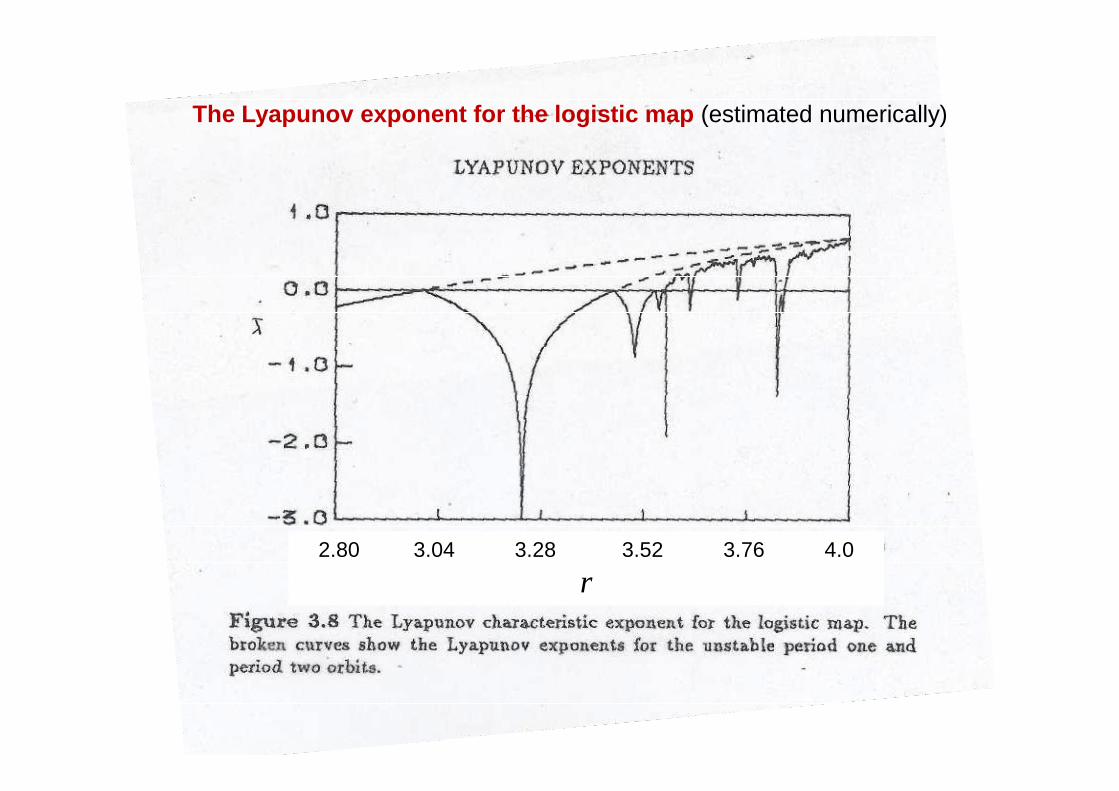
The Lyapunov exponent for the logistic map (estimated numerically)

2.80 3.04 3.28 3.52 3.76 4.0

r

Chaos Theory concepts

Kalnay Ch 6.2-6.3

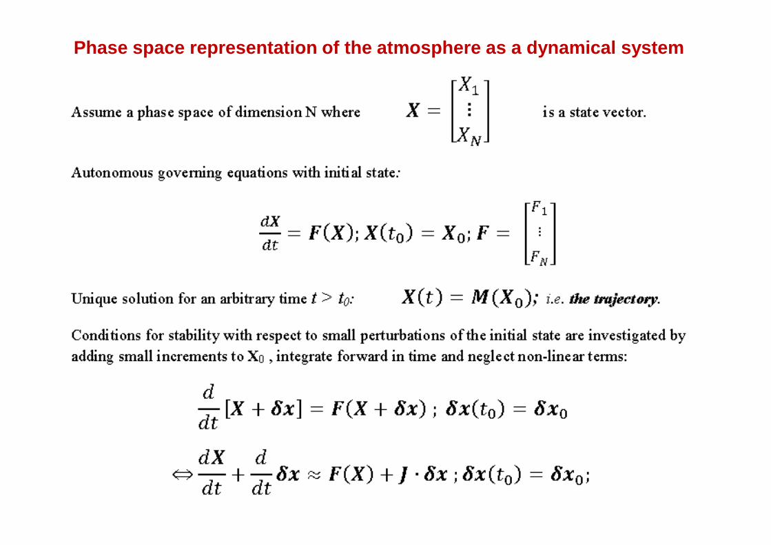
Phase space representation of the atmosphere as a dynamic al system

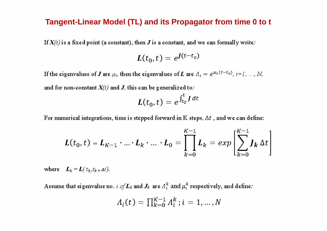
Tangent-Linear Model (TL) and its Propagator from tim e 0 to t

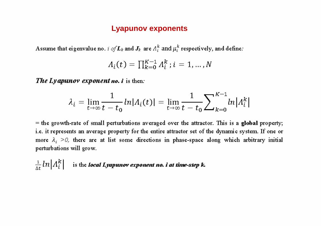
Lyapunov exponents

LOCAL LYAPUNOV VECTORS

the leading local Lyapunov exponent (i.e. no. 1):

.

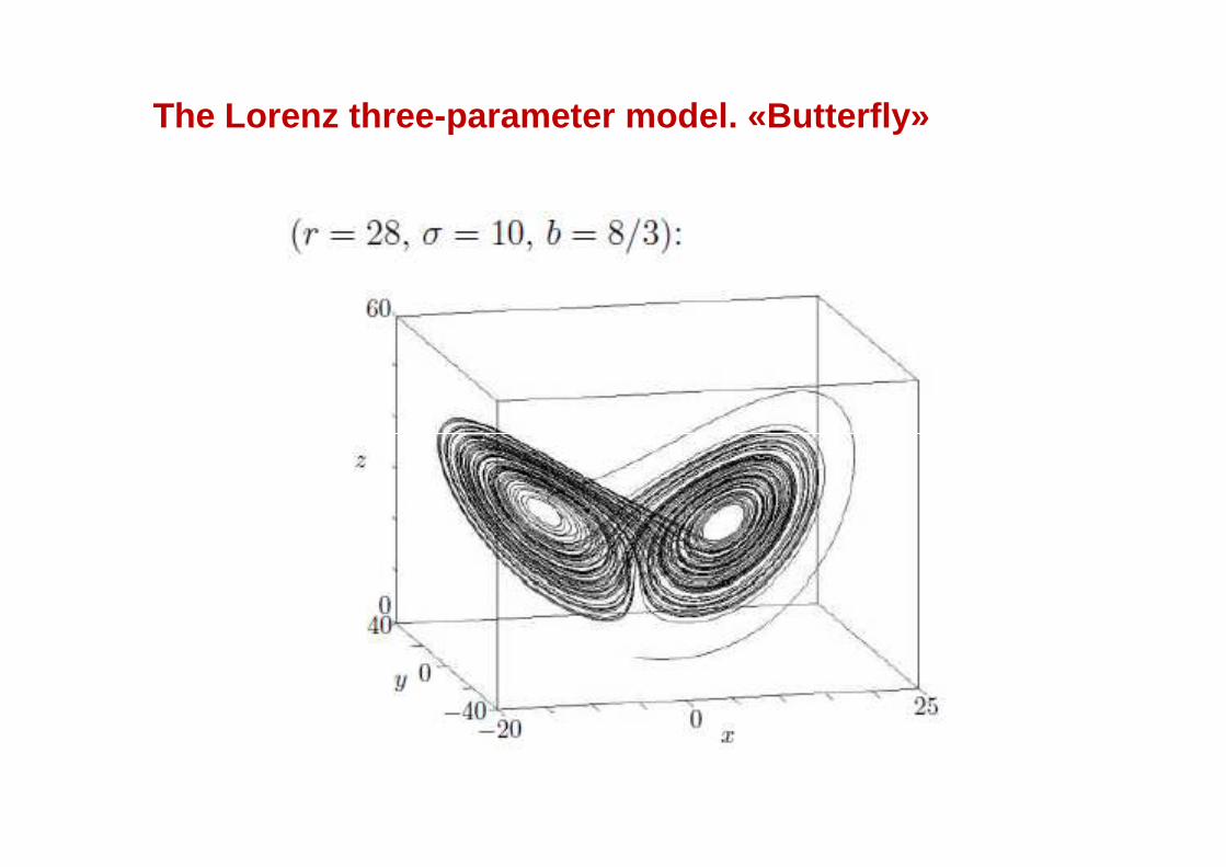
The Lorenz three-parameter model. «Butterfly»

The growth of perturbations: linear – weakly non-linear – strongly non-linear

Why probabilistic weather prediction?

Why not categorical («deterministic») forecasts

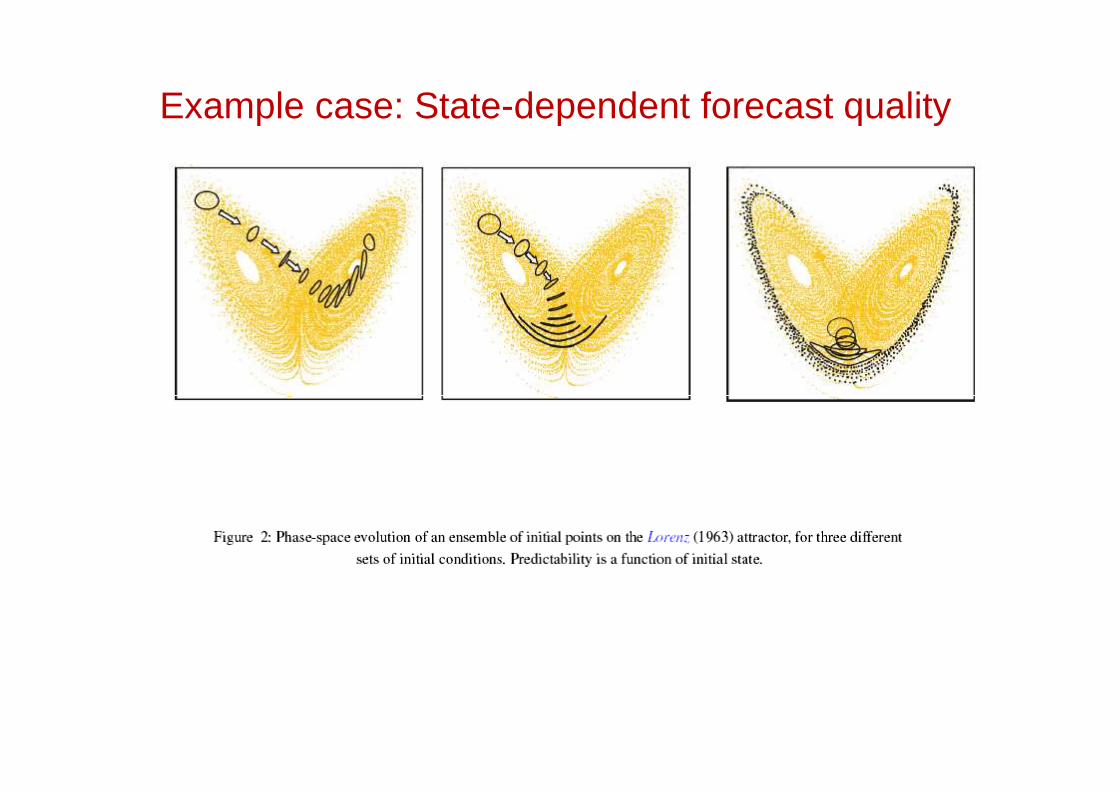
Example case: State-dependent forecast quality

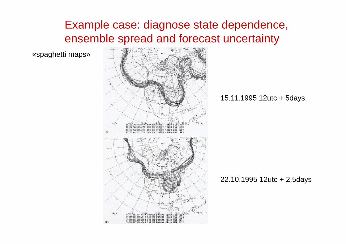
Example case: diagnose state dependence, ensemble spread and forecast uncertainty

«plumes»

For London UK

26.06.1995 00utc

26.06.1994 00utc

Example case: diagnose state dependence, ensemble spread and forecast uncertainty

«spaghetti maps»

15.11.1995 12utc + 5days

22.10.1995 12utc + 2.5days

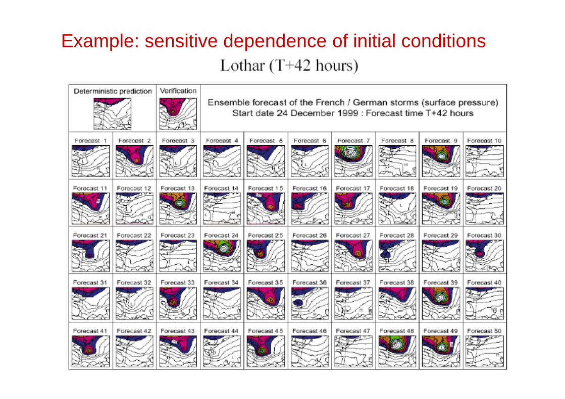
Example: sensitive dependence of initial conditions

But: Deterministic forecasts for 1-2 days are nearl y perfect ! - for z500

Courtesy: A. Simmons; ECMWF

NWP quality for 500hPa geopotential heights

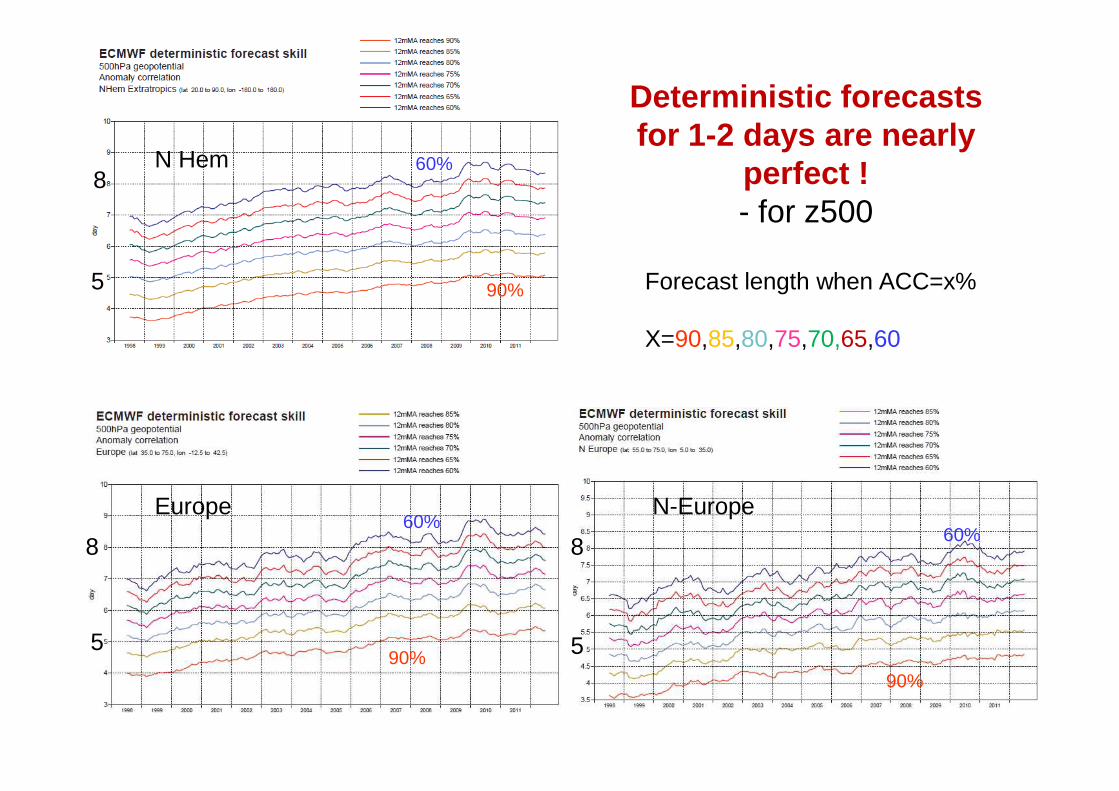
Deterministic forecasts for 1-2 days are nearly

perfect ! - for z500

N Hem

Forecast length when ACC=x%

X=90,85,80,75,70,65,60

5

8

90%

60%

Europe N-Europe

5 5

8 8

90%90%

60%60%

Brier Skill Score for 96h ECMWF EPS for selected events

ff10m against analysis

ECMWF operational verification

24hPrecip against analysis

24hPrecip against obsff10m against obs

ff10m against analysis

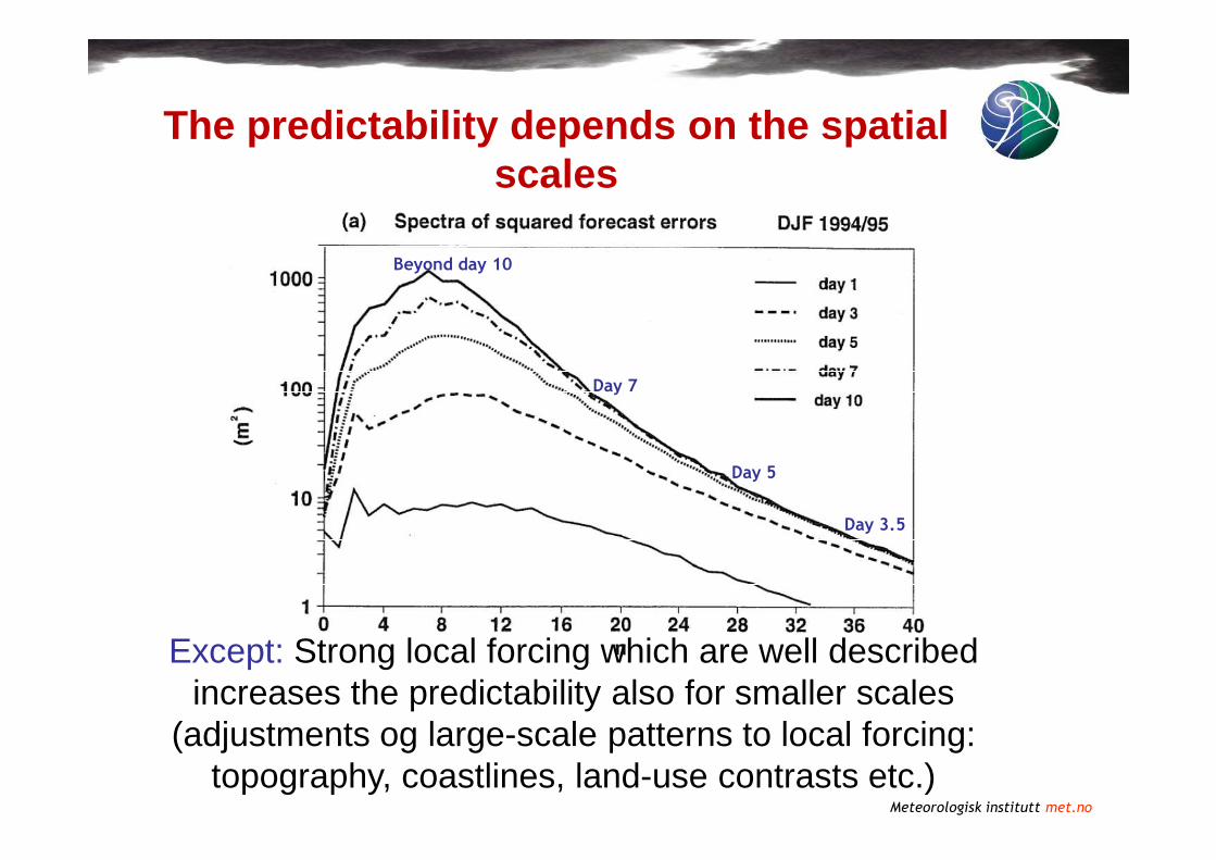
The predictability depends on the spatial scales

Day 7

Beyond day 10

Meteorologisk institutt met.no

Except: Strong local forcing which are well described increases the predictability also for smaller scales

(adjustments og large-scale patterns to local forcing: topography, coastlines, land-use contrasts etc.)

Day 3.5

Day 5

Predictability as a function of the spatial extension of weather systems


Forecast lead time when Rank Probability Skill Score (RPSS) for EC EPS of Z500 < 0.3

All scales Planetary scales

EPS

ctrldeterministic

Predictability as a function of the spatial extension of weather systems II

All scales Planetary scales

Synoptic scales

Sub-synoptic scales

Predictability as a function of the spatial extension of weather systems III


The consensus forecast:Unpredictable components are filtered

Winter1997-98

”Regression towards the mean”: when error-growth is non-linear, a majority of forecasts will

tend towards maximum climatological occurrence

In any case: to forecast extreme weather events categorically (either 100% or 0% certain) is overly

optimistic.

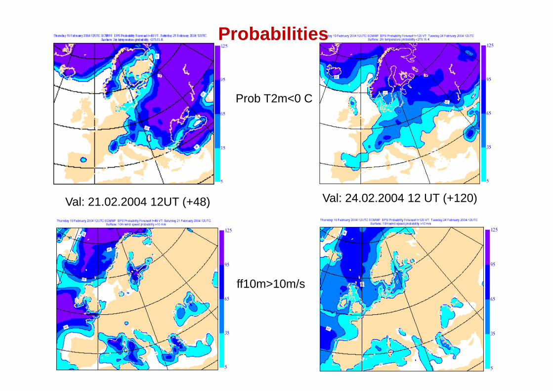
Prob T2m<0 C

Val: 21.02.2004 12UT (+48) Val: 24.02.2004 12 UT (+120)

Probabilities

Val: 21.02.2004 12UT (+48) Val: 24.02.2004 12 UT (+120)

ff10m>10m/s

Prob P>5 mm/24h

Val: 20.02.1995 12utc - 21.02.1995 12utc (+24 -48) Val: Tuesday 24.02.2004 0 -24utc (+108 -132)

Probabilities

Val: 20.02.1995 12utc - 21.02.1995 12utc (+24 -48) Val: Tuesday 24.02.2004 0 -24utc (+108 -132)

Prob P>10 mm/24h

Distances in phase-space, inner products, and the adjo int

Properties of the the adjoint

Singular Vectors, SVs


u1

The Lorenz modelSingular Values

Singular Vectors, SVs,

Examples

Singular Vectors, SVs, Examples

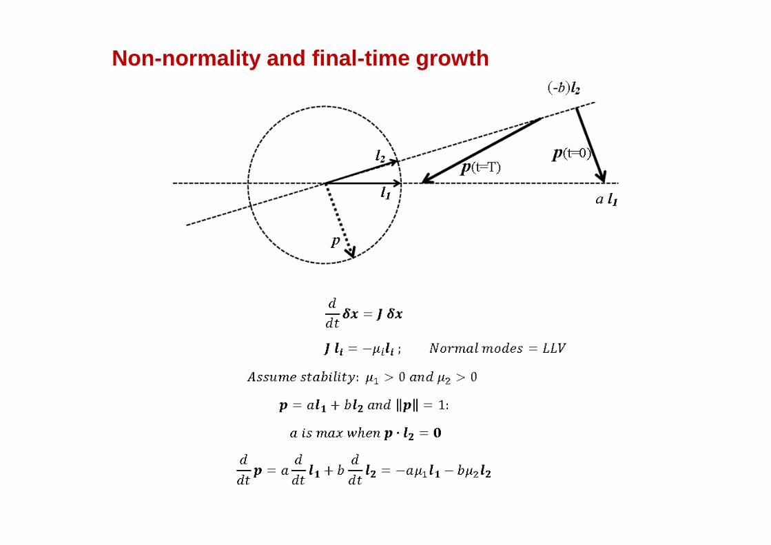
Non-normality and final-time growth

Initial perturbations

Operational ensemble prediction

Predictability varies with the weather situation


High predictability:

the ensemble mean is skillful

Low predictability:

low skill of ensemble mean

The «deterministic» and «stochastic» phases of atmosp heric predictions.

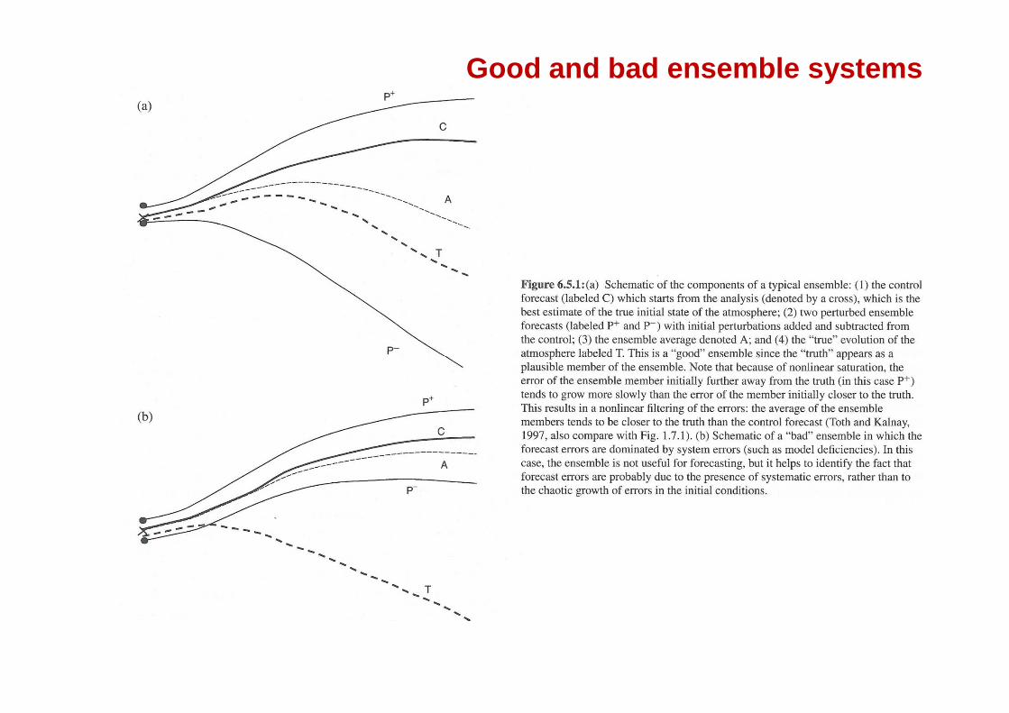
Good and bad ensemble systems

Initial-state perturbations; «monte carlo» and time-l agging.

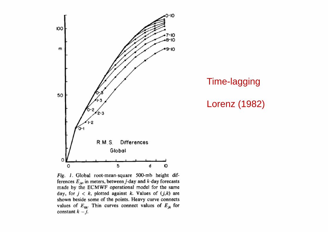
Time-lagging

Lorenz (1982)

Heterogeneous distribution of initial-state uncertainty .

Breeding

Self-breeding

Selective sampling: breeding vectors (NCEP)

At NCEP a different strategy based on perturbations growing fastest in the analysis cycles (bred vectors, BVs) was followed (now NCEP uses a different method called Ensemble Transformed with Rescaling, ETR, method). The breeding cycle was designed to mimic the analysis cycle.

Each BV was computed by (a) adding a random perturbation to the starting analysis, (b) evolving it for 24-hours (soon to 6), (c) rescaling it, and then repeat steps (b-c). BVs are grown non-linearly at full model resolution.

EC/TC/PR/RB-L2 2010 – Roberto Buizza: Approaches to ensemble prediction: the TIGGE ensembles80

Relation betweenBred-vector amplitudesand forecast error.

Bred vector alignment and growing instability

Selecting modes of instability by choosing the size of init ial state perturbations

SVs from more general inner products

Singular vectors can be defined as the result of

Singular Vectors

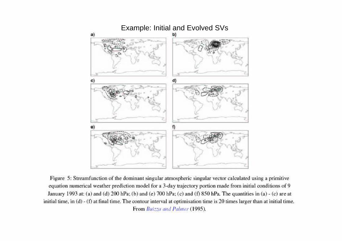
Example: Initial and Evolved SVs

Initial vs evolved SV total energy

Upscale developmentOf singular vectors

Amplification forsingular vectors& bred vectors

EDA=Ensemble Data Assimilation: parallel DA-cycles with perturbed observations

From PerssonFrom PerssonChapter 3

Reduced quality of perturbed initial state compared to main analysis

Can an alternative ensemble member beat the control forecast?

Ensemble mean vs. Individual categorical forecasts

Extreme forecast index (EFI)

The EFI is an integral measure of the difference between the ensemble forecast (ENS) distribution and the model climate (M-climate) distribution.

This allows the abnormality of the forecast weather situation to be assessed without defining specific (space- and time-dependant) thresholds. The EFI takes without defining specific (space- and time-dependant) thresholds. The EFI takes values from -1 to +1. If all the ensemble members forecast values above the M-climate maximum, EFI = +1; if they all forecast values below the M-climate minimum, EFI = -1.

Experience suggests that EFI magnitudes of 0.5 - 0.8 (irrespective of sign) can be generally regarded as signifying that "unusual" weather is likely whilst magnitudes above 0.8 usually signify that "very unusual" weather is likely.

Although larger EFI values indicate that an extreme event is more likely, the values do not represent probabilities as such.

Model Climate (M-Climate )For the calculation of EFI , M-climate is based on 9 consecutive semi-weekly re-forecast data sets (Mondays and Thursdays) consisting of 10+1 ensemble members, where the middle Monday or Thursday is the preceding Monday or Thursday closest to the actual ENS run date, t. The resolution decreases with forecast range exactly as in the ENS. This procedure allows seasonal variations and model changes to be taken into account, as well as model drift. Altogether 1980 re-forecast values are available for the M-cli mate computation (20 years x 11 ENS members x 9 semi-weeks). The M-climate is updated semi-weekly on Mon- and Thursdays. Mon- and Thursdays.

M-Climate= 9 semi-weekly, 11-member ENS, re-forcasts for previous 20 yearsThe figure shows an example when a Thursday is the closest, previous Mon- or Thursday

t t+30d

Thurs 0Thurs -1Thurs -2 Thurs +1 Thurs +2

11ens, 20yrs

Mon -2 Mon -1 Mon 0 Mon+1

From PerssonFrom PerssonChapter 5

The EFI: forecasted degree of extreme relative to climate data

EFI and median T2 daily meanValid Saturday 20 - Sunday 21 Feb 00utc, 2016

EFI and 99-percentile PrecipitationValid Saturday 20 - Sunday 21 Feb. 00utc, 2016

Error Growth

Kalnay, 6.6Kalnay, 6.6

Time-lagging

Lorenz (1982)

Representation of average model error

RMS-error:

With increasing forecast length t:


� So that for increasing t:

And for a bias-free model:

Error growth-model (Lorenz, 1982):

0.1

0.01

Models forForecastError growth

Lagged forecasts, 1981 and 2001

ECMWF

Ens-Means

Martin Leutbecher, ECMWF, private communication

Forecast day

High-res.deterministic

AC

C

Data Assimilation

Kalnay, Ch 5Kalnay, Ch 5+ a few notes

Basic principles

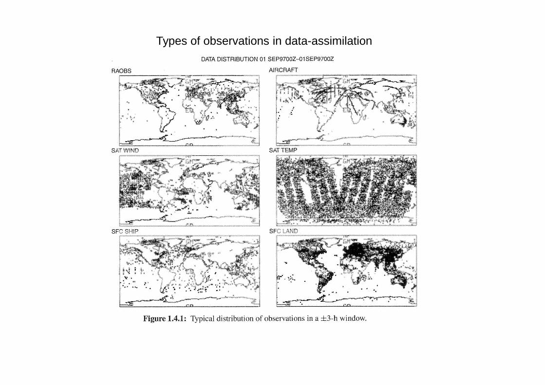
Types of observations in data-assimilation

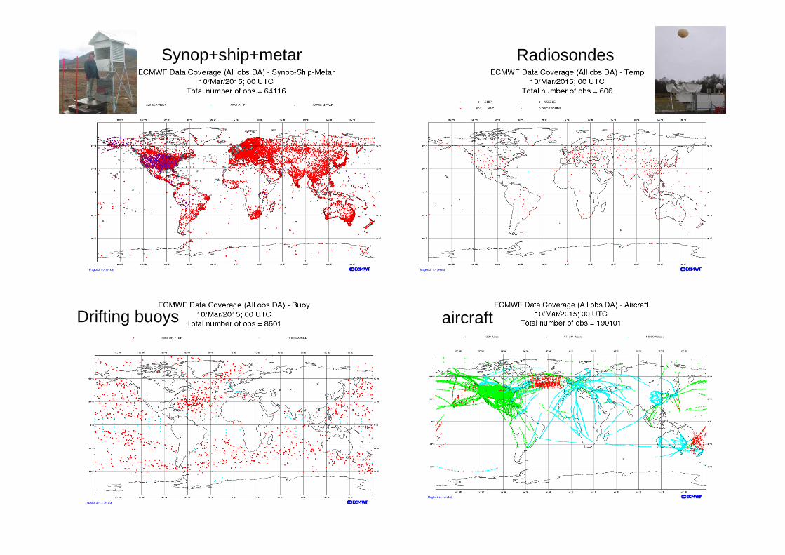
Synop+ship+metar Radiosondes

Drifting buoys aircraft

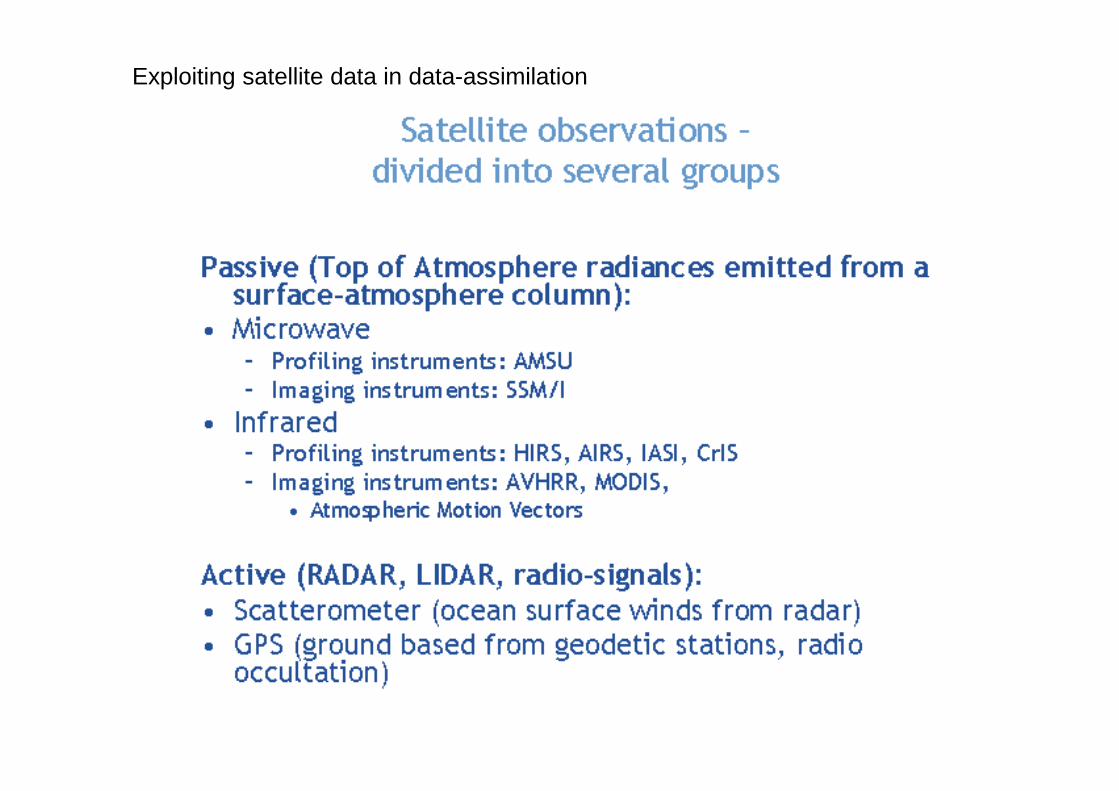
Exploiting satellite data in data-assimilation

AMSU-B AMSU-A

Microwaves

IASI

GPS -data

Scatterometer

VIS

IR

NH, PolarIR

AMV=AtmosphericMotionVectors

+ radiances

WVap

SH, PolarIR

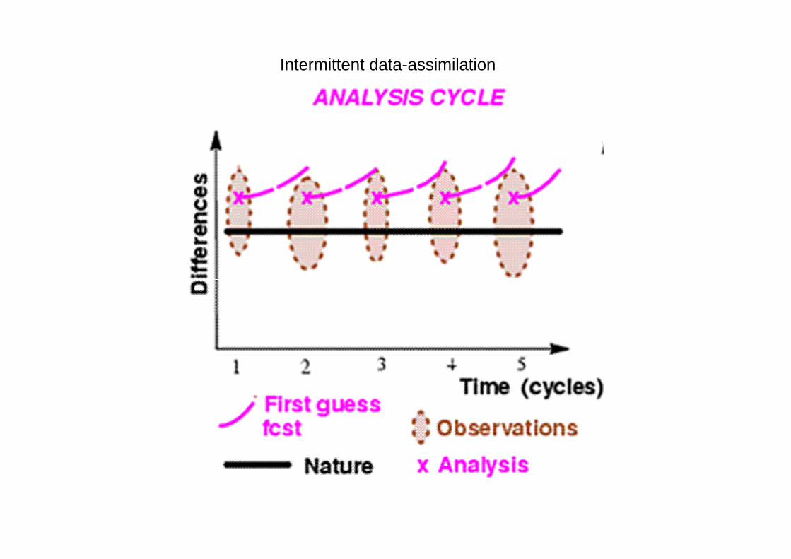
Intermittent data-assimilation

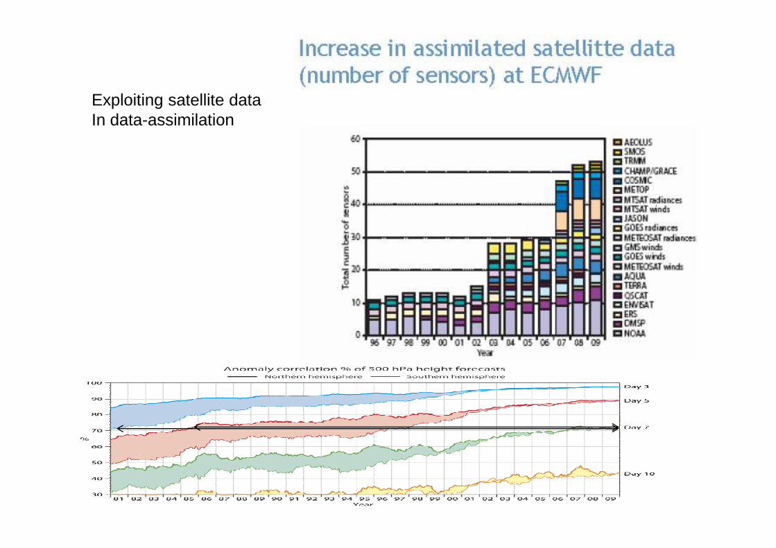
Exploiting satellite dataIn data-assimilation

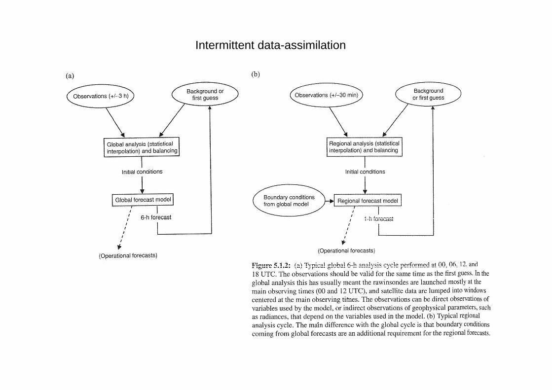
Intermittent data-assimilation

Reducing uncertainty by combining model data with observations

1 parameter

Multi-paramete r

N= model phase-space dim

P= obs phase-space dim

3DVar and 4DVarsimple presentation

Based on notes by A. Persson and F. Grizzini, ECMWF 2007

The analysis, A, defined by least-squares assumptionKalnay eqs.: (5.3.5), (5.3.9)

Find the value of S which minimizes J(S):δJ/δS = 0 for S = A

For any atmospheric state S, define:

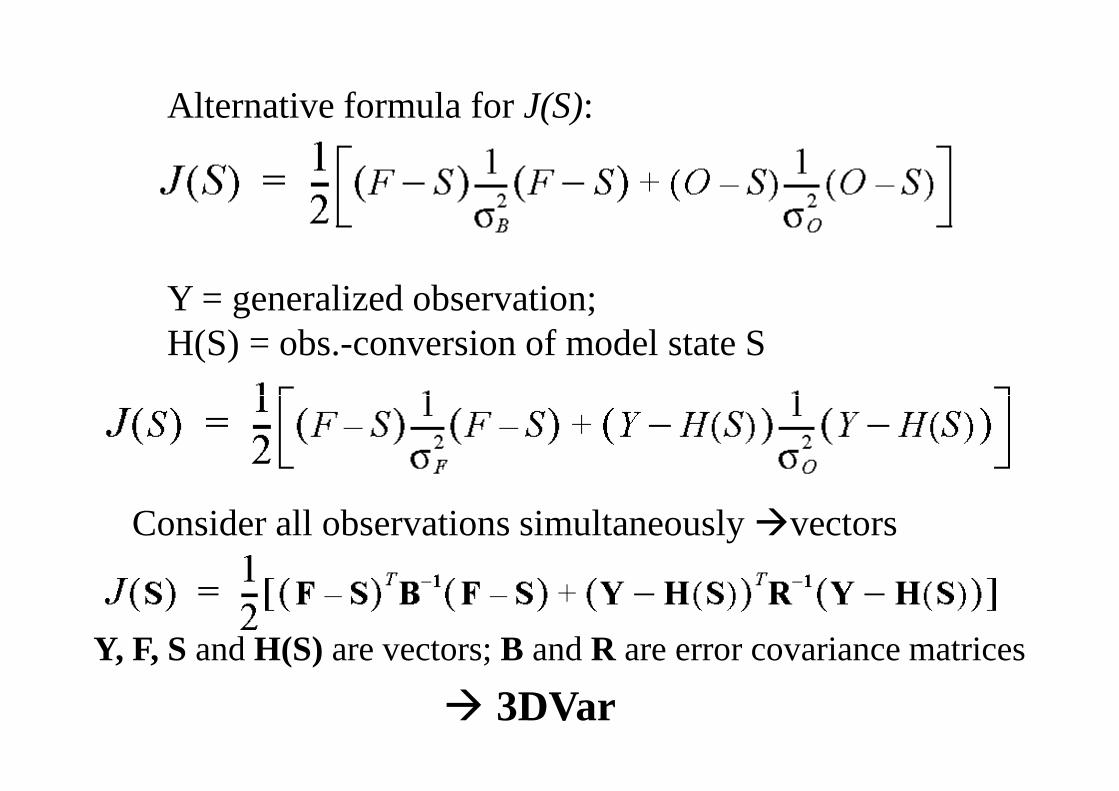
Alternative formula for J(S):

Y = generalized observation; H(S) = obs.-conversion of model state S

Consider all observations simultaneously �vectors

Y, F, S andH(S) are vectors; B and R are error covariance matrices

� 3DVar

Thanks to Adrian Simmons ECMWF

4DVar

Find a state S ( = A) which minimizes:

Mn = the modelled value at any time within the assimilation window.

Thanks to Adrian Simmons ECMWF

Extended and Long Range

ENSO: El Niño, Southern Oscilation

ENSO pattern and indices

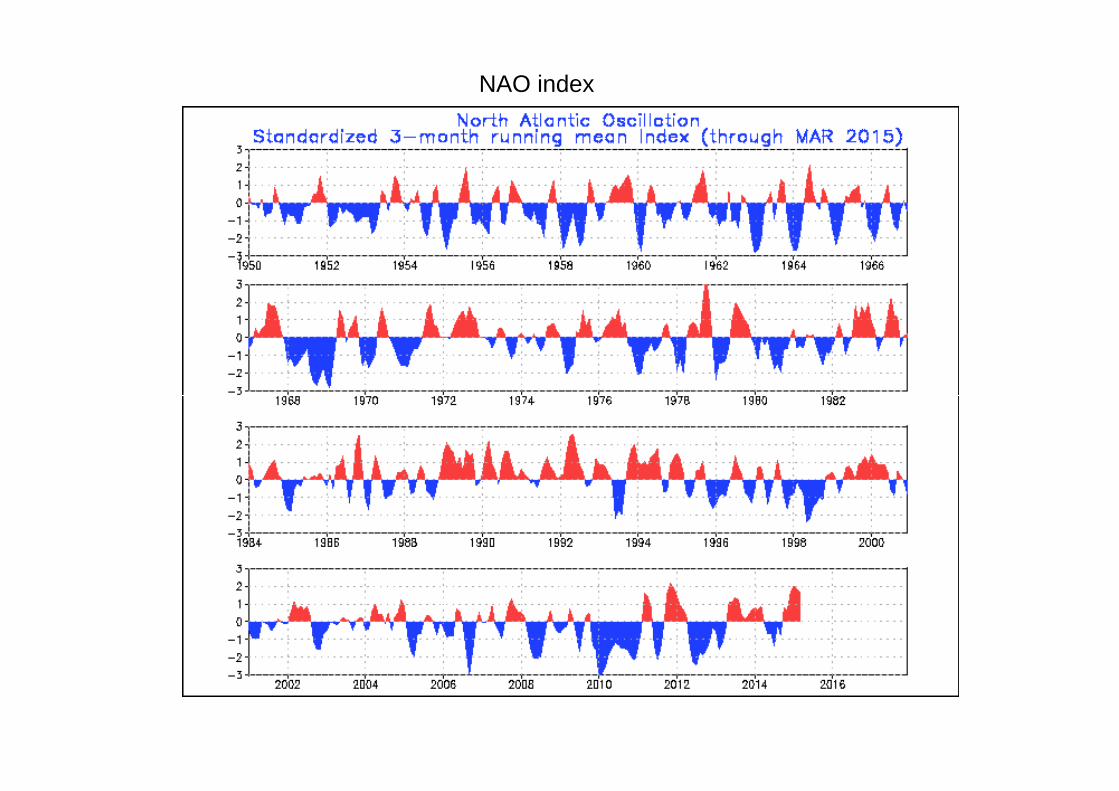
NAO index

MJO: Madden-Julian OscilationThe largest element of intraseasonal (30–90 day) variability in the tropical atmosphere

is characterized by an eastward progression of large regions of both enhanced and suppressed tropical rainfall, observed mainly over the Indian and Pacific Ocean.

Speculation being researched:

A Hovmöller diagram of the 5-day running mean of outgoing longwave radiation showing the MJO. Time increases from top to bottom in the figure, so contours that are oriented from upper-left to lower-right represent movement from west to east.

timeeastwards

Speculation being researched:

Potential connections betweenMJO and NAO.And potential source of intraseasonalpredictability in N-Atlantic and Europe

PNA Teleconnection patternENSO correlations

NAO Teleconnection pattern

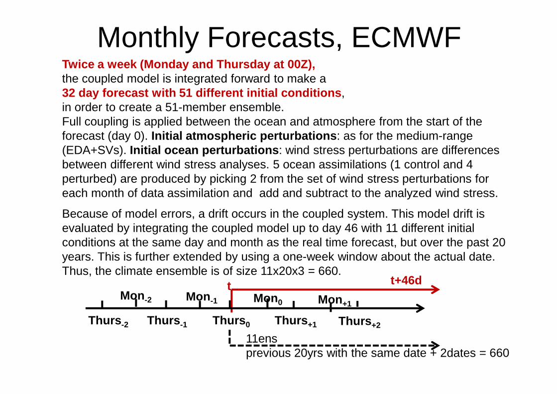
Monthly Forecasts, ECMWFTwice a week (Monday and Thursday at 00Z), the coupled model is integrated forward to make a 32 day forecast with 51 different initial condition s, in order to create a 51-member ensemble. Full coupling is applied between the ocean and atmosphere from the start of the forecast (day 0). Initial atmospheric perturbations : as for the medium-range (EDA+SVs). Initial ocean perturbations : wind stress perturbations are differences between different wind stress analyses. 5 ocean assimilations (1 control and 4 perturbed) are produced by picking 2 from the set of wind stress perturbations for each month of data assimilation and add and subtract to the analyzed wind stress.each month of data assimilation and add and subtract to the analyzed wind stress.

Because of model errors, a drift occurs in the coupled system. This model drift is evaluated by integrating the coupled model up to day 46 with 11 different initial conditions at the same day and month as the real time forecast, but over the past 20 years. This is further extended by using a one-week window about the actual date. Thus, the climate ensemble is of size 11x20x3 = 660.

t t+46d

Thurs 0Thurs -1Thurs -2 Thurs +1 Thurs +2

11ensprevious 20yrs with the same date + 2dates = 660

Mon -2 Mon -1 Mon 0 Mon+1

Temp & Prec anom, week 1 & 2starting from Monday 28. March 2016

Temp & Prec anom, week 3 & 4starting from Monday 28. March 2016

Z_500 anom, week 1, 2, 3 & 4 Weekly-mean 500hPa geopotential anomaly for the ensemble mean.

Contour intervals of 2dam (zero line not shown).starting from 28. March 2016

The plumes show the daily evolution of the ensemble forecast distribution, binned in 12.5% intervals (shading) together with the median (solid line).

starting from 28. March 2016

Seasonal Forecasts, ECMWFThe seasonal forecasts consist of a 51 member ensemble using a coarser-resolution version of the atmospheric model. The ensemble is constructed by combining the 5-member ensemble ocean analysis with SST perturbations and the activation of stochastic physics. The forecasts have an initial date of the 1st of each month, and run for 7 months . Forecast data and products are released at 12Z UTC on a specific day of the month. For System 4, this is the 7th.

Model-climate for bias-correction & anomaly-evaluat ionA set of re-forecasts are made starting on the 1st of every month for the years A set of re-forecasts are made starting on the 1st of every month for the years 1981-2010. They are identical to the real-time forecasts in every way, except that the individual date ensemble size is only 15 rather than 51. The total re-forecast ensemble size is thus: 15x30 = 450 .

An annual-range (13 months) forecast is made four times per year , with start dates the 1st February, 1st May, 1st August and 1st November, run as an extension of the seasonal forecasts, and are made using the same model but with a smaller ensemble size. Both re-forecasts and real-time forecasts and have an ensemble size of 15.The annual range forecasts are designed primarily to give an outlook for El Nino. They have an experimental rather than operational status.

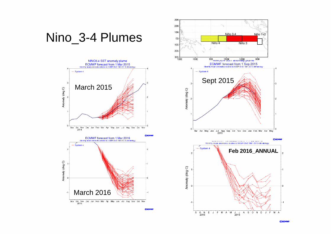
Nino_3-4 Plumes

March 2015Sept 2015

March 2016

Feb 2016_ANNUAL

NAOThe limits of the purple/grey whiskers and yellow band correspond to the 5th and 95th percentiles, those of the purple/grey box and orange band to the lower and upper tercile, while the median is represented by the line within the purple/grey box and orange band.

Northern Europe precip anomaly Northern Europe Temp anomaly

Prob relative to upper and lower terciles, JJA 2016T2m and Precip

T2<lower

Prec>upper

Prec<lower

T2>upper

From Predictions to Projections

(Decadal Climate Predictions)(Decadal Climate Predictions)

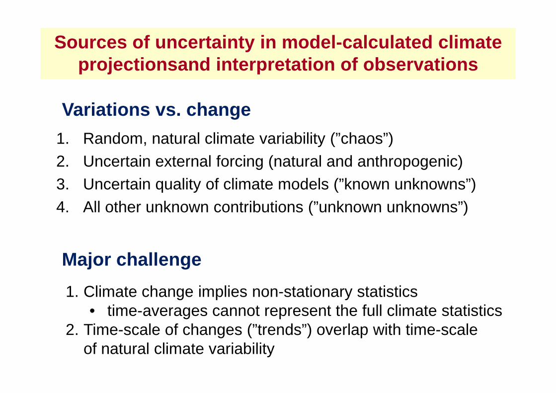
Sources of uncertainty in model-calculated climateprojectionsand interpretation of observations

1. Random, natural climate variability (”chaos”)2. Uncertain external forcing (natural and anthropogenic)3. Uncertain quality of climate models (”known unknowns”)

Variations vs. change

4. All other unknown contributions (”unknown unknowns”)

Major challenge

1. Climate change implies non-stationary statistics• time-averages cannot represent the full climate statistics

2. Time-scale of changes (”trends”) overlap with time-scaleof natural climate variability

Initial value vs forced boundary condition problem

Inertial commitment

RegionalInertialcommitments

Pacific decadal potential predictabilityLinked to solar forcing periodicity

Pacific decadal potential predictabilityLinked to internal variability (PDO / IPO)

AMO: Atlantic Multidecadal Oscilation Potential decadal predictability?

Atlantic MultidecadalOscillation index computed as the linearly detrendedNorth Atlantic sea surface

Schlesinger, M. E. (1994). "An oscillation in the global climate system of period 65-70 years". Nature 367 (6465): 723–726.

doi:10.1038/367723a0

surface temperature anomalies 1856-2013.

AMO and Atlantic Hurricanes

The number of tropical storms that can mature into severe hurricanes is much greater during warm phases of the AMO than during cool phases, at least twice as many. (Re.: NOAA)The hurricane activity index is highly correlated with the Atlantic multi-decadal oscillation. The AMO alternately obscures and exaggerates the global increase in temperatures due to human-induced global warming.[Chylek, P. & Lesins, G. (2008). "Multidecadal variability of Atlantic hurricane activity: 1851–2007". Journal of Geophysical Research 113: D22106. doi:10.1029/2008JD010036

The recent AMO increased the average number of Atlantic hurricanes and named storms from 6 to 12, when it began in 1995. This phase may have ended in 2012.

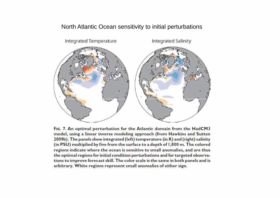
North Atlantic Ocean sensitivity to initial perturbations

Examples of decadal predictions . Recent efforts at decadal prediction, with the similar strategy: Initialize a global climate model from observations and reanalyses and run it forward 10 yr, while accounting for changes in external forcing (natural and anthropogenic).

Smith et al. (2007) showed that global-mean temperature could be predicted out to a decade in advance (Fig. 8a), with more skill than obtained when only external radiative forcing changes are accounted for.

Keenlyside et al. (2008) demonstrated that SST variations associated with the Atlantic MOC could be predicted a decade in advance, but because of an overly predicted a decade in advance, but because of an overly strong MOC signal, their strength was overestimated (Fig. 8b). Ten-year averaged global surface temperaturevariations were also predictable (Fig. 8a), but with marginally less skill than that obtained from radiativeforcing only.

In both studies forecasts were made for the next 10 yr (Fig. 8b), and in both cases natural internal variability was found to temporarily offsetanthropogenic global warming .The offset was largest in Keenlyside et al. (2008), whose results suggest a temporary lull in global warming for the next decade; however, the simplicity of the scheme employed needs to be kept in mind. The results of both studies highlight the impact ofinternal variability.

Contributions to uncertainty

Global vs regional

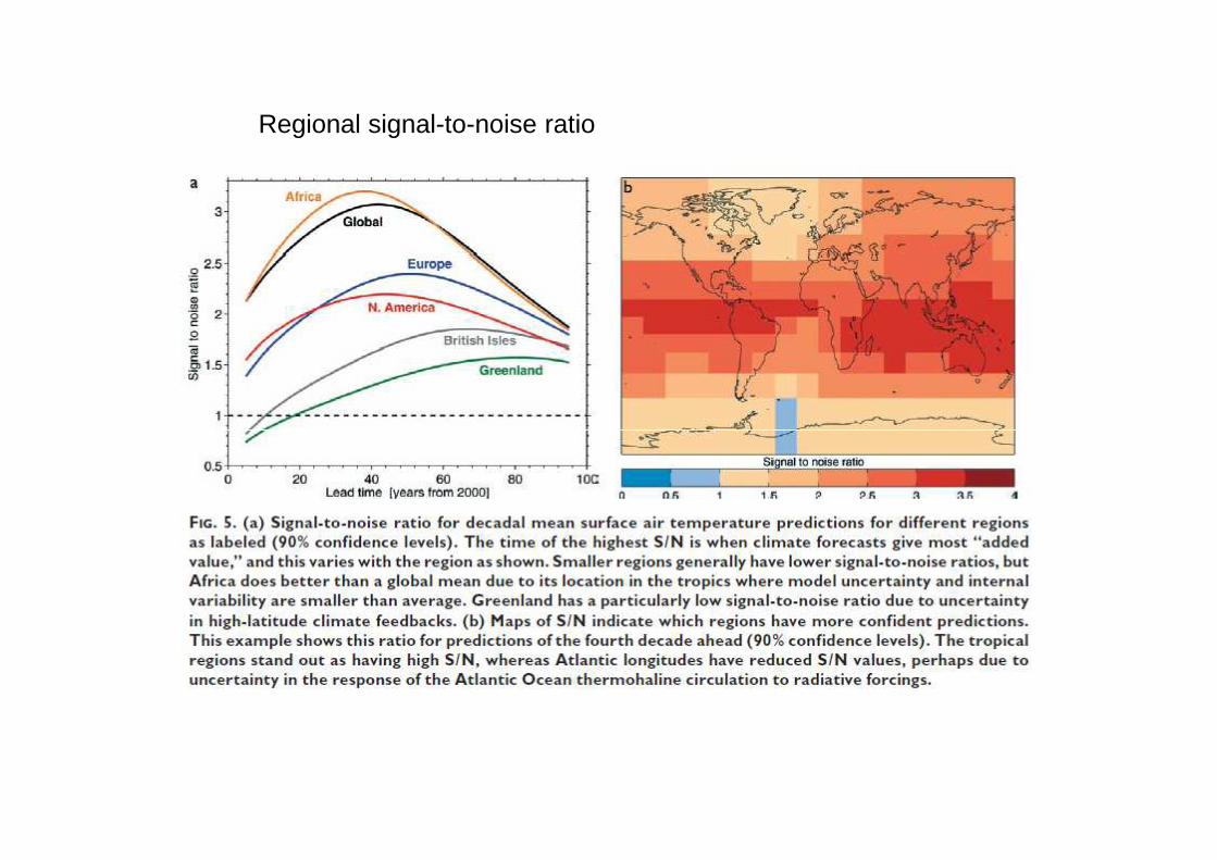
Regional signal-to-noise ratio

Relative contributions to variability and change at future time

The forecast being described here is from the experimental decadal prediction systemusing the latest Met Office climate model, HadGEM3, developed as part of the HadleyCentre Climate Programme. This system is at the cutting edge of research in understanding,simulating and predicting decadal variability.

It is only feasible to run the forecast out for the next 5 years .

NB: Produced in January 2014

It is only feasible to run the forecast out for the next 5 years .Furthermore, the number of ensemble members (10) is substantially less than that used inthe Met Office seasonal forecasting system (42). For these reasons the following resultsshould not be over-interpreted.

The decadal forecast produced in January 2014, for the 5-year pe riod 2014-2018 , isshown in Figure 1 as the set of dark blue lines, each representing an individual forecast fromthe 10-member ensemble. For comparison last year’s forecast (from January 2012) is shownin light blue lines.

The baseline 30-year mean climatology against which the forecast anomalies have beenexpressed, is1981-2010 , in line with WMO recommendations and other forecast products.

Figure 1: Global annual temperature record since 1960 and the latest ensemble of forecasts from the Met Office decadal prediction system produced in January 2014. The dark blue lines show the evolution of the 10 individual forecasts from this year’s forecast starting from November 2013 and the pale blue lines the equivalent for last year’s forecast. All data are rolling annual mean values.The gap between the black curves and blue curves arises because the last observed value represents the period November 2012 to October 2013 whereas the first forecast period is November 2013 to October 2014. The thin black curves show the observed annual-mean time-series from 3 independent datasets. Previous predictions starting from November 1960, 1965,..., 2005 are shown in red , and 22 Coupled Model Intercomparison Project phase 5 (CMIP5) model simulations that have not been initialized with observations are shown in green . In both cases, the shading represents the probable range, such that the observations are expected to lie within the shading 90% of the time. All temperatures are represented as anomalies from the 1981-2010 mean.

Decadal forecast; Forecast issued in January 2016.

•Averaged over the five-year period 2016-2020 , •enhanced warming over land, and at high northern latitudes;•some indication of continued cool conditions in the Southern Ocean, •relatively cool conditions in the North Atlantic sub-polar gyre. •global average temperature is expected to remain high; •Likely between 0.28°C and 0.77°C above the (1981-2010) average.

•(an anomaly of +0.44 ± 0.1 °C observed in 2015) •consistent with high levels of greenhouse gases and big changes currently underway in the climate system

Observed (black, from Met Office Hadley Centre, GISS and NCDC) and predicted (blue) from November 2015 global average annual surface temperature difference relative to 1981-2010. Previous predictions starting from November 2010. Previous predictions starting from November 1960, 1965, ..., 2005 in red, and 22 simulations from CMIP5 in green.Observations are expected to lie within the shading 90% of the time . Moving 12-month mean values.

Pacific Decadal Oscillation. Three-month averages of the monthly PDO index of Zhang et al. (1997) from 1900 to 2015. The same series after smoothing to retain decadal and longer variations is overlaid. The pair of curves at each end illustrate large uncertainty due to lack of data before and after the series.

The current developments in the worldwide pattern of sea surface temperatures are consistent with an emerging positive shift in the PDO , but it is too early to be confident that this will outlast the current El Niño.

Big Changes Underway in the Climate System?

Atlantic Multidecadal Oscillation . Values are annual average, area average North Atlantic sea surface temperature with the long-term linear warming trend removed (˚C), derived from the HadSST3 dataset (Kennedy et al., 2011a,b). The spread of values is a measure of the uncertainty arising from sampling and measurement errors. The solid lines show the low frequency AMO component.

The current trends suggest that the chances of a sh ift in the next few years have increased . However, it is not certain that there will be a shift towards cooler Atlantic conditions over the next few years. Temporary cooling has occurred in the past without leading to a sustained AMO shift.

Climate projections

Observational basis for a changing climate

The ”hockey-stick”

Continental air warmes faster than marine air

Updated to include 2015 (NASA/NOAA)"Since 1880, Earth’s average surface temperature has warmed by about 0.8 Celsius.The majority of that warming has occurred in the past three decades.“

“Earth's 2015 surface temperatures were the warmest since modern record keeping began in 1880” according to independent analyses by NASA's Goddard Institute for Space Studies and NOAA's National Centers for Environmental Information.

Climate Research Unit (CRU), Univ of East-Anglia, UKThe time series shows the combined global land and marine surface temperaturerecord from 1850 to 2015. This year was the equal warmest on record. This recorduses the latest analysis, referred to as HadCRUT.

Morice, C.P., Kennedy, J.J., Rayner, N.A. and Jones, P.D., (2012). Journal of Geophysical Research,117, D08101,doi:10.1029/2011JD017187

(The next warmest: 2014 +0.56 C)

2015 was the warmest year since modern record-keeping began in 1880, according to a new analysis by NASA’s Goddard Institute for Space Studies . The record-breaking

year continues a long-term warming trend — 15 of the 16 warmest years on record have now occurred since 2001. (Credit: NSA/GSFC/Scientific Visualization Studio)

Globally-averaged temperatures in 2015 shattered the previous mark set in 2014 by 0.23 degrees Fahrenheit (0.13 Celsius). Only once before, in 1998, has the new record been greater than the old record by this much.

Order of annual global mean Ts anomalies

Monthly (NOAA) global Ts-anomalies (rel.1951-80) during El Niño , La Niña , ENSO neutral (Nino3.4 index)

Variations above groundIPCC

Can models explain observed changes since1900? IPCC

Can models explain observed changes since 1900? IPCC

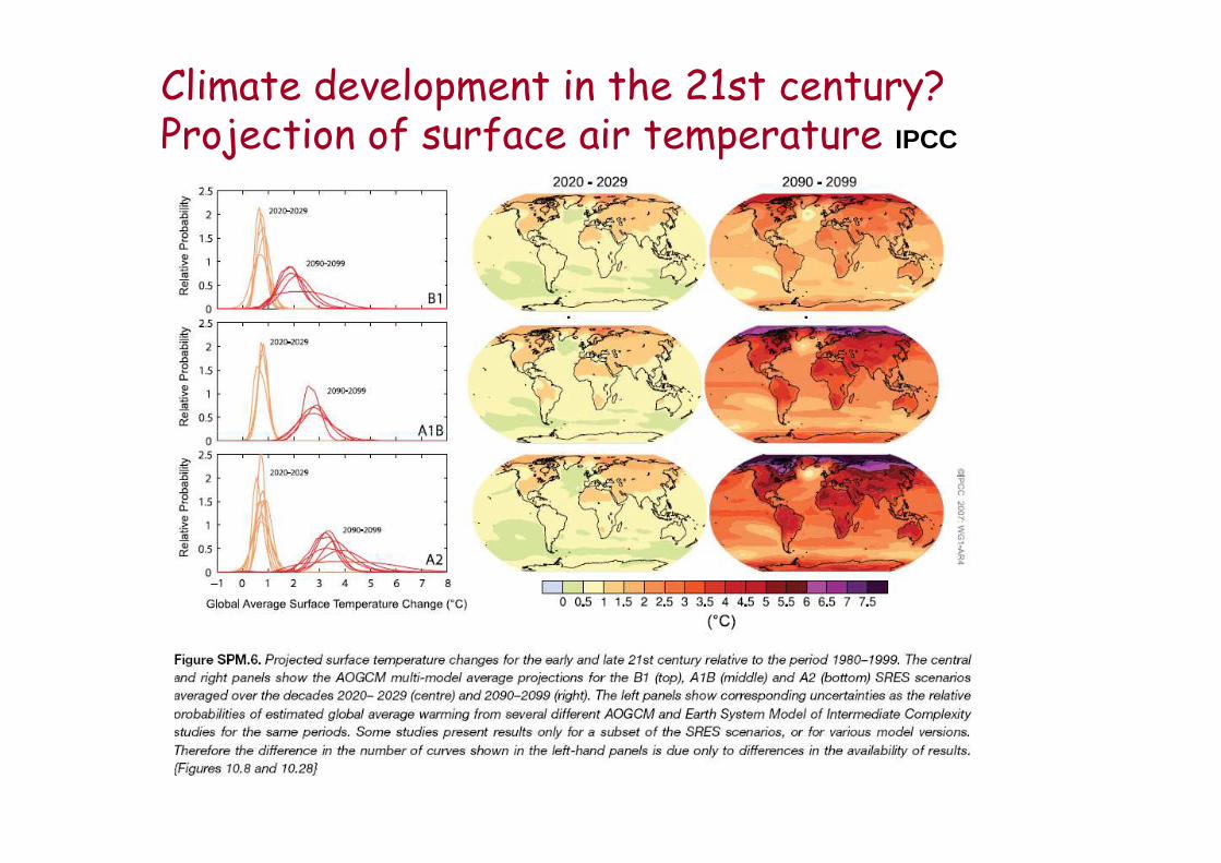
Climate development in the 21st century?Projection of surface air temperature IPCC

Climate development in the 21st century?Projection of precipitation change IPCC

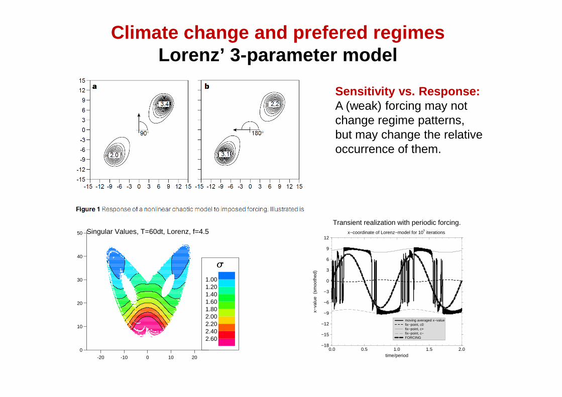
Climate change and prefered regimesLorenz’ 3-parameter model

Sensitivity vs. Response:A (weak) forcing may notchange regime patterns,but may change the relativeoccurrence of them.

-20 -10 0 10 20

0

10

20

30

40

50

2.602.402.202.001.801.601.401.201.00

Singular Values, T=60dt, Lorenz, f=4.5

0.0 0.5 1.0 1.5 2.0time/period

−18

−15

−12

−9

−6

−3

0

3

6

9

12

x−va

lue

(sm

ooth

ed)

Transient realization with periodic forcing.x−coordinate of Lorenz−model for 10

5 iterations

moving averaged x−valuefix−point, c0fix−point, c+fix−point, c−FORCING

forcing - response

Example:Amplification of Arctic warming by past air pollution reductions by past air pollution reductions in EuropeJC. Acosta Navarro, V. Varma, I. Riipinen, Ø. Seland, A. Kirkevåg, H. Struthers,T. Iversen, H-C. Hansson, A. Ekman

Nature Geosciences, March 15th, 2016.

Regional change in temperature when ∆Tglob = +2 °C

(°C, RCP8.5)

Notice the much larger temperature increase in the Arctic

Helge Drange, UiB:

Estimated probability for global Ts-decrease over 1 0 years, from 17 global climate models

PI-control, 1850 Historical, 1850-2010

Helge Drange, UiB:

RCP 2.6 RCP 4.5

RCP 6.0 RCP 8.5

Verifying probabilistic forecasts

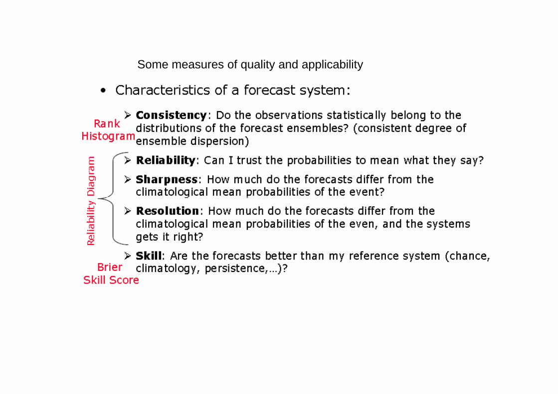
Some measures of quality and applicability

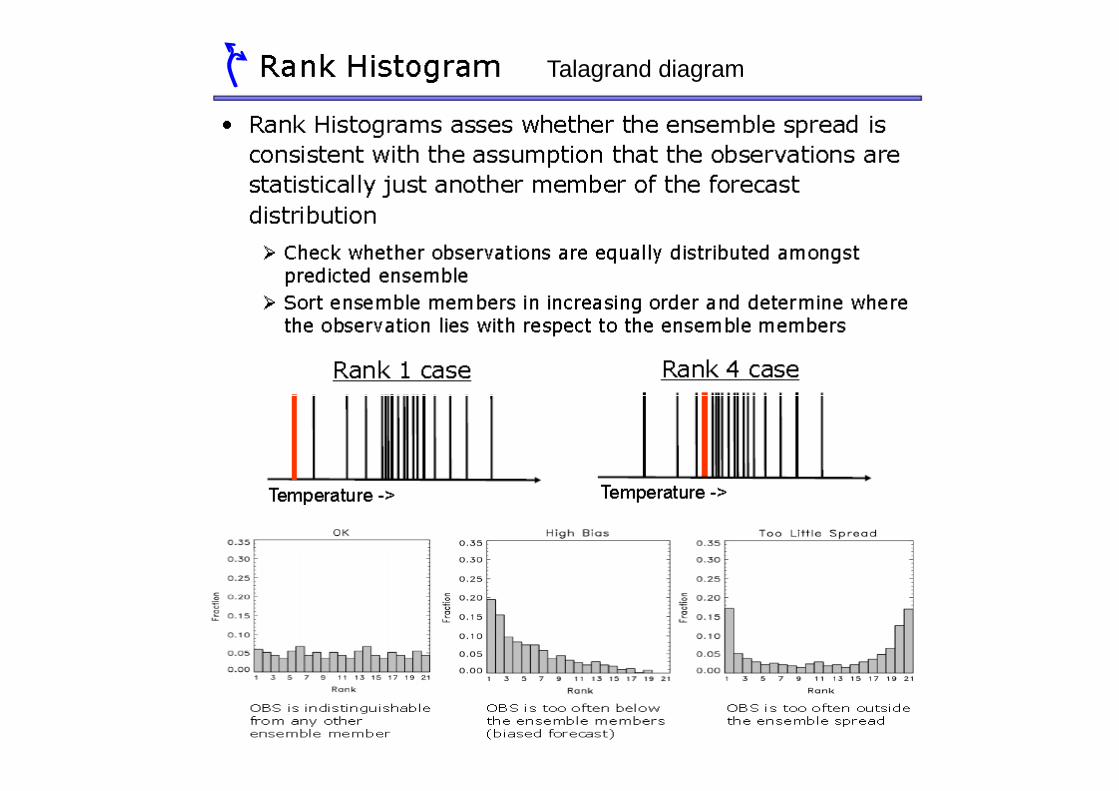
Talagrand diagram

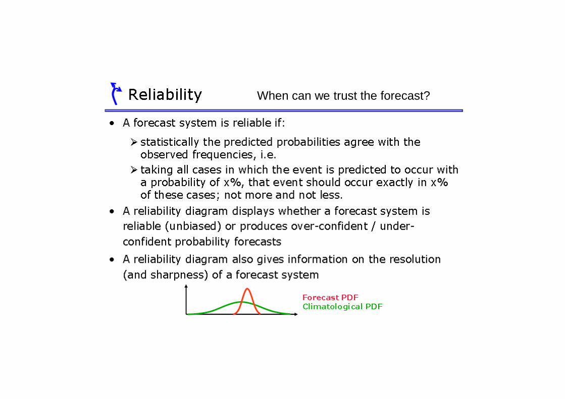
When can we trust the forecast?

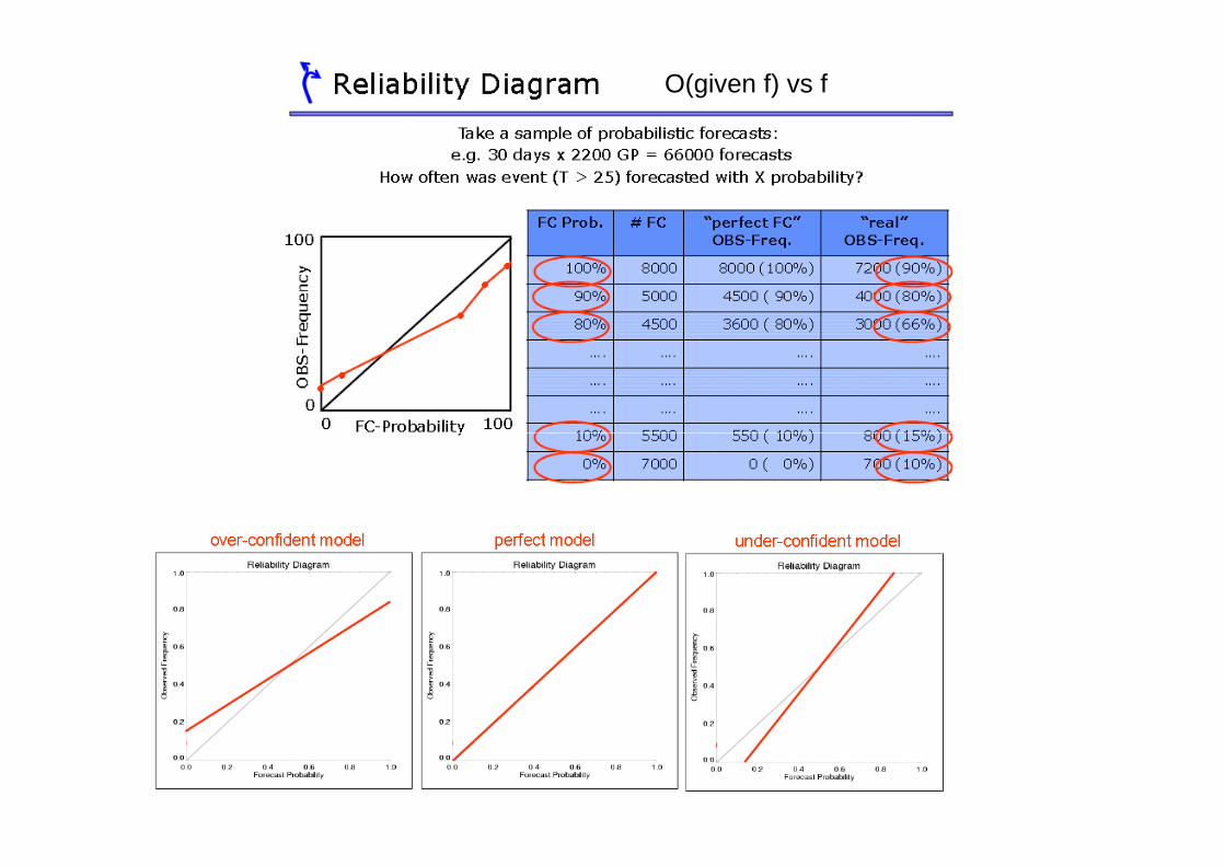
O(given f) vs f

BS

BSS

Reliability and Resolution

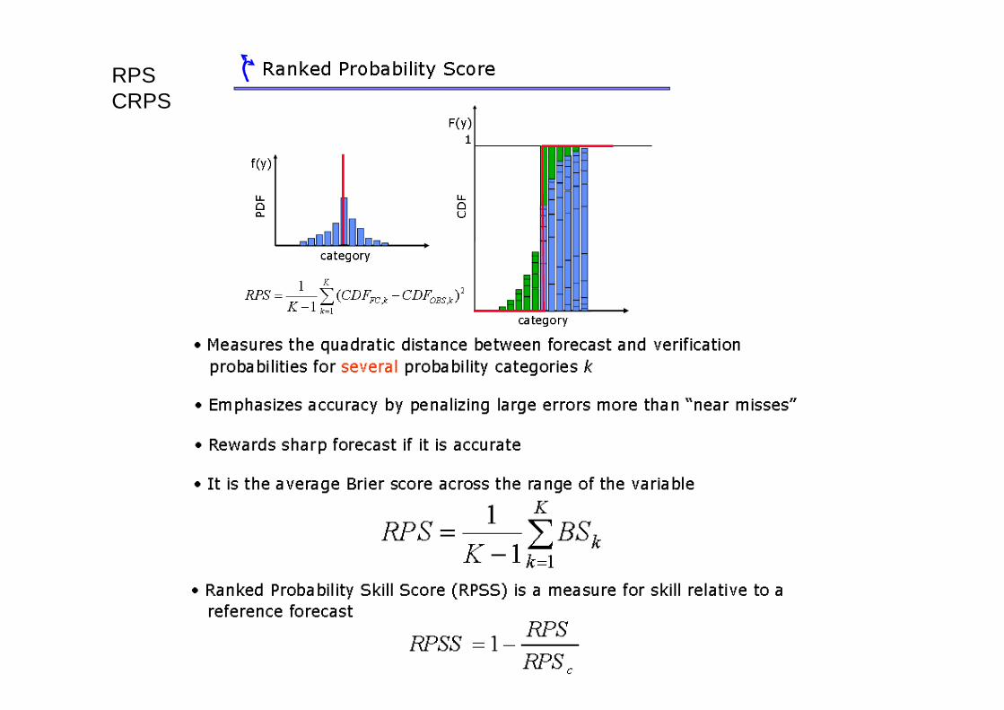
RPSCRPS

Benefits for different users - decision making

• A user (or “decision maker”) is sensitive to a specific weather event

• The user has a choice of two actions:

� do nothing and risk a potential loss L if weather event occurs

� take preventative action at a cost C to protect against loss L

• Decision-making depends on available information:

� no FC information: either always take action or never take action

deterministic FC: act when adverse weather predicted

Training Course 2007 – NWP-PR: Ensemble Verification193/24

� deterministic FC: act when adverse weather predicted

� probability FC: act when probability of specific event exceeds a certain threshold (this threshold depends on the user)

• Value V of a forecast:

� savings made by using the forecast, normalized so that

� V = 1 for perfect forecast

� V = 0 for forecast not better than climatology

Ref: D. Richardson, 2000, QJRMS

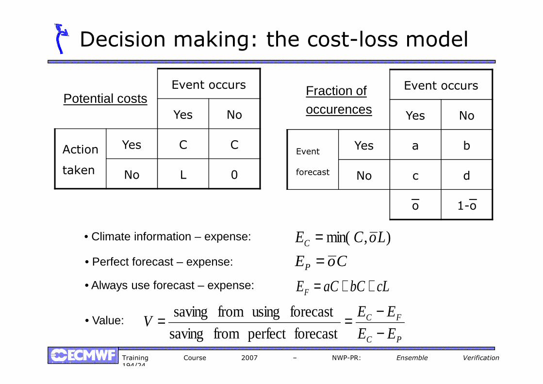
Decision making: the cost-loss model

Event occurs

Yes No

Action

taken

Yes C C

No L 0

Event occurs

Yes No

Event

forecast

Yes a b

No c d

Potential costsFraction ofoccurences


),min( LoCEC =• Climate information – expense:

cLbCaCEF ++=• Always use forecast – expense:

CoEP =• Perfect forecast – expense:

PC

FC

EE

EEV

−−==

forecastperfect from saving

forecast using from saving• Value:

o 1-o

PC

FC

EE

EEV

−−==

forecastperfect from saving

forecast using from saving

CC

C

o-L)o,min(

cL) bC (aC - L)o,min( ++=

ααααα o)-(1o)o-F(1 - )o,min( −+= H

with: α = C/L

H = a/(a+c) F = b/(b+d)ō = a+c

Decision making: the cost-loss model


αα o-)o,min(=

ō = a+c

0

0.1

0.2

0.3

0.4

0.5

0.6

0 0.2 0.4 0.6 0.8 1

C/L

valu

e

• For given weather event and

FC system: ō, H and F are fixed

• value depends on C/L

• max if: C/L = ō

• Vmax = H-F

Northern Extra-Tropics (winter 01/02)D+5 deterministic FC > 1mm precip

Potential economic value

0.1

0.2

0.3

0.4

0.5

0.6

valu

e

0.1

0.2

0.3

0.4

0.5

0.6

valu

e

Northern Extra-Tropics (winter 01/02) D+5 FC > 1mm precipitation

deterministic ENS

p = 0.2 p = 0.5 p = 0.8


0

0.1

0 0.2 0.4 0.6 0.8 1

C/L

0

0.1

0 0.2 0.4 0.6 0.8 1

C/L

0

0.1

0.2

0.3

0.4

0.5

0.6

0 0.2 0.4 0.6 0.8 1

C/L

valu

eENS: when each user chooses the most appropriate probability threshold

Brier Skill Score, EuropeT2m Prec24

+96h

Anomaly: >8K >4K <-4K <-8K Anomaly: >20mm >10mm >5mm >1mm

+144h

Brier Skill Score, +96h, starting from 1995. Against Analyses and observations in Europe

24h Nobs

Anomaly: >20mm >10mm >5mm >1mm

T850analyses

+144h+96h

Anomaly: >8K >4K <-4K <-8K

Brier Skill Score, against analyses and observations in Europe. Wind speed, 10m.

analyses

obs

+96h +144h

>10m/s

>15m/s

The forecast length (days) when CRPSS reaches smaller values than a given threshold for

24h precip and T 850hPa for NH and Europe

Precip0.112m MA

NH Extratropics Europe

T 8500.253m MA12m MA

Reliability-diagram and forecast sharpness, winter 2015

ff10mPrecip

+96h +96h>15m/s

>10m/s

>20mm >10mm >5mm >1mm

+144h +240h +144h +240h


ff10mPrecip

+96h +96h>15m/s

>10m/s

>20mm >10mm >5mm >1mm

+144h +240h +144h +240h

T2m


>8K >4K <-4K <-8K

+96h

+144h

+240h

Expected Value of + 144h forecasts of 24h precipitation in Europe with user’s c/L.

Winter 2015

1mm 5mm

ENS

10mm 20mm

HighRes

Expected Value of + 144h forecasts of 24h precipitation in Europe with user’s c/L.

Winter 2016

1mm 5mm

ENS

10mm 20mm

HighRes

EPS-meteograms ENS-meteograms - UiO

Documents

Transcript of EPS-meteograms ENS-meteograms - UiO