Electrochemical Impedance Spectroscopy Options

for Proton Exchange Membrane Fuel Cell

Diagnostics

by

JORGE IGNACIO VALENZUELA

B.A.Sc.. Electrical and Computer Engineering, University of British Columbia, 1993

B.Sc.. Physiology, University of British Columbia, 1988

A THESIS SUBMITTED IN PARTIAL FULFILLMENT OF THE REQUIREMENTS FOR THE DEGREE OF

MASTER OF APPLIED SCIENCE

in

The Faculty of Graduate Studies

(Electrical and Computer Engineering)

THE UNIVERSITY OF BRITISH COLUMBIA

November 2007

Jorge Ignacio Valenzuela, 2007

ii

Abstract

Electrochemical impedance spectroscopy (EIS) has been exploited as a rich source of

Proton Exchange Membrane Fuel Cell (PEMFC) diagnostic information for many years.

Several investigators have characterized different failure modes for PEMFCs using EIS

and it now remains to determine how this information is to be obtained and used in a

diagnostic or control algorithm for an operating PEMFC.

This work utilizes the concept of impedance spectral fingerprints (ISF) to uniquely

identify between failure modes in an operating PEMFC. Three well documented PEMFC

failure modes, carbon monoxide (CO) poisoning, dehydration, and flooding were

surveyed, modelled, and simulated in the time domain and the results were used to create a

database of ISFs. The time domain simulation was realized with a fractional order

differential calculus state space approach.

A primary goal of this work was to develop simple and cost effective algorithms that

could be included in a PEMFC on-board controller. To this end, the ISF was discretized

as coarsely as possible while still retaining identifying spectral features using the Goertzel

algorithm in much the same way as in dual tone multi-frequency detection in telephony.

This approach generated a significant reduction in computational burden relative to the

classical Fast Fourier Transform approach.

The ISF database was used to diagnose simulated experimental PEMFC failures into one

of five levels of failure: none (normal operation), mild, moderate, advanced, and extreme

from one of the three catalogued failure modes. The described ISF recognition algorithm

was shown to correctly identify failure modes to a lower limit of SNR = -1dB.

iii

Table of Contents

Abstract.................................................................................................................................ii

Table of Contents.................................................................................................................iii

List of Tables ....................................................................................................................... iv

List of Figures....................................................................................................................... v

Acronyms, Abbreviations, and Symbols ...........................................................................viii

Acknowledgements.............................................................................................................. ix

1 Introduction...................................................................................................................1

2 Fuel cell review.............................................................................................................4

3 Fault conditions ..........................................................................................................14

3.1 Dehydration ........................................................................................................14

3.2 Flooding..............................................................................................................17

3.3 Carbon monoxide poisoning...............................................................................19

4 Fuel cell time domain simulation ...............................................................................25

4.1 Non-integer order system response ....................................................................25

5 Electrochemical Impedance Spectroscopy .................................................................31

5.1 Obtaining the impedance spectra........................................................................32

5.2 Multi-frequency EIS techniques and noise.........................................................34

5.3 Multi-frequency EIS techniques and non-stationarity........................................36

5.4 Non-linearity and the multi-frequency stimulus waveform................................38

6 Goertzel algorithm based spectral analysis.................................................................40

6.1 The basic Goertzel algorithm .............................................................................40

6.2 Computation burden (memory and operations)..................................................43

6.3 Goertzel filter bank .............................................................................................44

7 Spectral fingerprint-based diagnostics........................................................................50

7.1 Spectral fingerprint evolution.............................................................................53

7.2 Failure mode identification via spectral fingerprinting ......................................56

8 Conclusions ................................................................................................................66

9 Suggestions for future work........................................................................................68

References...........................................................................................................................69

Appendix 1. Simulation of non-integer order transfer function ......................................73

Appendix 2. Equivalent circuit values from the literature ..............................................79

Appendix 3. Matlab program listings..............................................................................82

iv

List of Tables

Table 1.1 State of and contributions to the art in this investigation ....................................3

Table 3.1 Effects of dehydration on anode charge transfer resistance and membrane resistance.....................................................................................................................16

Table 3.2 Effects of flooding on cathode diffusion and charge transfer parameters.........18

Table 3.3 Effects of Carbon Monoxide contamination on anode diffusion parameters....22

Table 6.1 Computational and memory requirements of FFT and Goertzel algorithms.....44

Table 7.1 Computational and memory requirements of spectral fingerprint diagnostic algorithm.....................................................................................................................53

Table 7.2 Experimental failure mode detection challenges...............................................65

Table A2.1 Equivalent circuit parameters from the literature ...........................................81

v

List of Figures

Figure 1.1 Scope of investigation ........................................................................................2

Figure 2.1 Basic PEMFC operation.....................................................................................5

Figure 2.2 Graphical representation of the Butler-Volmer equation...................................6

Figure 2.3 Charge double layers in the PEMFC [5] ............................................................8

Figure 2.4 Simple PEMFC equivalent circuit......................................................................9

Figure 2.5 Schematic polarization curve for PEMFC .......................................................10

Figure 2.6 Polarization curve [12]. Operating points a – g described in Appendix 2 ......11

Figure 2.7 Bode plots of fitted equivalent circuit in Appendix 2 for operating points a, b, & c ..............................................................................................................................11

Figure 2.8 Bode plots of fitted equivalent circuit in Appendix 2 for operating points c, d, e, f & g ........................................................................................................................12

Figure 2.9 Nyquist plots of fitted equivalent circuit in Appendix 2 for operating points a & b. .............................................................................................................................12

Figure 2.10 Nyquist plots of fitted equivalent circuit in Appendix 2 for operating points c, d & e. ..........................................................................................................................13

Figure 3.1 Water management in PEMFC ........................................................................15

Figure 3.2 Effect of dehydration on PEMFC: Bode plot (a→e = normal→dehydrated) ..16

Figure 3.3 Effect of dehydration on PEMFC: Nyquist plot (a→e = normal→dehydrated)....................................................................................................................................17

Figure 3.4 Effect of flooding on PEMFC: Nyquist plot (a→e = normal→flooded) .........19

Figure 3.5 Effect of flooding on PEMFC: Bode plot (a→e = normal→flooded) .............19

Figure 3.6 Effect of CO contamination on PEMFC: Bode plot (a→e = normal→contaminated) ..............................................................................................23

Figure 3.7 Effect of CO contamination on PEMFC: Nyquist plot (a→e = normal→contaminated) ..............................................................................................23

Figure 4.1 Analytic and numeric solutions for Dα sin(x) with 2 times oversampling factor....................................................................................................................................26

Figure 4.2 Analytic and numeric solutions for Dα sin(x) with 10 times oversampling factor ...........................................................................................................................27

Figure 4.3 Analytic and numeric solutions for Dα sin(x) with 100 times oversampling factor ...........................................................................................................................27

Figure 4.4 Equivalent circuit for integer order software comparison...............................28

Figure 4.5 Comparison between commercial integer order simulation software and fractional order simulation software...........................................................................28

Figure 4.6 Equivalent circuit for non-integer order software comparison .......................29

vi

Figure 4.7 Comparison between analytical non-integer order frequency response versus Fourier transform of fractional order simulation software time domain output: Nyquist plot. ...............................................................................................................29

Figure 4.8 Comparison between analytical non-integer order frequency response versus Fourier transform of fractional order simulation software time domain output: Bode plot. .............................................................................................................................30

Figure 5.1 The frequency domain effect of time domain signal truncation ......................37

Figure 6.1 Frequency response and z-plane pole zero location: basic Goertzel algorithm42

Figure 6.2 Realization of basic Goertzel algorithm...........................................................42

Figure 6.3 Frequency response and z-plane pole zero location: modified Goertzel algorithm.....................................................................................................................43

Figure 6.4 Realization of modified Goertzel algorithm.....................................................43

Figure 6.5 Computational requirements of FFT and modified Goertzel algorithms for N = 4×106 ..........................................................................................................................44

Figure 6.6 Implementation of spectral analysis with Goertzel filter bank ........................45

Figure 6.7 Time domain representation of current stimulus and voltage response signals46

Figure 6.8 Impedance calculated via FFT and Goertzel algorithms..................................46

Figure 6.9 Noise performance of FFT and Goertzel algorithms .......................................47

Figure 6.10 Implementation of spectral analysis with Decimated Goertzel filter bank ....48

Figure 6.11 Noise performance of Decimated Goertzel algorithm ...................................49

Figure 7.1 Non-FRA-based PEMFC diagnostics ..............................................................50

Figure 7.2 Discrete frequency points requirement ............................................................52

Figure 7.3 Non FRA based PEMFC diagnostics using Goertzel and EIS fingerprint recognition ..................................................................................................................52

Figure 7.4 Five spectral fingerprints at increasing stages of CO PEMFC poisoning (SNR=0dB).................................................................................................................54

Figure 7.5 Five spectral fingerprints at increasing stages of CO PEMFC poisoning (SNR=–1.5dB)............................................................................................................54

Figure 7.6 Five spectral fingerprints at increasing stages of PEMFC dehydration (SNR=0dB).................................................................................................................55

Figure 7.7 Five spectral fingerprints at increasing stages of PEMFC dehydration (SNR=–1.3dB) .........................................................................................................................55

Figure 7.8 Five spectral fingerprints at increasing stages of PEMFC flooding (SNR=0dB)....................................................................................................................................56

Figure 7.9 Five spectral fingerprints at increasing stages of PEMFC flooding (SNR=–1.5dB) .........................................................................................................................56

Figure 7.10 Spectral fingerprint matching during normal PEMFC operation (SNR=0dB)....................................................................................................................................57

Figure 7.11 Spectral fingerprint matching during PEMFC CO poisoning (SNR=0dB) ...58

vii

Figure 7.12 Spectral fingerprint matching during PEMFC CO poisoning (SNR=-1.5dB)59

Figure 7.13 Spectral fingerprint matching during PEMFC Dehydration (SNR=0dB)......60

Figure 7.14 Spectral fingerprint matching during PEMFC Dehydration (SNR=-1.3dB) .61

Figure 7.15 Spectral fingerprint matching during PEMFC Flooding (SNR=0dB) ...........62

Figure 7.16 Spectral fingerprint matching during PEMFC Flooding (SNR=-1.5dB) .......63

Figure 7.17 Spectral fingerprint matching during PEMFC Dehydration (SNR=0dB)......64

Figure A1.1 One electrode of PEMFC ..............................................................................73

viii

Acronyms, Abbreviations, and Symbols

EIS Electrochemical impedance spectroscopy

FRA Frequency response analyzer

STFT Short term Fourier transform

FFT Fast Fourier transform

DSP Digital signal processing

PEMFC Proton exchange membrane fuel cell

TPB Triple phase boundary

PFTE Polytetrafluoroethylene

T Temperature

F Faraday’s constant

R Universal gas constant

αa Anodic transfer coefficients

io Exchange current density

i Current density

Rct,a Charge transfer resistance, anode

BV Butler-Volmer

Aeff Effective area

dH Helmholtz layer thickness

εo Permittivity of free space

εr Relative permittivity

Cdl Double layer capacitance

Rel Electrolyte resistance

Rs Series resistance

s Laplace variable

A(i) Warburg resistance (also denoted as σ)

δ Diffusion film thickness

τ Time constant of diffusion

Deff Effective diffusion constant

λc Stoichiemtric coefficient, cathode

θx Adsorption fraction species x

GL Grünwald-Letnikov

SNR Signal to noise ratio

IIR Infinite impulse response

DFT Discrete Fourier transform

CNLS Complex non-linear least squares

ix

Acknowledgements

I would like to thank my supervisors, Dr. W.G. Dunford and Dr. W. Merida for their

patience and guidance throughout this project.

My colleagues, Tatiana Romero and Javier Gazzarri have been constant sources of fruitful

discussion and challenging questions. I offer my sincere thanks to them for their

participation and friendship.

For most of my adult life Chris Parks, Klaus Kallesøe and Gordon White have been the

brothers I wish my parents had begat. I thank you all for your great friendship and

diligent efforts to maintain it despite my lack of availability over the last few years.

My parents and sister deserve a great deal of thanks for everything they have done for me

during this and my previous degrees. Without question, if I stand tall, it is only because I

can stand on their shoulders.

Finally, and certainly not least, I would like to thank my wife, Maria Alicia Silva. She has

been a constant source of love, inspiration, support, and good humour throughout the last

9 years of my life. Without her, none of this would have been possible or even

worthwhile.

1

1 Introduction

Fuel cells convert chemical energy from hydrogen, methanol, diesel, gasoline, etc. into

electrical energy. While fuel cells are capable of very high conversion efficiencies in both

stationary and mobile applications, the automotive application is the most anticipated

application due to the elimination of harmful atmospheric emissions. Apart from the

obvious questions about hydrogen generation and the materials issues that plague fuel

cells, questions arise with regard to how the system is going to be tested and controlled in

the field.

Many different electrochemical techniques have been used to study fuel cells. These

include current interrupt, cyclic voltammetry, electrochemical impedance spectroscopy

(EIS), Raman spectroscopy, etc. Of these, the impedance spectrum provides one of the

richest sources of information about electrochemical systems. In addition, the non-

invasive nature of EIS makes it a valuable diagnostic tool.

Complex impedance values are usually obtained by exciting the electrochemical system

with a single frequency sinusoidal voltage or current signal and measuring the current or

voltage respectively. This same process is carried out sequentially by a frequency

response analyzer (FRA) for each frequency of interest until the desired operating

frequency range scan is complete. The EI spectrum is then fitted to an equivalent circuit

or distinct frequency bands are compared to determine the state of health of the fuel cell

(Figure 1.1). This approach is unsuitable for embedded diagnostics use for two reasons:

first, the equipment involved is cumbersome and expensive; second, the measurement is

lengthy and often, the state of the fuel cell evolves during the measurement. There are

techniques available to mitigate this latter problem while still using FRA-based EI

spectroscopy [1, 2], but they involve additional testing and digital signal processing that

further increases the experimental duration and computation burden.

Despite the fact that fuel cell non-stationarity imposes a measurement challenge, the

information useful to designers and to real-time control systems is precisely that which is

embedded within the time-varying impedance data. For example, as the fuel cell

membrane dehydrates, it loses efficiency and drops power output. At the same time, the

2

polymer electrolyte membrane impedance increases and can thus be used as a signal to

increase the humidification.

Many researchers have approached this problem from the perspective of the Short Time

Fourier Transform (STFT). This approach employs the Fast Fourier Transform (FFT) of

time domain system input-output data multiplied by an appropriate short time window to

obtain the impedance spectrum at discrete slices of time. As with FRA-based EIS, this

spectrum is then fitted to equivalent circuits or distinct frequency bands are compared.

Unfortunately, this approach while more suitable than traditional FRA-based EIS

diagnostics, still imposes a sizeable computational burden on the diagnostic equipment.

FC freq-domain impedance model FRA-EIS

STFT-EIS

Goertzel-EISFC time domain model

Impedance spectral fingerprint analysis

FC equivalent circuit model

Equivalent circuit fitting

Bandpass filter output ratios

Figure 1.1 Scope of investigation

This investigation extends the work of Popkirov, Schindler, Darowicki and others on the

STFT by employing an alternate digital signal processing (DSP) method to obtain the

electrochemical impedance spectrum: the Goertzel algorithm (highlighted in bold in

Figure 1.1). Further, the EI spectrum thus obtained is analyzed in much the same way as

fingerprints are used to identify criminals within the justice system. Like the use of

fingerprinting in criminal processes, this requires (i) uniqueness of the fingerprint, and (ii)

the prior characterization of the EI spectrum for each failure mode; the fingerprint

database. To evaluate this approach, equivalent circuit models for the fuel cell under

normal and fault conditions are obtained from the literature. These equivalent circuit

models are used in two ways (Figure 1.1): First, they give rise to a reference frequency

domain impedance spectrum. Since this spectrum is calculated via a closed form analytic

expression, it does not suffer from any bias or variance imposed by a spectral estimation

algorithm. Second, they provide the parameters for a time domain state space model that

3

allows us to simulate the time domain response of the fuel cell to an EIS stimulus signal.

The spectral estimates of the simulated time domain response obtained via Goertzel

algorithm can be evaluated against the theoretical reference spectrum.

It is hypothesized that these improved approaches should be more suitable for use in a

real-time, on-board, impedance-based fuel cell diagnostic module than the traditional

STFT approach because of the decreased computational burden, elimination of complex

least squares equivalent circuit fitting procedures, and increased specificity of spectral

content analysis.

In the following chapter, we review the required fuel cell specific information such that

we can put subsequent impedance models into physical context. In chapter 3 we describe

the fuel cell failure modes to be considered and their respective equivalent circuit impacts.

In chapter 4 we create a time-domain fuel cell simulator that allows us to create datasets

for testing of our EIS diagnostic routines under controlled and specified fault conditions.

In chapter 5, we explore EIS in both its development and diagnostic role. In chapter 6, we

apply the Goertzel algorithm to the EIS problem and compare the results with the classical

STFT method. In chapter 7, we develop a multi-dimensional spectral fingerprint control

space based on the EIS data from chapter 6.

Table 1.1 State of and contributions to the art in this investigation

State of the art Contribution Chapter

Use of the Short Time Fourier Transform (STFT) to calculate experimental EI spectral results

Use of the Goertzel algorithm (borrowed from telephony) to reduce computational burden

6

Integer and fractional1 order time domain simulation of PEMFC behaviour

Fractional order time domain simulation of PEMFC behaviour

4

Up to 4 EIS frequency band diagnostic algorithms.

EIS spectral fingerprint based diagnostics 7

1 There are errors in the derivation of the published fractional order simulation algorithm. We have had personal communications with the article author highlighting the error and we have included the complete, correct derivation in Appendix 1.

4

2 Fuel cell review

The polymer electrolyte membrane fuel cell (PEMFC) will be used as a model for the

present investigation, but the signal processing approach discussed in this paper can be

applied to any fuel cell system including solid oxide, molten carbonate, direct methanol,

formic acid, phosphoric acid, etc. A brief summary of the operation of the PEMFC is

provided to lay the foundation for the equivalent circuit approximations employed later.

For greater detail concerning losses, thermodynamics, heat management, kinetics,

catalysis, water balance, etc., the reader is referred to other references [3-5].

Figure 2.1 shows the basic elements of the PEMFC. We can consider it to be a system in

which the controlled oxidation of hydrogen via an electrochemical process results in

useful electrical work according to the chemical reactions (2.1) through (2.3).

( ) ( )2 2 aqgH H + 2e−+ 0.000 SHEV (2.1)

( ) ( )1

22 2 aqgO H ++ + 2e−+ ( )2 @1.229 SHEg STP

H O V (2.2)

( ) ( ) ( )21

2 2 22 1.229e

g g gH O H O V−

+ (2.3)

The fuel cell itself consists of three basic elements: the anode, the electrolyte, and the

cathode. The anode contains a gas diffusion layer through which the humidified gas

travels and encounters the triple phase boundary (TPB) where the fuel gas, solid catalyst

(usually platinum), and aqueous electrolyte phases meet. It is at this point that the

hydrogen molecule gives up two electrons that travel through the external circuit (the

electrolyte is ionically conductive but not electronically conductive). The resulting

protons diffuse along their concentration gradient and migrate along the electric field

Figure 2.3 through the electrolyte to the cathode TPB where they combine with oxygen

and electrons to form water. The resulting cell potential is 1.229V at standard temperature

and pressure.

The PEMFC employs a sulfonated polytetrafluoroethylene (PTFE) membrane (e.g.,

Nafion by Dupont) as the electrolyte. This membrane must be sufficiently hydrated that

ionic conduction of the protons is possible. At the same time, the anode and cathode

TPBs must be sufficiently dry that the gas phase is not occluded from the solid catalyst.

5

Humidification is controlled by oxidant gas flow (higher air flow results in greater

evaporation at the cathode thus drying out the membrane) and by direct humidification of

the fuel and/or oxidant gas streams.

Figure 2.1 Basic PEMFC operation

The Butler-Volmer (BV) equation (2.4) governs the kinetics of the hydrogen oxidation

(2.1) and oxygen reduction (2.2) reactions

0

a cs s

F F

RT RTi i e eα αη η−

= −

(2.4)

where T is the temperature in K, F is Faraday’s constant, R is the universal gas constant,

αa and αc are the anodic and cathodic transfer coefficients, respectively, i0 is the exchange

current density, i is the current density through the fuel cell, and ηs is the surface (or

activation) overpotential [6]. The BV current-voltage relationship is plotted in Figure 2.2.

A detailed examination of the kinetic (Eq.(2.4) and Figure 2.2) and physical (Figure 2.3)

properties of the electrode interface reveals several elements that we will re-cast into an

electronic model (Figure 2.4) for ease of interpretation and prediction.

The inverse of the slope of the voltammogram (Figure 2.2) gives the first element in our

electronic model or equivalent circuit: the polarization resistance or charge transfer

resistance, Rct (Figure 2.4). Specifically, the value of Rct (2.6) can be calculated from the

6

small signal ( )0.05s voltsη < approximation of the BV equation (2.5). This expression is

obtained by ignoring the second order and greater terms in the Taylor series expansion of

the BV equation

0

0Linear region

Fue

l cel

l cur

rent

den

sity

(A

/cm

2 )

Overpotential (V)

Figure 2.2 Graphical representation of the Butler-Volmer equation

( )0a c s

i Fi

RTα α η= + (2.5)

giving

( )0

sct

a c

RTR

i i F

ηα α

= =+

(2.6)

This element represents an electrochemical reaction that traverses the electrode electrolyte

interface and therefore represents a pathway for DC. Since i0 varies proportionally with

reaction rate, a small Rct implies a kinetically favourable reaction.

The charge transfer resistance is calculated at the null potential (open circuit) where it is

maximal and decreases with current density. When the fuel cell is polarized (i.e., a load

current is being drawn), the small signal approximation fails and we turn to the Tafel

approximation

0ln ln as

Fi i

RT

α η= + (2.7)

for anodic ( )20 , 0s volts i A cmη −> > ⋅ polarization [6]. From this expression, we obtain

1s

cta

d RTR

di F i

ηα

= = (2.8)

7

indicating that the charge transfer resistance decreases with increasing load current. This

demonstrates that impedance spectra are functions of current density and any spectral

fingerprint-matching algorithm must take this into account.

While the electrodes and the electrolyte are both close to electroneutral, the region near

the electrode-electrolyte interface is not (Figure 2.3). The mobile charges are

electrostatically attracted to the oppositely charged species in the adjacent phase. These

charges accumulate at the interface and, owing to the charge separated by their solvated

ionic radii2, an electric field is established. This charge separation can be modelled as a

capacitor. Since the charge distribution is not along a perfect parallel plate, but rather a

rough surface, the deep invaginations of which limit the penetration of mobile ions due to

size and diffusion lag, the capacitor model departs from the ideal giving rise to the so-

called constant phase element3. For the purposes of this investigation, however, we shall

treat this element as an ideal capacitor

o r effdl

H

AC

d

ε ε= (2.9)

where Aeff is the surface area, which is different from the nominal geometric electrode area

owing to the catalyst loading, availability, and roughness of the electrode surface, εo and εr

are the permittivity of free space and the relative permittivity respectively, and dH is the

Helmholtz layer thickness4. This element is in parallel with the charge transfer resistance

because current can traverse the electrode-electrolyte interface by either mechanism

Figure 2.4.

2 These species are usually weakly bound to water molecules further increasing their effective ionic radii. In fact, the electric field in the double layer is so strong that it aligns the water molecules according to their dipole moment in a very uniform layer. 3 The parallel plate capacitor analogy is further complicated by the fact that the cations (H+) are mobile, while the anions (hydrated sulfonyl group on Nafion polymer) is immobile. The PEMFC cathode double layer is therefore somewhat of a mystery. 4 Gouy and Chapman argued this layer would be diffuse owing to a statistical distribution of ionic species near the metal-liquid interface. Later, Stern showed that there would be a charge-free region defined by the often solvated ionic radius of the ionic species involved.

8

Figure 2.3 Charge double layers in the PEMFC [5]

The voltage at each point along the cell width is depicted schematically below Figure 2.3.

The double layers are depicted as having similar widths, but different accumulated charge

densities. However, it must be stressed that the true shape of these potential curves is

unknown and is an area of active research5. Additionally, the slopes in the electrodes and

the electrolyte are non-zero owing to the non-zero resistance of these regions.

The hydrogen ions diffuse and migrate across the electrolyte through an aqueous

sulfonated PTFE matrix. The small channels formed by the hydrophilic regions of the

PTFE polymer chain permit proton transport, but the tortuousness of the proton

conduction path gives rise to a resistance, Rel. This resistance is a function of ionic

concentration (or water content since the solute is fixed), temperature, and stack clamp

pressure. This is a purely linear resistance and the lost energy is dissipated as heat. Since

this resistance is in series with all the other elements of the fuel cell, we lump it together

5 Additionally, the distribution of anions is more complex than it seems in the diagram because the sulfonyl groups in Nafion are not mobile, but fixed. The ionic species that populate the double layer boundary is therefore not certain. See Appendix 2.

9

with the other pure resistances (bipolar plates and gas diffusion electrodes) and rename it

Rs in our equivalent circuit (Figure 2.4).

Finally, we must consider mass transfer effects. Consider the reactant species involved in

the reactions at the anode or the cathode. At the cathode, the oxygen must diffuse in the

gas phase and the hydrogen ions must diffuse in the aqueous phase to the triple phase

boundary (TPB) where the electrons can join them and, in the presence of the platinum

catalyst, form water. Hydrogen gas diffusion at the anode is very fast and does not limit

the reaction rate to any significant extent. Water, however, is required to transport the

products of the hydrogen reduction reaction at the anode and its availability is often

limited by electro-osmotic drag mediated dehydration at the anode. It is the diffusion of

water that most affects the value of the Warburg impedance under normal conditions [7].

These mass transfer effects can be modelled using the analogy between a resistive

capacitive transmission line and Fick’s law. The result is the finite Warburg impedance

( ) ( ) ( )tanhW

sZ s A i

s

τ

τ= (2.10)

where s is the Laplace variable, and A(i) is a non-linear function of current density, i [8, 9]

and

2 effDτ δ= (2.11)

is the time constant of diffusion with δ representing the thin film thickness6 and Deff, the

effective diffusion coefficient.

Rct

Cdl

ZW

Rs

Rct

Cdl

ZW

Anode Electrolyte Cathode

Figure 2.4 Simple PEMFC equivalent circuit

6 Not to be confused with the Helmholtz layer thickness, dH

10

While the impedance of the anode electrode-electrolyte interface is neglected in many

investigations, we have retained these elements in our equivalent circuit model because

the anode is significantly affected by some of the fault conditions that we will simulate. It

is important to note that most of these equivalent circuit parameters change with DC

operating point in addition to changing with fault conditions.

Three principal regions in the PEMFC polarization curve (Figure 2.5) can be identified:

the Activation, Ohmic, and Mass Transfer Limited regions. The evolution of impedance

with current density can be observed by noting the overvoltages (voltage losses)

associated with each of these regions. In the activation region, cathode activation

impedance dominates and the Ohmic and Warburg impedance are negligible. In the

ohmic region, activation impedance drops and is roughly constant, ohmic impedance is

constant and Warburg impedances are still negligible. Lastly, in the Mass Transfer

Limited region, the Warburg impedance begins to grow rapidly [3, 5, 10]. Most PEMFCs

are operated at or near peak power, near the end of the ohmic region.

Cell current density (A·cm2)

Cel

l vol

tage

(V

)

ηcathode

ηanode

ηohmic

ηmass transfer

Ohmic region

← Activation region

Mass transfer region →

← Power

Figure 2.5 Schematic polarization curve for PEMFC

In this study, the equivalent circuit of Figure 2.4 has been fitted to EIS data from the

literature [9, 11-13] to provide a model with which to examine the signal processing

routines described herein (see Appendix 2). The frequency response (Figure 2.7 and

Figure 2.8) of the fitted equivalent circuit is plotted (Figure 2.6) at several operating points

in the activation (a,b), ohmic (c,d,e), and the beginning of the mass transfer limited

regions (f,g).

11

0 100 200 300 400 500 6000

0.2

0.4

0.6

0.8

1

Cel

l vol

tage

(V

)

ab c

de

f

g

0 100 200 300 400 500 6000

80

160

240

320

400

Pow

er (

mW

·cm−

2 )

Current Density (mA·cm2)

Figure 2.6 Polarization curve [12]. Operating points a – g described in Appendix 2

10−2

10−1

100

101

102

Imp

ed

an

ce (Ω

)

a

b

c

10−3

10−2

10−1

100

101

102

103

104

−80

−60

−40

−20

0

Frequency (Hz)

Ph

ase

(d

eg

ree

s)

Figure 2.7 Bode plots of fitted equivalent circuit in Appendix 2 for operating points a, b, & c

12

0.01

0.02

0.03

0.04

0.05

0.06

Imp

ed

an

ce (Ω

)

c

d

e

f

g

10−3

10−2

10−1

100

101

102

103

104

−40

−30

−20

−10

0

Frequency (Hz)

Ph

ase

(d

eg

ree

s)

Figure 2.8 Bode plots of fitted equivalent circuit in Appendix 2 for operating points c, d, e, f & g

0 0.5 1 1.5 2 2.5 3 3.5 4 4.5 5 5.5 60

0.5

1

1.5

2

2.5

3

Real(Z) (Ω)

−Im

ag(Z

) (Ω

)

a

b

c

d

e

Figure 2.9 Nyquist plots of fitted equivalent circuit in Appendix 2 for operating points a & b.

13

0 0.005 0.01 0.015 0.02 0.025 0.03 0.0350

0.005

0.01

Real(Z) (Ω)

−Im

ag(Z

) (Ω

)

a

b

c

d

e

Figure 2.10 Nyquist plots of fitted equivalent circuit in Appendix 2 for operating points c, d & e.

In summary, a conceptual PEMFC equivalent circuit model was created from the literature

and the electrochemical origins of the classical Randles cell components were described.

This model goes beyond those typically reported in the literature in that it includes all

potential equivalent circuit elements rather than a reduced set as in many investigations.

In this manner, variation of any parameter, regardless of the relative magnitude of its

spectral effect, can be evaluated. Finally, values for the equivalent circuit parameters

were derived from data reported in the literature and it was shown that the theoretical EI

spectra coincide well with spectra reported in the literature (Appendix 2).

14

3 Fault conditions

We are concerned with faults that begin to manifest electrically within minutes of the

onset of the fault condition. Long-term degradation processes that occur on a time scale

of thousands of hours of operation are not considered. Long term deterioration, however,

cause gradual increases of both Rct,a and Rct,c owing to both reversible and irreversible

mechanisms. This complicates fault detection for on-board implementations of the

methods discussed in this investigation in that “normal” fuel cell operation must be

continually redefined or measured.

Schulze et al. have shown that there are both reversible and irreversible mechanisms

involved in the long-term degradation of the fuel cell. The irreversible degradation is

caused by agglomeration of the platinum catalyst [7]. Having suffered such degradation,

the presence of carbon monoxide at the fuel cell anode is more pronounced (see section

3.3) because the effective platinum loading is reduced. For the purposes of this

investigation, this effect will be treated as negligible since the increase in Rct,a owing to

long term irreversible degradation is fourfold over a 1000 hour period, whereas the CO

poisoning effect on Rct,a is two orders of magnitude over a few hours [14].

The reversible degradation process is mostly associated with membrane hydration state

and recovers after shut down and re-start and will not be considered further.

3.1 Dehydration

Water management is one of the most critical elements of PEM fuel cell design [3, 15-17].

Water can enter the PEMFC via the anode and cathode gas streams and is produced at the

cathode by the oxygen reduction reaction (Eqn. (2.2) & Figure 3.1). It exits the PEMFC

via evaporation, primarily at the cathode. Water management is further complicated by

electro-osmotic drag of water from the anode to the cathode. This means that despite a net

production of water in the PEMFC and the counteracting diffusion and convection

processes, the anode becomes progressively dehydrated. Further, electro-osmotic drag

increases linearly with current density such that the problem is more difficult to manage at

high loads. The contrary is true of the cathode. It will progressively flood, especially at

high load currents, unless water is removed. Dehydration has several deleterious effects

15

on durability and reliability that we seek to prevent by careful monitoring of hydration

[18, 19]. Two main effects of dehydration manifest themselves in PEMFCs.

Anode Electrolyte Cathode

H2O Diffusion

H2O Convection

H2O Electro-osmotic dragH2O in

H2O out

H2O in

H2O out

H2O from ORR

Figure 3.1 Water management in PEMFC

First, as the cell dehydrates, the proton conduction channels in the PTFE matrix constrict

increasing Rs. As mentioned earlier, the increased resistance produces losses that are

dissipated as heat. In extreme cases, parts of the membrane become so heated that

membrane drying accelerates which, in turn, further exacerbates the dehydration problem.

The heat permanently damages the proton conduction channels in the membrane and can

even result in catastrophic failure of the PEMFC due to perforation of the membrane

resulting in an inability to maintain reactant separation.

Second, as the electrolyte is dehydrated the anode TPB begins to dry out and either

destroys TPBs by eliminating the liquid phase or makes TPB “islands” (i.e., H+ is

produced, but it cannot reach the electrolyte) [16]. This drop in catalytic efficacy is

manifest as an increase in Rct,a in our equivalent circuit. Some representative results from

the literature are summarized in Table 3.1.

16

Table 3.1 Effects of dehydration on anode charge transfer resistance and membrane resistance

% ∆ in Rct,a Rs

Investigator Notes

16.7 9.3 [13] A=28cm2, j=500mA·cm2, Pa=Pc=1atm, T=75°C, (dry cathode and anode), H2/O2

24.1 16.1 [17] A=50cm2, j=200mA·cm2, T=80°C, ∆RH=74%, Nafion 117, H2/O2 flow=200cm3·min-1,

16.1 64 [20] Hydrogenics series 500 stack (1 cell), j=400mA·cm2, Pa,Pc=121.3kPa, T=65°C, dry H2 & O2 gas feed, λa=1.2, λc=2

31.3 71.9 [21] A=150cm2, j=467mA·cm2, Pa=Pc=1atm, T=60°C, RHa=10%,

RHc=15%, λa=1.2, λc=4, H2:Air

Andreaus recommends minimizing electrolyte thickness and membrane equivalent weight

in order to maximize the back diffusion of water thus preventing dehydration [13]. For a

given fuel cell design, however, the control strategy is limited to modifying humidification

of gas feeds or stoichiometric ratios thus requiring minimal lag humidity detection which

is the object of this study.

0.01

0.02

0.03

0.04

0.05

Imp

ed

an

ce (Ω

)

a

b

c

d

e

10−3

10−2

10−1

100

101

102

103

104

−30

−25

−20

−15

−10

−5

0

Frequency (Hz)

Ph

ase

(d

eg

ree

s)

Figure 3.2 Effect of dehydration on PEMFC: Bode plot (a→e = normal→dehydrated)

17

0 0.005 0.01 0.015 0.02 0.025 0.03 0.035 0.04 0.0450

0.005

0.01

Real(Z) (Ω)

−Im

ag(Z

) (Ω

) a

b

c

d

e

Figure 3.3 Effect of dehydration on PEMFC: Nyquist plot (a→e = normal→dehydrated)

Using a 0 to 50% linear increase in Rs and 0 to 20% linear increase in Rct,a we simulate

progressive dehydration with time under dehydrating conditions (e.g., dry gas feeds).

Bode plots of spectra from dehydrated PEMFCs are characterized by an increase of cell

impedance magnitude across all frequencies and an increase (less capacitive) in phase

angle in the mid to high frequencies. The dehydration effect is equally visible in the

Nyquist plot, which shows a right lateral shift by the amount of the membrane resistance

increase. The anode charge transfer resistance does not manifest on the graph because the

cathode charge transfer resistance is orders of magnitude larger and masks the anode

contribution to the overall PEMFC faradaic impedance. The spectra shown in Figure 3.2

and Figure 3.3 are consistent with published results in the references in Table 3.1.

3.2 Flooding

Under high load conditions, fuel cell current density increases and the production of water

at the cathode by oxygen reduction reaction (2.2) and by electro-osmotic drag increases

(Figure 3.1). Unchecked, this can lead to flooding of the GDL. The initial stage of

flooding is characterized by a slow decrease in output voltage as liquid water begins to

accumulate in the GDL and constrict the gas flow channels thus increasing the diffusion

related equivalent circuit parameters Ac(i) and τc. Additionally, some TPBs are lost as the

gas phase becomes occluded from the solid catalyst and liquid electrolyte thus raising Rct,c.

This process occurs over minutes [16, 22-24].

When the GDL channels become completely blocked, the subsequent stage of flooding

manifests as a drastic voltage drop over the course of seconds [20-22]. This fault

condition is especially damaging if allowed to develop fully because the fuel cell can go

into reversal (-ve output voltage). This can result in electrolysis instead of oxygen

18

reduction, localized heating and permanent damage to the cell. The reversal mechanism

can damage both the membrane and the catalyst layer [25] and lead to long term

degradation effects [7]. Detection of the flooding condition by simple voltage monitoring

(first stage) has been proposed, but it is not as fast or sensitive as an EIS-based diagnostic

when operating at high current levels [21, 22].

Recovery from this latter stage of flooding failure is effected by a high pressure pulse of

reactant gas to clear the channel [5]. However, preventing this extent of failure by

increasing oxidant gas (typically air) flow to exaggerate evaporation while the flooding is

still in the initial stages is the primary goal of humidification control. There are few

studies in the literature devoted to EIS of flooding PEMFCs. Fewer still fit the EI spectral

data to the Randles cell. Two such results are presented in Table 3.2 [15, 20]7.

Table 3.2 Effects of flooding on cathode diffusion and charge transfer parameters

% ∆ in Ac(j) τc Rct,c

Investigator Notes

817 8.07 104 [21] A=150cm2, j=467mA·cm2, Pa=Pc=1atm, T=60°C, RHa=70%, RHc=50%, λa=1.2, λc=4, H2:Air

1200 - 150 [20] Hydrogenics series 500 stack (1 cell), j=400mA·cm2, Pa,Pc=121.3kPa, T=65°C, λa=1.2, λc=2→1.18

We use a 0 to 900% linear increase in Ac(j) and 0 to 100% linear increase in Rct,c to

simulate progressive cathode gas diffusion channel flooding with time under flooding

conditions (e.g., reduced λc). Bode plots of spectra from dehydrated PEMFCs are

characterized by an increase of low frequency cell impedance magnitude and a decrease in

phase angle (more capacitive) in the mid to low frequencies. The flooding effect can be

related to equivalent circuit parameter changes in the Nyquist plot, which shows the

growth of the high frequency loop dominated by Rct,c and Cdl,c as well as a growth of the

diffusion resistance, Ac(j), characterized by an increase in the size of the low frequency

loop with its associated 45° slope on the left edge. The spectra shown in Figure 3.4 and

Figure 3.5 are consistent with published results in the references in Table 3.2.

7 Merida did not report an increase in Rct,c as observed in other studies, but the impairment of diffusion (↑Ac(j) & ↑τc) was observed (15. Merida, W.R., Diagnosis of PEMFC stack failures via electrochemical impedance spectroscopy, in Mechanical Engineering. 2002, University of Victoria: Victoria.)

19

0 0.01 0.02 0.03 0.04 0.05 0.06 0.07 0.08 0.09 0.1 0.11 0.12 0.13 0.14 0.15 0.160

0.01

0.02

0.03

Real(Z) (Ω)

−Im

ag(Z

) (Ω

) a

b

c

d

e

Figure 3.4 Effect of flooding on PEMFC: Nyquist plot (a→e = normal→flooded)

10−2

10−1

Impe

danc

e (Ω)

a

b

c

d

e

10−3

10−2

10−1

100

101

102

103

104

−40

−30

−20

−10

0

Frequency (Hz)

Pha

se (

degr

ees)

Figure 3.5 Effect of flooding on PEMFC: Bode plot (a→e = normal→flooded)

3.3 Carbon monoxide poisoning

The use of pure hydrogen to power fuel cell vehicles is problematic for three reasons.

First, on-board storage is not yet as simple, reliable, and inexpensive as comparable

hydrocarbon storage and it has a lower gravimetric and volumetric power density.

Second, widespread distribution of hydrogen is not yet available although it can be argued

that if the market manifests a need, the energy companies will follow. Third, pure

hydrogen is not readily available in nature and must be obtained either from hydrocarbon

sources by reforming reactions or from renewable sources which, at present, lack power

20

density. For at least the early stages of fuel cell commercialization, then, hydrogen supply

will be largely from existing hydrocarbons such as methane via the endothermic reforming

reaction

( )2 22n mmC H n H O nCO n H+ → + + (3.1)

This carbon monoxide (CO) contaminates the fuel cell platinum catalyst via the

exothermic water gas shift reaction

2 2 2CO H O CO H+ → + (3.2)

by occupying platinum metal (M in (3.3)) catalyst sites to the exclusion of hydrogen [26,

27].

2

2 2

2 2

2

| | |

| | | | | |

| | 2

adjacent sites

dissolved

linear adsorbedadsorbed H O

CO

activated complexadjacent sites

H O CO H O

CO M

M M M

CO H O CO H O e CO OH e H

M M M M M M

CO OH

CO e H M

M M

− − +

− +

+ + →

+ +→ →

→ + + +

⋯ ⋯ ⋯

⋯

(3.3)

The rate of hydrogen oxidation in the presence of CO is given by

( )2 2

21H

COH COi i θ= − (3.4)

where θx is the adsorption fraction of species x. Since the hydrogen oxidation reaction

(2.1) is so much faster than CO oxidation, it controls the surface potential when θCO is

small. When θCO increases, the overpotential grows until it reaches that which is required

to oxidize CO [27, 28].

21

Careful hydrogen reformer design reduces the concentration of CO in reformate gas feeds

from parts per hundred to parts per million [29, 30], but this amount is still sufficient to

limit the hydrogen reaction rate due to the preferential adsorption of CO over hydrogen

together with the lack of a spontaneous CO removal mechanism. Thus, while the

overpotential of the CO-free anode (hydrogen oxidation) reaction is typically orders of

magnitude lower than the cathode (oxygen reduction) reaction, CO poisoning increases

the anode overpotential by two orders of magnitude resulting in considerable reduction in

output power [27].

Several CO-poisoning mitigation strategies have been studied including: elevation of fuel

cell temperature thus increasing the rate of the water gas shift reaction, incorporating

catalyst alloys designed to favour the water gas shift reaction, and bleeding O2 to oxidize

the CO to CO2 thus liberating the catalytic site for hydrogen oxidation. The first of these

strategies cannot be used with the low temperature range Nafion membrane and require

special high temperature PE membranes [31]. The second of these CO-tolerant schemes

involves the incorporation of Ru or Mo into the Pt catalyst and has been shown to allow

CO concentrations up to 100 ppm without sacrificing output power [26, 32]. Both

solutions are fixed at the design stage. The third of these three CO-poisoning mitigation

strategies, however, allows a control system to respond to varying fuel conditions

dynamically, creating a need to monitor the level of CO contamination [20].

Several equivalent circuit models have been fitted to EIS data obtained from fuel cells

exposed to CO contamination [14, 28, 31, 33-36]. These models have been conceived to

reflect the PEMFC behaviour while contaminated in order to understand the mechanisms

for the performance degradation associated with CO. As a result, they incorporate an

inductive element that models the behaviour of the PEMFC once the output voltage has

dropped sufficiently for CO to be oxidized at the anode. This is not a valid operational

condition8 and ideally, the CO contamination should be detected and corrected before

reaching this stage. The modelling task for detection thus becomes more difficult as we

cannot include the inductive behaviour in our diagnostic criteria.

8 Because the output voltage is negligible, power output drops to less than 50% full power.

22

The effect of CO contamination on the PEMFC equivalent circuit (Figure 2.4) is that Rct,a,

Rct,c, Aa(j), Ac(j), τa, and τc all grow considerably compared to non-contaminated values.

However, the increase in cathode parameters only occurs near open circuit. This is

because once current is flowing, there is sufficient oxidant available to oxidize the CO and

liberate the catalysis sites [28]. At the anode, on the other hand, it has been shown that the

diffusion impedance Aa(j) grows in the first stages of contamination until the anode

overpotential increases to such an extent that CO oxidation reaction (3.2) can proceed. At

this point, the anodic relaxation time constant, τa, starts to grow along with the charge

transfer resistance Rct,a [14].

Since we are concerned only with the stage of CO contamination associated with

progressive exclusion of hydrogen from the catalysis sites, we focus on the change in the

Aa(j) parameter. This data (Table 3.3) is limited to 1 significant figure as it is derived

graphically from small figures in published reports. Nevertheless, the precision is more

than adequate for our purposes.

Table 3.3 Effects of Carbon Monoxide contamination on anode diffusion parameters

% ∆ Aa(j) Investigator Notes 700 [14] A=23cm2, j=268mA·cm2, Pa=Pc=2bar, T=80°C,

humidified anode, dry cathode, λa=dead end, λc=8, H2+100ppmCO:O2, Nafion 117, LPt=0.4mg·cm-2, Pt/C=20%

900 [28] A=5cm2, Vcell=0.65-0.82V, T=50°C, 90ml·min-1 2%CO+H2:Air, LPt=0.09mg·cm-2, Pt/C=35mg·cm-2

600 [33] A=1cm2, j=0mA·cm2 i.e., OCP, T=50°C, H2+100ppmCO:H2 i.e., just anode, Nafion 112, LPt=1.7mg·cm-2, Pt/Vulcan XC-72=20%

900 [31] A=5cm2, bias=150mV, T=80°C, RHa=RHc=100%, flow rate anode and cathode=80cm3·min-1, H2+100ppmCO:O2, NZTP membrane, LPt=0.5mg·cm-2, Pt/C=46.8%

500 [20] Hydrogenics series 500 stack (1 cell), j=400mA·cm2, Pa,Pc=121.3kPa, T=65°C, dry H2+100ppm CO & O2 gas feed, λa=1.2, λc=2,

23

10−2

10−1

100

Imp

ed

an

ce (Ω

)

a

b

c

d

e

10−3

10−2

10−1

100

101

102

103

104

−60

−50

−40

−30

−20

−10

0

Frequency (Hz)

Ph

ase

(d

eg

ree

s)

Figure 3.6 Effect of CO contamination on PEMFC: Bode plot (a→e = normal→contaminated)

0 0.05 0.1 0.15 0.2 0.25 0.3 0.350

0.05

0.1

Real(Z) (Ω)

−Im

ag(Z

) (Ω

)

a

b

c

d

e

Figure 3.7 Effect of CO contamination on PEMFC: Nyquist plot (a→e = normal→contaminated)

We use a 0 to 800% linear increase in Aa(i) to simulate progressive contamination with

time for an approximately CO100ppm+H2 feed. Bode plots of spectra from CO

contaminated PEMFCs are characterized by an increase in low frequency cell impedance

magnitude and a decrease in phase angle (more capacitive) in the mid frequencies.

Additionally, the Nyquist plot shows the characteristic growth of the anode low frequency

24

arc with the 45° slope at the left edge. The spectra shown in Figure 3.6 and Figure 3.7 are

consistent with published results in the references in Table 3.3.

In summary, three PEMFC failure modes (CO poisoning, dehydration, and flooding) have

been described and the equivalent circuit consequences of each have been detailed. With

this data and the equivalent circuit models developed in Chapter 2, the PEMFC can be

simulated in the time domain to provide EI spectra with which to evaluate the proposed

PEMFC diagnostic algorithms.

25

4 Fuel cell time domain simulation

Fuel cell models can be largely divided into two groups. First, there are the theoretical,

steady state models derived from fundamental thermodynamic, kinetic, and chemical

considerations [8, 37, 38]. Second, we have the semi-empirical models that fit

experimental parameters to an electronic equivalent circuit for the fuel cell; said

equivalent circuit having been derived from an understanding of the underlying

electrochemical processes as shown in section 2. Since we would like to simulate certain

fuel cell fault states, the equivalent circuit consequences of which have been described in

the literature, we have adopted the latter approach.

In this chapter, we discuss how the equivalent circuit model developed in Chapter 2 was

used to obtain time domain EIS voltage response data. This was accomplished with a

state space approach based on the fractional order calculus.

4.1 Non-integer order system response

Simulating the time domain convolution of the stimulus waveform and the fuel cell

impedance transfer function is a trivial task if we ignore the Warburg impedance since the

transfer function becomes purely integer order. If we include the Warburg impedance,

however, we have a fractional order differential equation that must be solved using special

techniques. While the fundamentals of the fractional calculus are beyond the scope of this

work, several excellent references are available [39, 40] and the numeric approach used in

this paper has been documented9 by other authors [9]. For the present, we limit ourselves

to show the validity of the numerical fractional derivative using one frequency of the

multi-frequency stimulus waveform; the function, sin(At).

An analytical expression for the fractional order derivative of sin(At) is [Tseng, Miller]

( ) ( )sin sin2

D At A Atα α π α = +

(4.1)

9 Owing to errors in the published account we have included the correct detailed derivation in Appendix 1.

26

wherein we have introduced the notation ( ) ( )( ) ( )( )dD f t f t

dt

αα

α= with α ∈ℝ .

Numerically, we can calculate the same result using the Grünwald-Letnikov (GL)

derivative (see Appendix 1)

( ) ( )( )

( )0

1end start

start end

t t

t

t t kk

D f t w f t k tt

α αα

− ∆

=

≈ − ∆∆

∑ (4.2)

where tstart and tend can be considered 0 and t respectively, x is the floor function and

0

1

1 0

11 1,2,

k

k k

w k

ww w k

k

α

αα αα

−

= == + = − =

⋯

(4.3)

Figure 4.1 through Figure 4.3 show the fractional order derivatives of sin(At) that form a

continuum between the well known integer order derivatives ( )0 sin sinD At At= and

( )1 sin cosD At At= . The analytical and numeric approximations for several oversampling

factors show that the steady state error in equation (4.2) can be made arbitrarily small as

∆t approaches 0.

0 1 2 3 40

0.5

1−1

−0.5

0

0.5

1

time (π units)α

Dα s

in(A

t) a

naly

tic

0 1 2 3 40

0.5

1−1

−0.5

0

0.5

1

time (π units)

Dα s

in(a

t) n

umer

ic

0 1 2 3 40

0.5

1−1

−0.5

0

0.5

1

time (π units)

Diff

eren

ce =

ana

lytic

− n

umer

ic

Figure 4.1 Analytic and numeric solutions for Dαααα sin(x) with 2 times oversampling factor

27

0 1 2 3 40

0.5

1−1

−0.5

0

0.5

1

time (π units)α

Dα s

in(A

t) a

naly

tic

0 1 2 3 40

0.5

1−1

−0.5

0

0.5

1

time (π units)

Dα s

in(a

t) n

umer

ic

0 1 2 3 40

0.5

1−1

−0.5

0

0.5

1

time (π units)

Diff

eren

ce =

ana

lytic

− n

umer

ic

Figure 4.2 Analytic and numeric solutions for Dαααα sin(x) with 10 times oversampling factor

0 1 2 3 40

0.5

1−1

−0.5

0

0.5

1

time (π units)α

Dα s

in(A

t) a

naly

tic

0 1 2 3 40

0.5

1−1

−0.5

0

0.5

1

time (π units)

Dα s

in(a

t) n

umer

ic

0 1 2 3 40

0.5

1−1

−0.5

0

0.5

1

time (π units)D

iffer

ence

= a

naly

tic −

num

eric

Figure 4.3 Analytic and numeric solutions for Dαααα sin(x) with 100 times oversampling factor

As discussed in Appendix 1, the GL derivative can be further manipulated to provide a

state space, time domain simulation of the fuel cell voltage response to the current

stimulus (see section 5.4 for an explanation of the current stimulus waveform) based on

the equivalent circuit described in Figure 2.4. We consider the fractional order simulation

software, written based on the development in Appendix 1, to have been correctly

implemented because of three results:

1. The GL derivative, which forms the core of the software, has been compared

numerically to analytical results for Dα sin(x) in Figure 4.1 through Figure 4.3.

When the function being differentiated is sampled at high enough rates, the

numeric approximation agrees closely with the analytic result.

2. Since commercial linear system simulation software (Matlab – lsim function) does

not operate with non-integer order systems, we compare the GL derivative-based

state space simulator against the Matlab lsim function for the integer order system

28

transfer function depicted in Figure 4.4. The results (Figure 4.5) show a zero mean

RMS difference of less than 1%.

Rct

Cdl

Figure 4.4 Equivalent circuit for integer order software comparison

−5

0

5

10Input waveform

Cur

rent

(A

·cm−

2 )

0

5

10

15

20

Time domain response without Warburg (lsimMatlab

)

Vol

tage

(m

V)

0

5

10

15

20Time domain response without Warburg (foSim)

Vol

tage

(m

V)

0 2 4 6 8 10 12 14 16 18 20−40

−20

0

20

40Difference between lsim and foSim

Vol

tage

(µV

)

DifferenceRMS

= 8.1204µV

Time (msec)

Figure 4.5 Comparison between commercial integer order simulation software and fractional order

simulation software.

3. We cannot compare the simulated with the theoretical time domain voltage

response for a fractional order system because we have no theoretical time domain

29

source for this information. Instead, we compare a proxy – the Fourier transform,

with an analytical result. Since the Fourier transform of the signal is a unique

frequency domain representation with exactly the same degrees of freedom as the

time domain representation, the time and frequency representations can be

considered identical in terms of information content. This test, then, is the most

complete of the three tests in that it evaluates all the elements of the fractional

order system simulation software rather than just a subset.

Rct

Cdl

ZW

Rs

Figure 4.6 Equivalent circuit for non-integer order software comparison

Figure 4.7 and Figure 4.8 show the analytical and simulated frequency responses

of one electrode in series with the series membrane resistance shown in Figure 4.6

with the following parameter values: Rct = 8mΩ, A(j) = 5mΩ, Cdl = 0.2F, τ =

90msec, Rs = 4mΩ..

0 2.5 5 7.5 10 12.5 15 17.5 200

2.5

5

Re(Zeq

) (mΩ)

−Im

(Zeq

) (m

Ω) analytical

simulated

Figure 4.7 Comparison between analytical non-integer order frequency response versus Fourier

transform of fractional order simulation software time domain output: Nyquist plot.

Both Figure 4.7 and Figure 4.8 show that the simulation software closely

approximates the analytical frequency response for the given equivalent circuit.

The largest error is manifest as a slight phase error in the lower frequencies and

can be attributed to the start-up transient of the state space simulation kernel shown

in Figure 4.1 through Figure 4.3. This effect is most evident for the lowest

30

frequencies because there are relatively fewer full cycles included in the simulation

at these frequencies such that the effect becomes more noticeable. At other, higher

frequencies, the start-up transient represents a negligible fraction of the total cycles

available for Fourier analysis. The RMS error, again less than 1%, is not

considered severe or even problematic since the absolute output of the simulated

fuel cell is not relevant, but rather the change from one simulation instance to the

next as the system parameters evolve that is of significance.

0.005

0.01

0.015

Imp

ed

an

ce (Ω

)

analytical

simulated

10−3

10−2

10−1

100

101

102

103

104

−30

−25

−20

−15

−10

−5

0

Frequency (Hz)

Ph

ase

(d

eg

ree

s)

Figure 4.8 Comparison between analytical non-integer order frequency response versus Fourier

transform of fractional order simulation software time domain output: Bode plot.

In summary, the state space time domain simulation of the linear system defined by the

equivalent circuit shown in Figure 2.4 has been shown to produce results that are

consistent with theory and a commercial software package (Matlab for integer order

transfer function only). Additionally, it has been shown that by increasing the

oversampling ratio, the non-integer order derivative approximation involved in this

simulation can be made arbitrarily exact.

31

5 Electrochemical Impedance Spectroscopy

Much of the elucidation of the electrochemical and physical mechanisms of PEMFCs and

electrochemical systems in general (e.g., batteries, corrosion of metal, biological excitable

cells, semiconductors) has taken place via the use of Electrical Impedance Spectroscopy

(EIS) as an experimental tool [1, 2, 41-43]. The technique rests fundamentally on the

notion that electrical phenomena associated with physical or electrochemical processes

display the same characteristic time constants as the underlying processes. Because of this

link between the electrochemistry and the electrical circuit behaviour of the system,

electrochemical systems are often modelled with electrical circuit elements and can be

investigated using electronic methods.

Consider, for example, the electrochemical system modelled by the electrical circuit

shown in Figure 2.4. The impedance of this circuit is a well-defined characteristic

obtained from the Laplace transform of the differential equations relating the voltage and

current through the circuit and solving for the ratio Zeq(s)=V(s)/I(s) (see Appendix 1 for

detail)

( ) ( )( )( )

( )( )( )

1 11 12 22 2

1 11 12 22 2

, 0, 0, , 0, 0,

, , 0, 0, , , 0, 0,1 1

ct a a a a ct c c c c

eq s

dl a ct a a a a dl c ct c c c c

R s R sZ s R

sC R s sC R s

σ ω ω σ ω ω

σ ω ω σ ω ω

− −

− −

+ + + += + +

+ + + + + + (5.1)

Since impedance is a function of the complex Laplace variable s=jω, impedance can be

expressed in a rectangular ( )( ) ( )( )Re Z j Im Z jjω ω+ or polar ( ) ( )j Z jZ j e ωω ∠ coordinate

system. The rectangular representation gives rise to the Cole-Cole plot (i.e., a complex

plane or Nyquist plot with the imaginary axis inverted). Looking at solely the cathode

impedance (Figure 2.9 and Figure 2.10), this plot does not show the frequency dependence

explicitly, but the frequency grows from right to left. The polar representation leads to the

Bode plot (Figure 2.7 and Figure 2.8), the magnitude and phase of the impedance are

plotted against frequency thus showing the frequency dependence explicitly.

Assuming that in this example, the equivalent circuit was, in fact, representative of the

underlying physical process, we would be able to determine the equivalent circuit

parameters from all of the above spectra. The details of how to do this are to be found in

32

any undergraduate electrical circuit analysis text and/or references [1, 2, 43] and shall not

be repeated here since we are primarily concerned with the empirical matching of spectra

rather than the significance of the spectra per se. Moreover, real EI spectra are functions

of distributed circuit elements and sequential coupled electrochemical reaction steps rather

than ideal elements (e.g., capacitor vs. constant phase element) and single activation time

constants (e.g., oxidation vs. adsorption, dissociation then oxidation). Under these

conditions, the equivalent circuit would be far more complex and the above-mentioned

methods would fail to extract equivalent circuit parameters from the EI spectrum in a

meaningful way. Instead, complex non-linear least squares fitting is employed, but neither

technique is required for the approach discussed in this paper.

An additional complication arises when obtaining equivalent circuit models from EIS data

in that several different equivalent circuits can represent the same frequency response.

Thus, any equivalent circuit representation may be ambiguous. Further, provided that

enough component equivalent circuits are employed, the least squares approximation can

be made arbitrarily exact. However, the resulting equivalent circuit would be devoid of

physical meaning. This does not preclude the use of the equivalent circuit modeling

approach, but rather demands that investigators develop a solid intuition for the real

behaviour of the system based on physical models. Subsequently, EIS can help to assign

numeric values to the parameters of such mathematical models based on physical

understanding, but EIS cannot provide the physical understanding itself.

The above describes the EIS technique in an idealized context. We have not yet

considered how the above spectra are obtained in practice. This can be done in either the

frequency or the time domain.

5.1 Obtaining the impedance spectra

A single frequency sinusoidal voltage is applied to the system and the resulting current

measured (potentiostatic EIS). Conversely, a current can be applied and the voltage

measured (galvanostatic EIS). Either way, these measurements provide the data required

to calculate the impedance according to the generalized Ohm’s law expression

( )( ) ( )V j Z j I jω ω ω= (5.2)

33

The inverse Fourier transform of a product in the frequency domain is a convolution in the

time domain (5.3). In this representation, if the current stimulus were a perfect impulse,

for which the Fourier transform is unity (i.e., contains all frequencies), the voltage term

would be equivalent to the impedance term.

( ) ( ) ( )v t z i t dtτ τ∞

−∞= ⋅ −∫ (5.3)

So now we have the impedance represented in two domains such that we can evaluate it

experimentally.

In the frequency domain, we measure the ratio of magnitudes of the perturbation and

response signals and their phase difference to obtain one impedance datum in the

spectrum. This procedure must be repeated for each frequency for which impedance

information is sought. Since all signal energy is concentrated into one discrete frequency

while system and measurement noise is distributed continuously amongst all frequencies,

narrow band measurement circuitry or phase sensitive detection can be used to obtain

excellent quality data.

Conversely, in the time domain, we apply a current impulse and obtain the voltage

response (or vice versa). Subsequently, we divide the Fourier transform of the voltage

response by the Fourier transform of the current stimulus (or vice versa) giving the

impedance (or admittance) spectrum for all frequencies in one measurement. From an

experimental standpoint it is attractive to adopt this latter approach since the entire

spectrum is obtained very quickly. However, this is not generally done because of the

practical impossibility of producing an ideal impulse. Additionally, the inclusion of all

frequencies in the measurement makes noise rejection difficult.

Both approaches are opposite extremes of the same continuum. As we reduce the number

of included frequencies from infinity in the case of the impulse response (time domain)

approach, we begin to concentrate signal energy into fewer and fewer frequencies while

the noise power remains widely distributed among all frequencies. In the limit of this

restriction, we have all of the signal energy contained in one single frequency as in the

case of the frequency domain approach. Some point in between these two extremes

provides an attractive compromise between noise rejection and efficiency of measurement.

34

This begs the question as to why not simply increase the stimulus signal power far beyond

the noise level? The answer lies in a basic assumption inherent in transfer function

analysis, linearity. Increasing the perturbation signal strength beyond the energy range of

thermodynamic noise (25 mV) allows higher order harmonics to creep into the response

signal thus corrupting the measurement [1, 2, 44].

Both frequency domain and time domain experiments can be carried out only as fast as the

lowest frequency in the stimulus frequency set permits. As the frequencies of interest

extend to lower frequencies, the EIS experiment takes longer to realize. Over a long

experiment, the dynamic characteristics of the system under test can change thus violating

another fundamental assumption of EIS, system time invariance or stationarity.

Researchers have adopted several techniques to investigate non-stationary electrochemical

systems that can be broadly classed into two groups: first, those that allow the system to

evolve while taking measurements and correct for the evolution of the system later (e.g.,

time course interpolation) and second, techniques that preclude system evolution as much

as possible by shortening the time required to obtain the EI spectrum (e.g., multi-

frequency stimulus approach) thus allowing the assumption of local stationarity for the

duration of the experiment.

5.2 Multi-frequency EIS techniques and noise

Blanc et al. employed a multi-frequency stimulus approach by using a white noise input10

into an electrochemical system and cross correlating the output with the input. Since the

spurious noise and the polarization signals are uncorrelated with the input, their

contributions go to zero and the output is simply the correlation between the white noise

and the system impulse response h(t). The impedance is then just the Fourier transform of

the impulse response. They were able to reduce measurement time by one order of

magnitude [45, 46], but EI spectra obtained in the time domain with a white noise stimulus

signal have been shown to be inferior to the frequency domain EI Spectra in terms of

noise rejection [47].

10 Actually Blanc et al. used a pseudo random white noise generated by a binary sequence. An ideal white noise signal is unrealizable because it requires infinite power.

35

A key shortcoming of the approach put forward by Blanc et al. is that stimulus signal

power is distributed continuously across all frequencies in the stimulus signal. For a given

stimulus amplitude, the power spectral density is therefore minimal. A more effective

alternative employs the superposition of k discrete sine waves distributed across the

frequencies of interest (5.4). For the same stimulus amplitude, the spectral power density

is now greater. At the same time, the noise power spectral density remains constant so the

signal to noise ratio (SNR) improves. Additionally, the discrete distribution of signal

energy in the frequency domain allows frequency selective detection algorithms to reject

noise falling in the bandwidths between the discrete sine waves thus further improving

SNR [48]. Noise performance tests similar to those demonstrating the superiority of the

frequency domain over the time domain approach have demonstrated orders of magnitude

improvement with a structured noise11 stimulus signal as compared to white noise [44,

49].

Finally, the structured noise perturbation signal allows for the reduction or elimination of

harmonics of the lower frequencies from the stimulus discrete frequency set such that

experimental signals observed at frequencies outside of this set can be either safely

considered a product of the non-linearity of the system and rejected, or used as a metric of

system non-linearity [44]. A rule of thumb is that perturbation frequency overlap with

harmonics of lower frequencies should be avoided for at least n ≤ 3, where n is the integer

multiple of the fundamental frequency [1].

( ) ( ),1

sin 2 5 50N

o k k kk

i t i f t kπ θ=

= + ≤ ≤∑ (5.4)

Further optimizations of the multi-frequency time domain EIS technique have been

proposed to improve signal to noise ratio. First, for potentiostatic EIS, a response

sensitive perturbation method is used to equalize measured signal power across all

frequencies. This entails measuring the spectrum a first time, then applying the inverse

spectral profile to the stimulus signal by adjusting the io,k parameters in (5.4) and

measuring the spectrum a second time. The measured response current in the second

11 The term “structured noise” as opposed to “white noise” was coined by Popkirov when referring to the sum of a discrete set of sine waves as a perturbation signal.

36

experiment should display approximately equal power at each tested frequency. This

improves the noise rejection capacity of the system by a factor of 4-5 [44]. Second, the

phases, θk, of the individual sine waves (5.4) are adjusted such that the peak-to-peak sum

is minimized. This allows the signal amplitude to be increased while still limiting the

stimulus excursions into the non-linear region. A 25% improvement in SNR was obtained

[49].

Some investigators have used a linear chirp signal as the stimulus waveform [50], but this

has been shown to suffer from the same problem as that encountered when using white

noise as the stimulus, namely, that the signal and noise occupy the same frequencies. The

opportunity for noise rejection is therefore lost. The key contribution from these

investigators was instead their exploration of several different data windows: Blackman,

Hanning, Hamming, and Gaussian for the EIS experiment. Each of these windows

reduces the effects of spectral leakage to some extent at the expense of resolution loss or

spectral smearing [51].

5.3 Multi-frequency EIS techniques and non-stationarity

With the exception of the time domain correlation approach employed by Blanc et al.,

most multi-frequency methods utilize Fourier transformation of the stimulus and response

waveforms to take calculation (5.3) from the time domain into the frequency domain (5.2).

Linear, time-invariant systems form the backbone of Fourier analysis, but PEMFCs are

neither linear nor time invariant [3, 5]. Because EIS experiments are kept short to

minimize the impact of non-stationarity, these methods also create spectral leakage and

smearing (loss of resolution) in the frequency domain. Spectral leakage and smearing

both result in the appearance of signal energy at unexpected frequencies.

We can see how the shortening of the stimulus signal in the time domain affects the

frequency domain by looking at the truncation of the infinite sum that makes up the

Discrete Time Fourier Transform (DTFT). This operation is described mathematically as

( ) ( ) [ ) [ ), 0,2 or ,j j n

n

X e x n eω ω ω π ω π π+∞

−

=−∞= ∈ ∈ − +∑ (5.5)

The frequency variable ω actually ranges from -∞ to +∞, but since the frequency-domain

spectrum is periodic with a period of 2π, only the unique range is relevant. When the

37

discrete time domain signal is not of infinite length, we are forced to truncate the

summation to accommodate the reduced degrees of freedom offered by the length N input

sequence. This gives the Discrete Fourier Transform (DFT).

The DFT is defined as

( ) ( ) 0

1

0 00

2, 0,1,2, , 1

Njnk

n

X k x n e where k N andN

ω πω ω−

−

== = − =∑ ⋯ (5.6)

for an length N discrete time series. In the limit, as N approaches infinity, the DFT

approaches the DTFT. The DFT is typically calculated using the fast Fourier transform

(FFT) originally developed by Tukey and Cooley in 1956 [52].

s[n]

Tim

e do

mai

n

S(f)

Fre

quen

cy d

omai

n

W(f)

w[n] w[n]

V(f)

×

* =

=

Figure 5.1 The frequency domain effect of time domain signal truncation

The limitations of the DFT (or FFT) begin to appear when we have limited data from

which to make our spectral estimate. For example, for an infinite complex sinusoidal

signal, the DTFT shows a single peak with no signal energy anywhere else in the spectrum

(Figure 5.1). Now, if we multiply the time domain signal with a rectangular window we

must convolve the respective Fourier transforms in the frequency domain.

This example illustrates the origins of spectral smearing and spectral leakage when using

the DFT with real data and, in particular, with short time series. Spectral leakage is

attributable to the sidelobes of the sinc pulse in Figure 5.1. These sidelobes introduce

signal energy into adjacent frequency bins. Spectral smearing is a result of the width of

the main lobe in that signal energy that is supposed to be restricted exclusively to fo,

38

begins to spread out or “smear” across adjacent frequencies as the signal duration

decreases. This is a classical DSP result: one cannot obtain arbitrary precision in both the

frequency and time domains. These two domains are inextricably linked via Heisenberg’s

inequality such that the minimum time-bandwidth product is always greater than or equal

to unity.

The net effect of shortening the stimulus signal to accommodate non-stationary systems is

that it creates imprecision in the impedance estimate via the two mechanisms discussed

above. Depending on what is more important to the investigation, sidelobe height or main

lobe width can be arbitrarily manipulated via the use of the appropriate window (Hanning,

Hamming, Kaiser, Gaussian, Blackman, etc.) However, decreasing sidelobe height

increases main lobe width (decreases resolution) and vice versa.

While Popkirov and Schindler used sequential, rectangular data windows in their

investigations, Wiegand et al. make use of sliding windows (i.e. Welch periodogram

method) to reduce the variation in the spectral estimate by overlapping successive data

sections together with a wavelet transform12 rather than a Fourier transform in their

biological EIS investigations [42].

5.4 Non-linearity and the multi-frequency stimulus waveform

In both FRA-based and multi-frequency EIS experiments, non-linear system dynamics can

cause stimulus signal energy to appear at harmonics of the lower frequencies. Typically,

the amount of signal energy is negligible after the third harmonic [1]. For this reason, the

multi-frequency stimulus waveform should exclude the first three harmonics.

Another cause of non-linear behaviour in both FRA-based and multi-frequency EIS

experiments is amplitude of the stimulus beyond 25mV. It is, therefore, desirable to

12 The wavelet transform is particularly suitable for this application (patch clamp of ionic channels in biological tissue) because the events are discrete and hence time resolution is required and possible. The fuel cell EIS application is analogous to voltage clamp experiments of whole muscle tissue where we are not looking at one channel but a multitude of them. Instead of using individual channel analysis methods, then, we employ ensemble approach that necessarily leads us to the Fourier transform. However, investigating a “single channel” fuel cell using the same approach could generate considerable useful mechanistic information.

39

minimize the peak-to-peak amplitude of the multi-frequency signal while maximizing the

power of the stimulus signal at each frequency to maximize the signal to noise ratio.

Optimization methods used to adjust the phases such that the overall voltage envelope

remains less than 25mV include Monte Carlo and the downhill simplex method [49].

Closed form, analytical approaches to selecting the phase of each frequency component

have been explored, but only for harmonically related signals [53]. In this investigation,

the phases are not optimized because the system under test is purely linear. However, it is

important to note that the techniques discussed herein are not dependent on the system

being linear.

In summary, EIS theory has been described and the experimental methods for obtaining

EIS data detailed. Of the various ways of obtaining EIS data, multi-frequency EIS has

been shown to be the most appropriate for investigation of non-stationary systems and

methodologies for increasing SNR and controlling non-linearity in the EIS measurement

were discussed.

40

6 Goertzel algorithm based spectral analysis13

To implement impedance spectral analysis for diagnostic or control purposes on-board the

operating fuel cell, several objectives must be achieved:

• The impedance spectrum of the time-variant electrochemical system must be obtained

with sufficient time resolution to capture the sought after electrochemical events or

conditions.

• The impedance spectrum computation burden must be minimized.

• The impedance spectrum computation must be robust in the face of noise.

• The impedance spectrum measurement must encompass a wide frequency range to

accommodate the wide distribution of time constants involved in PEMFC

electrochemical mechanisms.

One alternative for obtaining the impedance spectra of time-variant electrochemical

systems is the short term Fourier transform (STFT) as discussed in chapter 5 and applied

for many years to electrochemical systems by, amongst others, Blanc, Popkirov, and

Darowicki. The shortcomings of this approach are threefold:

1. There are considerable redundant calculations, particularly if the upper frequency

limit is large.

2. Spectral leakage and smearing exacerbate the non-linearity problem.

3. The system under test is time variant and the STFT assumes time-invariance.

The Goertzel algorithm has been used for many years in digital telephony for dual tone

multi-frequency (DTMF) detection. A bank of filters based on the Goertzel approach

could replace the STFT and improve upon the first two of the three of the STFT

limitations.

6.1 The basic Goertzel algorithm

Starting with the definition of the DFT

13 A version of this chapter will be submitted for publication.

41

( ) ( )2

1

0

0,1,2 1

N

Nkm

Nm

jN

X k x m W k N

W eπ

−

=

−

= = −

=

∑ …

we multiply by 2 2 1

kNNjkN j k

NW e eπ π−− −= = = to give

( ) ( ) ( ) ( ) ( )1 1 1

0 0 0

N N Nk N mkN km km kN

N N N Nm m m

X k W x m W x m W x m W− − −

− −− −

= = == = =∑ ∑ ∑

which results in an expression that has the same form as the convolution

( ) ( ) ( )1

0

Nk n m

k Nm

y n x m W−

− −

==∑

of the finite data sequence x(m) and the FIR filter impulse response

( ) knk Nh n W−=

While the yk(n) sequence is defined for all n, we are only interested in the filter output

when n=N such that

( ) ( )k n NX k y n

==

The z-transform of the filter hk(n) is

( )0

1

1

1

kn nk N

n

kN

kN

H z W z

W z

z

z W

∞− −

=

− −

−

=

=−

=−

∑

Which is a first order infinite impulse response (IIR) filter with a complex pole, a zero at

the origin, and a frequency response as shown in Figure 6.1. Owing to the IIR nature of

the filter, the Goertzel frequency response displays a sharp peak, rapid roll off, and

negligible sidelobes that result in less spectral smearing and leakage relative to the FIR

filter (DFT or FFT).

42

0 0.1 0.2 0.3 0.4 0.5 0.6 0.7 0.8 0.9−100

−75

−50

−25

0

Normalized frequency (×π rad/sample)

Ma

gn

itud

e (

dB

) Magnitude

0 0.1 0.2 0.3 0.4 0.5 0.6 0.7 0.8 0.9−90

−45

0

45

90

Ph

ase

(d

eg

ree

s)

Phase

−1 0 1−1

0

1

Real(z)

Ima

g(z

)

Figure 6.1 Frequency response and z-plane pole zero location: basic Goertzel algorithm

We can implement this filter with the following IIR structure

x(n) yk(n)

π k-j2

Ne

Z-1

+

Figure 6.2 Realization of basic Goertzel algorithm

This structure highlights an important benefit of the Goertzel algorithm, namely: that data

is processed as it becomes available. There is no batch processing as in the FFT. The lag

time between sampling end and result availability is therefore reduced.

Now, if we multiply by the complex conjugate pole, we create a second order IIR filter

with purely real coefficients in the denominator.

( ) ( )( )

( )

1 1 1

1 1 1 1 0 21 1

2 21 1

1 22 21 0 2

1 1 11

1 1 11 1

1 1

1 2cos 21 2

2

k kN N

k kN N

k k kN N N

k k k k kk kN N N N NN N

j j

kj jN

N

W z W z W zH z

W z W z W z W z W zW z W z

e z e z

z ze ez W z

π π

π π π

− − −

− − − − − − −− − −

− −− −

− −−− −

− − −= = =− − − − +− −

− −= =− + +− +

0 0.1 0.2 0.3 0.4 0.5 0.6 0.7 0.8 0.9−100

−75

−50

−25

0

Normalized frequency (×π rad/sample)

Mag

nitu

de (

dB) Magnitude

0 0.1 0.2 0.3 0.4 0.5 0.6 0.7 0.8 0.9−90

−45

0

45

90

Pha

se (

degr

ees)

Phase

−1 0 1−1

0

1

Real(z)

Imag

(z)

43

Figure 6.3 Frequency response and z-plane pole zero location: modified Goertzel algorithm

The magnitude frequency response is identical to the original Goertzel filter because the

extra pole and zero cancel out.

This z-plane transfer function can be represented as a discrete difference equation

( ) ( ) ( ) ( )

( ) ( ) ( )2

2cos 2 1 2

1π

π

−

= − − − +

= − −

k k k

kj

Nk k k

kv n v n v n x n

N

y n v n e v n

which can be implemented using the realization shown in Figure 6.2. vk(n) is calculated

for every n, but yk(n) is not calculated for n≠N; only for n=N. Thus we have a largely real

calculation with one complex multiplication and addition at the end.

+ vk(n)x(n) yk(n)

π− 2-e

kj

Nπ

k2cos 2

N

-1

+

+

Z-1

Z-1

Figure 6.4 Realization of modified Goertzel algorithm

6.2 Computation burden (memory and operations)

The FFT operation involves ( ) 2log2N N complex multiplications and 2logN N complex

additions [51]. By contrast, the modified Goertzel algorithm requires only 1N +

multiplications and 2 1N + additions per frequency bin. Further, all but one multiplication

and one addition in the Goertzel algorithm are real. Comparing the FFT and Modified

Goertzel algorithms in terms of real multiplications (Figure 6.5), we note that the Goertzel

algorithm is more convenient than the FFT if the number of frequency bins 22logM N<

in terms of multiplication effort and 21.5logM N< in terms of addition effort.

44

In terms of memory requirements, the Goertzel algorithm requires far less storage of

coefficients compared to the FFT (Table 6.1) since the FFT memory requirement grows

linearly with N while the Goertzel algorithm grows logarithmically with N.

Table 6.1 Computational and memory requirements of FFT and Goertzel algorithms

Real multiplications

Real additions

Memory (# coefficients)

FFT 22 logN N 23 logN N N

Modified Goertzel* 4N + 2 4N + 2M * per frequency bin (M)

100

105

1010

Re

al m

ulit

lplic

atio

ns

100

101

102

100

105

1010

Frequency bins

Re

al a

dd

itio

ns

FFT

Goertzel

Goertzel with decimation

Figure 6.5 Computational requirements of FFT and modified Goertzel algorithms for N = 4××××106

6.3 Goertzel filter bank

The DFT size, N, discrete frequency bin, k, sampling interval, T, and Goertzel filter

passband centre frequency, fk, are related as

k s

k kf f

NT N= = (6.1)

45

Using (6.1), the Goertzel algorithm can be used as described to determine the fuel cell

system response to the stimulus waveform at each frequency of the stimulus waveform.

For example, a 10 second signal sample with a 25kHz maximum stimulus frequency

results in 5×104 discrete samples if we sample at exactly the Nyquist frequency. In

practice, the signal is usually oversampled by several times to ease the anti-aliasing filter

requirements making N even larger. Nevertheless, for these simple sampling conditions,

the Goertzel algorithm based analysis can incorporate up to M = 37 discrete frequencies

and still be computationally simpler than the FFT approach. This gives rise to the analysis

system shown in Figure 6.6 for each of the current stimulus and voltage response signals.

1 1=s

k f

N F

x(n)Goertzel filter bank

X(f1) X(f2) X(f3) X(f4) X(fM)

2 2=s

k f

N F3 3=

s

k f

N F4 4=

s

k f

N F=M M

s

k f

N F…

Figure 6.6 Implementation of spectral analysis with Goertzel filter bank

Using the foregoing approach with M = 15, we compare the FFT-based impedance versus

the Goertzel-based impedance in Figure 6.8. In both cases, the system under test is the

simple equivalent circuit of Figure 4.4. While the FFT data is shown only at the test

frequencies, the FFT algorithm makes all the unnecessary calculations to obtain

intermediate frequencies regardless as shown in Figure 6.5. The FFT and Goertzel

spectral results are identical to the theoretical impedance over the tested frequency range.

In addition, noise performance of the Goertzel algorithm is identical to the FFT. Figure

6.9 shows impedance spectral estimate error using the Goertzel algorithm decreasing at

the same rate with increasing SNR as for the FFT derived impedance spectral estimate

error.

46

−0.4

−0.2

0

0.2

0.4

Cu

rre

nt s

timu

lus

(mA

)

0 0.1 0.2 0.3 0.4 0.5 0.6 0.7 0.8 0.9 1−10

−5

0

5

10

15

Vo

ltag

e r

esp

on

se (

mV

)

Time (sec)

Figure 6.7 Time domain representation of current stimulus and voltage response signals

100

101

102

103

104

−100

−80

−60

−40

−20

0

Ph

ase

(d

eg

ree

s)

Frequency (Hz)

−30

−20

−10

0

10

20

30

40

Imp

ed

an

ce (

dBΩ

)

Theoretical

FFT

Goertzel

Figure 6.8 Impedance calculated via FFT and Goertzel algorithms

47

0

2

4

6

8

Ma

gn

itud

e e

rro

r (mΩ

)

FFT

Goertzel

−0.4 −0.2 0 0.2 0.4 0.6 0.8 1 1.2 1.4 1.60

0.1

0.2

0.3

0.4

0.5

Ph

ase

err

or

(de

gre

es)

Signal to Noise Ratio (dB)

Figure 6.9 Noise performance of FFT and Goertzel algorithms

Recognizing that the lower frequencies of the multi-frequency stimulus waveform and

corresponding PEMFC response are oversampled allows us to further enhance the

computational efficiency of the Goertzel algorithm. If we decimate the signal prior to

processing (Figure 6.10), we obtain a further savings as shown in Figure 6.5. The highest

frequency in the multi-frequency signal is used directly without decimation while the

remainder are decimated in relation to their respective oversampling ratio. In this way, the

most heavily decimated frequencies are the lowest frequencies and consequently also

enjoy the greatest computational savings. This approach is not recommended, however,

for systems wherein the noise considerations are significant because the impedance

spectral estimate error using the Goertzel algorithm increases considerably with

decimation unless the SNR is high (Figure 6.11).

There are three improvements or adjustments to be made to the described experimental

protocol to reduce the variance in the Goertzel spectral estimate: First, the classical result

in Fourier analysis that signal blocks of longer duration reduce variance by allowing the

zero-mean noise to average out in the FIR convolution [51]. While not shown explicitly,

the same is true in the case of the Goertzel algorithm. This implies that experiments must

48

be designed with sufficiently short durations to capture the non-stationary behavioural

features of the PEMFC, but no shorter. Second, phase optimization as discussed in

Section 5.4 allows maximal stimulus signal strength to be employed at each frequency

without entering the non-linear regime. Third, response sensitive perturbation as

discussed in Section 5.2 can be used to concentrate stimulus signal energy in those

frequencies where the response signal is weak [49]. These three approaches are not

implemented in this study so as to make the comparison between the FFT and Goertzel

derived spectral estimates as transparent as possible and focused solely on the choice of

underlying algorithm.

1 1=s

k f

N F

x(n)Decimated Goertzel filter bank

X(f1) X(f2) X(f3) X(f4) X(fM)

2 2=s

k f

N F3 3=

s

k f

N F4 4=

s

k f

N F=M M

s

k f

N F…

1D↓ 2D↓ 3D↓ 4D↓

Figure 6.10 Implementation of spectral analysis with Decimated Goertzel filter bank

49

0

100

200

300

400

500

Ma

gn

itud

e e

rro

r (mΩ

)

D1 − No decimation

D2

D3

D4

D5 − Max decimation

−0.4 −0.2 0 0.2 0.4 0.6 0.8 1 1.2 1.4 1.60

2

4

6

8

10

Ph

ase

err

or

(de

gre

es)

Signal to Noise Ratio (dB)

Figure 6.11 Noise performance of Decimated Goertzel algorithm

In summary, the Goertzel algorithm was described and shown to be uniquely applicable to

the acquisition of EIS data in a non-stationary PEMFC diagnostic application. In

particular, it was shown that the Goertzel algorithm requires orders of magnitude less

computation and negligible memory for the time to frequency domain conversion as

compared to the equivalent FFT based approach. In respect of accuracy, and noise

performance, the Goertzel algorithm was shown to be identical to the FFT. Decimation of

the time domain signal to further reduce the computation burden was shown to be not

advisable except under the rather unrealistic conditions of minimal system noise.

50

7 Spectral fingerprint-based diagnostics14

Impedance data can be processed within a multi-dimensional control space to determine

the state of health of the operating fuel cell. That is, the impedance measurement can be

used as a global sensor, augmenting or replacing several humidity, temperature, pressure,

flow, concentration, etc. sensors. Other authors have proposed using the impedance at a

few select frequencies with an heuristic (degrees of freedom = 2) [15] or fuzzy logic

(degrees of freedom = 3) [54] algorithm or complex non-linear least squares equivalent

circuit fitting (degrees of freedom = 4) [21] to distinguish between a finite set of fault

conditions (Figure 7.1). However, other fault conditions may mimic one or more of the

fault conditions from this finite set owing to the limited degrees of freedom of the test

strategy.

Multi-frequency

AC stimulusFCUT STFT

Selected frequencies

Equivalent circuit fitting

Diagnostic or control algorithm

Diagnostic or control algorithm

Rm, Rct, Cdl, ZW, etc.

v(t)

Z(f)

Z(f1), Z(f2), ...Z(fN<3)

i(t)

Window

v(t)·w(t)

Figure 7.1 Non-FRA-based PEMFC diagnostics

It is hypothesized that each fuel cell fault condition will give rise to a unique impedance

spectrum that identifies it in much the same way as a fingerprint does a human being if we

create a test strategy with degrees of freedom matched to the complexity of the queried

fault condition. A spectral fingerprint concept with potentially unlimited degrees of

freedom and lesser computation burden than complex non-linear least squares (CNLS)

equivalent circuit fitting is therefore proposed and evaluated to further enhance the

diagnostic ability of impedance spectroscopy in operating fuel cells.

For example, a simple test for proper hydration has been devised based on the uniqueness

of spectral characteristics associated with the dehydration and flooding failure modes.

14 A version of this chapter will be submitted for publication.

51

Impedance is calculated at a discrete frequency in each of two frequency bands: 10-100Hz

and 1-10kHz and the changes in each band, relative to a reference impedance spectrum

allow discrimination between one failure mode and another [15, 54]. This type of data

has, in part, formed the basis of a PEMFC fuzzy logic control system. The control system

devised in this study monitored system impedance at 1 kHz for signs of growth indicating

dehydration, while at the same time monitoring individual cell voltages for abrupt voltage

drops indicating flooding. The fuzzy logic control algorithm achieved the desired result,

namely: using the airflow fan speed to control the humidification of the membrane in

response to varying power demands [54].

Other researchers have found similar results supporting the diagnostic strategy proposed

above, although without incorporating them into a control algorithm [13, 17, 20]. Despite

the fact that the simple measurement of cell voltage was used as the sensor in the

Schumacher study, there is still considerable benefit to using EIS to detect PEMFC

flooding since it has been shown that the onset of flooding is accompanied by a small

change (<21%) in output voltage while equivalent circuit element values associated with

low frequency impedance increase nine fold [21] over the same interval.

Because the long-term goal is to control all aspects of PEMFC operation and not solely

humidification, the simplified approaches proposed by Merida, Schumacher, Fouquet, and

others may not provide sufficient data for complete observability. Specifically, the use of

few (M ≤ 4) frequencies to define the failure mode fingerprint does not provide sufficient

degrees of freedom when multiple failure modes need to be evaluated and in particular,

when spectral fingerprints are very similar.

According to Table 6.1, we could use up to 37 discrete frequencies in our

fingerprint-matching scheme before the computational savings of the Goertzel algorithm

over the FFT is lost. In order to guarantee the uniqueness of the EIS fingerprint for each

failure mode in a PEMFC diagnostic or control system, we need to use a large enough

discrete frequency set to obtain sufficient impedance spectral information to define the

shape of the spectrum in the frequency domain without excluding features necessary for

fingerprint identification. For the failure modes and stimulus durations examined in this

study, this lower limit has been set by inspection. For example, in Figure 7.2, spectral

features begin to disappear if the number of discrete frequencies is less than 15. As a

52

worst-case scenario, therefore, 15 discrete frequencies were used for all fingerprint-

matching tests in this investigation.

0 5 10 15 20 25 30 35 400

2

4

6

8

10

Re(Zeq) (mΩ)

Im(Z

eq)

(mΩ

)

Mfreq

= 100

Mfreq

= 32

Mfreq

= 15

Mfreq

= 6

Figure 7.2 Discrete frequency points requirement

The overall fingerprint detection scheme, then, is shown in Figure 7.3. The multi-

frequency AC stimulus is applied to the PEMFC model as discussed in chapters 4 and 5,

the resulting response signal is converted into the frequency domain with the Goertzel

algorithm as discussed in chapter 6 and the spectral fingerprint matching is effected by

calculating the minimum Euclidean distance between the experimental EI spectrum and

the reference spectra (fingerprints).

Multi-frequency

AC stimulusFCUT Goertzel

Fingerprint matching

Diagnostic or control algorithm

v(t) Z(fk)|k=1,2,3...15 FDH, FFL, FCOi(t)

Window

v(t)·w(t)

Figure 7.3 Non FRA based PEMFC diagnostics using Goertzel and EIS fingerprint recognition

For the discrete experimental spectra ( ) ( ) ( )1 2, ,expt expt expt MZ j Z j Z jω ω ω ⋯ and the

reference spectra ( ) ( ) ( )1 2, ,ref ref ref MZ j Z j Z jω ω ω ⋯ we have

( ) ( ) 1,2,3Z expt k ref kd Z j Z j k Mω ω= − = … (7.1)

where the subscript ref refers to the CO poisoning, flooding, and dehydration reference

spectra. The minimum dZ corresponds to the matched fingerprint. The identified failure

mode is then used in the diagnostic or control routines as defined by the system designer.

In the following figures, dZ is inverted and normalized resulting in a peak fingerprint

53

matching metric coinciding with the minimum Euclidean distance for ease of visual

interpretation. The fingerprint-matching algorithm need not carry out this step.

Table 7.1 Computational and memory requirements of spectral fingerprint diagnostic algorithm

Real multiplications Real additions/subtractions Memory

( )( )2 1 1M F S− + ( ) ( )( )3 1 1 1M F S− − + ( )( )2 1 1M F S− +

390 572 390

The computational cost of this analysis is slight. The operations involved are shown in

Table 7.1 together with the actual number of calculations for the example discussed in

section 7.1 where M is the number of discrete frequencies used in the spectral fingerprint,

F is the number of failure modes, and S is the number of distinct states into which each

failure mode has quantized. It is evident that the cost of this algorithm is directly

proportional to M, F, and S and these, in turn, are proportional to the fineness of the

spectral fingerprint database, and the sampling rate of the frequency spectrum.

Regardless, the computational burden is negligible when compared against that of the

conversion from the time to frequency domain (Table 6.1). The memory requirements are

also insignificant as they consume only a very small part of the memory savings of the

Goertzel algorithm over the FFT based conversion from the time to frequency domain.

7.1 Spectral fingerprint evolution

To demonstrate that the identified spectral fingerprints can be detected, we first

demonstrate their uniqueness. A series of fingerprints at different stages of CO poisoning,

dehydration, or flooding have been developed as described in chapters 3 and 4. These are

shown in Figure 7.4 through Figure 7.9 as filled circles. While there is a slight numeric

error in the lower frequencies as compared to the theoretical result, this is associated with

the PEMFC simulation (section 4.1) and not the transformation into the frequency domain

with the Goertzel algorithm (section 6.3). The important result is that different stages of

PEMFC failure can be distinguished. As Figure 7.4 through Figure 7.9 show, even in the

face of significant noise (SNR = 0dB), this is indeed the case. Note that the zero mean

signal noise is mostly eliminated by the averaging effect of the long convolution that is

inherent in the Goertzel algorithm. It is only when the SNR is less than –1.5dB that we

see a significant effect on the spectral fingerprint.

54

0 50 100 150 200 250 300 3500

50

100

150

Re(Zeq) (mΩ)

Im(Z

eq)

(mΩ

)Increasing CO poisoning

theory

fingerprint

experimental

Figure 7.4 Five spectral fingerprints at increasing stages of CO PEMFC poisoning (SNR=0dB)

0 50 100 150 200 250 300 3500

50

100

150

Re(Zeq) (mΩ)

Im(Z

eq)

(mΩ

)

Increasing CO poisoning

theory

fingerprint

experimental

Figure 7.5 Five spectral fingerprints at increasing stages of CO PEMFC poisoning (SNR=–1.5dB)

CO poisoning manifests as a large increase in the low frequency impedance arc. As

discussed in section 3.3, if the fault condition were allowed to persist for longer periods,

the impedance would begin to curve below the real axis. The objective however, is to

detect and correct the fault condition prior to this extreme level of failure. We limit

ourselves, therefore, to the early onset spectral fingerprint for the detection exercise.

55

0 5 10 15 20 25 30 35 40 45 500

2

4

6

8

10

Re(Zeq) (mΩ)

Im(Z

eq)

(mΩ

)

Increasing Dehydration

theory

fingerprint

experimental

Figure 7.6 Five spectral fingerprints at increasing stages of PEMFC dehydration (SNR=0dB)

0 5 10 15 20 25 30 35 40 45 500

2

4

6

8

10

Re(Zeq) (mΩ)

Im(Z

eq)

(mΩ

)

Increasing Dehydration

theory

fingerprint

experimental

Figure 7.7 Five spectral fingerprints at increasing stages of PEMFC dehydration (SNR=–1.3dB)

Dehydration failure is characterized by a shift in the direction of the positive real axis

(Figure 7.6 and Figure 7.7). This is the result of constriction of the PE membrane proton

channels giving rise to a purely real increase in impedance without affecting any of the

reactive elements. Different dehydration stages are self-similar as a result of the

translational spectral fingerprint evolution. Consequently, we expect it to be more

difficult to resolve between adjacent stages of dehydration as compared to failure modes

for which the spectral fingerprint undergoes translation and scaling.

The large increase in extremely low frequency impedance predicted by the theoretical

spectral fingerprint is not manifest in the experimental flooding spectral fingerprint

because the sample was too short. For longer time samples, we could obtain greater low

frequency information, but the high frequency arc still provides sufficient data to

distinguish one state from another.

56

0 50 100 1500

10

20

30

40

Re(Zeq) (mΩ)

Im(Z

eq)

(mΩ

) Increasing Flooding

theory

fingerprint

experimental

Figure 7.8 Five spectral fingerprints at increasing stages of PEMFC flooding (SNR=0dB)

0 50 100 1500

10

20

30

40

Re(Zeq) (mΩ)

Im(Z

eq)

(mΩ

) Increasing Flooding

theory

fingerprint

experimental

Figure 7.9 Five spectral fingerprints at increasing stages of PEMFC flooding (SNR=–1.5dB)

The experimental results (open circles) are virtually identical with fingerprint data for

SNR greater than or equal to 0 (Figure 7.4 c.f. Figure 7.5). A simple examination of

Figure 7.5, Figure 7.7, and Figure 7.9 shows that distinguishing one fingerprint from

another is quite difficult when SNR drops below –1.3dB.

7.2 Failure mode identification via spectral fingerprinting

Using the simple Euclidean distance fingerprint recognition algorithm. (7.1), we can show

that each of these fingerprints is distinguishable numerically from the rest within

reasonable limits of noise contamination (Figure 7.11, Figure 7.13, and Figure 7.15).

Once system noise exceeds EIS signal strength, however, detection becomes increasingly

difficult (Figure 7.12, Figure 7.14, and Figure 7.16).

57

CO poisoningDehydration

Flooding

nonemild

moderateadvanced

extreme0

0.5

1

Stage of failureF

inge

rprin

t mat

ch

Figure 7.10 Spectral fingerprint matching during normal PEMFC operation (SNR=0dB)

There is some correlation between the normal fingerprint and the dehydration fingerprint

evident in Figure 7.10 as well as Figure 7.13. This is a result of the simple translation of

the fingerprint without scaling or rotation. In essence, we have the same fingerprint, but

in a different location. This makes detection of different stages of dehydration more

ambiguous, but does not affect the ability to distinguish between dehydration and other

failure modes.

58

CO poisoningDehydration

Flooding

nonemild

moderateadvanced

extreme0

0.5

1

a

Stage of failure

Fin

gerp

rint m

atch

CO poisoningDehydration

Flooding

nonemild

moderateadvanced

extreme0

0.5

1

b

Stage of failure

Fin

gerp

rint m

atch

CO poisoningDehydration

Flooding

nonemild

moderateadvanced

extreme0

0.5

1

c

Stage of failure

Fin

gerp

rint m

atch

CO poisoningDehydration

Flooding

nonemild

moderateadvanced

extreme0

0.5

1

d

Stage of failure

Fin

gerp

rint m

atch

Figure 7.11 Spectral fingerprint matching during PEMFC CO poisoning (SNR=0dB)

When system SNR is greater than or equal to 0dB, Figure 7.11 shows mild (panel a),

moderate (panel b), advanced (panel c), or extreme (panel d) CO poisoning being easily

and unambiguously detected. When SNR drops to –1.5dB, the early stages of CO

poisoning develop a similarity with advanced or extreme flooding (Figure 7.12). Later

stages of CO poisoning are quite dissimilar to all stages of flooding so the difficulty

resolves itself. Further, the diagnostic algorithm must also consider that flooding is

unlikely to progress from none to extreme without passing through mild, moderate, and

advanced.

59

CO poisoningDehydration

Flooding

nonemild

moderateadvanced

extreme0

0.5

1

a

Stage of failure

Fin

gerp

rint m

atch

CO poisoningDehydration

Flooding

nonemild

moderateadvanced

extreme0

0.5

1

b

Stage of failure

Fin

gerp

rint m

atch

CO poisoningDehydration

Flooding

nonemild

moderateadvanced

extreme0

0.5

1

c

Stage of failure

Fin

gerp

rint m

atch

CO poisoningDehydration

Flooding

nonemild

moderateadvanced

extreme0

0.5

1

d

Stage of failure

Fin

gerp

rint m

atch

Figure 7.12 Spectral fingerprint matching during PEMFC CO poisoning (SNR=-1.5dB)

60

CO poisoningDehydration

Flooding

nonemild

moderateadvanced

extreme0

0.5

1

a

Stage of failure

Fin

gerp

rint m

atch

CO poisoningDehydration

Flooding

nonemild

moderateadvanced

extreme0

0.5

1

b

Stage of failure

Fin

gerp

rint m

atch

CO poisoningDehydration

Flooding

nonemild

moderateadvanced

extreme0

0.5

1

c

Stage of failure

Fin

gerp

rint m

atch

CO poisoningDehydration

Flooding

nonemild

moderateadvanced

extreme0

0.5

1

d

Stage of failure

Fin

gerp

rint m

atch

Figure 7.13 Spectral fingerprint matching during PEMFC Dehydration (SNR=0dB)

Early stages of dehydration are very similar to normal operation (Figure 7.13 and Figure

7.14) as can be seen by the elevated normal “fence” along the x-axis. This problem is

particularly difficult under noisier conditions (Figure 7.14). As the dehydration progresses

however, the similarity decreases and the detection becomes more reliable.

61

CO poisoningDehydration

Flooding

nonemild

moderateadvanced

extreme0

0.5

1

a

Stage of failure

Fin

gerp

rint m

atch

CO poisoningDehydration

Flooding

nonemild

moderateadvanced

extreme0

0.5

1

b

Stage of failure

Fin

gerp

rint m

atch

CO poisoningDehydration

Flooding

nonemild

moderateadvanced

extreme0

0.5

1

c

Stage of failure

Fin

gerp

rint m

atch

CO poisoningDehydration

Flooding

nonemild

moderateadvanced

extreme0

0.5

1

d

Stage of failure

Fin

gerp

rint m

atch

Figure 7.14 Spectral fingerprint matching during PEMFC Dehydration (SNR=-1.3dB)

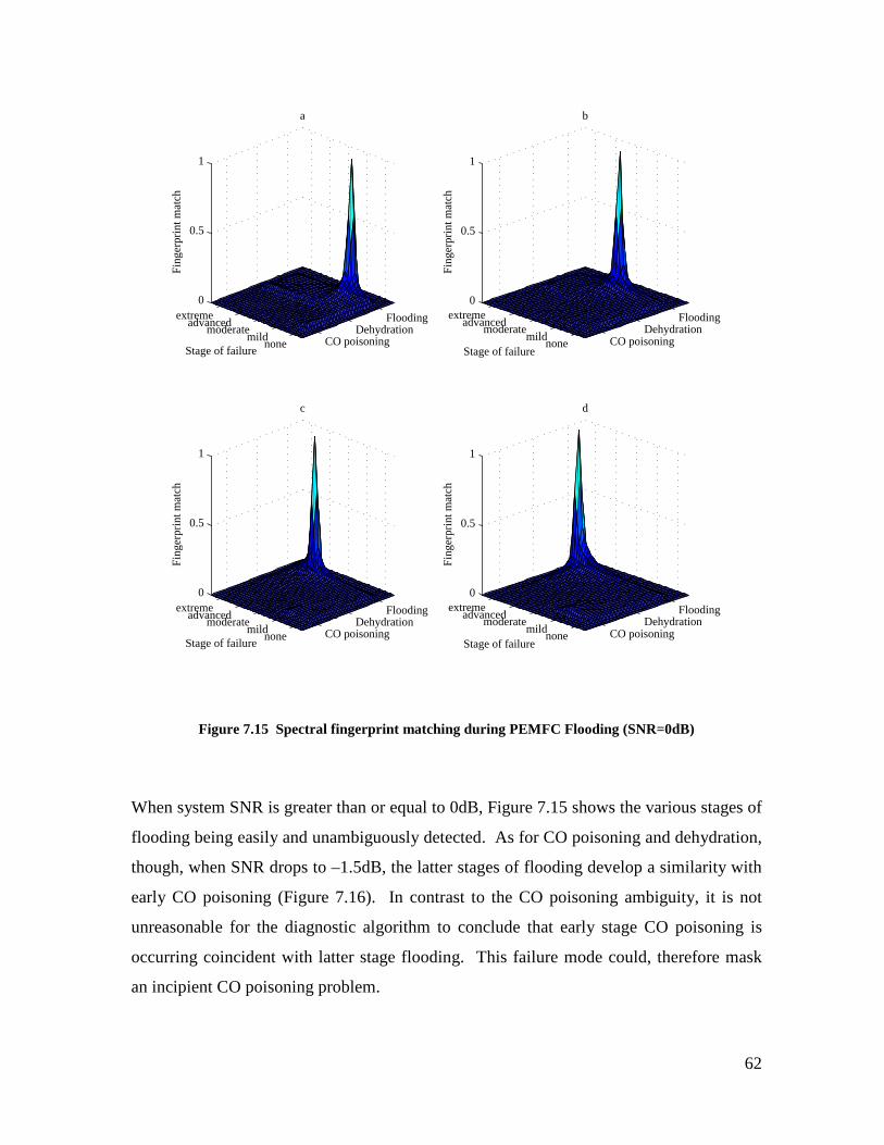
62

CO poisoningDehydration

Flooding

nonemild

moderateadvanced

extreme0

0.5

1

a

Stage of failure

Fin

gerp

rint m

atch

CO poisoningDehydration

Flooding

nonemild

moderateadvanced

extreme0

0.5

1

b

Stage of failure

Fin

gerp

rint m

atch

CO poisoningDehydration

Flooding

nonemild

moderateadvanced

extreme0

0.5

1

c

Stage of failure

Fin

gerp

rint m

atch

CO poisoningDehydration

Flooding

nonemild

moderateadvanced

extreme0

0.5

1

d

Stage of failure

Fin

gerp

rint m

atch

Figure 7.15 Spectral fingerprint matching during PEMFC Flooding (SNR=0dB)

When system SNR is greater than or equal to 0dB, Figure 7.15 shows the various stages of

flooding being easily and unambiguously detected. As for CO poisoning and dehydration,

though, when SNR drops to –1.5dB, the latter stages of flooding develop a similarity with

early CO poisoning (Figure 7.16). In contrast to the CO poisoning ambiguity, it is not

unreasonable for the diagnostic algorithm to conclude that early stage CO poisoning is

occurring coincident with latter stage flooding. This failure mode could, therefore mask

an incipient CO poisoning problem.

63

CO poisoningDehydration

Flooding

nonemild

moderateadvanced

extreme0

0.5

1

a

Stage of failure

Fin

gerp

rint m

atch

CO poisoningDehydration

Flooding

nonemild

moderateadvanced

extreme0

0.5

1

b

Stage of failure

Fin

gerp

rint m

atch

CO poisoningDehydration

Flooding

nonemild

moderateadvanced

extreme0

0.5

1

c

Stage of failure

Fin

gerp

rint m

atch

CO poisoningDehydration

Flooding

nonemild

moderateadvanced

extreme0

0.5

1

d

Stage of failure

Fin

gerp

rint m

atch

Figure 7.16 Spectral fingerprint matching during PEMFC Flooding (SNR=-1.5dB)

Figure 7.10 through Figure 7.16 show data resulting from trials where the experimental

PEMFC state coincides with a fingerprint database entry. This is an optimal situation and

the PEMFC cannot be relied upon to behave as conveniently in practice. However, the

algorithm still produces valid results when the experimental PEMFC state falls between

fingerprint database entries.

64

CO poisoningDehydration

Flooding

nonemild

moderateadvanced

extreme0

0.5

1

a

Stage of failure

Fin

gerp

rint m

atch

CO poisoningDehydration

Flooding

nonemild

moderateadvanced

extreme0

0.5

1

b

Stage of failure

Fin

gerp

rint m

atch

CO poisoningDehydration

Flooding

nonemild

moderateadvanced

extreme0

0.5

1

c

Stage of failure

Fin

gerp

rint m

atch

CO poisoningDehydration

Flooding

nonemild

moderateadvanced

extreme0

0.5

1

d

Stage of failure

Fin

gerp

rint m

atch

Figure 7.17 Spectral fingerprint matching during PEMFC Dehydration (SNR=0dB)

Figure 7.17 shows trials conducted with PEMFC membrane resistance varying between

moderate and advanced dehydration. Panel a represents moderate dehydration, panel b

represents ¼ the evolution between moderate and advanced dehydration, panel c

represents ½ the distance between moderate and advanced dehydration, and panel d

represents ¾ the distance between moderate dehydration and advanced dehydration. In all

cases except ½ the distance between moderate dehydration and advanced dehydration, the

algorithm selects the nearest state. When exactly ½ the distance between moderate

dehydration and advanced dehydration occurs, the algorithm appears to conclude that

moderate and advanced states are equally close. However, this is an artefact of the

imprecise nature of the 3D graph, and the minimum Euclidean distance in this case was

indeed determined to be to moderate dehydration (noise pushed the fingerprint away from

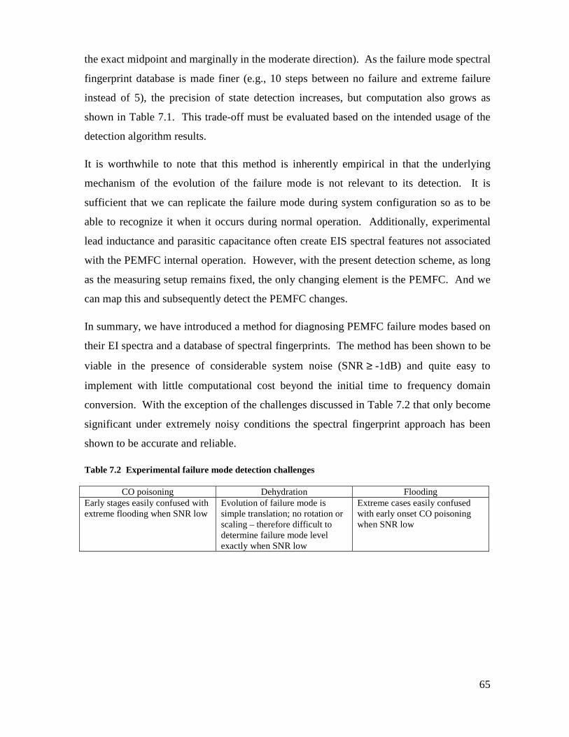
65

the exact midpoint and marginally in the moderate direction). As the failure mode spectral

fingerprint database is made finer (e.g., 10 steps between no failure and extreme failure

instead of 5), the precision of state detection increases, but computation also grows as

shown in Table 7.1. This trade-off must be evaluated based on the intended usage of the

detection algorithm results.

It is worthwhile to note that this method is inherently empirical in that the underlying

mechanism of the evolution of the failure mode is not relevant to its detection. It is

sufficient that we can replicate the failure mode during system configuration so as to be

able to recognize it when it occurs during normal operation. Additionally, experimental

lead inductance and parasitic capacitance often create EIS spectral features not associated

with the PEMFC internal operation. However, with the present detection scheme, as long

as the measuring setup remains fixed, the only changing element is the PEMFC. And we

can map this and subsequently detect the PEMFC changes.

In summary, we have introduced a method for diagnosing PEMFC failure modes based on

their EI spectra and a database of spectral fingerprints. The method has been shown to be

viable in the presence of considerable system noise (SNR ≥ -1dB) and quite easy to

implement with little computational cost beyond the initial time to frequency domain

conversion. With the exception of the challenges discussed in Table 7.2 that only become

significant under extremely noisy conditions the spectral fingerprint approach has been

shown to be accurate and reliable.

Table 7.2 Experimental failure mode detection challenges

CO poisoning Dehydration Flooding Early stages easily confused with extreme flooding when SNR low

Evolution of failure mode is simple translation; no rotation or scaling – therefore difficult to determine failure mode level exactly when SNR low

Extreme cases easily confused with early onset CO poisoning when SNR low

66

8 Conclusions

Three common and important failure modes for PEMFCs, CO poisoning, dehydration, and

flooding, were characterized from the literature and modelled using a two-electrode

Randles approach. This model provided quick and easy access to impedance spectra

allowing simple and expedient experimentation with digital signal processing algorithms

for PEMFC failure mode detection. The model behaviour closely mimics real PEMFC

behaviour reported in the literature.

The PEMFC model was used in a state space simulation to provide time domain EI

spectroscopy experimental data. Frequency domain transformations of the time domain

data provided by the state space approach agreed closely enough with the theoretical

PEMFC frequency response to permit evaluation of a novel pattern recognition-based

failure mode detection algorithm.

Both the PEMFC model and the state space EIS simulation have usefulness beyond this

investigation and can be re-used for other investigations where rapid analysis of PEMFC

behaviour based on published equivalent circuit parameters is required.

The ultimate goal of this work is to develop an EIS-based state of health sensor for

operating fuel cells in which cost, power, and complexity are key design criteria. As a

result, an important objective of this investigation was to minimize the computational

burden so that small, inexpensive, low power consumption digital signal processors can

meet with all of the design constraints while providing effective, real time state of health

detection. The Goertzel algorithm, long employed in DTMF detection for telephony, was

proposed as an alternative to traditional STFT (FFT) approaches and was demonstrated to

offer significant reductions in computation burden, memory size, and computation lag

time with no accuracy penalty.

The Goertzel algorithm is very apt for the multi-frequency EIS approach because it only

calculates the required data without spending computing resources on unnecessary

calculations unlike the STFT approach. Decimation of the time domain signal prior to the

frequency domain transformation was shown to be ill-advised owing to noise constraints.

67

Other multi-frequency EIS improvements such as response sensitive perturbation and

phase optimization were not explored because they have been extensively documented by

other authors (see Chapter 5). However, it is important to note that any on-board PEMFC

state of health sensor, should contemplate these refinements to provide operation across

the greatest possible range of SNR.

The spectral fingerprint concept was introduced and validated for three common and

important PEMFC failure modes, CO poisoning, dehydration, and flooding. The pattern

recognition algorithm employed is computationally very simple and exploits the massive

concentration of EI spectral data into small fingerprints so that it imposes no significant

additional burden on the digital signal processor. It was shown that the spectral

fingerprint approach readily distinguishes between different stages of the described failure

modes when SNR is greater than –1dB. Under circumstances where SNR falls below this

value, the algorithm should not be relied upon as it suffers from failure mode ambiguity

particularly between extreme flooding and mild CO poisoning as well as between all states

of dehydration.

68

9 Suggestions for future work

Failure modes may be easier to detect (more robust to noise) using the present detection

algorithm if a greater number of discrete frequencies are used in the stimulus. It would be

useful to determine the relationship between frequency bins and detection robustness for a

real operating PEMFC by varying the number of frequency bins while monitoring the

fingerprint recognition metric. These experiments must be done with a multi-frequency

approach because of non-stationarity (similar to [20]).

The trade-off to be made is computation burden vs. how critical is the failure mode. For

example, it is imperative that flooding be detected early because once established,

flooding proceeds at an alarmingly fast rate and can damage the cell permanently. While

the same can be said of dehydration with respect to long-term damage, the onset is far

more gradual. It would be worthwhile, then, to spend the extra computing power to obtain

early detection for flooding.

Once the basic technique is proven on operating PEMFCs, the next question becomes,

how many different failure modes can we distinguish. To this end, we need to determine

the relative importance of other contaminants (e.g., SOx, NOx, H2S, NH3, CH4, Fe3+, Ni2+,

Cu2+, Cr3+, Al, Si, K, other sulphur organics, and other hydrocarbons, see [27]) and

characterize them in terms of the Randles cell model used in this paper. With this model

in hand, the same simulation protocol can be used to simulate the failure modes and

determine if sufficient degrees of freedom exist to uniquely identify one failure mode from

another. Following this, the trade-off discussed above must be evaluated for these new

failure modes.

With all the above in hand, and assuming everything works as expected, the next step is to

integrate the EIS fault sensor output into a control algorithm. While a state space or PID

approach is possible, in all likelihood it would present an excessive computational burden

thus squandering the effort made to reduce the computation in the main detection

algorithm. A fuzzy logic approach (see [54]) would probably suffice.

69

References

1. Macdonald, J.R., Impedance spectroscopy: emphasizing solid materials and systems. 1987, New York: John Wiley & Sons.

2. Ivers-Tiffée, E., Weber, A., Schichlein, H., Electrochemical impedance spectroscopy, in Handbook of fuel cells, W. Vielstich, Gasteiger, H. A., Lamm, A., Editor. 2003, John Wiley & Sons.

3. Larminie, J., Dicks, A., Fuel cell systems explained. 2003, Chichester: John Wiley & Sons.

4. Vielstich, W., Gasteiger, H. A., Lamm, A., Handbook of fuel cells, ed. W. Vielstich, Gasteiger, H. A., Lamm, A. Vol. 1. 2003: John Wiley & Sons.

5. Li, X., Principles of fuel cells. 2006, New York: Taylor & Francis. 572. 6. Oldham, K.B. and J.C. Myland, Fundamentals of electrochemical science. 1994,

San Diego, Calif.: Academic Press. xxii, 474. 7. Schulze, M., et al., Combined electrochemical and surface analysis investigation

of degradation processes in polymer electrolyte membrane fuel cells. Electrochimica Acta, 2007. 52(6): p. 2328-2336.

8. Bautista, M., Y. Bultel, and P. Ozil, Polymer electrolyte membrane fuel cell modelling d.c. and a.c. solutions. Chemical Engineering Research & Design, 2004. 82(A7): p. 907-917.

9. Iftikhar, M.U., et al., Dynamic modeling of proton exchange membrane fuel cell using non-integer derivatives. Journal of Power Sources, 2006. 160(2): p. 1170-1182.

10. Ciureanu, M. and R. Roberge, Electrochemical impedance study of PEM fuel cells. Experimental diagnostics and modeling of air cathodes. Journal of Physical Chemistry B, 2001. 105(17): p. 3531-3539.

11. Wang, Y. and C.Y. Wang, Transient analysis of polymer electrolyte fuel cells. Electrochimica Acta, 2005. 50(6): p. 1307-1315.

12. Wagner, N., Characterization of membrane electrode assemblies in polymer electrolyte fuel cells using a.c. impedance spectroscopy. Journal of Applied Electrochemistry, 2002. 32(8): p. 859-863.

13. Andreaus, B., A.J. McEvoy, and G.G. Scherer, Analysis of performance losses in polymer electrolyte fuel cells at high current densities by impedance spectroscopy. Electrochimica Acta, 2002. 47(13-14): p. 2223-2229.

14. Wagner, N. and E. Gulzow, Change of electrochemical impedance spectra (EIS) with time during CO-poisoning of the Pt-anode in a membrane fuel cell. Journal of Power Sources, 2004. 127(1-2): p. 341-347.

15. Merida, W.R., Diagnosis of PEMFC stack failures via electrochemical impedance spectroscopy, in Mechanical Engineering. 2002, University of Victoria: Victoria.

16. Andreaus, B. and G.G. Scherer, Proton-conducting polymer membranes in fuel cells - humidification aspects. Solid State Ionics, 2004. 168(3-4): p. 311-320.

17. Abe, T., et al., Study of PEFCs by AC impedance, current interrupt, and dew point measurements - I. Effect of humidity in oxygen gas. Journal of the Electrochemical Society, 2004. 151(1): p. A101-A105.

18. Knights, S.D., et al., Aging mechanisms and lifetime of PEFC and DMFC. Journal of Power Sources, 2004. 127(1-2): p. 127-134.

70

19. St Pierre, J., et al., Relationships between water management, contamination and lifetime degradation in PEFC. Journal of New Materials for Electrochemical Systems, 2000. 3(2): p. 99-106.

20. Le Canut, J.M., R.M. Abouatallah, and D.A. Harrington, Detection of membrane drying, fuel cell flooding, and anode catalyst poisoning on PEMFC stacks by electrochemical impedance spectroscopy. Journal of the Electrochemical Society, 2006. 153(5): p. A857-A864.

21. Fouquet, N., et al., Model based PEM fuel cell state-of-health monitoring via ac impedance measurements. Journal of Power Sources, 2006. 159(2): p. 905-913.

22. Hakenjos, A., et al., Simultaneous electrochemical impedance spectroscopy of single cells in a PEM fuel cell stack. Journal of Power Sources, 2006. 154(2): p. 360-363.

23. Freire, T.J.P. and E.R. Gonzalez, Effect of membrane characteristics and humidification conditions on the impedance response of polymer electrolyte fuel cells. Journal of Electroanalytical Chemistry, 2001. 503(1-2): p. 57-68.

24. Springer, T.E., et al., Characterization of polymer electrolyte fuel cells using AC impedance spectroscopy. Journal of the Electrochemical Society, 1996. 143(2): p. 587-599.

25. Wei, Z.D., et al., MnO2-Pt/C composite electrodes for preventing voltage reversal effects with polymer electrolyte membrane fuel cells. Journal of Power Sources, 2006. 160(1): p. 246-251.

26. Baschuk, J.J. and X.G. Li, Carbon monoxide poisoning of proton exchange membrane fuel cells. International Journal of Energy Research, 2001. 25(8): p. 695-713.

27. Cheng, X., et al., A review of PEM hydrogen fuel cell contamination: Impacts, mechanisms, and mitigation. Journal of Power Sources, 2007. 165(2): p. 739-756.

28. Hu, J.M., et al., Kinetics investigation of H-2/CO electrooxidation in PEFCs by the combined use of equivalent circuit fitting and mathematical modeling of the faradaic impedance. Electrochimica Acta, 2004. 49(28): p. 5227-5234.

29. Rosa, F., et al., Design of a diesel reformer coupled to a PEMFC. Catalysis Today, 2006. 116(3): p. 324-333.

30. Kawamura, Y., et al., Multi-layered microreactor system with methanol reformer for small PEMFC. Journal of Chemical Engineering of Japan, 2005. 38(10): p. 854-858.

31. Jiang, R.C., H.R. Kunz, and J.M. Fenton, Electrochemical oxidation of H-2 and H-2/CO mixtures in higher temperature (T-cell > 100 degrees C) proton exchange membrane fuel cells: Electrochemical impedance spectroscopy. Journal of the Electrochemical Society, 2005. 152(7): p. A1329-A1340.

32. Ciureanu, M., H. Wang, and Z.G. Qi, Electrochemical impedance study of membrane-electrode assemblies in PEM fuel cells. II. Electrooxidation of H-2 and H-2/Co mixtures on Pt/Ru-based gas-diffusion electrodes. Journal of Physical Chemistry B, 1999. 103(44): p. 9645-9657.

33. Ciureanu, M. and H. Wang, Electrochemical impedance study of anode CO-poisoning in PEM fuel cells. Journal of New Materials for Electrochemical Systems, 2000. 3(2): p. 107-119.

34. Kim, J.D., et al., Effect of CO gas and anode-metal loading on H-2 oxidation in proton exchange membrane fuel cell. Journal of Power Sources, 2001. 103(1): p. 127-133.

71

35. Schiller, C.A., et al., Relaxation impedance as a model for the deactivation mechanism of fuel cells due to carbon monoxide poisoning. Physical Chemistry Chemical Physics, 2001. 3(11): p. 2113-2116.

36. Yang, M.C. and C.H. Hsueh, Impedance analysis of working PEMFCs in the presence of carbon monoxide. Journal of the Electrochemical Society, 2006. 153(6): p. A1043-A1048.

37. Bernardi, D.M. and M.W. Verbrugge, A Mathematical-Model of the Solid-Polymer-Electrolyte Fuel-Cell. Journal of the Electrochemical Society, 1992. 139(9): p. 2477-2491.

38. Bieberle, A. and L.J. Gauckler, State-space modeling of the anodic SOFC system Ni, H-2-H2O vertical bar YSZ. Solid State Ionics, 2002. 146(1-2): p. 23-41.

39. Miller, K.S. and B. Ross, An introduction to the fractional calculus and fractional differential equations. 1993, New York: Wiley. xiii, 366 p.

40. Podlubny, I., Fractional differential equations : an introduction to fractional derivatives, fractional differential equations, to methods of their solution and some of their applications. Mathematics in science and engineering ; v. 198. 1999, San Diego ;Toronto: Academic Press. xxiv, 340.

41. Huet, F., A review of impedance measurements for determination of the state-of-charge or state-of-health of secondary batteries. Journal of Power Sources, 1998. 70(1): p. 59-69.

42. Wiegand, G., K.R. Neumaier, and E. Sackmann, Fast impedance spectroscopy: General aspects and performance study for single ion channel measurements. Review of Scientific Instruments, 2000. 71(6): p. 2309-2320.

43. Gabrielli, C., Identification of electrochemical processes by frequency response analysis. 1998, Solartron.

44. Popkirov, G.S. and R.N. Schindler, A New Impedance Spectrometer for the Investigation of Electrochemical Systems. Review of Scientific Instruments, 1992. 63(11): p. 5366-5372.

45. Blanc, G., et al., Measurement of Electrode Impedance in a Wide Frequency Range Using a Pseudo-Random Noise. Electrochimica Acta, 1975. 20(8): p. 599-601.

46. Blanc, G., et al., Study of Deterministic and Stochastic Behavior of Electrochemical Interface by Means of Numerical Correlation. Journal of Electroanalytical Chemistry, 1975. 62(1): p. 59-94.

47. Gabrielli, C., F. Huet, and M. Keddam, Comparison of Sine Wave and White-Noise Analysis for Electrochemical Impedance Measurements. Journal of Electroanalytical Chemistry, 1992. 335(1-2): p. 33-53.

48. Creason, S.C. and D.E. Smith, Fourier-Transform Faradaic Admittance Measurements .2. Ultra-Rapid, High Precision Acquisition of Frequency-Response Profile. Journal of Electroanalytical Chemistry, 1972. 40(1): p. 1-&.

49. Popkirov, G.S. and R.N. Schindler, Optimization of the Perturbation Signal for Electrochemical Impedance Spectroscopy in the Time-Domain. Review of Scientific Instruments, 1993. 64(11): p. 3111-3115.

50. Darowicki, K. and P. Slepski, Influence of the analyzing window on electrode impedance measurement by the continuous frequency scanning method. Journal of Electroanalytical Chemistry, 2002. 533(1-2): p. 25-31.

72

51. Proakis, J.G. and D.G. Manolakis, Digital signal processing : principles, algorithms, and applications. 2nd ed. 1992, New York, Toronto: Macmillan ;Maxwell Macmillan Canada ; Maxwell Macmillan International. xviii, 969 p.

52. Cooley, J.W. and J.W. Tukey, An Algorithm for Machine Calculation of Complex Fourier Series. Mathematics of Computation, 1965. 19(90): p. 297-301.

53. Schroeder, M.R., Synthesis of Low-Peak-Factor Signals and Binary Sequences with Lol Autocorrelation. Ieee Transactions on Information Theory, 1970. IT16(1): p. 85-+.

54. Schumacher, J.O., et al., Control of miniature proton exchange membrane fuel cells based on fuzzy logic. Journal of Power Sources, 2004. 129(2): p. 143-151.

73

Appendix 1. Simulation of non-integer order transfer function

The electrical behaviour of the PEMFC can be modelled approximately by the equivalent

circuit (Figure 2.4) discussed in Section 2. In this section we explore the time domain

voltage response of the anode or cathode equivalent circuit [9]. The overall cell voltage

response is the sum of the anode, cathode and membrane responses.

( ) ( ) ( ) ( )cell anode membrane cathodev t v t v t v t= + + (A1.1)

R

C

ZW

Figure A1.1 One electrode of PEMFC

Starting with one electrode of the PEMFC, we use the Laplace transform to obtain the

impedance of these circuit elements in terms of the complex variable s.

( ) ( ) ( )( ) ( ) ( ) ( )0

0

1, ,C f

eq f cC f

Z s Z sZ s Z s R Z s

Z s Z s sCs

σ ωω

= = + =+ +

such that

( ) ( )( )( )

1122

1122

0 01 0

0 0 1eq

R sZ s variable s s

sC R s

σω ωω

σω ω

−

−

+ += ∆ = +

+ + +

Now if we make a change of variable 1 0s s ω= +

( )( ) ( )

1 12 2

1 12 2

0 11 0

1 0 0 1 1eq

R sZ s rearrange

s C R s

σωωω σω

−

−

+− =− + +

and rearrange, we obtain

( )1 12 2

12

31 1 12 2 2 2

0 1

1 0 1

1 0 1 0 0 1

1eq

Rs

C CZ s multiply by sRs s R s

C

σ ωω

σω ω σω

−

−

+− =

+ − − +

74

which, when multiplied by 12

1s , results in

( )1 12 2

3 31 12 2 2 2

0 1

1 0

0 0 1 0 1 1

1eq

Rs

C CZ sR s s Rs

C

σ ωω

σω ω σω

+− =

− + − + +

which we then simplify as

( )( )

12

12

312 2

1 32 2

0 11 0

1 0 0 1 1 1 1

A A sV s

I s B B s B s B s

ωω

+−=

− + + +

Now, we cross multiply

( ) ( ) ( ) ( )31 12 2 2

1 3 12 22

1 0 0 1 1 1 1 1 0 0 1V s B B s B s B s I s A A sω ω− + + + = − +

and use the Laplace transform pairs

( ) ( )( ) ( ) ( )

atL e f t F s a

L D f t s F sα α

− = +

=

to obtain

( ) ( ) ( )( ) ( ) ( )( ) ( ) ( )( )( ) ( ) ( )( )

31220 0 0 0

1 32 2

120 0

12

10 1

0

t t t t

t t

B v t e B D v t e B D v t e B D v t e

A i t e A D i t e

ω ω ω ω

ω ω

+ + +

= +

Now if we set

( ) ( ) ( ) ( )0 0t tf t v t e g t i t eω ω= =

we obtain

( ) ( ) ( ) ( ) ( ) ( ) ( ) ( ) ( ) ( )31 122 2

1 3 12 22

10 1 0B f t B D f t B D f t B D f t A g t A D g t+ + + = +

Now we set up the state equations

75

( ) ( )( ) ( ) ( )

( ) ( ) ( ) ( ) ( )( ) ( )( ) ( ) ( ) ( ) ( ) ( )( )( ) ( )

12

1 1 12 2 2

1 1 1 12 2 2 2

1

1 2

2 1 3

3 1 4

f t x t

D x t x t

D x t D D x t x t

D x t D D D x t x t

=

=

= =

= =

giving

( ) ( ) ( ) ( ) ( ) ( ) ( )12

1 3 12 22

0 1 2 1 3 4 0B x t B x t B x t B x t A g t A D g t+ + + = +

So we have

( ) ( ) ( )( ) ( ) ( )( ) ( ) ( )

12

12

12

2 1

3 2

4 3

x t D x t

x t D x t

x t D x t

=

=

=

(A1.2)

and

( ) ( ) ( ) ( ) ( ) ( ) ( )( )12

1 12 2

32

4 0 1 2 1 3 0

1x t B x t B x t B x t A g t A D g t

B= − − − + + (A1.3)

or, in matrix form

( )( )( )

( )( )( )

( ) ( )( )( )

( ) ( ) ( )( )1

2

12

12

12

33 3 3 22 2 2

2 1 1

3 2 2 0

4 3 30 1

0 1 0 0

0 0 1 0

1

x t x t x t

x t x t x t A g t A D g t

x t x t B x tB BBB B B

= = + + − − −

Now, considering the Grünwald – Letnikov fractional derivative

( ) ( )( )

( ) ( )

( )( )

00

0

1lim 1

1

end start

start end

end start

t t

tk

t tt

k

t t

t

kk

D f t y t k tkt

w y t k tt

αα

αα

α−

∆

∆ → =

− ∆

=

= − − ∆ ∆

≈ − ∆∆

∑

∑

(A1.4)

76

where tstart and tend can be considered 0 and t respectively, x is the floor function and

kwα is the product of ( )1k− and the binomial coefficient

( )( ) ( )( )1 2 1

!

n

k k

α α α αα − − − − =

⋯ (A1.5)

( )( )

1

! 1k k k

α αα

Γ + = Γ − +

generalized for real α [39, 40]. Since the factorial and the gamma function both exceed

the machine number limit for approximately k > 170, which reduces the accuracy of our

estimate, we employ a recursive calculation for kwα that is not subject to these limitations

based on expression (A1.5).

0

1

1 0

11 1,2, 1

k

k k

w k

ww w k N

k

α

αα αα

−

= == + = − = −

⋯

(A1.6)

We now assume a small enough ∆t giving

( ) 0

1end start

start end

t t

tend start end start

t t kk

t t t tD y t w y k t

t ttα α

α

− ∆

=

− − ∆ = − ∆ ∆ ∆ ∆ ∑

Substituting end startt tn

t

− = ∆ , separating the first element of the sum, and modifying the

summation limits accordingly, we have

( )( )

( )( ) ( )( )1

10

start end

n

t t kk

D y n t y n t w y n k tt

α αα

=

∆ = − ∆ + − ∆ ∆ ∑

or

( )( )

( ) ( )( )1start endt tD y n t y n t Q n t

tα

α∆ = ∆ + ∆∆

where

77

( ) ( )( )1

n

kk

Q n t w y n k tα

=∆ = − ∆∑

so that finally we have

( )

( )[ ] [ ]( )1

[ ] 0,1,2,3 end startt ty n y n Q n n

tt

αα

− = + = ∆ ∆… (A1.7)

where we now use y[n] and Q[n] as abbreviations for y(n∆t) and Q(n∆t) which are the

discrete time versions of y(t) and Q(t) respectively. Additionally, we introduce the

notation y(α)[n] to represent the discrete non-integer derivative of the function y(t).

Now we can rewrite equations (A1.2) and (A1.3)

( ) [ ] [ ]( ) [ ] [ ]

( ) [ ] [ ] [ ] [ ] [ ] ( ) [ ]

12

12

1 11 12 22 2

3 3 3 3 32 2 2 2 2

1 2

2 3

0 013 1 2 3

0

0

x n x n

x n x n

B AB ABx n x n x n x n g n g n

B B B B B

− =

− =

+ + + = +

and, using result (A1.7), we obtain

( )[ ] [ ]( ) [ ]

( )[ ] [ ]( ) [ ]

12

12

1 1 2

2 2 3

10

10

x n Q n x nt

x n Q n x nt

+ − =∆

+ − =∆

( )[ ] [ ]( ) [ ] [ ] [ ]

[ ]( )

[ ] [ ]( )

12

12

3 3 32 2 2

12

12

3 32 2

0 13 3 1 2 3

0

1

1g

BB Bx n Q n x n x n x n

B B Bt

AAg n g n Q n

B B t

+ + + +∆

= + +∆

or, in matrix form

78

( )

( )

( )

[ ][ ][ ] ( )

[ ][ ]

[ ] ( ) [ ] [ ] [ ]( )

12

1 12 2

12

12

12

3 31 2 22

3 3 32 2 2

1 1

2 2

30

30 1

11 0

1 10 1

1 g

tx n Q n

x n Q nt tx n AA t

Q n g n g n Q nBB B B BB B Bt

− ∆ − − = − ∆ ∆ ∆ − + + + + ∆

Mx = Q

Now we take the inverse of M to solve for -1x = M Q

where

[ ][ ][ ]

( )( )( )

( ) ( )

( )( )

0

1 1

2 2 2

3 3 3

n tx n x n t v n t e

x n x n t x n t

x n x n t x n t

ω ∆ ∆ ∆ = ∆ = ∆ ∆ ∆

x = ,

( )

( )( )

( )( )

( )( ) ( ) ( ) ( ) ( ) ( ) ( )( ) ( )( )

12

12

12

12

11 1 020 02 2

3 32 2

11

21

03

1 1

1

n

kk

n

kk

n nn k tn t n t

k kk k

w x n k t

w x n k tt

AA tw x n k t i n t e i n t e w i n k t e

B Bωω ω

=

=

− ∆∆ ∆

= =

=

− − ∆ − − ∆ ∆ ∆ − − ∆ + ∆ + ∆ + − ∆

∑

∑

∑ ∑

Q

and x(0) = 0.

79

Appendix 2. Equivalent circuit values from the literature

Since the model for the PEMFC that we are employing has not been used in its entirety by

other investigators15, we infer parameters from different studies trying to keep the

experimental conditions and dimensions as similar as possible. For this study, it is the

ability of the algorithms discussed herein to detect and identify changes occurring within

the model via EIS that is of significance rather than the fidelity of this model to any

particular fuel cell.

EIS data is available for experiments carried out on a PEMFC at 80°C with a Nafion 117

membrane, symmetric E-TEK electrodes (20% Pt/C, 0.4mg·cm-2, 200µm thickness, 23

cm2 geometric surface area) impregnated with 1mg·cm-2 Nafion suspension, humidified

anode H2 and dry cathode O2 gas feed at 2 bar absolute, dead end H2 flow and O2

stoichiometry of λ=8 [12]. The EIS data can be fit to the equivalent circuit of Figure 2.4

using the following approach:

1. Rs can be easily inferred from the high frequency end of the magnitude Bode plot.

At high frequency, the double layer capacitors behave as short circuits leaving Rs

as the sole real impedance in the equivalent circuit.

2. Rct,a and Rct,c. These values can be inferred from the two extremes of the

magnitude Bode plot.

, ,ct total left right ct total sZ Z Z R R= − = − (A2.1)

In the same study, io,anode and io,cathode were obtained for H2:H2 and O2:O2 operation.

Using these io values together with the , , , ,ct total ct total ct anode ct cathodeR Z R R= = + values

and relationship (2.6), we can obtain an approximate value for Rct,a and Rct,c over

the range of experimental current densities. Note that this approach fails at high

15 Instead they have used subsets of this circuit depending on which element represented the behaviour under investigation. For example, catalysis studies tend to ignore the Warburg impedance focusing instead on the Rct-Cdl elements. Other studies concerning O2 diffusion include the Warburg impedance but ignore the anode contribution.

80

current densities because the diffusion limitation begins to appear. In such cases,

we extrapolate the horizontal section of the magnitude bode plot to find ,ct totalZ .

3. Now we turn to the double layer capacitances, Cdl,a and Cdl,c. We can calculate

Cdl,total from the pole frequency in the magnitude Bode plot together with Rct,total.

Now, in order to discover the respective anode and cathode contribution we note

, ,

, ,

, ,,

,

o r anode eff anode

dl anode H anode

o r cathode eff cathodedl cathode

H cathode

A

C dAC

d

ε ε

ε ε= (A2.2)

and

( )

1 1 1

3 22 2

2 3

3 21

1311 1

44

3 2 2

44

3 2 2

part

part

eff geom molar surf

molar grav surf

eff geom grav

A A L M V D A U

mg mol particle cm cmcm cm

cm mg cm mol particle

d dV D D M A

d dA A L M D M

π π

π π

− − −

−

−−− −

= ⋅ ⋅ ⋅ ⋅ ⋅ ⋅

= ⋅ ⋅ ⋅ ⋅ ⋅

= = =

= ⋅ ⋅ ⋅ ⋅ ⋅

( )

2

16eff geom grav

U

A A L D Ud

−

⋅

= ⋅ ⋅ ⋅ ⋅

(A2.3)

where A, L, M, V, D, and U represent area, loading, molar mass, volume, density,

and utilization, respectively. Since the anode and cathode electrodes are

symmetric, Ageom, L, d, Dgrav, and U are the same and therefore Aeff,anode = Aeff,cathode.

, , ,

, , ,

dl anode r anode H cathode

dl cathode r cathode H anode

C d

C d

εε

= (A2.4)

The anode and cathode double layer compositions, however, are quite different and

εr,anode ≠ εr,cathode and dH,anode ≠ dH,cathode. The ionic species at the anode are

hydrated protons forming a layer of aligned water molecules for which the

dielectric constant is 6 rather than the unaligned water dielectric constant of 80

(ref: Modern electrochemistry). At the cathode surface, the precise ionic

81

composition is unknown, but the tight monolayer of aligned water molecules is

unlikely. Further, any anions lining the cathode surface will be large compared to

the proton such that this double layer is likely to be several times thicker and more

diffuse than that of the anode. The effects of thickness and dielectric constant are

opposite in (A2.4) so for simplicity, we set Cdl,anode = Cdl,cathode resulting in

, , ,2dl anode dl cathode dl totalC C C= = .

4. The dominant diffusion processes at each electrode influencing the Warburg

impedances involve water transport on the anode side and oxygen gas transport on

the cathode side [13]. The time constants for these processes have been shown to

be on the order of 10 seconds for the anode and 0.01 to 0.1 seconds for the cathode

[11]. We are then left with determining the current density dependent A(j)

parameter from (2.10). We fit this last parameters by trial and error with the

constraint that Aa(j) has been reported as 3 orders of magnitude smaller than Ac(j)

in a symmetrical fuel cell [9].

Table A2.1 Equivalent circuit parameters derived from the literature

Cell voltage (V) 0.984 0.900 0.797 0.697 0.597 0.497 0.397 Current density (mA·cm-2) 0.004 5.814 93.00 254.4 405.0 516.8 622.1 Power density (mW·cm-2) 0.004 5.233 74.12 177.3 241.8 256.8 246.9

Rct,a (µ Ω) 342.2 15.20 1.600 1.100 1.000 1.200 1.400 Rct,c (Ω) 5.704 0.253 0.026 0.018 0.017 0.020 0.023 Rs (mΩ) 10.00 10.00 10.00 10.00 10.00 10.00 10.00 Cdl,a (F) 0.100 0.100 0.100 0.100 0.100 0.100 0.100 Cdl,c (F) 0.100 0.100 0.100 0.100 0.100 0.100 0.100 Aa (µΩ) 0.000 0.000 0.000 0.000 5.000 10.00 15.00 Ac (mΩ) 0.000 0.000 0.000 0.000 5.000 10.00 15.00 τa (sec) 0.100 0.100 0.100 0.100 0.100 0.100 0.100 τc (sec) 10.00 10.00 10.00 10.00 10.00 10.00 10.00

The resulting equivalent circuit parameters are collected in Table A2.1 and the

corresponding impedance plots are shown in Figure 2.7 and Figure 2.8.

82

Appendix 3. Matlab program listings

These are rather extensive to list and are available from the author in electronic form

(ivsm at telus dot net).